Making Data Structures Confluently Persistent

Making Data Structures Confluently Persistent∗

Amos Fiat† Haim Kaplan‡

Reality is merely an illusion, albeit a very persistent one.

— Albert Einstein (1875-1955)

Abstract

We address a longstanding open problem of [11, 10], and present a general transformation that

transforms any pointer based data structure to be confluently persistent. Such transformations for fully

persistent data structures are given in [11] , greatly improving the performance compared to the naive

scheme of simply copying the inputs. Unlike fully persistent data structures, where both the naive scheme

and the fully persistent scheme of [11] are feasible, we show that the naive scheme for confluently persistent

data structures is itself infeasible (requires exponential space and time). Thus, prior to this paper there

was no feasible method for making any data structure confluently persistent at all. Our methods give an

exponential reduction in space and time compared to the naive method, placing confluently persistent

data structures in the realm of possibility.

1 Introduction

We call the initial configuration of a data structure version zero. Every subsequent update operation creates

a new version of the data structure. A data structure is called persistent if it supports access to multiple

versions and it is called ephemeral otherwise. The data structure is partially persistent if all versions can be

accessed but only the newest version can be modified. The structure is fully persistent if every version can

be both accessed and modified. Since the seminal paper of Driscoll, Sarnak, Sleator, and Tarjan (DSST)

[11], and over the part fifteen years, there has been considerable development of persistent data structures.

Persistent data structures have important applications in various areas such as functional programming;

text, program, and file editing and maintenance; computational geometry; and other algorithmic application

areas. (See [4, 5, 6, 9, 10, 11, 19, 20, 21] and references therein)

DSST developed efficient general methods to make pointer-based data structures partially or fully per-

sistent. These methods support updates that apply to a single version of a structure at a time, but they

do not accommodate operations that combine two different versions of a structure, such as set union or

list catenation. We call an update operation that applies to more than a single version a meld operation1.

DSST posed as an open question whether there is a way to generalize their result to allow meld operations.

∗A Preliminary Version of this paper has appeared in the Proceedings of the 12th Annual Symposium on Discrete Algorithms,

2001.†School of computer science, Tel Aviv University, Tel Aviv 69978, [email protected]‡School of computer science, Tel Aviv University, Tel Aviv 69978, [email protected]. Research supported in part by

the Israel Science Foundation (grant no. 548).1We remark that some specific data structures have a meld operation associated with them that operates on a single version.

In this paper we use meld as a generic name for operations that operate on multiple versions.

1

x=1, y=2

x=6 x=3

x=6

y=2

y=12

y=17

y=5

y=2

y=2

x=6

x=3

x=3

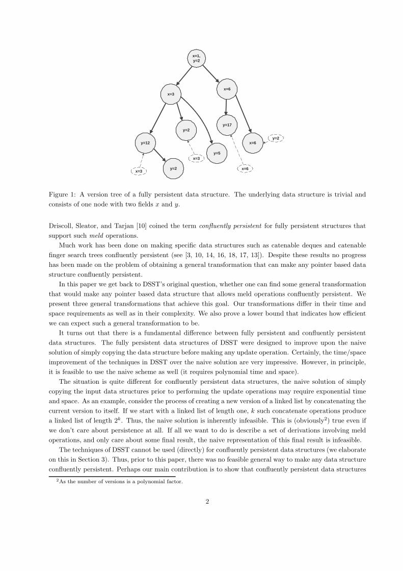
Figure 1: A version tree of a fully persistent data structure. The underlying data structure is trivial and

consists of one node with two fields x and y.

Driscoll, Sleator, and Tarjan [10] coined the term confluently persistent for fully persistent structures that

support such meld operations.

Much work has been done on making specific data structures such as catenable deques and catenable

finger search trees confluently persistent (see [3, 10, 14, 16, 18, 17, 13]). Despite these results no progress

has been made on the problem of obtaining a general transformation that can make any pointer based data

structure confluently persistent.

In this paper we get back to DSST’s original question, whether one can find some general transformation

that would make any pointer based data structure that allows meld operations confluently persistent. We

present three general transformations that achieve this goal. Our transformations differ in their time and

space requirements as well as in their complexity. We also prove a lower bound that indicates how efficient

we can expect such a general transformation to be.

It turns out that there is a fundamental difference between fully persistent and confluently persistent

data structures. The fully persistent data structures of DSST were designed to improve upon the naive

solution of simply copying the data structure before making any update operation. Certainly, the time/space

improvement of the techniques in DSST over the naive solution are very impressive. However, in principle,

it is feasible to use the naive scheme as well (it requires polynomial time and space).

The situation is quite different for confluently persistent data structures, the naive solution of simply

copying the input data structures prior to performing the update operations may require exponential time

and space. As an example, consider the process of creating a new version of a linked list by concatenating the

current version to itself. If we start with a linked list of length one, k such concatenate operations produce

a linked list of length 2k. Thus, the naive solution is inherently infeasible. This is (obviously2) true even if

we don’t care about persistence at all. If all we want to do is describe a set of derivations involving meld

operations, and only care about some final result, the naive representation of this final result is infeasible.

The techniques of DSST cannot be used (directly) for confluently persistent data structures (we elaborate

on this in Section 3). Thus, prior to this paper, there was no feasible general way to make any data structure

confluently persistent. Perhaps our main contribution is to show that confluently persistent data structures

2As the number of versions is a polynomial factor.

2

Ver #1

#4 #2

#5

#3

#7

#6

#9

#8

#10 #12 #11

Merge Red/Black Trees

Increment all keys by 2

Merge three R/B trees, remove bottom 1/2 of

keys

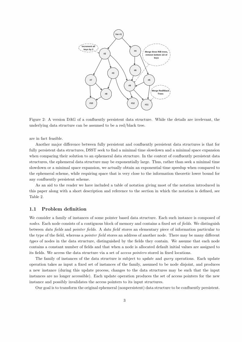
Figure 2: A version DAG of a confluently persistent data structure. While the details are irrelevant, the

underlying data structure can be assumed to be a red/black tree.

are in fact feasible.

Another major difference between fully persistent and confluently persistent data structures is that for

fully persistent data structures, DSST seek to find a minimal time slowdown and a minimal space expansion

when comparing their solution to an ephemeral data structure. In the context of confluently persistent data

structures, the ephemeral data structure may be exponentially large. Thus, rather than seek a minimal time

slowdown or a minimal space expansion, we actually obtain an exponential time speedup when compared to

the ephemeral scheme, while requiring space that is very close to the information theoretic lower bound for

any confluently persistent scheme.

As an aid to the reader we have included a table of notation giving most of the notation introduced in

this paper along with a short description and reference to the section in which the notation is defined, see

Table 2.

1.1 Problem definition

We consider a family of instances of some pointer based data structure. Each such instance is composed of

nodes. Each node consists of a contiguous block of memory and contains a fixed set of fields. We distinguish

between data fields and pointer fields. A data field stores an elementary piece of information particular to

the type of the field, whereas a pointer field stores an address of another node. There may be many different

types of nodes in the data structure, distinguished by the fields they contain. We assume that each node

contains a constant number of fields and that when a node is allocated default initial values are assigned to

its fields. We access the data structure via a set of access pointers stored in fixed locations.

The family of instances of the data structure is subject to update and query operations. Each update

operation takes as input a fixed set of instances of the family, assumed to be node disjoint, and produces

a new instance (during this update process, changes to the data structures may be such that the input

instances are no longer accessible). Each update operation produces the set of access pointers for the new

instance and possibly invalidates the access pointers to its input structures.

Our goal is to transform the original ephemeral (nonpersistent) data structure to be confluently persistent.

3

To that end we provide a representation for the family of the instances that allows us to simulate an update

operation such that it does not damage the structures that it takes as input. This way each update operation

creates a new version of the data structure, that coexists with all previous versions.

We describe all versions of a confluently persistent data structure by a version DAG. A version DAG is

an acyclic directed graph D = (V, E). We assume that the version DAG has a single source vertex rt such

that all v ∈ V are reachable from rt. We also assume that D has no parallel edges.3 Every vertex v ∈ V is

associated with a version of the data structure, an edge (u, v) implies that the version associated with v was

produced by taking as an input the version associated with u. Since a new version depends only on versions

already in existence the graph must be acyclic. We refer to version u, u ∈ V , rather than use the more

cumbersome “the version associated with vertex u”. We also use the notation Du to refer to version u of the

data structure. In case the data structure does not support a meld operation the version DAG is a tree and

we degenerate to the fully persistent setting studied by DSST. See Figure 1 for an example of a version tree

of a fully persistent data structure and Figure 2 for an example of a version DAG of a confluently persistent

data structure.

1.2 Model of computation, performance measures, and some terminology

Following the footsteps of DSST we break each update or access operation into its elementary components.

We distinguish three such components.

1. A retrieval of a field value. We shall often distinguish between a retrieval of the value in a data field

and a retrieval of the value in a pointer field.

2. An assignment of a value to a field.

3. An allocation of a new node.

We shall denote by U the total number of assignment operations4 (steps of type (2)) and by T the total

number of field retrievals (steps of type (1)). Note that:

1. The total number of nodes we allocate (steps of type (3)) is smaller than U , as each allocation is

followed by assigning default values to the fields of the new node, and assigning the address of the new

node into some other field.

2. When a new version is created, we perform at least one assignment. Thus, the number of versions is

at most U .

3. The number of assignments U is O(T ). This holds since in order to do an assignment we first have to

retrieve the address of the node containing the field to which we want to assign. (Recall that there are

only constant number of fields in each node.)

We will compare our persistent data structures by measuring the time and space they require for each

field retrieval and for each assignment. Note that the time for allocating nodes will always be dominated by

the time for assignments. To traverse an arbitrary pointer based data structure constructed by performing U

assignment, one must “remember” all U assignments. Thus, the memory space of any machine implementing

3These assumptions are to simplify the presentation only and can be eliminated easily. For example, to simulate a meld

operation that takes two copies of the same version we first duplicate this version by an explicit update operation.4In case an update operation performs multiple assignments to the same field of the same node we count only the last such

assignment.

4

such a data structure must be Ω(U), and an address consists of Ω(logU) bits (all logs are base 2 in this

paper). We therefore assume throughout this paper that the actual implementation is on a Random Access

Machine (RAM), with word length Θ(logU).

As a main tool in our exposition we use the following very simple transformation that makes any pointer

based data structure confluently persistent. We call it the naive scheme. In this scheme before updating

a version or several versions to create a new version we first copy the input version/versions and make the

changes on the new copies.

1.2.1 High Level Goals.

The naive scheme maintains the versions completely node disjoint and thereby require a large amount of

memory, and a large amount of time for node copying. However, if we do not count node copying but only

look at the time and space requirements for an individual retrieval or assignment then the naive scheme is

as efficient as doing the operations on independent ephemeral data structures. It thus seems that the main

goal in designing efficient persistent data structures is to attempt to avoid the time/space costs of copying

the input, at the possibly added expense of increasing the time/space per retrieval and/or assignment.

This goal indeed captures the work of DSST for fully persistent data structures. In the context of

confluently persistent data structures one can aim for (and achieve) much more. In the confluently persistent

setting the ephemeral costs are much larger than in the fully persistent settings. Therefore it is possible to

avoid node copying while at the same time simulating field retrievals and assignments much faster than the

naive scheme.

1.2.2 Fully Persistent versus Confluently Persistent Data Structures.

We now seek to explain the inherent difference between confluently persistent and fully persistent data

structures. Note that if we apply the naive scheme to obtain a fully persistent structure (i.e. we never

perform a meld operation) then the total number of nodes in all versions is O(U2). This follows for the fully

persistent setting as the number of nodes in any particular version is at most U . Each node of a particular

version can be associated with a specific allocation (maybe in another version) such that no two nodes in

the same version are associated with the same allocation. Therefore in the fully persistent setting we can

implement the naive scheme using O(U2) words each consisting of O(logU) bits5. The situation in the

confluently persistent setting is fundamentally different.

In the confluently persistent setting the number of nodes in a single version can be as high as 2Ω(U).

As an example recall the linked list mentioned earlier, initially consisting of a single node, that is being

concatenated with itself Θ(U) times. The final list contains 2Θ(U) nodes. Therefore in the confluently

persistent setup we may not be able to implement the naive scheme with memory polynomial in U .

To quantify the memory requirements of the naive scheme more precisely we need the following definitions.

Let D be a version DAG, let v be a node in the DAG, and let R(v) be the set of all different paths from

the root, rt, to v in D. We define the depth of v, denote by d(v), as the length of the longest path in R(v).

We define the effective depth of v, and denote it by e(v), as the logarithm of the number of different paths

from rt to v in D plus 1, i.e. e(v) = log(|R(v)|) + 1. Note that the effective depth of v may be smaller than

the depth of v, as is the case when the DAG is a tree. For a tree the effective depth of every node is one,

whereas the depth of a node v is the length of the path from rt to v. It is also easy to construct examples

where the effective depth of a node is larger than its depth. We define the depth of the DAG D, denoted by

5This is the memory required for pointers to the different assignment values, in addition to this we need to store the actual

assignment values themselves.

5

d(D), as the largest depth of a node in D. Similarly we define the effective depth of D, denoted by e(D),

as the largest effective depth of a node in the DAG. One can view e(D) as a measure of the deviation of D

from being a tree.

Consider a version v of a confluently persistent data structure implemented by the naive scheme. We

associate each node w in Dv with a specific allocation of a node s(w) in v or in a version u that is an ancestor

of v in the DAG. Formally we define node s(w) to be either w itself if w was allocated in v, otherwise, w is a

copy (after, possibly, some assignments) of w′ from some predecessor version of v in the DAG.We recursively

define s(w) = s(w′). We call s(w) the seminal node of w.

In the confluently persistent setup many nodes in version v can be associated with the same seminal

node. However it is easy to see that the total number of nodes in version v associated with the same seminal

node is no larger than the number of paths from rt to v and therefore not larger than 2e(v). It follows that

the total number of nodes in a single version of a confluently persistent data structure may be as high as

Θ(U · 2e(D)), and the total number of nodes in all versions may be as high as Θ(U2 · 2e(D)).

To give unique names to these nodes we need (in total) Θ(U2 · 2e(D)(e(D)+ logU)) bits. Note that when

D is a tree then e(D) = 1 and this expression reduces to the Θ(U2 logU) bits required by the naive scheme

in the fully persistent setting. Since each address of the naive scheme consists of O(1+ e(D)log U ) words it follows

that the time it takes for the naive scheme to simulate an assignment or a retrieval is Ω(1+ e(D)logU ). See Table

1 for a summary of the resources required by the naive scheme in the fully persistent and the confluently

persistent settings.

1.2.3 A Paradox and its Intuitive Resolution.

In contrast to the fully persistent setting our best confluently persistent schemes require only memory

polynomial in U while at the same time improving exponentially the ephemeral time costs. This may seem

to be paradoxical at a first glance.

We now give a high level intuitive explanation as to how this paradox is resolved. The high ephemeral

time costs are due to extensive use of memory that makes the addresses become very long. Many of these

exponentially many nodes that the naive scheme allocates share the same values in all their data fields6. Our

schemes refrain from representing all these identical nodes explicitly, and use a compressed representation

for pointer fields. We do this while keeping the ability to simulate field retrievals and assignments efficiently.

1.3 Some Fundamental Technical Elements from DSST

DSST first considered the fat node method . The fat node method works by allowing a field in a node of the

data structure to contain a list of values arranged in a binary search tree. This list is sorted according to a

linear order of the versions that is consistent with some preorder traversal of the version tree. This linear

order is maintained using an external structure developed by Dietz and Sleator [7]. To get the value of a

field in some particular version one has to perform a binary search on the sorted list of field values.

The fat node method requires only a constant number of words per assignment. Therefore its total space

requirement is only O(U logU) bits compared to O(U2 logU) bits of the naive scheme. This space efficiency

comes at a cost of increasing the time requires for field retrieval and assignment. Rather than O(1) time in

the naive scheme we now may need O(logU) time to perform a binary search.

DSST managed to improve the fat node method and reduce this penalty in time. Using a technique

they called node splitting they obtain a fully persistent data structure that requires only O(1) time per field

6Although their pointer fields will in general be different.

6

retrieval or assignment. See Table 1 for a summary of the time and space requirements of the fat node and

node splitting methods.

The navigation mechanism used by the transformations of DSST does not generalize to the case where

the version graph is a DAG rather than a tree. It is inherently incapable of handling nodes originating from

the same seminal node in a single version. Since both the fat node method and the node splitting method

rely on it, neither of these methods works in the confluently persistent setting. It follows that the only

working solution that we have is the naive scheme. But the naive scheme may also be infeasible as it requires

memory which is exponential in the number of updates. Therefore, prior to this work, there was no obvious

solution whose memory requirements are bounded by a polynomial in U even if we are willing to sacrifice

the time bounds for field retrieval and assignment.

1.4 Overview of Our Results.

Our first result, presented in Section 2 is a lower bound on the space requirement of any general scheme

to make a data structure confluently persistent. We show that for any such scheme, and a DAG D, we

can associate operations with the vertices of D such that some assignments would require Ω(e(D)) bits.

Thus, the space that the naive scheme uses per assignment is essentially the best we can hope for without

compromising the generality of our approach.

The rest of the paper presents several methods to make data structures confluently persistent, while

avoiding the exponential costs of node copying. Several basic ideas are shared by our methods, and they

differ in the time/space tradeoffs they generate. The truly fast schemes are randomized. The different

time/space costs for the various schemes are presented in Table 1.

In the first row of Table 1 we give the requirements of the naive scheme. To actually implement the naive

scheme would require that we copy an exponential number of nodes with an associated exponential time

requirement. Following DSST we compare the performance of our various schemes to the performance of

the naive scheme where node copying (and it’s associated memory) is for free. We refer to these time/space

costs as the ephemeral costs, as they reflect the time/space requirements of performing the appropriate

operations on a non-persistent version of the data structure. As noted previously for confluently persistent

data structures the naive scheme may require exponential computation and is referenced here mainly for

purposes of comparison.

The ratio between the space requirement per assignment for a given confluently persistent scheme and

the ephemeral cost in space per assignment (or equivalently, the lower bound on space per assignment) is

called the space expansion of the scheme.

Let r1 be the ratio between the time required for assignment by a confluently persistent scheme and the

ephemeral cost in time for assignment, let r2 be the ratio between the time required for retrieval by the

scheme and the ephemeral cost in time for retrieval. Let r = maxr1, r2, we define the time slowdown of

the scheme to be r if r ≥ 1, we define the time speedup of the scheme to be 1/r if r < 1.

Note that the measures of space expansion, time slowdown, and time speedup, are all based on the

ephemeral costs. Thus, in a comparison with the naive scheme, these measures all discriminate in favor of

the naive scheme in the sense that they ignore the costs associated with node copying for the naive scheme

whereas the confluently persistent scheme is charged for everything.

All our algorithms use fat nodes in a way similar to the fat node method of DSST. Each fat node f

corresponds to a specific allocation of a node s by some update operation. Fat node f represents all nodes w

of the naive scheme that are derived from s by node copying, i.e. all nodes w such that s(w) = s. For a fat

node f , we denote by N(f) the set of nodes of the naive scheme that it represents. To identify a particular

7

Schemes Total # of bits Space (# words) Time per Time per

(for all versions) per Assignment Assignment Retrieval

Confluently Persistent

“Ephemeral costs”

naive scheme O

(U2 · 2e(D)

× (e(D) + logU)

)O(1 +

e(D)log U

)O(1 +

e(D)log U

)O(1 +

e(D)log U

)

Any Scheme

(Info. Theory

Lower Bound)

Ω (U · e(D)) Ω(1 +

e(D)log U

)

Full Path O(U · d(D) logU) O(d(D)) O(d(D) + logU) O(d(D) + logU)

Comp. Path O(U · e(D) logU) O(e(D)) O(e(D) + logU) O(e(D) + logU)

Rand.

Full PathO(U · d(D) log T ) O

(d(D) log T

log U

)O(log3(d(D)) log T

logU

)O(log2(d(D)) log T

log U

)

Rand.

Comp. PathO(U · e(D) log T ) O

(e(D) log T

logU

)O

(logU

+ log3(e(D)) log TlogU

)O

(logU

+log2(e(D)) log Tlog U

)

Fully Persistent (For Comparison, from DSST)

“Ephemeral costs”

naive scheme O(U2 log U) O(1) O(1) O(1)

Fat nodes O(U log U) O(logU) O(logU) O(logU)

Node splitting O(U log U) O(1) O(1) O(1)

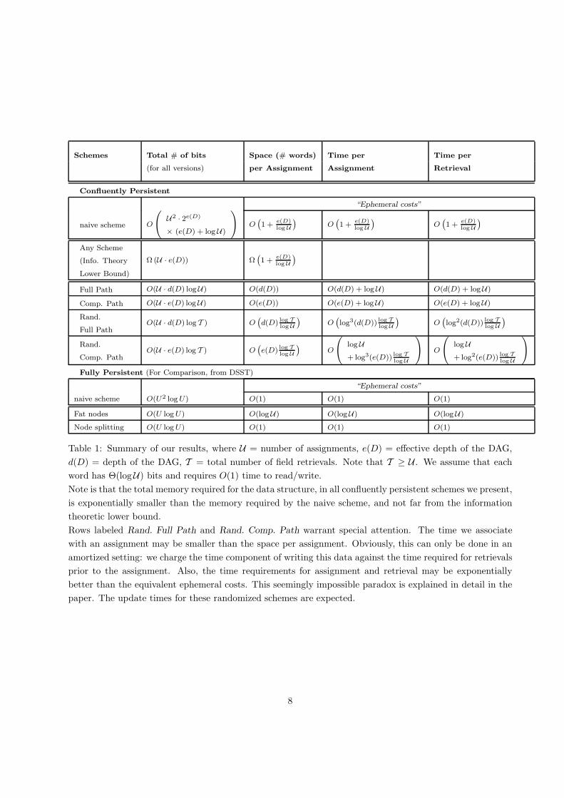
Table 1: Summary of our results, where U = number of assignments, e(D) = effective depth of the DAG,

d(D) = depth of the DAG, T = total number of field retrievals. Note that T ≥ U . We assume that each

word has Θ(logU) bits and requires O(1) time to read/write.

Note is that the total memory required for the data structure, in all confluently persistent schemes we present,

is exponentially smaller than the memory required by the naive scheme, and not far from the information

theoretic lower bound.

Rows labeled Rand. Full Path and Rand. Comp. Path warrant special attention. The time we associate

with an assignment may be smaller than the space per assignment. Obviously, this can only be done in an

amortized setting: we charge the time component of writing this data against the time required for retrievals

prior to the assignment. Also, the time requirements for assignment and retrieval may be exponentially

better than the equivalent ephemeral costs. This seemingly impossible paradox is explained in detail in the

paper. The update times for these randomized schemes are expected.

8

node w of the naive scheme in our simulation we use a path in the DAG. This is the path from s(w) to w

that goes through every version v which contains a node w′ from which w is derived by a series of node copy

operations. Every fat node stores all values assigned to its fields in all the nodes that it represents. Our

different algorithms differ in how they represent the fat nodes and in how they represent paths in the DAG.

1.4.1 The Full Path Method.

Our first and the simplest method to make a data structure confluently persistent is the full path method.

This method represents a path in the DAG by the list of versions it contains. It represents the values of each

field in a fat node in a trie. Each value is identified by the path that corresponds to the node in which this

value was assigned. The full path method gives a deterministic confluently persistent data structure such

that the space cost of an assignment is at most O(d(D)) words.

Since d(D) may be much larger than O(e(D)) the space expansion of the full path method may be large.

In particular if D is a tree, (I.e., we are not really dealing with a confluently persistent data structure since

no melds take place), then the performance of the full path method would be much worse than that of the fat

node method of DSST. The time per field retrieval and an assignment of this method is O(d(D) + logF) =

O(d(D) + logU) where F is the maximum number of assignments that we do to a particular field in the

family N(f) of all nodes associated with a fat node f . The full path method is described in Section 4.

1.4.2 The Compressed Path Method.

Our second method is the compressed path method. Our motivation in designing this method was to enhance

the full path method so it reduces to the fat node method of DSST in case the DAG is a tree. In general, the

performance of the compressed path method is a function of the effective depth of the DAG, e(D), which is a

measure of the deviation of the DAG from being a tree. When e(D) = 1 (the DAG is a tree) the compressed

path method reduces to the fat node method of DSST.

The essence of the compressed path method is a particular partition of our DAG into disjoint trees. This

partition is defined such that every path enters and leaves any specific tree at most once. The compressed

path method encodes paths in the DAG as a sequence of pairs of versions. Each such pair contains a version

where the path enters a tree T and the version where the path leaves the tree T . We show that the length

of each such representation is O(e(D)). Each value of a field in a fat node is now associated with the

compressed representation of the path of the node in N(f) in which the corresponding assignment occurred.

A key property of these compressed path representations is that they allow easy implementations of certain

operations on paths.

The space expansion of the compressed path method is O(logU): As assignment requires up to O(e(D))

words each of O(logU) bits. The time slowdown of the compressed path method is also O(logU): Searching

or updating the trie representing all values of a field in a fat node requires O(e(D) + logU) time. The

compressed path method is described in Section 5.

1.4.3 Randomized Methods.

Our last two methods the randomized full path method and the randomized compressed path method are

variations of the full path method and the compressed path method, respectively. Surprising, they actually

attain significant time speedup over the naive scheme at the expense of a (slightly) larger space expansion

than that of the non-randomized algorithms. These methods make use of randomization and have some

polynomially small probability of inaccurately representing our collection of versions.

9

Our randomized methods encode each path (or compressed path) in the DAG by an integer. We assign to

each version a random integer, and the encoding of a path p is simply the sum of the integers that correspond

to the versions on p. Each value of a field in a fat node is now associated with the integer encoding the path

of the node in N(f) in which the corresponding assignment occurred. To index the values of each field we

use a hash table storing all the integers corresponding to these values.

To deal with values of pointer fields we have to combine this encoding with a representation of paths in

the DAG (or compressed paths) as balanced search trees, whose leaves (in left to right order) contain the

random integers associated with the vertices along the path (or compressed path)7.

This representation allows us to perform certain operations on these paths in logarithmic (or poly-

logarithmic) time whereas the same operations required linear time using the simpler representation of paths

in our non-randomized methods. In particular, we can compute the integer associated with of a prefix of a

path by splitting the corresponding balanced binary tree in logarithmic time.

To put everything together we need these binary search trees to be confluently persistent themselves. We

achieve that by the path copying method of DSST. According to this method we duplicate every node which

changes while updating the tree. Since only logarithmically many nodes change with split or concatenate

operations, every field retrieval or assignment (on the larger confluently persistent data structure) requires

no more than logarithmic time and space.

The size of each random integer which we assign to a version depends on the total number of steps

the simulation performs. I.e., it depends both on the number of field retrievals and on the number of

assignments. Specifically the space required per assignment grows by a factor of log T / logU . The time

bounds however, are now polylogarithmic in d(D) and e(D) in the randomized full path method and in the

randomized compressed path method, respectively. Thus if T is polynomial in U the randomized compressed

path method has a time speedup of Ω(e(D)/polylog(e(D))).

2 A Simple Lower Bound

We first recall the following definition from Section 1.2.2. Let R(u) be the set of paths in the version

DAG between the root and the vertex u. The effective depth of the version associated with a vertex u is

e(u) = log |R(u)| + 1.

We also define an instantiation of a version DAG, D = (V, E), denoted ID, is the assignment of an

update operation, ID(u), to every vertex u ∈ V . The update operation ID(u) takes as input access pointers

to the data structures Dv|(v, u) ∈ E, The output of ID(u) is a set of access pointers to the data structure

Du resulting from the operation of ID(u) on the set of data structures Dv|v ∈ P (u). With this terminology

we can state our lower bound as follows.

Theorem 2.1 Let D = (V, E) be a version DAG and let k = Ω(|E|2). For any vertex u ∈ V such that

e(u) > 2 log k, there exists an instantiation ID with k assignments at node u such that any representation of

Du requires Ω(e(u))) bits on average for each of these k assignments.

Proof: The data structure we use to define the instantiation is a red/black binary tree. We don’t use the

search properties of the red/black tree, but only make use of the color bits to rebalance the tree. Every node

contains four fields in addition to the color bit, a pointer to a left child, a pointer to a right child, a data

7These search trees are somewhat non-standard: The search key associated with an internal vertex is the index of the

rightmost leaf in its left subtree. The search keys are not explicitly stored in the internal vertices but are computed on the fly

from counters, stored in every internal vertex, giving the size of the subtree rooted at that vertex. See Section 6.

10

Notation Short Description Section

D = (V, E) The version DAG. 1.1

Du The data structure after performing the update operation at u. 1.1

U Total number of assignments. 1.2

T Total number of field retrievals. 1.2

R(u) The set of paths between the root and u. 1.2.2

d(u) The depth of u. 1.2.2

e(u) The effective depth of u: log(|R(u)|) + 1. 1.2.2

s(w) The seminal node of node w of the naive scheme. 1.2.2

N(f) All ephemeral nodes (nodes of the naive scheme) whose seminal node is s(f). Note that two

versions of the naive scheme have disjoint nodes even if the nodes have simply been copied

from version to version.

1.4

ID An instantiation of the version DAG D. 2

ID(u) The update operation performed at u in the instantiation ID. 2

f(w) The fat node associated with node w of the naive scheme. 3

p(w) The pedigree of node w of the naive scheme. 4

(p(w), w0) An identifier for a node w (of the naive scheme) with pedigree p(w) and seminal node w0. 4

s(f) The seminal node associated with fat node f . 4.1

f(s) The fat node associated with seminal node s. 4.1

p(A, w) The assignment pedigree of field A in ephemeral node w. 4.1

P (A, f) = P (A, w)|w ∈ N(f), the set of all assignment pedigrees for A in fat node f . 4.1

F = maxA,f |P (A, f)|, an upper bound on the total number of ephemeral nodes with a common

seminal node in which there is an assignment to a specific field.

4.4

ℓ : V 7→ Z+ The level function on the vertices of the version DAG. 5

F A partition of the version DAG into trees induced by the level function. 5

c(p) The compressed representation of a path p. In Lemma 5.1 we show that |c(p)| = O(e(u))

where p is a path from the root to u in the version DAG.

5

c(p) The index of a path p, equal to c(p) with the last vertex removed. 5

C(A, f) = c(p)|p ∈ P (A, f), the set of all indices of pedigrees in P (A, f). 5

O(c) An oracle associated with index c (and some fixed seminal node s and fixed field A). When

presented with an appropriated compressed path c(p) - returns the value of A in the ephemeral

node whose identifier is (p, s).

5.1

L(c) A list of pairs (v, x) where p is a pedigree of some ephemeral node w, all such w have the

same fixed seminal node s, c(p) = c‖v, and x is the value of a fixed field A in w.

5.1

π, τ, π′, . . . Sequences of integers. 6.1

Π A set of sequences of integers 6.1

sum(π) The sum of the elements in the integer sequence π 6.1

pi(π) A prefix of π of length i. 6.2

m(π) Number of ones in binary representation of |π|. 6.2

π Set of prefixes of π, depends on binary representation of |π|. 6.2

Π = ∪π∈Ππ, a set of prefixes of sequences in Π. 6.2

r : V 7→ 0, . . . , R A random mapping from the vertices of the version DAG to the positive integers ≤ R 6.3

r(p) The randomized pedigree corresponding to p. Note that r(p) is a sequence of integers, not

vertices of the DAG.

6.3

R(A, f) = r(p)|p ∈ P (A, f), the set of randomized assignment pedigrees for A in fat node f . 6.3

Table 2: Summary of notation used, and section in which notation is defined.

11

field, count, that stores the number of nodes in the left subtree, and another data field, active, taking values

True and False.

At the root of the version DAG we allocate a tree consisting of a single node, we set the active field to

False. At all other vertices we concatenate the trees associated with versions v such that (v, w) ∈ E, in some

arbitrary order. We update the pointers and the count fields as we balance the tree. The tree Du associated

with version u must have a number of nodes exponential in e(u). (Precisely, it is at least 2e(u)−1; one for

every path from the root to u.)

The instantiation ID also has an additional set of k assignment operations at vertex u. Each such

assignment turns on the active field of a particular node of Du. We shall argue that to represent each such

assignment we need Ω(e(u)) bits. The reason is that we can encode Ω(ke(u)) bits with these k assignments.

The precise argument is as follows.

Consider a sequence of blocks b1, b2, . . . , bk, where bi is a sequence of e(u) − log k − 1 bits. Let vi be the

integer whose base 2 representation consists of the log k-bit base 2 representation of i concatenated to bi.

For every 1 ≤ i ≤ k, we have an assignment which assigns True to the active field of the node whose index

in the inorder traversal of the tree is vi. Note that we can reach this node in polynomial time by using the

count fields of the nodes in the tree.

It is clear that from version Du we can reconstruct8 all the k blocks, giving a total of k · (e(u)− log k−1)

bits of information.

It is known that the number of assignments performed by a red black balancing process is logarithmic

in the number of vertices in the tree. Therefore each concatenate operation performed by our instantiation

performs O(e(u)) = O(|E|) assignments. The total number of concatenations performed by our instantiation

is O(|E|), so therefore the total number of assignments performed during concatenations, associated with

red/black balancing, is O(|E|2).

We obtain that by performing a total of O(|E|2) + k assignments we’ve encoded k · (e(u)− log k) bits of

information in Du. Therefore, if k ∈ Ω(|E|2) we get an average cost of Ω(e(u)) bits per assignment. 2

3 An Overview of the Fat Node Method for Fully Persistent Data

Structures

In this section we review the method of DSST to convert an ephemeral data structure to a fully persistent

data structures. We also explain why these techniques cannot work directly to obtain a confluently persistent

data structure. Furthermore our data structures of Sections 5 and 6 will use the technique of DSST as one

of their building blocks.

For an allocation of an ephemeral node, w, DSST allocate a corresponding fat node f(w). Node f(w)

represents w in all versions containing it. Each field A in f(w) corresponds to the same field A in w and

stores a list of all the values that A takes in all versions containing w. A key component of the data structure

is how to organize each such list so that one can retrieve the right value of the field in a particular version.

To this end DSST maintain a linked list L(T ) of all the versions in the version tree T . A new version

is added to the list immediately following its parent in the version tree so the list is a preorder traversal of

the version tree. We define version v to be smaller than version u, and denote it by v < u if v precedes

u in L(T ). In addition a data structure described by Dietz and Sleator [7] is maintained to allow one to

8This may take exponential time as we traverse the tree and read the indices of those nodes whose active field is set to True.

12

determine whether v < u in constant time for any pair of versions v and u. Insertion of a new version into

this data structure also takes constant time.9

Each value associated with field A in node f(w) is indexed by a version number. This collection of values

is ordered in a list L(A) such that a value associated with version v precedes a value associated with version

u in L(A) iff v < u. DSST maintain L(A) such that the value of field A in version v is the one associated

with the largest version smaller than or equal to v in L(T ) that appears in L(A).

When the ephemeral data structure allocates a new node w while creating version u we allocate a new

fat node f(w). We initialize every list L(A) of a field A in f(w) to contain a single element whose index is

u and the associated value is the default value assigned to the field by the ephemeral data structure.

When the ephemeral data structure assigns a value N to field A in node w while creating version u we

update L(A) in f(w) as follows. Let uL = maxv ∈ L(A) | v ≤ u, let uR = minv ∈ L(A) | u < v, and let

u+ be the successor of u in L(T ).

1. If uL = u then we change the value associated with u to N .

2. If uL < u then we add u to L(A) after uL and associate the value N with it. Furthermore, if uR exists

and uR > u+, or uR does not exist but u+ does, we also add u+ to L(A) with the value associated

with uL.

If search trees are used to represent the lists L(A) then we obtain a fully persistent data structure with

O(1) space expansion per assignment and O(logF) time slowdown per assignment and per retrieval of a

field value, where F is the total number of assignments to the field (Note that F is at most U – the total

number of assignments). DSST also show how to reduce the time slowdown to O(1) via a technique called

node splitting. For further details about the node splitting method see DSST.

The method of DSST breaks down when we want to obtain a confluently persistent data structure. In a

confluently persistent setting we may create several duplicates of the same node each time we create a new

version. Therefore we no longer can identify an ephemeral node of a particular version by a pointer to a

corresponding fat node and a version number. We need a more evolved identification mechanism that will

allow us to determine which of possibly many duplicates of the same node we are currently traversing.

4 The Full Path Method: Slowdown and expansion proportional

to the depth in the DAG

We first provide several definitions that refer to the naive scheme. For an edge (u, v) ∈ D we denote the

copy of the version Du to which the naive scheme applied the update operation that created v by Du. Let

(u, v) be an edge of the version DAG. Let w be some node in the data structure Dv. We say that node w in

version v was derived from node y in version u if w was formed by a (possibly empty) set of assignments to

a node y ∈ Du, and y is the copy of y ∈ Du.

We associate a pedigree with every node w of the naive scheme, and denote it by p(w). The pedigree

p(w) is a path p = 〈v0, v1, . . . , vk = u〉 in the version DAG such that (i) w is a node of Du and (ii) there exist

nodes wk = w, wk−1, . . . , w1, w0, where wi is a node of Dvi, w0 was allocated in v0, and wi is derived from

wi−1 for 1 ≤ i ≤ k. Note that w0 is the seminal node of w, denoted by s(w) as defined in Section 4.1. The

9The time bound for query is worst-case. Dietz and Sleator obtain an amortized bound for insertion using a simple data

structure, but sketch how to make the time bound worst case with a more complicated data structure. A recent work of Bender

et. al. [1] give simpler data structures.

13

Allocate nodes w 0 , w 0 ', with

x=2 and x=1, concatenate them

x=1

Access Pointer

Invert order of input linked list

x=1

x=2

Delete first node of list, allocate new node

x=1, concatenate to input list x=1

x=1

Add +2 to all elements of right list

Concatenate left and right lists x=1

x=2 x=3

x=3

Concatenate Left and Right Lists

x=1

x=2 x=3 x=3

x=1

x=1

v 0

v 1

v 2

v 3

v 4

v 0 v 0 v 0

x=1 x=3 x=1

x=2

w 0

w 0 '

w 0 ''

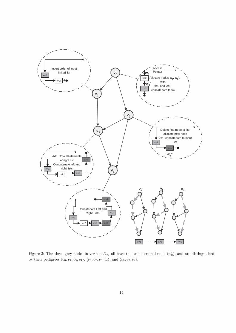
Figure 3: The three grey nodes in version Dv4 all have the same seminal node (w′0), and are distinguished

by their pedigrees 〈v0, v1, v3, v4〉, 〈v0, v2, v3, v4〉, and 〈v0, v2, v4〉.

14

identifier for a node w of the naive scheme is the pair (p(w), s(w)), where p(w) is the pedigree of w and s(w)

is the seminal node of w. We point out that a pedigree p = 〈v0, v1, . . . , vk = u〉 by itself may not uniquely

determine a node w in Du as there may be more than a single node allocated at version v0. An identifier

does determine w ∈ Du uniquely.

In figure 3 we see that version v4 has three nodes (the 1st, 3rd, and 5th nodes of the linked list) with the

same seminal node w′0. The pedigree of the 1st node in Dv4 is 〈v0, v1, v3, v4〉, the identifier of this node is

(〈v0, v1, v3, v4〉, w′0). The pedigree of the 2nd node in Dv4 is also 〈v0, v1, v3, v4〉 but it has a different seminal

node (w0 and not w′0), thus the identifier for the 2nd node in Dv4 is (〈v0, v1, v3, v4〉, w0). Similarly, we

can see that the identifiers for the 3rd, and 5th nodes of Dv4 are (〈v0, v2, v3, v4〉, w′0) and (〈v0, v2, v4〉, w

′0)

respectively. Note also that a node w ∈ Du is a seminal node of some node if and only if it was explicitly

allocated when Du has been created.

4.1 Full Path Method Emulation.

Our data structure consists of a collection of fat nodes. Each fat node corresponds to an explicit allocation

of a node by an update operation or in another words, to a seminal node of the naive scheme. For a fat

node f we denote its corresponding seminal node s(f) and for a seminal node s we denote its corresponding

fat node by f(s).10 For example, the update operations of Figure 3 perform 3 allocations (3 seminal nodes)

labeled w0, w′0, and w′′

0 , so our data structure will have 3 fat nodes, f(w0), f(w′0) and f(w′′

0 ).

The full path method represents a node of the naive scheme whose identifier is (r, s) by the pair (r, f(s)).

Therefore, every value of a pointer field in our simulation is such a representation.

A fat node f of our data structure represents all nodes of the naive scheme whose seminal node is s(f).

Recall that we denote this set of nodes by N(f). Note that N(f) may contain nodes that co-exist within

the same version and nodes that exist in different versions. A fat node contains the same fields as the

corresponding seminal node. Each of these fields, however, rather than storing a single value as in the

original node stores a dynamic table of field values in the fat node. To specify the representation of a set of

field values we need the following definitions.

Let (p = 〈v0, . . . , vk = u〉, w0) be the identifier of a node w ∈ Du. Let wk = w, wk−1, . . . , w1, wi ∈ Dvi

be the sequence of nodes such that wi ∈ Dviis derived from wi−1 ∈ Dvi−1 . This sequence exists by the

definition of a node pedigree. Let A be a field in w and let j be the maximum such that there has been

an assignment to field A in wj . The identifier of wj is (q = 〈v0, v1, . . . , vj〉, w0). We define the assignment

pedigree of a field A in node w, denoted by p(A, w), to be the pedigree of wj , i.e. q.

In the example of Figure 3 the nodes contain one pointer field (named next) and one data field (named

x). The assignment pedigree of x in the 1st node of Dv4 is simply 〈v0〉, the assignment pedigree of x in the

2nd node of Dv4 is likewise 〈v0〉, the assignment pedigree of x in the 3rd node of Dv4 is 〈v0, v2, v3〉. Pointer

fields also have assignment pedigrees. The assignment pedigree of the pointer field in the 1st node of Dv4

is 〈v0, v1〉, the assignment pedigree of the pointer field in the 2nd node of Dv4 is 〈v0, v1, v3〉, the assignment

pedigree of the pointer field of the 3rd node of Dv4 is 〈v0, v2〉, finally, the assignment pedigree of the pointer

field of the 4th node of Dv4 is 〈v2, v3, v4〉.

We call the set p(A, w) | w ∈ N(f) the set of all assignment pedigrees for field A in a fat note f , and

denote it by P (A, f). The table that represents field A in fat node f contains an entry for each assignment

pedigree in P (A, f). The value of a table entry, indexed by an assignment pedigree p, depends on the type

of the field as follows.

10Note that we use the function s() to denote the seminal node of a node w of the naive scheme, and to denote the seminal

node corresponding to a fat node f . No confusion will occur.

15

f(w 0 )

f(w 0 ' ) Assignment Pedigree Field Value

<v 0 > 1

x

next

Assignment Pedigree

<v 0 >

(<v 0 ,v 1 >,f(w 0 )) <v 0 ,v 1 >

null

(<v 2 >,f(w 0 ''))

<v 0 , v 2 , v 3 > 3

<v 0 ,v 2 >

f(w 0 '' ) Assignment Pedigree Field Value

<v 2 > 1

x

next

Assignment Pedigree

<v 2 >

(<v 0 , v 2 , v 4 > ,f(w 0 ' ) )

null

< v 2 , v 3 > 3

<v 2 , v 3 , v 4 >

Assignment Pedigree Field Value

<v 0 > 2

x

next

Assignment Pedigree Field Value

<v 0 > (<v 0 >,f(w 0 '))

<v 0 ,v 1 >

<v 0 ,v 1 ,v 3 >

null

(<v 0 ,v 2 ,v 3 >,f(w 0 '))

Field Value

Field Value

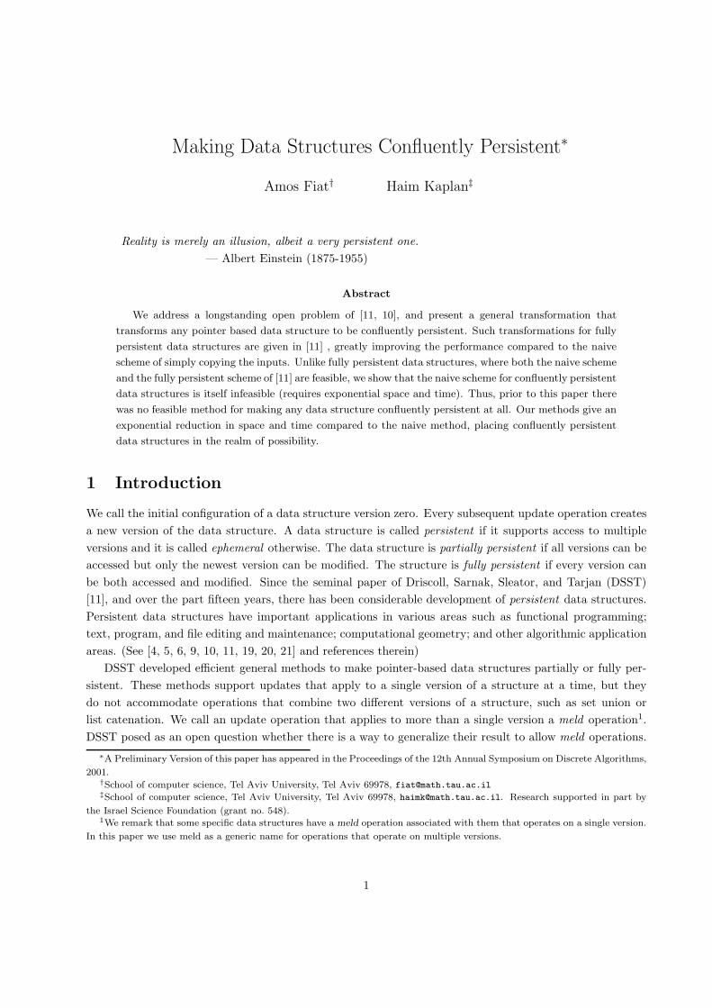
Figure 4: The fat nodes for the example of Figure 3.

16

Version Access Pointer

Dv0 (〈v0〉, f(w0))

Dv1 (〈v0, v1〉, f(w′0))

Dv2 (〈v0, v2〉, f(w′0))

Dv3 (〈v0, v1, v3〉, f(w′0))

Dv4 (〈v0, v1, v3, v4〉, f(w′0))

Table 3: Access pointers for versions v0, . . . , v4 in confluently persistent data structure of Figure 4.

1. Data fields: For the assignment pedigree p = 〈v0, v1, . . . , vj〉, let wj ∈ Dvjbe the node whose identifier

is (p, s(f)). The value stored in this entry is the value assigned to A in wj .

2. Pointer fields: For the assignment pedigree p = 〈v0, v1, . . . , vj〉, let wj ∈ Dvjbe the node whose

identifier is (p, s(f)). Consider the assignment to A in this node, this assignment is either null or a

pointer to some node w′ ∈ Dvj. If the pointer is assigned null then the value we store with p is also null.

Otherwise, the value we store with p is the pair (p′, f(s′)) where (p′, s′) is the identifier of w′ ∈ Dvj.

If A is a data field then its value in a node w ∈ N(f) is the same as its value in the node w′ ∈ N(f)

whose pedigree is p(A, w). (Note that w′ = w if there has been an assignment to A in w.) Thus the table

contains all possible values taken by A in nodes of N(f). For pointer fields however this is not the case.

The value of a pointer field in a node w ∈ N(f) is not the same as the value of the field in the node whose

pedigree is p(A, w). So our table does not contain all possible values taken by A in nodes of N(f). We will

show however that from the values stored in the table we can compute all other values.

In Figure 4 we give the fat nodes of the persistent data structure given in Figure 3. For example,

the field next has three assignments in nodes of N(f(w′0)). Thus, there are three assignment pedigrees in

P (next, f(w′0)):

1. 〈v0〉 — allocation of w′0 in version Dv0 and default assignment of null to next.

2. 〈v0, v1〉 — inverting the order of the linked list in version Dv1 and thus assigning next a new value.

The pointer is to a node whose identifier is (〈v0, v1〉, w0) so we associated the value (〈v0, v1〉, f(w0))

with 〈v0, v1〉.

3. 〈v0, v2〉 — allocating a new node, w′′0 , in version Dv2 , and assigning next to point to this new node.

The identifier for w′′0 is (〈v2〉, w

′′0 ) so we associate the value (〈v2〉, f(w′′

0 )) with 〈v0, v2〉.

You can see all three entries in the table for next in the fat node f(w′0) (Figure 4). Similarly, we give the

table for field x in f(w′0) as well as the tables for both fields in fat nodes f(w0) and f(w′′

0 ).

Consider a version v in the naive scheme. There is a set B of access pointers associated with this version.

Consider one such pointer, q ∈ B, pointing to node w ∈ Dv. The node pointed to, w, has some identifier

(p, s). The corresponding access pointer q which we store at v in our full path method data structure is the

pair (p, f(s)). (We assume that the access pointers to version v are stored in the corresponding vertex of the

version DAG.) Table 3 gives the five access pointers required for the confluently persistent data structure of

Figure 4.

17

4.2 Retrieving Field Values.

Given a pointer to a fat node f and a pedigree q such that (q, s(f)) is an identifier of some node w ∈ N(f),

we seek to obtain the value of field A in w. In order to do so, we first find the value associated with p(A, w),

the assignment pedigree of A in w, in the table representing the values of field A. By the definition of

assignment pedigree, p(A, w) is the longest prefix of q in P (A, f), so the problem reduces to finding the entry

corresponding to this prefix. We call the problem of locating the longest prefix of a pedigree q in the set

P (A, f) the pedigree maximum prefix problem.

In case A is a data field, after solving the corresponding instance of the pedigree maximum prefix problem,

we are done. The value of field A in w is simply the value associated with p(A, w). However, if A is a pointer

field then the value stored with p(A, w) may not be the value of A in w.

In case A is a pointer field the value associated with p(A, w) is either null or a pair (p, f). If this value

is null then the value of field A in w is also null. We next consider the case where this value is a pair (p, f).

Let q = 〈q0, . . . , qk〉 and let p(A, w) = 〈q0, q1, . . . , qj〉. Since the value of p(A, w) is (p, f) we know that

field A of node xj ∈ Dqjwhose identifier is (p(A, w), s(f)) was assigned a pointer to node yj whose identifier

is (p, s(f)). Since x and y are both nodes of Dqjthe last node on p must be qj .

Let xi, j ≤ i ≤ k, be the node in version Dqiwhose identifier is (〈q0, q1, . . . , qi〉, s(f)). Let yi, j ≤ i ≤ k,

be the node in version Dqiwhose identifier is (p‖〈qj+1, . . . , qi〉, s(f)). From the definition of assignment

pedigree follows that for j < i ≤ k, there is no assignment to field A in node xi ∈ Dqi. Thus, node xi ∈ Dqi

points to node yi ∈ Dqi. In particular node w = xk ∈ Dqk

points to node u = yk ∈ Dqk. So the value of

field A in w is (p ‖〈qj+1, . . . , qi〉, s(f)), where ‖ represents concatenation.

To summarize, the process of computing the value of a pointer field A in node w whose identifier is

(q, s(f)) is as follows: We search the table containing P (A, f) for the value (p, f) associated with the

assignment pedigree of A in w, p(A, w). Once we find (p, f) then the fat-node component of the value of A

in w is f . To obtain the pedigree component of the value of A in w we replace the prefix p(A, w) of q with

p. We call this transformation pedigree prefix substitution.

A Detailed Example of Traversal in a Confluently Persistent Data Structure.

Continuing the example of Figures 3 and 4 and Table 3, we now show how to traverse the linked list

y1, y2, . . . of version Dv4 . The access pointer for Dv4 , (〈v0, v1, v3, v4〉, f(w′0)), is a representation of y1. To

obtain the values of x and next for y1, we go to the fat node f(w′0) and apply the process described above.

The assignment pedigree of field x in y1, p(x, y1), is the longest prefix of 〈v0, v1, v3, v4〉 in the assign-

ment pedigree table for x stored in f(w′0). This is 〈v0〉 so the value of x in y1 is 1. The assignment

pedigree of field next in y1, p(next, y1), is 〈v0, v1〉, and the value associated with this entry in the table is

(〈v0, v1〉, f(w0)). According to the algorithm above to obtain the representation of y2 we need to replace

the prefix p(next, y1) (〈v0, v1〉) of the pedigree of y1 (〈v0, v1, v3, v4〉) with the pedigree component of the

retrieved value (〈v0, v1〉). In this case — this substitution does not change the pedigree. The representation

of y2 is therefore (〈v0, v1, v3, v4〉, f(w0)).

The assignment pedigree of field x in y2, p(x, y2), is the longest prefix of 〈v0, v1, v3, v4〉 in the assignment

pedigree table for x stored in f(w0). This is 〈v0〉 so the value of x in y2 is 2. The assignment pedi-

gree of field next in y2, p(next, y2), is 〈v0, v1, v3〉, and the value associated with this entry in the table is

(〈v0, v2, v3〉, f(w′0)). To obtain the representation of y3 we need to replace the prefix p(next, y2) (〈v0, v1, v3〉)

of the pedigree of y2 (〈v0, v1, v3, v4〉) with the pedigree component of the field value i.e. 〈v0, v2, v3〉. The

representation of y3 is therefore (〈v0, v2, v3, v4〉, f(w′0)).

The assignment pedigree of x in y3 is 〈v0, v2, v3〉, the value of x in y3 is 3. The assignment pedigree of

next in y3 is 〈v0, v2〉, the value associated with it is (〈v2〉, f(w′′0 )). After prefix substitution we obtain that

18

the representation of y4 is (〈v2, v3, v4〉, f(w′′0 )).

The assignment pedigree of x in y4 is 〈v2, v3〉, the value of x in y4 is 3. The assignment pedigree of

next in y4 is 〈v2, v3, v4〉, and the value associated with it is (〈v0, v2, v4〉, f(w′0)). After prefix substitution we

obtain that the representation of y5 is (〈v0, v2, v4〉, f(w′0)).

The assignment pedigree of x in y5 is 〈v0〉, the value of x in y5 is 1. The assignment pedigree of next in

y5 is 〈v0, v2〉, and the value associated with it is (〈v2〉, f(w′′0 )). After prefix substitution we obtain that the

value of next which is the representation of y6 is (〈v2, v4〉, f(w′′0 )).

The assignment pedigree of x in y6 is 〈v2〉, the value of x in y6 is 1. The assignment pedigree of next in

y6 is 〈v2〉, the value associated with it is null. Therefore the value of next in y6 is also null and the list ends.

4.3 Simulating updates

When we create a new version v from versions v1, . . . , vk we first consider v simply as a disjoint union of

v1, . . . , vk. To do that we initialize the set of access pointers to v to be the union of the sets of access

pointers to v1, . . . , vk after augmenting each access pointer (p, f) by adding v as the last vertex of p. Then

we continue and simulate the update operation used to produce v. We simulate traversal steps as described

above. We simulate assignments as follows.

When we assign a value N to a data field A in a node w represented by the pair (p, f) we add p to the

table associated with field A in f if it is not already there. We set the value associated with p in this table

to be N .

Assignment to a pointer field is handled in a similar way. Let (p, f) be the pair representing the node

containing pointer field A to which we want to assign a value. If the pointer should point to the node whose

identifier is (p′, s(f ′)) we add p to the table associated with A in f if it is not already there and store the

pair (p′, f ′) as the corresponding value.

4.4 Implementation and Analysis

We assume that each version is numbered uniquely and we represent a path in the version DAG by the

sequence of the numbers of the versions on the path. We represent this sequence of numbers as a linked list.

To obtain an efficient implementation of the full path method data structure we need a representation for

the tables representing field values in the fat nodes. This representation should allow to solve the pedigree

maximum prefix problem efficiently.

One possible representation is a trie which contains all assignment pedigrees in the table. Each edge

in the trie is labeled by a version number, and each path in the trie corresponds to a path in the version

DAG. The trie is organized such that it contains a path for each assignment pedigree of the corresponding

field. The value associated with an assignment pedigree is stored at the last node of the corresponding path.

The number of children of a node in such a trie is unbounded. Therefore in order to efficiently traverse a

path in the trie we could represent the children of each particular node as items of a search tree keyed by

version numbers. Using a red-black tree [12] (or any other kind of unweighted search tree data structure)

to represent the list of children of every node we can find the longest prefix of a pedigree q which is an

assignment pedigree in time O(|q| log d) where d is the maximum outdegree of a node in the version DAG11.

We can obtain a more efficient representation of the trie above by using a splay tree [22] or a biased

search tree [2] to represent the children of each node12. These types of trees allow to search for a node

11Note that the outdegree of a node in the DAG upper bounds the outdegree of a node in the trie.12When we use a biased search tree the weight we associate with each node x is the number of assignment pedigrees that

terminate at (not necessarily proper) descendants of x.

19

in time proportional to some nonnegative weight associated with it. Sleator and Tarjan in [22] describe

such an implementation of a trie using splay trees13, they call these tries lexicographic splay trees. In a

lexicographic splay tree the search for a node y within the list of children of a node x takes time proportional

to log(s(x)/s(y))+O(1) where s(z) is the number of assignment pedigrees that terminate at (not necessarily

proper) descendants of z. Thus the search times within the children lists of nodes on a path in the trie

telescope. We obtain that with this representation we can find the longest prefix of a pedigree q which is

an assignment pedigree in time O(|q| + logF) where F is the maximum number of assignment pedigrees

associated with a particular field in a particular fat node (i.e. the maximum size of a set P (A, f)). This time

bound is amortized if splay trees are used but could be made worst-case using biased search trees.

It is not hard to show that the two possible representations of the trie data structure described above also

support insertions within the same time bounds. In particular we obtain that using splay trees we can find

a field value and simulate an assignment (as shown in 4.3) in version v in O(|d(v)| + logF) amortized time,

where d(v) is the depth of version v in the version DAG. The following Theorem summarizes the properties

of the full path method.

Theorem 4.1 Using the full path method one obtains a confluently persistent emulation of an ephemeral

data structure with the following performance during an access or update operation on version v.

1. The space consumption per assignment is O(d(v)) words (each consisting of O(log(U)) bits)14

2. Simulation of a retrieval of a field value takes O(d(v) + logF) time15, where F is the number of

assignment pedigrees associated with the field at the time of the retrieval.

3. Simulation of an assignment takes O(d(v) + logF) time15, where F is the number of assignment

pedigrees associated with the field at the time of the assignment.

Remark:

1. Note that the bounds specified in Theorem 4.1 are a refinement of the bounds given in Table 1. This

is since F = O(U), and d(v) ≤ d(D) for every vertex v.

2. If we represent the tries with regular search trees at each node then the time bounds which we obtain

are O(|d(v)| log(|V |)) = O(d(D) logU) for field retrieval and assignment.

5 The Compressed Path Method

As mentioned in Section 1.2.2 the depth of u, d(u), may be much larger than the effective depth of u, e(u). In

this section we address this problem and reduce the space complexity of our data structure to O(e(u)) words

per assignment. Note that if we count bits then this implies that the space complexity of an assignment is

within a factor of O(logU) of e(u) — the bit cost lower bound of assignments at u. To do this we introduce

13An implementation using biased search trees is analogous14We could reduce the memory requirement to O(d(v) log(|V |) + log(U)) bits, which could be stored in

O(d(v) log(|V |)/ log(|U|) + 1) words. To achieve this we represent each trie in a compressed form in which unary nodes

are eliminated and edges are labeled with a sequence of version numbers. With this representation we can add a path to the

DAG by adding at most two nodes and two edges to the trie. Pointers to the new nodes added to the trie, pointers to the

new edge labels, and pointers in the value of the field (such as the pointer to the fat node for a pointer field), are of length

O(logU) bits. The labels on the new edges and paths through the DAG that are part of the value of a pointer field are of length

O(d(v) log(|V |)) bits.15The time bounds can be made worst case with an appropriate version of Biased search trees.

20

a compressed representation for path in the version DAG. This compressed representation will also be used

to reduce the time bound of retrieving a field value at version u from O(d(u) + logF) to O(e(u) + logF).

Another property of the compressed path method is that it degenerates to the fat node method of DSST

when the version DAG is a tree.

To define the compressed representation of paths we first define a level function ℓ on the vertices of

the version DAG. The root gets a level of zero. We traverse the version DAG in topological order. Let

v be a version that is created from v1, . . . , vk. Let vj be a vertex such that ℓ(vj) is maximum among

ℓ(v1), . . . , ℓ(vk). If vj is the only vertex at level ℓ(vj) among v1, . . . , vk then assign ℓ(v) = ℓ(vj). Otherwise

we set ℓ(v) = ℓ(vj) + 1.

Consider the graph induced by taking all vertices sharing some fixed value of ℓ. This is a forest of trees.

This follows because every vertex can have at most one predecessor vertex with the same ℓ value. Let F be

the family of trees induced by the ℓ function. Every edge of the DAG is either within a tree, or goes from a

version in a lower level tree to a version in a higher level tree. Therefore every path in the DAG intersects

at most one tree per level and this intersection is a contiguous subpath. See Figure 5.

Note that the function ℓ can be computed and the partition F can be maintained in an online manner

where new vertices are added to the version DAG over time.

Given a path p = 〈u0, u1, . . . , uk〉 in the DAG and a parition F of the DAG into trees, we define the

compressed representation of p, and denote it by c(p), as follows. The compressed representation is a sequence

of pairs c(p) = 〈e1 = u0, t1, e2, t2, . . . , ej , tj = uk〉 where for some i’s ei may be equal to ti, such that

1. For all 1 ≤ i ≤ j − 1, ti and ei+1 are consecutive vertices along p.

2. For all 1 ≤ m ≤ j there exists a unique T ∈ F such that the subpath of p between ei and ti (inclusive)

belongs to T , and furthermore any longer subpath p′ of p that properly contains the subpath between

ei to ti (inclusive) is not contained in T . (Note that the subpath of p from ei to ti consists of a single

vertex in case ei = ti)

The paths p that we are interested in are pedigrees, and we will refer to c(p) as a compressed pedigree. It

follows from our definitions that given a compressed representation c there is a unique path p in the DAG

such c = c(p). The following lemma bounds the length of a compressed pedigree.

Lemma 5.1 Let p be a path from the root of the DAG to u. The length of c(p) is O(e(u)).

Proof: Let R(u) be the set of paths from the root rt of the DAG to u. We prove that |c(p)| = O(log(|R(u)|)).

The lemma then follows by the definition of e(u).

What we actually prove is that the level of u, ℓ(u) ≤ log(|R(u)|), as c(p) ≤ 2ℓ(u) this implies the theorem.

This proof is by induction on ℓ(u). For u such that ℓ(u) = 0, |R(u)| = 1. This follows because if there

were ≥ 2 different paths from rt to u then u must have had two predecessors of level ≥ 0 which implies that

the level of u ≥ 1.

Consider a vertex u with ℓ(u) = i ≥ 1, one of two conditions must hold (1) it has ≥ 2 predecessors

v1, v2, . . . of level i − 1 or (2) it has exactly one predecessor of level i. In case (1) the number of paths from

rt to u is ≥ |R(v1)| + |R(v2)|. By induction, this gives |R(u)| ≥ 2ℓ(v1) + 2ℓ(v2) = 2ℓ(u) as required. In case

(2) consider the root of the tree in F containing u. This root, ru, also has level ℓ(u) and obeys condition

(1). Thus |R(u)| ≥ |R(ru)| ≥ 2ℓ(u). 2

The key idea of the compressed path method is to modify our full path method to make use of the

compressed representation of a path rather than the path itself. The essence of this modification is to make

21

0

1

0 0

0 0

1

1

1

1

0

1

2

2

2

1 u

3 u

4 u

5 u

6 u

2 u

0

1

7 u

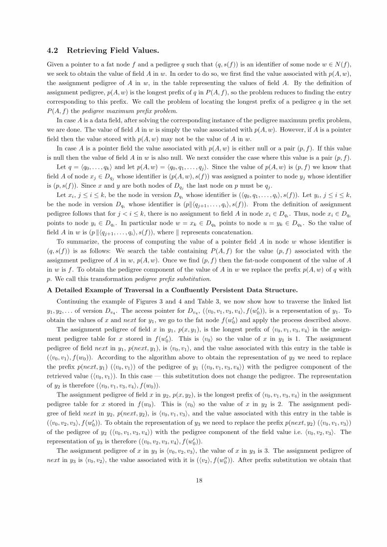
Figure 5: Computing the level function and the partition into trees. The numerical values 0,1,2 are the

levels. A typical path through the DAG consists of subpaths, each of which is entirely contained within one

of the trees interspersed with single edges from one tree to the next. The compressed representation is the

sequence of pairs of entry and exit vertices in each such tree. The path p = 〈u1, u2, . . . , u7〉 has a compressed

representation c(p) = 〈u1, u3, u4, u6, u7, u7〉.

22

Search Path q

1 e

2 e

3 e

4 e

1 t

2 t

3 t

4 t

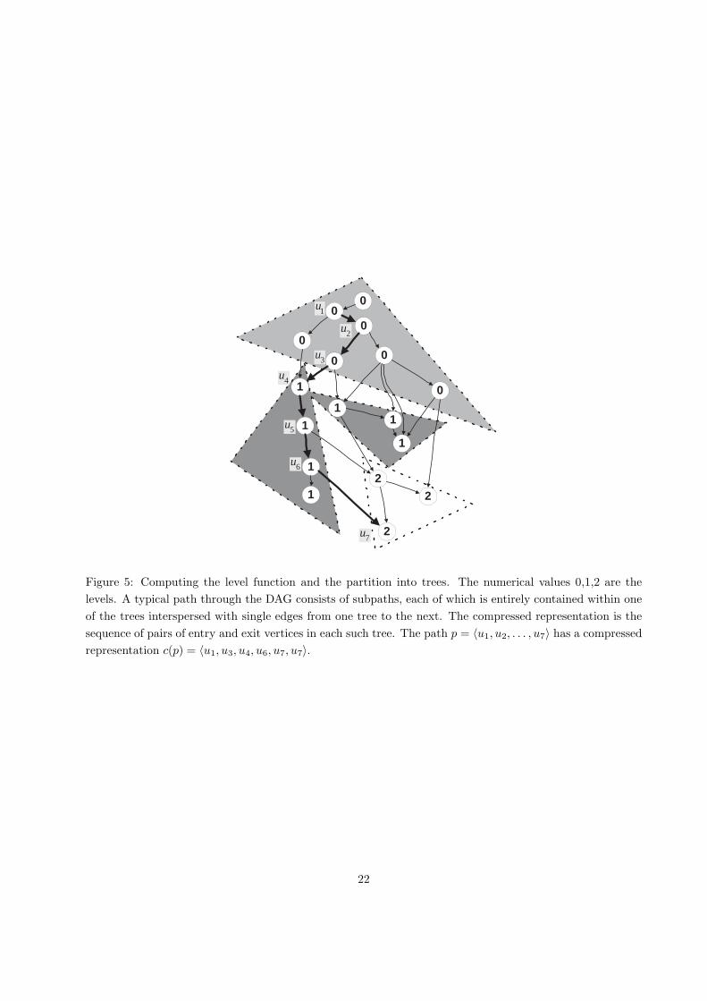
Figure 6: Given a fat node f and a compressed node pedigree (c(q) = 〈e1, t1, e2, t2, e3, t3, e4, t4〉) we want to

find the the value of the field in the node whose identifier is (q, s(f)).

our simulation use (c(q), f) rather than (q, f) to represent a node whose identifier is (q, s(f)). This requires

to represent the tables storing field values such that we can solve the pedigree maximum prefix problem

efficiently using the compressed pedigree of the node that we traverse, and the compressed assignment

pedigrees of the field.

For pointer fields we also change the values associated with assignment pedigrees in the corresponding

tables. Let p = 〈v0, v1, . . . , vj〉 be an assignment pedigree of some pointer field A in fat node f . Let wj ∈ Dvj

be the node whose identifier is (p, s(f)). Consider the assignment to A in this node, the assigned value is

either null or a pointer to some node w′ ∈ Dvj. If the pointer is assigned null then the value we store with

p is also null. Otherwise, the value we store with p is the pair (c(p′), f(s′)) where (p′, s′) is the identifier of

w′ ∈ Dvj.

In the full path method, to retrieve a value of a pointer field from node w we use the value associated

with the assignment pedigree of the field to substitute for a prefix in the pedigree of w. In the compressed

path method we have to be able to perform pedigree prefix substitution using compressed pedigrees.

Note that in the compressed path method, access pointers make use of compressed pedigrees rather than

pedigrees in the full path method. Specifically, each access pointer is a representation (c(p), f) of a node w

to which a corresponding access pointer points to in the naive scheme.

5.1 Retrieving field values

Analogously to our approach in the full path method, our goal is that given a pointer to a fat node f and a

compressed pedigree c(q) such that (q, s(f)) is an identifier of some node w ∈ N(f), we seek to obtain the

value of a field A in w. In order to do so, we want to find the value associated with p(A, w), the assignment

pedigree of A in w. For that we need to solve the pedigree maximum prefix problem, using c(q) rather than

23

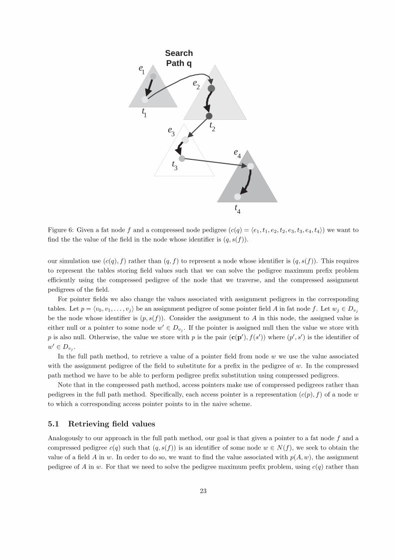
1 e

Assignment Pedigree 1

Assignment Pedigree 2

1 e

1 t

2 e

2 ' t

Assignment Pedigree 3

1 e

1 t

2 e

2 t

2 ' t

3 e

3 ' t

Assignment Pedigree 4

1 e

1 t

2 e

2 '' t

Assignment Pedigree 5

1 e

1 ' t

A = 3

A = 5

A = 7

A = 11

A = 13

2 e

2 ''' t

2 e

2 '' t 2 ' t

A = 3

A = 11

A = 5

Figure 7: The various assignment pedigrees for the field and a pictorial representation of the DSST data

structure for the index 〈e1, t1, e2〉.

24

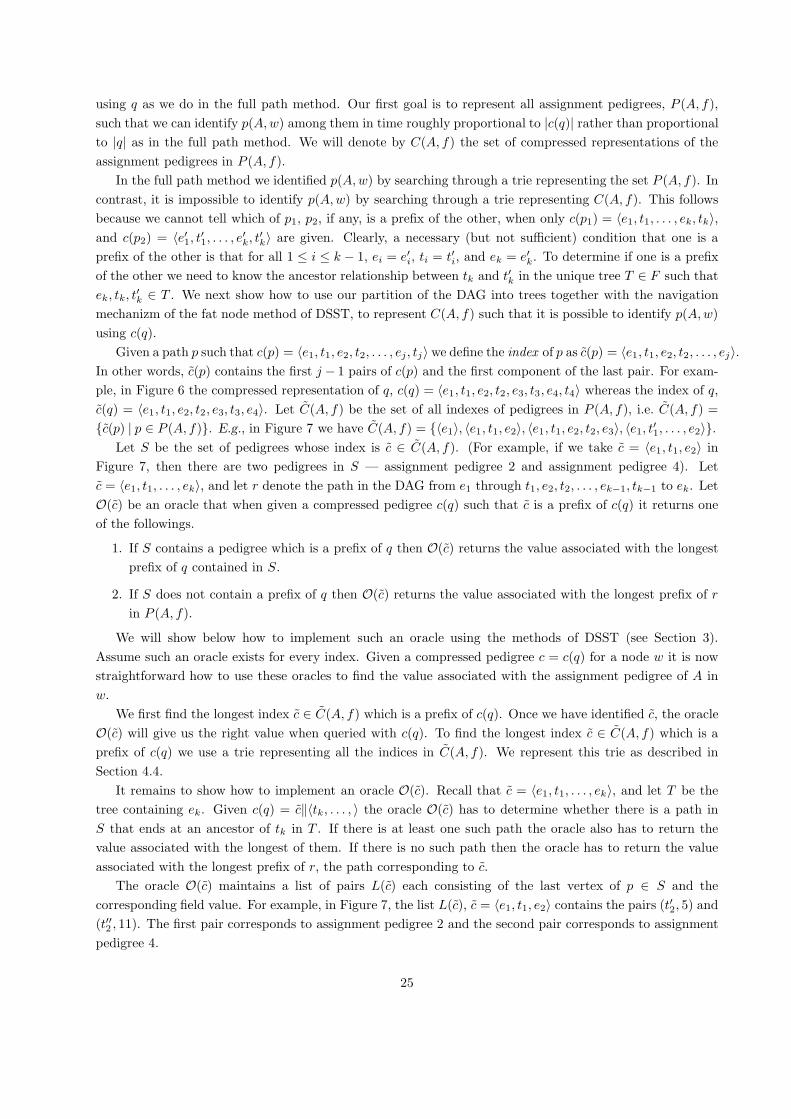
using q as we do in the full path method. Our first goal is to represent all assignment pedigrees, P (A, f),

such that we can identify p(A, w) among them in time roughly proportional to |c(q)| rather than proportional

to |q| as in the full path method. We will denote by C(A, f) the set of compressed representations of the

assignment pedigrees in P (A, f).

In the full path method we identified p(A, w) by searching through a trie representing the set P (A, f). In

contrast, it is impossible to identify p(A, w) by searching through a trie representing C(A, f). This follows

because we cannot tell which of p1, p2, if any, is a prefix of the other, when only c(p1) = 〈e1, t1, . . . , ek, tk〉,

and c(p2) = 〈e′1, t′1, . . . , e

′k, t′k〉 are given. Clearly, a necessary (but not sufficient) condition that one is a

prefix of the other is that for all 1 ≤ i ≤ k − 1, ei = e′i, ti = t′i, and ek = e′k. To determine if one is a prefix

of the other we need to know the ancestor relationship between tk and t′k in the unique tree T ∈ F such that

ek, tk, t′k ∈ T . We next show how to use our partition of the DAG into trees together with the navigation

mechanizm of the fat node method of DSST, to represent C(A, f) such that it is possible to identify p(A, w)

using c(q).

Given a path p such that c(p) = 〈e1, t1, e2, t2, . . . , ej, tj〉 we define the index of p as c(p) = 〈e1, t1, e2, t2, . . . , ej〉.

In other words, c(p) contains the first j − 1 pairs of c(p) and the first component of the last pair. For exam-

ple, in Figure 6 the compressed representation of q, c(q) = 〈e1, t1, e2, t2, e3, t3, e4, t4〉 whereas the index of q,

c(q) = 〈e1, t1, e2, t2, e3, t3, e4〉. Let C(A, f) be the set of all indexes of pedigrees in P (A, f), i.e. C(A, f) =

c(p) | p ∈ P (A, f). E.g., in Figure 7 we have C(A, f) = 〈e1〉, 〈e1, t1, e2〉, 〈e1, t1, e2, t2, e3〉, 〈e1, t′1, . . . , e2〉.

Let S be the set of pedigrees whose index is c ∈ C(A, f). (For example, if we take c = 〈e1, t1, e2〉 in

Figure 7, then there are two pedigrees in S — assignment pedigree 2 and assignment pedigree 4). Let

c = 〈e1, t1, . . . , ek〉, and let r denote the path in the DAG from e1 through t1, e2, t2, . . . , ek−1, tk−1 to ek. Let

O(c) be an oracle that when given a compressed pedigree c(q) such that c is a prefix of c(q) it returns one

of the followings.

1. If S contains a pedigree which is a prefix of q then O(c) returns the value associated with the longest

prefix of q contained in S.

2. If S does not contain a prefix of q then O(c) returns the value associated with the longest prefix of r

in P (A, f).

We will show below how to implement such an oracle using the methods of DSST (see Section 3).

Assume such an oracle exists for every index. Given a compressed pedigree c = c(q) for a node w it is now

straightforward how to use these oracles to find the value associated with the assignment pedigree of A in

w.

We first find the longest index c ∈ C(A, f) which is a prefix of c(q). Once we have identified c, the oracle

O(c) will give us the right value when queried with c(q). To find the longest index c ∈ C(A, f) which is a

prefix of c(q) we use a trie representing all the indices in C(A, f). We represent this trie as described in

Section 4.4.

It remains to show how to implement an oracle O(c). Recall that c = 〈e1, t1, . . . , ek〉, and let T be the

tree containing ek. Given c(q) = c‖〈tk, . . . , 〉 the oracle O(c) has to determine whether there is a path in

S that ends at an ancestor of tk in T . If there is at least one such path the oracle also has to return the

value associated with the longest of them. If there is no such path then the oracle has to return the value

associated with the longest prefix of r, the path corresponding to c.

The oracle O(c) maintains a list of pairs L(c) each consisting of the last vertex of p ∈ S and the

corresponding field value. For example, in Figure 7, the list L(c), c = 〈e1, t1, e2〉 contains the pairs (t′2, 5) and

(t′′2 , 11). The first pair corresponds to assignment pedigree 2 and the second pair corresponds to assignment

pedigree 4.

25

If r ∈ S then L(c) contains a pair whose first component is ek, the last version on c. Otherwise we add

to L(c) a pair, (ek, N), where N is the value associated with the longest prefix of r in P (A, f). Such a prefix

is guaranteed to exist as the field A gets an initial value whenever a node is allocated. To give an example,

in Figure 7, for c = 〈e1, t1, e2〉, we add a pair (e2, 3) to L(c) since 3 is the value associated with assignment

pedigree 1, the longest prefix of the path defined by c in P (A, f).

Let T be the tree containing ek – the last version of c, and let tk ∈ T be the exit version of the query

path c(q) from T . The oracle O(c), has to return the value associated with the version in L(c) which is the

closest ancestor of tk. This is exactly the problem DSST solve in order to find the right field value in their

fully persistent data structures (see Section 3).

We represent each list L(c) as DSST represent the set of field values in each field of their fat nodes. For

each tree T ∈ F we maintain a linear order consistent with a preorder traversal of T as DSST do for their

version tree. Note that this linear order is maintained once per tree T but we use it for all lists L(c) such

that the last vertex of c is in T . The pairs in every list L(c) are ordered according to the linear order on T –

the tree that contains the last vertex w on c.16 We shall refer to such an implementation of the oracle O(c)

as a DSST structure.

Example. We now demonstrate the process of retrieving a field value using Figures 6 and 7. Suppose we

want to find the value associated with field A in a node whose identifier is (q, s(f)) where q is shown in

Figure 6 and c(q) = 〈e1, t1, e2, t2, e3, t3, e4, t4〉. The assignment pedigrees of field A in f are shown in Figure

7. The first stage of the algorithm is to identify the longest prefix in C(A, f) that is a prefix of c(q). In our

example this index is c = 〈e1, t1, e2, t2, e3〉.

Among all the assignment pedigrees of field A in f only assignment pedigree 3 has the index c. Therefore

the list of values maintained by the oracle associated with c, L(c), contains the pair (t′3, 7). Since the path p

corresponding to c, is not an assignment pedigree of field A (i.e., , p 6∈ P (A, f)), the list L(c) also contains

the pair (e3, 5). This is because 5 is the value associated with assignment pedigree 2 which is the longest

prefix in P (A, f) of the path p.

Upon receiving the query c(q) and assuming that t3 shown in Figure 6 is not a descendant of t′3 shown

in Figure 7, the oracle returns the value 5 associated with e3. This is because among the versions e3 and t′3that have values associated with them in L(c), e3 is the only one that is an ancestor of t3 – the exit version

of c(q) from T . The value associated with assignment pedigree 2 is indeed the right value of field A in the

node identified by (q, s(f)).

Retrieving values of Pointer Fields. As in the full path method in order to find the value of a data

field A in node w it suffices to solve an instance of the pedigree maximum prefix problem in order to find

the value associated with p(A, w), which is also the value of field A in w. However for a pointer field finding

the value associated with p(A, w) is only the first stage. Once we have this value we need to replace a prefix

of the pedigree of w to obtain the pedigree of the target node.

Let (q = 〈q1, . . . , qk〉, s(f)) be the identifier of w, and let the assignment pedigree of pointer field A in

w be p(A, w) = 〈q0, q1, . . . , qj〉. The value stored with the assignment pedigree p(A, w) is a representation

(c(p), f ′) of a node (identified by (p, s(f ′))) to which the node (p(A, w), s(f)) points. A shown in Section 4 the

representation of the node to which field A in w points is (q′, f ′) where q′ is obtained from q by substituting p

for p(A, w) in q. Here we have to show how to obtain c(q′) from c(q) and c(p). Let c(q) = 〈e1, t1, . . . , em, tm〉

and let c(p) = 〈e′1, t′1, . . . , e

′n, t′n〉.

Recall that p, and p(A, w) must end at the same vertex as they are pedigrees of two nodes at the same

16DSST in fact maintain some additional version-value pairs in L(c) in order to return the right value. Each assignment

pedigree may add to L(c) at most two version-value pairs. For the precise details see DSST.

26

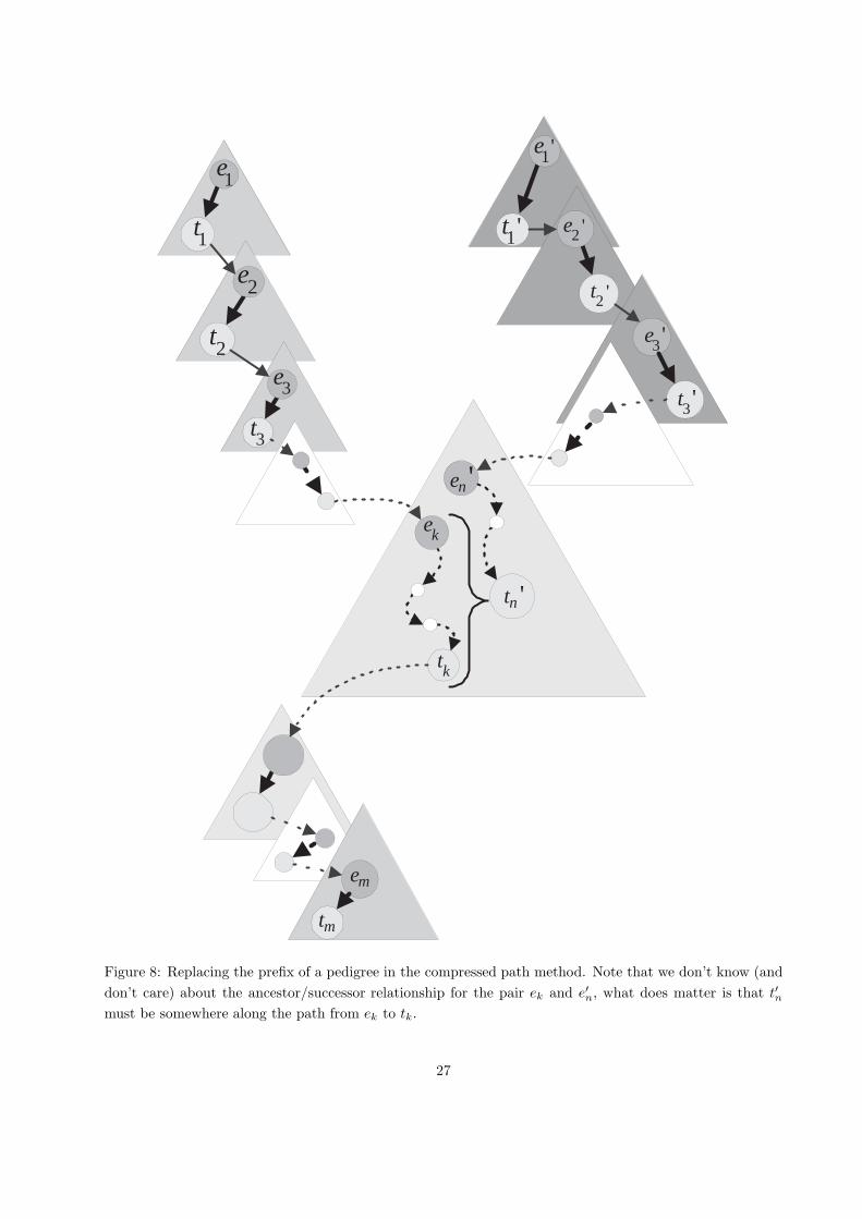
1 e

1 t

2 e

2 t

3 e

3 t

k e

' n e

' n t

k t

1 ' e

1 ' t 2 ' e

2 ' t

3 ' e

3 ' t

m t

m e

Figure 8: Replacing the prefix of a pedigree in the compressed path method. Note that we don’t know (and

don’t care) about the ancestor/successor relationship for the pair ek and e′n, what does matter is that t′nmust be somewhere along the path from ek to tk.

27

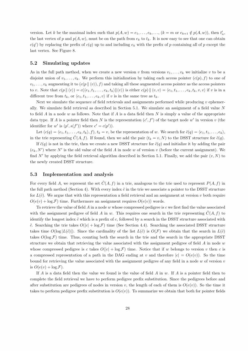
version. Let k be the maximal index such that p(A, w) = e1, . . . , ek, . . ., (k = m or ek+1 /∈ p(A, w)), then t′n,

the last vertex of p and p(A, w), must be on the path from ek to tk. It is now easy to see that one can obtain

c(q′) by replacing the prefix of c(q) up to and including ek with the prefix of p containing all of p except the

last vertex. See Figure 8.

5.2 Simulating updates

As in the full path method, when we create a new version v from versions v1, . . . , vk we initialize v to be a

disjoint union of v1, . . . , vk. We perform this initialization by taking each access pointer (c(p), f) to one of

v1, . . . , vk augmenting it to (c(p ‖ 〈v〉), f) and taking all these augmented access pointer as the access pointers

to v. Note that c(p ‖ 〈v〉) = c(〈e1, t1, . . . , ek, tk〉‖〈v〉) is either c(p) ‖ 〈v, v〉 = 〈e1, t1, . . . , ek, tk, v, v〉 if v is in a

different tree from tk, or 〈e1, t1, . . . , ek, v〉 if v is in the same tree as tk.

Next we simulate the sequence of field retrievals and assignments performed while producing v ephemer-

ally. We simulate field retrieval as described in Section 5.1. We simulate an assignment of a field value N

to field A in a node w as follows. Note that if A is a data field then N is simply a value of the appropriate

data type. If A is a pointer field then N is the representation (c′, f ′) of the target node w′ in version v (the

identifier for w′ is (p′, s(f ′)) where c′ = c(p′)).

Let (c(q) = 〈e1, t1, . . . , ek, tk〉, f), tk = v, be the representation of w. We search for c(q) = 〈e1, t1, . . . , ek〉,

in the trie representing C(A, f). If found, then we add the pair (tk = v, N) to the DSST structure for c(q).

If c(q) is not in the trie, then we create a new DSST structure for c(q) and initialize it by adding the pair

(ek, N ′) where N ′ is the old value of the field A in node w of version v (before the current assignment). We

find N ′ by applying the field retrieval algorithm described in Section 5.1. Finally, we add the pair (v, N) to

the newly created DSST structure.

5.3 Implementation and analysis

For every field A, we represent the set C(A, f) in a trie, analogous to the trie used to represent P (A, f) in

the full path method (Section 4). With every index c in the trie we associate a pointer to the DSST structure

for L(c). We argue that with this representation a field retrieval and an assignment at version v both require

O(e(v) + logF) time. Furthermore an assignment requires O(e(v)) words.

To retrieve the value of field A in a node w whose compressed pedigree is c we first find the value associated

with the assignment pedigree of field A in w. This requires one search in the trie representing C(A, f) to

identify the longest index c which is a prefix of c, followed by a search in the DSST structure associated with

c. Searching the trie takes O(|c| + logF) time (See Section 4.4). Searching the associated DSST structure

takes time O(log |L(c)|). Since the cardinality of the list L(c) is O(F) we obtain that the search in L(c)

takes O(logF) time. Thus, counting both the search in the trie and the search in the appropriate DSST

structure we obtain that retrieving the value associated with the assignment pedigree of field A in node w

whose compressed pedigree is c takes O(|c| + logF) time. Notice that if w belongs to version v then c is

a compressed representation of a path in the DAG ending at v and therefore |c| = O(e(v)). So the time

bound for retrieving the value associated with the assignment pedigree of any field in a node w of version v

is O(e(v) + logF).

If A is a data field then the value we found is the value of field A in w. If A is a pointer field then to

complete the field retrieval we have to perform pedigree prefix substitution. Since the pedigrees before and

after substitution are pedigrees of nodes in version v, the length of each of them is O(e(v)). So the time it

takes to perform pedigree prefix substitution is O(e(v)). To summarize we obtain that both for pointer fields

28

and for data fields the time it takes to retrieve the value of the field in a node of version v is O(e(v)+ logF).

Next we analyze the time and space needed to simulate an assignment. Assume that we perform an

assignment of value N to field A of node w in version v. Let c = 〈e1, t1, . . . , ek, tk〉 be the compressed

pedigree of w. To simulate the assignment we first search the trie to see whether it contains c. This search

takes O(|c| + logF) = O(e(v) + logF) time. If the trie does not contain c then we add c to the trie. This

update to the trie takes O(e(v) + logF) time and O(|c|) = O(e(v)) space. If c is not in the trie then we also

have to create a new DSST structure for it and initialize it with a pair (ek, N ′) where N ′ is the old value of

the field in version v. It takes O(1) time to initialize a new DSST data structure. But to locate N ′ we use our

field retrieval algorithm so it takes O(e(v) + logF) time. Finally we have to add a pair (v, N) to the DSST

structure of c which takes O(logF) time. Summing up we obtain that assignment takes O(e(v)+logF) time

and consumes O(e(v)) space.

Theorem 5.1 Using the Compressed Path Method one obtains a confluently persistent emulation of an

ephemeral data structure with the following performance during an access or update operation on version v.

1. The space consumption per assignment is O(e(v)) words (each consisting of O(log(U)) bits17.

2. Simulation of a retrieval of a field value takes O(e(v) + logF) time18.

3. Simulation of an assignment takes O(e(v) + logF) time18.

Same remarks (similar to those following Theorem 4.1):

Remark.

1. Note that the bounds specified in Theorem 5.1 are a refinement of the bounds given in Table 1. This

is since F = O(U), and e(v) ≤ e(D) for every vertex v.

2. If we represent the tries with regular search tree at each node then the time bounds obtained are

O(|e(v)| log(|V |)) for field retrieval and assignment.

6 Hashing the Tries via Balanced Search Trees

In this section we show how to improve the running time of the full path method and the compressed path

method. We obtain an exponential speedup which comes at two costs. First, we have to use randomization so

we obtain a data structure that encodes correctly the collection versions with very high probability. Second,

the space consumption of the improved data structures increase. Recall that the full path method and the

compressed path method require O(d(v)) and O(e(v)) words of length O(log |V |) respectively per assignment.

Here we need O(d(v)) and O(e(v)) words of length O(log T ) bits per assignment, respectively. We recall

that T denotes the total number of field retrievals.19

We describe our results as if T is known in advance. When T is not known in advance we can use a

standard technique of guessing an initial T and rebuilding the whole data structure whenever T grows by a

factor of two.

The structure of this section is as follows. We start by describing a representation of sets of integer

sequences that may be of independent interest. If the sums of the integers in subsequences satisfy a particular

17As in the full path method by compressing the tries we can reduce this space requirement to O(e(v) log |V | + logU) bits.18This time bound can be made worst case with biased search trees and a worst case data structure to maintain a list subject

to order queries [1, 7] to maintain the linear orders of the trees.19This is only an increase by a constant factor if the number of field retrievals is polynomial in the number of versions.

29

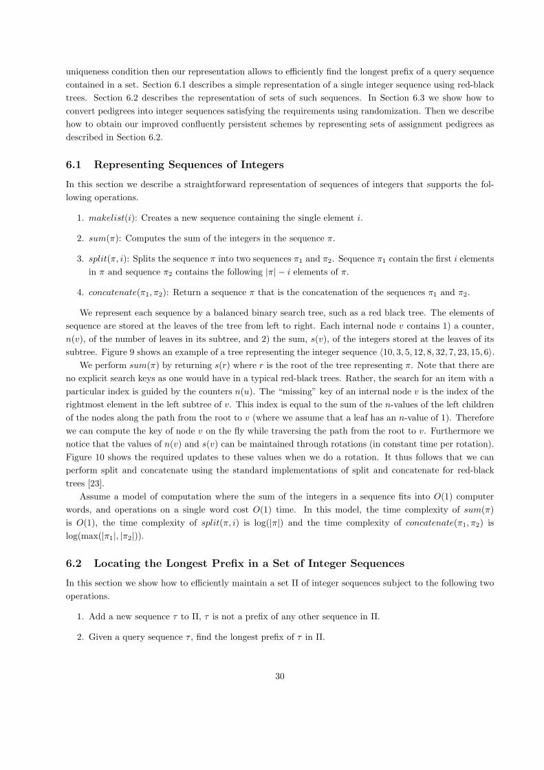
uniqueness condition then our representation allows to efficiently find the longest prefix of a query sequence

contained in a set. Section 6.1 describes a simple representation of a single integer sequence using red-black

trees. Section 6.2 describes the representation of sets of such sequences. In Section 6.3 we show how to

convert pedigrees into integer sequences satisfying the requirements using randomization. Then we describe

how to obtain our improved confluently persistent schemes by representing sets of assignment pedigrees as

described in Section 6.2.

6.1 Representing Sequences of Integers

In this section we describe a straightforward representation of sequences of integers that supports the fol-

lowing operations.

1. makelist(i): Creates a new sequence containing the single element i.

2. sum(π): Computes the sum of the integers in the sequence π.

3. split(π, i): Splits the sequence π into two sequences π1 and π2. Sequence π1 contain the first i elements

in π and sequence π2 contains the following |π| − i elements of π.

4. concatenate(π1, π2): Return a sequence π that is the concatenation of the sequences π1 and π2.

We represent each sequence by a balanced binary search tree, such as a red black tree. The elements of

sequence are stored at the leaves of the tree from left to right. Each internal node v contains 1) a counter,

n(v), of the number of leaves in its subtree, and 2) the sum, s(v), of the integers stored at the leaves of its

subtree. Figure 9 shows an example of a tree representing the integer sequence 〈10, 3, 5, 12, 8, 32, 7, 23, 15, 6〉.

We perform sum(π) by returning s(r) where r is the root of the tree representing π. Note that there are

no explicit search keys as one would have in a typical red-black trees. Rather, the search for an item with a

particular index is guided by the counters n(u). The “missing” key of an internal node v is the index of the

rightmost element in the left subtree of v. This index is equal to the sum of the n-values of the left children

of the nodes along the path from the root to v (where we assume that a leaf has an n-value of 1). Therefore

we can compute the key of node v on the fly while traversing the path from the root to v. Furthermore we

notice that the values of n(v) and s(v) can be maintained through rotations (in constant time per rotation).

Figure 10 shows the required updates to these values when we do a rotation. It thus follows that we can

perform split and concatenate using the standard implementations of split and concatenate for red-black

trees [23].

Assume a model of computation where the sum of the integers in a sequence fits into O(1) computer

words, and operations on a single word cost O(1) time. In this model, the time complexity of sum(π)

is O(1), the time complexity of split(π, i) is log(|π|) and the time complexity of concatenate(π1, π2) is

log(max(|π1|, |π2|)).

6.2 Locating the Longest Prefix in a Set of Integer Sequences

In this section we show how to efficiently maintain a set Π of integer sequences subject to the following two

operations.

1. Add a new sequence τ to Π, τ is not a prefix of any other sequence in Π.

2. Given a query sequence τ , find the longest prefix of τ in Π.

30

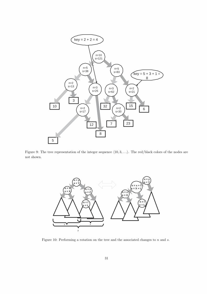
n=2 s=17

n=2 s=30

3

10

5

12

8

32

7 23

15 6

n=10 s=121

n=5 s=38

n=2 s=13 n=3

s=25

n=5 s=83

n=3 s=62

n=2 s=21

key = 5 + 3 + 1 = 8

key = 2 + 2 = 4

Figure 9: The tree representation of the integer sequence 〈10, 3, . . .〉. The red/black colors of the nodes are

not shown.

n = y s = Y

n = z s = Z

n = x s = X

n = l s = L

n = y s = Y

n = x + l s = X + L

n = x s = X

n = l s = L

y

x z

Figure 10: Performing a rotation on the tree and the associated changes to n and s.

31

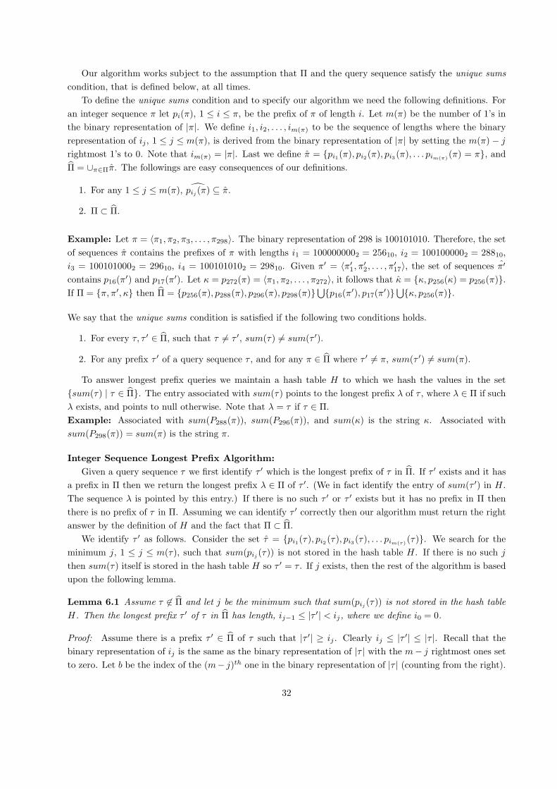
Our algorithm works subject to the assumption that Π and the query sequence satisfy the unique sums

condition, that is defined below, at all times.

To define the unique sums condition and to specify our algorithm we need the following definitions. For

an integer sequence π let pi(π), 1 ≤ i ≤ π, be the prefix of π of length i. Let m(π) be the number of 1’s in

the binary representation of |π|. We define i1, i2, . . . , im(π) to be the sequence of lengths where the binary

representation of ij, 1 ≤ j ≤ m(π), is derived from the binary representation of |π| by setting the m(π) − j

rightmost 1’s to 0. Note that im(π) = |π|. Last we define π = pi1(π), pi2(π), pi3 (π), . . . pim(π)(π) = π, and

Π = ∪π∈Ππ. The followings are easy consequences of our definitions.

1. For any 1 ≤ j ≤ m(π), pij(π) ⊆ π.

2. Π ⊂ Π.

Example: Let π = 〈π1, π2, π3, . . . , π298〉. The binary representation of 298 is 100101010. Therefore, the set

of sequences π contains the prefixes of π with lengths i1 = 1000000002 = 25610, i2 = 1001000002 = 28810,

i3 = 1001010002 = 29610, i4 = 1001010102 = 29810. Given π′ = 〈π′1, π

′2, . . . , π

′17〉, the set of sequences π′

contains p16(π′) and p17(π

′). Let κ = p272(π) = 〈π1, π2, . . . , π272〉, it follows that κ = κ, p256(κ) = p256(π).

If Π = π, π′, κ then Π = p256(π), p288(π), p296(π), p298(π)⋃p16(π

′), p17(π′)⋃κ, p256(π).

We say that the unique sums condition is satisfied if the following two conditions holds.

1. For every τ, τ ′ ∈ Π, such that τ 6= τ ′, sum(τ) 6= sum(τ ′).

2. For any prefix τ ′ of a query sequence τ , and for any π ∈ Π where τ ′ 6= π, sum(τ ′) 6= sum(π).

To answer longest prefix queries we maintain a hash table H to which we hash the values in the set

sum(τ) | τ ∈ Π. The entry associated with sum(τ) points to the longest prefix λ of τ , where λ ∈ Π if such

λ exists, and points to null otherwise. Note that λ = τ if τ ∈ Π.

Example: Associated with sum(P288(π)), sum(P296(π)), and sum(κ) is the string κ. Associated with

sum(P298(π)) = sum(π) is the string π.

Integer Sequence Longest Prefix Algorithm:

Given a query sequence τ we first identify τ ′ which is the longest prefix of τ in Π. If τ ′ exists and it has

a prefix in Π then we return the longest prefix λ ∈ Π of τ ′. (We in fact identify the entry of sum(τ ′) in H .

The sequence λ is pointed by this entry.) If there is no such τ ′ or τ ′ exists but it has no prefix in Π then

there is no prefix of τ in Π. Assuming we can identify τ ′ correctly then our algorithm must return the right

answer by the definition of H and the fact that Π ⊂ Π.

We identify τ ′ as follows. Consider the set τ = pi1(τ), pi2 (τ), pi3 (τ), . . . pim(τ)(τ). We search for the

minimum j, 1 ≤ j ≤ m(τ), such that sum(pij(τ)) is not stored in the hash table H . If there is no such j

then sum(τ) itself is stored in the hash table H so τ ′ = τ . If j exists, then the rest of the algorithm is based

upon the following lemma.

Lemma 6.1 Assume τ 6∈ Π and let j be the minimum such that sum(pij(τ)) is not stored in the hash table

H. Then the longest prefix τ ′ of τ in Π has length, ij−1 ≤ |τ ′| < ij, where we define i0 = 0.

Proof: Assume there is a prefix τ ′ ∈ Π of τ such that |τ ′| ≥ ij . Clearly ij ≤ |τ ′| ≤ |τ |. Recall that the

binary representation of ij is the same as the binary representation of |τ | with the m− j rightmost ones set

to zero. Let b be the index of the (m− j)th one in the binary representation of |τ | (counting from the right).

32

It follows that the binary representation of ij is of the form α‖0b whereas the binary representation of τ is of

the form α‖β, |β| = b. As ij ≤ |τ ′| < |τ |, the binary representation of |τ ′| must be of the form α‖γ, |γ| = b,

where 0 ≤ γ ≤ β. Therefore, Pij(τ) = Pij

(τ ′) ∈ τ ′ ⊂ Π, so sum(pij(τ)) ∈ H , contradicting the definition of

j. 2

By lemma 6.1 we now know that the longest prefix τ ′ of τ in Π is such that |τ ′| < ij . Let k be the integer

such that ij − ij−1 = 2k (define i0 = 0 if j = 1). We identify τ ′ using the following procedure.

“Binary Search” Procedure:

1. Set δ = 2k−1.

2. for ρ = k − 1 downto 1:

• If sum(pij−1+δ(τ)) is in H set δ = δ + 2ρ−1, otherwise δ = δ − 2ρ−1.

3. If sum(pij−1+δ(τ)) is in H return δ. Otherwise return δ − 1.

The following lemma shows that the binary search procedure above ends with the maximum 0 ≤ δ < 2k

such that sum(pij−1+δ(τ)) is stored in the hash table H .

Lemma 6.2 At the end of the “binary search” procedure defined above, the longest prefix of τ in Π, (whose

length is < ij), is pij−1+δ(τ).

Proof: We prove by induction that the following invariant holds.

Invariant 6.1 Before each iteration of the loop defined in step (2) of the “binary search” procedure above

and before step (3) we are guaranteed that the length of the longest prefix τ ′ of τ in Π satisfies ij−1 +δ−2ρ ≤

|τ ′| ≤ ij−1 + δ + 2ρ − 1. (We assume ρ = 0 before step (3).)

From this invariant and the definition of step (3) the lemma follows since we know that pij−1 (τ) ∈ Π.

The invariant holds before the first iteration of the loop defined by step (2) since we know that pij−1 (τ) ∈ Π

and pij(τ) /∈ Π, so from lemma 6.1 we know that the longest prefix of τ in π has length < ij and ≥ ij−1.

It is straightforward to establish the induction step using the following two observations:

1. The unique sums condition implies that if sum(Pr(τ)) is in H , then Pr(τ) is in Π, and the longest

prefix of τ in Π has length ≥ r.

2. In general, it is not true that if sum(Pr(τ)) is not in H then neither is sum(Pr′(τ)) for r′ > r. This is the

reason we place the “binary search” in quotation marks. However, a slightly weaker statement is true

and suffices to establish the induction step. If sum(Pr(τ)) is not in H , and the binary representation

of r has b low order zeros then we know that for every r′ in the range r ≤ r′ ≤ r + 2b − 1, sum(Pr′(τ))

is not in H . This follows from the definition of Π.

2

The correctness of our query algorithm stated in the following theorem now follows from the definition

of H , Lemma 6.1, and Lemma 6.2.

Theorem 6.1 For any τ and Π satisfying the unique sums condition, the integer sequence longest prefix

algorithm returns the longest prefix of τ in Π.

33

6.2.1 Adding a Sequence to Π.

To add a new sequence τ to Π, we insert the values sum(τ ′), τ ′ ∈ τ , to the table H , if they are not already

there. When adding a new entry τ ′ to H , we compute (using the query algorithm described above) the

longest prefix of τ ′ in Π, and store a pointer to a representation of this sequence.

Note that τ is not a prefix of any previous sequence is Π, by assumption, so the addition of τ does not

change the longest prefix (in Π) for any sequence in Π.

6.2.2 Implementation and Analysis.

We assume that each integer sequence is represented using a binary search tree as described in Section

6.1, where each sum of a subsequences fits into O(1) computer words. We also assume that the hash table

containing the sums of the sequences in Π is maintained using Dynamic Perfect Hashing [8]. Dynamic Perfect

Hashing allows to test whether a particular sum is in the table in O(1) worst-case time and to insert a new

sum into the table in O(1) amortized expected time. The size of the table is proportional to the number of

elements in it that is O(Π).

To find the longest prefix in Π of a query sequence τ we compute O(log |τ |) sums of sequences in τ and

another O(log |τ |) sums of sequences considered in the binary search phase. All these sequences are prefixes

of τ so we can compute the sum of each such sequence by splitting τ at the appropriate length. Thus

the computation of each such sum takes O(log |τ |) time, and the computation of all O(log |τ |) sums takes

O(log2(|τ |)) time. Probing the hash table for each sum takes O(1) time so the total query time is dominated

by the computation of the sums and takes O(log2(|τ |)) worst case time.

To insert a new sequence, τ , into Π, we need to repeat the following for each of the O(log |τ |) sequences

in τ ′ ∈ τ .

1. Compute sum(τ ′), this takes time O(log |τ |) as we need to split the tree of τ at the appropriate length

(|τ ′|).

2. If τ ′ 6= τ and sum(τ ′) /∈ H : search for the the longest prefix π ∈ Π of τ ′, this takes time O(log2(|τ ′|)).

In total, this time required to insert τ into Π is O(log3(|τ |)). This time bound is expected and amortized

since we use dynamic perfect hashing.

Remark. At the cost of a factor of O(log Π) in the time per query and the time per insertion we can

avoid using dynamic perfect hashing, and use some kind of a balanced search tree to represent the set

sum(π) | π ∈ Π. All time bounds with this implementation are worst-case.

6.3 Speeding up the Full Path Method and the Compressed Path Method via

Randomization

In this section we show how to use our representation for integer sequences from Section 6.2 to speed

up both the full path method and the compressed path method. The algorithm which we describe is

randomized and simulates retrieval and assignment in time polylogarithmic in d(D) for the full path method

and polylogarithmic in e(D) for the compressed path method. Note that to achieve such bound we need to

solve the pedigree maximum prefix problem without traversing the pedigree itself. The key idea is to map

pedigrees into integer sequences which satisfy the unique sums condition with high probability. Then we

use our representation from Section 6.2 to represent the pedigrees in P (A, f) in the full path method or the

indices in C(A, f) in the compressed path method. We first describe the details of applying this idea to the

full path method.

34

To map pedigrees into integer sequences that satisfy the unique sums condition we randomly choose for

every version v in the DAG a large random number r(v) ∈ 0, . . . , R. We map a pedigree q = 〈q0, q1, . . . , qj〉

to the integer sequence r(p) = 〈r(q0), r(q1), . . . , r(qj)〉. We call r(p) the randomized pedigree corresponding

to p. The following lemma shows that if R is large enough then the unique sums condition holds with respect

to all pedigrees accessed during the computation.

Lemma 6.3 Let P be the set of all pedigrees accessed during the computation and their prefixes. Let r(P)

be the corresponding set of integer sequences. If R = Ω(|P|3) then r(P) satisfies the unique sums condition

with probability O( 1|P|).

Proof: The probability that any two particular distinct pedigrees have random pedigrees with the same

sum is 1/R. Therefore the probability that at least one of the |P| randomized pedigrees accessed during the

computation will have the same sum is at most(|P|2

)1R

and the lemma follows. 2

Notice that if T is the number of field retrievals then |P| = O(T ∗ |V |) = O(T 2). Therefore to guarantee

the unique sums condition with high probability it suffices to use random integers of O(log T ) bits.

To speed up the full path method we modify it to use randomized pedigrees rather than the pedigrees

themselves. We represent each randomized pedigree as in Section 6.1 and use the pair (r(q), f) to represent

a node whose identifier is (q, s(f)). We define R(A, f) = r(p) | p ∈ P (A, f) and represent P (A, f) by a

hash table storing the set of sequences R(A, f) as described in Section 6.2.

Recall that the hash table representing R(A, f) contains an entry for each integer sum(π) where π ∈R(A, f). The entry of sum(π), π ∈ R(A, f) stores the longest prefix λ of π in R(A, f). Let p be the

assignment pedigree that corresponds to λ in P (A, f). If A is a data field we store with λ the value of A

in the node (p, s(f)). If A is a pointer field than we store with λ the representation (r(p′), f ′) of the node

whose address is stored in field A of the node (p, s(f)).

Let w be a node represented by the pair (q, f). Recall that in order to retrieve a value of a field A in

the node w we solve an instance of the pedigree maximum prefix problem to locate the longest prefix of

q in the set P (A, f). To solve the pedigree maximum prefix problem with our modified data structure we

use the integer sequence longest prefix algorithm of Section 6.2. Using this algorithm we locate the longest

prefix of the integer sequence r(q) in R(A, f). This prefix is the integer sequence which corresponds to the

assignment pedigree p(A, w).

If A is a data field once we find r(p(A, w)) then the value associated with it is the value of field A in

w. However if A is a pointer field then to obtain the representation of the target node we need to perform

pedigree prefix substitution. The value associated with r(p(A, w)) is a pair (r(p′), f). To obtain the value

of A in w we need to replace r(p(A, w)) by r(p′) in r(q) (the randomized pedigree of w).

We can perform pedigree prefix substitution by performing (r1, r2) = split(r(q), i) where i = |r(p(A, w))|

and concatenating r(p′) to r2. This however destroys r(p′) which has to stay intact in the representation of

R(A, f) and maybe in other places in our data structure. On the other hand, copying r(p′) entirely before

the concatenation would take Ω(|r(p′)|) time and does not improve our original full path method.

Using confluently persistent red/black trees.

To overcome this difficulty and support pedigree prefix substitution efficiently we use confluently persis-

tent red-black trees to represent the randomized pedigrees. We make red-black trees persistent using the

path copying method described in DSST. According to this method we perform split and concatenation as

we would have in a non-persistent red-black tree except that we duplicate any node which changes during

the operation. Recall that while splitting or concatenating red-black trees only O(log k) of the nodes change

35

where k is the number of leaves of the tree. Therefore by path copying we obtain confluently persistent

red-black trees such that each split or concatenate operation runs in time logarithmic in the size of the tree.

By using persistent red-black trees to represent pedigrees and performing pedigree prefix substitution via

splitting and concatenating the corresponding trees we obtain that the time required for pedigree prefix sub-

stitution is O(log |V |) (The maximum length of a pedigree is |V |). However each pedigree prefix substitution

also requires O(log |V |) new nodes. This seemingly makes the space utilization of our data structure depend

not only on the number of assignments but also on the number of retrievals of values of pointer fields.

Improving the space required for traversal.

A pointer retrieval requires O(log |V |) space for path copying. This space is allocated to construct the

representation the target node, say w. Notice that if the representation of w (or the representation of any

other node obtained by splitting and concatenating pieces of the pedigree of w) is not used as the value of

a subsequent assignment to a pointer field, then when we finish the update operation we can free the nodes

allocated specifically for the representation of w.

In general, we can classify each node allocated while retrieving the value of a pointer field as either

temporary or permanent . We say that a node allocated during a retrieval of a pointer field is permanent if

it is used in the representation of a node that is the target of a subsequent assignment into a pointer field. All

other nodes allocated during retrievals of pointer fields are classified as temporary. We can release temporary

nodes when the update operation is over and the new version is complete. This without damaging the new

or any already existing version. We associate each permanent node with an assignment operation that use

it in the representation of its value, and charge that node to this assignment.

Keeping track of which nodes are permanent and which are temporary is a nontrivial task. When we

are not in middle of an update operation then permanent pedigree-nodes are those pedigree-nodes that are

either reachable from one of our fat nodes (and the tables representing its fields), or nodes that are used to

represent an access pointer. When we are in the middle of an update operation we would also consider as

permanent those pedigree-nodes which are reachable from representations of nodes that the update operation

currently holds pointers to.

In case we implement our data structure in an environment that has a garbage collector then the garbage

collector automatically would free the temporary nodes. This is because a permanent node is always reachable

from some live variable of our program. Temporary nodes on the other hand should become unreachable

when the randomized pedigrees containing them are not needed anymore. However, while using a automatic

garbage collection mechanism may be convenient, we have no means to bound the time spent by this process.

To justify our time bounds for the data structures, we must consider all resources used including those for

garbage collection. We next consider explicit garbage collection and its associated costs.

Explicit Garbage Collection.

As before, we distinguish between allocations of fat nodes (which are never released) and allocations of

nodes required for path copying when retrieving values of pointer fields.

While performing an update operation generating a new version, we assume that all nodes allocated

for path copying can be easily identified when the update operation is over. We can achieve this by either

maintaining a linked list of pointers to these nodes or by allocating these nodes from a contiguous pool of

storage. When a node is allocated we mark it “temporary”20. While simulating the update operation we

maintain a list L of pointers to all randomized pedigrees that were stored as part of the representation of

target nodes of assignment operations.

20we assume each node has an additional mark bit for garbage collection purposes.

36

When the update operation is over we traverse all pedigrees in L as follows. While traversing a pedigree

we maintain a queue of nodes yet to be traversed. We start by inserting the root of the tree into the

queue. Each traversal step we extract a node z from the queue, change the mark of z from “temporary” to

“permanent” and add to the queue every child of z which is marked “temporary”.

When we finish traversing all the randomized pedigrees in L we traverse all nodes that were allocated

for path copying during the update operation and free those which are still marked “temporary”. We retain

nodes which changed their marks to “permanent”.21

To establish the correctness of this method to release temporary nodes we observe that all permanent

nodes indeed get marked by the above traversal. This follows from our use of path copying as the method

for obtaining persistent search trees. It is straightforward to prove by induction that with path copying each

newly allocated node is reachable by a path of newly allocated nodes from the roots of all the pedigrees

containing it. The node is permanent if at least one of these pedigrees is stored as part of the value of an

assignment operation.

The running time of this garbage collection procedure is proportional to the number of nodes allocated for

path copying. To see this note that each such node is added to the queue used for traversing the randomized

pedigrees in L at most once and it takes O(1) time to traverse a node. Thus this garbage collection phase

increases the overall running time of the update operation by no more than a constant factor.

Summary.

The following theorem summarizes the performance of the randomized full path method.

Theorem 6.2 Let T be the total number of field retrievals as defined in Section 1.2. The randomized full

path method gives a confluently persistent data structure with the following performance. Let v be the version

accessed or created by the operation.

1. The worst case space consumption per assignment is O(d(v) log TlogU ) words of Θ(logU) bits each.

2. The worst case time per field retrieval is O(log2(d(v)) · log TlogU ).

3. The expected amortized time for an assignment is O(log3(d(v)) · log TlogU ).

Remarks.

1. The time for assignment is “expected amortized” due to our use of dynamic perfect hashing, it is also

amortized for assignment because we may need to store more data than this time allows, we charge

the time required to store this data against the time spent on previous retrievals.

2. In addition, we require a garbage collection phase at the end of any update step. The cost of this

garbage collection is also charged to the time spent on retrieval steps during the update step.

3. With some polynomially small probability, the randomized full path method may give wrong results.

21As an alternative mechanism for garbage collection we note the following. If the nodes allocated for path copying during

the update operation are allocated from a contiguous pool of storage we can “squeeze” the permanent nodes so they occupy a

contiguous block of storage. To do so we have to change all the pointers to these permanent nodes. Pointers to permanent nodes

which are internal in all pedigrees containing them are located in other permanent nodes. Pointers to the roots of the pedigrees

in L are located in other places of the data structure which we need to keep track of. The number of such places is bounded by

the number of fields to which the update operation assigned values. After this “squeezing”, the release of temporary nodes is

trivial and does not require traversing all new nodes allocated.

37

We can apply the same technique to the compressed path method. For every field A in a fat node f

we represent each index c ∈ C(A, f) by the sequence of random integers, r(c), obtained by replacing each

version in c by its associated random integer. Then we represent the set r(c) | c ∈ C(A, f) as described in

Section 6.2. The value associated with the sequence r(c) is a list L(c) as in the compressed path method. The

following theorem summarizes the performance of the confluently persistent data structure that we obtain.

Theorem 6.3 Let T be the total number of field retrievals as defined in Section 1.2. The randomized

compressed path method gives a confluently persistent data structure with the following performance. Let v

be the version accessed or created by the operation.

1. The worst case space consumption per assignment is O(e(v) log TlogU ) words of Θ(logU) bits each.

2. The worst case time per field retrieval is O(log2(e(v)) · log TlogU ).

3. The expected amortized time for an assignment is O(log3(e(v)) · log TlogU ).

The remarks following Theorem 6.2 hold here as well.

7 Concluding remarks

We presented a general technique to transform a data structure to be confluently persistent. Our technique

uses a succinct representation of all versions whose explicit size may be exponential in the size of the version

DAG. This exponential blowup of the version size that is possible in the confluently persistent settings makes

the trivial node copying technique infeasible. It is infeasible even if we don’t care about persistence but only

want to access the final version. The techniques we present in this paper are the only feasible transformations

we are aware of that can be applied to any data structure and any set of operations.

The transformation we describe is completely oblivious to the nature of the allowed update operations

and works the same whatever the instantiation of the DAG is. This generality of our solution makes it

subject to the lower bound provided in Theorem 2.1 which shows that the space complexity of our structure

is optimal.

An interesting line for further research would be to try and classify general classes of data structures that

allow better bounds. It is at least possible that there is some transformation, that somehow adapts itself to

the actual instantiation of the DAG and beats the lower bounds given above. One interesting model that

may be worthwhile to consider is a weighted DAG where the weights on the edges reflect what percentage

of the nodes in the previous version that remain part of the data structure after the meld. A particularly

interesting case is the case of weights 1/2.

Acknowledgements

We thank the referees for their detailed comments that helped in improving our presentation.

References

[1] M. A. Bender, R. Cole, E. Demaine, M. Farach-Colton, and J. Zito. Two Simplified Algorithms for

Maintaining Order in a List. Proceedings of the 10th European Symposium on Algorithms (ESA), 2002.

[2] S. W. Bent, D. D. Sleator, and R. E. Tarjan. Biased search trees. SIAM Journal on Computing,

14(3):545–568, 1985.

38

[3] A. L. Buchsbaum and R. E. Tarjan. Confluently persistant deques via data structural bootstrapping.

J. of Algorithms, 18:513–547, 1995.

[4] B. Chazelle. How to search in history. Information and control, 64:77–99, 1985.

[5] R. Cole. Searching and storing similar lists. J. of Algorithms, 7:202–220, 1986.

[6] P. F. Dietz. Fully persistent arrays. In Proceedings of the 1989 Workshop on Algorithms and Data

Structures (WADS’89), pages 67–74. Springer, 1995. LNCS 382.

[7] P. F. Dietz and D. D. Sleator. Two algorithms for maintaining order in a list. In Proc. 19th Annual

ACM Symposium on Theory of Computing, pages 365–372. Springer, 1987.

[8] M. Dietzfelbinger, A. Karlin, K. Mehlhorn, F. Meyer auf der Heide, H. Rohnert, and R. E. Tarjan.

Dynamic perfect hashing: upper and lower bounds. SIAM J. Comput. 23, 1994, 738–761.

[9] D. P. Dobkin and J. I. Munro. Efficient uses of the past. J. of Algorithms, 6:455–465, 1985.

[10] J. Driscoll, D. Sleator, and R. Tarjan. Fully persistent lists with catenation. Journal of the ACM,

41(5):943–959, 1994.

[11] J. R. Driscoll, N. Sarnak, D. Sleator, and R. Tarjan. Making data structures persistent. J. of Computer

and System Science, 38:86–124, 1989.

[12] L. J. Guibas and R. Sedgewick. A Diochromatic Framework for Balanced Trees. In Proc. 19th Annual

Symposium on Foundations of Computer Science, 1978.

[13] H. Kaplan, C. Okasaki, and R. E. Tarjan. Simple confluently persistent catenable lists (extended

abstract). SIAM J. Comput. 30(3): 965-977, 2000.

[14] H. Kaplan and R. E. Tarjan. Purely functional, real-time deques with catenation. JACM 46(5):577-603,

1999.

[15] H. Kaplan and R. E. Tarjan. Purely functional representations of catenable sorted lists. In Proceedings

of the 28th Annual ACM Symposium on Theory of Computing, pages 202–211. ACM Press, 1996.

[16] C. Okasaki. Amortization, lazy evaluation, and persistence: Lists with catenation via lazy linking. In

Proc. 36th Symposium on Foundations of Computer Science, pages 646–654. IEEE, 1995.

[17] C. Okasaki. Purely functional data structures. PhD thesis, School of Computer Science, Carnegie Mellon

University, Pittsburgh, PA 15213, 1996.

[18] C. Okasaki. The role of lazy evaluation in amortized data structures. In Proc. of the International

Conference on Functional Programming, pages 62–72. ACM Press, 1996.

[19] M. H. Overmars. Searching in the past, parts I and II. Technical Reports RUU-CS-81-7 and RUU-CS-

81-9, Department of Computer Science, University of Utrecht, Utrecht,The Netherlands, 1981.

[20] N. Sarnak. Persistent Data Structures. PhD thesis, Dept. of Computer Science, New York University,

1986.

[21] N. Sarnak and R. E. Tarjan. Planar point location using persistent search trees. Communications of

the ACM, 29(7):669–679, 1986.

39

[22] D. Sleator and R. E. Tarjan. Self-adjusting binary search trees. Journal of the ACM, 32:652–686, 1985.

[23] R. E. Tarjan. Data Structures and Network Algorithms. SIAM CBMS 44, 1983.

40