Make slide with no dummies, add time dummy, then state dummy, then interaction term.

Make slide with no dummies, add time dummy, then state

dummy, then interaction term

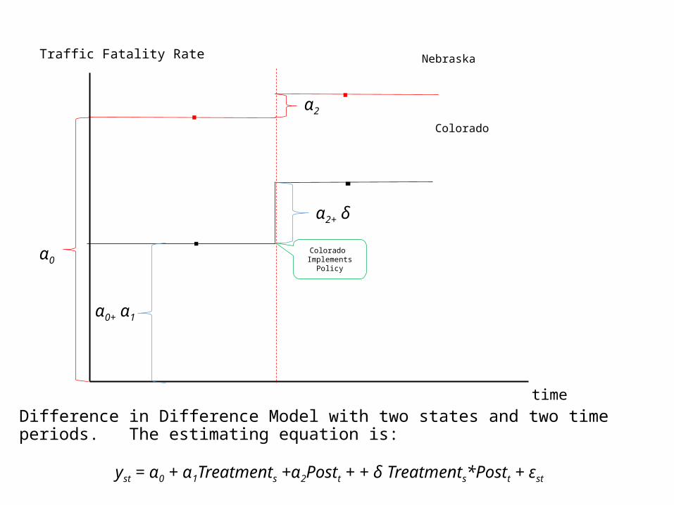
Difference in Difference Model with two states and two time periods. The estimating equation is:

yst = α0 + α1Treatments +α2Postt + + δ Treatments*Postt + εst

Traffic Fatality Rate

time

Colorado

Nebraska

Colorado Implements Policy

α0

α0+ α1

α2

α2+ δ




time

Colorado

Nebraska


α0

α0+ α1

α2

δ

α2




time

Colorado

Nebraska


.

α2

α2

δ

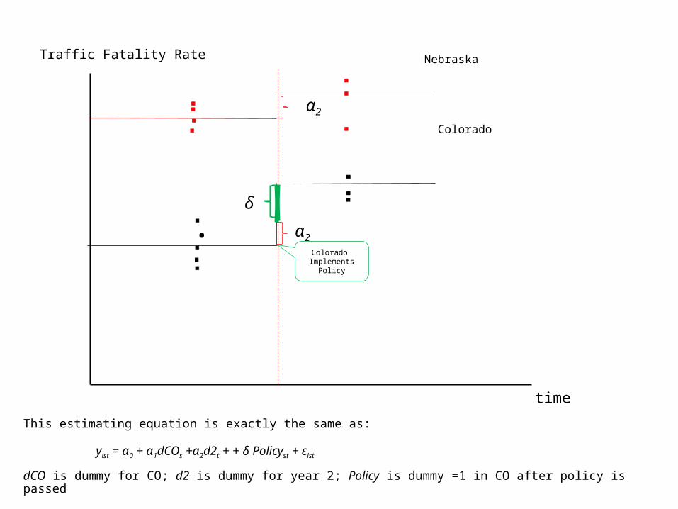
This estimating equation is exactly the same as:

yist = α0 + α1dCOs +α2d2t + + δ Policyst + εist

dCO is dummy for CO; d2 is dummy for year 2; Policy is dummy =1 in CO after policy is passed


time

Colorado

Nebraska


.

α2

α2

δ


time

Colorado

Nebraska

.

The estimate of δ is exactly the same as obtained by subtracting the mean for each state:

α2

δ


time

Colorado

Nebraska

.

And δ is exactly the same after subtracting the mean for each time period:

δ

When we have lots of states and years, an author typically writes

yst = β0 + δPolicyst + vs + zt +εst

And then the author might say that the equation is estimated including state and year fixed effects

Start with state fixed effects, common time trend

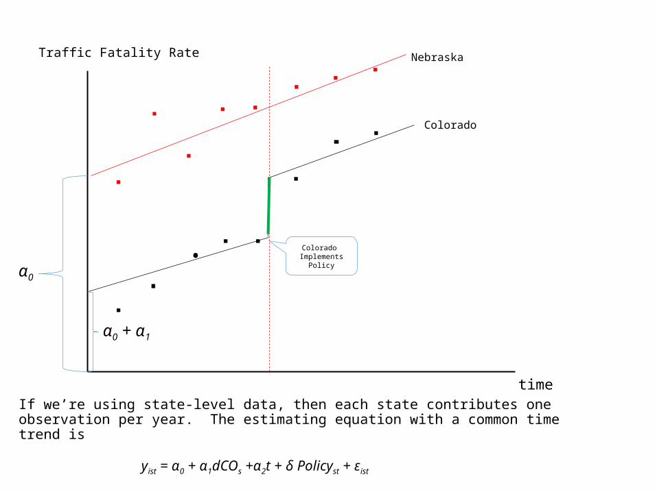
If we’re using state-level data, then each state contributes one observation per year. The estimating equation with a common time trend is

yist = α0 + α1dCOs +α2t + δ Policyst + εist


time

Colorado

Nebraska


.α0

α0 + α1


time

Colorado

Nebraska


.

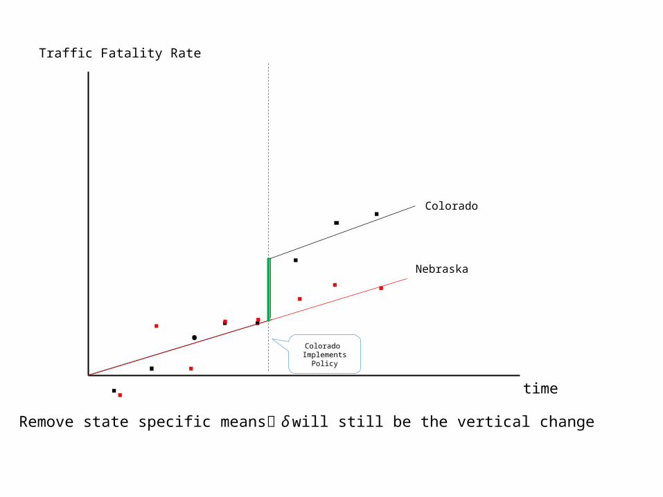
Remove state specific means δ will still be the vertical change


time

Colorado

Nebraska


.New Mexico

New Mexico Implements

Policy

.

With multiple states δ will be the mean vertical change

yst = α0 + α2 t + δPolicyst + vs + εst

If we’re using repeated cross-sectional data at the individual level, then each state contributes multiple observations per year. The estimating equation is:

yist = α0 + δ Policyst + α2 t + vs + εist


time

Colorado

Nebraska


..

.

New Mexico

New Mexico Implements

Policy

.

Now look at time shocks. What if all states experience a common shock in a given year? What if the means varies by time as well as by state?

z3

Crime Rate

time

Barber

Jefferson

Barber legalizes by-the-drink sales

Common time fixed effects-- δ will still be the average vertical change from before and after the policy

Violent Crimect = π0 + δ Wet Lawct + X‘ctπ2 + vc + zt + εct

.Jefferson legalizes by-the-drink sales

Positive shock to crime Negative shock to crime

z3

z8

z8

Crime Rate

time

Barber

Jefferson


But note if you look at it, Barber is increasing faster than Jefferson:

Violent Crimect = π0 + π1Wet Lawct + X‘ctπ2 + vc + zt + εct



Crime Rate

time

Barber

Jefferson


Franklin

Franklin legalizes by-the-drink

sales

Adding state specific time trends Violent Crimect = π0 + δ Wet Lawct + X‘

ctπ2 + vc + zt + Θc∙ t + εct



17

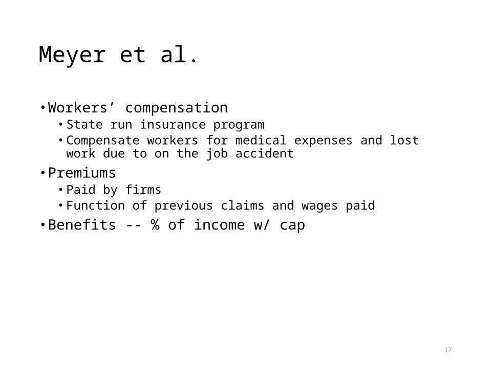
Meyer et al.

• Workers’ compensation• State run insurance program• Compensate workers for medical expenses and lost work due to on the job

accident

• Premiums• Paid by firms• Function of previous claims and wages paid

• Benefits -- % of income w/ cap

18

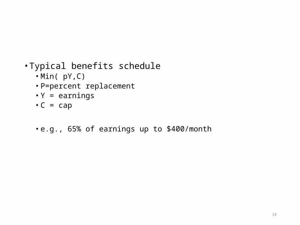
• Typical benefits schedule• Min( pY,C)• P=percent replacement• Y = earnings• C = cap

• e.g., 65% of earnings up to $400/month

19

• Concern: • Moral hazard. Benefits will discourage return to work

• Empirical question: duration/benefits gradient• Previous estimates

• Regress duration (y) on replaced wages (x)• Problem:

• given progressive nature of benefits, replaced wages reveal a lot about the workers

• Replacement rates higher in higher wage states

20

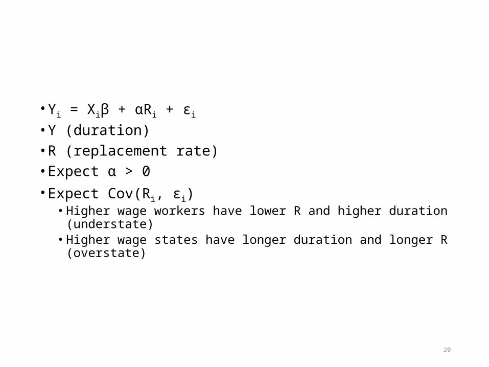
• Yi = Xiβ + αRi + εi

• Y (duration)• R (replacement rate)• Expect α > 0• Expect Cov(Ri, εi)

• Higher wage workers have lower R and higher duration (understate)• Higher wage states have longer duration and longer R (overstate)

21

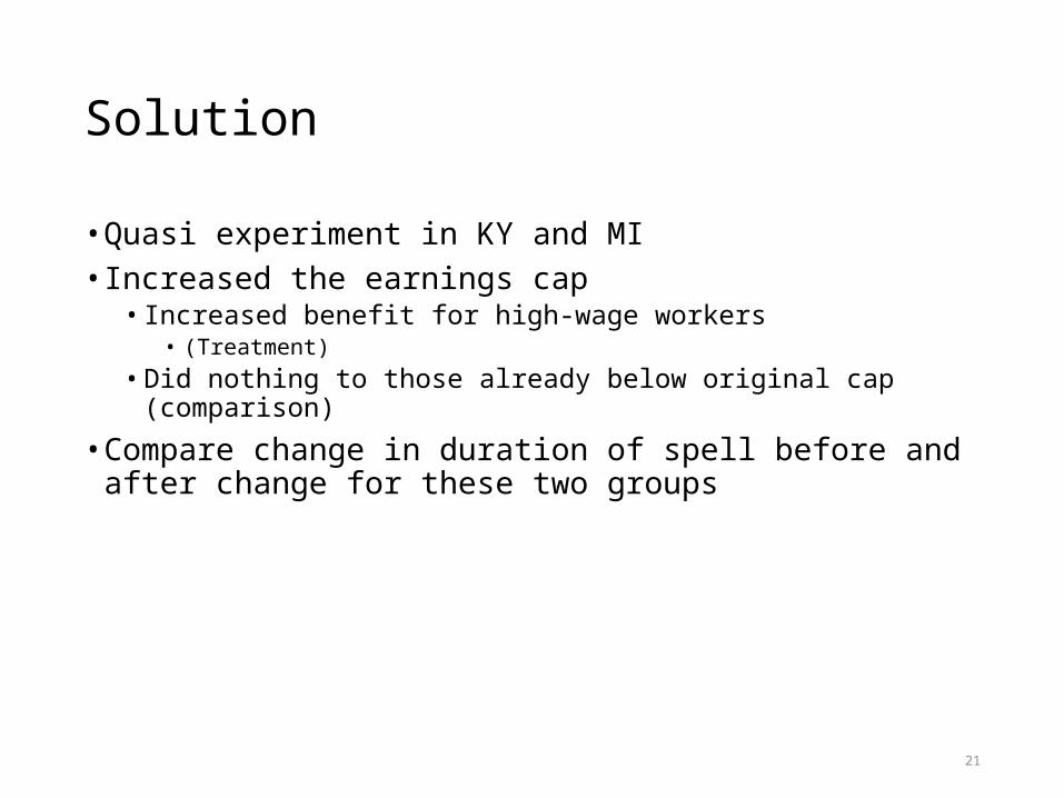
Solution

• Quasi experiment in KY and MI• Increased the earnings cap

• Increased benefit for high-wage workers • (Treatment)

• Did nothing to those already below original cap (comparison)

• Compare change in duration of spell before and after change for these two groups

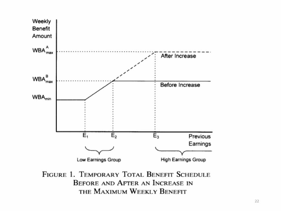
22

23

24

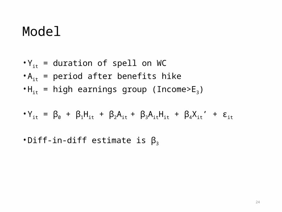
Model

• Yit = duration of spell on WC• Ait = period after benefits hike• Hit = high earnings group (Income>E3)

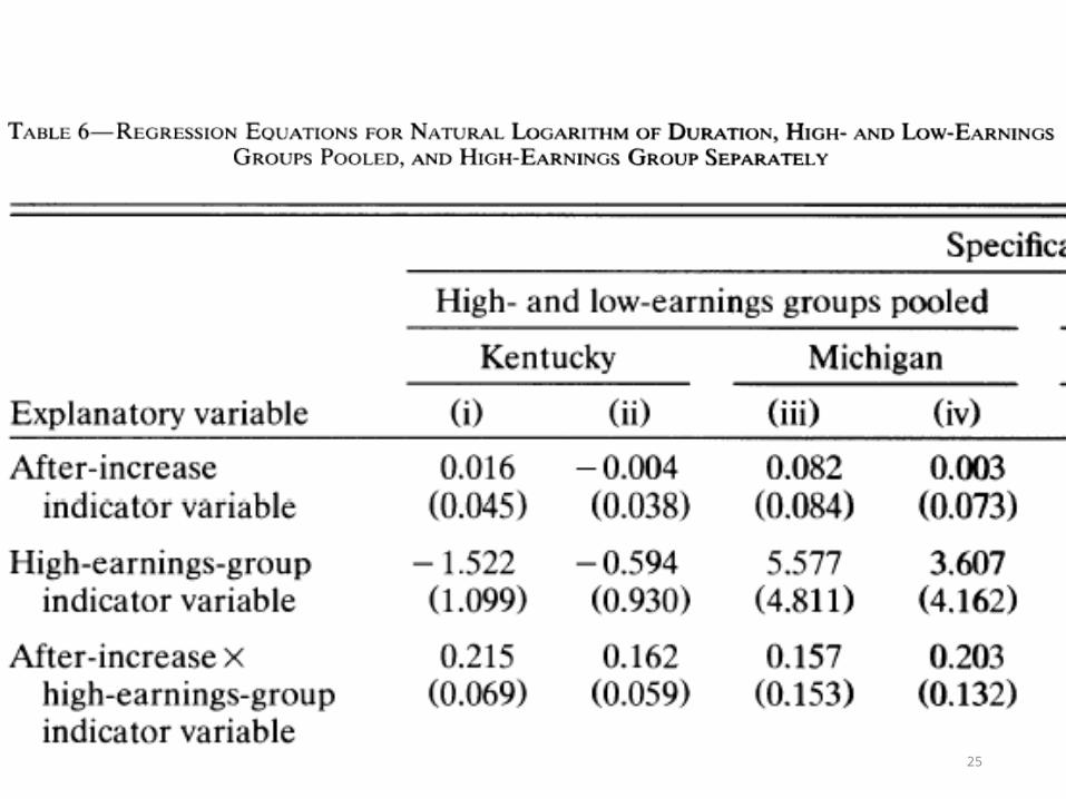
• Yit = β0 + β1Hit + β2Ait + β3AitHit + β4Xit’ + εit

• Diff-in-diff estimate is β3

25

26

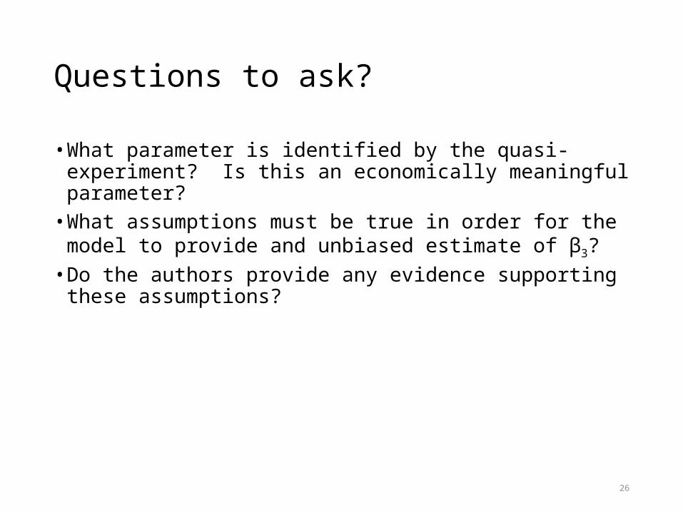
Questions to ask?

• What parameter is identified by the quasi-experiment? Is this an economically meaningful parameter?

• What assumptions must be true in order for the model to provide and unbiased estimate of β3?

• Do the authors provide any evidence supporting these assumptions?

27

Almond et al.

• Neonatal mortality, dies in first 28 days• Infant mortality, died in first year

• Babies born w/ low birth weight(< 2500 grams) are more prone to• Die early in life• Have health problems later in life• Educational difficulties

• generated from cross-sectional regressions• 6% of babies in US are low weight• Highest rate in the developed world

28

• Let Yit be outcome for baby t from mother I• e.g., mortality

• Yit = α + bwit β + Xi γ + αi + εit

• bw is birth weight (grams)• Xi observed characteristics of moms• αi unobserved characteristics of moms

29

• Cross sectional model is of the form

• Yit = α + bwit β + Xi γ + uit

• where uit =αi + εit

• Many observed factors that might explain health (Y) of an infant• Prenatal care, substance abuse, smoking, weight gain (of lack of it)

• Some unobserved as well• Quality of diet, exercise, generic predisposition

• αi not included in model• Cov(bwit,uit) < 0

30

• Solution: Twins• Possess same mother, same environmental characterisitics• Yi1 = α + bwi1 β + Xi γ + αi + εi1

• Yi2 = α + bwi2 β + Xi γ + αi + εi2

• ΔY = Yi2-Yi1 = (bwi2-bwi1) β + (εi2- εi1)

31

Questions to consider?

• What are the conditions under which this will generate unbiased estimate of β?

• What impact (treatment effect) does the model identify?

32

33

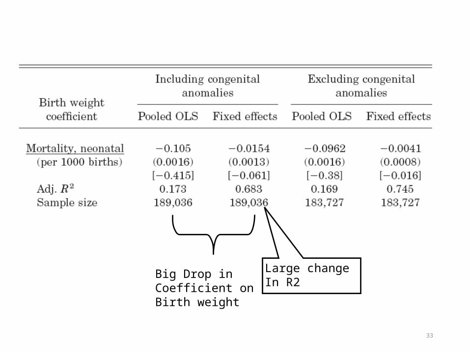
Large changeIn R2

Big Drop in Coefficient onBirth weight

34

35

More general model

• Many within group estimators that do not have the nice discrete treatments outlined above are also called difference in difference models

• Cook and Tauchen. Examine impact of alcohol taxes on heavy drinking

• States tax alcohol• Examine impact on consumption and results of

heavy consumption death due to liver cirrhosis

36

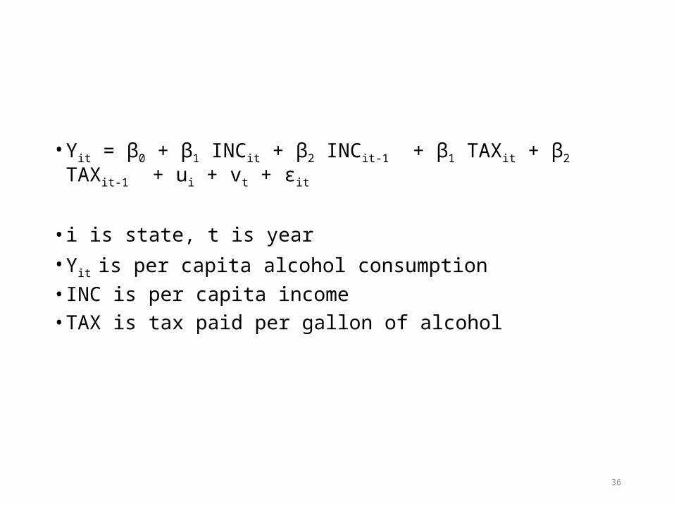
• Yit = β0 + β1 INCit + β2 INCit-1 + β1 TAXit + β2 TAXit-1 + ui + vt + εit

• i is state, t is year• Yit is per capita alcohol consumption• INC is per capita income• TAX is tax paid per gallon of alcohol

37

• Model requires that untreated groups provide estimate of baseline trend would have been in the absence of intervention

• Key – find adequate comparisons• If trends are not aligned, cov(TitAit,εit) ≠0

• Omitted variables bias

• How do you know you have adequate comparison sample?

38

• Concern: suppose that the intervention is more likely in a state with a different trend

• Do the pre-treatment samples look similar?• Tricky. D-in-D model does not require means match – only trends.• If means match, no guarantee trends will• However, if means differ, aren’t you suspicious that trends will as well?

39

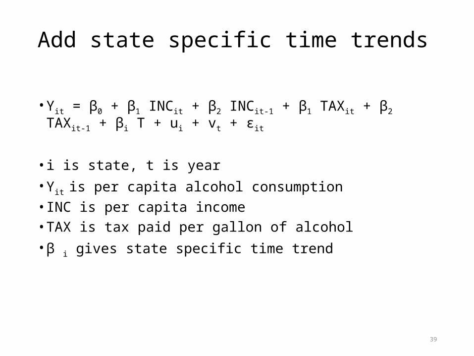
Add state specific time trends

• Yit = β0 + β1 INCit + β2 INCit-1 + β1 TAXit + β2 TAXit-1 + βi T + ui + vt + εit

• i is state, t is year• Yit is per capita alcohol consumption• INC is per capita income• TAX is tax paid per gallon of alcohol• β i gives state specific time trend

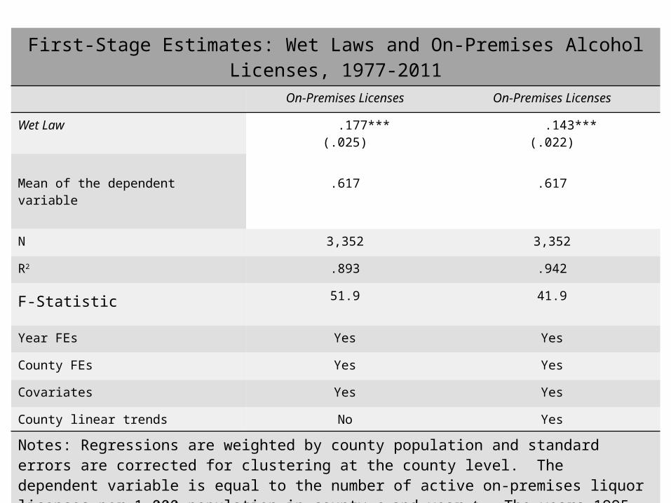
First-Stage Estimates: Wet Laws and On-Premises Alcohol Licenses, 1977-2011On-Premises Licenses On-Premises Licenses

Wet Law .177***(.025)

.143***(.022)

Mean of the dependent variable .617 .617

N 3,352 3,352

R2 .893 .942

F-Statistic 51.9 41.9

Year FEs Yes Yes

County FEs Yes Yes

Covariates Yes Yes

County linear trends No Yes

Notes: Regressions are weighted by county population and standard errors are corrected for clustering at the county level. The dependent variable is equal to the number of active on-premises liquor licenses per 1,000 population in county c and year t. The years 1995, 1996, and 1999 are excluded because of missing crime data.

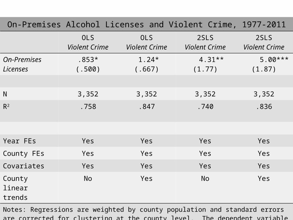
On-Premises Alcohol Licenses and Violent Crime, 1977-2011

OLSViolent Crime

OLSViolent Crime

2SLSViolent Crime

2SLSViolent Crime

On-Premises Licenses

.853*(.500)

1.24*(.667)

4.31**(1.77)

5.00***(1.87)

N 3,352 3,352 3,352 3,352

R2 .758 .847 .740 .836

Year FEs Yes Yes Yes Yes

County FEs Yes Yes Yes Yes

Covariates Yes Yes Yes Yes

County linear trends

No Yes No Yes

Notes: Regressions are weighted by county population and standard errors are corrected for clustering at the county level. The dependent variable is equal to the number of violent crimes per 1,000 population in county c and year t. The years 1995, 1996, and 1999 are excluded because of missing crime data.

42

Falsification tests

• Add “leads” to the model for the treatment• Intervention should not change outcomes before it appears• If it does, then suspicious that covariance between trends and

intervention

• Yit = β0 + β3 Ait + α1Ait-1 + α2 Ait-2 + α3Ait-3 + ui + vt + εit

• Three “leads”• Test null: Ho: α1=α2=α3=0

43

Pick control groups that have similar pre-treatment trends• Most studies pick all untreated data as controls

• Example: Some states raise cigarette taxes. Use states that do not change taxes as controls

• Example: Some states adopt welfare reform prior to TANF. Use all non-reform states as controls

• Can also use econometric procedure to pick controls• Appealing if interventions are discrete and few in number• Easy to identify pre-post

Make slide with no dummies, add time dummy, then state dummy, then interaction term.

Documents

t policy

time dummy

time periods

time shocks

d2 t policy

common time trend slide

policy violent crime

post t treatment s