MAJORIZING FUNCTIONS AND CONVERGENCE OF THE GAUSS-NEWTON METHOD FOR CONVEX COMPOSITE OPTIMIZATION CHONG LI * AND K. F. NG † Abstract. We introduce a notion of quasi-regularity for points with respect to the inclusion F (x) ∈ C where F is a nonlinear Frech´ et differentiable function from R v to R m . When C is the set of minimum points of a convex real-valued function h on R m and F satisfies the L-average Lipschitz condition of Wang, we use the majorizing function technique to establish the semi-local linear/quadratic convergence of sequences generated by the Gauss-Newton method (with quasi-regular initial points) for the convex composite function h ◦ F . Results are new even when the initial point is regular and F is Lipschitz. Key words. The Gauss-Newton method, convex composite optimization, majorizing function, convergence. AMS subject classifications. 47J15 65H10 Secondary, 41A29 1. Introduction . The convex composite optimization to be considered is as follows. min x∈R v f (x) := h(F (x)), (1.1) where h is a real-valued convex function on R m and F is a nonlinear Frech´ et differentiable map from R v to R m (with norm ·). We assume throughout that h attains its minimum h min . This problem has recently received a great deal of attention. As observed by Burke and Ferris in their seminal paper [4], a wide variety of its applications can be found throughout the mathematical programming literature especially in convex inclusion, minimax problems, penalization methods and goal programming, see also [2, 6, 7, 15, 22]; the study of (1.1) not only provides a unifying framework for the development and analysis of algorithmic for solutions but also a convenient tool for the study of first- and second-order optimality conditions in constrained optimization [3, 5, 7, 22]. As in [4, 13], the study of (1.1) naturally relates to the convex inclusion problem F (x) ∈ C, (1.2) where C := argmin h, (1.3) the set of all minimum points of h. Of course it is meaningful to study (1.2) by its own right for a general closed convex set (cf. [14, 16]). In section 3, we introduce a new notion of quasi-regularity for x 0 ∈ R v with respect to the inclusion (1.2). This new notion covers the case of regularity studied by Burke and Ferris [4] as well as the case when F (x 0 ) - C is surjective employed by Robinson [18]. More importantly, we introduce notions of the quasi-regular radius r x0 and of the quasi-regular bound function β x0 attached to * Department of Mathematics, Zhejiang University, Hangzhou 310027, P. R. China, ([email protected]). This author was supported in part by the National Natural Science Foundation of China (grant 10671175) and Program for New Century Excellent Talents in University. † Department of Mathematics, Chinese University of Hong Kong, Hong Kong, P. R. China, ([email protected]). This author was supported by a direct grant (CUHK) and an Earmarked Grant from the Research Grant Council of Hong Kong. 1

Welcome message from author
This document is posted to help you gain knowledge. Please leave a comment to let me know what you think about it! Share it to your friends and learn new things together.
Transcript

MAJORIZING FUNCTIONS AND CONVERGENCE OF THE GAUSS-NEWTONMETHOD FOR CONVEX COMPOSITE OPTIMIZATION
CHONG LI∗ AND K. F. NG†
Abstract. We introduce a notion of quasi-regularity for points with respect to the inclusion F (x) ∈ C where F is a
nonlinear Frechet differentiable function from Rv to Rm. When C is the set of minimum points of a convex real-valued function
h on Rm and F ′ satisfies the L-average Lipschitz condition of Wang, we use the majorizing function technique to establish the
semi-local linear/quadratic convergence of sequences generated by the Gauss-Newton method (with quasi-regular initial points)
for the convex composite function h ◦ F . Results are new even when the initial point is regular and F ′ is Lipschitz.
Key words. The Gauss-Newton method, convex composite optimization, majorizing function, convergence.
AMS subject classifications. 47J15 65H10 Secondary, 41A29
1. Introduction . The convex composite optimization to be considered is as follows.
minx∈Rv
f(x) := h(F (x)), (1.1)
where h is a real-valued convex function on Rm and F is a nonlinear Frechet differentiable map from Rv toRm (with norm ‖ · ‖). We assume throughout that h attains its minimum hmin.
This problem has recently received a great deal of attention. As observed by Burke and Ferris in theirseminal paper [4], a wide variety of its applications can be found throughout the mathematical programmingliterature especially in convex inclusion, minimax problems, penalization methods and goal programming,see also [2, 6, 7, 15, 22]; the study of (1.1) not only provides a unifying framework for the developmentand analysis of algorithmic for solutions but also a convenient tool for the study of first- and second-orderoptimality conditions in constrained optimization [3, 5, 7, 22]. As in [4, 13], the study of (1.1) naturallyrelates to the convex inclusion problem
F (x) ∈ C, (1.2)
where
C := argminh, (1.3)
the set of all minimum points of h. Of course it is meaningful to study (1.2) by its own right for a generalclosed convex set (cf. [14, 16]). In section 3, we introduce a new notion of quasi-regularity for x0 ∈ Rv withrespect to the inclusion (1.2). This new notion covers the case of regularity studied by Burke and Ferris[4] as well as the case when F ′(x0) − C is surjective employed by Robinson [18]. More importantly, weintroduce notions of the quasi-regular radius rx0 and of the quasi-regular bound function βx0 attached to
∗Department of Mathematics, Zhejiang University, Hangzhou 310027, P. R. China, ([email protected]). This author was
supported in part by the National Natural Science Foundation of China (grant 10671175) and Program for New Century
Excellent Talents in University.†Department of Mathematics, Chinese University of Hong Kong, Hong Kong, P. R. China, ([email protected]). This
author was supported by a direct grant (CUHK) and an Earmarked Grant from the Research Grant Council of Hong Kong.
1

2 MAJORIZING FUNCTIONS AND THE GAUSS-NEWTON METHOD
each quasi-regular point x0. For the general case this pair (rx0 , βx0) together with a suitable Lipschiz typeassumption on F ′ enables us to address the issue of convergence of Gauss-Newton sequence provided by thefollowing well known algorithm (cf. [4, 10, 13, 31]).
Algorithm A (η, ∆, x0). Let η ∈ [1,+∞), ∆ ∈ (0,+∞] and for each x ∈ Rv we define D∆(x) by
D∆(x) = {d ∈ Rv : ‖d‖ ≤ ∆, h(F (x) + F ′(x)d) ≤ h(F (x) + F ′(x)d′) ∀d′ ∈ Rv with ‖d′‖ ≤ ∆}. (1.4)
Let x0 ∈ Rv be given. For k = 0, 1, · · · , having x0, x1, · · · , xk, determine xk+1 as follows.
If 0 ∈ D∆(xk) then stop; if 0 /∈ D∆(xk), choose dk such that dk ∈ D∆(xk) and
‖dk‖ ≤ ηd(0, D∆(xk)), (1.5)
and set xk+1 = xk + dk. Here d(x,W ) denotes the distance from x to W in the finite-dimensional Banachspace containing W.
Note that D∆(x) is nonempty and is the solution set of the following convex optimization problem
mind∈Rv,‖d‖≤∆
h(F (x) + F ′(x)d). (1.6)
which can be solved by standard methods such as the subgradient method, the cutting plane method, thebundle method etc (cf. [9]).
If the initial point x0 is a quasi-regular point with (rx0 , βx0) and if F ′ satisfies a Lipschitz type condition(introduced by Wang [28]) with an absolutely continuous function L satisfying a suitable property in relationto (rx0 , βx0), our main results presented in section 4 show that the Gauss-Newton sequence {xn} providedby Algorithm A(η, ∆, x0) converges at a quadratic rate to some x∗ with F (x∗) ∈ C (in particular, x∗ solves(1.1)). Even in the special case when x0 is regular and F ′ is Lipschitz the advantage of allowing βx0 andL to be functions (rather than constants) provides results which are new even for the above special case.Examples are given in section 6 to show there are situations where our results are applicable but not theearlier results in the literature; in particular, Example 6.1 is a simple example to demonstrate a quasi-regular point which is not regular. We shall show that the Gauss-Newton sequence {xn} is “majorized”by the corresponding numerical sequence {tn} generated by the classical Newton method with initial pointt0 = 0 for a “majorizing” function of the following type (again introduced by Wang [28])
φα(t) = ξ − t + α
∫ t
0
L(u)(t− u) du for each t ≥ 0, (1.7)
where ξ, α are positive constants and L is a positive-valued increasing (more precisely, nondecreasing)absolutely continuous function on [0,+∞). In the case when L is a constant function, (1.7) reduces to
φα(t) = ξ − t +αL
2t2 for each t ≥ 0, (1.8)
the majorizing function used by Kantorovich [11, 12]. In the case when
L(u) =2γ
(1− γu)3, (1.9)
(1.7) reduces to
φα(t) = ξ − t +αγt2
1− γt, (1.10)
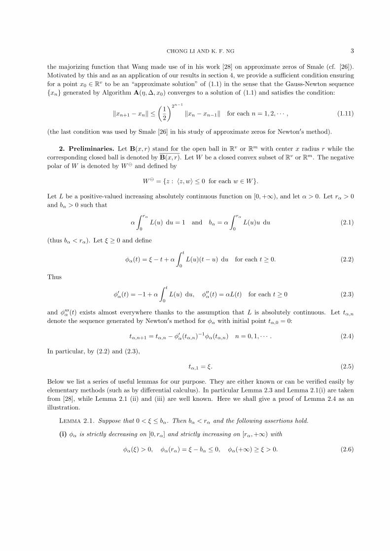
CHONG LI AND K. F. NG 3
the majorizing function that Wang made use of in his work [28] on approximate zeros of Smale (cf. [26]).Motivated by this and as an application of our results in section 4, we provide a sufficient condition ensuringfor a point x0 ∈ Rv to be an “approximate solution” of (1.1) in the sense that the Gauss-Newton sequence{xn} generated by Algorithm A(η, ∆, x0) converges to a solution of (1.1) and satisfies the condition:
‖xn+1 − xn‖ ≤(
12
)2n−1
‖xn − xn−1‖ for each n = 1, 2, · · · , (1.11)
(the last condition was used by Smale [26] in his study of approximate zeros for Newton′s method).
2. Preliminaries. Let B(x, r) stand for the open ball in Rv or Rm with center x radius r while thecorresponding closed ball is denoted by B(x, r). Let W be a closed convex subset of Rv or Rm. The negativepolar of W is denoted by W and defined by
W = {z : 〈z, w〉 ≤ 0 for each w ∈ W}.
Let L be a positive-valued increasing absolutely continuous function on [0,+∞), and let α > 0. Let rα > 0and bα > 0 such that
α
∫ rα
0
L(u) du = 1 and bα = α
∫ rα
0
L(u)u du (2.1)
(thus bα < rα). Let ξ ≥ 0 and define
φα(t) = ξ − t + α
∫ t
0
L(u)(t− u) du for each t ≥ 0. (2.2)
Thus
φ′α(t) = −1 + α
∫ t
0
L(u) du, φ′′α(t) = αL(t) for each t ≥ 0 (2.3)
and φ′′′α (t) exists almost everywhere thanks to the assumption that L is absolutely continuous. Let tα,n
denote the sequence generated by Newton′s method for φα with initial point tα,0 = 0:
tα,n+1 = tα,n − φ′α(tα,n)−1φα(tα,n) n = 0, 1, · · · . (2.4)
In particular, by (2.2) and (2.3),
tα,1 = ξ. (2.5)
Below we list a series of useful lemmas for our purpose. They are either known or can be verified easily byelementary methods (such as by differential calculus). In particular Lemma 2.3 and Lemma 2.1(i) are takenfrom [28], while Lemma 2.1 (ii) and (iii) are well known. Here we shall give a proof of Lemma 2.4 as anillustration.
Lemma 2.1. Suppose that 0 < ξ ≤ bα. Then bα < rα and the following assertions hold.
(i) φα is strictly decreasing on [0, rα] and strictly increasing on [rα,+∞) with
φα(ξ) > 0, φα(rα) = ξ − bα ≤ 0, φα(+∞) ≥ ξ > 0. (2.6)

4 MAJORIZING FUNCTIONS AND THE GAUSS-NEWTON METHOD
Moreover, if ξ < bα, φα has two zeros, denoted respectively by r∗α and r∗∗α , such that
ξ < r∗α <rα
bαξ < rα < r∗∗α , (2.7)
and, if ξ = bα, φα has a unique zero r∗α in (ξ,+∞) (in fact r∗α = rα).
(ii) {tα,n} is strictly monotonically increasing and converges to r∗α.
(iii) The convergence of {tα,n} is of quadratic rate if ξ < bα, and linear if ξ = bα.
Lemma 2.2. Let rα, bα and φα be defined by (2.1) and (2.2). Let α′ > α with the corresponding φα′ .Then the following assertions hold.
(i) The functions α 7→ rα and α 7→ bα are strictly decreasing on (0,+∞).
(ii) φα < φα′ on (0,+∞).
(iii) The function α 7→ r∗α is strictly increasing on the interval I(ξ), where I(ξ) denotes the set of allα > 0 such that ξ ≤ bα.
Lemma 2.3. Let 0 ≤ c < +∞. Define
χ(t) =1t2
∫ t
0
L(c + u)(t− u) du, 0 ≤ t < +∞. (2.8)
Then χ is increasing on [0,+∞).
Lemma 2.4. Define
ωα(t) = φ′α(t)−1φα(t) t ∈ [0, r∗α).
Suppose that 0 < ξ ≤ bα. Then ωα is increasing on [0, r∗α).
Proof. Since
ω′α(t) =φ′α(t)2 − φα(t)φ′′α(t)
φ′α(t)2for each t ∈ [0, r∗α),
it suffices to show that
ζα(t) := φ′α(t)2 − φα(t)φ′′α(t) ≥ 0 for each t ∈ [0, r∗α).
Since ζα(r∗α) = φ′α(r∗α)2 ≥ 0, it remains to show that ζα is decreasing on [0, r∗α]. To do this, note that by(2.3) ζα is absolutely continuous and so the derivative of ζα exists almost everywhere on [0, r∗α] with
ζ ′α(t) = φ′α(t)φ′′α(t)− φα(t)φ′′′α (t) ≤ 0 a.e t ∈ [0, r∗α).
because φ′α ≤ 0 while φα, φ′′α, φ′′′α ≥ 0 a.e. on [0, r∗α). Therefore, ζα is decreasing on [0, r∗α) and the proof iscomplete. �
The following conditions were introduced by Wang in [28] but using the terminologies of “the centerLipschitz condition with the L average” and “the center Lipschitz condition in the inscribed sphere with theL average” respectively for (a) and (b).

CHONG LI AND K. F. NG 5
Definition 2.5. Let Y be a Banach space and let x0 ∈ Rv. Let G be a mapping from Rv to Y . ThenG is said to satisfy
(a) the weak L-average Lipschitz condition on B(x0, r) if
‖G(x)−G(x0)‖ ≤∫ ‖x−x0‖
0
L(u) du for each x ∈ B(x0, r); (2.9)
(b) the L-average Lipschitz condition on B(x0, r), if
‖G(x)−G(x′)‖ ≤∫ ‖x−x′‖+‖x′−x0‖
‖x′−x0‖L(u) du for all x, x′ ∈ B(x0, r) with ‖x− x′‖+ ‖x′ − x0‖ ≤ r.(2.10)
3. Regularities. Let C be a closed convex set in Rm. Consider the inclusion
F (x) ∈ C. (3.1)
Let x ∈ Rv and
D(x) = {d ∈ Rv : F (x) + F ′(x)d ∈ C}. (3.2)
Remark 3.1. In the case when C is the set of all minimum points of h and if there exists d0 ∈ Rv with‖d0‖ ≤ ∆ such that d0 ∈ D(x), then d0 ∈ D∆(x) and for each d ∈ Rv with ‖d‖ ≤ ∆ one has
d ∈ D∆(x) ⇐⇒ d ∈ D(x) ⇐⇒ d ∈ D∞(x). (3.3)
Remark 3.2. The set D(x) defined in (3.2) can be viewed as the solution set of the following “linearized”problem associated with (3.1):
(Px) : F (x) + F ′(x) d ∈ C. (3.4)
Thus β(‖x− x0‖) in (3.5) is an ”error bound” in determining how far the origin is away from the solutionset of (Px).
Definition 3.1. A point x0 ∈ Rv is called a quasi-regular point of the inclusion (3.1) if there existr ∈ (0,+∞) and an increasing positive-valued function β on [0, r) such that
D(x) 6= ∅ and d(0,D(x)) ≤ β(‖x− x0‖) d(F (x), C) for all x ∈ B(x0, r). (3.5)
Let rx0 denote the supremum of r such that (3.5) holds for some increasing positive-valued function β
on [0, r). Let r ∈ [0, rx0 ] and let Br(x0) denote the set of all increasing positive-valued function β on [0, r)such that (3.5) holds. Define
βx0(t) = inf{β(t) : β ∈ Brx0(x0)} for each t ∈ [0, rx0). (3.6)

6 MAJORIZING FUNCTIONS AND THE GAUSS-NEWTON METHOD
Note that each β ∈ Br(x0) with limt→r− β(t) < +∞ can be extended to an element of Brx0(x0). From this
we can verify that
βx0(t) = inf{β(t) : β ∈ Br(x0)} for each t ∈ [0, r). (3.7)
We call rx0 and βx0 respectively the quasi-regular radius and the quasi-regular bound function of the quasi-regular point x0.
Definition 3.2. A point x0 ∈ Rv is a regular point of the inclusion (3.1) if
ker(F ′(x0)T ) ∩ (C − F (x0)) = {0}. (3.8)
The notion of regularity relates to some other notions of regularity that can be found in the papers [1, 3,20, 21, 25], which have played an important role in the study of nonsmooth optimizations. Some equivalentconditions on the regular points for (3.1) are given in [4]. In the following proposition the existence ofconstants r and β is due to Burke-Ferris [4] and the second assertion then follows from a remark afterDefinition 3.1
Proposition 3.3. Let x0 be a regular point of (3.1). Then there are constants r > 0 and β > 0 suchthat (3.5) holds for r and β(·) = β; consequently, x0 is a quasi-regular point with the quasi-regular radiusrx0 ≥ r and the quasi-regular bound function βx0 ≤ β on [0, r].
Another important link of the present study relates to Robinson’s condition [18, 19] that the convexprocess d 7→ F ′(x)d− C is onto Rm. To see this, let us first recall the concept of convex process which wasintroduced by Rockafeller [23, 24] for convexity problems (see also Robinson [19]).
Definition 3.4. A set-valued mapping T : Rv → 2Rm
is called a convex process from Rv to Rm if itsatisfies
(a) T (x + y) ⊇ Tx + Ty for all x, y ∈ Rv;
(b) Tλx = λTx for all λ > 0, x ∈ Rv;
(c) 0 ∈ T0.
Thus T : Rv → 2Rm
is a convex process if and only if its graph Gr(T ) is a convex cone in Rv × Rm. Asusual, the domain, range and inverse of a convex process T are respectively denoted by D(T ), R(T ), T−1;i.e.,
D(T ) = {x ∈ Rv : Tx 6= ∅},
R(T ) = ∪{Tx : x ∈ D(T )},
T−1y = {x ∈ Rv : y ∈ Tx}.
Obviously T−1 is a convex process from Rm to Rv. Furthermore, for a set A in a Rv or Rv, it would beconvenient to use the notation ‖A‖ to denote its distance to the origin, that is,
‖A‖ = inf{‖a‖ : a ∈ A}. (3.9)

CHONG LI AND K. F. NG 7
Definition 3.5. Suppose that T is a convex process. The norm of T is defined by
‖T‖ = sup{‖Tx‖ : x ∈ D(T ), ‖x‖ ≤ 1}.
If ‖T‖ < +∞, we say the convex process T is normed.
For two convex processes T and S from Rv to Rm, the addition and multiplication are defined respectivelyas follows.
(T + S)(x) = Tx + Sx for each x ∈ Rv,
(λT )(x) = λ(Tx) for each x ∈ Rv and λ ∈ R.
Let C be a closed convex set in Rm and let x ∈ Rv. We define Tx by
Txd = F ′(x) d− C for each d ∈ Rv. (3.10)
Then its inverse is
T−1x y = {d ∈ Rv : F ′(x) d ∈ y + C} for each y ∈ Rm. (3.11)
Note that Tx is a convex process in the case when C is a cone. Note also that D(Tx) = Rv for each x ∈ Rv
and D(T−1x0
) = Rm if x0 ∈ Rv is such that the following condition of Robinson is satisfied:
Tx0 carries Rv onto Rm. (3.12)
Proposition 3.7 below shows that condition of Robinson (3.12) implies that x0 is a regular point of (3.1)and an estimate of the quasi-regular bound function is provided. For its proof we need the following lemmawhich is known in [18].
Lemma 3.6. Let C be a closed convex cone in Rm and let x0 ∈ Rv be such that the condition of Robinson(3.12) is satisfied. Then the following assertions hold:
(i) T−1x0
is normed.
(ii) If S is a linear transformation from Rv to Rm such that ‖T−1x0‖‖S‖ < 1, then the convex process T
defined by
T = Tx0 + S
carries Rv onto Rm. Furthermore, T−1 is normed and
‖T−1‖ ≤‖T−1
x0‖
1− ‖T−1x0 ‖‖S‖
.
Proposition 3.7. Let x0 ∈ Rv and let Tx0 be defined as in (3.10). Suppose that the condition ofRobinson (3.12) is satisfied. Then the following assertion hold.
(i) x0 is a regular point of (3.1).

8 MAJORIZING FUNCTIONS AND THE GAUSS-NEWTON METHOD
(ii) Suppose further that C is a closed convex cone in Rm and F ′ satisfies the weak L-average Lipschitzcondition on B(x0, r) for some r > 0. Let β0 = ‖T−1
x0‖ and let rβ0 be defined by
β0
∫ rβ0
0
L(u) du = 1 (3.13)
(cf. (2.1)). Then the quasi-regular radius rx0 and the quasi-regular bound function βx0 satisfy rx0 ≥min{r, rβ0} and
βx0(t) ≤β0
1− β0
∫ t
0
L(u) du
for each t with 0 ≤ t < min{r, rβ0}. (3.14)
Proof. Suppose that the condition (3.12) is satisfied and let y belong to the set of the intersection in (3.8).Then, in view of the definition of Tx0 , there exist u ∈ Rv and c ∈ C such that −y − F (x0) = F ′(x0)u − c.Hence
〈y, F ′(x0)u〉 = 〈F ′(x0)T y, u〉 = 0 and 〈y, c− F (x0)〉 ≤ 0. (3.15)
It follows that
〈y, y〉 = 〈y, c− F (x0)− F ′(x0)u〉 = 〈y, c− F (x0)〉 ≤ 0 (3.16)
and hence y = 0. This shows that (3.8) holds and so x0 is a regular point of the inclusion (3.1).
Now let r > 0 and suppose that F ′ satisfies the weak L-average Lipschitz condition on B(x0, r). Letx ∈ Rv such that ‖x− x0‖ < min{r, rβ0}. Then
‖F ′(x)− F ′(x0)‖ ≤∫ ‖x−x0‖
0
L(u) du <
∫ rβ0
0
L(u) du;
hence, by (3.13),
‖T−1x0‖‖F ′(x)− F ′(x0)‖ < ‖T−1
x0‖∫ rβ0
0
L(u) du = 1.
This with Lemma 3.6 implies that the convex process defined by
Txd = F ′(x) d− C = Tx0d + [F ′(x)− F ′(x0)] d for each d ∈ Rv
carries Rv onto Rm and
‖T−1x ‖ ≤
‖T−1x0‖
1− ‖T−1x0 ‖‖F ′(x)− F ′(x0)‖
≤‖T−1
x0‖
1− ‖T−1x0 ‖
∫ ‖x−x0‖
0
L(u) du
. (3.17)
Since Tx is surjective, we have that D(x) is nonempty; in particular, for each c ∈ C,
T−1x (c− F (x)) ⊆ D(x) (3.18)
To see this, let d ∈ T−1x (c − F (x)). Then, by (3.11), one has that F ′(x) d ∈ c − F (x) + C ⊆ C − F (x) and
so F (x) + F ′(x) d ∈ C, that is, d ∈ D(x). Hence (3.18) is true. Consequently,
d(0,D(x)) ≤ ‖T−1x (c− F (x))‖ ≤ ‖T−1
x ‖‖c− F (x)‖.
CHONG LI AND K. F. NG 9
Since this is valid for each c ∈ C, it is seen that
d(0,D(x)) ≤ ‖T−1x ‖d(F (x), C).
Combining this with (3.17) and (3.6) gives the desired result (3.14), and the proof is complete. �
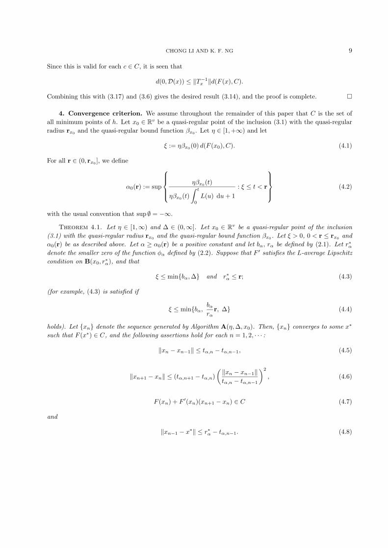
4. Convergence criterion. We assume throughout the remainder of this paper that C is the set ofall minimum points of h. Let x0 ∈ Rv be a quasi-regular point of the inclusion (3.1) with the quasi-regularradius rx0 and the quasi-regular bound function βx0 . Let η ∈ [1,+∞) and let
ξ := ηβx0(0) d(F (x0), C). (4.1)
For all r ∈ (0, rx0 ], we define
α0(r) := sup
ηβx0(t)
ηβx0(t)∫ t
0
L(u) du + 1: ξ ≤ t < r
(4.2)
with the usual convention that sup ∅ = −∞.
Theorem 4.1. Let η ∈ [1,∞) and ∆ ∈ (0,∞]. Let x0 ∈ Rv be a quasi-regular point of the inclusion(3.1) with the quasi-regular radius rx0 and the quasi-regular bound function βx0 . Let ξ > 0, 0 < r ≤ rx0 andα0(r) be as described above. Let α ≥ α0(r) be a positive constant and let bα, rα be defined by (2.1). Let r∗αdenote the smaller zero of the function φα defined by (2.2). Suppose that F ′ satisfies the L-average Lipschitzcondition on B(x0, r
∗α), and that
ξ ≤ min{bα,∆} and r∗α ≤ r; (4.3)
(for example, (4.3) is satisfied if
ξ ≤ min{bα,bα
rαr, ∆} (4.4)
holds). Let {xn} denote the sequence generated by Algorithm A(η, ∆, x0). Then, {xn} converges to some x∗
such that F (x∗) ∈ C, and the following assertions hold for each n = 1, 2, · · · :
‖xn − xn−1‖ ≤ tα,n − tα,n−1, (4.5)
‖xn+1 − xn‖ ≤ (tα,n+1 − tα,n)(‖xn − xn−1‖tα,n − tα,n−1
)2
, (4.6)
F (xn) + F ′(xn)(xn+1 − xn) ∈ C (4.7)
and
‖xn−1 − x∗‖ ≤ r∗α − tα,n−1. (4.8)
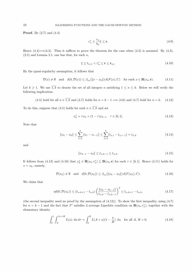
10 MAJORIZING FUNCTIONS AND THE GAUSS-NEWTON METHOD
Proof. By (2.7) and (4.4)
r∗α ≤rα
bαξ ≤ r. (4.9)
Hence (4.4)=⇒(4.3). Thus it suffices to prove the theorem for the case when (4.3) is assumed. By (4.3),(2.5) and Lemma 2.1, one has that, for each n,
ξ ≤ tα,n < r∗α ≤ r ≤ rx0 . (4.10)
By the quasi-regularity assumption, it follows that
D(x) 6= ∅ and d(0,D(x)) ≤ βx0(‖x− x0‖) d(F (x), C) for each x ∈ B(x0, r). (4.11)
Let k ≥ 1. We use 1, k to denote the set of all integers n satisfying 1 ≤ n ≤ k. Below we will verify thefollowing implication:
(4.5) hold for all n ∈ 1, k and (4.7) holds for n = k − 1 =⇒ (4.6) and (4.7) hold for n = k. (4.12)
To do this, suppose that (4.5) holds for each n ∈ 1, k and set
xτk = τxk + (1− τ)xk−1 τ ∈ [0, 1]. (4.13)
Note that
‖xk − x0‖ ≤k∑
i=1
‖xi − xi−1‖ ≤k∑
i=1
(tα,i − tα,i−1) = tα,k (4.14)
and
‖xk−1 − x0‖ ≤ tα,k−1 ≤ tα,k. (4.15)
It follows from (4.13) and (4.10) that xτk ∈ B(x0, r
∗α) ⊆ B(x0, r) for each τ ∈ [0, 1]. Hence (4.11) holds for
x = xk, namely,
D(xk) 6= ∅ and d(0,D(xk)) ≤ βx0(‖xk − x0‖) d(F (xk), C). (4.16)
We claim that
ηd(0,D(xk)) ≤ (tα,k+1 − tα,k)(‖xk − xk−1‖tα,k − tα,k−1
)2
≤ tα,k+1 − tα,k, (4.17)
(the second inequality need no proof by the assumption of (4.12)). To show the first inequality, using (4.7)for n = k − 1 and the fact that F ′ satisfies L-average Lipschitz condition on B(x0, r
∗α), together with the
elementary identity∫ 1
0
∫ A+τB
A
L(u) du dτ =∫ B
0
L(A + u)(1− u
B) du for all A, B > 0, (4.18)

CHONG LI AND K. F. NG 11
we have by (4.16) that
ηd(0,D(xk)) ≤ ηβx0(‖xk − x0‖)d(F (xk), C)≤ ηβx0(‖xk − x0‖)‖F (xk)− F (xk−1)− F ′(xk−1)(xk − xk−1)‖
≤ ηβx0(‖xk − x0‖)∥∥∥∥∫ 1
0
(F ′(xτk)− F ′(xk−1))(xk − xk−1) dτ
∥∥∥∥≤ ηβx0(‖xk − x0‖)
∫ 1
0
(∫ τ‖xk−xk−1‖+‖xk−1−x0‖
‖xk−1−x0‖L(u) du
)‖xk − xk−1‖ dτ
= ηβx0(‖xk − x0‖)
(∫ ‖xk−xk−1‖
0
L(‖xk−1 − x0‖+ u)(‖xk − xk−1‖ − u) du
)
≤ ηβx0(tα,k)
(∫ ‖xk−xk−1‖
0
L(tα,k−1 + u)(‖xk − xk−1‖ − u) du
),
where the last inequality is valid because L and βx0 are increasing and thanks to (4.14) and (4.15). Since(4.5) holds for n = k, Lemma 2.3 implies that∫ ‖xk−xk−1‖
0
L(tα,k−1 + u)(‖xk − xk−1‖ − u) du
‖xk − xk−1‖2≤
∫ tα,k−tα,k−1
0
L(tα,k−1 + u)(tα,k − tα,k−1 − u) du
(tα,k − tα,k−1)2
and it follows from the earlier estimate that
ηd(0,D(xk)) ≤ ηβx0(tα,k)(∫ tα,k−tα,k−1
0
L(tα,k−1 + u)(tα,k − tα,k−1 − u)du
)(‖xk − xk−1‖tα,k − tα,k−1
)2
. (4.19)
Similarly by (2.2), (2.3), (2.4) and (4.18), we have
φα(tα,k) = φα(tα,k)− φα(tα,k−1)− φ′α(tα,k−1)(tα,k − tα,k−1)
=(∫ 1
0
[φ′α(tα,k−1 + τ(tα,k − tα,k−1))− φ′α(tα,k−1)] d τ
)(tα,k − tα,k−1)
=
(α
∫ 1
0
∫ τ(tα,k−tα,k−1)+tα,k−1
tα,k−1
L(u) du dτ
)(tα,k − tα,k−1)
= α
∫ tα,k−tα,k−1
0
L(tα,k−1 + u)(tα,k − tα,k−1 − u) du. (4.20)
On the other hand, by (4.10) and (4.2),
ηβx0(tα,k)α0(r)
≤(
1− α0(r)∫ tα,k
0
L(u) du
)−1
.
Since α ≥ α0(r) and by (2.3), it follows that
ηβx0(tα,k)α
≤(
1− α
∫ tα,k
0
L(u) du
)−1
= −(φ′α(tα,k))−1. (4.21)
Combining (4.19)-(4.21) together with (2.4), the first inequality in (4.17) is seen to hold. Moreover by Lemma2.4 and (4.3), we have
tα,k+1 − tα,k = −φ′α(tα,k)−1φα(tα,k) ≤ −φ′α(tα,0)−1φα(tα,0) = ξ ≤ ∆,

12 MAJORIZING FUNCTIONS AND THE GAUSS-NEWTON METHOD
so (4.17) implies that d(0,D(xk)) ≤ ∆. Hence there exists d0 ∈ Rv with ‖d0‖ ≤ ∆ such that F (xk) +F ′(xk)d0 ∈ C. Consequently, by Remark 3.1,
D∆(xk) = {d ∈ Rv : ‖d‖ ≤ ∆, F (xk) + F ′(xk)d ∈ C}
and
d(0, D∆(xk)) = d(0,D(xk)).
Since dk = xk+1−xk ∈ D∆(xk) by Algorithm A(η, ∆, x0), it follows that (4.7) holds for n = k. Furthermore,one has that
‖xk+1 − xk‖ ≤ ηd(0, D∆(xk)) = ηd(0,D(xk)).
This with (4.17) yields that (4.6) holds for n = k and hence implication (4.12) is proved.
Clearly, if (4.5) holds for each n = 1, 2, · · · , then {xn} is a Cauchy sequence by the monotonicity of {tn}and hence converges to some x∗. Thus (4.8) is clear. Therefore, to prove the theorem, we only need to provethat (4.5), (4.6) and (4.7) hold for each n = 1, 2, · · · . We will proceed by the mathematical induction. First,by (4.1), (4.3) and (4.11), D(x0) 6= ∅ and
ηd(0,D(x0)) ≤ ηβx0(‖x0 − x0‖) d(F (x0), C) = ηβx0(0)d(F (x0), C) = ξ ≤ ∆.
Then using the same arguments just used above, we have that (4.7) holds for n = 0 and
‖x1 − x0‖ = ‖d0‖ ≤ ηd(0, D∆(x0)) ≤ ηβx0(0)d(F (x0), C) = ξ = tα,1 − tα,0;
that is, (4.5) holds for n = 1. Thus, by (4.12), (4.6) and (4.7) hold for n = 1. Furthermore, assume that(4.5), (4.6) and (4.7) hold for all 1 ≤ n ≤ k. Then
‖xk+1 − xk‖ ≤ (tα,k+1 − tα,k)(‖xk − xk−1‖tα,k − tα,k−1
)2
≤ tα,k+1 − tα,k.
This shows that (4.5) holds for n = k + 1 and hence (4.5) holds for all n with 1 ≤ n ≤ k + 1. Thus, (4.12)implies that (4.6) and (4.7) hold for n = k + 1. Therefore, (4.5), (4.6) and (4.7) hold for each n = 1, 2, · · · .The proof is complete. �
Remark 4.1. (a) In Theorem 4.1 if one assumes in addition that either (i) ξ < bα or (ii) α > α0 :=α0(r), then the convergence of the sequence {xn} is of quadratic rate. For the case of (i), this remark followsfrom immediately from Lemma 2.1 (iii) thanks to (4.5) and (4.8). If (ii) is assumed then, by Lemma 2.2,ξ ≤ bα < bα0 and r∗α0
≤ r∗α ≤ r. Hence (4.3) holds with α0 in place of α. Since ξ < bα0 , we are now in thecase (i) if α is replaced by α0 and hence our remark here is established.
(b) Refinements for results presented in the remainder of this paper can also be established in the similarmanner as in (a) above.
Remark 4.2. Suppose that there exits a pair (α, r) such that{α = α0(r)r∗α = r.
(4.22)

CHONG LI AND K. F. NG 13
Note that the functions α 7→ bα is decreasing by Lemma 2.2. Then, if (4.3) holds for some (α, r) with α ≥ α
and r ≥ r, (4.3) does for (α, r) = (α, r) (hence Theorem 4.1 is applicable).
Recall from Proposition 3.3 that the assumption for the existence of r, β in the following corollary isautomatically satisfied when x0 ∈ Rv is a regular point of the inclusion (3.1). This remark also applies toTheorems 5.1, 5.6 and Corollary 5.2.
Corollary 4.2. Let x0 ∈ Rv be a regular point of the inclusion (3.1) with r > 0 and β > 0 such that
D(x) 6= ∅ and d(0,D(x)) ≤ β d(F (x), C) for all x ∈ B(x0, r). (4.23)
Let η ∈ [1,∞), ∆ ∈ (0,∞], ξ = ηβd(F (x0), C),
α =ηβ
1 + ηβ∫ ξ
0L(u)du
(4.24)
and let bα, rα be defined by (2.1). Let r∗α denote the smaller zero of the function φα defined by (2.2). Supposethat F ′ satisfies the L-average Lipschitz condition on B(x0, r
∗α) and that
ξ ≤ min{bα,∆} and r∗α ≤ r; (4.25)
(for example, (4.25) is satisfied if
ξ ≤ min{bα,bα
rαr, ∆} (4.26)
holds). Then the conclusions of Theorem 4.1 hold.
Proof. Note that ξ < rα∗ ≤ r by Lemma 2.1 and (4.25). By (3.6) and (3.7), it is clear that rx0 ≥ r and
βx0(·) ≤ β on [0, r). Let r := r and let α0(r) be defined by (4.2) as in Theorem 4.1. Then, by (4.24), wehave that
α ≥ ηβx0(t)
1 + ηβx0(t)∫ t
0
L(u) du
for each t ∈ [ξ, r).
Hence α ≥ α0(r) by (4.2). Note that (4.26) (resp. (4.25)) is identical to (4.4) (resp. (4.3)), Theorem 4.1 isapplicable and the proof is complete. �
Corollary 4.3. Let η ∈ [1,+∞), ∆ ∈ (0,+∞] and let C be a cone. Let x0 ∈ Rv be such that Tx0
carries Rv onto Rm. Let
ξ = η‖T−1x0‖ d(F (x0), C), (4.27)
α =η‖T−1
x0‖
1 + (η − 1)‖T−1x0 ‖
∫ ξ
0
L(u) du
(4.28)
and let bα, rα be defined by (2.1). Let r∗α denote the smaller zero of the function φα defined by (2.2). Supposethat F ′ satisfies the L-average Lipschitz condition on B(x0, r
∗α) and that
ξ ≤ min{bα,∆}. (4.29)
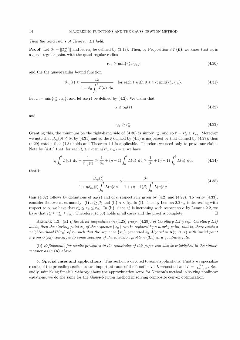
14 MAJORIZING FUNCTIONS AND THE GAUSS-NEWTON METHOD
Then the conclusions of Theorem 4.1 hold.
Proof. Let β0 = ‖T−1x0‖ and let rβ0 be defined by (3.13). Then, by Proposition 3.7 (ii), we know that x0 is
a quasi-regular point with the quasi-regular radius
rx0 ≥ min{r∗α, rβ0} (4.30)
and the the quasi-regular bound function
βx0(t) ≤β0
1− β0
∫ t
0
L(u) du
for each t with 0 ≤ t < min{r∗α, rβ0}. (4.31)
Let r := min{r∗α, rβ0}, and let α0(r) be defined by (4.2). We claim that
α ≥ α0(r) (4.32)
and
rβ0 ≥ r∗α. (4.33)
Granting this, the minimum on the right-hand side of (4.30) is simply r∗α, and so r = r∗α ≤ rx0 . Moreoverwe note that βx0(0) ≤ β0 by (4.31) and so the ξ defined by (4.1) is majorized by that defined by (4.27); thus(4.29) entails that (4.3) holds and Theorem 4.1 is applicable. Therefore we need only to prove our claim.Note by (4.31) that, for each ξ ≤ t < min{r∗α, rβ0} = r, we have
η
∫ t
0
L(u) du +1
βx0(t)≥ 1
β0+ (η − 1)
∫ t
0
L(u) du ≥ 1β0
+ (η − 1)∫ ξ
0
L(u) du, (4.34)
that is,
βx0(t)
1 + ηβx0(t)∫ t
0
L(u)du
≤ β0
1 + (η − 1)β0
∫ t
0
L(u)du
; (4.35)
thus (4.32) follows by definitions of α0(r) and of α respectively given by (4.2) and (4.28). To verify (4.33),consider the two cases namely: (i) α ≥ β0 and (ii) α < β0. In (i), since by Lemma 2.2 rα is decreasing withrespect to α, we have that r∗α ≤ rα ≤ rβ0 . In (ii), since r∗α is increasing with respect to α by Lemma 2.2, wehave that r∗α ≤ r∗β0
≤ rβ0 . Therefore, (4.33) holds in all cases and the proof is complete. �
Remark 4.3. (a) If the strict inequalities in (4.25) (resp. (4.29)) of Corollary 4.2 (resp. Corollary 4.3)holds, then the starting point x0 of the sequence {xn} can be replaced by a nearby point, that is, there exists aneighbourhood U(x0) of x0 such that the sequence {xn} generated by Algorithm A(η, ∆, x) with initial pointx from U(x0) converges to some solution of the inclusion problem (3.1) at a quadratic rate.
(b) Refinements for results presented in the remainder of this paper can also be established in the similarmanner as in (a) above.
5. Special cases and applications. This section is devoted to some applications. Firstly we specializeresults of the preceding section to two important cases of the function L: L =constant and L = 2γ
(1−γu)3 . Sec-ondly, mimicking Smale′s γ-theory about the approximation zeros for Newton′s method in solving nonlinearequations, we do the same for the Gauss-Newton method in solving composite convex optimization.

CHONG LI AND K. F. NG 15
5.1. Kantorovich type. Throughout this subsection, we assume that the function L is a constantfunction. Then, by (2.1) and (2.2), we have that, for all α > 0,
rα =1
αL, bα =
12αL
(5.1)
and
φα(t) = ξ − t +αL
2t2.
Moreover, if ξ ≤ 12αL , then the zeros of φα are given by
r∗αr∗∗α
}=
1∓√
1− 2αLξ
αL. (5.2)
It is also known (see for example [8, 17, 29]) that {tα,n} has the closed form
tα,n =1− q2n−1
α
1− q2n
α
r∗α for each n = 0, 1, · · · , (5.3)
where
qα :=r∗αr∗∗α
=1−
√1− 2αLξ
1 +√
1− 2αLξ. (5.4)
For the present case (L is a positive constant), a commonly used version of Lipschitz continuity onB(x0, r) is of course the following: a function G is Lipschitz continuous with modulus L (Lipschitz constant)if
‖G(x1)−G(x2)‖ ≤ L‖x1 − x2‖ for all x1, x2 ∈ B(x0, r).
Clearly, this is a stronger requirement than the corresponding ones given in Definition 2.5. Although theweaker requirement of Definition 2.1 (b) is sufficient for results in this subsection, we prefer to use theLipschitz continuity in this regard to be in line with the common practice.
Theorem 5.1. Let x0 ∈ Rv be a regular point of the inclusion (3.1) with r > 0 and β > 0 such that(4.23) holds. Let L ∈ (0,+∞), η ∈ [1,+∞), ∆ ∈ (0,+∞], ξ = ηβd(F (x0), C),
R∗ =1 + Lηβξ −
√1− (Lηβξ)2
Lηβand Q =
1−√
1− (Lηβξ)2
Lηβξ. (5.5)
Assume that F ′ is Lipschitz continuous on B(x0, R∗) with modulus L, and that
ξ ≤ min{ 1Lβη
, ∆} and r ≥ R∗ (5.6)
(for example,(5.6) is satisfied if
ξ ≤ min{ 1Lβη
,12r, ∆} (5.7)
holds). Let {xn} denote the sequence generated by Algorithm A(η, ∆, x0). Then {xn} converges to some x∗
with F (x∗) ∈ C and
‖xn − x∗‖ ≤ Q2n−1∑2n−1i=0 Qi
R∗ for each n = 0, 1, · · · . (5.8)

16 MAJORIZING FUNCTIONS AND THE GAUSS-NEWTON METHOD
Proof. Let α be given as in (4.24) namely α = ηβ1+Lηβξ . Moreover, by (5.1)-(5.5), one has that
r∗α = R∗, qα = Q, rα =1 + Lηβξ
Lηβ, bα =
1 + Lηβξ
2Lηβ(5.9)
and
tα,n =1−Q2n−1
1−Q2n R∗. (5.10)
Hence condition (4.3) (resp. (4.4)) is equivalent the three inequalities together:
ξ ≤ 1 + Lηβξ
2Lηβ, ξ ≤ ∆ and r∗α ≤ r (resp. ξ ≤ bα
rαr),
and is hence, by (5.9), also equivalent to condition (5.6) (resp. (5.7)). Thus we apply Corollary 4.2 toconclude that the sequence {xn} converges to some x∗ with F (x∗) ∈ C and, for each n = 1, 2, · · · ,
‖xn − x∗‖ ≤ r∗α − tα,n.
Noting, by (5.9) and (5.10), that
r∗α − tα,n =(
1− 1−Q2n−1
1−Q2n
)R∗ =
Q2n−1∑2n−1i=0 Qi
R∗,
it follows that (5.8) holds and the proof is complete. �
The following corollary (which requires no proof by virtue of Theorem 5.1 and Remark 4.3 (a)) is aslight extension of [13, Theorem 1] (which, in turn, extends a result of Burke and Ferris [4, Theorem 4.1])and our conditions such as (5.11) are more direct than the corresponding ones in [13]. In fact, the conditions(a) − (c) of [13, Theorem 1] clearly imply the condition (5.11) below. Moreover, by (a) and (b) of [13,Theorem 1], δ > 4ηβd(F (x), C) = 4ξ. Since, for each ξ ≤ 1
Lβη,
1 + Lηβξ −√
1− (Lηβξ)2
Lηβξ≤ 2,
one has that
1 + Lηβξ −√
1− (Lηβξ)2
Lηβ=
1 + Lηβξ −√
1− (Lηβξ)2
Lηβξξ ≤ 2ξ < δ.
Hence, r∗ := δ satisfies the requirements of Corollary 5.2 below.
Corollary 5.2. Let x ∈ Rv be a regular point of the inclusion (3.1) with positive constants r andβ satisfying (4.23) in places of r and β, respectively. Let L ∈ (0,+∞), η ∈ [1,+∞), ∆ ∈ (0,+∞], ξ =
ηβd(F (x), C) and let r∗ >1+Lηβξ−
√1−(Lηβξ)2
Lηβ. Assume that F ′ is Lipschitz continuous on B(x, r∗) with
modulus L, and that
ξ < min{ 1Lβη
,12r, ∆}. (5.11)

CHONG LI AND K. F. NG 17
Then, there exists a neighbourhood U(x) of x such that the sequence {xn} generated by Algorithm A(η, ∆, x0)with x0 ∈ U(x) converges at a quadratic rate to some x∗ with F (x∗) ∈ C and the estimate (5.8) holds.
Theorem 5.3. Let η ∈ [1,+∞), ∆ ∈ (0,+∞] and let C be a cone. Let x0 ∈ Rv be such that Tx0 carriesRv onto Rm. Let L ∈ (0,+∞) and ξ = η‖T−1
x0‖d(F (x0), C). instead of (5.5), we write
R∗ =1 + (η − 1)L‖T−1
x0‖ξ −
√1− 2L‖T−1
x0 ‖ξ − (η2 − 1)(L‖T−1x0 ‖ξ)2
L‖T−1x0 ‖η
(5.12)
and
Q =1− L‖T−1
x0‖ξ −
√1− 2L‖T−1
x0 ‖ξ − (η2 − 1)(L‖T−1x0 ‖ξ)2
L‖T−1x0 ‖ηξ
. (5.13)
Suppose that F ′ is Lipschitz continuous on B(x0, R∗) with modulus L, and that
ξ ≤ min{
1L‖T−1
x0 ‖(η + 1),∆}
. (5.14)
Then, the same conclusions as that in Theorem 5.1 hold.
Proof. Let α be defined as in (4.28), that is, α =η‖T−1
x0‖
1+(η−1)L‖T−1x0 ‖ξ
. Then, by (5.1), the following equivalencesholds:
ξ ≤ bα ⇐⇒ 2Lξη‖T−1x0‖ ≤ 1 + (η − 1)L‖T−1
x0‖ξ ⇐⇒ ξL‖T−1
x0‖(1 + η) ≤ 1;
that is, (4.29) and (5.14) are equivalent. Moreover it is easy to verify that R∗ and Q defined in (5.12) and(5.13) respectively are equal to r∗α and qα defined in (5.2) and (5.4). Therefore, one can complete the proofin the same way as for Theorem 5.1 but using Corollary 4.3 in place of Corollary 4.2. �
5.2. Smale′s type. Let γ > 0. For the remainder of this paper we assume that L is the functiondefined by
L(u) =2γ
(1− γu)3for each u with 0 ≤ u <
1γ
. (5.15)
Then, by (2.1), (2.2) and elementary calculation (cf. [28]), one has that for all α > 0,
rα =(
1−√
α
1 + α
)1γ
, bα =(1 + 2α− 2
√α(1 + α)
) 1γ
(5.16)
and
φα(t) = ξ − t +αγt2
1− γtfor each t with 0 ≤ t <
1γ
. (5.17)
Thus, from [28], we have the following lemma.
Lemma 5.4. Let α > 0. Assume that ξ ≤ bα, namely,
γξ ≤ 1 + 2α− 2√
α(1 + α). (5.18)

18 MAJORIZING FUNCTIONS AND THE GAUSS-NEWTON METHOD
Then the following assertions hold.
(a) φα has two zeros given by
r∗αr∗∗α
}=
1 + γξ ∓√
(1 + γξ)2 − 4(1 + α)γξ
2(1 + α)γ.
(b) the sequence {tα,n} generated by Newton′s method for φα with initial point tα,0 = 0 has the closedform:
tα,n =1− q2n−1
α
1− q2n−1α pα
r∗α for each n = 0, 1, · · · , (5.19)
where
qα :=1− γξ −
√(1 + γξ)2 − 4(1 + α)γξ
1− γξ +√
(1 + γξ)2 − 4(1 + α)γξand pα :=
1 + γξ −√
(1 + γξ)2 − 4(1 + α)γξ
1 + γξ +√
(1 + γξ)2 − 4(1 + α)γξ. (5.20)
(c)
tα,n+1 − tα,n
tα,n − tα,n−1=
1− q2n
α
1− q2n−1α
· 1− q2n−1−1α pα
1− q2n+1−1α pα
q2n−1
α ≤ qα2n−1. (5.21)
For the following lemma, we define, for ξ > 0,
I(ξ) = {α > 0 : ξ ≤ bα} = {α > 0 : γξ ≤ 1 + 2α− 2√
α(1 + α)}. (5.22)
Sometimes in order to emphasize the dependence, we write q(α, ξ) for qα defined by (5.20).
Lemma 5.5. The following assertions hold.
(i) For each α > 0, the function q(α, ·) is strictly increasing on (0, bα].
(ii) For each ξ > 0, the function q(·, ξ) is strictly increasing on I(ξ).
Proof. We only prove the assertion (i) as (ii) can be proved similarly. Let α > 0. Define
g1(t) = (1 + t)2 − 4(1 + α)t for each t
and
g2(t) = 1− t +√
g1(t) for each t ∈ (0, 1 + 2α− 2√
α(1 + α)]
Then,
g′1(t) = 2(1 + t)− 4(1 + α) for each t
and
g′2(t) = −1 +g′1(t)
2√
g1(t)=
g′1(t)− 2√
g1(t)2√
g1(t)for each t ∈ (0, 1 + 2α− 2
√α(1 + α)].

CHONG LI AND K. F. NG 19
Define
g(t) = 1−2√
g1(t)g2(t)
for each t ∈ (0, 1 + 2α− 2√
α(1 + α)].
Then, for each t ∈ (0, 1 + 2α− 2√
α(1 + α)],
g′(t) = −g′1(t)g2(t) + 2g1(t)−
√g1(t)g′1(t)
g22(t)
√g1(t)
= − (1− t)g′1(t) + 2g1(t)g22(t)
√g1(t)
Since (as can be verified easily)
(1− t)g′1(t) + 2g1(t) = −4α(1 + t) < 0,
it follows that g′ > 0 on (0, 1 + 2α − 2√
α(1 + α)] and hence g is increasing on (0, 1 + 2α − 2√
α(1 + α)].Noting that
q(α, ξ) = g(γξ) for each ξ ∈ (0, bα],
the desired conclusion holds. The proof is complete. �
Theorem 5.6. Let x0 ∈ Rv be a regular point of the inclusion (3.1) with r > 0 and β > 0 such that(4.23) holds. Let η ∈ [1,+∞), ∆ ∈ (0,+∞], ξ = ηβd(F (x0), C) and α = ηβ(1−γξ)2
ηβ+(1−ηβ)(1−γξ)2 . Set
r∗α =1 + γξ −
√(1 + γξ)2 − 4(1 + α)γξ
2(1 + α)γand qα =
1− γξ −√
(1 + γξ)2 − 4(1 + α)γξ
1− γξ +√
(1 + γξ)2 − 4(1 + α)γξ. (5.23)
Assume that F ′ satisfies the L-average Lipschitz condition on B(x0, r∗α) and that
ξ ≤ min
1 + 2ηβ − 2√
ηβ(1 + ηβ)γ
,
(1 + 2ηβ − 2
√ηβ(1 + ηβ)
)(1 + ηβ)
1 + ηβ −√
ηβ(1 + ηβ)r, ∆
. (5.24)
Let {xn} denote the sequence generated by Algorithm A(η, ∆, x0). Then {xn} converges at a quadratic rateto some x∗ with F (x∗) ∈ C and the following assertions hold.
‖xn − x∗‖ ≤ qα2n−1r∗α for all n = 0, 1, · · · (5.25)
and
‖xn+1 − xn‖ ≤ q2n−1
α ‖xn − xn−1‖ for all n = 1, 2, · · · . (5.26)
Proof. By (5.15),∫ ξ
0
L(u) du = (1− γξ)−2− 1; hence α given in the statement of the theorem is consistent
with (4.24). Set α′ = ηβ. Then, by (5.16),
bα′ =1γ
(1 + 2ηβ − 2
√ηβ(1 + ηβ)
)(5.27)
and
bα′
rα′=
(1 + 2ηβ − 2
√ηβ(1 + ηβ)
)(1 + ηβ)
1 + ηβ −√
ηβ(1 + ηβ).

20 MAJORIZING FUNCTIONS AND THE GAUSS-NEWTON METHOD
Thus (5.24) reads
ξ ≤ min{bα′ ,bα′
rα′r, ∆}. (5.28)
Since γξ < 1 by (5.24), it is clear from the definition of α that α < α′ if ξ > 0 and α = α′ if ξ = 0. Sincethe function u 7→ bu strictly decreasing by Lemma 2.2, it follows that if ξ > 0,
bα′ < bα. (5.29)
We claim that
ξ < bα, ξ ≤ ∆ and r∗α < r. (5.30)
In fact, this claim is trivially true if ξ = 0 and so we can assume that ξ > 0. Then the first two inequalitiesfollow from (5.28) and (5.29), while the last inequality follows from the fact that r∗α < r∗α′ ≤
rα′bα′
ξ ≤ r
thanks to (5.28), Lemma 2.1 (i) and Lemma 2.2 (iii). Therefore, (5.30) is true. Moreover, by (5.30) and(5.16), γξ < 1 + 2α − 2
√α(1 + α), the smaller root of the function t :→ (1 + t)2 − 4(1 + α)t. Therefore,
(1 + γξ)2 − 4(1 + α)γξ > 0 and so qα < 1 by (5.23). Now, by Corollary 4.2, the sequence {xn} converges tosome x∗ with F (x∗) ∈ C and the following estimates hold for each n,
‖xn − x∗‖ ≤ r∗α − tα,n, (5.31)
‖xn+1 − xn‖ ≤ (tα,n+1 − tα,n)(‖xn − xn−1‖tα,n − tα,n−1
)2
≤(
tα,n+1 − tα,n
tα,n − tα,n−1
)‖xn − xn−1‖. (5.32)
Hence (5.25) and (5.26) are true because, by (5.19) and (5.21), one has
r∗α − tα,n =q2n−1α (1− pα)1− q2n−1
α pα
r∗α ≤ qα2n−1r∗α (5.33)
andtα,n+1 − tα,n
tα,n − tα,n−1≤ qα
2n−1. (5.34)
Thus the convergence of {xn} is quadratic and the proof is complete. �
The following result can be proved similarly but apply Corollary 4.3 in place of Corollary 4.2, and use
α′ := η‖T−1x0‖ (thus bα′ =
1+2η‖T−1x0‖−2
√η‖T−1
x0 ‖(1+η‖T−1x0 ‖)
γ ).
Theorem 5.7. Let η ∈ [1,+∞), ∆ ∈ (0,+∞] and let C be a cone. Let x0 ∈ Rv such that Tx0 carriesRv onto Rm. Let ξ = η‖T−1
x0‖d(F (x0), C) and
α =η‖T−1
x0‖(1− γξ)2
(η − 1)‖T−1x0 ‖+ (1− (η − 1)‖T−1
x0 ‖)(1− γξ)2.
Set, as in (5.23),
r∗α =1 + γξ −
√(1 + γξ)2 − 4(1 + α)γξ
2(1 + α)γand qα =
1− γξ −√
(1 + γξ)2 − 4(1 + α)γξ
1− γξ +√
(1 + γξ)2 − 4(1 + α)γξ. (5.35)
Suppose that F ′ satisfies the L-average Lipschitz condition on B(x0, r∗α) and that
ξ ≤ min
1 + 2η‖T−1x0‖ − 2
√η‖T−1
x0 ‖(1 + η‖T−1x0 ‖)
γ, ∆
, (5.36)
Then the conclusions as that in Theorem 5.6 hold.

CHONG LI AND K. F. NG 21
5.3. Extension of Smale′s approximate zeros. The following notion of approximate zeros wasintroduced in [26] for Newton′s method. Let f be an operator from a domain D in a Banach space X toanother one Y . Recall that Newton′s iteration for f is defined as follows.
xn+1 = xn − f ′(xn)−1f(xn) n = 0, 1, · · · . (5.37)
The sequence {xn} is said to satisfy Smale′s condition if
‖xn+1 − xn‖ ≤(
12
)2n−1
‖xn − xn−1‖ for each n = 1, 2, · · · . (5.38)
Note that (5.38) implies that {xn} is a Cauchy sequence and hence converges (with limit denoted by x∗).By (5.37) it follows that x∗ is a zero of f .
Definition 5.8. Suppose that x0 ∈ D is such that Newton iteration (5.37) is well-defined for f and{xn} satisfies Smale′s condition. Then x0 is said to be an approximate zero of f .
Note that if x0 is an approximate zero of f then Newton iteration (5.37) converges to a zero x∗ of f . Wenow extend the notion of approximate zeros to the Gauss-Newton method for convex composite optimizationproblem.
Definition 5.9. Suppose that x0 ∈ D is such that the sequence {xn} generated by Algorithm A(η, ∆, x0)converges to a limit x∗ solving (1.1) and satisfies Smale′s condition. Then x0 is said to be an (η, ∆)-approximate solution of (1.1).
Recall that L is defined by (5.15).
Theorem 5.10. Let x0 ∈ Rv be a regular point of the inclusion (3.1) with r > 0 and β > 0 such that(4.23) holds. Let η ∈ [1,+∞), ∆ ∈ (0,+∞], ξ = ηβd(F (x0), C) and
R =
(1−
√ηβ
1 + ηβ
)1γ
.
Suppose that F ′ satisfies the L-average Lipschitz condition on B(x0, R) and that
ξ ≤ min
4 + 9ηβ − 3√
ηβ(9ηβ + 8)4γ
,
(1 + 2ηβ − 2
√ηβ(1 + ηβ)
)(1 + ηβ)
1 + ηβ −√
ηβ(1 + ηβ)r, ∆
. (5.39)
Then, x0 is an (η, ∆)-approximate solution of (1.1).
Proof. Let α be defined as in Theorem 5.6 and set α′ = ηβ. Then, as in the proof of Theorem 5.6, we haveα ≤ α′ and rα′ = R by (5.16). By Lemma 2.2 (iii) and (2.7), it follows that
r∗α ≤ r∗α′ ≤ rα′ = R.
Thus, by assumptions, F ′ satisfies the L-average Lipschitz condition on B(x0, r∗α). On the other hand, noting
that
4 + 9ηβ − 3√
ηβ(9ηβ + 8)4γ
<1 + 2ηβ − 2
√ηβ(1 + ηβ)
γ, (5.40)

22 MAJORIZING FUNCTIONS AND THE GAUSS-NEWTON METHOD
we see that (5.39) implies (5.24). Therefore, one can apply Theorem 5.6 to conclude that the sequence {xn}converges to a solution x∗ of (1.1) and
‖xn+1 − xn‖ ≤ q2n−1
α ‖xn − xn−1‖ for all n = 1, 2, · · · . (5.41)
It remains to show that qα ≤ 12 . To do this we need to emphasize the dependence on the parameters and so
we write q(α, ξ) for qα defined by (5.20) as before. Note that, by (5.27) the right-hand side member of theinequality (5.40) is simply bα′ while the left-hand side member majorizes ξ by (5.39). It follows from themonotonicity of q(·, ·) established in Lemma 5.5 that
q(α, ξ) ≤ q(α′, ξ) ≤ q
(α′,
4 + 9ηβ − 3√
ηβ(9ηβ + 8)4γ
)=
12,
where the last equality can be verified elementarily. This completes the proof. �
Similar to the above proof, we can use Theorem 5.7 in place of Theorem 5.6 to verify the following result.
Theorem 5.11. Let η ∈ [1,+∞), ∆ ∈ (0,+∞] and let C be a cone. Let x0 ∈ Rv such that Tx0 carriesRv onto Rm. Let ξ = η‖T−1
x0‖d(F (x0), C) and
R =
(1−
√η‖T−1
x0 ‖1 + η‖T−1
x0 ‖
)1γ
.
Suppose that F ′ satisfies the L-average Lipschitz condition on B(x0, R) and that
ξ ≤ min
4 + 9η‖T−1x0‖ − 3
√η‖T−1
x0 ‖(9η‖T−1x0 ‖+ 8)
4γ, ∆
. (5.42)
Then, x0 is an (η, ∆)-approximate solution of (1.1).
6. Examples. Let us begin with a simple example demonstrating a quaisi-regular point which is not aregular point.
Example 6.1. Consider the operator F from R2 to R2 defined by
F (x) =(
1− t1 + t2 + t211− t1 + t2
)for each x = (t1, t2) ∈ R2,
where R2 is endowed with the l1-norm. Let x0 = 0 ∈ R2 and C = {0} ⊆ R2. Then
F ′(x) =(−1 + 2t1 1−1 1
)for each x = (t1, t2) ∈ R2;
in particular, F (x0) = (1, 1) and
F ′(x0) =(−1 1−1 1
).
Thus x0 does not satisfy (3.12). Moreover,
ker F ′(x0) ∩ (C − F (x0)) = {(t, t) : t ≥ 0} 6= {0}

CHONG LI AND K. F. NG 23
and hence x0 is not a regular point of the inclusion (3.1). In view of definition of D(x) in (3.2), we havethat, for x = (t1, t2) ∈ R2,
D(x) ={{(− t1
2 ,−1 + t12 − t2)} t1 6= 0,
{(d1, d1 − 1− t2) : d1 ∈ R} t1 = 0
(note that F ′(x) is of full-rank if and only if t1 6= 0). Therefore,
d(0,D(x)) ≤ 1 + |t1|+ |t2| = 1 + ‖x‖ for each x = (t1, t2) ∈ R2
and
d(F (x), C) = |1− t1 + t2 + t21|+ |1− t1 + t2| ≥ 1− ‖x‖ for each x = (t1, t2) ∈ B(x0, 1).
This implies that
d(0,D(x)) ≤ β(‖x− x0‖)d(F (x), C) for each x = (t1, t2) ∈ B(x0, 1),
where β(t) = 1+t1−t for each t ∈ [0, 1). Thus, x0 is a quasi-regular point with quasi-regular radius rx0 ≥ 1. In
fact, rx0 = 1 because
limt1→0+
d(0,D(x))d(F (x), C)
= limt1→0+
1t1
= +∞
as x goes to (0,−1) on the radial l : 1− t1 + t2 = 0, t1 ≥ 0.
Next we give a few examples to illustrate some situations where our results are applicable but not theearlier results in the literature. For the following examples, recall that C is defined by (1.3) and we take
η = 1 and ∆ = +∞. (6.1)
Regarding the convergence issue of Gauss-Newton methods, the advantage of considering Wang′s L-average Lipschitz condition rather than the classical Lipschitz condition is shown in the following examplefor which Theorem 5.7 is applicable but not Theorem 5.3.
Example 6.2. Let m = n = 1 and h be defined by
h(y) ={
0 y ≤ 0,
y y ≥ 0.
Let τ be a constant satisfying
10√
2− 14 < τ < 3− 2√
2 (6.2)
and define
F (x) =
{τ − x + x2
1−x x ≤ 12 ,
τ − 12 + 2x2 x ≥ 1
2 .(6.3)
Then C = (−∞, 0],
F ′(x) =
{−2 + 1
(1−x)2 x ≤ 12 ,
4x x ≥ 12
24 MAJORIZING FUNCTIONS AND THE GAUSS-NEWTON METHOD
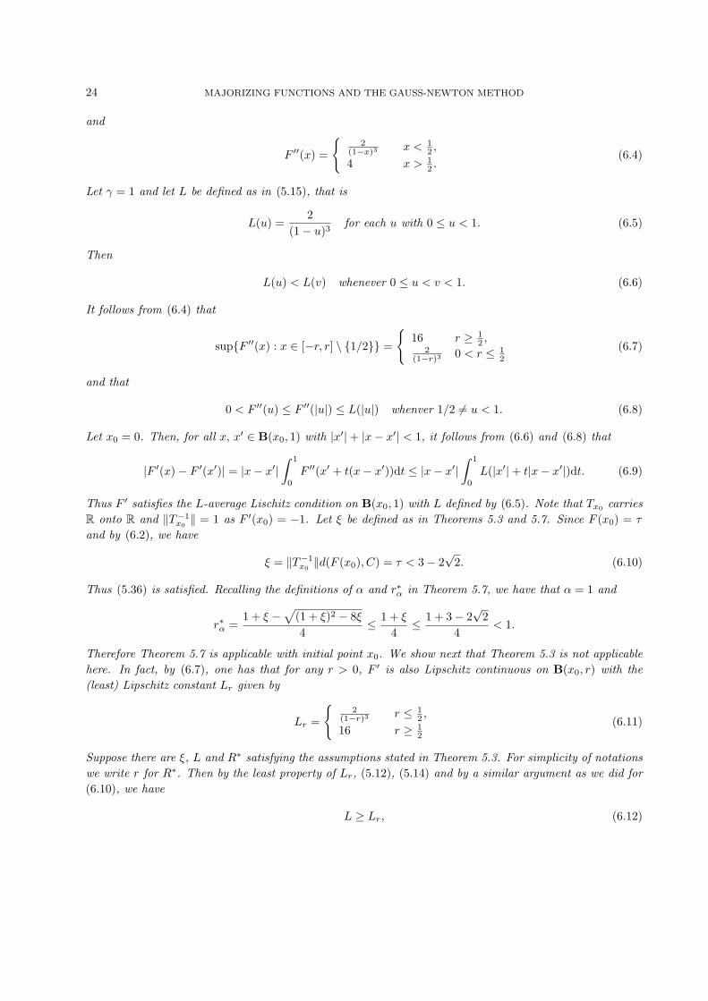
and
F ′′(x) =
{2
(1−x)3 x < 12 ,
4 x > 12 .
(6.4)
Let γ = 1 and let L be defined as in (5.15), that is
L(u) =2
(1− u)3for each u with 0 ≤ u < 1. (6.5)
Then
L(u) < L(v) whenever 0 ≤ u < v < 1. (6.6)
It follows from (6.4) that
sup{F ′′(x) : x ∈ [−r, r] \ {1/2}} =
{16 r ≥ 1
2 ,2
(1−r)3 0 < r ≤ 12
(6.7)
and that
0 < F ′′(u) ≤ F ′′(|u|) ≤ L(|u|) whenver 1/2 6= u < 1. (6.8)
Let x0 = 0. Then, for all x, x′ ∈ B(x0, 1) with |x′|+ |x− x′| < 1, it follows from (6.6) and (6.8) that
|F ′(x)− F ′(x′)| = |x− x′|∫ 1
0
F ′′(x′ + t(x− x′))dt ≤ |x− x′|∫ 1
0
L(|x′|+ t|x− x′|)dt. (6.9)
Thus F ′ satisfies the L-average Lischitz condition on B(x0, 1) with L defined by (6.5). Note that Tx0 carriesR onto R and ‖T−1
x0‖ = 1 as F ′(x0) = −1. Let ξ be defined as in Theorems 5.3 and 5.7. Since F (x0) = τ
and by (6.2), we have
ξ = ‖T−1x0‖d(F (x0), C) = τ < 3− 2
√2. (6.10)
Thus (5.36) is satisfied. Recalling the definitions of α and r∗α in Theorem 5.7, we have that α = 1 and
r∗α =1 + ξ −
√(1 + ξ)2 − 8ξ
4≤ 1 + ξ
4≤ 1 + 3− 2
√2
4< 1.
Therefore Theorem 5.7 is applicable with initial point x0. We show next that Theorem 5.3 is not applicablehere. In fact, by (6.7), one has that for any r > 0, F ′ is also Lipschitz continuous on B(x0, r) with the(least) Lipschitz constant Lr given by
Lr =
{2
(1−r)3 r ≤ 12 ,
16 r ≥ 12
(6.11)
Suppose there are ξ, L and R∗ satisfying the assumptions stated in Theorem 5.3. For simplicity of notationswe write r for R∗. Then by the least property of Lr, (5.12), (5.14) and by a similar argument as we did for(6.10), we have
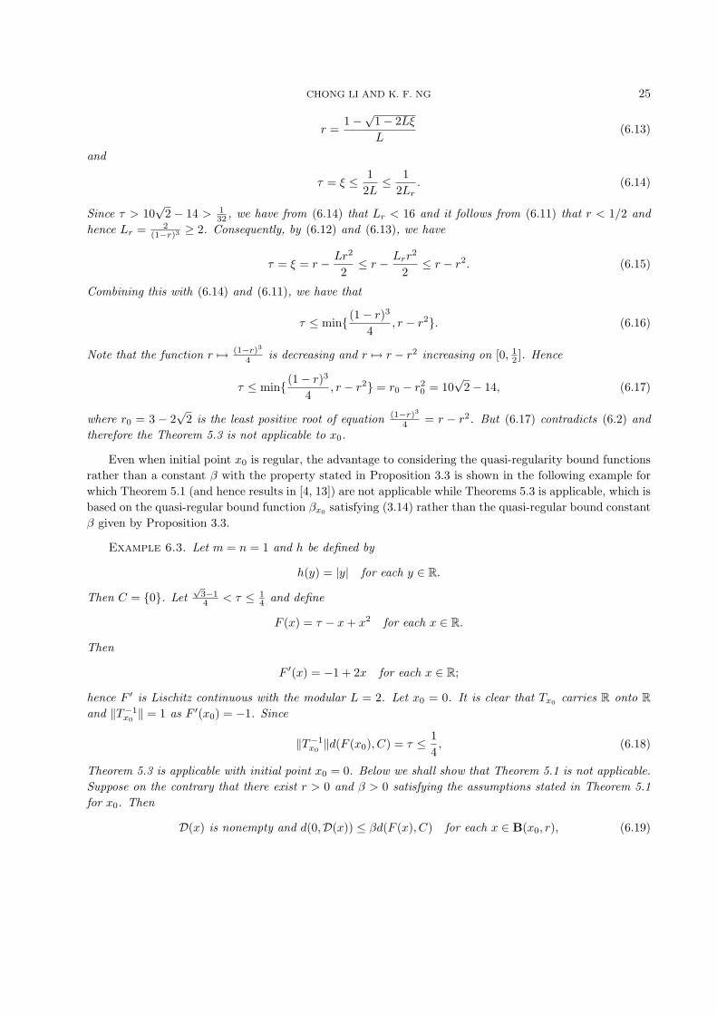
L ≥ Lr, (6.12)
CHONG LI AND K. F. NG 25
r =1−
√1− 2Lξ
L(6.13)
and
τ = ξ ≤ 12L
≤ 12Lr
. (6.14)
Since τ > 10√
2 − 14 > 132 , we have from (6.14) that Lr < 16 and it follows from (6.11) that r < 1/2 and
hence Lr = 2(1−r)3 ≥ 2. Consequently, by (6.12) and (6.13), we have
τ = ξ = r − Lr2
2≤ r − Lrr
2
2≤ r − r2. (6.15)
Combining this with (6.14) and (6.11), we have that
τ ≤ min{ (1− r)3
4, r − r2}. (6.16)
Note that the function r 7→ (1−r)3
4 is decreasing and r 7→ r − r2 increasing on [0, 12 ]. Hence
τ ≤ min{ (1− r)3
4, r − r2} = r0 − r2
0 = 10√
2− 14, (6.17)
where r0 = 3 − 2√
2 is the least positive root of equation (1−r)3
4 = r − r2. But (6.17) contradicts (6.2) andtherefore the Theorem 5.3 is not applicable to x0.
Even when initial point x0 is regular, the advantage to considering the quasi-regularity bound functionsrather than a constant β with the property stated in Proposition 3.3 is shown in the following example forwhich Theorem 5.1 (and hence results in [4, 13]) are not applicable while Theorems 5.3 is applicable, which isbased on the quasi-regular bound function βx0 satisfying (3.14) rather than the quasi-regular bound constantβ given by Proposition 3.3.
Example 6.3. Let m = n = 1 and h be defined by
h(y) = |y| for each y ∈ R.
Then C = {0}. Let√
3−14 < τ ≤ 1
4 and define
F (x) = τ − x + x2 for each x ∈ R.
Then
F ′(x) = −1 + 2x for each x ∈ R;
hence F ′ is Lischitz continuous with the modular L = 2. Let x0 = 0. It is clear that Tx0 carries R onto Rand ‖T−1
x0‖ = 1 as F ′(x0) = −1. Since
‖T−1x0‖d(F (x0), C) = τ ≤ 1
4, (6.18)
Theorem 5.3 is applicable with initial point x0 = 0. Below we shall show that Theorem 5.1 is not applicable.Suppose on the contrary that there exist r > 0 and β > 0 satisfying the assumptions stated in Theorem 5.1for x0. Then
D(x) is nonempty and d(0,D(x)) ≤ βd(F (x), C) for each x ∈ B(x0, r), (6.19)

26 MAJORIZING FUNCTIONS AND THE GAUSS-NEWTON METHOD
r ≥1 + 2βξ −
√1− (2βξ)2
2β(6.20)
and
βτ = ξ ≤ 12β
. (6.21)
By definitions, it is easy to see that, for each x ∈ R,
D(x) ={{−F ′(x)−1F (x)} x 6= 1
2 ,
∅ x = 12 .
(6.22)
and it follows from (6.19) that r ≤ 12 and for each x ∈ B(x0, r),
d(0,D(x)) = |F ′(x)−1F (x)| = 11− 2|x|
|F (x)| = 11− 2|x|
d(F (x), C). (6.23)
By (6.19) this implies that
11− 2|x|
≤ β for each x ∈ B(x0, r). (6.24)
Considering x0 = 0, this implies 11−2r ≤ β, that is,
2βr ≤ β − 1. (6.25)
It follows from (6.20) that
1 + 2βξ −√
1− (2βξ)2 ≤ β − 1, (6.26)
or equivalently,
((2ξ − 1)2 + (2ξ)2)β2 + 4(2ξ − 1)β + 3 ≤ 0. (6.27)
Hence
(4(2ξ − 1))2 − 4 · 3((2ξ − 1)2 + (2ξ)2) ≥ 0 (6.28)
which implies that ξ ≤√
3−14 . This contradicts the assumption that τ >
√3−14 because ξ = βτ ≥ τ by (6.21)
and (6.24).
We remark that, on one hand, the results in section 5 cover (and improve) the cases considered by Burke-Ferris and Robinson (the initial points are regular in [4, 18]), and on the other hand, there are examples ofquasi-regular but not regular points x0 for which Theorem 4.1 is applicable.
Example 6.4. Let m = n = 3. To ease our computation, let R3 be endowed with the l1-norm. Let h bedefined by
h(x) = χ(t1) + χ(t2) +∣∣∣∣t3 − t1 − t2 −
18
∣∣∣∣ for each x = (t1, t2, t3) ∈ R3,
where χ(t) is a real-valued function on R defined by
χ(t) =
−1− t t ≤ −10 −1 ≤ t ≤ 0t t ≥ 0.
CHONG LI AND K. F. NG 27
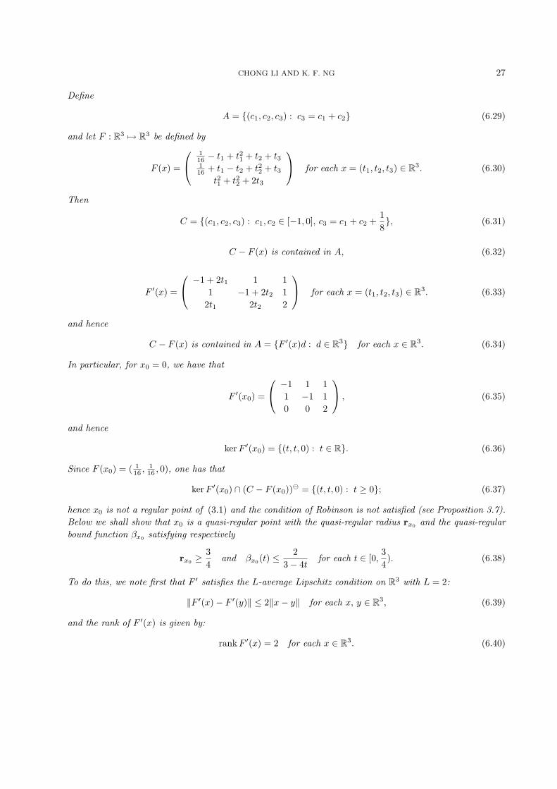
Define
A = {(c1, c2, c3) : c3 = c1 + c2} (6.29)
and let F : R3 7→ R3 be defined by
F (x) =
116 − t1 + t21 + t2 + t3116 + t1 − t2 + t22 + t3
t21 + t22 + 2t3
for each x = (t1, t2, t3) ∈ R3. (6.30)
Then
C = {(c1, c2, c3) : c1, c2 ∈ [−1, 0], c3 = c1 + c2 +18}, (6.31)
C − F (x) is contained in A, (6.32)
F ′(x) =
−1 + 2t1 1 11 −1 + 2t2 1
2t1 2t2 2
for each x = (t1, t2, t3) ∈ R3. (6.33)
and hence
C − F (x) is contained in A = {F ′(x)d : d ∈ R3} for each x ∈ R3. (6.34)
In particular, for x0 = 0, we have that
F ′(x0) =
−1 1 11 −1 10 0 2
, (6.35)
and hence
ker F ′(x0) = {(t, t, 0) : t ∈ R}. (6.36)
Since F (x0) = ( 116 , 1
16 , 0), one has that
ker F ′(x0) ∩ (C − F (x0)) = {(t, t, 0) : t ≥ 0}; (6.37)
hence x0 is not a regular point of (3.1) and the condition of Robinson is not satisfied (see Proposition 3.7).Below we shall show that x0 is a quasi-regular point with the quasi-regular radius rx0 and the quasi-regularbound function βx0 satisfying respectively
rx0 ≥34
and βx0(t) ≤2
3− 4tfor each t ∈ [0,
34). (6.38)
To do this, we note first that F ′ satisfies the L-average Lipschitz condition on R3 with L = 2:
‖F ′(x)− F ′(y)‖ ≤ 2‖x− y‖ for each x, y ∈ R3, (6.39)
and the rank of F ′(x) is given by:
rank F ′(x) = 2 for each x ∈ R3. (6.40)

28 MAJORIZING FUNCTIONS AND THE GAUSS-NEWTON METHOD
Since
F ′(x) = F ′(x0) + F ′(x)− F ′(x0) and ‖F ′(x)− F ′(x0)‖ ≤ 2‖x− x0‖,
it follows from the perturbation property of matrixes (cf. [27, 30]) that
‖F ′(x)†‖ ≤ ‖F ′(x0)†‖1− 2‖x− x0‖‖F ′(x0)†‖
(6.41)
holds for each x ∈ R3 with 2‖x−x0‖‖F ′(x0)†‖ < 1, where A† denotes the Moore-Penrose generalized inverseof the matrix A (cf. [27, 30]). By (6.35), one has that
F ′(x0)† =
− 14
14 0
14 − 1
4 016
16
13
and ‖F ′(x0)†‖ =23. (6.42)
This together with (6.41) implies that
‖F ′(x)†‖ ≤ 23− 4‖x− x0‖
for each x ∈ B(x0,34). (6.43)
On the other hand, by (6.33) and (3.2), we have
D(x) = F ′(x)†(C − F (x)) for each x ∈ R3 (6.44)
and, consequently, for each x ∈ B(x0,34 ),
d(0,D(x)) ≤ ‖F ′(x)†‖d(F (x), C) ≤ 23− 4‖x− x0‖
d(F (x), C). (6.45)
This shows that x0 is a quasi-regular point with the quasi-regular radius rx0 and the quasi-regular boundfunction βx0 satisfying (6.38). Let r = 3
4 . Recalling (4.2) and (6.1), it follows from (6.38) that
α0(r) ≤ sup{
β(t)β(t)2t + 1
: ξ ≤ t < r}
=23, (6.46)
where β(t) := 23−4t for each t ∈ [0, 3
4 ). Thus taking α = 23 in (2.1), we get that
rα =34
and bα =38. (6.47)
By (4.1) and (6.38),
ξ = βx0(0)d(F (x0), C) ≤ β(0)‖F (x0)− c0‖ =16,
where c0 = (0, 0, 18 ). It follows that (4.4) is satisfied. Hence Theorem 4.1 is applicable with initial point x0
even though it is not a regular point.

CHONG LI AND K. F. NG 29
7. Conclusion. In connection with inclusion problem (1.2) and for a given point x0 we introduce twonew notions: (a) the L-average Lipschitz condition for F ′ and (b) quasi-regularity (with the associate quasi-regular radius rx0 and quasi-regular bound function βx0). The notion (a) extends the classical Lipschitzcondition and Smale′s condition and notion (b) extends the regularity. When Robinson’s condition (3.12)is satisfied, x0 is shown to be a regular point and the associate quasi-regular radius rx0 as well as theassociate quasi-regular bound function βx0 are estimated if in addition F ′ satisfies (a) with suitable L. Weprovide sufficient conditions for convergence results with a quasi-regular initial point x0 in the Gauss-Newtonmethod for the convex composition optimization problem (1.1) with C given to be the set of all minimizersof a convex function h. These conditions are given in terms of rx0 , βx0 and L in the above (a). Examplesare given to show that the new concept and results are nontrivial extensions of the existing ones. We thankthe referees for suggestions which help our presentations.
REFERENCES
[1] J. M. Borwein, Stability and regular points of inequality systems, J. Optim. Theory Appl., 48(1986), pp. 9-52.
[2] J. V. Burke, Descent methods for composite nondifferentiable optimization problems, Math. programming, 33(3)(1985),
pp. 260-279.
[3] J. V. Burke, An exact penalization viewpoint of constrained optimization, SIAM J. Control Optim., 29(1991), pp. 968-998.
[4] J. V. Burke and M. C. Ferris, A Gauss-Newton method for convex composite optimization, Math. Programming,
71(1995), pp. 179-194.
[5] J. V. Burke and R. A. Poliquin, Optimality conditions for non-finite valued convex composite function, Math. Program-
ming, 57(1)(1992), pp. 103-120.
[6] R. Flecher, Second order correction for nondifferentiable optimization, in: G.A. Watson, ed. Numerical Analysis, Lecture
Notes in Mathematics, Vol.912 (Spring, Berlin, 1982), pp. 85-114.
[7] R. Flecher, Practical Methods of Optimization, Wiley, New York, 2nd ed. 1987.
[8] W. B. Gragg and R. A. Tapai, Optimal error bounds for the Newton-Kantorovich theorems, SIAM J. Numer. Anal.,
11(1974), pp. 10-13.
[9] J. Hiriart-Urruty and C. Lemarechal, Convex Analysis and Minimization Algorithms II, Vol. 305 of Grundlehren der
Mathematschen Wissenschaften, Springer, New York, 1993.
[10] K. Jittorntrum and M. R. Osborne, Strong uniqueness and second order convergence in nonlinear discrete approximation,
Numer. Math., 34(1980), pp. 439-455.
[11] L. V. Kantorovich, On Newton method for functional equations, Dokl. Acad. N USSR, 59(1948), pp. 1237-1240.
[12] L. V. Kantorovich and G. P. Akilov, Functional Analysis, New York: Pergamon Press, 1982.
[13] C. Li and X. H. Wang, On convergence of the Gauss-Newton method for convex composite optimization, Math. Pro-
gramming, 91(2002), pp. 349-356.
[14] W. Li and I. Singer, Global error bounds for convex multifunctions and applications, Math. Oper. Res., 23(1998), pp.
443–462.
[15] K. Madsen, Minimization of nonlinear approximation function, Ph.D.Thesis, Institute of Numerical Anakysis, Technical
University of Denmark, (Lyngby, 1985).
[16] K. F. Ng and X. Y. Zheng, Characterizations of error bounds for convex multifunctions on Banach spaces, Math. Oper.
Res., 29(2004), pp. 45–63.
[17] A. M. Ostrowski, Solutions of Equations in Euclidean and Banach Spaces, Academic Press, New York, 1973.
[18] S. M. Robinson, Extension of Newton′s method to nonlinear function with values in cone, Numer. Math., 19(1972), pp.
341-347.
[19] S. M. Robinson, Normed convex process, Trans. Amer. Math. Soc., 174(1972), pp. 127-140.
[20] S. M. Robinson, Stability theory for systems of inequalities, Part I: Linear systems, SIAM J. Nume. Anal., 12(1975),
pp. 754-769.
[21] S. M. Robinson, Stability theory for systems of inequalities, Part II: Differentiable nonlinear systems, SIAM J. Nume.
Anal., 13(1976), pp. 479-513.
[22] R. T. Rockafellar, First and second order epi-differentiability in nonlinear programming, Trans. Amer. Math. Soc.,
307(1988), pp. 75-108.
[23] R. T. Rockafellar, Convex Analysis, Princeton University Press, Princeton, NJ. 1970.
[24] R. T. Rockafellar, Monotone processes of convex and concave type, Amer. Math. Soc. Memoir, 77(1967).

30 MAJORIZING FUNCTIONS AND THE GAUSS-NEWTON METHOD
[25] R. T. Rockafellar, First- and second-order epi-differentiability in nonlinear programming, Trans. Amer. Math. Soc.,
307(1988), pp. 75-108.
[26] S. Smale, Newton′s method estimates from data at one point, The Merging of Disciplines: New Directions in Pure,
Applied and Computational Mathematics (R.Ewing, K.Gross and C. Martin, eds), New York: Springer, 1986, pp.
185-196.
[27] G. Stewart, On the continuity of the generalized inverse, SIAM J. Appl. Math., 17(1960), 33-45.
[28] X. H. Wang, Convergence of Newton′s method and inverse function theorem in Banach space, Math. Comp., 68(1999),
pp. 169-186.
[29] X. H. Wang, Convergence of an iteration process, KeXue Tongbao, 20(1975), pp. 558-559.
[30] P. Wedin, Perturbation theory for pseudo-inverse, BIT, 13(1973), pp. 217-232.
[31] R. S. Womersley, Local properties of algorithms for minimizing nonsmooth composite function, Math. Programming,
32(1985), pp. 69-89
Related Documents