WILLEM VAN JAARSVELD Maintenance Centered Service Parts Inventory Control brought to you by C provided by Erasmus University Digital Repo

Welcome message from author
This document is posted to help you gain knowledge. Please leave a comment to let me know what you think about it! Share it to your friends and learn new things together.
Transcript

WILLEM VAN JAARSVELD
Maintenance CenteredService Parts InventoryControl
WILLE
M VAN JA
ARSVELD
- Maintenance Centered Service
Parts In
ventory Contro
l
ERIM PhD SeriesResearch in Management
Erasm
us Research Institute of Management-
288
ER
IM
De
sig
n &
la
you
t: B
&T
On
twe
rp e
n a
dvi
es
(w
ww
.b-e
n-t
.nl)
Pri
nt:
Ha
vek
a
(w
ww
.ha
vek
a.n
l)MAINTENANCE CENTERED SERVICE PARTS INVENTORY CONTROL
High-tech capital goods enable the production of many services and articles that havebecome a part of our daily lives. Examples include the refineries that produce the gasolinewe put in our cars, the photolithography systems that enable the production of the chipsin our cell phones and laptops, the trains and railway infrastructure that facilitate publictransport and the aircraft that permit us to travel long distances. To prevent costlyproduction disruptions of such systems when failures occur, it is crucial that service partsare readily available to replace any failed parts. However, service parts representsignificant investments and failures are unpredictable, so it is unclear which parts shouldbe stocked and in what quantity.
In this thesis, analytical models and solution methods are developed to aid companiesin making this decision. Amongst other things, we analyze systems in which multiple partsneed replacement after a failure, a situation that is frequently encountered in practice.This affects the ability to complete repairs in a timely fashion. We develop new modelingtechniques in order to apply scalable deterministic approaches, such as column generationtechniques and sample average approximation methods, to the problem. This leads tosolution techniques that, unlike traditional methods, can ensure that all parts needed tocomplete maintenance are readily available. The approach is capable of meeting thechallenging requirements of a real-life repair shop.
The Erasmus Research Institute of Management (ERIM) is the Research School (Onder -zoek school) in the field of management of the Erasmus University Rotterdam. The foundingparticipants of ERIM are the Rotterdam School of Management (RSM), and the ErasmusSchool of Econo mics (ESE). ERIM was founded in 1999 and is officially accre dited by theRoyal Netherlands Academy of Arts and Sciences (KNAW). The research under taken byERIM is focused on the management of the firm in its environment, its intra- and interfirmrelations, and its busi ness processes in their interdependent connections.
The objective of ERIM is to carry out first rate research in manage ment, and to offer anad vanced doctoral pro gramme in Research in Management. Within ERIM, over threehundred senior researchers and PhD candidates are active in the different research pro -grammes. From a variety of acade mic backgrounds and expertises, the ERIM commu nity isunited in striving for excellence and working at the fore front of creating new businessknowledge.
Erasmus Research Institute of Management - Rotterdam School of Management (RSM)Erasmus School of Economics (ESE)Erasmus University Rotterdam (EUR)P.O. Box 1738, 3000 DR Rotterdam, The Netherlands
Tel. +31 10 408 11 82Fax +31 10 408 96 40E-mail [email protected] www.erim.eur.nl
Mon Apr 15 2013 - B&T13181_ERIM_Omslag_Jaarsveld_15April13.pdf
brought to you by COREView metadata, citation and similar papers at core.ac.uk
provided by Erasmus University Digital Repository

Maintenance Centered
Service Parts Inventory Control

Maintenance Centered
Service Parts Inventory Control
Onderhoudsgericht voorraadbeheer van reservedelen
Thesis
to obtain the degree of Doctor from the
Erasmus University Rotterdam
by command of the
rector magnificus
Prof.dr. H.G. Schmidt
and in accordance with the decision of the Doctorate Board.
The public defense shall be held on
Thursday 30 May 2013 at 15:30 hours
by
Willem Leendert van Jaarsveld
born in Sint-Oedenrode, the Netherlands.

Doctoral Committee
Promotor: Prof.dr.ir. R. Dekker
Other members: Dr. E. van der Laan
Prof.dr. R.H. Teunter
Prof.dr.ir. G.J.J.A.N. van Houtum
Erasmus Research Institute of Management - ERIM
The joint research institute of the Rotterdam School of Management (RSM)
and the Erasmus School of Economics (ESE) at the Erasmus University Rotterdam
Internet: http://www.erim.eur.nl
ERIM Electronic Series Portal: http://hdl.handle.net/1765/1
ERIM PhD Series in Research in Management, 288
ERIM reference number: EPS-2013-288-LIS
ISBN 978-90-5892-332-5c©2013, Willem van Jaarsveld
Design: B&T Ontwerp en advies www.b-en-t.nl
This publication (cover and interior) is printed by haveka.nl on recycled paper, Revive R©.
The ink used is produced from renewable resources and alcohol free fountain solution.
Certifications for the paper and the printing production process: Recycle, EU Flower, FSC, ISO14001.
More info: http://www.haveka.nl/greening
All rights reserved. No part of this publication may be reproduced or transmitted in any form or by any means electronic
or mechanical, including photocopying, recording, or by any information storage and retrieval system, without permission
in writing from the author.

Acknowledgments
This thesis is the result of a project that I have been working on during the past five years.
I would like to take this opportunity to thank the many people that have contributed to
this thesis.
First, I want to express my gratitude to my supervisor Rommert Dekker. I thank you
for giving me the opportunity to start this project, for all the ideas and advice you gave
me during the project, and most of all for encouraging and enabling me to collaborate
with companies in applied research. Seeing my research being applied in practice has
been a very inspiring and motivating experience.
I am grateful to Fokker Services, and in particular to Cors van der Laan, for giving
me several opportunities to engage in projects that enabled me to apply my research.
These projects have been my primary motivation for engaging in the research presented
in Chapters 2, 3, 4 and 6 of this thesis. I thank all employees of Fokker Services that made
these projects possible by giving me their insights, support, and advice. I am particularly
grateful to Martin de Jong, Cors van der Laan, Maarten van Marle and Ed Wannee for
all the support and guidance they gave me during these projects. I thank Bart van Hees
and Harry van Teijlingen of Shell Global Solutions for the opportunity for joint research
and for their valuable input that has formed the basis for Chapter 5. I also thank SLF
Research and ProSeLo for providing an inspiring environment for applying research in
practice.
I am grateful to Ward Romeijnders and Ruud Teunter of the University of Groningen
for our joint work, which led to Chapter 4. I am happy that Ruud agreed to be a part
of my inner committee. I am also indebted to the other members of my inner committee,
Geert-Jan van Houtum and Erwin van der Laan, for the time they spent to evaluate the
thesis. In addition, I want to thank Geert-Jan for his valuable feedback on preliminary
drafts of chapters of this thesis. I am thankful to Matthieu van der Heijden, Rene de
Koster, Alan Scheller-Wolf, and Albert Wagelmans for being a member of my doctoral
committee.

vi Acknowledgments
From April to July 2012, I visited Alan Scheller-Wolf at Carnegie Mellon University.
I thank Alan for his hospitality, and for our cooperation during this period, that led to
the research presented in Chapter 3. I thank the PhD students in the Tepper School
for showing me around in Pittsburgh, and for the enjoyable time I had with them in
Pittsburgh.
I thank my colleagues Twan, Remy, Kristiaan, Mathijn, Judith, Zahra, Ilse and Lanah
for sharing their research problems and insights during our joint lunches and coffee breaks.
It is inspiring to work with enthusiastic people like you. Twan, I thank you for our
collaboration which led to the algorithms described in Chapter 2, for your valuable advice
on all aspects of being a PhD student, and for agreeing to stand by my side as one of my
paranymphs. I thank Remy for organizing the lecture series about stochastic programming
in early 2011, which has been an inspiration for the research presented in Chapter 3. In
addition, I thank all colleagues who joined the Friday afternoon drinks, dinners, and
sports activities for the good times we had together.
I want to thank my friends and family for being interested in this project, but mostly
for helping me to take my mind off the project every now and then. I am especially
thankful to my parents, sister, and brothers for their love and support. Corneel, I am
very happy that you also agreed to be one of my paranymphs. Finally, I wish to thank
my partner. Eva, my deepest word of thanks goes to you, for your support and love
throughout this project.
Willem van Jaarsveld
Utrecht, March 2013
Contents
Acknowledgments v
1 Introduction 1
1.1 Capital goods . . . . . . . . . . . . . . . . . . . . . . . . . . . . . . . . . . 1
1.2 Maintenance . . . . . . . . . . . . . . . . . . . . . . . . . . . . . . . . . . . 2
1.3 Service parts inventories . . . . . . . . . . . . . . . . . . . . . . . . . . . . 4
1.4 Motivation . . . . . . . . . . . . . . . . . . . . . . . . . . . . . . . . . . . . 6
1.5 Outline of this thesis . . . . . . . . . . . . . . . . . . . . . . . . . . . . . . 8
2 Spare parts inventory control for an aircraft component repair shop 11
2.1 Introduction . . . . . . . . . . . . . . . . . . . . . . . . . . . . . . . . . . . 11
2.2 Literature review . . . . . . . . . . . . . . . . . . . . . . . . . . . . . . . . 14
2.3 The optimization problem . . . . . . . . . . . . . . . . . . . . . . . . . . . 17
2.3.1 The model . . . . . . . . . . . . . . . . . . . . . . . . . . . . . . . . 17
2.3.2 Bounds on performance measures . . . . . . . . . . . . . . . . . . . 19
2.3.3 Cost minimization under fill rate constraints . . . . . . . . . . . . . 21
2.3.4 The pricing problem . . . . . . . . . . . . . . . . . . . . . . . . . . 23
2.4 The algorithm . . . . . . . . . . . . . . . . . . . . . . . . . . . . . . . . . . 24
2.4.1 Column generation algorithm . . . . . . . . . . . . . . . . . . . . . 24
2.4.2 Algorithm for the pricing problem . . . . . . . . . . . . . . . . . . . 25
2.4.3 Finding integer solutions . . . . . . . . . . . . . . . . . . . . . . . . 29
2.5 Computational results . . . . . . . . . . . . . . . . . . . . . . . . . . . . . 31
2.6 Case study . . . . . . . . . . . . . . . . . . . . . . . . . . . . . . . . . . . . 32
2.7 Conclusion . . . . . . . . . . . . . . . . . . . . . . . . . . . . . . . . . . . . 38
2.A Proof of propositions . . . . . . . . . . . . . . . . . . . . . . . . . . . . . . 39
3 Optimization of industrial-scale assemble-to-order systems 43
3.1 Introduction . . . . . . . . . . . . . . . . . . . . . . . . . . . . . . . . . . . 44
3.2 Literature review . . . . . . . . . . . . . . . . . . . . . . . . . . . . . . . . 47
viii Contents
3.3 Methods . . . . . . . . . . . . . . . . . . . . . . . . . . . . . . . . . . . . . 51
3.3.1 Model and preliminaries . . . . . . . . . . . . . . . . . . . . . . . . 51
3.3.2 Base-stock levels under FCFS . . . . . . . . . . . . . . . . . . . . . 53
3.3.3 A lower bound on the costs under optimal allocation . . . . . . . . 58
3.4 Results . . . . . . . . . . . . . . . . . . . . . . . . . . . . . . . . . . . . . . 59
3.4.1 The investigated policies . . . . . . . . . . . . . . . . . . . . . . . . 60
3.4.2 PC assembly case . . . . . . . . . . . . . . . . . . . . . . . . . . . . 62
3.4.3 Maintenance Organisation . . . . . . . . . . . . . . . . . . . . . . . 64
3.4.4 Assembly of products of multiple families . . . . . . . . . . . . . . . 66
3.4.5 Discussion . . . . . . . . . . . . . . . . . . . . . . . . . . . . . . . . 69
3.5 Conclusions and future research . . . . . . . . . . . . . . . . . . . . . . . . 71
3.A Sample generation . . . . . . . . . . . . . . . . . . . . . . . . . . . . . . . 72
3.B Proof of propositions . . . . . . . . . . . . . . . . . . . . . . . . . . . . . . 73
3.C Data for the maintenance organization problem . . . . . . . . . . . . . . . 74
4 Forecasting Spare Parts Demand using Information on Component Re-
pairs 77
4.1 Introduction . . . . . . . . . . . . . . . . . . . . . . . . . . . . . . . . . . . 77
4.2 Literature review . . . . . . . . . . . . . . . . . . . . . . . . . . . . . . . . 79
4.3 Data description . . . . . . . . . . . . . . . . . . . . . . . . . . . . . . . . 80
4.4 Forecasting methods . . . . . . . . . . . . . . . . . . . . . . . . . . . . . . 81
4.4.1 Initialization of the forecasting methods . . . . . . . . . . . . . . . 86
4.5 Results for case study . . . . . . . . . . . . . . . . . . . . . . . . . . . . . 87
4.6 General results . . . . . . . . . . . . . . . . . . . . . . . . . . . . . . . . . 90
4.6.1 Stationary demand: analytical results . . . . . . . . . . . . . . . . . 91
4.6.2 Stationary and non-stationary demand: simulation results . . . . . 92
4.7 Conclusions . . . . . . . . . . . . . . . . . . . . . . . . . . . . . . . . . . . 93
5 Spare parts stock control for redundant systems using RCM data 95
5.1 Introduction . . . . . . . . . . . . . . . . . . . . . . . . . . . . . . . . . . . 95
5.2 Problem setting . . . . . . . . . . . . . . . . . . . . . . . . . . . . . . . . . 100
5.2.1 The RCM data . . . . . . . . . . . . . . . . . . . . . . . . . . . . . 100
5.2.2 Model requirements . . . . . . . . . . . . . . . . . . . . . . . . . . . 101
5.3 The model . . . . . . . . . . . . . . . . . . . . . . . . . . . . . . . . . . . . 102
5.3.1 Formal description . . . . . . . . . . . . . . . . . . . . . . . . . . . 103
5.3.2 Motivation . . . . . . . . . . . . . . . . . . . . . . . . . . . . . . . . 104
5.4 Approximate analysis . . . . . . . . . . . . . . . . . . . . . . . . . . . . . . 105
Contents ix
5.4.1 The downtime costs for fixed total repair time . . . . . . . . . . . . 106
5.4.2 Approximating the downtime costs . . . . . . . . . . . . . . . . . . 107
5.4.3 Optimization . . . . . . . . . . . . . . . . . . . . . . . . . . . . . . 110
5.4.4 Traditional inventory methods . . . . . . . . . . . . . . . . . . . . . 111
5.5 Setup of simulation experiment . . . . . . . . . . . . . . . . . . . . . . . . 111
5.5.1 Simulation . . . . . . . . . . . . . . . . . . . . . . . . . . . . . . . . 111
5.5.2 Cases . . . . . . . . . . . . . . . . . . . . . . . . . . . . . . . . . . . 113
5.6 Results & discussion . . . . . . . . . . . . . . . . . . . . . . . . . . . . . . 115
5.6.1 Computation times . . . . . . . . . . . . . . . . . . . . . . . . . . . 115
5.6.2 Precision of downtime cost approximations . . . . . . . . . . . . . . 116
5.6.3 Deviations from the true optimum . . . . . . . . . . . . . . . . . . . 117
5.6.4 Cost impact . . . . . . . . . . . . . . . . . . . . . . . . . . . . . . . 118
5.7 Conclusions . . . . . . . . . . . . . . . . . . . . . . . . . . . . . . . . . . . 121
6 Estimating obsolescence risk from demand data - A case study 123
6.1 Introduction . . . . . . . . . . . . . . . . . . . . . . . . . . . . . . . . . . . 123
6.2 Obsolescence of service parts . . . . . . . . . . . . . . . . . . . . . . . . . . 125
6.2.1 Dead stock . . . . . . . . . . . . . . . . . . . . . . . . . . . . . . . 126
6.2.2 Demand non-stationarity . . . . . . . . . . . . . . . . . . . . . . . . 127
6.3 Analysis of service part demand data . . . . . . . . . . . . . . . . . . . . . 129
6.4 The method . . . . . . . . . . . . . . . . . . . . . . . . . . . . . . . . . . . 134
6.4.1 Modeling discussion . . . . . . . . . . . . . . . . . . . . . . . . . . . 134
6.5 Conclusions and extensions . . . . . . . . . . . . . . . . . . . . . . . . . . . 144
7 Optimizing (S − 1, S) inventory models with multiple demand classes 145
7.1 Introduction . . . . . . . . . . . . . . . . . . . . . . . . . . . . . . . . . . . 145
7.2 The model . . . . . . . . . . . . . . . . . . . . . . . . . . . . . . . . . . . . 147
7.3 Existing theory . . . . . . . . . . . . . . . . . . . . . . . . . . . . . . . . . 149
7.4 Optimality of the algorithms . . . . . . . . . . . . . . . . . . . . . . . . . . 151
7.5 Extensions . . . . . . . . . . . . . . . . . . . . . . . . . . . . . . . . . . . . 159
7.6 Conclusions . . . . . . . . . . . . . . . . . . . . . . . . . . . . . . . . . . . 161
8 Summary and Conclusions 163
References 169
Nederlandse Samenvatting (Summary in Dutch) 181
About the author 187

Chapter 1
Introduction
1.1 Capital goods
High-tech capital goods enable the production of many services and articles that have
become a part of our daily lives. Examples include the refineries that produce the gasoline
that enables us to use private transport, the photolithography systems that enable the
production of the chips in our cell phones and laptops, the trains and railway infrastructure
that facilitate public transport, and the aircraft that permit us to travel long distances.
High-tech capital goods consist of hundreds or thousands of components that interact
in a complex manner. Engineering, manufacturing, operating, and maintaining them are
therefore knowledge and labor intensive tasks. These expenses can only be justified by the
large output of capital goods. Each day for example, a crude oil distillation unit produces
hundreds of thousands of liters of gasoline, a photolithography system manufactures tens
of thousands of chips, and a single train or aircraft may transport thousands of travelers.
However, to produce large outputs of the desired quality efficiently, the operation needs
to be planned and executed effectively. The large potential output of capital goods, and
the significant investment which they represent, explain why periods in which the capital
good is not available for production (downtime) are very undesirable. During downtime,
potential production is being lost, and the investment in the capital good is not paying
off. When downtime is unforeseen because of a sudden breakdown, the consequences are
often much more severe. In particular, significant disruptions in the operational execution
occur because the operational planning is relying on the capital good being available. This
may result in loss of service and idle time for other resources, in addition to the loss of
production. In some cases, unforeseen downtime may also cause safety hazards. For
example, when an aircraft has unplanned downtime at the gate its planned flight has to
be postponed: Passengers are delayed, which may result in missed connections causing
2 Introduction
further delays and empty seats; the take-off and landing slots allocated to the flight are
lost, causing still further delays and possible disruptions; the crew for the flight sits idle,
etc. The costs of such a situation are estimated in the order of e30, 000/hr (Knotts,
1999). Of course, downtime may have even more pressing consequences while the aircraft
is airborne.
1.2 Maintenance
To reduce downtime, the capital good has to be properly maintained. In recent years,
effective and efficient maintenance has gained importance as a consequence of increasing
customer expectations, redoubled efforts to efficiently utilize the capital goods, and stricter
safety regulations. For instance, (low-cost) airliners can only operate profitably despite
low fares by assuring high fleet utilization; the Netherlands Railways are under more
and more pressure to assure availability of train services even if cold weather causes
technical difficulties in rolling stock and railway infrastructure; and crude oil refineries
and microelectronics plants need to constantly increase output to remain competitive. In
addition, both airliners and oil refineries need to adhere to ever stricter safety regulations.
As a consequence of the need to make maintenance effective and efficient, the manner
in which it is organized is changing. For many aspects of maintenance, the operators
depend on the original equipment manufacturers (OEMs) of the capital good. Increas-
ingly, this leads operators to take into account the OEMs ability to provide after-sales
service when procuring the capital good. Because of this development, the OEMs are
no longer competing only on the price and specifications of the equipment they produce,
but also on their ability to aid the operator in efficiently maintaining the equipment.
OEMs are responding by shifting attention to their after-sales service, which is all the
more attractive because after-sales profit margins are often much higher than the margins
when selling the capital good (Deloitte, 2006). As a consequence, the responsibility to
prevent downtime is in many cases shifting from the operator towards OEMs. The OEM
may provide guarantees for availability of service parts, and they may even go as far as
performing maintenance for the operator, taking full responsibility for the availability of
the capital good. Moreover, the high profit margins in after-sales have induced many
operator-affiliated and third-party maintenance organizations to sell their services on the
market. This has increased the pressure on all parties active in this market to perform
maintenance as efficiently as possible, which has redoubled interest in ideas that can cost-
efficiently reduce downtime. An important development in this direction, which is the
1.2 Maintenance 3
main focus of this thesis, is the application of decision support systems for service parts
inventory control.
We next summarize the methods used by maintenance organizations to reduce down-
time. The first method, aimed at reducing unplanned downtime, is to assign periods in
advance for carrying out (preventive) maintenance, in order to reduce the likelihood that
the capital good fails while the operational planning is relying on it. However, because
the period assigned to maintenance is (planned) downtime itself, the maintenance needs
to be fast and efficient: It should reduce the risk of unplanned downtime to an acceptable
level as quickly as possible without excessive use of resources. A second method to re-
duce downtime, which augments the first method, is to repair the capital good as quickly
as possible when unplanned downtime does occur in spite of maintenance. Repair may
be referred to as corrective maintenance to emphasize that repair and maintenance are
similar in character.
To assure that maintenance is efficient, a detailed maintenance schedule is typically
drawn up for the capital good, consisting of tasks that need to be carried out periodically.
When the capital good is down for maintenance, a number of such tasks are carried out
simultaneously/in rapid succession. Depending on the number of tasks that are planned to
be executed, a certain amount of downtime is planned, after which production is planned
to resume again. It is the task of the maintenance organization to complete all tasks in the
time that is designated for the maintenance. Maintenance tasks include activities such as
lubrication, cleaning, adjustment, and replacement of parts of the capital good. Parts are
typically replaced because evidence indicates that they are malfunctioning/might start
malfunctioning soon. Such evidence may be based on inspections, measurements, or on
the time since the part was installed in the capital good.
Parts may be relatively simple (for example bolts, nuts, seals, resistors), in which case
the replacement part is typically newly manufactured and the removed part is discarded.
However, parts replaced during maintenance of the capital good may also be complex
components, which can be maintained themselves. In fact, capital goods are increasingly
designed to consist of such components that can be replaced relatively easily. This de-
sign has the advantage that maintenance of the components need not be carried out at
the same location as the maintenance of the capital good. It can be performed by ded-
icated component repair shops or back-shops. This allows a few locations to specialize
in repairing specific types of components, which reduces investment in staff training and
test equipment, because such investments need to be made at less locations and for less
employees.
4 Introduction
Similar to maintenance of the capital good, component maintenance is streamlined
by constructing a detailed maintenance planning that summarizes all maintenance tasks
that need to be carried out on the component. During many such tasks, parts of the
component that are causing malfunction, or that may cause a malfunction soon, are
replaced. Because these parts are replaced at a repair shop, they are often referred to as
shop-replacable parts.
1.3 Service parts inventories
To reduce the time needed for repair or maintenance of the capital good, organizations
typically keep an exchange stock of spare components. These spares can be used to replace
a component during maintenance or repair of the capital good. After maintenance, the
removed components are added to the exchange stock again. This keeps the downtime of
the capital good limited, because it can resume production while the removed components
are still being maintained. Similarly, spare components facilitate rapid repairs of the
capital good.
To reduce the amount of capital invested in service parts, maintenance organizations
are reducing the amount of spare components kept in stock. This has increased the impor-
tance of assuring a short component repair turnaround time (TAT): The interval between
removing the component from the capital good and completing the maintenance of the
component. Short TATs assure that components become available for future maintenance
of the capital good as soon as possible. When no spare components are available at all,
completion of maintenance of the capital goods depends directly on component TATs,
which further increases their importance. The increasing importance of short component
TATs puts pressure on repair shops to assure that repair resources are carefully managed
to assure their timely availability, without running excessive costs. Key repair resources
are staff that is qualified to conduct the repair, tools, test equipment, and the parts that
need to be replaced.
Inventories of components and parts are typically designated as service parts invento-
ries. The previous discussions reveal that sufficient service parts inventories are critical to
prevent downtime, and short downtimes are essential for the profitability of companies.
However, service parts inventories are very costly. For example, service parts expenditures
in the US are estimated to constitute eight percent of their gross domestic product (GDP)
(Jasper, 2006). Service parts related expenditures may constitute an even larger fraction
of GDP in the Netherlands, because relatively many multinational companies (including
many Dutch multi-nationals) have their European distribution center for service parts
1.3 Service parts inventories 5
located in the Netherlands. The importance of service parts availability is increasing the
strategic importance of service parts inventory management. Indeed, in answer to the
question “how important is the efficient and effective management of service parts to
the overall success of your company?”, three quarters of supply and operations managers
answered very important or critical (AberdeenGroup, 2005).
The enormous expenditure constituted by service parts inventories is caused by a
number of properties of capital goods. First, the need for service parts is highly uncertain,
because in general it is very hard to predict which service parts will need replacement
in future maintenance or repairs. To reduce the risk of downtime of the capital good,
inventory is thus kept for all components/parts that might fail, implying that a very
broad assortment is needed because capital goods consist of many different components,
each consisting of many parts. Typical service parts inventories consists of 5000-20000
different service parts. Such a broad assortment constitutes a significant investment,
especially because manufacturing of service parts is costly because of the use of advanced
technologies, high quality standards, and low production volumes. Additional costs may
occur when components (or entire capital goods) are superseded because of changing
technologies. In those cases, the related service parts inventories become obsolete, and
need to be scrapped or otherwise dealt with.
Arriving at proper inventory decisions is a difficult task for human decision makers,
because they need to balance the objective to reduce the risk of stock-outs, and the
objective to control inventory costs. When decision makers are mainly responsible for
only one of these aspects, this may lead to non-optimal choices. For instance, engineers
that are responsible for the continued operation of a crude oil distillation unit may be
tempted to overstock on service parts. On the other hand, a manager that has the
target to increase stock turns may be tempted to understock, causing significant losses
resulting from the decreasing operational availability of the capital goods. And even if
decision makers are responsible for both objectives, difficulties may still arise. Without a
quantification of the relative importance of both objectives, decision makers can only act
on their subjective perception of those priorities, resulting in inefficient inventory control.
However, developing such a quantification involves estimating the cost of service parts
shortages, and the costs of holding inventory. The costs of service parts shortages is
related to the costs of downtime. However, the precise relation may be hard to quantify,
especially if the capital good has built-in redundancy. When maintenance tasks/service
parts are supplied to external (or internal) customers that operate the capital good,
then the costs of downtime are often only the secondary motive to avoid service parts
shortages. In those cases, the primary motive to avoid shortages is the need to meet
6 Introduction
(formal or informal) agreements with customers, in order to remain in business. If made
explicit, such agreements are typically expressed in terms of service level targets. However,
setting appropriate targets is challenging. Finally, to estimate the annual costs of holding
inventory, simple rules are in use. Typically, a percentage of 20-30% of the value of the
service part is used. However, such an approach may be too basic when the risk of parts
becoming obsolete is an important factor.
Another challenge arises when multiple tasks need to be carried out to complete the
maintenance, for instance when a capital good is down for planned maintenance, or in
the case of component maintenance. In those cases, multiple service parts need to be
available to complete the maintenance. This makes it even more difficult to assess the
operational costs of service parts shortages, because delays of the maintenance may be
caused by shortages of multiple different parts.
1.4 Motivation
This thesis addresses the challenges of service parts inventory control by developing an-
alytic models. Those models are used to gain insights into the interplay between the
different aspects of service parts inventories and the strategies for controlling those in-
ventories. In addition, analytic models of service parts inventory control can be used as
the basis for decision support software, to directly aid companies in making the right
decision. The difficulties discussed in the previous section show that decision makers in
companies can benefit from such decision support systems, especially because they only
have limited time to control inventory of hundreds or thousands of service parts. Indeed,
decision support systems are becoming ever more prevalent in practice, as a consequence
of the increasing importance of cost-efficient maintenance. In addition, the applicability
of such systems has benefited from the large amounts of data that are available in modern
ERP systems.
However, some aspects of service parts inventory control are difficult to model in a
computationally tractable manner. Furthermore, it is not clear how to estimate parame-
ters such as downtime costs and obsolescence risk. This thesis develops approaches based
on analytic models to overcome these difficulties.
The use of analytic models to gain insights into service parts inventories and to support
practitioners in making the right decision is well established. Indeed, the research in
this thesis builds on the work of other scholars. A review of the literature related to
the research presented in Chapters 2-7 is available in the literature and/or introduction
section of the chapters.
1.4 Motivation 7
The problems and inefficiencies in the service supply chain has long been the topic
of the Service Logistics Forum, a cooperation initiated by Districon Consultants where
companies exchange ideas about the service chain. In early 2000, a research project called
SLF research was started from this forum, involving TU Eindhoven, University of Twente
an Erasmus University, and some 9 companies on service logistics topics. Several of these
companies played a major role in the research presented in this thesis.
We next discuss the direct practical motivation for the work presented in this thesis.
The model and methods discussed in Chapter 2 result from a close collaboration of the
author with a repair shop owned by Fokker Services. The modeling is based on interviews
and in-depth discussions with employees of the company, and has undergone several en-
hancements over a period of several years to improve usability. The model and methods
have been implemented by the author as a decision support tool that is currently being
used by the company. Section 2.6 of this thesis presents quotes, analysis, and discussions
that reveal that this tool has a significant positive impact on the ability of the company
to cost efficiently attain business targets with respect to repair turnaround times. Discus-
sions at a repair shop owned by NedTrain have revealed that the approach is likely to be
beneficial for other repair shops as well (Aerts, 2012). In Chapters 3 and 4 we investigate
important practical questions pertaining the decision support tool developed in Chapter 2.
In particular, we investigate the impact of modeling assumptions underpinning the tool,
and the performance of a certain type of forecasting method that is used in the tool.
The model and approximative method described in Chapter 5 are the outcome of a
collaboration with a large petrochemical company, and resulted in an enhanced stocking
rule for the company. The method has also led to a better understanding of the role of
spare parts inventories for redundant systems at the company (cf. Van Jaarsveld and
Dekker, 2009). The research in Chapter 6 is motivated by discussions at an OEM of long
life-cycle products, during which employees of the company revealed their suspicions that
slow moving parts have a larger risk of becoming obsolete. We give evidence confirming
this theory. To incorporate the risk of obsolescence into a decision support tool that we
were developing for the company, we developed methods capable of quantifying the risk
of obsolescence. The resulting decision support tool is currently being used by the com-
pany. Table 6.3 illustrates how incorporating the risk of obsolescence enhances inventory
decisions.
8 Introduction
1.5 Outline of this thesis
In Chapters 2, 3 and 4 we explore different aspects of inventory control when maintenance
requires a number of different spare parts simultaneously to complete. This is typically
the case in practice, especially for component maintenance and planned maintenance of
capital goods. However, analytic models for spare parts are typically based on the as-
sumption that only a single part is needed to complete maintenance (e.g. Sherbrooke,
1968; Muckstadt, 1973; Rustenburg et al., 2001). In Chapter 2, we formulate and analyze
an optimization model that addresses this deficiency. The model is especially geared to-
wards application at component repair shops. Instead of targets based on the availability
of service parts, the model we develop features parts availability targets on the level of
component repairs. Because (internal or external) customers of a repair shop are not
interested in service parts availability, while timely completion of component repairs is
their main concern, this feature clearly contributes to the applicability of the model. In-
deed, there are often (formal or informal) agreements between operators and repair shops
on maximum turnaround times of component repairs for different types of components.
The model also incorporates the decision of how many parts to order at once. Ordering
multiple parts at once reduces fixed ordering costs, which is especially relevant for many
shop-replaceable parts because they are relatively inexpensive. We investigate how to
solve this optimization problem, taking into account that practical problems consist of
many different service parts (> 10000) and components (> 1500). We also investigate the
value of applying the algorithm in practice.
In Chapter 3, we assess the effect of two key assumptions taken in Chapter 2. The
model investigated in Chapter 2 is based on a key assumption to simplify analysis: Waiting
time of component repairs on spare parts is caused by at most one part. The algorithm
thus ignores simultaneous stock-outs (ISS) of multiple service parts. In addition, the
analysis in Chapter 2 is based on the assumption that spare parts are allocated to com-
ponent repairs on a first-come first-serve (FCFS) basis. While this allocation mechanism
is commonly applied in practice, it is not optimal. To assess the effect of ISS, we need
to benchmark its performance against the optimal inventory policies. And to assess the
effect of FCFS, we need to investigate optimal allocation. To this end, we develop two
new stochastic programming based lower bounds that can be computed efficiently. We
then assess the effect of ISS and FCFS for a number of realistic inventory systems. While
Chapter 3 includes an analysis of service parts inventory control for a repair shop, it also
studies assemble-to-order (ATO) systems, another example of inventory systems in which
performance depends on the simultaneous availability of multiple stock-keeping units. (In

1.5 Outline of this thesis 9
fact, Chapter 3 is written in the terminology of ATO systems.) While both ISS and FCFS
are commonly used in the study of such inventory systems, we appear to be the first to
conclusively assess the effects of these assumptions for realistic cases.
In Chapter 4, we investigate another aspect related to the research described in Chap-
ter 2: Forecasting of service parts usage. The approach presented in Chapter 2 requires
data on the number of components that need to be maintained of each type, as well as
usage probabilities of service parts when maintaining a component of a specific type. Ex-
isting forecast methods do not provide such information. They only give an estimate of
the total service parts usage of each type. In Chapter 4, we develop a new forecasting
method that does provide information on the number of maintained components, and the
usage of service parts per maintained component. We then benchmark the performance of
this method with the performance of state-of-the art forecasting methods. We also explore
possibilities to improve the forecast by incorporating specific knowledge on the number
of components that are to be maintained, because such information may be available in
practice.
In Chapter 5 we consider service parts inventory control when very detailed informa-
tion about loss of production as a consequence of failed pieces of equipment (parts of the
capital good, similar to components) is available. We discuss how to obtain such informa-
tion from reliability centered maintenance (RCM) studies that are carried out for many
capital goods in the petrochemical industry. In such environments, and also for many
other capital goods, similar pieces of equipment may be installed multiple times in the
capital good, and the loss of production incurred when a piece of equipment is down may
be different for each piece of equipment. Moreover, there may be redundancy involved.
As a consequence, production loss may only be incurred if multiple pieces of equipment
are down simultaneously. We explore how to take into account this information when de-
termining the optimal inventory levels of the service parts used to repair the equipment,
and we examine the losses incurred when ignoring this information.
In Chapter 6 we assess how to incorporate the costs associated with the risk of invento-
ries becoming obsolete into decision support systems. A number of methods are available
that incorporate the risk of obsolescence in analytic inventory models. However, these
methods are difficult to apply because they assume the risk of obsolescence to be known
for each part. Therefore, practitioners need to rely on very coarse methods. Typically,
they add a fixed annual percentage of the value of a part to the holding cost to incorpo-
rate the risk that the part may become obsolete. However, this approach assumes that all
parts are equally likely to become obsolete. To improve matters, we analyze obsolescence
in practice using a large dataset of service parts demand data, and find evidence that slow
10 Introduction
moving parts appear to have a larger risk of becoming obsolete. We develop a method to
use this information in practice, and demonstrate how this method can improve decision
making.
In Chapter 7 we investigate inventory rationing : Holding back inventory from low-
criticality demand, to be able to satisfy demand of higher criticality that may arrive in
the future. We address an open problem posed by Kranenburg and Van Houtum (2007a)
regarding the optimality of algorithms to find the optimal rationing levels associated
with the different demand classes in a problem consisting of a single service part. The
investigation of these algorithms is relevant for practice because they are used to solve
subproblems in an algorithm that solves problems containing multiple service parts and
multiple demand classes (Kranenburg and Van Houtum, 2008).
Chapters 2-7 of this thesis are based on papers that were written with various coau-
thors. The references to these papers are given below.
Chapter 2 Willem van Jaarsveld, Twan Dollevoet, and Rommert Dekker, “Spare parts inven-
tory control for an aircraft component repair shop”, working paper (2012).
Chapter 3 Willem van Jaarsveld and Alan Scheller-Wolf, “Optimization of industrial-scale
assemble-to-order systems”, working paper (2012).
Chapter 4 Ward Romeijnders, Ruud Teunter and Willem van Jaarsveld, “A two-step method
for forecasting spare parts demand using information on component repairs”, Euro-
pean Journal of Operational Research, 220:386-393 (2012).
Chapter 5 Willem van Jaarsveld and Rommert Dekker, “Spare parts stock control for redun-
dant systems using reliability centered maintenance data”, Reliability Engineering
and System Safety, 96: 1576-1586 (2011).
Chapter 6 Willem van Jaarsveld and Rommert Dekker, “Estimating obsolescence risk from
demand data to enhance inventory control - A case study”, International Journal
of Production Economics, 133:423-431 (2011).
Chapter 7 Willem van Jaarsveld and Rommert Dekker, “Finding optimal policies in (S− 1, S)
lost sales inventory models with multiple demand classes”, working paper (2009).
In Chapter 8 we summarize the main findings of this thesis.

Chapter 2
Spare parts inventory control for an
aircraft component repair shop
We study spare parts inventory control for a repair shop for aircraft components. Defect
components that are removed from the aircraft are sent to such a shop for repair. Only
after the component has been inspected does it become clear which specific spare parts
are needed to repair it, and in what quantity they are needed. Market requirements for
shop performance are reflected in fill rate requirements for the turnaround times for each
component type. From a modeling perspective, the system is similar to Assemble-to-
Order systems. The inventory is controlled by independent (s, S) policies. We study the
optimization of these policies. This problem is formulated as an integer program, and
solved using column generation. The related pricing problem decomposes into single-item
policy optimization, which is solved using a novel method that is interesting in its own
right because it works under more general conditions than existing methods for the single-
item problem. When paired with efficient rounding procedures, the column generation
approach solves large-scale practical instances of the problem in minutes. We find that
implementation of the algorithm at a repair shop improves cost efficiency, and allows for
better alignment between inventory decisions and performance targets than traditional
methods.
2.1 Introduction
High availability of aircraft is crucial for airliner profitability. Therefore, defect compo-
nents are replaced by components in good condition during hangar maintenance, instead
of being repaired inside the aircraft. The defect component is then repaired separately,
12 Spare parts inventory control for an aircraft component repair shop
which allows airliners to reduce the time that the aircraft spends in the hangar. Indepen-
dent repair shops perform these repairs on a commercial basis.
The repair of aircraft components generated a worldwide annual turnover of $9 billion
in recent years, of which 70% is outsourced to independent repair shops (Aviation Week,
2011). In order to enable efficient planning and execution of aircraft maintenance, airline
operators use their bargaining power to pressure repair shops into achieving short and
reliable repair turnaround times (TATs) for the components. In case of in-house shops,
the need for efficient line maintenance planning is typically reflected in business targets
for repair TATs.
The most challenging aspect of guaranteeing reliable repair TATs is assuring the timely
availability of the spare parts needed in the repairs. Only after the component has been
inspected in the repair shop does it become clear which specific spare parts are needed to
repair it. Spare parts generally have supply leadtimes that exceed the time that operators
are willing to wait for repairs to finish. To fulfill their customers’ needs, repair shops thus
need to keep a local stock of spare parts.
Components may consist of hundreds of parts, any number of which may need replace-
ment to complete a repair. Since a repair shop typically repairs a range of component
types, thousands of spare parts need to be stocked. The difficulty of managing such a
large assortment is further complicated because parts may be used in the repair of various
component types, which may have different availability targets. The inventory must be
sufficient to meet those targets, but high inventories tie up a lot of capital, as aircraft
parts tend to be expensive. Therefore, it is essential for a repair shop to manage in-
ventory efficiently. On the initiative of the manager of a repair shop owned by Fokker
Services, we develop an algorithm to support the inventory analysts in dealing with the
above-mentioned difficulties.
From a modeling perspective, the system we consider can be regarded as an Assemble-
to-Order (ATO) system, yet their wording is different from our case. In ATO systems,
products are assembled from multiple components on demand, while in our setting mul-
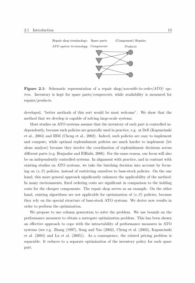
tiple spare parts are required to repair a component. For a summary of the different
terminologies, we refer to Figure 2.1. Our research is not restricted to application in
repair shops, but is also applicable to general ATO systems.
Song and Zipkin (2003) give an extensive review and motivation of the study of ATO
systems. They find that “many real ATO systems contain hundreds of components and
thousands of products”. The system that we consider is an example of such a large-
scale system. While some methods capable of working with large-scale systems have been
2.1 Introduction 13
Repair shop terminology:
ATO system terminology:
Spare parts
Components
(Component) Repairs
Products
Figure 2.1: Schematic representation of a repair shop/assemble-to-order(ATO) sys-
tem. Inventory is kept for spare parts/components, while availability is measured for
repairs/products.
developed, “better methods of this sort would be most welcome”. We show that the
method that we develop is capable of solving large-scale systems.
Most studies on ATO systems assume that the inventory of each part is controlled in-
dependently, because such policies are generally used in practice, e.g. at Dell (Kapuscinski
et al., 2004) and IBM (Cheng et al., 2002). Indeed, such policies are easy to implement
and compute, while optimal replenishment policies are much harder to implement (let
alone analyze) because they involve the coordination of replenishment decisions across
different parts (e.g. Benjaafar and ElHafsi, 2006). For the same reason, our focus will also
be on independently controlled systems. In alignment with practice, and in contrast with
existing studies on ATO systems, we take the batching decision into account by focus-
ing on (s, S) policies, instead of restricting ourselves to base-stock policies. On the one
hand, this more general approach significantly enhances the applicability of the method:
In many environments, fixed ordering costs are significant in comparison to the holding
costs for the cheaper components. The repair shop serves as an example. On the other
hand, existing algorithms are not applicable for optimization of (s, S) policies, because
they rely on the special structure of base-stock ATO systems. We derive new results in
order to perform the optimization.
We propose to use column generation to solve the problem. We use bounds on the
performance measures to obtain a surrogate optimization problem. This has been shown
an effective approach to cope with the intractability of performance measures in ATO
systems (see e.g. Zhang (1997), Song and Yao (2002), Cheng et al. (2002), Kapuscinski
et al. (2004) and Lu et al. (2005)). As a consequence, the related pricing problem is
separable: It reduces to a separate optimization of the inventory policy for each spare
part.
14 Spare parts inventory control for an aircraft component repair shop
To perform this optimization efficiently, we develop a novel algorithm. The algorithm
is based on a grid of parallelograms that together cover the policy space. We derive a
lower bound for the costs of policies enclosed in such a parallelogram, which is utilized
to determine which areas of the grid need refinement. The lower bound is based on a
generic decomposition of the costs in an increasing and a decreasing part. Therefore, the
algorithm works under more general conditions than existing algorithms. For example,
unlike existing exact algorithms, it can handle fill rate type of constraints.
This approach, including the column generation algorithm, was implemented in a
decision support system (DSS). This system is now used on a daily basis at the repair
shop owned by Fokker Services.
In summary, the contributions of the chapter are as follows. We develop an algorithm
to determine cost-efficient inventory control policies for ATO systems. Unlike existing
algorithms, the algorithm is capable of handling the large-scale systems that are prevalent
in practice. We demonstrate this in a computational study. Moreover, the algorithm is
the first to consider optimization of (s, S) policies in an ATO system, which is a significant
improvement on base-stock policy optimization in terms of applicability. We give evidence
that implementing the method at a repair shop improves inventory control. In addition, we
contribute by proposing a novel, more generally applicable algorithm to solve the pricing
problem. Because the pricing problem is equivalent to single-item policy optimization,
this algorithm is a contribution in its own right, outside of the framework presented here.
The remainder of this chapter is organized as follows. In the next section, the literature
on ATO systems is reviewed. In Section 2.3 we formulate the optimization problem.
In Section 2.4, we describe the optimization algorithm and in Section 2.5, we present
a computational study to evaluate the performance of the algorithm. In Section 2.6,
we report on the implementation of the method at the repair shop. We conclude in
Section 2.7.
2.2 Literature review
In this section, we adopt the terminology used in existing studies of ATO systems (see
Figure 2.1).
The optimization and evaluation of ATO systems is generally performed under heuris-
tic policy types, as such policies are often used in practice because they are easy to
implement. (Also, the structure of the optimal policy is unknown in the general case; e.g.
Benjaafar and ElHafsi (2006) and Dogru et al. (2010) derive the optimal policy structure
for special cases.) In particular, most studies focus on independent base-stock policies.
2.2 Literature review 15
These studies can be characterized into continuous review models and periodic review
models. We will now give an overview of the main results.
We first discuss continuous review models. In general, these studies assume Poisson
demand for products, while integer numbers of components are used in a single prod-
uct. Song and Yao (2002) consider a single product system under independent identically
distributed (iid) component leadtimes. They minimize the number of back-orders un-
der a budget constraint, by using bounds on the number of back-orders as a surrogate
objective function. Algorithms are developed to solve this problem. Along the same
lines, algorithms are proposed to minimize the inventory costs under a surrogate fill rate
constraint. The multi-product extension is studied by Lu et al. (2005). They consider
budget-constrained back-order minimization, where again bounds on the expected num-
ber of back-orders are used as a surrogate objective function. The resulting problem has a
stack structure. As a result, the problem can be solved by solving k! subproblems greedily,
where k denotes the number of products. Lu and Song (2005) consider order-based cost
minimization for the same system, under the assumption that each product uses either 1,
or 0 components. Back-order costs are paid per product back-ordered per time unit. They
derive various properties of the cost function, based on which an optimization approach is
formulated. The optimization algorithm evaluates the costs of m7 logm solutions, where
m is the number of components. Gullu and Koksalan (2012) consider a system similar
to ATO systems, but with a different resupply system. Components that are withdrawn
together are replenished together (except for one component in each demand, which is
replenished via a separate channel). Exact expressions are derived for the performance
of the system. However, evaluation of these expressions is not tractable for large-scale
systems. The authors propose a greedy heuristic to optimize the base-stock levels.
We conclude that existing algorithms for the optimization in the continuous review
setting are either only applicable to single-product systems, or can only be used for
relatively small instances. None of the proposed algorithms is capable of solving the
instances that we consider.
Other studies in the continuous review setting mainly consider the evaluation of key
performance measures such as fill rates and average back-orders in base-stock ATO sys-
tems. As exact evaluation is generally intractable for large systems, many contributions
derive bounds on and approximations of performance characteristics. In the following, we
briefly discuss such contributions. For deterministic leadime systems, Song (1998) focuses
on the fill rate and Song (2002) studies the average number of product back-orders. Lu
et al. (2003) extend Song (1998) to iid leadtimes. Cheung and Hausman (1995) show
how to evaluate the average number of customer back-orders for a system with iid lead-
16 Spare parts inventory control for an aircraft component repair shop
times, under the assumption of complete cannibalization. In the make-to-stock setting,
Glasserman and Wang (1998) show that there is a linear relationship between delivery
time and inventory, in the limit of high fill rates. In the same setting, Song et al. (1999)
develop methods for exact fill rate evaluation, and Dayanik et al. (2003) compare different
bounds on the fill rate. Batching policies, in particular (R, nQ) policies, are considered
by Song (2000) and Zhao and Simchi-Levi (2006). Song (2000) finds that the analysis of
such policies reduces to the analysis of base-stock ATO systems, under general conditions.
However, as Zhao and Simchi-Levi (2006) point out, the evaluation of a single (R, nQ)
policy in this way requires the evaluation of a number of base-stock ATO systems that
is exponential in the number of components. To cope with this difficulty, they propose
sampling procedures to efficiently simulate batching policies.
We now give an overview of periodic review systems. For such systems, demand is
generally assumed to be multivariate normal. This assumption is reasonable for some high-
volume systems. It is unsuitable when the discrete nature of inventory cannot be ignored,
e.g. inventories of components for higher-end low-volume products, and inventories for
spare parts. In particular, approaches that depart from this assumption are inapplicable
for the problem we consider. Periodic review studies generally assume base-stock control
for components, deterministic leadtimes and a first come, first serve (FCFS) component
allocation policy, but differ in the policy by which components are allocated to demands
that arrived in the same period.
Hausman et al. (1998) develop a heuristic which uses an equal fill rate for each compo-
nent. The approach is limited in its use because it cannot properly account for different
fill rate targets for different products. Zhang (1997) assumes fixed priority allocation, and
considers cost minimization with product-specific fill rate restrictions. It is shown that
the feasible region for the problem is convex, and an optimal solution is determined by
employing a feasible direction algorithm. Agrawal and Cohen (2001) find similar results
under a fair share allocation rule. Cheng et al. (2002) study a PC assembly system for
which they minimize the costs under a product-specific fill rate constraint. Special pur-
pose algorithms are developed, based on a lower bound on the fill rate. The proposed
algorithm is only applicable under the assumption that each product uses a unique com-
ponent. Because demand is continuous, it can then be shown that all constraints are
binding. The algorithm is tested for a 18 product, 17 component system, but computa-
tion times are not reported. For the general case a greedy heuristic is proposed, which
remains untested. Akcay and Xu (2004) consider weighted time-window fill rate maxi-
mization under a budget constraint. Unlike the studies discussed earlier, the allocation
rule in their approach is dynamic. Moreover, their analysis is not restricted to a specific
2.3 The optimization problem 17
demand distribution. The problem is modeled as a two-stage stochastic program. A sam-
ple average approximation is employed to find a solution. Unfortunately, this algorithm
is not scalable to larger instances, because the number of scenarios required to decently
represent the stochastic behavior increases for larger systems. Solving the integer problem
associated with a sample quickly becomes intractable when the number of scenarios in
the sample increases.
We propose an algorithm based on column generation. This study is the first to
propose such an approach in an ATO setting. The approach has been used for multi-
item inventory optimization problems by a number of authors. E.g. Kranenburg and Van
Houtum (2007b) use it to investigate commonality in a single-location model, Kranenburg
and Van Houtum (2008) employ the approach in a single-location system with multiple
demand classes, Wong et al. (2007) use it in a multi-echelon system, and Kranenburg and
Van Houtum (2009) use it for optimization of base-stock policies in a single-echelon multi-
location inventory system with partial pooling. Topan et al. (2010) develop techniques
to use the approach in a multi-echelon system with (r,Q) policies instead of base-stock
policies in the central warehouse.
2.3 The optimization problem
In this section, we formulate the optimization problem and the model underlying it.
The model is described in Section 2.3.1. In Section 2.3.2, we derive bounds on perfor-
mance measures that are used to formulate the optimization model, which is given in
Section 2.3.3. In Section 2.3.4 we discuss the pricing problem associated with our opti-
mization problem. We use repair shop terminology in the remainder of the chapter (see
Figure 2.1).
2.3.1 The model
We consider a repair shop where various types of components are repaired. Components
needing repair arrive according to a Poisson process. Upon arrival of a defect component,
inspection reveals which spare parts are needed to repair it.
Spare parts are stocked in a local warehouse. Inventory is under continuous review,
and is controlled using independent (s, S) policies. Under an (s, S) policy, when the
inventory position (= inventory on hand + inventory on order − backlogs) is at or below
s, an order is placed to raise it to S. As discussed in Section 2.1, controlling inventory
independently is attractive from a practical point of view. We focus on (s, S) policies
18 Spare parts inventory control for an aircraft component repair shop
because they allow the company to both control fixed ordering costs and to hedge against
stock-out risk by keeping a safety stock. Moreover, the (s, S) policy is easy to grasp for
practitioners, making it a commonly applied inventory control policy. Indeed, this policy
is used by the repair shop at which this research was performed. Because delaying the
placement of a replenishment order for a part with backlogs is not common in practice,
we assume s ≥ −1.We assume stochastic sequential leadtimes. Svoronos and Zipkin (1991) give a precise
definition of such leadtimes, and argue that this may be a more realistic assumption than
iid leadtimes. We assume that the supplier delivers the orders in full. The leadtime
distribution may be different for different parts. We make no restrictive assumptions
regarding the leadtime distribution.
We assume that unmet demands for spare parts are fully back-ordered. This matches
the real-life case at the repair shop. However, the consequences of spare parts shortages
may be mitigated at the repair shop by informing the supplier about the shortage, in an
attempt to expedite existing orders for the spare parts. However, making such interven-
tions part of the inventory model is difficult because of missing data, and may not even
be desirable because it may make the outcomes of the inventory model more difficult to
interpret for practitioners.
Spare parts are allocated to repairs on a FCFS basis. This allocation policy is com-
monly used in ATO practice and literature (for exceptions see e.g. Lu et al. (2010), Dogru
et al. (2010), and references therein), and it matches the policy that is used at the repair
shop. When some parts for a repair are available but others are not, the available parts
are put aside as committed inventory (see e.g. Song (2002) and Zhao and Simchi-Levi
(2006)).
We denote the set of spare parts by J . The component repair types are denoted by
I. We introduce the following notation:
• hj > 0: inventory holding costs per unit of time per unit of inventory of part j ∈ J .
• oj ≥ 0: the fixed ordering costs for a single order for parts j ∈ J .
• Cj: the set of policies for part j ∈ J . For each valid combination of s and S, we
have (s, S) = c ∈ Cj.
• Ij ⊂ I: set of repair types in which part j may be used. We allow Ij = I, but inpractice, parts are only used in a limited range of repair types.
• J i ⊂ J : set of parts that may be used in a repair of type i.
2.3 The optimization problem 19
• Y i(n) = (Y ij (n), j ∈ J i): random vector indicating the spare parts needed in the
nth repair of type i ∈ I. We assume that Y ij (n) ∈ {0, 1, 2, . . .} and that Y i(n) for
n ∈ {1, 2, . . .} are iid random variables. We allow for dependence between Y ij (n) for
different parts j.
• λi: the Poisson arrival rate of repairs of type i.
• ti(n): (random) time of arrival of the nth repair of type i ∈ I.
• λj =∑
i∈Ij λiP(Y i
j (1) > 0): the rate at which repairs arrive that require part j.
Also: the demand rate for part j (note that demand for part j is compound Poisson).
• I(t−) = (Ij(t−, cj), j ∈ J ): (random) inventory on hand just before time t. The
dependence of Ij on the policies cj ∈ Cj will be dropped where no confusion can
arise.
• P (t) = (Pj(t, cj), j ∈ J ): (random) number of purchase orders in the time period
(0, t).
• W i(n): (random) waiting time until all spare parts needed in the nth repair of
type i are available. W i denotes the random waiting time for an arbitrary repair as
n→∞.
2.3.2 Bounds on performance measures
Repairs of a given type may typically require a broad range (10-50) of spare parts, each
with low probability. As a result of the dependence between the inventory level of differ-
ent parts, exact evaluation of the time-window fill rate P(W i < w) or expected waiting
time E(W i) for such repair types is intractable (see Song (1998) and Song (2002), respec-
tively). A well-established method to cope with this difficulty is the use of bounds on
the performance measures. We will now derive bounds on the performance of (s, S) ATO
systems, such as the repair shop we consider.
We first derive a bound on the fill rate. We concentrate on bounds on the immediate
fill rate, because the time-window fill rate corresponds to the immediate fill rate in a
system with revised leadtimes. (For details see Proposition 1.1 of Song (1998), which
extends with little difficulty to stochastic sequential leadtimes.) For the nth repair of
type i, P(Ij(ti(n)−) < Y i
j (n)) equals the probability that the waiting time for parts of
20 Spare parts inventory control for an aircraft component repair shop
type j is positive. We thus have
P(W i(n) = 0) = 1−P
⎛⎝⋃
j∈J i
Ij(ti(n)−) < Y i
j (n)
⎞⎠ (2.1)
≥ 1−∑j∈J i
P(Ij(t
i(n)−) < Y ij (n)), (2.2)
where the inequality is typically referred to as Boole’s inequality. By taking the limit
n→∞, we obtain a bound on the long-term fill rate. Note that this bound is tight if the
waiting time of repairs is always caused by an inventory shortage of a single spare part
only.
For the expected waiting time, we have:
E(W i) =
∫ ∞w=0
(1−P(W i ≤ w))dw. (2.3)
We bound this integral by a Riemann sum: Let 0 = w1 < w2 < . . . < wM be an arbitrary
sequence such that P(W i ≤ wM) = 1. Then
E(W i) ≤M∑
m=2
(wm − wm−1)(1−P(W i ≤ wm−1)). (2.4)
The bound in (2.2) can subsequently be used in the summand, to obtain an efficiently
computable lower bound on the average waiting time.
We now briefly discuss (R, nQ) policies, which are also common in practice. Since we
consider non-unit demand, such policies are different from (s, S) policies (see e.g. Axsater
(2006, pp. 48-49)). While the bound (2.2) remains valid for (R, nQ) policies, it can
be strengthened when the inventory position has uniform equilibrium distribution (see
Song (2000) for conditions). If in addition for given i ∈ I and n the random variables
Y ij (n), j ∈ J i are associated (e.g. independent), then Y i
j (n) − Ij(ti(n)), j ∈ J i are also
associated, in the limit n → ∞. The proof is along the same lines of the proof of
Proposition 5.1 of Song (1998). We omit details. As a result, the following bound holds:
P(W i = 0) ≥∏j∈J i
limn→∞
P(Ij(ti(n)) ≥ Y i
j (n)). (2.5)
A surrogate constraint based on this bound can be linearized by taking the logarithm on
both sides (cf. Song and Yao (2002)). Note that (2.5) is not a valid bound for (s, S)
policies. The algorithm that we develop in Section 2.4 can be applied to (R, nQ) policies
2.3 The optimization problem 21
with minor modifications. Let Cj be the set of (R, nQ) policies for part j, and use the
correspondence R↔ s, R +Q↔ S when solving the pricing problem.
2.3.3 Cost minimization under fill rate constraints
This chapter is focused on cost minimization under repair type specific fill rate constraints.
Based on the bounds derived in the previous section, the approach we propose can be
extended to include constraints on the average waiting time, on the time-window fill rate,
or combinations of such constraints. The focus on the immediate fill rate is thus mainly for
simplicity of notation and exposition. In addition, the fill rate is a performance measure
which is easily communicated with managers and customers. The formulation on which
we focus is thus easily applicable in practice.
A natural formulation of the problem would use the policies (s, S) = c ∈ Cj directly as
decision variables. However, such a formulation would be non-linear, and even non-convex,
which would render it computationally intractable. Instead, we propose to let xjc = 1
indicate that policy c = (s, S) is used for part j, while xjc = 0 indicates that policy c is not
used for part j. This will linearize the optimization problem, at the cost of introducing
an infinite number of decision variables since Cj is infinite. This difficulty, in contrast
with the difficulties associated with a non-convex model, turns out to be manageable
using the techniques developed in the next section: The algorithm we will develop needs
to consider only a small number of decision variables xjc explicitly to conclude that the
current solution is close-to-optimal. The linearization leads to the following optimization
problem:
min∑j∈J
∑c∈Cj
xjc(Hj(c) +Oj(c)), (2.6)
s.t.∑j∈J i
∑c∈Cj
xjcFij (c) ≤ 1− ai, i ∈ I, (2.7)
∑c∈Cj
xjc = 1, j ∈ J , (2.8)
xjc ∈ {0, 1}, j ∈ J , c ∈ Cj. (2.9)
22 Spare parts inventory control for an aircraft component repair shop
Here, ai denotes the target fill rate for repairs of type i, and
Hj(c) = Hj(s, S) = limt→∞
hjE (Ij(t, c)) , (2.10)
Oj(c) = Oj(S − s) = limt→∞
ojE (Pj(t, c)/t) , (2.11)
F ij (c) = F i
j (s, S) = limn→∞
P(Ij(t
i(n)−, c) < Y ij (n)). (2.12)
In particular, for part j ∈ J , Hj denotes the holding costs and Oj the ordering costs. F ij
is the probability that the inventory for part j is insufficient to cover the demand of an
arbitrary repair of type i.
The bound in (2.2) is used in this formulation to guarantee that the fill-rate constraints
are satisfied. Note that this guarantee applies regardless of any correlation between the
demand probabilities Y ij (n), j ∈ J i; which is important since such correlations are hard
to estimate in practice. Approaches along these lines have been used in ATO literature
(Zhang, 1997; Song and Yao, 2002), and by a number of companies (e.g. IBM (Cheng
et al., 2002) and Dell (Kapuscinski et al., 2004)).
We now discuss the evaluation of (2.10-2.12). For k ∈ {0, . . . , S − s− 1}, mk denotes
the probability to visit inventory position S − k during an arbitrary order cycle. mk can
be evaluated recursively using the compounding distribution of demand for part j, see e.g.
Axsater (2006, pp. 107-109). The expected length of an order cycle is given by MS−s/λj,
with MS−s =∑S−s−1
k=0 mk. The holding costs for general policies can be expressed in terms
of the holding costs for (S − 1, S) policies as follows:
Hj(s, S) =1
MS−s
S−s−1∑k=0
mkHk(S − k − 1, S − k). (2.13)
The same expression holds with F ij and F i
k replacing Hj and Hk, respectively. Since a
single order is placed in each order cycle, we have Oj(S − s) = ojλj/MS−s.
To solve the optimization problem (2.6-2.9), we will use the solution of the associated
continuous relaxation, which is obtained by replacing (2.9) by
0 ≤ xjc ≤ 1 j ∈ J , c ∈ Cj. (2.14)
To strengthen the lower bound that is obtained via this relaxation, we note that for any
policy c for a part j that does not satisfy
F ij (c) ≤ 1− ai, i ∈ Ij, (2.15)
2.3 The optimization problem 23
the decision variable xjc must take the value 0 in any feasible solution to (2.6-2.9). From
now on, policies which do not satisfy (2.15) are no longer considered to be included in Cj.While excluding these policies does not change the optimal solution of (2.6-2.9), it does
increase the objective value of (2.6-2.8,2.14), and thus improves the quality of the lower
bound.
2.3.4 The pricing problem
In this section, we first investigate the problem of finding the column xjc with the lowest
reduced costs for given dual multipliers. We then briefly discuss the equivalence of this
problem with a single-item inventory problem. The reduced cost associated with decision
variable xjc is given by
Rj(c) = Rj(s, S) = Hj(s, S) +Oj(s, S) + μj +∑i∈Ij
νiF ij (s, S), (2.16)
where νi ≥ 0, i ∈ I are the dual multipliers associated with (2.7), and μj is a dual
multiplier associated with (2.8).
To determine whether any decision variables exist with negative reduced costs, we
determine for each part j the solution of
min−1≤s<S
Rj(s, S) such that F ij (s, S) ≤ 1− ai, i ∈ Ij, (2.17)
where the constraints result from our restriction of Cj to policies satisfying (2.15).
To show that finding decision variables with negative reduced cost is equivalent to
minimizing the costs for a single-item inventory model, we define
G(y) = Hj(y − 1, y) +∑i∈Ij
νiF ij (y − 1, y) + μj. (2.18)
We now rewrite (2.16) as
Rj(s, S) = Oj(S − s) +M−1S−s
S−s−1∑k=0
mkG(S − k). (2.19)
This formulation is similar to many single-item formulations, e.g. Zheng and Federgruen
(1991).
However, G(·) need not be quasiconvex as a consequence of the fact that F ij corresponds
to the component-specific part fill rate. This renders many algorithms, in particular the

24 Spare parts inventory control for an aircraft component repair shop
one proposed by Zheng and Federgruen (1991), inapplicable. In addition, (2.17) features
fill rate type of constraints, which cannot be accounted for in existing algorithms, in
particular the algorithm proposed by Chen and Feng (2006). In Section 2.4.2, we propose
a new, efficient and exact algorithm for (2.17).
The algorithm is interesting in its own right as a solution method for single-item
problems, because it works under very general conditions. In particular, G(·) need not be
quasiconvex, but only decomposable into an increasing and a decreasing function, a much
weaker condition. In addition, we can allow for constraints on the average waiting time,
the fill rate, or any other service measure F (s, S) for which F (S − 1, S) is nonincreasing
in S. We are not aware of existing methods that can efficiently compute the optimal (s, S)
policy for single-item problems under these conditions.
2.4 The algorithm
The algorithm to solve (2.6-2.9) consists of two steps: We first solve the continuous
relaxation (2.6-2.8,2.14) to obtain a lower bound, and we then apply a procedure to
find an integer solution. We use a column generation approach to solve the continuous
relaxation. We describe this column generation approach in Section 2.4.1. In Section 2.4.2
we describe the algorithm to solve the pricing problem. Finally, we develop methods to
find integer solutions in Section 2.4.3.
2.4.1 Column generation algorithm
Our column generation approach to solve the continuous relaxation can be summarized
as follows:
Algorithm 2.1
Step 1: Initialization Determine an initial set of policies C ′j ⊂ Cj for each part j, by
executing the initialization step of Algorithm 2.2.
Step 2: Master Problem Solve the restricted master problem (2.6-2.8,2.14) with Cjreplaced by C ′j. This gives us a primal and dual solution.
Step 3: Pricing Problem For the dual multipliers obtained in Step 2, execute for each
part j Steps 1-3 of Algorithm 2.2. This adds the policy c ∈ Cj with the lowest reduced
cost to C ′j, typically along with other policies that also have low reduced costs.

2.4 The algorithm 25
s
S
c′′ = (s′′, S ′′)
c′ = (s′, S ′)
Figure 2.2: The parallelogram spanned by the policies c′ and c′′. Policies covered by the
parallelogram are circled.
Step 4 If any policies with negative reduced costs were added to C ′j for any part j in the
previous step, go to Step 2. Otherwise, terminate.
When this algorithm terminates, we obtain the optimal solution to (2.6-2.8,2.14). The
solution value is a lower bound on the solution value of the integer problem (2.6-2.9).
2.4.2 Algorithm for the pricing problem
To solve the pricing problem in Step 3 of Algorithm 2.1, we develop an algorithm to solve
(2.17) for given dual multipliers νi and μj. Throughout this section, we will suppress
subscript j (in particular, I will denote Ij). The algorithm is based upon the following
key observation.
Proposition 2.1 Let two policies c′ = (s′, S ′) and c′′ = (s′′, S ′′) with S ′ − s′ ≥ S ′′ − s′′
and S ′′ ≥ S ′ be given. Consider all policies covered by the parallelogram spanned by the
policies (s′, S ′) and (s′′, S ′′) in the (s, S) plane (circled in Figure 2.2). The reduced costs
for these policies, as given by (2.16), are bounded below by
R(c′, c′′) = H(s′, S ′) +O(S ′ − s′) +∑i∈I
νiF i(s′′, S ′′) + μ. (2.20)
In addition, if c′′ violates (2.15), then all policies inside the parallelogram do.
For proofs, we refer to the appendix to this chapter.
The algorithm we propose is based on a grid of parallelograms, each of the type
described in Proposition 2.1. We denote such a parallelogram by g = (c′(g), c′′(g)) =
(s′, S ′; s′′, S ′′), with c′(g) and c′′(g) the policy in the lower left and upper right corner of
g, respectively (see Figure 2.2). For a collection of parallelograms G, we define C(G) as

26 Spare parts inventory control for an aircraft component repair shop
{c′(g)|g ∈ G} ∪ {c′′(g)|g ∈ G}. Note that C(G) may contain policies that violate (2.15),
and therefore C(G) ⊂ C.We now sketch the general idea behind the algorithm for the pricing problem. Details
will be given later.
Algorithm 2.2
Initialization Construct a grid of parallelograms G, such that each relevant policy (s, S)
is covered by at least one parallelogram g ∈ G. Initialize the set of policies C ′ =C(G) ∩ C. Thus, only policies in the corners of each parallelogram are initially
considered.
Step 1 Select c∗ ∈ argminc∈C′ R(c), where R(c) is given by (2.16).
Step 2 For any g ∈ G for which R(c′(g), c′′(g)) < R(c∗) and for which c′′(g) satisfies
(2.15)
Refine parallelogram: There might be policies c covered by g (but c /∈ C ′) that
improve on c∗ and satisfy (2.15). Remove g from G, and add to G a number of
smaller parallelograms that together cover all policies originally covered by g.
Note that by Proposition 2.1: 1) if R(c′(g), c′′(g)) ≥ R(c∗), then policies covered by
g cannot improve on c∗ and 2) if c′′(g) violates (2.15), then all covered policies do.
In both cases, covered policies need not be evaluated.
Step 3 If any parallelogram was refined in Step 2, update C ′ = C(G) ∩ C and go to Step
1. Otherwise, terminate returning c∗. G is stored for future calls to Steps 1-3.
This algorithm terminates, as parallelograms that need refining will become smaller and
smaller until they cover only a single policy. In Section 2.5, we show that the algorithm
only evaluates a small number of policies.
In the remainder of this section, we will describe each step in detail. We determine a
finite set of policies that contains the policy with lowest reduced costs. We also describe
how to ensure computational efficiency. Next, we examine the construction of the grid
in more detail and finally we discuss how to replace a parallelogram by smaller parallelo-
grams.
Determining relevant policies
To determine a finite set that contains the policy (s∗, S∗) with lowest reduced costs, we
determine ξ such that s∗ + S∗ < ξ. To find such an upper bound ξ, we will use the
following proposition:

2.4 The algorithm 27
Proposition 2.2 For every policy (s, S)
Hj(s, S) ≥ Hj
(s+ 1 + S
2− 1,
s+ 1 + S
2
), (2.21)
where Hj(y − 1/2, y + 1/2) for integer y is defined as the average of Hj(y − 1, y) and
Hj(y, y + 1).
For the proof we refer to the appendix to this chapter. Now, define
y(u) = min
(y′|H(y′ + 1
2− 1,
y′ + 1
2
)> u
). (2.22)
Let u be an upper bound on R(s∗, S∗)− μ. Then, for any (s, S) such that s+ S ≥ y(u),
R(s, S) ≥ H(s, S) + μ ≥ H
(s+ 1 + S
2− 1,
s+ 1 + S
2
)+ μ > u+ μ ≥ R(s∗, S∗),
(2.23)
where the second inequality follows from Proposition 2.2.
When Algorithm 2.2 is used in a stand-alone manner to solve single-item inventory
problems, we can thus set ξ = y (R(c)− μ) for any policy c. When Algorithm 2.2 is
initialized as part of the Initialization step of Algorithm 2.1, no values of νi are available. It
is then impossible to find an upper bound on R(s∗, S∗)−μ. To proceed, determine a policy
c such that F i(c) is negligibly small for all i ∈ I. Set u = R(c)−μ−∑i∈I Fi(c)νi = H(c)+
O(c), and use ξ = y(u). After execution of Algorithm 2.2, check whether R(c∗)− μ ≤ u,
which indicates that u was a valid bound.
If the bound turns out to be invalid, determine a new value for ξ based on R(c∗)− μ.
Expand the grid to cover the added policies, and continue at Step 2 of Algorithm 2.2.
Because the new bound is guaranteed to be valid, the algorithm will then terminate at the
optimum. However, in our experiments, such a second run was never needed to guarantee
optimality.
Ensuring computational efficiency
For each policy (s, S) that is added to C(G), we determine H(s, S)MS−s and F i(s, S)MS−sfor i ∈ I, using
H(s− 1, S)MS−s+1 = H(s, S)MS−s +H(s− 1, s)mS−s, (2.24)
28 Spare parts inventory control for an aircraft component repair shop
and similar for F i. So for each (s, S) that is added to C(G), we first determine whether
any policies (s′, S) with s′ > s are already evaluated. In that case, H(s, S)MS−s is calcu-
lated from H(s′, S)MS−s′ by repeated use of (2.24), and similar for F i(s, S)MS−s′ . The
computational effort of executing the algorithms thus depends critically on the number
of values for S for which policies (s, S) need to be evaluated.
Grid construction
Several methods for constructing a covering grid during initialization of Algorithm 2.2
have been tested. We find that the algorithm is efficient regardless of the precise method
that is used, as long as two conditions are satisfied. First, the grid should be sufficiently
sparse. Also, there should be only a small number of values for S for which any policies
are initially added to c ∈ C ′.We describe a method that we have found to have particularly robust performance
across all parts. Determine first the values that will be used for S and Δ = S−s > 0 in C ′.Take {S1, S2, . . . , SN} = {0, 1, 2, 3, 4, 6, 8, 12, 16, . . . , ξ} (the step-size Sn+1 − Sn doubles
whenever a power of two above 2 is reached). Use a similar range for {Δ1,Δ2, . . . ,ΔM},but starting at 1.
Now let
G = {(g = (Sn −Δm+1, Sn;Sn+1 −Δm, Sn+1)|n ∈ {0, N − 1},m ∈ {0,M − 1}}. (2.25)
We then let G consist of all parallelograms g ∈ G that cover at least some policies (s, S)
such that −1 ≤ s < S and s+S < ξ. Figure 2.3 depicts parallelograms g ∈ G constructed
in this manner, for the lower left area of the policy space that needs to be covered.
Refining a parallelogram
When a parallelogram g = (s′, S ′; s′′, S ′′) needs to be refined in Step 2 of Algorithm 2.4.2,
it is replaced by a number of smaller parallelograms covering the same policies. We
consider two cases, see Figure 2.4:
• S ′ − s′ = S ′′ − s′. We replace the parallelogram by a number of parallelograms for
which S ′ − s′ = S ′′ − s′
• S ′ − s′ = S ′′ − s′. The parallelogram is split into two parallelograms of equal size.
The reason for refining in this manner is that it limits the number of values for S for
which policies need to be evaluated.
2.4 The algorithm 29
-1 3110
512
s
S
Figure 2.3: Some parallelograms g ∈ G after initial construction.
S ′ − s′ = S ′′ − s′′
(s′′, S ′′)
(s′, S ′)
(s′′, S ′′)
(s′, S ′)
S ′ − s′ = S ′′ − s′′
Figure 2.4: Refining a parallelogram g = (s′, S ′; s′′, S ′′). Two cases are distinguished.
2.4.3 Finding integer solutions
In Section 2.4.1, we developed a method to solve the continuous relaxation (2.6-2.8,2.14).
We will now present two algorithms to obtain feasible solutions for the discrete problem.
Both algorithms are based on Algorithm 2.1 and iteratively fix policies for a subset of
parts.
The first algorithm applies sequential rounding. Intuitively, it fixes the policy for one
part at a time, each time selecting the policy with the highest primal value. Parts that
are more discrete are fixed first. We have found hj to be a good measure of discreteness.
30 Spare parts inventory control for an aircraft component repair shop
The actual algorithm is slightly more complicated, because we have to prevent rounding
to infeasible policies:
Algorithm 2.3
Initialization Initialize the set J of parts for which a policy still needs to be fixed as J .Initialize the fill rate targets ai as ai.
Step 1 Solve the continuous relaxation, with the parts restricted to J . Use 1− ai as the
RHS in (2.7) and (2.15) to account for the policies that are already fixed.
Step 2 Select the part j ∈ J with highest hj. Select c∗ ∈ argmax{xjc : c ∈ C ′j} and fix
that policy for part j. Update ai ← ai + F ij (c
∗), and remove j from J .
Step 3 If J = ∅, terminate. Otherwise, go to Step 1.
Recall that we applied column generation to solve the continuous relaxation (2.6-
2.8,2.14). A common approach to find a feasible solution in such a situation is to consider
the mixed integer program containing only the columns that have been generated when
solving the continuous relaxation. However, for larger instances, the number of binary
variables in these integer problems becomes too large. The second algorithm therefore
divides the set of spare parts J into a set Jdisc of discrete spare parts for which a single
policy must be selected and a set Jcont for which we allow a mixture of policies. The
size of the set Jdisc determines the difficulty of solving the mixed integer problem with
branch-and-bound. This size is controlled by a parameter K0. This gives rise to the
following algorithm.
Algorithm 2.4
Initialization Initialize the set of parts for which a policy still needs to be fixed J as J .Initialize the fill rate targets as ai = ai. Set K = K0.
Step 1 Define Jdisc as the K parts in J that have highest values hj. Set Jcont = J \Jdisc.
Solve this mixed integer problem by branch-and-bound. Use 1 − ai as the RHS in
(2.7) and (2.15) to account for the policies that are already fixed.
Step 2 Fix for all parts j ∈ Jdisc the policy j that is selected in the solution from the
previous step. Update the values ai and remove Jdisc from J . Set K = 32K.
Step 3 If J = ∅, terminate. Otherwise, go to Step 1.
The computation time to solve the mixed integer program by branch-and-bound can be
decreased by providing it with a starting solution. We apply Algorithm 2.3 to the parts
in J to obtain such a starting solution.
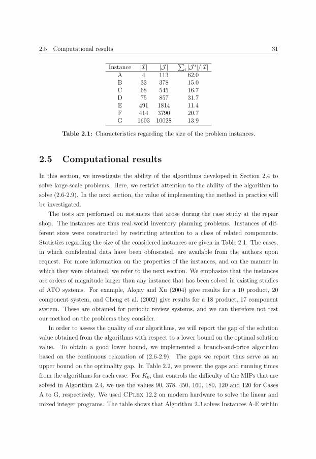
2.5 Computational results 31
Instance |I| |J | ∑i |J i|/|I|A 4 113 62.0B 33 378 15.0C 68 545 16.7D 75 857 31.7E 491 1814 11.4F 414 3790 20.7G 1603 10028 13.9
Table 2.1: Characteristics regarding the size of the problem instances.
2.5 Computational results
In this section, we investigate the ability of the algorithms developed in Section 2.4 to
solve large-scale problems. Here, we restrict attention to the ability of the algorithm to
solve (2.6-2.9). In the next section, the value of implementing the method in practice will
be investigated.
The tests are performed on instances that arose during the case study at the repair
shop. The instances are thus real-world inventory planning problems. Instances of dif-
ferent sizes were constructed by restricting attention to a class of related components.
Statistics regarding the size of the considered instances are given in Table 2.1. The cases,
in which confidential data have been obfuscated, are available from the authors upon
request. For more information on the properties of the instances, and on the manner in
which they were obtained, we refer to the next section. We emphasize that the instances
are orders of magnitude larger than any instance that has been solved in existing studies
of ATO systems. For example, Akcay and Xu (2004) give results for a 10 product, 20
component system, and Cheng et al. (2002) give results for a 18 product, 17 component
system. These are obtained for periodic review systems, and we can therefore not test
our method on the problems they consider.
In order to assess the quality of our algorithms, we will report the gap of the solution
value obtained from the algorithms with respect to a lower bound on the optimal solution
value. To obtain a good lower bound, we implemented a branch-and-price algorithm
based on the continuous relaxation of (2.6-2.9). The gaps we report thus serve as an
upper bound on the optimality gap. In Table 2.2, we present the gaps and running times
from the algorithms for each case. For K0, that controls the difficulty of the MIPs that are
solved in Algorithm 2.4, we use the values 90, 378, 450, 160, 180, 120 and 120 for Cases
A to G, respectively. We used CPlex 12.2 on modern hardware to solve the linear and
mixed integer programs. The table shows that Algorithm 2.3 solves Instances A-E within
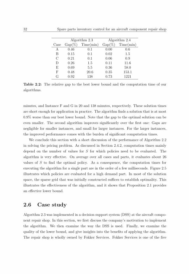
32 Spare parts inventory control for an aircraft component repair shop
Algorithm 2.3 Algorithm 2.4Case Gap(%) Time(min) Gap(%) Time(min)A 0.46 0.1 0.00 0.6B 0.15 0.1 0.02 1.5C 0.21 0.1 0.06 0.9D 0.26 1.5 0.11 11.6E 0.69 5.5 0.36 58.0F 0.48 20.6 0.35 153.1G 0.92 138 0.73 1221
Table 2.2: The relative gap to the best lower bound and the computation time of our
algorithms.
minutes, and Instance F and G in 20 and 138 minutes, respectively. These solution times
are short enough for application in practice. The algorithm finds a solution that is at most
0.9% worse than our best lower bound. Note that the gap to the optimal solution can be
even smaller. The second algorithm improves significantly over the first one: Gaps are
negligible for smaller instances, and small for larger instances. For the larger instances,
the improved performance comes with the burden of significant computation times.
We conclude this section with a short discussion of the performance of Algorithm 2.2
in solving the pricing problem. As discussed in Section 2.4.2, computation times mainly
depend on the number of values for S for which policies need to be evaluated. The
algorithm is very effective. On average over all cases and parts, it evaluates about 26
values of S to find the optimal policy. As a consequence, the computation times for
executing the algorithm for a single part are in the order of a few milliseconds. Figure 2.5
illustrates which policies are evaluated for a high demand part. In most of the solution
space, the sparse grid that was initially constructed suffices to establish optimality. This
illustrates the effectiveness of the algorithm, and it shows that Proposition 2.1 provides
an effective lower bound.
2.6 Case study
Algorithm 2.3 was implemented in a decision support system (DSS) at the aircraft compo-
nent repair shop. In this section, we first discuss the company’s motivation to implement
the algorithm. We then examine the way the DSS is used. Finally, we examine the
quality of the lower bound, and give insights into the benefits of applying the algorithm.
The repair shop is wholly owned by Fokker Services. Fokker Services is one of the five
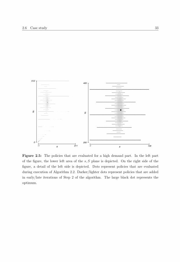
2.6 Case study 33
-1 3110
512
s
S
-1 149250
400
s
S
Figure 2.5: The policies that are evaluated for a high demand part. In the left part
of the figure, the lower left area of the s, S plane is depicted. On the right side of the
figure, a detail of the left side is depicted. Dots represent policies that are evaluated
during execution of Algorithm 2.2. Darker/lighter dots represent policies that are added
in early/late iterations of Step 2 of the algorithm. The large black dot represents the
optimum.
34 Spare parts inventory control for an aircraft component repair shop
businesses of Fokker Technologies, which develops and produces advanced structures and
electrical systems for the aviation and aerospace industry, and supplies integrated services
and products to aircraft owners and operators.
To explain the company’s motivation for implementing the method, we quote Maarten
van Marle, the managing director of the repair shop: “This project is important for Fokker
Services, as short and reliable repair turnaround times (TATs) are very important to our
customers when deciding to which repair shop they will outsource their repairs. Meeting
target TATs is therefore one of our primary KPIs. To score on this KPI, a number of
processes have to be under control. The most challenging of these processes is making
sure that the spare parts needed in the component repairs are available when we need
them, while at the same time keeping inventory costs under control.”
To give a better understanding of the importance of using automated methods for de-
termining (s, S) policies, we emphasize that inventory consists of a very broad assortment
of spare parts. As a consequence, each inventory analyst is responsible for the inventory
of a few thousand spare parts. Manually adjusting the policies to keep them up-to-date
with, for example, changes in repair volumes and supply leadtimes, is very time consum-
ing. Moreover, it is challenging to properly set the policies, while taking into account
both the need for short repair TATs and the need to keep inventory costs under control.
In order to use the algorithm in a DSS, data regarding the component repairs and
spare parts are needed. We now describe the approach that is used at the company to
obtain these data. Data are mainly retrieved from the ERP system of the repair shop.
Prices and leadtimes of spare parts are obtained in this manner. Future repair volumes
for the component types are estimated using econometric forecasting techniques. The
spare part usage probabilities P(Y ij = y) for each component are estimated based on data
regarding the spare parts usage in historic repairs. Due to regulation requirements, a long
history of accurate data regarding spare parts usage is available.
Because repair shops repair a wide range of component types, instances typically
consist of a large number of component types and spare parts. Case F in Table 2.1
corresponds to all components and spare parts used in one of the sections of the repair
shop, and thus gives an indication of the size of problems that are typically solved. Prices
vary between EUR 0.01 and 40,000, with 5% of the spare parts above EUR 2,500, and
80% below EUR 500. Leadtimes vary between a few days and 2 years, with 80% of the
leadtimes below 3 months. Forecasted repair rates of components types vary between 0
and 150 per year, and 80% of the components have a rate below 6 per year. Table 2.3
shows an example of an estimate of the spare part usage probabilities P(Y ij = y) for a
single component. Twenty-three of the twenty-nine parts are used with a probability that
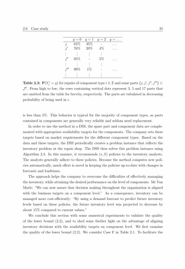
2.6 Case study 35
y = 0 y = 1 y = 2 y = . . .j 65% 35% - . . .j′ 76% 20% 4% . . ....
......
...j′′ 95% - 5% . . ....
......
...j′′′ 99% 1% - . . ....
......
...
Table 2.3: P(Y ij = y) for repairs of component type i ∈ I and some parts {j, j′, j′′, j′′′} ⊂
J i. From high to low, the rows containing vertical dots represent 3, 5 and 17 parts that
are omitted from the table for brevity, respectively. The parts are tabulated in decreasing
probability of being used in i.
is less than 5%. This behavior is typical for the majority of component types, as parts
contained in components are generally very reliable and seldom need replacement.
In order to use the method in a DSS, the spare part and component data are comple-
mented with appropriate availability targets for the components. The company sets these
targets based on market requirements for the different component types. Based on the
data and these targets, the DSS periodically creates a problem instance that reflects the
inventory problem at the repair shop. The DSS then solves this problem instance using
Algorithm 2.3. In this manner, it recommends (s, S) policies to the inventory analysts.
The analysts generally adhere to these policies. Because the method computes new poli-
cies automatically, much effort is saved in keeping the policies up-to-date with changes in
forecasts and leadtimes.
The approach helps the company to overcome the difficulties of effectively managing
the inventory, while attaining the desired performance on the level of components. Mr Van
Marle: “We can now assure that decision making throughout the organization is aligned
with the business targets on a component level.” As a consequence, inventory can be
managed more cost-efficiently: “By using a demand forecast to predict future inventory
levels based on these policies, the future inventory level was projected to decrease by
about 15% compared to current values.”
We conclude this section with some numerical experiments to validate the quality
of the lower bound (2.2), and to shed some further light on the advantage of aligning
inventory decisions with the availability targets on component level. We first examine
the quality of the lower bound (2.2). We consider Case F in Table 2.1. To facilitate the
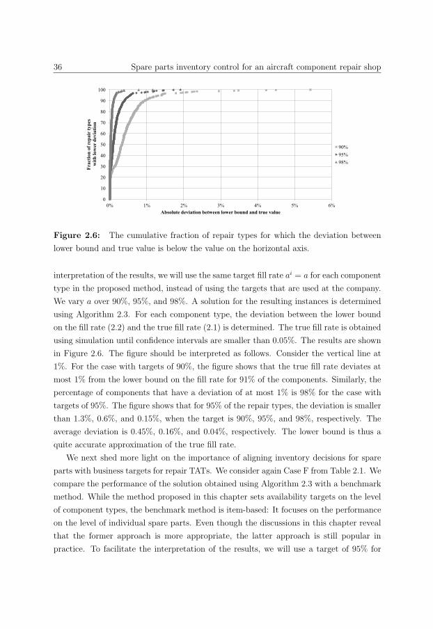
36 Spare parts inventory control for an aircraft component repair shop
0
10
20
30
40
50
60
70
80
90
100
0% 1% 2% 3% 4% 5% 6%
Frac
tion
of r
epai
r ty
pes
with
low
er d
evia
tion
Absolute deviation between lower bound and true value
90% 95% 98%
Figure 2.6: The cumulative fraction of repair types for which the deviation between
lower bound and true value is below the value on the horizontal axis.
interpretation of the results, we will use the same target fill rate ai = a for each component
type in the proposed method, instead of using the targets that are used at the company.
We vary a over 90%, 95%, and 98%. A solution for the resulting instances is determined
using Algorithm 2.3. For each component type, the deviation between the lower bound
on the fill rate (2.2) and the true fill rate (2.1) is determined. The true fill rate is obtained
using simulation until confidence intervals are smaller than 0.05%. The results are shown
in Figure 2.6. The figure should be interpreted as follows. Consider the vertical line at
1%. For the case with targets of 90%, the figure shows that the true fill rate deviates at
most 1% from the lower bound on the fill rate for 91% of the components. Similarly, the
percentage of components that have a deviation of at most 1% is 98% for the case with
targets of 95%. The figure shows that for 95% of the repair types, the deviation is smaller
than 1.3%, 0.6%, and 0.15%, when the target is 90%, 95%, and 98%, respectively. The
average deviation is 0.45%, 0.16%, and 0.04%, respectively. The lower bound is thus a
quite accurate approximation of the true fill rate.
We next shed more light on the importance of aligning inventory decisions for spare
parts with business targets for repair TATs. We consider again Case F from Table 2.1. We
compare the performance of the solution obtained using Algorithm 2.3 with a benchmark
method. While the method proposed in this chapter sets availability targets on the level
of component types, the benchmark method is item-based: It focuses on the performance
on the level of individual spare parts. Even though the discussions in this chapter reveal
that the former approach is more appropriate, the latter approach is still popular in
practice. To facilitate the interpretation of the results, we will use a target of 95% for
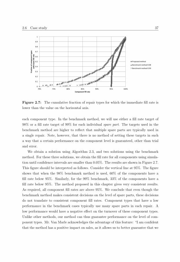
2.6 Case study 37
0
0.1
0.2
0.3
0.4
0.5
0.6
0.7
0.8
0.9
1
70% 75% 80% 85% 90% 95% 100%
Frac
tion
of c
ompo
nent
type
s w
ith lo
wer
fill
rate
Component fill rate
Proposed method
Benchmark method 0.98
Benchmark method 0.99
Figure 2.7: The cumulative fraction of repair types for which the immediate fill rate is
lower than the value on the horizontal axis.
each component type. In the benchmark method, we will use either a fill rate target of
98% or a fill rate target of 99% for each individual spare part. The targets used in the
benchmark method are higher to reflect that multiple spare parts are typically used in
a single repair. Note, however, that there is no method of setting these targets in such
a way that a certain performance on the component level is guaranteed, other than trial
and error.
We obtain a solution using Algorithm 2.3, and two solutions using the benchmark
method. For these three solutions, we obtain the fill rate for all components using simula-
tion until confidence intervals are smaller than 0.05%. The results are shown in Figure 2.7.
This figure should be interpreted as follows. Consider the vertical line at 95%. The figure
shows that when the 98% benchmark method is used, 60% of the components have a
fill rate below 95%. Similarly, for the 99% benchmark, 33% of the components have a
fill rate below 95%. The method proposed in this chapter gives very consistent results.
As required, all component fill rates are above 95%. We conclude that even though the
benchmark method makes consistent decisions on the level of spare parts, these decisions
do not translate to consistent component fill rates. Component types that have a low
performance in the benchmark cases typically use many spare parts in each repair. A
low performance would have a negative effect on the turnover of these component types.
Unlike other methods, our method can thus guarantee performance on the level of com-
ponent types. Mr. Van Marle acknowledges the advantage of this feature: “I am confident
that the method has a positive impact on sales, as it allows us to better guarantee that we
38 Spare parts inventory control for an aircraft component repair shop
deliver to our customers what they expect.” In terms of ordering and holding costs, the
proposed method also performs significantly better than the benchmark method. When
an individual fill rate target of 98% or 99% is used in the benchmark, costs are 36% or
52% higher than the costs of the proposed method, respectively.
Figure 2.7 also shows that the performance of many component types is significantly
above the 95% target in the proposed method. Figure 2.6 rules out the possibility that
this is caused by a poor performance of the lower bound. Instead, high availability of some
components is caused by a spill-over effect between the availability constraints of different
components that use similar spare parts, i.e., the constraints on some components are not
binding. An additional cause is the integrality of stock.
2.7 Conclusion
In this chapter, we propose a model for spare parts inventory control at a repair shop.
The difficulty of this problem is that performance is evaluated on the level of component
repairs, while inventory decisions are made for individual spare parts. We have formulated
this problem along the lines of existing models in the ATO literature. The theory devel-
oped in this chapter thus holds for general ATO systems, and consequently the solution
methodology directly translates to such systems.
The problem is formulated as a binary program, in which each combination of policy
parameters (s, S) is represented by a column. We solve the continuous relaxation of the
program by column generation and develop LP-based algorithms to find integer solutions.
As part of the column generation approach, we develop a very efficient algorithm to solve
the related pricing problem. Because the pricing problem is equivalent to single-item
policy optimization, this algorithm is interesting in its own right. It works under a very
general cost structure, and is able to take into account fill rate type of constraints. As
such, it works under more general conditions than existing algorithms.
The LP-based algorithms are the first optimization algorithms for ATO systems that
take into account the batching decision. They consider (s, S) policies instead of restrict-
ing attention to base-stock policies. The batching decision is important when ordering
costs are significant in comparison to holding costs, which is often the case for cheaper
components. In a computational study, we show that the algorithms find close-to-optimal
solutions for systems of the size that are prevalent in practice. They are the first algo-
rithms for ATO systems that are capable of solving such large-scale systems. Both the
capability of solving large-scale systems and the more general policy types contribute to
the applicability of the algorithm in practice, both for repair shops and for ATO systems.
2.A Proof of propositions 39
The method has been implemented at a repair shop owned by Fokker Services. In a case
study at the repair shop, we have shown that this implementation improves inventory
control. In particular, using the algorithm reduces the burden of periodically adapting
the inventory policies to changes in leadtimes and repair volumes. More importantly,
the algorithm aligns inventory decisions with business targets for the TATs of component
repairs. It significantly outperforms item-based approaches.
Appendices
‘
2.A Proof of propositions
Proof of Proposition 2.1 For the proof, we will use the following three lemmas.
Lemma 2.3 1. Hj(S − 1, S) is increasing in S.
2. F ij (S − 1, S) is decreasing in S.
Proof For fixed leadtime, evaluation of limt→∞ Ij(t) is standard. The results then follow
from (2.10) and (2.12). For stochastic sequential leadtimes, Hj(S−1, S) and F ij (S−1, S)
are evaluated by conditioning on the leadtime and using the approach for fixed leadtime
(cf. Zipkin (1986)). The asserted properties are preserved while conditioning. �
Lemma 2.4 1. Hj(s+Δ, S) and F ij (s−Δ, S) are nondecreasing in Δ.
2. Hj(s+Δ, S +Δ) and F ij (s−Δ, S −Δ)) are nondecreasing in Δ.
Proof The results are a consequence of (2.13) and the monotonicity of Hj(y − 1, y) and
F ij (y − 1, y) from Lemma 2.3. �
Lemma 2.5 Oj(S − s) is nonincreasing in S − s.
Proof Immediate from Oj(S − s) = ojλj/MS−s and the definition of MS−s. �Now, let (s, S) denote a policy in the parallelogram. By Lemma 2.4, we know that
H(s, S) ≥ H(s′, S ′), and F i(s, S) ≥ F i(s′′, S ′′), while Lemma 2.5 shows that O(s, S) ≥O(s′, S ′). Consequently, the reduced costs of (s, S) is bounded below by (2.20) (note
that νi ≥ 0). This proves the first claim. The additional claim follows immediately from
Lemma 2.4. This concludes the proof of Proposition 2.1.
40 Spare parts inventory control for an aircraft component repair shop
Proof of Proposition 2.2 Let j ∈ J be given and let (s, S) ∈ Cj be the policy to
control the inventory for spare part j. We will prove that
Hj(s, S) ≥ Hj
(s+ S − 1
2,s+ S + 1
2
),
where Hj(s, S) is the holding cost rate for part j.
We will apply renewal reward theory to compute the left-hand side. Renewals cor-
respond to moments at which a replenishment order is placed. Define C(s, S) as the
expected holding cost and T (s, S) as the expected time during a cycle. For simplicity
of notation, define pd = P(D = d) for d ∈ N as the compounding distribution for the
demand for spare part j. It then holds, that
C(s, S) =1
λj
Hj(S − 1, S) +S−s−1∑d=1
pdC(s, S − d), (2.26)
T (s, S) =1
λj
+S−s−1∑d=1
pdT (s, S − d). (2.27)
The elementary renewal theorem now states that
Hj(s, S) =C(s, S)
T (s, S)=
λjC(s, S)
λjT (s, S).
By this equation, we can assume λj = 1 without loss of generality. To ease the notation,
we now define
v : N→ R : n �→ v(n) = Hj
(s+
n
2, s+ 1 +
n
2
).
Hj(s − 12, s + 1
2) is defined as the average of Hj(s − 1, s) and Hj(s, s + 1) for all s ∈ Z.
Convexity of s �→ Hj(s, s+ 1) then implies that
Hj(i+ 1, i+ 2)−Hj(i, i+ 1) ≥ Hj(i, i+ 1)−Hj(i− 1, i)
for all i ∈ 12Z. The function v therefore satisfies
v(n+ 1)− v(n) ≥ v(n)− v(n− 1); (2.28)
i.e., the function v is convex. For later convenience, we also introduce
v : N20 → R : (i, j) �→ v(i, j) = v (i)− v (j) .
2.A Proof of propositions 41
(2.28) implies that the function i �→ v(i+1, i) is increasing. This implies that v(i+1, i) ≤v(j + 1, j) whenever i ≤ j. It follows for n, j ∈ N0 with 1 ≤ j ≤ n, that
v(n, n− j) = v (n)− v (n− j)
=
j−1∑k=0
v(n− k, n− k − 1) ≤j−1∑k=0
v(n, n− 1) = jv(n, n− 1).
As the left and right-hand side are obviously equal for j = 0, we conclude for 0 ≤ j ≤ n,
that
v(n, n− j) ≤ jv(n, n− 1). (2.29)
We will prove the lemma for fixed s by induction on S > s. Note that for fixed s, the
policy (s, S) is alternatively characterized by the difference S−s−1. To ease the notation,and to clarify the inductive argument, we define N = S−s−1 and apply the identification
N ∼ (s, s + 1 + N) ∈ Cj. Note that S > s is equivalent to N ≥ 0. We will apply the
following lemma.
Lemma 2.6 For all N ∈ N,∑N
j=1 jpjT (N − j) ≤ N.
Proof For N = 1 the result follows from the observation that p1 ≤ 1. Assume now that
it holds for all n < N . Then
N∑j=1
jpjT (N − j) = NpN +N−1∑j=1
jpjT (N − j) = NpN +N−1∑j=1
jpj
(1 +
N−j∑k=1
pkT (N − j − k)
)
=N∑j=1
jpj +N−1∑k=1
pk
N−k∑j=1
jpjT (N − k − j) ≤N∑j=1
jpj +N−1∑k=1
pk(N − k) =N∑j=1
Npj = N,
where the inequality relies on the induction hypothesis. This proves the claim. �We are now ready to prove Proposition 2.2. Recall that N = S − s− 1, so
v(N) = Hj
(2s+N
2,2s+ 2 +N
2
)= Hj
(s+ S − 1
2,s+ S + 1
2
).
Similarly v(2N) = Hj(S − 1, S). Using the notation introduced in this appendix, we
should thus prove the following.
Lemma 2.7 C(N)/T (N) ≥ v (N) for all N ∈ N0.
42 Spare parts inventory control for an aircraft component repair shop
Proof For N = 0 the result follows by definition. Assume now that it holds for all n < N .
We then have for all 1 ≤ j ≤ N
0 ≤ C(N − j)− v (N − j)T (N − j).
Multiplying this expression by pj and summing it from j = 1 to N , we obtain
0 ≤N∑j=1
pjC(N − j)−N∑j=1
pjv (N − j)T (N − j). (2.30)
Applying (2.29), Lemma 2.6 and monotonicity of i �→ v(i + 1, i), respectively, we see for
all 1 ≤ j ≤ N , that
N∑j=1
pj v(N,N − j)T (N − j) ≤ v(N,N − 1)N∑j=1
jpjT (N − j) ≤ Nv(N,N − 1)
≤N−1∑k=0
v(2N − k, 2N − k − 1) = v(2N)− v(N).
Rearranging terms, we can rewrite this as
0 ≤ v(2N)− v(N) +N∑j=1
pjv(N − j)T (N − j)−N∑j=1
pjv(N)T (N − j). (2.31)
Adding (2.30) and (2.31), we obtain
0 ≤ v(2N) +N∑j=1
pjC(N − j)− v(N)
(1 +
N∑j=1
pjT (N − j)
)= C(N)− v (N)T (N).
This proves the claim. �
Chapter 3
Optimization of industrial-scale
assemble-to-order systems
In this Chapter, we provide insights and algorithms to improve inventory control in
industrial-sized Assemble-To-Order (ATO) systems. By developing a novel stochastic
programming (SP) formulation, we develop an algorithm that has unparalleled efficiency
and scalability. Specifically, our algorithm can find tight bounds on optimal costs for
problems with hundreds of products and components, which enables us to prove that
our feasible solutions are within one percent of optimal. Our formulation allows us to
derive new insights with respect to the control and optimization of industrial-sized ATO
systems.
We consider a continuous time model in which we seek base-stock levels for compo-
nents, that minimize the sum of holding costs and product-specific backorder costs. Our
initial focus is on first-come first-serve (FCFS) allocation of components to products; for
this setting our algorithm quickly computes solutions that are provably within one percent
of the optimal base-stock/FCFS policy. We then turn to two related questions: How do
common heuristics used in practice compare to our performance, and how costly is the
FCFS assumption.
For the first question, we investigate the effectiveness of ignoring simultaneous stock-
outs (ISS), a heuristic that has been used by companies such as IBM and Dell to optimize
inventories. We show that ISS performance, when compared to the optimal FCFS base-
stock policy, increases as the average newsvendor (NV) fractiles increase. In addition,
lead time demand correlations have an adverse impact on ISS performance.
For the second question, we adapt the SP formulation of Dogru et al. (2010), yielding
an efficiently computable upper bound on the benefit of optimal allocation over FCFS.
We find that the performance of FCFS decreases with increasing NV fractile asymmetry
44 Optimization of industrial-scale assemble-to-order systems
among products and, again, with increasing average NV fractiles. For some important
cases, a large fraction of these benefits can be attained by combining simple no-holdback
allocation policies with the near-optimal base-stock levels (under FCFS) resulting from
our algorithm.
3.1 Introduction
Assemble-to-Order (ATO) systems allow companies to efficiently attain short response-
times for a broad assortment of products by assembling them, on demand, from multiple
components. But, to fully attain the benefits of ATO systems, companies need to effec-
tively control inventory for a large assortment of components. This is crucial, because
fulfillment depends on the simultaneous availability of the components that are needed to
assemble a demanded product, while a single component may be common for a number
of products (Song and Zipkin, 2003).
Specific examples of companies that manage large ATO-systems (i.e. with hundreds
of components) include IBM (Swaminathan and Tayur, 1998; Cheng et al., 2002) and
Dell (Kapuscinski et al., 2004). Online retailers and many maintenance organizations
face similar problems: The catalog of an online retailer may consist of thousands of
products. They often need to satisfy customer orders consisting of multiple products,
which should preferably be shipped together (e.g. Xu et al., 2009, at Amazon). Companies
that provide maintenance for capital goods typically keep inventories of many spare parts
and tools, repairs arriving over time typically require multiple spare parts and tools to
complete. Specific examples include the maintenance organizations of Philips Healthcare
(Kampstra, 2012), Fokker Services (Chapter 2 of this thesis), ASML (Vliegen, 2009) and
a copier manufacturer (Teunter, 2006). The assortments of Philips Healthcare and Fokker
Services, for example, consist of thousands of spare parts.
Companies typically cope with the difficulties of managing large-scale ATO systems
using pragmatic approaches. The replenishment process is generally simplified by control-
ling the inventory of each component independently. Also, companies often use first-come
first-serve (FCFS) allocation of components to products. Despite being non-optimal,
FCFS has many practical advantages such as ease of implementation and fairness. Also,
FCFS allows companies to guarantee a delivery date immediately upon demand arrival,
which is surprisingly difficult to achieve with other simple allocation policies (Lu et al.,
2010). When optimizing the component inventory control policies under FCFS, companies
may approximate the probability of stock-outs by Ignoring the possibility of Simultane-
ous Stock-outs (ISS). Companies using these pragmatic approaches have been described
3.1 Introduction 45
in various case studies (e.g. Cheng et al., 2002; Kapuscinski et al., 2004; Vliegen, 2009;
Xu et al., 2009). Chapter 2 of this thesis also gives a case study. The widespread use of
such strategies gives rise to a number of questions:
1. How to find provably (near-) optimal base-stock policies for FCFS ATO systems?
2. What are the costs of ignoring simultaneous stock-outs while optimizing the inven-
tory policy?
3. What are the costs of using FCFS instead of optimal allocation?
The goal of this chapter is to develop analytical models to address these questions, for
the first time, for the large-scale ATO systems that appear in practice.
While companies may use independent (r,Q) or (s, S) policies for inventory control
to attain economies of scale, most scholarly studies focus on base-stock policies, because
“it sharpens the focus on the higher-level business issue of inventory/service trade-off,
without getting into operational issues such as order sizes” (Song and Yao, 2002). We
focus on base-stock policies for the same reason. And, while many studies have addressed
the optimization of base-stock levels in FCFS ATO systems (e.g Zhang, 1997; Song and
Yao, 2002; Akcay and Xu, 2004; Lu et al., 2005; Lu and Song, 2005; Huang and De Kok,
2011) , none of the proposed methods can compute provably close-to-optimal solutions for
large-scale systems. This failure stems from not one, but two shortfalls: Current literature
not only lacks methods to find high quality solutions for large systems, but also cannot
provide tight lower bounds on the costs of the optimal solutions, which are necessary to
guarantee solution quality. We address both of these shortfalls by developing a novel,
exact, two-stage stochastic programming (SP) formulation that ensures that high quality
solutions and tight lower bounds are efficiently computable for large-scale systems. The
key to this efficiency is a formulation that yields second stage costs that are simply the
maximum of expressions that are linear in the first stage decision variables.
We consider systems in which the objective is to minimize the sum of component
holding and product-specific back-order costs. The SP we propose can be used to tackle
a range of modeling assumptions (see Proposition 3.3). But, for ease of presentation,
we focus on pure Poisson demand and deterministic lead-times. The approach we pro-
pose computes solutions that have optimality gaps that are smaller than one percent, for
problems consisting of many components and products.
Having answered our first question, we turn to the second: The performance of ISS
when compared to the optimal policy. Utilizing our tight lower bounds on optimal costs
under FCFS, we find that ISS has good performance when product newsvendor (NV)
46 Optimization of industrial-scale assemble-to-order systems
fractiles are high, but its performance degrades as NV fractiles decrease, especially when
leadtime demand for different components is highly correlated: Optimality losses in our
experiments range from 0.1 to 30%.
We then turn to our third question: What are the performance benefits of optimal
allocation when compared to FCFS? To answer this we develop an SP that constitutes a
lower bound on the costs of the optimal base-stock policy under optimal allocation. This
SP is obtained by adapting an idea proposed by Dogru et al. (2010) - minimizing the
cost rate incurred at a pre-specified moment in time, instead of minimizing the average
cost rate over time - to systems with unequal lead times. We are the first to employ
such methods for general ATO systems originating from industry, instead of focusing on
special cases.
Results for single-component systems may lead one to believe that NV fractile asym-
metry is the dominant factor determining the performance of FCFS (Topkis, 1968). While
it is true that as NV asymmetry increases, the relative benefit of optimal allocation over
FCFS increases, we find a number of practical cases in which this benefit remains rather
limited, even for significant NV asymmetry. For example, the relative benefit of optimal
allocation for a PC assembly case varies between 3− 8% depending on the NV fractiles,
and the relative benefit for assembly of products of multiple families varies between 3−8%or 8−18%, depending on whether product penalty asymmetry is between product families,
or within product families.
To investigate to what extent other simple allocation policies can close the gap between
the best FCFS policy and the lower bound under optimal allocation, we investigate two
easy-to-implement no-holdback policies: They always allocate components to a product
demand when this leads to demand fulfillment. We find that these allocation policies,
combined with suitable base-stock levels, can outperform the best possible FCFS policy by
up to 8%. Our new lower bound on the optimal FCFS policy is instrumental in obtaining
this result. No-holdback policies were investigated by other scholars (e.g. Song and Zhao,
2009; Lu et al., 2010; Dogru et al., 2010), who found promising results for special cases.
We appear to be the first to confirm their practical value for general systems.
In summary, we develop the first algorithm that computes provably near-optimal base-
stock levels for large, FCFS ATO systems. Using this algorithm we are able to generate
conclusive insights into the performance of the ISS heuristic for a number of industrial-
scale systems, allowing companies to infer whether ISS will perform well in their envi-
ronment. We then investigate the benefit of optimal allocation, other relatively simple
allocation rules, and optimal allocation, compared to FCFS in general industrial-sized
3.2 Literature review 47
ATO systems, deepening and expanding existing insights that were gained through the
study of small-scale systems and special cases.
The remainder of the chapter is organized as follows. In the next section we provide a
literature overview. In Section 3.3 we formulate our model, develop our SP formulation of
base-stock level optimization under FCFS, and computational procedures to solve it. We
also develop the lower bound on the optimal base-stock policy under optimal allocation.
In Section 3.4 we present the results of the computational study. We conclude in Section
3.5.
3.2 Literature review
Even though closed-form expressions of performance characteristics of ATO systems con-
trolled using base-stock policies and FCFS allocation often exist (e.g. Song, 1998, 2002;
Song et al., 1999), exact computation of these expressions is intractable for larger systems
(i.e. with more than 3 to 8 components in a product, depending on the precise setting).
As a consequence, scholars have developed bounds and approximations that are tractable
for larger systems (e.g. Song, 1998, 2002; Lu et al., 2003; Dayanik et al., 2003; Vliegen
and Van Houtum, 2009; Hoen et al., 2011). Such bounds have also been used to develop
approximate formulations of optimization problems (e.g. Zhang, 1997; Song and Yao,
2002; Cheng et al., 2002; De Kok, 2003; Lu et al., 2005; Lu and Song, 2005). The use of
the ISS assumption is an example along these lines: ISS gives rise to upper bounds on
waiting time (Lu and Song, 2005) and lower bounds on the fill-rate (Boole’s inequality).
We emphasize that while approximate formulations may be tractable, the resulting solu-
tion will be sub-optimal in general. Moreover, the degree of sub-optimality has remained
an open question, because of a lack of lower bounds on the optimal solution.
So, support of the use of ISS in practice has relied on arguments such those in Kapus-
cinski et al. (2004): “because the supply chain shortages of multiple components are very
infrequent, simultaneous stock-outs are rare and can be ignored.” However, Cheng et al.
(2002) find feasible solutions that improve costs by 8-15% for a 3 product system with
high fill-rate targets (in the 90-98% range). Similarly, while we show in Chapter 2 that
simultaneous stockouts are rare for the ISS solution, we cannot rule out the existence of
solutions that improve on the ISS solution.
We now review contributions considering the optimization of ATO systems, consider-
ing continuous review, periodic review, and then non-FCFS allocation.
Continuous review: Song and Yao (2002) develop algorithms for approximate mini-
mization of the number of back-orders in single product systems under iid lead-times. Lu
48 Optimization of industrial-scale assemble-to-order systems
et al. (2005) develop approximate formulations for the multi-product extension. Gullu and
Koksalan (2012) consider inventory control of orthopedic implants; where demand occurs
for kits of such implants. This problem is similar to ATO systems, but with a different
resupply system. A greedy heuristic is proposed to optimize the base-stock levels, which
is shown to have good performance in a numerical experiment. In Chapter 2, we study
the optimization of (s, S) policies at a repair shop. We develop an algorithm that finds
close-to-optimal solutions for large-scale problems formulated using the ISS assumption.
Our investigation into the quality of the ISS solutions (Question 2) builds on Lu and
Song (2005), who also consider cost minimization for product specific back-order costs,
focusing exclusively on FCFS allocation. For a 3-product 2-component system, they use
the closed-form expressions for the waiting time in Song (2002). For larger systems, they
rely on simulation and exhaustive search to identify good solutions. In these experiments,
they find solutions that outperform the ISS solution by 5%, and conclude that the ISS
solution has good performance. Our SP allows us to find provably near-optimal solutions
for large systems, which allows us to refine and modify Lu and Song’s (2005) conclusions.
Periodic review: The SP formulation due to Gerchak and Henig (1986) is one of the
first optimization methods for ATO systems, but is restricted to the single-period/zero-
leadtime case. Swaminathan and Tayur (1998) consider a case at IBM in which sub-
assemblies (vanilla boxes) play a pivotal role. They use heuristics and an SP solved using
a sub-gradient approach, again for the single-period/zero lead-time case.
For positive-leadtime models, different assumptions are studied regarding the alloca-
tion of components to products arriving in the same period, but all studies apply FCFS
to demands in different periods. Hausman et al. (1998) develop a heuristic which uses
an equal fill rate for each component. While this approach is simple, it cannot properly
account for differences in stock-out costs. Zhang (1997) assumes fixed priority allocation
and formulates an approximate optimization model for cost minimization under service
level constraints. Agrawal and Cohen (2001) derive similar results under a fair share
allocation rule. Cheng et al. (2002) minimize costs under product-specific fill rate con-
straints. They develop special purpose algorithms based on the ISS assumption, and
illustrate their approach on a case at IBM. De Kok (2003) considers ATO systems with
an ideal product structure: Longer lead-time components are either strictly more com-
mon, or completely independent of shorter lead-time components. He develops algorithms
to optimize base-stock levels based on approximations.
Akcay and Xu (2004) consider weighted time-window fill-rate maximization under a
budget constraint. Unlike the studies discussed earlier, they investigate the performance
of a heuristic that dynamically allocates components to products arriving in the same
3.2 Literature review 49
period, using an SP to optimize the base-stock levels. Huang and De Kok (2011) note
that many models exclude the holding costs of inventory committed to product demands.
Their model includes these committed inventory costs. Their computational results show
that committed stock may comprise a large fraction of total inventory. In addition, they
likewise develop an SP to optimize the base-stock levels. Both SP formulations (Akcay
and Xu, 2004; Huang and De Kok, 2011) are structurally similar to the SPs proposed
for the zero-leadtime case: They use the base-stock levels directly as decision variables,
which gives rise to a non-linear sampling-based problem (cf. Huang and De Kok, 2011).
To overcome this difficulty, they rely on binary auxiliary variables to linearize sampling-
based bounds, i.e. the big-M method (Huang and De Kok, 2011; Akcay and Xu, 2012) .
However, this approach gives rise to weak LP relaxations and severe scalability issues.
Our SP differs from existing SP formulations in a number of ways: We do not adapt
the zero lead time formulation by focusing on a specific period, but focus directly on an
arbitrary product demand. We determine the moment at which the components used in
that demand were ordered. In addition, we use binary variables that indicate that a par-
ticular base-stock level is used for a particular component demand, instead of using the
base-stock levels as decision variables. As a consequence, our SP gives rise to computa-
tional methods that do scale to large-scale systems, primarily because the sampling-based
lower bound has very strong linear relaxations.
Non-FCFS allocation: Optimal control in single-component systems requires ra-
tioning levels (Topkis, 1968), while optimal control of single product systems requires bal-
anced base-stock policies (Rosling, 1989). A particular multi -product, multi -component
system that has been of recent interest is the “W-model”: A 3-component 2-product
system, where one component is used in both products, while the other components are
each unique to a product. Bernstein et al. (2011) investigate a multi-period W-model,
with a single zero-leadtime replenishment. Other investigations typically assume multi-
ple replenishments and positive leadtimes: Song and Zhao (2009) compare the costs of
a single shared stock versus two separate stocks for the common component. Inventory
is controlled using base-stock policies. They find that first-ready first-serve (FRFS) allo-
cation, an example of a no-holdback policy, tends to outperform FCFS. Lu et al. (2010)
investigate base-stock control and no hold-back policies. They consider generalizations
of W-models: each product consists of a product specific component and a component
common to all products. They show that any no-holdback policy minimizes the total
back-orders and the total inventories, and thus total costs when back-order and holding
costs are symmetric.
50 Optimization of industrial-scale assemble-to-order systems
Dogru et al. (2010) study the W-model for product specific back-order costs, assuming
component lead-times are deterministic and equal. This is restrictive compared to the
general lead-time models in Lu et al. (2010). However, Dogru et al. (2010) obtain stronger
results: They develop a stochastic program that constitutes a lower bound on the costs of
any replenishment policy under optimal allocation, not restricted to the W-model. While
in general feasible solutions to the SP need not translate to feasible solutions to the original
problem, for the W-model under cost symmetry, they can translate an optimal solution to
this SP into a feasible (and optimal) solution for the original problem. The show that this
solution uses (independent) base-stock replenishment and no-holdback allocation. Under
a balanced capacity assumption, they prove the same result.
Each using a different proof technique, Lu et al. (2012) and Reiman and Wang (2012)
relax the equal lead-time condition. Lu et al. (2012) consider 2-component 2-product sys-
tems where one product uses both components, while the other product uses only a single
component (N-systems) with deterministic unequal leadtimes. Under cost symmetry, they
use a hybrid approach to show that the optimal policy is a coordinated base-stock policy
under no-holdback allocation. Reiman and Wang (2012) consider a generalized W-model:
Product specific components share the same lead-time, which is larger than the lead-time
of the common component. They adapt the SP formulation of Dogru et al. (2010) to
unequal lead-times. Under cost symmetry, they translate an optimal solution to the SP
into a feasible (and optimal) solution for the original problem. Replenishment involves
coordination, while no hold-back allocation remains optimal.
Other scholars have used dynamic programming to investigate the structure of the
optimal policy for Markovian ATO systems: Exponential make-to-stock replenishment,
Poisson demand, and lost sales. Benjaafar and ElHafsi (2006), ElHafsi et al. (2008), and
Nadar et al. (2011) study different system architectures; The latter allows products to use
different quantities of components. The general result is that optimal replenishment and
rationing decisions should take into account the inventory of all components. However,
while Benjaafar and ElHafsi (2006) and ElHafsi et al. (2008) find that state-dependent
base-stock levels and rationing levels are optimal, Nadar et al. (2011) show that still
more complex lattice-dependent base-stock policies and lattice dependent rationing is
optimal. Note that for these models, finding the optimal policy is only possible for very
small systems, because of the exponential growth of the state-space in the number of
components.
The general lesson is that optimal replenishment requires coordination of component
replenishment. An exception is Plambeck and Ward (2007), who assume that all prod-
ucts are delivered at their due date, by expediting components as needed. In that setting,
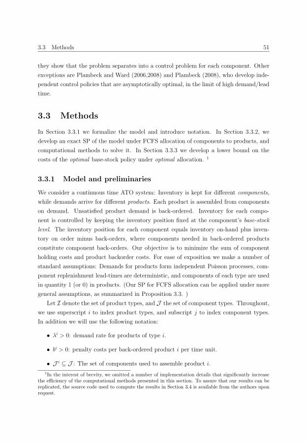
3.3 Methods 51
they show that the problem separates into a control problem for each component. Other
exceptions are Plambeck and Ward (2006,2008) and Plambeck (2008), who develop inde-
pendent control policies that are asymptotically optimal, in the limit of high demand/lead
time.
3.3 Methods
In Section 3.3.1 we formalize the model and introduce notation. In Section 3.3.2, we
develop an exact SP of the model under FCFS allocation of components to products, and
computational methods to solve it. In Section 3.3.3 we develop a lower bound on the
costs of the optimal base-stock policy under optimal allocation. 1
3.3.1 Model and preliminaries
We consider a continuous time ATO system: Inventory is kept for different components,
while demands arrive for different products. Each product is assembled from components
on demand. Unsatisfied product demand is back-ordered. Inventory for each compo-
nent is controlled by keeping the inventory position fixed at the component’s base-stock
level. The inventory position for each component equals inventory on-hand plus inven-
tory on order minus back-orders, where components needed in back-ordered products
constitute component back-orders. Our objective is to minimize the sum of component
holding costs and product backorder costs. For ease of exposition we make a number of
standard assumptions: Demands for products form independent Poisson processes, com-
ponent replenishment lead-times are deterministic, and components of each type are used
in quantity 1 (or 0) in products. (Our SP for FCFS allocation can be applied under more
general assumptions, as summarized in Proposition 3.3. )
Let I denote the set of product types, and J the set of component types. Throughout,
we use superscript i to index product types, and subscript j to index component types.
In addition we will use the following notation:
• λi > 0: demand rate for products of type i.
• bi > 0: penalty costs per back-ordered product i per time unit.
• J i ⊆ J : The set of components used to assemble product i.
1In the interest of brevity, we omitted a number of implementation details that significantly increasethe efficiency of the computational methods presented in this section. To assure that our results can bereplicated, the source code used to compute the results in Section 3.4 is available from the authors uponrequest.
52 Optimization of industrial-scale assemble-to-order systems
• Bi: random variable denoting the steady state number of back-ordered product i
demands.
• Ij ⊆ I: set of products that use a component j. So i ∈ Ij ⇔ j ∈ J i.
• hj > 0: holding costs per component j per unit time.
• lj > 0: lead time for replenishment orders of component j.
• l := maxj∈J lj: maximum replenishment leadtime.
• λj :=∑
i∈Ij λi: “demand” rate for components of type i.
• hi :=∑
j∈J i hj: “holding cost” for products of type i.
• Hj: random variable denoting the amount of on hand inventory of component j in
steady state (including committed inventory in the case of FCFS allocation).
• sj: base-stock level used for component type j; we assume sj ∈ {0, 1, 2, . . .}.
• �s := {sj|j ∈ J } : the vector of base-stock levels.
We consider the following cost rate:
∑i∈I
biE(Bi(�s)) +∑j∈J
hjE(Hj(�s)). (3.1)
For any allocation policy that does not let back-orders grow to infinity, the system is
positive recurrent, thus the expectations in (3.1) are well-defined. Apart from the base-
stock levels �s, Hj and Bi depend on the allocation policy that is used. In Section 3.3.2,
we investigate the minimization of (3.1) under the assumption of FCFS allocation of
components to product demands. In Section 3.3.3, we develop a lower bound on (3.1)
under optimal allocation.
Lu and Song (2005) show that (3.1) can be equivalently rewritten as
∑i∈I
biE(Bi(�s)) +∑j∈J
hjsj −D (3.2)
where bi = bi + hi and D =∑
j∈J hjλjlj. While Lu and Song (2005) restrict themselves
to FCFS allocation, the equivalence of (3.1) and (3.2) holds for any allocation policy.
3.3 Methods 53
-6.0 -5.0 -4.0 -3.0 -2.0 -1.0 0.0 1.0 2.0 3.0 4.0 5.0
Demand for product of type i ∈ I (t := 0)
= “Demand”for j ∈ J i
= “Demand”for j′ ∈ J i
t
W i = maxj∈J i W ij (sj)
123sj − 1sj
lj
W ij (sj)
T ij (sj)
12sj′
lj′
W ij′(sj′)
T ij′(sj′)
Figure 3.1: A graphical representation of T ij (k) and W i
j (k) and W i.
3.3.2 Base-stock levels under FCFS
In this section we propose a novel, exact SP formulation for minimization of the cost rate
(3.1) over the base-stock levels �s, when FCFS allocation is used. We develop a sampling
approximation of the SP. We then derive the ISS base-stock levels introduced by Lu and
Song (2005), and use the SP to prove that the ISS base-stock levels are upper bounds on
the optimal base-stock levels. Finally, we discuss how to extend the results in this section
to more general modeling assumptions.
Under FCFS, components are allocated to product demands in the order in which
the demands arrive: Upon arrival of a product demand that requires a component of
a certain type, an uncommitted on-hand component of that type is committed to that
product demand. If no such components are available, then the uncommitted component
on order that will arrive soonest is committed to the product demand.
The SP formulation and the ISS base-stock levels
Instead of focusing on the average number of back-orders Bi, our SP formulation is based
on the waiting time W i incurred by an arbitrary demand for a product of type i. Note
that EW i is a non-separable function of the base-stock levels of all components used in
product i.
Our first objective is to write W i as the maximum of a number of random variables,
that each depend on the base-stock level of only a single component. To this end, we
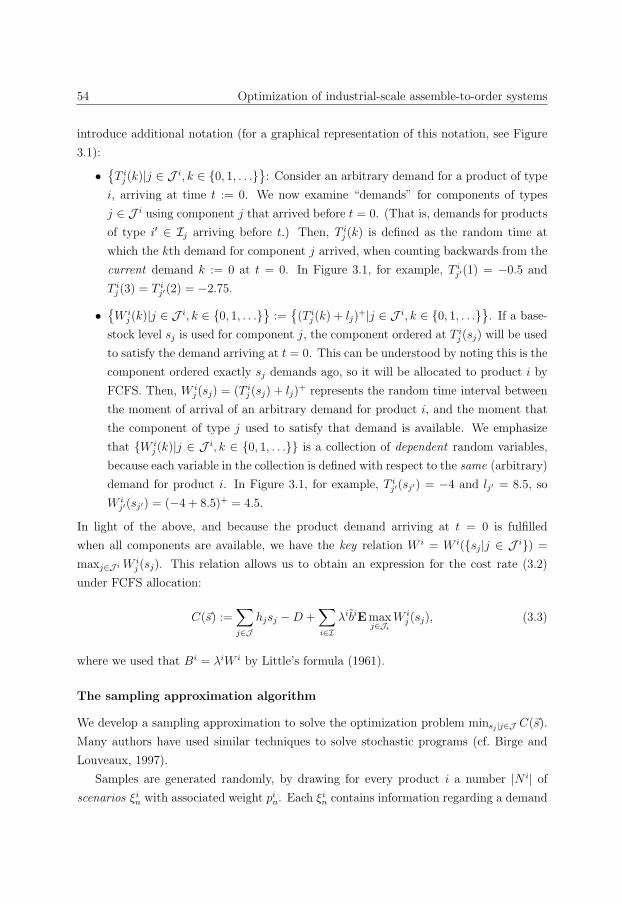
54 Optimization of industrial-scale assemble-to-order systems
introduce additional notation (for a graphical representation of this notation, see Figure
3.1):
• {T ij (k)|j ∈ J i, k ∈ {0, 1, . . .}}: Consider an arbitrary demand for a product of type
i, arriving at time t := 0. We now examine “demands” for components of types
j ∈ J i using component j that arrived before t = 0. (That is, demands for products
of type i′ ∈ Ij arriving before t.) Then, T ij (k) is defined as the random time at
which the kth demand for component j arrived, when counting backwards from the
current demand k := 0 at t = 0. In Figure 3.1, for example, T ij′(1) = −0.5 and
T ij (3) = T i
j′(2) = −2.75.
• {W ij (k)|j ∈ J i, k ∈ {0, 1, . . .}} := {(T i
j (k) + lj)+|j ∈ J i, k ∈ {0, 1, . . .}}. If a base-
stock level sj is used for component j, the component ordered at T ij (sj) will be used
to satisfy the demand arriving at t = 0. This can be understood by noting this is the
component ordered exactly sj demands ago, so it will be allocated to product i by
FCFS. Then, W ij (sj) = (T i
j (sj) + lj)+ represents the random time interval between
the moment of arrival of an arbitrary demand for product i, and the moment that
the component of type j used to satisfy that demand is available. We emphasize
that {W ij (k)|j ∈ J i, k ∈ {0, 1, . . .}} is a collection of dependent random variables,
because each variable in the collection is defined with respect to the same (arbitrary)
demand for product i. In Figure 3.1, for example, T ij′(sj′) = −4 and lj′ = 8.5, so
W ij′(sj′) = (−4 + 8.5)+ = 4.5.
In light of the above, and because the product demand arriving at t = 0 is fulfilled
when all components are available, we have the key relation W i = W i({sj|j ∈ J i}) =
maxj∈J i W ij (sj). This relation allows us to obtain an expression for the cost rate (3.2)
under FCFS allocation:
C(�s) :=∑j∈J
hjsj −D +∑i∈I
λibiEmaxj∈Ji
W ij (sj), (3.3)
where we used that Bi = λiW i by Little’s formula (1961).
The sampling approximation algorithm
We develop a sampling approximation to solve the optimization problem minsj |j∈J C(�s).
Many authors have used similar techniques to solve stochastic programs (cf. Birge and
Louveaux, 1997).
Samples are generated randomly, by drawing for every product i a number |N i| ofscenarios ξin with associated weight pin. Each ξin contains information regarding a demand
3.3 Methods 55
arrival for product i. In particular, ξin yields {W ij (s)(ξ
in)|j ∈ J i, s ∈ Sj}. Here, Sj :=
{0, . . . , suj } denotes the base-stock levels that may be optimal for (3.3) component i (see
Section 3.3.2). Samples should be drawn from a distribution that satisfies the following
condition:
EW i({sj|j ∈ J i}) = E∑n∈N i
pin maxj∈J i
W ij (sj)(ξ
in) ∀i, ∀sj ∈ Sj|j ∈ J i. (3.4)
We discuss how to generate samples in Appendix 3.A. Our approach for minimizing (3.3)
will be motivated by the following result.
Proposition 3.1 Let
Ca(�s) =∑j∈J
hjsj −D +∑i∈I
λibi∑n∈N i
pin maxj∈J i
W ij (sj)(ξ
in).
1. When samples are drawn to satisfy (3.4), then
E
(min
sj∈Sj |j∈JCa(�s)
)≤ min
sj∈Sj |j∈JC(�s) (3.5)
2. If in addition scenarios are drawn independently and weights satisfy pin = 1/|N i|,then
argminsj∈Sj |j∈J
Ca(�s) ⊆ argminsj∈Sj |j∈J
C(�s) (3.6)
with probability 1, as the number of scenarios grows large for each product.
(Proofs of all propositions are in Appendix 3.B.) Part 2 of the proposition implies that
solutions to minsj∈Sj |j∈J Ca(�s) for sufficiently large samples are likely to be of high quality
for (3.1) under FCFS. Of course, a question pertaining to this result is whether we are
able to compute solutions for samples consisting of sufficiently many scenarios. To answer
56 Optimization of industrial-scale assemble-to-order systems
this question, we will first formulate minsj∈Sj |j∈J Ca(�s) as a MIP:
min∑j∈J
∑s∈Sj
hjsxjs −D +∑i∈I
biλi∑n∈N i
pinvin, (3.7)
vin ≥∑s∈Sj
xjsWij (s)(ξ
in), i ∈ I, j ∈ J i, n ∈ N i, (3.8)
∑s∈Sj
xjs = 1, j ∈ J , (3.9)
vin ≥ 0, i ∈ I, n ∈ N i, (3.10)
xjs ∈ {0, 1}, j ∈ J , s ∈ Sj. (3.11)
The decision variables xjs indicate which base-stock levels are used: xjs = 1 implies that
sj = s. Hence, we need (3.9). The auxiliary real-valued decision variables vin represent
the waiting time incurred for sample ξin. Indeed, they take the minimum value allowed
by (3.8), which equals maxj∈J i W ij (sj)(ξ
ij) by the interpretation of xjs.
Our formulation uses indicator variables xjs. While it may appear that this makes
the problem more complex, it in fact significantly simplifies solving the problem. For
the modest price of adding 50 − 100 variables for each component (independent of the
number of scenarios in the sample), we linearize the constraints (3.8). The trade-off here
is very beneficial because modern MIP solvers scale to very large systems as long as the
LP relaxation is sufficiently strong. We found that the LP relaxation is very strong for
this problem: E.g., the root-node integrality gap is typically in the order of 0.5%.
To obtain good solutions, we took the component-wise average of the solution �s of (3.7-
3.11) for number of samples, and rounded each component to the nearest integer. We
estimate the objective value corresponding to this solution in an independent simulation
run. To assess whether the solution is close-to-optimal, we use Part 1 of Proposition 3.1:
We average minsj∈Sj |j∈J Ca(�s) for many independent samples to obtain a lower bound es-
timate, and use the variance of the objective values to construct an asymptotic confidence
interval for this estimate.
The ISS base-stock levels
An approximate optimization problem can be obtained by ignoring simultaneous stock-
outs (ISS) of multiple components in (3.3). If simultaneous stock-outs do not occur then
3.3 Methods 57
maxj Wij =∑
j Wij , which transforms (3.3) into
−D +∑j∈J
minsj∈{0,1,...}
⎛⎝hjsj +
∑i∈Ij
λibiEW ij (sj)
⎞⎠ (3.12)
The (highest) base-stock levels that minimize (3.12) will be referred to as the ISS solution
/base-stock levels. This solution was introduced as a heuristic by Lu and Song (2005). It
can be computed easily: (3.12) separates into a newsvendor problem for each component.
The ISS base-stock levels will be denoted by suj , j ∈ J because they are upper bounds on
the optimal base-stock levels under FCFS, as summarized in the following proposition.
(�s∨�s′ and �s∧�s′ denote the componentwise minimum and maximum of two vectors �s and
�s′, respectively. )
Proposition 3.2 Under FCFS allocation,
1. EW i(�s) and C(�s) are sub-modular in the base-stock levels sj: For any �s and �s′, it
holds that EW i(�s) + EW i(�s′) ≥ EW i(�s ∧ �s′) + EW i(�s ∨ �s′), and similar for C(·).
2. Each suj is an upper bound on the corresponding optimal base-stock level.
Lu and Song (2005) prove a similar result, and discuss an interesting economic interpreta-
tion of sub-modularity of the cost function: Inventories of components are complementary.
Our proof is different; we include it because it enables extensions such as non-unit usage of
components in products (see Proposition 3.3); Lu and Song (2005) discuss that extending
their method of proof to non-unit demand is difficult.
Extensions
The following proposition shows that results in this section can be extended to a (much)
more general setting.
Proposition 3.3 The cost formulation (3.3), the sample approximation (3.7-3.11), and
Proposition 3.2 can be extended to incorporate the following assumptions:
• Non-unit (possibly stochastic) requirements of components in products.
• Non-stationary demand for products.
• Make-to-stock, or stochastically sequential lead times (Svoronos and Zipkin, 1991).
• Exogenous batching of resupply orders, i.e. (r,Q) policies with Q exogenous.

58 Optimization of industrial-scale assemble-to-order systems
The results also extend when the costs biEBi in (3.2) are replaced by Eci(W i), for any
non-decreasing function ci(·). This allows the results to be extended to time window fill-
rate penalties.
3.3.3 A lower bound on the costs under optimal allocation
The purpose of this section is to develop an SP lower bound on the costs of the optimal
base-stock levels under optimal allocation. The SP lower bound we propose corresponds
to minimizing the (expected) cost rate (3.1) incurred at a pre-specified moment in time,
without taking into consideration the cost-rate before or after that point, instead of mini-
mizing the average cost rate over time. Dogru et al. (2010) and Reiman and Wang (2012)
use this idea to derive a lower bound for ATO systems. The SP we develop differs from
the SPs developed in Dogru et al. (2010) and Reiman and Wang (2012) because our SP
is two-stage, even for cases in which different components have different leadtimes, and
because our SP restricts attention to base-stock policies. Additionally, we increase compu-
tational efficiency by using a different formulation that halves the number of second-stage
decision variables.
Slightly abusing notation introduced in Section 3.3.1, we define the following:
• Di(t), for t > −l: Random demand for products of type i in period (−l, t]. For
convenience, let Dj(t) :=∑
i∈Ij Di(t).
• Bi(t): product i back-orders at t.
• Hj(0): on hand component j inventory at t = 0.
• zi: Total product demands of type i satisfied during (−l, 0]. This may include
demands that arrived before t− l.
We have the following relation:
Hj(0) = sj +∑i∈Ij
Bi(−l) +Dj(−lj)−∑i∈Ij
zi ≥ 0. (3.13)
This relation is valid because at −l, the inventory position of component type j is sj, while
back-orders equal∑
i∈Ij Bi(−l). (Because back-orders are subtracted from the inventory
position, additional inventory on-hand or on order is kept as a consequence of these back-
orders.) Also, “demand” Dj(−lj) arriving between −l and t − lj results in additional
purchase orders that arrive before 0. Finally, any satisfied product demands zi of type

3.4 Results 59
i ∈ Ij result in withdrawals of type j inventory. For product i back-orders at time 0 we
have:
Bi(0) = Bi(−l) +Di(0)− zi ≥ 0. (3.14)
For our SP, we take into account the constraints (3.13) and (3.14) that must be satisfied
by any base-stock policy under any allocation policy. Thus, the cost incurred at 0 depends
on the random variables Dj(−lj) and Di(0). We denote a realization of these random
variables (scenario) by ξ. Then, using (3.2), we find the following two-stage SP for cost
minimization at t := 0:
minsj≥0|j∈J
∑j∈J
hjsj −D + ECSP(�s, ξ). (3.15)
The second stage costs CSP(�s, ξ) are expressed in the decision variable xi := Bi(0) as
follows:
CSP(�s, ξ) =min∑i∈I
bixi, (3.16)
s.t.∑i∈Ij
xi + sj ≥ Dj(0)(ξ)−Dj(−lj)(ξ), (3.17)
0 ≤ xi ≤ Di(0)(ξ) +Bi(−l). (3.18)
Here, (3.17) and (3.18) correspond to (3.13) and (3.14), respectively. The minimization
is over xi and Bi(−l). Clearly, setting Bi(−l) =∞ will not affect the objective function,
so only xi remains as a second stage decision variable.
Because (3.1) is the average cost rate over time, while (3.15) minimizes the costs at
one point in time, (3.15) constitutes a lower bound on the cost rate (3.1) under optimal
allocation. This lower bound can in general not be attained by any feasible allocation
policy for (3.1).
To find upper and lower bounds to (3.15), we use a sampling-based approach, similar
to the approach described in Section 3.3.2 for solving (3.3). Details are available from the
authors on request.
3.4 Results
In this section, we use the algorithms developed in Section 3.3 to investigate the per-
formance of heuristic resupply and allocation rules commonly applied in industrial-scale
60 Optimization of industrial-scale assemble-to-order systems
ATO systems. We focus on the ISS heuristic to optimize the base-stock levels, and the
FCFS heuristic for allocation, though we also investigate other allocation heuristics. We
also investigate different methods for setting the base-stock levels. First, we summarize
the different policies that will be investigated. We then give the performance of these
policies from experiments with different ATO systems. Finally, we give a summary of
results and discuss the managerial insights gained though our study.
3.4.1 The investigated policies
Our main focus in this chapter will be on two simple policies; we will obtain performance
estimators for their associated average cost rate using simulation:
• iss-fc: The cost rate (3.1) incurred when applying the ISS base-stock levels and
FCFS allocation.
• spfc-fc: The cost rate (3.1) incurred when applying the SAA algorithm that uses
our exact SP formulation under FCFS (Section 3.3.2) to determine base-stock levels,
and FCFS allocation.
Clearly, estimators of the cost rates for iss-fc and spfc-fc alone give only limited insight
into the performance of these policies, because it is unclear what performance can be
hoped for. For that reason, we also developed estimators of lower bounds in Section 3.3:
• lb-fc: A lower bound on the best cost rate (3.1) that can be attained under FCFS
allocation of components to products and base-stock policies (Section 3.3.2 and
Proposition 3.1).
• lb-opt : A lower bound on the best cost rate (3.1) that can be attained under optimal
allocation of components to products, and base-stock policies (Section 3.3.3).
By comparing iss-fc and spfc-fc with lb-fc and lb-opt, we will be able to provide more
insightful results on the performance of those policies. Note that without the developments
in Section 3.3, we would not have been able to obtain these insights.
FCFS is not the only simple allocation rule that is applied in practice. Because other
scholars have found promising results for the relatively simple no-holdback allocation rules
in special cases (e.g. Song and Zhao, 2009; Dogru et al., 2010; Lu et al., 2010), we will
also investigate the performance of such rules. Under a no-holdback rule, components are
always allocated to a product demand if the allocation results in the fulfillment of that
demand. We test two different no-holdback rules that differ in the method by which back-
orders are cleared. The first-ready first-serve (FRFS) allocation rule clears back-orders
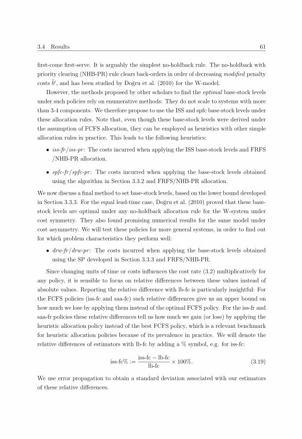
3.4 Results 61
first-come first-serve. It is arguably the simplest no-holdback rule. The no-holdback with
priority clearing (NHB-PR) rule clears back-orders in order of decreasing modified penalty
costs bi, and has been studied by Dogru et al. (2010) for the W-model.
However, the methods proposed by other scholars to find the optimal base-stock levels
under such policies rely on enumerative methods: They do not scale to systems with more
than 3-4 components. We therefore propose to use the ISS and spfc base-stock levels under
these allocation rules. Note that, even though these base-stock levels were derived under
the assumption of FCFS allocation, they can be employed as heuristics with other simple
allocation rules in practice. This leads to the following heuristics:
• iss-fr/iss-pr : The costs incurred when applying the ISS base-stock levels and FRFS
/NHB-PR allocation.
• spfc-fr/spfc-pr : The costs incurred when applying the base-stock levels obtained
using the algorithm in Section 3.3.2 and FRFS/NHB-PR allocation.
We now discuss a final method to set base-stock levels, based on the lower bound developed
in Section 3.3.3. For the equal lead-time case, Dogru et al. (2010) proved that these base-
stock levels are optimal under any no-holdback allocation rule for the W-system under
cost symmetry. They also found promising numerical results for the same model under
cost asymmetry. We will test these policies for more general systems, in order to find out
for which problem characteristics they perform well:
• drw-fr/drw-pr : The costs incurred when applying the base-stock levels obtained
using the SP developed in Section 3.3.3 and FRFS/NHB-PR.
Since changing units of time or costs influences the cost rate (3.2) multiplicatively for
any policy, it is sensible to focus on relative differences between these values instead of
absolute values. Reporting the relative difference with lb-fc is particularly insightful: For
the FCFS policies (iss-fc and saa-fc) such relative differences give us an upper bound on
how much we lose by applying them instead of the optimal FCFS policy. For the iss-fr and
saa-fr policies these relative differences tell us how much we gain (or lose) by applying the
heuristic allocation policy instead of the best FCFS policy, which is a relevant benchmark
for heuristic allocation policies because of its prevalence in practice. We will denote the
relative differences of estimators with lb-fc by adding a % symbol, e.g. for iss-fc:
iss-fc% :=iss-fc− lb-fc
lb-fc× 100%. (3.19)
We use error propagation to obtain a standard deviation associated with our estimators
of these relative differences.
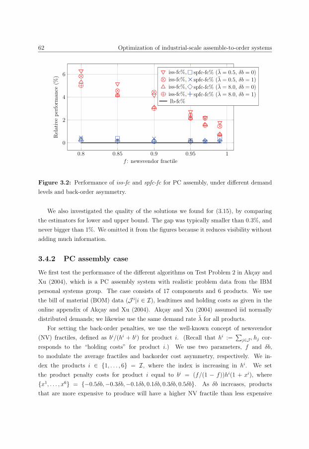
62 Optimization of industrial-scale assemble-to-order systems
0.8 0.85 0.9 0.95 1
0
2
4
6
f : newsvendor fractile
Relativeperform
ance
(%)
iss-fc%, spfc-fc% (λ = 0.5, δb = 0)
iss-fc%, spfc-fc% (λ = 0.5, δb = 1)
iss-fc%, spfc-fc% (λ = 8.0, δb = 0)
iss-fc%, spfc-fc% (λ = 8.0, δb = 1)lb-fc%
Figure 3.2: Performance of iss-fc and spfc-fc for PC assembly, under different demand
levels and back-order asymmetry.
We also investigated the quality of the solutions we found for (3.15), by comparing
the estimators for lower and upper bound. The gap was typically smaller than 0.3%, and
never bigger than 1%. We omitted it from the figures because it reduces visibility without
adding much information.
3.4.2 PC assembly case
We first test the performance of the different algorithms on Test Problem 2 in Akcay and
Xu (2004), which is a PC assembly system with realistic problem data from the IBM
personal systems group. The case consists of 17 components and 6 products. We use
the bill of material (BOM) data (J i|i ∈ I), leadtimes and holding costs as given in the
online appendix of Akcay and Xu (2004). Akcay and Xu (2004) assumed iid normally
distributed demands; we likewise use the same demand rate λ for all products.
For setting the back-order penalties, we use the well-known concept of newsvendor
(NV) fractiles, defined as bi/(hi + bi) for product i. (Recall that hi :=∑
j∈J i hj cor-
responds to the “holding costs” for product i.) We use two parameters, f and δb,
to modulate the average fractiles and backorder cost asymmetry, respectively. We in-
dex the products i ∈ {1, . . . , 6} = I, where the index is increasing in hi. We set
the product penalty costs for product i equal to bi = (f/(1 − f))hi(1 + xi), where
{x1, . . . , x6} = {−0.5δb,−0.3δb,−0.1δb, 0.1δb, 0.3δb, 0.5δb}. As δb increases, products
that are more expensive to produce will have a higher NV fractile than less expensive
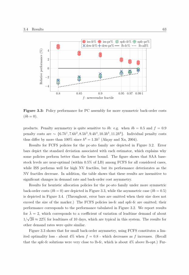
3.4 Results 63
0.8 0.85 0.9 0.95 0.97 0.99 1
−4
−2
0
2
4
f : newsvendor fractile
Relativeperform
ance
(%)
iss-fr% iss-pr% spfc-fr% spfc-pr%drw-fr% drw-pr% lb-fc% lb-all%
Figure 3.3: Policy performance for PC assembly for more symmetric back-order costs
(δb = 0).
products. Penalty asymmetry is quite sensitive to δb: e.g. when δb = 0.5 and f = 0.9
penalty costs are ∼ {6.7h1, 7.6h2, 8.5h3, 9.4h4, 10.3h5, 11.2h6}. Individual penalty costs
thus differ by more than 100% since h6 = 1.3h1 (Akcay and Xu, 2004).
Results for FCFS policies for the pc-ato family are depicted in Figure 3.2. Error
bars depict the standard deviation associated with each estimator, which explains why
some policies perform better than the lower bound. The figure shows that SAA base-
stock levels are near-optimal (within 0.5% of LB) among FCFS for all considered cases,
while ISS performs well for high NV fractiles, but its performance deteriorates as the
NV fractiles decrease. In addition, the table shows that these results are insensitive to
significant changes in demand rate and back-order cost asymmetry.
Results for heuristic allocation policies for the pc-ato family under more symmetric
back-order costs (δb = 0) are depicted in Figure 3.3, while the asymmetric case (δb = 0.5)
is depicted in Figure 3.4. (Throughout, error bars are omitted when their size does not
exceed the size of the marker.) The FCFS policies iss-fc and spfc-fc are omitted; their
performance corresponds to the performance tabulated in Figure 3.2. We report results
for λ = 2, which corresponds to a coefficient of variation of leadtime demand of about
1/√20 ≈ 22% for leadtimes of 10 days, which are typical in this system. The results for
other demand rates were quite similar.
Figure 3.3 shows that for small back-order asymmetry, using FCFS constitutes a lim-
ited optimality loss - about 4% when f = 0.8 - which decreases as f increases. (Recall
that the spfc-fc solutions were very close to lb-fc, which is about 4% above lb-opt.) Fur-
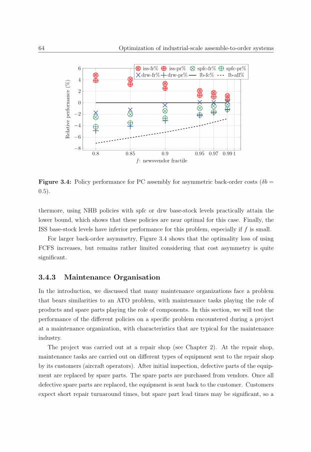
64 Optimization of industrial-scale assemble-to-order systems
0.8 0.85 0.9 0.95 0.97 0.99 1−8−6−4−20
2
4
6
f : newsvendor fractile
Relativeperform
ance
(%)
iss-fr% iss-pr% spfc-fr% spfc-pr%drw-fr% drw-pr% lb-fc% lb-all%
Figure 3.4: Policy performance for PC assembly for asymmetric back-order costs (δb =
0.5).
thermore, using NHB policies with spfc or drw base-stock levels practically attain the
lower bound, which shows that these policies are near optimal for this case. Finally, the
ISS base-stock levels have inferior performance for this problem, especially if f is small.
For larger back-order asymmetry, Figure 3.4 shows that the optimality loss of using
FCFS increases, but remains rather limited considering that cost asymmetry is quite
significant.
3.4.3 Maintenance Organisation
In the introduction, we discussed that many maintenance organizations face a problem
that bears similarities to an ATO problem, with maintenance tasks playing the role of
products and spare parts playing the role of components. In this section, we will test the
performance of the different policies on a specific problem encountered during a project
at a maintenance organization, with characteristics that are typical for the maintenance
industry.
The project was carried out at a repair shop (see Chapter 2). At the repair shop,
maintenance tasks are carried out on different types of equipment sent to the repair shop
by its customers (aircraft operators). After initial inspection, defective parts of the equip-
ment are replaced by spare parts. The spare parts are purchased from vendors. Once all
defective spare parts are replaced, the equipment is sent back to the customer. Customers
expect short repair turnaround times, but spare part lead times may be significant, so a
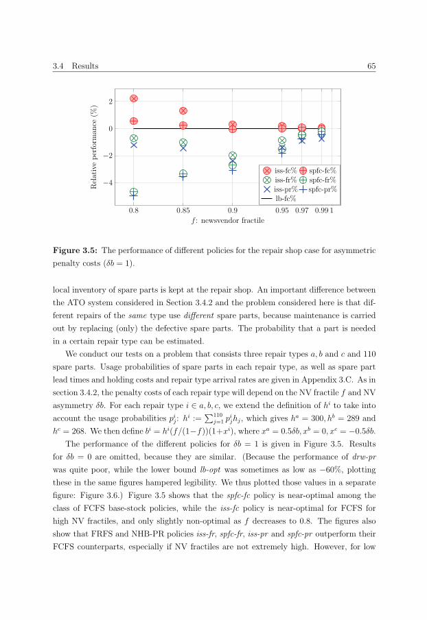
3.4 Results 65
0.8 0.85 0.9 0.95 0.97 0.99 1
−4
−2
0
2
f : newsvendor fractile
Relativeperform
ance
(%)
iss-fc% spfc-fc%iss-fr% spfc-fr%iss-pr% spfc-pr%lb-fc%
Figure 3.5: The performance of different policies for the repair shop case for asymmetric
penalty costs (δb = 1).
local inventory of spare parts is kept at the repair shop. An important difference between
the ATO system considered in Section 3.4.2 and the problem considered here is that dif-
ferent repairs of the same type use different spare parts, because maintenance is carried
out by replacing (only) the defective spare parts. The probability that a part is needed
in a certain repair type can be estimated.
We conduct our tests on a problem that consists three repair types a, b and c and 110
spare parts. Usage probabilities of spare parts in each repair type, as well as spare part
lead times and holding costs and repair type arrival rates are given in Appendix 3.C. As in
section 3.4.2, the penalty costs of each repair type will depend on the NV fractile f and NV
asymmetry δb. For each repair type i ∈ a, b, c, we extend the definition of hi to take into
account the usage probabilities pij: hi :=∑110
j=1 pijhj, which gives ha = 300, hb = 289 and
hc = 268. We then define bi = hi(f/(1−f))(1+xi), where xa = 0.5δb, xb = 0, xc = −0.5δb.The performance of the different policies for δb = 1 is given in Figure 3.5. Results
for δb = 0 are omitted, because they are similar. (Because the performance of drw-pr
was quite poor, while the lower bound lb-opt was sometimes as low as −60%, plotting
these in the same figures hampered legibility. We thus plotted those values in a separate
figure: Figure 3.6.) Figure 3.5 shows that the spfc-fc policy is near-optimal among the
class of FCFS base-stock policies, while the iss-fc policy is near-optimal for FCFS for
high NV fractiles, and only slightly non-optimal as f decreases to 0.8. The figures also
show that FRFS and NHB-PR policies iss-fr, spfc-fr, iss-pr and spfc-pr outperform their
FCFS counterparts, especially if NV fractiles are not extremely high. However, for low
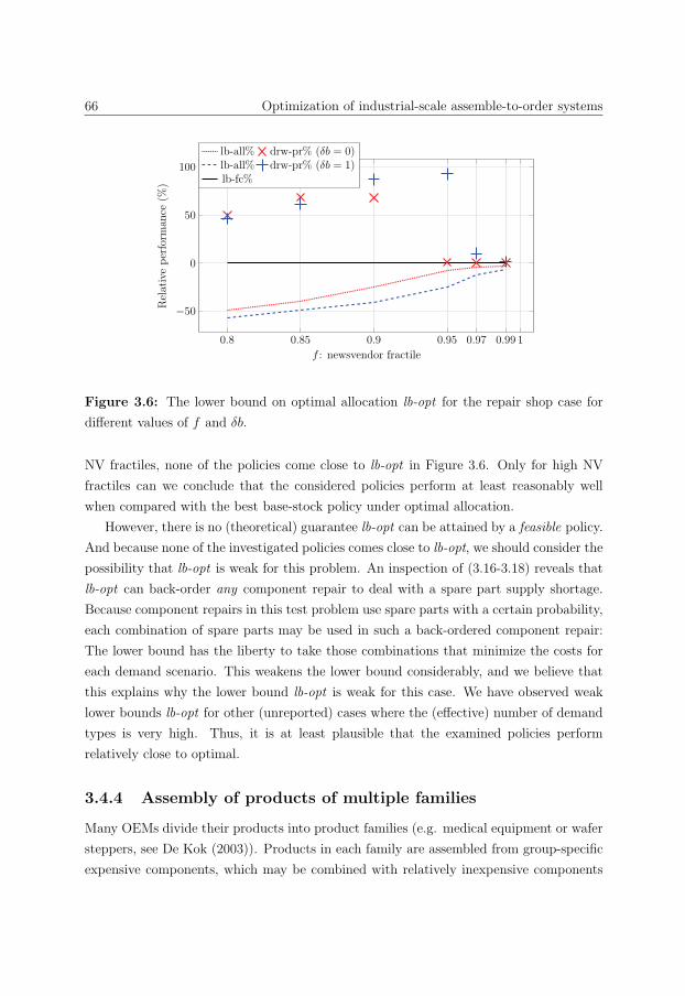
66 Optimization of industrial-scale assemble-to-order systems
0.8 0.85 0.9 0.95 0.97 0.99 1
−50
0
50
100
f : newsvendor fractile
Relativeperform
ance
(%)
lb-all% drw-pr% (δb = 0)lb-all% drw-pr% (δb = 1)lb-fc%
Figure 3.6: The lower bound on optimal allocation lb-opt for the repair shop case for
different values of f and δb.
NV fractiles, none of the policies come close to lb-opt in Figure 3.6. Only for high NV
fractiles can we conclude that the considered policies perform at least reasonably well
when compared with the best base-stock policy under optimal allocation.
However, there is no (theoretical) guarantee lb-opt can be attained by a feasible policy.
And because none of the investigated policies comes close to lb-opt, we should consider the
possibility that lb-opt is weak for this problem. An inspection of (3.16-3.18) reveals that
lb-opt can back-order any component repair to deal with a spare part supply shortage.
Because component repairs in this test problem use spare parts with a certain probability,
each combination of spare parts may be used in such a back-ordered component repair:
The lower bound has the liberty to take those combinations that minimize the costs for
each demand scenario. This weakens the lower bound considerably, and we believe that
this explains why the lower bound lb-opt is weak for this case. We have observed weak
lower bounds lb-opt for other (unreported) cases where the (effective) number of demand
types is very high. Thus, it is at least plausible that the examined policies perform
relatively close to optimal.
3.4.4 Assembly of products of multiple families
Many OEMs divide their products into product families (e.g. medical equipment or wafer
steppers, see De Kok (2003)). Products in each family are assembled from group-specific
expensive components, which may be combined with relatively inexpensive components
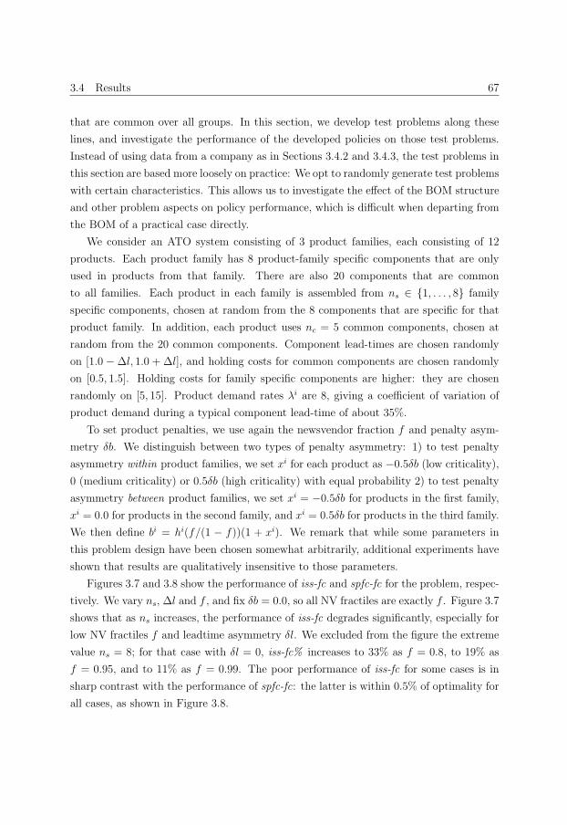
3.4 Results 67
that are common over all groups. In this section, we develop test problems along these
lines, and investigate the performance of the developed policies on those test problems.
Instead of using data from a company as in Sections 3.4.2 and 3.4.3, the test problems in
this section are based more loosely on practice: We opt to randomly generate test problems
with certain characteristics. This allows us to investigate the effect of the BOM structure
and other problem aspects on policy performance, which is difficult when departing from
the BOM of a practical case directly.
We consider an ATO system consisting of 3 product families, each consisting of 12
products. Each product family has 8 product-family specific components that are only
used in products from that family. There are also 20 components that are common
to all families. Each product in each family is assembled from ns ∈ {1, . . . , 8} family
specific components, chosen at random from the 8 components that are specific for that
product family. In addition, each product uses nc = 5 common components, chosen at
random from the 20 common components. Component lead-times are chosen randomly
on [1.0 −Δl, 1.0 + Δl], and holding costs for common components are chosen randomly
on [0.5, 1.5]. Holding costs for family specific components are higher: they are chosen
randomly on [5, 15]. Product demand rates λi are 8, giving a coefficient of variation of
product demand during a typical component lead-time of about 35%.
To set product penalties, we use again the newsvendor fraction f and penalty asym-
metry δb. We distinguish between two types of penalty asymmetry: 1) to test penalty
asymmetry within product families, we set xi for each product as −0.5δb (low criticality),
0 (medium criticality) or 0.5δb (high criticality) with equal probability 2) to test penalty
asymmetry between product families, we set xi = −0.5δb for products in the first family,
xi = 0.0 for products in the second family, and xi = 0.5δb for products in the third family.
We then define bi = hi(f/(1 − f))(1 + xi). We remark that while some parameters in
this problem design have been chosen somewhat arbitrarily, additional experiments have
shown that results are qualitatively insensitive to those parameters.
Figures 3.7 and 3.8 show the performance of iss-fc and spfc-fc for the problem, respec-
tively. We vary ns, Δl and f , and fix δb = 0.0, so all NV fractiles are exactly f . Figure 3.7
shows that as ns increases, the performance of iss-fc degrades significantly, especially for
low NV fractiles f and leadtime asymmetry δl. We excluded from the figure the extreme
value ns = 8; for that case with δl = 0, iss-fc% increases to 33% as f = 0.8, to 19% as
f = 0.95, and to 11% as f = 0.99. The poor performance of iss-fc for some cases is in
sharp contrast with the performance of spfc-fc: the latter is within 0.5% of optimality for
all cases, as shown in Figure 3.8.
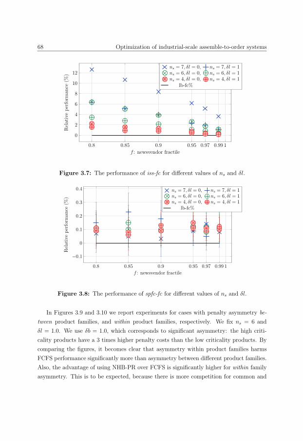
68 Optimization of industrial-scale assemble-to-order systems
0.8 0.85 0.9 0.95 0.97 0.99 1
0
2
4
6
8
10
12
f : newsvendor fractile
Relativeperform
ance
(%)
ns = 7, δl = 0, ns = 7, δl = 1ns = 6, δl = 0, ns = 6, δl = 1ns = 4, δl = 0, ns = 4, δl = 1
lb-fc%
Figure 3.7: The performance of iss-fc for different values of ns and δl.
0.8 0.85 0.9 0.95 0.97 0.99 1
−0.1
0
0.1
0.2
0.3
0.4
f : newsvendor fractile
Relativeperform
ance
(%)
ns = 7, δl = 0, ns = 7, δl = 1ns = 6, δl = 0, ns = 6, δl = 1ns = 4, δl = 0, ns = 4, δl = 1
lb-fc%
Figure 3.8: The performance of spfc-fc for different values of ns and δl.
In Figures 3.9 and 3.10 we report experiments for cases with penalty asymmetry be-
tween product families, and within product families, respectively. We fix ns = 6 and
δl = 1.0. We use δb = 1.0, which corresponds to significant asymmetry: the high criti-
cality products have a 3 times higher penalty costs than the low criticality products. By
comparing the figures, it becomes clear that asymmetry within product families harms
FCFS performance significantly more than asymmetry between different product families.
Also, the advantage of using NHB-PR over FCFS is significantly higher for within family
asymmetry. This is to be expected, because there is more competition for common and
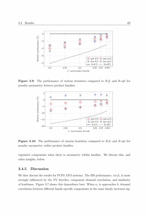
3.4 Results 69
0.8 0.85 0.9 0.95 0.97 0.99 1
−8
−6
−4
−2
0
f : newsvendor fractile
Relativeperform
ance
(%)
spfc-fr% spfc-pr%drw-fr% drw-pr%lb-fc% lb-all%
Figure 3.9: The performance of various heuristics compared to lb-fc and lb-opt for
penalty asymmetry between product families.
0.8 0.85 0.9 0.95 0.97 0.99 1−20
−15
−10
−5
0
5
f : newsvendor fractile
Relativeperform
ance
(%)
spfc-fr% spfc-pr%drw-fr% drw-pr%lb-fc% lb-all%
Figure 3.10: The performance of various heuristics compared to lb-fc and lb-opt for
penalty asymmetry within product families.
expensive components when there is asymmetry within families. We discuss this, and
other insights, below.
3.4.5 Discussion
We first discuss the results for FCFS ATO systems. The ISS performance, iss-fc, is most
strongly influenced by the NV fractiles, component demand correlation, and similarity
of leadtimes. Figure 3.7 shows this dependence best: When ns is approaches 8, demand
correlation between different family-specific components in the same family increases sig-
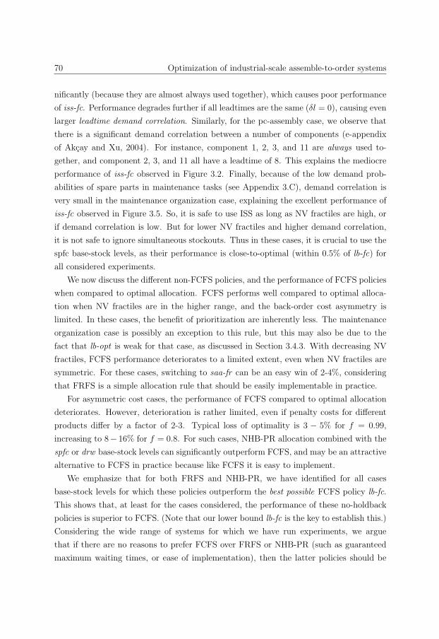
70 Optimization of industrial-scale assemble-to-order systems
nificantly (because they are almost always used together), which causes poor performance
of iss-fc. Performance degrades further if all leadtimes are the same (δl = 0), causing even
larger leadtime demand correlation. Similarly, for the pc-assembly case, we observe that
there is a significant demand correlation between a number of components (e-appendix
of Akcay and Xu, 2004). For instance, component 1, 2, 3, and 11 are always used to-
gether, and component 2, 3, and 11 all have a leadtime of 8. This explains the mediocre
performance of iss-fc observed in Figure 3.2. Finally, because of the low demand prob-
abilities of spare parts in maintenance tasks (see Appendix 3.C), demand correlation is
very small in the maintenance organization case, explaining the excellent performance of
iss-fc observed in Figure 3.5. So, it is safe to use ISS as long as NV fractiles are high, or
if demand correlation is low. But for lower NV fractiles and higher demand correlation,
it is not safe to ignore simultaneous stockouts. Thus in these cases, it is crucial to use the
spfc base-stock levels, as their performance is close-to-optimal (within 0.5% of lb-fc) for
all considered experiments.
We now discuss the different non-FCFS policies, and the performance of FCFS policies
when compared to optimal allocation. FCFS performs well compared to optimal alloca-
tion when NV fractiles are in the higher range, and the back-order cost asymmetry is
limited. In these cases, the benefit of prioritization are inherently less. The maintenance
organization case is possibly an exception to this rule, but this may also be due to the
fact that lb-opt is weak for that case, as discussed in Section 3.4.3. With decreasing NV
fractiles, FCFS performance deteriorates to a limited extent, even when NV fractiles are
symmetric. For these cases, switching to saa-fr can be an easy win of 2-4%, considering
that FRFS is a simple allocation rule that should be easily implementable in practice.
For asymmetric cost cases, the performance of FCFS compared to optimal allocation
deteriorates. However, deterioration is rather limited, even if penalty costs for different
products differ by a factor of 2-3. Typical loss of optimality is 3 − 5% for f = 0.99,
increasing to 8− 16% for f = 0.8. For such cases, NHB-PR allocation combined with the
spfc or drw base-stock levels can significantly outperform FCFS, and may be an attractive
alternative to FCFS in practice because like FCFS it is easy to implement.
We emphasize that for both FRFS and NHB-PR, we have identified for all cases
base-stock levels for which these policies outperform the best possible FCFS policy lb-fc.
This shows that, at least for the cases considered, the performance of these no-holdback
policies is superior to FCFS. (Note that our lower bound lb-fc is the key to establish this.)
Considering the wide range of systems for which we have run experiments, we argue
that if there are no reasons to prefer FCFS over FRFS or NHB-PR (such as guaranteed
maximum waiting times, or ease of implementation), then the latter policies should be
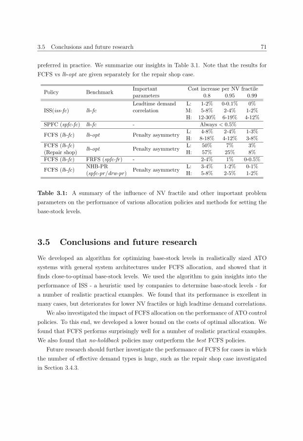
3.5 Conclusions and future research 71
preferred in practice. We summarize our insights in Table 3.1. Note that the results for
FCFS vs lb-opt are given separately for the repair shop case.
Policy BenchmarkImportant Cost increase per NV fractileparameters 0.8 0.95 0.99
ISS(iss-fc) lb-fcLeadtime demand L: 1-2% 0-0.1% 0%correlation M: 5-8% 2-4% 1-2%
H: 12-30% 6-19% 4-12%
SPFC (spfc-fc) lb-fc - Always < 0.5%
FCFS (lb-fc) lb-opt Penalty asymmetryL: 4-8% 2-4% 1-3%H: 8-18% 4-12% 3-8%
FCFS (lb-fc)lb-opt Penalty asymmetry
L: 50% 7% 3%(Repair shop) H: 57% 25% 8%
FCFS (lb-fc) FRFS (spfc-fr) - 2-4% 1% 0-0.5%
FCFS (lb-fc)NHB-PR
Penalty asymmetryL: 3-4% 1-2% 0-1%
(spfc-pr/drw-pr) H: 5-8% 2-5% 1-2%
Table 3.1: A summary of the influence of NV fractile and other important problem
parameters on the performance of various allocation policies and methods for setting the
base-stock levels.
3.5 Conclusions and future research
We developed an algorithm for optimizing base-stock levels in realistically sized ATO
systems with general system architectures under FCFS allocation, and showed that it
finds close-to-optimal base-stock levels. We used the algorithm to gain insights into the
performance of ISS - a heuristic used by companies to determine base-stock levels - for
a number of realistic practical examples. We found that its performance is excellent in
many cases, but deteriorates for lower NV fractiles or high leadtime demand correlations.
We also investigated the impact of FCFS allocation on the performance of ATO control
policies. To this end, we developed a lower bound on the costs of optimal allocation. We
found that FCFS performs surprisingly well for a number of realistic practical examples.
We also found that no-holdback policies may outperform the best FCFS policies.
Future research should further investigate the performance of FCFS for cases in which
the number of effective demand types is huge, such as the repair shop case investigated
in Section 3.4.3.
72 Optimization of industrial-scale assemble-to-order systems
Appendices
3.A Sample generation
By simulating the ATO system and inspecting Tij(k) upon arrival of a demand for prod-
uct i, we can obtain realizations of the original random variable {W ij (s)|j ∈ J i, s ∈ Sj},
giving us scenarios ξin. Because leadtimes are deterministic, a warm-up period of l before
taking samples is sufficient. Because experiments indicated that (significant) dependence
adversely impacts the quality of the bounds, we skip n orders for product i before draw-
ing each scenario for that product, where n is chosen such that the probability that two
drawings occur within l is negligible. (We cannot simply skip l because of the inspection
paradox.) Because a sample consisting of scenarios of the original random variable obvi-
ously satisfies (3.4), such samples are used in many SAAs, typically with equal weights
pin = 1/|N i|.However, when newsvendor fractiles are (moderately) high, most scenarios ξin from the
original distribution are boring : They give zero associated waiting time W i(ξin) for any
solution �s of reasonable quality. A small fraction of scenarios are interesting: It is more
likely that they give a positive waiting time for reasonable solutions. As a consequence,
we need a huge number of scenarios from the original distribution to obtain reasonable
lower bounds. But solving the SAA for such large samples is time-consuming, especially
for large systems. We propose a simple yet effective method to generate skewed samples,
i.e. samples with a large fraction of interesting scenarios: 1) Generate a large number of
scenarios; 2) Use a heuristic to divide the scenarios into interesting and boring scenarios;
3) (Randomly) drop the majority of boring scenarios; 4) Adapt the weight of the remaining
boring scenarios, to ensure that condition (3.4) holds.
The approach will generate valid samples regardless of the heuristic used in step 2,
but a low quality heuristic will not improve the quality of the samples. Our heuristic first
determines base-stock levels with reasonable quality by solving (3.7-3.11) for a standard
sample with equal weights. This is repeated for a small number (five) of independent sam-
ples, �s is chosen as the component-wise minimum of the resulting solutions. (The solution
values for these five samples are not used in any statistics.) We are then ready to generate
skewed samples: A scenarios ξ is qualified as boring if and only if W i(ξ)(�s) = 0. Samples
generated in this manner give rise to superior lower and upper bounds, when compared
with samples of the same size consisting of independent equal-weight realizations.
3.B Proof of propositions 73
3.B Proof of propositions
In this appendix, we provide the proofs of the propositions in Section 3.3.
Proof of Proposition 3.1. 1) See Mak et al. (1999, Theorem 1).
2) Let �s /∈ argminC(�s). Then C(�s) = C(�s′) + 2ε with ε > 0 for some �s′, because the
argmin is over a finite set. But this gives
P[�s ∈ argminCa(�s)] ≤ P[Ca(�s) ≤ Ca(�s′)]
≤ (P[|Ca(�s)− C(�s)| ≥ ε] +P[|Ca(�s′)− C(�s′)| ≥ ε]),
which approaches 0 as |N i| → ∞ for all i by the weak law of large numbers. (Note that
Emaxj∈J i W ij (sj)(ξ
in) = EW i({sj|j ∈ J i}) by (3.4).)
This proof extends to the sampling scheme proposed in Appendix 3.A, because the
central limit continues to guarantee P(|Ca(�s)− C(�s)| > ε)→ 0.
Proof of Proposition 3.2. 1) We proof a slightly more general result, to facilitate the
extensions in Proposition 3.3: We will prove that Eci(W i) is submodular for any non-
decreasing function ci(·). By definition of T ij , we know that W i
j is non-increasing in sj,
which implies for every scenario ξ that
∀sj ≤ s′j : ci(W i
j (sj)(ξ)) ≥ ci(W ij (s
′j)(ξ)). (3.20)
In addition, the key insight of Section 3.3.2 implies that
ci(W i(ξ)) = maxj∈J i
ci(W ij (sj)(ξ)). (3.21)
It is easy to verify that (3.20) and (3.21) imply that ci(W i(ξ(ω))) is sub-modular in
the base-stock levels. Because taking expectations preserves sub-modularity, Eci(W i)
is sub-modular (see e.g. Topkis, 1998). Submodularity of C follows from (3.3) because
taking linear combinations with positive weights preserves sub-modularity, and because
the holding costs are linear, and hence submodular, in the base-stock levels.
2) It is well-known that sub-modularity of C implies that component inventory is
complementary: The cost-minimizing base-stock level for each part is nondecreasing in
the base-stock level of other parts (Topkis, 1998). Thus, if we let all sj′ with j′ = j
approach infinity, then the resulting cost-minimizing base-stock level sj for component
j is an upper bound on the optimal base-stock level for that component. But sj′ → ∞implies P (W i
j′(sj′) = 0) → 1. As a consequence, it can be verified from (3.3) that
74 Optimization of industrial-scale assemble-to-order systems
the cost minimization problem for sj approaches minsj hjsj +∑
i∈Ij λibiEW i
j (sj), which
corresponds to the ISS minimization problem (3.12) for component j.
Proof of Proposition 3.3. We mention where the extensions require non-trivial adapta-
tions of methods and/or proofs.
The reader may verify that equivalence of (3.1) and (3.2) continues to hold with
an appropriate redefinition of bi and D. In all cases, D should correct for the average
difference between inventory level and inventory position. When components are used
stochastically in products, bi and Bi are dependent : bi ends up inside the expectation in
(3.2).
The key relation derived in Section 3.3.2 is easily adapted to the various mentioned
extensions. For non-unit component usage in products, W ij (k) should be redefined to
the waiting time for the last component of type j to become available for the product i
demand. For stochastic component usage, waiting times depend on how many components
are needed in each specific product demand; components that are not needed in a specific
product should be excluded from the maximum. When exogenous batching is applied,
W ij (k) needs to take into account which component in the batch is used to satisfy the last
demand. Any changes in the modeling assumptions can and should be taken into account
during sampling.
The proof of Proposition 3.2 extends because it only uses the key relation derived in
Section 3.3.2, and that W ij (k) is decreasing in k for every sample, which clearly continues
to hold for all extensions. So the ISS base-stock levels can be generalized for the various
extensions, and remain upper bounds to the optimal base-stock levels.
Validity of the key relation and (3.21) also assures that the sampling approximation
(3.7-3.11) remains valid. Because bi is inside the expectation for stochastic requirements
of components in products, it will depend on the specific scenario for those cases.
3.C Data for the maintenance organization problem
Data for the maintenance organization problem are given in this section. The problem
data were estimated based on data in the ERP system of the company, see Chapter 2.
Costs and lead-times have been rescaled and rounded to prevent any sensitive information
from being retrievable from the data. This did not affect the main insights gained through
this study.
The case consists of three repair types a, b and c, with associated arrival rates 0.13, 0.10
and 0.35 per unit of time, respectively. Spare parts are characterized by their lead time
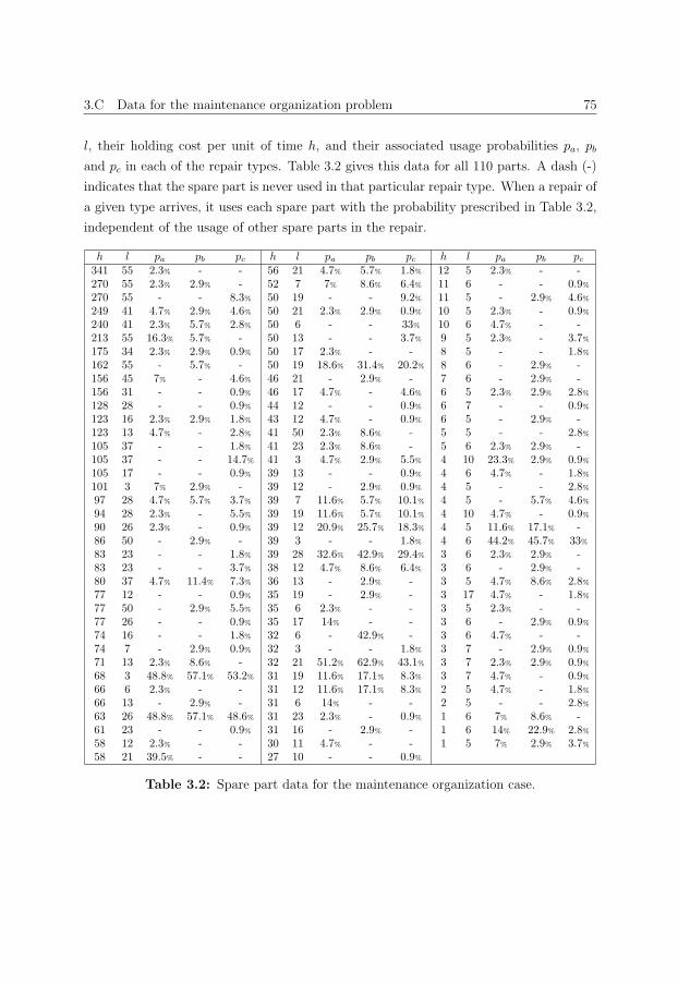
3.C Data for the maintenance organization problem 75
l, their holding cost per unit of time h, and their associated usage probabilities pa, pb
and pc in each of the repair types. Table 3.2 gives this data for all 110 parts. A dash (-)
indicates that the spare part is never used in that particular repair type. When a repair of
a given type arrives, it uses each spare part with the probability prescribed in Table 3.2,
independent of the usage of other spare parts in the repair.
h l pa pb pc h l pa pb pc h l pa pb pc341 55 2.3% - - 56 21 4.7% 5.7% 1.8% 12 5 2.3% - -270 55 2.3% 2.9% - 52 7 7% 8.6% 6.4% 11 6 - - 0.9%270 55 - - 8.3% 50 19 - - 9.2% 11 5 - 2.9% 4.6%249 41 4.7% 2.9% 4.6% 50 21 2.3% 2.9% 0.9% 10 5 2.3% - 0.9%
240 41 2.3% 5.7% 2.8% 50 6 - - 33% 10 6 4.7% - -213 55 16.3% 5.7% - 50 13 - - 3.7% 9 5 2.3% - 3.7%
175 34 2.3% 2.9% 0.9% 50 17 2.3% - - 8 5 - - 1.8%162 55 - 5.7% - 50 19 18.6% 31.4% 20.2% 8 6 - 2.9% -156 45 7% - 4.6% 46 21 - 2.9% - 7 6 - 2.9% -156 31 - - 0.9% 46 17 4.7% - 4.6% 6 5 2.3% 2.9% 2.8%128 28 - - 0.9% 44 12 - - 0.9% 6 7 - - 0.9%123 16 2.3% 2.9% 1.8% 43 12 4.7% - 0.9% 6 5 - 2.9% -123 13 4.7% - 2.8% 41 50 2.3% 8.6% - 5 5 - - 2.8%105 37 - - 1.8% 41 23 2.3% 8.6% - 5 6 2.3% 2.9% -105 37 - - 14.7% 41 3 4.7% 2.9% 5.5% 4 10 23.3% 2.9% 0.9%105 17 - - 0.9% 39 13 - - 0.9% 4 6 4.7% - 1.8%
101 3 7% 2.9% - 39 12 - 2.9% 0.9% 4 5 - - 2.8%97 28 4.7% 5.7% 3.7% 39 7 11.6% 5.7% 10.1% 4 5 - 5.7% 4.6%94 28 2.3% - 5.5% 39 19 11.6% 5.7% 10.1% 4 10 4.7% - 0.9%
90 26 2.3% - 0.9% 39 12 20.9% 25.7% 18.3% 4 5 11.6% 17.1% -86 50 - 2.9% - 39 3 - - 1.8% 4 6 44.2% 45.7% 33%
83 23 - - 1.8% 39 28 32.6% 42.9% 29.4% 3 6 2.3% 2.9% -83 23 - - 3.7% 38 12 4.7% 8.6% 6.4% 3 6 - 2.9% -80 37 4.7% 11.4% 7.3% 36 13 - 2.9% - 3 5 4.7% 8.6% 2.8%77 12 - - 0.9% 35 19 - 2.9% - 3 17 4.7% - 1.8%
77 50 - 2.9% 5.5% 35 6 2.3% - - 3 5 2.3% - -77 26 - - 0.9% 35 17 14% - - 3 6 - 2.9% 0.9%74 16 - - 1.8% 32 6 - 42.9% - 3 6 4.7% - -74 7 - 2.9% 0.9% 32 3 - - 1.8% 3 7 - 2.9% 0.9%71 13 2.3% 8.6% - 32 21 51.2% 62.9% 43.1% 3 7 2.3% 2.9% 0.9%68 3 48.8% 57.1% 53.2% 31 19 11.6% 17.1% 8.3% 3 7 4.7% - 0.9%
66 6 2.3% - - 31 12 11.6% 17.1% 8.3% 2 5 4.7% - 1.8%
66 13 - 2.9% - 31 6 14% - - 2 5 - - 2.8%63 26 48.8% 57.1% 48.6% 31 23 2.3% - 0.9% 1 6 7% 8.6% -61 23 - - 0.9% 31 16 - 2.9% - 1 6 14% 22.9% 2.8%58 12 2.3% - - 30 11 4.7% - - 1 5 7% 2.9% 3.7%58 21 39.5% - - 27 10 - - 0.9%
Table 3.2: Spare part data for the maintenance organization case.


Chapter 4
A Two-step Method for Forecasting
Spare Parts Demand using
Information on Component Repairs
Forecasting spare parts demand is notoriously difficult, as demand is typically intermittent
and lumpy. Specialized methods such as that by Croston are available, but these are not
based on the repair operations that cause the intermittency and lumpiness of demand. In
this chapter, we do propose a method that, in addition to the demand for spare parts,
considers the type of component repaired. This two-step forecasting method separately
updates the average number of parts needed per repair and the number of repairs for
each type of component. The method is tested in an empirical, comparative study for a
service provider in the aviation industry. Our results show the two step method is one
of the most accurate methods, and that it performs considerably better than Croston’s
method. Moreover, contrary to other methods, the two-step method can use information
on planned maintenance and repair operations to reduce forecasts errors by up to 20%. We
derive further analytical and simulation results that help explain the empirical findings.
4.1 Introduction
This chapter is, in the first place, motivated by the problem of forecasting spare parts
demand at Fokker Services, a company that maintains and repairs aircraft components.
Fokker Services is one of the five businesses of Fokker Technologies, which develops and
produces advanced structures and electrical systems for the aviation and aerospace in-
dustry, and supplies integrated services and products to aircraft owners and operators.
78 Forecasting Spare Parts Demand using Information on Component Repairs
At Fokker Services, expensive spare parts have to be stocked in order to quickly carry
out repairs. Therefore, forecasting demand is an important issue at Fokker, and more
generally in the spare part industry. Boone et al. (2008) reports from a Delphi study with
senior service part managers that demand forecasting is the key challenge in service parts
management. Better forecasting techniques might reduce safety stocks and thus might
reduce costs without reducing service levels.
Fokker Services has detailed data over a ten year period that links spare parts demand
to the type of component repaired, and the number of spare parts used per component
repair. This raises the interesting question of whether this link can be used to more
accurately forecast demand. Standard forecasting methods, such as exponential smooth-
ing and moving average, as well as specialized methods such as that by Croston (1972),
only consider demand for spare parts and not the underlying repair process. However,
that repair process does, in part, cause the intermittent and lumpy demand patterns that
complicate spare parts forecasting. In this chapter, we propose a new, so-called two-step
forecasting method that does take the additional repair information into account. In the
first step we forecast, for each type of component, the number of repairs per time unit of
that component and the number of spare parts (of the type under consideration) needed
per repair of that component. In the second step, these forecasts are combined to fore-
cast total demand for a spare part. The rationale behind this method is that the ability
to recognize what causes a change in the demand for spare parts, contrary to existing
methods, should lead to better demand forecasts. For instance, a drop in demand for a
spare part at Fokker Services may result either from aircrafts being taken out of use, or
from finding new ways (based on improved technology) of repairing rather than replacing
parts of a failed component. In this example, the former case will imply a reduction in
the number of repairs for certain components, while the latter will affect the number of
parts needed per repair.
We use the data set of Fokker Services to compare the two-step methods with several
traditional methods, such as exponential smoothing, moving average, Croston’s method,
and a recently proposed method by Teunter et al. (2011). Based on the mean square
error (MSE), mean absolute deviation (MAD), and mean error (ME), we conclude that
the two-step method is one of the best performing methods, and that it considerably
outperforms the well-known Croston method. Furthermore, by taking information on the
planning of maintenance and repair operations into account, the forecasts errors of the
two step method can be reduced by up to 20%. Other methods cannot benefit from this
information as they do not link demand at the part level to specific repair operations.
4.2 Literature review 79
The remainder of this chapter is organized as follows. Section 4.2 gives an overview
of the relevant literature. Section 4.3 describes the data and in Section 4.4 the various
forecasting methods are introduced. Section 4.5 summarizes the results of our case study
and in Section 4.6 a simulation study gives insights into the differences between the new
two step method and exponential smoothing. Finally, we give some concluding remarks
and directions for future research in Section 4.7.
4.2 Literature review
We restrict ourselves in this review to forecasting demand, we refer to Guide and Sri-
vastava (1997) and Kennedy et al. (2002) for more general overviews on spare parts
management. In fact, we concentrate on the forecasting contributions that are most rel-
evant for our study and refer to Boylan and Syntetos (2010) for a comprehensive review
on forecasting spare parts demand.
Forecasting demand has been an important issue for many years. Traditional methods
include moving average and exponential smoothing, see e.g. Axsater (2006). Exponential
smoothing in particular has shown itself to be a very robust forecast method that is
able to adapt quickly to changes in the demand process, and it is widely used in practice.
However, Croston (1972) has shown that both exponential smoothing and moving average
do not perform well for intermittent demand, i.e. when there are many periods with zero
demand. He proposes to update the demand size and the demand interval separately using
exponential smoothing. Updates are only carried out in periods with positive demands.
Syntetos and Boylan (2001) show that Croston’s method is biased and suggest an ad-
justment to overcome this issue in a follow-up paper (Syntetos and Boylan (2005)). Other
variants of Croston’s method are suggested in the literature as well. In a comparative
study, Teunter and Sani (2009) show that the variants of Syntetos (2001) and Syntetos
and Boylan (2005) are the most promising ones. Other studies compare variants of Cros-
ton’s method with traditional methods; see e.g. Willemain et al. (1994), Ghobbar and
Friend (2003), and Eaves and Kingman (2004). These studies show that most variants
outperform traditional methods on average, but not for all possible situations.
Teunter et al. (2011) show that the Croston approach is not suited to deal with obso-
lescence issues. They propose to update the demand probability instead of the demand
interval. The advantage is that the demand probability can be updated every period,
whereas the demand interval can only be updated in a period with a positive demand.
Bootstrapping offers a non-parametric alternative for forecasting spare parts demand.
Similar to the above discussed methods, forecasts are based purely on the demand history.
80 Forecasting Spare Parts Demand using Information on Component Repairs
However, rather then specifying a certain updating structure for the forecast and asso-
ciated forecasting error, sample statistics are used to estimate the demand distribution.
Bootstrapping methods range from very simple (Efron (1979); Porras and Dekker (2008))
to more complex (Willemain et al. (2004)).
Some authors have also considered to use types of information other than historic
demand, such as installed base information (Song and Zipkin (1996a); Jalil et al. (2011)),
reliability information (Petrovic and Petrovic (1992)) and expert judgment (Syntetos et al.
(2009)). Wang and Syntetos (2011) discuss a maintenance based model for forecasting
spare part demand which uses information on the demand generation process. However,
they do not take into account that spare parts might be used in the repair for various
types of components. To the best of our knowledge, no methods have previously been
proposed that make use of information on the type of component whose repair generated
the demand for a spare part, as we do in this study.
4.3 Data description
The data set contains information on over 100,000 repairs at Fokker Services during the
period from 01-01-2000 until 28-02-2010. For each repair the date of issue, the type of
component that is repaired, and the spare parts used are recorded. Some repairs do not
require any spare parts, others require many spare parts of various types. In total 3,329
different types of components are repaired, and 17,012 different types of spare parts are
used during these repairs. Forecasting at Fokker Services is carried out on a monthly basis
and this is typical in the service industry. Therefore, monthly aggregates are created.
The first seven years, i.e., the period from 01-01-2000 until 31-12-2006, represents the
initialization period. This is about two-third of the total period, similar as in Teunter and
Duncan (2009). During this period the forecasting methods are initialized; see Subsection
4.4.1. Note that spare parts that are not demanded during the initialization period are
left out of consideration.
Spare parts are categorized based on the number of months with positive demand
during the initialization period. The three categories are very-slow moving (1-5 months
with positive demand), slow moving (6-20 months), and fast moving (21-84 months). We
could have created further categories by considering the lumpiness of the demand size as
well (as in Syntetos et al. (2005)), but preliminary tests showed demand ‘speed’ to have the
most significant effect on the comparative results that we study. The choice of boundaries
between the three categories is somewhat arbitrary, but ensures in line with traditional
ABC analysis that the slowest moving category contains the largest number of parts and
4.4 Forecasting methods 81
the fastest moving category contains the smallest number of parts. Furthermore, different
boundaries that we considered produced similar results to those that we will present.
Table 4.1 gives an overview of the three categories.
very-slow moving slow moving fast movingNumber of part types 6,015 2,865 1,696avg monthly demand 0.0514 0.340 3.134avg annual number of demands 0.301 1.541 5.735
Table 4.1: An overview of the three spare part categories. All statistics are calculated
using the aggregate monthly data during the initialization period.
4.4 Forecasting methods
In this section, all considered forecasting methods are described. Table 4.2 gives an
overview of these methods and their abbreviations. Many methods are well known and
serve as a benchmark against which our two-step method is tested.
Table 4.2: The forecasting methods used and their abbreviations.
Abbreviation MethodZF Zero ForecastNF Naive ForecastMA Moving Average ForecastES Exponential Smoothing ForecastCR Croston’s Forecasting MethodSBA Syntetos-Boylan ApproximationTSB Teunter-Syntetos-Babai Forecasting Method2S Two Step Forecast
All methods forecast monthly demand for each type of spare part separately. There-
fore, we use the phrase demand instead of demand for spare parts of type i throughout this
section. First, we give an overview of the notation that we will use, with abbreviations of
related methods between brackets.
xt forecast at the beginning of month t of demand in month t;
dt demand in month t;
kt forecast in month t of number of months between consecutive positive demands
(CR, SBA);
82 Forecasting Spare Parts Demand using Information on Component Repairs
kt number of months since the last positive demand at the beginning of month t (CR,
SBA);
st forecast of demand in month t, provided this demand is positive (CR, SBA, TSB);
pt forecast of the probability of a positive demand in month t (TSB);
pt indicator variable that indicates whether or not there is a positive demand in month
t (TSB);
xct forecast of demand in month t used for components of type c (2S);
dct demand in month t used for components of type c (2S);
zct forecast of number of repairs of components of type c in month t (2S);
zct number of repairs of components of type c in month t (2S);
act forecast of the average number of spare parts used in month t for the repair of a
component of type c (2S);
α, β smoothing constants (0 ≤ α, β ≤ 1);
Zero Forecast (ZF) and Naive Forecast (NF)
The first two methods are very simple benchmark methods. The zero forecast (ZF)
always predicts zero. This is an effective method for forecasting intermittent demand
when performance measures such as the mean square error (MSE) and mean absolute
deviation (MAD) are used. However, this forecasting method is of no use when applied
in an inventory control setting; see Teunter and Duncan (2009). The naive forecast (NF)
uses the last observation as the forecast. This method can be considered a special case of
other forecasting methods such as, for example, ES and MA.
Moving Average Forecast (MA)
The moving average forecast (MA) is the mean of the previous N months. That is,
xt+1 =1
N
N∑i=1
dt−N+i.
Exponential Smoothing Forecast (ES)
The exponential smoothing forecast (ES) uses the demand in month t and the forecast
for month t to predict demand in month t+ 1. The ES forecast is
xt+1 = (1− α)xt + αdt, (4.1)
where 0 ≤ α ≤ 1 is the smoothing constant.
4.4 Forecasting methods 83
Croston’s Forecasting Method (CR)
Croston (1972) argues that for intermittent demand patterns, MA and ES do not per-
form well. He proposes to update the demand size, st+1, and the demand interval, kt+1,
separately, using
st+1 =
{st, if dt = 0
(1− α)st + αdt, if dt > 0,
and
kt+1 =
{kt, if dt = 0
(1− β)kt + βkt, if dt > 0,
where 0 ≤ α, β ≤ 1. The Croston forecast (CR) is
xt+1 =st+1
kt+1
.
Syntetos-Boylan Approximation (SBA)
As discussed in the introduction, Syntetos and Boylan (2001) show that Croston’s method
is positively biased. To approximately correct for that bias, they propose to deflate the
Croston forecast by a factor 1− α/2. So, the SBA forecast is
xt+1 = (1− α
2)st+1
kt+1
.
Forecasting Method of Teunter et al. (2011) (TSB)
Teunter et al. (2011) propose an alternative to Croston’s method that is able to handle
obsolescence issues. They do not update the demand interval, but rather the probability
of a positive demand. This probability and the demand size are updated using,
st+1 =
{st, if dt = 0
(1− α)st + αdt, if dt > 0,
and
pt+1 = (1− β)pt + βpt,
where 0 ≤ α, β ≤ 1. The forecast of Teunter et al. (2011) (TSB) is
xt+1 = pt+1st+1.
Two Step Forecast (2S)
The two step forecast (2S) is the only forecasting method that makes use of the additional
84 Forecasting Spare Parts Demand using Information on Component Repairs
information that is available. Instead of forecasting parts demand directly based on
the part demand history, 2S starts at the component level. For each component type
c, c = 1, . . . , C, we update the number of repairs and the average demand per repair
separately, using
zct+1 = (1− α)zct + αzct , (4.2)
and
act+1 =
{act , if zct = 0
(1− β)act + βdctzct, if zct > 0,
(4.3)
where 0 ≤ α, β ≤ 1. Note that we do not update the average demand per repair in months
without repairs. The forecast of demand used only for components of type c is
xct+1 = act+1z
ct+1. (4.4)
By combining these forecasts over all (relevant) components, we obtain the final 2S fore-
cast
xt+1 =C∑c=1
xct+1. (4.5)
We now investigate the bias of the proposed method under stationary demand. That is,
zct , t ∈ {1, 2, . . .} and dct , t ∈ {1, 2, . . .} are both assumed to be independent, and identically
distributed time series. Also, zct and dct′ are assumed to be independent random variables
if t = t′. The premise of the method is that the component repairs zct are the source of
spare part demand dct . dct and zct are thus assumed to be dependent random variables.
The premise is reflected in the assumption that
E(dct |zct ) = zct bc, (4.6)
where bc is a constant. zct is obtained via exponential smoothing, and it can thus be
written as
zct =t−1∑t′=1
α(1− α)t−t′−1zct′ . (4.7)
Therefore, it holds that E(zct )→ E(zc), where E(zc) denotes the expectation of the vari-
ables zct . For simplicity of exposition, assume that zct > 0. To determine the expectation
of act , we note that
E(dct/zct ) = E(E(dct/z
ct |zct )) = E(E(dct |zct )/zct ) = bc,
4.4 Forecasting methods 85
where the last equality is due to (4.6). Since
act =t−1∑t′=1
β(1− β)t−t′−1dct′/z
ct′ , (4.8)
we find E(act) → bc. It remains to show that cov(zct , act) = 0. By (4.7), (4.8), and
bilinearity of covariance, it suffices to show that ∀t, t′ : cov(zct , dct′/zct′) = 0. For t = t′, this
is immediate from independence. For t = t′, we find
E(zctdct/z
ct ) = E(dct) = E(E(dct |zct )) = E(zct )b
c = E(zct )E(dct/zct )
from which the result follows. We can now conclude that E(xct) = E(zct a
ct) = E(zct )E(act)→
E(zc)bc = E(dct). This shows that xct is an unbiased estimator for dct . As an immediate
consequence, xt is an unbiased estimator for dt.
To show how methods ES and 2S are related, we next discuss two special cases for
which they produce identical forecasts.
Special case 1. Suppose that for each component of type c, zct = Kc for all t, that
is, the number of repairs for each component type is constant over time. Then the 2S
forecast equals (assuming that zct is initialized at the right value Kc; even if this does not
hold, then zct will converge to Kc in the long run)
xt+1 =C∑c=1
act+1zct+1
=C∑c=1
{[(1− β)act + β
dctzct
][(1− α)zct + αzct ]
}
=C∑c=1
{[(1− β)act + β
dctKc
]Kc
}
=C∑c=1
{(1− β)xct + βdct}
= (1− β)xt + βdt,
and is thus equal to the ES forecast with smoothing constant β.
Special case 2. Suppose thatdctzct
= Kc for all t, that is, for each component type the
number of spare parts used per repair is constant over time. The 2S forecast is (assuming
that act is initialized at the right value Kc; even if this does not hold, then act will converge

86 Forecasting Spare Parts Demand using Information on Component Repairs
to Kc in the long run)
xt+1 =C∑c=1
{[(1− β)act + β
dctzct
][(1− α)zct + αzct ]
}
=C∑c=1
{[(1− β)Kc + βKc] [(1− α)zct + αzct ]}
=C∑c=1
[(1− α)Kczct + αKczct ]
=C∑c=1
[(1− α)act z
ct + α
dctzctzct
]
=C∑c=1
[(1− α)xct + αdct ]
= (1− α)xt + αdt,
and is therefore the same as the ES forecast with smoothing constant α. So, we can
interpret the 2S method as a generalization of the ES method that applies exponential
smoothing at the component level.
4.4.1 Initialization of the forecasting methods
Several methods require an initial forecast to generate forecasts during the performance
evaluation period. Recall from Section 4.3 that there is a 7-year initialization period
(followed by the evaluation period). Rather than initializing methods directly based on
the whole 7-year period, we first use only the first 4 years and than update the forecast
for the remaining 3 years. This way, forecasts can ‘stabilize’ during the updating stage of
the initialization.
The initial forecast for the ES method is the mean over the first 48 months, i.e.,
x49 =148
∑48t=1 dt. For CR, SBA and TSB, the initialization procedure is as follows. If we
let T denote the set of months in the first 4 years with positive demand, then k49 =48|T | ,
s49 =1|T |∑
t∈T dt, and p49 =|T |48.
For 2S, by letting Tc denote the set of months in the first 4 years with positive demand
for component c, c = 1, . . . , C, we have zc49 =148
∑48t=1 z
ct , and
ac49 =
⎧⎪⎨⎪⎩
1
|Tc|∑t∈Tc
dctzct, if |Tc| ≥ 1
1, if |Tc| = 0,
4.5 Results for case study 87
and consequently x49 =∑C
c=1 ac49z
c49.
4.5 Results for case study
This section shows the comparative results for the forecasting methods discussed in Section
4.4. The forecasting methods are initialized during the initialization period as explained
in Subsection 4.4.1. Traditional performance measures are used to compare the methods
during the period from 01-01-2007 until 28-02-2010. These measures are the MSE ({xt−dt}2), MAD (|xt − dt|), and ME (xt − dt). The ME estimates the bias of the forecasting
method, and the MSE and MAD are estimators of the variance. The main difference
between the MSE and MAD is that the MSE is more sensitive to outliers.
Table 4.3 gives an overview of the parameters used for the forecasting methods. Since
TSB updates the demand probability more often than the demand size, it may be better
to set β < α (see Teunter et al. (2011) for a detailed discussion). Therefore, we use
β = 0.1 and α = 0.2 for TSB. We remark that we tested several values of the forecasting
parameters for all methods in a sensitivity study. The parameters in Table 4.3 are the
best amongst these alternatives. For large changes in the parameters the forecasting
methods perform significantly worse, but for small changes the main results as presented
below remain unchanged. Also using different values for the forecasting parameters for
the different groups of spare parts (very slow, slow, and fast moving) does not lead to
significant changes in the results.
Table 4.3: Parameters used for the forecasting methods.
Method ParametersMA N = 12ES α = 0.2CR α = β = 0.2SBA α = 0.2TSB α = 0.2, β = 0.12S α = β = 0.2
Figure 4.1 shows the performance measures for the three spare part categories. Av-
erages over all types of spare parts are given. Note that for graphical purposes, the root
mean square error (RMSE) instead of the MSE is shown. The RMSE is considerably
larger than the MAD (and the ME), which is due to the large variation in the forecast
errors. This suggests that it might be possible that the RMSE and MAD are mainly
determined by some of the outliers within each group. However, after deleting the 10%
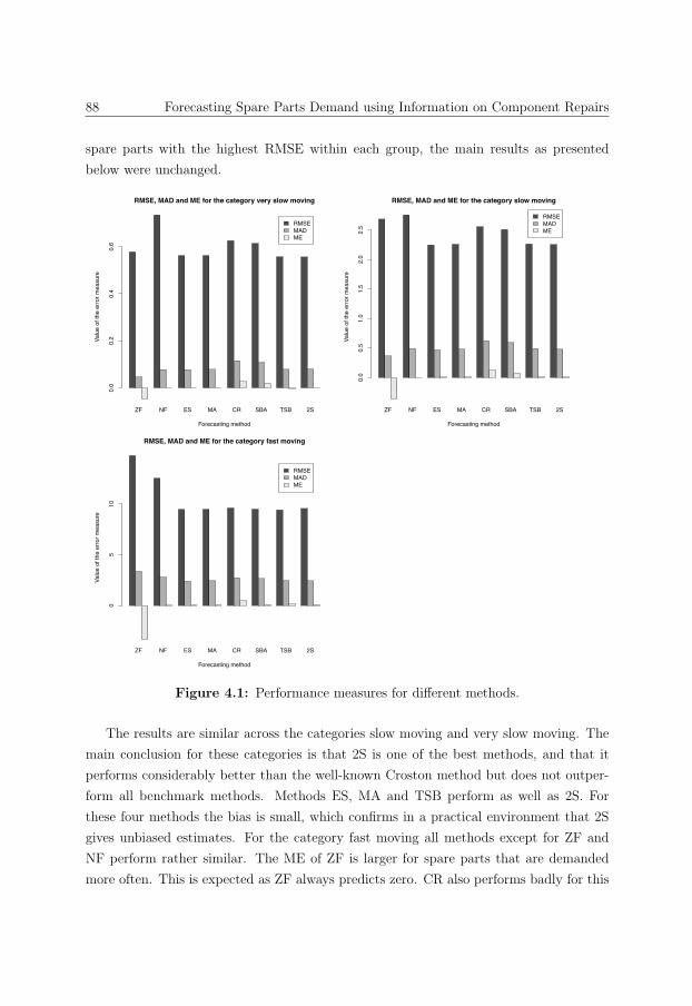
88 Forecasting Spare Parts Demand using Information on Component Repairs
spare parts with the highest RMSE within each group, the main results as presented
below were unchanged.
ZF NF ES MA CR SBA TSB 2S
RMSEMADME
RMSE, MAD and ME for the category very slow moving
Forecasting method
Valu
e of
the
erro
r mea
sure
0.0
0.2
0.4
0.6
ZF NF ES MA CR SBA TSB 2S
RMSEMADME
RMSE, MAD and ME for the category slow moving
Forecasting method
Valu
e of
the
erro
r mea
sure
0.0
0.5
1.0
1.5
2.0
2.5
ZF NF ES MA CR SBA TSB 2S
RMSEMADME
RMSE, MAD and ME for the category fast moving
Forecasting method
Valu
e of
the
erro
r mea
sure
05
10
Figure 4.1: Performance measures for different methods.
The results are similar across the categories slow moving and very slow moving. The
main conclusion for these categories is that 2S is one of the best methods, and that it
performs considerably better than the well-known Croston method but does not outper-
form all benchmark methods. Methods ES, MA and TSB perform as well as 2S. For
these four methods the bias is small, which confirms in a practical environment that 2S
gives unbiased estimates. For the category fast moving all methods except for ZF and
NF perform rather similar. The ME of ZF is larger for spare parts that are demanded
more often. This is expected as ZF always predicts zero. CR also performs badly for this
4.5 Results for case study 89
data set, and in particular has a large positive bias. Part of this empirical bias can be
attributed to the fact that the method is theoretically biased, as shown by Syntetos and
Boylan (2001). However, for their correcting SBA method, a considerable positive bias
remains. A closer look at the results at the individual part level shows that this is caused
by sudden drops in demand for many parts, e.g. because certain machines (and their
components) are taken out of operation. As argued by Teunter et al. (2011) and indeed
used as a motivation for proposing the TSB method, CR cannot deal (well) with such
sudden obsolescence issues as it does not update forecasts if no demands occur, not even
after long periods without any demand. In this way, CR and SBA overestimate demand,
and this results in a positive ME as is shown in Figure 4.1. All other methods considered
adjust their forecast toward zero during periods with no demand.
Based on the observation that sudden drops in demand occur for many parts, we would
expect that adjusting the forecasting parameters such that the methods become more
responsive to changes in demand would increase the performance. However, this is not
the case, as there are also many parts that are required on a regular basis (for example
once a year) whose forecasts are worse when they are more responsive to demand. It
cannot be predicted beforehand for which parts a sudden drop in demand will occur, and
which parts will remain to be demanded on a regular basis.
A complication for 2S of this specific dataset is that most parts can be needed for the
repair of many different components, each of which typically fail seldom. The average
number of repairs per component is less than 0.3 per month, and about 25% of the
components is repaired at most once in ten years. As a result, forecasting the number of
repaired components is hard, and maybe not much easier than directly forecasting demand
for parts. To analyze the effect of mis-estimating the numbers of repaired components on
the accuracy of the 2S method, we adjust the method by assuming that those numbers are
known. We remark that this has practical relevance for Fokker Services and in general,
as a change from a corrective to a preventive maintenance strategy would make such type
of information available, although we admit that a fraction of repairs will always remain
unplanned. For Fokker Services, it turns out that perfect foreknowledge of the number of
component to be repaired, offers little advantage for very slow moving parts but reduces
both the MAD and MSE by about 20% for slow moving as well as (relatively) fast moving
parts.
To summarize the empirical results, 2S is among a group of best performing methods
without advanced information on maintenance operations, and has the potential to consid-
erably outperform all other methods if such information is available. In the next section,
90 Forecasting Spare Parts Demand using Information on Component Repairs
we obtain further theoretical insights into the performance of 2S by studying under what
conditions it outperforms the traditional simple exponential smoothing method.
4.6 General results
As argued in Section 4.4, a benefit of 2S is that it can distinguish whether changes in
demand intensity for a part are related to changes in the demand for (certain) components
or changes in the number of parts needed per repair of a component. In this section, we will
analyze this benefit by developing a specific model for the number of repaired components
and for the number of parts needed per repair of a component. We assume that the part
(under consideration) is used to repair a single component, but will indicate at the end
of the section how the results carry over to the situation where a part type is used in the
repair of multiple components. We remark that, as we consider the single components
case, we do not use the index c throughout this section.
We consider a discrete-time model of 100 periods, i.e., t = 1, . . . , 100. Let at denote
the average demand per repair, and zt the number of repairs. For simplicity we model at
and zt as continuous random variables. We assume that
at = (μa + bt+ εt)+, (4.9)
and
zt = (μz + dt+ ηt)+, (4.10)
where εt and ηt are independently distributed with εt ∼ N(0, σ2ε ) and ηt ∼ N(0, σ2
η), and
(y)+ = max{0, y}. The demand in period t can be calculated using
dt = atzt. (4.11)
Note that both the failure rate of components and the number of parts needed to
repair are stochastic in this model, as we know from Section 4.4 that 2S and ES perform
equally well if either is constant. In the remainder of this section, we will first obtain
analytical results on the comparative performance of 2S and ES for the special case that
b = d = 0, i.e. for stationary demand, and then obtain numerical results for the general
case. For both the special and general case, we assume that forecasts are accurate at the
start (x0 = μaμz for ES; a0 = μa and z0 = μz for 2S) and analyze the accuracy in the
long run. This is without loss of generality, as initial forecast values will have a negligible
effect in the long run.
4.6 General results 91
4.6.1 Stationary demand: analytical results
Consider the situation that b = d = 0, i.e. there are no trends in either the number of
components repairs or the number of parts needed per repair. Assume that the proba-
bilities that at and zt equal zero are neglectable. We realize that this assumption is not
in line with the typical intermittence of spare parts demand, and will drop it in the next
subsection where we discuss the general case. However, it is needed to obtain analytical
insights in this subsection.
For ES we have
Cov(ε1, ε1η1) = E[ε1ε1η1]− E[ε1]E[ε1η1]
= E[ε21]E[η1]− E[ε1]2E[η1]
= 0,
and therefore
var(xES1 ) = var {(1− α)x0 + αd1}
= var {(1− α)μaμz + αa1z1}= var {α(μa + ε1)(μz + η1)}= α2var {μaμz + ε1μz + μaη1 + ε1η1}= α2 {var(ε1μz) + var(μaη1) + var(ε1η1)}= α2
{μ2zvar(ε1) + μ2
avar(η1) + E[(ε1η1)
2]− [E(ε1η1)]
2}
= α2{μ2zσ
2ε + μ2
aσ2η + E(ε1)
2E(η1)2 − [E(ε1)]
2[E(η1)]2}
= α2{μ2zσ
2ε + μ2
aσ2η + σ2
εσ2η
}.
For 2S we have
var(x2S1 ) = var {[(1− α)a0 + αa1][(1− α)z0 + αz1]}
= var {[(1− α)μa + α(μa + ε1)][(1− α)μz + α(μz + η1)]}= var {[μa + αε1][μz + αη1]}= var
{μaμz + αε1μz + αμaη1 + α2ε1η1
}={var(αε1μz) + var(αμaη1) + var(α2ε1η1)
}={α2μ2
zvar(ε1) + α2μ2avar(η1) + α4var(ε1η1)
}= α2
{μ2zσ
2ε + μ2
aσ2η + α2σ2
εσ2η
}.
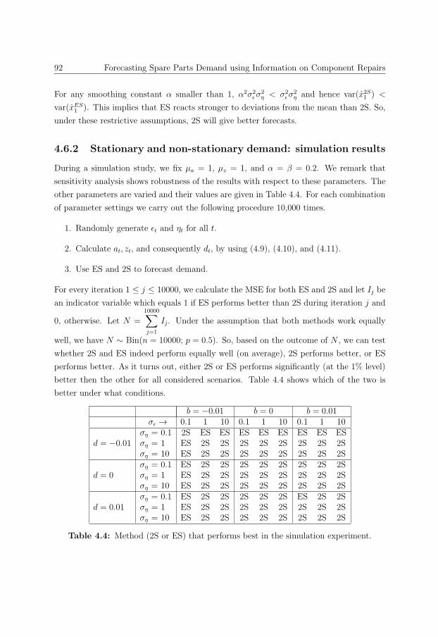
92 Forecasting Spare Parts Demand using Information on Component Repairs
For any smoothing constant α smaller than 1, α2σ2εσ
2η < σ2
εσ2η and hence var(x2S
1 ) <
var(xES1 ). This implies that ES reacts stronger to deviations from the mean than 2S. So,
under these restrictive assumptions, 2S will give better forecasts.
4.6.2 Stationary and non-stationary demand: simulation results
During a simulation study, we fix μa = 1, μz = 1, and α = β = 0.2. We remark that
sensitivity analysis shows robustness of the results with respect to these parameters. The
other parameters are varied and their values are given in Table 4.4. For each combination
of parameter settings we carry out the following procedure 10,000 times.
1. Randomly generate εt and ηt for all t.
2. Calculate at, zt, and consequently dt, by using (4.9), (4.10), and (4.11).
3. Use ES and 2S to forecast demand.
For every iteration 1 ≤ j ≤ 10000, we calculate the MSE for both ES and 2S and let Ij be
an indicator variable which equals 1 if ES performs better than 2S during iteration j and
0, otherwise. Let N =10000∑j=1
Ij. Under the assumption that both methods work equally
well, we have N ∼ Bin(n = 10000; p = 0.5). So, based on the outcome of N , we can test
whether 2S and ES indeed perform equally well (on average), 2S performs better, or ES
performs better. As it turns out, either 2S or ES performs significantly (at the 1% level)
better then the other for all considered scenarios. Table 4.4 shows which of the two is
better under what conditions.
b = −0.01 b = 0 b = 0.01σε → 0.1 1 10 0.1 1 10 0.1 1 10
ση = 0.1 2S ES ES ES ES ES ES ES ESd = −0.01 ση = 1 ES 2S 2S 2S 2S 2S 2S 2S 2S
ση = 10 ES 2S 2S 2S 2S 2S 2S 2S 2Sση = 0.1 ES 2S 2S 2S 2S 2S 2S 2S 2S
d = 0 ση = 1 ES 2S 2S 2S 2S 2S 2S 2S 2Sση = 10 ES 2S 2S 2S 2S 2S 2S 2S 2Sση = 0.1 ES 2S 2S 2S 2S 2S ES 2S 2S
d = 0.01 ση = 1 ES 2S 2S 2S 2S 2S 2S 2S 2Sση = 10 ES 2S 2S 2S 2S 2S 2S 2S 2S
Table 4.4: Method (2S or ES) that performs best in the simulation experiment.
4.7 Conclusions 93
Note that for b = 0, d = 0, 2S outperforms ES, as expected based on the analytical results
of Section 4.6.1. Table 4.4 shows that, with one exception, 2S outperforms ES unless
d = −0.01, ση = 0.1, i.e., the number of repairs is regularly decreasing over time, or
b = −0.01, σε = 0.1, i.e., the average demand per repair is regularly decreasing over time.
Interestingly, 2S works better when both trends are combined. In connection with the
case study performed for Fokker Services, the presence of obsolescence might be one of
the reasons why 2S does not outperform the benchmark methods, since this corresponds
to the situation d = −0.01 or b = −0.01. However, the negative effect of obsolescence is
not as large as for Croston’s method, since 2S is updated in every period.
For the above discussed experiment, we assumed that the spare part is used to repair
one single type of component. In addition we studied the situation where the part is used
to repair two types of components, and used (4.9), (4.10), and (4.11) to calculate demand
for each type of component. Different random numbers were used for the different types
of components. Using the same parameters as in Table 4.4 we obtained similar results.
Therefore, we expect that the conclusions from our simulation study are valid in general,
when a particular type of spare part is used to repair multiple types of components.
4.7 Conclusions
Maintaining sufficient stocks of spare parts in order to quickly carry out repair operations
is essential for service organizations. Stocking decisions should, of course, be based on de-
mand forecasts for the different part types. Existing forecasting techniques, both general
and specifically designed for slow moving demand, all base the forecasts directly on the
demand history at the part level. By doing so, they ignore the underlying process of repair
operations that explains (in part) the typical intermittent, lumpy nature of spare parts
demand. There is no demand for a part of a certain type unless a component containing
such parts is repaired (intermittency), and multiple parts may be needed to complete a
repair (lumpiness).
In this study, a forecasting method was proposed that considers the underlying repair
process. This two step (2S) method first forecasts the number of repaired components
and the number of parts per component repair (using exponential smoothing), and then
combines these into a forecast at the part level. Some analytical results were derived
that show the benefit of 2S over simple exponential smoothing (ES) in situations with
stationary demand. However, 2S did not outperform ES in an extensive empirical study
based on ten years of repair operations at Fokker Services. This can be attributed to
several causes. First, demand at the component level is also intermittent and hard to
94 Forecasting Spare Parts Demand using Information on Component Repairs
forecast. Second, most parts are contained in many different components, and hence
there is the risk of compounding forecasts errors with 2S. Third, many parts show (sudden)
drops in demand and (as shown further in a small simulation study) ES outperforms 2S
in such cases.
On the positive side, in our comparative empirical study, 2S was the joint ‘winner’
with ES, moving average (MA) and a method (TSB) that was recently proposed by Te-
unter et al. (2011); and it clearly outperforms the well-known Croston (CR) method and
(to a lesser degree) the Syntetos-Boylan (SBA) modification. Furthermore, we showed
that additional information on when components are repaired (from planned mainte-
nance/overhaul operations) may reduce the inaccuracy of 2S by up to 20%, while other
methods are not able to incorporate this information. Linking parts demand to specific
repair operations, as 2S does, also provides additional information that is important when
making inventory decisions. At Fokker Services, for instance, certain components are more
critical than others, and stocking decisions for a part could depend on how likely it is that
the part is needed for the repair of critical components.
Our study has also shown the first empirical evidence that CR and SBA cannot deal
well with sudden drops in demand, and that alternative methods such as TSB may be
less biased and more accurate if sudden obsolescence is an issue. This leads to one
interesting avenue for further research, which is to modify the 2S method so that it can
better deal with obsolescence. Other important directions for future research is to do more
empirical, comparative studies, and to obtain more analytical results on whether 2S or ES
performs best (for example in the case where a spare part is required for multiple correlated
components). Based on our empirical testing in combination with the analytical finds,
2S certainly has potential for improving forecasting accuracy for spare parts demand, but
further (empirical) research should reveal whether that potential is sufficient to overcome
the additional data collection effort.
Chapter 5
Spare parts stock control for
redundant systems using reliability
centered maintenance data
In the classical approach to determine how many spare parts to stock, the spare parts
shortage costs or the minimum fill rate are a key factor. A difficulty with this approach
lies in the estimation of these shortage costs or the determination of appropriate minimum
fill rates. In an attempt to overcome this problem, we propose to use the data gathered in
reliability centered maintenance (RCM) studies to determine shortage costs. We discuss
the benefits of this approach. At the same time, the approach gives rise to complications,
as the RCM study determines downtime costs of the underlying equipment, which have a
complex relation with the shortage cost for spare parts in case multiple pieces of equipment
have different downtime costs. A further complication is redundancy in the equipment.
We develop a framework that enables the modeling of these more complicated systems.
Based on the framework, we propose an approximative, analytic method that can be used
to determine minimum stock quantities in case of redundancy and multiple systems. In
a quantitative study we show that the method performs well. Moreover, we show that
including redundancy information in the stocking decision gives significant cost benefits.
5.1 Introduction
Availability of spare parts is important for companies, because spares are needed for
efficient operation of capital goods. When equipment breaks down, the downtime can
be significantly reduced if all spares needed for the repair are immediately available. If
96 Spare parts stock control for redundant systems using RCM data
on the other hand spares are not immediately available, the waiting time for the spares
can cause costly production losses. Because the costs of keeping spare parts on stock
can be high, it is not obvious whether we should keep stock - either how many - to
avoid downtime, or whether we should refrain from keeping stock to avoid holding costs.
It is apparent from overviews of spare parts inventory control (Rustenburg et al., 2001;
Kennedy et al., 2002) that most models aiming to support inventory decisions assume
that certain pieces of information regarding the spare parts are available. Such pieces
of information include the price and leadtime of the spare part, the usage frequency of
the part, and the shortage costs that are incurred during the waiting time for the part.
Especially the shortage costs and, in cases without demand history, the usage frequency,
are hard to estimate in practice. A method to circumvent the former problem is the
setting of so-called service level targets, but finding appropriate values for these targets
may prove difficult as well.
The research we report on was performed at a large petrochemical company. When
determining stock quantities, obtaining reasonable estimates for the shortage costs was
troublesome because of lacking data.
The company carries out reliability centered maintenance studies in order to improve
maintenance practice at their plants. Reliability centered maintenance is a structured
approach to ensure that all available data and knowledge is used to arrive at an optimal
maintenance regime (Moubray, 1991). As part of the particular type of RCM study
carried out by the company, the production loss incurred during equipment downtime,
and the estimated frequency of occurrence of different failure modes are quantitatively
determined. This data can be valuable to enhance inventory control, because the shortage
costs for spare parts are clearly related to the downtime costs of the equipment.
While in inventory models often shortage costs consisting of a single number are as-
sumed, in practice all equipment in which the spare part is used is a potential source of
downtime costs. The downtime costs of similar pieces of equipment installed in differ-
ent systems need not be equal. Another complication that came forward is redundancy.
When there are two pieces of equipment, of which only one is needed to keep the plant
running, a breakdown of one does not necessarily have severe economic consequences. In
summary, the downtime costs cannot be trivially translated to shortage costs for the spare
parts.
We contribute by proposing a new, versatile inventory model that can be used to tackle
the above-mentioned complications resulting from the use of RCM data in inventory
control. While the use of RCM data for spare part inventory control has to our best
5.1 Introduction 97
knowledge not been described in literature before, there are a number of contributions on
spare parts inventory control for redundant systems.
De Smidt-Destombes et al. (2004) investigate the trade-off between repair capacity
and spare part inventory control for a single k out of N system under condition based
maintenance; i.e. when the number of defect pieces of equipment exceeds some previously
defined limit, maintenance is initiated. They propose exact and approximate methods to
analyse the system availability. De Smidt-Destombes et al. (2006) include the possibility
that pieces of equipment degrade before failing, which complicates the analysis signifi-
cantly and allows for more refined policies. De Smidt-Destombes et al. (2007) consider
M identical k out of N systems under block replacement. For each system all defect
pieces of equipment are replaced every fixed time interval. Two methods are proposed to
analyse the system availability as a function of the number of spare parts stocked and the
block replacement interval. De Smidt-Destombes et al. (2009) consider the optimization
of the control parameters in the models presented earlier (De Smidt-Destombes et al.,
2004, 2006, 2007) to reach the target availability at minimal cost. Chakravarthy and
Gomez-Corral (2009) consider a single k out of N system, spare pieces of equipment, and
a single repair man. When a piece of equipment fails, a spare part is requested with
a given probability. A matrix analytic approach is used to evaluate the performance of
these systems.
Our model differs significantly from the models mentioned above, and none is more
general. The differences between the models result from a difference in application. In
the application examples given for the studies by De Smidt-Destombes et al., initiating
maintenance involves a major setup cost and a significant setup time, elements that
are both incorporated in their model. Neither a setup cost nor a setup time play a
significant role for our application, and these were consequently not included in our model.
Conversely, while the contributions mentioned above only consider a single system (De
Smidt-Destombes et al., 2004, 2006; Chakravarthy and Gmez-Corral, 2009) or multiple
identical systems (De Smidt-Destombes et al., 2007, 2009) , our model is very flexible in
the sense that it allows an arbitrary combination of redundant systems, between which
both the failure rate and the amount of redundancy may vary. The flexibility is needed to
make the model applicable because practical cases may involve combinations of redundant
systems with different redundancy levels and failure rates. Finally, our model is specifically
designed to work with a detailed cost structure. It is therefore possible to model a system
in which the throughput depends on the number of defect pieces of equipment in a gradual
manner, another feature that is needed to make the model applicable for use with data
coming from an RCM study.

98 Spare parts stock control for redundant systems using RCM data
Redundant systems play an important role in this research. Allocating redundancy
during the design of systems is a well-studied problem, often referred to as the redun-
dancy optimization problem (ROP). A number of variants have been studied, for a recent
overview we refer the reader to Kuo and Wan (2007). We will review contributions that
explicitly consider spare parts.
Nourelfath and Dutuit (2004) study a variant with limited repair resources (e.g. re-
pairmen/ spare parts), which are shared over all subsystems. Both this model and the
model we propose are in a sense multi-state systems, a difference being that in their model
the reliability is included via the loss of load probability (LOLP), while we include the
notion of reliability as state-dependent downtime costs. The LOLP is a meaningful and
widely-used measure of reliability during the design of systems. However, we will see
that the latter approach is more suitable to optimize spare part inventory based on RCM
data. Nourelfath and Dutuit propose a combination of the universal moment generating
function in a genetic algorithm (GA) to find a good configuration for the system with
infinite resources. This solution is used as a starting point to find a solution of the system
with finite resources, which is found heuristically based on simulation.
Nourelfath and Ait-Kadi (2007) study the same problem, except that they assume
dedicated resources for each subsystem. For this case, the process of the different sub-
systems is no longer coupled by the resource. Based on this observation, they propose
an analytic calculation of the downtime costs to replace the time consuming simulation
(Nourelfath and Dutuit, 2004). This approach is not usable in our setting, because spare
parts are often shared across subsystems.
Cantoni et al. (2000) consider the problem of optimizing the number of spare parts
for redundant systems. Marseguerra et al. (2005) extend this work to a multi criteria
approach, using the notion of pareto-dominance. The solution methodology proposed in
these works is based on a GA, and simulation is used to estimate the quality of solutions.
They propose a so called drop-by-drop approach to reduce the computational burden of
simulation, a method that was later improved by Li and Li (2010).
The use of simulation in these contributions allows for the use of a very detailed system
model. It is argued (Cantoni et al., 2000; Marseguerra et al., 2005) that, for cases with
significant safety implications, such a detailed system model is in order. We concur with
this view. Our focus will be on systems with less consequential (but still very costly)
failures. As we will argue in Section 5.2.2, for such systems, a detailed system model is
not cost effective, and a model that focuses on the most important aspects of the problem
is more suitable. Moreover, computation time is a more important issue for such systems,
implying that simulation is not the most appropriate optimization tool.

5.1 Introduction 99
Based on the knowledge that a complex system model is not cost effective for the type
of applications on which we focus, we propose a model for which the data requirements
are more limited. The model still captures the most important problem aspects, such as
redundancy and partial throughput.
To optimize the base stock level based on the model, we propose two analytic approx-
imations of the downtime costs. We develop an algorithm that can be used to determine
the optimal base stock levels based on these approximative methods. In a numerical ex-
periment, we show that the cost increase as a result of using one of the approximations
is very small, and the cost increase of the other approximation is slightly larger, but this
approximation is more intuitive to grasp. Both algorithms give results instantaneously,
and additionally are considerably easier to implement than a simulation optimization
approach.
Finkelstein (2009) also considers spare parts for redundant systems, but only non-
repairable systems are considered. A situation with a number of pieces of equipment in
series is considered, each with spare equipment in cold standby. As the number of pieces
of equipment in series goes to infinity, and under the assumption that the spares can be
shared, it is proven that the survival function of the system converges to the step function.
This result is extended to continuous resource sharing. Finally, results related to optimal
switching are derived.
Another related work is the paper by Dekker and Plasmeijer (1997). They advocate
setting quantitative estimates for unit downtime costs in complex systems in order to
facilitate decision making both on maintenance and on spare parts inventory levels. They
provide methods to estimate these downtime costs. We take a different perspective. We
will not estimate the downtime costs of individual pieces of equipment but instead directly
estimate the shortage costs of spares in the combined system.
As mentioned, one of our contributions lies in proposing a new inventory model capable
to work with RCM data. We develop fast and accurate methods to find good base stock
levels using the model. Finally, we present quantitative evidence that the value of using
the detailed RCM data is significant. In particular, we compare the costs of the proposed
methods with the costs of more traditional methods, and find significant cost benefits of
the former over the latter.
The remainder of this chapter is organized as follows. In Section 5.2 we give a de-
scription of the type of RCM study carried out at the company. We also discuss the
requirements of the model in terms of functionality and applicability. In Section 5.3 we
give a formal description of the model. We discuss the practical issues that were taken
into consideration when designing the model. In Section 5.4 methods are proposed to
100 Spare parts stock control for redundant systems using RCM data
approximate the downtime costs using the model. In Section 5.5 we describe the setup of
a numerical study based on simulation. In Section 5.6 we give the results of this study,
including investigations of the quality of the approximation and the benefits of using re-
dundancy information over more traditional approaches. In the last section, we formulate
conclusions.
5.2 Problem setting
5.2.1 The RCM data
The RCM study carried out by the company at which the research was performed is
quantitatively oriented. This makes this type of RCM study particularly valuable for
inventory control, because numerical estimates are needed in order to compare costs in
a model. The focus of a study is the critical equipment at a refinery or oil production
platform. During a study, data is gathered about this equipment. One aspect that comes
forward from a study is redundancy: the study identifies groups of pieces of equipment
that work together involving redundancy. For a group of pieces of equipment, the RCM
study gives a quantitative estimate of the cost rate that is incurred when any number of
pieces of equipment that belong to the group are defect simultaneously. This cost rate may
depend on the number of defect pieces of equipment in a gradual manner. For instance, if
out of a group of two pumps that work together, one pump is defect, partial throughput
may still be achieved resulting in a production loss of 20% (e.g. 10k$/day), while a
simultaneous breakdown of both pumps results in total production loss (50k$/day).
The study also gathers information regarding the different failure modes of the equip-
ment. For each failure mode and each group of equipment, an estimate is made of the
mean time between failure for that failure mode. When spare parts are in scope of the
study, the RCM team determines the spare part that will likely be needed when a piece
of equipment fails according to a certain failure mode. In addition, an estimate is given
of the amount of time needed to restore the system when it fails according to a certain
failure mode, under the assumption that all needed spare parts are available.
The data gathered during the study is entered into a program especially designed for
this purpose. The data is stored in structured tables, which simplifies the task of porting
this data to a decision support system for inventory control.
We conclude that the RCM data is well-structured and delivered by a team with a
lot of knowledge of the equipment. Therefore, integrating RCM data in inventory control
gives opportunities for cost effectively improving the inventory decisions.
5.2 Problem setting 101
5.2.2 Model requirements
The model we develop should enable the use of data coming from the RCM study for the
purpose of inventory control. Not all data coming from the RCM study needs to be used.
Aspects for which the added value of including them does not outweigh the decreased
usability of the model because of the increase in complexity, should be excluded. The
primary reason to refrain from using complex models is the increased burden they put on
the data collection.
The balance between realism and applicability evidently depends on the specific ap-
plication. For specific, very costly equipment with huge downtime costs (≥ $106/day),
or with critical safety functions, constructing and simulating a detailed system model
(Nourelfath and Dutuit, 2004; Cantoni et al., 2000; Marseguerra et al., 2005; Li and Li,
2010) may be a cost-effective approach to determine appropriate stock quantities for very
expensive spares (≥ $105).
We focus on spare parts with somewhat lower, but still considerable, costs, and high
downtime costs. The cases considered in Section 5.5.2 give a good picture of the type of
the applications for which the model was developed. In a single RCM study, hundreds to
thousands of such pieces of equipment may be considered. Because of the large number of
parts, and the fact that the cost of the part and of possible consequences is only moderately
high, we should limit the effort required to find an appropriate stock quantity for each
part, because spending a lot of time on this decision will not be cost effective. Therefore,
the decision making process for these parts should be (semi-) automatic, which explains
why many companies use heuristics such as the ones described in Section 5.4.4 for these
parts. As argued in the previous section, RCM is an appropriate candidate to provide
data to improve on these heuristics. However, in order to keep the model applicable, we
need to keep it simple enough such that it is practical to apply it for large numbers of
parts, without the need of a lot of additional data collection. At the same time, we must
of course make sure that sufficient characteristics are included to ensure that we improve
significantly on the simple heuristics. In the next section, we will develop a model suitable
for this purpose.
To apply this model, we need a method to determine a good base stock level for given
model parameters. For the cases on which we focus, a stock analyst will need to use this
method to enhance decision making frequently. Long computation times will hamper his
work-flow, and decrease his ability to use the system.
For this reason, it is important that the method is fast, preferably instantaneous.
While the drop-by-drop method (Cantoni et al., 2000; Marseguerra et al., 2005) is re-
ported to greatly improve the speed of simulation optimization, even an improved version
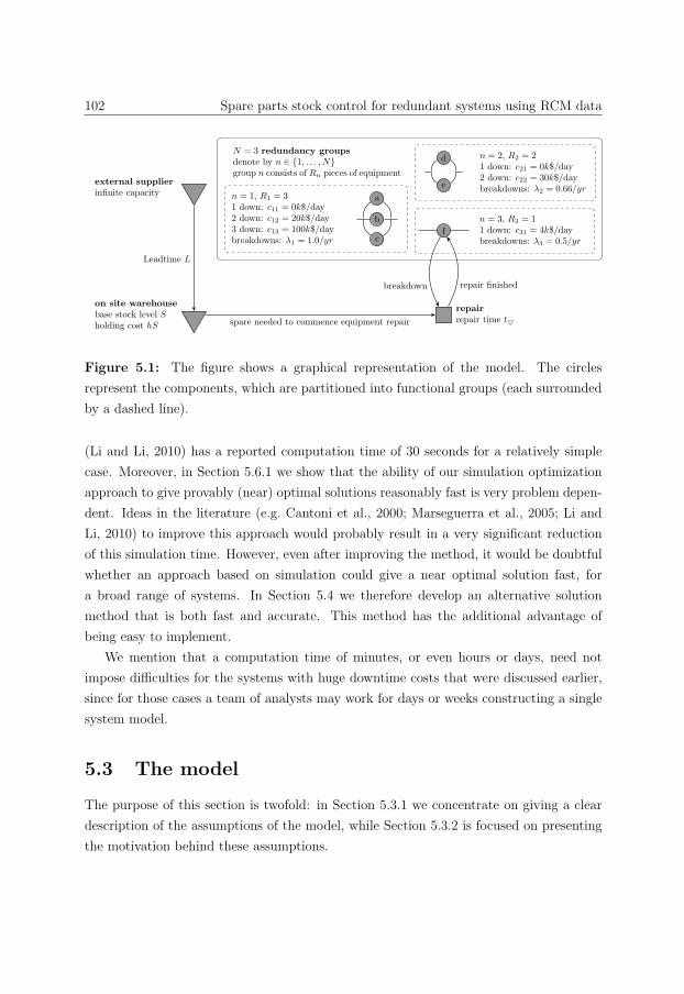
102 Spare parts stock control for redundant systems using RCM data
f
n = 3, R3 = 11 down: c31 = 4k$/daybreakdowns: λ3 = 0.5/yr
e
d n = 2, R2 = 21 down: c21 = 0k$/day2 down: c22 = 30k$/daybreakdowns: λ2 = 0.66/yr
a
b
c
n = 1, R1 = 31 down: c11 = 0k$/day2 down: c12 = 20k$/day3 down: c13 = 100k$/daybreakdowns: λ1 = 1.0/yr
N = 3 redundancy groupsdenote by n ∈ {1, . . . , N}group n consists of Rn pieces of equipment
Leadtime L
on site warehousebase stock level Sholding cost hS
external supplierinfinite capacity
spare needed to commence equipment repair
breakdown repair finished
repairrepair time t�
Figure 5.1: The figure shows a graphical representation of the model. The circles
represent the components, which are partitioned into functional groups (each surrounded
by a dashed line).
(Li and Li, 2010) has a reported computation time of 30 seconds for a relatively simple
case. Moreover, in Section 5.6.1 we show that the ability of our simulation optimization
approach to give provably (near) optimal solutions reasonably fast is very problem depen-
dent. Ideas in the literature (e.g. Cantoni et al., 2000; Marseguerra et al., 2005; Li and
Li, 2010) to improve this approach would probably result in a very significant reduction
of this simulation time. However, even after improving the method, it would be doubtful
whether an approach based on simulation could give a near optimal solution fast, for
a broad range of systems. In Section 5.4 we therefore develop an alternative solution
method that is both fast and accurate. This method has the additional advantage of
being easy to implement.
We mention that a computation time of minutes, or even hours or days, need not
impose difficulties for the systems with huge downtime costs that were discussed earlier,
since for those cases a team of analysts may work for days or weeks constructing a single
system model.
5.3 The model
The purpose of this section is twofold: in Section 5.3.1 we concentrate on giving a clear
description of the assumptions of the model, while Section 5.3.2 is focused on presenting
the motivation behind these assumptions.
5.3 The model 103
5.3.1 Formal description
We consider inventory control for a single spare part. The part is used in the repair of
multiple pieces of equipment. The model is based on the following assumptions:
1. A number of pieces of equipment are partitioned into functional groups n, where
n ∈ {1, . . . , N}. The number of pieces of equipment in group n is denoted by Rn.
2. Pieces of equipment in a redundancy group are either up (working) or down (not
working). When i out of the Rn pieces of equipment in group n are down, costs cni
per unit of time are incurred.
3. In each functional group n, as long as some of the pieces of equipment in the group
are up, breakdowns occur causing a single piece of equipment to go down. The
total breakdown rate in group n is denoted by λn. The probability of a breakdown
occurring in the group does thus not depend on the number of pieces of equipment
that are up, as long as at least one piece of equipment is up.
4. Pieces of equipment that go down can be repaired. To commence a repair a single
spare part is needed. If available, a part is immediately assigned to repair a piece
of equipment when it goes down. Otherwise it is back ordered.
5. After the spare part is available, the repair commences immediately. A deterministic
time t is needed in order to complete the repair. After the repair is completed,
the piece of equipment is considered to be up again.
6. The stock of the spare part is controlled by a continuous review base stock policy.
Under such policy the part is ordered every time it is withdrawn from stock or
back ordered, such that the total number of parts on stock and on order minus the
number of back-orders is kept equal to the base stock level S (see e.g. Axsater, 2006,
pp. 49-50). Back ordered parts are assigned on a first come first serve basis.
7. Leadtime for the part is deterministic, and denoted by L. The holding costs for
using a base stock level S are given by hS per year, where h is the annual holding
cost.
8. The system is evaluated based on the long term expected costs.
A graphical representation, along with some example parameter values, is shown in Fig-
ure 5.1. The pieces of equipment in the same functional group are depicted in a linked
structure. This is done in order to emphasize that there is redundancy involved among
104 Spare parts stock control for redundant systems using RCM data
the pieces of equipment in each group, but it should not be confused to mean that the
pieces of equipment are fully redundant.
5.3.2 Motivation
The motivation for the assumptions that constitute the model is based on the requirements
set out in Section 5.2.2.
The cost structure inherent in assumption 2 allows us to model partial throughput.
The costs are estimated in the RCM study. Note that we are interested in the marginal
costs of having a unit of extra downtime, the fixed repair costs should be excluded from
cni since they are not affected by the number of spares. The assumption of marginal
downtime costs linear in the downtime need not always hold. In some cases, the downtime
cost may depend non-linearly on the downtime interval because of pipeline capacity. This
possibility is ignored to reduce the burden of data collection.
Assumption 3 is a standard assumption in redundancy groups where only one piece of
equipment is running at a time: i.e. in so-called cold standby systems with one working
unit. In hot standby systems, i.e. systems in which multiple pieces of equipment are
running simultaneously, assumption 3 is not standard. Consider for instance a hot standby
system consisting of two pumps. Most literature assumes that the total breakdown rate
in this system is larger when both pumps are running with respect to a situation where
only one pump is running, and the other is down, since in the former case both pumps
can fail, while in the latter case, only the pump that is running can fail. A factor ignored
by standard theory however, is that the failure of one of the pumps may increase the
stress on the other pump, which may in turn increase the total breakdown rate. Both
these effects may occur, and it is not possible to determine the size of these effects in
a practical setting, because statistics regarding this point are not available. Since it is
hard to determine the most realistic modeling assumption for hot standby systems, we
will use assumption 3 for hot standby systems as well to enhance the applicability of the
model by simplifying the data requirements. Note that compared to standard assumption
for hot-standby systems in literature, our estimate of the downtime costs will be higher,
because in our model the failure rate in the system will not decrease as more pieces of
equipment are down. This makes our approach a more conservative approach, which is
beneficial in light of the above discussion.
Assumptions 4 and 5 imply that obtaining the spare part and repairing the equipment
commences immediately after the equipment breaks down. These assumptions do not hold
in general, as in redundant systems, a failure need not be immediately detectable. In cold
5.4 Approximate analysis 105
standby systems, a piece of equipment not running may degrade and break down, which
happens undetected until one attempts to activate the equipment. Undetected failures
are a big threat that should be mitigated by frequent testing, for instance by switching
of the running equipment. If testing is so frequent that failures are detected within a
time span much smaller than the other time scales of the problem, the applicability of
the model is not hurt by the undetected failures.
A further limitation of assumptions 4 and 5 is finite repair capacity. When a lot
of equipment fails in a short time interval, there may not be sufficient repairmen to
finish all repairs in regular working hours. Note however that the repairmen perform the
maintenance for all equipment on the site, while the spare parts are only used in a very
limited number of equipment. The relative variation in the workload of the repairmen
is thus considerably less than the relative variation in the usage of the spare parts, as
a result the capacity problem related to repairmen is relatively less costly to mitigate.
Furthermore, to finish at least the repair of the critical equipment considered in this
chapter overtime should be considered.
The assumption of a base stock policy (assumption 6 ) is motivated by the fact that
we focus on expensive spare parts. For those parts, the ordering costs are dominated by
holding costs, implying that batching in order to reduce ordering costs will not be cost
effective.
Assumption 7 prescribes that holding costs are linear in the base stock level S. This
assumption is common when holding costs are paid for parts on order as well as parts
on stock.With regard to assumption 7 we mention an important issue that needs to be
resolved in order to apply the model. Data on leadtime and cost must be obtained from the
supplier in a standard format. We will not go into details on this issue, but we mention
that a well-defined procedure to obtain reliable data on the spare parts themselves is
essential for successful inventory control. Furthermore, data must be obtained describing
which parts are used in the repair of which equipment. Even though this may not be
standardly included in an RCM study, this data can be obtained during the study. The
data can also be obtained in a separate study.
5.4 Approximate analysis
The purpose of the model presented in the previous section is the optimization of the
base stock level. As discussed in Section 5.2.2 it is important to have a fast method for
performing this optimization. In this section we will develop such a method.
106 Spare parts stock control for redundant systems using RCM data
In order to optimize the base stock level, we need to determine the downtime costs for
different values of the base stock level. Note that we will evaluate the system based on
the long term expected costs.
In Section 5.4.1 we show that under deterministic waiting times for spares, the expected
amount of downtime and the downtime costs can be easily evaluated. In Section 5.4.2 we
use this observation to propose two approximative methods for evaluating the downtime
costs for a given base stock level. In Section 5.4.3 we show how to use the approximations
to determine base stock levels. In Section 5.4.4 we present two traditional methods that
will be used to benchmark our approach, and to gain insight in the relative value of using
the more sophisticated approaches described in Sections 5.4.1-5.4.3.
5.4.1 The downtime costs for fixed total repair time
The total repair time is composed of the waiting time for spares and the remaining repair
time after spares are available (t). The waiting time for individual repairs depends on
the state of the warehouse at the moment of failure. This couples the different functional
groups, and gives the systems its complexity.
In this section, we show how to calculate the long term expected downtime costs for a
single functional group under the assumption that the waiting time for spares, and thus
the total repair time, is fixed and deterministic. While this assumption is not satisfied
in our model, the theory developed in this section will serve as a building block for the
approximations for the downtime cost of the whole system that will be presented in the
next section. We denote the fixed waiting time for spares by tw,f . The total repair time
is then also deterministic, and has length t + tw,f , which will be denoted by tf .
Note that under the assumption of fixed waiting times, the functional groups decouple.
Consider functional group n ∈ {1, . . . , N}. This functional group can be represented by
a closed queueing network with Rn customers and two stations: (i) an ample server with
mean service time tf , representing the repair process; (ii) an exponential server with mean
service time 1/λn, which represents the failure process. This network belongs to the class
of so-called BCMP networks and thus has a product-form solution (see Baskett et al.,
1975). The steady state probabilities of having i ∈ {0, . . . , Rn} defect pieces of equipment
in this functional group is thus equal to
pn(i, tf ) =
((λntf )
i
i!
)/( Rn∑j=0
(λntf )j
j!
). (5.1)
5.4 Approximate analysis 107
The long term expected downtime costs Cn for functional group n can be calculated
from the steady state probabilities given by (5.1) using the following relation
Cn(tf ) =Rn∑i=1
cnipn(i, tf ). (5.2)
The total downtime costs for a fixed repair time are the sum of the downtime costs for
the individual functional groups,
Cfixed(tf ) =N∑
n=1
Cn(tf ). (5.3)
5.4.2 Approximating the downtime costs
In the previous section we showed that under the assumption of deterministic waiting
times for spares, the downtime costs can be computed efficiently. In this section we will
present two methods to approximate the total downtime costs for the dynamic system.
For both approximations, we will approximate the total demand rate for spares by
a Poisson demand stream. We have assumed that the rate at which failures occur is
given by λn for every functional group n, as long as there is any equipment running in
that functional group. Each time a failure occurs, a spare part is needed. In practice,
downtime of equipment is short in comparison to the uptime of the equipment even in
case no spare parts are stocked. Each functional group thus gives rise to a demand stream
which can be approximated by a Poisson process with rate λn. It is thus reasonable to
approximate the total demand rate for spare parts as a Poisson process with rate
λ =N∑
n=1
λn. (5.4)
The average waiting time approximation will be based upon the average waiting time
for spares, which will be denoted by tw. It depends on the total demand rate (approxi-
mated by λ), the leadtime L, and the base stock level S. Under our approximation, the
demand in an arbitrary interval of length L is Poisson distributed, with mean λL. Let
us denote this random variable by Xp. Let us calculate the average number of parts in
108 Spare parts stock control for redundant systems using RCM data
backorder:
E(max(Xp − S, 0)) =∞∑i=S
(i− S)(λL)i
i!e−λL,
= λL− S −S−1∑i=0
(i− S)(λL)i
i!e−λL.
From this expression, the average waiting time can be calculated using Little’s formula
(1961):
tw = L− S
λ+
1
λ
S−1∑i=0
(S − i)(λL)i
i!e−λL. (5.5)
The total average expected repair time is now given by
t = tw + t. (5.6)
We will use this average in (5.3) to approximate the downtime costs:
Caverage = Cfixed(t) (5.7)
The approximation is similar to the one used in the analysis of the METRIC model, pro-
posed by Sherbrooke (1968). In Section 5.6 we will see that the approximation sometimes
performs poorly.
To improve the performance we propose a second approximation, the dynamic-static
waiting time approximation. The repair resulting from an arbitrary breakdown incurs a
stochastic delay due to the waiting time for spares, which can be zero or positive. When
the spares demand is approximated by a Poisson demand stream, a simple expression can
be derived for the distribution of this stochastic delay. We will first derive this expression.
Then we will show how to use the expression to obtain an approximation for the downtime
costs.
Consider an arbitrary breakdown, which we assume to occur at time t. Recall that
we assume a base stock policy with base stock level S is used and that stock is allocated
on a first come first served basis. Consequently, the part that was ordered when the
Sth breakdown preceding the current breakdown occurred, will be used in the repair of
the current breakdown. Say this earlier breakdown occurred at time t − X. Recall the
approximative assumption of a Poisson repair stream. Then X is Erlang-k distributed,
with k = S: it is the sum of S exponentially distributed variables with mean 1/λ. When
5.4 Approximate analysis 109
S = 0 then X = 0 with probability 1. The part arrives at time t−X + L. Therefore, at
time t the remaining waiting time is max(0, L−X). This random variable will be denoted
by Y .
Under the dynamic static waiting time approximation the expected downtime is ap-
proximated as follows:
Cdyn.-st. = E(Cfixed(Y + t)) (5.8)
where Cfixed is determined using (5.3). Note that the average waiting time approximation
differs because
Caverage = Cfixed(t) = Cfixed(E(Y ) + t)
Compared with simulation, it is relatively easy to evaluate (5.8) numerically, a number
of standard methods are available. For completeness, we describe how we evaluated the
expression in our numerical experiments. We use that
Cdyn.-st. =E(Cfixed(max(0, L−X) + t)),
=P (X > L)Cfixed(t) + P (X < L)
× E(Cfixed(L−X + t)|X < L).
Since the CDF of the Erlang distribution can be calculated analytically, the first term can
be easily calculated. The PDF of the Erlang distribution is also analytically calculable,
let us denote it by f(x). We have that
P (X < L)E(Cfixed(L−X + t)|X < L)
=
∫ L
0
f(x)Cfixed(L− x+ t)dx,
≈ 1
M
M−1∑i=0
f(i/M)Cfixed(L(1− i/M) + t).
In our numerical tests, we use M = 105.
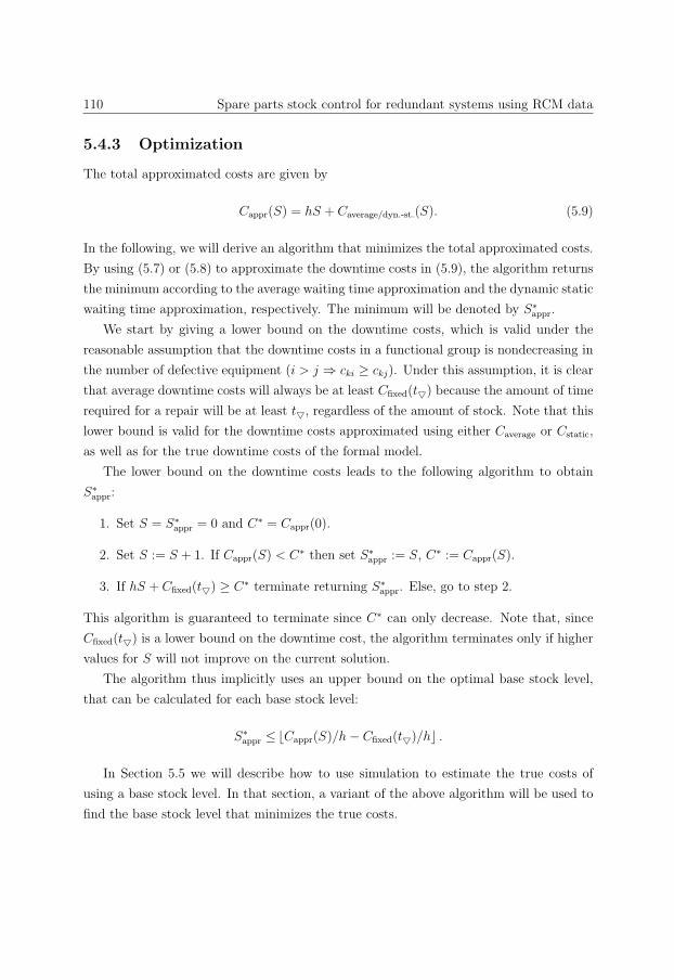
110 Spare parts stock control for redundant systems using RCM data
5.4.3 Optimization
The total approximated costs are given by
Cappr(S) = hS + Caverage/dyn.-st.(S). (5.9)
In the following, we will derive an algorithm that minimizes the total approximated costs.
By using (5.7) or (5.8) to approximate the downtime costs in (5.9), the algorithm returns
the minimum according to the average waiting time approximation and the dynamic static
waiting time approximation, respectively. The minimum will be denoted by S∗appr.
We start by giving a lower bound on the downtime costs, which is valid under the
reasonable assumption that the downtime costs in a functional group is nondecreasing in
the number of defective equipment (i > j ⇒ cki ≥ ckj). Under this assumption, it is clear
that average downtime costs will always be at least Cfixed(t) because the amount of time
required for a repair will be at least t, regardless of the amount of stock. Note that this
lower bound is valid for the downtime costs approximated using either Caverage or Cstatic,
as well as for the true downtime costs of the formal model.
The lower bound on the downtime costs leads to the following algorithm to obtain
S∗appr:
1. Set S = S∗appr = 0 and C∗ = Cappr(0).
2. Set S := S + 1. If Cappr(S) < C∗ then set S∗appr := S, C∗ := Cappr(S).
3. If hS + Cfixed(t) ≥ C∗ terminate returning S∗appr. Else, go to step 2.
This algorithm is guaranteed to terminate since C∗ can only decrease. Note that, since
Cfixed(t) is a lower bound on the downtime cost, the algorithm terminates only if higher
values for S will not improve on the current solution.
The algorithm thus implicitly uses an upper bound on the optimal base stock level,
that can be calculated for each base stock level:
S∗appr ≤�Cappr(S)/h− Cfixed(t)/h� .
In Section 5.5 we will describe how to use simulation to estimate the true costs of
using a base stock level. In that section, a variant of the above algorithm will be used to
find the base stock level that minimizes the true costs.
5.5 Setup of simulation experiment 111
5.4.4 Traditional inventory methods
We will also examine two methods for solving the problem, that will be used as a bench-
mark in the numerical experiment. The traditional methods do not take into account
detailed redundancy information, and they represent what companies might do if data
regarding redundancy is not available or if they lack the know-how or organizational
structure needed to couple the redundancy information with spare parts stock control.
The first method assumes that an estimate is used for the total demand rate (equal
to λ, as given by (5.4)) and the leadtime. The system is modeled as a base stock model
in which demand is back ordered. Then, it is easy to evaluate the fraction of parts that
are delivered from stock in the steady state of the system, a fraction often referred to as
fill rate (see e.g. Axsater, 2006, pp. 94-95).
In the method, we then use a fill rate target to determine the base stock level. The
lowest base stock level for which the target fill rate is reached is chosen. Since we assume
no additional information is available based on which the target could be varied, we
assume the same target is used for each part. To gain some insight in the sensitivity of
the method with respect to this target, we will vary it. We will denote the method that
uses a particular target fill rate by this target in quotation marks. E.g. “95%” denotes
the method that uses a fill rate target of 95% over all cases.
In the second traditional method, we assume that the highest possible downtime cost
for all pieces of equipment in which the part is installed can be determined. This downtime
costs is then used as the penalty cost per time period in the system, again modeling the
system as a Poisson demand system in which demand is back-ordered. The overall costs
(downtime + holding) are then minimized to obtain the optimal base stock level. This
method is similar to the method currently used by the company as a recommendation
to the stock analysts (Trimp et al., 2004). Note that while it has some awareness of the
downtime costs, it does not use any redundancy information. We will refer to this second
traditional method as benchmark method later on.
5.5 Setup of simulation experiment
5.5.1 Simulation
The analysis discussed in the previous section gives approximative estimates of the down-
time costs, based on which approximately optimal base stock levels can be determined.
In order to test the quality of these approximations and the resulting recommendations,
we describe in this section a simulation approach that enables us to find asymptotically
112 Spare parts stock control for redundant systems using RCM data
exact estimates of the downtime costs. We also describe the approach that was used to
find the optimal base stock level using simulation.
To avoid confusion, let us first stress that in the simulation we aim to find downtime
costs for the model described in Section 5.3. All assumptions discussed in that section
thus remain in place. Our aim is to estimate the quality of the approximations and
the traditional methods presented in Sections 5.4.2 and 5.4.4, and the quality of the
recommendations that result from using the approximations.
In order to assess the effect of these approximations, we need the true costs of the
system. To this end, we simulate the system. We use event-driven simulation. The
system is simulated for a long period of time, which is divided in batches with a length of
1000 years. We then use the standard approach to obtain asymptotically correct estimates
of the long term expected downtime costs and the associated variance.
To find the optimal base stock level using simulation, we would like to find the associ-
ated cost for all base stock levels up to some upper bound with very high precision. This,
however, turns out to be impossible for some cases. In order to obtain consistent results,
the following procedure has been developed.
We start by considering S = 0, and increment S each step. For each step, we obtain an
initial estimator of the downtime costs and its associated standard deviation, by simulating
the system until we have 1000 periods of 1000 years for which the total downtime costs are
positive. While for most systems in each 1000 year period downtime costs are incurred,
in some systems in only 1 out of more than 250 periods positive costs are found. The
described method is used to ensure that it is reasonable to apply the central limit theorem
for the estimator. We continue increasing S until both the following conditions are met:
• The current base stock level exceeds the “optimal” base stock levels calculated using
the different approximative methods described in Sections 5.4.2 and 5.4.4.
• The holding cost for the current solution plus the lower bound for the downtime
cost exceed the estimate of the total costs for the best base stock level found so far
plus five times its standard deviation (see Section 5.4.3). By including five times
the standard deviation, we ensure against cutting of the optimization prematurely.
Note that we have taken extensive measures to assure that the optimal base stock level
is included.
The relative deviation of the estimators may however be quite high at this point. In
order to decrease this variance, we continue by simulating for each base stock level until
the resulting estimator reaches a target relative deviation, which is set at 2−10 ≈ 10−3.
While we cannot guarantee that we find the true minimum in this way, we can state that
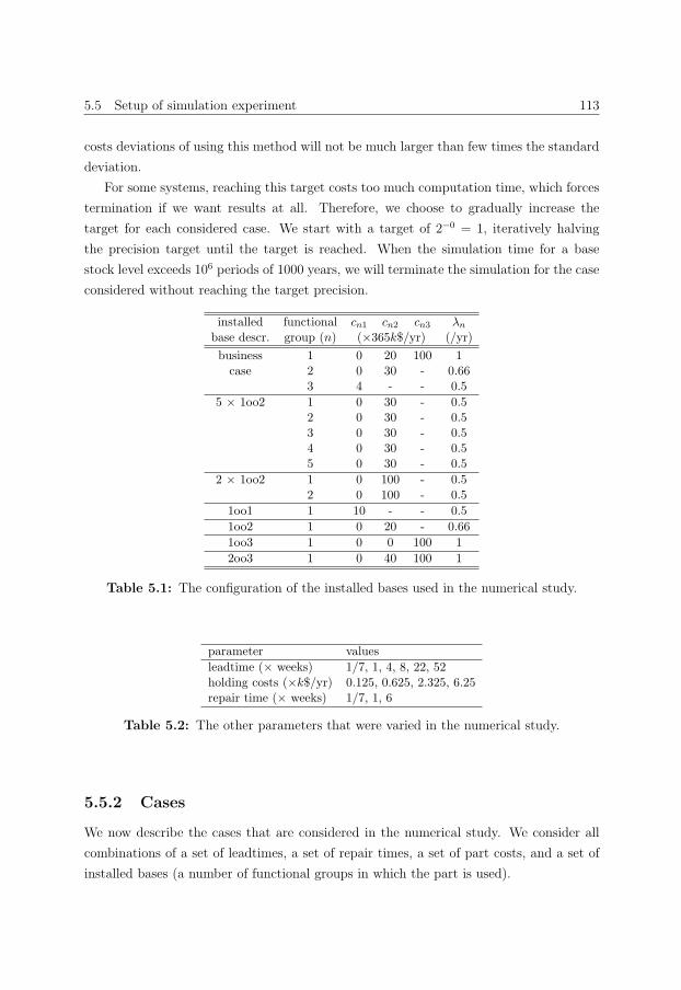
5.5 Setup of simulation experiment 113
costs deviations of using this method will not be much larger than few times the standard
deviation.
For some systems, reaching this target costs too much computation time, which forces
termination if we want results at all. Therefore, we choose to gradually increase the
target for each considered case. We start with a target of 2−0 = 1, iteratively halving
the precision target until the target is reached. When the simulation time for a base
stock level exceeds 106 periods of 1000 years, we will terminate the simulation for the case
considered without reaching the target precision.
installed functional cn1 cn2 cn3 λn
base descr. group (n) (×365k$/yr) (/yr)
business 1 0 20 100 1case 2 0 30 - 0.66
3 4 - - 0.5
5 × 1oo2 1 0 30 - 0.52 0 30 - 0.53 0 30 - 0.54 0 30 - 0.55 0 30 - 0.5
2 × 1oo2 1 0 100 - 0.52 0 100 - 0.5
1oo1 1 10 - - 0.5
1oo2 1 0 20 - 0.66
1oo3 1 0 0 100 1
2oo3 1 0 40 100 1
Table 5.1: The configuration of the installed bases used in the numerical study.
parameter values
leadtime (× weeks) 1/7, 1, 4, 8, 22, 52holding costs (×k$/yr) 0.125, 0.625, 2.325, 6.25repair time (× weeks) 1/7, 1, 6
Table 5.2: The other parameters that were varied in the numerical study.
5.5.2 Cases
We now describe the cases that are considered in the numerical study. We consider all
combinations of a set of leadtimes, a set of repair times, a set of part costs, and a set of
installed bases (a number of functional groups in which the part is used).
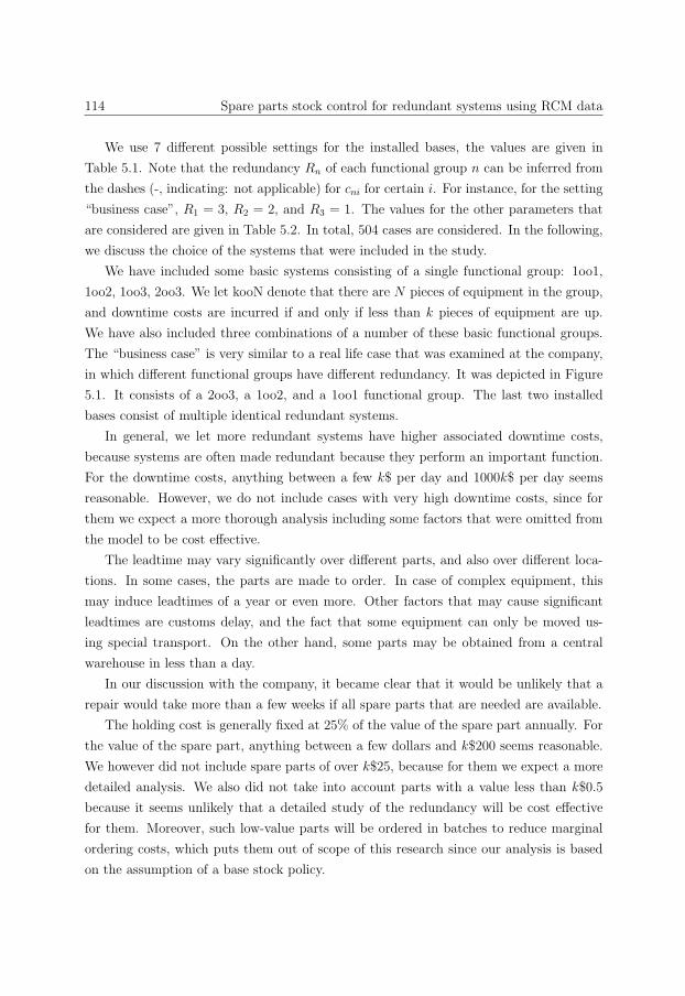
114 Spare parts stock control for redundant systems using RCM data
We use 7 different possible settings for the installed bases, the values are given in
Table 5.1. Note that the redundancy Rn of each functional group n can be inferred from
the dashes (-, indicating: not applicable) for cni for certain i. For instance, for the setting
“business case”, R1 = 3, R2 = 2, and R3 = 1. The values for the other parameters that
are considered are given in Table 5.2. In total, 504 cases are considered. In the following,
we discuss the choice of the systems that were included in the study.
We have included some basic systems consisting of a single functional group: 1oo1,
1oo2, 1oo3, 2oo3. We let kooN denote that there are N pieces of equipment in the group,
and downtime costs are incurred if and only if less than k pieces of equipment are up.
We have also included three combinations of a number of these basic functional groups.
The “business case” is very similar to a real life case that was examined at the company,
in which different functional groups have different redundancy. It was depicted in Figure
5.1. It consists of a 2oo3, a 1oo2, and a 1oo1 functional group. The last two installed
bases consist of multiple identical redundant systems.
In general, we let more redundant systems have higher associated downtime costs,
because systems are often made redundant because they perform an important function.
For the downtime costs, anything between a few k$ per day and 1000k$ per day seems
reasonable. However, we do not include cases with very high downtime costs, since for
them we expect a more thorough analysis including some factors that were omitted from
the model to be cost effective.
The leadtime may vary significantly over different parts, and also over different loca-
tions. In some cases, the parts are made to order. In case of complex equipment, this
may induce leadtimes of a year or even more. Other factors that may cause significant
leadtimes are customs delay, and the fact that some equipment can only be moved us-
ing special transport. On the other hand, some parts may be obtained from a central
warehouse in less than a day.
In our discussion with the company, it became clear that it would be unlikely that a
repair would take more than a few weeks if all spare parts that are needed are available.
The holding cost is generally fixed at 25% of the value of the spare part annually. For
the value of the spare part, anything between a few dollars and k$200 seems reasonable.
We however did not include spare parts of over k$25, because for them we expect a more
detailed analysis. We also did not take into account parts with a value less than k$0.5
because it seems unlikely that a detailed study of the redundancy will be cost effective
for them. Moreover, such low-value parts will be ordered in batches to reduce marginal
ordering costs, which puts them out of scope of this research since our analysis is based
on the assumption of a base stock policy.
5.6 Results & discussion 115
5.6 Results & discussion
The results of the numerical experiments are presented and discussed in this section.
5.6.1 Computation times
As stated before, the main reason for using approximative methods to optimize the base
stock level instead of simulation are the significant CPU times required for simulation
optimization. The required processor times for the simulation optimization of the consid-
ered cases are shown in Table 5.3. The simulations were performed on a 2.33 GHz dual
core CPU with 3.23 GB of RAM, on two separate threads running in parallel.
attained # of avg. comp. time per caseprecision cases performed for target
2−10 368 9 min -2−9 44 34 min 2 hrs2−8 40 51 min 13 hrs2−7 28 30 min 32 hrs2−6 12 28 min 482 hrs2−5 7 22 min 1478 hrs2−4 5 22 min 5882 hrs
Table 5.3: The statistics regarding the attained precision and the CPU times in the
simulation. We also tabulate an estimate of additional CPU time that would be needed
to attain the precision target.
The target precision was set at a normalized standard deviation smaller than 2−10 ≈10−3. For the cases for which the target was attained, the average simulation time was 9
minutes.
Some simulations were terminated before the target relative deviation was attained.
Statistics regarding this point are also tabulated. An estimate of the additional simulation
time that would be required to attain the target is tabulated as well, where we use that
the standard deviation of the estimator is ∼ 1/√n, where n is the number of 1000 year
periods. The table shows that while the target precision is relatively modest, attaining it
would require a prohibitive amount of effort for some cases. The reason for this is that
for some systems with redundancy and higher stocks, periods of costly downtime are rare.
For these systems, it is hard to control the variance of the estimator using simulation. For
instance, in a system in which a period with costs of k$3000 occurs every ∼ 1500 years, to
get the relative deviation below 0.1% would require simulating the system for ∼ 1.5× 10⁹
years (even without taking into account any variance in the costs of an event itself).
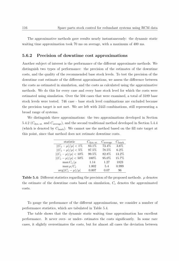
116 Spare parts stock control for redundant systems using RCM data
The approximative methods gave results nearly instantaneously: the dynamic static
waiting time approximation took 70 ms on average, with a maximum of 400 ms.
5.6.2 Precision of downtime cost approximations
Another subject of interest is the performance of the different approximate methods. We
distinguish two types of performance: the precision of the estimates of the downtime
costs, and the quality of the recommended base stock levels. To test the precision of the
downtime cost estimate of the different approximations, we assess the difference between
the costs as estimated in simulation, and the costs as calculated using the approximative
methods. We do this for every case and every base stock level for which the costs were
estimated using simulation. Over the 504 cases that were examined, a total of 3189 base
stock levels were tested. 746 case - base stock level combinations are excluded because
the precision target is not met. We are left with 2443 combinations, still representing a
broad range of systems.
We distinguish three approximations: the two approximations developed in Section
5.4.2 (Cdyn.-st. and Caverage), and the second traditional method developed in Section 5.4.4
(which is denoted by Cbmrk). We cannot use the method based on the fill rate target at
this point, since that method does not estimate downtime costs.
statistic Cdyn.-st. Caverage Cbmrk
|(Ce − μ)/μ| < 1% 83.1% 73.4% 3.6%|(Ce − μ)/μ| < 5% 97.5% 78.5% 6.2%|(Ce − μ)/μ| < 10% 99.5% 82.8% 13.2%|(Ce − μ)/μ| < 50% 100% 95.0% 15.7%
maxCe/μ 1.14 1.27 1823maxμ/Ce 1.002 5.4 0.999
avg|(Ce − μ)/μ| 0.007 0.07 96
Table 5.4: Different statistics regarding the precision of the proposed methods. μ denotes
the estimate of the downtime costs based on simulation, Ce denotes the approximated
costs.
To gauge the performance of the different approximations, we consider a number of
performance statistics, which are tabulated in Table 5.4.
The table shows that the dynamic static waiting time approximation has excellent
performance. It never over- or under- estimates the costs significantly. In some rare
cases, it slightly overestimates the costs, but for almost all cases the deviation between
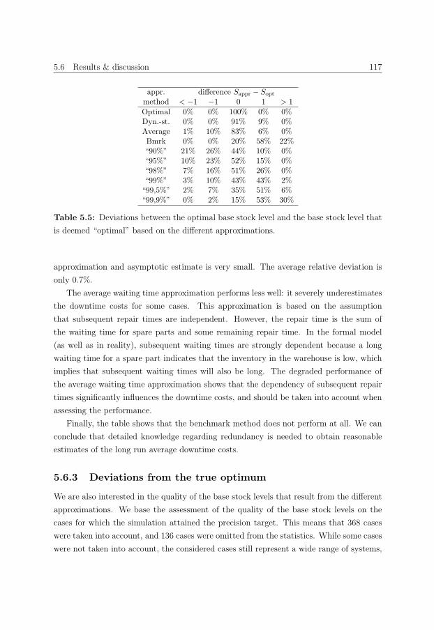
5.6 Results & discussion 117
appr. difference Sappr − Sopt
method < −1 −1 0 1 > 1
Optimal 0% 0% 100% 0% 0%Dyn.-st. 0% 0% 91% 9% 0%Average 1% 10% 83% 6% 0%Bmrk 0% 0% 20% 58% 22%“90%” 21% 26% 44% 10% 0%“95%” 10% 23% 52% 15% 0%“98%” 7% 16% 51% 26% 0%“99%” 3% 10% 43% 43% 2%“99,5%” 2% 7% 35% 51% 6%“99,9%” 0% 2% 15% 53% 30%
Table 5.5: Deviations between the optimal base stock level and the base stock level that
is deemed “optimal” based on the different approximations.
approximation and asymptotic estimate is very small. The average relative deviation is
only 0.7%.
The average waiting time approximation performs less well: it severely underestimates
the downtime costs for some cases. This approximation is based on the assumption
that subsequent repair times are independent. However, the repair time is the sum of
the waiting time for spare parts and some remaining repair time. In the formal model
(as well as in reality), subsequent waiting times are strongly dependent because a long
waiting time for a spare part indicates that the inventory in the warehouse is low, which
implies that subsequent waiting times will also be long. The degraded performance of
the average waiting time approximation shows that the dependency of subsequent repair
times significantly influences the downtime costs, and should be taken into account when
assessing the performance.
Finally, the table shows that the benchmark method does not perform at all. We can
conclude that detailed knowledge regarding redundancy is needed to obtain reasonable
estimates of the long run average downtime costs.
5.6.3 Deviations from the true optimum
We are also interested in the quality of the base stock levels that result from the different
approximations. We base the assessment of the quality of the base stock levels on the
cases for which the simulation attained the precision target. This means that 368 cases
were taken into account, and 136 cases were omitted from the statistics. While some cases
were not taken into account, the considered cases still represent a wide range of systems,
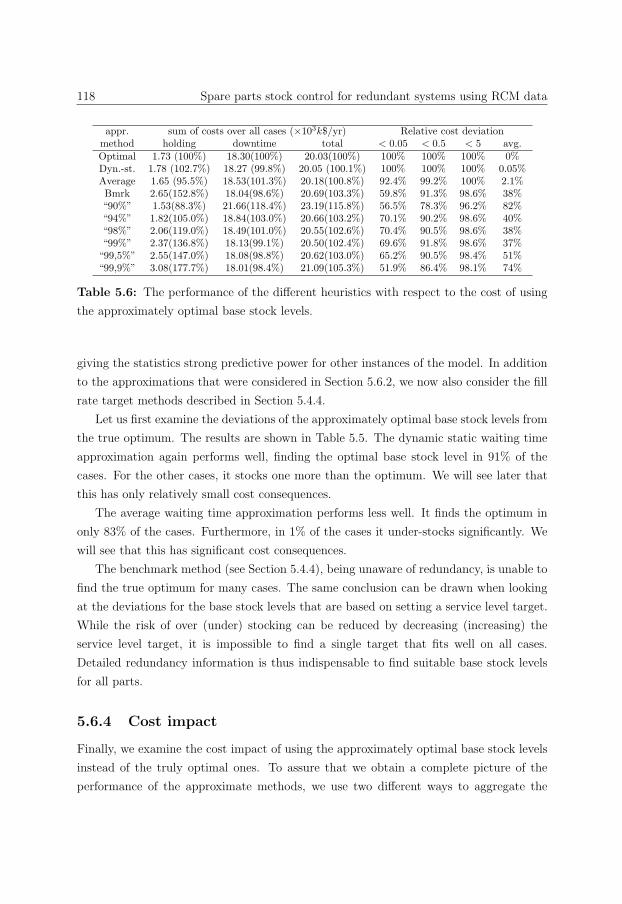
118 Spare parts stock control for redundant systems using RCM data
appr. sum of costs over all cases (×103k$/yr) Relative cost deviationmethod holding downtime total < 0.05 < 0.5 < 5 avg.Optimal 1.73 (100%) 18.30(100%) 20.03(100%) 100% 100% 100% 0%Dyn.-st. 1.78 (102.7%) 18.27 (99.8%) 20.05 (100.1%) 100% 100% 100% 0.05%Average 1.65 (95.5%) 18.53(101.3%) 20.18(100.8%) 92.4% 99.2% 100% 2.1%Bmrk 2.65(152.8%) 18.04(98.6%) 20.69(103.3%) 59.8% 91.3% 98.6% 38%“90%” 1.53(88.3%) 21.66(118.4%) 23.19(115.8%) 56.5% 78.3% 96.2% 82%“94%” 1.82(105.0%) 18.84(103.0%) 20.66(103.2%) 70.1% 90.2% 98.6% 40%“98%” 2.06(119.0%) 18.49(101.0%) 20.55(102.6%) 70.4% 90.5% 98.6% 38%“99%” 2.37(136.8%) 18.13(99.1%) 20.50(102.4%) 69.6% 91.8% 98.6% 37%“99,5%” 2.55(147.0%) 18.08(98.8%) 20.62(103.0%) 65.2% 90.5% 98.4% 51%“99,9%” 3.08(177.7%) 18.01(98.4%) 21.09(105.3%) 51.9% 86.4% 98.1% 74%
Table 5.6: The performance of the different heuristics with respect to the cost of using
the approximately optimal base stock levels.
giving the statistics strong predictive power for other instances of the model. In addition
to the approximations that were considered in Section 5.6.2, we now also consider the fill
rate target methods described in Section 5.4.4.
Let us first examine the deviations of the approximately optimal base stock levels from
the true optimum. The results are shown in Table 5.5. The dynamic static waiting time
approximation again performs well, finding the optimal base stock level in 91% of the
cases. For the other cases, it stocks one more than the optimum. We will see later that
this has only relatively small cost consequences.
The average waiting time approximation performs less well. It finds the optimum in
only 83% of the cases. Furthermore, in 1% of the cases it under-stocks significantly. We
will see that this has significant cost consequences.
The benchmark method (see Section 5.4.4), being unaware of redundancy, is unable to
find the true optimum for many cases. The same conclusion can be drawn when looking
at the deviations for the base stock levels that are based on setting a service level target.
While the risk of over (under) stocking can be reduced by decreasing (increasing) the
service level target, it is impossible to find a single target that fits well on all cases.
Detailed redundancy information is thus indispensable to find suitable base stock levels
for all parts.
5.6.4 Cost impact
Finally, we examine the cost impact of using the approximately optimal base stock levels
instead of the truly optimal ones. To assure that we obtain a complete picture of the
performance of the approximate methods, we use two different ways to aggregate the
5.6 Results & discussion 119
statistics of individual cases. First of all, we consider the real costs (as determined using
simulation) of implementing the approximately optimal base stock levels for all cases.
These costs can be interpreted as the costs of implementing a certain policy at a company,
i.e. for a diverse range of cases. Also, we gather statistics regarding the number of cases for
which the relative deviation between the optimal costs and the cost of the approximately
optimal base stock level (both costs determined using simulation) exceeds some threshold.
The results are shown in Table 5.6. The two ways to aggregate the information give a
somewhat different perspective.
Let us now first discuss the cost totals over all different cases when using the different
approximations. The dynamic static waiting time approximation performs well. In com-
parison to the optimal policy, the cost increase is 0.1%. Later on, we will argue that a
more accurate comparison is obtained when focusing more on the relative stock increase.
The dynamic static waiting time approximation uses 2.7% more stock than the optimal
solution, of which ∼ 65% is offset because of reduced downtime costs.
The average waiting time approximation has a slightly worse performance. It stocks
somewhat less than the optimal policy, but incurs severe additional downtime costs as a
result. The deteriorated performance is closely related to the fact that the average waiting
time approximation significantly underestimates the downtime costs for some cases. The
additional downtime costs are 0.23×10³k$/yr. This is about 14% of the total stock costs.
The decrease in stock cost is only 4.5% of the total stock costs, resulting in a nett cost
increase of 9.5% of the total stock cost, or 0.8% of the total cost.
Let us now discuss the other approximations. The benchmark method severely over-
stocks, but realizes some additional availability. However, this additional availability is
not realized in a cost effective manner: the overall costs increase by 3.3%. Even though
this might seem a small effect, comparing the cost increase with the total cost does not
give an accurate picture. In an organization, the downtime costs are often hidden, since
they translate to production that was not made. Moreover, a large fraction of the down-
time costs are unavoidable, because even without any stock outs, downtime costs are still
significant because of the remaining repair times. A more accurate picture of the impact
on the company performance is obtained by concentrating on the holding cost (which
are linear in the stock value). The benchmark method uses 52.8% more stock than the
optimal stock quantity. Only ∼ 28% of this 52.8% is offset by the increased availability.
This means that the benchmark method leaves huge opportunities for improvement.
Note that in order to apply the benchmark method we do not need detailed information
regarding the redundancy. A relevant practical question might thus be: will the costs of
collecting this data be offset by the value of being able to make informed decisions (i.e.
120 Spare parts stock control for redundant systems using RCM data
using the dynamic static waiting time approximation). The answer to this question is
company -and case- specific, but we have shown that the potential for improvement is
significant.
Let us now discuss the results for the fill rate target traditional methods, described in
Section 5.4.4. The results for the use of the fill rate target show a significant cost increase
with respect to the optimal base stock levels. These results depend on the specific service
level target that is set. When the service level target is too low (90%), availability is too
low resulting in costly downtime. The cost increase of this is 3.36 × 10³k$/yr, which is
more than two times the total optimal annual holding costs. Only a small fraction of this
cost increase is offset by reduced holding costs. Conversely, by setting a very high service
level target the holding cost increase significantly. When using a service level target of
99.9%, the holding cost increase by 177%. Only a small percentage of this cost increase
is offset by improved availability, so the nett result is a cost increase larger than the total
optimal annual holding costs.
The results improve somewhat if an intermediate service level target is chosen. When
using a service level target of 98%, the realized availability is comparable to the availabil-
ity that is realized when using the optimal policy. However, this availability is realized at
holding costs that are 19% higher.
Finally, we consider relative deviations of the cost of the approximative solution when
compared with the cost of the optimal solution. We determine both costs using simula-
tion. The results show again that the performance of the dynamic static waiting time
approximation is excellent: the cost increase is always lower than 5%, and the average
relative deviation is only 0.05%.
The average waiting time clearly performs worse: in 0.8% of the cases it proposes
solutions that have more than 50% cost increase in comparison to the cost of the optimal
base stock level. For most cases however, it performs reasonable: it has an average relative
deviation of 2.1%.
For the benchmark method, the relative deviation is large in some cases. For each
benchmark method, in more than 1% of the cases the relative deviation is higher than 5.
This means that the costs when using the approximation are more than 6 times as high
as the cost of the optimal solution.
In conclusion, we have shown that the performance of the static dynamic waiting time
approximation is good, leading to solutions that are optimal or close to optimal. We have
identified some performance issues of the average waiting time approximation. Using two
traditional methods, we have shown that ignoring the redundancy leads to significant cost
increases, also when considering the total costs for a lot of cases. Finally, we have shown
5.7 Conclusions 121
that for some cases, using methods that ignore the redundancy leads to solutions with a
large cost deviation from the optimal solution.
5.7 Conclusions
We have argued that data coming from an RCM study can be a valuable source of infor-
mation for the purpose of estimating downtime costs. However, different downtime costs
for different pieces of equipment and redundancy complicate the relation between short-
age costs and the outcomes of the RCM study. In order to resolve this, we argued that an
inventory model was needed capable of using the data from the RCM study. The model
should be kept simple, because a very complex model would require too much effort on
data collection to be applied. We developed such a model. The redundancy was modeled
using functional groups, viz. groups of equipment for which the downtime costs depend
on the number of pieces of equipment working within the group.
We developed approximate methods to determine the downtime costs from the model.
We have shown how to find the base stock level using the methods. We also assessed the
quality of the methods. We have shown that the dynamic static waiting time method has
excellent performance. The average waiting time approximation has a somewhat degraded
performance, but is more easy to understand and implement, and can for instance be
implemented as a spreadsheet.
Using two benchmark methods that mimic the approaches that are often applied in
practice, we have shown that using detailed redundancy information can significantly
improve the stocking decision.
Acknowledgements
The authors are grateful to Bart van Hees and Harry van Teijlingen of Shell Global
Solutions for the discussions that formed the basis of this study. We thank Bart van Hees
for giving us the opportunity to perform this research.

Chapter 6
Estimating obsolescence risk from
demand data to enhance inventory
control - A case study
In this chapter obsolescence of service parts is analyzed in a practical environment. Based
on the analysis, we propose a method that can be used to estimate the risk of obsoles-
cence of service parts, which is subsequently used to enhance inventory control for those
parts. The method distinguishes groups of service parts. For these groups, the risk of
obsolescence is estimated using the behavior of similar groups of service parts in the past.
The method uses demand data as main information source, and can therefore be applied
without the use of an expert’s opinion. We will give numerical values for the risk of ob-
solescence obtained with the method, and the effects of these values on inventory control
will be examined.
6.1 Introduction
Giving good service is considered a requirement to remain competitive throughout in-
dustry. This requirement forces manufacturers to keep a stock of service parts, because
this is often the only way in which defects of the product can be repaired fast. However,
obsolescence of service parts, i.e. parts on stock that are no longer used, is an important
cost factor. Cattani and Souza (2003) report that scrapping of obsolete inventory can
reduce profits by up to 1% each year.
In the literature, quite a few different approaches towards incorporating obsolescence
in inventory models are available. Brown et al. (1964) have proposed two classes of discrete
124 Estimating obsolescence risk from demand data - A case study
time models. The first class of models incorporates the risk of items becoming obsolete
using a mortality distribution. In the second class of models Markov processes are used
to model the risk of parts becoming obsolete. Moore (1971) develops a forecasting system
to estimate the total requirement of consumable service parts. Furthermore, a dynamic
programming inventory model is described to optimize the production runs. Ritchie
and Wilcox (1977) develop a method to estimate the total requirement of service parts
by using the sales data of the consumer products in which the service parts are used.
Renewal theory is then used to develop an appropriate forecast for the relevant service
parts. Song and Zipkin (1993) provide a continuous time framework for analysis of non-
stationary demand processes. They remark that an important form of non-stationarity
is the situation where demand can stop. Using the framework provided by Song and
Zipkin (1993), Song and Zipkin (1996b) investigate the effects of obsolescence on the
inventory policy. They show that significant savings can be made by including the risk of
obsolescence in the inventory decision. Cobbaert and Van Oudheusden (1996) recognize
the importance of stocks becoming obsolete in inventory control. They remark however
that in practice, it is only possible to find a rough estimate for the probability that
the part will become obsolete in the near future. This makes approaches that have
a lot of parameters hard to implement. Therefore, they propose simple methods that
only need a rough estimate for the risk that the part will become obsolete in the coming
period. They argue that such an estimate can be given by an expert. Teunter and Fortuin
(1999) consider the final order problem under the possibility of stock disposal. A dynamic
programming formulation of the problem is derived in order to find the optimal policy.
Hill et al. (1999) consider an exponentially declining Poisson demand process. Dynamic
programming is used to optimize the ordering process. Teunter and Klein Haneveld
(2002) consider a model in which service parts can be obtained in two different ways.
During a final production run, parts can be obtained at a low price. After this run
the parts can only be obtained at an increased price. They find a series of order-up-to
levels, which are decreasing in time, together with an optimal size for the initial order.
Cattani and Souza (2003) study the effect of delaying the final order. They find that
the manufacturer benefits from this delay, because it improves forecasts. On the other
hand, the supplier will need an incentive to enact this delay, because an early final buy is
beneficial for his turnover. Song and Lau (2004) construct an approximation for an EOQ
model including obsolescence. The proposed solution relies on dynamic programming.
Furthermore, their method requires sophisticated knowledge regarding the distribution
of the time at which the part becomes obsolete. The problem of determining the final
order quantity of repairable service parts is considered by Van Kooten and Tan (2009).

6.2 Obsolescence of service parts 125
The parts cannot always be repaired, for they are sometimes condemned. The problem
is modeled as a transient Markov chain. Also, an approximate model is presented that
allows for more efficient calculations. Managerial insights are developed, and a sensitivity
analysis is performed. Pince and Dekker (2009) study a model in which it is known
in advance that a significant demand decrease will occur, which will cause the optimal
reorder point to decrease. Because it is assumed that only demand can take away the
excess stocks resulting from this change in control policy, the shift in control is initiated
before the shift in demand occurs. They derive a method to approximately determine the
optimal time to shift to the new control policy.
We study an original equipment manufacturer (OEM) for which obsolescence of service
parts causes problems. We concentrate on the main practical issue: quantification of the
so-called risk of obsolescence. To our best knowledge, methods to estimate this risk are
not available in the literature, as in the literature it is assumed that the parameters
governing the process in which the part becomes obsolete are known or can be estimated
by an expert. This lack of methods to estimate the obsolescence risk hampers application
of models including obsolescence.
The demand model on which we will concentrate is relatively simple; we use a so-called
sudden death demand model with an exponentially distributed demand lifetime. For this
model we describe a method that can be used to estimate the expectation of the demand
lifetime using demand data.
The remainder of this chapter is organized as follows. In Section 6.2 we will make
qualitative observations of the obsolescence problem at the company. This discussion
will serve as the primary motivation for our method. In Section 6.3 we give further
motivation for the method by analyzing demand data of service parts. In Section 6.4 we
give an extensive modeling discussion. We then describe the method, and give ideas on
how it was implemented. In Section 6.5 we will draw conclusions, and give suggestions
for future research.
6.2 Obsolescence of service parts
This study will focus on obsolescence of service parts used in technologically complex
products, with a relatively high price, a long life-cycle, and which consist of a very large
number of parts that may possibly need replacement. Examples of such long life cycle
products include baggage handling systems, automobiles, aircrafts, rolling stock (e.g.
train carriages) and machines for chip fabrication.
126 Estimating obsolescence risk from demand data - A case study
The research we report on was performed as part of a study carried out at such an
OEM. The products manufactured by the OEM typically consist of a very large number
of parts (> 30000) that can in principle be replaced. A product type is in production
for a period of around ten years. Individual products have a life-cycle that spans around
thirty years. After the product goes out of production, the installed base remains more
or less constant over a period of multiple decades.
The study assessed the stocking policy for service parts in use at the company. This
policy is based on a forecast for future demand, based on past demand data. This demand
forecast is subsequently used as input for an inventory model, which gives recommenda-
tions for reorder point and order quantity to the inventory controllers. The general goal
of the study was to improve the forecast and inventory model, in order to improve the
recommendations to the inventory controllers. One aspect of the improved model result-
ing from the study, that contributed towards achieving this goal, is including obsolescence
risk in the model. In this chapter, we concentrate on this aspect of the improved model.
6.2.1 Dead stock
One important concern of the company is dead stock. A significant fraction of the inven-
tory value is tied up in stocks for non-moving parts, i.e. parts that were not used in recent
years. While not being used, dead stock still ties up capital and increases warehouse costs,
without contributing to the overall service level. When there is no demand, most often
the only method to get rid of stocks is scrapping them. Dead stocks may thus be costly
regardless of how we handle them. Preventing, or at least controlling, the build-up of
of dead stocks is thus important to be able to control costs. To be able to control the
build-up of dead stocks, it is of importance to gain an understanding of the underlying
drivers of the build-up of dead stock.
In consultation with the managers and inventory controllers of the company, we found
that further built-up of dead stock mainly results from drops in demand. When a part is
demanded during the time interval on which a forecast is based, the forecasted demand
for that part is positive. This may trigger the model to stock, or restock, the part. When
the forecasted demand does not occur, and instead, no demand occurs in the following
years, the stock on the part has become dead stock, at least in the sense that is has not
moved for some years. After these years, the part either starts moving again, or it remains
dead. In the former case, the costs are much lower than in the latter case. It is therefore
important to distinguish between a period of no demand that results from a temporary
demand variation, and one that results from a permanent demand decrease.
6.2 Obsolescence of service parts 127
According to the management and inventory controllers, both temporary demand
variation and more permanent demand decreases (and increases) occur in practice, and
we will identify reasons for both temporary and more permanent demand fluctuations.
We will refer to permanent demand changes as demand non-stationarity.
Let us first further discuss temporary demand deviations. Temporary demand varia-
tions typically arise from variations in the time between overhauls of individual pieces of
equipment, from variation in the wear and tear of individual parts in the product, and from
variations in the number of accidents and incidents. Without sources of non-stationary
demand, on a longer term a constant installed base results in a constant number of over-
hauls, part breakdowns, accidents and incidents. However, even without non-stationarity,
statistical variation makes that on the short term part usages vary. Temporary demand
deviations are the only variations typically taken into account in standard demand mod-
els, such as compound Poisson demand and i.i.d. normal demand in particular, and any
stationary demand model in general.
While demand non-stationarity can cause obsolescence, which is a major cost factor
for service parts inventories, demand non-stationarity is not taken into account in most
models. In Section 6.4, we will propose an inventory model that does take non-stationarity
into account. The form of non-stationarity that will be the focus of this model is sudden-
death obsolescence. In the following, we will first discuss some underlying reasons for
non-stationarity in general, that were identified at the company.
6.2.2 Demand non-stationarity
We discussed that it is the goal of the company to prevent a build-up of dead stock, and
that demand non-stationarity may cause this build-up. We are thus interested in demand
non-stationarity, mainly because we wish to include it in an inventory model. We start
by trying to gain some more understanding of the drivers of demand non-stationarity for
applications of the type that we focus on.
We discussed with management, inventory controllers, engineers, etc. reasons for
demand being non-stationary. These discussions revealed that, even though the installed
base of the product remains more or less constant, there are reasons for the demand for
spare parts to be non-stationary, that can be categorized as follows
• Changing maintenance policy on original product.
• Changing operating conditions or operating location of original product.
• Use of alternative parts/sources.
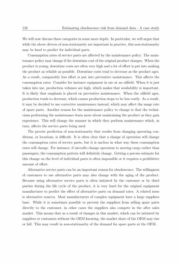
128 Estimating obsolescence risk from demand data - A case study
We will now discuss these categories in some more depth. In particular, we will argue that
while the above drivers of non-stationarity are important in practice, this non-stationarity
may be hard to predict for individual parts.
Consumption rates of service parts are affected by the maintenance policy. The main-
tenance policy may change if the downtime cost of the original product changes. When the
product is young, downtime costs are often very high and a lot of effort is put into making
the product as reliable as possible. Downtime costs tend to decrease as the product ages.
As a result, comparably less effort is put into preventive maintenance. This affects the
consumption rates. Consider for instance equipment in use at an oilfield. When it is just
taken into use, production volumes are high, which makes that availability is important.
It is likely that emphasis is placed on preventive maintenance. When the oilfield ages,
production tends to decrease, which causes production stops to be less costly. As a result,
it may be decided to use corrective maintenance instead, which may affect the usage rate
of spare parts. Another reason for the maintenance policy to change is that the techni-
cians performing the maintenance learn more about maintaining the product as they gain
experience. This will change the manner in which they perform maintenance which, in
turn, affects the service parts being used.
The precise prediction of non-stationarity that results from changing operating con-
ditions, or locations, is difficult. It is often clear that a change of operation will change
the consumption rates of service parts, but it is unclear in what way these consumption
rates will change. For instance, if aircrafts change operation to moving cargo rather than
passengers, the consumption pattern will definitely change. Getting a precise estimate for
this change on the level of individual parts is often impossible or it requires a prohibitive
amount of effort.
Alternative service parts can be an important reason for obsolescence. The willingness
of customers to use alternative parts may also change with the aging of the product.
Because using alternative service parts is often initiated by the customer or by third
parties during the life cycle of the product, it is very hard for the original equipment
manufacturer to predict the effect of alternative parts on demand rates. A related issue
is alternative sources. Most manufacturers of complex equipment have a large suppliers
base. While it is sometimes possible to prevent the suppliers from selling spare parts
directly to the customer, in other cases the suppliers also compete in the after sales
market. This means that as a result of changes in this market, which can be initiated by
suppliers or customers without the OEM knowing, the market share of the OEM may rise
or fall. This may result in non-stationarity of the demand for spare parts at the OEM.
6.3 Analysis of service part demand data 129
Manufacturers strive for standardization across products of the same type for logistical,
as well as a number of other reasons, but customer requirements may cause them to vary
the configuration across products of the same type, which may also influence obsolescence.
For example, when a single customer changes his maintenance policy or the operating
conditions at a customer change, the change in demand for parts that are used across the
entire installed base might not be that large, but the change in demand for parts that
are only used in the products used by that customer will be much larger. The relative
demand non-stationarity caused by the factors we discussed above may thus be amplified
by variations across the installed base.
To summarize this discussion of demand non-stationarity: there are a number of
reasons for spare parts to experience significant demand decreases, as well as increases,
while the product is still in use. It is hard to precisely predict in advance the moment at
which these demand changes occur. However, discussions with the employees of the OEM
revealed that the above reasons for demand non-stationarity do occur at the OEM, even
though it is hard to quantify each of them. They also revealed that the above drivers of
non-stationarity may cause very significant demand decreases, to the extent of rendering
the stocks effectively obsolete.
6.3 Analysis of service part demand data
To get closer to the problem of obsolescence in practice, we will analyze the demand
data and the inventory assortment of spare parts at the company. For the analysis we
use a large data set consisting of the demand for all service parts used in a single type
of product manufactured by the OEM. The product consists of a very large number of
parts that can possibly be replaced (> 30000). Each time a service part is needed, the
date at which the part was needed, together with the part number and the quantity is
registered. To get rid of interchangeability issues the data were preprocessed, treating
different service parts that are interchangeable as a single service part. The parts that
were used for large preventive maintenance (PM) actions, in which a large fraction of
the installed base is enhanced in a short time interval, were filtered out as well. The
usages that were kept correspond mostly to corrective maintenance and condition based
maintenance. We cannot rule out the possibility that some parts used for PM actions
remain, but they are certainly not a large fraction of the usages. Also, parts for which the
moment that they would become obsolete was known in advance were filtered out. Some
parts used in this product type are also used in other product types. We performed some
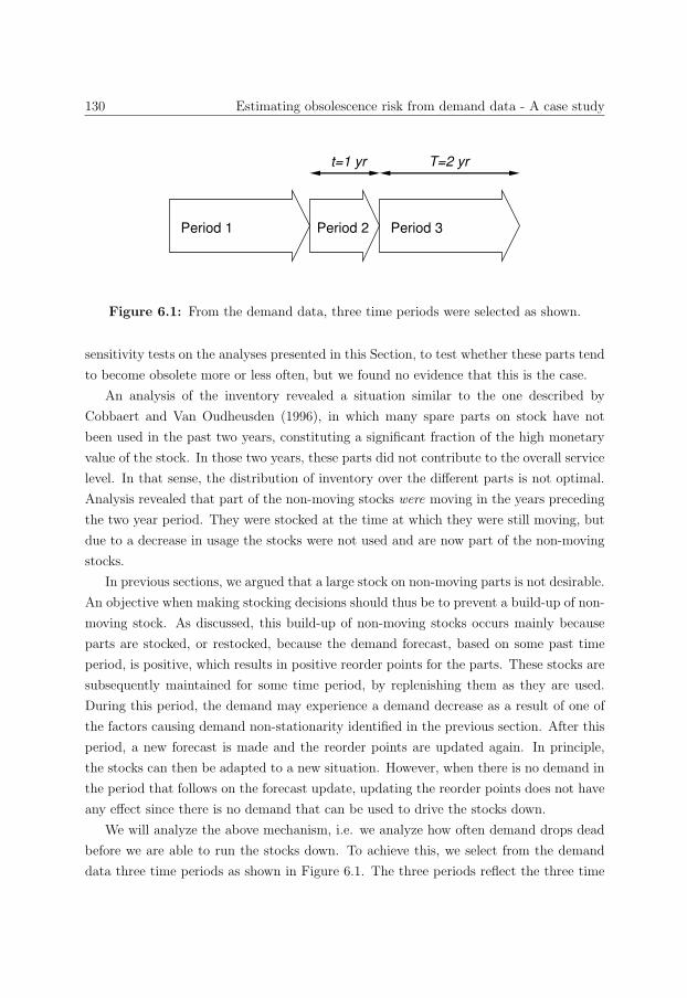
130 Estimating obsolescence risk from demand data - A case study
t=1 yr T=2 yr
Period 1 Period 2 Period 3
Figure 6.1: From the demand data, three time periods were selected as shown.
sensitivity tests on the analyses presented in this Section, to test whether these parts tend
to become obsolete more or less often, but we found no evidence that this is the case.
An analysis of the inventory revealed a situation similar to the one described by
Cobbaert and Van Oudheusden (1996), in which many spare parts on stock have not
been used in the past two years, constituting a significant fraction of the high monetary
value of the stock. In those two years, these parts did not contribute to the overall service
level. In that sense, the distribution of inventory over the different parts is not optimal.
Analysis revealed that part of the non-moving stocks were moving in the years preceding
the two year period. They were stocked at the time at which they were still moving, but
due to a decrease in usage the stocks were not used and are now part of the non-moving
stocks.
In previous sections, we argued that a large stock on non-moving parts is not desirable.
An objective when making stocking decisions should thus be to prevent a build-up of non-
moving stock. As discussed, this build-up of non-moving stocks occurs mainly because
parts are stocked, or restocked, because the demand forecast, based on some past time
period, is positive, which results in positive reorder points for the parts. These stocks are
subsequently maintained for some time period, by replenishing them as they are used.
During this period, the demand may experience a demand decrease as a result of one of
the factors causing demand non-stationarity identified in the previous section. After this
period, a new forecast is made and the reorder points are updated again. In principle,
the stocks can then be adapted to a new situation. However, when there is no demand in
the period that follows on the forecast update, updating the reorder points does not have
any effect since there is no demand that can be used to drive the stocks down.
We will analyze the above mechanism, i.e. we analyze how often demand drops dead
before we are able to run the stocks down. To achieve this, we select from the demand
data three time periods as shown in Figure 6.1. The three periods reflect the three time
6.3 Analysis of service part demand data 131
periods in the mechanism that leads to the build-up of dead stock, as described in the
previous paragraph. Time Period 1 reflects the period on which the forecast is based. At
the beginning of Period 2 the reorder points based on this forecast start to be used. At
the end of Period 2, the reorder points are updated again based on a new forecast. During
Period 3, the stocks can be adapted to the new reorder points. This cannot be achieved
if there is no demand in Period 3, in which case the reorder points that were taken into
use at the beginning of Period 2 may have caused a build-up of dead stock.
To perform the experiment, we need to decide on the length of the time periods. The
length of Period 2 corresponds to the period during which a set of reorder points is in use.
At the company, this period differs depending on the part. For slow moving parts, it is
reasonable to assume that the reorder points are updated each year. We thus choose the
length of Period 2 to be one year. The length of Period 1 is chosen in such a way that
the total usage of the underlying product is the same for Period 1 and Period 3, and it
is only slightly shorter than the length of Period 3 (two years), because the usage of the
underlying product is more or less constant. The total usage of service parts is also equal
over Period 1 and 3. When forecasting the demand for slow moving parts, the company
uses a moving average based on a demand period of around two years. Therefore, setting
the length of Period 1 at around two years is a good choice.
In the experiment, we try to assess the risk of stocking based on a certain number of
orders in a forecast period. The service parts were thus grouped based on the demand in
Period 1, i.e. on the demand in the forecast period. For each of the groups it was assessed
how many parts did not have any demand in Period 3. It is important to note that the
fact that a part does not have any demand in Period 3 does not necessarily mean that the
part is obsolete. We will make a distinction between parts that are obsolete, and parts
that are not obsolete but have zero demand in Period 3 because of statistical variation.
Clearly, the outcomes of the analysis depend on the time intervals for which we do the
analysis. The probability of zero demand in Period 3 might increase or decrease for this
application when the time windows shift, or, said otherwise, as time passes. To assess
this effect, we will do two analyses, which differ because we let the time periods start two
years earlier in the second analysis.
To obtain insight in the distinction between zero demand caused by temporary demand
variations and zero demand because of demand non-stationarity, we will compare the
fraction of parts in a group for which there is zero demand in Period 3 with the fraction
of parts in the group which should have zero demand if demand followed a (compound)
Poisson process in Period 3, with a rate following the forecast based on the number
of orders in Period 1. This latter fraction serves as a benchmark, that determines which
132 Estimating obsolescence risk from demand data - A case study
# of orders # of Actual fraction of parts with Benchmark: Fraction of partsin Period 1 parts no demand in Period 3 with zero demand (Poisson)
1 5630 57.5% (55.4%) e−1 ≈ 36.8%2 2434 35.2% (34.4%) e−2 ≈ 13.5%3 1340 18.2% (20.5%) e−3 ≈ 5.0%4 809 13.1% (14.0%) e−4 ≈ 1.8%5 690 6.8% (7.9%) e−5 ≈ 0.7%6 482 5.0% (5.1%) e−6 ≈ 0.2%7 401 4.0% (3.3%) e−7 ≈ 0.1%8 292 1.4% (3.0%) e−8 ≈ 0.0%9 259 0.8% (1.0%) e−9 ≈ 0.0%≥ 10 1664 0.2% (0.2%) ≤ e−10 ≈ 0.0%
Table 6.1: Outcomes of the analysis of the demand for service parts. The numbers in
parenthesis show the outcome when we let the analysis start two years earlier, shifting all
time periods by two years.
fraction of parts that drop dead is attributable to statistical variation. In the next Section
we will give a motivation for the use of the Poisson process as a benchmark.
The results of the analysis are shown in Table 6.1. This table shows that most parts
are slow moving, in the sense that they were used only a few times in Period 1. This is
typical for service parts in complex products. By looking at the third and fourth column
of Table 6.1 we conclude that demand drops dead more often than would be expected
based on the stationary Poisson assumption, an indication that the probability can not
be entirely explained by temporary demand variations. Furthermore, by comparing the
numbers in the third column with the numbers in parenthesis in that column, we conclude
that the probability of demand dropping dead is quite stable over time.
There are different explanations for a part to have zero demand in Period 3 in Table 6.1.
Since, according to the Poisson distribution, there is a significant probability of zero
demand in Period 3 for some groups, it is plausible that there was a temporary demand
decrease for some parts that did not have any demand in Period 3, causing their demand
to be zero for two years. In light of the discussion on obsolescence in the previous sections,
and in light of the fact that the fraction of parts that had zero demand in each group
exceeds the probability of zero demand according to the Poisson distribution, it is plausible
that some parts that did not have any demand in Period 3 became obsolete.
No data are available at the company which allows for a distinction between these
cases for all parts in Table 6.1. Being obsolete is thus unobservable, or, at least, very hard
to observe with certainty, because doing so requires an in-depth study for each individual
6.3 Analysis of service part demand data 133
part, looking into the different causes of demand non-stationarity that were identified
in the previous section, and checking whether these cases are applicable for the part in
question. We can only observe that the parts are not used anymore. Only future demand
can reveal whether the part remains unused, or whether the part is needed again.
In order to strengthen the case that some of the parts that had zero demand in Period
3 are indeed obsolete, we assess the demand in a fourth period, with a length of four
years, immediately after Period 3. We assess which fraction of the parts in Table 6.1
which had zero demand in Period 3, also have zero demand in Period 4. We found that
this fraction is as high as 50%. As a comparison, we also assess which fraction of the
parts in Table 6.1 which have positive demand in Period 3 have zero demand in Period 4.
We found a fraction equal to 9%.
Thus, a high fraction of the parts that had zero demand in Period 3 turn out to
remain non-moving for another four years. This indicates that the demand rate in Period
2 has indeed changed for some of the parts that had zero demand in Period 3. Indeed, in
light of the discussion in previous sections it is logical to explain a large fraction of parts
that stop moving for six years as being an indication of demand non-stationarity rather
than trying to explain it using a demand model that does not take into account demand
non-stationarity.
The data thus confirms that obsolescence of service parts also occurs while the product
is still in use. This may result in high costs, because any money spent to obtain unused
service parts is lost. These costs are costs in addition to costs of tied up capital and
warehouse costs. An approach sometimes used in industry is therefore to add obsolescence
costs to the holding costs of service parts. This implies an assumption of the same risk of
obsolescence for all parts. Table 6.1 shows that this assumption is not very precise: there
are large differences in the risk of service parts becoming obsolete even for parts used in
the same product type. It seems that slow moving parts become obsolete more often than
fast moving parts. In the remainder of this chapter, we will propose a method to include
this knowledge in an inventory model.
As a final remark, we wish to note that while the groups in Table 6.1 are solely
determined based on the number of orders in Period 1, additional classification can be
achieved by including additional part characteristics in the class definition. By including
characteristics that affect the obsolescence risk in the classification, we could increase
the discriminating power of the method. For the application that we have in mind,
including whether the part is an electronic part or a structural part slightly increases
the discriminating power of the method. However, adding this additional characteristic
decreases the size of the classes, and the added value of adding the characteristic does
134 Estimating obsolescence risk from demand data - A case study
not seem to weigh up against the increased error in the estimates of the obsolescence risk
because of this size decrease.
6.4 The method
In this section, we will describe a method that can be used to determine the risk of
obsolescence from demand data. We start by motivating the use of a particular demand
model, and we give a formal description of the demand model. Subsequently, the method
that can be used to extract the risk of obsolescence for the model is described. The section
is concluded with some remarks on the implementation of the method at the company, and
with an illustration of the advantage of applying the model over applying more traditional
models.
6.4.1 Modeling discussion
In this Section, we will motivate the modeling choices that were made. We will also
consider some alternative modeling possibilities, and explain why they are less suitable
for our purpose.
To use the demand model for inventory control, we will need the demand distribution
during leadtime. We start by arguing that, to model demand in such short time intervals
(most leadtimes are shorter than a few months), it is suitable to use a (compound) Poisson
process. At the end of Section 6.2, we distinguished between temporary demand devia-
tions, and demand non-stationarity. On the short term, it is reasonable to assume that
only temporary demand deviations play a role. When determining how to model short
term demand, we thus only need to consider the variabilities typically associated with
temporary demand variations, as described at the end of Section 6.2. These variabilities
are largely independent between different pieces of equipment. Because there are many
pieces of equipment, it is reasonable to assume that on the short term, the demand has
the memoryless property. Finally, on the short term we don’t expect significant demand
changes, so at this point we restrict ourselves to stationary demand.
It is thus reasonable to model the short term demand as a stationary, memoryless
process. In addition, we would like the demand model to be discrete in nature, reflecting
that the demand for spare parts is discrete as well. The above properties that we would like
the short term demand model to have point us towards the compound Poisson model, since
it has all these properties. In addition, the compound Poisson model has the advantage of
6.4 The method 135
making the resulting inventory problem tractable. It is not surprising that the (compound)
Poisson demand model is the standard demand model for spare parts.
In the previous Section, the (compound) Poisson model was used a benchmark to
test whether the probability of zero demand in Period 3 could be explained by tempo-
rary demand variations. The above also serves as a motivation to use the model as a
benchmark.
Note that the above arguments are not meant to show that the compound Poisson pro-
cess is the only correct model for short term demand, nor to that it is the only benchmark
to test whether the probability of zero demand can be attributed to temporary demand
variations. They merely serve to show that using the compound Poisson process for these
purposes is a reasonable thing to do.
The short term demand can thus be modeled as a compound Poisson process. In
previous sections, we discussed that employees of the company feel that demand for spare
parts is non-stationary. Drivers for demand non-stationarity were identified, and we
have shown that the demand data confirms that the demand is non-stationary. Also, we
identified a mechanism in which non-stationary demand causes a build-up of dead stock.
The costs incurred in this way are not part of most inventory models, as those models
assume that demand is stationary. Since these costs are significant, we wish to include
them into the model. To accomplish this, we will develop a demand model that includes
demand non-stationarity. Moreover, we will develop a method to extract from Table 6.1
the parameters needed to apply this method.
Song and Zipkin (1993) provide a framework which incorporates the possibility of sud-
den changes in demand rate. They let the demand rate in a Poisson demand model depend
on the state of an underlying Markov process, representing the ‘state of the world’. In
light of the discussion in Section 6.2, their model is attractive because state transitions in
their model could correspond to changes in operating conditions, maintenance policy, the
introduction of alternative parts, or changes in the market for spares, while the variabil-
ity in the Poisson process itself can account for the temporary demand variations. The
framework leaves much freedom in determining the precise structure of the underlying
Markov chain. The framework would allow for a part to visit multiple underlying ‘states
of the world’, before ending up to become obsolete.
For models in which multiple states have a positive demand rate, it is not straight-
forward to estimate the parameters. The only method we could think of to estimate
the parameters would be hidden Markov theory (see e.g. Rabiner (1988)). While these
techniques have proven powerful, implementing the hidden Markov algorithms requires a
lot of effort, and a lot of data is needed to obtain reliable estimates for the parameters.
136 Estimating obsolescence risk from demand data - A case study
Even after aggregating demand over different parts, it is doubtful whether we would have
enough demand data for successful estimation of the parameters.
For the purpose of making the model aware of the risk of stocking slow moving parts,
such a model is however not needed. Instead, we propose the use of a simpler, two-state
model, with only one state in which the part is moving. In the other state, demand for
the part has dropped dead. This last state is assumed to be an absorbing state.
The advantages of such a simple Markov model are threefold. First, it is possible to
estimate the parameters for this model in a far simpler manner, and less data suffices
for estimating the parameters. Also, the method has only one additional parameter in
comparison to more standard demand models, and this parameter has a simple, intuitive
interpretation. Finally, when the parameters of the model are known, the optimization
of this model is far simpler.
Using a simpler model also brings disadvantages. While in reality, we also observe
demand increases, and more gradual demand decreases than sudden obsolescence, the
model excludes both of these possibilities. If we use the two-state model to accommodate
for the increased probability of zero demand in Table 6.1, the model will predict an overall
decrease in demand in Period 3 with respect to Period 1. In practice, the demand over all
parts remains about equal in Period 3 with respect to Period 1. More states would allow
us to model the possibility of demand increases, as well as allowing us to keep the total
demand (in the model) over all parts equal while modeling the increased variability in
the demand of individual parts. Models with more states would also allow us to model a
gradual decrease towards obsolescence Song and Zipkin (1993). In summary, the two-state
model should be viewed as an approximation to reality, but clearly a better approximation
that a stationary compound Poisson process, which is the model often used in practice.
Besides multi-state Markov modulated Poisson processes, we wish to consider one ad-
ditional alternative modeling of the demand. It might be possible to explain the increased
probability of zero demand in Period 3 in Table 6.1 by assuming the number of orders is
not Poisson distributed, but has a higher variance to mean ratio. The main disadvantage
of this approach is that it is unclear how we should translate this higher variance to mean
ratio to model the demand distribution over leadtime. Moreover, the memoryless property
of the demand is necessarily lost, which will complicate analysis of the resulting model.
Also, in light of the discussions in earlier sections, it makes sense to let obsolescence be
a part of the model, instead of using an alternative explanation that does not include
obsolescence.
In this contribution, we thus focus on the two-state Markov modulated compound
Poisson model. We believe that, while this model still can be improved to match closer
6.4 The method 137
to reality, it represents a significant step towards application of models including obsoles-
cence. Most importantly, the model improves on the standard compound Poisson model
because of its awareness of the possibility of obsolescence.
The model
We assume that the demand rate depends on the state of a continuous time Markov
process. This Markov process has two states: x0 and x1. In state x1 the demand is
healthy, in state x0 demand has dropped dead. State x0 is an absorbing state. Apart
from the parameters that govern the demand in state x1, the Markov process introduces
one additional parameter that corresponds to the rate at which the system moves from the
first to the second state. This parameter will be denoted by ψ. Furthermore, we assume
that as long as the system is in state x1, demand will follow a (compound) Poisson process
with rate λ and compounding distribution D. We assume P (D > 0) = 1. The state of the
Markov chain at time t will be denoted by X(t) ∈ {x0, x1}. The demand in the interval
(t, t′) will be denoted by C(t, t′).
Estimating the parameters
If we want to apply the model at the mentioned company, we need an estimate for the
parameters λ, D and ψ for each part. In this section, we develop such a method. To
obtain the parameters λ and D we use demand data from a recent period, that serves as
a forecasting period. λ can be estimated by using the number of orders in this period. D
can be fitted by using the mean and the variance of the size of the orders in this period
and by subsequently fitting on these values some distribution that is deemed appropriate.
Now, the parameter ψ, that can be identified with the short term risk of obsolescence,
remains to be determined.
To determine ψ we assume that the short term future behavior of parts with a certain
number of orders in the forecasting period will be similar to the short term future behavior
of parts with the same number of orders in a similar period in the past. The reason for this
assumption is that we have observed that the numbers in the third column of Table 6.1
do not depend to a great degree on the point in time at which we let the first time interval
start.
We will thus use the information we gathered for the different groups in Table 6.1 to
estimate the obsolescence rate ψ. Table 6.1 however does not give an estimate for the
parameter ψ, but an estimate for the probability of zero demand in a certain time interval,
i.e. Period 3 in Figure 6.1. To arrive at the parameter ψ we will calculate the probability
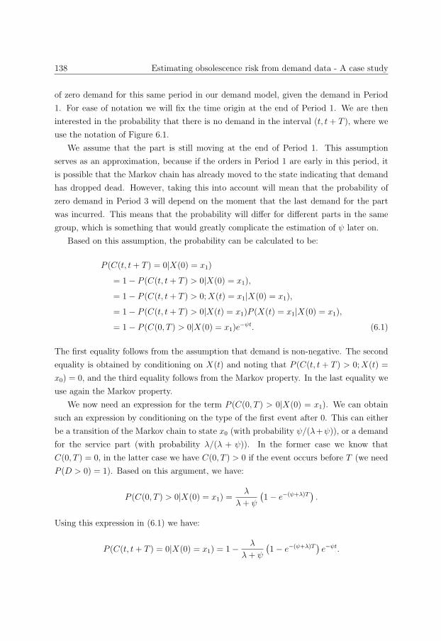
138 Estimating obsolescence risk from demand data - A case study
of zero demand for this same period in our demand model, given the demand in Period
1. For ease of notation we will fix the time origin at the end of Period 1. We are then
interested in the probability that there is no demand in the interval (t, t + T ), where we
use the notation of Figure 6.1.
We assume that the part is still moving at the end of Period 1. This assumption
serves as an approximation, because if the orders in Period 1 are early in this period, it
is possible that the Markov chain has already moved to the state indicating that demand
has dropped dead. However, taking this into account will mean that the probability of
zero demand in Period 3 will depend on the moment that the last demand for the part
was incurred. This means that the probability will differ for different parts in the same
group, which is something that would greatly complicate the estimation of ψ later on.
Based on this assumption, the probability can be calculated to be:
P (C(t, t+ T ) = 0|X(0) = x1)
= 1− P (C(t, t+ T ) > 0|X(0) = x1),
= 1− P (C(t, t+ T ) > 0;X(t) = x1|X(0) = x1),
= 1− P (C(t, t+ T ) > 0|X(t) = x1)P (X(t) = x1|X(0) = x1),
= 1− P (C(0, T ) > 0|X(0) = x1)e−ψt. (6.1)
The first equality follows from the assumption that demand is non-negative. The second
equality is obtained by conditioning on X(t) and noting that P (C(t, t + T ) > 0;X(t) =
x0) = 0, and the third equality follows from the Markov property. In the last equality we
use again the Markov property.
We now need an expression for the term P (C(0, T ) > 0|X(0) = x1). We can obtain
such an expression by conditioning on the type of the first event after 0. This can either
be a transition of the Markov chain to state x0 (with probability ψ/(λ+ψ)), or a demand
for the service part (with probability λ/(λ + ψ)). In the former case we know that
C(0, T ) = 0, in the latter case we have C(0, T ) > 0 if the event occurs before T (we need
P (D > 0) = 1). Based on this argument, we have:
P (C(0, T ) > 0|X(0) = x1) =λ
λ+ ψ
(1− e−(ψ+λ)T
).
Using this expression in (6.1) we have:
P (C(t, t+ T ) = 0|X(0) = x1) = 1− λ
λ+ ψ
(1− e−(ψ+λ)T
)e−ψt.
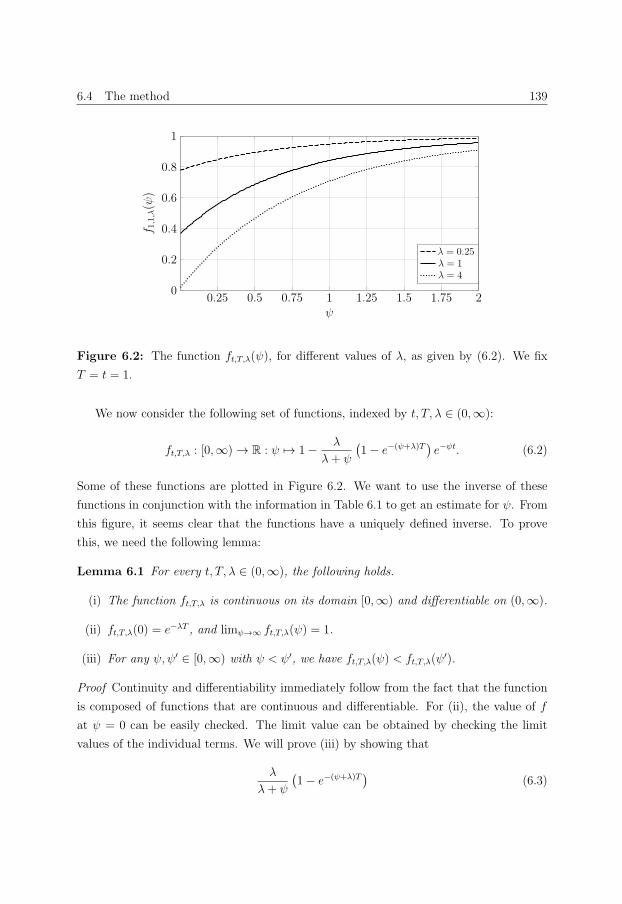
6.4 The method 139
0.25 0.5 0.75 1 1.25 1.5 1.75 20
0.2
0.4
0.6
0.8
1
ψ
f 1,1,λ(ψ
)
λ = 0.25λ = 1λ = 4
Figure 6.2: The function ft,T,λ(ψ), for different values of λ, as given by (6.2). We fix
T = t = 1.
We now consider the following set of functions, indexed by t, T, λ ∈ (0,∞):
ft,T,λ : [0,∞)→ R : ψ �→ 1− λ
λ+ ψ
(1− e−(ψ+λ)T
)e−ψt. (6.2)
Some of these functions are plotted in Figure 6.2. We want to use the inverse of these
functions in conjunction with the information in Table 6.1 to get an estimate for ψ. From
this figure, it seems clear that the functions have a uniquely defined inverse. To prove
this, we need the following lemma:
Lemma 6.1 For every t, T, λ ∈ (0,∞), the following holds.
(i) The function ft,T,λ is continuous on its domain [0,∞) and differentiable on (0,∞).
(ii) ft,T,λ(0) = e−λT , and limψ→∞ ft,T,λ(ψ) = 1.
(iii) For any ψ, ψ′ ∈ [0,∞) with ψ < ψ′, we have ft,T,λ(ψ) < ft,T,λ(ψ′).
Proof Continuity and differentiability immediately follow from the fact that the function
is composed of functions that are continuous and differentiable. For (ii), the value of f
at ψ = 0 can be easily checked. The limit value can be obtained by checking the limit
values of the individual terms. We will prove (iii) by showing that
λ
λ+ ψ
(1− e−(ψ+λ)T
)(6.3)
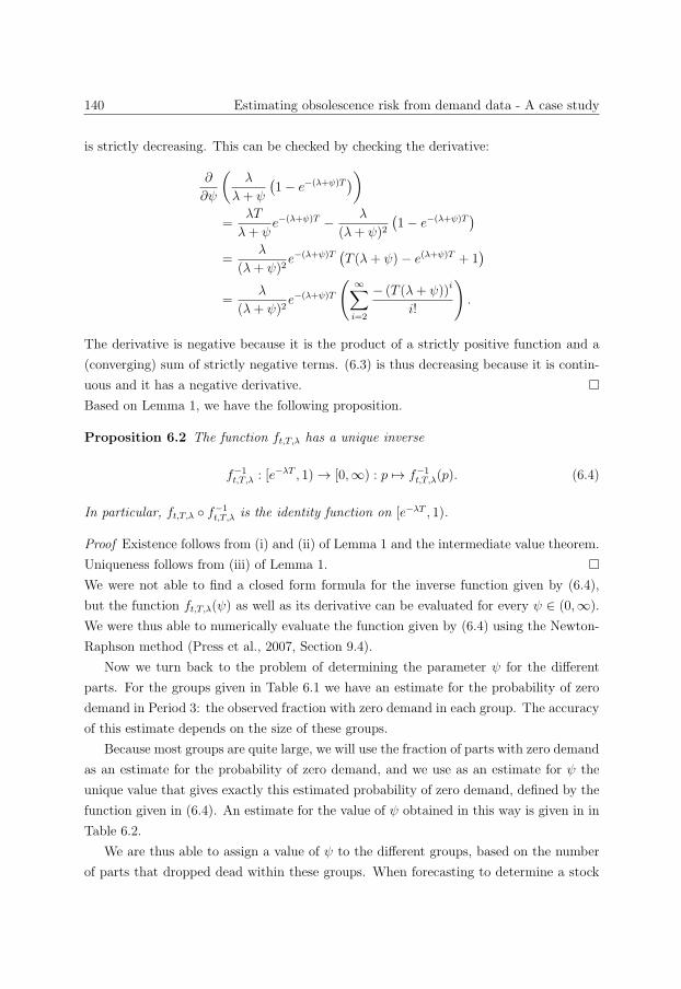
140 Estimating obsolescence risk from demand data - A case study
is strictly decreasing. This can be checked by checking the derivative:
∂
∂ψ
(λ
λ+ ψ
(1− e−(λ+ψ)T
))
=λT
λ+ ψe−(λ+ψ)T − λ
(λ+ ψ)2(1− e−(λ+ψ)T
)=
λ
(λ+ ψ)2e−(λ+ψ)T
(T (λ+ ψ)− e(λ+ψ)T + 1
)
=λ
(λ+ ψ)2e−(λ+ψ)T
( ∞∑i=2
− (T (λ+ ψ))i
i!
).
The derivative is negative because it is the product of a strictly positive function and a
(converging) sum of strictly negative terms. (6.3) is thus decreasing because it is contin-
uous and it has a negative derivative. �Based on Lemma 1, we have the following proposition.
Proposition 6.2 The function ft,T,λ has a unique inverse
f−1t,T,λ : [e−λT , 1)→ [0,∞) : p �→ f−1t,T,λ(p). (6.4)
In particular, ft,T,λ ◦ f−1t,T,λ is the identity function on [e−λT , 1).
Proof Existence follows from (i) and (ii) of Lemma 1 and the intermediate value theorem.
Uniqueness follows from (iii) of Lemma 1. �We were not able to find a closed form formula for the inverse function given by (6.4),
but the function ft,T,λ(ψ) as well as its derivative can be evaluated for every ψ ∈ (0,∞).
We were thus able to numerically evaluate the function given by (6.4) using the Newton-
Raphson method (Press et al., 2007, Section 9.4).
Now we turn back to the problem of determining the parameter ψ for the different
parts. For the groups given in Table 6.1 we have an estimate for the probability of zero
demand in Period 3: the observed fraction with zero demand in each group. The accuracy
of this estimate depends on the size of these groups.
Because most groups are quite large, we will use the fraction of parts with zero demand
as an estimate for the probability of zero demand, and we use as an estimate for ψ the
unique value that gives exactly this estimated probability of zero demand, defined by the
function given in (6.4). An estimate for the value of ψ obtained in this way is given in in
Table 6.2.
We are thus able to assign a value of ψ to the different groups, based on the number
of parts that dropped dead within these groups. When forecasting to determine a stock
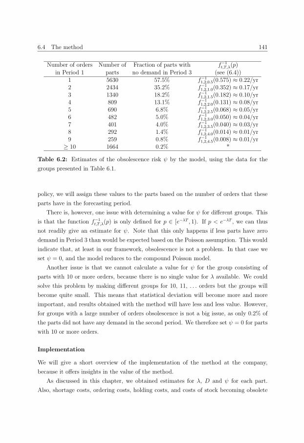
6.4 The method 141
Number of orders Number of Fraction of parts with f−1t,T,λ(p)
in Period 1 parts no demand in Period 3 (see (6.4))1 5630 57.5% f−11,2,0.5(0.575) ≈ 0.22/yr2 2434 35.2% f−11,2,1.0(0.352) ≈ 0.17/yr3 1340 18.2% f−11,2,1.5(0.182) ≈ 0.10/yr4 809 13.1% f−11,2,2.0(0.131) ≈ 0.08/yr5 690 6.8% f−11,2,2.5(0.068) ≈ 0.05/yr6 482 5.0% f−11,2,3.0(0.050) ≈ 0.04/yr7 401 4.0% f−11,2,3.5(0.040) ≈ 0.03/yr8 292 1.4% f−11,2,4.0(0.014) ≈ 0.01/yr9 259 0.8% f−11,2,4.5(0.008) ≈ 0.01/yr≥ 10 1664 0.2% *
Table 6.2: Estimates of the obsolescence risk ψ by the model, using the data for the
groups presented in Table 6.1.
policy, we will assign these values to the parts based on the number of orders that these
parts have in the forecasting period.
There is, however, one issue with determining a value for ψ for different groups. This
is that the function f−1t,T,λ(p) is only defined for p ∈ [e−λT , 1). If p < e−λT , we can thus
not readily give an estimate for ψ. Note that this only happens if less parts have zero
demand in Period 3 than would be expected based on the Poisson assumption. This would
indicate that, at least in our framework, obsolescence is not a problem. In that case we
set ψ = 0, and the model reduces to the compound Poisson model.
Another issue is that we cannot calculate a value for ψ for the group consisting of
parts with 10 or more orders, because there is no single value for λ available. We could
solve this problem by making different groups for 10, 11, . . . orders but the groups will
become quite small. This means that statistical deviation will become more and more
important, and results obtained with the method will have less and less value. However,
for groups with a large number of orders obsolescence is not a big issue, as only 0.2% of
the parts did not have any demand in the second period. We therefore set ψ = 0 for parts
with 10 or more orders.
Implementation
We will give a short overview of the implementation of the method at the company,
because it offers insights in the value of the method.
As discussed in this chapter, we obtained estimates for λ, D and ψ for each part.
Also, shortage costs, ordering costs, holding costs, and costs of stock becoming obsolete
142 Estimating obsolescence risk from demand data - A case study
were defined in consultation with the management. The former three costs are relatively
standard, the latter costs consist of all costs incurred by the company when stock becomes
obsolete. Subsequently, recommendations for the reorder point and the order-up-to point
were given by minimizing the total expected costs. This resulted in reorder points and
order up to points that could be imported in the erp system. These recommendations
are generally followed by the inventory controllers.
In comparison to the approach where the obsolescence costs are spread evenly over
all parts by including them as a constant factor in the holding cost, the model has a
clear advantage. This advantage lies in the fact that the model knows that stocking slow
moving parts is more costly than stocking faster moving parts, because of the higher risk
of obsolescence. In comparison to the simpler approach, the model will thus stock more
faster moving parts, and less slower moving parts. This improvement was also recognized
by the inventory controllers, who in general follow the recommendations coming from the
new system. Simulation results using real demand data on which we will not report in
detail also indicate that including the risk on obsolescence improves the recommendations.
Illustration of the advantage of the method
In order to illustrate the manner in which the knowledge of obsolescence risk can improve
the recommendations given by the model, we will give some results on two hypothetical,
but realistic parts S and F. Both parts have a price of 4000. When the part becomes
obsolete, it cannot be used anymore. To determine the costs we should associate with
this, we should remember that the fact that the part is obsolete is often not observable.
It is therefore likely that the part will be stocked for some time even after it has become
obsolete, which results in stocking costs. When it becomes clear that the part is obsolete,
we have to handle it, for instance by scrapping it. The total costs of this may exceed
the procurement price of the part. We assume the costs for a part becoming obsolete are
5000.
Both parts have a leadtime of one year. Both parts are demanded only in quantity 1,
so we assume pure Poisson demand for both. We assume full back-ordering, and a back
order cost of 365× 200 per part per year. For simplicity, we assume a base stock policy.
Now, part S is a slow mover, as it has had two orders in the last two years, while part F
has had 14 orders in the last two years.
We proceed to find cost estimates for different base stock levels according to two
different models. The naive model is a model in which holding costs of 25% are taken
into account for both parts, in which 5% obsolescence cost is naively included. This gives
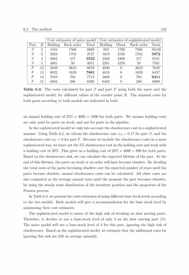
6.4 The method 143
Cost estimates of naive model Cost estimates of sophisticated modelPart R Holding Back order Total Holding Obsol. Back order TotalS 2 1104 7566 8669 883 1700 7566 10149S 3 2023 1704 3727 1619 2550 1704 5872S 4 3004 317 3322 2403 3400 317 6121S 5 4001 50 4051 3201 4250 50 7501F 12 5049 3610 8659 4040 0 3610 7649F 13 6022 1639 7661 4818 0 1639 6457F 14 7010 704 7713 5608 0 704 6311F 15 8004 286 8290 6403 0 286 6689
Table 6.3: The costs calculated for part S and part F using both the naive and the
sophisticated model, for different values of the reorder point R. The minimal costs for
both parts according to both models are indicated in bold.
an annual holding cost of 25% × 4000 = 1000 for both parts. We assume holding costs
are only paid for parts on stock, and not for parts in the pipeline.
In the sophisticated model we take into account the obsolescence cost in a sophisticated
manner. Using Table 6.2, we obtain the obsolescence rate ψS = 0.17 for part S, and the
obsolescence rate ψF = 0 for part F . Because we include the obsolescence costs in a more
sophisticated way, we leave out the 5% obsolescence cost in the holding cost and work with
a holding cost of 20%. This gives us a holding cost of 20% × 4000 = 800 for both parts.
Based on the obsolescence risk, we can calculate the expected lifetime of the part. At the
end of this lifetime, the parts on stock or on order will have become obsolete. By dividing
the total costs of the parts becoming obsolete over the expected number of years until the
parts become obsolete, annual obsolescence costs can be calculated. All other costs are
also computed as the average annual costs until the moment the part becomes obsolete,
by using the steady state distribution of the inventory position and the properties of the
Poisson process.
In Table 6.3, we present the costs estimates of using different base stock levels according
to the two models. Both models will give a recommendation for the base stock level by
minimizing their cost estimates.
The sophisticated model is aware of the high risk of stocking on slow moving parts.
Therefore, it decides to use a base-stock level of only 3 on the slow moving part (S).
The naive model will use a base-stock level of 4 for this part, ignoring the high risk of
obsolescence. Based on the sophisticated model, we estimate that the additional costs for
ignoring this risk are 249 on average annually.
144 Estimating obsolescence risk from demand data - A case study
Something similar happens with the faster moving part (F). The sophisticated model
knows there is no significant risk of this item becoming obsolete, and therefore stocking
on the part is relatively cheap. It will therefore use a base-stock level of 14 for this part.
The naive model uses a higher obsolete cost for this part, not knowing that this part will
probably not become obsolete. Therefore, it stocks too conservatively, which will cost an
additional 146 annually based on the estimate by the sophisticated model.
6.5 Conclusions and extensions
We have presented a method that can be used to estimate the risk of obsolescence using
demand data. The method is based upon observations in the demand data of service parts
that are used in products with a long life cycle. In principle, the method can be applied
by any company with sufficient data for a sufficient number of parts, and products with
long life cycles. However, more research is needed to find out if other companies have
similar demand patterns for service parts. In particular, it would be interesting to find
out whether a similar analysis as the one used in Section 6.3 gives similar results at other
companies, in the sense that the number of parts in each group that have zero demand
in the second period exceed the number of parts that should have zero demand according
to the Poisson model. The method was implemented at the company, and the resulting
order suggestions were in general followed by the inventory controllers.
It would be interesting to extend the method to Markov models with more than 2
states, examples of which are considered by Song and Zipkin (1996b). While this allows
us to model demand increases as well as decreases, multiple states will greatly complicate
the estimation of the model parameters from the demand data. The theory of hidden
Markov models (see, e.g. Rabiner (1988)) might prove useful in this respect.
Chapter 7
Finding optimal policies in (S − 1, S)
lost sales inventory models with
multiple demand classes
This chapter examines the algorithms proposed by Kranenburg and Van Houtum (2007a)
for finding good critical level policies in the (S − 1, S) lost sales inventory model with
multiple demand classes. Our main result is that we establish guaranteed optimality for
two of these algorithms. This result is extended to different resupply assumptions, such
as a single server queue. As a corollary, we provide an alternative proof of the optimality
of critical level policies among the class of all policies.
7.1 Introduction
In many inventory systems, customers belong to different classes, for instance differing in
their willingness to pay for fast delivery of their orders. In order to increase their profits,
some companies provide different customer classes with different levels of service. This
can be achieved by using inventory rationing, a concept in which inventory is withheld
from less demanding, lower profit customer classes to preserve it for future, more critical
demands. A related concept is a critical level policy, in which each customer class is
assigned a critical level. When stock is below the critical level assigned to a particular
customer class, the stock is withheld from that customer class and preserved for more
important customer classes.
The problem of multiple demand classes was first described by Veinott (1965), who
also introduced critical level policies. Topkis (1968) shows optimality of critical level
146 Optimizing (S − 1, S) inventory models with multiple demand classes
policies for a system with generally distributed demand, periodic review and zero leadtime,
in which case the critical levels depend on the time until the next review. Ha (1997)
considers critical level policies in a make-to-stock system with lost demand, under a
Poisson demand assumption. The production decision is an integral part of the model. He
established optimality of critical levels and shows that demands of the highest criticality
should always be satisfied. Furthermore, he shows that a base stock policy is optimal for
managing production. This work was extended to the back-ordering case by De Vericourt
et al. (2002).
Dekker et al. (2002) consider the optimization of the critical levels and the base stock
level for a problem with independent leadtimes. They derive expressions for the costs of a
given critical level base stock policy. Subsequently, they derive bounds for the base stock
level S on the basis of which the optimal critical level policy can be found, by solving the
optimization problem for each possible S by explicit enumeration. Explicit enumeration is
prohibitively slow for problems with many demand classes and large S. Therefore, Dekker
et al. (2002) propose a fast approach to find good critical levels for which optimality is
not guaranteed. For the case of two demand classes, Melchiors et al. (2000) extend this
work to fixed quantity ordering. Deshpande et al. (2003) consider a similar model, but
with back-ordering of unsatisfied demand. The order in which back-ordered demands are
satisfied leads to additional complications.
Continuing along the lines of Dekker et al. (2002), Kranenburg and Van Houtum
(2007a) consider optimization of the critical levels and the base-stock level. Similarly to
Dekker et al. (2002), the problem is split up into a number of sub-problems for fixed S.
Kranenburg and Van Houtum propose three algorithms for solving these sub-problems.
In an extensive numerical experiment, they find that these algorithms are much faster
(in the order of 200-1000 times as fast for problems with 2 to 5 demand classes) than
complete enumeration. Moreover, the algorithms appear to find optimal solutions. Based
on this, they conjecture without proof that the algorithms are optimal for all possible
instances.
This chapter examines the algorithms proposed by Kranenburg and Van Houtum
(2007a) for finding good critical level policies in the (S − 1, S) lost sales inventory model
with multiple demand classes. These algorithms resemble local search algorithms; for a
precise description we refer to Section 7.4, or to the mentioned article. A question arising
from their contribution is whether these algorithms can get stuck in a local optimum.
We will answer this question negatively; we prove that the algorithms result in optimal
solutions. This is a surprising result, because non-randomized local searches are known
to get stuck in local optima in many other problems. We extend this result to a make-
7.2 The model 147
to-stock queue in which a base-stock level is fixed and we search for the optimal critical
levels. As a corollary we establish the optimality of critical level policies, recovering and
strengthening a result that was essentially derived by Miller (1969). To obtain the results,
we rely on theory on undiscounted Markov decision problems to derive results regarding
the structure of the bias of “locally optimal” critical level policies. Ultimately, we show
that the bias of such policies solve the optimality equations.
Kranenburg and Van Houtum argue that there is a need for fast and accurate algo-
rithms, and they show that their algorithms are fast. Our main contribution is that these
algorithms can now be used in certainty that optimal solutions will be obtained. Fur-
thermore, we show that the same general theory used for establishing structural results
in many inventory models can also be used to devise fast special purpose algorithms for
finding the optimal policy in inventory models. Lastly, we show that critical levels are
optimal among the class of all policies for the model we consider.
The remainder of this chapter is organized as follows. The model is formulated as a
Markov decision process in Section 7.2. We then restate some general results from Markov
decision theory in Section 7.3. The optimality of the algorithms is proved in Section 7.4.
Some extensions are discussed in Section 7.5. Section 7.6 concludes.
7.2 The model
We consider the model studied earlier by Dekker et al. (2002) and Kranenburg and Van
Houtum (2007a). They use minimization of the long term average cost as optimality
criterion. To comply with the convention used in Puterman (1994), we will interpret
the costs as negative rewards and use maximization of the long term average reward as
optimality criterion. Clearly, these two formulations are equivalent.
Demands for a part are classified according to criticality. Let J be the set of demand
classes (|J | ≥ 1). For each class j ∈ J , demands occur according to a Poisson process
with rate mj > 0. If an item is not delivered to class j upon request, the demand is lost
and a penalty cost pj > 0 is to be paid, which will be interpreted as a negative reward.
Classes are numbered 1, 2, . . . , |J | such that p1 ≥ p2 ≥ . . . ≥ p|J |. The item is stored in a
single stock location, and stock for the item is controlled by an order-up-to-S policy. We
denote the state of the system by k ∈ {0, . . . , S}, where k denotes the number of items
on order. The heuristics of which we will prove optimality find critical levels for fixed S.
We also assume fixed S, but for optimization purposes S can be enumerated in a separate
loop using the bounds derived by Dekker et al. (2002).
148 Optimizing (S − 1, S) inventory models with multiple demand classes
Kranenburg and Van Houtum (2007a, Remark 1) make the important observation that
under linear holding costs in the amount of stock on hand, we can assume without loss
of generality that holding costs are also charged for items in replenishment. Under this
assumption, the holding costs do not depend on the control of the system for fixed S, and
can be omitted when considering optimization of the critical levels.
We assume i.i.d. exponential leadtimes. In Section 7.5 we show how to extend this
assumption to the assumption of i.i.d. general leadtimes, as long as the control of the
system is restricted to be of a certain type. We denote the rate by which new parts arrive
in state k by νk = kL−1, where L is the expected leadtime. For convenience of notation,
we include ν0 = 0 in this definition.
In order to model the problem as a Markov decision problem, we consider more general
policies than the critical level policies to which Kranenburg and Van Houtum (2007a)
restrict their attention. We let Ak be the set of Markovian deterministic decision rules in
state k. Each decision rule a ∈ Ak prescribes which demand classes to accept and which
to reject in state k. For k < S, each a ∈ Ak is denoted as a subset of the set of demand
classes J . E.g. if a = {1, 3, 4} is selected as the decision rule in state k, then this denotes
that under rule a demand classes 1, 3 and 4 are accepted and other demand classes are
rejected in state k. Thus, Ak is isomorphic with the powerset P(J) of J . In state S all
demands are necessarily rejected. AS thus consists only of the empty set. A Markovian
deterministic stationary policy consists of a decision rule a ∈ Ak for each state k. A policy
will be denoted by d = (d(0), . . . , d(S)) ∈ A0 × . . . × AS = DMD. We will consider only
stationary policies, a restriction that we will motivate in the following.
Because the time intervals between successive events are exponential, the problem
can be modeled as a continuous time Markov decision process. Under the assumption
that the control is only changed when transitions occur (a weak condition that can still
be weakened), uniformization can be applied and the model can be transformed into a
discrete-time Markov decision process which is equivalent in terms of long term average
reward (see e.g. Puterman (1994, Section 11.5.3)). We will apply this transformation, and
work with the transformed model. Under conditions valid for this discrete time model,
Puterman (1994, Theorem 8.4.5) shows that there exists a stationary deterministic average
optimal policy, which motivates our restriction to policies of this type.
The states of the transformed model are the same as the states of the original model.
For a complete description of the discrete time model we further need the rewards and
transition probabilities in state k under decision a ∈ Ak. After transforming the model,
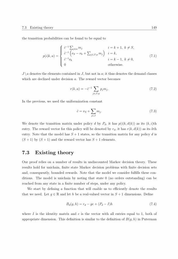
7.3 Existing theory 149
the transition probabilities can be found to be equal to
p(i|k, a) =
⎧⎪⎪⎪⎪⎨⎪⎪⎪⎪⎩
c−1∑
j∈a mj i = k + 1, k = S,
c−1(νS − νk +
∑j∈J\a mj
)i = k,
c−1νk i = k − 1, k = 0,
0 otherwise.
(7.1)
J \a denotes the elements contained in J , but not in a; it thus denotes the demand classes
which are declined under decision a. The reward vector becomes
r(k, a) = −c−1∑j∈J\a
pjmj. (7.2)
In the previous, we used the uniformization constant
c = νS +∑j∈J
mj. (7.3)
We denote the transition matrix under policy d by Pd, it has p(i|k, d(k)) as its (k, i)th
entry. The reward vector for this policy will be denoted by rd, it has r(k, d(k)) as its kth
entry. Note that the model has S + 1 states, so the transition matrix for any policy d is
(S + 1) by (S + 1) and the reward vector has S + 1 elements.
7.3 Existing theory
Our proof relies on a number of results in undiscounted Markov decision theory. These
results hold for unichain, finite state Markov decision problems with finite decision sets
and, consequently, bounded rewards. Note that the model we consider fulfills these con-
ditions. The model is unichain by noting that state 0 (no orders outstanding) can be
reached from any state in a finite number of steps, under any policy.
We start by defining a function that will enable us to efficiently denote the results
that we need. Let g ∈ R and let h be a real-valued vector in S + 1 dimensions. Define
Bd(g, h) = rd − ge+ (Pd − I)h (7.4)
where I is the identity matrix and e is the vector with all entries equal to 1, both of
appropriate dimension. This definition is similar to the definition of B(g, h) in Puterman
150 Optimizing (S − 1, S) inventory models with multiple demand classes
(1994, Equation 8.4.3), except that it does not include the maximum over all decisions
d ∈ D and therefore it depends on d.
When a policy d ∈ DMD is fixed, the model reduces to a Markov reward process. For
the model under consideration, this Markov reward process induces a unique long term
average reward gd and a bias vector hd. These quantities satisfy a relation that will be
exposed in the following lemma.
Lemma 7.1 For a given policy d ∈ DMD, the Markov decision problem reduces to a
Markov reward process with transition matrix Pd and reward vector rd. The average
expected reward gd and bias {hd}Sk=0 of this unichain Markov reward process satisfy
Bd(gd, hd) = 0. (7.5)
Furthermore, this equation determines gd uniquely, and hd up to an overall constant.
Proof The result is a slight reformulation of Corollary 8.2.7 of Puterman (1994) and the
remarks following it. �Now, we will establish a link between the reward of two policies. To this end, we will
need the limiting matrix which we will discuss here first. The results we state here can be
found in Puterman (1994, Appendix A.4). Let P ∗d denote the limiting matrix associated
with Pd
P ∗d = limN→∞
1
N
N∑t=1
P t−1d .
Denote the (k, i)th element of this matrix by p∗d(i|k). For unichain Markov reward pro-
cesses, this matrix has equal rows, and its elements are given by p∗d(i|k) = p∗d(i), where
p∗d(i) is the long term fraction of time that the system is in state i under policy d. For
recurrent states under policy d, p∗d(i) > 0. Because p∗d(i|k) does not depend on the initial
state k, the long term average expected reward does not depend on the initial state either.
This is reflected by the fact that the average expected reward vector has equal elements.
It is given by gde = P ∗d rd. P ∗d satisfies P ∗dPd = P ∗d . Note also that in a finite state space
P ∗d is a stochastic matrix: P ∗d e = e. These two equations can be used to find the steady
state probabilities. The relation gde = P ∗d rd can subsequently be used to find the long
term average reward associated with policy d.
The following result uses the limiting matrix to establish a link between the average
reward of two policies. It will be pivotal in proving a key property of the bias of the
policies found by the algorithms of which we will prove the optimality.
7.4 Optimality of the algorithms 151
Lemma 7.2 Let d ∈ DMD and let gd and hd be the gain and bias associated with d. Let
d′ denote another policy (∈ DMD) with associated average expected reward gd′. Let P ∗d′denote the limiting matrix associated with Pd′. Then we have
gd′e = gde+ P ∗d′Bd′(gd, hd).
Proof We adapt the proof of Proposition 8.6.1 of Puterman (1994). We know that gd′e =
P ∗d′rd′ . We add and subtract gde at the right hand side of this equation. Now, we note
that P ∗d′(Pd′ − I) = 0 and P ∗d′e = e, and obtain
gd′e = gde+ P ∗d′ (rd′ − gde+ (Pd′ − I)hd) .
The result can be easily recognized using (7.4). �The next lemma gives conditions under which a policy is optimal.
Lemma 7.3 Let d ∈ DMD and let gd and hd be the gain and bias associated with d. If
maxd′∈DMD
Bd′(gd, hd) = 0 (7.6)
then gd is the optimal average expected reward, and d is an optimal policy attaining this
reward.
Proof gd is the optimal reward by Puterman (1994, Theorem 8.4.1 c). Now, note that
Bd(gd, hd) = 0 by Lemma 7.1, which means that d attains the maximum in (7.6). We now
apply Puterman’s (1994) Theorem 8.4.4 to conclude optimality of d. �
7.4 Optimality of the algorithms
Because Algorithm 1 and 2 proposed in Section 5 of Kranenburg and Van Houtum (2007a)
only terminate when they find a local optimum, the policies they find have a number of
properties, which we formalize in the following definition. (The algorithms themselves are
listed before Theorem 7.7.)
Definition 7.1 A policy d will be said to belong to the locally optimal critical level policies
DL if it has the following two properties
1. d is of critical level type, viz, for each demand class j ∈ J there exists a critical
level cj ∈ {0, . . . , S}, such that demands of class j are accepted when k < S − cj,
and declined when k ≥ S − cj. So j ∈ d(k) if and only if k < S − cj. Furthermore,
152 Optimizing (S − 1, S) inventory models with multiple demand classes
the critical levels are monotone in demand criticality, i.e. i > j ⇒ ci ≥ cj. Note
that these critical levels fully determine a policy, but that not every policy can be
described by a set of critical levels.
2. d is locally optimal, in the sense that a unit increase or decrease of any single
critical level such that monotonicity is not violated does not result in an increase of
the average expected reward.
In the following, we will use the lemmas from the previous section to establish the opti-
mality of policies d ∈ DL. First, we need to obtain a form for Bd(g, h) specific for our
model. It is straightforward, but it requires some precision and tenacity, to use (7.1),
(7.2) and (7.3) to find the following expression for the kth element of Bd(g, h) as defined
in (7.4):
(Bd(g, h))(k) =− g + c−1(−νk [h(k)− h(k − 1)]
−∑
j∈J\d(k)pjmj +
∑j∈d(k)
mj [h(k + 1)− h(k)]
). (7.7)
We have introduced the variables h(−1) = 0 and h(S+1) = 0 for convenience of notation,
which necessarily have a pre-factor 0 since d(S) = ∅ and ν0 = 0. In the following lemma,
we show that the Markov reward process induced by a locally optimal critical level policy
has a bias with a certain structure.
Lemma 7.4 Suppose d ∈ DL. Let gd and hd be the gain and bias associated with d. Let
j ∈ J with associated critical level cj be given.
1. Suppose cj = S. Then hd(S − cj)− hd(S − cj − 1) ≥ −pj.
2. Suppose cj = 0. Then hd(S − cj + 1)− hd(S − cj) ≤ −pj.Proof For i), suppose first that d can be modified by increasing cj by 1 without violating
monotonicity. Call this modified policy d′. It differs from d only by a unit increase of cj.
d′ thus only differs from d because it rejects demands of class j in state S− cj − 1 instead
of accepting them, viz,
(d′(0), . . . , d′(S − cj − 1), . . . , d′(S)) = (d(0), . . . , d(S − cj − 1) \ {j}, . . . , d(S)).
Using this observation, we can use (7.7) to show that
Bd′(g, h) = Bd(g, h)− eS−cj−1c−1mj(h(S − cj)− h(S − cj − 1) + pj) (7.8)
7.4 Optimality of the algorithms 153
where eS−cj−1 is the vector with 1 as its (S− cj−1)th entry, and zero for all other entries.
Now, we apply Lemma 7.2, and in the second equality we use (7.8) and Lemma 7.1.
gd′e = gde+ P ∗d′Bd′(gd, hd)
= gde− P ∗d′(eS−cj−1c−1mj(hd(S − cj)− hd(S − cj − 1) + pj)).
Referring to the discussion regarding the limiting matrix P ∗d in Section 7.3 we conclude
that
gd′e =(gd − p∗d′(S − cj − 1)c−1mj(hd(S − cj)− hd(S − cj − 1) + pj)
)e. (7.9)
p∗d′(S−cj−1) denotes the long term average fraction of time spent in state S−cj−1. It is
strictly positive because demands for class j are accepted in class 0 trough S−cj−2 underpolicy d′, from which we infer that S − cj − 1 is recurrent. mj > 0 by assumption. Since
d′ differs from d only in the unit decrease of a single critical level, we have gd − gd′ ≥ 0
by d ∈ DL. From (7.9), h(S− cj)− h(S− cj − 1)+ pj must be non-negative as well, from
which the result immediately follows.
Now suppose that increasing cj violates monotonicity. Then, let j′ be the demand class
with the least penalty cost, for which cj′ = cj. It is easy to verify from the definitions
that the critical level cj′ can be increased without violating monotonicity. Now, apply the
argument above for j′. We find that
h(S − cj′)− h(S − cj′ − 1) + pj′ ≥ 0
which directly implies the result since pj′ ≤ pj and cj′ = cj by hypothesis.
The proof of ii) is similar. Suppose d′ can be constructed from d by a unit decrease
of cj without violating monotonicity. Then d′ differs from d because it accepts demands
for class j in state S − cj instead of declining them. Thus
Bd′(g, h) = Bd(g, h) + eS−cj c−1mj(h(S − cj + 1)− h(S − cj) + pj).
Similarly as before
gd′e = gde+ p∗d′(S − cj)c−1mj(h(S − cj + 1)− h(S − cj) + pj)e
from which the result follows readily. Suppose now that cj cannot be decreased without
violating monotonicity. Then, let j′ be the demand class with the highest penalty cost, for
154 Optimizing (S − 1, S) inventory models with multiple demand classes
which cj′ = cj. c′j can be increased without violating monotonicity, and we can proceed
as before to conclude that the result continues to hold. �Lemma 7.4 can be intuitively understood by using the interpretation of hd(k)− hd(k− 1)
as the comparative advantage of being in state k instead of being in state k − 1 under
policy d.
In the following lemma, we prove that the bias of the Markov reward process induced
by a locally optimal policy is concave and strictly decreasing in the number of outstanding
orders.
Lemma 7.5 Suppose d ∈ DL. Let gd and hd be the gain and bias associated with d. Then
1. For k ∈ {0, . . . , S − 1}
hd(k + 1)− hd(k) < 0
2. For k ∈ {1, . . . , S − 1}
hd(k + 1)− hd(k) ≤ hd(k)− hd(k − 1)
Proof We start by proving 1 for k = 0. From the definition of the critical levels we must
either have a critical level cj for which S− cj = 0, or all demands are accepted in state 0.
In the first case, we apply ii) of Lemma 7.4 to conclude that hd(1)− hd(0) ≤ −pj < 0. In
the latter case we note first that gd and hd solve (7.5) by Lemma 7.1, which implies that
0 = (Bd(gd, hd))(0).
By using (7.7) and by noting that d(0) = J for the case under consideration this implies
that
0 = c−1∑j∈J
mj (hd(1)− hd(0))− gd.
It is easy to see that under any policy there must be at least one recurrent state in which
demands are declined. Therefore, gd is strictly negative. Furthermore, c > 0, |J | ≥ 1 and
mj > 0. The result follows.
We now prove 2 for k = 1 (suppose S > 0). From the definition of the critical levels
we either have a critical level cj for which S − cj = 1, or all demand classes accepted
7.4 Optimality of the algorithms 155
in state 0 are also accepted in state 1 and vice versa. The result immediately follows by
combining i) and ii) of Lemma 7.4 in the former case. In the latter case we use again
that gd and hd solve (7.5), from which it follows that
0 = (Bd(gd, hd))(1)− (Bd(gd, hd))(0).
since both terms on the right hand side are zero. Using d(1) = d(0) for the case we are
considering and (7.7) we find that this implies that
c−1∑j∈d(0)
mj (hd(2)− 2hd(1) + hd(0)) = c−1ν1 (hd(1)− hd(0)) .
The right hand side is strictly negative by i) for k = 0. Clearly, d(0) = ∅ contradicts
negativity of the right hand side. We conclude that d(0) = ∅, and the result follows.
We now proceed by induction. Note that 1 for k follows from 2 for k and 1 for k − 1.
To complete our inductive argument, it thus suffices to show that 2 for k ∈ {1, . . . , S− 1}follows from 1 and 2 for k − 1.
Again, we either have a critical level cj for which S− cj = k, or the demands accepted
in state k are also accepted in state k − 1 and vice versa. In the former case, the result
follows immediately by combining i) and ii) of Lemma 7.4, so we do not need the induction
hypothesis in this case. In the latter case, we have d(k) = d(k − 1). Again
0 =(Bd(gd, hd))(k)− (Bd(gd, hd))(k − 1)
which holds by Lemma 7.1, implies for k ∈ {1, . . . , S − 1} that∑j∈d(k)
mj [hd(k + 1)− 2hd(k) + hd(k − 1)]
= νk [hd(k)− hd(k − 1)]− νk−1 [hd(k − 1)− hd(k − 2)] . (7.10)
The right hand side of this equation can be shown to be equal to
νk−1 [hd(k)− 2hd(k − 1) + hd(k − 2)] + (νk − νk−1) [hd(k)− hd(k − 1)]
The first term is not positive by the induction hypothesis ii) for k−1, and the second term
is strictly negative by induction hypothesis i) for k−1 and by νk−νk−1 > 0. So, d(k) = ∅leads to a contradiction, and we conclude that d(k) = ∅ and hd(k+1)−2hd(k)+hd(k−1) ≤0. By induction, the result follows. �
156 Optimizing (S − 1, S) inventory models with multiple demand classes
In the following lemma, we use the results derived in the previous two lemmas to show that
a policy d that is of locally optimal critical level type satisfies the optimality equations.
Therefore, it is also globally optimal.
Lemma 7.6 Let d ∈ DL. Then d is an optimal policy, and the average expected reward
associated with d is the optimal reward.
Proof Let gd and hd denote the average expected reward and bias of the Markov reward
process induced by d. The hypotheses of Lemmas 7.4 and 7.5 are satisfied for hd. To
show that the hypothesis of Lemma 7.3 is satisfied we need to show that
maxd′∈DMD
Bd′(gd, hd)
equals the 0-vector. Since gd and hd satisfy (7.5) by Lemma 7.1, it is equivalent to show
that for each k ∈ {0, . . . , S} the following expression
maxd′∈DMD
(Bd′(gd, hd))(k)− (Bd(gd, hd))(k) (7.11)
equals 0. For k = S, this holds trivially since AS only consists of one element (∅), reflectingthat all demands are necessarily lost in state S. Now consider the case k < S. Using
(7.7) and remembering that DMD is the Cartesian product of the decision sets Ak for the
different states, it is straightforward to show that (7.11) is equivalent to
maxd′(k)∈Ak
⎛⎝ ∑
j∈d′(k)∩(J\d(k))mj [h(k + 1)− h(k) + pj]
−∑
j∈(J\d′(k))∩d(k)mj [h(k + 1)− h(k) + pj]
⎞⎠ . (7.12)
where equal terms were cancelled. Note that d′(k)∩ (J \ d(k)) denotes the demands that
are accepted under d′ but declined under d in state k.
Take now an arbitrary demand class j ∈ J \ d(k) that is declined under d in state k.
We will show that h(k + 1) − h(k) + pj is non-positive. d is of critical level type, so by
definition 7.1 there exists a critical level cj for demand class j. Since j is declined under
d in state k, it is a matter of checking this definition to establish that the critical level cj
for j satisfies S − cj ≤ k. Note that this implies that S − cj ≤ S − 1. We thus can apply
7.4 Optimality of the algorithms 157
ii) of Lemma 7.4 to conclude that
hd(S − cj + 1)− hd(S − cj) ≤ −pj.
By applying ii) of Lemma 7.5 repeatedly and by using that S − cj ≤ k we conclude that
hd(k + 1)− h(k) ≤ hd(S − cj + 1)− hd(S − cj).
Combining the above equations yields the result. The first term in (7.12) is thus non-
positive.
Take now an arbitrary demand j ∈ d(k). It can be shown in a very similar manner
as above that h(k + 1) − h(k) + pj is nonnegative. cj now satisfies S − cj > k, implying
S − cj > 0. We then apply i) of Lemma 7.4, and continue as before.
When including the minus sign, the second term in (7.12) is thus non-positive as well.
Therefore, the maximum is bounded from above by 0. Now, note that d′(k) = d(k) attains
the bound, from which we conclude that the maximum equals 0. We conclude that the
hypothesis of Lemma 7.3 is satisfied. The result now immediately follows. �We are now ready to prove the optimality of the algorithms proposed by Kranenburg
and Van Houtum (2007a). Kranenburg and Van Houtum show that it is never optimal
to decline the most critical demand classes, which will be denoted by {1, . . . , jc} where
jc = max{j ∈ J |p1 = pj}. We now summarize the algorithms proposed in Kranenburg
and Van Houtum (2007a), adapted where needed to our notation and the fact that we
have used a reward model
Algorithm 1. Keep cj, j ∈ J , j ≤ jc always fixed at 0. Start with an arbitrary
choice for cj, j ∈ J , j > jc, that satisfies monotonicity. Define the neighborhood as
all policies that still satisfy the monotonicity constraint and that have critical levels
that differ at most one from the corresponding critical levels in the original policy. If
the reward of the cheapest neighbor is strictly larger than the reward of the current
solution, then select this neighbor and set this policy as the current solution, and
repeat the process of evaluating all neighbors for this new policy. Otherwise, stop
and take the current solution as the solution found by the algorithm.
Algorithm 2. Keep cj, j ∈ J , j ≤ jc always fixed at 0. Start with an arbi-
trary choice for cj, j ∈ J , j > jc, that satisfies monotonicity. For j = |J |, findcj ∈ {cj−1, . . . , cj+1} with the highest reward, at fixed values of the other critical
levels, and change ci accordingly (define c|J |+1 = S). When the reward for the cur-
rent solution ties with the best alternative, keep the current solution. Repeat this
158 Optimizing (S − 1, S) inventory models with multiple demand classes
optimization for one critical level at a time for j = |J | − 1 down to jc + 1. After
that, optimize again for j = |J |. Continue this iterative process until for none of
the j-values (> jc) a strict improvement is found. This is the solution found by the
algorithm.
The following theorem establishes the optimality of Algorithms 1 and 2.
Theorem 7.7 Algorithms 1 and 2 converge in a finite number of steps. When they
terminate, the final solution is optimal among the class of Markovian deterministic policies
in general, and in particular among the class of critical level policies.
Proof We show that the policy found upon termination of the above algorithms belongs
to DL. Then Lemma 7.6 guarantees optimality of this policy. A policy dt found upon
termination of either of these algorithms is clearly of critical level type. Also, for both
algorithms, decreasing or increasing a single critical level for a demand class j > jc does
not increase the average expected reward because this would contradict the termination
of the algorithm.
In order for dt to belong to DL, it remains to check that a unit increase in the critical
level cjc associated with jc decreases the expected reward. This is precisely what is shown
for any policy in Kranenburg and Van Houtum (2007a, Lemma 2) in order to establish
that the optimal critical levels for demand classes j ≤ jc are 0, which motivated them to
keep these critical levels fixed at 0 in the first place. We conclude that dt ∈ DL. The final
solution is thus optimal. To conclude that the algorithms converge in a finite number of
steps, note that a solution that was visited cannot be visited again because that would
contradict that the rewards are strictly increasing. Because there are only a finite number
of critical level combinations, the algorithms must converge in a finite number of steps.
�Note that Lemma 7.6 can serve as the basis to define other local search based algorithms
which are guaranteed to be optimal. We could for instance adapt Algorithm 2 by decreas-
ing the neighborhood to unit increases or decreases in the critical levels.
The following corollary is interesting in our opinion because of the manner in which
it is proven.
Corollary 7.8 A monotone critical level policy is optimal for the problem we consider.
For the most critical demand classes j ≤ jc the optimal critical level is equal to 0.
Proof The result follows immediately from Theorem 7.7, and the fact that Markovian
deterministic policies dominate in the model. �
7.5 Extensions 159
By Kranenburg’s (2007) observation with respect to the holding cost, early work by
Miller (1969) becomes applicable for this model. Miller considers a queueing system with
n servers with equal, exponential service rate and controlled admissions. The reward
incurred differs across different customers, which arrive following a Poisson process. His
objective is to maximize the long term average reward. Depending on the number of
servers that are occupied, the gatekeeper may decide to reject customers to save capacity
for more critical customers. Because Kranenburg and Van Houtum show the holding
costs can be assumed to be fixed for fixed S, it is not hard to see that Miller’s model is
equivalent to the model considered here.
In terms of the model considered here, Miller shows that critical levels are optimal
(even though he does not use the concept of critical level policies), and that demands of
the highest criticality are always accepted. This result differs from the result derived by
Ha (1997), e.g. because Ha’s model assumes a make-to-stock environment, more general
holding costs and it includes discounted models.
7.5 Extensions
General leadtimes
Our model assumes i.i.d. exponential leadtimes. Most results obtained in this chapter can
be extended to the case of generally distributed i.i.d. leadtimes considered by Kranenburg
and Van Houtum (2007a), as long as we restrict the decision to accept or reject demands
to depend only upon the criticality of the demand and the number of parts on stock
(Note that Kranenburg and Van Houtum (2007a) assume that the control of the system
is of critical level type, which imposes an even stronger restriction). The steady state
distribution of outstanding orders and consequently the long term expected reward of
such a policy do not depend upon the distribution of the leadtime. This can for instance
be shown by a queueing theory argument of the type that is employed in Kranenburg and
Van Houtum (2007a), or by the arguments employed in Dekker et al. (2002). Therefore,
a policy that is optimal in the exponential case is also optimal for the general leadtime
case, but only within this restricted class of policies. Therefore, the algorithms continue
to find the optimal critical level policy among the class of critical level policies.
Note that imposing the control to depend only upon the number of outstanding or-
ders is a true restriction for general leadtimes, as information about outstanding orders
may improve the quality of stock control. Ha (2000) delves deeper into this question
by considering the optimal control for Erlang distributed production times in a make-to-
160 Optimizing (S − 1, S) inventory models with multiple demand classes
stock environment. Because of the special properties of this distribution, the size of the
state spaces remains manageable. Teunter and Klein Haneveld (2008) consider general
leadtimes in an (s,Q) system. The complexity of the analysis is kept within bounds by
using the approximative assumption that only the costs up until the arrival of the next
replenishment order are relevant.
Dependent leadtimes
Before, we have assumed i.i.d. exponentially distributed leadtimes. This is equivalent
to stating that the orders are served in a queue with S identical servers with rate L−1.
The problem of inventory rationing however also arises in other settings. Make-to-stock,
equivalent with a single server queue, is assessed by Ha (1997). Other examples include
queues with a number of servers larger than 1, but smaller than S.
Before, we had νk = L−1k. We now assume general νk > 0, but such that νk+1 ≥νk. This includes the examples mentioned above. The reader can verify that the only
properties of νk that were used up to and including Lemma 7.6 were the properties νk > 0
(for instance, to establish that the model is unichain), and νk+1 > νk (in the inductive
argument in the proof of Lemma 7.5). It requires only minor modification of the proof of
Lemma 7.5 to allow for νk+1 = νk.
Lemma 7.9 The results stated in Lemma 7.5 remain valid for general νk, as long as
νk+1 ≥ νk and νk > 0.
Proof All results, except the last inductive argument, remain valid without modification.
In the last inductive argument, a possible issue occurs when νk = νk−1; we can no longer
conclude strict positivity of the right hand side of (7.10), only non-negativity remains.
Note that this still suffices to establish the required result in case d(k) = ∅. However,
d(k) = ∅ no longer leads to contradiction.
Therefore, we consider the case d(k) = ∅ separately. Note that this implies that
d(k + 1) = ∅ as well. From Lemma 7.1 we have
0 =(Bd(gd, hd))(k + 1)− (Bd(gd, hd))(k)
from which it follows that
0 = νk+1 (hd(k + 1)− hd(k))− νk (hd(k)− hd(k − 1)) .
The result immediately follows since νk+1 ≥ νk and hd(k) − hd(k − 1) is negative by the
induction hypothesis. �
7.6 Conclusions 161
Thus, under the assumptions in this section, Lemmas 7.4, 7.5, 7.6 remain valid. Theorem
7.7 and its corollary remain valid, except that Kranenburg and Van Houtum’s Lemma 2
no longer holds. We thus need to consider changing the critical levels for the most critical
demand classes in the search algorithms, and we can no longer keep them fixed at 0.
Note furthermore, that we implicitly assume that the holding cost does not depend on
the rationing decision for fixed S. For the original model, Kranenburg and Van Houtum’s
observation ensures that this assumption can be made without severe restrictions. Their
observation is however not valid for the extended model, and assuming fixed holding costs
for fixed S is more restrictive in those cases. It is valid in practical situations in case the
holding costs are also incurred for parts that are in on order, for instance for repairable
components and other closed loop supply chains.
7.6 Conclusions
We established optimality of 2 of the 3 algorithms proposed by Kranenburg and Van Hou-
tum (2007a). We strengthened this result to include resupply conditions other than the
one considered by Kranenburg and Van Houtum. In the process, we recovered the result
by Miller (1969), strengthening it by allowing for more general resupply assumptions.

Chapter 8
Summary and Conclusions
In this thesis, we studied inventory control of service parts for high-tech capital goods, such
as aircraft, trains, (equipment in) refineries, baggage handling systems, dredging equip-
ment and photolithography systems. Capital goods represent significant investments, and
the operators of the goods rely on their availability while planning their operations. Peri-
ods during which the capital good is not available for production (downtime) are therefore
very undesirable, especially if they occur unplanned. To prevent downtime, maintenance
is carried out on the capital goods. Service parts are used during maintenance to replace
parts of the capital good that are malfunctioning, or that might start malfunctioning
soon. Availability of service parts is thus essential to complete the maintenance in a
timely fashion. However, keeping service parts is very costly, because thousands of differ-
ent service parts are typically needed to support a capital good, and each service part by
itself may already represent a significant investment. Therefore, it is important to keep
enough parts of each type on inventory to ensure against costly downtimes, but not too
many to avoid unnecessary costs. Service parts inventory control is therefore an impor-
tant topic of research for SLF-research and ProSeLo, a Dinalog project in which a number
companies work together with three universities to improve their service logistics. The
research reported in this thesis was partly conducted within these projects.
In the thesis, we develop several analytic models and solution methods to gain insights
in service parts inventory control, and to aid companies in making the right decisions.
We now summarize the main findings of the different chapters of the thesis.
Chapters 2, 3 and 4 all investigate aspects of inventory control when maintenance
activities require multiple different service parts to complete. Chapter 2 analyzes an
industrial problem encountered at a repair shop that maintains aircraft components. Each
repair requires multiple different spare parts to complete. The key performance target for
such repair shops is the timely completion of the component repairs of the different types.
164 Summary and Conclusions
This reveals that a proper inventory model for such a repair shop should focus directly
on this target, instead of focusing on the availability of the service parts, as is customary
in state-of-the-art models. In addition, we argue that ordering multiple parts at once
should be modeled as well, because many parts replaced during component maintenance
are relatively inexpensive. We develop a new MIP formulation of the problem based on
these requirements, which uses indicator variables to linearize the formulation. To handle
the large number of decision variables in this formulation, we propose branch and price
algorithms to solve it. The efficiency of these algorithms is driven by a novel idea to
efficiently solve the pricing problem, based on a proposition that states that there exists a
dominance relation between different policy parameters. Our numerical experiments show
that the algorithms solve problems consisting of thousands of parts and components in
practical time-scales, with optimality gaps that are smaller than 1%. In a computational
study using company data, we find that spare parts based approaches cannot attain
business targets on the level of the component repairs, while the proposed approach does
attain these targets.
The optimization model developed in Chapter 2 is based on two key modeling assump-
tions: Ignoring the possibility of Simultaneous Stock-outs (ISS), and first-come first-serve
(FCFS) allocation of spare parts to component repairs. In Chapter 3, we examine the
effect of ISS and FCFS on the quality of the resulting inventory and allocation poli-
cies. These investigations have other repercussions apart from assessing the quality of the
model developed in Chapter 2. In particular, ISS is commonly used in the analysis and
optimization of assemble-to-order (ATO) systems, and FCFS allocation is often applied
in repair shops and in ATO systems because it is easy to implement and fair. Like the
repair shop inventory problem, performance in ATO systems depends on the simultaneous
availability of multiple stock keeping units of different types.
To assess the quality of the ISS policies we need to benchmark their costs with the costs
of (close-to-)optimal policies. Finding close-to-optimal policies is not trivial, however, be-
cause the expected number of back-orders is a non-separable function of the different
base-stock levels, and because exhaustive search is prohibitively slow for the repair shop
inventory problems and realistically sized ATO systems on which we focus. Therefore, we
develop a novel, exact, stochastic programming (SP) formulation of the inventory opti-
mization problem under FCFS allocation. We propose an algorithm to solve the sample
approximation of this SP, giving us lower and upper bounds on its optimal objective func-
tion. Our experiments show that this approach finds solutions that are close-to-optimal,
even for large systems. Using the algorithm to provide lower bounds, we then assess the
ISS performance for a repair shop case and several ATO cases. We find two problem
165
characteristics governing the performance of ISS: the news-vendor (NV) fractiles of each
demand type (component repair), and the correlation between lead-time demand of dif-
ferent stock keeping units (spare parts). The NV fractile of a demand type is defined
as b/(b + h), where b is the back-order costs associated with the demand type, and h
is the total holding costs of all stock keeping units that are by expectation needed to
satisfy a demand of that type. We find that the performance of the ISS solution for the
service parts inventory case is excellent. For example, loss of optimality is 1 − 2% for
news-vendor fractiles between 0.8 and 0.9, and 0 − 0.5% for news-vendor fractiles above
0.9. These results are explained by the relatively low correlations of lead-time demand of
service parts. In contrast, the ISS solution may be non optimal by as much as 33% for
ATO system cases with a higher leadtime demand correlation.
To investigate the impact of FCFS allocation, we develop a lower bound on the optimal
base-stock policy under optimal allocation, and compare it with our close-to-optimal
policies under FCFS. For the repair shop case, we find that the loss of optimality due
to FCFS is less than 12% when NV fractiles exceed 0.97. Unfortunately, we find that
the lower bound under optimal allocation weakens quickly for lower NV fractiles for the
repair shop case. However, the approach results in much more conclusive insights for
the ATO systems. Our experiments for those systems showed that the loss of optimality
varied between 4 and 18% for average NV fractiles of about 0.8, and between 2 and 12%
as the average NV fractiles increase towards 0.95. Besides average NV fractiles, we find
that the assymmetry of the NV fractiles between similar demand types governs FCFS
performance.
The problem studied in Chapter 2 motivates us to study the average number of spare
parts used to maintain a single component of a given type. In Chapter 4, we develop a
method capable of forecasting this information. The method uses exponential smoothing
to forecast the spare parts needed for maintaining a single type of component, and to
forecast the number of components to be maintained of each type. Combining these two
forecasts gives the number of spare parts needed. We benchmark the forecast accuracy
of this “two-step method” against state-of-the-art methods for spare parts forecasting,
using real demand data from Fokker Services. We find that the two-step method is the
joint winner of the benchmark. Its performance is virtually indistinguishable from the
performance of the method with the best performance. Besides being among the best in
terms of forecast accuracy, the two-step method has a number of distinct advantages over
other state-of-the-art methods, due to its ability to forecast the link between maintenance
activities and spare parts usage. First, this link allows practitioners to ensure that spare
parts inventory control is in line with business objectives on the level of maintenance
166 Summary and Conclusions
tasks, as discussed in Chapter 2. Second, this link allows practitioners to incorporate
prior knowledge into the forecast, concerning the number of maintenance tasks that they
plan to execute. We find that incorporating perfect prior knowledge of this kind decreases
forecast errors by 20% for the Fokker Services data. While perfect prior knowledge is
perhaps optimistic, these results show the potential for improving spare parts forecasts
using information on future planned maintenance tasks.
In Chapter 5 we argue that data from reliability centered maintenance studies is a
very suitable source to estimate downtime costs for spare parts inventory models. How-
ever, attempting to use this data gives rise to complications, because spare parts may
be used in multiple different pieces of equipment, each having different downtime costs.
Also, multiple pieces of equipment may perform the same function together involving
redundancy. We develop a model of the inventory system that can cope with these situ-
ations. We propose two approximations of the amount of downtime in this model. In an
extensive numerical study, we find that these approximations have excellent performance.
We benchmark the performance of the resulting policies with the policies obtained using
simple methods that might be used in practice if the redundancy information is not avail-
able, and find that using the detailed redundancy information can significantly improve
the stocking decision.
In Chapter 6, we investigate how to incorporate the risk of obsolescence into stocking
decisions in practice. We analyze spare parts demand data in order to investigate the
issue, and find evidence for the occurrence of obsolescence, and evidence that slow moving
items have a higher probability to become obsolete. We formulate a simple demand model
based on a two-stage Markov model, in which the second state represents that the part
is obsolete. The risk of obsolescence for a part now corresponds to the rate at which the
Markov Chain moves from the first to the second state. We propose a method to quantify
this risk of obsolescence for a part, based on the behavior of groups of similar parts in the
past. We discuss how to incorporate the risk of obsolescence into the inventory decisions,
and illustrate the value of this approach with an example.
In Chapter 7 we investigate two algorithms proposed by Kranenburg and Van Houtum
(2007a) to find good rationing levels in an (S−1, S) inventory model with multiple demand
classes. In particular, we give a mathematical proof of Kranenburg and Van Houtum’s
conjecture that these algorithms always find the optimal rationing levels. We extend these
results towards different resupply models.
We conclude this chapter with a brief review of the direct practical impact of the
research carried out in this thesis. The model and algorithm described in Chapter 2 were
developed in close collaboration with a repair shop owned by Fokker Services. Initial
167
modeling decisions were based on interviews and in-depth discussions with employees of
the company, and the model was revised and enhanced several times after testing it at
the company. The author has implemented the resulting model in a decision support
tool, which is currently used on a daily basis by the repair shop. Section 2.6 of this thesis
reveals that this tool has a significant positive impact on the ability of the company to cost
efficiently attain business targets with respect to repair turnaround times. Discussions at
a repair shop owned by NedTrain have revealed that implementing the approach at other
repair shops is likely to give similar benefits (Aerts, 2012).
The research in Chapters 3 and 4 answers a number of practical questions concerning
the decision support tool described in Chapter 2. The research in Chapter 3 provides
evidence that the ISS modeling assumption used in the tool has only limited impact on
the quality of the resulting recommendations. In Chapter 4, we find evidence that the
forecast method that is used to apply the tool has similar performance as state-of-the-
art forecast methods, motivating its use in practice. We also investigate the practice of
the company to incorporate information regarding future component maintenance into
the forecast, and find that it can significantly improve forecast accuracy. We therefore
recommend the company to continue and if possible expand this practice.
The model and approximative method described in Chapter 5 have been developed
during a collaboration with a large petrochemical company. The research resulted in an
enhanced stocking rule for the company. The method has also led to a better understand-
ing of the role of spare parts inventories for redundant systems at the company (cf. Van
Jaarsveld and Dekker, 2009) . The research in Chapter 6 was initiated to investigate the
suspicions of employees at an OEM of long life-cycle products that slow moving items have
a larger risk of become obsolete. We find evidence that confirms this theory. The method
we developed to quantify this risk has been implemented by the author in a decision
support system for the OEM, which is currently being used to support decision makers
at the OEM. Table 6.3 illustrates how inventory decisions are enhanced by incorporating
the risk of obsolescence in this manner.

References
AberdeenGroup. The service parts management solution selection report. Aberdeen-
Group, Boston, 2005.
G. Aerts. Personal communication, 2012. (Mr. Aerts is assistent head of support at
NedTrain componentenbeheer).
N. Agrawal and M. A. Cohen. Optimal material control in an assembly system with
component commonality. Naval Research Logistics, 48:409–429, 2001.
Y. Akcay and S. H. Xu. Joint inventory replenishment and component allocation opti-
mization in an assemble-to-order system. Management Science, 50:99–116, 2004.
Y. Akcay and S. H. Xu. personal communication, 2012.
Aviation Week. 10-year global MRO forecast. Aviation week: Overhaul & Maintenance,
17(4):28–31, 2011.
S. Axsater. Inventory Control. Springer, 2nd edition, 2006.
F. Baskett, K. Chandy, R. Muntz, and F. Palacios. Open, closed, and mixed networks of
queues with different classes of customers. Journal of the Association for Computing
Machinery, 22:248–260, 1975.
S. Benjaafar and M. ElHafsi. Production and inventory control of a single product
assemble-to-order system with multiple customer classes. Management Science, 52:
1896–1912, 2006.
F. Bernstein, G. DeCroix, and Y. Wang. The impact of demand aggregation through
delayed component allocation in an assemble-to-order system. Management Science,
57:1154–1171, 2011.
J. R. Birge and F. Louveaux. Introduction to stochastic programming. Springer-Verlag,
New York, 1997.
170 References
C. Boone, C. Graighead, and J. Hanna. Critical challenges of inventory management in
service parts supply: a Delphi study. Operations Management Research, 1:31–39, 2008.
J. Boylan and A. Syntetos. Spare parts management: a review of forecasting research and
extensions. IMA Journal of Management Mathematics, 21:227–237, 2010.
G. W. Brown, J. Y. Lu, and R. J. Wolfson. Dynamic modelling of inventories subject to
obsolescence. Management Science, 11:51–63, 1964.
M. Cantoni, M. Marseguerra, and E. Zio. Genetic algorithms and monte carlo simulation
for optimal plant design. Reliability Engineering & System Safety, 68:29–38, 2000. ISSN
0951-8320.
K. D. Cattani and G. C. Souza. Good buy? delaying end-of-life purchases. European
Journal of Operations Research, 146:216–228, 2003.
S. R. Chakravarthy and A. Gomez-Corral. The influence of delivery times on repairable
k-out-of-N systems with spares. Applied Mathematical Modelling, 33:2368–2387, 2009.
F. Y. Chen and Y. Feng. Optimization and optimality of (s,S) stochastic inventory
systems with non-quasiconvex costs. Probability in the Engineering and Informational
Sciences, 20:287–306, 2006.
F. Cheng, M. Ettl, G. Lin, and D. D. Yao. Inventory-service optimization in configure-
to-order systems. Manufacturing & Service Operations Management, 4:114–132, 2002.
K. L. Cheung and W. Hausman. Multiple failures in a multi-item spare inventory model.
IIE Transactions, 27:171–180, 1995.
K. Cobbaert and D. van Oudheusden. Inventory models for fast moving items subject
to “sudden death” obsolescence. International Journal of Production Economics, 44:
239–248, 1996.
J. Croston. Forecasting and stock control for intermittent demands. Operational Research
Quarterly, 23:289–303, 1972.
S. Dayanik, J.-S. Song, and S. H. Xu. The effectiveness of several performance bounds
for capacitated production, partial-order-service, assemble-to-order systems. Manufac-
turing & Service Operations Management, 5:230–251, 2003.
References 171
T. de Kok. Evaluation and optimization of strongly ideal assemble-to-order systems. In
J. G. Shanthikumar, D. D. Yao, and W. H. M. Zijm, editors, Stochastic Modeling and
Optimization of Manufacturing Systems and Supply Chains, chapter 9, pages 203–242.
Kluwer Acadamic Publishers Group, 2003.
K. S. de Smidt-Destombes, M. C. van der Heijden, and A. van Harten. On the availability
of a k-out-of-N system given limited spares and repair capacity under a condition based
maintenance strategy. Reliability Engineering & System Safety, 83:287–300, 2004.
K. S. de Smidt-Destombes, M. C. van der Heijden, and A. van Harten. On the interaction
between maintenance, spare part inventories and repair capacity for a k-out-of-N system
with wear-out. European Journal of Operational Research, 174:182–200, 2006.
K. S. de Smidt-Destombes, M. C. van der Heijden, and A. van Harten. Availability of
k-out-of-N systems under block replacement sharing limited spares and repair capacity.
International Journal of Production Economics, 107:404–421, 2007.
K. S. de Smidt-Destombes, M. C. van der Heijden, and A. van Harten. Joint optimisa-
tion of spare part inventory, maintenance frequency and repair capacity for k-out-of-N
systems. International Journal of Production Economics, 118:260–268, 2009.
F. de Vericourt, F. Karaesmen, and Y. Dallery. Optimal stock allocation for a capacitated
supply system. Management Science, 48:1486–1501, 2002.
R. Dekker and R. Plasmeijer. On the use of equipment criticality in maintenance op-
timization and spare parts inventory control. In C. Guedes Soares, editor, Advances
in Safety & Reliability, volume 3, pages 1709–1718. ESRA, Pergamon press, Oxford,
England, 1997.
R. Dekker, R. Hill, M. Kleijn, and R. Teunter. On the (S − 1, S) lost sales inventory
model with priority demand classes. Naval Research Logistics, 49:593–610, 2002.
Deloitte (Koudal, P.). The service revolution in global manufacturing industries. Deloitte
Research, 2006.
V. Deshpande, M. Cohen, and K. Donohue. A threshold inventory rationing policy for
service-differentiated demand classes. Management Science, 49:683–703, 2003.
M. Dogru, M. Reiman, and Q. Wang. A stochastic programming based inventory policy
for assemble-to-order systems with application to the w model. Operations Research,
58:849–864, 2010.
172 References
A. Eaves and B. Kingman. Forecasting for the ordering and stock-holding of spare parts.
Journal of the Operational Research Society, 55:431–437, 2004.
A. Efron. Bootstrap methods: another look at the jackknife. Annals of Statistics, 7:1–26,
1979.
M. ElHafsi, H. Camus, and E. Craye. Optimal control of a nested-multiple-product
assemble-to-order system. International Journal of Production Research, 46:5367–5392,
2008.
M. Finkelstein. On systems with shared resources and optimal switching strategies. Re-
liability Engineering & System Safety, 94:1358–1362, 2009.
Y. Gerchak and M. Henig. An inventory model with component commonality. Operations
Research Letters, 5:157–160, 1986.
A. Ghobbar and C. Friend. Evaluation of forecasting methods for intermittent parts de-
mand in the field of aviation: A predictive model. Computers and Operations Research,
30:2097–2114, 2003.
P. Glasserman and Y. Wang. Leadtime-inventory trade-offs in assemble-to-order systems.
Operations Research, 46:858–871, 1998.
V. J. Guide and R. Srivastava. Repairable inventory theory: models and applications.
European Journal of Operational Research, 102:1–20, 1997.
R. Gullu and M. Koksalan. A model for performance evaluation and stock optimization
in a kit management problem. International Journal of Production Economics, 2012.
doi: http://dx.doi.org/10.1016/j.ijpe.2012.01.028.
A. Y. Ha. Inventory rationing in a make-to-stock production system with several demand
classes and lost sales. Management Science, 43:1093–1103, 1997.
A. Y. Ha. Stock rationing in an M/Ek/1 make-to-stock queue. Management Science, 46:
77–87, 2000.
W. H. Hausman, H. L. Lee, and A. X. Zhang. Joint demand fulfillment probability in a
multi-item inventory system with independent order-up-to policies. European Journal
of Operational Research, 109:646–659, 1998.
References 173
R. M. Hill, M. Omar, and D. K. Smith. Stock replenishment policies for a stochastic
exponentially-declining demand process. European Journal of Operational Research,
116:374–388, 1999.
K. Hoen, R. Gullu, G. van Houtum, and I. Vliegen. A simple and accurate approximation
for the order fill rates in lost-sales assemble-to-order systems. International Journal of
Production Economics, 133:95–104, 2011.
K. Huang and T. de Kok. Cost minimization in a periodic review assemble-to-order
system. Working paper, 2011.
M. Jalil, R. Zuidwijk, M. Fleischmann, and J. van Nunen. Spare parts logistics and
installed base information. Journal of the Operational Research Society, 62:442–457,
2011.
J. B. Jasper. Quick response solutions, fedex critical inventory logistics revitalized. Fedex
white paper, FedEx, 2006.
P. Kampstra. Email communication, 2012. (Mr. Kampstra is senior modality performance
manager at the service parts supply chain of Philips Healthcare).
R. Kapuscinski, R. Q. Zhang, P. Carbonneau, R. Moore, and B. Reeves. Inventory
decisions in Dells supply chain. Interfaces, 34:191–205, 2004.
W. Kennedy, J. Wayne Patterson, and L. Fredendall. An overview of recent literature on
spare parts inventories. International Journal of Production Economics, 76:201–215,
2002.
R. M. Knotts. Fault diagnosis from a business perspective. Civil Aircraft Maintenance
and Support, 5:335–347, 1999.
A. Kranenburg and G. van Houtum. Cost optimization in the (S−1, S) lost sales inventorymodel with multiple demand classes. Operations Research Letters, 35:493–502, 2007a.
A. Kranenburg and G. van Houtum. Effect of commonality on spare parts provisioning
costs for capital goods. International Journal of Production Economics, 108:221–227,
2007b.
A. A. Kranenburg and G. van Houtum. Service differentiation in spare parts inventory
management. Journal of the Operations Research Society, 59:946–955, 2008.
174 References
A. A. Kranenburg and G. van Houtum. A new partial pooling structure for spare parts
networks. European Journal of Operational Research, 199:908–921, 2009.
W. Kuo and R. Wan. Recent advances in optimal reliability allocation. IEEE Transactions
on Systems, Man, and Cybernetics, 37:143–156, 2007.
S. Li and Z. Li. Spare parts allocation by improved genetic algorithm and monte carlo
simulation. International Journal of Systems Science, 1:1–10, 2010.
J. D. C. Little. A proof for the queuing formula: L = λW . Operations Research, 9:
383–387, 1961.
L. Lu, J.-S. Song, and H. Zhang. Optimal and asymptotically optimal policies for an
assemble-to-order n-system. Working paper, 2012.
Y. Lu and J.-S. Song. Order-based cost optimization in assemble-to-order systems. Op-
erations Research, 53:151–169, 2005.
Y. Lu, J.-S. Song, and D. D. Yao. Order fill rate, leadtime variability, and advance demand
information in an assemble-to-order system. Operations Research, 51:292–308, 2003.
Y. Lu, J.-S. Song, and D. D. Yao. Backorder minimization in multiproduct assemble-to-
order systems. IIE Transactions, 37:763–774, 2005.
Y. Lu, J.-S. Song, and Y. Zhao. No-holdback allocation rules for continuous-time assemble-
to-order systems. Operations Research, 58:691–705, 2010.
W.-K. Mak, D. P. Morton, and R. K. Wood. Monte carlo bounding techniques for deter-
mining solution quality in stochastic programs. Operations Research Letters, 24:47–56,
1999.
M. Marseguerra, E. Zio, and L. Podofillini. Multiobjective spare part allocation by means
of genetic algorithms and monte carlo simulation. Reliability Engineering & System
Safety, 87:325–335, 2005. ISSN 0951-8320.
P. Melchiors, R. Dekker, and M. J. Kleijn. Inventory rationing in an (s,Q) inventory
model with lost sales and two demand classes. Journal of the Operational Research
Society, 51:111–122, 2000.
B. Miller. A queueing reward system with several customer classes. Management Science,
16:234–245, 1969.
References 175
J. R. Moore. Forecasting and scheduling for past-model replacement parts. Management
Science, 18:B200–B213, 1971.
J. Moubray. Reliability-centered Maintenance. Butterworth Heinemann, Oxford, 1991.
J. A. Muckstadt. A model for a multi-item, multi-echelon, multi-indenture inventory
system. Management Science, 20:472–481, 1973.
E. Nadar, M. Akan, and A. Scheller-Wolf. New functional characterizations and optimal
structural results for assemble-to-order m-systems, 2011. Working Paper.
M. Nourelfath and D. Ait-Kadi. Optimization of series-parallel multi-state systems under
maintenance policies. Reliability Engineering & System Safety, 92:1620–1626, 2007.
ISSN 0951-8320. Special Issue on ESREL 2005.
M. Nourelfath and Y. Dutuit. A combined approach to solve the redundancy optimization
problem for multi-state systems under repair policies. Reliability Engineering & System
Safety, 86:205–213, 2004. ISSN 0951-8320.
D. Petrovic and R. Petrovic. SPARTA II: Further development in an expert system for
advising on stocks of spare parts. International Journal of Production Economics, 24:
291–300, 1992.
C. Pince and R. Dekker. A continuous review inventory model with advance policy
change and obsolescence. Econometric Institute report EI 2009-45, Erasmus University
Rotterdam, Econometric Institute, 2009.
E. L. Plambeck. Asymptotically optimal control for an assemble-to-order system with
capacitated component production and fixed transport costs. Operations Research, 56:
1158–1171, 2008.
E. L. Plambeck and A. R. Ward. Optimal control of a high-volume assemble-to-order
system. Mathematics of Operations Research, 31:453–477, 2006.
E. L. Plambeck and A. R. Ward. Note: A separation principle for a class of assemble-to-
order systems with expediting. Operations Research, 55:603–609, 2007.
E. L. Plambeck and A. R. Ward. Optimal control of a high-volume assemble-to-order
system with maximum leadtime quotation and expediting. Queueing Systems, 60:1–69,
2008.
176 References
E. Porras and R. Dekker. An inventory control system for spare parts at a refinery:
An empirical comparison of different re-order point methods. European Journal of
Operational Research, 184:101–132, 2008.
W. H. Press, S. A. Teukolsky, W. T. Vetterling, and B. P. Flannery. Numerical recipes.
Cambridge University Press, 3 edition, 2007.
M. L. Puterman. Markov decision processes, discrete stochastic dynamic programming.
John Wiley and Sons, Inc. , New York, NY, USA, 1994.
L. R. Rabiner. A tutorial on hidden markov models and selected applications in speech
recognition. Proceedings of the IEEE, 77:256–286, 1988.
M. Reiman and Q. Wang. A stochastic program based lower bound for assemble-to-order
inventory systems. Operations Research Letters, 40:89–95, 2012.
E. Ritchie and P. Wilcox. Renewal theory forecasting for stock control. European Journal
of Operational Research, 1:90–93, 1977.
W. Romeijnders, R. Teunter, and W. van Jaarsveld. A two-step method for forecasting
spare parts demand using information on component repairs. European Journal of
Operational Research, 220:386–393, 2012.
K. Rosling. Optimal inventory policies for assembly systems under random demand.
Operations Research, 37:565–579, 1989.
W. D. Rustenburg, G. J. van Houtum, and W. H. M. Zijm. Spare parts management at
complex technology-based organizations: an agenda for research. International Journal
of Production Economics, 71:177–193, 2001.
C. C. Sherbrooke. Metric: a multi-echelon technique for recoverable item control. Oper-
ations Research, 16:122–141, 1968.
J. Song and P. Zipkin. Evaluation of base-stock policies in multiechelon inventory systems
with state-dependent demand. Naval Research Logistics, 43:381–396, 1996a.
J. Song and P. H. Zipkin. Inventory control in a fluctuating demand environment. Oper-
ations Research, 41:351–370, 1993.
J. Song and P. H. Zipkin. Managing inventory with the prospect of obsolescence. Opera-
tions Research, 44:215–222, 1996b.
References 177
J.-S. Song. On the order fill rate in a multi-item, base-stock inventory system. Operations
Research, 46:831–845, 1998.
J.-S. Song. A note on assemble-to-order systems with batch ordering. Management
Science, 46:739–743, 2000.
J.-S. Song. Order-based backorders and their implications in multi-item inventory systems.
Management Science, 48:499–516, 2002.
J.-S. Song and D. D. Yao. Performance analysis and optimization of assemble-to-order
systems with random lead times. Operations Research, 50:889–903, 2002.
J.-S. Song and Y. Zhao. The value of component commonality in a dynamic inventory
system with lead times. Manufacturing & Service Operations Management, 11:493–508,
2009.
J.-S. Song and P. Zipkin. Assemble-to-order systems. In A. G. de Kok and S. C. Graves,
editors, Supply chain management: design, coordination and operation, volume 11 of
Handbooks in operations research and management science, pages 516–596. Elsevier,
North-Holland, The Netherlands, 2003.
J.-S. Song, S. H. Xu, and B. Liu. Order-fulfillment performance measures in an assemble-
to-order system with stochastic leadtimes. Operations Research, 47:131–149, 1999.
Y. Song and H. C. Lau. A periodic-review inventory model with application to the
continuous review obsolescence problem. European Journal of Operational Research,
159:110–120, 2004.
A. Svoronos and P. Zipkin. Evaluation of one-for-one replenishment policies for multiech-
elon inventory systems. Management Science, 37:68–83, 1991.
J. M. Swaminathan and S. Tayur. Managing broader product lines through delayed
differentiation using vanilla boxes. Management Science, 44:S161–S172, 1998.
A. Syntetos. Forecasting for intermittent demand. Unpublished Ph.D thesis, Bucking-
hamshire Chilterns University College, Brunel University, 2001.
A. Syntetos and J. Boylan. On the bias of intermittent demand estimates. International
Journal of Production Economics, 71:457–466, 2001.
A. Syntetos and J. Boylan. The accuracy of intermittent demand estimates. International
Journal of Forecasting, 21:303–314, 2005.
178 References
A. Syntetos, J. Boylan, and J. Croston. On the categorization of demand patterns. Journal
of the Operational Research Society, 56:495–503, 2005.
A. Syntetos, K. Nikopoulos, J. Boylan, R. Fildes, and P. Goodwin. The effects of integrat-
ing management judgement into intermittent demand forecasts. International Journal
of Production Economics, 118:72–81, 2009.
R. Teunter and L. Duncan. Forecasting intermittent demand: a comparative study. Jour-
nal of the Operational Research Society, 60:321–329, 2009.
R. Teunter and B. Sani. On the bias of Croston’s forecasting method. European Journal
of Operational Research, 194:177–183, 2009.
R. Teunter, A. Syntetos, and M. Zied Babai. Intermittent demand: linking forecasting to
inventory obsolescence. European Journal of Operational Research, 214:606–615, 2011.
R. H. Teunter. The multiple-job repair kit problem. European Journal of Operational
Research, 175:1103–1116, 2006.
R. H. Teunter and L. Fortuin. End-of-life service. International Journal of Production
Economics, 59:487–497, 1999.
R. H. Teunter and W. K. Klein Haneveld. Inventory control of service parts in the final
phase. European Journal of Operational Research, 137:497–511, 2002.
R. H. Teunter and W. K. Klein Haneveld. Dynamic inventory rationing strategies for in-
ventory systems with two demand classes, Poisson demand and backordering. European
Journal of Operational Research, 190:156–178, 2008.
E. Topan, Z. P. Bayındır, and T. Tan. An exact solution procedure for multi-item two-
echelon spare parts inventory control problem with batch ordering in the central ware-
house. Operations Research Letters, 38:454–461, 2010.
D. Topkis. Submodularity and complementarity. Princeton university press, Princeton,
NJ, 1998.
D. M. Topkis. Optimal ordering and rationing policies in a nonstationary dynamic inven-
tory model with n demand classes. Management Science, 15:160–176, 1968.
M. Trimp, S. Sinnema, R. Dekker, and R. Teunter. Optimise initial spare parts inventories:
an analysis and improvement of an electronic decision tool. Technical Report EI 2004-
52, Econometric institute, Erasmus University Rotterdam, 2004.
References 179
W. van Jaarsveld and R. Dekker. Risk-based stock decisions for projects. Econometric
Institute report EI 2009-02, Erasmus University Rotterdam, 2009.
W. van Jaarsveld and R. Dekker. Spare parts stock control for redundant systems using
reliability centered maintenance data. Reliability Engineering and System Safety, 96:
1576–1586, 2011a.
W. van Jaarsveld and R. Dekker. Estimating obsolescence risk from demand data to en-
hance inventory control - a case study. International Journal of Production Economics,
133:423–431, 2011b.
J. P. van Kooten and T. Tan. The final order problem for repairable spare parts under
condemnation. Journal of the Operational Research Society, 60:1449–1461, 2009.
A. F. Veinott. Optimal policy in a dynamic, single product, non-stationary inventory
model with several demand classes. Operations Research, 13:761–778, 1965.
I. Vliegen. Integrated planning for service tools and spare parts for capital goods. PhD
thesis, Eindhoven University of Technology, 2009.
I. Vliegen and G. van Houtum. Approximate evaluation of order fill rates for an inventory
system of service tools. International Journal of Production Economics, 118:339–351,
2009.
W. Wang and A. Syntetos. Spare parts demand: Linking forecasting to equipment mainte-
nance. Transportation Research Part E:Logistics and Transportation Review, 47:1194–
1209, 2011.
T. Willemain, C. Smart, J. Shocker, and P. DeSautels. Forecasting intermittent demand in
manufacturing: A comparative evaluation of Croston’s method. International Journal
of Forecasting, 10:529–538, 1994.
T. Willemain, C. Smart, and H. Schwarz. A new approach to forecasting intermittent
demand for service parts inventories. International Journal of Forecasting, 20:375–387,
2004.
H. Wong, B. Kranenburg, G.-J. van Houtum, and D. Cattrysse. Efficient heuristics for two-
echelon spare parts inventory systems with an aggregate mean waiting time constraint
per local warehouse. OR Spectrum, 29:699–722, 2007.
P. J. Xu, R. Allgor, and S. C. Graves. Benefits of reevaluating real-time order fulfillment
decisions. Manufacturing & Service Operations Management, 11:340–355, 2009.
180 References
A. X. Zhang. Demand fulfillment rates in an assemble-to-order system with multiple
products and dependent demands. Production and Operations Management, 6:309–
324, 1997.
Y. Zhao and D. Simchi-Levi. Performance analysis and evaluation of assemble-to-order
systems with stochastic sequential lead times. Operations Research, 54:706–724, 2006.
Y. Zheng and A. Federgruen. Finding optimal (s, S) policies is about as simple as evalu-
ating a single policy. Operations Research, 39:654–665, 1991.
P. Zipkin. Stochastic leadtimes in continuous-time inventory models. Naval Research
Logistics Quarterly, 33:763–774, 1986.

Nederlandse Samenvatting
(Summary in Dutch)
In dit proefschrift onderzoeken we reservedelenvoorraadbeheer voor hightech productie-
middelen, bijvoorbeeld vliegtuigen, treinen, fotolithografiesystemen en (onderdelen van)
raffinaderijen. Technische mankementen kunnen stilstand van zulke machines veroorza-
ken, wat resulteert in kostbare productieverliezen en ontevreden klanten. De kosten van
het uitstellen van een vlucht door een technisch mankement aan een vliegtuig worden
bijvoorbeeld geschat op e30.000 per uur (Knotts, 1999).
Onderhoudsorganisaties hebben als taak om plotselinge stilstand zo snel mogelijk te
verhelpen, en om door middel van preventief onderhoud het aantal technische mankemen-
ten zoveel mogelijk terug te dringen. Reservedelen worden hierbij gebruikt om onderdelen
van de productiemiddelen, die niet meer correct werken of die waarschijnlijk binnenkort
defect zullen raken, te vervangen. Om onderhoud snel uit te kunnen voeren is beschik-
baarheid van reservedelen dus essentieel. Maar productiemiddelen bestaan uit duizenden
onderdelen, en vooraf voorspellen welke onderdelen tijdens toekomstig onderhoud vervan-
gen moeten worden is vaak erg moeilijk. Onderhoudsorganisaties investeren dus miljoenen
euros in reservedelenvoorraden om niet geconfronteerd te worden met tekorten. Hierbij
is het lastig om een goede afweging te maken tussen de kosten van voorraad enerzijds, en
het risico op vertraagd onderhoud anderzijds. Reservedelen voorraadbeheer is dan ook
een belangrijk onderzoeksgebied van SLF Research en van ProSeLo, een Dinalog project
waarbinnen een aantal bedrijven en drie universiteiten samenwerken om onderhoudslogis-
tiek te verbeteren. Het onderzoek beschreven in dit proefschrift is deels uitgevoerd binnen
deze projecten.
In het proefschrift ontwikkelen we verschillende modellen om inzicht te krijgen in de
problematiek omtrent voorraadbeheer van reservedelen, en om bedrijven te helpen om
hun voorraadbeheer te verbeteren. We vatten nu de belangrijkste bevindingen van de
verschillende hoofdstukken samen.

182 Nederlandse samenvatting
In hoofdstukken 2, 3, en 4 bekijken we een aantal aspecten van voorraadbeheer waarbij
meerdere verschillende onderdelen vervangen worden in een onderhoudstaak. Dit is iets
wat in de praktijk vaak voorkomt. Het onderzoek in hoofdstuk 2 is gebaseerd op een nauwe
samenwerking met een repair shop van Fokker Services, waar vliegtuig componenten ge-
repareerd worden. Tijdens reparatie van een component moeten meerdere reservedelen
vervangen worden, en de shop wordt door haar klanten afgerekend op de benodigde repa-
ratietijd. Veel moderne voorraadmodellen concentreren zich op beschikbaarheid van de
reservedelen, maar omdat meerdere reservedelen nodig zijn om een componentreparatie
uit te voeren, kan op die manier nooit gegarandeerd worden dat aan de klantverwach-
tingen wordt voldaan. Een goed model van de repair shop moet dus de klanteisen voor
reparatietijden van verschillende typen componenten expliciet meenemen. Wij stellen een
dergelijk model voor, en ontwikkelen een nieuw algoritme om het op te lossen. We laten
zien dat dit algoritme goede oplossingen kan vinden voor problemen uit de praktijk, die
bestaan uit duizenden reservedelen en componenten.
De in hoofdstuk 2 ontwikkelde methode is gebaseerd op twee modelleeraannamen: 1)
de kans dat bij het onderhoud van een component meerdere reservedelen tegelijk onbreken
is verwaarloosbaar, en 2) bij tekorten aan reservedelen worden de beschikbare reservedelen
toegekend aan de componenten in de volgorde waarin deze componenten de shop binnen-
kwamen. Aanname 1 is in dit proefschrift aangeduid als ignore simultaneous stockouts
(ISS), terwijl toekenning volgens aanname 2 wordt aangeduid als first-come first-serve
(FCFS).
In hoofdstuk 3 onderzoeken we het effect van ISS en FCFS. Dit onderzoek is extra
relevant omdat ISS en FCFS ook in de besturing van andere voorraadsystemen gebruikt
worden, bijvoorbeeld de zogeheten assemble-to-order (ATO) systemen. Net als in repair
shops hangt het vermogen om in ATO-systemen tijdig te kunnen leveren af van de be-
schikbaarheid van meerdere verschillende onderdelen. Eerst concentreren we ons op de
vraag in hoeverre de ISS-aanname adviezen ongunstig kan beınvloeden, en hoezeer dat
afhangt van de karakteristieken van het voorraadsysteem. Daartoe ontwikkelen we een
nieuwe methode die kan bepalen wat de kwaliteit is van het best mogelijke advies. In
onze experimenten vergelijken we vervolgens dit best mogelijke advies met het advies op
basis van ISS, voor voorraadsystemen met verschillende karakteristieken. Onze experi-
menten tonen aan dat ISS leidt tot adviezen die slechts 0 tot 2 procent slechter zijn dan
de optimale adviezen, afhankelijk van het service level, voor een testprobleem gebaseerd
op voorraadbeheer van reservedelen voor een repair shop. Dit resultaat kan verklaard
worden op basis van de lage correlatie van vraag-gedurende-levertijd voor reservedelen.
Voor ATO-systemen met een hoge correlatie van vraag-gedurende-levertijd en lagere ser-

Summary in Dutch 183
vice levels blijkt echter dat de adviezen op basis van ISS wel 30 procent slechter kunnen
zijn dan de optimale adviezen.
In onze experimenten voor ATO-systemen lukt het ons om uit te sluiten dat afwijken
van FCFS tot grote kostenbesparingen kan leiden. Wanneer verschillende orders ongeveer
even tijdskritiek zijn, vinden we dat deze besparing maximaal 8 procent is, maar zelfs bij
aanzienlijke asymmetrie van de mate waarin orders tijdskritiek zijn vinden we besparingen
van maximaal 18%. Deze maximale besparingen gelden bij service levels van rond de
80%, en worden nog kleiner naarmate de service levels toenemen. FCFS is in de praktijk
een aantrekkelijke toekenningsmethode omdat zij gemakkelijk te implementeren is, en
daarnaast gezien wordt als een eerlijke methode van toekennen. Dus ons resultaat kan
gezien worden als een additionele motivatie voor het gebruik van FCFS in ATO-systemen
in de praktijk. Echter, voor de repair shop case is het tot dusver niet gelukt om uit
te sluiten dat afwijken van FCFS maar tot beperkte kostenbesparing kan leiden. Alleen
voor service levels boven de 97% is aangetoond dat afwijken van FCFS maar tot beperkte
(< 12%) kostenbesparing leidt.
Het in hoofdstuk 2 bestudeerde probleem wekt onze interesse in het voorspellen van
het aantal benodigde reservedelen. In hoofdstuk 4 ontwikkelen we een methode om dit
soort informatie te voorspellen. De methode combineert een voorspelling van het aantal
te repareren componenten met een voorspelling van het aantal reservedelen dat gemid-
deld nodig is per component, om te komen tot een voorspelling van het aantal benodigde
reservedelen. Omdat de voorspelling uit twee stappen bestaat, noemen we de methode
tweestapsmethode. We gebruiken een dataset van Fokker Services om de voorspel nauw-
keurigheid van deze methode te vergelijken met state-of-the-art methodes voor vraag-
voorspelling van reservedelen. De tweestapsmethode is de gedeelde winnaar van deze
test: haar prestaties zijn vrijwel niet te onderscheiden van de prestaties van de methode
met de beste performance.
Behalve dat de tweestapsmethode tot de beste van de geteste methodes behoort, heeft
zij nog een aantal specifieke voordelen in vergelijking met de andere geteste methodes. De
tweestapsmethode is namelijk de enige van de geteste methodes die een verbinding legt
tussen het aantal benodigde reservedelen en het uit te voeren onderhoud. Ten eerste stelt
deze verbinding in staat om, in combinatie met de in hoofdstuk 2 ontwikkelde methode,
zeker te stellen dat het voorraadbeleid voor de reservedelen in lijn is met de klanteisen
voor de reparatietijden bij de verschillende typen onderhoud. Ten tweede kan door middel
van deze verbinding kennis over toekomstige componentreparaties worden opgenomen
in de vraagvoorspelling. Onze tests wijzen uit dat perfecte voorkennis hierbij leidt tot
een vermindering van de voorspelfout met 20%. Hoewel perfecte voorkennis misschien

184 Nederlandse samenvatting
optimistisch is, laat dit resultaat zien dat het gebruik van voorkennis over toekomstige
onderhoudstaken een groot verbeterpotentieel heeft.
In hoofdstuk Chapter 5 wordt beargumenteerd dat data uit reliability centered main-
tenance (RCM) studies een goede basis zijn voor het schatten van de kosten van stil-
stand, teneinde deze te gebruiken voor voorraadbeheer van reservedelen. Er zijn echter
complicaties bij het gebruik van deze data voor dit doeleinde, omdat reservedelen soms
gebruikt worden in meerdere verschillende systemen, elk met verschillende stilstandkos-
ten. Daarnaast kunnen meerdere systemen samen een functie hebben, waarbij sprake
is van redundantie. We ontwikkelen een voorraad model dat met deze situaties om kan
gaan. We stellen twee benaderingen voor van de hoeveelheid stilstand in dit model. Deze
benaderingen blijken uitstekend te presteren in uitgebreide numerieke tests. Wanneer de
prestaties van de methode vergeleken worden met de prestaties van methodes die veel ge-
bruikt worden als informatie over redundantie niet beschikbaar is, blijkt dat het gebruik
van informatie over redundantie de voorraadbeslissingen aanzienlijk verbetert.
In hoofdstuk 6 wordt onderzocht hoe het risico op het doodvallen van de vraag naar
reservedelen kan worden meegenomen bij het nemen van voorraadbeslissingen. We on-
derzoeken voornamelijk hoe dit risico in de praktijk geschat moet worden. Onze analyse
van vraagdata levert bewijs op dat doodvallen van de vraag inderdaad voorkomt. Daar-
naast vinden we aanwijzingen dat delen die maar weinig verbruikt worden ook een hoger
risico hebben om in de toekomst dood te vallen. We ontwikkelen een simpel vraagmodel
op basis van een Markovketen met twee toestanden, waarin de overgang naar de tweede
toestand overeenkomt met het doodvallen van de vraag. De kans op die overgang per
tijdseenheid komt dan overeen met het risico op het doodvallen van de vraag. We stellen
een methode voor om dit risico voor ieder onderdeel te schatten, op basis van het gedrag
van gelijksoortige delen in het verleden. We laten vervolgens zien hoe dit risico meegeno-
men kan worden bij voorraadbeslissingen, en illustreren aan de hand van een voorbeeld
hoe dit tot betere beslissingen leidt.
In hoofdstuk 7 onderzoeken we twee algoritmes, die door Kranenburg en Van Houtum
(2007a) ontwikkeld zijn voor het vinden van goede rantsoeneerniveaus in (S − 1, S) voor-
raad modellen met meerdere vraagklasses. We geven wiskundig bewijs voor het vermoeden
van Kranenburg en Van Houtum dat deze algoritmes altijd de optimale rantsoeneerniveaus
vinden.
Praktische impact en aanbevelingen
We sluiten deze samenvatting af met een kort overzicht van de praktische impact van
het onderzoek in dit proefschrift. De in hoofdstuk 2 beschreven methode is ontwikkeld

Summary in Dutch 185
in nauwe samenwerking met een repair shop van Fokker Services. Modelleerbeslissingen
zijn gebaseerd op een serie interviews en discussies met werknemers van het bedrijf, en
het model is vervolgens verfijnd op basis van tests bij het bedrijf. De auteur heeft het
model geımplementeerd als een beslissingsondersteunende tool, dat dagelijks wordt ge-
bruikt in de repair shop. Het gebruik van de tool stelt de repair shop beter in staat om op
kostenefficiente wijze aan de eisen op het gebied van reparatie-eisen te voldoen, zoals we
hebben laten zien in sectie 2.6. Op basis van discussies bij een repair shop van NedTrain
is het waarschijnlijk dat de methode ook daar voordelen kan bieden (Aerts, 2012). Ook is
de methode toepasbaar bij bedrijven die worden afgerekend op het vermogen om orders
bestaande uit meerdere onderdelen tijdig te leveren. Wanneer in deze gevallen de hiertoe
benodigde data aanwezig zijn, is het aan te bevelen de methode te gebruiken in plaats
van state-of-the-art methodes, omdat zij een betere aansluiting geeft met de praktijk.
Het onderzoek in hoofdstukken 3 en 4 beantwoordt een aantal praktische vragen be-
treffende de methode ontwikkeld in hoofdstuk 2. Het onderzoek in hoofdstuk 3 geeft
bewijs dat de ISS modelleeraanname die gebruikt wordt in deze methode maar zeer be-
perkte negatieve invloed heeft op de kwaliteit van de aanbevelingen, tenminste voor het
beheren van voorraden van reservedelen, omdat reservedelen over het algemeen een lage
correlatie van de vraag gedurende levertijd hebben. En hoofdstuk 4 laat zien dat de
voorspelmethode die de tool gebruikt dezelfde nauwkeurigheid haalt als de beste state-of-
the-art methodes, en ondersteunt daarmee het gebruik van deze methode in de praktijk.
Daarnaast onderzoeken we het inzetten van voorkennis omtrent toekomstig onderhoud
bij het voorspellen van het verbruik van reservedelen, en ontdekken dat dit de voorspel-
nauwkeurigheid aanzienlijk kan verbeteren. We bevelen het bedrijven dan ook aan om
aanwezige voorkennis op deze manier in te zetten.
Het in hoofdstuk 5 beschreven model is ontwikkeld in samenwerking met een bedrijf
dat actief is in de petrochemische industrie. Het onderzoek heeft geresulteerd in betere
bevoorradingsregels voor het bedrijf. Daarnaast heeft het geleid tot inzicht in de interactie
tussen reservedelen voorraad en redundantie van systemen, waarover in de praktijk veel
verwarring is (zie Van Jaarsveld and Dekker, 2009). Het onderzoek in hoofdstuk 6
is uitgevoerd in samenwerking met een OEM van producten met een lange levensduur.
Werknemers van dit bedrijf hebben het vermoeden dat delen die weinig verbruikt worden
een groot risico hebben om dood te vallen. We bevestigen deze theorie, en ontwikkelen
een methode om het risico te kwantificeren. Deze methode wordt op dit moment door de
OEM gebruikt in een tool die ondersteuning geeft bij het nemen van voorraadbeslissingen.
Tabel 6.3 laat zien op welke manier voorraadbeslissingen verbeterd worden door het risico
op doodvallen mee te nemen. Wanneer het risico op doodvallen van vraag een belangrijk

186 Nederlandse samenvatting
aspect is bij voorraadbeslissingen binnen een bedrijf, is het dan ook aan te raden om in
het bedrijf gebruikte voorraadmodellen uit te breiden met de ontwikkelde methode.

About the author
Willem van Jaarsveld holds master’s degrees in Physics from Utrecht University and
Econometrics and Management Science from Erasmus University Rotterdam (cum laude).
In 2008, he started his PhD candidacy at Erasmus School of Economics. His field of
research is Operations Research, and in particular service logistics. He has developed
methods that allow companies to translate their business objectives to inventory policies
for individual service parts. He has applied his research in several projects with companies
such as Fokker Services and Shell Global Solutions.
Chapters of this thesis have been presented at various conferences, such as CORS-
INFORMS, ISIR, ESREL, POMS, and the INFORMS Annual Meeting, and published in
the International Journal of Production Economics, Reliability Engineering and System
Safety, and the European Journal of Operational Research. Other chapters have been
submitted to international, refereed journals.
After defending his PhD thesis, Willem will work as an assistant professor at the
Econometric Institute of the Erasmus University Rotterdam. He will continue to perform
research in the area of service logistics, and to apply his research in practice.

ERASMUS RESEARCH INSTITUTE OF MANAGEMENT (ERIM)
ERIM PH.D. SERIES RESEARCH IN MANAGEMENT
The ERIM PhD Series contains PhD dissertations in the field of Research in Management defended at Erasmus University Rotterdam and supervised by senior researchers affiliated to the Erasmus Research Institute of Management (ERIM). All dissertations in the ERIM PhD Series are available in full text through the ERIM Electronic Series Portal: http://hdl.handle.net/1765/1 ERIM is the joint research institute of the Rotterdam School of Management (RSM) and the Erasmus School of Economics at the Erasmus University Rotterdam (EUR).
DISSERTATIONS LAST FIVE YEARS
Acciaro, M., Bundling Strategies in Global Supply Chains. Promoter(s): Prof.dr. H.E. Haralambides, EPS-2010-197-LIS, http://hdl.handle.net/1765/19742
Agatz, N.A.H., Demand Management in E-Fulfillment. Promoter(s): Prof.dr.ir. J.A.E.E. van Nunen, EPS-2009-163-LIS, http://hdl.handle.net/1765/15425
Alexiev, A., Exploratory Innovation: The Role of Organizational and Top Management Team Social Capital. Promoter(s): Prof.dr. F.A.J. van den Bosch & Prof.dr. H.W. Volberda, EPS-2010-208-STR, http://hdl.handle.net/1765/20632
Asperen, E. van, Essays on Port, Container, and Bulk Chemical Logistics Optimization. Promoter(s): Prof.dr.ir. R. Dekker, EPS-2009-181-LIS, http://hdl.handle.net/1765/17626
Bannouh, K., Measuring and Forecasting Financial Market Volatility using High-Frequency Data, Promoter(s): Prof.dr.D.J.C. van Dijk, EPS-2013-273-F&A, http://hdl.handle.net/1765/38240
Benning, T.M., A Consumer Perspective on Flexibility in Health Care: Priority Access Pricing and Customized Care, Promoter(s): Prof.dr.ir. B.G.C. Dellaert, EPS-2011-241-MKT, http://hdl.handle.net/1765/23670
Ben-Menahem, S.M., Strategic Timing and Proactiveness of Organizations, Promoter(s): Prof.dr. H.W. Volberda & Prof.dr.ing. F.A.J. van den Bosch, EPS-2013-278-S&E, http://hdl.handle.net/1765/ 39128
Betancourt, N.E., Typical Atypicality: Formal and Informal Institutional Conformity, Deviance, and Dynamics, Promoter(s): Prof.dr. B. Krug, EPS-2012-262-ORG, http://hdl.handle.net/1765/32345
Bezemer, P.J., Diffusion of Corporate Governance Beliefs: Board Independence and the Emergence of a Shareholder Value Orientation in the Netherlands. Promoter(s): Prof.dr.ing. F.A.J. van den Bosch & Prof.dr. H.W. Volberda, EPS-2009-192-STR, http://hdl.handle.net/1765/18458
Binken, J.L.G., System Markets: Indirect Network Effects in Action, or Inaction, Promoter(s): Prof.dr. S. Stremersch, EPS-2010-213-MKT, http://hdl.handle.net/1765/21186
Blitz, D.C., Benchmarking Benchmarks, Promoter(s): Prof.dr. A.G.Z. Kemna & Prof.dr. W.F.C. Verschoor, EPS-2011-225-F&A, http://hdl.handle.net/1765/22624
Borst, W.A.M., Understanding Crowdsourcing: Effects of Motivation and Rewards on Participation and Performance in Voluntary Online Activities, Promoter(s): Prof.dr.ir. J.C.M. van den Ende & Prof.dr.ir. H.W.G.M. van Heck, EPS-2010-221-LIS, http://hdl.handle.net/1765/ 21914
Budiono, D.P., The Analysis of Mutual Fund Performance: Evidence from U.S. Equity Mutual Funds, Promoter(s): Prof.dr. M.J.C.M. Verbeek, EPS-2010-185-F&A, http://hdl.handle.net/1765/18126
Burger, M.J., Structure and Cooptition in Urban Networks, Promoter(s): Prof.dr. G.A. van der Knaap & Prof.dr. H.R. Commandeur, EPS-2011-243-ORG, http://hdl.handle.net/1765/26178
Camacho, N.M., Health and Marketing; Essays on Physician and Patient Decision-making, Promoter(s): Prof.dr. S. Stremersch, EPS-2011-237-MKT, http://hdl.handle.net/1765/23604
Carvalho, L., Knowledge Locations in Cities; Emergence and Development Dynamics, Promoter(s): Prof.dr. L. van den Berg, EPS-2013-274-S&E, http://hdl.handle.net/1765/ 38449
Carvalho de Mesquita Ferreira, L., Attention Mosaics: Studies of Organizational Attention, Promoter(s): Prof.dr. P.M.A.R. Heugens & Prof.dr. J. van Oosterhout, EPS-2010-205-ORG, http://hdl.handle.net/1765/19882
Chen, C.-M., Evaluation and Design of Supply Chain Operations Using DEA, Promoter(s): Prof.dr. J.A.E.E. van Nunen, EPS-2009-172-LIS, http://hdl.handle.net/1765/16181
Defilippi Angeldonis, E.F., Access Regulation for Naturally Monopolistic Port Terminals: Lessons from Regulated Network Industries, Promoter(s): Prof.dr. H.E. Haralambides, EPS-2010-204-LIS, http://hdl.handle.net/1765/19881
Deichmann, D., Idea Management: Perspectives from Leadership, Learning, and Network Theory, Promoter(s): Prof.dr.ir. J.C.M. van den Ende, EPS-2012-255-ORG, http://hdl.handle.net/1765/ 31174
Desmet, P.T.M., In Money we Trust? Trust Repair and the Psychology of Financial Compensations, Promoter(s): Prof.dr. D. De Cremer & Prof.dr. E. van Dijk, EPS-2011-232-ORG, http://hdl.handle.net/1765/23268
Diepen, M. van, Dynamics and Competition in Charitable Giving, Promoter(s): Prof.dr. Ph.H.B.F. Franses, EPS-2009-159-MKT, http://hdl.handle.net/1765/14526
Dietvorst, R.C., Neural Mechanisms Underlying Social Intelligence and Their Relationship with the Performance of Sales Managers, Promoter(s): Prof.dr. W.J.M.I. Verbeke, EPS-2010-215-MKT, http://hdl.handle.net/1765/21188
Dietz, H.M.S., Managing (Sales)People towards Performance: HR Strategy, Leadership & Teamwork, Promoter(s): Prof.dr. G.W.J. Hendrikse, EPS-2009-168-ORG, http://hdl.handle.net/1765/16081
Dollevoet, T.A.B., Delay Management and Dispatching in Railways, Promoter(s): Prof.dr. A.P.M. Wagelmans, EPS-2013-272-LIS, http://hdl.handle.net/1765/38241
Doorn, S. van, Managing Entrepreneurial Orientation, Promoter(s): Prof.dr. J.J.P. Jansen, Prof.dr.ing. F.A.J. van den Bosch & Prof.dr. H.W. Volberda, EPS-2012-258-STR, http://hdl.handle.net/1765/32166
Douwens-Zonneveld, M.G., Animal Spirits and Extreme Confidence: No Guts, No Glory, Promoter(s): Prof.dr. W.F.C. Verschoor, EPS-2012-257-F&A, http://hdl.handle.net/1765/31914
Duca, E., The Impact of Investor Demand on Security Offerings, Promoter(s): Prof.dr. A. de Jong, EPS-2011-240-F&A, http://hdl.handle.net/1765/26041
Duursema, H., Strategic Leadership; Moving Beyond the Leader-follower Dyad, Promoter(s): Prof.dr. R.J.M. van Tulder, EPS-2013-279-ORG, http://hdl.handle.net/1765/ 39129
Eck, N.J. van, Methodological Advances in Bibliometric Mapping of Science, Promoter(s): Prof.dr.ir. R. Dekker, EPS-2011-247-LIS, http://hdl.handle.net/1765/26509
Eijk, A.R. van der, Behind Networks: Knowledge Transfer, Favor Exchange and Performance, Promoter(s): Prof.dr. S.L. van de Velde & Prof.dr.drs. W.A. Dolfsma, EPS-2009-161-LIS, http://hdl.handle.net/1765/14613
Essen, M. van, An Institution-Based View of Ownership, Promoter(s): Prof.dr. J. van Oosterhout & Prof.dr. G.M.H. Mertens, EPS-2011-226-ORG, http://hdl.handle.net/1765/22643
Feng, L., Motivation, Coordination and Cognition in Cooperatives, Promoter(s): Prof.dr. G.W.J. Hendrikse, EPS-2010-220-ORG, http://hdl.handle.net/1765/21680
Gertsen, H.F.M., Riding a Tiger without Being Eaten: How Companies and Analysts Tame Financial Restatements and Influence Corporate Reputation, Promoter(s): Prof.dr. C.B.M. van Riel, EPS-2009-171-ORG, http://hdl.handle.net/1765/16098
Gharehgozli, A.H., Developing New Methods for Efficient Container Stacking Operations, Promoter(s): Prof.dr.ir. M.B.M. de Koster, EPS-2012-269-LIS, http://hdl.handle.net/1765/ 37779
Gijsbers, G.W., Agricultural Innovation in Asia: Drivers, Paradigms and Performance, Promoter(s): Prof.dr. R.J.M. van Tulder, EPS-2009-156-ORG, http://hdl.handle.net/1765/14524
Gils, S. van, Morality in Interactions: On the Display of Moral Behavior by Leaders and Employees, Promoter(s): Prof.dr. D.L. van Knippenberg, EPS-2012-270-ORG, http://hdl.handle.net/1765/ 38028
Ginkel-Bieshaar, M.N.G. van, The Impact of Abstract versus Concrete Product Communications on Consumer Decision-making Processes, Promoter(s): Prof.dr.ir. B.G.C. Dellaert, EPS-2012-256-MKT, http://hdl.handle.net/1765/31913
Gkougkousi, X., Empirical Studies in Financial Accounting, Promoter(s): Prof.dr. G.M.H. Mertens & Prof.dr. E. Peek, EPS-2012-264-F&A, http://hdl.handle.net/1765/37170 Gong, Y., Stochastic Modelling and Analysis of Warehouse Operations, Promoter(s): Prof.dr. M.B.M. de Koster & Prof.dr. S.L. van de Velde, EPS-2009-180-LIS, http://hdl.handle.net/1765/16724
Greeven, M.J., Innovation in an Uncertain Institutional Environment: Private Software Entrepreneurs in Hangzhou, China, Promoter(s): Prof.dr. B. Krug, EPS-2009-164-ORG, http://hdl.handle.net/1765/15426
Hakimi, N.A, Leader Empowering Behaviour: The Leader’s Perspective: Understanding the Motivation behind Leader Empowering Behaviour, Promoter(s): Prof.dr. D.L. van Knippenberg, EPS-2010-184-ORG, http://hdl.handle.net/1765/17701
Hensmans, M., A Republican Settlement Theory of the Firm: Applied to Retail Banks in England and the Netherlands (1830-2007), Promoter(s): Prof.dr. A. Jolink & Prof.dr. S.J. Magala, EPS-2010-193-ORG, http://hdl.handle.net/1765/19494
Hernandez Mireles, C., Marketing Modeling for New Products, Promoter(s): Prof.dr. P.H. Franses, EPS-2010-202-MKT, http://hdl.handle.net/1765/19878
Heyden, M.L.M., Essays on Upper Echelons & Strategic Renewal: A Multilevel Contingency Approach, Promoter(s): Prof.dr. F.A.J. van den Bosch & Prof.dr. H.W. Volberda, EPS-2012-259-STR, http://hdl.handle.net/1765/32167
Hoever, I.J., Diversity and Creativity: In Search of Synergy, Promoter(s): Prof.dr. D.L. van Knippenberg, EPS-2012-267-ORG, http://hdl.handle.net/1765/37392
Hoogendoorn, B., Social Entrepreneurship in the Modern Economy: Warm Glow, Cold Feet, Promoter(s): Prof.dr. H.P.G. Pennings & Prof.dr. A.R. Thurik, EPS-2011-246-STR, http://hdl.handle.net/1765/26447
Hoogervorst, N., On The Psychology of Displaying Ethical Leadership: A Behavioral Ethics Approach, Promoter(s): Prof.dr. D. De Cremer & Dr. M. van Dijke, EPS-2011-244-ORG, http://hdl.handle.net/1765/26228
Huang, X., An Analysis of Occupational Pension Provision: From Evaluation to Redesign, Promoter(s): Prof.dr. M.J.C.M. Verbeek & Prof.dr. R.J. Mahieu, EPS-2010-196-F&A, http://hdl.handle.net/1765/19674
Hytönen, K.A. Context Effects in Valuation, Judgment and Choice, Promoter(s): Prof.dr.ir. A. Smidts, EPS-2011-252-MKT, http://hdl.handle.net/1765/30668
Jalil, M.N., Customer Information Driven After Sales Service Management: Lessons from Spare Parts Logistics, Promoter(s): Prof.dr. L.G. Kroon, EPS-2011-222-LIS, http://hdl.handle.net/1765/22156
Jaspers, F.P.H., Organizing Systemic Innovation, Promoter(s): Prof.dr.ir. J.C.M. van den Ende, EPS-2009-160-ORG, http://hdl.handle.net/1765/14974
Jiang, T., Capital Structure Determinants and Governance Structure Variety in Franchising, Promoter(s): Prof.dr. G. Hendrikse & Prof.dr. A. de Jong, EPS-2009-158-F&A, http://hdl.handle.net/1765/14975
Jiao, T., Essays in Financial Accounting, Promoter(s): Prof.dr. G.M.H. Mertens, EPS-2009-176-F&A, http://hdl.handle.net/1765/16097
Kaa, G. van, Standard Battles for Complex Systems: Empirical Research on the Home Network, Promoter(s): Prof.dr.ir. J. van den Ende & Prof.dr.ir. H.W.G.M. van Heck, EPS-2009-166-ORG, http://hdl.handle.net/1765/16011
Kagie, M., Advances in Online Shopping Interfaces: Product Catalog Maps and Recommender Systems, Promoter(s): Prof.dr. P.J.F. Groenen, EPS-2010-195-MKT, http://hdl.handle.net/1765/19532
Kappe, E.R., The Effectiveness of Pharmaceutical Marketing, Promoter(s): Prof.dr. S. Stremersch, EPS-2011-239-MKT, http://hdl.handle.net/1765/23610
Karreman, B., Financial Services and Emerging Markets, Promoter(s): Prof.dr. G.A. van der Knaap & Prof.dr. H.P.G. Pennings, EPS-2011-223-ORG, http://hdl.handle.net/1765/ 22280
Kwee, Z., Investigating Three Key Principles of Sustained Strategic Renewal: A Longitudinal Study of Long-Lived Firms, Promoter(s): Prof.dr.ir. F.A.J. Van den Bosch & Prof.dr. H.W. Volberda, EPS-2009-174-STR, http://hdl.handle.net/1765/16207
Lam, K.Y., Reliability and Rankings, Promoter(s): Prof.dr. P.H.B.F. Franses, EPS-2011-230-MKT, http://hdl.handle.net/1765/22977
Lander, M.W., Profits or Professionalism? On Designing Professional Service Firms, Promoter(s): Prof.dr. J. van Oosterhout & Prof.dr. P.P.M.A.R. Heugens, EPS-2012-253-ORG, http://hdl.handle.net/1765/30682
Langhe, B. de, Contingencies: Learning Numerical and Emotional Associations in an Uncertain World, Promoter(s): Prof.dr.ir. B. Wierenga & Prof.dr. S.M.J. van Osselaer, EPS-2011-236-MKT, http://hdl.handle.net/1765/23504
Larco Martinelli, J.A., Incorporating Worker-Specific Factors in Operations Management Models, Promoter(s): Prof.dr.ir. J. Dul & Prof.dr. M.B.M. de Koster, EPS-2010-217-LIS, http://hdl.handle.net/1765/21527
Li, T., Informedness and Customer-Centric Revenue Management, Promoter(s): Prof.dr. P.H.M. Vervest & Prof.dr.ir. H.W.G.M. van Heck, EPS-2009-146-LIS, http://hdl.handle.net/1765/14525
Liang, Q., Governance, CEO Indentity, and Quality Provision of Farmer Cooperativesm Promoter(s): Prof.dr. G.W.J. Hendrikse, EPS-2013-281-ORG, http://hdl.handle.net/1765/1
Lovric, M., Behavioral Finance and Agent-Based Artificial Markets, Promoter(s): Prof.dr. J. Spronk & Prof.dr.ir. U. Kaymak, EPS-2011-229-F&A, http://hdl.handle.net/1765/ 22814
Maas, K.E.G., Corporate Social Performance: From Output Measurement to Impact Measurement, Promoter(s): Prof.dr. H.R. Commandeur, EPS-2009-182-STR, http://hdl.handle.net/1765/17627
Markwat, T.D., Extreme Dependence in Asset Markets Around the Globe, Promoter(s): Prof.dr. D.J.C. van Dijk, EPS-2011-227-F&A, http://hdl.handle.net/1765/22744
Mees, H., Changing Fortunes: How China’s Boom Caused the Financial Crisis, Promoter(s): Prof.dr. Ph.H.B.F. Franses, EPS-2012-266-MKT, http://hdl.handle.net/1765/34930 Meuer, J., Configurations of Inter-Firm Relations in Management Innovation: A Study in China’s Biopharmaceutical Industry, Promoter(s): Prof.dr. B. Krug, EPS-2011-228-ORG, http://hdl.handle.net/1765/22745
Mihalache, O.R., Stimulating Firm Innovativeness: Probing the Interrelations between Managerial and Organizational Determinants, Promoter(s): Prof.dr. J.J.P. Jansen, Prof.dr.ing. F.A.J. van den Bosch & Prof.dr. H.W. Volberda, EPS-2012-260-S&E, http://hdl.handle.net/1765/32343
Milea, V., New Analytics for Financial Decision Support, Promoter(s): Prof.dr.ir. U. Kaymak, EPS-2013-275-LIS, http://hdl.handle.net/1765/ 38673
Moonen, J.M., Multi-Agent Systems for Transportation Planning and Coordination, Promoter(s): Prof.dr. J. van Hillegersberg & Prof.dr. S.L. van de Velde, EPS-2009-177-LIS, http://hdl.handle.net/1765/16208
Nederveen Pieterse, A., Goal Orientation in Teams: The Role of Diversity, Promoter(s): Prof.dr. D.L. van Knippenberg, EPS-2009-162-ORG, http://hdl.handle.net/1765/15240
Nielsen, L.K., Rolling Stock Rescheduling in Passenger Railways: Applications in Short-term Planning and in Disruption Management, Promoter(s): Prof.dr. L.G. Kroon, EPS-2011-224-LIS, http://hdl.handle.net/1765/22444
Niesten, E.M.M.I., Regulation, Governance and Adaptation: Governance Transformations in the Dutch and French Liberalizing Electricity Industries, Promoter(s): Prof.dr. A. Jolink & Prof.dr. J.P.M. Groenewegen, EPS-2009-170-ORG, http://hdl.handle.net/1765/16096
Nijdam, M.H., Leader Firms: The Value of Companies for the Competitiveness of the Rotterdam Seaport Cluster, Promoter(s): Prof.dr. R.J.M. van Tulder, EPS-2010-216-ORG, http://hdl.handle.net/1765/21405
Noordegraaf-Eelens, L.H.J., Contested Communication: A Critical Analysis of Central Bank Speech, Promoter(s): Prof.dr. Ph.H.B.F. Franses, EPS-2010-209-MKT, http://hdl.handle.net/1765/21061
Nuijten, A.L.P., Deaf Effect for Risk Warnings: A Causal Examination applied to Information Systems Projects, Promoter(s): Prof.dr. G. van der Pijl & Prof.dr. H. Commandeur & Prof.dr. M. Keil, EPS-2012-263-S&E, http://hdl.handle.net/1765/34928 Nuijten, I., Servant Leadership: Paradox or Diamond in the Rough? A Multidimensional Measure and Empirical Evidence, Promoter(s): Prof.dr. D.L. van Knippenberg, EPS-2009-183-ORG, http://hdl.handle.net/1765/21405
Oosterhout, M., van, Business Agility and Information Technology in Service Organizations, Promoter(s): Prof,dr.ir. H.W.G.M. van Heck, EPS-2010-198-LIS, http://hdl.handle.net/1765/19805
Oostrum, J.M., van, Applying Mathematical Models to Surgical Patient Planning, Promoter(s): Prof.dr. A.P.M. Wagelmans, EPS-2009-179-LIS, http://hdl.handle.net/1765/16728
Osadchiy, S.E., The Dynamics of Formal Organization: Essays on Bureaucracy and Formal Rules, Promoter(s): Prof.dr. P.P.M.A.R. Heugens, EPS-2011-231-ORG, http://hdl.handle.net/1765/23250
Otgaar, A.H.J., Industrial Tourism: Where the Public Meets the Private, Promoter(s): Prof.dr. L. van den Berg, EPS-2010-219-ORG, http://hdl.handle.net/1765/21585
Ozdemir, M.N., Project-level Governance, Monetary Incentives and Performance in Strategic R&D Alliances, Promoter(s): Prof.dr.ir. J.C.M. van den Ende, EPS-2011-235-LIS, http://hdl.handle.net/1765/23550
Peers, Y., Econometric Advances in Diffusion Models, Promoter(s): Prof.dr. Ph.H.B.F. Franses, EPS-2011-251-MKT, http://hdl.handle.net/1765/ 30586
Pince, C., Advances in Inventory Management: Dynamic Models, Promoter(s): Prof.dr.ir. R. Dekker, EPS-2010-199-LIS, http://hdl.handle.net/1765/19867
Porras Prado, M., The Long and Short Side of Real Estate, Real Estate Stocks, and Equity, Promoter(s): Prof.dr. M.J.C.M. Verbeek, EPS-2012-254-F&A, http://hdl.handle.net/1765/30848
Potthoff, D., Railway Crew Rescheduling: Novel Approaches and Extensions, Promoter(s): Prof.dr. A.P.M. Wagelmans & Prof.dr. L.G. Kroon, EPS-2010-210-LIS, http://hdl.handle.net/1765/21084
Poruthiyil, P.V., Steering Through: How Organizations Negotiate Permanent Uncertainty and Unresolvable Choices, Promoter(s): Prof.dr. P.P.M.A.R. Heugens & Prof.dr. S. Magala, EPS-2011-245-ORG, http://hdl.handle.net/1765/26392
Pourakbar, M. End-of-Life Inventory Decisions of Service Parts, Promoter(s): Prof.dr.ir. R. Dekker, EPS-2011-249-LIS, http://hdl.handle.net/1765/30584
Pronker, E.S., Innovation Paradox in Vaccine Target Selection, Promoter(s): Prof.dr. H.R. Commandeur & Prof.dr. H.J.H.M. Claassen, EPS-2013-282-S&E, http://hdl.handle.net/1765/1
Rijsenbilt, J.A., CEO Narcissism; Measurement and Impact, Promoter(s): Prof.dr. A.G.Z. Kemna & Prof.dr. H.R. Commandeur, EPS-2011-238-STR, http://hdl.handle.net/1765/ 23554
Roelofsen, E.M., The Role of Analyst Conference Calls in Capital Markets, Promoter(s): Prof.dr. G.M.H. Mertens & Prof.dr. L.G. van der Tas RA, EPS-2010-190-F&A, http://hdl.handle.net/1765/18013
Rosmalen, J. van, Segmentation and Dimension Reduction: Exploratory and Model-Based Approaches, Promoter(s): Prof.dr. P.J.F. Groenen, EPS-2009-165-MKT, http://hdl.handle.net/1765/15536
Roza, M.W., The Relationship between Offshoring Strategies and Firm Performance: Impact of Innovation, Absorptive Capacity and Firm Size, Promoter(s): Prof.dr. H.W. Volberda & Prof.dr.ing. F.A.J. van den Bosch, EPS-2011-214-STR, http://hdl.handle.net/1765/22155
Rus, D., The Dark Side of Leadership: Exploring the Psychology of Leader Self-serving Behavior, Promoter(s): Prof.dr. D.L. van Knippenberg, EPS-2009-178-ORG, http://hdl.handle.net/1765/16726
Schellekens, G.A.C., Language Abstraction in Word of Mouth, Promoter(s): Prof.dr.ir. A. Smidts, EPS-2010-218-MKT, ISBN: 978-90-5892-252-6, http://hdl.handle.net/1765/21580
Sotgiu, F., Not All Promotions are Made Equal: From the Effects of a Price War to Cross-chain Cannibalization, Promoter(s): Prof.dr. M.G. Dekimpe & Prof.dr.ir. B. Wierenga, EPS-2010-203-MKT, http://hdl.handle.net/1765/19714
Srour, F.J., Dissecting Drayage: An Examination of Structure, Information, and Control in Drayage Operations, Promoter(s): Prof.dr. S.L. van de Velde, EPS-2010-186-LIS, http://hdl.handle.net/1765/18231
Sweldens, S.T.L.R., Evaluative Conditioning 2.0: Direct versus Associative Transfer of Affect to Brands, Promoter(s): Prof.dr. S.M.J. van Osselaer, EPS-2009-167-MKT, http://hdl.handle.net/1765/16012
Tarakci, M., Behavioral Strategy; Strategic Consensus, Power and Networks, Promoter(s): Prof.dr. P.J.F. Groenen & Prof.dr. D.L. van Knippenberg, EPS-2013-280-ORG, http://hdl.handle.net/1765/ 39130
Teixeira de Vasconcelos, M., Agency Costs, Firm Value, and Corporate Investment, Promoter(s): Prof.dr. P.G.J. Roosenboom, EPS-2012-265-F&A, http://hdl.handle.net/1765/37265 Tempelaar, M.P., Organizing for Ambidexterity: Studies on the Pursuit of Exploration and Exploitation through Differentiation, Integration, Contextual and Individual Attributes, Promoter(s): Prof.dr.ing. F.A.J. van den Bosch & Prof.dr. H.W. Volberda, EPS-2010-191-STR, http://hdl.handle.net/1765/18457
Tiwari, V., Transition Process and Performance in IT Outsourcing: Evidence from a Field Study and Laboratory Experiments, Promoter(s): Prof.dr.ir. H.W.G.M. van Heck & Prof.dr. P.H.M. Vervest, EPS-2010-201-LIS, http://hdl.handle.net/1765/19868
Tröster, C., Nationality Heterogeneity and Interpersonal Relationships at Work, Promoter(s): Prof.dr. D.L. van Knippenberg, EPS-2011-233-ORG, http://hdl.handle.net/1765/23298
Tsekouras, D., No Pain No Gain: The Beneficial Role of Consumer Effort in Decision Making, Promoter(s): Prof.dr.ir. B.G.C. Dellaert, EPS-2012-268-MKT, http://hdl.handle.net/1765/ 37542
Tzioti, S., Let Me Give You a Piece of Advice: Empirical Papers about Advice Taking in Marketing, Promoter(s): Prof.dr. S.M.J. van Osselaer & Prof.dr.ir. B. Wierenga, EPS-2010-211-MKT, hdl.handle.net/1765/21149
Vaccaro, I.G., Management Innovation: Studies on the Role of Internal Change Agents, Promoter(s): Prof.dr. F.A.J. van den Bosch & Prof.dr. H.W. Volberda, EPS-2010-212-STR, hdl.handle.net/1765/21150
Verheijen, H.J.J., Vendor-Buyer Coordination in Supply Chains, Promoter(s): Prof.dr.ir. J.A.E.E. van Nunen, EPS-2010-194-LIS, http://hdl.handle.net/1765/19594
Verwijmeren, P., Empirical Essays on Debt, Equity, and Convertible Securities, Promoter(s): Prof.dr. A. de Jong & Prof.dr. M.J.C.M. Verbeek, EPS-2009-154-F&A, http://hdl.handle.net/1765/14312
Vlam, A.J., Customer First? The Relationship between Advisors and Consumers of Financial Products, Promoter(s): Prof.dr. Ph.H.B.F. Franses, EPS-2011-250-MKT, http://hdl.handle.net/1765/30585
Waard, E.J. de, Engaging Environmental Turbulence: Organizational Determinants for Repetitive Quick and Adequate Responses, Promoter(s): Prof.dr. H.W. Volberda & Prof.dr. J. Soeters, EPS-2010-189-STR, http://hdl.handle.net/1765/18012
Wall, R.S., Netscape: Cities and Global Corporate Networks, Promoter(s): Prof.dr. G.A. van der Knaap, EPS-2009-169-ORG, http://hdl.handle.net/1765/16013
Waltman, L., Computational and Game-Theoretic Approaches for Modeling Bounded Rationality, Promoter(s): Prof.dr.ir. R. Dekker & Prof.dr.ir. U. Kaymak, EPS-2011-248-LIS, http://hdl.handle.net/1765/26564
Wang, Y., Information Content of Mutual Fund Portfolio Disclosure, Promoter(s): Prof.dr. M.J.C.M. Verbeek, EPS-2011-242-F&A, http://hdl.handle.net/1765/26066
Wang, Y., Corporate Reputation Management; Reaching Out to Find Stakeholders, Promoter(s): Prof.dr. C.B.M. van Riel, EPS-2013-271-ORG, http://hdl.handle.net/1765/ 38675
Weerdt, N.P. van der, Organizational Flexibility for Hypercompetitive Markets: Empirical Evidence of the Composition and Context Specificity of Dynamic Capabilities and Organization Design Parameters, Promoter(s): Prof.dr. H.W. Volberda, EPS-2009-173-STR, http://hdl.handle.net/1765/16182
Wolfswinkel, M., Corporate Governance, Firm Risk and Shareholder Value of Dutch Firms, Promoter(s): Prof.dr. A. de Jong, EPS-2013-277-F&A, http://hdl.handle.net/1765/ 39127
Wubben, M.J.J., Social Functions of Emotions in Social Dilemmas, Promoter(s): Prof.dr. D. De Cremer & Prof.dr. E. van Dijk, EPS-2009-187-ORG, http://hdl.handle.net/1765/18228
Xu, Y., Empirical Essays on the Stock Returns, Risk Management, and Liquidity Creation of Banks, Promoter(s): Prof.dr. M.J.C.M. Verbeek, EPS-2010-188-F&A, http://hdl.handle.net/1765/18125
Yang, J., Towards the Restructuring and Co-ordination Mechanisms for the Architecture of Chinese Transport Logistics, Promoter(s): Prof.dr. H.E. Harlambides, EPS-2009-157-LIS, http://hdl.handle.net/1765/14527
Zaerpour, N., Efficient Management of Compact Storage Systems, Promoter(s): Prof.dr. M.B.M. de Koster, EPS-2013-276-LIS, http://hdl.handle.net/1765/1
Zhang, D., Essays in Executive Compensation, Promoter(s): Prof.dr. I. Dittmann, EPS-2012-261-F&A, http://hdl.handle.net/1765/32344
Zhang, X., Scheduling with Time Lags, Promoter(s): Prof.dr. S.L. van de Velde, EPS-2010-206-LIS, http://hdl.handle.net/1765/19928
Zhou, H., Knowledge, Entrepreneurship and Performance: Evidence from Country-level and Firm-level Studies, Promoter(s): Prof.dr. A.R. Thurik & Prof.dr. L.M. Uhlaner, EPS-2010-207-ORG, http://hdl.handle.net/1765/20634

Zwan, P.W. van der, The Entrepreneurial Process: An International Analysis of Entry and Exit, Promoter(s): Prof.dr. A.R. Thurik & Prof.dr. P.J.F. Groenen, EPS-2011-234-ORG, http://hdl.handle.net/1765/23422
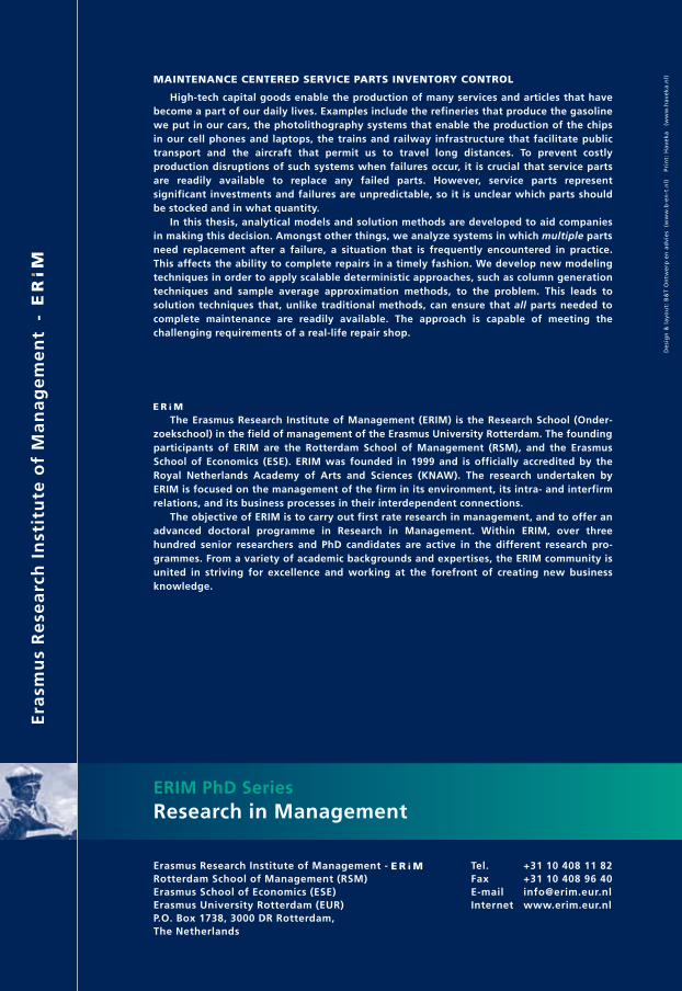
WILLEM VAN JAARSVELD
Maintenance CenteredService Parts InventoryControl
WILLE
M VAN JA
ARSVELD
- Maintenance Centered Service
Parts In
ventory Contro
l
ERIM PhD SeriesResearch in Management
Erasm
us Research Institute of Management-
288
ER
IM
De
sig
n &
la
you
t: B
&T
On
twe
rp e
n a
dvi
es
(w
ww
.b-e
n-t
.nl)
Pri
nt:
Ha
vek
a
(w
ww
.ha
vek
a.n
l)MAINTENANCE CENTERED SERVICE PARTS INVENTORY CONTROL
High-tech capital goods enable the production of many services and articles that havebecome a part of our daily lives. Examples include the refineries that produce the gasolinewe put in our cars, the photolithography systems that enable the production of the chipsin our cell phones and laptops, the trains and railway infrastructure that facilitate publictransport and the aircraft that permit us to travel long distances. To prevent costlyproduction disruptions of such systems when failures occur, it is crucial that service partsare readily available to replace any failed parts. However, service parts representsignificant investments and failures are unpredictable, so it is unclear which parts shouldbe stocked and in what quantity.
In this thesis, analytical models and solution methods are developed to aid companiesin making this decision. Amongst other things, we analyze systems in which multiple partsneed replacement after a failure, a situation that is frequently encountered in practice.This affects the ability to complete repairs in a timely fashion. We develop new modelingtechniques in order to apply scalable deterministic approaches, such as column generationtechniques and sample average approximation methods, to the problem. This leads tosolution techniques that, unlike traditional methods, can ensure that all parts needed tocomplete maintenance are readily available. The approach is capable of meeting thechallenging requirements of a real-life repair shop.
The Erasmus Research Institute of Management (ERIM) is the Research School (Onder -zoek school) in the field of management of the Erasmus University Rotterdam. The foundingparticipants of ERIM are the Rotterdam School of Management (RSM), and the ErasmusSchool of Econo mics (ESE). ERIM was founded in 1999 and is officially accre dited by theRoyal Netherlands Academy of Arts and Sciences (KNAW). The research under taken byERIM is focused on the management of the firm in its environment, its intra- and interfirmrelations, and its busi ness processes in their interdependent connections.
The objective of ERIM is to carry out first rate research in manage ment, and to offer anad vanced doctoral pro gramme in Research in Management. Within ERIM, over threehundred senior researchers and PhD candidates are active in the different research pro -grammes. From a variety of acade mic backgrounds and expertises, the ERIM commu nity isunited in striving for excellence and working at the fore front of creating new businessknowledge.
Erasmus Research Institute of Management - Rotterdam School of Management (RSM)Erasmus School of Economics (ESE)Erasmus University Rotterdam (EUR)P.O. Box 1738, 3000 DR Rotterdam, The Netherlands
Tel. +31 10 408 11 82Fax +31 10 408 96 40E-mail [email protected] www.erim.eur.nl
Mon Apr 15 2013 - B&T13181_ERIM_Omslag_Jaarsveld_15April13.pdf
Related Documents