Maintaining Robust Connectivity in Heterogeneous Robotic Networkslisc.mae.cornell.edu/LISCpapers/SPIE_CruzFierroRobustConnectivity... · Maintaining Robust Connectivity in Heterogeneous

Maintaining Robust Connectivity in Heterogeneous RoboticNetworks

P. Cruz§, R. Fierro§, W. Lu†, and S. Ferrari†

§Multi-Agent, Robotics, Hybrid and Embedded Systems (Marhes) Laboratory,Department of Electrical and Computer Engineering,University of New Mexico, Albuquerque, NM, USA;

†Laboratory of Intelligent Systems and Control (LISC),Department of Mechanical Engineering and Materials Science,

Duke University, Durham, NC, USA

ABSTRACT

In this paper, we are interested in exploiting the heterogeneity of a robotic network made of ground and aerialagents to sense multiple targets in a cluttered environment. Maintaining wireless communication on this type ofnetworks is fundamentally important specially for cooperative purposes. The proposed heterogeneous networkconsists of ground sensors, e.g., OctoRoACHes, and aerial routers, e.g., quadrotors. Adaptive potential fieldmethods are used to coordinate the ground mobile sensors. Moreover, a reward function for the aerial mobilewireless routers is formulated to guarantee communication coverage among the ground sensors and a fixedbase station. A sub-optimal controller is proposed based on an approximate control policy iteration technique.Simulation results of a case study are presented to illustrate the proposed methodology.

Keywords: Robust Connectivity, Adaptive Potential Functions, Approximate Policy Iteration, HeterogeneousSystems

1. INTRODUCTION

The scenario envisioned in this paper is intended for target sensing in hazardous environments like in a disasterarea with collapsed structures, see Figure 1(a). In these situations, the use of heterogeneous systems made upof aerial and ground robotic vehicles would maximize the probability to efficiently and successfully accomplishthe mission. For instance, aerial vehicles have the capability to cover an area faster but cannot have a detailedview of caves or buildings. On the other hand, multi-legged crawling robotic platforms can only explore alimited area, but do so with much more accuracy. In addition, a reliable wireless connectivity is an importantfactor to be considered when dealing with multi-agent systems. Due to several limitations in the communicationchannel, especially when the transmission is through the air medium, complications such as shadow effects andsecondary reflections arise. These phenomena create a variety of constrains on the possible relative positions ofthe heterogeneous agents. Thus, we are interested in developing strategies to enhance connectivity of the networkof robots and a fixed base station while a given number of targets are sensed. To be more specific, we describe atarget sensing algorithm for a ground mobile sensor network by relaxing the assumption of network connectivityintroducing a specialized aerial router agents which are better equipped to communicate over longer distances.In order to solve this problem, the mobile sensors are coordinated based on an adaptive potential method; while,Online Least-Squares Policy Iteration (online LSPI)1,2 , an Approximate Dynamic Programming (ADP) policyiteration technique, is used to modify the position of the mobile routers in order to maintain the communicationcapabilities between the sensor network and the base station.

The objective of maintaining connectivity together with additional requirements like collision avoidance orformation control in the motion planning of a multi-robot system has been extensively studied in the literature.

Further author information: (Send correspondence to P. Cruz)§ P. Cruz and R. Fierro: {pcruzec, rfierro}@ece.unm.edu† W. Lu and S. Ferrari: {wenjie.lu, sferrari}@duke.edu

Unmanned Systems Technology XV, edited by Robert E. Karlsen, Douglas W. Gage,Charles M. Shoemaker, Grant R. Gerhart, Proc. of SPIE Vol. 8741, 87410N

© 2013 SPIE · CCC code: 0277-786X/13/$18 · doi: 10.1117/12.2016236

Proc. of SPIE Vol. 8741 87410N-1

Downloaded From: http://proceedings.spiedigitallibrary.org/ on 12/09/2014 Terms of Use: http://spiedl.org/terms

9N c R3' compact Euclidean workspace,%v fixed Croatian frame,b base station,Ok convex obstacles (61,2,3),

T./ fixed targets (1=1,2),

T mobile routers (1=1,2),

S, mobile sensors (1= 1,...,6)with:

N A, platform gm meny,ni field-of-view

Snonexy(roV).

(a) (b)

Figure 1. (a) A quadrotor as communication router for a team of crawlers that are exploring and sensing a disaster area;and (b) the 3D simulation environment used in this work with a legend describing its components. The magenta vectorfrom each one of the mobile routers to the base station indicates there exists a point-to-point link between these twoelements at any time.

For instance in3 , decentralized controllers based on navigation functions for a group of robots are developedto satisfy individual sensing goals while some neighborhood connectivity relationships are maintained. In4 ,communication range and line-of-sight are used as motion constraints for a swarm of point robots which goes froman initial to a final configuration in a cluttered environment. Meanwhile,5 introduces a multi-robot explorationalgorithm that uses a utility function built taking into account the constraints of wireless networking. Monitoringthe communication link quality or the construction of a signal strength map are strategies described in6 for agood link quality maintenance in the deployment of a mobile robot network. Stochastic communication modelsare used in7 to develop an algorithm to maintain end-to-end connectivity in a team of autonomous robots.

Most of the literature on multi-agent robotic systems that considers some type of communication constraintassumes homogeneity among the members of the system. However, recent works8–11 have started exploitingthe advantage of a heterogeneous multi-robot network to enhance the communication capabilities of the wholesystem. In,8 a team of Unmanned Ground Vehicles (UGVs) performs a collaborative task while a team ofUnmanned Aerial Vehicles (UAVs) is positioned in a configuration such that they optimize the communicationlink quality to support the team of UGVs, but the authors assume that the UGVs are static to guarantee theconnectivity of the UAV-UGV network. By using a heterogeneous robotic system, a search/pursuit scenario isimplemented in9 where a control algorithm guarantees a certain level of Signal-to-Interference plus Noise Ratio(SINR) among the members of the system. Even though the field-of-view of the sensor members in the networkis considered, the geometry of the agents is neglected. The authors in10 introduce a mobile communication relayto a network of sensors and derive connectivity constraints among the network members. Afterwards, theseconstraints are used to maximize the feasible motion sets of the sensing agents. In this work as assumption, thenetwork moves in a free-obstacle environment and its agents are considered as point robots. Communicationmaintenance for a group of heterogeneous robots is enforced in11 by a passivity-based decentralized strategy.This approach allows creation/deletion of communication links at any time as long as global connectivity ispreserved, but the strategy is not tested in the case that the network has a main goal like sensing on top ofmaintaining connectivity.

Our goal is to deploy a heterogeneous system made of mobile sensors and a mobile router in an obstacle-populated area to get measurements of a number of fixed static targets. Moreover, we consider the platformand field-of-view geometry12 for the case of the sensors; while, we assume point robots only for the case of therouters. In addition, we present the 3-D environment implemented in MATLAB for simulation purposes.



. GigabyteEheet aVICON MX

m

GlgaaM 8 VICON.® § odiNI cRlO OGatlrotor GUI

Ethernet 100Mbps

Router

Station

to to will40040:46-1.'

Zig bee OctoroachModule Interface

2. BACKGROUND

In this section, we present a concise explanation about the concept of heterogeneity in robotic networks. Also, weprovide a brief overview about potential field methods and approximate dynamic programming that are behindthe implementation of the controller that will be discussed in Section 4.

2.1 Heterogeneous Robotic Networks

Heterogeneity is used in general to describe a network that consists of agents with variations on their hardwarestructure and/or on their mission objective10 . For example, hardware heterogeneity includes different sensorfootprints,13 different communication ranges10 and of course different agent dynamics9 , among many others. Onthe other hand in objective-based heterogeneity, the overall mission goal is divided into multiple sub-tasks that areassigned to each one of the agents in the network. A clear example of heterogeneity based on the mission objectiveis the dynamic sub-task coordination of an heterogeneous robotic team in the RoboCup soccer competitions14 .The difficulty in deriving suitable controllers for heterogeneous robotic networks lies in handle the hardwarevariations to combine behaviors in a way that the overall objective is achieved maintaining properties such asconvergence and stability.

The Multi-Agent Robotics Hybrid and Embedded Systems Laboratory, Marhes Lab, at the Universityof New Mexico is a clear example of an heterogeneous robotic network15 . Its robotic test-bed consists ofholonomic and non-holonomic ground vehicles, rotorcraft unmaned aerial vehicles, small crawling robots andother commercially available platforms. Figure 2(a) shows an aerial vehicle hovering over a group of legged-crawling robots in a cluttered environment. In addition, the laboratory is equipped with a high-precision motioncapture system, an up-to-date sensor suite, high-performance embedded controllers and wireless communicationdevices for networking. The block diagram in Figure 2(b) presents an example of how the test-bed is setupfrom the communications perspective. The Marhes Lab falls under both hardware-based and objective-basedheterogeneity since its robotic platforms present different agent dynamics and for example the ground robotscan be considered as mobile sensors while the aerial agents can act as communication routers dividing efforts toaccomplish a common main goal.

(a) (b)

Figure 2. The Marhes Lab, an heterogeneous robotic network: (a) a quadrotor hovering over a group of small crawlingrobots, and (b) a block diagram showing the communication links for experimental purposes.

2.2 Potential Field Methods

The potential field method is a robot motion planning approach that controls a robot movement based on thegradient field of a potential function12 . Potential field was originally developed as an on-line collision avoidanceapproach, applicable when a robot does not have a prior model of the obstacles, but senses them during motionexecution16 . The main idea besides most proposed potential functions12,16,17 is that a robot should be attracted



toward its target configuration, while being repulsed by possible obstacles. Therefore, the obstacle and targetconfiguration are considered as sources to construct a potential function U . In general, U consists of twocomponents: an attractive potential Uatt generated for example by the target configuration and a repulsivepotential Urep generated for example by the obstacles. Thus, the total potential is given by

U(x) = Uatt(x) + Urep(x),

where x = [x1 x2 ... xn]T ∈ Rn is the configuration state of the robot. The force applied on the robor isproportional to the negative gradient of U

∇U(x) =

[∂U((x))

∂x1

∂U((x))

∂x2...∂U((x))

∂xn

]T,

and it is used to design a controller for the robot movement. As in,12,16 an attractive potential can be representedas

Uatt(x) =1

2ηatt%

2t (x), (1)

where ηatt is a scaling factor and %t(x) is the Euclidean distance between the robot and the target configuration.Meanwhile, a repulsive potential can be given by

Urep(x) =

{12ηrep

(1

%o(x)− 1

d0

)2if %o(x) ≤ d0,

0 if %o(x) > d0,(2)

where ηrep is a scaling factor, %o(x) is the Euclidean distance between the robot and the nearest obstacle, anddo is the distance of influence of the obstacles. In particular, an on-line potential field method essentially actsas a descent optimization procedure, so it may get stuck at a local minimum other than the goal configuration.However, the combination of potential field methods with graph searching techniques has demonstrated to be avalid approach such that a robot escapes the local minimum12,18,19 .

2.3 Approximate Dynamic Programming

In recent years, Reinforcement Learning, RL, has grown as an effective approach for control applications andindeed many new formulations under the RL umbrella have appeared20 . RL refers to an actor, e.g., a roboticagent, which interacts with its environment and modifies its actions, e.g., its control policy, based on stimulireceived in response to its actions, e.g., a scalar reward value. Approximate Dynamic Programming, ADP, isa family of techniques within RL for the feedback control of human engineered systems21,22 . Indeed, ADP isan effective framework to circumvent the curse of dimensionality in Dynamic Programming, DP, preventing thedirect adoption of DP in many real-world control problems1,22–25 . Now, consider the discrete-time nonlineardeterministic system

xk+1 = f(xk,uk),

where k is the discrete time, x ∈ X ⊂ Rn represents the state vector of the system, u ∈ U ⊂ Rm denotes thecontrol action and f : X ×U → X is the system function. The control policy for this system is defined as afunction h : X → U such that

uk = h(xk),

and a reward function ρ : X ×U → R evaluates the immediate effect of the action uk. Indeed, it produces ascalar reward signal given by

Υk = ρ(xk, h(xk)).



f and ρ together with X and U constitute a so-called Markov Decision Process, MDP1,23 . Indeed, given f , ρ,the current state xk and the current action uk are sufficient to find the next state xk+1 and the reward Υk. Thisis the well known Markov property1,24 .

The return Q-function Q(h) : X ×U → R represents the reward obtained by the controller in the long runand it is given by

Q(h)(xk,uk) =

∞∑i=k

γi−kρ(xi,ui), (3)

where γ ∈ [0, 1) is a discount factor. In RL and DP the goal is to find an optimal policy that maximizes thereturn. Rewriting (3) as

Q(h)(xk,uk) = ρ(xk,uk) + γ

∞∑i=k+1

γi−(k+1)ρ(xi,ui),

then its equivalent difference equation is

Q(h)(xk,uk) = ρ(xk,uk) + γQ(h)(xk+1,uk+1), Q(x0,u0) = 0.

This is a nonlinear Lyapunov equation known as Bellman equation and its optimal value can be written as21

Q∗(xk,uk) = maxh

{ρ(xk,uk) + γQ(h)(xk+1,uk+1)

}.

By Bellman’s optimality principle, one gets that

Q∗(xk,uk) = maxh{ρ(xk,uk) + γQ∗(xk+1,uk+1)} .

This is the Bellman optimality equation also known as the discrte-time Hamilton-Jacobi-Bellman (HJB) equation.Then, the optimal control policy at time k is equal to

h∗(xk) = arg maxh

{ρ(xk, h(xk)) + γQ∗(xk+1, h(xk+1))} . (4)

Notice that the optimal policy at k + 1 must be known to determine the optimal policy at time k. Thus,Bellman’s principle yields by nature to offline planning methods. Also, the classical DP and RL algorithmsrequire exact representation of the value function Q(h) and the policy h. In general, this can only be achievedby storing distinct return estimates for every state-action pair. However, exact storage is not possible when thestate variables have a very large or infinite number of possibles values. Therefore, ADP is used to do onlinereinforcement learning for solving the optimal control problem by using function approximation structures toestimate the value function. In fact, online LSPI1,2 is an ADP algorithm that belongs to the approximate policyiteration (PI) techniques for ADP. In PI, the current policy is evaluated by computing its approximate valuefunction which is then used to find a new improved policy.

3. PROBLEM FORMULATION

3.1 Assumptions

In this paper we focus on a set of robots, R , made of two types of agents: L mobile sensors that form the set ofsensors S = {s1, ..., sL} and one mobile router denoted by r. Therefore, r /∈ S and R = S ∪ {r}. We divide Rin these two groups considering that the mobile sensors can be crawling robots, i.e., OctoRoACHes26 , while thecommunication relays can be unmanned aerial vehicles, i.e., quadrotors27 .

The set R operates in W ⊂ R3 which is a compact subset of a three-dimensional Euclidean space where thereis a fixed base station b . In R , there are M convex obstacles grouped in the set O = {O1, ...,OM} and there areN static rigid targets that forms the set T = {T1, ...,TN} such that O ∩ T = ∅. We denote IO and IT as the



index sets of O and T , respectively. For all j ∈ IT , we call oT j to the center of Tj . Meanwhile embedded in W ,there is a fixed Cartesian frame FW with origin oW . FW allows us to describe the position and orientation ofthe agents, objects and targets in W . For instance, ∀k ∈ IO , every point of Ok has a fixed position with respectto FW because the Ok’s are considered rigid and fixed in W 16 . Figure 1(b) shows the 3D environment createdin MATLAB for simulation purposes. Also, we include in this figure a legend on the right top corner to facilitatethe reference of the different elements consider in this paper.

3.1.1 Motion Dynamics

Let IS be the index set of S , then IS = {1, ..., L}. We consider ∀i ∈ IS si has a platform geometry Ai ⊂ R3 anda field-of-view (FOV) geometry Vi ⊂ R3 from which the robot can obtain sensor measurements12,28 , see Figure1(b). We also assume Ai = Aj and Vi = Vj ∀i, j ∈ IS . Furthermore, Ai and Vi are both rigid and Vi has a fixed

position and orientation with respect to Ai. We say that ∀i ∈ IS and ∀j ∈ IT the sensor si gets measurements

of the target Tj when Vi ∩ Tj 6= ∅. In fact, we ensure this last condition when si ∈ B(

oTj , dosens

)where dosens

is the minimum distance to the target Tj for getting measurements. We use B(q, δ) to denote the open ball ofradius δ centered at q. In addition, we suppose that FA i is a Cartesian frame embedded in Ai with origin oA i.Now let (xsi , ysi) be the position of FA i respect to FW and let θi be the orientation of FA i respect to FW . Then,we define ∀i ∈ IS the state vector of the sensor si as qsi = [xsi ysi θi] ∈ SE(2). In other words, we consider thatevery si is moving just on the xy plane with θi as its heading angle. Notice that qsi can be used to determinethe position and orientation of Ai and Vi respect to FW . The state vector of each mobile sensor, qsi , must alsosatisfy the sensor dynamics that are given by the unicycle model,

xsi = vi cos θi,ysi = vi sin θi,vi = ai,

θi = ωi,

(5)

where ai and ωi are the ith mobile sensor’s linear acceleration and angular velocity, respectively. Thus, thecontrol vector for the si sensor is usi = [ai ωi] ∈ R2.

On the other hand for the mobile router r, the range of communication coverage is denoted as δr. We alsoassume that r moves at a safe fixed height over the mobile sensors and over all the obstacles in W . Furthermore,its motion dynamics are given by

qr = ur, (6)

where qr = [xr yr zr] ∈ R3 is the state vector of the mobile router and specifies its 3-D position respect to FW ,while ur ∈ R3 is its acceleration control input. We say that ur = h(qr) where h(·) is the control policy for r.

3.1.2 Communication Links

For the next definitions, q(xy) = q · vxy where vxy = [1 1 0]T . In our scenario, see Figures 3(a) and 3(b), weassume there is a point-to-point link between the mobile router r and the base station b at any time. This linkis represented by the magenta vector in Figures 3(a) and 3(b). Also, we suppose that r can manage at any timecommunication packets between any pair of sensors in S or between a sensor in S and b . Indeed, we introducethe next two definitions.

Definition 3.1. For all i, j ∈ IS , i 6= j, si has bidirectional communication with sj if q(xy)si ,q

(xy)sj ∈ B

(q(xy)r , δr

).

Definition 3.2. For every i ∈ IS , si has bidirectional communication with b if q(xy)si ∈ B

(q(xy)r , δr

).

Therefore, a mobile sensors can talk with one of its pairs just if both are within the ball of radius δr and

centered at q(xy)r . Similarly, a mobile sensor can receive/send information from/to the base station just if it is

within the ball of radius δr and centered at q(xy)r . It is clear if Definition 3.2 holds for every i ∈ IS then Definition

3.1 also holds. Consequently, we can combine both definitions as next



6

a

o^r

-15 °

Definition 3.3. If ∀i ∈ IS ,q(xy)si ∈ B

(q(xy)r , δr

)then si has bidirectional communication with any sj where

j ∈ IS , i 6= j, and si also has bidirectional communication with b.

Considering the explanation on Section 2.1 and from the assumptions detailed in Sections 3.1.1 and 3.1.2,R is an heterogeneous robotic network that exhibits hardware-based and objective-based heterogeneity. In fact,we are assuming agents with different dynamics and communication ranges, so R has hardware heterogeneity.Also, R presents objective-based heterogeneity because we assume that the ground agents objective is purelytarget sensing while the aerial agent objective is maintaining connectivity among the mobile sensors and the basestation.

(a) (b)

Figure 3. Representation of the communication constraints specified by Definitios 3.1, 3.2 and 3.3. (a) 3D-view, and (b)2D-view (xy view).

3.2 Problem Statement

Under the assumptions described in 3.1, we are concerned with the following problem: A set of heterogeneousrobots R formed by L mobile sensors and one mobile router r must obtain measurements of M targets locatedin an obstacle populated environment such that R maintains inter-agent connectivity and also connectivity witha base station b .

Since the set R works in a cluttered scenario, we have to add inter-robot collision prevention and obstacleavoidance to the objectives stated in the problem. Consequently, the problem considered in this paper aims todesign a controller for the agents of the heterogeneous robotic network R such that they: (i) sense M statictargets, (ii) keep inter-agent connectivity among the mobile sensors, (iii) keep mobile sensor and base stationconnectivity, (iv) avoid inter-agent collisions, and (v) avoid obstacle collisions. From the assumptions given inSection 3.1, the objectives (i) to (v) need to be considered for the design of the controller for the mobile sensors.On the contrary, the objectives (i), (iv) and (v) are not part of the controller design for the mobile router rbecause we assume that it has only communication and not sensing capabilities, and it always flies at a safeheight over the mobile sensors and obstacles. In the next section, the proposed controllers for the mobile sensorsand for the mobile router are described.



4. METHODOLOGY

From the problem statement, Section 3.2, we need to design two local controllers: one for the mobile sensors andone for the mobile router. Next, we present the methodologies around these controllers and then they will betested in simulation, see Section 5. For the next definitions, ‖ · ‖ denotes the Euclidean norm.

4.1 Mobile Sensor Controller

In this case, the objectives (i) to (v) have to be accomplished by the controller of each si ∈ S . For thesensing objective (i), we consider that the set of mobile sensors S takes measurements of the M targets inT = {T1, ...,TM} in sequential order. This is first take measurements of T1 then of T2 and so on until S takesmeasurements of TM . For each si, we design its controller based on potential field methods, Section 2.2, andspecially taking as a based the potential functions given in equation (1), an attractive potential, and in equation(2), a repulsive potential. Thus, we define Ui(qsi), the potential function of the ith mobile sensor with i ∈ IS as

Ui(qsi) = Ut(qsi) + Uc(qsi) + Uo(qsi), (7)

where Ut(qsi) is the attractive potential of the jth target with j ∈ IT , Uc(qsi) is a combination of an attractivepotential for keeping inter-sensor connectivity and a repulsive potential for avoiding inter-sensor collision, andUo(qsi) is a repulsive potential for obstacle avoidance.

The attractive potential Ut(qsi) is given by

Ut(qsi) =

{12ηt%

2t (qsi ,Tj) if %t(qsi ,Tj) ≥ dosens ,

0 if %t(qsi ,Tj) < dosens ,(8)

where dosens is the required distance from si to Tj to get sensor measurements, see Section 3.1.1, and %t(qsi ,Tj)is the distance between the mobile sensor si and the target Tj defined as

%t(qsi ,Tj) = max{‖q(xy)

si − o(xy)1 ‖, ‖q(xy)

si − o(xy)2 ‖

},

with o1,o2 ∈ Tj , i.e., o1 and o2 are the coordinates of two points within Tj .The potential Uc(qsi) is defined as

Uc(qsi) =

L∑l=1,l 6=i

U(qsi ,qsl), (9)

with

U(qsi ,qsl) =

12ηc%

2s(qsi ,qsl) if %s(qsi ,qsl) >

δr2 ,

12ηc

(1

%s(qsi,qsl

) −1

docol

)2if %s(qsi ,qsl) ≤ docol ,

0 otherwise,

(10)

where δr > docol , δr is the range of communication coverage, see Section 3.1.1, docol is the clearance inter-sensor

distance, and %s(qsi ,qsl) = ‖q(xy)si − q

(xy)sl ‖.

The repulsive potential for obstacle avoidance Uo(qsi) is given by

Uo(qsi) =

M∑k=1

U(qsi ,Ok), (11)

with

U(qsi ,Ok) =

{12ηrep

(1

%o(qsi,Ok)− 1

doobj

)2if %o(qsi) ≤ doobj ,

0 if %o(qsi) > doobj ,(12)



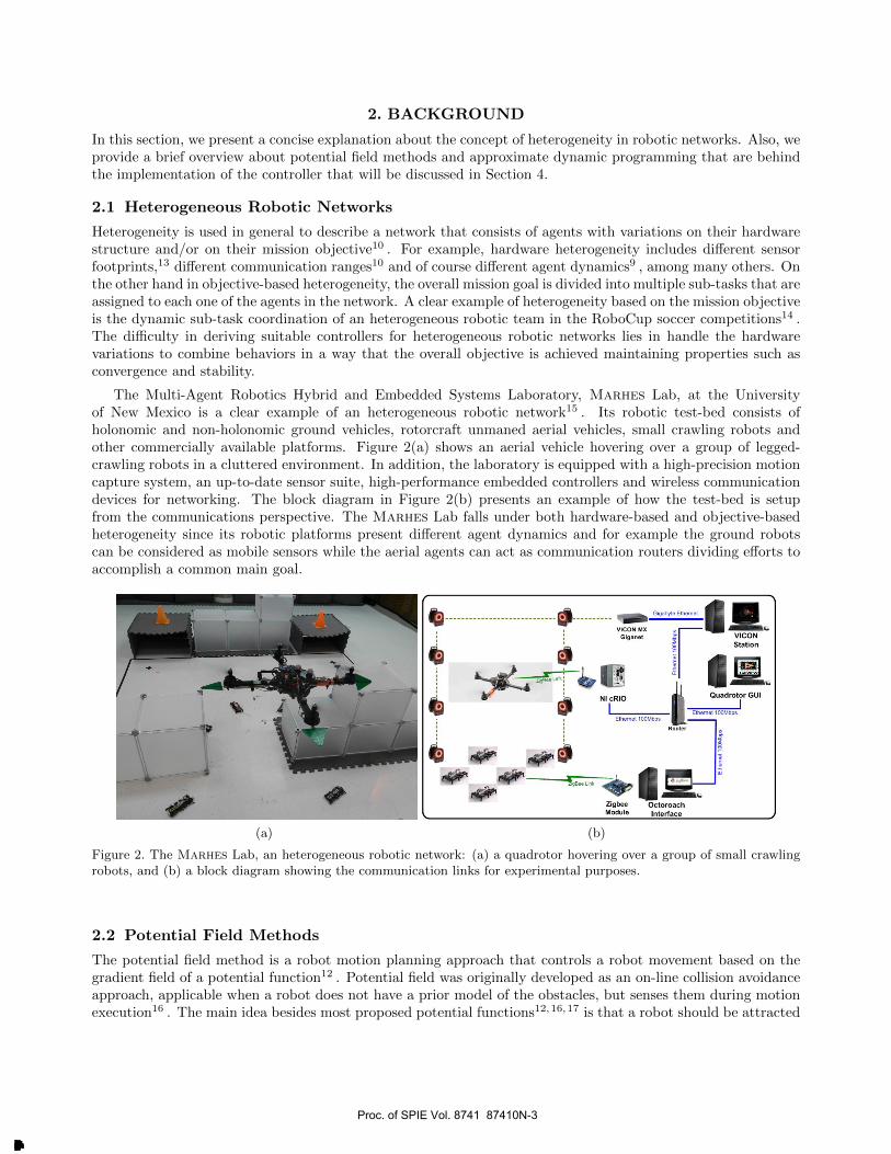
where %o(qsi ,Ok) is the distance between si and the kth obstacle, and doobj is the influence distance of theobstacles.

Respect to the scaling factors ηt, ηc, and ηo, we assign their values according to Algorithm 1. Using thisalgorithm, we adapt the relative importance of the potential functions Ut(qsi), U(qsi ,qsl), and U(qsi ,Ok)between each other at every step time. For example, if a mobile sensor si is far from a target, but it is morepossible a inter-sensor collision than an obstacle collision, i.e., ec > eo > et, then we give more priority to thepotential function U(qsi ,qsl) with Algorithm 1 in order to avoid the inter-sensor collision.

Algorithm 1 Assignment of the scaling factors ηt, ηc and ηoInput: : β1, β2, and β3 positive scaling factors such that β1 > β2 > β3

1: et =

{|%t(qsi ,Tj)− dosens

| if %t(qsi ,Tj) ≥ dosens

0 if %t(qsi ,Tj) < dosens

2: ec =

|%s(qsi ,qsl)−δr2 | if %s(qsi ,qsl) >

δr2

|%s(qsi ,qsl)− docol | if %s(qsi ,qsl) ≤ docol0 otherwise

3: eo =

{|%o(qsi)− doobj | if %o(x) ≤ doobj0 if %o(qsi) > doobj

4: if et ≥ ec and et ≥ eo then5: ηt = β16: if ec ≥ eo then7: ηc = β2, ηo = β38: else9: ηc = β3, ηo = β2

10: end if11: else if et < ec and et ≥ eo then12: ηt = β2, ηc = β1, ηo = β313: else if et ≥ ec and et < eo then14: ηt = β2, ηc = β3, ηo = β115: else16: ηt = β317: if ec ≥ eo then18: ηc = β1, ηo = β219: else20: ηc = β2, ηo = β121: end if22: end if

The gradient of Ui(qsi) is

∇Ui(qsi) =

[∂Ui(qsi)

∂xsi

∂Ui(qsi)

∂ysi

∂Ui(qsi)

∂θi

],

and then the artificial force induced by the potential function is Fi(qsi) = −∇Ui(qsi). Now from Section 3.1.1,the control vector for the si sensor is usi = [ai ωi], so the potential-based control law29 is given by

ai = −[cos θi sin θi 0]∇Ui(qsi)T − k0vi, (13)

ωi = k1

[atan2

(∂Ui(qsi)

∂xsi,∂Ui(qsi)

∂ysi

)− θi

], (14)

where k0 and k1 are positive constants.



4.2 Mobile Router Controller

The mobile router controller must satisfy the objectives (ii) and (iii) enumerated in Section 3.2. Indeed, theseobjectives are satisfied if Definition 3.3 holds. Thus, the mobile router r needs to maintain an adequate relativeposition respect to each one of the mobile sensors in S . We formulate the next reward function for r in order toensure its adequate position at all times,

ρc(qr) =

L∑i=1

ζ(e−%r(qr,qsi

)/τ), (15)

where ζ is a positive scaling parameter, 0 < τ � 1, and %r(qr,qsi) is the separation distance given by

%r(qr,qsi) = |‖q(xy)r − q(xy)

si ‖ − δr|. (16)

In addition, a reward function ρr(ur) is associated with the control input for the relay such that

ρr(ur) = uTr Rrur, (17)

where Rr = diag[a b c] with scalar weights a, b, c > 0. Considering the rewards (15) and (17), the total termfunction for the mobile router is

Υ(qr,ur) = ρc(qr)− ρr(ur), (18)

and using this function, we create the Q-function for the router as

Q(h)(qr,ur) =

∞∑k=0

γkΥ(qr(k),ur(k)), (19)

where γ ∈ [0, 1) is the discount factor. Therefore, our goal is to select the control policies h(qr) such thatQ(qr,ur) is maximized.

Online LSPI algorithm1,2 is used to solve this optimal control problem. This algorithm is an approximate PItechnique for ADP (see Section 2.3). In general, the PI algorithm starts with an arbitrary initial policy h0. Thenat every iteration ` ≥ 0, it evaluates the current policy, i.e., compute its Q-function Qh` and finds an improvedpolicy using

h`+1(qr) = arg maxh{Q(h`)(qr,ur)} (20)

The PI algorithm converges to an optimal policy h∗23 . In online LSPI, the Q function is approximated usingthe linear parametrization

Q(qr,ur) = φT (qr,ur)θ (21)

where φ(qr,ur) = [φ1(qr ur) ... φm(qr,ur)]T

is a vector of m basis functions, BFs, and θ ∈ Rm is a parametervector. In order to find the approximate Q-function of the current policy, online LSPI computes the parametervector from a batch of samples running least-squares temporal difference for Q-functions, LSTD-Q,24,30 that isa policy evaluation algorithm. Considering a set of samples

{(qrls ,urls ),Υ(qrls ,urls )|ls = 0, ..., ns

}constructed

by state-action samples and then computing next states and rewards, LSTD-Q process the samples using

Γls+1 = Γls + φ(qrls ,urls )φT (qrls ,urls )

Λls+1 = Λls + φ(qrls ,urls )φT (qrls+1,urls+1

) (22)

zls+1 = zls + φ(qrls ,urls )ρ(qrls ,urls )

with Γ0 = 0,Λ0 = 0, z0 = 0, and then solves the equation

1

nsΓns

θh = γ1

nsΛns

θh +1

nszns

(23)



to find an approximate parameter vector θh. The solution θh found by LSTD-Q is substitute in (21) to getan approximate Q-function which is used to perform a policy improvement with (20) obtaining in this way anapproximate PI algorithm. Indeed, online LSPI performs policy improvements once every few transitions beforean evaluation of the current policy can be completed. Thus by exploiting the data collected by interaction, theonline LSPI algorithm provides policy improvements. Furthermore, it explores other actions than those given bythe current policy. In fact, the classical ε-greedy exploration24 is used at every step k.

Algorithm 2 Online LSPI with ε-greedy exploration

Input: : discount factor γ, BFs φ1, ...,φn, a small constant βΓ > 0policy improvement interval Kθ, exploration schedule {εk}∞k=0

1: ` = 0, initialize policy h02: Γ0 = βΓIn×n,Λ0 = 0, z0 = 03: measure initial state x0

4: for every time step k = 0, 1, 2, ... do

5: urk =

{h`(qrk) with probability 1− εk (exploit)a uniform random action with probability εk (explore)

6: apply urk , measure next state qrk+1and reward Υk+1

7: Γk+1 = Γk + φ(qrk ,urk)φT (qrk ,urk)8: Λk+1 = Λk + φ(qrk ,urk)φT (qrk+1

,urk+1)

9: zk+1 = zk + φ(qrk ,urk)ρ(qrk ,urk)10: if k = (`+ 1)Kθ then11: solve 1

k+1Γk+1θ` = γ 1k+1Λk+1θ` + 1

k+1zk+1 B finalize policy evaluation

12: h`+1(x) = arg maxh{φT (qr,ur)θ`} B policy improvement13: ` = `+ 114: end if15: end for

Algorithm 2 presents the online LSPI with ε-greedy exploration approach1,2 applied for our case. The numberKθ ∈ N,Kθ 6= 0 is the number of transitions between consecutive policy improvements. When Kθ = 1 the policyis updated after every sample and the online LSPI is fully optimistic23 . Meanwhile, the algorithm is partiallyoptimistic when Kθ > 1. In general, the number Kθ should not be chosen too large. About the explorationschedule {εk}∞k=0, it should not approach to zero fast since a significant amount of exploration is recommended.

5. SIMULATION RESULTS

A 3-D environment is developed in MATLAB to test the methods proposed in Section 4. The sensor platformgeometry as well as its FOV geometry are shown in Figure 1(b). On the other hand, the mobile routers areassumed as point robots, but they are represented as a thin cross with four circles at each side just for visualizationpurposes, see Figure 1(b) and Figure 4. Obstacle geometries and target geometries are assumed to be known apriori. The heterogeneous network considered for simulation is formed by 1 mobile router and 3 mobile sensors.The network moves in an environment W of 4×4×1.5 m3 with 4 obstacles and 2 targets, see Figure 4. The basestation is located at the position (−1.75, 1.75) m closed where the network starts moving to. The communicationcoverage radius for the mobile router is δr = 1 m. The time dynamics, equation (5) for the sensors and equation(6) for the router, are implemented at each time step using ode45-differential equation solver in MATLAB. Thestep time is set up at 0.01 sec.

For the simulation, just the methodology proposed for the mobile sensors, Section 4.1, and Algorithm 1 arecompletely developed. We are currently working on the implementation of the sub-optimal controller for themobile router. Therefore as initial test, we consider also a potential function control approach for the routerwhere the potential function is given by

Ur(qr) =

L∑i=1

U(qr,qsi), (24)



where

U(qr,qsi) =

{12ηr%

2rs(qr,qsi) if %rs(qr,qsi) ≥ δr

2 ,

0 if %rs(qr,qsl) <δr2 ,

(25)

with %rs(qr,qsi) = ‖q(xy)r − q

(xy)si ‖. Thus, the controller law is defined as

ur = −k3[∂Ur(qr)

∂xr

∂Ur(qr)

∂yr0

]T+ k4ur, (26)

where k3 and k4 are positive constants.

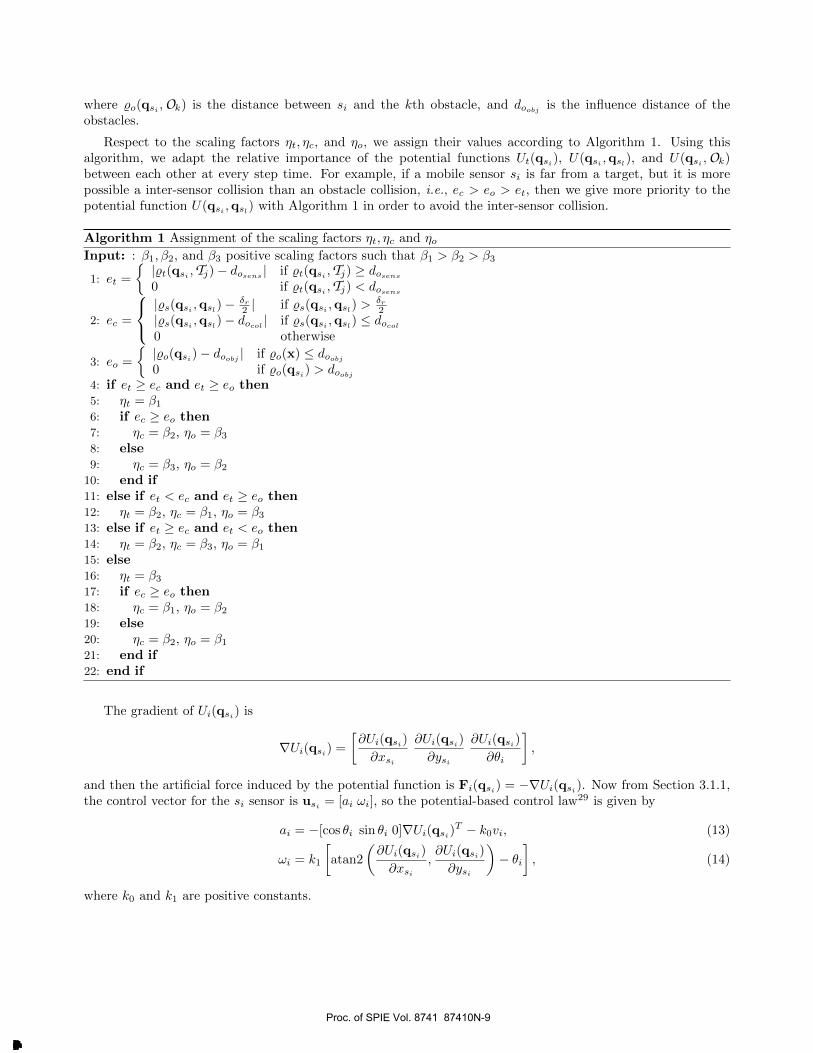
For Algorithm 1, we select β1 = 0.295, β2 = 0.125, and β3 = 0.105, and for the sensors control law, equations(13) and (14), we set k0 = k1 = 0.75. In the case of the mobile router controller, equation (26), k3 = 0.95 andk4 = 0.85 and in equation (25) ηr = 0.425. Figure 4 presents the 3-D view (parts (a) and (c)) and 2-D view(parts (b) and (d)) at two different time instants during the simulation. After 35 seconds, Figures 4(a) and 4(b),the heterogeneous network arrives to the first target and it is on its way to the second target at time equal to40 seconds, Figures 4(c) and (d).

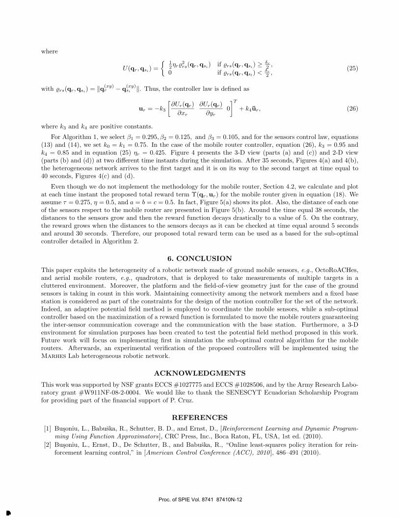
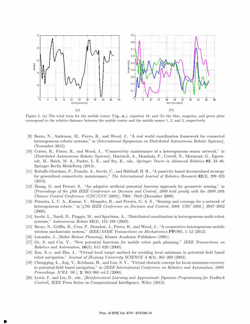
Even though we do not implement the methodology for the mobile router, Section 4.2, we calculate and plotat each time instant the proposed total reward term Υ(qr,ur) for the mobile router given in equation (18). Weassume τ = 0.275, η = 0.5, and a = b = c = 0.5. In fact, Figure 5(a) shows its plot. Also, the distance of each oneof the sensors respect to the mobile router are presented in Figure 5(b). Around the time equal 38 seconds, thedistances to the sensors grow and then the reward function decays drastically to a value of 5. On the contrary,the reward grows when the distances to the sensors decays as it can be checked at time equal around 5 secondsand around 30 seconds. Therefore, our proposed total reward term can be used as a based for the sub-optimalcontroller detailed in Algorithm 2.

6. CONCLUSION

This paper exploits the heterogeneity of a robotic network made of ground mobile sensors, e.g., OctoRoACHes,and aerial mobile routers, e.g., quadrotors, that is deployed to take measurements of multiple targets in acluttered environment. Moreover, the platform and the field-of-view geometry just for the case of the groundsensors is taking in count in this work. Maintaining connectivity among the network members and a fixed basestation is considered as part of the constraints for the design of the motion controller for the set of the network.Indeed, an adaptive potential field method is employed to coordinate the mobile sensors, while a sub-optimalcontroller based on the maximization of a reward function is formulated to move the mobile routers guaranteeingthe inter-sensor communication coverage and the communication with the base station. Furthermore, a 3-Denvironment for simulation purposes has been created to test the potential field method proposed in this work.Future work will focus on implementing first in simulation the sub-optimal control algorithm for the mobilerouters. Afterwards, an experimental verification of the proposed controllers will be implemented using theMarhes Lab heterogeneous robotic network.

ACKNOWLEDGMENTS

This work was supported by NSF grants ECCS #1027775 and ECCS #1028506, and by the Army Research Labo-ratory grant #W911NF-08-2-0004. We would like to thank the SENESCYT Ecuadorian Scholarship Programfor providing part of the financial support of P. Cruz.

REFERENCES

[1] Busoniu, L., Babuska, R., Schutter, B. D., and Ernst, D., [Reinforcement Learning and Dynamic Program-ming Using Function Approximators ], CRC Press, Inc., Boca Raton, FL, USA, 1st ed. (2010).

[2] Busoniu, L., Ernst, D., De Schutter, B., and Babuska, R., “Online least-squares policy iteration for rein-forcement learning control,” in [American Control Conference (ACC), 2010 ], 486–491 (2010).



YX

Y ,m,X ,m,

[w] A

(a) (b)

(c) (d)

Figure 4. 3-D environment with 4 obstacles, 5 targets, 1 mobile router, and 3 mobile sensors. At two different timeinstants a 3-D view, (a) and (c), and a 2-D view, (b) and (d), are presented in this figure.

[3] Pereira, G. A. S., Das, A. K., Kumar, V., and Campos, M. F. M., “Decentralized motion planning formultiple robots subject to sensing and communication constraints,” in [Proceedings of the Second MultiRobotSystems Workshop ], 267–278, Kluwer Academic Press (2003).

[4] Esposito, J. and Dunbar, T., “Maintaining wireless connectivity constraints for swarms in the presence ofobstacles,” in [IEEE International Conference on Robotics and Automation (ICRA), 2006 ], 946 – 951 (May2006).

[5] Rooker, M. N. and Birk, A., “Multi-robot exploration under the constraints of wireless networking,” ControlEngineering Practice 15(4), 435–445 (2007).

[6] Hsieh, M. A., Cowley, A., Kumar, V., and Taylor, C. J., “Maintaining network connectivity and performancein robot teams,” Journal of Field Robotics 25(1-2), 111–131 (2008).

[7] Fink, J., Ribeiro, A., and Kumar, V., “Motion planning for robust wireless networking,” in [IEEE Interna-tional Conference on Robotics and Automation (ICRA), 2012 ], 2419–2426 (2012).

[8] Gil, S., Schwager, M., Julian, B. J., and Rus, D., “Optimizing communication in air-ground robot networksusing decentralized control,” in [IEEE International Conference on Robotics and Automation (ICRA), 2010 ],1964–1971 (2010).



(spuooas] auaiL

09 SV OP S£ 0£ 9Z OZ SL OL

1

t

OL

SL

ú OZ

9Z

0£

[spuooas] auaiL

09 9V OP SC OC 9Z OZ 9L OL

L'0

Z'0

CO '

P.O

9'0

9'0

L'0

8'0

6'0

(a) (b)

Figure 5. (a) The total term for the mobile router Υ(qr,ur), equation 18, and (b) the blue, magenta, and green plotscorrespond to the relative distance between the mobile router and the mobile sensor 1, 2, and 3, respectively.

[9] Bezzo, N., Anderson, M., Fierro, R., and Wood, J., “A real world coordination framework for connectedheterogeneous robotic systems,” in [International Symposium on Distributed Autonomous Robotic Systems ],(November 2012).

[10] Cortez, R., Fierro, R., and Wood, J., “Connectivity maintenance of a heterogeneous sensor network,” in[Distributed Autonomous Robotic Systems ], Martinoli, A., Mondada, F., Correll, N., Mermoud, G., Egerst-edt, M., Hsieh, M. A., Parker, L. E., and Sty, K., eds., Springer Tracts in Advanced Robotics 83, 33–46,Springer Berlin Heidelberg (2013).

[11] Robuffo Giordano, P., Franchi, A., Secchi, C., and Bulthoff, H. H., “A passivity-based decentralized strategyfor generalized connectivity maintenance,” The International Journal of Robotics Research 32(3), 299–323(2013).

[12] Zhang, G. and Ferrari, S., “An adaptive artificial potential function approach for geometric sensing,” in[Proceedings of the 48th IEEE Conference on Decision and Control, 2009 held jointly with the 2009 28thChinese Control Conference (CDC/CCC 2009) ], 7903 –7910 (December 2009).

[13] Pimenta, L. C. A., Kumar, V., Mesquita, R., and Pereira, G. A. S., “Sensing and coverage for a network ofheterogeneous robots,” in [47th IEEE Conference on Decision and Control, 2008. CDC 2008. ], 3947–3952(2008).

[14] Iocchi, L., Nardi, D., Piaggio, M., and Sgorbissa, A., “Distributed coordination in heterogeneous multi-robotsystems,” Autonomous Robots 15(2), 155–168 (2003).

[15] Bezzo, N., Griffin, B., Cruz, P., Donahue, J., Fierro, R., and Wood, J., “A cooperative heterogeneous mobilewireless mechatronic system,” IEEE/ASME Transactions on Mechatronics PP(99), 1–12 (2012).

[16] Latombe, J., [Robot Motion Planning ], Kluwer Academic Publishers (1991).

[17] Ge, S. and Cui, Y., “New potential functions for mobile robot path planning,” IEEE Transactions onRobotics and Automation, 16(5), 615–620 (2000).

[18] Zou, X.-y. and Zhu, J., “Virtual local target method for avoiding local minimum in potential field basedrobot navigation,” Journal of Zhejiang University SCIENCE A 4(3), 264–269 (2003).

[19] Chengqing, L., Ang, V., Krishnan, H., and Lim, S. Y., “Virtual obstacle concept for local-minimum-recoveryin potential-field based navigation,” in [IEEE International Conference on Robotics and Automation, 2000.Proceedings. ICRA ’00. ], 2, 983–988 vol.2 (2000).

[20] Lewis, F. and Liu, D., eds., [Reinforcement Learning and Approximate Dynamic Programming for FeedbackControl ], IEEE Press Series on Computational Intelligence, Wiley (2012).



[21] Lewis, F. and Vrabie, D., “Reinforcement learning and adaptive dynamic programming for feedback control,”IEEE Circuits and Systems Magazine 9(3), 32–50 (2009).

[22] Si, J., Barto, A. G., Powell, W. B., and Wunsch, D., [Handbook of Learning and Approximate DynamicProgramming ], IEEE Press Series on Computational Intelligence, Wiley-IEEE Press (2004).

[23] Bertsekas, D. P., [Dynamic Programming and Optimal Control, Vol. I and Vol. II ], Athena Scientific, 3rd(Vol. I) and 4th (Vol. II) ed. (2005 (Vol. I) and 2012 (Vol. II)).

[24] Powell, W. B., [Approximate Dynamic Programming: Solving the Curses of Dimensionality ], Wiley Seriesin Probability and Statistics, Wiley-Interscience (2007).

[25] Wang, F.-Y., Zhang, H., and Liu, D., “Adaptive dynamic programming: An introduction,” IEEE Compu-tational Intelligence Magazine 4(2), 39–47 (2009).

[26] Pullin, A., Kohut, N., Zarrouk, D., and Fearing, R., “Dynamic turning of 13 cm robot comparing tail anddifferential drive,” in [2012 IEEE International Conference on Robotics and Automation (ICRA) ], 5086–5093 (May 2012).

[27] Bouabdallah, S. and Siegwart, R., Design and control of quadrotors with application to autonomous flying,These sciences, Faculte des sciences et techniques de l’ingenieur STI, Section de microtechnique, Institutd’ingenierie des systemes I2S (Laboratoire de systemes autonomes 1 LSA1). Dir.: Roland Siegwart, Ecolepolytechnique federale de Lausanne, EPFL, Lausanne (2007).

[28] Ferrari, S., Anderson, M., Fierro, R., and Lu, W., “Cooperative navigation for heterogeneous autonomousvehicles via approximate dynamic programming,” in [2011 50th IEEE Conference on Decision and Controland European Control Conference (CDC-ECC) ], 121–127 (2011).

[29] Ferrari, S., Fierro, R., and Wettergren, T., [Modeling and Control of Dynamic Sensor Networks ], CRCPress, Inc. (2013). (To be published).

[30] Lagoudakis, M. G., Parr, R., and Littman, M. L., “Least-squares methods in reinforcement learning forcontrol,” in [SETN 02: Proceedings of the Second Hellenic Conference on AI ], 249–260, Springer-Verlag(2002).



Maintaining Robust Connectivity in Heterogeneous Robotic Networkslisc.mae.cornell.edu/LISCpapers/SPIE_CruzFierroRobustConnectivity... · Maintaining Robust Connectivity in Heterogeneous

Documents