Magnetic Monopoles Magnetic Monopoles Roman Schmitz Seminar on Theoretical Particle Physics University of Bonn May 4th 2006

Welcome message from author
This document is posted to help you gain knowledge. Please leave a comment to let me know what you think about it! Share it to your friends and learn new things together.
Transcript

Magnetic Monopoles
Magnetic Monopoles
Roman Schmitz
Seminar on Theoretical Particle PhysicsUniversity of Bonn
May 4th 2006

Magnetic Monopoles
Overview
Introduction
Dirac MonopolesMaxwell’s Equations and DualityThe magnetic monopole fieldDirac’s Quantization of Magnetic ChargeSummary
’t Hooft-Polyakov MonopolesWhat are Solitons ?Solitons in the SO(3) model’t Hooft Polyakov SolitonThe ’t Hooft-Polyakov-Monopole

Magnetic Monopoles
Introduction
Motivation: Why magnetic monopoles ?
I First idea from Dirac in 1931 (symmetric form ofMaxwell-Equations)
I Appear in non-abelian gauge theories with symmetrybreakdown
I possibly particles not yet observed, no experimental evidenceup to now!

Magnetic Monopoles
Dirac Monopoles
Maxwell’s Equations
The Maxwell Equations in terms of the Dual Tensor
Take Maxwell Equations:
∂νFµν = −jµ dF = 0
In terms of the Dual Tensor defined as
Fµν =1
2εµνρσFρσ
with components:
F 0i =1
2ε0ijkFjk = −1
2ε0ijkεjklB
l = B i
F ik =1
2εijµνFµν =
1
2(εijk0Fk0 + εij0lF0l = e ijkE k)
Maxwell’s equations read:
∂νFµν = −jµ ∂ν F
µν = 0

Magnetic Monopoles
Dirac Monopoles
Maxwell’s Equations
Extension of Maxwell’s Equations
To describe Monopoles construct a magnetic 4-current in analogyto the electrical:
kµ = (σ,~k)
Now Maxwell’s Equations read
∂νFµν = −jµ ∂ν F
µν = −kµ
in a nice symmetric form and are invariant under the so-calledDuality Transformation:
Fµν 7→ Fµν Fµν 7→ −Fµν jµ 7→ kµ kµ 7→ −jµ

Magnetic Monopoles
Dirac Monopoles
The magnetic monopole field
Magnetic monopole field
Magnetic field for a point-source with magnetic charge g:
~B(~r , t) =g
4πr2·~r
r
Problem:
div ~B = ~∇ · g
4π·
~r
r3︸︷︷︸=~∇(− 1
r)
= − g
4π∆
1
r= − g
4πδ(r) 6= 0
⇒ @~A s.t. ~B = rot~A
Is this the end of magnetic monopoles ?

Magnetic Monopoles
Dirac Monopoles
The magnetic monopole field
Solution: The Dirac string
Add an infinetely small, infinitely extended solenoid field (e.g.along the negative z-axis):
~Bsol =g
4πr2r + g ·Θ(−z)δ(x)δ(y)z
Verify that the flux is zero by integrating and using Gauss’theorem. Now:
~BMonopole = rot~Asol − g ·Θ(−z)δ(x)δ(y)z

Magnetic Monopoles
Dirac Monopoles
Quantization
Dirac’s Quantization of Magnetic Charge
Motion of charged particle in Monopole field:
d
dtL = m[~r × ~r ] =
gq
4πr3[~r × [~r ×~r ]] =
gq
4π(~r
r−~r(~r ·~r)
r3)︸ ︷︷ ︸
= ddt
~rr
=d
dt
gq~r
4πr
Angular momentum of Electromagnetic field:
LEM =
Zd3x[~r × [~E × ~B]] =
Zd3x
~E
r−
~r
r3(~r · ~E) =
Zd3xE i (∇i r) = −
gq~r
4πr
In QM quantized angular momenta in units of n2 :
eg
4π=
n
2
Magnetic Monopoles
Dirac Monopoles
Quantization
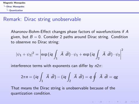
Remark: Dirac string unobservable
Aharonov-Bohm-Effect changes phase factors of wavefunctions if Agiven, but B = 0. Consider 2 paths around Dirac string. Conditionto obsereve no Dirac string:
|ψ1 + ψ2|2 =
∣∣∣∣exp (iq
∫1
~A ~dl) · ψ1 + exp (iq
∫2
~A ~dl) · ψ2
∣∣∣∣2interference terms with exponents can differ by n2π:
2πn = (iq
∫1
~A ~dl)− (iq
∫2
~A ~dl) = q
∮~A ~dl = qg
That means the Dirac string is unobservable because of thequantization condition.
Magnetic Monopoles
Dirac Monopoles
Quantization
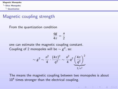
Magnetic coupling strength
From the quantization condition
qg
4π=
n
2
one can estimate the magnetic coupling constant.Coupling of 2 monopoles will be ∼ g2, so:
∼ g2 ∼ n2
4· (4π)2
q2∼ n2
4q2
(4π
q2
)2
︸ ︷︷ ︸1/α2
The means the magnetic coupling between two monopoles is about104 times stronger than the electrical coupling.
Magnetic Monopoles
Dirac Monopoles
Quantization
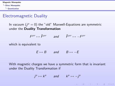
Electromagnetic Duality
In vacuum (jµ = 0) the ”old” Maxwell-Equations are symmetricunder the Duality Transformation
Fµν 7→ Fµν and Fµν 7→ −Fµν
which is equivalent to
E 7→ B and B 7→ −E
With magnetic charges we have a symmetric form that is invariantunder the Duality Transformation if
jµ 7→ kµ and kµ 7→ −jµ
Magnetic Monopoles
Dirac Monopoles
Summary
Summary
I symmtreic form of Maxwell Equations, duality transformation
I describes quantization of electric/magnetic charges by QM
I still have to deal with point-sources and singularities
I Dirac string unobservable
I no mass predictions

Magnetic Monopoles
’t Hooft-Polyakov Monopoles
Solitons
What are Solitons ?
Solitary waves or so-called Solitons are static finite-energy solutionsto the equations of motion that appear in most field theories.
Example: 1+1-dimensional scalar fields with potential
L =1
2(∂µφ)2 − V (φ) with V (φ) =
λ
4(φ2 − a2)2
· from L: equivalentto motion of particle in Potential −V (φ)
· E <∞⇒ φ→ ±a, T → 0 for x →∞
Magnetic Monopoles
’t Hooft-Polyakov Monopoles
Solitons
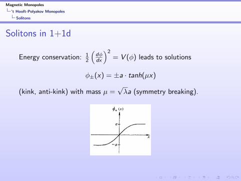
Solitons in 1+1d
Energy conservation: 12
(dφdx
)2= V (φ) leads to solutions
φ±(x) = ±a · tanh(µx)
(kink, anti-kink) with mass µ =√λa (symmetry breaking).

Magnetic Monopoles
’t Hooft-Polyakov Monopoles
Solitons
Stability and topological conservation law
Soliton mass scale ∼ symmetry breaking scale → heavy, unstable ?
φ(∞)− φ(−∞) = n · 2a with n = 0,±1
define current by jµ(x) = εµν∂νφ
→ Q =
∞∫−∞
j0(x)dx =
∞∫−∞
(∂xφ(x))dx = n(2a)
is the topologically conserved charge. Hence, n is conserved andthere should be no transitions between the states and no decay ofthe soliton to the vacuum.
Magnetic Monopoles
’t Hooft-Polyakov Monopoles
Solitons
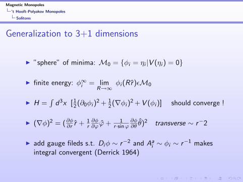
Generalization to 3+1 dimensions
I ”sphere” of minima: M0 = {φi = ηi |V (ηi ) = 0}
I finite energy: φ∞i = limR→∞
φi (Rr)εM0
I H =∫
d3x [12(∂0φi )2 + 1
2(∇φi )2 +V (φi )] should converge !
I (∇φ)2 = (∂φ∂r r + 1
r∂φ∂ϕ ϕ+ 1
r ·sin ϕ∂φ∂θ θ)
2 transverse ∼ r−2
I add gauge fileds s.t. Diφ ∼ r−2 and Aai ∼ φi ∼ r−1 makes
integral convergent (Derrick 1964)

Magnetic Monopoles
’t Hooft-Polyakov Monopoles
SO(3)
The Georgi-Glashow-SO(3) model
Consider SO(3)-model with Higgs-Triplet in adj. representation:
L =1
2(Dµφ)a(Dµφ)a − 1
4Fµν
a F aµν − V (φ)
with the potential, fields and cov. derivatives given by:
F aµν = ∂µAa
ν − ∂νAaµ − eεabcAb
µAcν
(Dµφ)a = ∂µφa − eεabcAb
µφc
V (φ) =λ
4(φ2 − a2)2
Magnetic Monopoles
’t Hooft-Polyakov Monopoles
SO(3)
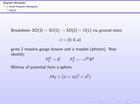
Breakdown SO(3) ∼ SU(2) → SO(2) ∼ U(1) via ground state:
φ = (0, 0, a)
gives 2 massive gauge bosons and a massles (photon). Nowidentify:
F 0i3 = E i F ij
3 = −εijkBk
Minima of potential form a sphere:
M0 = {φ = η|η2 = a2}

Magnetic Monopoles
’t Hooft-Polyakov Monopoles
’t Hooft Polyakov Soliton
t’Hooft-Polyakov Ansatz
We need Diφ ∼ r−2 and Aai ∼ φa ∼ r−1 for H to converge.
In addition we want φ∞i = limR→∞
φi = ηi = a · r
Ansatz by ’t Hooft and Polyakov (1974):
φb =rb
er2H(aer) Ai
b = −εbijr j
er2(1− K (aer)) A0
b = 0
Energy of system given by Hamiltonian:
E =4πa
e
∞Z0
dξ
ξ2
"ξ2
„dK
dξ
«2
+1
2
„ξdH
dξ− H
«2
+1
2(K2 − 1)2 + K2H2 +
λ
4e2(H2 − ξ2)2
#
with ξ = aer .
Magnetic Monopoles
’t Hooft-Polyakov Monopoles
’t Hooft Polyakov Soliton
E =4πa
e
∞Z0
dξ
ξ2
"ξ
2„
dK
dξ
«2
+1
2
„ξ
dH
dξ− H
«2
+1
2(K2 − 1)2 + K2H2 +
λ
4e2(H2 − ξ
2)2#
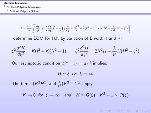
determine EOM for H,K by variation of E w.r.t H and K:
ξ2d2K
dξ2= KH2 + K (K 2 − 1) ξ2
d2H
dξ2= 2K 2H +
λ
e2H(H2 − ξ2)
Our asymptotic condition φ∞i = ηi = a · r implies:
H ∼ ξ for ξ →∞
The terms (K 2H2) and 1ξ2 (K
2 − 1)2 imply:
K → 0 for ξ →∞ and H ≤ O(ξ) K 2 − 1 ≤ O(ξ)

Magnetic Monopoles
’t Hooft-Polyakov Monopoles
’t Hooft Polyakov Soliton
The mass of this (static) solution is given by its Energy, theintegral can be solved numerically and is ≈ 1, so we have:
M ≈ 4πa
e
so the mass is set by vev of the scalar field which is also a scale forsymmetry breaking SO(3) → SO(2).
Magnetic Monopoles
’t Hooft-Polyakov Monopoles
The ’t Hooft-Polyakov-Monopole
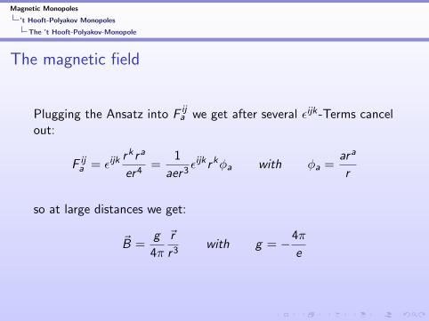
The magnetic field
Plugging the Ansatz into F ija we get after several εijk -Terms cancel
out:
F ija = εijk
rk ra
er4=
1
aer3εijk rkφa with φa =
ara
r
so at large distances we get:
~B =g
4π
~r
r3with g = −4π
e
Magnetic Monopoles
’t Hooft-Polyakov Monopoles
The ’t Hooft-Polyakov-Monopole
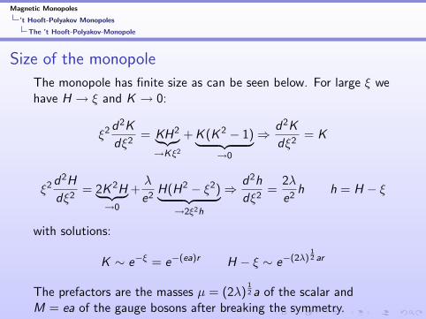
Size of the monopole
The monopole has finite size as can be seen below. For large ξ wehave H → ξ and K → 0:
ξ2d2K
dξ2= KH2︸︷︷︸→Kξ2
+K (K 2 − 1)︸ ︷︷ ︸→0
⇒ d2K
dξ2= K
ξ2d2H
dξ2= 2K 2H︸ ︷︷ ︸
→0
+λ
e2H(H2 − ξ2)︸ ︷︷ ︸
→2ξ2h
⇒ d2h
dξ2=
2λ
e2h h = H − ξ
with solutions:
K ∼ e−ξ = e−(ea)r H − ξ ∼ e−(2λ)12 ar
The prefactors are the masses µ = (2λ)12 a of the scalar and
M = ea of the gauge bosons after breaking the symmetry.

Magnetic Monopoles
’t Hooft-Polyakov Monopoles
The ’t Hooft-Polyakov-Monopole
Summary
I At large distances behaves like Dirac monopole
I finite size and smooth structure, no point charge
I classical mass of order of symmetry breaking
I no singularities like Dirac string
Related Documents