Magnetic Methods - University of Nevada, Renocrack.seismo.unr.edu/.../AppliedGPH_MagneticMethods.pdf · Magnetic Methods 3.1. INTRODUCTION 3.1 .I. General ... tity involved in magnetic

Chapter 3

Magnetic Methods

3.1. INTRODUCTION

3.1 .I. General

Magnetic and gravity methods have much in common, but magnetics is generally more complex and variations in the magnetic field are more erratic and localized. This is partly due to the difference between the dipolar magnetic field and the monopolar gravity field, partly due to the variable direction of the magnetic field, whereas the gravity field is always in the vertical direction, and partly due to the time- dependence of the magnetic field, whereas the gravity field is time-invariant (ignoring small tidal variations). Whereas a gravity map usually is dominated by regional effects, a magnetic map generally shows a multitude of local anomalies. Magnetic measurements are made more easily and cheaply than most geophysical measurements and corrections are practically unnecessary. Magnetic field variations are often diagnostic of mineral structures as well as regional structures, and the magnetic method is the most versatile of geophysical prospecting techniques. However, like all potential methods, magnetic methods lack uniqueness of interpretation.

3.1.2. History of Magnetic Methods

The study of the earth's magnetism is the oldest branch of geophysics. It has been known for more than three centuries that the Earth behaves as a large and somewhat irregular magnet. Sir William Gilbert (1540-1603) made the first scientific investigation of terrestrial magnetism. He recorded in de Magnete that knowledge of the north-seeking property of a magnetite splinter (a lodestone or leading stone) was brought to Europe from China by Marco Polo. Gilbert showed that the Earth's magnetic field was roughly equivalent to that of a permanent magnet lying in a general north-south direction near the Earth's rotational axis.

Karl Frederick Gauss made extensive studies of the Earth's magnetic field from about 1830 to 1842, and most of his conclusions are still valid. He con- cluded from mathematical analysis that the magnetic field was entirely due to a source within the Earth, rather than outside of it, and he noted a probable connection to the Earth's rotation because the axis of the dipole that accounts for most of the field is not far from the Earth's rotational axis.

The terrestrial magnetic field has been studied almost continuously since Gilbert's time, but it was not until 1843 that von Wrede first used variations in the field to locate deposits of magnetic ore. The publication, in 1879, of The Examination of Iron Ore Deposits by Magnetic Measurements by Thalkn marked the first use of the magnetic method.

Until the late 1940s, magnetic field measurements mostly were made with a magnetic balance, which measured one component of the earth's field, usually the vertical component. This limited measurements mainly to the land surface. The fluxgate magnetometer was developed during World War I1 for detecting submarines from an aircraft. After the war, the fluxgate magnetometer (and radar navigation, another war development) made aeromagnetic measurements possible. Proton-precession magnetometers, developed in the mid-l950s, are very reliable and their operation is simple and rapid. They are the most commonly used instruments today. Optical-pump al- kali-vapor magnetometers, which began to be used in 1962, are so accurate that instrumentation no longer limits the accuracy of magnetic measurements. How- ever, proton-precession and optical-pump magnetometers measure only the magnitude, not the direction, of the magnetic field. Airborne gradiometer measurements began in the late 1960s, although ground measurements were made much earlier. The gradiometer often consists of two magnetometers vertically spaced 1 to 30 m apart. The difference in readings not only gives the vertical gradient, but also, to a large extent, removes the effects of tempo-

Principles and elementary theory

ral field variations, which are often the limiting factor on accuracy.

Digital recording and processing of magnetic data removed much of the tedium involved in reducing measurements to magnetic maps. Interpretation al- gorithms now make it possible to produce computer- drawn profiles showing possible distributions of magnetization.

The history of magnetic surveying is discussed by Reford (1980) and the state of the art is discussed by Paterson and Reeves (1985).

63

3.2. PRINCIPLES AND ELEMENTARY THEORY

3.2.1. Classical versus Electromagnetic Concepts

Modem and classical magnetic theory differ in basic concepts. Classical magnetic theory is similar to electrical and gravity theory; its basic concept is that point magnetic poles are analogous to point electrical charges and point masses, with a similar inverse- square law for the forces between the poles, charges, or masses. Magnetic units in the centimeter-gram- second and electromagnetic units (cgs and emu) system are based on this concept. Systkme International (SI) units are based on the fact that a magnetic field is electrical in origin. Its basic unit is the dipole, which is created by a circular electrical current, rather than the fictitious isolated monopole of the cgs-emu system. Both emu and SI units are in current use.

The cgs-emu system begins with the concept of magnetic force F given by Coulomb's law:

where F is the force on p2, in dynes, the poles of strength p1 and p2 are r centimeters apart, p is the magnetic permeability [a property of the medium; see Eq. (3.7)], and r1 is a unit vector directed from p1 toward p2. As in the electrical case (but unlike the gravity case, in which the force is always attractive), the magnetostatic force is attractive for poles of opposite sign and repulsive for poles of like sign. The sign convention is that a positive pole is attracted toward the Earth's north pagnetic pole; the term north-seeking is also used.

The magnetizing jield H (also called magnetic jeld strength) is defined as the force on a unit pole:

Figure 3.1. Ampere's law. A current I through a length of conductor Ai creates a magnetizing field A H at a point P:

AH = ( I A / ) x r,/4m2

where A H is in amperes per meter when I is in amperes and r and AI are in meters.

units); H is measured in oersteds (equivalent to dynes per unit pole).

A magnetic dipole is envisioned as two poles of strength + p and - p separated by a distance 21. The magnetic dipole moment is defined as

m = 2&r1 ( 3 - 3 )

m is a vector in the direction of the unit vector rl 'that extends from the negative pole toward the positive pole.

A magnetic field is a consequence of the flow of an electrical current. As expressed by Amphre's law (also called the Biot-Savart law), a current I in a conductor of length A1 creates, at a point P (Fig. 3.1), a magnetizing field AH given by

AH = (I A/) x r1/4.11r2 ( 3 -4)

where H has the SI dimension amperes per meter [= 4.11 x oersted], r and A1 are in meters, I is in amperes, and AH, r,, and I A1 have the directions indicated in Figure 3.1.

A current flowing in a circular loop acts as a magnetic dipole located at the center of the loop and oriented in the direction in which a right-handed screw would advance if turned in the direction of the current. Its dipole moment is measured in ampere- meter2 (= 10" pole-cm). The orbital motions of electrons around an atomic nucleus constitute circular currents and cause atoms to have magnetic mo-

H' = F/P2 = ( P l / P + l ( 3 . 2 )

(we use a prime to indicate that H is in cgs-em

64 Magnetic methods

ments. Molecules also have spin, which gives them magnetic moments.

A magnetizable body placed in an external magnetic field becomes magnetized by induction; the magnetization is due to the reorientation of atoms

B S

and molecules so that their spins line up. The mag- Initial magnetization netization is measured by the magnetic pofarization C U N C

M (also called magnetization intensity or dipore moment per unit volume). The lineup of internal dipoles produces a field M, which, within the body, is added to the magnetizing field H. If M is constant and has the same direction throughout, a body is said to be

is ampere-meterz per meter3 1- ampere per meter (A/m)l.

For low magnetic fields, M is proportional to H and is in the direction of H. The degree to which a body is magnetized is determined by its magnetic Susceptibility k, which is defined by

H

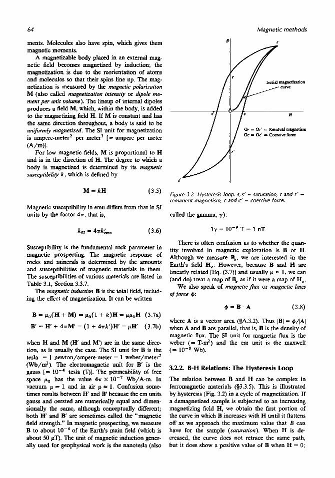
uniform& magnetized. The SI unit for magnetization Or = Or‘ = Residual magnetism of = Oc‘ = Coercive force

M = k H (3*5) Figure 3.2. Hysteresis loop. 5,s‘ = saturation, r and r’ = remanent magnetism, c and c‘ = coercive force.

Magnetic susceptibility in emu differs from that in SI units by the factor 4n, that is, called the gamma, y ) :

k, = 4nk&,,

Susceptibility is the fundamental rock parameter in magnetic prospecting. The magnetic response of rocks and minerals is determined by the amounts and susceptibilities of magnetic materials in them. The susceptibilities of various materials are listed in Table 3.1, Section 3.3.7.

The magnetic induction B is the total field, includ- ing the effect of magnetization. It can be written

B = po(H + M) = po(l + k)H = ppoH (3.7a)

B’ = H + 4nM‘ = (1 + 4~k’ )H’ = p H (3.7b)

when H and M (H’ and M’) are in the same direction, as is usually the case. The SI unit for B is the tesla = 1 newton/ampere-meter = 1 weber/meter2 (Wb/d) . The electromagnetic unit for B’ is the gauss [= ta la (T)]. The permeability of free space po has the value 4n x Wb/A-m. In vacuum p = 1 and in air p = 1. Confusion sometimes results between H’ and B’ because the em units gauss and oersted are numerically equal and dimen- sionally the same, although conceptually different; both H’ and B’ are sometimes called the “magnetic field strength.” In magnetic prospecting, we measure B to about low4 of the Earth’s main field (which is about 50 pT). The unit of magnetic induction generally used for geophysical work is the nanotesla (also

l y = T = 1 nT

There is often confusion as to whether the quan- tity involved in magnetic exploration is B or H. Although we measure Be, we are interested in the Earth’s field He. However, because B and H are linearly related [Eq. (3.7)] and usually p = 1, we can (and do) treat a map of Be as if it were a map of He.

We also speak of magneticflux or magnetic lines of force +:

+ = B * A (3.8)

where A is a vector area (5A.3.2). Thus IB/ = +/]A[ when A and B are parallel, that is, B is the density of magnetic flux. The SI unit for magnetic flu is the weber (= T-n?) and the em unit is the maxwell (= 10-8 wb).

3.2.2. B-H Relations: The Hysteresis Loop

The relation between B and H can be complex in ferromagnetic materials (53.3.5). This is illustrated by hysteresis (Fig. 3.2) in a cycle of magnetization. If a demagnetized sample is subjected to an increasing magnetizing field H, we obtain the first portion of the curve in which B increases with H until it flattens off as we approach the maximum value that B can have for the sample (saturation). When H is de- creased, the curve does not retrace the same path, but it does show a positive value of B when H = 0;

Principles and elementary theory 65

this is called residual (remanent) magnetism. When H is reversed, B finally becomes zero at some negative value of H known as the coercive force. The other half of the hysteresis loop is obtained by making H still more negative until reverse saturation is reached and then returning H to the original positive saturation value. The area inside the curve represents the energy loss per cycle per unit volume as a result of hysteresis (see Kip, 1962, pp. 235-7). Residual effects in magnetic materials will be discussed in more detail in Section 3.3.6. In some magnetic materials, B may be quite large as a result of previous magnetization having no relation to the present value of H.

3.2.3. Magnetostatic Potential for a Dipole Field -P +P

-21-

Conceptually the magnetic scalar potential A at the point P is the work done on a unit positive pole in bringing it from infinity by any path against a magnetic field F(r) [compare &. (2.4)]. (Henceforth in this chapter F, F indicate magnetic field rather than force and we assume p = 1.) When F(r) is due to a positive pole at a distance r from P,

Figure 3.3. Calculating the field of a magnetic dipole

lar component i’ & = - aA/rae; these are

{ ( rz + 12 + 2rl cos 0)3/2

i

r + IcosO F , = - p

r - IcosO - 3/2} (3.12a) A(r) = - j r - W F(r) * d r = p / r (3.9) ( r’ + I’ - 2r1 cos 0)

I sin 9

(r’ + 12 + 2rlcos0)~”

I sin 9

( r2 + 12 - 2r1 cos e)”’ } (3.12b)

F , = p However, since a magnetic pole cannot exist, we consider a magnetic dipole to get a realistic entity. Referring to Figure 3.3, we calculate A at an external point:

+

When r w I, Equation (3.10) becomes

A = (mlcos B/r2 (3.13)

1 where m is the dipole moment of magnitude m = 2[p. Equations (3.11) and (3.13) give [9A.4 and Equation (A.33)1

I/’ (r’ + I2 - 2Ircos8) = P{

F = ( m/r3)(2cos8r, + sin@) (3.14a)

where unit vectors r, and 4 are in the direction of increasing r and 9 (counterclockwise in Fig. 3.3). The resultant magnitude is We can derive the vector F by taking the gradient of

A [J3q. (A.l7)]: F = IFI = (m/r3)(1 + 3cosze)1/2 ( 3 . ~ )

F( r ) = -vA( r) (3.11) and the direction with respect to the dipole axis is

Its radial component is I;, = - aA/ar and its angu- tan a = F,/F, = (1/2) tan 9 (3.14~)

66 Magnetic methods

f z

Figure 3.4. General magnetic anomaly.

Two special cases, 0 = 0 and a/2 in Equation (3.12), are called the Gauss-A (end-on) and Gauss-B (side-on) positions. From Equations (3.12) they are given by

F, = 2 m r / ( r ~ - 12)' F, = o e = o (3.15a)

F, = o F, = m/(r2 + 1 2 ) ~ ~ ~ e = a/2 (3.15b)

If r >> 1, these simplify to

(3.15~) F, = 2m/r3

F, = m/r3

3.2.4. The General Magnetic Anomaly

A volume of magnetic material can be considered as an assortment of magnetic dipoles that results from the magnetic moments of individual atoms and dipoles. Whether they initially are aligned so that a body exhibits residual magnetism depends on its previous magnetic history. They will, however, be aligned by induction in the presence of a magnetizing field. In any case, we may regard the body as a continuous distribution of dipoles resulting in a vector dipole moment per unit volume, M, of magnitude M. The scalar potential at P [see Fig. 3.3 and Eq. (3.13)] some distance away from a dipole M ( r >> 1) is

A = M(r)cos0/rZ = -M(r) -v(l/r) (3.16)

The potential for the whole body at a point outside

the body (Fig. 3.4) is

1 A = - /M( r ) - V

V

The resultant magnetic field can be obtained by employing Equation (3.11) with Equation (3.17). This gives

1 F(ro) = v / M(r) v

V

If M is a constant vector with direction a = ei + m j + n k, then the operation

(3.19)

[Eq. (A.18)] and

A = - M - / a ( - dv ) (3.20) v Iro - rl

The magnetic field in Equation (3.20) exists in the presence of the Earth's field F,, that is, the total field F is given by

F - F, + F( ro)

where the directions of F, and F( ro) are not necessarily the same. If F( ro) is much smaller than F, or if the body has no residual magnetism, F and F, will be in approximately the same direction. Where F( ro) is an appreciable fraction (say, 25% or more) of F, and

Magnetism of the Earth 67

has a different direction, the component of F(ro) in the direction of F,, FD, becomes [Eq. (3.20)]

(3.21a)

where f, is a unit vector in the direction of F, (53.3.2a). If the magnetization is mainly induced by F,, then

a 2 dv a 2 dv

af2 vlro - rl FD(ro) = M--/ - - - kc--/- afz vlro - rl

(3.21b)

The magnetic interpretation problem is clearly more complex than the gravity problem because of the dipolar field (compare $2.2.3).

The magnetic potential A, like the gravitational potential U, satisfies Laplace’s and Poisson’s equations. Following the method used to derive Equa- tions (2.12) and (2.13), we get

v . F = -V2A = 4 ~ p p

p is the net positive pole strength per unit volume at a point. We recall that a field F produces a partial reorientation along the field direction of the previ- ously randomly oriented elementary dipoles. This causes, in effect, a separation of positive and negative poles. For example, the x component of F separates pole strengths + q and -4 by a distance { along the x axis and causes a net positive pole strength (43) cj, dz = M, 4d.z to enter the rear face in Figure A.2a. Because the pole strength leaving through the opposite face is {M, + (aM,/dx) dx} dydz, the net positive pole strength per unit volume ( p ) created at a point by the field F is - v - M. Thus,

v2A = 47rpv - M( r) (3.22)

In a nonmagnetic medium, M = 0 and

v2A = 0 (3.23)

3.2.5. Poisson‘s Relation

If we have an infinitesimal unit volume with magnetic moment M = Mal and density p, then at a distant point we have, from Equation (3.16),

A = - M * V ( l / r ) -MV(l / r ) (3.24)

From Equations (2.3a), (2.5), and (A.18), the compo-

nent of g in the direction a, is

g, = -dU/da = - v U . a, = -ypV(l/r) . a, (3.25)

Thus,

If we apply this result to an extended body, we must sum contributions for each element of volume. Provided that M and p do not change throughout the body, the potentials A and U will be those for the extended body. Therefore, Equations (3.24) to (3.26) are valid for an extended body with constant density and uniform magnetization.

In terms of fields,

where U, = dU/da. For a component of F in the direction &, this becomes

In particular, if M is vertical, the vertical component of F is

These relations are used to make pseudogravity maps from magnetic data.

3.3. MAGNETISM OF THE EARTH

3.3.1. Nature of the Geomagnetic Field

As far as exploration geophyics is concerned, the geomagnetic field of the Earth is composed of three parts: 1. The main field, which varies relatively slowly and

is of internal origin. 2. A small field (compared to the main field), which

varies rather rapidly and originates outside the Earth.

3. Spatial variations of the main field, which are usually smaller than the main field, are nearly constant in time and place, and are caused by local magnetic anomalies in the near-surface crust of the Earth. These are the targets in magnetic prospecting.

68 Magnetic methods

or positive pole; the end that dips downward in southern latitudes is the south-seeking or negative pole.

Maps showing lines of equal declination, inclination, horizontal intensity, and so on, are called iso- magnetic maps (Fig. 3.6). Isogonic, isoclinic, and isodynamic maps show, respectively, lines of equal declination D, inclination I, and equal values of F,, He, or Z,. Note that the inclination is large (that is, Z, > He) for most of the Earth's land masses, and hence corrections do not have to be made for latitude variations of F, or Z, (= 4 nT/km) except for surveys covering extensive areas. The overall magnetic field does not reflect variations in surface geol- ogy, such as mountain ranges, mid-ocean ridges or earthquake belts, so the source of the main field lies deep within the Earth. The geomagnetic field resem- bles that of a dipole whose north and south magnetic poles are located approximately at 75"N, lOl'W and 69'S,145"E. The dipole is displaced about 300 km from the Earth's center toward Indonesia and is inclined some 11.5' to the Earth's axis. However, the geomagnetic field is more complicated than the field of a simple dipole. The points where a dip needle is vertical, the dip poles, are at 75'N,lOloW and 67'S, 143'E.

The magnitudes of F, at the north and south magnetic poles are 60 and 70 pT, respectively. The minimum value, - 25 pT, occurs in southern Brazil --South Atlantic. In a few locations, F, is larger than 300 pT because of near-surface magnetic features. The line of zero inclination (magnetic equator, where Z = 0) is never more than 15" from the Earth's equator. The largest deviations are in South America and the eastern Pacific. In Africa and Asia it is slightly north of the equator.

z

Figure 3.5. Elements of the Earth's magnetic field.

3.3.2. The Main Field

(a) The Earth's magnetic field. If an unmagnetized steel needle could be hung at its center of gravity, so that it is free to orient itself in any direction, and if other magnetic fields are absent, it would assume the direction of the Earth's total magnetic field, a direction that is usually neither horizontal nor in-line with the geographic meridian. The magnitude of this field, F, , the inclination (or dip) of the needle from the horizontal, I, and the angle it makes with geographic north (the declination), D, completely define the main magnetic field.

The magnetic elements (Whitham, 1960) are illustrated in Figure 3.5. The field can also be described in terms of the vertical component, Z,, reckoned positive downward, and the horizontal component, He, which is always positive. X, and % are the components of He, which are considered positive to the north and east, respectively. These elements are related as follows:

I F,' = H,' + Z,' = X,' + r,' + Z,'

He = F,ws I Z , = F, sin I

(3.29) X , = H , c o s D T = H , s i n D

tan D = %/X, tan I = Z,/H,

I F, = F,f, = F,(cos Dcos Ii

+ s i n D c o s I j + sinIk),

As stated earlier, the end of the needle that dips downward in northern latitudes is the north-seeking

(b) Origin of the main field. Spherical harmonic analysis of the observed magnetic field shows that over 99% is due to sources inside the Earth. The present theory is that the main field is caused by convection currents of conducting material circulat- ing in the liquid outer core (which extends from depths of 2,800 to 5,000 km). The Earth's core is assumed to be a mixture of iron and nickel, both good electrical conductors. The magnetic source is thought to be a self-excited dynamo in which highly conductive fluid moves in a complex manner caused by convection. Paleomagnetic data show that the magnetic field has always been r o u a y along the Earth's spin axis, implying that the convective m e tion is coupled to the Earth's spin. Recent exploration of the magnetic fields of other planets and their satellites provide fascinating comparisons with the Earth's field.

Figure 3.6. The Earth’s magnetic field in 1975. (From Smith, 1982). (a) Declination (heavy lines) and annual rate of change in minutes/year (light lines)

Figure 3.6. (Continued) (b) geomagnetic latitude (heavy lines) and annual rate of change in minutes/year (light lines)

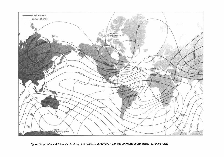
Figure 3.6. (Continued) (c) total field strength in nanotesla (heavy lines) and rate of change in nanotesla/year (light lines).

72 Magnetic methods

the Canadian Shield, for example, shows a magnetic contrast to the Western Plains). Many large, erratic variations often make magnetic maps extremely complex. The sources of local magnetic anomalies cannot be very deep, because temperatures below - 40 km should be above the Curie point, the temperature (= 550°C) at which rocks lose their magnetic properties. Thus, local anomalies must be associated with features in the upper crust.

(c) Secular variations of the main field. Four hundred years of continuous study of the Earth's field has established that it changes slowly. The inclha- tion has changed some 10" (75" to 65") and the declination about 35" (10'E to 25"W and back to loow) during this period. The source of this wander- ing is thought to be changes in convection currents in the core.

The Earth's magnetic field has also reversed direction a number of times. The times of many of the periodic field reversals have been ascertained and provide a magnetochronographic time scale.

3.3.3. The External Magnetic Field

Most of the remaining small portion of the geomagnetic field appears to be associated with electric currents in the ionized layers of the upper atmo- sphere. Time variations of this portion are much more rapid than for the main "permanent" field. Some effects are:

A cycle of 11 years duration that correlates with sunspot activity. Solar diurnal variations with a period of 24 h and a range of 30 nT that vary with latitude and season, and are probably controlled by action of the solar wind on ionospheric currents. Lunar variations with a 25 h period and an amplitude 2 nT that vary cyclically throughout the month and seem to be associated with a Moon-ionosphere interaction. Magnetic storms that are transient disturbances with amplitudes up to 1,OOO nT at most latitudes and even larger in polar regions, where they are associated with aurora. Although erratic, they often occur at 27 day intervals and correlate with sunspot activity. At the height of a magnetic storm (which may last for several days), long-range radio reception is affected and magnetic prospecting may be impractical.

These time and soace variations of the Earth's main field do not significantly affect magnetic prospecting except for the occasional magnetic storm. Diurnal variations can be corrected for by use of a base-station magnetometer. Latitude variations (= 4 nT/km) require corrections only for high-resolution, high-latitude, or large-scale surveys.

3.3.4. local Magnetic Anomalies

Local changes in the main field result from variations in the magnetic mineral content of near-surface rocks. These anomalies occasionally are large enough to double the main field. They usually do not persist over great distances; thus magnetic maps generally do not exhibit large-scale regional features (although

3.3.5. Magnetism of Rocks and Minerals

Magnetic anomalies are caused by magnetic minerals (mainly magnetite and pyrrhotite) contained in the rocks. Magnetically important minerals are surpris- ingly few in number.

Substances can be divided on the basis of their behavior when placed in an external field. A substance is diamagnetic if its field is dominated by atoms with orbital electrons oriented to oppose the external field, that is, if it exhibits negative susceptibility. Diamagnetism will prevail only if the net magnetic moment of all atoms is zero when H is zero, a situation characteristic of atoms with completely filled electron shells. The most common diamagnetic earth materials are graphite, marble, quartz, and salt. When the magnetic moment is not zero when H is zero, the susceptibility is positive and the substance is paramagnetic. The effects of diamagnetism and most paramagnetism are weak.

Certain paramagnetic elements, namely iron, cobalt, and nickel, have such strong magnetic interaction that the moments align within fairly large regions called domains. This effect is called ferromagnetism and it is - lo6 times the effects of diamagnetism and paramagnetism. Ferromagnetism decreases with increasing temperature and disap- pears entirely at the Curie temperature. Apparently ferromagnetic minerals do not exist in nature.

The domains in some materials are subdivided into subdomains that align in opposite directions so that their moments nearly cancel; although they would otherwise be considered ferromagnetic, the susceptibility is comparatively low. Such a substance is antiferromagnetic. The only common example is hematite.

In some materials, the magnetic subdomains align in opposition but their net moment is not zero, either because one set of subdomains has a stronger magnetic alignment than the other or because there are more subdomains of one type than of the other. These substances are ferrimagnetic. Examples of the first type are magnetite and titanomagnetite, oxides of iron and of iron and titanium. Pyrrhotite is a magnetic mineral of the second type. Practically all magnetic minerals are femmagnetic.

Magnetism of the Earth

3.3.6. Remanent Magnetism

In many cases, the magnetization of rocks depends mainly on the present geomagnetic field and the magnetic mineral content. Residual magnetism (called natural remanent magnetization, NRM) often contributes to the total magnetization, both in amplitude and direction. The effect is complicated because NRM depends on the magnetic history of the rock. Natural remanent magnetization may be due to several causes. The principal ones are:

1. Thermoremanent magnetization (TRM), which results when magnetic material is cooled below the Curie point in the presence of an external field (usually the Earth's field). Its direction depends on the direction of the field at the time and place where the rock cooled. Remanence acquired in this fashion is particularly stable. This is the main mechanism for the residual magnetization of igneous rocks.

2. Detrital magnetization (DRM), which occurs during the slow settling of fine-grained particles in the presence of an external field. Varied clays exhibit this type of remanence.

3. Chemical remanent magnetization (CRM), which takes place when magnetic grains increase in size or are changed from one form to another as a result of chemical action at moderate temperatures, that is, below the Curie point. This process may be significant in sedimentary and metamorphic rocks.

4. Isothermal remunent magnetization (IRM), which is the residual left following the removal of an external field (see Fig. 3.2). Lightning strikes produce IRM over very small areas.

5 . Viscous remanent magnetization (VRM), which is produced by long exposure to an external field; the buildup of remanence is a logarithmic function of time. VRM is probably more characteristic of fine-grained than coarse-grained rocks. This remanence is quite stable.

Studies of the magnetic history of the Earth (paleomagnetism) indicate that the Earth's field has varied in magnitude and has reversed its polarity a number of times (Strangway, 1970). Furthermore, it appears that the reversals took place rapidly in geologic time, because there is no evidence that the Earth existed without a magnetic field for any significant period. Model studies of a self-excited dynamo show such a rapid turnover. Many rocks have remanent magnetism that is oriented neither in the direction of, nor opposite to, the present Earth field. Such results support the plate tectonics theory. Paleomag- netism helps age-date rocks and determine past movements, such as plate rotations. Paleomagnetic

73

laboratory methods separate residual from induced magnetization, something that cannot be done in the field.

3.3.7. Magnetic Susceptibilities of Rocks and Minerals

Magnetic susceptibility is the significant variable in magnetics. It plays the same role as density does in gravity interpretation. Although instruments are available for measuring susceptibility in the field, they can only be used on outcrops or on rock samples, and such measurements do not necessarily give the bulk susceptibility of the formation.

From Figure 3.2, it is obvious that k (hence p also) is not constant for a magnetic substance; as H increases, k increases rapidly at first, reaches a maximum, and then decreases to zero. Furthermore, although magnetization curves have the same general shape, the value of H for saturation varies greatly with the type of magnetic mineral. Thus it is important in making susceptibility determinations to use a value of H about the same as that of the Earth's field.

Since the femmagnetic minerals, particularly magnetite, are the main source of local magnetic anomalies, there have been numerous attempts to establish a quantitative relation between rock susceptibility and FqO, concentration. A rough linear dependence (k ranging from to 1 SI unit as the volume percent of Fe304 increases from 0.05% to 35%) is shown in one report, but the scatter is large, and results from other areas differ.

Table 3.1 lists magnetic susceptibilities for a variety of rocks. Although there is great variation, even for a particular rock, and wide overlap between different types, sedimentary rocks have the lowest average susceptibility and basic igneous rocks have the highest. In every case, the susceptibility depends only on the amount of ferrimagnetic minerals present, mainly magnetite, sometimes titano-magnetite or pyrrhotite. The values of chalcopyrite and pyrite are typical of many sulfide minerals that are basi- cally nonmagnetic. It is possible to locate minerals of negative susceptibility, although the negative values are very small, by means of detailed magnetic surveys. It is also worth noting that many iron minerals are only slightly magnetic.

3.3.8. Magnetic Susceptibility Measurements

(a) Measurement of k . Most measurements of k involve a comparison of the sample with a standard. The simplest laboratory method is to compare the deflection produced on a tangent magnetometer by a

74 Magnetic methods

Table 3.1. Magnetic susceptibiliies of various rocks and minerals.

Susceptibility x lo3 (SI)

Type Range Average

Sedimentary Dolomite Limestones Sandstones Shales Av. 48 sedimentary

Amphibolite Schist Phyllite Gneiss Quartzite Serpentine Slate Av. 61 metamorphic

Granite Rhyolite Dolorite Augi te-syenite Olivine-diabase Diabase Porphyry Gabbro Basalts Diorite Pyroxenite Peridotite Andesite Av. acidic igneous Av. basic igneous

Minerals Graphite Quartz Rock salt Anhydrite, gypsum Calcite Coal Clays Chalcopyrite Sphalerite Cassiterite Siderite Pyrite Limonite Arsenopyrite Hematite Chromite Franklinite Pyrrhotite llmenite Magnetite

Metamorphic

igneous

0-0.9 0 -3 0-20

0.01 - 15 0-18

0.3 - 3

0.1 - 25

3-17 0-35 0-70

s

0-50 0.2 - 35

1-35 30-40

1-160 0.3 - 200

1-90 0.2 - 1 75 0.6 - 120

90- 200

0-80 0.5 - 97

-0.001 - - 0.01

1 - 4 0.05 - 5

0.5 - 35 3-110

1 -6Ooo 300 - 3500

1200 - 19200

0.1 0.3 0.4 0.6 0.9

0.7 1.4 1.5

4

6 4.2

2.5

17

25 55 60 70 70 85

125 150 160

25 a

0.1 - 0.01 - 0.01 - 0.01

0.02 0.2 0.4 0.7 0.9

1.5 2.5 3 6.5 7

430 1500 1800 6000

Field instruments for magnetic measurements

prepared sample (either a drill core or powdered rock in a tube) with that of a standard sample of magnetic material (often FeCl, powder in a test tube) when the sample is in the Gauss-A position [Eq. (3.15a)l. The susceptibility of the sample is found from the ratio of deflections:

75

d, and dsrd are the deflections for the sample and standard, respectively. The samples must be of the same size.

A similar comparison method employs an inductance bridge (Hague, 1957) having several air-core coils of different cross sections to accommodate samples of different sizes. The sample is inserted into one of the coils and the bridge balance condition is compared with the bridge balance obtained when a standard sample is in the coil. The bridge may be calibrated to give susceptibility directly, in which case the sample need not have a particular geometry (although the calibration may not be valid for samples of highly irregular shape). This type of instrument with a large diameter coil is used in field measurements on outcrop. The bridge is balanced first with the coil remote from the outcrop and then lying on it. A calibration curve obtained with a standard relates k and the change in inductance.

(b) Measurement of remanent magnetism. Mea- surement of remanent susceptibilty is considerably more complicated than that of k. One method uses an astatic magnetometer, which consists of two magnets of equal moment that are rigidly mounted parallel to each other in the same horizontal plane with opposing poles. The magnetic system is suspended by a torsion fiber. The specimen is placed in various orientations below the astatic system and the angular deflections are measured. This device, in effect, measures the magnetic field gradient, so that extraneous fields must either be eliminated or made uniform over the region of the sample. Usually the entire assembly is mounted inside a three-component coil system that cancels the Earth's field.

Another instrument for the analysis of the residual component is the spinner magnetometer. The rock sample is rotated at high speed near a small pickup coil and its magnetic moment generates alter- nating current (ac) in the coil. The phase and intensity of the coil signal are compared with a reference signal generated by the rotating system. The total moment of the sample is obtained by rotating it about different axes.

Cryogenic instruments for determining two- axes remanent magnetism have been developed (Zimmerman and Campbell, 1975; Weinstock and

Overton, 1981). They achieve great sensitivity because of the high magnetic moments and low noise obtainable at superconducting temperatures.

3.4. FIELD INSTRUMENTS FOR MAGNETIC MEASUREMENTS

3.4.1. General

Typical sensitivity required in ground magnetic instruments is between 1 and 10 nT in a total field rarely larger than 50,000 nT. Recent airborne applications, however, have led to the development of magnetometers with sensitivity of 0.001 nT. Some magnetometers measure the absolute field, although this is not a particular advantage in magnetic surveying.

The earliest devices used for magnetic exploration were modifications of the mariner's compass, such as the Swedish mining compass, which measured dip I and declination D. Instruments (such as magnetic variometers, which are essentially dip needles of high sensitivity) were developed to measure Z, and He, but they are seldom used now. Only the modem instruments, the fluxgate, proton-precession, and optical-pump (usually rubidium-vapor) magnetometers, will be discussed. The latter two measure the absolute total field, and the fluxgate instrument also generally measures the total field.

3.4.2. Fluxgate Magnetometer

This device was originally developed during World War I1 as a submarine detector. Several designs have been used for recording diurnal variations in the Earth's field, for airborne geomagnetics, and as portable ground magnetometers.

The fluxgate detector consists essentially of a core of magnetic material, such as mu-metal, permalloy, or ferrite, that has a very high permeability at low magnetic fields. In the most common design, two cores are each wound with primary and secondary coils, the two assemblies being as nearly as possible identical and mounted parallel so that the windings are in opposition. The two primary windings are connected in series and energized by a low frequency (50 to 1,OOO Hz) current produced by a constant current source. The maximum current is sufficient to magnetize the cores to saturation, in opposite polarity, twice each cycle. The secondary coils, which consist of many turns of fine wire, are connected to a diferential ampli$er, whose output is proportional to the difference between two input signals.

The effect of saturation in the fluxgate elements is illustrated in Figure 3.7. In the absence of an external magnetic field, the saturation of the cores is

76 Magnetic methods

Primary a in the 2

Figure 3.7. Principle of the fluxgate magnetometer. Note that He = &, etc. (From Whitham, 1960.) (a) Magnetization of the cores. (b) Flux in the two cores for F, = 0. (c) Flux in the two cores for F, # 0. (d) 6 + F, for F, # 0. (e) Output voltage for F, # 0.

symmetrical and of opposite sign near the peak of each half-cycle so that the outputs from the two secondary windings cancel. The presence of an external field component parallel to the cores causes saturation to occur earlier for one half-cycle than the other, producing an unbalance. The difference between output voltages from the secondary windings is a series of voltage pulses which are fed into the amplifier, as shown in Figure 3.7d. The pulse height is proportional to the amplitude of the biasing field of the Earth. Obviously any component can be measured by suitable orientation of the cores.

The original problem with this type of magnetometer- a lack of sensitivity in the core- has been solved by the development and use of materials having sufficient initial permeability to saturate in small fields. Clearly the hysteresis loop should be as thin as possible. There remains a relatively high noise level, caused by hysteresis effects in the core. The fluxgate elements should be long and thin to reduce eddy currents. Improvements introduced to increase the signal-tcmoise ratio include the following:

1. By deliberately unbalancing the two elements, voltage spikes are present with or without an ambient field. The presence of the Earth's field increases the voltage of one polarity more than the other and this difference is amplified.

2. Because the odd harmonics are canceled fairly Figure 3.8. Portable fluxgate magnetometer.

Field instruments for rnagnetic.measurements 77

Earth's magnetic field Magnetic

on proton-

Spin ,momentum

Gyration

. /"" Moment

Gravitational

Earth's & gravity field

Figure 3.9. Proton precession and spinning-top analogy.

well in a reasonably matched set of cores, the even harmonics (generally only the second is significant) are amplified to appear as positive or negative signals, depending on the polarity of the Earth's field.

3. Most of the ambient field is canceled and variations in the remainder are detected with an extra secondary winding.

4. Negative feedback of the amplifier outputs is used to reduce the effect of the Earth's field.

5 . By tuning the output of the secondary windings with a capacitance, the second harmonic is greatly increased; a phase-sensitive detector, rather than the difference amplifier, may be used with this arrangement.

There are several fundamental sources of error in the fluxgate instrument. These include inherent unbalance in the two cores, thermal and shock noise in cores, drift in biasing circuits, and temperature sensitivity (1 nT/"C or less). These disadvantages are minor, however, compared to the obvious advantages - direct readout, no azimuth orientation, rather coarse leveling requirements, light weight (2 to 3 kg), small size, and reasonable sensitivity. Another attractive feature is that any component of the magnetic field may be measured. No elaborate tripod is required and readings may be made very quickly, generally in about 15 s. A portable fluxgate instrument is shown in Figure 3.8.

3.4.3. Proton-Precession Magnetometer

This instrument grew out of the discovery, around 1945, of nuclear magnetic resonance. Some nuclei

have a net magnetic moment that, coupled with their spin, causes them to precess about an axial magnetic field.

The proton-precession magnetometer depends on the measurement of the free-precession frequency of protons (hydrogen nuclei) that have been polarized in a direction approximately normal to the direction of the Earth's field. When the polarizing field is suddenly removed, the protons precess about the Earth's field like a spinning top; the Earth's field supplies the precessing force corresponding to that of gravity in the case of a top. The analogy is illustrated in Figure 3.9. The protons precess at an angular velocity w, known as the Larmor precession frequency, which is proportional to the magnetic field F, so that

o = y p F (3.30a)

The constant y, is the gyromagnetic ratio of the proton, the ratio of its magnetic moment to its spin angular momentum. The value of y, is known to an accuracy of 0.001%. Since precise frequency measurements are relatively easy, the magnetic field can be determined to the same accuracy. The proton, which is a moving charge, induces, in a coil sur- rounding the sample, a voltage that varies at the precession frequency v. Thus we can determine the magnetic field from

F = 21rv/y, (3.30b)

where the factor 277/yp = 23.487 Only the total field may be measured.

0.002 nT/Hz.

78

Power rupply to nopnet icol ly po lar i ze sample

Magnetic methods

Counter to open pate 1 af te r about 100 cycles -, Gote have 'passed

Oscillotion of known frequency

Figure 3.10. Proton-precession magnetometer. (From Sheriff, 1984.)

The essential components of this magnetometer include a source of protons, a polarizing magnetic field considerably stronger than that of the Earth and directed roughly normal to it (the direction of this field can be off by 45"), a pickup coil coupled tightly to the source, an amplifier to boost the minute voltage induced in the pickup coil, and a frequency- measuring device. The latter operates in the audio range because, from Equation (3.30b), v = 2130 Hz for F, = 50,000 nT. It must also be capable of indi- cating frequency differences of about 0.4 Hz for an instrument sensitivity of 10 nT.

The proton source is usually a small bottle of water (the nuclear moment of oxygen is zero) or some organic fluid rich in hydrogen, such as alcohol. The polarizing field of 5 to 10 mT is obtained by passing direct current through a solenoid wound around the bottle, which is oriented roughly east-west for the measurement. When the solenoid current is abruptly cut off, the proton precession about the Earth's field is detected by a second coil as a transient voltage building up and decaying over an interval of - 3 s, modulated by the precession frequency. In some models the same coil is used for both polarization and detection. The modulation signal is amplified to a suitable level and the frequency measured. A schematic diagram is shown in Figure 3.10.

The measurement of frequency may be carried out by actually counting precession cycles in an exact time interval, or by comparing them with a very stable frequency generator. In one ground model, the precession signal is mixed with a signal from a local oscillator of high precision to produce low-frequency beats (= 100 Hz) that drive a vibrat- ing reed frequency meter. Regardless of the method used, the frequency must be measured to an accuracy of 0.001% to realize the capabilities of the method. Although this is not particularly difficult in

a fixed installation, it posses some problems in small portable equipment.

The proton-precession magnetometer's sensitivity (= 1 nT) is high, and it is essentially free from drift. The fact that it requires no orientation or leveling makes it attractive for marine and airborne operations. It has essentially no mechanical parts, although the electronic components are relatively complex. The main disadvantage is that only the total field can be measured. It also cannot record continuously because it requires a second or more between readings. In an aircraft traveling at 300 km/hr, the distance interval is about 100 m. Proton-precession magnetometers are now the dominant instrument for both ground and airborne applications.

3.4.4. Optically Pumped Magnetometer

A variety of scientific instruments and techniques has been developed using the energy in transferring atomic electrons from one energy level to another. For example, by irradiating a gas with light or radio-frequency waves of the proper frequency, electrons may be raised to a higher energy level. If they can be accumulated in such a state and then suddenly returned to a lower level, they release some of their energy in the process. This energy may be used for amplification (masers) or to get an intense light beam, such as that produced by a laser.

The optically pumped magnetometer is another application. The principle of operation may be un- derstood from an examination of Figure 3.11a, which shows three possible energy levels, A,, A,, and B for a hypothetical atom. Under normal conditions of pressure and temperature, the atoms occupy ground state levels A, and A,. The energy difference between A, and A, is very small [= lo-' electron volts (ev)], representing a fine structure due to atomic electron spins that normally are not all aligned in the

Field instruments for magnetic measurements 79

(4 (b)

Figure 3.11. Optical pumping. (a) Energy level transitions. (b) Effect of pumping on light transmission.

same direction. Even thermal energies (= lo-' eV) are much larger than this, so that the atoms are as likely to be in level A, as in A , .

Level B represents a much higher energy and the transitions from A, or A , to B correspond to in- frared or visible spectral lines. If we irradiate a sample with a beam from which spectral line A,B has been removed, atoms in level A, can absorb energy and rise to B, but atoms in A , will not be excited. When the excited atoms fall back to ground state, they may return to either level, but if they fall to A,, they will be removed by photon excitation to B again. The result is an accumulation of atoms in level A, .

The technique of overpopulating one energy level in this fashion is known as optical pumping. As the atoms are moved from level A , to A , by this selec- tive process, less energy will be absorbed and the sample becomes increasingly transparent to the irradiating beam. When all atoms are in the A , state, a photosensitive detector will register a maximum current, as shown in Figure 3.11b. If now we apply an RF signal, having energy corresponding to the transition between A , and A , , the pumping effect is nullified and the transparency drops to a minimum again. The proper frequency for this signal is given by v = E / h , where E is the energy difference between A , and A , and h is Planck's constant [6.62 X 10- 34 joule-seconds].

To make this device into a magnetometer, it is necessary to select atoms that have magnetic energy sublevels that are suitably spaced to give a measure of the weak magnetic field of the Earth. Elements that have been used for this purpose include cesium, rubidium, sodium, and helium. The first three each have a single electron in the outer shell whose spin axis lies either parallel or antiparallel to an external magnetic field. These two orientations correspond to

the energy levels A , and A , (actually the sublevels are more complicated than this, but the simplifica- tion illustrates the pumping action adequately), and there is a difference of one quantum of angular momentum between the parallel and antiparallel states. The irradiating beam is circularly polarized so that the photons in the light beam have a single spin axis. Atoms in sublevel A , then can be pumped to B, gaining one quantum by absorption, whereas those in A , already have the same momentum as B and cannot make the transition.

Figure 3.12 is a schematic diagram of the rubidium-vapor magnetometer. Light from the R.b lamp is circularly polarized to illuminate the Rb vapor cell, after which it is refocused on a photocell. The axis of this beam is inclined approximately 45" to the Earth's field, which causes the electrons to precess about the axis of the field at the Larmor frequency. At one point in the precession cycle the atoms will be most nearly parallel to the light-beam direction and one- half cycle later they will be more antiparallel. In the first position, more light is transmitted through the cell than in the second. Thus the precession frequency produces a variable light intensity that flick- ers at the Larmor frequency. If the photocell signal is amplified and fed back to a coil wound on the cell, the coil-amplifier system becomes an oscillator whose frequency v is given by

F = 2 n v / y e (3.31)

where ye is the gyromagnetic ratio of the electron. For Rb, the value of ye/27r is approximately 4.67

Hz/nT whereas the corresponding frequency for F, = 50,000 nT is 233 kHz. Because ye for the electron is known to a precision of about 1 part in lo7 and because of the relatively high frequencies involved, it

80 Magnetic methods

r I I I I I I I I I I I

1 I I I I I I I I I I I I

I L _ _ _ _ _ _ _ _ _ _ _ _ _ _ _ _ _ _ _ _ _ _ _ _ _ _ _ _ 1 L - - - - A

Figure 3.72. Rubidium-vapor magnetometer (schematic).

is not difficult to measure magnetic field variations as small as 0.01 nT with a magnetometer of this type.

3.4.5. Cradiometers

The sensitivity of the optically pumped magnetometer is considerably greater than normally required in prospecting. Since 1965, optically pumped rubidium- and cesium-vapor magnetometers have been increasingly employed in airborne gradiometers. Two detectors, vertically separated by about 35 m, measure dF/dz, the total-field vertical gradient. The sensitivity is reduced by pitch and yaw of the two birds. Major improvements by the Geological Survey of Canada involve reducing the vertical separation to 1 to 2 m and using a more rigid connection between the sensors. Gradient measurements are also made in ground surveys. The two sensors on a staff in the Scintrex MP-3 proton-magnetometer system, for example, measure the gradient to f O . l nT/m. Gra- diometer surveys are discussed further in Section 3.5.5.

3.4.6. Instrument Recording

Originally the magnetometer output in airborne in- stallations was displayed by pen recorder. To achieve both high sensitivity and wide range, the graph would be “paged back” (the reference value changed) frequently to prevent the pen from running off the paper. Today recording is done digitally, but generally an analog display is also made during a survey. Some portable instruments for ground work also digitally record magnetometer readings, station coor- dinates, diurnal corrections, geological and terrain data.

3.4.7. Calibration of Magnetometers

Magnetometers may be calibrated by placing them in a suitably oriented variable magnetic field of known value. The most dependable calibration

method employs a Helmholtz coil large enough to surround the instrument. This is a pair of identical coils of N turns and radii a coaxially spaced a distance apart equal to the radius. The resulting magnetic field, for a current I flowing through the coils connected in series-aiding, is directed along the axis and is uniform within about 6% over a cylinder of diameter a and length 3a/4, concentric with the coils. This field is given by

H = 9.ONI/a ( 3.32a)

where I is in microamperes, H in nanoteslas, and a in meters. Because H varies directly with the current, this can be written

AH = 9 .ONAI /a (3.32b)

3.5. FIELD OPERATIONS

3.5.1. General

Magnetic exploration is carried out on land, at sea, and in the air. For areas of appreciable extent, surveys usually are done with the airborne magnetometer.

In oil exploration, airborne magnetics (along with surface gravity) is done as a preliminary to seismic work to establish approximate depth, topography, and character of the basement rocks. Since the susceptibilities of sedimentary rocks are relatively small, the main response is due to igneous rocks below (and sometimes within) the sediments.

Within the last few years it has become possible to extract from aeromagnetic data weak anomalies originating in sedimentary rocks, such as result from the faulting of sandstones. This results from (a) the improved sensitivity of magnetometers, (b) more precise determination of location with Doppler radar (5B.9, (c) corrections for diurnal and other temporal

Field operations 87

field variations, and (d) computer-analysis techniques to remove noise effects.

Airborne reconnaissance for minerals frequently combines magnetics with airborne EM. In most cases of followup, detailed ground magnetic surveys are carried out. The method is usually indirect, that is, the primary interest is in geological mapping rather than the mineral concentration per se. Frequently the association of characteristic magnetic anomalies with base-metal sulfides, gold, asbestos, and so on, has been used as a marker in mineral exploration. There is also, of course, an application for magnetics in the direct search for certain iron and titanium ores.

3.5.2. Airborne Magnetic Surveys

(a) General. In Canada and some other countries, government agencies have surveyed much of the country and aeromagnetic maps on a scale of 1 mile to the inch are available at a nominal sum. Large areas in all parts of the world have also been surveyed in the course of oil and mineral exploration.

The sensitivity of airborne magnetometers is generally greater than those used in ground exploration- about 0.01 nT compared with 10 to 20 nT. Because of the initial large cost of the aircraft and availability of space, it is practical to use more sophisticated equipment than could be handled in portable instruments; their greater sensitivity is use- ful in making measurements several hundred meters above the ground surface, whereas the same sensitivity is usually unnecessary (and may even be undesir- able) in ground surveys.

(b) Instrument mounting. Aside from stabilization, there are certain problems in mounting the sensitive magnetic detector in an airplane, because the latter has a complicated magnetic field of its own. One obvious way to eliminate these effects is to tow the sensing element some distance behind the aircraft. This was the original mounting arrangement and is still used. The detector is housed in a stream- lined cylindrical container, known as a bird, connected by a cable 30 to 150 m long. Thus the bird may be 75 m nearer the ground than the aircraft. A photograph of a bird mounting is shown in Figure 3.13a.

An alternative scheme is to mount the detector on a wing tip or slightly behind the tail. The stray magnetic effects of the plane are minimized by permanent magnets and soft iron or permalloy shielding strips, by currents in compensating coils, and by metallic sheets for electric shielding of the eddy currents. The shielding is a cut-and-try process, since the magnetic effects vary with the aircraft and

mounting location. Figure 3.13b shows an installation with the magnetometer head in the tail.

(c) Stabilization. Since proton-precession and optically pumped magnetometers measure total field, the problem of stable orientation of the sensing element is minor. Although the polarizing field in the proton-precession instrument must not be parallel to the total-field direction, practically any other orientation will do because the signal amplitude becomes inadequate only within a cone of about 5".

Stabilization of the fluxgate magnetometer is more difficult, because the sensing element must be maintained accurately in the F axis. This is accomplished with two additional fluxgate detectors that are oriented orthogonally with the first; that is, the three elements form a three-dimensional orthogonal coor- dinate system. The set is mounted on a small plat- form that rotates freely in all directions. When the sensing fluxgate is accurately aligned along the total-field axis, there is zero signal in the other two. Any tilt away from this axis produces a signal in the control elements that drive servomotors to restore the system to the proper orientation.

(d) Flight pattern. Aeromagnetic surveys almost always consist of parallel lines (Fig. 3.13~) spaced anywhere from 100 m to several kilometers apart. The heading generally is normal to the main geologic trend in the area and altitude usually is maintained at fixed elevations, the height being continuously recorded by radio or barometric altimeters. It is customary to record changes in the Earth's field with time (due to diurnal or more sudden variations) with a recording magnetometer on the ground. A further check generally is obtained by flying several cross lines, which verify readings at line intersections.

A drape survey, which approximates constant clearance over rough topography, is generally flown with a helicopter. It is often assumed that drape surveys minimize magnetic terrain effects, but Grauch and Campbell (1984) dispute this. Using a uniformly magnetized model of a mountain-valley system, four profiles (one level, the others at different ground clearance) all showed terrain effects. However, Grauch and Campbell recommend drape surveys over level-flight surveys because of greater sensitivity to small targets, particularly in valleys. The disadvantages of draped surveys are higher cost, operational problems, and less sophisticated interpretation techniques.

(e) Effect of variations in flight path. Altitude differences between flight lines may cause herring- bone patterns in the magnetic data. Bhattacharyya (1970) studied errors arising from flight deviations

Shoran Electronics, antenna

recorders \ / Doppler indicator 1

/ 1

antenna camera Radio altimeter Flight path

Compensating plate

/ I Compensating Magnetometer

coils head I

Doppler antenna ( b )

- Control lines ry? Total field contours --- Flight lines

( c )

Figure 3.13. Airborne magnetics. (a) Magnetometer in a bird. (b) Magnetometer in a tail mounting. (c) Flight pattern and magnetic map.

Field operations

over an idealized dike (prism) target. Altitude and heading changes produced field measurement changes that would alter interpretations based on anomaly shape measurements, such as those of slope. Such deviations are especially significant with high-resolution data.

83

(f) Aircraft location. The simplest method of locat- ing the aircraft at all times, with respect to ground location, is for the pilot to control the flight path by using aerial photographs, while a camera takes photos on strip film to determine locations later. The photos and magnetic data are simultaneously tagged at intervals. Over featureless terrain, radio navigation (see 3B.6) gives aircraft position with respect to two or more ground stations, or Doppler radar (5B.5) determines the precise flight path. Doppler radar increasingly is employed where high accuracy is required.

(g) Corrections to magnetic data. Magnetic data are corrected for drift, elevation, and line location differences at line intersections in a least-squares manner to force ties. Instrument drift is generally not a major problem, especially with proton and optically pumped magnetometers whose measurements are absolute values.

The value of the main magnetic field of the Earth is often subtracted from measurement values. The Earth's field is usually taken to be that of the Znter- national Geomagnetic Reference Field (IGRF) model.

A stationary base magnetometer is often used to determine slowly varying diurnal effects. Horizontal gradiometer arrangements help in eliminating rapid temporal variations; the gradient measurements do not involve diurnal effects. Usually no attempt is made to correct for the large effects of magnetic storms.

(h) Advantages and disadvantages of airborne magnetics. Airborne surveying is extremely attractive for reconnaissance because of low cost per kilo- meter (see Table 1.2) and high speed. The speed not only reduces the cost, but also decreases the effects of time variations of the magnetic field. Erratic near-surface features, frequently a nuisance in ground work, are considerably reduced. The flight elevation may be chosen to favor structures of certain size and depth. Operational problems associated with irregular terrain, sometimes a source of difficulty in ground magnetics, are minimized. The data are smoother, which may make interpretation easier. Finally, aeromagnetics can be used over water and in regions inaccessible for ground work.

The disadvantages in airborne magnetics apply mainly to mineral exploration. The cost for survey-

ing small areas may be prohibitive. The attenuation of near-surface features, apt to be the survey objec- tive, become limitations in mineral search.

3.5.3. Shipborne Magnetic Surveys

Both the fluxgate and proton-precession magnetometers have been used in marine operations. There are no major problems in ship installation. The sensing element is towed some distance (150 to 300 m) astern (to reduce magnetic effects of the vessel) in a water- tight housing called a Jish, which usually rides about 15 m below the surface. Stabilization is similar to that employed in the airborne bird. Use of a ship rather than an aircraft provides no advantage and incurs considerable cost increase unless the survey is carried out in conjunction with other surveys, such as gravity or seismic. The main application has been in large-scale oceanographic surveying related to earth physics and petroleum search. Much of the evidence supporting plate tectonics has come from marine magnetics.

3.5.4. Ground Magnetic Surveys

(a) General. Magnetic surveying on the ground now almost exclusively uses the portable proton-precession magnetometer. The main application is in detailed surveys for minerals, but ground magnetics are also employed in the followup of geochemical reconnaissance in base-metal search. Station spacing is usually 15 to 60 m; occasionally it is as small as 1 m. Most ground surveys now measure the total field, but vertical-component fluxgate instruments are also used. Sometimes gradiometer measurements (33.5.5) are made.

(b) Corrections. In precise work, either repeat readings should be made every few hours at a previ- ously occupied station or a base-station recording magnetometer should be employed. This provides corrections for diurnal and erratic variations of the magnetic field. However, such precautions are unnecessary in most mineral prospecting because anomalies are large (> 500 nT).

Since most ground magnetometers have a sensitivity of about 1 nT, stations should not be located near any sizeable objects containing iron, such as railroad tracks, wire fences, drill-hole casings, or culverts. The instrument operator should also not wear iron articles, such as belt buckles, compasses, knives, iron rings, and even steel spectacle frames.

Apart from diurnal effects, the reductions required for magnetic data are insignificant. The vertical gradient varies from approximately 0.03 nT/m at the poles to 0.01 nT/m at the magnetic equator. The

84 Magnetic methods

latitude variation is rarely > 6 nT/km. Thus elevation and latitude corrections are generally unnecessary.

The influence of topography on ground magnetics, on the other hand, can be very important. This is apparent when taking measurements in stream gorges, for example, where the rock walls above the station frequently produce abnormal magnetic lows. Terrain anomalies as large as 700 nT occur at steep (45') slopes of only 10 m extent in formations containing 2% magnetite (k = 0.025 SI unit) (Gupta and Fitzpatrick, 1971). In such cases, a terrain correction is required, but it cannot be applied merely as a function of topography alone because there are situ- ations (for example, sedimentary formations of very low susceptibility) in which no terrain distortion is observed.

A terrain smoothing correction may be carried out by reducing measurements from an irregular surface z = h ( x , y ) to a horizontal plane, say z = 0, above it. This can be done approximately by using a Taylor series (5A.5) with two terms:

cent. For the vertical contact, half the separation between maximum and minimum values equals the depth. Gradiometer measurements are valuable in field continuation calculations (53.7.5).

Ground gradiometer measurements (Hood and McClure, 1965) have recently been carried out for gold deposits in eastern Canada in an area where the overburden is only a few meters thick. The host quartz was located because of its slightly negative susceptibility using a vertical separation of 2 m and a station spacing of = 1 m. Gradiometer surveys have also been used in the search for archeological sites and artifacts, mapping buried stone structures, forges, kilns, and so forth (Clark, 1986; Wynn, 1986).

Vertical gradient aeromagnetic surveys (Hood, 1965) are often carried out at 150 to 300 m altitude. Detailed coverage with 100 to 200 m line spacing is occasionally obtained at 30 m ground clearance.

Two magnetometers horizontally displaced from each other are also used, especially with marine measurements where they may be separated by 100 to 200 m. This arrangement permits the elimination of rapid temporal variations so that small spatial anomalies can be interpreted with higher confidence.

3.5.5. Gradiometer Surveys

The gradient of F is usually calculated from the

3.6. MAGNETIC EFFECTS OF SIMPLE SHAPES

magnetic contour map with the aid of templates. There is, however, considerable merit in measuring the vertical gradient directly in the field. It is merely necessary to record two readings, one above the other. With instrument sensitivity of 1 nT, an elevation difference of = 1 m suffices. Then the vertical gradient is given by

where Fl and F, are readings at the higher and lower elevations, and A z is the separation distance.

Discrimination between neighboring anomalies is enhanced in the gradient measurements. For example, the anomalies for two isolated poles at depth h separated by a horizontal distance h yield separate peaks on a a F / a z profile but they have to be separated by 1.4 h to yield separate anomalies on an F profile. The effect of diurnal variations is also minimized, which is especially beneficial in high magnetic latitudes. For most of the simple shapes discussed in Section 3.6 (especially for the isolated pole, finite-length dipole, and vertical contact of great depth extent), better depth estimates can be made from the first vertical-derivative profiles than from either the Z or F profiles. For features of the first two types, the width of the profile at ( a Z / a z ) , , / 2 equals the depth within a few per-

3.6.1. General

Because ground surveys (until about 1968) measured the vertical-field component, whereas airborne surveys measured the total field, both vertical-component and total-field responses will be developed. Depth determinations are most important and lateral extent less so, whereas dip estimates are the least important and quite difficult. In this regard, aeromagnetic and electromagnetic interpretation are similar. In petroleum exploration the depth to basement is the prime concern, whereas in mineral exploration more detail is desirable. The potentialities of high resolution and vertical-gradient aeromagnetics are only now being exploited to a limited extent.

As in gravity and electromagnetics, anomalies are often matched with models. The magnetic problem is more difficult because of the dipole character of the magnetic field and the possibility of remanence. Very simple geometrical models are usually employed: isolated pole, dipole, lines of poles and dipoles, thin plate, dike (prism), and vertical contact. Because the shape of magnetic anomalies relates to the magnetic field, directions in the following sections are with respect to magnetic north (the x direction), magnetic east, and so forth, the z axis is positive downward, and we assume that locations are in the northern hemisphere. We use I for the field inclination, .$ for

Magnetic effects of simple shapes 85

0 Surface 8

-P

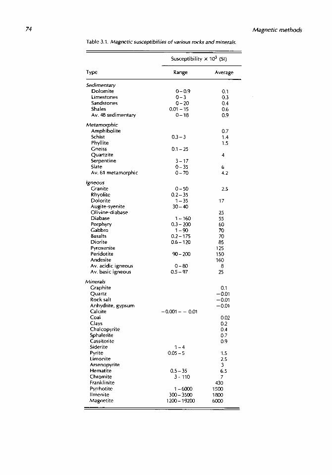
Figure 3.14. Magnetic effects of an isolated pole. (a) F, Z, and H profiles for I = 45”

the dip of bodies and /? for the strike angle relative to magnetic north (x axis). Note that depths are measured with respect to the measurement elevation (the aircraft elevation for aeromagnetic measurements).

3.6.2. The Isolated Pole (Monopole)

Although an isolated pole is a fiction, in practice it may be used to represent a steeply dipping dipole whose lower pole is so far away that it has a negltgi- ble effect. The induced magnetization in a long, slender, near-vertical body tends to be along the axis of the body except near the magnetic equator. If the length of the body is large, we have, in effect, a single negative pole - p located at (0, 0, z,,).

From Equation (3.2) or Equations (3.9) and (3.11), we get for the field at P( x, y , 0),

Fp = ( - p / r 2 ) r l = ( p / r ’ ) ( -xi - y j + zpk)

where r1 is a unit vector from P( x, y, 0) toward the pole - p . The vertical anomaly is

Usually the field of the pole, Fp, is much smaller than the field of the Earth, F,, and the total field

anomaly is approximately the component of Fp in the F, direction. Using Equation (3.29),

F Fp f1 = ( p / r ’ ) ( --xCos I + z,, sin I) (3.34b)

[Note that the total field anomaly F, which is only a component of Fp, may be smaller than Z, and that in general F # (2’ + Hz)1/2.]

Profiles are shown in Figure 3.14a for I = 45’; Z,, is located directly over the pole. The H profile is perfectly asymmetric and its positive half inter- sects the Z profile nearly at Zm,/3. The horizontal distance between positive and negative peaks of H is approximately 3zP/2. This profile is independent of the traverse direction only if the effect of the pole is much larger than the horizontal component of the Earth’s field.

A set of total-field profiles for various values of I is shown in Figure 3.14~. F,, occurs south of the monopole and F- north of it. F is zero north of the pole at x = z tan I. The curves would be re- flected in the vertical axis in southern latitudes. A total-field profile on a magnetic meridian becomes progressively more asymmetric as the inclination decreases (that is, as we move toward the magnetic equator). At the same time, the maximum decreases and the minimum increases and both are displaced progressively southward. The statement also applies

86

mag. N

HR (direction and relative magnitude:

Magnetic methods

Location of ’ isolated pole

Figure 3.14. (Continued) (b) Contours of lHRl = IH + H,I for H,, = He = 0.38. (c) F profiles for various inclinations. (After Smellie, 1967.)

Next Page

Magnetic Methods - University of Nevada, Renocrack.seismo.unr.edu/.../AppliedGPH_MagneticMethods.pdf · Magnetic Methods 3.1. INTRODUCTION 3.1 .I. General ... tity involved in magnetic

Documents