Magnetic field structures of galaxies derived from analysis of Faraday rotation measures, and perspectives for the SKA

arX

iv:0

711.

1267

v3 [

astr

o-ph

] 2

1 Ja

n 20

08Astronomy & Astrophysics manuscript no. 8678 c© ESO 2008February 2, 2008

Magnetic field structures of galaxies derived from analysis of

Faraday rotation measures, and perspectives for the SKA

Rodion Stepanov1, Tigran G. Arshakian2,⋆, Rainer Beck2, Peter Frick1, and Marita Krause2

1 Institute of Continuous Media Mechanics, Korolyov str. 1, 614061 Perm, Russia2 Max-Planck-Institut fur Radioastronomie, Auf dem Hugel 69, 53121 Bonn, Germany

Received / Accepted

ABSTRACT

Context. The forthcoming new-generation radio telescope SKA (Square Kilometre Array) and its precursors will providea rapidly growing number of polarized radio sources.Aims. Our analysis looks at what can be learned from these sources concerning the structure and evolution of magneticfields of external galaxies.Methods. Recognition of magnetic structures is possible from Faraday rotation measures (RM) towards backgroundsources behind galaxies or a continuous RM map obtained from the diffuse polarized emission from the galaxy itself. Weconstructed models for the ionized gas and magnetic field patterns of different azimuthal symmetries (axisymmetric,bisymmetric and quadrisymmetric spirals, and superpositions) plus a halo magnetic field. RM fluctuations with aKolmogorov spectrum due to turbulent fields and/or fluctuations in ionized gas density are superimposed. Assumingextrapolated number density counts of polarized sources, we generated a sample of RM values within the solid angleof the galaxy. Applying various templates, we derived the minimum number of background sources and the minimumquality of the observations. For a large number of sources, reconstruction of the field structure without precognitionbecomes possible.Results. Any large-scale regular component of the magnetic field can be clearly recognized from RM data with the helpof the χ2 criterium. Under favorite conditions, a few dozen polarized sources are enough for a reliable result. A halofield with a vertical component does not affect the results of recognition. The required source number increases forsmall inclinations of the galaxy’s disk and for larger RM turbulence. A flat number density distribution of the sourcescan be overcome by more sensitive observations. Application of the recognition method to the available RM data inthe region around M 31 indicates that there are significant RM contributions intrinsic to the background sources ordue to the foreground of the Milky Way. A reliable reconstruction of the field structure needs at least 20 RM valueson a cut along the projected minor axis.Conclusions. Recognition or reconstruction of regular field structures from the RM data of polarized background sourcesis a powerful tool for future radio telescopes. Measuring RM at frequencies around 1 GHz with the SKA, simple fieldstructures can be recognized in galaxies up to about 100 Mpc distance and will allow to test dynamo against primordialor other models of field origin. The low-frequency SKA array and low-frequency precursor telescopes like LOFAR mayalso have good RM sensitivity if background sources are still significantly polarized at low frequencies.

Key words. Methods: statistical – techniques: polarimetric – galaxies: magnetic fields – galaxies: spiral – galaxies:individual: M 31 – radio continuum: galaxies

1. Introduction

Magnetic fields play an important role for the structure andevolution of galaxies. Radio synchrotron emission providesthe best tools for measuring the strength and structure ofgalactic magnetic fields (Beck et al. 1996). However, thesensitivity of present-day radio observations only allows de-tailed studies for a couple of nearby galaxies (Beck 2005).

Rotation measures (RM) towards polarized backgroundsources located behind spiral galaxies can trace regularmagnetic fields in these galaxies out to large distances, evenwhere the synchrotron emission of the galaxy itself is tooweak to be detected (Han et al. 1998; Gaensler et al. 2005).

Send offprint requests to: R.Stepanov, e-mail: [email protected];R.Beck, e-mail: [email protected]

⋆ On leave from Byurakan Astrophysical Observatory,Byurakan 378433, Armenia and Isaac Newton Institute of Chile,Armenian Branch

However, with the sensitivity of present-day radio tele-scopes, the number density of polarized background sourcesis only a few sources per solid angle of a square degree, sothat only M 31 and the LMC, the two angularly largestgalaxies in the sky, could be investigated so far (Han et al.1998; Gaensler et al. 2005).

Future high-sensitivity radio facilities will be able toresolve the detailed magnetic field structure in galaxiesby observing their polarized intensity and RM directly.Furthermore, they will be able to observe a huge number offaint radio sources, thus providing the high density back-ground of polarized point sources. This opens the possibilityof mapping the Faraday rotation of polarized backgroundsources towards nearby galaxies and study their magneticfields. The detection of large-scale field patterns (modes)and their superpositions would strengthen dynamo theoryfor field amplification and ordering, while the lack of RM

http://arXiv.org/abs/0711.1267v3

2 Stepanov et al.: Reconstruction of magnetic field structures

patterns would indicate a primordial origin or fields struc-tured by gas flows (Beck 2006). Mapping the RM of thediffuse polarized emission of galaxies at high frequenciesis restricted to the star-forming regions where cosmic-rayelectrons are produced. At low frequencies the extent ofsynchrotron emission is larger due to the propagation ofcosmic ray electrons, but Faraday depolarization increasesmuch faster with wavelength, so that the diffuse polarizedemission is weak. On the other hand, RM towards polarizedbackground sources are generated by regular fields plus ion-ized gas, which extend to larger galactic radii, as indicatedby the existing data sets (Han et al. 1998; Gaensler et al.2005), and are less affected by Faraday depolarization.

A major step towards a better understanding of galacticmagnetism will be achieved by the Square Kilometre Array(SKA, www.skatelescope.org) and its pathfinders, the AllenTelescope Array (ATA) in the US, the Low Frequency Array(LOFAR) in Europe, the MeerKAT in South Africa, andthe Australia SKA Pathfinder (ASKAP). The SKA will bea new-generation telescope with a square kilometre collect-ing area, a frequency range of 70 MHz to 25 GHz with con-tinuous frequency coverage, a bandwidth of at least 25%,a field of view of at least 1 square degree at 1.4 GHz, andangular resolution of better than 1 arcsecond at 1.4 GHz.The SKA is planned to consist of three separate arrays: aphased array for low frequencies (70–300 MHz), a phasedarray for medium frequencies (300–1000 MHz), and an ar-ray of single-dish antennas for high frequencies (1–25 GHz).

“Cosmic magnetism” is one of six Key Science Projectsfor the SKA with the plan to measure a grid of more than107 RM data towards polarized sources over the whole sky(Gaensler et al. 2004). This will allow measurement of theevolution of magnetic fields in galaxies from the most dis-tant to nearby galaxies and in the Milky Way. Large-scalefield structures should be observable via RM mapping ofthe diffuse polarized emission in galaxies (Beck 2006). Evenmore promising are RM measurements towards polarizedbackground sources, which are discussed in this paper.

2. Models of Faraday rotation towards background

sources in galaxies

A model for RM towards polarized background sourcesneeds the following ingredients: the distribution and signof the regular and random field of the galaxy, the distribu-tion of electron density, the density and fluxes of polarizedbackground sources, and their internal RM. The measuredRM value towards each background source is the sum of allrotation measure contributions along the line of sight, in-cluding the Galactic foreground rotation and any internalRM of the background source itself. The contribution ofthe Galactic foreground has to be subtracted from the ob-served RM values before any further analysis, but this con-tribution is presently known only for a coarse grid of back-ground sources on large scales of a few degrees (Simard-Normandin et al. 1981; Johnston-Hollitt et al. 2004). RMdata of background sources near the plane of the MilkyWay reveal fluctuations by several 100 rad m−2 on scalesof a few arcminutes (Brown et al. 2007). The contributionof the Galactic RM can be accounted properly from thedensity of RM detected with the LOFAR or SKA in aslightly larger region surrounding each galaxy. The inter-nal RM of the background sources will average out if thenumber of background sources used for the analysis is large

enough. Furthermore, a culling algorithm can be used toremove background sources with high internal RM values.Hennessy et al. (1989) and Johnston-Hollitt et al. (2004),for example, removed sources with measured RM exceedingn-times the standard deviation from the mean (or median)RM.

2.1. Models for the regular magnetic field in the disk

The mean-field α–Ω dynamo model is based on differentialrotation and the α-effect (Beck et al. 1996). Although thephysics of dynamo action still faces theoretical problems(e.g. Brandenburg & Subramanian 2005), the dynamo is theonly known mechanism able to generate large-scale coherent(regular) magnetic fields of spiral shape. These coherentfields can be represented as a superposition (spectrum) ofmodes with different azimuthal and vertical symmetries. Ina smooth, axisymmetric gas disk the strongest mode is theone with the azimuthal mode number m = 0 (axisymmetricspiral field), followed by the weaker m = 1 (bisymmetricspiral field), etc. (Elstner et al. 1992). These modes causetypical variations in Faraday rotation along the azimuthaldirection in the galaxy disk (Krause 1990). In flat, uniformdisks the axisymmetric mode with even vertical symmetry(S0 mode) is excited most easily (Baryshnikova et al. 1987),while the odd symmetry (A0 mode) dominates in sphericalobjects. The timescale for building up a coherent field froma turbulent one is ≈ 109 yr (Beck et al. 1994).

Most galaxies reveal spiral patterns in their polarizationvectors, even flocculent or irregular galaxies. The field ob-served in polarization can be anisotropic or regular. RM is asignature of regular fields, while anisotropic fields generatepolarized emission, but no Faraday rotation. Large-scaleRM patterns observed in several galaxies (Krause 1990;Beck 2005) show that at least some fraction of the mag-netic field in galaxies is regular. The classical case is thestrongly dominating axisymmetric field in the Andromedagalaxy M 31 (Berkhuijsen et al. 2003; Fletcher et al. 2004).A few more cases of dominating axisymmetric fields areknown (e.g. the LMC, Gaensler et al. 2005), while dom-inating bisymmetric fields are rare (Krause et al. 1989).The two magnetic arms in NGC 6946 (Beck & Hoernes1996), with the field directed towards the galaxy’s centerin both, are a signature of superposed m = 0 and m = 2modes. However, for many of the nearby galaxies for whichmulti-frequency observations are available, angular resolu-tions and/or signal-to-noise ratios are still too low to re-veal dominating magnetic modes or their superpositions.The regular field of the Milky Way reveals several reversalsin the plane, but the global structure is still unclear (Hanet al. 1997; Brown et al. 2007, Sun et al. in press). Theregular field near the Sun is symmetric with respect to theGalactic plane.

For this paper, we restrict our analysis to the threelowest azimuthal modes of the toroidal regular magneticfield: axisymmetric spiral (ASS, m = 0), bisymmetric spiral(BSS, m = 1), quadrisymmetric spiral (QSS, m = 2), andthe superpositions ASS+BSS and ASS+QSS. All modes areassumed to be symmetric with respect to the disk plane (S-modes). The maximum regular field strength is assumed tobe 5 µG for all modes, consistent with typical values fromobservations (Beck 2005).

The radial extent of regular magnetic field is not knownyet. In NGC 6946, its scalelength is at least 16 kpc (Beck

Stepanov et al.: Reconstruction of magnetic field structures 3

2007). RM measurements of polarized sources behind M 31indicate that the regular field strength out to at least 15 kpcradius is similar to that in the inner disk (Han et al. 1998).

2.2. Models for the magnetic field in the halo

Galactic dynamos operating in thin disks also generatepoloidal fields that extend far into the halo. They are aboutone order of magnitude weaker than the toroidal fields inthe disk (Ruzmaikin et al. 1988) and hence are irrelevantfor our models. Polarization observations of nearby galax-ies seen edge-on generally show a magnetic field parallel tothe disk near the disk plane, but recent high-sensitivity ob-servations of several edge-on galaxies like M104, NGC 891,NGC 253, and NGC 5775 show vertical field componentsthat increase with increasing height z above and below thegalactic plane and also with increasing radius, so-called X-shaped magnetic fields (Heesen et al. 2005, 2007; Soida2005; Krause et al. 2006; Krause 2007). Such a vertical fieldcan be due to a galactic wind that may transport the diskfield into the halo. Dynamo models including a wind out-flow show field structures quite similar to the observed ones(Brandenburg et al. 1993).

The detailed analysis of the highly inclined galaxyNGC 253 allowed a separation of the observed field into anASS disk field and a vertical field (Heesen et al. 2007). Thetilt angle between the vertical field and the disk is about45. This value corresponds approximately to the tilt anglesat large z observed in other edge-on galaxies.

Assuming energy-density equipartition between mag-netic fields and cosmic rays, the scale height of the totalmagnetic field is about 4 times larger than the scale heightof synchrotron emission of typically about 1.8 kpc (Krause2004). As the degree of linear polarization increases withheight above the disk midplane, the scale height of the reg-ular field may be even larger.

2.3. Thermal electron density models

In this paper we model the ionized gas of the disk by aGaussian distribution in the radial and vertical (z) direc-tions. A scale height of 1 kpc is adopted from the modelsof the free electron distribution in the thick disk of theMilky Way fitted to pulsar dispersion measures (Gomezet al. 2001; Cordes & Lazio 2002). The electron densitynear the galaxy center is assumed to be 0.03 cm−3, thesame as in the Milky Way models.

The radial scalelength of the density ne of free electronsin the Milky Way of ≈15 kpc (Gomez et al. 2001) is muchlarger than the scalelength of radio thermal emission innearby galaxies, e.g. about 4 kpc in NGC 6946 (Walsh et al.2002), 3 kpc in M 33 (Tabatabaei et al. 2007), and 5 kpcfor the Hα disk of the edge-on galaxy NGC 253 (Heesen,priv. comm.). As the thermal emission scales with n2

e, thescalelength of ne is twice larger, but still smaller than whatis quoted for the Milky Way. As a compromise, we use aGaussian scalelength of 10 kpc in our model.

The distribution of ionized gas follows that of the opti-cal spiral arms. The arm-interarm-contrast of the Hα emis-sion is between 2 and 10 in typical spiral galaxies likeNGC 6946 (see the smoothed Hα map shown in Fricket al. 2001). On the other hand, regular magnetic fieldsobserved in polarization are strongest in interarm regions

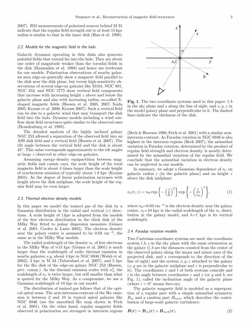
y

z

Α

b

s

x,l

Fig. 1. The two coordinate systems used in this paper: l, bin the sky plane and s along the line of sight, and x, y, z inthe model galaxy plane and perpendicular to it. The dashedlines indicate the thickness of the disk.

(Beck & Hoernes 1996; Frick et al. 2001) with a similar arm-interarm-contrast. As Faraday rotation in NGC 6946 is alsohighest in the interarm regions (Beck 2007), the azimuthalvariation in Faraday rotation, determined by the product ofregular field strength and electron density, is mostly deter-mined by the azimuthal variation of the regular field. Weconclude that the azimuthal variation in electron densitycan be neglected in our models.

In summary, we adopt a Gaussian dependence of ne ongalactic radius r (in the galactic plane) and on height zabove the disk midplane:

ne(r, z) = n0 exp

−( z

h

)2

exp

−(

r

r0

)2

, (1)

where n0=0.03 cm−3 is the electron density near the galaxycenter, r0=10 kpc is the radial scalelength of the ne distri-bution in the galaxy model, and h=1 kpc is its verticalscalelength.

2.4. Faraday rotation models

Two Cartesian coordinate systems are used: the coordinatesystem l, b, s in the sky plane with the same orientation asthe galaxy (l, b are the distances counted from the center ofthe observed galaxy along the major and minor axes of theprojected disk, and s corresponds to the direction of theline of sight) and the system x, y, z attached to the galaxy(x, y are in the galactic midplane and z is perpendicular toit). The coordinates x and l of both systems coincide andi is the angle between coordinates z and s (or y and b, seeFig. 1), called the inclination angle of the galactic plane(where i = 0 means face-on).

The galactic magnetic field is modeled as a superposi-tion of a regular part with a simple azimuthal symmetryBm and a random part Bturb, which describes the contri-bution of large-scale galactic turbulence:

B(r) = Bm(r) + Bturb(r), (2)


Fig. 2. Modeled strength of the regular magnetic field multiplied by the thermal electron density in the galactic midplane(i.e. in the plane x, y) for the field modes m = 0 (ASS), m = 1 (BSS), and m = 2 (QSS) for B = 1.

where r is the radius vector in galactic coordinates, whichwill be written in Cartesian coordinates (x,y,z) or cylindri-

cal ones (r =√

x2 + y2, φ = arctany/x, z).First, the regular part of magnetic field is supposed to be

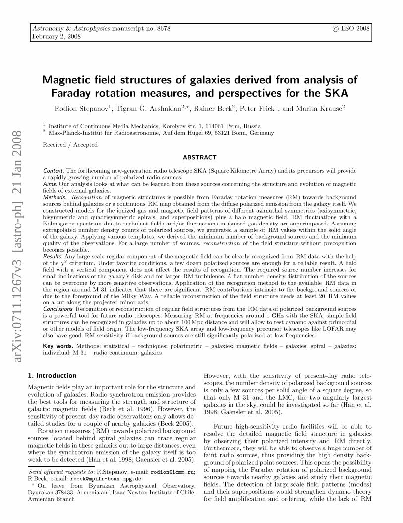
purely horizontal (Bz = 0), parameterized by the pitch an-gle p and the intensity Bm of the corresponding azimuthalmode m (we only consider m = 0, 1, 2, using the notationASS, BSS, and QSS, see Fig. 2). The BSS mode has tworeversals along azimuthal angle, the QSS mode has four re-versals. All modes are symmetric with respect to the diskplane. The strength of the magnetic field in cylindrical co-ordinates is defined as

Bm(r, φ, p) = B cos

(

m

(

ln r

tan p− φ + φ0

))

tanh

(

5r

r0

)

, (3)

where B is the field amplitude (strength) and φ0 the az-imuthal phase of the mode. The tanh term is introducedto suppress the field near the center of the galaxy wherethe spiral field is strongly twisted. Equation (3) does notinclude any decrease in the field strength with radius r andheight z, because the decay in regular field strength is muchslower than that of electron density (see Eq.(1)).

The RM is proportional to the product of the densityof thermal electrons ne and the component of the regularmagnetic field B‖ parallel to the line of sight. Note thatwe cannot separate the contributions of B and ne using theRM data alone and that we can reconstruct only the prod-uct (B‖ ne). As we neglect any azimuthal (e.g. spiral) struc-ture in ne, the small-scale structure in RM is determinedby B, whereas the general radial and vertical decrease inRM is determined by ne. The distribution of this field inthe galactic midplane for m = 0, 1, 2 (ASS, BSS, and QSS)is shown in Fig. 2.

Second, we consider a model in which a vertical field Bz

exists and increases with height z, according to the mag-netic field structure observed in the halos of nearby edge-ongalaxies (see Sect. 2.2). We suppose that the modulus of themagnetic field follows again Eq. (3), but the field lines aretilted with respect to the plane. The tilt angle χ is definedas

χ = χ0 tanhz

2htanh

3r

r0

, (4)

where χ0 = π/4 is the limit of the tilt angle in our modelachieved at r ≈ r0/3, z ≈ 2h. The orientations of magneticfield lines for the ASS model are shown in Fig. 3.

2 4 6 8 10 12

-4

-2

2

4

Fig. 3. Orientation of the halo magnetic field. The boxsketches the region of ionized gas r < r0, −h < z < h.

The magnetic field component B‖ parallel to the lineof sight includes the turbulent (random) magnetic field aswell as the regular one, so that

RM(l, b) = 0.81

∫ ∞

−∞

(Bm(r, p) + Bturb(r)) ne(r)ds. (5)

The turbulent part of magnetic field Bturb should describethe three-dimensional random field with given spectralproperties in the whole range of scales. To avoid full 3-Dsimulations of the random vector field and its contributionto RM, we prefer to model this contribution of the irregu-lar part of magnetic field directly in the RM maps. Thuswe write

RM(l, b) = 0.81

∫ ∞

−∞

Bm(r, p)ne(r)ds + RMturb(l, b), (6)

where we add the random part of the galactic field projectedto the sky plane, i.e. integrated along the line of sight.

RMturb(l, b) is produced in a way that allows for thespectral and spatial distribution of galactic turbulent fields.Vogt & Enßlin (2005) show that by observing a turbulentmagnetic field with a three-dimensional Fourier power-law

spectrum like |B(k)|2 ∼ kα one obtains an RM map, thetwo-dimensional spectrum, from which another power lawfollows | RM(k⊥)|2 ∼ k⊥

β with the slope β = α. Here thehat is used for the notation of the Fourier transform ofany function f(k) =

∫

f(x)eikxdx, k is the 3-D wave vec-tor and k⊥ is the 2-D wave vector, defined in the plane ofthe RM map. It is supposed that the magnetic spectrum


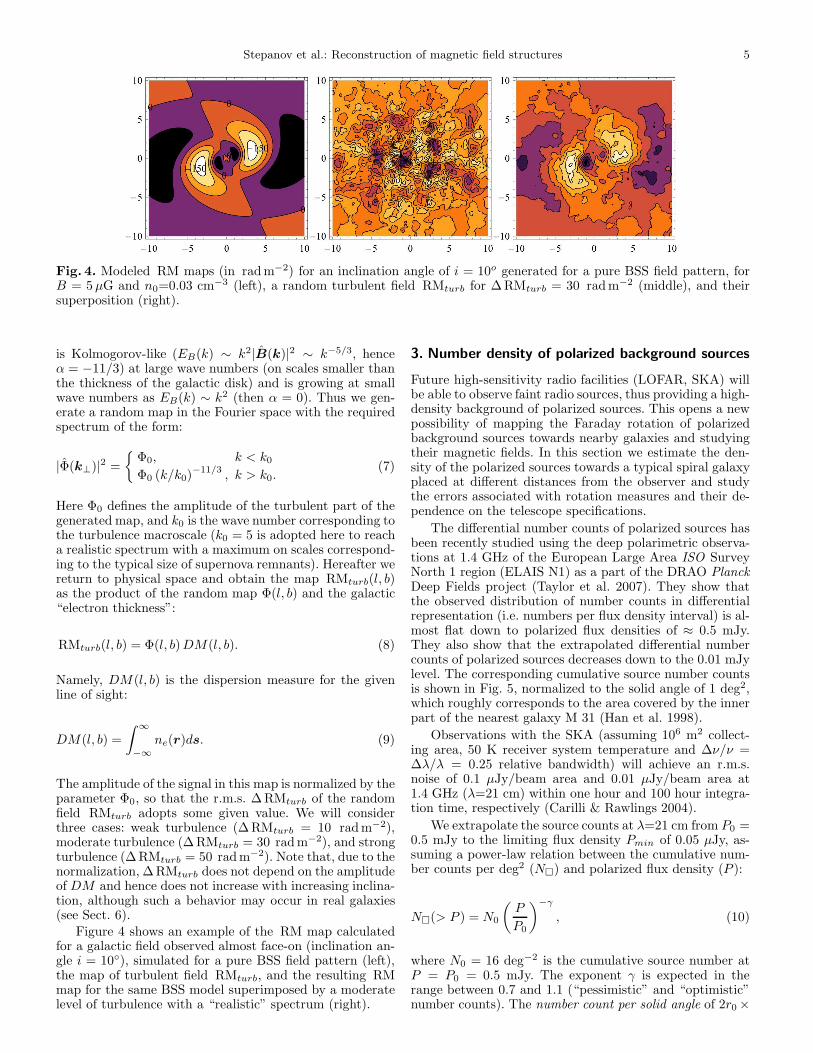
Fig. 4. Modeled RM maps (in rad m−2) for an inclination angle of i = 10o generated for a pure BSS field pattern, forB = 5 µG and n0=0.03 cm−3 (left), a random turbulent field RMturb for ∆RMturb = 30 rad m−2 (middle), and theirsuperposition (right).

is Kolmogorov-like (EB(k) ∼ k2|B(k)|2 ∼ k−5/3, henceα = −11/3) at large wave numbers (on scales smaller thanthe thickness of the galactic disk) and is growing at smallwave numbers as EB(k) ∼ k2 (then α = 0). Thus we gen-erate a random map in the Fourier space with the requiredspectrum of the form:

|Φ(k⊥)|2 =

Φ0, k < k0

Φ0 (k/k0)−11/3 , k > k0.

(7)

Here Φ0 defines the amplitude of the turbulent part of thegenerated map, and k0 is the wave number corresponding tothe turbulence macroscale (k0 = 5 is adopted here to reacha realistic spectrum with a maximum on scales correspond-ing to the typical size of supernova remnants). Hereafter wereturn to physical space and obtain the map RMturb(l, b)as the product of the random map Φ(l, b) and the galactic“electron thickness”:

RMturb(l, b) = Φ(l, b)DM(l, b). (8)

Namely, DM(l, b) is the dispersion measure for the givenline of sight:

DM(l, b) =

∫ ∞

−∞

ne(r)ds. (9)

The amplitude of the signal in this map is normalized by theparameter Φ0, so that the r.m.s. ∆RMturb of the randomfield RMturb adopts some given value. We will considerthree cases: weak turbulence (∆RMturb = 10 rad m−2),moderate turbulence (∆RMturb = 30 rad m−2), and strongturbulence (∆RMturb = 50 rad m−2). Note that, due to thenormalization, ∆RMturb does not depend on the amplitudeof DM and hence does not increase with increasing inclina-tion, although such a behavior may occur in real galaxies(see Sect. 6).

Figure 4 shows an example of the RM map calculatedfor a galactic field observed almost face-on (inclination an-gle i = 10), simulated for a pure BSS field pattern (left),the map of turbulent field RMturb, and the resulting RMmap for the same BSS model superimposed by a moderatelevel of turbulence with a “realistic” spectrum (right).

3. Number density of polarized background sources

Future high-sensitivity radio facilities (LOFAR, SKA) willbe able to observe faint radio sources, thus providing a high-density background of polarized sources. This opens a newpossibility of mapping the Faraday rotation of polarizedbackground sources towards nearby galaxies and studyingtheir magnetic fields. In this section we estimate the den-sity of the polarized sources towards a typical spiral galaxyplaced at different distances from the observer and studythe errors associated with rotation measures and their de-pendence on the telescope specifications.

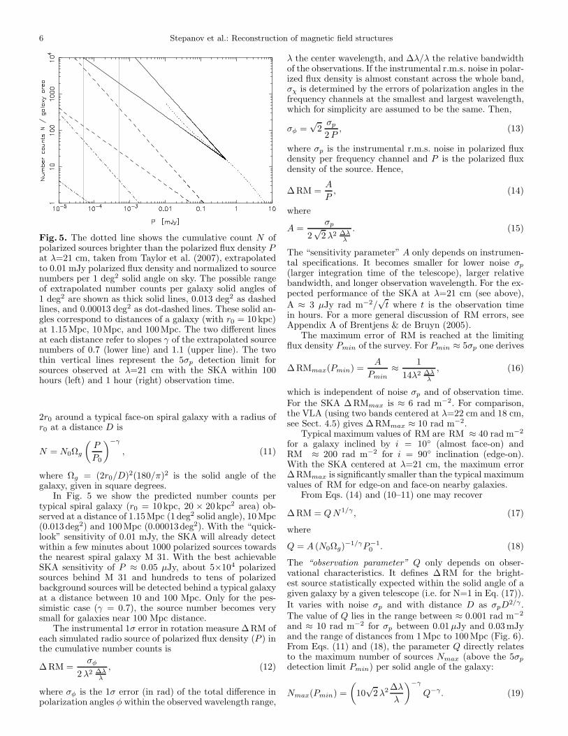
The differential number counts of polarized sources hasbeen recently studied using the deep polarimetric observa-tions at 1.4 GHz of the European Large Area ISO SurveyNorth 1 region (ELAIS N1) as a part of the DRAO PlanckDeep Fields project (Taylor et al. 2007). They show thatthe observed distribution of number counts in differentialrepresentation (i.e. numbers per flux density interval) is al-most flat down to polarized flux densities of ≈ 0.5 mJy.They also show that the extrapolated differential numbercounts of polarized sources decreases down to the 0.01 mJylevel. The corresponding cumulative source number countsis shown in Fig. 5, normalized to the solid angle of 1 deg2,which roughly corresponds to the area covered by the innerpart of the nearest galaxy M 31 (Han et al. 1998).

Observations with the SKA (assuming 106 m2 collect-ing area, 50 K receiver system temperature and ∆ν/ν =∆λ/λ = 0.25 relative bandwidth) will achieve an r.m.s.noise of 0.1 µJy/beam area and 0.01 µJy/beam area at1.4 GHz (λ=21 cm) within one hour and 100 hour integra-tion time, respectively (Carilli & Rawlings 2004).

We extrapolate the source counts at λ=21 cm from P0 =0.5 mJy to the limiting flux density Pmin of 0.05 µJy, as-suming a power-law relation between the cumulative num-ber counts per deg2 (N) and polarized flux density (P ):

N(> P ) = N0

(

P

P0

)−γ

, (10)

where N0 = 16 deg−2 is the cumulative source number atP = P0 = 0.5 mJy. The exponent γ is expected in therange between 0.7 and 1.1 (“pessimistic” and “optimistic”number counts). The number count per solid angle of 2r0 ×


Fig. 5. The dotted line shows the cumulative count N ofpolarized sources brighter than the polarized flux density Pat λ=21 cm, taken from Taylor et al. (2007), extrapolatedto 0.01 mJy polarized flux density and normalized to sourcenumbers per 1 deg2 solid angle on sky. The possible rangeof extrapolated number counts per galaxy solid angles of1 deg2 are shown as thick solid lines, 0.013 deg2 as dashedlines, and 0.00013 deg2 as dot-dashed lines. These solid an-gles correspond to distances of a galaxy (with r0 = 10kpc)at 1.15Mpc, 10Mpc, and 100Mpc. The two different linesat each distance refer to slopes γ of the extrapolated sourcenumbers of 0.7 (lower line) and 1.1 (upper line). The twothin vertical lines represent the 5σp detection limit forsources observed at λ=21 cm with the SKA within 100hours (left) and 1 hour (right) observation time.

2r0 around a typical face-on spiral galaxy with a radius ofr0 at a distance D is

N = N0Ωg

(

P

P0

)−γ

, (11)

where Ωg = (2r0/D)2(180/π)2 is the solid angle of thegalaxy, given in square degrees.

In Fig. 5 we show the predicted number counts pertypical spiral galaxy (r0 = 10kpc, 20 × 20 kpc2 area) ob-served at a distance of 1.15Mpc (1 deg2 solid angle), 10Mpc(0.013deg2) and 100Mpc (0.00013deg2). With the “quick-look” sensitivity of 0.01 mJy, the SKA will already detectwithin a few minutes about 1000 polarized sources towardsthe nearest spiral galaxy M 31. With the best achievableSKA sensitivity of P ≈ 0.05 µJy, about 5×104 polarizedsources behind M 31 and hundreds to tens of polarizedbackground sources will be detected behind a typical galaxyat a distance between 10 and 100 Mpc. Only for the pes-simistic case (γ = 0.7), the source number becomes verysmall for galaxies near 100 Mpc distance.

The instrumental 1σ error in rotation measure ∆RM ofeach simulated radio source of polarized flux density (P ) inthe cumulative number counts is

∆RM =σφ

2 λ2 ∆λλ

, (12)

where σφ is the 1σ error (in rad) of the total difference inpolarization angles φ within the observed wavelength range,

λ the center wavelength, and ∆λ/λ the relative bandwidthof the observations. If the instrumental r.m.s. noise in polar-ized flux density is almost constant across the whole band,σχ is determined by the errors of polarization angles in thefrequency channels at the smallest and largest wavelength,which for simplicity are assumed to be the same. Then,

σφ =√

2σp

2 P, (13)

where σp is the instrumental r.m.s. noise in polarized fluxdensity per frequency channel and P is the polarized fluxdensity of the source. Hence,

∆RM =A

P, (14)

where

A =σp

2√

2 λ2 ∆λλ

. (15)

The “sensitivity parameter” A only depends on instrumen-tal specifications. It becomes smaller for lower noise σp

(larger integration time of the telescope), larger relativebandwidth, and longer observation wavelength. For the ex-pected performance of the SKA at λ=21 cm (see above),A ≈ 3 µJy rad m−2/

√t where t is the observation time

in hours. For a more general discussion of RM errors, seeAppendix A of Brentjens & de Bruyn (2005).

The maximum error of RM is reached at the limitingflux density Pmin of the survey. For Pmin ≈ 5σp one derives

∆RMmax(Pmin) =A

Pmin≈ 1

14λ2 ∆λλ

, (16)

which is independent of noise σp and of observation time.For the SKA ∆RMmax is ≈ 6 rad m−2. For comparison,the VLA (using two bands centered at λ=22 cm and 18 cm,see Sect. 4.5) gives ∆RMmax ≈ 10 rad m−2.

Typical maximum values of RM are RM ≈ 40 rad m−2

for a galaxy inclined by i = 10 (almost face-on) andRM ≈ 200 rad m−2 for i = 90 inclination (edge-on).With the SKA centered at λ=21 cm, the maximum error∆RMmax is significantly smaller than the typical maximumvalues of RM for edge-on and face-on nearby galaxies.

From Eqs. (14) and (10–11) one may recover

∆RM = Q N1/γ , (17)

where

Q = A (N0Ωg)−1/γP−1

0. (18)

The “observation parameter” Q only depends on obser-vational characteristics. It defines ∆RM for the bright-est source statistically expected within the solid angle of agiven galaxy by a given telescope (i.e. for N=1 in Eq. (17)).It varies with noise σp and with distance D as σpD

2/γ .The value of Q lies in the range between ≈ 0.001 rad m−2

and ≈ 10 rad m−2 for σp between 0.01 µJy and 0.03mJyand the range of distances from 1Mpc to 100Mpc (Fig. 6).From Eqs. (11) and (18), the parameter Q directly relatesto the maximum number of sources Nmax (above the 5σp

detection limit Pmin) per solid angle of the galaxy:

Nmax(Pmin) =

(

10√

2λ2∆λ

λ

)−γ

Q−γ . (19)


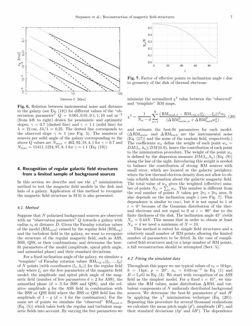
Fig. 6. Relation between instrumental noise and distanceto the galaxy (see Eq. (18)) for different values of the “ob-servation parameter” Q = 0.001, 0.01, 0.1, 1, 10 rad m−2

(from left to right) drawn for pessimistic and optimisticslopes, γ = 0.7 (dashed line) and γ = 1.1 (solid line) forλ = 21 cm, δλ/λ = 0.25. The dotted line corresponds tothe observed slope γ ≈ 1 (see Fig. 5). The numbers ofsources per solid angle of the galaxy corresponding to theabove Q values are Nmax = 462, 92, 18, 4, 1 for γ = 0.7 andNmax = 15411, 1224, 97, 8, 1 for γ = 1.1 (Eq. (19)).

4. Recognition of regular galactic field structures

from a limited sample of background sources

In this section we describe and use the χ2 minimizationmethod to test the magnetic field models in the disk andhalo of a galaxy. Application of this method to recognizethe magnetic field structure in M 31 is also presented.

4.1. Method

Suppose that N polarized background sources are observedwith an “observation parameter” Q towards a galaxy withradius r0 at distance D. Given the Faraday rotation valuesof the model (RMmod) caused by the regular field (RMreg)and the turbulent field in the galaxy, we want to recognizethe structure of the regular magnetic field, such as ASS,BSS, QSS, or their combinations, and determine the best-fit parameters of the model (amplitude, spiral pitch angle,and azimuthal phase) and their standard deviations.

For a fixed inclination angle of the galaxy, we simulate a“template” of Faraday rotation values RMreg, n(ξ1, ..., ξd)of N points (with coordinates (ln, bn)) for the regular fieldonly where ξj are the free parameters of the magnetic fieldmodel: the amplitude and spiral pitch angle of the mag-netic field (number of free parameters d = 2 for ASS), theazimuthal phase (d = 3 for BSS and QSS), and the rel-ative amplitude q for the ASS field in combination withthe BSS or QSS field where the BSS or QSS field has theamplitude of 1 − q (d = 4 for the combination). For thesame set of points we simulate the “observed” RMmod, n

(Eq. (5)) which takes both the regular and turbulent mag-netic fields into account. By varying the free parameters we

0 20 40 60 800.0

0.1

0.2

0.3

0.4

0.5

i

NwN

Fig. 7. Factor of effective points vs inclination angle i dueto geometry of the disk of thermal electrons.

minimize the normalized χ2 value between the “observed”and “template” RM maps,

χ2 =1

Nw − d

N∑

n=1

(RMmod, n − RMreg, n(ξ1, ..., ξd))2wn

(∆RM2

noise,n + ∆RM2

turbw2n)

, (20)

and estimate the best-fit parameters for each model.(∆RMnoise and ∆RMturb are the instrumental noise(Eq. (17)) and the noise of the random field, respectively.)The coefficients wn define the weight of each point wn =DM(ln, bn)/DM(0, 0), hence the contribution of each pointto the minimization procedure. The weight of the point wn

is defined by the dispersion measure DM(ln, bn) (Eq. (9))along the line of the sight. Introducing this weight is neededto balance the contribution of strong RM sources withsmall error, which are located at the galactic periphery,where the low thermal electron density does not allow to ob-tain reliable information about the galactic magnetic field.The total value of wn gives the weighted (effective) num-ber of points Nw =

∑

n wn. This number is different fromthe real number of points N taken per 2r0 × 2r0 area. Italso depends on the inclination angle i (see Fig. 7). Thisdependence is similar to cos i, but it is not equal to 1 ati = 0 because of the Gaussian distribution of the ther-mal electrons and not equal to 0 at i = 90 due to thefinite thickness of the disk. The inclination angle 45 yieldsNw = 0.44N . This means that in order to obtain at leastNw = 4 we need a minimum of N = 10.

This method is suited for simple field structures and arelatively small number of RM points allowing the limitednumber of parameters to be fitted. In the case of compli-cated field structures and/or a large number of RM points,a full reconstruction should be attempted (Sect. 5).

4.2. Fitting the simulated data

Throughout this paper we use typical values of r0 = 10kpc,h = 1 kpc, p = 20, ne = 0.03 cm−3 in Eq. (1) andB = 5 µG in Eq. (3). We start with recognition of an ASSfield as the simplest model. For a fixed i = 45, we sim-ulate the RM values, noise distribution ∆RM, and tur-bulent components of N uniformly distributed backgroundsources. We determine the best-fit parameters p′ and B′

by applying the χ2 minimization technique (Eq. (20)).Repeating this procedure for several thousand realizationswe calculate the mean pitch angle (p′), amplitude (B′), andtheir standard deviations (δp′ and δB′). The dependence


Fig. 8. ASS field model: mean values (figures in left col-umn) and standard deviations (figures in right column) ofpitch angles p′ and amplitudes B′ (given in µG) for fixedvalues of h = 1 kpc, p = 20, B = 5 µG, i = 45 and assum-ing the pessimistic case of number counts (γ = 0.7). N isthe real number of points observed within the solid angle ofthe galaxy and Q is the observation parameter (Eq. (18)).

of the statistical properties of the fitted parameters on thenumber N of sources per solid angle of the galaxy and onQ are shown in Fig. 8.

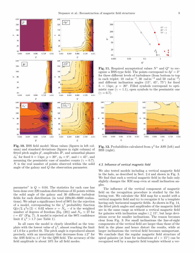
The simulated value of p′ is in good agreement with thevalue p = 20 used for the model calculation over a widerange of N and Q. However, the standard deviation of δp′ isquite small only for low values of Q and for large numbersN . The amplitude B′ is well defined, too. The behaviour ofδB′ is the same as for δp′. The standard deviation diagramsshow that there is a certain value of Q below which betterobservations do not improve the result of fitting. The sameis valid beyond a certain value of N . For example, for thelevel of δp′ = 3 no more than 36 sources observed withQ = 0.2 are needed, or no better values than Q = 0.05when observing 21 sources. Hence, the fitting problem canbe characterized by two asymptotic values N∗ and Q∗, pro-vided that the accuracy of the fitting is fixed. (For the givenexample one obtains N∗ = 21 and Q∗ = 0.2.) These twoparameters define the required quality of observations.

In Fig. 9 we show the dependence of asymptotic param-eters N∗ and Q∗ on the level of turbulence and pitch angleof the observed galaxy for optimistic and pessimistic valuesof γ. The required level of accuracy is fixed at δp′ = 3.

We conclude that, in the case of the pessimistic slope,one needs observations with smaller Q, hence smaller noiseσp, which requires a longer integration time. An increase inthe number of sources (for a fixed noise value σp) does nothelp. This can be explained by the fact that for low valuesof γ additional sources are fainter, have higher errors, anddo not improve the result. The optimistic evaluation of γessentially increases the values of Q∗, but slightly affects

á

á

à

õ

õ

õ

ô

ô

ô

óó

ó

òò

ò

15° - á45° - õ75° - ó

0.001 0.01 0.1 1

10

20

50

100

200

500

Q*

N*

Fig. 9. Required asymptotic values N∗ and Q∗ to recognizean ASS-type field. The points correspond to δp′ = 3 forthree different levels of turbulence (from bottom to top ineach triplet: 10 rad m−2, 30 rad m−2 and 50 rad m−2) andfor different inclination angles (15, 45, 75) for fixed h =1 kpc, p = 20. Filled symbols correspond to the optimisticcase (γ = 1.1), open symbols to the pessimistic one (γ =0.7).

the values of N∗. As expected, the result of fitting stronglydepends on the level of turbulence of the galactic field: inthe case of intense turbulence one needs more points andsmaller Q (longer observations or a more sensitive instru-ment). The dependence on turbulence becomes dramaticfor weakly inclined (face-on) galaxies – the reliable fittingrequires a huge number of sources under any value of γ.

The same simulations are performed for the BSS andQSS models. An additional free parameter (the phase φ)is accounted for, but, in general, the results are similar tothose obtained for the ASS model (see Figs. 10 and 11).Comparing Figs. 9 and 11 (or Figs. 8 and 10), we con-clude that the bisymmetric field can be easier recognized(it requires fewer points and higher Q for the same accu-racy of pitch angle definition) and weakly depends on theturbulent component of magnetic field. The BSS field hasbetter chances of being recognized in slightly inclined galax-ies. However, with values of N , the BSS model has a higherprobability of being false than the ASS model (see Fig. 12).

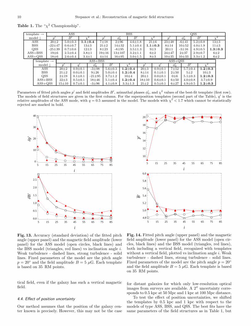
The dependence of the fitting accuracy on the incli-nation angle is shown in Fig. 13. We learn that face-ongalaxies always pose more problems for recognition of thefield structure. The accuracy of the ASS or BSS recogni-tion increases monotonically with inclination angle due tostronger line-of-sight components of the regular field. Forinclination angles ≥ 70, the number of effective points de-creases. Furthermore, RM becomes sensitive to fluctuationsof the regular field, e.g. due to spiral arms (see Sect. 6), sothat the reconstruction method (Sect. 5) is recommendedfor strongly inclined galaxies.

To illustrate the potential of identification of differentmodels of the regular magnetic field, using a set of tem-plates, we present in Table 1 the results of recognition un-der a moderate level of galactic turbulence (∆RMturb =30 rad m−2) for a sample of 35 sources. The models of mag-netic field structures with fixed parameters of p = 20,φ0 = 0, and B = 5 µG are used. The assumed level ofgalactic turbulence is ∆RMturb = 30 rad m−2, the incli-nation of the galaxy’s disk is 45, the slope of the sourcecounts γ = 0.7 (“pessimistic case”), and the “observation


Fig. 10. BSS field model: Mean values (figures in left col-umn) and standard deviations (figures in right column) offitted pitch angles p′, amplitudes B′, and azimuthal phases

φ0

′for fixed h = 1 kpc, p = 20, φ0 = 0, and i = 45, and

assuming the pessimistic case of number counts (γ = 0.7).N is the real number of points observed within the solidangle of the galaxy and Q the observation parameter.

parameter” is Q = 0.04. The statistics for each case hasbeen done over 220 random distributions of 35 points withinthe solid angle of the galaxy and 30 different turbulentfields for each distribution (in total 220x30=6600 realiza-tions). We adopt a significance level of 98% for the rejectionof a model, corresponding to the χ2 probability functionQ(ν/2, χ2ν/2) < 0.02 where ν = Nw − d is the weightednumber of degrees of freedom (Eq. (20)) and Nw ≃ 27 fori = 45 (Fig. 7). A model is rejected at the 98% confidencelimit if χ2 > 1.7 (see Table 1).

In all cases the model is clearly identified as the tem-plate with the lowest value of χ2, almost reaching the limitof 1.0 for a perfect fit. The pitch angle is reproduced almostprecisely, with an uncertainty that decreases from ±2 forthe ASS field to ±1 for the QSS field. The accuracy of thefield amplitude is about 10% for all field modes.

á

á

à

à

õõ

õ

ôô

ô

ó

ó

ó

ò

ò

ò

15° - á45° - õ75° - ó

0.001 0.01 0.1 1

10

20

50

100

200

500

Q*

N*

Fig. 11. Required asymptotical values N∗ and Q∗ to rec-ognize a BSS-type field. The points correspond to δp′ = 3

for three different levels of turbulence (from bottom to topin each triplet: 10 rad m−2, 30 rad m−2 and 50 rad m−2)and different inclination angles (15, 45, 75) for fixedh = 1 kpc, p = 20. Filled symbols correspond to opti-mistic case (γ = 1.1), open symbols to the pessimistic one(γ = 0.7).

0.5

0.55

0.6

0.65

0.70.75

0.001 0.009 0.081 0.729 6.56110

20

40

80

160

320

640

Q

N

0.55

0.550.55

0.6

0.65

0.70.75

0.80.850.90.951

0.001 0.009 0.081 0.729 6.56110

20

40

80

160

320

640

QN

Fig. 12. Probabilities calculated from χ2 for ASS (left) andBSS (right).

4.3. Influence of vertical magnetic field

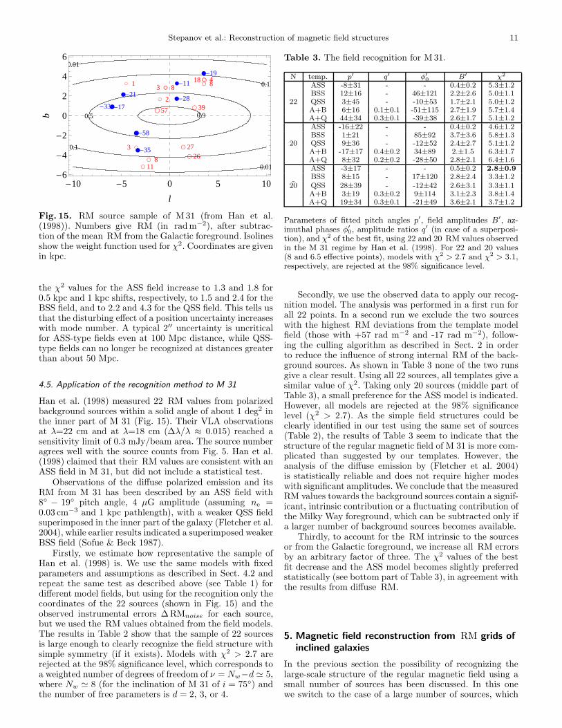
We also tested models including a vertical magnetic fieldin the halo, as described in Sect. 2.4 and shown in Fig. 3.We find that such a vertical magnetic field in the halo onlyslightly changes the RM map even at small inclination an-gles.

The influence of the vertical component of magneticfield on the recognition procedure is studied by the fol-lowing test. We calculate the RM map for a model with avertical magnetic field and try to recognize it by a templatehaving only horizontal magnetic fields. As shown in Fig. 14,the fitted pitch angles and amplitudes of the magnetic fieldare in the same range as without a vertical magnetic fieldfor galaxies with inclination angles i & 15, but large devi-ations occur for smaller inclinations. The reason becomesclear from Fig. 3: For small inclinations the line-of-sightcomponents of the vertical field are larger than those of thefield in the plane and hence distort the results, while atlarger inclinations the vertical field becomes unimportant.We conclude that the regular magnetic field structure ofspiral galaxies (at least for inclinations of i > 15) can berecognized well by a magnetic field template without a ver-


Table 1. The “χ2 Championship”.

template → ASS BSS QSSmodel ↓ p′ B′ χ2 p′ φ′

0B′ χ2 p′ φ′

0B′ χ2

ASS 20±2 5.0±0.3 1.1±0.4 7±18 2±96 4.6±1.8 21±6 23±48 -6±41 5.2±0.8 13±3BSS -22±47 0.6±0.7 13±3 21±2 14±32 5.1±0.4 1.1±0.3 8±14 10±52 4.0±1.9 11±3QSS -25±39 0.7±0.6 12±3 8±23 -8±95 3.5±1.3 9±3 20±1 -3±16 4.9±0.5 1.3±0.3

ASS+BSS 19±6 2.5±0.4 3.8±1 19±16 13±107 3.2±1.1 6±2 24±47 2±37 2.9±0.7 6±2ASS+QSS 18±6 2.6±0.4 3.4±1 4±14 16±95 3.0±1.5 8±3 10±35 10±33 3.3±1.2 6±2

template → ASS+BSS ASS+QSSmodel ↓ p′ q′ φ′

0B′ χ2 p′ q′ φ′

0B′ χ2

ASS 20±2 0.9±0.1 -3±98 5.6±0.3 1.2±0.4 20±3 0.9±0.1 7±52 5.7±0.4 1.2±0.3

BSS 21±2 0.0±0.1 9±26 5.0±0.4 1.2±0.4 8±14 0.1±0.1 2±50 5±2 10±3QSS 2±19 0.1±0.1 -21±95 3.7±1.2 10±4 20±1 0.0±0.1 0±6 5.1±0.3 1.2±0.3

ASS+BSS 22±3 0.5±0.1 18±46 5.1±0.4 1.2±0.4 18±10 0.6±0.1 6±50 4.0±0.8 3.7±0.9ASS+QSS 15±10 0.7±0.1 -3±96 4.1±0.8 3.3±1.3 21±2 0.5±0.1 6±27 4.9±0.5 1.2±0.3

Parameters of fitted pitch angles p′ and field amplitudes B′, azimuthal phases φ′

0, and χ2 values of the best-fit template (first row).The models of field structures are given in the first column. For the superposition templates (second part of the Table), q′ is therelative amplitudes of the ASS mode, with q = 0.5 assumed in the model. The models with χ2 < 1.7 which cannot be statisticallyrejected are marked in bold.

ç

çç

ç ç ç ç ç çç

ç

ç

ç

çç ç ç ç ç

ò

òò

ò

ò

ò

òò ò ò ò

ò

5 15 25 35 45 55 65 75 850

10

20

30

40

i

∆p’

ç

çç

ç ç ç ç ç ç

ç

ç

ç

çç ç

çç ç

ò

òò

òò ò ò ò

ò

ò

ò

ò

ò

òò

ò òò

5 15 25 35 45 55 65 75 850.0

0.5

1.0

1.5

2.0

2.5

i

∆B

’

Fig. 13. Accuracy (standard deviation) of the fitted pitchangle (upper panel) and the magnetic field amplitude (lowerpanel) for the ASS model (open circles, black lines) andthe BSS model (triangles, red lines) vs inclination angle i.Weak turbulence - dashed lines, strong turbulence - solidlines. Fixed parameters of the model are the pitch anglep = 20 and the field amplitude B = 5 µG. Each templateis based on 35 RM points.

tical field, even if the galaxy has such a vertical magneticfield.

4.4. Effect of position uncertainty

Our method assumes that the position of the galaxy cen-ter known is precisely. However, this may not be the case

ç

çç ç ç ç ç ç

ç

çç

çç

ç

çç

ç çò

òò ò ò ò ò ò ò

ò

ò

ò

ò òò ò ò ò

5 15 25 35 45 55 65 75 85

10

12

14

16

18

20

i

p’

ç

çç

ç ç

ç ç ç ç

ç

ç

ç

ç

çç ç

çç

òò ò ò ò ò ò ò ò

ò

òò

ò òò ò ò ò

5 15 25 35 45 55 65 75 854.8

5.0

5.2

5.4

5.6

5.8

6.0

i

B’

Fig. 14. Fitted pitch angle (upper panel) and the magneticfield amplitude (lower panel) for the ASS model (open cir-cles, black lines) and the BSS model (triangles, red lines),both including a vertical field, recognized with templateswithout a vertical field, plotted vs inclination angle i. Weakturbulence - dashed lines, strong turbulence - solid lines.Fixed parameters of the model are the pitch angle p = 20

and the field amplitude B = 5 µG. Each template is basedon 35 RM points.

for distant galaxies for which only low-resolution opticalimages from surveys are available. A 2′′ uncertainty corre-sponds to 0.5 kpc at 50 Mpc and 1 kpc at 100 Mpc distance.

To test the effect of position uncertainties, we shiftedthe templates by 0.5 kpc and 1 kpc with respect to themodels of type ASS, BSS, and QSS. The best fits have thesame parameters of the field structures as in Table 1, but


0.01

0.01

0.1

0.1

0.5 0.9

æ-19ç18 ç 4ç 8æ-11

ç 8ç3

ç 39æ-28ç 2

ç 1

ç57

æ-21

ç 27ç 26

æ-17æ-33

æ-58

ç3æ-35ç 8ç 11

-10 -5 0 5 10-6

-4

-2

0

2

4

6

l

b

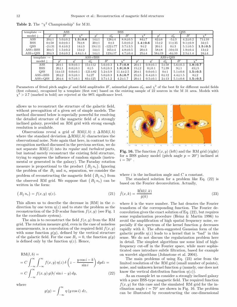
Fig. 15. RM source sample of M 31 (from Han et al.(1998)). Numbers give RM (in rad m−2), after subtrac-tion of the mean RM from the Galactic foreground. Isolinesshow the weight function used for χ2. Coordinates are givenin kpc.

the χ2 values for the ASS field increase to 1.3 and 1.8 for0.5 kpc and 1 kpc shifts, respectively, to 1.5 and 2.4 for theBSS field, and to 2.2 and 4.3 for the QSS field. This tells usthat the disturbing effect of a position uncertainty increaseswith mode number. A typical 2′′ uncertainty is uncriticalfor ASS-type fields even at 100 Mpc distance, while QSS-type fields can no longer be recognized at distances greaterthan about 50 Mpc.

4.5. Application of the recognition method to M 31

Han et al. (1998) measured 22 RM values from polarizedbackground sources within a solid angle of about 1 deg2 inthe inner part of M 31 (Fig. 15). Their VLA observationsat λ=22 cm and at λ=18 cm (∆λ/λ ≈ 0.015) reached asensitivity limit of 0.3 mJy/beam area. The source numberagrees well with the source counts from Fig. 5. Han et al.(1998) claimed that their RM values are consistent with anASS field in M 31, but did not include a statistical test.

Observations of the diffuse polarized emission and itsRM from M 31 has been described by an ASS field with8 − 19 pitch angle, 4 µG amplitude (assuming ne =0.03 cm−3 and 1 kpc pathlength), with a weaker QSS fieldsuperimposed in the inner part of the galaxy (Fletcher et al.2004), while earlier results indicated a superimposed weakerBSS field (Sofue & Beck 1987).

Firstly, we estimate how representative the sample ofHan et al. (1998) is. We use the same models with fixedparameters and assumptions as described in Sect. 4.2 andrepeat the same test as described above (see Table 1) fordifferent model fields, but using for the recognition only thecoordinates of the 22 sources (shown in Fig. 15) and theobserved instrumental errors ∆RMnoise for each source,but we used the RM values obtained from the field models.The results in Table 2 show that the sample of 22 sourcesis large enough to clearly recognize the field structure withsimple symmetry (if it exists). Models with χ2 > 2.7 arerejected at the 98% significance level, which corresponds toa weighted number of degrees of freedom of ν = Nw−d ≃ 5,where Nw ≃ 8 (for the inclination of M 31 of i = 75) andthe number of free parameters is d = 2, 3, or 4.

Table 3. The field recognition for M 31.

N temp. p′ q′ φ′

0B′ χ2

ASS -8±31 - - 0.4±0.2 5.3±1.2BSS 12±16 - 46±121 2.2±2.6 5.0±1.1

22 QSS 3±45 - -10±53 1.7±2.1 5.0±1.2A+B 6±16 0.1±0.1 -51±115 2.7±1.9 5.7±1.4A+Q 44±34 0.3±0.1 -39±38 2.6±1.7 5.1±1.2ASS -16±22 - - 0.4±0.2 4.6±1.2BSS 1±21 - 85±92 3.7±3.6 5.8±1.3

20 QSS 9±36 - -12±52 2.4±2.7 5.1±1.2A+B -17±17 0.4±0.2 34±89 2.±1.5 6.3±1.7A+Q 8±32 0.2±0.2 -28±50 2.8±2.1 6.4±1.6ASS -3±17 - - 0.5±0.2 2.8±0.9

BSS 8±15 - 17±120 2.8±2.4 3.3±1.220 QSS 28±39 - -12±42 2.6±3.1 3.3±1.1

A+B 3±19 0.3±0.2 9±114 3.1±2.3 3.8±1.4A+Q 19±34 0.3±0.1 -21±49 3.6±2.1 3.7±1.2

Parameters of fitted pitch angles p′, field amplitudes B′, az-imuthal phases φ′

0, amplitude ratios q′ (in case of a superposi-tion), and χ2 of the best fit, using 22 and 20 RM values observedin the M 31 regime by Han et al. (1998). For 22 and 20 values(8 and 6.5 effective points), models with χ2 > 2.7 and χ2 > 3.1,respectively, are rejected at the 98% significance level.

Secondly, we use the observed data to apply our recog-nition model. The analysis was performed in a first run forall 22 points. In a second run we exclude the two sourceswith the highest RM deviations from the template modelfield (those with +57 rad m−2 and -17 rad m−2), follow-ing the culling algorithm as described in Sect. 2 in orderto reduce the influence of strong internal RM of the back-ground sources. As shown in Table 3 none of the two runsgive a clear result. Using all 22 sources, all templates give asimilar value of χ2. Taking only 20 sources (middle part ofTable 3), a small preference for the ASS model is indicated.However, all models are rejected at the 98% significancelevel (χ2 > 2.7). As the simple field structures could beclearly identified in our test using the same set of sources(Table 2), the results of Table 3 seem to indicate that thestructure of the regular magnetic field of M 31 is more com-plicated than suggested by our templates. However, theanalysis of the diffuse emission by (Fletcher et al. 2004)is statistically reliable and does not require higher modeswith significant amplitudes. We conclude that the measuredRM values towards the background sources contain a signif-icant, intrinsic contribution or a fluctuating contribution ofthe Milky Way foreground, which can be subtracted only ifa larger number of background sources becomes available.

Thirdly, to account for the RM intrinsic to the sourcesor from the Galactic foreground, we increase all RM errorsby an arbitrary factor of three. The χ2 values of the bestfit decrease and the ASS model becomes slightly preferredstatistically (see bottom part of Table 3), in agreement withthe results from diffuse RM.

5. Magnetic field reconstruction from RM grids of

inclined galaxies

In the previous section the possibility of recognizing thelarge-scale structure of the regular magnetic field using asmall number of sources has been discussed. In this onewe switch to the case of a large number of sources, which


Table 2. The “χ2 Championship” for M 31.

template → ASS BSS QSSmodel ↓ p′ B′ χ2 p′ φ′

0B′ χ2 p′ φ′

0B′ χ2

ASS 20±1 5.0±0.2 1.3±0.6 14±1 128±4 8.8±0.5 84±7 62±6 -5±3 4.2±0.2 71±10BSS 0±58 0.0±0.1 76±8 20±1 0±3 5.0±0.2 1.4±0.6 15±2 11±35 9.1±0.9 34±5QSS -2±31 0.4±0.2 14±3 19±11 -122±77 3.7±3.5 9±2 20±1 0±3 5.1±0.5 1.5±0.5

ASS+BSS 30±5 1.5±0.2 13±2 14±1 165±4 4.8±0.5 20±3 58±8 -10±31 1.9±0.4 13±2ASS+QSS 20±3 2.6±0.2 4.8±1.4 14±1 123±17 4.7±0.4 25±4 58±19 -6±10 2.5±1.4 24±4

template → ASS+BSS ASS+QSSmodel ↓ p′ q′ φ′

0B′ χ2 p′ q′ φ′

0B′ χ2

ASS 20±1 0.9±0.1 15±112 5.6±0.3 1.7±0.8 20±1 0.9±0.1 5±58 5.6±0.3 1.8±0.7

BSS 20±1 0.0±0.1 0±5 5.0±0.3 1.9±0.9 15±2 0±0.1 7±39 9±1 43±5QSS 14±13 0.0±0.1 -121±82 5.2±3.9 11.4±2.5 20±1 0.0±0.1 0±1 5.1±0.6 1.5±0.5

ASS+BSS 20±2 0.5±0.1 5±27 5.0±0.3 1.5±0.7 25±5 0.4±0.1 0±12 4.4±1.5 8±2ASS+QSS 20±4 0.7±0.1 83±125 3.7±1.2 4.2±1.7 20±1 0.5±0.1 2±13 5.1±0.6 1.5±0.5

Parameters of fitted pitch angles p′ and field amplitudes B′, azimuthal phases φ′

0, and χ2 of the best fit for different model fields(first column), recognized by a template (first row) based on the existing sample of 22 sources in the M 31 area. Models withχ2 > 2.7 (marked in bold) are rejected at the 98% significance level.

allows us to reconstruct the structure of the galactic field,without precognition of a given set of simple models. Themethod discussed below is especially powerful for resolvingthe detailed structure of the magnetic field of a stronglyinclined galaxy, provided an RM grid with strong enoughresolution is available.

Observations reveal a grid of RM(l, b) ± ∆RM(l, b)where the standard deviation ∆RM(l, b) characterizes theobservational noise. Note again that here, in contrast to therecognition method discussed in the previous section, we donot separate RM(l, b) into its regular and turbulent parts,but instead merely reconstruct the existing field structure,trying to suppress the influence of random signals (instru-mental or generated in the galaxy). The Faraday rotationmeasure is proportional to the product

(

B‖ ne

)

. Ignoringthe problem of the B‖ and ne separation, we consider the

problem of reconstructing the magnetic field(

B‖ ne

)

from

the observed RM grid. We suppose that(

B‖ ne

)

can bewritten in the form:

(

B‖ ne

)

= f(x, y) η(z). (21)

This allows us to describe the decrease in |RM| in the z-direction by one term η(z) and to state the problem as thereconstruction of the 2-D scalar function f(x, y) (see Fig. 1for the coordinate system).

The aim is to reconstruct the field f(x, y) from the RMgrid. The rotation measure grid, even in the case of noiselessmeasurements, is a convolution of the required field f(x, y)with some function g(y), defined by the vertical structureof the galactic field. For the case Bz = 0, the function g(y)is defined only by the function η(z). Hence,

RM(l, b) =

= C

∫ ∞

−∞

∫ ∞

−∞

f(x, y) η(z) δ

(

z − y cos i − b

sin i

)

dydz =

= C

∫ ∞

−∞

f(x, y) g(b/ sin i − y) dy, (22)

where

g(y) =

∫ ∞

−∞

η (y cos i) dz,

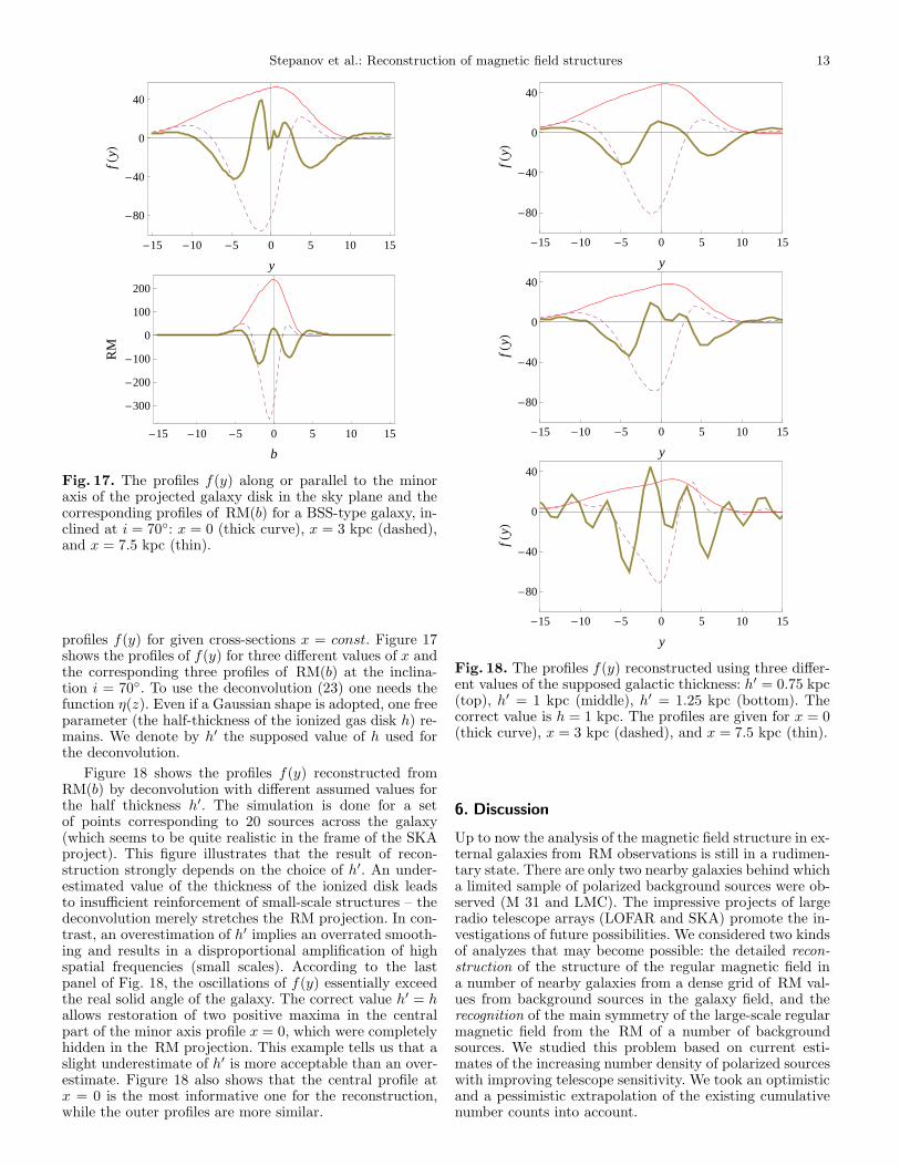
Fig. 16. The function f(x, y) (left) and the RM grid (right)for a BSS galaxy model (pitch angle p = 20) inclined ati = 70 .

where i is the inclination angle and C a constant.The standard solution for a problem like Eq. (22) is

based on the Fourier deconvolution. Actually,

f(x, k) =RM(l, k)

g(k)(23)

where k is the wave number. The hat denotes the Fouriertransform of the corresponding function. The Fourier de-convolution gives the exact solution of Eq. (22), but requiressome regularization procedure (Heinz & Martin 1996) toavoid the amplification of high spatial frequency noise, es-pecially if the spectrum of the kernel function g decreasesrapidly with k. The often-suggested Gaussian form of thegalactic profile η(z) leads to a kernel that is “bad” in thissense. We do not discuss the regularization problem herein detail. The simplest algorithms use some kind of high-frequency cut-off in the Fourier space, while more sophis-ticated ones introduce subtle filtration, based for exampleon wavelet algorithms (Johnstone et al. 2004).

The main problems of using Eq. (23) arise from thelimited resolution of the RM grid (small number of points),noise, and unknown kernel function g (namely, one does notknow the vertical distribution function η(z)).

As an example let us consider a strongly inclined galaxywith a pure BSS-type magnetic field. The required functionf(x, y) for this case and the simulated RM grid for the in-clination angle i = 70 are shown in Fig. 16. The problemcan be illustrated by reconstructing the one-dimensional


-15 -10 -5 0 5 10 15

-80

-40

0

40

y

fHyL

-15 -10 -5 0 5 10 15

-300

-200

-100

0

100

200

b

RM

Fig. 17. The profiles f(y) along or parallel to the minoraxis of the projected galaxy disk in the sky plane and thecorresponding profiles of RM(b) for a BSS-type galaxy, in-clined at i = 70: x = 0 (thick curve), x = 3 kpc (dashed),and x = 7.5 kpc (thin).

profiles f(y) for given cross-sections x = const. Figure 17shows the profiles of f(y) for three different values of x andthe corresponding three profiles of RM(b) at the inclina-tion i = 70. To use the deconvolution (23) one needs thefunction η(z). Even if a Gaussian shape is adopted, one freeparameter (the half-thickness of the ionized gas disk h) re-mains. We denote by h′ the supposed value of h used forthe deconvolution.

Figure 18 shows the profiles f(y) reconstructed fromRM(b) by deconvolution with different assumed values forthe half thickness h′. The simulation is done for a setof points corresponding to 20 sources across the galaxy(which seems to be quite realistic in the frame of the SKAproject). This figure illustrates that the result of recon-struction strongly depends on the choice of h′. An under-estimated value of the thickness of the ionized disk leadsto insufficient reinforcement of small-scale structures – thedeconvolution merely stretches the RM projection. In con-trast, an overestimation of h′ implies an overrated smooth-ing and results in a disproportional amplification of highspatial frequencies (small scales). According to the lastpanel of Fig. 18, the oscillations of f(y) essentially exceedthe real solid angle of the galaxy. The correct value h′ = hallows restoration of two positive maxima in the centralpart of the minor axis profile x = 0, which were completelyhidden in the RM projection. This example tells us that aslight underestimate of h′ is more acceptable than an over-estimate. Figure 18 also shows that the central profile atx = 0 is the most informative one for the reconstruction,while the outer profiles are more similar.

-15 -10 -5 0 5 10 15

-80

-40

0

40

y

fHyL

-15 -10 -5 0 5 10 15

-80

-40

0

40

y

fHyL

-15 -10 -5 0 5 10 15

-80

-40

0

40

y

fHyL

Fig. 18. The profiles f(y) reconstructed using three differ-ent values of the supposed galactic thickness: h′ = 0.75 kpc(top), h′ = 1 kpc (middle), h′ = 1.25 kpc (bottom). Thecorrect value is h = 1 kpc. The profiles are given for x = 0(thick curve), x = 3 kpc (dashed), and x = 7.5 kpc (thin).

6. Discussion

Up to now the analysis of the magnetic field structure in ex-ternal galaxies from RM observations is still in a rudimen-tary state. There are only two nearby galaxies behind whicha limited sample of polarized background sources were ob-served (M 31 and LMC). The impressive projects of largeradio telescope arrays (LOFAR and SKA) promote the in-vestigations of future possibilities. We considered two kindsof analyzes that may become possible: the detailed recon-struction of the structure of the regular magnetic field ina number of nearby galaxies from a dense grid of RM val-ues from background sources in the galaxy field, and therecognition of the main symmetry of the large-scale regularmagnetic field from the RM of a number of backgroundsources. We studied this problem based on current esti-mates of the increasing number density of polarized sourceswith improving telescope sensitivity. We took an optimisticand a pessimistic extrapolation of the existing cumulativenumber counts into account.


In the first part of the paper, we studied the possibilityof recognizing the large-scale regular component of the mag-netic field with a simple symmetry using a straightforwardtesting by templates, which correspond to axisymmetric,bisymmetric, and quadrisymmetric modes, or their super-positions, and applying the χ2 criterium for evaluating thereliability of the different modes. We showed that, if a sym-metric part indeed exists in the analyzed field (even mixedwith a relatively strong turbulent field), dozens of sourcesprovide a good chance of a reliable recognition. These tem-plates can be even successfully applied if the disk field is ac-companied by an X-shaped vertical field as found in nearbygalaxies observed almost edge-on. The result strongly de-pends on the quality of the observations, the flux densityof the sources, and their number density distribution.

Our results show that regular magnetic fields of sim-ple azimuthal symmetry (modes), like axisymmetric (ASS),bisymmetric (BSS), and quadrisymmetric spiral fields(QSS), and superpositions of these, can be recognized withRM values from a number of background sources depend-ing on the inclination of the galaxy’s disk, the level of RMturbulence in the galaxy, and the slope of the number den-sity distribution of the polarized sources. The fitted pa-rameters are the spiral pitch angle, the amplitude of theregular field strength, and the phase (for non-axisymmetricfields). The typical accuracies achieved for the fitted pa-rameters are ±(1 − 4) for the pitch angle and ±10% forthe field amplitude. Under the favorite conditions, 10 − 30sources are already reliable enough to recognize the fieldstructure. However, the unknown internal RM of the back-ground sources themselves may require a larger number ofmeasured sources in order to statistically average out thecontribution of internal RM, or to be able to apply a cullingalgorithm, as mentioned in Sect. 2.

The regular field of a higher order of symmetry can beeasier recognized; i.e. it requires fewer points and shorterobservation time for the same accuracy of the fitted pitchangle definition and is less affected by the turbulent compo-nent of RM. The BSS and QSS fields seem to have betterchances of being recognized in slightly inclined galaxies.However, the smaller required N∗ and the larger number ofparameters for the higher mode decreases the reliability ofthe recognition.

The dependence on turbulence becomes dramatic forweakly inclined (almost face-on) galaxies – a reliable fittingrequires a huge number of sources. This problem may occurespecially for small, slowly rotating galaxies with a highrate of star formation, where the large-scale regular field isexpected to be weaker than the turbulent field (Beck et al.1996). Interactions or ram pressure may also enhance theturbulent field and mask any large-scale pattern in the RMdistribution.

In our models we did not consider deviations of the reg-ular field structure from simple azimuthal modes, e.g. dueto spiral arms or additional field reversals. These wouldlead to further RM fluctuations that may become large forstrongly inclined galaxies and hence decrease the accuracyof the fits. Strong RM fluctuations have been observed nearthe plane of the Milky Way (Brown et al. 2007).

For our test case M 31, the best case of a dominat-ing field mode (ASS) so far, the available RM data frompolarized background sources confirm the results from theanalysis of RM data from the diffuse emission of M 31(Sect. 4.5) if the RM errors are increased to account for

the RM contributions intrinsic to the sources or from theforeground in the Milky Way. A larger number of sourcesis needed for proper subtraction of these effects. However,it is possible that higher field modes exist and will preventa clear result even in case of a greater source number.

The detection of the ASS mode in M 31 from RM ofbackground sources also indicates that this mode is sym-metric with respect to the plane (mode S0) because RMin a strongly inclined galaxy hosting an A0 mode shouldreverse above and below the plane. The RM amplitude ofpolarized sources behind a S0-type field should be twicelarger than that from the RM map of the diffuse polarizedemission from the galaxy itself, which has to be confirmedwith more sensitive data.

For many galaxies no strongly dominating field modecan be expected. A high χ2 value, which does not decreasewith increasing source number, would indicate that the fieldstructure is more complicated than a superposition of a fewsimple modes or that the turbulent field is stronger than theregular field. In this case, our reconstruction method shouldbe applied, because it does not need a “precognition” tem-plate but needs a higher density of RM sources and hencedeeper observations.

Observations provide the 2-D projection of the product(B|| ne). Interpretation of this projection can by impededby a vertical magnetic field Bz, but the contribution of thisfield is not crucial in the case of symmetrically tilted fields.If the inclination angle increases, the RM grid is entirelydominated by the horizontal field, but another problemarises: the smoothing of detailed structures (of the size of aspiral arm) due to their superposition in a highly inclinedprojection. In other words, the function f(x, y) describingthe field structure in the galaxy’s plane is convolved by asmoothing function, defined by the vertical profile of thegalaxy. Provided a universal shape of the profile exists, onecan apply the deconvolution technique to restore the struc-ture of the magnetic field in the galaxy’s plane. In principle,this method works for any field structure.

The reconstruction method is superior for strongly in-clined galaxies (about 70 and more) and is successful ifa large sample of sources is available. At least about 20sources are required for one cut along the minor galac-tic axis (or ∼ 1200 sources within the solid angle coveredby the galaxy) to reconstruct the spiral arms in a spi-ral galaxy. The number of points increases if the scale ofreconstructed details decreases, following the well-knownKotelnikov–Nyquist relation.

Note that the reconstruction procedure can be appliedto the RM obtained from the diffusive polarized emission ofthe galaxy itself, but this would require the deconvolutionof a more complicated integral equation than Eq. (22). Onthe other hand, the recognition method also works for acontinuous RM map obtained from the diffuse polarizedemission.

Finally, we wish to point out that little is known aboutthe statistical properties of the RM contributions intrin-sic to the background sources and of the contribution ofsmall-scale RM inhomogeneities in the foreground of theMilky Way. Large, nearby galaxies will suffer most fromfluctuations in the foreground. Another uncertainty are de-polarization effects within the background sources, or inthe foreground of the galaxy or the Milky Way, if the an-gular extent of a source is greater than the angular tur-bulence scale in the foreground medium. Depolarization of


background sources in the LMC were detected by Gaensleret al. (2005). The latter depolarization effect increases withdistance because larger turbulence scales can contribute.Both depolarization effects, internal and external, dependon angular resolution and on observation frequency. No sta-tistical data are available yet. Further investigations in thisdirection may modify the number of sources required for areliable recognition.

7. Application to LOFAR and SKA

The reconstruction of magnetic field structures of stronglyinclined spiral galaxies is possible for a sample of ≥ 1200RM sources. This would require a sensitivity of the SKAat 1.4 GHz of ≈ 0.5 − 5 µJy (or integration time less thanone hour) for galaxies at distances of about one Mpc. Thefield structures of galaxies at about 10 Mpc distance can bereconstructed with tens to a hundred hours of integrationtime.

The results for the recognition method presented in thispaper are very promising for future observations with theSKA of background sources behind galaxies that are toofaint to be observed directly by their extended polarizedemission. Simple field structures can be recognized with theSKA at 1.4 GHz (21 cm) with an “observation parameter”Q ≈ 1. This needs a σp ≈ 0.2 µJy for galaxies at 30 Mpcdistance and σp ≈ 0.015 µJy for galaxies at 100 Mpc dis-tance. These sensitivities can be achieved within 15 min and100 h observation time, respectively, assuming that polar-ization calibration of the SKA is possible down to such lowflux-density levels.

Let us estimate the number of spiral galaxies forwhich one can reconstruct or recognize the magnetic fields.Marinoni et al. (1999) estimate the mean number of galax-ies (≃ 0.032 Mpc−3; the multi-attractor model was usedto predict the distances to the galaxies) for a magnitude-limited all-sky optical sample of nearby ≃ 5300 galaxieswith recession velocities of cz < 5500 km s−1. The meandensity of 2240 Sbc–Sd spirals is about 0.013 Mpc−3, whichcounts for about 60 spirals within a distance of 10 Mpc and≈ 60000 spirals within 100 Mpc.

The recognition method raises requirements for the dy-namic range of the telescope for polarization measurements(polarization purity), which can be directly taken fromFig. 5. The detection of about 100 polarized sources in thesolid angle of a galaxy at about 1 Mpc distance needs a dy-namic range of about 20 dB, while at 10 Mpc distance 30 dBmay already be needed for a pessimistic value of γ, and even40 dB at 100 Mpc distance. Hence, reliable estimates of γare essential to compute the required polarization purity.

Observing at longer distances D requires increasing theobservation time T according to T ∝ D4/γ to obtain thesame number N of sources per solid angle of the galaxyand the same observation parameter Q. Better knowledgeof the slope γ of cumulative number counts in the flux rangeaccessible to the SKA is crucial for observations of distantgalaxies.

The existence of simple field modes in a majority ofgalaxies would give strong evidence of dynamo action.Failure to detect simple field structures would suggest thatlarge-scale dynamos are unimportant in galaxies or thatother processes like shearing or compressing gas flows de-form the field lines (Beck 2006). Complicated field struc-tures require application of the reconstruction method,

which will become possible for a large number of relativelynearby galaxies with the SKA, hereby offering the chanceto get good statistics about the magnetic field modes andtheir superpositions that may exist in nearby galaxies.

Field recognition may turn out to be also useful atlow frequencies. Equations (16) and (18) illustrate the ad-vantage of radio telescopes operating at long wavelengths.For example, LOFAR will provide a maximum bandwidthof 32 MHz in its lowband (30–80 MHz) and highband(110–240 MHz). With the large number of spectral chan-nels available for LOFAR, bandwidth depolarization willbe negligible. The channel width determines the maxi-mum detectable RM. More severe is the maximum scalein Faraday depth beyond which an extended source withinternal Faraday rotation (i.e. emission and rotation occurin the same volume) becomes depolarized (Brentjens & deBruyn 2005); it varies with λ−2

min, is below 1 rad m−2 in theLOFAR bands and will limit low-frequency RM measure-ments of extended sources.

LOFAR is planned to reach an r.m.s. noise (withinone hour of observation time and with 4 MHz bandwidth)of 1–2 mJy/beam area in the lowband and better than0.1 mJy/beam area in the highband. This gives a sensi-tivity parameter for RM measurements of (Eq. (15)) ofA ≈ 30 − 50 µJy rad m−2 in both bands, compared toA ≈ 3 µJy rad m−2 with the SKA at 1 GHz. LOFAR will al-low RM to be measured from sources at the detection limitwith errors of ∆RMmax ≈ 0.005 rad m−2 in the lowbandand ∆RMmax ≈ 0.1 rad m−2 in the highband. However,the RM errors will be much greater under realistic condi-tions due to the limitations of correcting for ionosphericFaraday rotation.

The low-frequency array of the SKA should reachan r.m.s. noise of 1.4 µJy/beam area within one hourat 200 MHz (Carilli & Rawlings 2004), hence A ≈1 µJy rad m−2, much better than with the SKA at higherfrequencies and better than with LOFAR, while the max-imum RM error of ∆RMmax ≈ 0.1 rad m−2 is similar tothat using the LOFAR highband.

However, the number density of polarized sources atlow frequencies may be much lower than at high frequenciesthat would increase the observation parameter Q (Eq. (18))and hence reduce the number of RM points per solid an-gle of the galaxy. First, the overall degree of polarization ismost probably lower due to Faraday depolarization effects.Second, the typical degree of polarization may decrease formore distant sources. Star formation was stronger in youngspiral galaxies, and lobes of radio galaxies were smaller.Third, internal and external depolarization may signifi-cantly reduce the number of polarized sources (Sect. 6).For planning RM surveys at frequencies of 300 MHz andlower, much more needs to be known about the statisticsof polarized sources at low frequencies.

Another problem at low frequencies is thermal absorp-tion that may reduce the radio fluxes at frequencies belowabout 100 MHz for strongly inclined galaxies with high den-sities of the ionized gas.

8. Conclusions

Recognition of simple structures of regular magnetic fieldsin galaxies, characterized by spiral pitch angle, amplitudeof regular field strength, and azimuthal phase, can be reli-ably performed from a limited sample of RM measurements


towards polarized background sources. Applying templatesto the field models, we could show that single and mixedmodes can be clearly recognized based on the χ2 criterium.The quality of RM observations can be characterized by thenumber N of detected polarized sources within the solid an-gle of the galaxy, varying with distance D and instrumentalnoise in polarization σp as N ∝ σ−γ

p D−2, and the “obser-

vation parameter” Q, which varies as Q ∝ σpD2/γ and also

depends on wavelength and bandwidth of the observations.Field recognition is successful beyond a minimum sourcenumber N∗ and below a maximum observation parameterQ∗.

The slope γ of the cumulative number density countsof polarized sources with flux densities P (N ∝ P−γ)is actually known beyond P = 0.5 mJy from availablesource counts at 1.4 GHz. Extrapolation to smaller P yields0.7 ≤ γ ≤ 1.1. γ still needs to be determined, also atlower and higher frequencies. For the optimistic case ofγ = 1.1, significant inclination of the galaxy’s disk (i > 25)and weak RM turbulence (due to turbulent magnetic fieldsand/or fluctuations of the ionized gas density), a few dozenpolarized sources are already sufficient to reliably recognizea simple field structure of type ASS, BSS, or QSS. Highermodes (BSS and QSS) are easier to recognize; i.e., theyneed less sources or yield smaller errors of the pitch anglefor the same source number compared to the basic ASSmode. The requirement for a telescope’s dynamic range inpolarization (polarization purity) may exceed 30 dB in caseof a flat slope γ of the cumulative number density countsof polarized sources.

Vertical fields do not affect the results of the reconstruc-tion for galaxies with inclinations i > 15. The methodshould not be applied for galaxies at smaller inclinationswhere RM from the disk field is small and a vertical fieldmay dominate RM.

Strong turbulence or small inclination need more po-larized sources for a statistically reliable recognition. Inthe case of small inclination angles, RM turbulence canget comparable to the RM amplitude of the regular fieldand the required number of polarized sources may becomeunreasonably large. As the required number of polarizedsources per solid angle also increases for large inclinationangles due to geometry, the recognition method works bestfor intermediate inclination angles.

Uncertainties in the position of the galaxy’s center of afew arcseconds are even acceptable for galaxies at 100 Mpcdistance if the field pattern is type ASS. For BSS-type fieldsaccuracies of better than 2′′ are needed beyond 50 Mpcdistance, and better than 1′′ beyond 50 Mpc distance forQSS-type fields.

The application of the recognition method to the avail-able RM values within the solid angle of the galaxy M 31 isconsistent with the analysis of the diffuse polarized emissionif significant RM contributions intrinsic to the backgroundsources or fluctuating RM in the Milky Way foregroundare assumed. The regular field of M 31 is type S0, i.e. ax-isymmetric spiral in the plane and symmetric with respectto the plane.

Reconstruction of the field structure without precogni-tion needs a large number of sources. A reliable reconstruc-tion of the field structure is possible for at least 20 RMvalues on a cut along the projected minor axis.

Future RM observations with the SKA at about 1 GHzwill extend the possible targets for field recognition toabout 100 Mpc distance, allow detailed statistical studiesof the frequency of field structures, dependencies on galaxyproperties, and test dynamo against primordial models orother models of field generation. About 60 spiral galaxiescan be observed within a distance of 10 Mpc and ≈ 60000spirals within 100 Mpc.

Radio telescopes operating at low frequencies (LOFAR,ASKAP, and the low-frequency SKA array) may also beuseful instruments for field recognition or reconstructionwith the help of RM, if background sources are still signif-icantly polarized at low frequencies.

Acknowledgments

This work is supported by the European CommunityFramework Programme 6, Square Kilometre Array DesignStudy (SKADS), contract no 011938, by DAAD no.A/07/09440 (RS), RFBR no. 06-01-00234, and grant MK-4338.2007.1 (PF and RS). PF and RS are grateful for fi-nancial support from Prof. Anton Zensus, MPIfR Bonn.We thank Dr. Wolfgang Reich for careful reading of themanuscript, and thank Prof. Bryan Gaensler and theanonymous referee for valuable comments. The simula-tions were performed on the computer cluster of the IMM(Ekaterinburg, Russia).

References

Baryshnikova, I., Shukurov, A., Ruzmaikin, A., & Sokoloff, D. D. 1987,A&A, 177, 27

Beck, R. 2005, in Lecture Notes in Physics, Berlin Springer Verlag,Vol. 664, Cosmic Magnetic Fields, ed. R. Wielebinski & R. Beck,41–68

Beck, R. 2006, Astronomische Nachrichten, 327, 512—. 2007, A&A, 470, 539Beck, R., Brandenburg, A., Moss, D., Shukurov, A., & Sokoloff, D.

1996, ARA&A, 34, 155Beck, R. & Hoernes, P. 1996, Nature, 379, 47Beck, R., Poezd, A. D., Shukurov, A., & Sokoloff, D. D. 1994, A&A,

289, 94Berkhuijsen, E. M., Beck, R., & Hoernes, P. 2003, A&A, 398, 937Brandenburg, A., Donner, K. J., Moss, D., et al. 1993, A&A, 271, 36Brandenburg, A. & Subramanian, K. 2005, Phys. Rep., 417, 1Brentjens, M. A. & de Bruyn, A. G. 2005, A&A, 441, 1217Brown, J. C., Haverkorn, M., Gaensler, B. M., et al. 2007, ApJ, 663,

258Carilli, C. L. & Rawlings, S. 2004, New Astronomy Review, 48, 979Cordes, J. M. & Lazio, T. J. W. 2002, preprint(astro-ph/0207156)Elstner, D., Meinel, R., & Beck, R. 1992, A&AS, 94, 587Fletcher, A., Berkhuijsen, E. M., Beck, R., & Shukurov, A. 2004,

A&A, 414, 53Frick, P., Beck, R., Berkhuijsen, E. M., & Patrickeyev, I. 2001,

MNRAS, 327, 1145Gaensler, B. M., Beck, R., & Feretti, L. 2004, New Astronomy Review,

48, 1003Gaensler, B. M., Haverkorn, M., Staveley-Smith, L., et al. 2005,

Science, 307, 1610Gomez, G. C., Benjamin, R. A., & Cox, D. P. 2001, AJ, 122, 908Han, J. L., Beck, R., & Berkhuijsen, E. M. 1998, A&A, 335, 1117Han, J. L., Manchester, R. N., Berkhuijsen, E. M., & Beck, R. 1997,

A&A, 322, 98Heesen, V., Krause, M., Beck, R., & Dettmar, R.-J. 2005, in

The Magnetized Plasma in Galaxy Evolution, ed. K. T. Chyzy,K. Otmianowska-Mazur, M. Soida, & R.-J. Dettmar, 156–161

Heesen, V., Krause, M., Beck, R., & Dettmar, R.-J. 2007,Astronomische Nachrichten, 328, 637

Heinz, W. E. & Martin, H. 1996, Regularization of Inverse Problems(Dordrecht: Kluwer)

Hennessy, G. S., Owen, F. N., & Eilek, J. A. 1989, ApJ, 347, 144


Johnston-Hollitt, M., Hollitt, C. P., & Ekers, R. D. 2004, in TheMagnetized Interstellar Medium, ed. B. Uyaniker, W. Reich, &R. Wielebinski, 13–18

Johnstone, I. M., Kerkyacharian, G., Picard, D., & Raimondo, M.2004, Journal Of The Royal Statistical Society Series B, 66, 547,available at http://ideas.repec.org/a/bla/jorssb/v66y2004i3p547-573.html

Krause, M. 1990, in IAU Symposium, Vol. 140, Galactic andIntergalactic Magnetic Fields, ed. R. Beck, R. Wielebinski, & P. P.Kronberg, 187–196

Krause, M. 2004, in The Magnetized Interstellar Medium, ed.B. Uyaniker, W. Reich, & R. Wielebinski, 173–182

Krause, M. 2007, Memorie della Societa Astronomica Italiana, 78, 314Krause, M., Beck, R., & Hummel, E. 1989, A&A, 217, 17Krause, M., Wielebinski, R., & Dumke, M. 2006, A&A, 448, 133Marinoni, C., Monaco, P., Giuricin, G., & Costantini, B. 1999, ApJ,

521, 50Ruzmaikin, A., Sokolov, D., & Shukurov, A. 1988, Nature, 336, 341Simard-Normandin, M., Kronberg, P. P., & Button, S. 1981, ApJS,

45, 97Sofue, Y. & Beck, R. 1987, PASJ, 39, 541Soida, M. 2005, in The Magnetized Plasma in Galaxy Evolution, ed.

K. T. Chyzy, K. Otmianowska-Mazur, M. Soida, & R.-J. Dettmar,185–190

Tabatabaei, F. S., Beck, R., Krause, M., et al. 2007, A&A, 466, 509Taylor, A. R., Stil, J. M., Grant, J. K., et al. 2007, ApJ, 666, 201Vogt, C. & Enßlin, T. A. 2005, A&A, 434, 67Walsh, W., Beck, R., Thuma, G., et al. 2002, A&A, 388, 7

Magnetic field structures of galaxies derived from analysis of Faraday rotation measures, and perspectives for the SKA

Documents