Magnetic Field Produced by a Tile Permanent Magnet Whose ...

HAL Id: hal-00360679https://hal.archives-ouvertes.fr/hal-00360679

Submitted on 11 Feb 2009

HAL is a multi-disciplinary open accessarchive for the deposit and dissemination of sci-entific research documents, whether they are pub-lished or not. The documents may come fromteaching and research institutions in France orabroad, or from public or private research centers.

L’archive ouverte pluridisciplinaire HAL, estdestinée au dépôt et à la diffusion de documentsscientifiques de niveau recherche, publiés ou non,émanant des établissements d’enseignement et derecherche français ou étrangers, des laboratoirespublics ou privés.

Magnetic Field Produced by a Tile Permanent MagnetWhose Polarization is both Uniform and Tangential

Romain Ravaud, Guy Lemarquand, Valérie Lemarquand, Claude Depollier

To cite this version:Romain Ravaud, Guy Lemarquand, Valérie Lemarquand, Claude Depollier. Magnetic Field Pro-duced by a Tile Permanent Magnet Whose Polarization is both Uniform and Tangential. ProgressIn Electromagnetics Research B, EMW Publishing, 2009, 13, pp.1-20. �10.2528/PIERB08121901�.�hal-00360679�

https://hal.archives-ouvertes.fr/hal-00360679

https://hal.archives-ouvertes.fr

Progress In Electromagnetics Research B, Vol. 13, 1–20, 2009

MAGNETIC FIELD PRODUCED BY A TILEPERMANENT MAGNET WHOSE POLARIZATION ISBOTH UNIFORM AND TANGENTIAL

R. Ravaud, G. Lemarquand, V. Lemarquandand C. Depollier

Laboratoire d’Acoustique de l’Universite du Maine, UMR CNRS 6613Avenue Olivier Messiaen, 72085 Le Mans, France

Abstract—This paper presents the exact 3D calculation of themagnetic field produced by a tile permanent magnet whose polarizationis both tangential and uniform. Such a calculation is useful foroptimizing magnetic couplings or for calculating the magnetic fieldproduced by alternate magnet structures. For example, our 3Dexpressions can be used for calculating the magnetic field produced bya Halbach structure. All our expressions are determined by using thecoulombian model. This exact analytical approach has always provedits accuracy and its usefulness. As a consequence, the tile permanentmagnet considered is represented by using the fictitious magnetic poledensities that are located on the faces of the magnet. In addition,no simplifying assumptions are taken into account for calculating thethree magnetic field components. Moreover, it is emphasized that themagnetic field expressions are fully three-dimensional. Consequently,the expressions obtained are valid inside and outside of the tilepermanent magnet, whatever its dimensions. Such an approach allowsus to realize easily parametric studies.

1. INTRODUCTION

The three-dimensional analytical calculation of the magnetic fieldproduced by permanent magnets is very useful for optimizing alternatemagnet structures or magnetic couplings. A previous paper writtenby the authors gave the expressions of the magnetic field created bya tile permanent magnet radially magnetized [1]. We use the sameapproach in this paper for calculating the magnetic field produced by

Corresponding author: G. Lemarquand ([email protected]).

2 Ravaud et al.

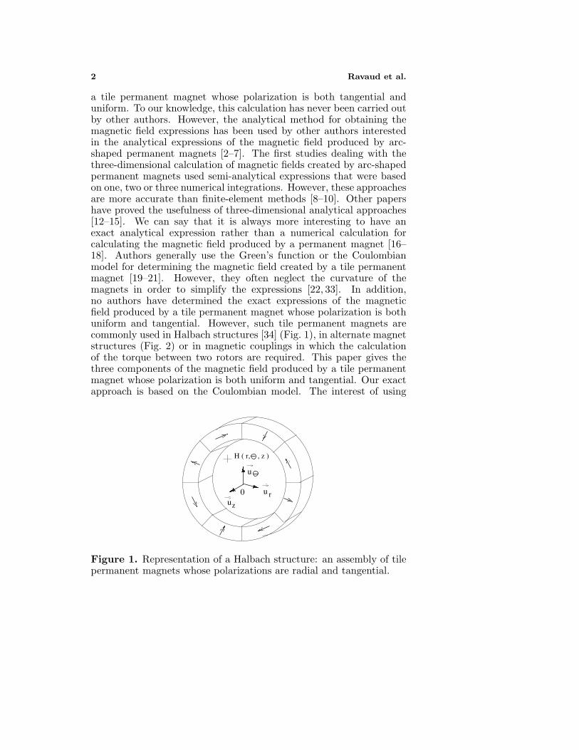
a tile permanent magnet whose polarization is both tangential anduniform. To our knowledge, this calculation has never been carried outby other authors. However, the analytical method for obtaining themagnetic field expressions has been used by other authors interestedin the analytical expressions of the magnetic field produced by arc-shaped permanent magnets [2–7]. The first studies dealing with thethree-dimensional calculation of magnetic fields created by arc-shapedpermanent magnets used semi-analytical expressions that were basedon one, two or three numerical integrations. However, these approachesare more accurate than finite-element methods [8–10]. Other papershave proved the usefulness of three-dimensional analytical approaches[12–15]. We can say that it is always more interesting to have anexact analytical expression rather than a numerical calculation forcalculating the magnetic field produced by a permanent magnet [16–18]. Authors generally use the Green’s function or the Coulombianmodel for determining the magnetic field created by a tile permanentmagnet [19–21]. However, they often neglect the curvature of themagnets in order to simplify the expressions [22, 33]. In addition,no authors have determined the exact expressions of the magneticfield produced by a tile permanent magnet whose polarization is bothuniform and tangential. However, such tile permanent magnets arecommonly used in Halbach structures [34] (Fig. 1), in alternate magnetstructures (Fig. 2) or in magnetic couplings in which the calculationof the torque between two rotors are required. This paper gives thethree components of the magnetic field produced by a tile permanentmagnet whose polarization is both uniform and tangential. Our exactapproach is based on the Coulombian model. The interest of using

H ( r, , z )

0 u ruz

u

Figure 1. Representation of a Halbach structure: an assembly of tilepermanent magnets whose polarizations are radial and tangential.

Progress In Electromagnetics Research B, Vol. 13, 2009 3

H ( r, , z )

0 u ruz

u

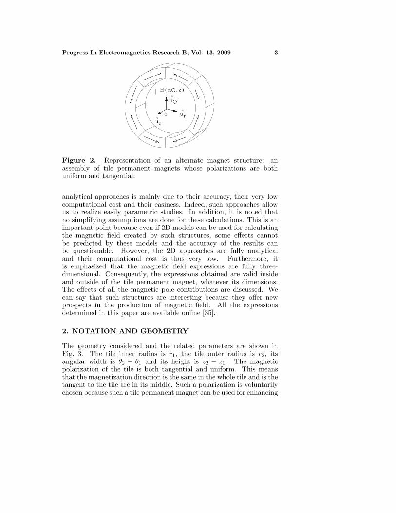
Figure 2. Representation of an alternate magnet structure: anassembly of tile permanent magnets whose polarizations are bothuniform and tangential.

analytical approaches is mainly due to their accuracy, their very lowcomputational cost and their easiness. Indeed, such approaches allowus to realize easily parametric studies. In addition, it is noted thatno simplifying assumptions are done for these calculations. This is animportant point because even if 2D models can be used for calculatingthe magnetic field created by such structures, some effects cannotbe predicted by these models and the accuracy of the results canbe questionable. However, the 2D approaches are fully analyticaland their computational cost is thus very low. Furthermore, itis emphasized that the magnetic field expressions are fully three-dimensional. Consequently, the expressions obtained are valid insideand outside of the tile permanent magnet, whatever its dimensions.The effects of all the magnetic pole contributions are discussed. Wecan say that such structures are interesting because they offer newprospects in the production of magnetic field. All the expressionsdetermined in this paper are available online [35].

2. NOTATION AND GEOMETRY

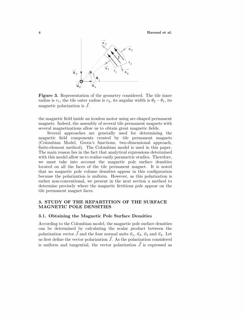
The geometry considered and the related parameters are shown inFig. 3. The tile inner radius is r1, the tile outer radius is r2, itsangular width is θ2 − θ1 and its height is z2 − z1. The magneticpolarization of the tile is both tangential and uniform. This meansthat the magnetization direction is the same in the whole tile and is thetangent to the tile arc in its middle. Such a polarization is voluntarilychosen because such a tile permanent magnet can be used for enhancing

4 Ravaud et al.

J

u

u

n

n

n

2

3

4

1n

1

2

r

r1

2

uz x

y

Figure 3. Representation of the geometry considered. The tile innerradius is r1, the tile outer radius is r2, its angular width is θ2 − θ1, itsmagnetic polarization is �J .

the magnetic field inside an ironless motor using arc-shaped permanentmagnets. Indeed, the assembly of several tile permanent magnets withseveral magnetizations allow us to obtain great magnetic fields.

Several approaches are generally used for determining themagnetic field components created by tile permanent magnets(Colombian Model, Green’s functions, two-dimensional approach,finite-element method). The Colombian model is used in this paper.The main reason lies in the fact that analytical expressions determinedwith this model allow us to realize easily parametric studies. Therefore,we must take into account the magnetic pole surface densitieslocated on all the faces of the tile permanent magnet. It is notedthat no magnetic pole volume densities appear in this configurationbecause the polarization is uniform. However, as this polarization israther non-conventional, we present in the next section a method todetermine precisely where the magnetic fictitious pole appear on thetile permanent magnet faces.

3. STUDY OF THE REPARTITION OF THE SURFACEMAGNETIC POLE DENSITIES

3.1. Obtaining the Magnetic Pole Surface Densities

According to the Colombian model, the magnetic pole surface densitiescan be determined by calculating the scalar product between thepolarization vector �J and the four normal units �n1, �n2, �n3 and �n4. Letus first define the vector polarization �J . As the polarization consideredis uniform and tangential, the vector polarization �J is expressed as


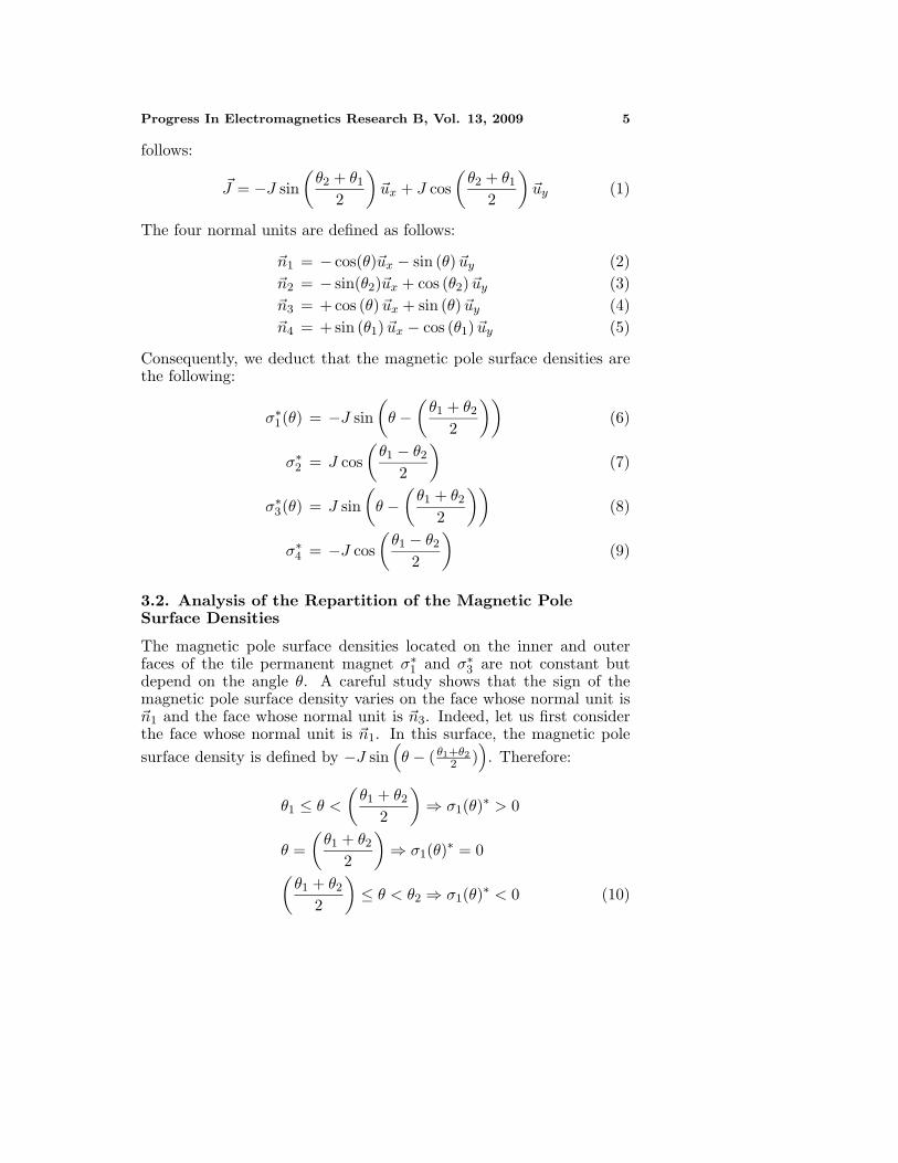
follows:

�J = −J sin(

θ2 + θ1

2

)�ux + J cos

(θ2 + θ1

2

)�uy (1)

The four normal units are defined as follows:

�n1 = − cos(θ)�ux − sin (θ) �uy (2)�n2 = − sin(θ2)�ux + cos (θ2) �uy (3)�n3 = + cos (θ) �ux + sin (θ) �uy (4)�n4 = + sin (θ1) �ux − cos (θ1) �uy (5)

Consequently, we deduct that the magnetic pole surface densities arethe following:

σ∗1(θ) = −J sin

(θ −

(θ1 + θ2

2

))(6)

σ∗2 = J cos

(θ1 − θ2

2

)(7)

σ∗3(θ) = J sin

(θ −

(θ1 + θ2

2

))(8)

σ∗4 = −J cos

(θ1 − θ2

2

)(9)

3.2. Analysis of the Repartition of the Magnetic PoleSurface Densities

The magnetic pole surface densities located on the inner and outerfaces of the tile permanent magnet σ∗

1 and σ∗3 are not constant but

depend on the angle θ. A careful study shows that the sign of themagnetic pole surface density varies on the face whose normal unit is�n1 and the face whose normal unit is �n3. Indeed, let us first considerthe face whose normal unit is �n1. In this surface, the magnetic polesurface density is defined by −J sin

(θ − ( θ1+θ2

2 )). Therefore:

θ1 ≤ θ <

(θ1 + θ2

2

)⇒ σ1(θ)∗ > 0

θ =(

θ1 + θ2

2

)⇒ σ1(θ)∗ = 0

(θ1 + θ2

2

)≤ θ < θ2 ⇒ σ1(θ)∗ < 0 (10)

6 Ravaud et al.

Let us now consider the face whose normal unit is �n3 in which themagnetic pole surface density is defined by J sin

(θ − ( θ1+θ2

2 )). We

deduct the following relations:

θ1 ≤ θ <

(θ1 + θ2

2

)⇒ σ3(θ)∗ < 0

θ =(

θ1 + θ2

2

)⇒ σ3(θ)∗ = 0

(θ1 + θ2

2

)≤ θ < θ2 ⇒ σ3(θ)∗ > 0 (11)

Let us now consider the face whose normal unit is �n2 in which themagnetic pole surface density is defined by J cos

(θ1−θ2

2

). We call this

face f2. We deduct directly that

∀θ ∈ f2 ⇒ σ∗2 > 0 (12)

By the same token, for the face whose normal unit is �n4 in whichthe magnetic pole surface density is defined by −J cos

(θ1−θ2

2

)and by

using the notation f4 for this face, we deduct that:

∀θ ∈ f4 ⇒ σ∗4 < 0 (13)

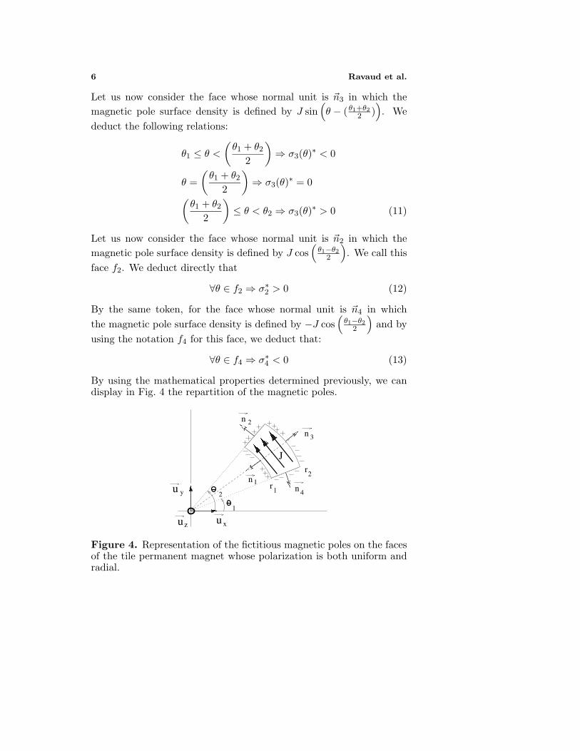
By using the mathematical properties determined previously, we candisplay in Fig. 4 the repartition of the magnetic poles.

J

u

n

n

n

2

3

4

1n

1

2

r

r1

2

uz

u

x

y

Figure 4. Representation of the fictitious magnetic poles on the facesof the tile permanent magnet whose polarization is both uniform andradial.


4. EXPRESSION OF THE THREE COMPONENTS Hr,Hθ, Hz

These three components are functions of the parameters r, θ and z.

4.1. Basic Equation

The magnetic field created by a tile permanent magnet whosepolarization is both uniform and tangential can be determined by usingthe Coulombian model. By definition, the magnetic field H(r, θ, z)created by this magnet is expressed as follows:

H(r, θ, z) =∫ ∫

S1

σ1(θ)∗

4πµ0

�u1

| �u1|3dS1

+∫ ∫

S2

σ∗2

4πµ0

�u2

| �u2|3dS2

+∫ ∫

S3

σ3(θ)∗

4πµ0

�u3

| �u3|3dS3

+∫ ∫

S4

σ∗4

4πµ0

�u4

| �u4|3dS4 (14)

where �ui is the vector between the observation point and a point owingto the surface Si.

It is noted that �u1, �u2, �u3 and �u4 are expressed in a generalform because we are interested in a three-dimensional solution forcalculating the magnetic field for all points in space. The integrationof (14) leads to the three magnetic field components along the threedefined axes: Hr(r, θ, z), Hθ(r, θ, z) and Hz(r, θ, z).

4.2. Radial Component

The radial component of the magnetic field created by a tile permanentmagnet whose polarization is both uniform and tangential can beexpressed as follows:

Hr(r, θ, z) =2∑

i=1

2∑j=1

(−1)(i+j)h(I)r (ri, zj)

+2∑

i=1

2∑j=1

2∑k=1

(−1)(i+j+k)h(II)r (ri, zj , θk) (15)

8 Ravaud et al.

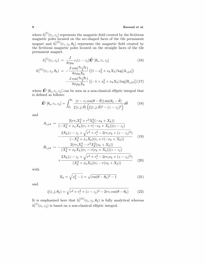
where h(I)r (ri, zj) represents the magnetic field created by the fictitious

magnetic poles located on the arc-shaped faces of the tile permanentmagnet and h

(II)r (ri, zj , θk) represents the magnetic field created by

the fictitious magnetic poles located on the straight faces of the tilepermanent magnet.

h(I)r (ri, zj) =

J

4πµ0ri(z − zj)E∗ [θa, ri, zj ] (16)

h(II)r (ri, zj , θk) = −J cos( θ1−θ2

2 )8πµ0Xk

((1 − x2

k + xkXk) log[Ai,j,k])

−J cos( θ1−θ22 )

8πµ0Xk

((−1 + x2

k + xkXk) log[Bi,j,k])(17)

where E∗ [θa, ri, zj ] can be seen as a non-classical elliptic integral thatis defined as follows:

E∗ [θa, ri, zj ] =∫ θ2

θ1

(r − ri cos(θ − θ)) sin(θa − θ)

ξ(i, j, θ)(ξ(i, j, θ)2 − (z − zj)2

)dθ (18)

and

Ai,j,k =2(rriX

2k + r2X2

k(−xk + Xk))(−X2

k + xxXk)(ri + r(−xk + Xk))(z − zj)

−2Xk(z − zj +

√r2 + r2

i − 2rrixk + (z − zj)2)

(−X2k + xxXk)(ri + r(−xk + Xk))

(19)

Bi,j,k = − 2(rriX2k − r2X2

k(xk + Xk))(X2

k + xkXk)(ri − r(xk + Xk))(z − zj)

+2Xk(z − zj +

√r2 + r2

i − 2rrixk + (z − zj)2)

(X2k + xkXk)(ri − r(xk + Xk))

(20)

with

Xk =√

x2k − 1 =

√cos(θ − θk)2 − 1 (21)

and

ξ(i, j, θk) =√

r2 + r2i + (z − zj)2 − 2rri cos(θ − θk) (22)

It is emphasized here that h(II)r (ri, zj , θk) is fully analytical whereas

h(I)r (ri, zj) is based on a non-classical elliptic integral.


It has to be noted that all the numerical calculations to illustratethe analytical formulations will be done in this section for the followingtile dimensions: r1 = 0.025 m, r2 = 0.028 m, z2 − z1 = 0.003 m,θ2 − θ1 = π

6 rad. Moreover, the polarization is J = 1 T and theobservation path always corresponds to: z = 0.001 m, r = 0.024 m.

Figure 5 represents the radial component versus the angle θ forthe defined set of values.

3 2 1 0 1 2 3Angle [rad]

75000

50000

25000

0

25000

50000

75000

Hr

[A/m

]

−

−

−

− − −

Figure 5. Representation of the radial component Hr of the magneticfield created by a tile permanent magnet whose polarization is bothuniform and tangential. We take r1 = 0.025 m, r2 = 0.028 m, itsangular width is θ2 − θ1 = π

6 rad, J = 1 T, z = 0.001 m, r = 0.024 m,z2 − z1 = 0.003 m.

4.3. Azimuthal Component

The azimuthal component of the magnetic field created by a tilepermanent magnet whose polarization is both uniform and tangentialis expressed as follows:

Hθ(r, θ, z) =2∑

i=1

2∑j=1

(−1)(i+j)h(I)θ (ri, zj)

+2∑

i=1

2∑j=1

2∑k=1

(−1)(1+i+j+k)h(II)θ (ri, zj , θk) (23)

with

h(I)θ (ri, zj) =

J

4πµ0r2i (zj − z)L∗

[θ1 + θ2

2, ri, zj

](24)

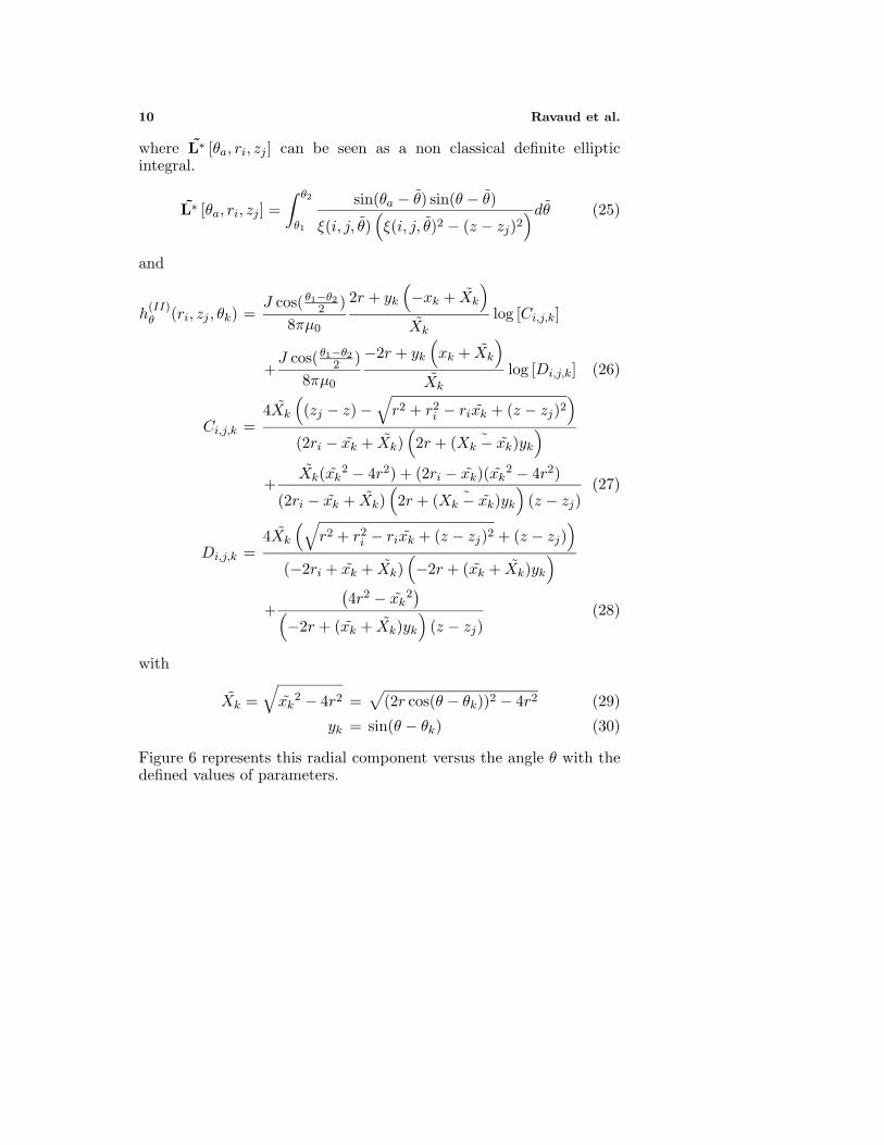
10 Ravaud et al.

where L∗ [θa, ri, zj ] can be seen as a non classical definite ellipticintegral.

L∗ [θa, ri, zj ] =∫ θ2

θ1

sin(θa − θ) sin(θ − θ)

ξ(i, j, θ)(ξ(i, j, θ)2 − (z − zj)2

)dθ (25)

and

h(II)θ (ri, zj , θk) =

J cos( θ1−θ22 )

8πµ0

2r + yk

(−xk + Xk

)Xk

log [Ci,j,k]

+J cos( θ1−θ2

2 )8πµ0

−2r + yk

(xk + Xk

)Xk

log [Di,j,k] (26)

Ci,j,k =4Xk

((zj − z) −

√r2 + r2

i − rixk + (z − zj)2)

(2ri − xk + Xk)(2r + ( ˜Xk − xk)yk

)

+Xk(xk

2 − 4r2) + (2ri − xk)(xk2 − 4r2)

(2ri − xk + Xk)(2r + ( ˜Xk − xk)yk

)(z − zj)

(27)

Di,j,k =4Xk

(√r2 + r2

i − rixk + (z − zj)2 + (z − zj))

(−2ri + xk + Xk)(−2r + (xk + Xk)yk

)

+

(4r2 − xk

2)

(−2r + (xk + Xk)yk

)(z − zj)

(28)

with

Xk =√

xk2 − 4r2 =

√(2r cos(θ − θk))2 − 4r2 (29)

yk = sin(θ − θk) (30)

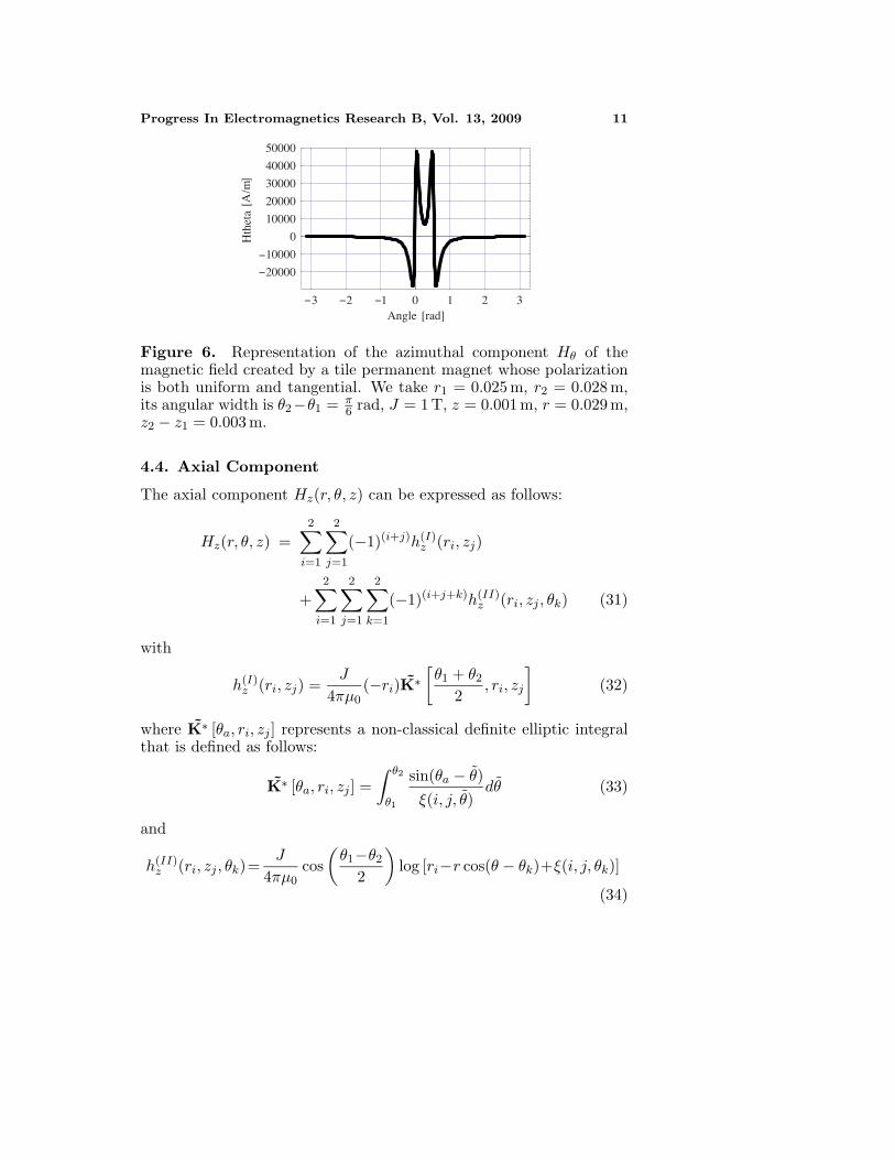
Figure 6 represents this radial component versus the angle θ with thedefined values of parameters.


3 2 1 0 1 2 3Angle [rad]

20000

10000

0

10000

20000

30000

40000

50000

Hth

eta

−−

− − −

[A/m

]

Figure 6. Representation of the azimuthal component Hθ of themagnetic field created by a tile permanent magnet whose polarizationis both uniform and tangential. We take r1 = 0.025 m, r2 = 0.028 m,its angular width is θ2−θ1 = π

6 rad, J = 1 T, z = 0.001 m, r = 0.029 m,z2 − z1 = 0.003 m.

4.4. Axial Component

The axial component Hz(r, θ, z) can be expressed as follows:

Hz(r, θ, z) =2∑

i=1

2∑j=1

(−1)(i+j)h(I)z (ri, zj)

+2∑

i=1

2∑j=1

2∑k=1

(−1)(i+j+k)h(II)z (ri, zj , θk) (31)

with

h(I)z (ri, zj) =

J

4πµ0(−ri)K∗

[θ1 + θ2

2, ri, zj

](32)

where K∗ [θa, ri, zj ] represents a non-classical definite elliptic integralthat is defined as follows:

K∗ [θa, ri, zj ] =∫ θ2

θ1

sin(θa − θ)ξ(i, j, θ)

dθ (33)

and

h(II)z (ri, zj , θk)=

J

4πµ0cos

(θ1−θ2

2

)log [ri−r cos(θ − θk)+ξ(i, j, θk)]

(34)

12 Ravaud et al.

3 2 1 0 1 2 3Angle [rad]

10000

5000

0

5000

10000

Hz

−

−

− − −

[A/m

]

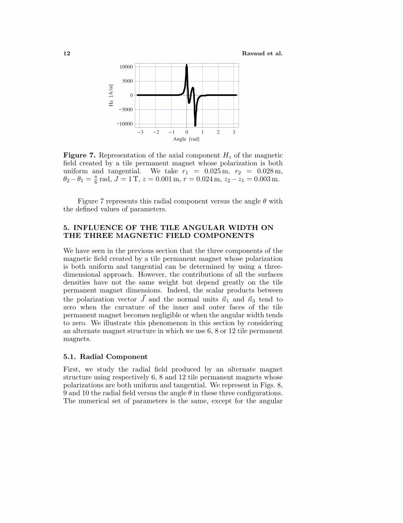
Figure 7. Representation of the axial component Hz of the magneticfield created by a tile permanent magnet whose polarization is bothuniform and tangential. We take r1 = 0.025 m, r2 = 0.028 m,θ2−θ1 = π

6 rad, J = 1 T, z = 0.001 m, r = 0.024 m, z2−z1 = 0.003 m.

Figure 7 represents this radial component versus the angle θ withthe defined values of parameters.

5. INFLUENCE OF THE TILE ANGULAR WIDTH ONTHE THREE MAGNETIC FIELD COMPONENTS

We have seen in the previous section that the three components of themagnetic field created by a tile permanent magnet whose polarizationis both uniform and tangential can be determined by using a three-dimensional approach. However, the contributions of all the surfacesdensities have not the same weight but depend greatly on the tilepermanent magnet dimensions. Indeed, the scalar products betweenthe polarization vector �J and the normal units �n1 and �n3 tend tozero when the curvature of the inner and outer faces of the tilepermanent magnet becomes negligible or when the angular width tendsto zero. We illustrate this phenomenon in this section by consideringan alternate magnet structure in which we use 6, 8 or 12 tile permanentmagnets.

5.1. Radial Component

First, we study the radial field produced by an alternate magnetstructure using respectively 6, 8 and 12 tile permanent magnets whosepolarizations are both uniform and tangential. We represent in Figs. 8,9 and 10 the radial field versus the angle θ in these three configurations.The numerical set of parameters is the same, except for the angular


−

−

0 1 2 3 4 5 6Angle [rad]

100000

50000

0

50000

100000

Hth

eta

[A/m

]

Figure 8. Representation of the radial component Hr of the magneticfield created by an alternate magnet structure owing 6 tile permanentmagnets whose polarization is both uniform and tangential. We taker1 = 0.025 m, r2 = 0.028 m, θ2 − θ1 = π

3 rad, J = 1 T, z = 0.001 m,r = 0.024 m, z2 − z1 = 0.003 m.

0 1 2 3 4 5 6Angle [rad]

100000

50000

0

50000

100000

Hth

eta

[A/m

]

−

−

Figure 9. Representation of the radial component Hr of the magneticfield created by an alternate magnet structure owing 8 tile permanentmagnets whose polarization is both uniform and tangential. We taker1 = 0.025 m, r2 = 0.028 m, θ2 − θ1 = π

4 rad, J = 1 T, z = 0.001 m,r = 0.024 m, z2 − z1 = 0.003 m.

width which depends on the tile number and will be specified in eachcase. Figs. 8, 9 and 10 clearly show that the effects of the magneticpole surface densities located on the inner and outer faces of thetile permanent magnet become negligible when the angular width ofthe tile permanent magnet decreases. This is in fact an interestingpoint because it gives indications about the number of tile permanentmagnets that should be used in ironless structures. Indeed, if a greatradial field is required, it is more interesting to use 12 tiles rather than 6

14 Ravaud et al.

0 1 2 3 4 5 6Angle [rad]

150000

100000

50000

0

50000

100000

150000

Hth

eta

[A/m

]−

−

−

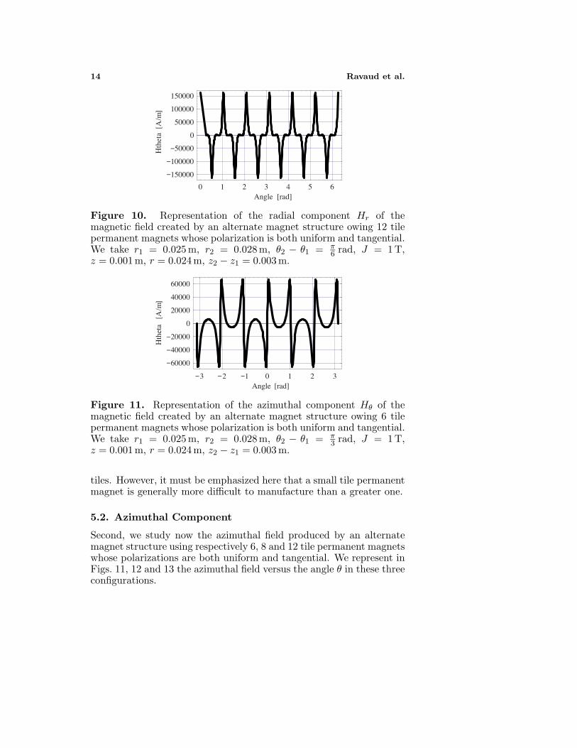
Figure 10. Representation of the radial component Hr of themagnetic field created by an alternate magnet structure owing 12 tilepermanent magnets whose polarization is both uniform and tangential.We take r1 = 0.025 m, r2 = 0.028 m, θ2 − θ1 = π

6 rad, J = 1 T,z = 0.001 m, r = 0.024 m, z2 − z1 = 0.003 m.

3 2 1 0 1 2 3Angle [rad]

60000

40000

20000

0

20000

40000

60000

Hth

eta

[A/m

]

−

−

−

− − −

Figure 11. Representation of the azimuthal component Hθ of themagnetic field created by an alternate magnet structure owing 6 tilepermanent magnets whose polarization is both uniform and tangential.We take r1 = 0.025 m, r2 = 0.028 m, θ2 − θ1 = π

3 rad, J = 1 T,z = 0.001 m, r = 0.024 m, z2 − z1 = 0.003 m.

tiles. However, it must be emphasized here that a small tile permanentmagnet is generally more difficult to manufacture than a greater one.

5.2. Azimuthal Component

Second, we study now the azimuthal field produced by an alternatemagnet structure using respectively 6, 8 and 12 tile permanent magnetswhose polarizations are both uniform and tangential. We represent inFigs. 11, 12 and 13 the azimuthal field versus the angle θ in these threeconfigurations.


3 2 1 0 1 2 3Angle [rad]

60000

40000

20000

0

20000

40000

60000

Hth

eta

−

−

−

− − −

[A/m

]

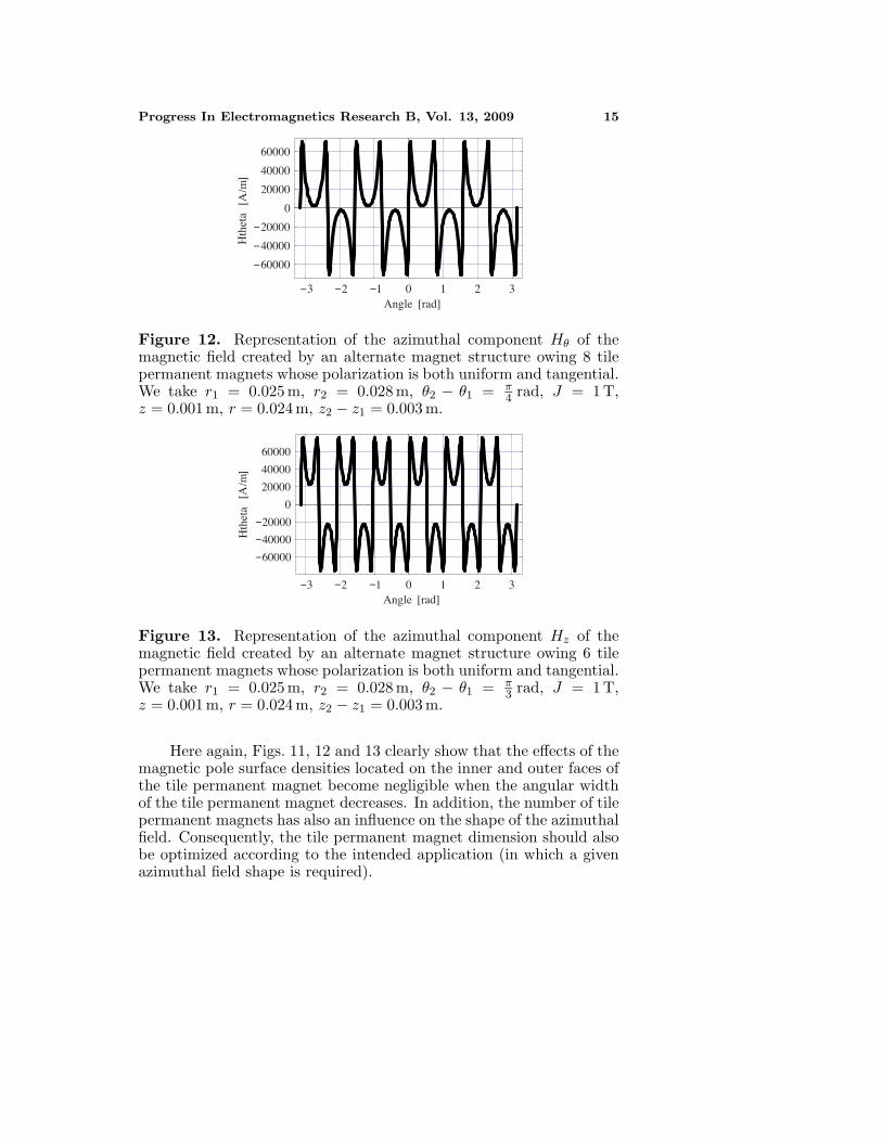
Figure 12. Representation of the azimuthal component Hθ of themagnetic field created by an alternate magnet structure owing 8 tilepermanent magnets whose polarization is both uniform and tangential.We take r1 = 0.025 m, r2 = 0.028 m, θ2 − θ1 = π

4 rad, J = 1 T,z = 0.001 m, r = 0.024 m, z2 − z1 = 0.003 m.

3 2 1 0 1 2 3Angle [rad]

60000

40000

20000

0

20000

40000

60000

Hth

eta

[A/m

]

−

−

−

− − −

Figure 13. Representation of the azimuthal component Hz of themagnetic field created by an alternate magnet structure owing 6 tilepermanent magnets whose polarization is both uniform and tangential.We take r1 = 0.025 m, r2 = 0.028 m, θ2 − θ1 = π

3 rad, J = 1 T,z = 0.001 m, r = 0.024 m, z2 − z1 = 0.003 m.

Here again, Figs. 11, 12 and 13 clearly show that the effects of themagnetic pole surface densities located on the inner and outer faces ofthe tile permanent magnet become negligible when the angular widthof the tile permanent magnet decreases. In addition, the number of tilepermanent magnets has also an influence on the shape of the azimuthalfield. Consequently, the tile permanent magnet dimension should alsobe optimized according to the intended application (in which a givenazimuthal field shape is required).

16 Ravaud et al.

[A/m

]

0 1 2 3 4 5 6Angle [rad]

30000

20000

10000

0

10000

20000

30000

Hz

−

−

−

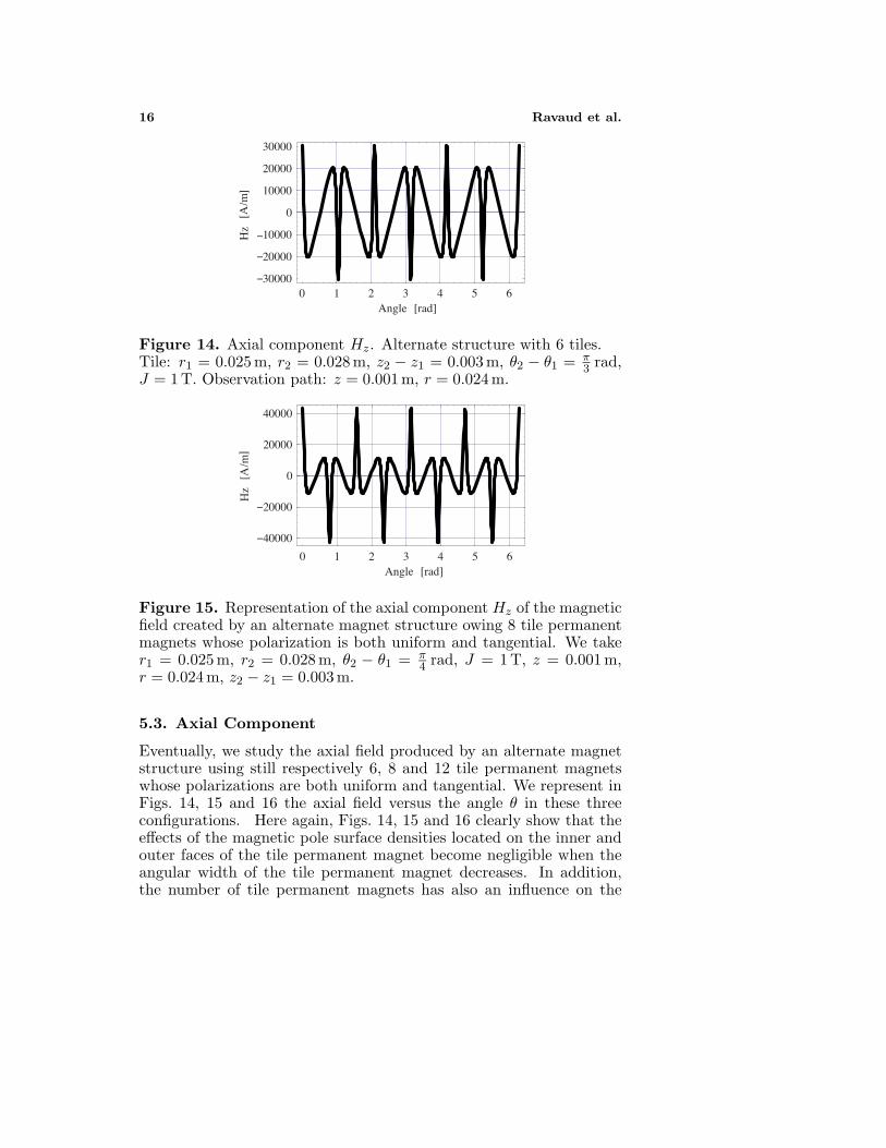
Figure 14. Axial component Hz. Alternate structure with 6 tiles.Tile: r1 = 0.025 m, r2 = 0.028 m, z2 − z1 = 0.003 m, θ2 − θ1 = π

3 rad,J = 1 T. Observation path: z = 0.001 m, r = 0.024 m.

0 1 2 3 4 5 6Angle [rad]

40000

20000

0

20000

40000

Hz

[A/m

]

−

−

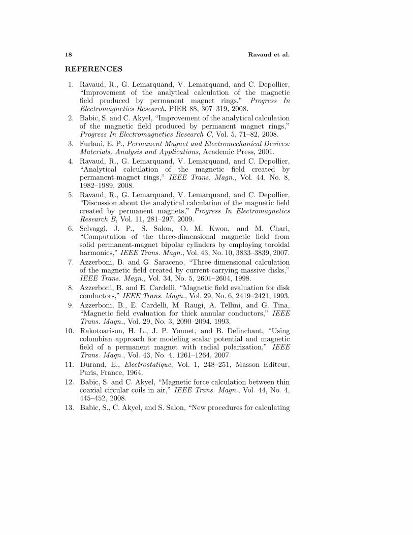
Figure 15. Representation of the axial component Hz of the magneticfield created by an alternate magnet structure owing 8 tile permanentmagnets whose polarization is both uniform and tangential. We taker1 = 0.025 m, r2 = 0.028 m, θ2 − θ1 = π

4 rad, J = 1 T, z = 0.001 m,r = 0.024 m, z2 − z1 = 0.003 m.

5.3. Axial Component

Eventually, we study the axial field produced by an alternate magnetstructure using still respectively 6, 8 and 12 tile permanent magnetswhose polarizations are both uniform and tangential. We represent inFigs. 14, 15 and 16 the axial field versus the angle θ in these threeconfigurations. Here again, Figs. 14, 15 and 16 clearly show that theeffects of the magnetic pole surface densities located on the inner andouter faces of the tile permanent magnet become negligible when theangular width of the tile permanent magnet decreases. In addition,the number of tile permanent magnets has also an influence on the


0 1 2 3 4 5 6Angle [rad]

40000

20000

0

20000

40000

Hz

[A/m

]−

−

Figure 16. Representation of the axial component Hz of the magneticfield created by an alternate magnet structure owing 12 tile permanentmagnets whose polarization is both uniform and tangential. We taker1 = 0.025 m, r2 = 0.028 m, θ2 − θ1 = π

6 rad, J = 1 T, z = 0.001 m,r = 0.024 m, z2 − z1 = 0.003 m.

shape of the axial field. For example, Fig. 14 shows that the use ofonly 6 permanent magnets in an ironless structure whose diameteris small (here 0.05 m) is not sufficient. Thus, our three-dimensionalapproach allows us to optimize easily magnet dimensions for studyingthe magnetic field produced by such structures.

6. CONCLUSION

This paper has presented 3D analytical expressions for studying themagnetic field created by a tile permanent magnet whose polarizationis both uniform and tangential. The three magnetic components of thismagnetic field are determined by using the Colombian model. As nosimplifying assumptions are used for calculating the radial, axial andazimuthal fields created by a tile permanent magnet, our expressionsare valid for all points in space, whatever the magnet dimensions. Wealso discuss the influence of the angular width of a tile permanentmagnet on the field produced. The results obtained confirm that thescalar product �J · �ni where �ni is the normal unit of the face i can be agood indicator for studying the effects of all the magnetic pole chargecontributions on the magnetic field created. The expressions given inthis paper are available online [35] and for each expression, a numericalcalculation has been carried out for confirming our three-dimensionalapproach.

18 Ravaud et al.

REFERENCES

1. Ravaud, R., G. Lemarquand, V. Lemarquand, and C. Depollier,“Improvement of the analytical calculation of the magneticfield produced by permanent magnet rings,” Progress InElectromagnetics Research, PIER 88, 307–319, 2008.

2. Babic, S. and C. Akyel, “Improvement of the analytical calculationof the magnetic field produced by permanent magnet rings,”Progress In Electromagnetics Research C, Vol. 5, 71–82, 2008.

3. Furlani, E. P., Permanent Magnet and Electromechanical Devices:Materials, Analysis and Applications, Academic Press, 2001.

4. Ravaud, R., G. Lemarquand, V. Lemarquand, and C. Depollier,“Analytical calculation of the magnetic field created bypermanent-magnet rings,” IEEE Trans. Magn., Vol. 44, No. 8,1982–1989, 2008.

5. Ravaud, R., G. Lemarquand, V. Lemarquand, and C. Depollier,“Discussion about the analytical calculation of the magnetic fieldcreated by permanent magnets,” Progress In ElectromagneticsResearch B, Vol. 11, 281–297, 2009.

6. Selvaggi, J. P., S. Salon, O. M. Kwon, and M. Chari,“Computation of the three-dimensional magnetic field fromsolid permanent-magnet bipolar cylinders by employing toroidalharmonics,” IEEE Trans. Magn., Vol. 43, No. 10, 3833–3839, 2007.

7. Azzerboni, B. and G. Saraceno, “Three-dimensional calculationof the magnetic field created by current-carrying massive disks,”IEEE Trans. Magn., Vol. 34, No. 5, 2601–2604, 1998.

8. Azzerboni, B. and E. Cardelli, “Magnetic field evaluation for diskconductors,” IEEE Trans. Magn., Vol. 29, No. 6, 2419–2421, 1993.

9. Azzerboni, B., E. Cardelli, M. Raugi, A. Tellini, and G. Tina,“Magnetic field evaluation for thick annular conductors,” IEEETrans. Magn., Vol. 29, No. 3, 2090–2094, 1993.

10. Rakotoarison, H. L., J. P. Yonnet, and B. Delinchant, “Usingcolombian approach for modeling scalar potential and magneticfield of a permanent magnet with radial polarization,” IEEETrans. Magn., Vol. 43, No. 4, 1261–1264, 2007.

11. Durand, E., Electrostatique, Vol. 1, 248–251, Masson Editeur,Paris, France, 1964.

12. Babic, S. and C. Akyel, “Magnetic force calculation between thincoaxial circular coils in air,” IEEE Trans. Magn., Vol. 44, No. 4,445–452, 2008.

13. Babic, S., C. Akyel, and S. Salon, “New procedures for calculating


the mutual inductance of the system: Filamentary circular coil-massive circular solenoid,” IEEE Trans. Magn., Vol. 39, No. 3,1131–1134, 2003.

14. Babic, S., C. Akyel, S. Salon, and S. Kincic, “New expressions forcalculating the magnetic field created by radial current in massivedisks,” IEEE Trans. Magn., Vol. 38, No. 2, 497–500, 2002.

15. Babic, S., S. Salon, and C. Akyel, “The mutual inductance of twothin coaxial disk coils in air,” IEEE Trans. Magn., Vol. 40, No. 2,822–825, 2004.

16. Conway, J., “Noncoaxial inductance calculations without thevector potential for axisymmetric coils and planar coils,” IEEETrans. Magn., Vol. 44, No. 10, 453–462, 2008.

17. Furlani, E. P., S. Reznik, and A. Kroll, “A three-dimensional fieldsolution for radially polarized cylinders,” IEEE Trans. Magn.,Vol. 31, No. 1, 844–851, 1995.

18. Furlani, E. P., “Field analysis and optimization of NDFEB axialfield permanent magnet motors,” IEEE Trans. Magn., Vol. 33,No. 5, 3883–3885, 1997.

19. Furlani, E. P. and M. Knewston, “A three-dimensional fieldsolution for permanent-magnet axial-field motors,” IEEE Trans.Magn., Vol. 33, No. 1, 2322–2325, 1997.

20. Furlani, E. P., “A two-dimensional analysis for the coupling ofmagnetic gears,” IEEE Trans. Magn., Vol. 33, No. 3, 2317–2321,1997.

21. Mayergoyz, D. and E. P. Furlani, “The Computation ofmagnetic fields of permanent magnet cylinders used in theelectrophotographic process,” J. Appl. Phys., Vol. 73, No. 10,5440–5442, 1993.

22. Yonnet, J. P., “Passive magnetic bearings with permanentmagnets,” IEEE Trans. Magn., Vol. 14, No. 5, 803–805, 1978.

23. Abele, M., J. Jensen, and H. Rusinek, “Generation of uniformhigh fields with magnetized wedges,” IEEE Trans. Magn., Vol. 33,No. 5, 3874–3876, 1997.

24. Aydin, M., Z. Zhu, T. Lipo, and D. Howe, “Minimization ofcogging torque in axial-flux permanent-magnet machines: Designconcepts,” IEEE Trans. Magn., Vol. 43, No. 9, 3614–3622, 2007.

25. Marinescu, M. and N. Marinescu, “Compensation of anisotropyeffects in flux-confining permanent-magnet structures,” IEEETrans. Magn., Vol. 25, No. 5, 3899–3901, 1989.

26. Akoun, G. and J. P. Yonnet, “3d analytical calculation of theforces exerted between two cuboidal magnets,” IEEE Trans.

20 Ravaud et al.

Magn., Vol. 20, No. 5, 1962–1964, 1984.27. Yong, L., Z. Jibin, and L. Yongping, “Optimum design of magnet

shape in permanent-magnet synchronous motors,” IEEE Trans.Magn., Vol. 39, No. 11, 3523–4205, 2003.

28. Lemarquand, G. and V. Lemarquand, “Annular magnet positionsensor,” IEEE. Trans. Magn., Vol. 26, No. 5, 2041–2043, 1990.

29. Yonnet, J. P., “Permanent magnet bearings and couplings,” IEEETrans. Magn., Vol. 17, No. 1, 1169–1173, 1981.

30. Zhu, Z. and D. Howe, “Analytical prediction of the cogging torquein radial-field permanent magnet brushless motors,” IEEE Trans.Magn., Vol. 28, No. 2, 1371–1374, 1992.

31. Wang, J., G. W. Jewell, and D. Howe, “Design optimisation andcomparison of permanent magnet machines topologies,” IEE Proc.Elect. Power Appl., Vol. 148, 456–464, 2001.

32. Yonnet, J. P., Rare-earth Iron Permanent Magnets, Ch. Magne-tomechanical devices, Oxford Science Publications, 1996.

33. Blache, C. and G. Lemarquand, “New structures for lineardisplacement sensor with hight magnetic field gradient,” IEEETrans. Magn., Vol. 28, No. 5, 2196–2198, 1992.

34. Halbach, K., “Design of permanent multiple magnets withoriented rec material,” Nucl. Inst. Meth., Vol. 169, 1–10, 1980.

35. http://www.univ-lemans.fr/∼glemar

Magnetic Field Produced by a Tile Permanent Magnet Whose ...

Documents