REVIEW ARTICLE Magnetars: the physics behind observations R Turolla 1,2 , S Zane 2 , A L Watts 3 1 Department of Physics and Astronomy, University of Padova, via Marzolo 8, 35131 Padova, Italy 2 Mullard Space Science Laboratory, University College London, Holbury St. Mary, Surrey, RH5 6NT, UK 3 Anton Pannekoek Institute for Astronomy, University of Amsterdam, Postbus 94249, 1090 GE Amsterdam, The Netherlands E-mail: [email protected] Abstract. Magnetars are the strongest magnets in the present universe and the combination of extreme magnetic field, gravity and density makes them unique laboratories to probe current physical theories (from quantum electrodynamics to general relativity) in the strong field limit. Magnetars are observed as peculiar, burst– active X-ray pulsars, the Anomalous X-ray Pulsars (AXPs) and the Soft Gamma Repeaters (SGRs); the latter emitted also three “giant flares”, extremely powerful events during which luminosities can reach up to 10 47 erg/s for about one second. The last five years have witnessed an explosion in magnetar research which has led, among other things, to the discovery of transient, or “outbursting”, and “low-field” magnetars. Substantial progress has been made also on the theoretical side. Quite detailed models for explaining the magnetars’ persistent X-ray emission, the properties of the bursts, the flux evolution in transient sources have been developed and confronted with observations. New insight on neutron star asteroseismology has been gained through improved models of magnetar oscillations. The long-debated issue of magnetic field decay in neutron stars has been addressed, and its importance recognized in relation to the evolution of magnetars and to the links among magnetars and other families of isolated neutron stars. The aim of this paper is to present a comprehensive overview in which the observational results are discussed in the light of the most up-to-date theoretical models and their implications. This addresses not only the particular case of magnetar sources, but the more fundamental issue of how physics in strong magnetic fields can be constrained by the observations of these unique sources. arXiv:1507.02924v1 [astro-ph.HE] 10 Jul 2015

Welcome message from author
This document is posted to help you gain knowledge. Please leave a comment to let me know what you think about it! Share it to your friends and learn new things together.
Transcript

REVIEW ARTICLE
Magnetars: the physics behind observations
R Turolla1,2, S Zane2, A L Watts3
1 Department of Physics and Astronomy, University of Padova, via Marzolo 8, 35131
Padova, Italy2 Mullard Space Science Laboratory, University College London, Holbury St. Mary,
Surrey, RH5 6NT, UK3 Anton Pannekoek Institute for Astronomy, University of Amsterdam, Postbus
94249, 1090 GE Amsterdam, The Netherlands
E-mail: [email protected]
Abstract. Magnetars are the strongest magnets in the present universe and the
combination of extreme magnetic field, gravity and density makes them unique
laboratories to probe current physical theories (from quantum electrodynamics to
general relativity) in the strong field limit. Magnetars are observed as peculiar, burst–
active X-ray pulsars, the Anomalous X-ray Pulsars (AXPs) and the Soft Gamma
Repeaters (SGRs); the latter emitted also three “giant flares”, extremely powerful
events during which luminosities can reach up to 1047 erg/s for about one second. The
last five years have witnessed an explosion in magnetar research which has led, among
other things, to the discovery of transient, or “outbursting”, and “low-field” magnetars.
Substantial progress has been made also on the theoretical side. Quite detailed
models for explaining the magnetars’ persistent X-ray emission, the properties of the
bursts, the flux evolution in transient sources have been developed and confronted with
observations. New insight on neutron star asteroseismology has been gained through
improved models of magnetar oscillations. The long-debated issue of magnetic field
decay in neutron stars has been addressed, and its importance recognized in relation
to the evolution of magnetars and to the links among magnetars and other families of
isolated neutron stars. The aim of this paper is to present a comprehensive overview
in which the observational results are discussed in the light of the most up-to-date
theoretical models and their implications. This addresses not only the particular case
of magnetar sources, but the more fundamental issue of how physics in strong magnetic
fields can be constrained by the observations of these unique sources.arX
iv:1
507.
0292
4v1
[as
tro-
ph.H
E]
10
Jul 2
015

Magnetars: the physics behind observations 2
1. Introduction
Neutron stars (NSs), the endpoint of the evolution of massive stars with 10 .M/M� .25, are extremely compact remnants endowed with strong magnetic fields. Isolated (i.e.
not belonging to a binary system) neutron stars were for a long time identified with radio-
pulsars, and only in the last two decades, mainly thanks to high-energy observations,
was the existence of other manifestations of isolated neutron stars recognized. Among
them, there are two groups of X-ray pulsars with remarkably peculiar properties, the
Soft Gamma Repeaters (SGRs) and the Anomalous X-ray Pulsars (AXPs, see e.g.
Mereghetti, 2008, for a review). The separation into two classes reflects the way in which
these sources were originally discovered. SGRs were revealed through the detection of
short, intense bursts in the hard X-/soft gamma-ray range (Mazets et al., 1979b,a), and
because of this were initially associated with gamma ray bursts (GRBs); however, burst
emission from SGRs was soon recognized to repeat, at variance to what was observed in
GRBs, setting the two phenomena apart. On the other hand, AXPs were identified as
X-ray pulsar in the soft X-ray range (< 10 keV, Mereghetti & Stella, 1995). They were
dubbed “anomalous” because their high X-ray luminosity (∼ 1034 − 1036 erg/s) cannot
be easily explained in terms of the conventional processes which apply to other classes of
pulsars, i.e. accretion from a binary companion or injection of rotational energy in the
pulsar wind/magnetosphere. Over the last few years, observations have revealed many
similarities between these two classes of objects (see e.g. Woods & Thompson, 2006),
including the discovery that AXPs too emit short, SGR-like bursts (Kaspi, 2000, 2003)
and nowadays the idea that SGRs and AXPs belong to a single, unified class is widely
accepted.
The main observational characteristics of SGRs and AXPs are: a) lack of evidence
of binary companions; b) persistent (i.e. non-bursting), often variable X-ray luminosity
in the range ∼ 1033–1036 erg/s, emitted in the soft (0.5–10 keV) and hard (20–100 keV)
X-ray range; c) pulsations at relatively long spin periods, clustered in the range ∼ 2–12 s;
d) large secular spin-down rate, P ∼ 10−13 − 10−11 s/s, which, if interpreted in terms
of electromagnetic losses from a rotating dipole in vacuo, leads to huge magnetic fields,
∼ 1014–1015 G. SGRs (and AXPs, to a somewhat lesser extent) exhibit spectacular and
frequent bursting activity, which is observed in the X-/gamma-rays on several timescales,
ranging from sub-s to several tens of seconds. In particular, three different kinds of
bursting events have been observed (see Sec. 5):
• short bursts: these are the most common, with typical duration of ∼ 0.1–1 s, peak
luminosity of ∼ 1039–1041 erg/s, and soft (∼ 10 keV), thermal spectra; they are
detected from both SGRs and AXPs;
• intermediate bursts, which last ∼ 1–40 s and have a peak luminosity of ∼1041 − 1043 erg/s. These are characterized by an abrupt onset and usually also
show thermal spectra; again, they were seen in both SGRs and AXPs;
• giant flares. These are exceptional, rare events, with an energy output of ∼1044 − 1047 erg/s, only exceeded by blazars and GRBs. They have been observed

Magnetars: the physics behind observations 3
only in SGRs and only three times since SGRs were discovered: from SGR 0526-66
in 1979 (Mazets et al., 1979a), from SGR 1900+14 in 1998 (Hurley et al., 1999),
and from SGR 1806-20 in 2004 (e.g. Hurley et al., 2005; Palmer et al., 2005). All
three events started with an initial spike of ∼ 0.1–0.2 s duration, followed by a long
pulsating tail (lasting a few hundred seconds) modulated at the neutron star spin
period.
All together, these properties find an explanation in the so-called “magnetar”
scenario (Duncan & Thompson, 1992; Thompson & Duncan, 1993, 1995), according
to which the relatively high X-ray luminosity and the bursting/outbursting activity are
powered by the dissipation and decay of a superstrong magnetic field, ≈ 1014–1015 G on
the surface and possibly higher in the star’s interior. Despite no indisputable measure
of an ultra-high magnetic field has been obtained as yet, a number of indipendent
arguments strongly support the idea that SGRs/AXPs are indeed magnetically-powered,
as first discussed by Thompson & Duncan (1995). A few of them are
• the rotational energy loss rate E (which is believed to fuel standard pulsars) is well
below the persistent X-ray luminosity, E � LX ;
• long spin periods (≈ 10 s) can be attained in ≈ 103 − 104 yrs (the source age as
inferred from that of the associated SNR) via magneto-dipolar braking only for
fields & 1014 G;
• huge spin-down rates have been indeed measured in these sources, implying dipole
magnetic fields in the range ≈ 1014 − 1015 G;
• the decrease of the scattering opacity in a superstrong magnetic field (B & 1014
G) pushes upwards the Eddington limit and allows a much larger luminosity to
escape from a (magnetically) confined plasma: this can explain the apparently
super-Eddington luminosity of a number of bursts;
• no stellar companions have been discovered in SGRs/AXPs, ruling out accretion as
a possible source of energy;
• if no more than a fraction of the magnetic energy was released in a giant flare, this
requires B & 1014 G; in order to power ≈ 100 giant flares like that emitted in 2004
by SGR 1806-20 over the source lifetime an internal field ≈ 1016 G is needed (Stella
et al., 2005).
Although alternative interpretations have been proposed (see e.g. Turolla & Esposito,
2013, for a review and references therein), the magnetar model more naturally explains
the properties of SGRs and AXPs, including the bursting activity and the hyper-
energetic giant flares, and will be the focus of this review.
Even the “persistent” emission of these sources is far from being steady. Magnetars’
spin-down is quite irregular, and often accompanied by glitches and timing noise. Long
term variations in magnetars’ emission can occur either as gradual and moderate changes
in the flux, accompanied by variations in the spectrum, pulse profile, and spin-down rate,
or as sudden outbursts, i.e. events during which the flux raises up to a factor ∼ 1000
Magnetars: the physics behind observations 4
and then decays back to a level compatible with the quiescent state over a time scale
of months/years (see Sec. 4). Within the magnetar scenario, the first kind of variability
is thought to be driven by plastic deformations in the crust which, in turn, induce
changes in the magnetic current configurations. The more violent outbursts, as well as
the glitches, the bursting activity and even the hyper-energetic giant flares could instead
be due to sudden reconfigurations of the magnetosphere, when unstable conditions are
reached. This may lead to crustal fractures (starquakes) and/or instabilities in the outer
magnetosphere (possibly involving magnetic reconnection).
Although originally discovered in the X-/soft gamma-rays, magnetars have
been detected at different wavelengths, revealing a rich phenomenology across the
electromagnetic spectrum. AXPs and SGRs have been discovered to emit in the optical
and/or near-infrared (NIR) bands (e.g. Hulleman et al., 2000; Israel et al., 2004; Durant
& van Kerkwijk, 2006). The optical/NIR counterparts are faint (K ∼ 20) and the flux
is only a small fraction of the bolometric flux, but still its detection can place important
constraints on models. Several AXPs have exhibited long-term variability both in their
optical/infrared emission and in X-rays (Israel et al., 2002; Hulleman et al., 2004; Rea
et al., 2005). Unavoidably this introduces additional uncertainties in the modelling of
broad band spectra, based on observations at different wavelengths taken at different
times.
Magnetars were traditionally considered to be radio-silent, but this picture was
challenged by the (unexpected) discovery of a pulsed radio counterpart in some sources,
a property that seems to be peculiar to transient magnetars (Gelfand & Gaensler, 2007,
see also Sec. 4.3 and references therein). When detected, the radio emission of magnetars
appears to be different from that of standard radio-pulsars: the spectrum is flatter
and the flux and pulse profile show strong variations with time, indicating that the
mechanisms causing the emission (or the topology of the emission region) may differ in
the two kinds of sources.
Association with supernova remnants or, possibly, young stellar clusters has been
proposed for a number of sources (see e.g. Table 1 in Mereghetti, 2008; Muno et al.,
2006; Vrba et al., 2000; Eikenberry et al., 2001; Figer et al., 2005; Klose et al., 2004),
which, if confirmed, leads in some cases to a progenitor with high mass (> 20 M�), high
metallicity, and to a relatively young age ∼ 104 yr for the neutron star (see Sec. 2.1).
The magnetar paradigm that bursting activity is necessarily associated with a
high dipolar field has been revolutionized by the recent discovery of a few full-fledged
magnetars (i.e. neutron stars that displayed bursting, SGR-like activity) with a dipolar
magnetic field comparable with that of standard radio pulsars (see Sec. 4 and references
therein). The properties of these sources are compatible with those expected from aged
magnetars, which may still retain a large toroidal field in the interior, occasionally
capable of cracking the star’s crust. This discovery suggests that magnetars could be
far more numerous than previously expected (Rea et al., 2010; Tiengo et al., 2013), and
has had a number of profound implications, e.g. for star formation, supernovae, gamma
ray bursts (see Rea, 2014b, for a complete discussion).

Magnetars: the physics behind observations 5
Despite the wide interest in the astrophysical community, review papers on
magnetars were comparatively few, and mainly devoted to the diverse aspects of
their phenomenology. Theoretical results are often scattered across many specialized
papers, the comparison and interpretation of which are quite a challenge even for an
informed reader. It is outside the scope of this paper to provide a detailed summary
of magnetars’ observational properties, about which excellent review papers have been
already published (Woods & Thompson, 2006; Kaspi, 2007; Mereghetti, 2008; Hurley,
2011b; Rea & Esposito, 2011); an updated list of sources, containing all the essential
data, is available in the online McGill magnetar catalogue‡ (Olausen & Kaspi, 2014),
and while preparing this review we also created a Magnetar Burst Library which is
now maintained by the Univ. of Amsterdam §. Here we will focus on the theoretical
interpretation of the emission properties of magnetars and on a cross comparison of
the models presented so far to describe them. A brief summary of the observational
properties, which is not necessarily complete but sets the context for the subsequent
discussion, is placed at the beginning of each section, when needed. Our main aims are
to review the state of the art in the theoretical modelling, to outline which observational
facts are robustly explained by current models and to discuss the open issues which still
remain to be addressed.
The paper is organized as follows. We begin with a summary of the mechanisms that
can lead to the birth of a highly magnetized neutron star, discuss how magnetars evolve
and briefly touch the link between magnetars and other classes of Galactic, isolated
neutron stars (Sec. 2). Sec. 3 is dedicated to the twisted magnetosphere model and its
ability to explain the observed persistent emission in different wavebands. Transient
magnetars and their observations in the radio band are reviewed in Sec. 4, while Sec. 5
contains a thorough discussion of burst emission and magnetar seismology. Conclusions
follow.
2. Birth and evolution of a magnetar
2.1. Magnetars formation
According to the original picture by Duncan and Thompson (Duncan & Thompson,
1992; Thompson & Duncan, 1993), ultra-magnetized neutron stars form through
magnetic field amplification by a vigorous dynamo action in the early, highly convective
stages. Rotation and convection produce two types of dynamo effects in an astrophysical
plasma: the α dynamo, arising from the coupling of convective motions and rotation,
and the ω dynamo, driven by differential rotation. In proto NSs both effects are present
and since the α-ω dynamo operates at low Rossby numbers, the initial spin period
must be short, . 3 ms, to ensure efficient convective mixing (Duncan & Thompson,
1992). Magnetars would be, then, the endpoint of the evolution of massive stars
‡ The on line McGill catalogue can be found at
http://www.physics.mcgill.ca/˜ pulsar/magnetar/main.html.§ See the Amsterdam Magnetar Burst Library, http://staff.fnwi.uva.nl/a.l.watts/magnetar/mb.html

Magnetars: the physics behind observations 6
with rapidly rotating cores. Rapidly spinning, collapsing stellar cores are expected
to produce highly energetic supernovae (Duncan & Thompson, 1992; Thompson et al.,
2004; Bucciantini et al., 2007), because a significant fraction of the rotational energy,
Erot ∼ 3 × 1052(P/1 ms)−2 erg, is transferred to the ejecta via the strong magnetic
coupling with the proto-neutron star. Any observational signatures that magnetars were
born in (above-average) energetic events were searched for in a number of supernova
remnants positively associated with SGRs/AXPs, but no evidence has yet been found
(Vink & Kuiper, 2006; Vink, 2008). If the internal magnetic field is ∼ 1016 G, however,
rotational energy can be efficiently carried away by gravitational waves, which do not
interact with the ejecta (Dall’Osso, Shore & Stella, 2009).
Alternatively, it has been suggested that ultra-strong fields in neutron stars result
from magnetic flux conservation (the fossil field scenario; Ferrario & Wickramasinghe,
2006, 2008). Ferrario & Wickramasinghe (2006), starting from a parameterized model
of the distribution of magnetic flux on the main sequence and of the spin period of
neutron stars at birth, derived the expected properties of isolated radio pulsars in the
Galaxy, given the spatial distribution of the initial mass function and star formation
rate. Comparison with the data in the 1374-MHz Parkes Multi-Beam Survey was then
used to constrain the model parameters. They find that the distribution of the magnetic
field in the core of the OB progenitors comprises ∼ 8% of stars with a magnetic field in
excess of ∼ 1000 G. The core-collapse supernovae of these high-field stars can produce
∼ 25 magnetars with properties (surface magnetic field, spin period, age) in agreement
with those observed in SGRs/AXPs. As first noted by Spruit (2008), the number of
Galactic magnetars predicted by the fossil field model may be too low, and this is a
more and more serious issue, given the steady increase of the magnetar population and
the possibility that many “dormant” SGRs/AXPs lurk among “standard” radio pulsar
(see Sec. 4). A possibility is that magnetars are formed through different channels:
for instance it has been suggested that at least part of the magnetars may be born as
rapidly rotating neutron stars in systems in which the core of the collapsing star was
accelerated by tidal synchronization in a very close binary (Popov & Prokhorov, 2006;
Bogomazov & Popov, 2009).
Interestingly, the high-field progenitors of magnetars should be in the far end of the
mass distribution of OB stars, with masses ∼ 20–45M�, which, in standard evolutionary
models, should mostly have given rise to black holes (Ferrario & Wickramasinghe, 2008,
see also Clark et al. 2005). The notion that magnetars descend from massive stars
(typically above the canonical neutron star-black hole divide) received further support
from the observational evidence that (some) SGRs/AXPs are associated with young
clusters of massive stars. The progenitor mass of SGR 1806-20 and the AXP 1E 1048.1-
5937 has been estimated to be in excess of ∼ 30M� (Bibby et al., 2008; Gaensler et
al., 2005a); the progenitor mass of SGR 1900+14 appears, however, to be ∼ 17M�(Clark et al., 2008; Davies et al., 2009). One of the strongest evidence in favour of
high-mass progenitors of SGRs/AXPs came from the robust association of the AXP
CXO J164710.2-455216 with the young cluster Westerlund 1 (Muno et al., 2006). Since

Magnetars: the physics behind observations 7
the cluster is ∼ 4 Myr old (Clark et al., 2005), the minimum mass of a star that could
have reached the supernova stage is ∼ 40M�. Hence the claim that CXO J164710.2-
455216 originated from a star with M & 40M�. Very recently Clark et al. (2014)
proposed that CXO J164710.2-455216 was born in a massive binary and found evidence
for the former companion, the runaway star Wd1-5, ejected from the system when
the magnetar progenitor exploded. If Wd1-5 and CXO J164710.2-455216 were indeed
related, evolution in the binary would lead to a decrease of the progenitor mass through
strong mass loss when it entered a Wolf-Rayet phase, and common envelope evolution
would prevent spin-down of its core. Magnetar birth in a binary may then be a key
ingredient to bring the progenitor mass within the neutron star formation range, and to
provide the high core rotational speed required for the onset of the convective dynamo.
Magnetars are also increasingly popular as the central engine powering GRBs,
following the original suggestion by Usov (1992, see also Zhang & Meszaros 2001;
Metzger et al. 2011). Ultra-magnetized neutron stars have been invoked to explain
the properties of both short and long GRBs. The proto-magnetar would result from
coalescence in a double-degenerate binary (or accretion-induced collapse of a white
dwarf) in this first case and in a core-collapse supernova in the second (e.g. Paczyinski,
1986; Rosswog, Ramirez-Ruiz & Davies, 2003; Giacomazzo & Perna, 2013; Metzger,
Quataert & Thompson, 2008; Woosley, 1993; MacFayden & Woosley, 1999). Indeed, a
significant fraction of the Swift long GRBs exhibit late flares and plateau phases in the
lightcurve that provide evidence for longevity and on-going activity of the central engine
(see e.g. Curran et al., 2008; Margutti et al., 2010; Bernardini, et al., 2011b; Nousek
et al., 2006; Zhang et al., 2006). The plateau, which occurs around 102 − 104 s after
the trigger, has a fluence that can be as high as the fluence of the prompt emission.
According to the magnetar model the plateau phase is powered by the initial spin-down
of a newly born magnetar, powering a relativistic wind (Fan et al., 2006; Troja et al.,
2007; Lyons et al., 2010; Dall’Osso et al., 2011; Bernardini et al., 2012; Metzger et al.,
2011). Moreover, Rowlinson et al. (2013) have recently shown that 18 of the Swift short
GRBs (i.e. 64% of the entire sample) can be clearly fitted with a magnetar plateau
phase, while for the rest the quality of the data is insufficient to prove or exclude the
presence of the plateau. Out of 18 robust candidates, 10 are thought to collapse later
to a black hole, while the others may have left behind a rapidly rotating new magnetar.
Although these studies are not a direct, conclusive proof of the magnetar paradigm,
they certainly indicate the frequent occurrence of late central activity, which has crucial
implications for the origin of the central engine. A smoking gun that may allow to
differentiate between models would be the detection of gravitational waves associated
to the event (Rowlinson et al., 2013, and references therein).
Another link between magnetars and GRBs has been proposed following the
observations of giant flares. Since all these events started with an initial, very energetic
sub–s spike, it has been proposed that giant flares, if emitted by extragalactic SGRs,
may appear at Earth as short gamma-ray bursts (Palmer et al., 2005; Hurley et al., 2005;
Hurley, 2011a). The main causes of uncertainty for proving this idea are in maximum

Magnetars: the physics behind observations 8
energy released in the flare and in the spectral properties of the narrow peak. By
considering the flare emitted by SGR 1806-20 and by varying the assumptions about
the peak spectral shape, Popov & Stern (2006) computed the possibility of detection by
BATSE of giant flares with an energy of 1044 or 1046 erg, as a function of the distance.
They found that the first kind of event can be seen up to a few Mpc (therefore in M82,
M83, NGC253 and NGC4945), while the second can in principle be visible up to the
Virgo cluster. However, as already noted by Popov & Stern (2006), this prediction may
be too optimistic, since no evidence has been found for an excess of BATSE short GRBs
from the direction of M82, M83, NGC253 and NGC4945, nor from the Virgo cluster
(Palmer et al., 2005). Similarly, negative results have been reported by Lazzati et al.
(2005); Tanvir et al. (2005), and overall these studies suggest that no more than a few
percent, maybe up to ∼ 8% of the short GRBs seen by BATSE could be giant flares
from extragalactic SGRs (see also Hurley et al., 2005; Crowther et al., 2011; Svinkin et
al., 2015, the latter for a recent update on the detection upper limits).
2.2. Magneto-thermal evolution
A major issue in establishing the magnetic evolution of NSs (and of magnetars in
particular) is that observations place very little, if any, constraint on the structure and
strength of the internal magnetic field. Clearly, in a magnetar the internal field must
be strong enough to sustain the source activity and its geometry must allow magnetic
energy to be released. While there are several indications that the large-scale, external
field can be reasonably assumed to be (nearly) dipolar, the internal field most likely
contains both toroidal and poloidal components (e.g. Geppert, Kuker & Page, 2004,
2006, and Sec. 3.1). A further complication comes from the at present poor knowledge
of where the internal field resides. The field can either permeate the entire star (“core”
fields), or be mostly confined in the crust (“crustal” fields), depending on where its
supporting (super)currents are located.
The more general configuration for the internal field in a NS will be, then, that
produced by the superposition of current systems in the core and the crust. As stressed
by Pons & Geppert (2007), the relative contribution of the core/crustal fields is likely
different in different types of NSs. In old isolated radio pulsars, where no field decay is
observed, the long-lived core component may dominate, while a sizeable, more volatile
crustal field is probably present in magnetars, for which substantial field decay over a
timescale ≈ 103–105 yr is expected (e.g. Goldreich & Reisenegger, 1992). As pointed
out by Glampedakis, Jones & Samuelsson (2011) ambipolar diffusion plays little role
in magnetar cores during their active lifetime (after crystallization, the absence of
convective motions already quenches ambipolar diffusion in the crust). Therefore, if
the decay/evolution of the magnetic field is indeed the cause of magnetar activity, it
is likely to take place outside the core and be governed by Hall/Ohmic diffusion in the
stellar crust. Other mechanisms, e.g. flux expulsion from the superconducting core,
due to the interaction between neutron vortices and magnetic flux tubes, are highly

Magnetars: the physics behind observations 9
uncertain and very difficult to model. For these reasons, recent investigations of the
magnetic field evolution in magnetars has focused only on the crustal component of the
field.
The relative importance of the Ohmnic decay and Hall drift is strongly density- and
temperature-dependent. Thus, any self-consistent study of the magnetic field evolution
must be coupled to a detailed modelling of the neutron star thermal evolution, and vice
versa. This basically means that the induction equation for ~B must be solved together
with the cooling, a quite challenging numerical task. Early efforts in this direction used
a split approach. Pons & Geppert (2007) studied the evolution of the field by solving
the complete induction equation in an isothermal crust, but assuming a prescribed time
dependence for the temperature. They found that crustal magnetic fields in NSs suffer
significant decay during the first ≈ 106 yr and that the Hall drift, although inherently
conservative (i.e. alone it cannot dissipate magnetic energy), plays an important role
since it may reorganize the field from the larger to the smaller (spatial) scales where
Ohmic dissipation proceeds faster.
The cooling of magnetized NSs with field decay was investigated by Aguilera et al.
(2008, see also Aguilera et al. 2009; Kaminker et al. 2006, 2007, 2009) by adopting
a simple, analytical law for the time variation of the field which incorporates the
main features of the Ohmic and Hall processes. The fully coupled magneto-thermal
evolution of a NS was addressed by Pons et al. (2009), including all realistic microphysics.
However, owing to numerical difficulties in treating the Hall term, their models account
only for Ohmic diffusion. A complete treatment of magneto-thermal evolution, properly
including the Hall term, was recently presented by Vigano et al. (2013, see also Vigano,
Pons & Miralles 2011b). Their calculations confirm the basic picture outlined in Pons et
al. (2009), although the presence of the Hall drift introduces some remarkable differences.
Contrary to the purely dissipative case, evolution is not very sensitive to the initial
relative strength of the toroidal component with respect to the poloidal one, unless the
former is much higher than the latter. This is because a toroidal component builds up
anyway due to the Hall term, even starting with a purely poloidal field configuration.
Models are not strongly dependent on other parameters (notably the star mass) either,
so that the evolution is mostly controlled by the initial value of the dipolar field. Fig. 1
shows the evolution of the dipolar field and of the thermal luminosity for different initial
magnetic geometries: core field (model B14), core+crustal field (C14) and purely crustal
field (A14, AT14). The different decay pattern of crustal vs. core fields is evident.
2.3. Magnetars and other neutron star classes
Over the last two decades our picture of the Galactic neutron star population has
changed drastically, mainly thanks to high-energy observations. Besides SGRs/AXPs,
the existence of several new classes of isolated neutron stars (INSs), with properties
quite at variance with those of ordinary radio-pulsars (PSRs), has emerged: the central
compact objects in supernova remnants (CCOs in SNRs), the rotating radio transients

Magnetars: the physics behind observations 10
Figure 1 Left panel: evolution of the dipole field polar strength. Right panel: same
for the thermal luminosity. In all models the initial poloidal field is 1014 G; the initial
toroidal field is zero apart from model A14T, where it is 5 × 10¹⁵ G. The star mass is
1.4M� (from Vigano et al., 2013, with OUP permission).
(RRaTs) and the X-ray dim INSs (XDINSs or M7) (see e.g. Kaspi, 2010; Harding, 2013;
De Luca, 2008; Ho, 2012; Burke-Spolaor, 2012; Turolla, 2009, for reviews). All these
sources are radio-silent or, in the case of RRaTs (and SGRs/AXPs), show only sporadic
(transient) radio emission (see Sec. 4.3). They were discovered as X-ray pulsators, with
the exception of the RRaTs (only one is currently known as an X-ray source, McLaughlin
et al., 2007), and their spectrum is mostly thermal. While the periods are quite long
(from ≈ 0.1–0.4 s for the CCOs to ≈ 1–10 s for the XDINSs and RRaTs), their period
derivatives span a large interval, with implied magnetic fields ranging from as low as
∼ 3 × 10¹⁰ G in some of the CCOs (which are sometimes referred to as the “anti-
magnetars”), to ∼ 1012−1013 G in RRaTs and XDINSs (see Keane et al., 2011; Turolla,
2009). Ages are also very different, CCOs being quite young (the associated SNR age
is . 104 yr) and XDINSs much older (the estimated dynamical ages are ≈ 105 yr, e.g.
Mignani et al., 2013, and references therein); in both cases the “true” ages turn out to be
shorter than the spin-down ages. Like PSRs, RRaTs appear to be rotationally-powered,
while the (thermal) X-ray emission from XDINSs and CCOs is powered by the release
of residual heat. The position of the various sources in the P–P diagram is shown in
Fig. 2.
Although the number of detected sources in each class is fairly limited in comparison
to that of PSRs (7 XDINSs, & 70 RRaTs, 8 CCOs, about 20 SGRs/AXPs, and few
candidates in each class, vs. > 2000 PSRs‖), the estimated birthrate of XIDNSs and
RRaTs is comparable to and possibly higher than that of PSRs, βPSR ∼ 0.015–0.03 yr−1
(Popov, Turolla, & Possenti, 2006; Keane & Kramer, 2008, and references therein). The
magnetar birthrate is lower than those of other classes, βmag ∼ 0.003 yr−1, although this
‖ ATNF pulsar catalogue, http://www.atnf.csiro.au/research/pulsar/psrcat/

Magnetars: the physics behind observations 11
Figure 2 The P–P diagram illustrating the placement of the different isolated neutron
star classes. The blue dots mark pulsars detected both in the radio and X-ray bands, the
red ones those observed only at X-ray energies. The lines of constant age and magnetic
field are also shown (courtesy R.P. Mignani).
is likely a lower limit given the increasing number of SGRs/AXPs discovered recently.
This clearly is an issue, since the sum of the birthrates of the various INS types
cannot exceed the core-collapse supernova rate in the Galaxy, βSN ∼ 0.02 ± 0.01 yr−1.
Unless the current figures for the INS birthrates are grossly overestimated (and/or INSs
can form through other channels), this implies that some evolutionary links exist among
the different classes (Keane & Kramer, 2008). That XDINSs might be aged, worn-out
magnetars has been suggested repeatedly, on the basis of the similarity of the periods and
the (relatively) high magnetic fields of the former (e.g. Turolla, 2009). Besides the need
to find evolutionary links among the groups, the variety of INS manifestations brings
in an even more fundamental question: which initial parameters determine whether a
proto NS will become, say, a magnetar or a PSR ? The idea that the properties (and
the evolution) of an INS are governed by a limited number of macrophysical quantities
at birth (e.g. mass, magnetic field, period) may indeed open the way to what has been
called the “grand unification of neutron stars”, or GUNS for short (e.g. Kaspi, 2010;

Magnetars: the physics behind observations 12
Igoshev, Popov & Turolla, 2014).
Magnetic field decay is bound to play a central role in any attempt to build a GUNS.
Popov et al. (2010) were the first to perform INS population synthesis calculations
including magneto-thermal evolution, adopting the treatment of Pons et al. (2009).
Their model satisfactorily reproduces all INS populations if the initial magnetic field
follows a log-normal distribution with a mean value B0 = 1.8 × 10¹³ G. Their picture
confirms that the magnetic field decays substantially (by a factor & 10) in the most
magnetic stars, but provides no clear indications for evolutionary links among the
different INS groups. New population synthesis calculations, including more updated
magneto-thermal evolutionary models, have been recently presented by Gullon et al.
(2014). A more decisive indication that such links indeed exist comes from the tracks
computed by Vigano et al. (2013) by coupling the magnetic field and period evolution
(see Fig. 3). The main effect of magnetic field decay is to produce a sharp bending of
the track downwards after a time ≈ 105 yr for strong initial fields. This implies that
the star’s period does not increase indefinitely but freezes at an asymptotic value which
depends on the initial magnetic field, the mass of the star and the crust resistivity (see
also Dall’Osso, Granot & Piran, 2012). A comparison between the theoretical tracks
and the positions in the P–P plane of INSs of different types (see again Fig. 3) suggests
that “moderate” magnetars (B0 = a few × 1014 G) evolve into XDINSs.
3. Persistent emission
3.1. Magnetospheric twist
The current picture of a magnetar magnetosphere relies on the notion that the star’s
external magnetic field differs from a simple, potential dipole, which is usually assumed
to be the case for “standard” neutron stars. The reason for which the external field is
not dipolar is to be sought in the structure of the internal magnetic field. Over the last
decade, analytical and numerical investigations have shown that any stable configuration
for the internal magnetic field of a star has necessarily to contain both a poloidal and
a toroidal component (e.g. Tayler, 1973; Flowers & Ruderman, 1977; Braithwaite &
Spruit, 2006; Braithwaite & Nordlund, 2006; Braithwaite, 2008, 2009). In particular,
Braithwaite (2009) investigated stable, axisymmetric magnetic equilibria and found that
the ratio of the two components must be such that aE/U . Ep/E . 0.8, where E and
U are the total magnetic and gravitational energies, Ep is the energy associated with the
poloidal component and a is a numerical factor. Given that E/U . 10−23 and a ≈ 103 for
a neutron star, its internal magnetic field likely comprises a toroidal component at least
of the same order as, and possibly much stronger than, the poloidal one. The instability
of purely poloidal or toroidal magnetic configurations was proven also by Newtonian
(e.g. Lander & Jones, 2011a,b) and general-relativistic (e.g. Ciolfi et al., 2011; Ciolfi
& Rezzolla, 2012) numerical simulations (see also Ciolfi, 2014, for a recent overview).
Although, earlier attempts with the twisted-torus model (a likely configuration for the

Magnetars: the physics behind observations 13
Figure 3 Evolutionary tracks in the P–P plane of INSs with different initial magnetic
fields. Asterisks mark the real age of the source along the track (103, 104, 105, 5×10⁵ yr)
and the dashed lines give the tracks with constant B. MAG = SGRs/AXPs, XIN =
XDINSs, HB = high-B PSRs, RPP = PSRs (from Vigano et al., 2013, with OUP
permission).
internal stellar field, e.g. Braithwaite & Nordlund, 2006) pointed towards poloidal-
dominated geometries, which are themselves unstable (Ciolfi, 2014, and references
therein), more recent calculations indicate that large toroidal fields (comprising up
to 90% of the total magnetic energy) can indeed be achieved in this framework
(Ciolfi & Rezzolla, 2013, see also ?Akgun et al., 2013 for magnetic configurations with
Btor � Bpol). Due to the complexity of the problem, most of those studies considered
either the internal field structure (given an assumption for the magnetosphere) or the
external magnetosphere (assuming an internal current distribution). The first global
models, recently presented by Ruiz et al. (2014); Glampedakis et al. (2014), and Pili
et al. (2015) in both Newtonian gravity and GR, appear promising, although a proper
analysis of their stability has not been carried out yet.
In a magnetar, where the internal field can exceed 1015 G, magnetic stresses can
overcome the crustal tensile strength (Thompson & Duncan, 1995). The easiest way in
which the crust reacts to the applied forces is through horizontal displacements, parallel
to the magnetic equipotential surfaces, i.e. a magnetically-stressed crustal patch tends to
rotate by an angle ∆φ (Thompson et al., 2000). This can be understood by considering a
flux tube in which the toroidal component is non-zero in the crust and vanishes outside

Magnetars: the physics behind observations 14
Figure 4 A schematic view of a magnetar internal field (Thompson & Duncan, 2001,
c©AAS. Reproduced with permission. A link to the original article via DOI is available
in the electronic version).
the star (Thompson, Lyutikov & Kulkarni, 2002). Because the conductivity is much
higher in the star’s interior, the currents supporting the non-potential B-field will close
in a thin surface layer. The Lorentz force acting on the current, and hence on the layer,
is ~FL = ~j × ~B/c = j × ( ~Bp + ~Bt)/c, where ~j is the current density. The part of ~FLdue to the toroidal field ~Bt tries to produce a vertical displacement, which is unlikely
to occur due to the strong stratification (Reisenegger & Goldreich, 1992), while the
part associated with the poloidal component ~Bp results in a slippage in the horizontal
direction (see Fig. 4).
A direct effect of the magnetically-induced rotation of a surface platelet is the
twisting of the external field. Since the external magnetic field lines are anchored to
the crust, a torsional displacement of the surface layers produces a transfer of magnetic
helicity from the interior to the exterior. If the external field is initially dipolar, it
will acquire a non-zero toroidal component, a twist, confined to the field lines whose
footpoints are on the displaced layer. In a twisted magnetosphere, currents necessarily
flow also along the closed field lines to support the non-potential field. This is at
variance with what is usually assumed to occur in “normal” radio-pulsars, where charges
(the Goldreich-Julian currents) move only along the open field lines (again because
the B-field is non-potential in that region). The presence of large-scale currents in
a magnetar magnetosphere has major implications in shaping the emergent spectrum
through repeated resonant cyclotron scatterings, as will be discussed in Sec. 3.3. The
gradual implant and subsequent decay of a magnetospheric twist has been often invoked
to explain the long terms evolutions of some magnetars (Mereghetti et al., 2005b;

Magnetars: the physics behind observations 15
Campana et al., 2007), for example the behaviour observed before or after a series
of bursts or a giant flare. For instance, before the giant flare emitted by SGR 1806-20,
the source properties changed remarkably: a study of the observed long-term variations
indicated a clear correlation among the increases in spectral hardening, spin-down rate,
and bursting activity (Thompson, Lyutikov & Kulkarni, 2002; Mereghetti et al., 2005b).
The proposed scenario assumes the onset of a gradually increasing twist: this, in fact,
results in an increasing optical depth for resonant cyclotron scattering, and causes a
progressive hardening of the X-ray spectrum. At the same time, the spin-down rate
is expected to increase because, for a fixed dipole field, the fraction of field lines that
open out across the speed-of-light cylinder grows. Since both the spectral hardening
and the spin-down rate increase with the twist, the model predicts that they should be
correlated in agreement with the observations.
Although magnetospheric twists are expected to be localized, meaning that they
do not affect the entire magnetosphere (Thompson, Lyutikov & Kulkarni, 2002;
Beloborodov, 2009), nearly all studies on the properties of the persistent emission from
magnetars rely on the “globally twisted magnetosphere” first proposed by Thompson,
Lyutikov & Kulkarni (2002). In this model it is assumed that the external magnetic
field is initially dipolar and that, as a consequence of crustal displacements, a certain
amount of shear is added to the field. If one restricts to magnetostatic equilibria in a
low-density plasma, the momentum equation reduces to¶ ~j × ~B = 0, which, combined
with the Ampere-Maxwell equation ~∇× ~B = (4π/c)~j gives the force-free condition
(~∇× ~B)× ~B = 0. (1)
By expressing the poloidal component through the flux function P , an axisymmetric
field has the most general form
~B =~∇P(r, θ)× ~uφ
r sin θ+Bφ(r, θ)~uφ , (2)
where Bφ is the toroidal component and ~uφ the unit vector in the φ direction. By
exploiting the force-free condition one can explicitly write the magnetic field as
~B =Bp
2
(r
RNS
)−p−2[−f ′, pf
sin θ,
√C p
p+ 1
f 1+1/p
sin θ
](3)
where a prime denotes a derivative with respect to µ ≡ cos θ, Bp is the polar value of
the magnetic field, RNS is the star radius, C is a constant and 0 ≤ p ≤ 1 is the radial
index. The function f(µ) satisfies the Grad-Shafranov equation
(1− µ2)f ′′ + p (p+ 1)f + Cf 1+2/p = 0 (4)
which is a second order ordinary differential equation for the angular part of the flux
function. Since equation (4) must be (numerically) solved subject to three boundary
conditions (Thompson, Lyutikov & Kulkarni, 2002; Pavan et al., 2009), the constant
¶ SGRs/AXPs are slow rotators and the Coulomb force is negligible in the inner magnetosphere.

Magnetars: the physics behind observations 16
Figure 5 A globally twisted dipolar field (right panel) as compared with a pure dipole
magnetic configuration (left panel).
C is an eigenvalue and is completely specified once p is fixed. The solution of
equation (4) completely determines the external magnetic field and provides a sequence
of magnetostatic, globally-twisted dipole fields by varying the index p. A picture
illustrating a globally-twisted dipole is shown in Fig. 5.
Besides controlling the radial decay, the value of p also fixes the amount of shear of
the field. In fact, the twist angle, i.e. the angle through which a field line has rotated
when it comes back to the stellar surface, is defined as
∆φ =
∫field line
Bφ
(1− µ2)Bθ
dµ =
[C
p (1 + p)
]1/2 ∫ 1
0
f 1/p
1− µ2dµ . (5)
The effect of decreasing p is to increase Bφ with respect to the other components, and
consequently to increase the shear. The limiting values p = 0 , 1 correspond to a split
monopole and an untwisted dipole, respectively.
Primarily to assess the role played by the magnetic geometry on the emergent
spectra, the effects on the spectra of other sheared magnetospheric configurations have
been investigated. In these models the helicity is not uniformly distributed and, in a
sense, they can be thought of as closer to the realistic case in which the twist is localized.
Globally-twisted multipolar fields have been considered by Pavan et al. (2009), following
essentially the same approach adopted by Thompson, Lyutikov & Kulkarni (2002) for
the dipole. More recently, Vigano et al. (2012, see also Vigano, Pons & Miralles 2011)
explored more general, non self-similar, force-free configurations for the external B-field
in which an arbitrary function is used to control the spatial distribution of the twist.
The implications for spectral calculations will be discussed in Sec. 3.3.2
Once implanted by a starquake, the twist must necessarily to decay. In a genuinely
static twist (∂ ~B/∂t = 0), in fact, the electric and magnetic fields are orthogonal. This
implies that the voltage drop between the footpoints of a field line vanishes since E‖ = 0,
so that there is no force that can extract particles from the surface and lift them against
gravity thus initiating the current required to sustain the sheared field, ~jB = c~∇× ~B/4π.
As discussed by Beloborodov & Thompson (2007, see also Thompson et al. 2000), the

Magnetars: the physics behind observations 17
twist decays precisely to provide the potential drop required to accelerate the charges.
A non-vanishing E‖ is maintained by self-induction and the twist evolution is regulated
by the balance between the conduction current j and jB, ∂E‖/∂t = 4π(jB−j). If j < jBthe magnetosphere becomes charge starved and E‖ grows at the expense of the magnetic
field, injecting more charges into the magnetosphere. On the other hand, when j > jBthe field decreases, reducing the current. The magnetosphere is then in a dynamical
(quasi-)equilibrium with j ∼ jB over a time-scale < tdecay. The potential drop across a
field line is maintained close to the pair production threshold, eΦ ≈ 1 GeV, and the rate
of magnetic energy dissipation is Emag ≈ IΦ, where I ≈ jBl2 is the current and l the
linear size of the twisted region (Beloborodov & Thompson, 2007). The magnetic energy
stored in the twist is Emag ≈ I2RNS/c2, and the twist decay time tdecay ≈ Emag/Emag
turns out to be ≈ 1 yr for typical parameter values. The detailed evolution of a twisted
magnetosphere has been investigated by Beloborodov (2009).
3.2. Current distribution
A twisted magnetosphere can be regarded as a force-free configuration, threaded by
currents that flow along the B-field lines with ~j ∼ ~jB. Charges are extracted from
the star’s surface and accelerated by the electric field parallel to ~B. In the simplest
picture (Thompson, Lyutikov & Kulkarni, 2002), the charge flow consists of two counter-
streaming currents: electrons and ions moving in opposite directions, so that charge
neutrality is ensured. Using a simple, unidimensional circuit analogue, a twisted flux
tube is akin to a relativistic double layer (Beloborodov & Thompson, 2007; Carlqvist,
1982), in which electrons/ions leave the anode/cathode and are accelerated by a
potential drop, which, in turn, depends on the current. Beloborodov & Thompson
(2007) pointed out that such a configuration cannot be realized in the magnetosphere
of a magnetar. In order to produce j ∼ jB, in fact, the Lorentz factor of the electrons
needs to be sufficiently high (γ ≈ 109) to make one-photon pair production in the
strong magnetic field through resonant cyclotron up-scattering unavoidable well before
γ attains such large values. Currents are expected to be carried mostly by pairs, the
corona being in a state of self-organized criticality with a voltage drop near the threshold
for the ignition of pair cascades.
The analysis by Beloborodov & Thompson (2007) revealed much of the (complex)
physics of a twisted magnetosphere. Still, being based on an idealized circuital model,
it was not particularly suited for being used in spectral modelling. For this reason
most investigations in this direction have resorted to the simpler, albeit less physically
sound, picture of electron/ion currents. Under this assumption and having specified
the magnetic configuration, the density of magnetospheric particles is automatically
fixed once the particle velocity is known. In particular, for a force-free globally twisted
dipolar field (Thompson, Lyutikov & Kulkarni, 2002; Fernandez & Thompson, 2007;
Nobili, Turolla & Zane, 2008a), the charge density can be derived from the condition

Magnetars: the physics behind observations 18
j = jB
ne(~r, β) =p+ 1
4πe
(Bφ
Bθ
)B
r|〈β〉|, (6)
where 〈β〉 is the average charge velocity (in units of c). The previous expression gives
the co-rotation charge density of the space charge-limited flow of ions and electrons
from the NS surface, that, due to the presence of closed loops in a twisted field, is
much larger than the Goldreich-Julian density, nGJ . In a general scenario, positive
and negative charges (with densities n±) flow in opposite directions with velocities v±and j = jB = e (v+n+ − v−n−), where v+v− < 0. Electrons are assumed to flow from
north to south and conversely for ions. This breaks the symmetry between the star’s
two hemispheres, and, for instance, implies that the observed spectrum will be different
when viewed from the north or the south pole (see Nobili, Turolla & Zane, 2008a). The
presence of ions introduces negligible effects on the continuum spectra. Photons may
still scatter off ions, which are heavier and concentrated toward the star’s surface, but
this is likely to give rise at most to a narrow absorption feature at the ion cyclotron
energy (Thompson, Lyutikov & Kulkarni, 2002; Fernandez & Thompson, 2007; Tiengo et
al., 2013, and discussion in Sec. 4.2). For this reason, these models are often referred to
as “unidirectional flows”, with reference to electrons only, while the term “bidirectional
flows” is used when pairs are accounted for.
In the absence of any detailed modelling of the current flow (e.g. particle
acceleration, interaction of charges with radiation traversing the magnetosphere), the
velocity distribution is assumed to be spatially independent so that the charge velocity
is a free parameter of the model. A major difference between the various models
(Fernandez & Thompson, 2007; Nobili, Turolla & Zane, 2008a) is in the adopted
description of the velocity distribution of the scattering particles. In a strong magnetic
field the electron distribution is expected to be largely anisotropic: e− stream freely
along the field lines, while they are confined in a set of cylindrical Landau levels in the
plane perpendicular to ~B. For this reason, Nobili, Turolla & Zane (2008a) assumed
a collective (bulk) electron motion with velocity vbulk associated with the charge flow
in the magnetosphere, superimposed on a 1-D relativistic Maxwellian distribution at a
given temperature Te which simulates the particle velocity spread (and the dissipation
due to local turbulence and possible instabilities).
The (invariant) distribution function is then
dned(γβ)
=ne exp (−γ′/Θe)
2K1(1/Θe)= nefe(~r, γβ) (7)
where γ′ = γγbulk(1−ββbulk), Θe = kTe/mec2, K1 is the modified Bessel Function of the
first order and fe = γ−3n−1e dne/dβ is the momentum distribution function.
In this model electrons are, then, assumed to move isothermally along the field
lines, whilst at the same time receiving the same boost from the electric field. This is
at least in qualitative agreement with the results of the simplified bidirectional model
by Beloborodov & Thompson (2007). A different choice was made by Fernandez &

Magnetars: the physics behind observations 19
Thompson (2007), who did not include the charge bulk motion in their models (despite
this being a necessary ingredient to reproduce the current flow) and assessed the effects of
other possible (local) distributions, either thermal or not thermal, in a few representative
cases. In particular, they considered:
a) a mildly relativistic, 1-dimensional flow described by a Boltzmann distribution at a
temperature kBT0 = (γ0 − 1)mec2
f(βγ) =1
K1(1/[γ0 − 1])exp
[− γ
γ0 − 1
]; (8)
b) a mildly relativistic, one-dimensional gas with the same Boltzmann distribution but
extending over positive and negative momenta, in order to simulate an electron-positron
flow; and
c) a broad power-law in momentum,
f(βγ) ∝ (βγ)α, (9)
which mimics a warm relativistic plasma.
As we discuss in the next section, charges must flow at mildly relativistic speed (γ '1) in the twisted magnetosphere for the model to successfully reproduce the observed
X-ray spectra. While this is not a problem for the (over) simplified unidirectional flows
discussed earlier on, where the velocity is a tunable parameter, the question of what
occurs in a more realistic description which includes pairs is a crucial one. As discussed
by Beloborodov & Thompson (2007), in a twisted magnetosphere electrons and ions,
lifted from the star’s surface and accelerated by the self-induction electric field, must
efficiently produce e±, at least if the current circulating in the circuit is ∼ jB. According
to their analysis, e± flow with highly relativistic speed (γ ≈ 103) and a large velocity
spread in the inner magnetosphere (r ∼ RNS). This poses a problem for the mildly-
relativistic, counter-streaming model which is only valid in the (unphysical) assumption
that pair production is neglected (Beloborodov, 2013a). On the other hand, in the
presence of pairs, the electric field along the B-lines, E‖, is incapable of counteracting
the radiative pull outwards because, at the same time, it acts as an accelerator for
the charges of opposite sign. The result is that charges are accelerated outwards at
relativistic velocity and no self-consistent solution yielding mildly relativistic flows is
possible.
Pair production in a twisted magnetosphere has been investigated in several works.
As discussed by Medin & Lai (2007), for an iron crust and magnetic fields as high
as ∼ 1015G, vacuum gaps may be formed above the polar regions of SGRs/AXPs,
with subsequent pair creation. Near the stellar surface, where the magnetic field B
exceeds the quantum limit BQ ∼ 4.4 × 10¹³ G, scattering between fast electrons and
∼ 1 keV seed photons generates high-energy gamma rays that immediately convert
to electron/positron pairs via one-photon pair production (e.g. Harding & Lai 2006).
This idea, originally proposed by Beloborodov & Thompson (2007), has been more
recently reconsidered in detail by several teams (Nobili, Turolla & Zane, 2011; Zane et
al., 2011b). The main point is that single photon pair production requires photons with

Magnetars: the physics behind observations 20
energy higher than the threshold value, ∼ 1 MeV. Therefore, in a region dominated by
resonant scattering, pair creation occurs in two steps: (i) a seed photon with energy ε ∼ 1
keV is up-scattered by a relativistic particle with γ = γres ∼ (mec2/ε)(B/BQ) ∼ 1000,
where γres is the charge Lorentz factor at resonance, gaining a considerable energy
ε′ ∼ γ2resε/(1 + γresε/mec
2); (ii) quite immediately, the high-energy photon converts
to a e± pair, via single photon pair production. As discussed by Zane et al. (2011b),
the pair-dominated region is very thin and located just above the star’s surface where
B > 0.05BQ. Here a quasi-equilibrium configuration is reached with a pair multiplicity
∼ L/λacc,res of a few, where L is the length of the field line and λacc,res is the distance
travelled by a charge before reaching a Lorentz factor γres. Screening of the electric
field limits the potential drop to eΦ0/mec2 ≈ γres ∼ 500(B/BQ) and the maximum e±
Lorentz factor is γres. Charges undergo only a few scatterings with thermal photons, but
they lose most of their kinetic energy in each collision. In practice, the result is that a
steady situation is maintained against Compton losses because electrons and positrons
are re-accelerated by the electric field before they can scatter again. The newborn
charges are accelerated by the huge electric field that permeates the magnetosphere up
to a limit value, so that a cascade of pairs is generated. This runaway process limits the
value of γ to the threshold value for pair production, ∼1000. Since pairs with γ ∼ γresare injected from this inner region into the external region, the circuit represented by
the field lines behaves quite differently from a double layer, allowing the current to be
conducted with only a small potential drop (see also Beloborodov 2011).
A detailed investigation of charge distribution in a twisted magnetosphere, based
on analytical considerations and corroborated by numerical tests has been recently
presented by Beloborodov (2013a,b). This work confirms the presence of an inner
region with intense pair production. This region consists of two parts. The innermost
one, where B � BQ, is self-organized maintaining the near critical condition of pair
production with multiplicity M ∼ 1, and here the circuit operates as a global discharge
(i.e. the accelerating voltage, which is screened by pairs, is distributed smoothly along
the field line). Field lines that extend to larger distance from the star’s surface enter an
outer corona, which extends until B ∼ BQ, where both scattering and pair production
are much more efficient and M ∼ 100. Here, due to efficient radiative coupling, plasma
and radiation organize themselves into a “locked” outflow with decreasing Lorentz factor.
This leads to the formation of an extended equatorial zone in the outer corona, where
the flow is slowed down by the combined effect of a large radiation drag and the onset of
a two-stream instability with consequent strong Langmuir turbulence. The pair density
is near annihilation balance and the charges, decelerated down to mildly relativistic
velocities, creates an opaque layer which efficiently up-scatters the soft X-ray photons
by distorting the surface thermal spectrum. Outside this equatorial region, and further
away in the extended external magnetosphere, charges flow at ultra-relativistic velocity
and scattering is relatively inefficient. The charge distribution is illustrated in Fig. 6.
Despite this being the most complete study of magnetospheric currents presented so far,
it contains some drastic simplifying assumptions. The pair multiplicity, for example,
Magnetars: the physics behind observations 21
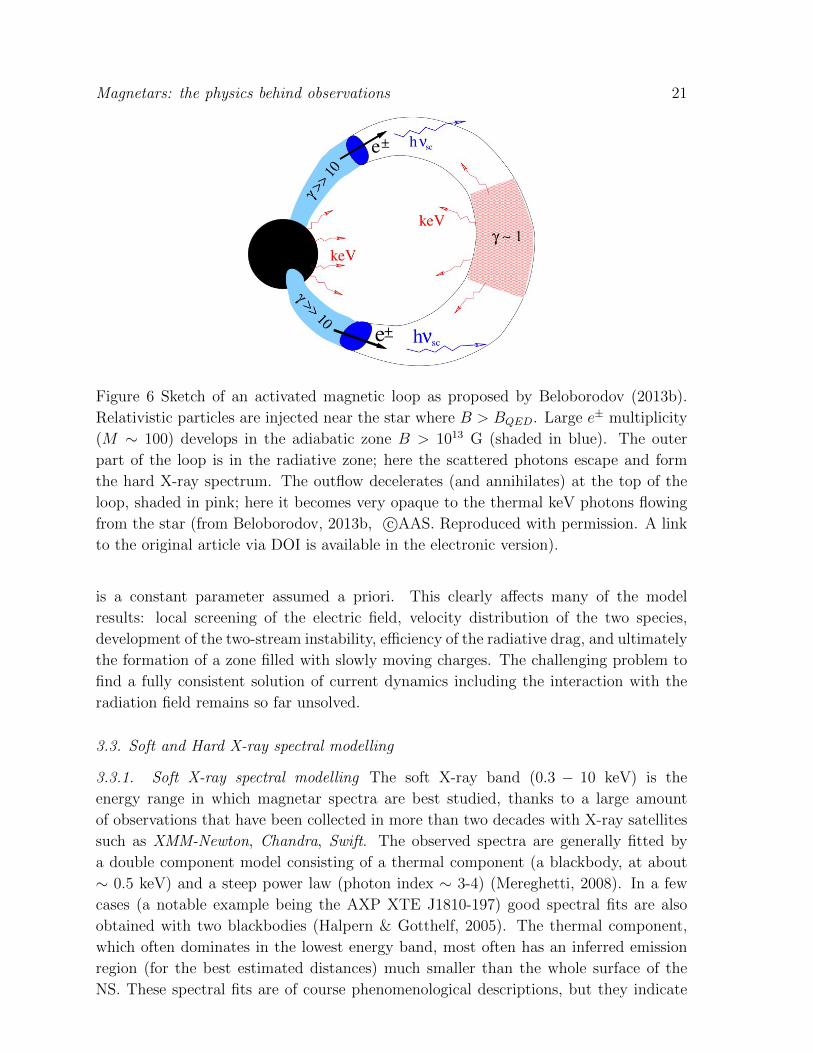
Figure 6 Sketch of an activated magnetic loop as proposed by Beloborodov (2013b).
Relativistic particles are injected near the star where B > BQED. Large e± multiplicity
(M ∼ 100) develops in the adiabatic zone B > 1013 G (shaded in blue). The outer
part of the loop is in the radiative zone; here the scattered photons escape and form
the hard X-ray spectrum. The outflow decelerates (and annihilates) at the top of the
loop, shaded in pink; here it becomes very opaque to the thermal keV photons flowing
from the star (from Beloborodov, 2013b, c©AAS. Reproduced with permission. A link
to the original article via DOI is available in the electronic version).
is a constant parameter assumed a priori. This clearly affects many of the model
results: local screening of the electric field, velocity distribution of the two species,
development of the two-stream instability, efficiency of the radiative drag, and ultimately
the formation of a zone filled with slowly moving charges. The challenging problem to
find a fully consistent solution of current dynamics including the interaction with the
radiation field remains so far unsolved.
3.3. Soft and Hard X-ray spectral modelling
3.3.1. Soft X-ray spectral modelling The soft X-ray band (0.3 − 10 keV) is the
energy range in which magnetar spectra are best studied, thanks to a large amount
of observations that have been collected in more than two decades with X-ray satellites
such as XMM-Newton, Chandra, Swift. The observed spectra are generally fitted by
a double component model consisting of a thermal component (a blackbody, at about
∼ 0.5 keV) and a steep power law (photon index ∼ 3-4) (Mereghetti, 2008). In a few
cases (a notable example being the AXP XTE J1810-197) good spectral fits are also
obtained with two blackbodies (Halpern & Gotthelf, 2005). The thermal component,
which often dominates in the lowest energy band, most often has an inferred emission
region (for the best estimated distances) much smaller than the whole surface of the
NS. These spectral fits are of course phenomenological descriptions, but they indicate

Magnetars: the physics behind observations 22
that, although the emission is mostly thermal, it is more complex than a blackbody at
a single temperature. It is also interesting to note that when one compares the average
temperature (from the thermal luminosity) of magnetars with those of other classes of
isolated neutron stars, there is a clear correlation between temperature and magnetic
field (Aguilera et al., 2008) and the magnetars are systematically more luminous than
rotation-powered neutron stars of comparable characteristic age (see a discussion in
Mereghetti et al., 2014). The morphology of the soft X-ray pulse profiles of magnetars
is varied. A few sources exhibit an (almost symmetric) double-peaked light curve (e.g.
1E 2259+586 and 4U 0142+0162; Patel et al., 2001; Woods et al., 2004; Rea et al.,
2007c) with pulsed fraction in the range 10− 20%. For most other magnetars, instead,
the pulsed component is single peaked and often the pulsed fraction is high (see e.g.
1E 1048.1-5937, XTE J1810-197, 1E 1547.0-5408, SGR 0418+5729, and SGR J1822.3-
1606 Tam et al., 2008; Bernardini et al., 2009, 2011a; Halpern & Gotthelf, 2011; Dib
et al., 2012; Rea et al., 2013a, 2012a). As originally suggested by Marsden & White
(2001), as a general rule sources with larger spin-down rate have smaller photon index
in the soft X-ray band. This fact has been confirmed with more recent data and it
appears to be valid for both persistent and transient sources in outburst, but only for
rotational frequencies derivatives ν & 10−14 s−2, and with some exceptions (including
the transients in outbursts and the recently discovered low-B magnetars, see Sec. 4.2
and Mereghetti et al., 2014). The long term evolution of the power law component and
timing properties of SGR 1806-20 indicates that the same correlation between spectral
hardness and average spin-down rate also holds for a single source (Mereghetti et al.,
2005b). On the wake of this, other correlations between the spectral hardness and the
timing properties have been investigated. In particular, that with the dipole strength
Bdip ∝ (PP )1/2 appears the most robust (Kaspi & Boydstun, 2010).
It has been widely suggested that the blackbody plus power law spectral shape
that is observed below ∼ 10 keV in magnetars’ spectra may be accounted for if
the soft, thermal spectrum emitted by the star’s surface is distorted by resonant
cyclotron scattering (RCS) onto the magnetospheric charges. Since electrons permeate a
spatially extended region of the magnetosphere, where the magnetic field varies, resonant
scattering is not expected to give rise to narrow spectral lines (corresponding to the
successive cyclotron harmonics), but instead to lead to the formation of a hard tail
superimposed on the seed thermal bump. This model is also in general agreement with
the hardness-P or hardness-magnetic field correlation mentioned above: stronger and
more twisted fields yield a larger spin down rate as well a higher magnetospheric charge
density that in turn produces a harder spectral tail. In recent years, several teams have
tested the resonant cyclotron scattering model quantitatively against real data in the
soft X-ray range, using different approaches and under different approximations. The
first, seminal attempts in this direction were presented by Lyutikov & Gavriil (2006) who
developed a very simplified one dimensional model. They assumed that seed photons
are emitted by the NS surface with a blackbody spectrum, and propagate backward and
forward in the radial direction. A thin, plane parallel magnetospheric slab, permeated

Magnetars: the physics behind observations 23
by a static, non-relativistic, warm medium at constant electron density is assumed to
exist above the star’s surface. Magnetic Thomson scattering occurs between photons
and the charges in the slab, and the process is computed by neglecting all effects of
electron recoil, as are those related to the current’s bulk motion. Despite being clearly
over-simplified, this model has the main advantage of being semi-analytical and, when
systematically applied to X-ray data, has proved successful in capturing at least the
gross characteristics of the observed soft X-ray spectrum (Rea et al., 2007a,b, 2008).
The same model has been extended by Guver et al. (2007), who relaxed the
blackbody approximation for the seed surface radiation and made an attempt to include
atmospheric effects, treating the star’s surface emission like that of a passive cooler, i.e.
using an atmospheric code akin to those originally developed for sources with purely
thermal emission (e.g. Zavlin et al., 1996; Zane et al., 2001; Ozel, 2003; Potekhin, 2014,
and references therein). This is a quite drastic and somewhat unphysical simplification
for sources like magnetars, which are characterized by strong magnetospheric activity
leading to particle back-bombardment, heat deposition and other similar effects. Despite
this, the model has been applied to real data in an attempt to estimate the surface
magnetic field through data fitting of the soft X-ray continuum (Guver et al., 2008,
2011; Ozel, 2013). At present the problem appears to be still open: while it is commonly
recognized that thermal radiation from the star’s surface is likely to be different from
a simple blackbody, either because of local reprocessing by some sort of (non passive)
atmosphere or because the surface itself may be in a condensed state, a self consistent
inclusion of these effects in numerical models has not yet been carried out.
In order to perform a more physical, 3-D treatment of the RCS problem, the most
suitable approach is to make use of a Monte Carlo technique, which is quite easy to
code, and, when dealing with purely scattering media at moderate optical depths,
relatively fast. The Monte Carlo scheme allows one to follow individually a large sample
of photons, treating probabilistically their interactions with charged particles. These
simulations have been developed by only a few teams (Fernandez & Thompson, 2007;
Nobili, Turolla & Zane, 2008a). The numerical codes that have been developed are
completely general, inasmuch that in principle they can handle different 3-D geometries
(so highly anisotropic thermal maps and magnetic fields) and different radiative models
of surface emission. On the other hand, since our understanding of these ingredients is
still limited, in order to minimize the number of degrees of freedom, simulations were
computed by assuming, for simplicity, that i) the whole surface emits isotropically as
a blackbody at a single temperature, ii) the magnetic field is a force-free, self-similar,
twisted dipole and iii) the electron velocity distribution is assumed a priori (see Sec. 3.2).
Besides, resonant scattering was treated in the magnetic Thomson limit, which allows
one to account for polarization (under the two stream approximation) but it neglects
electron recoil, limiting the applicability of the results to energies up to a few tens of keVs
(hν < mc2/γ keV, B/BQ < 10). By comparing the results from the different teams, one
may conclude that, while the general effects induced by magnetospheric RCS on primary
thermal photons (i.e. the formation of a “thermal-plus-power-law” spectrum) are not

Magnetars: the physics behind observations 24
Figure 7 Left: Computed spectra from Monte Carlo simulations for B = 1014 G,
kT = 0.5 keV, kTe = 30 keV, ∆φ = 1 and different values of βbulk: 0.3 (dotted), 0.5
(short dashed), 0.7 (dash-dotted) and 0.9 (dash-triple dotted). The solid line represents
the seed blackbody and spectra are computed at a magnetic colatitude: Θs = 64◦.
Right: Spectrum from a single emitting patch on the star surface. The line of sight is
at Θs = 90◦ and Φs = 20◦ (dotted line), 140◦ (dashed line) and 220◦ (dash-dotted line).
These three values correspond to having the emitting patch in full view (seen nearly
face on), partially in view and screened by the star. The solid line represents the seed
blackbody (readapted from Nobili, Turolla & Zane, 2008a, with OUP permission).
very sensitive to the assumed particle velocity distribution, the details of the spectral
shape do, and, as we will discuss later on, this is particularly critical for the model
predictions in the hard X-ray band. Nevertheless, in the soft X-ray band, for several
combinations of the parameters, the general shape of the continuum is that of a thermal
bump and a high-energy tail (see Fig. 7), which is in agreement with what is observed
in the XMM-Netwon and Chandra spectra (below ∼ 10 keV). The spectral index of
the high energy tail changes with the parameters and, in particular, harder spectra are
found for increasing twist angle. This was invoked as a possible mechanism to explain
the correlated flux-hardening long term variations in some sources (e.g. Thompson,
Lyutikov & Kulkarni, 2002; Mereghetti et al., 2005b; Rea et al., 2005; Campana et al.,
2007; Nobili, Turolla & Zane, 2008a).
The numerical spectra computed by Nobili, Turolla & Zane (2008a) have been

Magnetars: the physics behind observations 25
Figure 8 Fit of the XMM-Newton spectra of the AXP 1E 1048-5937 and SGR 1806-20
with the NTZ model. The panels show a joint fit of spectra taken at three different
epochs and the fitting has been restricted to the 1− 10 keV range (adapted from Zane
et al., 2009, with permission).
implemented in XSPEC and successfully fit the XMM-Newton spectra of most of the
magnetar sources in quiescence (NTZ model, Zane et al., 2009, see also Fig. 8). This
allows one to derive of the gross characteristics of the magnetosphere in such sources
and to obtain a better estimate of the thermal component.
Interestingly, in the case of two sources, 1E 2259+586 and 4U 0142+614 , it was not
possible to find a satisfactory fit with the NTZ XSPEC model although these spectra
were fitted by the simplified 1-D model (Rea et al., 2007a). As suggested in Zane
et al. (2009), a plausible cause is that the BB peak appears to be less prominent to
the observer because the region that emits the soft seed photons is not completely in
view. By modelling the RCS spectra under the assumption that photons are emitted
by a single surface patch it is immediately clear that the effects of the different viewing
angle on the spectrum are dramatic. When the emitting patch is in full view both
the primary, soft photons and those which undergo repeated resonant scattering reach
the observer, and the spectrum is qualitatively similar to those presented earlier on,
with a thermal component and an extended power-law-like tail. If on the other hand
the emitting region is not directly visible, no contribution from the primary blackbody
photons is present (see Fig. 7, right panel). The spectrum, which is made up only
by those photons which after scattering propagate “backwards”, is depressed and has
a much more distinct non-thermal shape, much more similar to the one observed in
1E 2259+586 and 4U 0142+614 .
Unfortunately, in a realistic situation the thermal surface map is expected to be
complex and it cannot always be reconstructed by fitting the X-ray spectrum alone. As
discussed in Albano et al. (2010, see also Bernardini et al. 2011a), a better strategy
consists of performing a simultaneous fitting of the energy-resolved X-ray lightcurves,
since they carry a much more defined imprint of the surface thermal distribution (see
Sec. 4 and Fig. 18 therein). While this is not possible for all sources, transient AXPs, for
which a set of observations spread over few years and at different flux levels are available,
provide a spectacular laboratory for this exercise. Albano et al. (2010) were the first (and
so far the only) team to present a comprehensive study of the outburst decay of the two
transient AXPs (TAXPs) XTE J1810-197 and CXOU J164710.2-455216, reproducing
both the spectral and pulse profile evolution based on fits with three-dimensional Monte
Carlo simulations. This allowed them to prove the presence of distinct temperatures
zones (up to three) at the star’s surface, some of them possibly heated by the energy

Magnetars: the physics behind observations 26
released during the outburst, to model their evolution during the outburst decay, and
to constrain the viewing geometry of the sources, i.e., the inclination of the line of sight
and the magnetic axis with respect to the rotation axis.
A similar conclusion concerning the need to investigate the pulse profile behaviour
when trying to reconstruct inhomogeneous surface thermal maps was reached by Perna
et al. (2013). These authors considered the case in which the temperature anisotropy is
observed also in quiescence, as is expected if complex magnetic field components in the
NS crust and interior make heat transport from the core outward highly anisotropic.
They used state-of-the art numerical codes (Vigano et al., 2012, 2013) for the coupled
magneto-thermal evolution of neutron stars and computed the expected pulse profiles
and spectra (under the assumption of blackbody emission) for a range of magnetic
configurations. Particularly compelling is the finding that, while in presence of purely
dipolar fields the pulse profile is always double-peaked and with a relatively low pulsed
fraction, when strong toroidal components are present the pulse fraction can exceed 50–
60% and the pulse profile can be single peaked (as often observed in AXPs and SGRs).
Moreover, if the simulated spectra are fitted with a highly absorbed BB model, only
relatively concentrated hot peaks are visible, so that the inferred BB radius turns out
to be much smaller than the NS radius (even as low as 1-2 km, see Fig. 9). Strong
toroidal crustal B-field components, coupled with large absorption column densities
(> 1022 cm−2, see e.g. Esposito et al. 2008), can therefore explain the small caps
very often required by the spectral fits of AXPs and SGRs. Even smaller (sub–km)
hot spots are measured in certain sources (e.g. CXO J164710.2-455216, see e.g. Israel
et al. 2007), but they look more likely to be produced by particle bombardment and
heat deposition from currents highly concentrated in twisted magnetic polar bundles
(Beloborodov, 2009; Turolla et al., 2011) which emerge from the crust, rather than
anisotropic internal heat transfer. In this respect it is worth mentioning the work
by (Bucciantini et al., 2015), who presented a comprehensive and detailed parameter
study, in general relativity, of the role that the current distribution investigating several
equilibrium global field configurations derived using a Grad-Shafranov approach (Pili et
al., 2015). These authours found that the structure and strength of the magnetic field at
the surface is strongly influenced by the location and distribution of currents inside the
star, with the result that the surface field can easily be dominated by higher multipoles
than the dipole. This means that in some cases the magnetic field at the equator can
be even much higher or much smaller than the value of the field at the pole and implies
that signatures observed in features originating at or near the surface might differ from
the expectations of a dipole dominated model, while observations of processes related
to the large scale field, as spin-down, will not (see also the discussion in Sec. 4.2).
3.3.2. Hard X-ray spectral modelling Hard X-ray observations with the INTEGRAL,
RXTE and Suzaku satellites have shown that in some magnetar candidates (namely 4U
0142+614, 1RXS J1708-4009, 1E 1841-045, 1E 2259+586, SGR 1806-20, SGR 1900+14;
Kuiper et al., 2004, 2006; Mereghetti et al., 2005a; Molkov et al., 2005; Gotz et al., 2006;

Magnetars: the physics behind observations 27
Figure 9 Temperature surface distribution for sources with a magnetic field at birth
which has both a poloidal and a toroidal component. For ages typical of magnetars
(104 − 105 yrs) the expected thermal map consists of a hot polar spot and an extended
colder region; the latter may be undetected if the source is highly absorbed (from Perna
et al., 2013, with OUP permission).
Enoto et al., 2011) a large fraction of the total quiescent flux is emitted at energies well
above ∼ 20 keV. These “hard” tails have a non-thermal (PL) character, and extend
up to a few hundreds of keV. Pulsed phase spectroscopy has been performed for a few
sources, although with limited statistics due to the low number of counts, revealing that
the emission is likely characterized by different components that emerge at different,
and sometimes only in limited, phase intervals (den Hartog et al., 2008a,b).
This discovery came quite unexpectedly and suggests that a new magnetar
characteristics may be that a considerable fraction of their bolometric luminosity is
emitted in the hard, rather then in the soft X-rays. In fact, limits on the non-detected
sources are not deep enough to exclude the presence of a similar hard tail. The first
observations of emission at > 20 keV revealed a difference between the (at that time
separated) AXPs and SGRs (Gotz et al., 2006): in the Integral and RXTE data the
AXPs’ hard power law is considerably harder than that observed below 10 keV, while
SGRs’ hard spectra are considerably steeper. More recent observations with NuStar
indicate that the division is not as sharp and magnetar sources show a varied behaviour,
which is consistent with the fact that SGRs and AXPs are now considered a single class
(An et al., 2014b). NuStar, which has a sensitivity roughly two orders of magnitude
better than previous missions in this energy band and a high angular resolution, is
currently observing a selected sample of magnetars as part of its priority A targets (see
An et al., 2014b, for a review and references therein). One of the major goal is to study
the spectral location of the soft/hard X-ray turnover, which is expected to correlate with
Bdip (Kaspi & Boydstun, 2010). Interestingly, while for some sources the new NuStar

Magnetars: the physics behind observations 28
Figure 10 Left: XMM-Newton and INTEGRAL spectra of magnetars (from Gotz et al.,
2006, reproduced with permission c©ESO). Note the different behavior of SGRs (two
top panels) and AXPs: in the latter sources the spectra turn upward above 10 keV,
while in the SGRs the spectra steepen. Right: Broad band spectral energy distribution
of 4U 0142+614 (from Kuiper et al., 2006, c©AAS. Reproduced with permission. A link
to the original article via DOI is available in the electronic version). Both the total and
the pulsed emission are indicated. Both figures are readapted from Mereghetti (2008),
with kind permission from Springer Science and Business Media.
results are in agreement with the Integral and RXTE ones, in some other cases (e.g.
1E 2259+586) it appears evident that the hard band spectrum for the total emission is
not as hard as the pulsed one. Despite that, the analysis of 1E 2259+586 data confirmed
that an additional component, such as a power law, is needed to describe the emission
in the hard X-ray band (Vogel et al., 2014). This suggests that at least in some sources
the non thermal mechanisms responsible for the emission in the soft and hard X-rays
are distinct, or that the charge properties in the two emission regions are different.
Observations at higher energy with Comptel and Fermi LAT failed to detect
magnetar emission, implying the presence of a spectral break above a few hundred
keV (Kuiper et al., 2006; den Hartog et al., 2006; Sasmaz Mus & Gogus, 2010). The
only exception reported so far is a possible Fermi Large Area Telescope (LAT) detection
of γ-ray pulsations above 200 MeV from the AXP 1E 2259+586 (Wu et al., 2013) which
however still needs a robust confirmation. Some example of few magnetar spectral
energy distributions in the soft/hard X–rays are shown in Fig. 10.
The mechanism responsible for the high energy emission is still poorly understood,

Magnetars: the physics behind observations 29
at least in its quantitative details. High energy emission from currents moving in the
highly magnetized magnetosphere is expected for a number of reasons. Thompson
& Beloborodov (2005) originally suggested that hard X-rays may be produced either
by thermal bremsstrahlung in the surface layers heated by returning currents, or by
synchrotron emission from pairs created higher up (∼ 100 km) in the magnetosphere.
A further possibility, according to which the soft γ-rays may originate from resonant
up-scattering of seed photons on a population of highly relativistic electrons, has been
proposed by Baring & Harding (2005, 2008). As mentioned earlier, most of the RCS
models computed with Monte Carlo simulations are based on the assumption that
scattering can be treated in the Thomson approximation, which limits their validity
up to a few tens of keV. Instead, a proper investigation of the effects of electron recoil
and of multiple scatterings from high energy photons demand the use of the full QED
cross section. Relatively simple expressions of the QED cross section at resonance, in a
form that is simple to include in Monte Carlo simulations, have been computed by Nobili,
Turolla & Zane (2008b) and a few examples of the emerging spectra, computed under
the assumption of self-similarly distributed twist and constant electron velocity, have
been discussed in Zane et al. (2011a). These simulations show that, if magnetospheric
electrons are mildly relativistic, when considering self-consistently electron recoil and
QED effects the spectrum exhibits a break at a few hundred of keV. This is due to the
fact that, in order to populate the hard energy tail, soft seed photons need to experience
a series of successive scatterings, each characterized by a limited energy gain because
the Lorentz factor of electrons is only γ ∼ a few. In parallel, the efficiency of the
QED cross section decreases with increasing energy (or, since the process is resonant,
with increasing magnetic field) and the combination of these two effects leads to the
appearance of the spectral break. The energy of the break depends on the effect of the
cumulative scatterings and is sensitive to the details of the magnetic field topology and of
the currents’ distribution and therefore cannot be predicted a priori nor estimated using
a simple expression. On the other hand, in the case in which magnetospheric electrons
are ultra-relativistic, the energy gain per scattering is so large that the hard tail becomes
efficiently populated after just a few scatterings. In this case, now independently of the
details of the cross section and magnetic topology, the spectral tail is predicted to be
quite flat and unbroken, even up to > 1000 keV (see Fig. 11).
Although these studies are extremely useful in shedding light on the basic behaviour
of the QED scattering process, the assumptions of constant charge velocity and self-
similar magnetic twists are clearly two major oversimplifications. This is crucial when
trying to mimic the hard X-ray emission, since the responsible emitting region is likely
to constitute quite a large portion of the whole magnetosphere. We already mentioned
that deep INTEGRAL observations of two AXPs 1RXS J1708-4009 and 4U 0142+61
have revealed several different pulse components (at least three) in the hard X-rays,
with genuinely different spectra (den Hartog et al., 2008a,b) and a quite spectacular
phase-dependence. The hard X-ray spectrum gradually changes with phase from a soft
to a hard power law, the latter being significantly detected over a phase interval covering

Magnetars: the physics behind observations 30
Figure 11 Monte Carlo spectra for B = 1014 G and ∆φ = 1 computed by using the
full QED expression of resonant scattering. Left: mildly relativistic electrons (γ = 1.7).
Right: highly relativistic electrons (γ = 22) (reprinted from Zane et al., 2011a, Copyright
2011, with permission from Elsevier).
∼1/3, or more, of the spin period. This richness in the phenomenology requires more
complex magnetospheric topologies to be explained. Unfortunately, despite many efforts
having been devoted to the development of techniques for solving the force-free equation,
∇×B = α(x)B, no general, affordable method has been presented so far. Pavan et al.
(2009) developed a general method to generate twisted, higher-order multipoles solving
the Grad-Shafranov equation, and analyzed in detail quadrupolar and octupolar fields.
The case of an octupolar field has a special interest because it can be used to mimic
a twist localized in a region close to the magnetic pole(s), and hence to investigate
the consequence in the expected spectra. Model (Monte Carlo) spectra and lightcurves
have been presented for the cases in which the twist is confined to one or both polar
regions (each region has semi-aperture of ∼ 60 deg), by assuming that only the polar
lobes have a non-vanishing shear while the equatorial belt is potential. Interestingly,
a configuration with a twist confined to a single lobe has been found to be capable of
qualitatively reproducing the main features of the high-energy emission observed with
INTEGRAL from the AXPs 1RXS J1708-4009 and 4U 0142+61, in particular the large
variation in the pulsed fraction at different energy bands, and a hard tail which is quite
pronounced at the peak of the pulse but depressed by almost an order of magnitude at
pulse phases close to the minimum of the hard X-ray lightcurve.
More recently, an alternative to the (mathematically simple) self-similar models,
has been presented by Vigano et al. (2012), who discussed the effects of more
realistic magnetic field geometries on the synthetic Monte Carlo spectra. They
presented a numerical method to build general force-free field magnetic configurations,
starting from an arbitrary, non-force-free poloidal plus toroidal field and employing
artificial dissipation to remove the non-parallel currents. In particular, they considered
configurations in which the currents are concentrated in a bundle along the polar axis,
as expected for a spatially-limited twist. In this case the pulse fraction is larger with

Magnetars: the physics behind observations 31
Figure 12 Left and center panel: magnetic field and current distribution for a high
helicity model with current and twist concentrated in a closed bundle near the equatorial
region and a j-bundle near the southern semi-axis. This configuration is likely more
realistic than the self-similar models, since currents are more concentrated near the
axis. The two panels show | ~B| (grey logarithmic scale) with superimposed the scattering
surfaces for photons of 1, 3 and 5 keV and the current intensity | ~J |/c (gray linear scale)
in units of 1014 G/rNS. Right: Corresponding synthetic spectra computed with a Monte
Carlo simulation. Different curves correspond to four different viewing angles; the seed
blackbody is shown for comparison as a solid line. (readapted from Vigano et al., 2012,
with permission; a link via DOI to the original version is available in the electronic
version of this paper).
respect to that of self-similar models, and the spectrum observed at different angles
varies in a much more irregular way (see Fig. 12). Instead of a simple PL, it shows
different spectral bumps the relative importance of which can vary by one order of
magnitude or more at different colatitudes. The different spectral components inferred
from the data may therefore be due to these bumps. Even if a real fit has not been
attempted, we may speculate that this is qualitatively in line with the observations of
the AXPs 1RXS J1708-4009 and 4U 0142+61.
As mentioned earlier, a further poorly known ingredient of all these simulations is
the charge velocity distribution and probably the most detailed solutions published have
been presented by Beloborodov (2013a,b). In this scenario, the electron-positron flow
decelerates as it propagates away from the neutron star surface (due to Compton drag
in the resonant scattering region), then it reaches the top of the magnetic loop where it
annihilates. While computed with a Monte Carlo simulation, the corresponding spectra
show a distinct peak at E > 1 MeV (so far unobserved), the position of which is however
strongly dependent on the viewing angle (or, equivalently, on the magnetic colatitude
at which the spectrum is emitted, see Fig. 13).
A well defined change in the power law slope from soft to hard X-rays is seen, which
makes these spectral models incapable of explaining observations of sources that have
a similar slope below and above ∼ 10 keV (historically these were referred as SGR-like

Magnetars: the physics behind observations 32
Figure 13 Left: Spectrum emergent from scattering onto charges populating an
axisymmetric j-bundle. Different lines represent the spectrum as observed at four
different angles with respect to the magnetic axis: 15o, 30o, 60o, and 90o. The spectrum
is normalized to the total luminosity of the j-bundle. (from Beloborodov, 2013b, c©AAS.
Reproduced with permission. A link to the original article via DOI is available in the
electronic version).
spectra), but instead in good qualitative agreement with the observed spectra in which
a marked turnover is present (historically, AXP-like spectra). In an attempt to perform
a quantitative comparison without to resort to the time-consuming computation of a
complete table of Monte Carlo models, Hascoet et al. (2014) developed a simplified model
by assuming the same charge velocity distribution but by computing the spectra through
a simple calculation of the angle-dependent emissivity alone. The magnetosphere is
assumed to be axysymmetric and dipolar, apart from the presence of a current-carrying
region (the j-bundle), which is filled with the electron-positron flow. These spectra have
been then applied to multi-year hard X–ray observations of 4U 0142+61, 1RXS J1708-
4009 and 1E 1841-045, finding that they successfully reproduce the emission observed
above ∼ 10 keV in both the phase-average and phase-resolved spectra. Unfortunately,
the authors found that the model predictions cannot be self consistently applied to
explain also the data below 10 keV (probably because of the lack of the particle back-
bombardment effects in the simulation). These predictions have therefore been ignored
in the fits and instead a blackbody component(s) was used to account for the soft X-
ray part of the spectrum. A concern regarding these fits is the fact that the spectra
used by Hascoet et al. (2014) do not include photon splitting, which is the main factor
responsible for the bump visible in the Monte Carlo spectra at ∼ 1 MeV (Beloborodov,
2013b). Although the simplified and complete calculations are in good agreement below
∼ 400 keV, they are expected to be markedly different at higher energies. Actually,

Magnetars: the physics behind observations 33
there is no guarantee that, should the spectra be computed self-consistently with the
Monte Carlo code, the high energy CGRO-Comptel upper limits are not violated (either
always or for the derived geometry). This casts some doubts on the robustness of the
study and on the constraints on the viewing geometry reported by Hascoet et al. (2014)
fitting only the hard X-ray part of the spectrum.
It is interesting to note that spectra presented by Wadiasingh et al. (2013), using
a new Sokolov and Ternov formulation of the QED Compton scattering cross section in
strong magnetic fields and accounting for spin-dependent effects at resonance, also show
a spectral cut-off whose energy is critically dependent on the observer viewing angles
and electron velocity, with substantial emission expected up to 1 MeV except for very
selected viewing angles.
At the present, unfortunately, what causes the high energy emission and its richness
in phenomenology is still an open issue: models have been computed, but they depend
dramatically on a large number of degrees of freedom for the magnetospheric setting at
large scale. New and future missions such as Astro-H, NuSTAR, and possibly LOFT
would provide the possibility of collecting simultaneous soft and hard spectra, to study
the correlation between the variability in the two bands, to perform high resolution
pulsed phase spectroscopy and to reveal the detail of the slope turn-over (when present)
in the soft-to-hard emission. In turn, this will provide a powerful tool to break the
model degeneracy and an unprecedented insight into the details of the field and current
distributions.
3.4. X-ray polarization
As discussed in Sec. 3.3.1, comparison of RCS models with the soft X-ray spectral data
of magnetar candidates has proved quite successful. However, spectroscopy alone cannot
provide complete information on the physical properties of the magnetosphere, due to
the inherent degeneracy in the RCS model parameters. Moreover, computed spectra
are rather insensitive to the source geometry, although in principle they do depend on
the angles that the line of sight and the magnetic axis make with the star’s rotation
axis (Nobili, Turolla & Zane, 2008a; Zane et al., 2009). Although a simultaneous fit of
both the (phase-averaged) spectrum and the pulse profile is effective in this respect, at
least for TAXPs (Perna & Gotthelf, 2008; Albano et al., 2010; Bernardini et al., 2011a),
polarization measurements at X-ray energies would provide an entirely new approach
to the determination of the physical parameters in magnetar magnetospheres.
X-ray radiation from a magnetar is expected to be polarized for essentially three
reasons: i) primary, thermal photons, coming from the star’s surface, can be intrinsically
polarized, because emission favors one of the modes with respect to the other; ii)
scattering can switch the photon polarization state; and iii) once the scattering depth
drops, the polarization vector changes as the photons travel in the magnetosphere (the
so called “vacuum polarization”, Heyl & Shaviv, 2000, 2002, see also Harding & Lai
2006).

Magnetars: the physics behind observations 34
Figure 14 Contour plots for number of counts (in arbitrary units; left column),
polarization fraction (middle column) and polarization angle (right column) as functions
of the photon energy and cos θ for different values of the twist angle and the electron
bulk velocity: ∆φ = 1.3 rad, β = 0.3 (top row) and ∆φ = 0.7 rad, β = 0.4 (bottom row).
In both cases it is Bp = 5× 10¹⁴ G (from Taverna et al., 2014, with OUP permission).
Although a preliminary analysis was already contained in Fernandez & Thompson
(2007) and Nobili, Turolla & Zane (2008a), a detailed study of the polarization properties
of magnetar radiation in the X-ray band has been presented by Fernandez & Davis (2011)
and, more recently, by Taverna et al. (2014), by means of Monte Carlo simulations.
Phase-averaged as well as phase-resolved results indicate that the linear polarization
fraction ΠL and the polarization angle χpol, are very sensitive to the magnetospheric
twist angle ∆φ and the charge velocity β, and also to the geometric angles χ and ξ.
This allows one to remove the ∆φ-β degeneracy which spectral measures alone cannot
disambiguate. An example is shown in Fig. 14 where the photon spectrum, polarization
fraction and polarization angle are plotted as functions of viewing angle and energy
for two choices of the model parameters. While the photon spectrum is practically
the same, the pattern of ΠL and especially χpol is markedly different in the two cases.
According to the simulations by Taverna et al. (2014), polarimetric measurements in
bright magnetar candidates, like the AXP 1RXS J1708-4009, are within reach of recently
proposed polarimeters which should hopefully fly in future missions.
3.5. IR/optical emission
As mentioned in Sec. 1, variable IR counterparts have now been identified, or in some
cases proposed, for a number of magnetars (Mereghetti, 2011; Israel & Rea, 2014). In
addition, three magnetars have been detected in the optical band, the two AXPs 4U
0142+61 (Hulleman et al., 2000) and 1E 1048.1-5937 (Durant & van Kerkwijk, 2005),
and the SGR 0501+4516 (Fatkhullin et al., 2008; Dhillon et al., 2011). The origin of this
emission is still under debate, and the main dispute is whether it is due to the presence

Magnetars: the physics behind observations 35
of a fossil disk (Perna et al., 2000) or if it has a magnetospheric origin (Eichler, Gedalin
& Lyubarsky, 2002; Beloborodov & Thompson, 2007).
AXP 4U 0142+61 is the only persistent magnetar for which the optical/near IR
(NIR) spectrum was measured, although the faintness of the source required extensive
observational data (Hulleman et al., 2000). In the case of this source, an IR “excess“
(or “flattening“) was clearly detected with respect to the extrapolation of the additional
black body used to account for the optical emission (Israel et al., 2004, 2005a). This may
suggest that the IR emission is due to a distinct spectral component, a conclusion that
might well hold also for other AXPs, considering the similarity of their IR magnitudes
and FX/FIR ratios (Durant et al., 2011).
The optical/NIR spectrum of 4U 0142+614 was found to be well fitted by a multi-
temperature (700-1,200 K) thermal model, leading to the suggestion it originates in an
extended disk or shell (Wang et al., 2006). If this detection of a fallback disk is real,
it would be the the first direct evidence for supernova fallback in any context. On the
other hand, disks may then be ubiquitous while, despite intense campaigns, no similar
direct evidence has been found for other sources (see also Posselt et al., 2014, for a
report on recent deep limits on fallback disks). The only indirect evidence is one source,
in which there is a detected correlation between the NIR and X-ray fluxes (Tam et al.,
2004), which, as pointed by Wang et al. (2006), may indicate that the IR emission arises
in an X-ray-heated debris disk.
On the other hand, very deep optical and NIR observations of the field of the low-B
magnetar SGR 0418+5729, which is the nearest and least extincted magnetar known,
failed to detect the source counterpart (Durant et al., 2011). Shallower observation of
the field of SGR 0418+5729 with the new Gran Telescopio Canarias 10.4-m telescope
and with the William Herschel Telescope where also taken closer to the onset of the
outburst (Esposito et al., 2010; Rea et al., 2013a) and only gave upper limits on the
countarpart. This negative result is in better agreement with a magnetospheric origin
interpretation, in which case the IR/optical flux is expected to be fainter for lower field
strengths. Moreover, a magnetospheric scenario is more likely to explain the fact that,
when detected, the observed optical emission is pulsed at the pulsar period, with pulsed
fractions > 50%, i.e., higher than in soft X-rays (Kern & Martin, 2002; Dhillon et al.,
2009, 2011).
Magnetospheric emission in the IR/optical is expected from the inner region of
the magnetosphere (Beloborodov & Thompson, 2007; Zane et al., 2011b). As discussed
in Sec. 3.2, this region is expected to be pair-dominated, and the Lorentz factor of
the electrons and positrons is likely to be frozen at the threshold for pair production
(γ ∼ 500 − 1000). In order to estimate the amount of curvature radiation, Zane et
al. (2011b) developed a simple geometrical model accounting for misalignment between
the observer line of sight and the magnetic axis. Although the model is too simple to
allow for a proper spectral fitting, it is detailed enough to make a prediction about the
energetics and the computation indicates that curvature radiation is sufficient to explain
the amount of observed IR/optical flux, at least if a particle bunching mechanism is

Magnetars: the physics behind observations 36
Figure 15 Model spectra for different values of the viewing angle and B = 4.3× 10¹⁴ G.
The XMM-Newton X-ray spectrum of 1RXS J1708-4009 is from Rea et al. (2008, red solid
line). The AXPs IR/optical data are from Durant & van Kerkwijk (2005, 4U 0142+614
and 1E 1048-5937) and Mignani et al. (2007, XTE J1810-197 and 1E 2259+586). The
adopted distances for de-reddening are 5 kpc (4U 0142+614, 1RXS J1708-4009), 3 kpc
(1E 1048-5937, 1E 2259+586), 4 kpc (XTE J1810-197), 8.5 kpc (1E 1841-045). Curvature
emission spectra have been computed accounting for particle bunching (Fig. 2 from Zane
et al., 2011b, With kind permission from Springer Science and Business Media) .
efficient (see also Beloborodov & Thompson 2007 and see Fig 15). This is not unlikely,
since many models have been suggested to explain the origin of the interactions which
push particles together and can lead to the formation of bunches of charged particles
localized in phase-space. The most promising explanation seems to be connected with
plasma instabilities, like the two-stream (electron-positron/electron-ion) instability. We
notice that this mechanism does not affect the emission in other bands. In fact, in order
the process to be effective, it has to have N = nel3B > 1, where lB is the size of the bunch
and ne is the electron density, which in turns means that only emission at frequencies
ν < νco = n1/3e c is efficiently amplified. Also, a low-energy cut-off is present because of
the strong absorption below the electron plasma frequency.
Israel et al. (2005b) proposed a link between the IR and hard X-ray spectrum
of AXPs, and correspondingly between AXPs/SGRs and radio-pulsars, based on the
analysis and comparison of their broad band energy spectra. These authors pointed out
that, similar to the case of a number of young radio pulsars such as the Vela, it is possible
to bridge the IR to γ-ray emission of AXPs with a power-law with index of about 0.5-0.6
(see Fig. 16). This peculiar similarity, for classes of neutron stars with otherwise quite
different emission properties, may naturally explain the IR excess or flattening in the
spectra of AXPs and points toward a similar origin for the less energetic bands and the
hard X-ray emission. This scenario may be unambiguously proven through simultaneous
studies of the correlated variability in the two bands, which have unfortunately so far
been hampered by the lack of gamma-ray observatories sensitive enough to these faint
sources.

Magnetars: the physics behind observations 37
Figure 16 Broad band energy spectrum of SGR 1806-20 (triangles), the AXP 1E
1841+045 (circles) and the radio pulsar Vela (squares). In the case of SGR 1806-20 and
1E 1841+045 high energy data are taken from Mereghetti et al. (2005a,b). Absorbed
and unabsorbed IR fluxes (AV = 29±2, 5th October 2004 NACO observation) are shown
in the case of SGR 1806-20, unabsorbed (AV = 13 ± 1) IR fluxes are instead reported
for the likely candidate of 1E 1841+045 (circles; Testa et al., 2008). All the data for
Vela are taken from Kaspi (2006). Solid curves (continuous, stepped and dot-stepped)
are the unabsorbed fluxes, for the blackbody plus power-law model used to fit the high
energy part of the spectra (courtesy G.L. Israel, from Israel et al., 2005b, reproduced
with permission c©ESO).
4. Transient Magnetars
The persistent X-ray emission of a number of SGRs/AXPs has been known to be variable
all along, with typical flux variations of a factor of a few over a timescale of days to
months, often in coincidence with periods of enhanced bursting activity (see Sec. 1; Rea
& Esposito, 2011). The first evidence that the luminosity of SGRs/AXPs can change
much more dramatically came from observations of SGR 1627-41 (Woods et al., 1999b)
and AX J1845.0-0300 (Torii et al., 1998; Vasisht et al., 2000, although the latter source
is only a candidate magnetar with no detection of P ).
It was not until 2002, however, that the existence of a new class of magnetar sources
with much more extreme variability was realized, thanks to the discovery of the first
transient AXP, XTE J1810-197 (Ibrahim et al., 2004). At present eleven transients are
known and, remarkably, they almost make up all of the new magnetars observed in the
last 10 yrs (the exception being CXOU J171405.7-381031, Halpern & Gotthelf, 2010).
The main properties of transient magnetars are listed in table 1+.
+ Only sources for which the peak luminosity is > 10 times the quiescent one have been included.

Magnetars: the physics behind observations 38
Table 1 Transient magnetar sources+
Source P P B D
(s) (10−11 s/s) (1014 G) (kpc)
CXOU J1647-4552 10.61 < 0.04 < 0.7 3.9
XTE J1810-197 5.54 0.77 2.1 3.5
SGR 0501+4516 5.76 0.59 1.9 52.0
SGR 0418+5729 9.08 0.0004 0.06 2.0
SGR 1833-0832 7.56 0.35 1.6 –
PSR 1622-4950 4.33 1.7 2.2 9.0
1E 1547-5408 2.07 4.77 3.2 4.5
Swift J1822.3-1606 8.4 0.02 0.14 1.6
SGR 1627-41 2.59 1.9 2.2 11.0
Swift J1834.9-0846 2.48 0.80 1.4 4.2
SGR J1745-2900 3.76 1.38 2.3 8.3
These sources are characterized by a sudden (≈ hrs) increase of the X-ray flux, by a
factor ≈ 10–1000 over the quiescent level, accompanied by the emission of short bursts.
This active phase, commonly referred to as an outburst, typically lasts ≈ 1 yr, during
which the flux declines, the spectrum softens and the pulse profile simplifies. Fig. 17
shows the decay of the X-ray flux for several transient magnetars. Some objects have
undergone repeated outbursts (SGR 1627-41, 1E 1547-5408) and the decay pattern
is often different from source to source (and even between outbursts from the same
source). Outbursts, besides revealing new magnetars which in quiescence are too faint
to be detectable, or which passed unnoticed among the host of unclassified, weak X-
ray sources, have also occurred in persistent sources like 1E 2259+586 or 1E 1048.1-
5937, although drawing a precise line between outbursts and less extreme variability is
somewhat haphazard. The group of transient sources also harbours the two peculiar
“low-field“ magnetars, SGR 0418+572 and Swift J1822.3-1606 (see Sec. 4.2), and the
recently discovered source in the Galactic Centre (see Sec. 4.3).
4.1. Outburst Models
A common feature of all observed outbursts is the presence in the X-ray spectrum of
one (or two) thermal component(s) at higher temperature (∼ 0.3–0.9 keV) with respect
to that associated with the cooling star surface during quiescence (∼ 0.1–0.2 keV). The
(radiation) radius of these hotter regions is fairly small (. 1 km) and usually decreases
in time as the outburst subsides, when the temperature also declines (e.g. Albano et
al. 2010, Rodriguez et al. 2014 for XTE J1810-197, CXOU J1647-4552; Rea et al. 2009,
Camero et al. 2014 for SGR 0501+4516; Rea et al. 2013a for SGR 0418+572; Rea et
al. 2012a for Swift J1822.3-1606; Israel et al. 2010 for 1E1547.0-5408, and references
therein). The variation in time of the spectrum, pulse profile and size of the emitting
+ Data from the McGill magnetar catalogue (Olausen & Kaspi, 2014).
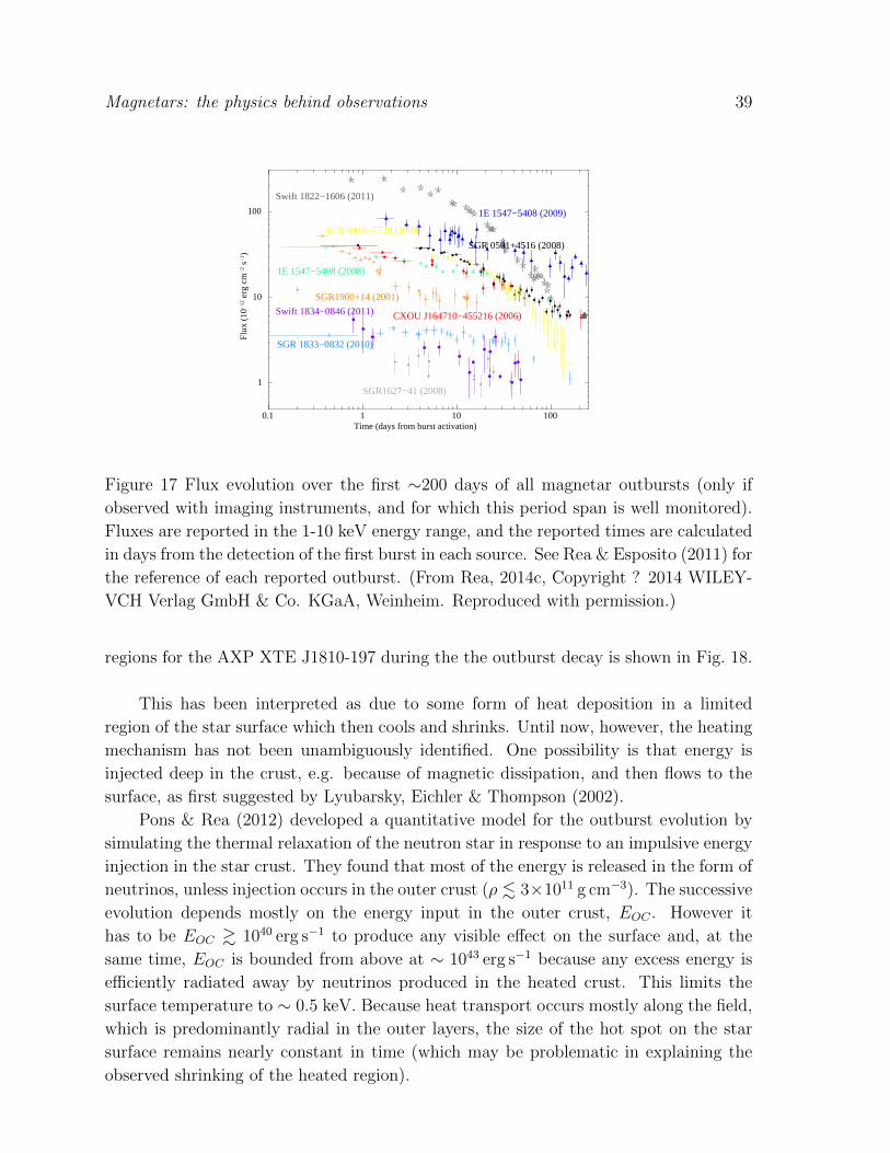
Magnetars: the physics behind observations 39
0.1 1 10 100
1
10
100
Flu
x (1
0−12
erg
cm−
2 s−
1 )
Time (days from burst activation)
SGR1627−41 (2008)
CXOU J164710−455216 (2006)
SGR1900+14 (2001)
SGR 0501+4516 (2008)
1E 1547−5408 (2009)
SGR 0418+5729 (2009)
1E 1547−5408 (2008)
SGR 1833−0832 (2010)
Swift 1834−0846 (2011)
Swift 1822−1606 (2011)
Figure 17 Flux evolution over the first ∼200 days of all magnetar outbursts (only if
observed with imaging instruments, and for which this period span is well monitored).
Fluxes are reported in the 1-10 keV energy range, and the reported times are calculated
in days from the detection of the first burst in each source. See Rea & Esposito (2011) for
the reference of each reported outburst. (From Rea, 2014c, Copyright ? 2014 WILEY-
VCH Verlag GmbH & Co. KGaA, Weinheim. Reproduced with permission.)
regions for the AXP XTE J1810-197 during the the outburst decay is shown in Fig. 18.
This has been interpreted as due to some form of heat deposition in a limited
region of the star surface which then cools and shrinks. Until now, however, the heating
mechanism has not been unambiguously identified. One possibility is that energy is
injected deep in the crust, e.g. because of magnetic dissipation, and then flows to the
surface, as first suggested by Lyubarsky, Eichler & Thompson (2002).
Pons & Rea (2012) developed a quantitative model for the outburst evolution by
simulating the thermal relaxation of the neutron star in response to an impulsive energy
injection in the star crust. They found that most of the energy is released in the form of
neutrinos, unless injection occurs in the outer crust (ρ . 3×10¹¹ g cm−3). The successive
evolution depends mostly on the energy input in the outer crust, EOC . However it
has to be EOC & 1040 erg s−1 to produce any visible effect on the surface and, at the
same time, EOC is bounded from above at ∼ 1043 erg s−1 because any excess energy is
efficiently radiated away by neutrinos produced in the heated crust. This limits the
surface temperature to ∼ 0.5 keV. Because heat transport occurs mostly along the field,
which is predominantly radial in the outer layers, the size of the hot spot on the star
surface remains nearly constant in time (which may be problematic in explaining the
observed shrinking of the heated region).

Magnetars: the physics behind observations 40
Figure 18 The evolution of the spectrum, pulse profile (top panels) and size of the
emitting regions (expressed as fraction of the entire surface, bottom panel) during the
outburst of XTE J1810-179. Results are for the three temperature model (hot cap, warm
corona and cool surface) of Albano et al. (2010); the cold temperature is fixed at 0.15
keV. The adopted spectral model is the superposition of two NTZ’s (see Sec. 3.3.1) at
the hot and warm temperature (adapted from Albano et al., 2010, c©AAS. Reproduced
with permission. A link to the original article via DOI is available in the electronic
version).
Results were successfully applied by Rea et al. (2012a) to fit the outburst decay in
Swift J1822.3-1606 over the entire period covered by their observations, ∼ 250 d after
the first burst that led to the discovery of the source. The case of SGR 0418+5729,
for which a much longer time coverage is available (∼ 1200 d), is, however, much less
conclusive in this respect (Rea et al., 2013a). The calculated flux in the 0.5–10 keV
band systematically overestimates the observed one at later times (& 400 d), when
the luminosity suddenly drops and the hotter blackbody (initially at kT ∼ 0.9 keV)
disappears leaving only a cooler component at ∼ 0.3 keV. A similar effect has been
recently reported in the decay curve of CXOU J1647-4552 around 1000 d (Rodriguez et
al., 2014) and in Swift J1834.9-0846 (Esposito et al., 2013).
Alternatively, heating of the surface layers may be produced by currents flowing in
a twisted magnetosphere as they hit the star. As discussed in §3.1, once implanted by

Magnetars: the physics behind observations 41
crustal displacements, a twist must necessarily decay in order to supply the potential
drop required to accelerate the conduction current (Beloborodov & Thompson, 2007).
The evolution of an untwisting magnetosphere proceeds through the expansion of a
potential region, where ~∇× ~B = 0, which progressively confines the twist to a limited
bundle of current-carrying field lines (the j-bundle), until the twist is completely erased
(Beloborodov, 2009). Fractures, or plastic deformations, most likely affect only a limited
area of the star crust, so the twist is expected to involve only the bundle of field lines
whose footpoints are anchored in the displaced region. As the magnetosphere untwists,
the area covered by the j-bundle shrinks and the luminosity decreases. The rate of
Ohmic dissipation, which depends on the initial twist configuration and on how the
twist angle ∆φ evolves in time (∆φ(t), is not necessary monotonic, the twist may first
decrease and then increase to a maximum value ≈ 1 rad). The simplest model gives
L ≈ 1036
(B
1014 G
)(V
109 V
)(R
106 cm
)2
∆φ sin4 θj−b erg/s (10)
where V is the discharge voltage and θj−b is the angular extension of the j-bundle
on the star’s surface (this is valid for a small polar bundle with maximal twist, see
Beloborodov, 2009). Since heat is unlikely to leak outside the cap at the base of the
j-bundle, the area of the X-ray emitting region is ∼ πR2 sin2 θj−b. A quite definite
prediction of the model is, then, that the luminosity is proportional to the square of the
emitting area throughout outburst evolution (this still holds, at least approximately,
also for more elaborate versions). A spatially-limited twist can also explain the nearly
thermal spectra observed in most transients. If currents fill only a tiny fraction of the
magnetosphere, thermal photons produced in the hot surface regions have only a small
chance of undergoing resonant scattering to populate a high-energy tail.
Beloborodov (2009) found that the model can satisfactorily reproduce the observed
properties of the outburst of XTE J1810-197 for a small twisted region (sin2 θj−b ∼ 0.03)
and large twist angle (∆φ ∼ 1 rad). The application to other transient sources is,
however, not without difficulties. The main problem is that the small size of the
thermally emitting spot, and hence the limited spatial extent of the twist, can make
the luminosity released by Ohmic dissipation too low (especially if the magnetic field
is . 1014 G) to explain the observed flux, like in SGR 0501+4516 (Rea et al., 2009) or
SGR 0418+5729, (Rea et al., 2013a). Moreover, the relation L ∝ A2 does not seem to
be met in other sources (Rodriguez et al., 2014). Different geometries of the j-bundle,
not necessarily involving the polar region, may however ease the energetic requirement.
4.2. Low-field Magnetars
Recently, the commonly accepted picture in according to which the activity in SGRs
and AXPs is necessarily related to a super strong-field (the ‘supercritical B’ paradigm)
has been challenged by the discovery of two fully-fledged magnetars, SGR 0418+5729
and Swift J1822.3–1606, (Rea et al., 2010; Turolla et al., 2011; Rea et al., 2012a;
Livingstone et al., 2011b; Rea et al., 2013a; Scholz et al., 2012) with a dipole magnetic

Magnetars: the physics behind observations 42
field . 1013 G, well within the range of ordinary radio pulsars. A third candididate,
XMM J185246.6+003317, has been reported and awaits further monitoring (Rea et al.,
2014a).
SGR 0418+5729 was discovered on 2009 June 5, thanks to the detection of a couple
of SGR-like bursts (van der Horst et al., 2010). Follow-up observations revealed a
previously unknown bright X-ray source at a flux level of a few times 10−11 erg cm−2 s−1,
pulsating at a period of 9.1 s (van der Horst et al., 2010; Esposito et al., 2010). Based of
ROSAT All-Sky Survey data, the upper limit on the source flux in quiescence is of the
order of 10−12 erg cm−2 s−1. Despite the dense monitoring, no spin-down was detected
during the first ∼ 5 months of observations following the outburst onset. The estimated
upper limit on the period derivative, 1.1× 10⁻¹³ s s−1, translates into an upper limit on
the surface dipole magnetic field strength of 3× 10¹³ G (Esposito et al., 2010).
This made SGR 0418+5729 the magnetar with the lowest dipole magnetic field ever
discovered (for comparison, the previous record holder, the AXP 1E 2259+586, has a
spin-down magnetic field about twice as strong, 6 × 10¹³ G). It took nearly another
3 years of monitoring to finally pinpoint the source spin-down rate from a coherent
timing analysis of all the X-ray data spanning ∼ 1200 days: (4± 1)× 10−15 s s−1,
corresponding to B ∼ 6.1× 10¹² G and to a characteristic age τc = P/(2P ) ' 36 Myrs
(Esposito et al., 2010; Rea et al., 2010, 2013a).
Swift J1822.3-1606 was detected on 2011 July 14, when it emitted several magnetar-
like bursts (Livingstone et al., 2011b; Rea et al., 2012a, and references therein). A few
days after the outburst onset, a new, persistent X-ray source was discovered at a flux
level of ∼ 2 × 10⁻¹⁰ erg cm−2 s−1, pulsating with a period of ∼ 8.4 s. Contrary to the
case of SGR 0418+5729, the source has been already detected in X-rays at a flux level
of ∼ 4 × 10⁻¹⁴ erg cm−2 s−1, although its presence in two ROSAT X-ray catalogues
passed unnoticed (Rea et al., 2012a; Scholz et al., 2012). Swift J1822.3–1606 was
intensely monitored between 2011 July and 2012 August with different X-ray satellites
(Livingstone et al., 2011b; Rea et al., 2012a; Scholz et al., 2012). Phase coherent timing
analyses yield spin-down rates between ∼ 0.7× 10⁻¹³ s s−1 and ∼ 3.1×10⁻¹³ s s−1, and
a dipole magnetic field between 2.4×10¹³ G and 5.1×10¹³ G (Rea et al., 2012a; Scholz et
al., 2012). Despite a precise measurement of P is not available as yet, any of the values
proposed so far makes Swift J1822.3–1606 the magnetar with the second lowest dipole
magnetic field after SGR 0418+5729. Given the low value of the period derivative, the
characteristic age of Swift J1822.3–1606 is quite long, τc ∼ 0.8 Myr, although the source
appears not as old as SGR 0418+5729.
The large characteristic age, the small number of detected bursts with
comparatively low energetics and the low persistent luminosity in quiescence have been
taken as suggestive that these are “old magnetars” approaching the end of their active
life, in which the magnetic field has experienced substantial decay (Esposito et al., 2010;
Rea et al., 2010; Turolla et al., 2011). A key question is if, and to what extent, the
present (internal) magnetic field is still strong enough to stress the crust and produce
bursts/outbursts. Indeed, Turolla et al. (2011) and Rea et al. (2012a) have shown

Magnetars: the physics behind observations 43
Figure 19 From top left to bottom right: time evolution of P , P , LX and Bp for
Swift J1822.03–1606. The dashed vertical line marks the estimated age of the source;
the gray strips in the first two panels show the observed values of P and P with their
uncertainties. The model is for Btor(t = 0) = 5×10¹⁵ G (from Rea et al., 2012a, c©AAS.
Reproduced with permission. A link to the original article via DOI is available in the
electronic version ).
that the magneto-thermal evolution (Pons et al., 2009; Vigano et al., 2013, see §2) of
an initially ultra-magnetized neutron star, Bp(t = 0) ∼ 2 × 10¹⁴ G, can reproduce
the observed P , P , Bp and LX in SGR 0418+5729 and Swift J1822.3–1606, for an age
∼ 1 Myr and ∼ 0.5 Myr, respectively, provided that the initial internal toroidal field
Btor(t = 0) is high enough∗. The evolution of the period, period derivative, dipole
B-field and luminosity for Swift J1822.03–1606 is shown in Fig. 19. The fact that the
characteristic age (assuming a constant B) in these two sources is largely in excess
of that derived from magneto-thermal evolution reflects a quite general property of
magnetar sources, for which characteristic ages are longer than those derived using
other estimators.
∗ More recent calculations of magneto-thermal evolution including the Hall drift actually show that a
strong toroidal component develops regardless of the initial topology the the magnetic field (Vigano et
al., 2013).

Magnetars: the physics behind observations 44
According to the calculations by Perna & Pons (2011), who modeled the evolution
of the internal magnetic stresses in a magnetar, the occurrence of crustal fractures (and
hence of bursts/outbursts) can extend to late phases (≈ 105–106 yr). Both the energetics
and the recurrence time of the events evolve as the star ages and depend on the initial
field. The models which successfully reproduce the properties of the two low-field sources
imply that the two low-B magnetars could become burst-active despite their age, with
an expected (current) event rate of ≈ 0.01–0.1 yr−1.
Quite recently, Tiengo et al. (2013) reported the discovery of a phase-variable
absorption feature in the X-ray spectrum of SGR 0418+5729. The feature is best
detected in a 67 ks XMM observation performed on 2009 August 12, when the source
flux was still high (5 × 10⁻¹² erg cm−2 s−1 in the 2–10 keV band) but is also visible in
the RXTE and Swift data collected in the first two months after the outburst onset.
The line energy is in the range ∼ 1–5 keV, in XMM data, and changes sharply with
rotational phase, by a factor of ∼ 5 in one-tenth of a cycle (see Fig. 20). These seem
to favour an interpretation in terms of a cyclotron line. If protons, e.g. contained in a
rising flux tube close to the surface, are responsible for the line, the local value of the
magnetic field within the baryon-loaded structure is close to 1015 G. SGR 0418+5729
would then be, at the same time, the magnetar with the lowest dipole field and the
neutron star with the largest (small-scale) field ever measured.
4.3. Transient Radio Emission
For a long time SGRs and AXPs were thought to be with no exceptions radio quiet,
to the point that the lack of (pulsed) radio emission was often quoted as one of their
defining properties. In fact, an expanding radio nebula was detected in the aftermath
of the Giant Flares from SGR 1806-20 (Gaensler et al., 2005b; Cameron et al., 2005)
and SGR 1900+14 (Frail, Kulkarni & Bloom, 1999), but this originated in the shocked
material around the neutron star and not from the star magnetosphere.
The first detection of pulsed radio emission from a magnetar came, rather
unexpectedly, from the archetypal transient XTE J1810-197 (Camilo et al., 2006),
opening a new window in the study of magnetars. For many months, XTE J1810-197
was the brightest radio pulsar in the Galaxy at frequencies above 20 GHz, exhibiting
a strong variability in both the radio flux and the pulse shape on different timescales.
The radio emission likely began about a year after the onset of the X-ray outburst and
lasted a few years (Camilo et al., 2006, 2007a; Lazaridis et al., 2008; Serylak et al., 2009).
Pulsed radio emission was then discovered from the AXP 1E 1547-5408 (Camilo et al.,
2007b). This source has shown three X-ray outbursts in the past 5 years. Radio emission
was observed in the interval between the last two events, during which it declined, to
rise again in coincidence with the last outburst, although there was a delay of a few
days between the onset of the X-ray outburst and the radio activity (Camilo et al.,
2009; Burgay et al., 2009). Another possibility is that the radio emission was blinking,
in a way uncorrelated with the start of the X-ray outburst. PSR 1622-4950 (Levin et

Magnetars: the physics behind observations 45
0.5 0.6 0.7 0.8 0.9 1 1.1 1.2 1.3 1.4 1.5
0 0.2 0.4 0.6 0.8 1 1.2 1.4 1.6 1.8 2
1000
080
0060
0040
0020
00
Phase
Ener
gy (e
V)
Figure 20 The phase-dependent spectral feature in the EPIC data of SGR 0418+5729.
Normalized energy versus phase image obtained by binning the EPIC source counts into
100 phase bins and 100-eV-wide energy channels and dividing these values first by the
average number of counts in the same energy bin (corresponding to the phase-averaged
energy spectrum) and then by the relative 0.310 keV count rate in the same phase
interval (corresponding to the pulse profile normalized to the average count rate). The
red line shows (for only one of the two displayed cycles) the results of a simple proton
cyclotron model consisting of a baryon-loaded plasma loop emerging from the surface
of a magnetar and intercepting the X-ray radiation from a small hot spot (from Tiengo
et al., 2013, the authors acknowledge Nature Publishing Group for reproduction).
al., 2010) was the first (and so far the only one) magnetar which was discovered thanks
to observations in the radio band. New and archival X-ray observations have shown
that the source is likely a transient magnetar which underwent an outburst in 2007
(before the first available Chandra observation). The X-ray flux is still declining as the
source approaches quiescence (Anderson et al., 2012). Finally, pulsed radio emission
has been detected from the recently discovered magnetar in the Galactic Centre, SGR
J1745-2900 (Rea et al., 2013b; Eatough et al., 2013; Shannon & Johnston, 2013; Kaspi
et al., 2014). The source entered an outburst phase with the emission of a single
burst on April 24 2013. The radio activity switched on 4-5 days after the outburst
onset with similar properties to those of the other two magnetars detected at radio
wavelengths. Despite intensive searches, pulsed radio emission was not found in other
magnetar sources (Burgay et al., 2006; Crawford et al., 2007; Lazarus et al., 2011).
Although the sample is quite limited, a number of common features in the radio

Magnetars: the physics behind observations 46
emission from magnetars have started to emerge: i) association with X-ray outbursts,
ii) the radio flux decays together with the X-ray flux but its onset is delayed, iii) marked
variability in the radio band, and iv) flat radio spectrum. All these properties are much
at variance with those of ordinary radio pulsars (including the high-B PSRs). Rea et
al. (2012b) have shown that radio-loud magnetars are characterized by LX < E in
quiescence, much as ordinary radio pulsars, while the X-ray luminosity always exceeds
the rotational energy loss rate in radio-silent magnetars. In fact, as indicated by Ho
(2013), this property seems to be characteristic also of other classes of neutron stars,
although the inverse is not true: not all sources with LX < E emits in radio. SGR
J1745-2900, which was not included in the original sample considered by Rea et al.
(2012b), further confirms this picture, having E ∼ 5×1033 erg s−1 and LX . 1032 erg s−1
in quiescence (Rea et al., 2013b). This seems to point to a common origin for the
radio emission in PSRs and in transient magnetars. In magnetars with LX/E < 1
particle acceleration and the subsequent ignition of the cascade process could proceed
as in normal pulsars, and their radio emission might basically follow the same rules,
with rotational energy driving pair creation through a cascade. The largely different
radio properties between the two groups might result from the presence of a substantial
toroidal component in the magnetosphere of the magnetars, contrary to the nearly
dipolar field of PSRs. The influence of the large charge density required to support
the non-potential field may also act in quenching the radio emission in the brightest
magnetars with LX/E > 1 (Thompson, 2008a,b), although this latter interpretation
is hard to be reconciled with the fact that, in at least few sources (SGR J1745-2900,
XTE J1810-197 and possibly also in 1E 1547-5408 during the 2009 outburst), radio
emission was seen while the source was bright with LX > E.
5. Magnetar bursts
5.1. Burst phenomenology
One of the hallmarks of magnetars is the emission of repeated soft gamma-ray bursts,
and this feature played a key role in their discovery (for a nice review of the history of the
field, see Woods & Thompson, 2006). Bursts have now been observed from 18 sources
whose spin has also been measured (confirming that they are indeed neutron stars) ].
Magnetars emit bursts in the few keV to few hundred keV energy band (hard X-ray/soft
gamma-ray). As mentioned in the Introduction, magnetar bursts are typically grouped
into three classes defined primarily by energy released and their duration: short bursts
(with energies up to 1041 erg), intermediate flares (energies in the range 1041−1043 erg),
and giant flares (energies in the range 1044−1046 erg, see Fig. 21 for example lightcurves
from the different types of burst).
Bursting activity is highly variable. Sources can experience long periods of apparent
quiescence (when bursting, if it occurs, is in the form of low luminosity bursts below
] See the Amsterdam Magnetar Burst Library, http://staff.fnwi.uva.nl/a.l.watts/magnetar/mb.html

Magnetars: the physics behind observations 47
Figure 21 Examples of different types of magnetar bursts. Top left: Short bursts from
SGR 0501+4516 recorded by Fermi/GBM (from Huppenkothen et al., 2013). Top right:
Burst storm from 1E 1547.0-5408 recorded by Fermi/GBM, with inset showing the
overall enhancement in emission during this event(from Kaneko et al., 2010). Lower left:
Intermediate burst from SGR 1900+14 recorded by RXTE (from Ibrahim et al., 2001).
Lower right: Giant flare from SGR 1900+14 recorded by Ulysses, upper panel showing
OTTB spectral temperature (from Hurley et al., 1999b). The first three panels are
c©AAS, reproduced with permission. A link to the original articles via DOI is available
in the electronic version. The last panel is reprinted by permission from Macmillan
Publishers Ltd: Nature, c©1999. The authors acknowledge Nature Publishing Group
for allowing reproduction.
the detection threshold of our current generation of space telescopes - note also that
there have been gaps in gamma–ray telescope coverage since the discovery of magnetars,
due to the lack of suitable telescopes, and that sky coverage even now is never 100%),
sporadic and highly occasional bursting, or periods of high burst activity. At their most
dramatic, these can climax in burst storms (when several hundreds of bursts can be
emitted over just a few hours), or rare giant flares (Fig. 21). During such outburst
periods there may also be changes in the overall emission (luminosity, pulsed flux and
spectrum, see Rea & Esposito 2011 for an observational review, and Pons & Rea 2012

Magnetars: the physics behind observations 48
for a recent theoretical study) and the timing behaviour (spin-down rate and glitching,
see for example Woods et al. 2001, 2002, 2003, 2007; Dib & Kaspi 2014). There is
no clear dependence of short/intermediate bursting activity on the dipolar magnetic
field strength of the source. The most energetic giant flares come from three sources
whose inferred dipole fields are amongst the highest (a few times 1014 G up to ∼ 1015
G). However bursts have also been seen from sources with fields apparently below the
quantum critical limit, such as Swift J1822.3-1606 with a field ≈ 1.35× 10¹³ G (Scholz,
Kaspi & Cumming, 2014) and SGR 0418+5729 with field 6×10¹² G (Rea et al., 2010)††.
5.1.1. Short bursts Short bursts are the most common, with fluences in the range
10−11 − 10−5 erg/cm2/s, which for the assumed distances implies isotropic energies in
the range 1036 − 1041 erg (Gogus et al., 1999, 2000; Woods et al., 1999b; Gavriil, Kaspi
& Woods, 2004; Kumar, Ibrahim & Safi-Harb, 2010; Scholz & Kaspi, 2011; Lin et al.,
2013). Peak luminosities are in the range 1036− 1042 erg/s, extending to well above the
standard Eddington luminosity of ≈ 2×1038 erg/s for a non-magnetic neutron star. The
lowest luminosity bursts recorded are at the sensitivity limit of our current generation
of detectors. For sources that have shown sufficient numbers of bursts for meaningful
statistical analysis (SGR 1806-20, SGR 1900+14, SGR 1627-41, 1E 2259+286, SGR
0501+5416 and 1E 1547.0-5408), burst fluences are distributed as a power law, dN =
E−γ dE with γ ∼ 1.4 − 2.0 (Cheng et al., 1996; Aptekar et al., 2001; Woods et al.,
1999b; Gogus et al., 1999, 2000, 2001; Gavriil, Kaspi & Woods, 2004; Kumar, Ibrahim
& Safi-Harb, 2010; Savchenko et al., 2010; Lin et al., 2011a; Scholz & Kaspi, 2011;
Prieskorn & Kaaret, 2012; van der Horst et al., 2012). Burst durations are ∼ 0.01− 1s
and are distributed lognormally with a peak at ∼ 0.1s, less than the rotational period
of the star. Duration is correlated with fluence. Bursts from the sources that have
shown insufficient events for full statistical analysis are consistent with this picture.
Lightcurves are extremely variable in shape: the rise is in general faster than the decay
(Gogus et al., 2001; Gavriil, Kaspi & Woods, 2004), but bursts can be multi-peaked, and
no simple phenomenological model has yet been found that would fit the morphologies of
the different burst lightcurves. Some short bursts (classified according to their fluence)
from five sources have extended faint tails of ∼ 100 − 1000 s in duration, leading to
an overall energy release that can exceed that of the original spike (Woods et al., 2005;
Gavriil, Kaspi & Woods, 2004, 2002, 2006; Dib, Kaspi & Gavriil, 2009; An et al., 2014a;
Gavriil, Dib & Kaspi, 2011; Mereghetti et al., 2009; Savchenko et al., 2010; Scholz &
Kaspi, 2011). The tails appear to be pulsed at the rotational frequency.
From the sources with large samples, wait times (for bursts above the detection
threshold, in periods of continuous telescope coverage†) form a lognormal distribution
††Although note that the dipole field strength as estimated from spin down provides only a lower limit
on the magnetic field strength, and there are no constraints on the strength of either higher order
poloidal components or toroidal components.† The recent detection of short bursts from 1E 1547.0-5408, in the VLF radio band due to the
ionospheric disturbance that occurs as the incident gamma-rays ionize the Earth’s atmosphere opens

Magnetars: the physics behind observations 49
with a peak at ∼ 100s. During the active period of SGR 1900+14 in 1998, for example,
Gogus et al. (1999) found wait times ranging from less than 1s to more than 1000s‡,and far longer wait times are clearly possible: SGR 1900+14, for example, has also had
quiescent periods ∼ years in duration. The shortest wait times observed are comparable
to the durations of individual bursts, such that the distinction between single bursts
and multi-peaked events is not clear. There appears to be no correlation between
burst intensity and wait time to the following burst (Laros et al., 1987; Gogus et al.,
2000; Gavriil, Kaspi & Woods, 2004; Savchenko et al., 2010). Of particular note in the
discussion of wait times are burst storms, periods of unusually high short burst activity
(which may include some intermediate flares), in which tens to hundreds of bursts occur
over only a few hours on top of an overall rise in emission that can be strongly pulsed
at the rotational phase (see for example Hurley et al., 1999a; Israel et al., 2008; Gavriil,
Kaspi & Woods, 2004; Mereghetti et al., 2009; Kaneko et al., 2010; Savchenko et al.,
2010, for the cases SGR 1900+14, 1E 2259+286, and 1E 1547.0-5408). There have also
been efforts to determine whether the occurrence of bursts correlates with rotational
phase: here the evidence is mixed. For 1E 1048.1-5937, 1E 2259+286 and XTE J1810-
197 bursts do seem to occur preferentially at rotational pulse maxima (Gavriil, Kaspi
& Woods, 2002, 2004; Woods et al., 2005). However for SGR 1806-20, SGR 1900+14,
SGR 1627-41, 4U 0142+61 and 1E 1547.0-5408 no such correlation is found (Palmer,
1999, 2002; Woods et al., 1999b; Gavriil, Dib & Kaspi, 2011; Savchenko et al., 2010;
Scholz & Kaspi, 2011; Lin et al., 2012a).
5.1.2. Intermediate flares Intermediate flares, with (isotropic) energies in the range
∼ 1041−1043 erg, and peak luminosities that exceed the non-magnetic Eddington limit,
have been seen from SGR 1627-41, SGR 1900+14, SGR 1806-20, and 1E 1547.0-5408.
The primary bursts appear to be brighter and slightly longer (durations ∼ 0.5s up to
a few s) versions of the short bursts. Morphologies, however, are varied. Some have a
clear decay and an abrupt end (Mazets et al., 1999a,b; Olive et al., 2004; Israel et al.,
2008). In others the initial burst is followed by a extended decaying tail that can last for
up to several thousand seconds, but contains less than ∼ 2 % of the energy released in
the initial peak (Ibrahim et al., 2001; Lenters et al., 2003; Esposito et al., 2007b; Gogus
et al., 2011b). The tails are pulsed at the rotational period of the star: in some cases
the pulsed amplitude rises dramatically (Ibrahim et al., 2001; Lenters et al., 2003), as
seen during some burst storms (Kaneko et al., 2010); whilst in others no change is seen
(Gogus et al., 2011b). The pulsations appear for the most part to be phase-aligned with
the pre-burst pulsations, but there are some occasional exceptions (Guidorzi et al., 2004;
Gogus et al., 2011b). There has also been one burst with a decaying pulsed tail, where
the sharp initial burst peak appears to be absent, leading to a rather slow rise time
∼ 10s (Kouveliotou et al., 2001; Guidorzi et al., 2004). Intermediate flares sometimes
up the possibility of using the VLF band to obtain a more complete coverage of the waiting time
distribution with being dependent on sky coverage of space telescopes (Tanaka et al., 2010).‡ The longest wait times in this study were set by the length of the observing window.

Magnetars: the physics behind observations 50
have short precursors (Ibrahim et al., 2001; Gogus et al., 2011b), and during some events
short bursts are seen during the extended tail (Ibrahim et al., 2001; Lenters et al., 2003;
Gogus et al., 2011b).
5.1.3. Giant flares The most energetic bursts, the giant flares, are extremely rare. Only
three have ever been seen, in 1979, 1998 and 2004, each from a different magnetar (SGR
0526-66, SGR 1900+14, and SGR 1806-20). The total energy released, if the emission
is isotropic and assuming reliable estimates of distance, is in the range 1044 − 1047 erg
(Fenimore et al., 1996; Feroci et al., 2001; Palmer et al., 2005). The overall properties
of the three giant flares are, despite the differences in energy, very similar (in marked
contrast with the heterogeneity of the intermediate flares). They have a very bright
initial peak, followed by an extended decaying tail with a duration of several hundred
seconds that is strongly pulsed at the rotational frequency of the star† (see e.g. Mazets
et al., 1979a; Hurley et al., 1999b; Hurley et al., 2005).
The initial peaks, which can have rise times as short as ∼ 1 ms, last ∼ 0.1 − 1
s and are very hard. Luminosities reach up to 1047 erg/s (Hurley et al., 2005), which
causes substantial dead time and pile up effects in space telescopes. This renders reliable
spectral modelling very difficult, however the spectrum is very hard, with emission being
detected up to 2 MeV (Mazets et al., 1979a; Hurley et al., 1999b). The initial peaks are
strongly variable, on timescales as short as a few ms (Barat et al., 1979; Hurley et al.,
1999b; Terasawa et al., 2005; Schwartz et al., 2005). Both the SGR 1900+14 and SGR
1806-20 giant flares were observed to have precursors†. For SGR 1900+14 the precursor
resembled a normal short burst, and occurred < 1 s before the giant flare (Mazets et
al., 1999c). For SGR 1806-20 the precursor was flat-topped, with an energy release that
puts it in the intermediate flare class, and occurred 142 s prior to the giant flare (Hurley
et al., 2005). A discussion of whether the apparent precursors are in fact genuinely
causally connected to the giant flares was presented by Gill & Heyl (2010).
The energies emitted in the tails of the three giant flares have been similar (∼ 1044
erg). This is 1− 2% of the energy released in the initial peak of the 2004 giant flare: for
the two earlier giant flares the energies released in initial peak and tail were comparable.
The overall envelope of the tails (averaged over rotational phase) decays smoothly as a
power law, coming to an abrupt end after several hundred seconds. The pulsations in
the SGR 0526-66 giant flare tail were seen immediately after the initial peak; for the
other two giant flares they appeared only a few tens of seconds later. Pulse profiles
can evolve during the tails, in the case of SGR 1900+14 simplifying quite dramatically
(Feroci et al., 2001), with evolution being much more minimal for SGR 1806-20 (Palmer
† Note that none of the giant flares were caught during pointed observations: they are so rare but so
bright that most are seen off-axis. This means that the sensitivity to late time weak emission is much
less than for some of the intermediate flares, which were observed during pointed observations. One
should bear this in mind when comparing the apparent durations.† A precursor with the properties observed for SGR 1900+14 giant flare would not have been detectable
for the SGR 0526-66 giant flare given the instrumentation at the time (Gill & Heyl, 2010).

Magnetars: the physics behind observations 51
et al., 2005; Mereghetti et al., 2005c; Boggs et al., 2007; Xing & Yu, 2011). The giant
flares are so strong that they have a detectable effect on the Earth’s electromagnetic
field (Mandea & Balasis, 2006) and ionosphere (Inan et al., 1999, 2007; Tanaka et al.,
2008), with even the rotational pulsations being clearly visible, and this has been used
to put lower limits on the strength of low energy (< 10 keV) emission from the burst
(unaffected by satellite dead time issues).
Radio afterglows were detected after both the SGR 1900+14 and SGR 1806-20
giant flares (Frail, Kulkarni & Bloom, 1999; Cameron et al., 2005; Gaensler et al., 2005b;
Gelfand et al., 2005; Taylor et al., 2005; Fender et al., 2006). The amount of energy in
the radio afterglow is much less than that emitted in the gamma-rays. This is different
from what is observed in gamma ray bursts, where the ratio between the two types
of emission is of order unity, such that the lower energy and longer duration emission
is associated with re-processing of the gamma-ray energy by the surrounding material.
The radio afterglow from the magnetar giant flares is linearly polarized, implying that
it is caused by electron synchrotron emission, and is observed to expand over time. Its
generation requires an ejection of relativistic particles and magnetic fields (in the form
of a “plasmon”, which expands and cools) by the burst process (see Section 5.3).
5.2. Burst trigger mechanisms
Rapid magnetic field reconfiguration is assumed to be an integral part of the bursts: as
we will discuss in Sec. 5.3, the gamma-ray emission is assumed to come from particles
accelerated by rapid field change. Thus slow magnetic evolution builds up stresses in
the system, some of which are released catastrophically in bursts, which must either be
driven by or result in rapid magnetic field reconfiguration. However the precise trigger
mechanism, and the role of the magnetic field within it (if any), remains unclear. Three
main locations (and associated families of instabilities) have been considered for the
trigger mechanism: below we review each in turn.
The first option, as suggested by Thompson & Duncan (1995), is that the magnetic
field evolves into an unstable configuration within the liquid core of the star (Markey,
1973; Wright, 1973; Tayler, 1973; Flowers & Ruderman, 1977), which is then susceptible
to a large-scale magnetohydrodynamical instability (Lander & Jones, 2011a; Ciolfi et al.,
2011; Kiuchi, Yoshida & Shibata, 2011; Ciolfi & Rezzolla, 2012). This would develop on
the Alfven crossing time of the core, which is ∼ 0.1s for a 1015 G interior field (τ ∼ R/vA,
where the Alfven speed vA is given in Equation 16 later in this paper) and hence broadly
compatible with the durations of both the normal bursts and the initial peaks of the
giant flares.
Whether such an unstable state could develop is open to question, since if the core
is superconducting, the high conductivity should facilitate swift reconfiguration and
hence prevent the formation of such an unstable state. However the configuration could
be stabilized by currents in the crust, or superconductivity may be suppressed if the
core field exceeds ∼ 1016G. Such rapid internal magnetic reconfiguration would inject

Magnetars: the physics behind observations 52
an Alfven pulse into the magnetosphere that would then generate the observed burst
emission. The energy available to power the burst in this scenario, since it originates in
the core, is more than sufficient to power even a giant flare. Some internal heat release
may also be expected due to dissipation in core and crust as the instability proceeds.
The second option is that the decay of the core field places magnetic stresses on
the solid crust of the star (an ionic lattice to which the field in the crust is locked).
The crust can deform elastically to accommodate this up to a certain point, then
ruptures catastrophically once its breaking strain is exceeded (Thompson & Duncan,
1995; Thompson & Duncan, 2001). The stored energy released in this scenario would
come from the crust and possibly also the core: although initially it was thought that the
crust alone could not store enough elastic energy to power the giant flares (Thompson
& Duncan, 1995), the latest molecular dynamics simulations predict a higher breaking
strain, indicating that this may be feasible after all (Horowitz & Kadau, 2009; Hoffman
& Heyl, 2012). Studies are now underway that aim to determine how and where stresses
would build up in the crust as a result of core field evolution, the goal being to determine
how often, and where (location including depth) the crust is most likely to fail (Perna
& Pons, 2011; Pons & Perna, 2011; Beloborodov & Levin, 2014; Lander et al., 2015).
Recent calculations by Lander et al. (2015) of the strain induced in a crust by a changing
magnetic field configuration find a characteristic burst energy
E
1045erg≈ 0.25
( σmax
0.001
)( d
Rc
)2(l
2πR
)(11)
where σmax is the breaking strain of the crust (which could be as high as 0.1; Horowitz
& Kadau, 2009), d is the depth at which the crust ruptures, Rc the crust thickness, R is
the star radius, and l the rupture length. The characteristic local field strength related
to crust breaking (from the same study) is given by
Bbreak = 2.4× 10¹⁴G( σmax
0.001
)1/2
. (12)
When the crust does rupture it must do so by rapid plastic deformation, not via
brittle fracture, due to the impossibility of opening up voids under the conditions of
extreme pressure that pervade in neutron star crusts (Jones, 2003). The role of the
magnetic field during crust rupture however is not clear: Levin & Lyutikov (2012) have
argued that under some circumstances the field deformation induced by an incipient
rupture may act as a brake on its propagation. Shear wave timescales (which control
the timescale on which the crust ruptures, τ ∼ πR/vs, where the shear speed vs is
given by Equation 15 later in this paper) are compatible with those observed in bursts
and flares (see for example Schwartz et al., 2005), injecting an Alfven pulse into the
magnetosphere. However the transfer of energy into the external magnetosphere may
be slowed by a large impedance mismatch at the crust-magnetosphere boundary (Link,
2014). Crustal rupture would most likely lead to local heating as well.
The final possibility is that the core and crust evolve smoothly, and that stress builds
up instead in the magnetosphere. Stress release is then envisaged as taking place via

Magnetars: the physics behind observations 53
a plasma instability involving spontaneous magnetic reconnection (see Uzdensky, 2011,
for a review). A number of studies have looked at how the external magnetosphere
might respond to the expulsion of magnetic helicity due to the decaying core field, and
have found that the development of unstable configurations with strong magnetic shear,
that might be prone to reconnection instabilities, is feasible (Thompson, Lyutikov &
Kulkarni, 2002; Beloborodov, 2009; Parfrey, Beloborodov & Hui, 2012; Parfrey et al.,
2013). The resulting explosive reconnection event would progress on the Alfven crossing
time in the magnetosphere, which is . 0.01 s (since in the magnetosphere vA ∼ c),
and the energy that can be released is more than sufficient to power even the giant
flares. Specific instabilities that have been considered primarily for the giant flares
(driven by earlier concerns about the ability of crust ruptures to release enough energy)
are the relativistic tearing mode (Lyutikov, 2003, 2006; Komissarov et al., 2007) and
collisionless Hall reconnection mediated by emission from precursor bursts (Gill & Heyl,
2010), the precursors presumably being triggered in this scenario by another mechanism.
Similarities between the giant flares and reconnection driven coronal mass and flux tube
ejection events in solar physics have also been explored in some depth (Masada et al.,
2010; Yu, 2011, 2012; Yu & Huang, 2013; Huang & Yu, 2014a,b; Meng et al., 2014).
Instabilities may also arise from the interaction of MHD waves with the vacuum in fields
above the quantum critical limit (where QED effects are important, Heyl & Hernquist,
2005). All of these mechanisms would lead directly to particle acceleration and radiation
in the magnetosphere, with possible crustal heating via particles impacting the surface.
At present it is by no means clear which of the various mechanisms are in operation,
and given the diversity of burst properties (Sec. 5.1) more than one may be in operation.
Timescales, as discussed above, appear to be roughly compatible with either burst rise
times or durations (assuming that the emission process timescales reflect those of the
trigger mechanism). Moreover both starquakes and magnetospheric reconnection could
in principle explain the power law distribution of fluences (which is often taken as
evidence for Self-Organised Criticality, see for example Aschwanden et al., 2014). Serious
efforts are now being made to simulate the build up of stress and the development of
instabilities, but in order to allow meaningful tests of the data, consideration must be
given to how these various triggers connect to the emission that we see. We discuss this
in the next section (Sec. 5.3).
5.3. Burst emission processes
5.3.1. Sources of emission Magnetar bursts are complex, with varied spectra and
morphologies. The emission process for all bursts is generally assumed to be started by
rapid rearrangement of the magnetic field (resulting from one of the trigger mechanisms
discussed in Sec. 5.2), possibly involving either induced or spontaneous magnetic
reconnection. This accelerates charged particles with ensuing gamma-ray emission,
since the rapid acceleration of electrons in a strong curved field leads to a cascade of pair
creation and gamma-rays (Sturrock, Harding & Daugherty, 1989). To obtain the hardest

Magnetars: the physics behind observations 54
emission, there must be very low contamination by baryonic material (since scattering
would lead to softening). Fully self-consistent models of the emission resulting from the
various proposed trigger mechanisms do not yet exist. Despite this, the rise timescale
of the gamma-ray emission has frequently been used as a key piece of evidence to argue
for a particular trigger mechanism, as discussed in the previous section. However it is
not clear that this is warranted: details of the gamma-ray emission process may in fact
completely obscure the timescales associated with the original trigger mechanism (see
for example Hoshino & Lyubarsky, 2012).
To obtain the radio afterglow seen in the giant flares, it is necessary to postulate
the ejection of a plasmoid of magnetic fields and trapped shocked plasma, that gradually
cools (Sec. 5.1). Such plasmoid ejection is a natural and expected consequence of a large-
scale reconnection event in the magnetosphere (see Sec. 5.2 and for example Lyutikov,
2006).
The initial spike of magnetar flares may also lead to radio emission (explored for
example in Lyutikov, 2002). More recently it has been suggested that the interaction
between strongly magnetized relativistic ejecta (expelled by the initial spike of giant
flares) and the surrounding wind nebula might be responsible for extragalactic Fast
Radio Bursts (Popov & Postnov, 2007, 2013; Thornton et al., 2013; Lyubarsky, 2014).
At present this remains speculative.
If the local energy generation rate is high enough, as explained above, it will lead to
copious production of electron-positron pairs and gamma-rays. If this occurs in a closed
field line region, where the charged pairs cannot cross magnetic field lines, they become
trapped. As density increases, so does optical thickness, trapping the photons as well
and leading to rapid thermalization (Thompson & Duncan, 1995). The field necessary
to confine the plasma can be estimated by requiring that magnetic pressure exceed the
pressure of the radiation and the pairs at the outer boundary of the fireball, yielding
Bdipole > 2× 10¹⁴
(Efireball
1044 erg
)1/2(∆R
10 km
)−3/2(1 + ∆R/R
2
)3
G (13)
(Thompson & Duncan, 2001), where ∆R is the characteristic size of the fireball and R
the neutron star radius.
Such a trapped pair plasma fireball would then cool and contract due to radiative
diffusion from a thin surface layer, with the bulk of the radiation leakage occurring close
to the stellar surface since this is where the field is strongest and scattering the most
suppressed. The opacity at the surface will be dominated by the electron-ion plasma
ablated from the neutron star surface (especially if the emergent flux is close to the
magnetic Eddington limit) which form the photosphere. This trapping would prolong
the emission from the burst by acting as a reservoir for the energy. Fireball formation is
not exclusively linked to any one trigger mechanism (Thompson & Duncan, 1995; Heyl
& Hernquist, 2005).
The fireball model has been very successful at explaining the later decaying tail
phase of giant flares (Thompson & Duncan, 2001). A cooling fireball trapped on

Magnetars: the physics behind observations 55
closed field lines should have a luminosity L whose time-dependence is described by
the following function
L(t) = L(0)
[1− t
τevap
]a/(1−a)
(14)
where the cooling luminosity is assumed to vary as a power of the remaining fireball
energy, L ∝ Ea (Thompson & Duncan, 2001). This proves to be a good fit to giant flare
tail data, with τevap of order a few hundred seconds, and a value of a that is close to that
expected for a spherical fireball of uniform temperature (Feroci et al., 2001). Spectral
fitting indicates that the emitting area falls while the temperature of the radiation
remains roughly constant at the level expected for the photosphere of a trapped fireball
in a magnetic field in excess of the quantum critical field (Thompson & Duncan, 1995;
Feroci et al., 2001). The observed photospheric temperature (∼ 20 − 30 keV) is lower
than the inferred temperature in the core of the fireball, which is ∼ 100 keV (Thompson
& Duncan, 1995; Thompson & Duncan, 2001). Thompson & Duncan (1995) argue
that this is an intrinsic property of the way various processes act to preserve thermal
equilibrium in the fireball, and the way that radiation gradually escapes. However
other processes such as photon splitting as the emitted radiation propagates through
the strong magnetic field may also be important (Baring, 1995). The beaming of
radiation as it leaks from the base of the fireball and streams along field lines provides a
simple explanation for the strong rotational pulses seen in the giant flare tails (Fig. 22).
Whether fireballs form in the smaller bursts is still not clear (energy release may not
occur at a fast enough rate (Gogus et al., 2001), although the similarity of the spectra
of the short bursts to the spectra in the tails of the giant flares suggests that there may
be a link.
Some of the energy released during the burst is likely to excite vibrations, either of
the star (crust/core, see Sec. 5.4) or in the form of Alfven waves in the magnetosphere.
This too can act as a store for energy that is then radiated on longer timescales. If the
vibration rate is slow enough, this can act as a source of ongoing excitation that forms
an extended pair corona (that obscures and scatters the radiation from the trapped
fireball) from which the radiation emerges isotropically (Feroci et al., 2001; Thompson
& Duncan, 2001). The presence of such an extended pair corona has been invoked to
explain the smooth emission immediately after the peak of the giant flares, which then
clears over 30-40 s to reveal the strongly beamed rotational pulse emanating from the
trapped fireball beneath (Feroci et al., 2001).
A burst may also have a thermal component of emission that is produced by residual
heat of crust rupturing (Lyubarsky, Eichler & Thompson, 2002; Kouveliotou et al.,
2003), extreme heating and possible melting of the crust immediately underneath a
trapped fireball (Thompson & Duncan, 1995), or bombardment of the stellar surface
by magnetospheric particles (Lyutikov, 2006; Beloborodov, 2009). Such thermal
components, particularly deep crustal heating, are one possible explanation for the
presence of both the additional pulsed components seen after some bursts (short and

Magnetars: the physics behind observations 56
10
1
0.1
0.01 1 10 100
F
εI (keV)
Cyclotron absorption
Photon splitting
Figure 22 Left: Figure from Thompson & Duncan (2001), to illustrate how radiation
escapes from a trapped photon-pair plasma fireball. Scattering opacities are strongly
polarization dependent, with most radiation escaping from the fireball in the E-mode.
This radiation is then collimated along open magnetic field lines (due to the magnetic
field dependence of the scattering opacties), forming a beam that is then modulated
by the star’s rotation to give rise to a rotational pulse (from Thompson & Duncan,
2001, c©AAS. Reproduced with permission. A link to the original article via DOI is
available in the electronic version). Right: Figure from Lyubarsky (2002) showing how
the photospheric spectrum from a fireball with temperature 15keV (dashed line) would
be modified by various high field radiation processes: cyclotron absorption, for a 6×10¹⁴
G field, and photon splitting (from Lyubarsky, 2002, with OUP permission).
intermediate) - as a localised hotspot - and the must longer decaying afterglows seen
after burst active periods, intermediate flares and giant flares (Kouveliotou et al., 2003;
Feroci et al., 2003).
The location of the emitting regions is further complicated by the fact that the
luminosity of the bright bursts may exceed the relevant Eddington limit, leading to
photospheric expansion and ejection of material as radiation pressure overwhelms the
gravitational force (see for example Thompson & Duncan, 1995; Watts et al., 2010).
Magnetar bursts can easily exceed the non-magnetic Eddington limit. However strong
magnetic fields suppress scattering opacities, increasing the Eddington luminosity even
before magnetic confinement effects - which can increase the limit still further - are taken
into account (Paczynski, 1992; Thompson & Duncan, 1995; Miller, 1995; van Putten et
al., 2013).
5.3.2. Radiative transfer processes Short burst spectra, in an era of improved
broadband coverage, are typically well fit as either two blackbodies (2BB, with
temperatures ∼ 5 keV and ∼ 15 keV) or using a Comptonization (power law with a
high energy cutoff) model (Feroci et al., 2004; Olive et al., 2004; Nakagawa et al., 2007;
Israel et al., 2008; Esposito et al., 2008; Lin et al., 2011a; Scholz & Kaspi, 2011; van

Magnetars: the physics behind observations 57
der Horst et al., 2012; Lin et al., 2012a). There is a sharp correlation between radius
and temperature of the blackbodies in the 2BB fits, with the softer BB component
saturating before the harder one as burst fluence increases. For some sources bursts
tend to harden with increasing fluence, whereas for others they soften (Gogus et al.,
2001; Gavriil, Kaspi & Woods, 2004; Gotz et al., 2004; Kumar, Ibrahim & Safi-Harb,
2010; Savchenko et al., 2010; Scholz & Kaspi, 2011; van der Horst et al., 2012). Earlier
burst papers tend to use an Optically Thin Thermal Bremsstrahlung (OTTB) model
(Gogus et al., 1999; Woods et al., 1999b; Gogus et al., 2000; Aptekar et al., 2001),
which fit the data well above 15 keV although they overpredict the flux of photons at
low energies (Fenimore, Laros & Ulmer, 1994; Feroci et al., 2004). Despite this, OTTB
fits are often included in more recent analysis, to allow comparison with earlier studies.
OTTB temperatures are typically in the range 20-40 keV, and in general no emission
is seen from short bursts above 150-200 keV. There have however been a handful of
events from SGR 1900+14 with a much harder spectrum, and emission extending up to
500 keV (Woods et al., 1999d). There have also now been studies exploring the softest
part of the burst spectrum, using data from XMM-Newton, where the burst spectra
appear to be well fit with a more physically-motivated model comprising a modified
blackbody plus resonant cyclotron scattering Lin et al. (2012b, 2013, and see Sec. 5.3).
There have also been strong efforts to search for spectral lines in magnetar bursts. For
a long time the only reported detections, from 5 keV to 13-14 keV, in bursts from
SGR 1806-20, XTE J1810-197, 4U 0142+61, and 1E1048.1-5937 came from RXTE data
(Ibrahim et al., 2002; Woods et al., 2005; Gavriil, Kaspi & Woods, 2002, 2006; Gavriil,
Dib & Kaspi, 2011). However recently a similar feature has been detected in bursts from
1E1048.1-5937 observed by NuSTAR (An et al., 2014a), increasing confidence that they
are indeed intrinsic to the bursts. The line energy is close to that expected for the proton
cyclotron line given the inferred magnetic field strength. In addition to time-integrated
spectra, data quality are now sufficiently good that it is possible to do time-resolved
spectroscopy. These studies indicate that although the best fit spectral model remains
the same during individual bursts, the parameters can evolve (Israel et al., 2008; Lin et
al., 2011a; Younes et al., 2014). However between bursting episodes, the best fit model
for individual sources may change (von Kienlin et al., 2012).
The spectra of the initial spikes of intermediate flares are similar to the short bursts
(Mazets et al., 1999a,b; Olive et al., 2004; Israel et al., 2008). The spectrum of the
extended decaying tails is however different (in contrast with the tails seen after some
short bursts, where the peak and tail have similar spectra). Tail spectra for intermediate
flares are well fit by a BB, possibly with an additional power law component, and the
emission softens during the tail (Ibrahim et al., 2001; Lenters et al., 2003; Esposito et al.,
2007b; Gogus et al., 2011b).
For the giant flares, reliable spectral modelling in the initial spike is complicated
enormously by dead time and pile up (Fenimore et al., 1996; Mazets et al., 1999c).
However OTTB models or quasi-BB models yield spectral temperatures in the range
200-300 keV, and emission has been detected up to 2 MeV (Mazets et al., 1979a; Hurley

Magnetars: the physics behind observations 58
et al., 1999b; Hurley et al., 2005). The spectrum of the emission in the tail is very
similar to that of the short bursts, with OTTB temperatures ∼ 10− 30 keV (Fenimore
et al., 1981; Hurley et al., 1999b) that vary with rotational phase. Other spectral models
such as BB or 2BB, possibly with a power law, also provide a good fit to the data. A
significant hard (> 1 MeV) component was seen during the tail and subsequent afterglow
from the SGR 1806-20 giant flare (Mereghetti et al., 2005c; Frederiks et al., 2007; Boggs
et al., 2007).
Although the spectral models described above provide a reasonable fit for the data,
they are not based on physical models that take into account all of the scattering and
resonant processes known to be important in such strong magnetic fields. Any thermal
emission, for example, as might be expected from a trapped fireball (Thompson &
Duncan, 1995; Thompson & Duncan, 2001), would be strongly modified, see Fig. 22.
Lower energy photons scatter less and can hence escape from deeper, hotter parts of the
atmosphere. The radiation at low energies should thus exceed that expected for simple
blackbody emission (Ulmer, 1994; Lyubarsky, 2002). Photon splitting and merging will
also be important in modifying the spectrum (Miller, 1995; Baring, 1995; Thompson &
Duncan, 2001) at energies above around 30 keV, and resonant cyclotron scattering (RCS,
see Sec. 3.3.1) will also be important. Efforts to fit burst spectra using more physical
models, or to intepret the phenomenological models in terms of physical parameters,
are however very rare. Israel et al. (2008) (also Kumar, Ibrahim & Safi-Harb (2010))
suggested that the two blackbodies in the 2BB model fits might be the photospheres
associated with the different polarization modes, although theoretical calculations of
the properties of the two photospheres do not match those inferred from the fits (van
Putten et al., 2013). Lin et al. (2011a) attempted to interpret the parameters of the
Comptonization and 2BB model fits in terms of a population of coronal electrons
scattering surface emission (for example from a fireball), see also van der Horst et
al. (2012) and Younes et al. (2014). More recently, Lin et al. (2012b, 2013) made
an effort to fit soft burst emission using the modified blackbody model developed by
Lyubarsky (2002), augmented to include effects of RCS. The fact that physical model
interpretations are still so scarce, however, emphasizes the huge uncertainty in terms of
the location of the emission mechanisms, how they form, and how the released energy
is partitioned between them.
5.4. Burst seismology
Asteroseismology is a precision technique for the study of stellar interiors, and it is
magnetars that have opened up this field for neutron stars. This began when Quasi-
Periodic Oscillations (QPOs) in the hard X-ray emission were found in the tails of the
giant flares from the magnetars SGR 1806-20 (Israel et al., 2005; Watts & Strohmayer,
2006; Strohmayer & Watts, 2006) and SGR 1900+14 (Strohmayer & Watts, 2005). In
the tail of the SGR 1806-20 giant flare (Fig. 23) there were several QPOs in the range
18-150 Hz, and two isolated higher frequency signals at 625 Hz and 1840 Hz. The QPOs

Magnetars: the physics behind observations 59
Figure 23 Figure from Strohmayer & Watts (2006) showing the two strongest QPOs
detected in the tail of the SGR 1806-20 giant flare. Top left: RXTE lightcurve of
the event. Lower left: Rotational pulse during this time: the power spectra shown are
computed using the segments enclosed by the dashed lines. Right: Power spectrum made
by averaging nine 3 s segments from the time interval marked by dashed lines in the top
left panel. The 92 Hz and 625 Hz QPOs are clearly visible, and the inset illustrates the
significance of the 625 Hz feature (from Strohmayer & Watts, 2006, c©AAS. Reproduced
with permission. A link to the original article via DOI is available in the electronic
version)
detected in the tail of the giant flare from SGR 1900+14 had frequencies in the range
28-155 Hz. Widths (FWHM) were in the range 1-20 Hz, with fractional amplitudes up
to ∼ 20 % rms that are strongly rotational phase-dependent.
The idea that giant flares might excite global seismic vibrations was first predicted
by Duncan (1998), and this is the most plausible explanation that has yet been advanced
to explain the QPOs (Israel et al., 2005). If this interpretation is correct, such vibrations
offer an unprecedented opportunity to constrain the interior field strength and geometry
(something that is very hard to measure directly), and also perhaps the dense matter
equation of state (Samuelsson & Andersson, 2007; Watts & Reddy, 2007). In order to
do this, however, the modes must be correctly identified.
The QPOs were initially tentatively identified with torsional shear modes of the
neutron star crust and torsional Alfven modes of the highly magnetized fluid core.
These identifications were based on the expected mode frequencies, which are set by
both the size of the resonant volume and the relevant wave speed. For crustal shear
modes, the appropriate speed is the shear speed vs = (µs/ρ)1/2 where µs is the shear
modulus and ρ the density. The shear modulus is of the order of the Coulomb potential
energy ∼ Z2e2/r per unit volume r3, where r ∼ (ρ/Amp)−1/3 is the inter-ion spacing,
while Z and A are the effective atomic number and mass number, respectively, of the

Magnetars: the physics behind observations 60
ions in the crust. Using the shear modulus computed by Strohmayer et al. (1991) and
scaling by typical values for the inner crust (Douchin & Haensel, 2001), the shear velocity
as shown by Piro (2005) is:
vs = 1.1× 108cm/s
(ρ
1014g/cm3
)1/6(Z
38
)(302
A
)2/3(1−Xn
0.25
)2/3
(15)
where Xn is the fraction of neutrons. This yields a rough estimate for the frequency
for the fundamental crustal shear mode of ν ∼ vs/2πR = 18 (10 km/R) Hz. Full mode
calculations find similar values, but with additional dependencies on the mass and radius
of the star due to relativistic effects (see for example Samuelsson & Andersson 2007),
and it is this dependence that makes the modes potentially powerful diagnostics of the
dense matter equation of state (Lattimer & Prakash, 2007). Many of the lower QPO
frequencies could be explained as angular harmonics with no radial nodes, whilst the
two highest frequencies in the SGR 1806-20 giant flare were identified as radial overtones
of these crustal modes.
For torsional Alfven modes of the core, the appropriate wave speed is the Alfven
speed vA = B/√
4πρ where B is the magnetic field strength, giving
vA = 108cm/s
(B
1016G
)(1015g/cm3
ρ
)1/2
. (16)
This yields a very rough estimate for the frequency of the fundamental torsional Alfven
mode of ν ∼ vA/4R = 25 (10 km/R) Hz (Thompson & Duncan, 2001). Note however
that the value of the field strength B in magnetar cores is highly uncertain, as is the
appropriate value of the density ρ. In principle only the charged component (∼ 5-
10% of the core mass) should participate in Alfven oscillations, reducing ρ, however
there are mechanisms associated with superfluidity and superconductivity that can
couple the charged and neutral components, leading to additional mass-loading. As
above, full mode calculations that take into account relativistic effects lead to additional
dependencies on neutron star mass and radius (see for example Sotani et al. 2008). It
should also be noted that the Alfven modes constitute continua rather than a set of
discrete frequencies, since the field lines within the core have a continuum of lengths. The
observed QPOs would then be associated with turning points of the Alfven continuum,
since these tend to dominate the oscillatory properties when one computes the time
evolution of systems with continua (Levin, 2007; Sotani et al., 2008).
In fact, for a star with a magnetar strength field, crustal vibrations and core
vibrations should couple together on very short timescales (Levin, 2006, 2007).
Considering them in isolation, as described above, is therefore not appropriate. The
current viewpoint, based on more detailed modelling that takes into account the
magnetic coupling between crust and core, is that the QPOs are in fact associated
with global magneto-elastic axial (torsional) oscillations of the star (Glampedakis et al.,
2006; Lee, 2008; Andersson et al., 2009; Steiner & Watts, 2009; van Hoven & Levin,
2011, 2012; Colaiuda & Kokkotas, 2011, 2012; Gabler et al., 2012, 2013; Passamonti

Magnetars: the physics behind observations 61
& Lander, 2013, 2014; Asai & Lee, 2014; Glampedakis & Jones, 2014). However since
magneto-elastic oscillations depend on the same physics described above, albeit now in
a coupled system, they have frequencies in the same broad range as the simple estimates
given above. Current magneto-elastic torsional oscillation models can thus in principle
explain the presence of oscillations at frequencies of 155 Hz and below.
Until very recently, however, it appeared that there was a significant problem with
the higher frequency QPOs. This is because although there are crust shear modes
in this frequency range, they should overlap with the various Alfven continua (there
are no gaps between the harmonics of the continua as the frequency increases). As a
result, the coupled oscillation should damp very rapidly, on timescales of less than a
second (van Hoven & Levin, 2012; Gabler et al., 2012). The data analysis, however,
indicated that the oscillations persisted for up to ∼ 100s (Watts & Strohmayer, 2006;
Strohmayer & Watts, 2006). Various solutions to this problem have been explored,
including coupling to polar modes (Lander et al., 2010; Lander & Jones, 2011a; Colaiuda
& Kokkotas, 2012), and resonances between crust and core that might develop as a result
of superfluid effects (Gabler et al., 2013; Passamonti & Lander, 2014). It is clear from
these studies that superfluidity in particular can have a large effect on the characteristics
of the mode spectrum: and since superfluidity is certainly present in neutron stars, mode
models must start to take this into account before we can make firm mode identifications
(Fig. 24).
However the debate over this issue also exposed the fact that the initial data analysis
did not actually test whether the signal could also be there in much shorter data
segments, more consistent with the theoretical predictions. Huppenkothen, Watts &
Levin (2014) have since re-analysed data for the 625 Hz QPO in the SGR 1806-20 giant
flare and found that the data are in fact consistent with a short-duration signal that
damps and is re-excited several times (rather than a long-lasting low-amplitude QPO).
What might cause late time excitation and re-excitation remains an open question, and
is relevant to the lower frequency QPOs as well since several seem to appear only late
in the tails of the giant flares. Aftershocks may play an important role in exciting and
re-exciting the QPOs that we see, and there may also be intrinsic delays in the process
whereby vibrations are excited by the flare due to impedance mismatching between the
different components of the star (Link, 2014).
Since giant flares are very rare, there have also been efforts to search for seismic
vibrations in the much more frequent lower energy bursts‡. As discussed above, it is
not yet entirely clear whether these bursts are caused by the same mechanism as the
giant flares. However if they are, it is quite possible that they might excite seismic
vibrations at frequencies similar to those seen in the giant flares, particularly if we
‡ There have also been a number of searches for gravitational waves associated with magnetar flares
and any associated starquakes or global seismic oscillations (Abbott et al., 2007, 2008, 2009; Abadie et
al., 2011). So far only upper limits have been reported, but new analysis techniques are being developed
for the next generation of detectors (Murphy et al., 2013).

Magnetars: the physics behind observations 62
−2
−4
−6
−8
−2
−4
−6
−8
62 4 80 60 2 4 8 60 2 4 8
6
8
4
2
−10
0
8
6
4
2
0
−10
14 15
10
10
f=12Hzf=9Hz f=23Hz
B = 1.8×10 GB = 5.4×10 G14
B = 3.6×10 G
z [
km
]z [
km
]
[km] [km] [km]ϖ ϖ ϖ
Figure 24 Simulations of QPOs of a magnetized neutron star with a solid crust and
superfluid core, in General Relativity, from Gabler et al. (2013). The upper panels
show the Fourier amplitude and the lower panels the phase. Both frequency and mode
structure change as the field strength varies. The color scale ranges from white-blue
(minimum) to orange-red (maximum) in the top panel, and from θ = π/2 (blue) to
θ = −π/2 (orange- red), respectively. The crust is indicated by the dashed black line,
and magnetic field lines by the solid magenta lines (from Gabler et al., 2013, c©2013
American Physical Society, reproduced with permission).
are genuinely seeing global modes of vibration of the star§. Searching for QPOs in
the smaller bursts is however complicated by the short, transient nature of the burst
lightcurves themselves, and this has required the development of specially tailored
statistical methods (Huppenkothen et al., 2013; Huppenkothen et al., 2014b).
So far these techniques have been applied to several data sets. A sample of 27
bursts from the magnetar SGR 0501+4516, using Fermi GBM data, made one candidate
detection, but its significance was weak (Huppenkothen et al., 2013). A search of a larger
sample of 286 Fermi GBM bursts from SGR J1550-5418, however, found significant
QPOs at 93 Hz and 127 Hz after averaging together multiple bursts from highly active
episodes (Huppenkothen et al., 2014). Similar analysis using RXTE data from the most
burst-active magnetars SGR 1806-20 and SGR 1900+14 (the two sources for which
§ The search for global seismic vibrations in small and intermediate magnetar flares is a core science
driver for future hard X-ray and gamma-ray missions such as the proposed Large Observatory for X-ray
Timing (Feroci et al., 2014).

Magnetars: the physics behind observations 63
QPOs have been observed in the giant flares‖) led to the detection of a QPO at 57
Hz after averaging together multiple bursts from SGR 1806-20 Huppenkothen et al.
(2014b). These frequencies are in the range found in the giant flares, and the QPO
widths are also comparable. It therefore seems plausible that they are instances of
the same phenomenon. If these frequencies do indeed represent global magneto-elastic
oscillations the implication is that such vibrations are excited not only by giant flares,
but also by trains of shorter bursts. This is important information when we start to
consider how modes are excited by the trigger mechanism.
The analysis of SGR J1550-5418, however, also revealed a QPO in a single burst,
at a much higher frequency of 260 Hz. In addition to being in a different frequency
band, this QPO was much broader than those seen in the giant flares and had very
high fractional amplitude. If this is a magneto-elastic oscillation mode, then it is of
interest since models predict that modes in this frequency range should die out on
timescales comparable to the duration of short bursts. This could explain the observed
low coherence, since broad width is a natural consequence of a rapidly exponentially
decaying signal. This signal could, however be something quite different, such as a
plasma instability associated with magnetic reconnection (Kliem, Karlicky & Benz,
2000) or a local oscillation in a smaller, temporarily decoupled, cavity (Huppenkothen
et al., 2014). In this case it may be a fingerprint of the burst trigger process. Variability
in the impulsive phase of the giant flares has previously been suggested, but dead time
and saturation effects strongly distort timing analysis for the very brightest events
(Barat et al., 1983; Terasawa et al., 2006).
Another open question is how magneto-elastic oscillations couple to the
magnetosphere and hence modulate the emission from the star. An important concern is
that the fractional amplitude of the QPOs is in some cases quite high, and certainly much
higher than the likely amplitude of any oscillations of the neutron star’s crust. Emission
in the tails of the giant flares is dominated by radiation leaking from the trapped pair-
plasma fireball. This emission is strongly beamed (giving rise to the strong rotational
pulse), and thus in principle could act to amplify small surface vibrations, however
analysis of the beams from the giant flares indicates that although the effect is real it
is unlikely to be strong enough to explain the highest observed fractional amplitudes
(D’Angelo & Watts, 2012). This suggests that there is some additional effect modulating
the intensity of the emission: something that takes on added importance in the light of
QPOs detected in the smaller bursts, where it is not clear that fireballs even form. A
likely mechanism is a modulation of the optical depth to Resonant Cyclotron Scattering
(see Sec. 3.3.1), via changes in particle number density (Timokhin, Eichler & Lyubarsky,
2008) and/or magnetic field geometry (Gabler et al., 2014). However the details of this
process, and the interaction with the fireball, remain to be worked out fully.
‖ Very few bursts from these sources have been observed in the period since Fermi GBM has been
flying, and no giant flares have yet been observed in the Fermi era.

Magnetars: the physics behind observations 64
6. Summary and Conclusions
There is now a general agreement that the key observational phenomena that make
soft gamma repeaters and anomalous X-ray pulsars so unique are well explained by
the presence of a magnetar, a neutron star with ultra-strong magnetic field. In the
absence of accretion from a binary companions and of large enough rotational energy
losses, magnetic energy appears the only reasonable option to power both the persistent
and bursting emission at the observed levels. Recently, thanks to the discovery of the
so-called “low-B” sources, it has become increasingly evident that to make an “active”
magnetar what matters is not (or not only) a large (& 1014 G) dipole field, but a
strong, residual poloidal component of the internal magnetic field. In this section we
summarize the status of theoretical modelling, within the magnetar scenario, in the
attempt to highlight what are, in our opinion, the issues which are basically settled and
those which are still open.
A clear picture has now emerged of where magnetars stand in relation to the
population of isolated neutron stars, at least in terms of their observational properties.
However, borders among the different classes are somehow blurry and the possible
(evolutionary ?) links remain still to be fully understood. The existence of “low-B”
and transient magnetars, implying that the number of highly magnetized neutron stars
may be much larger then previously thought, makes it apparent that there may be a
“birthrate” problem, unless there is an overlap between classes, meaning that objects
that we see as observationally diverse are just neutron stars at different evolutionary
stages, or magnetars can form through channels different from standard supernova
events.
A better understanding of magnetar’s formation path may help to bring clarity here.
One of the biggest open questions is how magnetars acquire their super-strong magnetic
field, as compared to those of the, apparently much more abundant, radio pulsars.
Despite much effort, no definite conclusion has been reached as yet. Nonetheless, the
very recent discovery that the magnetar in the Westerlund 1 cluster may have originated
in a binary system points quite strongly towards a particular formation route involving
massive binaries. Much theoretical attention has also been given to the idea that
newborn magnetars are the central engines for gamma-ray bursts and newly developed
models have had a great deal of success in explaining the “plateau” phase of the observed
lightcurve. A conclusive proof for this seems now to rest with the observers, and may
come in the next few years if a GRB is definitely linked to the gravitational wave
detection of a compact binary interaction.
A topic of the greatest relevance is the magnetic field configuration in newborn
magnetars. In particular how the field structure varies across core, crust, and
magnetosphere; the balance between toroidal and poloidal components; and the small-
scale structure of the external field. The state of the magnetic field at birth, and its
subsequent evolution, are critical input for many aspects of magnetar physics. This
is an active area of study that has also been given new impetus by the discovery of

Magnetars: the physics behind observations 65
magnetars with low surface dipole field strengths. There has been a good deal of progress
in this area in recent years, although the various physical processes likely to affect the
evolution of the magnetic field in the crust, where coupling of magnetic and thermal
effects becomes important, remain challenging to model.
There has been great progress in understanding the emission processes of magnetars.
The existence of a twisted magnetosphere seems now to be generally accepted. Resonant
cyclotron scattering onto pairs flowing in a twisted magnetophere provides spectra
which are in good quantitative agreement with the soft X-ray data, and also a natural
explanation for the emission in the other wavebands (hard X-ray, optical/IR). However,
a complete solution of the non-linear charge acceleration problem, including the various
QED effects leading to photon splitting, positronium dissociation, and the fact that
the twisted magnetosphere is expected to be strongly dynamic, has not yet been found.
Another of the major open issues is the lack of a credible model of the interplay between
crustal, atmospheric and magnetospheric emission, capable of explaining the broadband
spectral energy distribution of magnetar sources.
For the bursts, some aspects do seem clear. It is widely accepted, in the absence
of a better model, that reconnection is likely to be required to explain the observed
gamma-ray emission. For the giant flares, plasma ejection must take place to explain
the radio afterglows, and a magnetically trapped pair plasma fireball seems the only
viable hypothesis for the pulsed tails of the giant flares. The trigger mechanism for
all bursts, however, remains unknown, as do the emission processes in the smaller and
intermediate bursts. It will also be important to ensure that the bursts and persistent
emission are considered as a whole: constraints on the magnetospheric structure and
radiative transfer environment obtained from study of the persistent emission should
be applied consistently, for example, when considering the radiation propagating in the
aftermath of a burst. The detection of quasi-periodic oscillations in bursts has also
provided new insight. The idea that these are caused by global seismic vibrations,
excited by the burst process, is certainly the most plausible model put forward to date,
although details of how the stars oscillate remain to be worked out. Far more work is
required, however, is to examine self-consistently the conditions for excitation, decay,
and modulation of the emission.
Some theoretical predictions must await more advanced observational capabilities
in order to be tested fully. NuStar (and possibly in the future ASTRO-H) is now
offering the first opportunity to provide simultaneous data on the hard X-rays/soft X-
rays turn over (at few tens of keV). ATHENA (the second large mission that will be
developed by ESA, with launch in 2028) is the most important X-ray mission on the
horizon and will have an unprecedented capability for compact objects and collapsar
physics. A large area X-ray timing mission, such as the Large Observatory for X-ray
Timing (LOFT, studied as a candidate for an ESA M3 mission), would also enable
a large increase in capability to detect seismic vibrations in magnetar bursts and
resolve both any mode splitting and their evolution on short timescales, two things
that would both help to distinguish theoretical models. This may open the possibility

REFERENCES 66
of performing, systematically, asteroseismology studies in neutron stars. The role of
gravitational wave observatories in pinning down the mechanism behind short gamma-
ray bursts, and the possible role of millisecond magnetars in that process, has already
been described above. In fact, magnetars are wonderful candidates for detection by
ground-based, long-baseline, interferometric gravitational wave detectors such as LIGO
and Virgo. Magnetars are also powerful probes of the Galactic structure and the
interstellar medium: pulsar timing arrays are also starting to be used to hunt background
stochastic gravitational waves.
Magnetar radiation is expected to be strongly polarized, and the polarization
observables may also probe the so-called “vacuum polarization” effect, which is predicted
by nonlinear QED, but has not yet been verified experimentally. Future X-ray
polarimetry experiments, currently under consideration for several small and medium
missions (e.g. IXPE, a NASA SMEX candidate, and XIPE, an ESA M4 candidate)
may therefore open a completely new window on our understanding of the radiation
processes around magnetars and on the physics of matter and radiation in superstrong
fields.
Acknowledgments
This work benefitted from discussions with a number of colleaugues. In particular, we
would like to thank Paolo Esposito, Sandro Mereghetti, Yuri Lyubarsky, Sergei Popov,
Luigi Stella for a careful reading of the manuscript and for their useful comments. ALW
would also to thank Thijs van Putten, Chris Elenbaas, and Daniela Huppenkothen for
comments on an early draft of Sec. 5. The work of RT is partially supported by INAF
through a PRIN grant. ALW acknowledges support for her work on magnetars from an
NWO Vidi Grant, and from the Nederlandse Onderzoekschool voor Astronomie NOVA’s
Network 3 programme.
References
Abadie J. et al., 2011, ApJL, 734, L35
Abbott B. et al., 2007, Phys Rev. D, 76, 062003
Abbott B. et al., 2008, Phys. Rev. Lett., 101, 211102
Abbott B. et al., 2009, ApJL, 701, L68
Albano A., Turolla R., Israel G.L., Zane S., Nobili L., Stella L. 2010, ApJ, 722, 788
Aguilera, D.N., Pons, J.A., & Miralles, J.A. 2008, A&A, 486, 255
Aguilera, D.N., Cirigliano, V., Pons, J.A., Reddy, S., Sharma, R. 2009, PRL, 102,
091101
Akgun, T., Reisenegger, A., Mastrano, A., Marchant, P. 2013, MNRAS, 433, 2445
An, H., Hascoet, R., Kaspi, V.M., et al., 2013, ApJ, 779, 163
An H. et al. 2014a, ApJ, 790, 60

REFERENCES 67
An H. et al. 2014b, AN, 335, 280
Anderson, G., Gaensler, B.M., Slane, P.O. et al. 2012, ApJ, 751, 53
Andersson, N., Glampedakis, K., & Samuelsson, L. 2009, MNRAS, 396, 894
Aptekar R.L. et al. 2001, ApJS, 137, 227
Aptekar R.L. et al. 2009, ApJL, 698, L82
Asai H., Lee U., 2014, MNRAS, 790, 66
Aschwanden M.J. et al. 2014, Space Science Reviews, arXiv:1403.6528
Atteia J.-L. et al. 1987, ApJ, 320, L105
Barat C. et al. 1979, A&A, 79, L24
Barat C., Hayles R.I., Hurley K., et al. 1983, A&A, 126, 400
Baring M.G., 1995, ApJL, 440, L69
Baring, M.G., Harding, A.K., 2005, ApJ, 630, 430
Baring, M.G., Harding, A.K., 2008, AIPC, 968, 93
Beloborodov A.M. and Thompson, C. 2007, ApJ, 657, 967
Beloborodov A.M. 2009, ApJ, 703, 1044
Beloborodov A.M. 2011, High-Energy Emission from Pulsars and their Systems,
Astrophysics and Space Science Proceedings. Springer-Verlag Berlin Heidelberg, p.
299
Beloborodov A.M., 2013a, ApJ, 777, 114
Beloborodov A.M., 2013b, ApJ, 762, 13
Beloborodov A.M., Levin Y., 2014, ApJL, 794, L24
Bernardini, F., Israel, G.L., Dall’Osso, S., Stella, L. et al. 2009, A&A, 498, 197-207
Bernardini, F., Perna, R., Gotthelf, E.V., Israel, G.L., Rea, N., Stella, L. 2011a,
MNRAS, 418, 638
Bernardini, M.G., Margutti, R., Chincarini, G., Guidorzi, C., Mao, J. 2011b, A&A, 526,
A27
Bernardini, M.G., Margutti, R., Mao, J., Zaninoni, E., Chincarini, G. 2012, A&A, 539,
A3
Bibby, J.L., Crowther, P.A., Furness, J.P., Clark, J.S. 2008, MNRAS, 386, L23
Boggs, S. E. et al. 2007, ApJ, 661, 458
Bogomazov, A.I., & Popov, S.B. 2009, MNRAS, 53, 325–333
Braithwaite, J. and Nordlund, A. 2006, A&A, 450, 1077
Braithwaite, J. and Spruit, H. C. 2006, A&A, 450, 1097
Braithwaite, J. 2008, MNRAS, 386, 1947
Braithwaite, J. 2009, MNRAS, 397, 763
Bucciantini, N., Quataert, E., Arons, J., Metzger, B.D., Thompson, T.A. 2007, MNRAS,
380, 1541

REFERENCES 68
Bucciantini, N., Pili A.G., Del Zanna L. 2015, MNRAS, 447, 3278–3290
Burgay, M., Rea, N., Israel, G.L. et al. 2006, MNRAS, 372, 410
Burgay, M., Israel, G.L., Possenti, A. et al. 2009, ATel, 1913
Burke-Spolaor, S. 2012, in Neutron Stars and Pulsars: Challenges and Opportunities
after 80 years, Proceedings IAU Symposium No. 291, 2012, J. van Leeuwen, ed.
Burrows, A., Dessart, L., Livne, E., Ott, C.D., Murphy, J. 2007, ApJ, 664, 416-434
Camero, A., Papitto, A., Rea, N. et al. 2014, MNRAS, 438, 3291
Cameron, P.B., Chandra, P., Ray, A. et al. 2005, Nature, 434, 1112
Camilo, F., Ransom, S.M., Halpern, J.P. et al. 2006, Nature, 442, 892
Camilo, F., Cognard, I., Ransom, S.M., et al. 2007a, ApJ, 663, 497
Camilo, F., Ransom, S.M., Halpern, J.P., Reynolds, J. 2007b, ApJ, 666, L93
Camilo, F., Halpern, J.P., Ransom, S.M. 2009, ATel, 1907
Campana S., Rea N., Israel G. L., Turolla R., Zane S. 2007, A&A, 463, 1047
Carlqvist, P. 1982, Ap&SS, 87, 21
Cheng B., Epstein R.I., Guyer R.A., Young A.C. 1996, Nature, 382, 518
Ciolfi, R., Lander, S.K., Manca, G.M., Rezzolla, L. 2011, ApJ, 736, L6
Ciolfi R., Rezzolla L., 2012, ApJ, 760, 1
Ciolfi R., Rezzolla L., 2013, MNRAS, 435, L43
Ciolfi, R. 2014, AN, 335, 624?629
Clark, J.S., Negueruela, I., Crowther, P.A., Goodwin, S.P. 2005, A&A, 434, 949
Clark, J.S., Muno, M.P., Negueruela, I. et al. 2008, A&A, 347, 147
Clark, J.S., Ritchie, B.W., Najarro, F., Langer, N., Negueruela, I. 2014, A&A, 565, A90
Cline T.L. et al. 1980, ApJL, 237, L1
Colaiuda, A., & Kokkotas, K. D. 2011, MNRAS, 414, 3014
Colaiuda, A., & Kokkotas, K. D. 2012, MNRAS, 423, 811
Corbel S., Chapuis C., Dame T.M., Durouchoux P. 1999, ApJ, 526, L29
Crawford, F., Hessels, J.W.T., Kaspi, V.M. 2007, ApJ, 662, 1183
Crowther, P.A., Bibby, J.L., Furness, J.P., Simon, C.J. 2011, Advances in Space
Research, 47, 1341-1345
Curran, P.A., Starling, R.L.C., O’Brien, P.T., Godet, O., Van Der Horst, A.J., Wijers,
R.A.M.J. 2008, A&A, 487, 533
Dall’Osso, S., Shore, S.N., Stella, L. 2009, MNRAS, 398, 1869
Dall’Osso, S., Stratta, G., Guetta, D., et al. 2011, A&A, 526, 121
Dall’Osso, S., Granot, J., Piran, T. 2012, MNRAS, 422, 2878
D’Angelo C.R., Watts A.L., 2012, ApJL, 751, L41
Davies, B., Figer, D.F., Kudritzki, R.-P. et al. 2009, ApJ, 707, 844

REFERENCES 69
De Luca, A. 2008, in 40 Years of Pulsars, C.G. Bassa et al. eds., AIP Conf. Proc., 983,
311
den Hartog, P.R., Hermsen, W., Kuiper, L., et al., 2006, A&A, 451, 587
den Hartog, P.R., Kuiper, L., Hermsen, W., 2008a, A&A, 489, 263
den Hartog, P.R., Kuiper, L., Hermsen, W., et al., 2008b, A&A, 489, 245
Dhillon, V.S., et al. 2009, MNRAS, 394, L112
Dhillon, V.S., et al. 2011, MNRAS, 416, L16
Dib R., Kaspi V.M., Gavriil F.P., 2008, ApJ, 673, 1044
Dib R., Kaspi V.M., Gavriil F.P. 2009, ApJ, 702, 614
Dib, R., Kaspi, V.M., Scholz, P., Gavriil, F.P. 2012, ApJ, 748, 13
Dib R., Kaspi V.M., 2014, ApJ, 784, 37
Douchin, F., & Haensel, P. 2001, A&A, 380, 151
Duncan R. C. 1998, ApJL, 498, L45
Duncan, R.C. & Thompson, C. 1992, ApJ, 392, L9
Durant, M. & van Kerkwijk, M.H. 2005, ApJ, 627, 376
Durant, M. & van Kerkwijk, M.H. 2006, ApJ, 650, 1082
Durant, M., Kargaltsev, O., Pavlov, G.G. 2011, 742, 77
Eatough R.P., Falcke H., Karuppusamy R., et al. 2013, Nature, 501, 391
Eichler, D., Gedalin, M., & Lyubarsky, Yu. 2002, ApJ, 578, L121
Eikenberry S.S., Garske M.A., Hu D., Jackson M.A., Patel S.G., Barry D.J., Colonno
M.R., Houck J.R. 2001, ApJ 563, L133
Enoto T. et al. 2011, PASJ, 63, 387
Esposito P. et al. 2007a, A&A, 461, 605
Esposito, P. et al. 2007b, A&A, 476, 321
Esposito P. et al. 2008, MNRAS, 390, L34
Esposito, P., Israel, G.L., Turolla, R. et al. 2010, MNRAS, 405, 1787
Esposito P. et al. 2011, MNRAS, 416, 205
Esposito P. et al. 2013, MNRAS, 429, 3123
Fan, Y.-Z., Xu, D., 2006, MNRAS, 372, L19
Fatkhullin, T., et al. 2008, GCN 8160
Fender R.P. et al. 2006, MNRAS, 367, L6
Fenimore E.E., Evans W.D., Klebesadel R.W., Laros J.G., Terrell J., 1981, Nature, 289,
442
Fenimore E.E., Laros J.G., Ulmer A. 1994, ApJ, 432, 742
Fenimore E.E., Klebesadel R.W., Laros J.G. 1996, ApJ, 460, 964
Fernandez R., Thompson C. 2007, ApJ, 660, 615

REFERENCES 70
Fernandez R., Davis S.W. 2011, ApJ, 730, 131
Feroci M. et al. 1999, ApJ, 515, L9
Feroci M., Hurley K., Duncan R.C., Thompson C., 2001, ApJ, 549, 1021
Feroci M. et al. 2003, ApJ, 596, 470
Feroci M., Caliandro G.A., Massaro E., Mereghetti S., Woods P.M. 2004, ApJ, 612, 408
Feroci M. et al., 2014, Proc. SPIE, 91442T
Ferrario, L. & Wickramasinghe, D. 2006, MNRAS, 367, 1323
Ferrario, L. & Wickramasinghe, D. 2008, MNRAS, 389, L66
Figer D.F., Najarro F., Geballe T.R., Blum R.D., Kudritzki R.P. 2005, ApJ, 622, L49
Flowers E., Ruderman M.A., 1977, ApJ, 215, 302
Frail D.A., Kulkarni S.R., Bloom J.S. 1999, Nature, 398, 127
Frederiks D.D. et al. 2007, Astronomy Letters 33, 1
Gabler, M., Cerda Duran, P., Font, J. A., Muller, E., & Stergioulas, N. 2011, MNRAS,
410, L37
Gabler, M., Cerda-Duran, P., Stergioulas, N., Font, J. A., & Muller, E. 2012, MNRAS,
421, 2054
Gabler, M., Cerda-Duran, P., Font, J. A., Muller, E., & Stergioulas, N. 2013, MNRAS,
430, 1811
Gabler M., Cerda-Duran P., Stergioulas N., Font J.A., Muller E., Phys Rev Lett, 111,
211102
Gabler M., Cerda-Duran P., Stergioulas N., Font J.A., Muller E. 2014, MNRAS, 443,
1416
Gaensler, B.M., McClure-Griffiths, N.M., Oey, M.S., et al. 2005, ApJ, 620, L95
Gaensler, B.M., Kouveliotou, C., Gelfand, J.D. et al. 2005, Nature, 434, 1104
Gavriil F.P., Kaspi V.M., Woods P.M. 2002, Nature, 419, 142
Gavriil F.P., Kaspi V.M., Woods P.M., 2004, ApJ, 607, 959
Gavriil F.P., Kaspi V.M., Woods P.M., 2006, ApJ, 641, 418
Gavriil F.P. et al. 2008, Science, 319, 1802
Gavriil F.P., Dib R., Kaspi V.M. 2011, ApJ, 736, 138
Gelfand J.D. et al. 2005, ApJ, 634, L89
Gelfand J.D., Gaensler, B.M. 2007, ApJ, 667, 1111
Geppert, U., Kuker, M., & Page, D. 2004, A&A, 426, 267
Geppert, U., Kuker, M., & Page, D. 2006, A&A, 457, 937
Giacomazzo B. & Perna R. 2013, ApJ, 771, L26
Gill R., Heyl J., 2010, MNRAS, 407, 1926
Glampedakis, K., Samuelsson, L., & Andersson, N. 2006, MNRAS, 371, L74

REFERENCES 71
Glampedakis, K., Jones, D.I., & Samuelsson, L. 2011, MNRAS, 413, 2021
Glampedakis, K., & Jones, D. I. 2014, MNRAS, 439, 1522
Glampedakis, K., Lander S.K., Andersson N. 2014, MNRAS, 447, 2–8
Goldreich, P., & Reisenegger, A., 1992, ApJ, 395, 250
Gogus E. et al. 1999, ApJ, 526, L93
Gogus E. et al. 2000, ApJ, 532, L121
Gogus E. et al. 2001, ApJ, 558, 228
Gogus E. et al. 2010, ApJ, 718, 331
Gogus E. et al. 2010b, ApJ, 722, 899
Gogus E. et al. 2011a, ApJ, 728, 160
Gogus E. et al. 2011b, ApJ, 740, 55
Gotz D., Mereghetti S., Tiengo A., Esposito P. 2006, A&A, 449, L31
Golenetskii S.V., Mazets E.P., Ilinskii V.N., Guryan Y.A. 1979, Soviet Astronomy
Letters, 5, 340
Golenetskii S.V., Ilinskii V.N., Mazets E.P., 1984, Nature, 307, 41
Golenetskii, S. V., Aptekar, R. L., Guryan, Y. A., Ilinskii, V. N., & Mazets, E. P. 1987,
Soviet Astronomy Letters, 13, 166
Gonzalez M.E. et al. 2010, ApJ, 716, 1345
Gotz D., Mereghetti S., Mirabel I.F., Hurley K. 2004, A&A, 417, L45
Granot J. et al. 2006, ApJ, 638, 391
Guidorzi, C., Frontera, F., Montanari, E., Feroci, M., Amati, L., Costa, E., & Orlandini,
M. 2004, A&A, 416, 297
Gullon, M., Miralles, J.A., Vigano, D., Pons, J.A. 2014, MNRAS, 443, 1891
Guver T., Ozel F., Gogus E., Kouveliotou, C. 2007, ApJ, 667, L73
Gotthelf, E.V., Halpern, J.P. & Alford, J. 2013 ApJ 765, 16
Guver T., Ozel F., Gogus E. 2008, ApJ, 675, 1499
Guver T., Gogus E., Ozel F. 2011, MNRAS, 418, 2773
Halpern, J.P. & Gotthelf, E.V. 2005, ApJ, 618, 874-882
Halpern, J.P. & Gotthelf, E.V. 2010, ApJ, 725, 1384-1391
Halpern, J.P. & Gotthelf, E.V. 2011, ApJ, 733, L28-L31
Harding, A.K. 2013, Front. Phys., 8(6), 679
Harding A.K., Lai D. 2006, Rep. Prog. Phys. 69, 2631
Hascoet, R., Beloborodov,, A.M., den Hartog, P.R., 2014, ApJL, 786, L1
Heyl J.S., Hernquist L., 2005, ApJ, 618, 463
Heyl J.S., Shaviv N.J. 2000, MNRAS, 311, 555
Heyl J.S., Shaviv N.J. 2002, Phys. Rev. D, 66, 023

REFERENCES 72
Ho, W.C.G. 2012, in Neutron Stars and Pulsars: Challenges and Opportunities after 80
years, Proceedings IAU Symposium No. 291, 2012, J. van Leeuwen, ed.
Ho W.C.G. 2013, MNRAS, 429, 113
Hoffman K., Heyl J. 2012, MNRAS, 426, 2404–2412
Horowitz C.J., Kadau K., 2009, Phys. Rev. Lett., 102, 191102
Hoshino J., Lyubarsky Y., 2012, Space Science Reviews, 173, 521
Huang L., Yu, C. 2014, ApJ, 784, 168
Huang L., Yu C., 2014, ApJ, 796, 3
Hulleman, F., van Kerkwijk, M.H., Kulkarni, S.R. 2000, Nature, 408, 689
Hulleman F., van Kerkwijk M.H., Kulkarni S.R. 2004, A&A, 416, 1037
Huppenkothen, D., Watts, A. L., Uttley, P., et al. 2013, ApJ, 768, 87
Huppenkothen, D., D’Angelo C., Watts A.L., Heil L., van der Klis M., van der Horst
A., Kouveliotou C., Baring M., Gogus E., Granot J., Kaneko Y., Lin L., van Kienlin
A., Younes G. 2014, ApJ, 787, 128
Huppenkothen D., Watts A.L., Levin Y., 2014, ApJ, 793, 129
Huppenkothen D., Heil, L.M., Watts A.L., Gogus E., 2014, ApJ, 795, 114
Hurley K. et al. 1999a, ApJ, 510, L107
Hurley, K. et al. 1999b, Nature, 397, 41
Hurley K., Li P., Kouveliotou C., Murakami T., Ando M., Strohmayer T., van Paradijs
J., Vrba F., Luginbuhl C., Yoshida A., Smith I. 1999, ApJ, 510, L111
Hurley K., et al. 2005, Nature, 434, 1098-1103
Hurley, K. 2011a, AdSpR, 47, 1337
Hurley, K. 2011b, AdSpR, 47, 1326
Ibrahim A.I. et al. 2001, ApJ, 558, 237
Ibrahim A.I. et al. 2002, ApJ, 574, L51
Ibrahim, A.I., Markwardt, C.B., Swank, J.H. et al. 2004, ApJ 609, L21
Igoshev, A.P., Popov, S.B., Turolla, R. 2014, AN, 335, 262
Inan U.S. et al. 1999, Geophysical Research Letters, 26, 3357
Inan U.S. et al. 2007, Geophysical Research Letters, 34, L08103
Israel, G.L. et al. 2002, ApJ, 580, L143
Israel, G.L., et al. 2004, proceedings of the IAU Symposium no. 218. Edited by Fernando
Camilo and Bryan M. Gaensler. San Francisco, CA: Astronomical Society of the
Pacific, p.247
Israel, G. L., Belloni, T., Stella, L., et al. 2005, ApJL, 628, L53
Israel, G.L., et al. 2005a, Proceedings of the Frontier Objects in Astrophysics and
Particle Physics, Vulcano Workshop 2008, F. Giovannelli and G. Mannocchi eds.,
p.349

REFERENCES 73
Israel, G.L., et al. 2005b, A&A, 438, L1
Israel, G.L., Campana, S., Dall’Osso, S., Muno, M.P., Cummings, J., Perna, R., Stella,
L., 2007, ApJ, 664, 448
Israel G.L. et al. 2008, ApJ, 685, 1114
Israel, G.L., Esposito, P., Rea, N. et al. 2010, MNRAS, 408, 1387
Israel, G.L., Rea, N. 2014, XXXX submitted
Jones P.B., 2003, ApJ, 595, 342
Kaminker A.D., Yakovlev D.G., Potekhin A.Y., Shibazaki N., Sthernin P.S., Gnedin
O.Y. 2006, MNRAS, 371, 477
Kaminker A.D., Yakovlev D.G., Potekhin A.Y., Shibazaki N., Sthernin P.S., Gnedin
O.Y. 2007, Ap&SS, 308, 423
Kaminker A.D., Potekhin A.Y., Yakovlev D.G., Chabrier, G. 2009, MNRAS, 395, 2257
Kaneko Y. et al. 2010, ApJ, 710, 1335
Kargaltsev O. et al. 2012, ApJ, 748, 26
Kaspi, V.M., Lackey J.R., Chakrabarty D. 2000, ApJ, 537, L31
Kaspi V.M. et al. 2003, ApJ, 588, L93
Kaspi V.M., Gavriil F.P., Woods P.M., Jensen J.B., Roberts M.S.E., Chakrabarty D.
2003, ApJ, 588, L93
Kaspi V.M. 2006, In: Compact stellar X-ray sources. Edited by Walter Lewin & Michiel
van der Klis. Cambridge Astrophysics Series, No. 39. Cambridge, UK: Cambridge
University Press, 2006, p. 279–339
Kaspi V.M. 2007, Ap&SS, 308, 1
Kaspi, V.M. 2010, PNAS, 107, 7147-7152
Kaspi, V.M., & Boydstun, K. 2010, ApJ, 710, L115
Kaspi, V.M. Archibald, R.F., Bhalerao, V. et al. 2014, ApJ, 786, 84
Keane, E.F. & Kramer, M. 2008, MNRAS, 391, 2009
Keane, E.F., Kramer, M., Lyne, A.G., Stappers, B.W., McLaughlin, M.A. 2011,
MNRAS, 415, 3065
Kennea J.A. et al. 2013, ApJL, 770, L24
Kern, B., & Martin, C. 2002, Nature, 417, 527
Kiuchi K., Yoshida S., Shibata M., 2011, A&A, 532, 30
Kliem B., Karlicky M., Benz A.O. 2000, A&A, 360, 715
Klose S., Henden A.A., Geppert U., Greiner J., Guetter H.H., Hartmann D.H.,
Kouveliotou C., Luginbuhl C.B. 2004, ApJ, 609, L13
Komissarov S.S., 2002, MNRAS, 336, 759
Komissarov S.S., Barkov M., Lyutikov M., 2007, MNRAS, 374, 415
Kouveliotou C. et al. 1987, ApJ, 322, L21

REFERENCES 74
Kouveliotou C. et al. 1993, Nature, 362, 728
Kouveliotou C. et al. 1994, Nature, 368, 125
Kouveliotou, C. et al. 2001, ApJL, 558, L47
Kouveliotou C. et al. 2003, ApJ, 596, L79
Kuiper, L., Hermsen, W., Mendez, M. 2004, ApJ, 613, 1173
Kuiper, L., Hermsen, W., den Hartog, P.R., Collmar , W. 2006, ApJ, 645, 556
Kulkarni, S.R., Kaplan, D.L., Marshall, H.L., Frail, D.A., Murakami, T., Yonetoku, D.
2003, ApJ, 585, 948-954
Kumar H.S., Ibrahim A.I., Safi-Harb S. 2010, ApJ, 716, 97
Lander, S. K., & Jones, D. I. 2011b, MNRAS, 412, 1730
Lander, S. K., & Jones, D. I. 2011a, MNRAS, 412, 1934
Lander, S. K., Jones, D. I., & Passamonti, A. 2010, MNRS, 405, 318
Lander, S.K., 2013, MNRAS, 437, 424
Lander S.K., Andersson N., Antonopoulou D., Watts A.L. 2015, MNRAS, 449, 2047
Laros J.G. et al. 1987, ApJ, 320, L111
Lattimer, J. M., & Prakash, M. 2007, Physics Reports, 442, 109
Lazaridis, K., Jessner, A., Kramer, M., et al. 2008, MNRAS, 390, 839
Lazarus, P., Kaspi, V.M., Champion, D.J., Hessels, J.W.T., Dib, R. 2011, ApJ, 744, 97
Lazzati, D., Ghirlanda, G., Ghisellini, G. 2005, MNRAS, 362, L8-L12
Lee U., 2008, MNRAS, 385, 2069
Lenters G.T. et al., 2003, ApJ, 587, 761
Levin, L., Bailes, M., Bates, S. et al. 2010, ApJ, 721, L33
Levin Y., 2006, MNRAS, 368, L35
Levin Y., 2007, MNRAS, 377, 159
Levin Y., Lyutikov M., 2012, MNRAS, 427, 1574
Liang E.P.T. 1981, Nature, 292, 319
Lin L. et al., 2011a, ApJ, 739, 87
Lin L. et al, 2011b, ApJ, 749, 15
Lin L. et al., 2012, ApJ, 756, 54
Lin L. et al. 2012, ApJ, 761, 132
Lin L. et al. 2013, ApJ, 778, 105
Link B., 2014, MNRAS, 441, 2676
Livingstone M.A., Kaspi V.M., Gavriil F.P. 2010, 710, 1710
Livingstone M.A. et al. 2011a, ApJ, 730, 66
Livingstone, M.A., Scholz, P., Kaspi, V.M., Ng, C.-Y., Gavriil, F.P. 2011, ApJL, 743,
L38

REFERENCES 75
Lyons, N., O’Brien, P.T., Zhang, B., Willingale, R., Troja, E., Starling, R.L.C. 2010,
MNRAS, 402, 705
Lyubarsky, Y. E. 2002, MNRAS, 332, 199 s
Lyubarsky Y., Eichler D., Thompson C. 2002, ApJ, 580, L69
Lyubarsky Y., 2014, MNRAS, 442, L9
Lyutikov M., 2002, ApJ, 580, L65
Lyutikov M., 2003, MNRAS, 346, 540 (L03)
Lyutikov M., 2006, MNRAS, 367, 1594
Lyutikov M., 2014, arXiv:1407.5881
Lyutikov, M. & Gavriil, F.P. 2006, MNRAS, 368, 690
MacFadyen A.I. & Woosley S.E. 1999, ApJ, 524, 262
Makishima, K. et al. 2014, PRL, 112, 171102
Makishima, K. et al. 2015, PASJ, submitted
Mandea, M., & Balasis, G. 2006, GeoJI, 167, 586–591
Margutti, R., Guidorzi, C., Chincarini, G., Bernardini, M.G., Genet, F., Mao, J.,
Pasotti, F. 2010, MNRAS, 406, 2149
Marsden D., & White N.E. 2001, ApJ, 551, L155
Markey P., Tayler R.J., 1973, MNRAS, 163, 77
Masada Y., Nagataki S., Shibata K., Terasawa T. 2010, PASJ, 62, 1093
Matsumoto J., Masada Y., Asano E., Shibata K. 2011, ApJ, 733, 18
Mazets E.P., Golenetskij S.V., Guryan Y.A. 1979a, Sov. Astron. Lett. 5, 343
Mazets E.P., Golenetskij S.V., Ilinskii V.N., Aptekar R.L., Guryan I.A. 1979b, Nature,
282, 587
Mazets E.P., Golenetskii S.V., 1981, ApSS, 75, 47
Mazets E.P. et al. 1999a, ApJ, 519, L151
Mazets E.P. et al. 1999b, AstL, 25, 628
Mazets E.P. et al. 1999c, AstL, 25, 635
McLaughlin, M.A., Rea, N., Gaensler, B.M. et al. 2007 ApJ, 670, 1307
Medin Z., Lai D. 2007, MNRAS, 382, 1833
Meng Y. et al., 2014, ApJ, 785, 62
Mereghetti S., Stella, L. 1995, ApJ, 442, L17
Mereghetti S,, Gotz D., Mirabel I.F., Hurley K. 2005a, A&A, 433, L9
Mereghetti S., et al. 2005b, ApJ, 628, 938
Mereghetti S. et al. 2005, ApJ, 624, L105
Mereghetti S., 2008, A&ARv, 15, 225
Mereghetti S. et al. 2009, ApJL, 696, L74

REFERENCES 76
Mereghetti S., 2011, AdSR, 47, 1317
Mereghetti S., Pons J.A., Melatos, A. 2014, submitted
Metzger B.D., Quataert E. & Thompson T.A. 2008, MNRAS, 385, 1455
Metzger B.D., Giannios D., Thompson T.A., Bucciantini N., Quataert E. 2011, MNRAS,
413, 2031
Miller, M. C. 1995, ApJ, 448, L29
Mignani, R.P., et al. 2007, 471, 265
Mignani, R.P., Vande Putte, D., Cropper, M. et al. 2013, MNRAS, 429, 3517
Molkov, S., Hurley, K., Sunyaev, R., Shtykovsky, P., Revnivtsev, M., Kouveliotou, C.
2005, A&A, 433, L13–L16
Muno, M.P., Clark, J.S., Crowther, P.A. et al. 2006, ApJ, 636, L41
Muno M.P. et al. 2007, MNRAS, 378, L44
Murphy D. et al., 2013, Phys. Rev. D. 87, 103008
Nakagawa Y.E. et al., 2007, PASJ, 59, 653
Nakano, T., Murakami, H., Makishima, K., et al. 2015, PASJ, 67, 9
Ng C.-Y. et al. 2011, ApJ, 729, 131
Nobili, L., Turolla, R., Zane, S. 2008a, MNRAS, 386, 1527
Nobili, L., Turolla, R., Zane, S. 2008b, MNRAS, 389, 989
Nobili, L., Turolla, R., Zane, S. 2011, AdSR, 47, 1305
Nousek, J.A., et al. 2006, ApJ, 642, 389
Olausen, S.A. & Kaspi, V.M. 2014, ApJS, 212, 60
Olive J.-F. et al. 2004, ApJ, 616, 1148
Ozel F. 2003, ApJ, 583, 402
Ozel F. 2013, Rep. Prog. Phys., 76, Issue 1, id. 016901
Paczynski, B. 1986, ApJ, 308, L43
Paczynski B., 1992, Acta Astronomica, 42, 145
Palmer D.M. 1999, ApJL, 512, L113
Palmer D.M. 2002, Memorie della Societa Astronomica Italiana, 73, 578
Palmer D.M., Barthelmy S., Gehrels N., et al.. 2005, Nature, 434, 1107
Parfrey K., Beloborodov A.M., Hui L., 2012, ApJL, 754, L12
Parfrey K., Beloborodov A.M., Hui L., 2013, ApJ, 774, 92
Passamonti A., Lander, S., 2013, MNRAS, 429, 767
Passamonti A., Lander, S., 2014, MNRAS, 438, 156
Patel, S.K., Kouveliotou, C., Woods, P.M., et al. 2001, ApJ, 563, L45-L48
Pavan, L., Turolla, R., Zane, S., Nobili, L. 2009, MNRAS, 395, 753
Perna, R., Hernquist, H., & Narayan, R. 2000, ApJ, 541, 344

REFERENCES 77
Perna, R., Gotthelf, E.V. 2008, ApJ, 681, 522
Perna, R., Pons, J.A. 2011, ApJL, 727, L51
Piro, A. L. 2005, ApJL, 634, L153
Perna, R., Vigano, D., Pons, J. A., Rea, N., 2013, MNRAS, 424, 2362
Pili, A.G., Bucciantini, N., Del Zanna L. 2015, MNRAS, 447, 2821–2835
Pons, J.A., & Geppert, U. 2007, A&A, 470, 303
Pons, J.A., Miralles, J.A., Geppert, U. 2009, A&A, 496, 207
Pons J.A., Perna R., 2011, ApJ, 741, 123
Pons, J.A., Rea, N. 2012, ApJL, 750, L6
Popov, S.B., Turolla, R., Possenti, A. 2006 MNRAS, 369, L23
Popov, S.B., Stern, B.E. 2006, MNRAS, 365, 885-890
Popov, S.B., Prokhorov, M.E. 2006, MNRAS, 367, 732–736
Popov S.B., Postnov K.A., 2007, arXiv:0710.2006
Popov, S.B., Pons, J.A., Miralles, J.A., Boldin, P.A., Posselt, B. 2010, MNRAS, 401,
2675
Popov S.B., Postnov K.A., 2013, arXiv:1307.4924
Potekhin, A.Y. 2014, Physics-Uspekhi, ??? (arXiv:1403.0074)
Posselt, B., Pavlov, G.G., Popov, S., Wachter, S. 2014, ApJ Suppl., 215, 3
Prieskorn Z., Kaaret P., 2012, ApJ, 755, 1
Rea N., et al. 2005, MNRAS, 361, 710
Rea N., Zane S., Lyutikov M., Turolla R., 2007a, Ap&SS, 308, 61
Rea N., Turolla R., Zane S., Tramacere A., Stella L., Israel G.L., Campana R. 2007b,
ApJ 661, L65
Rea, N., Nichelli, E., Israel, G.L., et al. 2007, MNRAS, 381, 293-300
Rea N., Zane S., Turolla R., Lyutikov M., Gotz D. 2008, ApJ, 686, 1245
Rea N. et al. 2010, Science, 330, 6006
Rea N., Esposito P., 2011, Magnetar outbursts: an observational review, in High energy
emission from pulsars and their systems, Proc. Astrophys. Space.Science, Spring-
Verlag Berlin Heidelberg, p.247
Rea, N, Esposito, P., Turolla, R. et al. 2009, MNRAS, 396, 2419
Rea, N, Esposito, P., Turolla, R. et al. 2010, Science, 330, 944
Rea, N., Esposito, P. 2011, in High-Energy Emission from Pulsars and their Systems,
Astrophysics and Space Science Proceedings. Springer-Verlag Berlin, Heidelberg, p.
247
Rea, N., Israel, G.L., Esposito, P. et al. 2012a, ApJ, 754, 27
Rea, N., Pons, J.A., Torres, D, Turolla, R. 2012b, ApJL, 748, L12
Rea, N., Israel, G.L., Pons, J.A. et al. 2013, ApJ, 770, 65

REFERENCES 78
Rea, N., Esposito, P., Pons, J.A., et al. 2013, ApJL, 775, 34
Rea, N., Vigano, D., Israel, G.L., Pons, J.A., Torres, D.F. 2014a, ApJL, 781, L17
Rea, N. 2014, Proceedings of the IAU, Vol. 302, p. 429
Rea, N. 2014, AN, Vol. 335, p. 329–333
Reisenegger, A. and Goldreich, P. 1992, ApJ, 395, 240
Rodriguez Castillo, G.A., Israel, G.L., Esposito, P. et al. 2014, MNRAS, 441, 1305
Rosswog S., Ramirez-Ruiz E., Davies M.B. 2003, MNRAS, 345, 1077
Rowlinson, A., O’Brien, P.T., Metzger, B.D., Tanvir, N.R., Levan, A.J. 2013, MNRAS,
430, 1061-1087
Ruiz, M., Paschalidis V. & Shapiro S.L. 2014, Phys. Rev. D, 89, id. 084045
Samuelsson, L., & Andersson, N. 2007, MNRAS, 374, 256
Sasmaz Mus, S., Gogus, E., 2010, ApJ, 723, 100
Savchenko V., Neronov A., Beckmann V., Produit N., Walter R. 2010, A&A, 510, 77
Scholz P., Kaspi V.M., 2011, ApJ, 739, 94
Scholz P. et al. 2012, ApJ, 761, 66
Scholz P., Kaspi V.M., Cumming A. 2014, ApJ, 786, 62
Schwartz S.J. et al. 2005, ApJ, 627, L129
Serylak, M., Stappers, B.W., Weltevrede, P. et al. 2009, MNRAS, 394, 295
Shannon, R.M. and Johnston, S. 2013, MNRAS, 435, L29
Sotani, H., Kokkotas, K. D., & Stergioulas, N. 2007, MNRAS, 375, 261
Sotani, H., Kokkotas, K. D., & Stergioulas, N. 2008, MNRAS, 385, L5
Spruit, H.C. 2008, in 40 years of pulsars:millisecond pulsars, magnetars and more, AIP
Conf. Proc., 983, 391
Steiner, A. W., & Watts, A. L. 2009, Physical Review Letters, 103, 181101
Stella, L., Dall’Osso, S., Israel, G.L., Vecchio, A. 2005, ApJ,634, L165
Strohmayer, T., van Horn, H. M., Ogata, S., Iyetomi, H., & Ichimaru, S. 1991, ApJ,
375, 679
Strohmayer, T. E., & Watts, A. L. 2005, ApJL, 632, L111
Strohmayer, T. E., & Watts, A. L. 2006, ApJ, 653, 593
Sturrock P.A., Harding A.K., Daugherty J.K., 1989, ApJ, 346, 950
Svinkin, D.S., Hurley, K., Aptekar, R.L., Golenetskii, S.V., Frederiks, D.D. 2015,
MNRAS, 447, 1028–1032
Takiwaki, T., Kotake, K., Sato, K. 2009, ApJ, 691, 1360
Tam, C.R., Kaspi, V.M., van Kerkwijk, M.H. & Durant, M. 2004, ApJ, 617, L53
Tam, C.R., Gavriil, F.P., Dib, R., Kaspi, V.M., Woods, P.M., Bassa, C. 2008, ApJ, 677,
503-514

REFERENCES 79
Tanaka Y.T. et al. 2007, ApJL, 665, L55
Tanaka Y.T. et al. 2008, Journal of Geophysical Research: Space Physics, 113, A07307
Tanaka Y.T. et al. 2010, ApJL, 721, L24
Tanvir, N.R., Chapman, R., Levan, A.J., Priddey, R.S. 2005, Nature, 438, 991-993
Taverna, R., Muleri, F., Turolla, R., Soffitta, P., Fabiani, S., Nobili, L. 2014, MNRAS,
438, 1686
Tayler R.J., 1973, MNRAS, 161, 365
Taylor G.B. et al. 2005, ApJ, 634, L93
Terasawa T. et al. 2005, Nature, 434, 1110
Terasawa T., Tanaka Y.T., Yoshikawa I., Kawai N., 2006, JPhCS, 31, 76
Terrell J., Evans W.D., Klebasadel R.W., Laros J.G. 1980, Nature, 285, 383
Testa V. et al. 2008, A&A, 482, 607
Thompson, C. & Duncan, R.C. 1993, ApJ, 408, 194
Thompson, C. and Duncan, R. C. 1995, MNRAS, 397, 763
Thompson, C., Duncan, R. C., Woods, P. M., Kouveliotou, C., Finger, M. H. and Van
Paradjis, J. 2000, ApJ, 543, 340
Thompson, C., & Duncan, R. C 2001, ApJ, 561, 980
Thompson, C., Lyutikov, M. and Kulkarni, S. R. 2002, ApJ, 574, 332
Thompson, C., Beloborodov, A., 2005, ApJ, 634, 565
Thompson, C. 2008a, ApJ, 688, 499
Thompson, C. 2008b, ApJ, 688, 1258
Thompson, T.A., Chang, P., Quataert, E. 2004, ApJ, 611, 380
Thornton D. et al. 2013, Science, 341, 53
Tiengo, A., Esposito, P., Mereghetti, S., et al. . 2013, Nature, 500, 312
Timokhin A.N., Eichler D., Lyubarsky Y. 2008, ApJ, 680, 1398
Torii, K., Kinugasa, K., Katayama, K., Tsunemi, H., Yamauchi, S. 1998, ApJ, 503, 843
Troja, E., et al. 2007, ApJ, 665, 599
Turolla, R. 2009, ASSL, 357, 141
Turolla, R., Zane, S., Pons, J.A., Esposito, P., Rea, N. 2011, ApJ, 740, 105
Turolla, R., Esposito, P. 2013, IJMPD, 22, 1330024
Ulmer, A. 1994, ApJ, 437, L111
Uryu, K., Gourgoulhon, E., Markakis C.M., et al. 2014, Phys. Rev. D 90, 101501
Usov, V.V. 1992, Nature, 357, 472
Uzdensky D.A., 2011, Space Science Reviews, 160, 45
Vasisht, G., Gotthelf, E.V., Torii, K., Gaensler, B.M. 2000, ApJ, 542, L49
van der Horst A.J. et al. 2010, ApJL, 711, L1

REFERENCES 80
van der Horst A.J. et al. 2012, ApJ, 749, 122
van Hoven, M., & Levin, Y. 2008, MNRAS, 391, 283
van Hoven, M., & Levin, Y. 2011, MNRAS, 410, 1036
van Hoven, M., & Levin, Y. 2012, MNRAS, 420, 3035
van Putten T., Watts A.L., D’Angelo C.R., Baring M.G., Kouveliotou C. 2013, MNRAS,
434, 1398
Vedrenne G. et al. 1979, Soviet Astronomy Letters, 5, 314
Vigano, D., Pons, J. A., Miralles, J. A. 2011, A&A, 533, 125
Vigano, D., Pons, J.A., Miralles, J.A. 2011b, Comp. Phys. Comm., 183, 2042
Vigano, D., Parkins, N., Zane, S., Turolla, R., Pons, J. A., Miralles, J. A. 2012, J. Phys.,
Conf. Ser., 342, 012013
Vigano, D., Rea, N., Pons, J. A., Perna, R., Aguilera, D.N., Miralles, J.A., 2013,
MNRAS, 434, 123
Vigano, D., Perna, R., Rea, N., Pons, J. A., 2014, MNRAS accepted
Vink, J. & Kuiper, L. 2006, MNRAS, 370, L14
Vink, J. 2008, AdSR, 41, 503
Vogel, J.K. et al. 2014, ApJ, 789, 75
von Kienlin A. et al. 2012, ApJ, 755, 150
Vrba, F.J. et al. 2000, ApJ, 533, L17
Wadiasingh, Z., Baring, M.G., Gonthier, P.L., 2013, HEAD meeting #13, #126.09
Wang, Z., Chakrabarty, D., & Kaplan, D.L. 2006, Nature, 440, 772
Watts, A. L., & Strohmayer, T. E. 2006, ApJL, 637, L117
Watts A.L., Reddy S., 2007, MNRAS, 379, L63
Watts A.L. et al. 2010, ApJ, 719, 190
Woods P.M. et al. 1999a, ApJ, 518, L103
Woods P.M. et al. 1999b, ApJ, 519, L139
Woods P.M. et al. 1999c, ApJ, 524, L55
Woods P.M. et al. 1999d, ApJ, 527, L47
Woods P.M. et al. 2001, ApJ, 552, 748
Woods P.M. et al. 2002, ApJ, 576, 381
Woods P.M. et al. 2003, ApJ, 596, 464
Woods, P.M., Kaspi, V.M., Thompson, C., et al. 2004, ApJ, 605, 378-399
Woods P.M. et al. 2005, ApJ, 629, 985
Woods P.M., Thompson C., 2006, in Compact Stellar X-ray sources, eds Lewin W.,
van der Klis M., Cambridge Astrophysics Series 39, Cambridge University Press, p.
547-586
REFERENCES 81
Woods P.M. et al. 2007, ApJ, 654, 470
Woosley S.E. 1993, ApJ, 405, 273
Wright G.A.E. 1973, MNRAS, 162, 339
Wu, J.H.K., Hui, C.Y., Huang, R.H.H., et al., 2013, JASS, 30, 83
Xing Y., Yu W., 2011, ApJ, 729, 1
Younes G. et al. 2014, ApJ, 785, 52
Yu, C. 2011, ApJ, 738, 75
Yu C. 2012, ApJ, 757, 67
Yu C., Huang L., 2013, ApJL, 771, L46
Zane S., Turolla R., Stella, L., Treves, A. 2001, ApJ, 560, 384
Zane S., Rea N., Turolla R., Nobili L. 2009, MNRAS, 398, 1403
Zane S., Turolla R., Nobili L., Rea, N., 2011a, ADSS, Modeling the broadband persistent
emission of magnetars, 47, 1298, Copyright (2011)
Zane S., Nobili, L., Turolla R. 2011b, High-Energy Emission from Pulsars and
their Systems, Astrophysics and Space Science Proceedings. Springer-Verlag Berlin
Heidelberg, p. 329
Zavlin, V.E., Pavlov, G.G., Shibanov, Y.A. 1996, A&A, 315, 141
Zhang, B. & Meszaros P. 2001, ApJ, 552, L35
Zhang, B., Fan Y.Z., Dyks, J., Kobayashi, S., Meszaros P., Burrows, D.N., Nousek,
J.A., Geherls, N. 2006, Apj, 642, 354
Zhu W. et al. 2008, ApJ, 686, 520
Related Documents