MAE 300 Textbook

1

INSTRUMENTATION AND MEASUREMENTS

Hamid R. Rahai, Ph.D. Professor

Mechanical and Aerospace Engineering Department

California State University, Long Beach Spring 2013

2

ACKNOWLEDGEMENTS

The authors would like to acknowledge contributions from Dr Darrell W. Guillaume of CSU Los Angeles and Dr. John LaRue of UC Irvine on Measurement Uncertainty and Dr. Huy Hoang of CSU Long Beach in reviewing the manuscript and providing additional examples for the chapter on Probability and Statistics for Engineers.

3

Chapter 1

1

PROBABILITY AND STATISTICS FOR

ENGINEERS

4

1. PROBABILITY AND STATISTICS FOR ENGINEERS

Probability is a measure of occurrence. In repeated trials of an experiment, it represents

the probability of occurrence of a sample, a value or an event. The probability of

occurrence is represented by a Probability Density Function (PDF), )( xp .

Statistical theory enables us to estimate the value of )( xp .

A PDF )( xp of a sample x has the following properties:

b

a

bxapdxxp

dxxp

xp

)()(

1)(

0)(

Here )( bxap represents the probability of occurrence of x between limits a and b .

For a sample A, the probability of occurrence is )( Ap , where 1)(0 Ap .

Within the experimental data, values can be exhaustive or exclusive. Exclusive events are

independent of each other.

)()()(2121

EpEpEEp

When the events are not exclusive, then we have:

)()()()(212121

EEpEpEpEEp

Here )(21

EEp is the probability of joint event, both ) and (21

EE occurring.

Example: If a coin is tossed, the probability of having a head or a tail is 50% or ½ .

If two coins are tossed, the probabilities are as follow:

head-head, head-tail, tail-head, and tail-tail.

Thus probability of each event is 25% or ¼ .

Example: What is the probability of rolling two dice to have a sum of 7 and the number

3?

Solution:

As shown in the following table, for rolling two dice, there are at least 36 events with 6

events having a sum of 7, 11 events with number 3 and 2 events having both number 3

and sum of 7.

5

11 12 13 14 15 16 17

21 22 23 24 25 26 27

31 32 33 34 35 36 37

41 42 43 44 45 46 47

51 52 53 54 55 56 57

61 62 63 64 65 66 67

71 72 73 74 75 76 77

36

15

36

2

36

11

36

6)(

Then

36

2)( and ,

36

11)( ,

36

6)(

21

2121

EEp

EEpEpEp

Probability of an event 1

E , given the event 2

E has occurred is:

)(

)(

2

21

21

Ep

EEpEEp

Thus the probability of the joint event can be calculated as:

21221)()( EEpEpEEp

For independent events, )(121

EpEEp and the above equation becomes:

)()()(1221

EpEpEEp

which is the product law for independent events.

Conditional probability is defined as the sum of the probabilities of the sample points in

the event:

) in points sample()( EpEp

Example:

If two dice is rolled, given that a dice shows number 3, what is the probability of having

the sum of the two numbers equal 7?

11

2

36

11

36

2

21EEp

Permutations deal with order of selecting samples within a population. Combinations

disregard this order. Permutations and combinations are part of the combinatorial theory.

6

Let’s say we have three numbers, 1, 2, and 3. If we want to select two numbers at a time,

the number of permutations for these numbers are:

1 2, 1 3, 2 3, 2 1, 3 1, 3 2 (the number of permutation is 6)

In general the number of permutations can be calculated from the following equation:

)!(

!

rn

nP

r

n

For the above example, n is 3 and r is 2 which results in 6/1 = 6 which the results we

obtained before.

The combinations for these numbers are:

1 2, 1 3, 2 3 (since we disregarded the order of selection, then 1 2 = 2 1, 1 3= 3 1, and 2 3

= 3 2 . The number of combinations is 3).

The following equation can be used to calculate the number of combinations:

!!)!(

!

r

P

rrn

nC

r

n

r

n

Random variables are either discrete or continuous. Discrete random variables are finite

while continuous random variables include infinite (large) variables. Followings are some

statistical terms for random variables:

1. The population mean:

i

xn

1

Here i

xn and are sample size and individual sample respectively.

2. The population variance:

22)(

1 ix

xn

Variance is a measure of dispersion. However, to have the same scale as the

population mean, we use the standard deviation which is the square root of the

variance; 2

xx .

3. The standard error of the mean: n

x

.

4. Variance of the sum and covariance:

7

Let’s assume we have two sets of samples, ii

yx and with n data points. The variance

of the sum of these samples is defines as:

))((2)()(1

or

)()(1

222

22

yixiyixiyx

yixiyx

yxyxn

yxn

The last term on the right hand side of the above equation, ))((yixi

yx , is

called covariance of yx and and is a measure of their interdependence, how they

move together. If the samples are independent, then their covariance is zero. The

above equation can also be written as:

),(covariance 2222

yxyxyx

In statistics, sampling techniques are used as a basis for inference about the entire

population. For samples of i

x , the mean and variances are defined as:

22)(

1

1

1

xxn

s

xn

x

i

i

The sample standard deviation is: 2ss .

Other terms and definitions are:

Range: minmax

xx

Midrange: 2

minmaxXX

Mode: The most frequent item in the population;

Median: The central term in the population when they are arranged in increasing and

decreasing order. For even number of samples, the average of the middle samples is

taken as the median.

The most probable error of a single measurement Es:

n

i

i

s

n

xxE

1

2

)1(

)(6745.0

Average deviation from the mean:

n

i

ixx

n 1

1

Root mean square (R.M.S.) Deviation from the mean:

2

1

)(1

xxn

n

i

i

8

Standard deviation from the mean:

2

1

)(1

1xx

nS

n

i

ix

Standard error of the mean: n

ss

x

Degrees of freedom: Degrees of freedom, df, or F of a sample is equal to the number

of observations n less the number of constraints k imposed on the data; F = n - k.

Sample and Population: Population is collection of all possible measurements that

relate to the same phenomenon. Sample is subset of a population, a group of

measurements drawn from a population. Probability of a sample point is the

proportion of occurrence of the sample point in a long series of experiments.

Coefficient of Variation: Coefficient of variation is a relative variation of the data

and is equal to the standard deviation divided by the mean of the data, x

s. Coefficient

of variation is independent of the units in which the data is collected, as long as the

unit starts from zero. For example we can measure the weight of an object using

kilogram or pounds. Since both units start from zero, regardless of which system of

unit is used, the coefficient of variation would be the same.

CHEBYSHEV’S THEOREM

For a given number k>1 and a set of measurements that has a mean, x , and a standard

deviation , s, at least 2

k

11 of those measurements fall between ks of the mean.

Example: How many samples of a population of 500 fall between 2 standard deviation

of the mean?

Solution:

2

k

11 =

22

11 =0.75,

0.75 500 = 375 samples fall within 2 standard deviation of the mean.

CORRELATION COEFFICIENT

A correlation coefficient is a measure of the strength of a linear relationship between two

variables. The correlation coefficient is defined as:

yx

n

i

ii

ssn

yyxx

r)1(

1

9

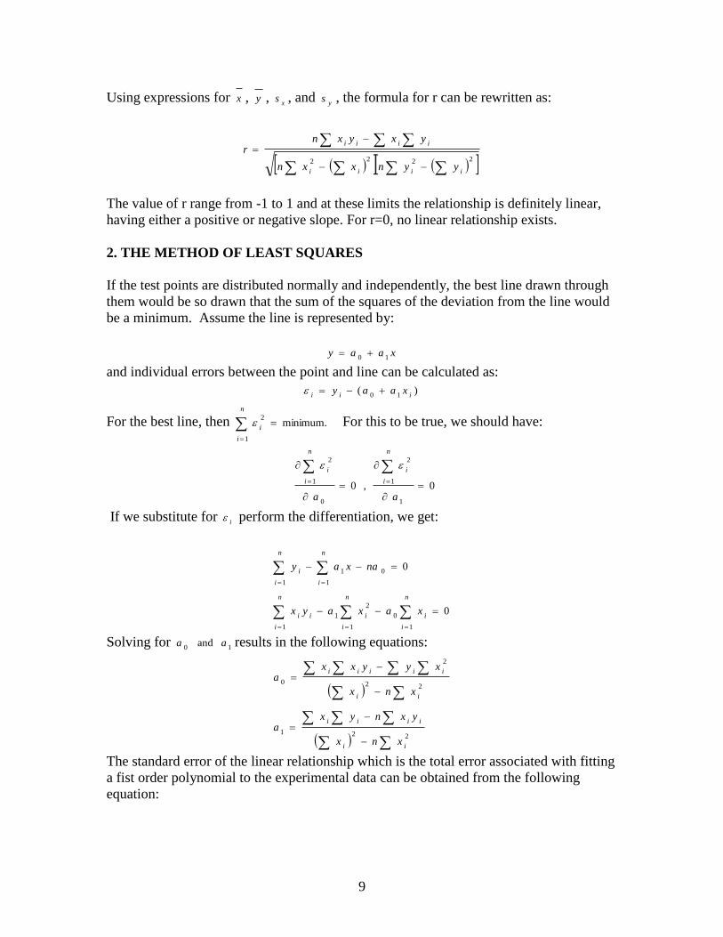
Using expressions for x , y , x

s , and y

s , the formula for r can be rewritten as:

2222

iiii

iiii

yynxxn

yxyxnr

The value of r range from -1 to 1 and at these limits the relationship is definitely linear,

having either a positive or negative slope. For r=0, no linear relationship exists.

2. THE METHOD OF LEAST SQUARES

If the test points are distributed normally and independently, the best line drawn through

them would be so drawn that the sum of the squares of the deviation from the line would

be a minimum. Assume the line is represented by:

xaay10

and individual errors between the point and line can be calculated as:

)(10 iii

xaay

For the best line, then minimum.

1

2

n

i

i For this to be true, we should have:

0

, 0

1

1

2

0

1

2

aa

n

i

i

n

i

i

If we substitute for i

perform the differentiation, we get:

0

0

1

0

1

2

1

1

0

1

1

1

n

i

i

n

i

i

n

i

ii

n

i

n

i

i

xaxayx

naxay

Solving for 1 0

and aa results in the following equations:

221

22

2

0

ii

iiii

ii

iiiii

xnx

yxnyxa

xnx

xyyxxa

The standard error of the linear relationship which is the total error associated with fitting

a fist order polynomial to the experimental data can be obtained from the following

equation:

10

Standard error = 2

1

2

01

2

n

axayii

The straight line relationships for various functions that are not linear can be obtained

with proper scales. Table 1 provides examples of values used to obtain the linear relations

for these non-linear functions.

________________________________________________________________________

Example: The following data fit an equation in the form of xaay 10

. Find the

equation and its correlation coefficients.

X Y

1.0 1.2

1.6 2.0

3.4 2.4

4.0 3.5

5.2 3.5

Solution: The coefficients of the equations are calculated from the following formulas:

22

2

0

ii

iiiii

xnx

xyyxxa and

2

21

ii

iiii

xnx

yxnyx

a

xi yi xiyi xi² yi²

1.0 1.2 1.20 1.00 1.44

1.6 2.0 3.20 2.56 4.00

3.4 2.4 8.16 11.56 5.76

4.0 3.5 14.00 16.00 12.25

5.2 3.5 18.20 27.04 12.25

summation, 15.2 12.6 44.76 58.16 35.70

With the substitution of the calculated data, the coefficients of the equations are

88.016.58*5)2.15(

)16.58(*)6.12()76.44(*)2.15(

20

a and 54.0

16.58*5)2.15(

)76.44(*5)6.12(*)2.15(

21

a

Thus, the equation of the line is xy 54.088.0 . The correlation coefficient between

the data set X and Y can be calculated as:

2222)()((

iiii

iiii

yynxxn

yxyxnr =0.94

_______________________________________________________________________

11

Function Abscissa Ordinate

xaay10

x y

a

kxy xlog ylog

ax

key x ylog

x

bay

x

1 y

bxa

xy

x

y

x

2cxbxay x

1

1

xx

yy

2cxbxa

xy

x

1

1

yy

xx

2

cxbxkey

x

1loglog yy

Table 1.

________________________________________________________________________

Example:

The following data fits the equation of the form bxaey . Find a and b.

Solution:

Taking the natural logarithm for both sides of the equation yields:

bxaebxaeaaeybxbx

lnln*lnlnln)ln(ln

This equation is similar to the equation of the line xaay 10

with y=lny, aa ln0

and ba 1

. Follow the same procedure as in the previous example, it gives

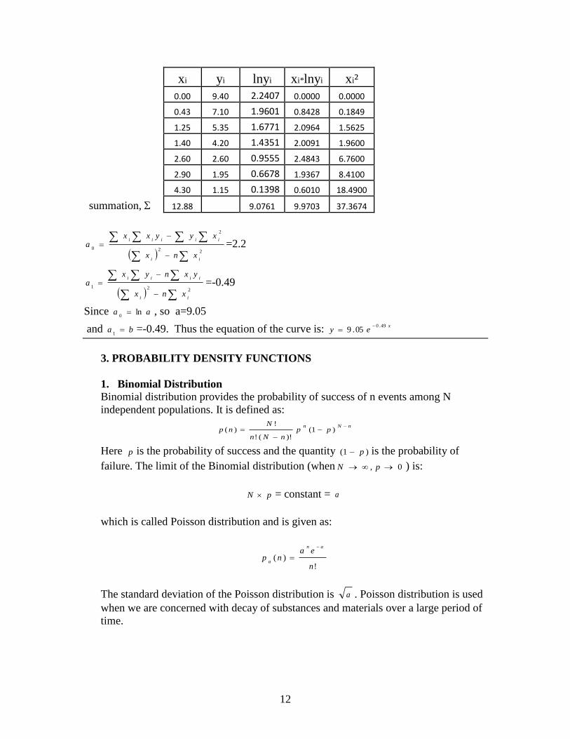
12

xi yi lnyi xi*lnyi xi²

0.00 9.40 2.2407 0.0000 0.0000

0.43 7.10 1.9601 0.8428 0.1849

1.25 5.35 1.6771 2.0964 1.5625

1.40 4.20 1.4351 2.0091 1.9600

2.60 2.60 0.9555 2.4843 6.7600

2.90 1.95 0.6678 1.9367 8.4100

4.30 1.15 0.1398 0.6010 18.4900

summation, 12.88 9.0761 9.9703 37.3674

22

2

0

ii

iiiii

xnx

xyyxxa =2.2

221

ii

iiii

xnx

yxnyxa =-0.49

Since aa ln0 , so a=9.05

and ba 1

=-0.49. Thus the equation of the curve is: xey

49.005.9

3. PROBABILITY DENSITY FUNCTIONS

1. Binomial Distribution

Binomial distribution provides the probability of success of n events among N

independent populations. It is defined as:

nNnpp

nNn

Nnp

)1(

)!(!

!)(

Here p is the probability of success and the quantity )1( p is the probability of

failure. The limit of the Binomial distribution (when 0, pN ) is:

pN = constant = a

which is called Poisson distribution and is given as:

!)(

n

eanp

an

a

The standard deviation of the Poisson distribution is a . Poisson distribution is used

when we are concerned with decay of substances and materials over a large period of

time.

13

2. Normal or Gaussian distribution

The mathematical representation of a normal or Gaussian distribution is:

2

2)(

2

1exp

2

1)(

xxp

xx

Most often, the “standard” normal distribution is used instead. To obtain the standard

normal distribution, let:

x

xz

With this transformation, the equation for the standard normal distribution becomes:

)2

exp(

2

1)(

2z

zp

For the standard normal distribution, the mean is zero, the standard deviation is one

and

0.1)( dzzp

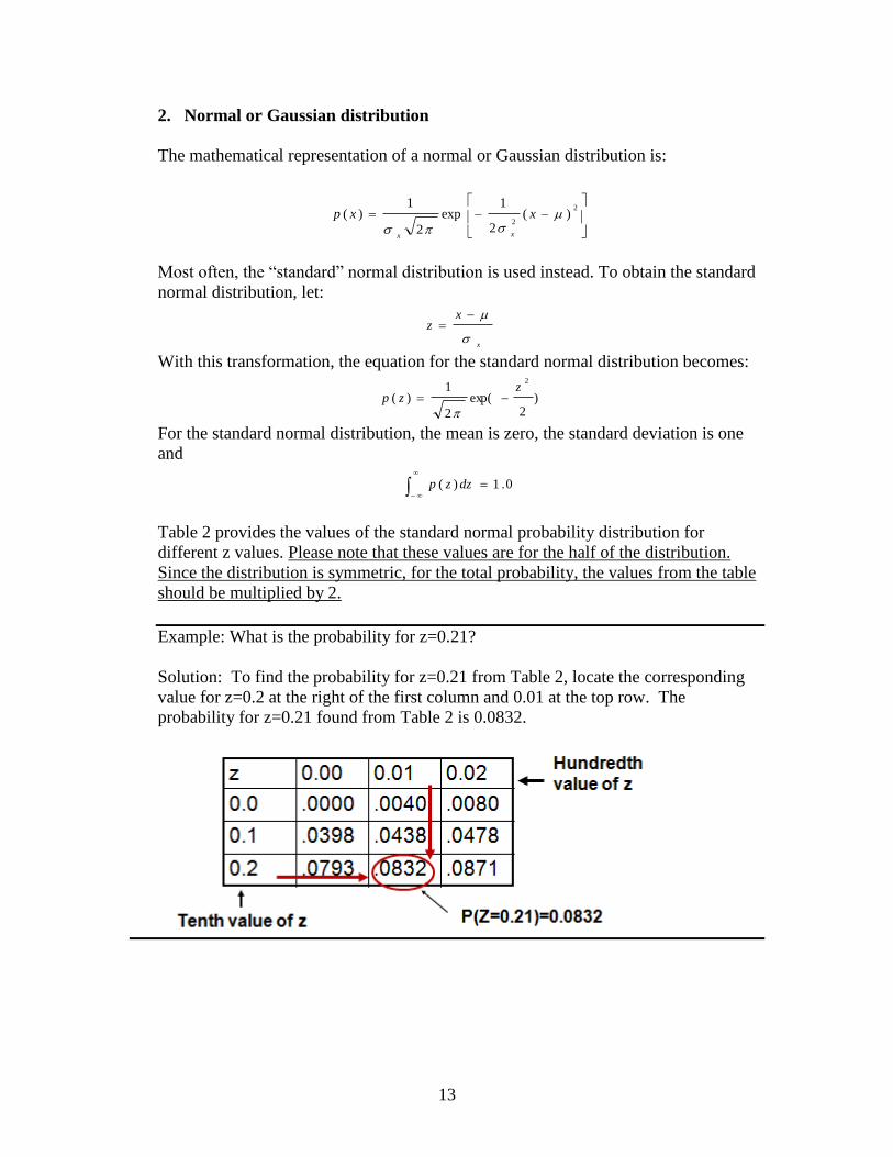
Table 2 provides the values of the standard normal probability distribution for

different z values. Please note that these values are for the half of the distribution.

Since the distribution is symmetric, for the total probability, the values from the table

should be multiplied by 2.

Example: What is the probability for z=0.21?

Solution: To find the probability for z=0.21 from Table 2, locate the corresponding

value for z=0.2 at the right of the first column and 0.01 at the top row. The

probability for z=0.21 found from Table 2 is 0.0832.

14

Table 2. Standard Normal Distribution

Example: What is the probability that an observation being more than two standard

deviations from the mean (p(x > µ + 2σ),p(x< µ-2σ))?

Solution: Substitute µ + 2σ and µ - 2σ for x in the equation

xz , then z

becomes >2 and <-2. From Table 2 for z=2, p(z) is 0.4772. Since the distribution is

symmetric, the probability of z> 2 is 0.5-0.4772=0.023 which is also equal to the

probability of z<-2. Thus, the total probability is 0.046 or approximately 0.05. 0.05

is equal to 5% or 1 in 20 which means in 20 observations; one can fall outside the two

standard deviation range.

15

Example: Calculate and plot the standard normal distribution for the following set of

data:

57.8, 24.8, 27.4, 36.5, 43.1, 44.0, 31.7, 40.1, 36.0, 47.2, 27.2

Solution: From the data, N=11, 8.371

1

n

i

ix

nx and

2

1

)(1

1xx

ns

n

i

ix

=9.96.

Using the equations s

xxz

and 2

2

2

1)(

z

ezP

, the values of z and P(z) for each

data are shown in the table below:

x z P(z) 57.8 2.0080 0.0531

24.8 -1.3052 0.1703

27.4 -1.0442 0.2313

36.5 -0.1305 0.3957

43.1 0.5321 0.3464

44.0 0.6225 0.3288

31.7 -0.6124 0.3308

40.1 0.2309 0.3885

36.0 -0.1807 0.3926

47.2 0.9438 0.2556

27.2 -1.0643 0.2265

0

0.05

0.1

0.15

0.2

0.25

0.3

0.35

0.4

0.45

-1.5 -1 -0.5 0 0.5 1 1.5 2 2.5

Z

P(Z

)

P(Z)

16

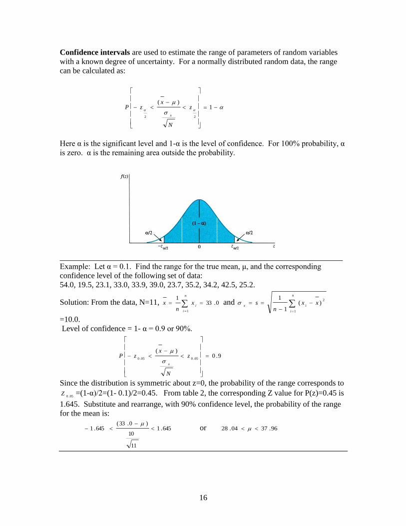
Confidence intervals are used to estimate the range of parameters of random variables

with a known degree of uncertainty. For a normally distributed random data, the range

can be calculated as:

1)(

22

z

N

xzP

x

Here α is the significant level and 1-α is the level of confidence. For 100% probability, α

is zero. α is the remaining area outside the probability.

_______________________________________________________________________

Example: Let α = 0.1. Find the range for the true mean, μ, and the corresponding

confidence level of the following set of data:

54.0, 19.5, 23.1, 33.0, 33.9, 39.0, 23.7, 35.2, 34.2, 42.5, 25.2.

Solution: From the data, N=11, 0.331

1

n

i

ix

nx and

2

1

)(1

1xx

ns

n

i

ix

=10.0.

Level of confidence = 1- α = 0.9 or 90%.

9.0)(

05.005.0

z

N

xzP

x

Since the distribution is symmetric about z=0, the probability of the range corresponds to

05.0Z =(1-α)/2=(1- 0.1)/2=0.45. From table 2, the corresponding Z value for P(z)=0.45 is

1.645. Substitute and rearrange, with 90% confidence level, the probability of the range

for the mean is:

645.1

11

10

)0.33(645.1

or 96.3704.28

17

3. Histogram: Histogram provides the probability of events within each increment. Histogram can

be used to check if the data follows a standard distribution or not. The following steps

can be used to draw a histogram:

(a) Choose a number of class intervals (usually between 5 and 20) that covers

the data range. Select the class marks which are the mid-point of the class

intervals. If you arrange data in ascending order, the first data should fall

in the first class interval.

(b) For each class interval, determine the number of data that fall within that

interval. If a data falls exactly at the division point, then it is placed in the

lower interval.

(c) Construct rectangles with centers at the class marks and areas proportional

to class frequencies. If the widths of the rectangles are the same, then the

height of the rectangles represent the class frequencies.

_______________________________________________________________________

Example: Develop the histogram for the following data:

3.0, 6.0, 7.5, 15.0, 12.0, 6.5, 8.0, 4.0, 5.5, 6.5, 5.5, 12.0

1.0, 3.5, 3.0, 7.5, 5.0, 10.0, 8.0, 3.5, 9.0, 2.0, 6.5, 1.0, 5.0

Solution:

Use the following guide to obtain the number of classes. It is recommended to use more

or fewer classes than the guide suggests if it makes the graph more descriptive.

Sample size Number of classes

10-20 5

20-50 6

50-100 7

100-200 8

200-400 9

400-700 10

In this example, the number of data is 25 so the number of classes is 6. The class interval

∆x =(Xmax-Xmin)/ number of class = (15.0-1.0)/6=2.333. For convenience, the class

interval is rounding up to 2.4 Beginning the first interval at the lowest value: Xmin-(the

smallest significant of data/2), that is

95.005.000.12

1.0

min1 xx

Next calculate the subsequent class interval points by adding ∆x.

35.34.295.012

xxx

75.54.235.323

xxx

15.84.275.534

xxx

55.104.215.845

xxx

95.124.255.1056

xxx

35.154.295.1267

xxx

The next step is to form the class subintervals. This is done using the method of left

incursion. For example, the first subinterval is from 0.95 up to but not including 3.35.

The second subinterval is from 3.35 up to but not including 5.75. And so on. For each

18

class subinterval, the class frequency is the number of data (or tally) occurs in the

subinterval and the class mark is a half of the class interval.

The histogram is constructed to show the data distribution over the interval 0.95 to 15.35.

The vertical axis is the class frequency and the horizontal axis is the data.

Students may try different number of class sizes to see if the graph is more descriptive. In

some cases, the relative class frequencies are preferred over the class frequencies.

Relative class frequencies make it easier to understand the distribution of the data and to

compare different sets of data. Relative frequencies are found by dividing each class

frequency by the sum of the frequencies.

Example: Plot a histogram for the above example using MS Excel.

The steps to plot the histogram using the MS Excel are as follows:

1. Highlight the columns of class marks and class frequency to plot XY (scatter)

chart.

0

1

2

3

4

5

6

7

8

9

0 1 2 3 4 5 6 7 8 9 10 11 12 13 14 15 16 17

Observed Data

Fre

qu

en

cy

19

2. Click the X axis to change the scale of minimum, maximum, and major unit

(unchecked Auto scaling)

First point X1

Last point Xn

Class width

20

3. Draw a rectangular box between the two endpoints of each class subinterval with the height matching the dot of each class mark.

_____________________________________________________________________

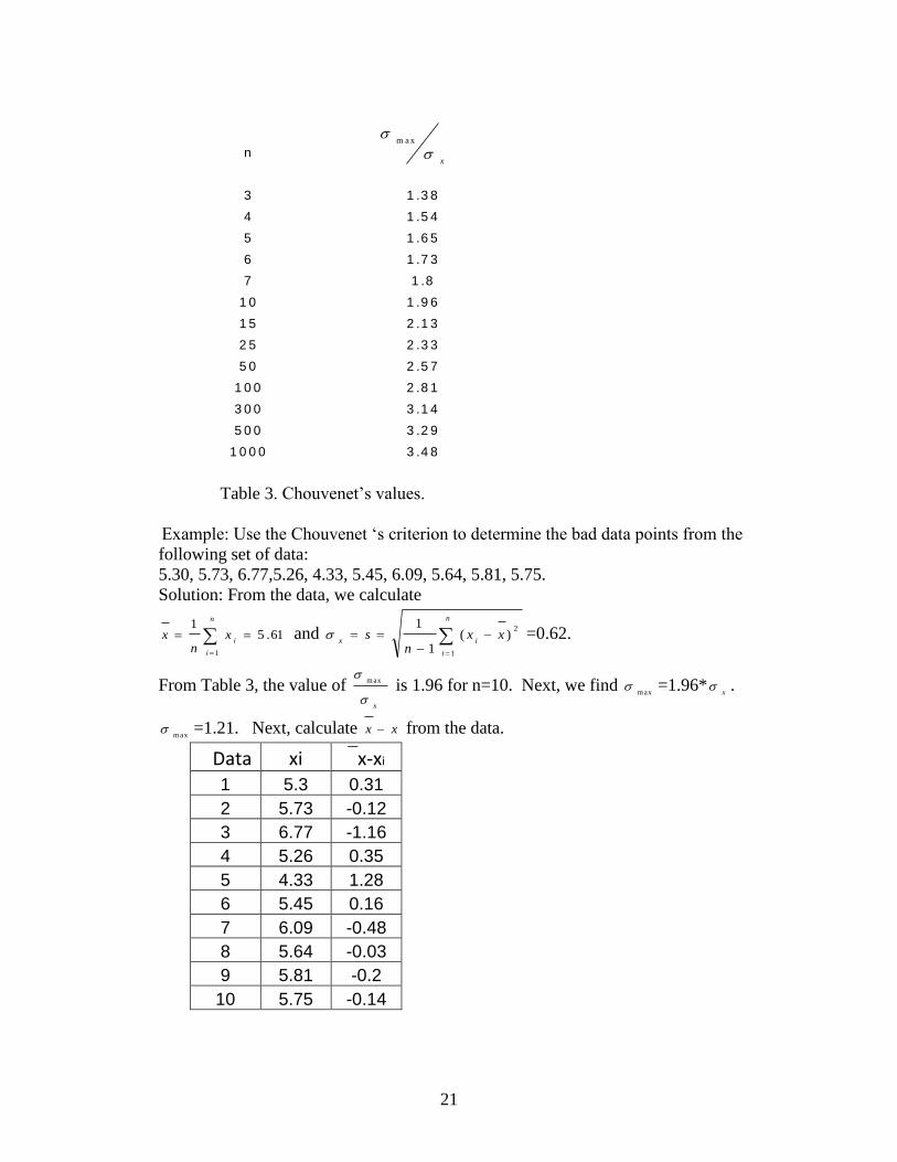
4. Chouvenet’s Criterion.

Assuming the data follows a normal distribution, Chouvenet’s Criterion is used to

eliminate bad data points. For any set of data, first the mean and standard deviation

of the entire population are calculated. Then the deviations of the individual data

points are compared with the standard deviation of the whole population according to

the following table, to accept or reject the data points. Here in the table, the ratio of

maximum allowable deviations to the standard deviation, x

max are given

according to the number of data points, n. Once the bad data points are eliminated,

then mean and standard deviation of the population are recalculated.

The following procedure can be used to assess a data point:

(a) For a sample population, calculate x

x and .

(b) Using sample population n, find x

max .

(c) Knowing x

, find max

.

(d) Calculate xx . Here x is the sample that you are assessing. If the difference is

larger than max

, the sample is discarded, otherwise it is retained.

0

1

2

3

4

5

6

7

8

9

0.95 3.35 5.75 8.15 10.55 12.95 15.35

data

Fre

qu

en

cy

21

Table 3. Chouvenet’s values.

Example: Use the Chouvenet ‘s criterion to determine the bad data points from the

following set of data:

5.30, 5.73, 6.77,5.26, 4.33, 5.45, 6.09, 5.64, 5.81, 5.75.

Solution: From the data, we calculate

61.51

1

n

i

ix

nx and

2

1

)(1

1xx

ns

n

i

ix

=0.62.

From Table 3, the value of x

max is 1.96 for n=10. Next, we find

max =1.96*

x .

max =1.21. Next, calculate xx from the data.

Data xi x-xi 1 5.3 0.31

2 5.73 -0.12

3 6.77 -1.16

4 5.26 0.35

5 4.33 1.28

6 5.45 0.16

7 6.09 -0.48

8 5.64 -0.03

9 5.81 -0.2

10 5.75 -0.14

n

3 1 .3 8

4 1 .5 4

5 1 .6 5

6 1 .7 3

7 1 .8

1 0 1 .9 6

1 5 2 .1 3

2 5 2 .3 3

5 0 2 .5 7

1 0 0 2 .8 1

3 0 0 3 .1 4

5 0 0 3 .2 9

1 0 0 0 3 .4 8

x

m a x

22

Since the data number 5 has xx =1.28, larger than the value of max

= 1.21,

Therefore, the data 4.33 is considered as bad data point.

5. Chi-square (2

) distribution.

It is used as a test of “goodness of fit”, to assess whether data matches a specific

distribution. It is defined as:

n

i 1 i

2

i2

(expected)

expected)-observed(

Here, the expected values are from the specific distribution. The Chi-square statistics

is:

F

z2

2

Here z is taken from standard normal distribution and F is degrees of freedom. The

Chi-square distribution is always positive. The smaller the 2 value the better the fit

between the experimental data and the expected distribution. If 2 is zero, then we

have a perfect match between our experimental data and the specific distribution. For

large number of samples, the Chi-square distribution assumes the bell shape of the

normal distribution. The 2 table (table 4) on the following page provides the

probability p that this value of 2 or higher values could occur. To use this table, first

the degrees of freedom and the 2 are calculated, then the probability p is obtained

from the table which is the probability of the goodness of fit.

23

DF 0.995 0.99 0.975 0.95 0.90 0.10 0.05 0.025 0.01 0.005

1 --- --- 0.001 0.004 0.016 2.706 3.841 5.024 6.635 7.879

2 0.010 0.020 0.051 0.103 0.211 4.605 5.991 7.378 9.210 10.597

3 0.072 0.115 0.216 0.352 0.584 6.251 7.815 9.348 11.345 12.838

4 0.207 0.297 0.484 0.711 1.064 7.779 9.488 11.143 13.277 14.860

5 0.412 0.554 0.831 1.145 1.610 9.236 11.070 12.833 15.086 16.750

6 0.676 0.872 1.237 1.635 2.204 10.645 12.592 14.449 16.812 18.548

7 0.989 1.239 1.690 2.167 2.833 12.017 14.067 16.013 18.475 20.278

8 1.344 1.646 2.180 2.733 3.490 13.362 15.507 17.535 20.090 21.955

9 1.735 2.088 2.700 3.325 4.168 14.684 16.919 19.023 21.666 23.589

10 2.156 2.558 3.247 3.940 4.865 15.987 18.307 20.483 23.209 25.188

11 2.603 3.053 3.816 4.575 5.578 17.275 19.675 21.920 24.725 26.757

12 3.074 3.571 4.404 5.226 6.304 18.549 21.026 23.337 26.217 28.300

13 3.565 4.107 5.009 5.892 7.042 19.812 22.362 24.736 27.688 29.819

14 4.075 4.660 5.629 6.571 7.790 21.064 23.685 26.119 29.141 31.319

15 4.601 5.229 6.262 7.261 8.547 22.307 24.996 27.488 30.578 32.801

16 5.142 5.812 6.908 7.962 9.312 23.542 26.296 28.845 32.000 34.267

17 5.697 6.408 7.564 8.672 10.085 24.769 27.587 30.191 33.409 35.718

18 6.265 7.015 8.231 9.390 10.865 25.989 28.869 31.526 34.805 37.156

19 6.844 7.633 8.907 10.117 11.651 27.204 30.144 32.852 36.191 38.582

20 7.434 8.260 9.591 10.851 12.443 28.412 31.410 34.170 37.566 39.997

21 8.034 8.897 10.283 11.591 13.240 29.615 32.671 35.479 38.932 41.401

22 8.643 9.542 10.982 12.338 14.041 30.813 33.924 36.781 40.289 42.796

23 9.260 10.196 11.689 13.091 14.848 32.007 35.172 38.076 41.638 44.181

24 9.886 10.856 12.401 13.848 15.659 33.196 36.415 39.364 42.980 45.559

25 10.520 11.524 13.120 14.611 16.473 34.382 37.652 40.646 44.314 46.928

26 11.160 12.198 13.844 15.379 17.292 35.563 38.885 41.923 45.642 48.290

27 11.808 12.879 14.573 16.151 18.114 36.741 40.113 43.195 46.963 49.645

28 12.461 13.565 15.308 16.928 18.939 37.916 41.337 44.461 48.278 50.993

29 13.121 14.256 16.047 17.708 19.768 39.087 42.557 45.722 49.588 52.336

30 13.787 14.953 16.791 18.493 20.599 40.256 43.773 46.979 50.892 53.672

40 20.707 22.164 24.433 26.509 29.051 51.805 55.758 59.342 63.691 66.766

50 27.991 29.707 32.357 34.764 37.689 63.167 67.505 71.420 76.154 79.490

60 35.534 37.485 40.482 43.188 46.459 74.397 79.082 83.298 88.379 91.952

70 43.275 45.442 48.758 51.739 55.329 85.527 90.531 95.023 100.425 104.215

80 51.172 53.540 57.153 60.391 64.278 96.578 101.879 106.629 112.329 116.321

90 59.196 61.754 65.647 69.126 73.291 107.565 113.145 118.136 124.116 128.299

100 67.328 70.065 74.222 77.929 82.358 118.498 124.342 129.561 135.807 140.169

Table 4. Chi –square table.

24

Example: A random sample of furniture defects from a shipping company was recorded. The

observed and expected defects were classified into four types: A,B,C, and D.

Does the observed data differ significantly from the expected data with significant level α=0.05?

Solution:

In order to compare the goodness-of-fit test, the total counts of observed data must

agree with the total counts of expected data.

Then calculate the Chi-square:

90

)9081(

8

)812(

20

)2018(

82

)8289(

exp

)exp(22222

2

ected

ectedobserved

=3.698

The number of recording for each set of observed and expected data is 4. Thus, n=4.

Furthermore, we impose one restriction on the data: the number of recording is fixed. Thus k=1

and the degree of freedom is dF = n-k = 4-1=3. Assuming a significant level of 0.05, the critical

value for from Table 4 is 7.815. Since the calculated value 3.698 is less than the critical value

7.815. Therefore, the observed distribution is a good fit with the expected distribution.

6. Student t-distribution.

It is the ratio of the normal to chi-square distribution. It is used for small sample. It is flatter

than the normal distribution with more population towards the tails of the distribution. It is

written as:

s

xxt

i

F

As the sample size increases, the frequency around the mean increases, while the number of

data under its tails decreases, and it approaches the normal distribution curve. Table54

provides the values for the student t distribution.

25

Table 5. Student t distribution.

t-Test Comparison of Different samples

t-Test comparison is used to determine if significant difference exists between two samples.

The following steps describe the process for determining whether the two samples within a

confidence level are statistically the same or different:

1. Determine the number of sample, n, the mean x , and the standard deviation s for each

sample.

2. Calculate the t value from the following equation:

26

21

2

2

2

1

2

1

21

n

s

n

s

xxt

3. Determine the degrees of freedom, F, from the following equation:

112

2

2

2

2

1

2

1

2

1

2

2

2

2

1

2

1

n

n

s

n

n

s

n

s

n

s

F

4. Select a confidence level

5. Use the F value and the proper confidence level corresponding to half of the significant

level selected to find a new t value from the student t table (table 5).

6. If the t value from step 2 is less than the t value from step 5, then the two samples are

statistically the same. Otherwise they are different.

Note: The significance level is the probability remaining under the tail of the distribution. For

90% confidence, the significance level is 10%.

__________________________________________________________________________

Example:

The following two sets of data provide the statistics of the production lines:

Set 1: 80, 86, 80, 86, 85, 78, 75, 91, 89, 81

Set 2: 74, 81, 73, 78, 79, 76, 78, 84, 80, 74

With 95% confidence level, decide (show the calculations) whether the two samples are the

same or different.

Solution:

For the set 1, n1=10, 1.831

1

1

n

i

ix

nx and

2

1

1)(

1

1xx

ns

n

i

ix

=5.09.

For the set 2, n2=10, 7.771

1

2

n

i

ix

nx and

2

1

2)(

1

1xx

ns

n

i

ix

=3.50

Calculate the t and F values from equation above:

t=2.77

F=15.95

The degree of freedom is rounded down to 15. With 95% confidence level, α=0.05 and

α/2=0.025, the t value from the student t table (table 5) is t=2.131.

Since the t value from the formula is higher than the t value from the table, the two sets are

statistically different. ______________________________________________________________

27

Exercises

1. For the following data, find the mean, median, variance and standard deviation.

21, 20, 8, 14, 6, 19, 24.

2. Find mean, standard deviation, mode, median, and coefficient of variation of the

following data. Develop a histogram.

10.256, 10.855, 10.115, 9.995, 10.556, 10.188, 10.100, 10.656, 10.050, 9.995, 10.580,

10.655, 10.100, 10.650, 10.660, 10.755, 10.800, 10.456, 10.582, 10.338, 10.400, 10.455,

10.256, 10.588, 10.399

Note that the accuracy of the data is to 3rd

decimal place and thus your answer should have a

maximum accuracy of the same significance.

3. For 800 respondents to an inquiry of their age, results show a mean of 42 years and a

standard deviation of 5 years. How many respondents fall between 2 standard deviation

from the mean?

4. Specific heat of any substance is defined as the change in heat per unit mass per units rise

in temperature. The following data represents the change in specific heat of a substance

with temperature:

T (C) = 40, 50, 60, 70, 80, 90, 100

Specific Heat = 1.58, 1.60, 1.63, 1.67, 1.7, 1.72, 1.78

Plot temperature vs. specific heat. Find a first order polynomial and the standard error for

the data. What is the correlation coefficient?

5. Given the following data, find the straight-line equation using the least square method.

Find the standard error.

X= 1, 2, 3, 4, 5, 6, 7, 8, 9, 10.

Y=2.5, 4.8, 6.5, 7.9, 9.7, 11.1, 12.7, 14.7, 16, 17.4.

6. The following data fit an equation in the form of bxaey

. Find a and b.

X= 0, 0.5, 1.0, 1.5, 2.0

Y=1.3499, 1.7333, 2.2255, 2.8577, 3.6693

7. Calculate the correlation coefficient for the following data:

X=0, -1, -2, -3, -2, -2, 0, 1, 2, 3, 2, 1

Y=3, 2, 1, 0, -1, -2, -3, -2, -1, 0, 1, 2

28

8. Calculate the correlation coefficient for the following data:

X=1, 5, 10, 15

Y=7, 19, 34, 49

Can the data be represented with a linear equation? If so, find the equation.

9. Given the following table for grades on a test, draw histogram and calculate mean and

standard deviation.

X F

95-100 2

85-90 4

75-80 16

65-70 22

55-60 35

45-50 43

35-40 32

25-30 20

15-20 6

10. Two sets of samples for length are taken from a production line with the

following statistics

24n cm 0.02 3.611

17n cm 0.06 3.632

222

111

X

X

With 95% and 65% confidence levels, determine whether the two samples are

statistically the same or different.

11. Find the range for the population mean value with 95% and 65% confidence intervals for

each set of data.

24n cm 0.02 3.611

17n cm 0.06 3.632

222

111

X

X

12. A packaging company conducts a survey for the two new package designs for lunch

boxes in a supermarket. The results are as follows:

Design1 158.5 138.4 168.1 149.4 145.8 168.7 154.4 162.9

Design2 150.3 155.4 151.6 158.8 151.4 150.8 161.4 157.6 156.8 147.6

a. What is the range of the true (or population) mean of the data in each design for

13.

80% confidence level?

b. Calculate the standard normal distribution z and P(z) for each data set.

29

Chapter 2

2

MEASUREMENT UNCERTAINTY

30

2.1. MEASUREMENT UNCERTAINTY

The term uncertainty is used to describe variation in the measurement or control of any quantity

associated with an experiment. Thus, uncertainty is a measure of the accuracy of the

experimental data. Specifically, it is an estimate of the maximum error which might reasonably

be expected from a set of measurements. It is important to estimate the uncertainty associated

with a measurement and to determine ways to reduce it.

Similar to an experiment, numerical analysis of any problem also contains errors associated with

the assumption(s) made, the method of analysis, the type of grid and the number of iterations that

are used, etc. It is also very important that results from any numerical analysis also presented

with their uncertainty.

Measurement of any property contains errors. The errors are the differences between the

measured values and the true value. The true value is either given or estimated from previous

repeated experiments, or assumed to be the reasonable human error associated with the

limitations of the measuring instrument being used. For example, the uncertainty of an

instrument such as a digital pressure transducer will typically be given in the operating manual.

If it is not, then a set of experiments that compare the reading from the transducer to a known

input can be devised that allows estimation of the uncertainty of the transducer. In the case of a

simple measurement device, such as a ruler, the uncertainty can be estimated by determining

how closely an individual can reasonably read the graduations on the ruler.

Error in a measurement has two components: fixed or bias error and random or precision error

(repeatability). Bias error is the difference between the mean value, x , of the measurements and

the actual value of the quantity being measured. The mean value is estimated from the following

equation:

N

i

ix

Nx

1

1 (2-1)

In this equation, N is the number of samples and i

x is the value for each measurement. With

thirty or more samples, the mean is often used as an estimate of the true value of a measurement

Bias is the systematic error. In repeated measurements at the same conditions, bias error is the

same for all of them. The bias can not be determined unless we know the true value. Many

experimental apparatus can operate within a special range of experimental conditions. If the

environment changes, the accuracy of the equipment will affected, and thus the bias will change.

Bias errors can be eliminated by calibration if they are large and known. Small unknown biases

contribute to the bias limit.

Large unknown biases usually come from human errors in data processing, incorrect handling

and installation of instrumentation, and unexpected environmental disturbances such as changes

31

in humidity, temperature, or Barometric pressure. A well controlled environment should not have

large unknown biases.

The major sources of bias error are: 1) Nonlinearity, 2) poor calibration, 3) Hysteresis, and 4)

Drift.

The output of a device should be linearly proportional to its input. However, all devices deviate

from linearity. Nonlinearity can always be described as a combination of an offset from the ideal

linear response and a wobble about the ideal linear response. The departure from linearity may

be classified in one of two ways: Independent of reading and dependent on reading. When an

independent of reading classification is specified, it means that the maximum deviation from

linearity is less than a certain percentage of full scale. The a dependant on reading classification

is specified, it means that the maximum deviation from the measurement reading is less than a

certain percentage of that particular reading.

Calibration is used to determine the response of a device to a known input. Once this response is

known, the device can be used to determine the value of an unknown input. The accuracy of the

relationship of the response determined during calibration directly affects the accuracy of the

measurement.

The response of a measurement device has hysteresis when the output of the device is dependent

on the direction from which the corresponding input is approached. Specifically, a reading near

the midrange of an instrument will have two different values depending on whether the reading

is achieved from descending from full scale or achieved from ascending from zero. The usual

cause of hysteresis is friction or inertia.

Drift is used to describe an error that manifests itself as a change in output for a fixed input over

time. Drift can be observed by maintaining a steady input while monitoring the output.

Generally, drift is due to the effect of temperature change during the warm up of the electronic

components in a device.

Precision error is the variation between repeated measurements. The estimated standard

deviation from the mean, S, is used as a measure of the precision error. A large standard

deviation means a large scatter in the measurements. The standard deviation is defined as:

2

1

1

2

1

N

i

i

N

xxS (2-2)

Here, xi, x and N are respectively the individual, the estimated average, and the number of data

points. Figure 2-1 shows precision and bias errors of a set of measurements.

If the number of data points is large and they follow a normal distribution curve, and if there is

no bias, the mean is the estimated average of the data points and 2 S is the uncertainty interval

with 95% confidence level or 20:1 odd. The 20:1 odd means that if the experiment is repeated 20

times, there is a possibility that 19 times the data falls within the range x S 2 and there is only

once that it will be out of this range.

32

Experiments are either single sample or multiple samples. In single sample experiments, test

point is run once. In multiple sample experiments, each test point is run more than once.

Research in fluid mechanics and heat transfer are usually single sample experiments.

In single sample experiments, the precision error is dominant. In contrast, in multiple samples

experiments, the fixed error is dominant since in multiple measurements of a point, the random

errors are averaged out.

Figure 2-1

2.2. UNCERTAINTY IN EXPERIMENTAL RESULTS

In general, the results of experiments are calculated from a set of measurements:

),,,(21 N

xxxRR (2-3)

The uncertainty in experimental results should have the same odd or confidence level as the

measurements. The uncertainty in the result is expressed as:

2

1

1

2

N

i

i

i

xx

RR

(2-4)

This method is called Root Sum Square (RSS). The partial derivative of the result, R, with

respect to the measurement xi,

R

xi

, is called the sensitivity coefficient. xiis the uncertainty in

the variable xi. The sensitivity coefficient weights the value of the uncertainty of the variable

corresponding to the dominance of the variable in the fundamental equation.

The RSS method can be used to estimate uncertainty in experimental results if: (a) measurements

are independent and repeated measurements of each quantity follow a normal distribution and (b)

the same odds are used for estimating the uncertainty of each measurement. The RSS equation is

generally used in the normalized form as:

33

2

1

22

22

2

2

11

1

N

u

Nx

R

R

Nx

ux

R

R

xu

x

R

R

x

Ru

(2-5)

Here, uR

and uiare, respectively, the uncertainties in the result and in the measurement of x

i.

Example: The following equation is used in an orifice plate to calculate the volume flow rate of

the fluid:

PCAQ

Here is pressure differential, ρ is density and Q is the volume flow rate. If ΔP = 250±5 Pa

and ρ=1.195± 0.01 kg/m³, find the volume flow rate and its variations. C and A are constants at

0.7 and 0.01m² respectively.

Solution:

The volume flow rate is calculated using the average or nominal values of the given data.

smmkg

mNm

PCAQ

3

3

2

2101.0

195.1

250*)01.0(*)7.0(

In this problem, the uncertainty for volume flow rate is a function of the pressure and density

where these two variables have its measurement uncertainty. The uncertainty equation for Q is:

2

1

22

U

Q

QU

P

Q

Q

PU

PQ

Taking the partial derivative and then substitution yields

1

2

2

1

PCA

P

Q →

2

1

22

CA

PCA

P

P

Q

Q

P

2

2

1

2

PPCAQ

→ 2

1

222

PCA

PCA

Q

Q

02.0250

5

PU (2%)

0084.0195.1

01.0

U (8.4%)

Thus, the uncertainty equation for Q becomes:

34

01084.02

1

2

12

1

22

UUU

PQ or 1.08%

If both bias and precision errors are considered, first the root sum square of the biases and the

precision are calculated separately as:

2

1

1

2

2

1

1

2

N

i

x

i

i

R

N

i

x

i

i

R

i

i

x

R

R

x

x

R

R

xS

(2-6)

Then, depending on the confidence level, one of the following equations is used to estimate the

total uncertainty, uR

.

u tSR R R ( ) for 95% confidence level (2-7)

Here, SR and

R are respectively the precision and bias errors in the final result, and t is from

the student t distribution. The student t distribution is used because the distribution of the

precision error does not have a normal distribution. It has a distribution that is dependent on the

number of samples and, therefore, the degrees of freedom. Thus, t in Equation 2-7 is dependent

on the number of samples collected. The shape of the student t distribution is very similar to the

normal distribution, but has a greater width to its bell shape.

For samples higher than 30, t is assumed to be 2. For samples less than 30, t is obtained from the

student t distribution table, using the required confidence level and the number of degrees of

freedom., . For single sample experiments, the sample number is the number of degrees of

freedom. Table 2-1 presents the values for t in terms of the degrees of freedom for the 95%

confidence level.

35

Figure for Table 2-1

Table 2-1

Equation 2-7 can be used to estimate the overall uncertainty, provided that the bias limit is

symmetrical about the measurement. If the bias limit is nonsymmetrical, then the upper and

lower limits of the uncertainty interval should be specified separately. Figure 2-2 shows the

measurement uncertainty for symmetrical and nonsymmetrical biases.

36

Figure 2-2

If the number of independent sets of measurements for calculating a quantity is more than one,

then first the cumulative degrees of freedom for the measurements is calculated from the Welch-

Satterthwaite equation as:

37

N

i i

i

i

R

v

S

Sv

1

4

22)(

(2-8)

Then, from the student t distribution the t values are found for the 95% confidence level. The

overall bias and precision errors are found from the following equations:

2

i

i

N

SS

(2-9)

Here, ii

S , , and N are respectively the overall precision and bias errors and the number of

independent sets of measurements. Assuming symmetrical bias, the uncertainty interval is:

)( tSu (2-10)

38

REFERENCES

1. Abernethy, et al, 1973, “Handbook, Uncertainty in Gas Turbine Measurements,” Arnold

Engineering Development Center Report No. AEDC- TR-73-5.

2. Abernethy, R.B., Benedict, R.P., and Dowdell, R.B., 1985, “ASME Measurement

Uncertainty,” ASME Journal of Fluids Engineering, Vol. 107, pp. 161-164.

3. Kline, S.J., 1985, “The Purpose of Uncertainty Analysis,” ASME Journal of

Fluids Engineering, Vol. 107, pp. 153- 160.

4. Kline, S.J., and McClintock, F.A., 1953, “Describing Uncertainties in Single

Sample Experiments,” Mechanical Engineering, pp. 3-8.

5. Moffat, R.J., 1988, “Describing the Uncertainties in Experimental Results,”

Experimental Thermal and Fluids Science, Vol. 1, pp. 3-17.

39

EXAMPLES

1. The Bernoulli’s equation given below has been used extensively to obtain the mean

velocity from dynamic pressure measurement. What is the uncertainty in the U, given that the

uncertainties in U, P , and are respectively u , p and .

2

1

2

PU

Solution:

But,

Then,

2

1

22

2

1

2

1

Pu

U

2. What is the uncertainty in the Reynolds number given as:

UD

DRe

The uncertainties in ,,, DU and are respectively ,,, DU and .

21

22

U

Up

P

U

U

Pu

U

2

1

2

2

12

2

1

2

1

2

1

U

P

PU

P

P

U

U

P

2

1

2

2

112

2

1

2

1

2

1

U

P

P

U

U

U

40

Solution:

21

2222

Re

Re

Re

Re

Re

Re

Re

Re

Re

D

D

D

D

D

D

D

D

DD

DU

U

Uu

D

But,

1Re

1Re

Re

D

D

D

UD

U

U

1Re

1Re

Re

D

D

D

UD

D

D

1Re

1Re

Re

D

D

D

UD

then,

3. What is the uncertainty of the increase in length L, with a wire with diameter D, and a

load of F?

Uncertainty in diameter is d, the length is L, and the uncertainty in F is F. Assume

that the E modulus of elasticity has no uncertainty (E=0).

eLLeL

L

1Re

1Re

Re

D

D

D

UD

21

2222

Re DUu

D

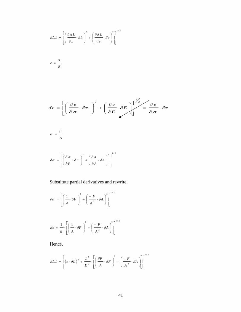
41

2/122

e

e

LL

L

LL

E

e

A

F

2/122

A

AF

F

Substitute partial derivatives and rewrite,

2/12

2

2

1

A

A

FF

A

2/12

2

2

11

A

A

FF

AEe

Hence,

2/1

2

2

2

2

2

A

A

FF

A

F

E

LLeL

eE

E

eee

21

2

42

4. A hook carries a load of F pounds. What is the uncertainty of the calculated maximum

stress in the vertical portion of the hook? The hook has an a x a square cross-section and the

radius in the bend of the hook is R. The uncertainty in length measurement is a, in radius is R

and the uncertainty in force measurement is F.

Substituting into the uncertainty equation, :

I

yM

A

F

2/1

22222

I

IM

My

yF

FA

A

A = a2

aaa

AA

2

2/12

2

ay

aaa

yy

2

1

2/12

RFM

2/1

22

2/122

)( RFFRRR

MF

F

MM

1212

43ahb

I

43

aa

Ia

II

12

43

2/12

2/12

3

2

2

2/122

222

212

4

222

112

a

a

I

aMRFFR

I

aa

I

MF

Aa

A

aF

Rearrange,

2

12

2

4

22

2222

26

1

22

112

a

I

aMRFFR

I

aa

I

MF

Aa

A

aF

44

Chapter 3

3

ELECTRICAL TRANSDUCERS

45

3.0. ELECTRICAL TRANSDUCERS

There are two general types of electrical transducers; active and passive transducers. Active

transducers generate an electromotive force (emf) when the physical property of interest is being

sensed. The sensitivity of the active transducers is expressed as the change in electrical output to

the change in physical input. Examples of the active transducers are thermocouples and

piezoelectric transducers.

Passive transducers produce a change in resistance, inductance, or capacitance by the physical

effect of the property being measured. The change is then being sensed by a voltage device. The

relative sensitivity of the passive transducers is expressed as Z

Z to the change in physical input.

Here Z is the internal impedance of the system. Examples of passive transducers are resistance,

inductive and capacitive transducers.

3.1. Active Transducers

3.1.1. Thermocouple

When two dissimilar metals are in contact with each other, they form a thermocouple. When

thermocouple is exposed to a temperature variation, an emf is generated. The net voltage

generated is:

dTeeE

LT

T

net)(

0

21

Here L

TTee and ,,021

are voltages generated along each wire and the reference temperatures.

The above equation can be used if only two wires are used and the materials are

homogeneous and voltage output is not a function of position along the wire. Each wire

begins at temperature 0

T and ends at temperature L

T .

For construction “positive” and a “negative” metal should be used. A “positive” metal is the

one that the emf increases with temperature along its length. On the other hand a “negative”

metal is the one that the emf decreases with the temperature along its length. Figure 1 shows

characteristics of alloys most commonly used for thermocouple constructions.

Figure 3.1. Characteristics of metal alloys with temperature.

46

Figure 2 shows a thermocouple that measures hot

T relative to ambient temperature amb

T as

the reference temperature.

Figure 3.2.

However, if other reference temperatures (i.e. ice bath) are required, then the configurations

shown in Figure 3 can be used. Here the copper extension wires do not affect the emf output.

Most electronic devices that are used for temperature measurements in conjunction with

thermocouples have already been calibrated to display temperature with reference to the ice-

bath condition.

Figure 3.3.

Depending on the temperature range and sensitivity different materials are used for the wires.

Table 1 shows different thermocouples with their corresponding range and sensitivity.

Factors that can introduce errors in temperature measurements are:

(a) Wire inhomogeneties from defect, plastic deformation, and a change in chemical

composition;

(b) Straining of the wires due to variations in cold working of the wires or from vibration;

(c) The exposure of the thermocouple to electrolytes, which results in significant addition in

the emf output.

47

Type Materials Range Sensitivity

C

C

Nickel-10%Chromium(+)

E Vs -100 to 1,000 5.0

Constantan(-)

Iron(+)

J Vs 0 to 760 1.0

Constantan(-)

Nickel-10%Chromium(+)

K Vs 0 to 1,370 7.0

Nickel-5% (-)

Platinum-13% Rhodium (+)

R Vs 0 to 1,000 5.0

Constantan(-)

Platinum-10% Rhodium (+)

S Vs 0 to 1,750 0.1

Constantan(-)

Copper(+)

T Vs -160 to 400 5.0

Constantan(-)

Table 3.1. Different thermocouples.

48

3.1.2. Law of Thermoelectricity

1. The thermal emf of a thermocouple with junctions at 4,1

T and 3

T is not affected by

temperature elsewhere in the circuit (i.e. 2

T ), provided that the two metals used are

homogeneous.

Figure 3.4.

2. If a third homogeneous wire C is inserted into either metal A or B, as long as the two new

junctions (2) and (4) are at the same temperatures, the net emf of the circuit is unchanged,

even if C is at different temperature than the measuring and reference temperatures.

Figure 3.5.

3. If wire C is inserted between A and B at one of the junctions, as long as the new junctions

(2) and (4) are at the same temperature, the net emf of the circuit will be the same as

before.

Figure 3.6.

3.1.3. Piezoelectric Transducers

The piezoelectric effect is the ability of a material to generate an electric potential when

subjected to a mechanical straining or to change dimension when subject to a voltage

potential. The sensing elements have high sensitivity and resonant frequency and respond

both to static and dynamic loadings. Examples of piezoelectric materials are quartz, ceramic,

49

sugar, and ammonium dihydrogen phosphate. Figure 7 shows various deformations of a

piezoelectric plate. The material that is widely used is quartz due to its stability. However,

quartz generates a very low voltage output. Generally a miniature voltage amplifier is packed

with the device to increase its sensitivity. Quartz is usually shaped into a silvered face thin

disk with electrodes attached to each face. The disk thickness depends on the required

frequency response since different thick nesses resonate at different frequencies.

Piezoelectric devices are used for force, pressure, stress, acceleration, and sound and noise

measurements, among others. Piezoelectric pressure transducers with quartz crystal can

measure pressure up to 100,000 psi while the ones with the ceramic can measure up to a

maximum pressure of 5,000 psi.

The piezoelectric effect is not present, until the element is subjected to a polarizing treatment.

The usual procedure is to heat the element to a temperature above 120 C and then apply a

high voltage (in the order of 10,000 Volts/cm thickness) to the element and then cool it down

to room temperature.

Figure 3.7. Configurations used for different measurements.

All piezocrystals have a Curie-point temperature, above which the structure of the crystal

changes and the piezoelectric effect is lost. Thus, care should be made not to expose the

crystal to a temperature above the Curie-point temperature.

The performance of these transducers can be improved by stacking multi-crystals together

under the same load.

3.2.0 Passive Transducers

3.2.1. Variable Resistance Transducers

The equation governing the operation of variable resistance transducers is:

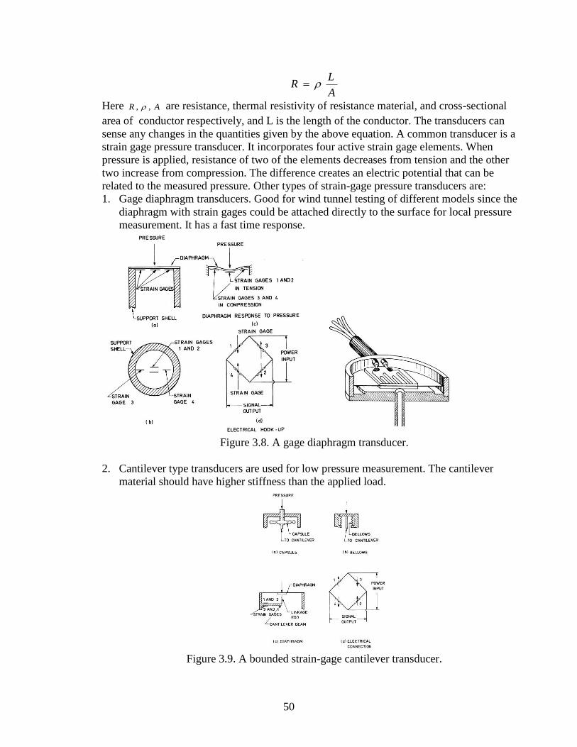
50

A

LR

Here AR , , are resistance, thermal resistivity of resistance material, and cross-sectional

area of conductor respectively, and L is the length of the conductor. The transducers can

sense any changes in the quantities given by the above equation. A common transducer is a

strain gage pressure transducer. It incorporates four active strain gage elements. When

pressure is applied, resistance of two of the elements decreases from tension and the other

two increase from compression. The difference creates an electric potential that can be

related to the measured pressure. Other types of strain-gage pressure transducers are:

1. Gage diaphragm transducers. Good for wind tunnel testing of different models since the

diaphragm with strain gages could be attached directly to the surface for local pressure

measurement. It has a fast time response.

Figure 3.8. A gage diaphragm transducer.

2. Cantilever type transducers are used for low pressure measurement. The cantilever

material should have higher stiffness than the applied load.

Figure 3.9. A bounded strain-gage cantilever transducer.

51

3. Pressure vessel transducers. Good for high pressure measurements. The pressure range is

1,000 to 100,000 psi. It consists of a cylindrical element with one end closed and the

pressure is applied to the open end. It has two active strain gages and two dummy ones

(to complete the bridge), attached to the outside surface.

Figure 3.10. A pressure vessel transducer.

4. Embedded strain-gage transducers. It consists of a shell with epoxy resin as embedding

material. The strain gages are placed inside the embedding material. When pressure is

applied, the strain gage resistances change which can be calibrated to measure applied

pressure. It has a fast response and has a maximum pressure not exceeding 750 psi.

Figure 3.11. An embedded pressure transducer.

5. Unbounded strain-gage transducers. It operates on the same principle as bounded

transducers (ex: gage diaphragm transducers). When pressure is applied, it causes

changes in strain, which results in changes in resistance of the wire or filament. It has a

slow response and is good for static pressure measurements.

52

Figure 3.12. An unbounded pressure transducer.

3.2.2. Inductive Transducers

Inductance is the property of a device that reacts against a change in the current that flows

through the device. The reaction would be a drop in voltage which can be calibrated to

represent measured value. The equation governing the operation of the inductive transducers

is:

Dt

dI

EL

Here E and I are the applied voltage and the current and L is the inductance. Inductance

changes with the change in the magnetic field. As the following figures show, a change in the

gap or position of the magnetic core results in a change in the magnetic field which changes

the inductance and subsequently the output. Inductive reactance,L

X , is a measure of the

inductive effect and can be calculated from the following equation:

fLXL

2

Here f is the frequency of the applied voltage.

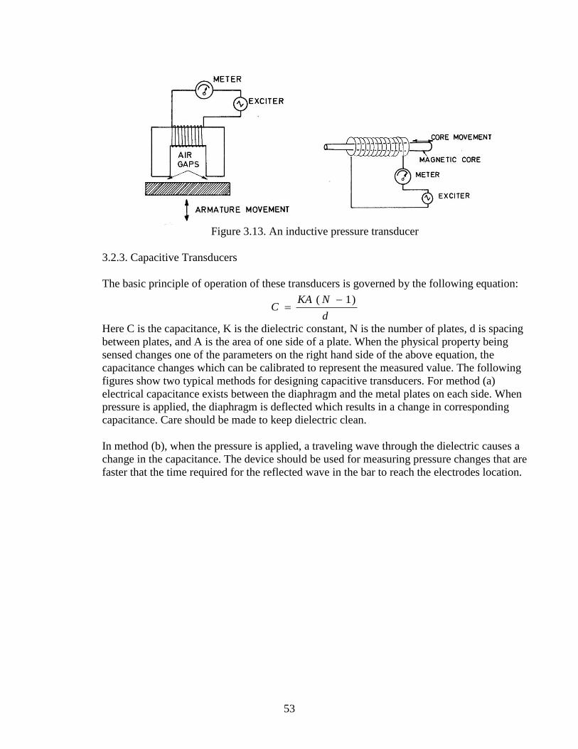
53

Figure 3.13. An inductive pressure transducer

3.2.3. Capacitive Transducers

The basic principle of operation of these transducers is governed by the following equation:

d

NKAC

)1(

Here C is the capacitance, K is the dielectric constant, N is the number of plates, d is spacing

between plates, and A is the area of one side of a plate. When the physical property being

sensed changes one of the parameters on the right hand side of the above equation, the

capacitance changes which can be calibrated to represent the measured value. The following

figures show two typical methods for designing capacitive transducers. For method (a)

electrical capacitance exists between the diaphragm and the metal plates on each side. When

pressure is applied, the diaphragm is deflected which results in a change in corresponding

capacitance. Care should be made to keep dielectric clean.

In method (b), when the pressure is applied, a traveling wave through the dielectric causes a

change in the capacitance. The device should be used for measuring pressure changes that are

faster that the time required for the reflected wave in the bar to reach the electrodes location.

54

(a) (b)

Figure 3.14. Examples of capacitive transducers.

55

Chapter 4

4

PRESSURE PROBES FOR FLUID

VELOCITY AND VOLUME

MEASUREMENTS

56

4.0. PRESSURE PROBES FOR FLUID VELOCITY MEASUREMENTS

4.1. Pitot Tube

In 1732, Henri Pitot offered the first description of a tube that was used to measure mean

velocity in a river and for this reason the pitot tube is named after him. Generally pitot tubes are

classified according to the quantities that they measure. The word pitot tube refers to a

cylindrical tube with its open end pointed upstream opposite to the flow direction which

measures impact or total pressure. Another type is pitot static tube which is two concentric tubes

that measure both static and total pressures. The difference between the two pressures are used to

obtain the mean velocity.

When total pressure alone is measured, local wall static pressure from static pressure hole is used

to obtain the pressure differential for calculation of the mean velocity.

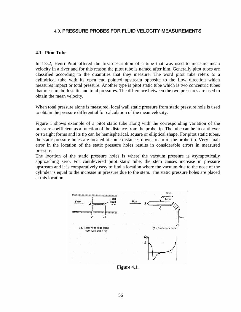
Figure 1 shows example of a pitot static tube along with the corresponding variation of the

pressure coefficient as a function of the distance from the probe tip. The tube can be in cantilever

or straight forms and its tip can be hemispherical, square or elliptical shape. For pitot static tubes,

the static pressure holes are located at some distances downstream of the probe tip. Very small

error in the location of the static pressure holes results in considerable errors in measured

pressure.

The location of the static pressure holes is where the vacuum pressure is asymptotically

approaching zero. For cantilevered pitot static tube, the stem causes increase in pressure

upstream and it is comparatively easy to find a location where the vacuum due to the nose of the

cylinder is equal to the increase in pressure due to the stem. The static pressure holes are placed

at this location.

Figure 4.1.

57

If D is the diameter of the cylinder, d1 and d

2 are respectively the diameters of total and static

pressure holes, and 1and

2 are respectively the distances between the nose and static pressure

holes and the static pressure holes and the stem, Prandtl offers the following criteria for

designing a pitot static tubes:

1

2

1

2

3

8 1 0

0 3

0 1

D

D

d D

d D

.

.

(8 holes equally spaced)

Some other designers have used 8D and 16D for respectively 1 and

2.

Assuming there is no significant variation in the mean velocity across the nose of the tube, the

Bernoulli's equation for one dimensional flow is used to obtain the mean velocity from pressure

differential. For steady flow, along a streamline, the Euler's equation can be written as:

d pg d Z d V

1

20

2

Here d p is the pressure difference, is the fluid density, g is the acceleration of gravity, dZ

is elevation difference and V is fluid velocity along the streamline. Integration of above

equation leads to:

pg Z V

1

2

2C o n s ta n t

If flow is incompressible ( is constant) and variation in potential energy is insignificant, and

knowing that velocity is zero at the surface, then we have:

p p Vt s

1

2

2

Here pt and p

s are respectively the total and static pressures.

Pitot tube nose geometry should be such that it does not deflect the streamlines and causes flow

separations. The size of the tube introduces errors in the measurements. When the local pressure

in the vicinity of a body is reduced significantly, cavitation occurs. For a pitot tube, the

occurrence of cavitation beyond the tip does not change total pressure reading. However, for

pitot static tube, the presence of cavitation results in appreciable change in static pressure

measurement.

An error of 2% in measured pressure is introduced if the Reynolds number based on tube

diameter is higher than 300.

58

Static pressure holes are used for surface pressure measurements. From various experiments,

accurate static pressure measurements are obtained if the hole is perpendicular to the surface and

if its diameter is around 0.25 mm. If the hole diameter is 1mm or if it is off by as much as 45

degrees from the perpendicular line, an error equal to 1% of the dynamic pressure is introduce in

the measurements.

In a two dimensional flow field, a two dimensional probe measures average magnitude and

direction of the velocity in a small area rather than at a point. The effective center, yc of total

pressure of a square ended circular impact tube is given by Young and Mass (1936) as:

y

D

d

D

c 0 1 3 1 0 8 2

1. .

Results of Hemke (1926) shows that if the total pressure hole is less than or about 0.15 mm,

accurate pressure measurements are obtained.

For tubes used in a rake, results of Krause (1951) show that correct static pressure measurements

can be obtained if the center distance between heads is greater than 6 head diameter. However, if

the Mach number is greater than 0.6, greater distance is required.

4.1.1. Yaw Angle Sensitivity and Tube Inlet Geometry

The impact pressure is very sensitive to the yaw angle. In order to have a probe which is

insensitive to the angularity, a shielded total pressure probe known as a Kiel probe is used.

Figure 2 shows a Kiel probe. Results of Gracey et al (1951) show that the total pressure from kiel

probe is insensitive to the angularity up to Mach number 0.3 and then decreases with increasing

Mach number. Those probes with curved entry have less sensitivity to the angularity than those

who have straight conical entry. Figure 2 also shows a minimum type probe proposed by

markowski and Moffat (1948) which is used to obtain total pressure in turbomachinary.

59

Figure 4.2

Dudziniski and Krause (1971) studied the effects of inlet tube geometry of miniature total

pressure tubes on pressure measurements. Their studies are limited to five inlet geometry of

circular, flattened oval and internal bevel at 15, 30, and 45 degrees. Tables 1 and 2 show the tube

tested and their dimensions. Testing criteria is that up to what flow angle there is only 1% error

in the total pressure as compared to the impact pressure. The tubes are tested in air in the Mach

number range of 0.3 to 0.9 and Reynolds numbers of 500 to 80,000. The flow angle is changed

between -45 degrees and 45 degrees. Their results show that the internally beveled tube with 15

degrees bevel angle has the highest flow angle ( 2 7 ) for producing accurate total pressure. The

flow angle decreases with increasing the bevel angle. Minimum flow angle of 12 degrees is

obtained for the flattened oval geometry.

60

Tables 4.1 and 4.2.

61

4.1.2. Turbulence Effects

Generally turbulence in a fluid stream causes a pressure reading that is higher than the true

pressure. Goldstein (1936) offers the following expressions for true total ( )Pt

and static ( )Ps

pressures in isotropic turbulent flow:

P Pq q

t tm e a s u r e d

2 2

2 2

P Pq

s sm e a s u r e d

2

6

Here, q q an d are respectively mean and fluctuating components of measured velocity.

In a pipe flow, based on experimental results of Townsend (1932), Fage (1936) offer the

following expressions for obtaining true static pressure:

P Pq

s sm e a s u r e d

2

4

Christiansen and Bradshaw (1981) studied the effects of free stream turbulence intensity of 24

percent, on the mean pressure coefficients of several static pressure probe and yaw meter, for a

range of yaw angles and ratios of tube size to typical eddy size. The probes tested are shown in

Figure 3 are a standard static pressure probe, a disc static pressure probe, a Conrad three-hole

yaw meter, a Gupta three hole yaw meter, and a single hole yaw meter.

62

Figure 4.3

Their results show that the multi-hole pressure probe yaw meters are not much affected by the

ratio of the eddy size to the probe size. However, the effects of free stream turbulence can

become large if the instantaneous yaw angle is larger than 10 degrees. The yaw angle calibration

in free stream turbulence shows significant difference from the corresponding results for the

laminar free stream beyond this value.

The turbulence effect on readings of Gupta probe was much severe than others. Their overall

results show that the yaw meter probes are excellent device for obtaining the mean pressure

coefficient, especially if they are used as a null reading devices.

The disc static pressure probe was sensitive to the flow angles and the free stream turbulence.

Small flow angles and free stream turbulence caused significant change in its calibration and it

was recommended not to use this probe in turbulent flow.

For standard static pressure probe, results show that the variation of the static pressure

coefficient with eddy size was significant. However, the error caused due to the presence of free

stream turbulence for the range of ratios of tube size to eddy size investigated, was about 2

percent of the dynamic pressure.

4.1.3 Measurement at Low Reynolds Number

The accuracy of the total pressure tube is not only depends on the geometry of the tube and the

impact opening but also depends on Reynolds number based on tube external head diameter. For

Reynolds number less than 500, the magnitude of the pressure coefficient define as:

63

CP P

U

i

i

1

2

2

becomes increasingly higher than unity with decreasing Reynolds number. Here P Pi an d

are

respectively impact and free stream static pressures and U

is the free stream mean velocity.

Table 3 (Folsom (1956)) gives theoretical pressure coefficient for impact tubes with different

probe head shapes at low Reynolds numbers.

Table 4.3

4.1.4 Measurements in Supersonic Flows

In supersonic flow the pitot static tube is usually a cone-cylinder type with 15 degrees total

included angle with static holes are located about 13 tube outside diameter downstream of the

cone base. Results of the experiments show that for Reynolds numbers based on tube outside

diameter of higher than 3500, accurate static and total pressure measurements are obtained.

Some results show that the accuracy decreases with decreasing Reynolds number.

4.2 Five Holes Probe

64

Five hole probes are mostly used to obtain the components of the mean velocity vector in a three

dimensional flow field. As pointed out by Treaster and Yocum (1979), the first application of the

five hole probe dates back to 1915 by Taylor and followed by Pien (1958) who found that a set

of calibration charts are necessary before the probe can be used in any experiments. Figure 4

shows a five hole probe along with the corresponding equations for obtaining mean velocity

components. Depending on the mode of calibration, the equations for obtaining the velocity

vectors are different. The main idea is to use the right equations for obtaining the mean velocity

components.

Figure 4.4.

Based on the geometry shown, for obtaining the calibration charts, the pressure coefficients and

average pressure are defined as:

CP P

P Pp

y a w

2 3

1

CP P

P Pp

p itc h

4 5

1

CP P

P Pp

to ta l

to ta l

1

1

CP P

P Pp

s ta tic

ya w

1

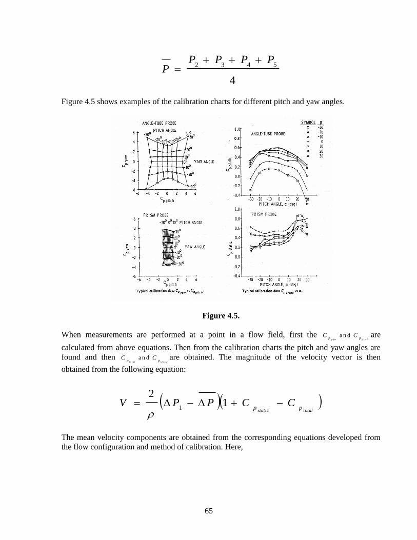
65

PP P P P

2 3 4 5

4

Figure 4.5 shows examples of the calibration charts for different pitch and yaw angles.

Figure 4.5.

When measurements are performed at a point in a flow field, first the C Cp p

y a w p itc h

a n d are

calculated from above equations. Then from the calibration charts the pitch and yaw angles are

found and then C Cp p

to ta l s ta tic

a n d are obtained. The magnitude of the velocity vector is then

obtained from the following equation:

totalstatic

ppCCPPV 1

2

1

The mean velocity components are obtained from the corresponding equations developed from

the flow configuration and method of calibration. Here,

66

P P P

PP P P P

re f1 1

2 3 4 5

4

a n d

For obtaining the three components of the mean velocity in low speed flows, Ligrani et al (1989)

presents description along with calibration charts for a miniature five hole pressure probe. Their

results compared well with the corresponding results from a Kiel probe in a curved channel.

Measurements of Treaster and Yocum (1979) show week dependency of Cp

s ta t ic on flow

Reynolds number and dependency of C Cp p

y a w s ta tic

a n d on the distance between the probe and

the wall. The Reynolds number dependency can be avoided if the calibration charts are obtained

at or in the range of Reynolds numbers that the experiments are performed.

When the center hole of the probe is within two probe diameters from the wall and is outside the

boundary layer, the measured pressure coefficients are inaccurate. However, when the probe is

used for measurements in boundary layers, the main errors are due to the spacing between the

probe off center pressure taps and the presence of the velocity gradient upstream of the probe.

All measured pressures from off center pressure taps and resulting velocity components should

be corrected for the corresponding pressure or velocity gradient in spanwise and vertical

directions (i.e. Sitaram et al (1981), Eibeck and Eaton (1985), and Westphal et al (1987)). The

procedure may be to subtract addition of the mean velocity components due to the velocity

gradient upstream of the probe from the corresponding measured values.

Another approach for correcting for spatial resolution and downwash velocity for multiple-hole

probes is given by Ligrani et al (1989) where for pressure corrections, cubic spline curves are fit

to the measured pressures at different spanwise but constant vertical locations and then the

values of off center pressure taps are corrected by interpolating them to the center pressure hole

location. For correcting velocity components in spanwise and vertical directions, addition of

velocity gradient in corresponding direction multiplied by a constant is proposed. In their case

which was measurements in a curved channel flow, the constant was 20% of the probe diameter.

Westphal et al (1987) from calibration results of Treaster and Yocum (1979) show that for

variation in pitch and yaw angles of 20 degrees, C Cp p

y a w p itc h

a n d are nearly independent of

pitch and yaw angles respectively and it is possible to express variation of these coefficients with

respectively yaw and pitch angles in terms of polynomials. This approach is preferred in flow

configurations where the flow angle does not go beyond 20 degrees.

Huffman et al (1980) used slender body theory to obtain theoretical relationships for variation in

average, pitch, yaw, static and total pressure coefficients for a conical probe. Figure 6 shows

67

their probe configuration and dimensions. Their theoretical results for average pressure

coefficient compares well with the corresponding experimental results up to Mach number 0.9.

The theoretical calibration charts for the variation in C Cp p

y a w p itc h

a n d with pitch and yaw angles

also have similar characteristics as the corresponding experimental results. However, the theory

becomes incapable of predicting correct calibration charts for pitch and yaw angles beyond 20

degrees.

Figure 4.6. In order to increase the range of flow angles for the five hole probes, Ostowari and Wentz

(1983) present new calibration approach by replacing the center pressure tap with the upwind

port pressure as the reference total pressure and the stalled downwind pressure tap with the

center pressure tap. Figure 7 shows their five tube probe. This approach extends the calibration

range for the pitch angles while the yaw angle remains in null position. Their results show good

calibration curves up to the flow angles of 85 degrees.

4.3. Preston Tube

Prston (1954) based on the law of the wall proposed a method for determining the wall

shear stress and subsequently the skin friction coefficient in boundary layers. His method was

based on measuring the total pressure by placing a pitot tube on the surface and the static

pressure which is measured on the surface at the same location. In non-dimensional form the

pressure difference is related to the friction velocity ( )U

and subsequently the wall shear stress

as:

dUf

U

P

2

68

Figure 4.7.

Near the surface, the boundary layer thickness depends on the wall shear stress,

, density of

the fluid, , kinematics viscosity, , and a length scale. For a pipe flow Preston proposed the

following relation between the wall shear stress and the measured dynamic pressure:

2

2

0

2

2

44d

PPf

dw

Here, P Pw0

an d are respectively total and wall static pressures and d is the diameter of the pitot

tube. From measurements of flow through pipes, he found the following relationship between the

measured pressure and the wall shear stress:

2

0

102

2

10

4log

8

7628.2

4log

dPPdw

Patel(1964) performed calibration of the preston tube in three different pipes using fourteen

different pitot tubes for three cases of zero, adverse and favorable pressure gradients. His results

show that the calibration results of Preston are not very accurate. Using McMillan relation for

effective center of the pitot tube defined as y K d1

2 where in the sublayer region K is defined

as 0.3, he offered the following equations for the case of Zero pressure gradient:

69

in linear sublayer:

4.1for 2

1log

2

1

2

1 *2

10

**

yKxy

in transition region:

3.56<4.1for

2

10log

2

log2

*

2

1

1010

**

*

y

BCK

Ayx

y

and finally in the fully developed turbulent region

*

10

*

1010

**

56.3for

2

log2log

22

log2

y

BKy

Ayx

The constants A and B are determined to be 5.5 and 5.45 respectively. The expressions for

x y* *a n d are:

2

2

10

*

2

2

0

10

*

4log

4log

d

x

dPPy

w

In transition region the constant C is difficult to determined and instead the following cubic

polynomial used:

y x x x* * * *

. . . . 0 8287 0 1381 0 1437 0 0062 3

Preston also offered the same equation for the range 1 5 3 5. .*

y .

70

Patel also showed that in the case of adverse pressure gradient, large diameter preston tube

register larger errors and in the case of favorable pressure gradient the preston tube register

nearly correct readings. Since for large pressure gradient, departure from the law of the wall is

seen, he offered the following restrictions in obtaining the wall shear stress using the Preston

tube:

i) Adverse Pressure Gradient

250 ,015.00

6%error maximum

200 ,01.00

3%error maximum

dU

dU

ii) Favorable pressure gradient

250 ,007.00

6%error maximum

200 ,005.00

3%error maximum

dU

dU

Here which is obtained from dimensional analysis defined as

U

d P

d x3 .

71

4.3. Volume Flow Measurements

4.3.1. The Venturi Meter

The venturi meter uses reduction in area and the resulting changes in pressure to measure the

volume or mass flow passing through the tube. Figure 8 shows two design consideration, one for

inline continuous measurements and the other using a bypass valve for periodic monitoring of

the flow volume. The pressure taps placed upstream and downstream of the venturi are used for

pressure measurements.

)(2

**212

PPg

AMCQc

a

2

1

2

1

2

I

a

A

A-1factorApproach ofVelocity M

Flow Volumetric Ideal

Flow Volumetric Actual

Q

QtCoefficien Discharge

Flow Volumetric Actual

C

Qa

Figure 4.8. The venturi meter and its set-up design.

72

2.2 The Orifice Plate

The orifice plate is used for differential pressure measurements. It is used for both liquid and gas

applications. The differential pressure between upstream and downstream sides of the orifice

plate is measured using pressure taps located on the corresponding sides. The pressure taps

should be located far enough from the orifice plate where there is no flow recirculation.

)(2

212PP

gKAQ

c

a

tCoefficien Flow

Flow Volumetric Actual

K

Qa

Figure 4.9. The orifice plate and its flow configuration.

4.3.2. Rotometers (variable Area Meter)

The position of the float or Bob is as a result of a balance between the drag force on Bob and

Bob’s weight and the buoyancy force. The position can be calibrated to show mean velocity,m

U ,

volume flow rate, Q , or mass flow rate, m .

Taking D= diameter of the tube at inlet, d=diameter of Bob, C= meter’s constant (found through

calibration), BB,

V and A , ,fB

are respectively the density of the Bob, fluid density, projected

area and the volume of the Bob, The equations for m

U , Q , and m are:

73

2/1

22

2/1

)(

)(4

where,

2

ffB

m

f

fB

BD

B

m

CZm

dZDAAUQ

AC

gVU

Here D

C and are respectively the drag coefficient of Bob and a correction parameter related

to the tube taper.

Figure 4.9. The Rotameter (the Variable Area Meter)

4.3.4. Doppler Flowmeter (Meters Liquids in Pipe Flow)

It is used for measuring mass flow rate, volume flow rate and/or mean flow velocity.

74

An ultrasonic beam from the piezoelectric crystal is transmitted through the pipe wall into the

fluid at an angle to the flow stream. Reflected signals of the flow disturbances are detected by a

second piezoelectric crystal. The two signals are compared and their differences are calibrated to

indicate the required measurement.

Limitations:

Pipe wall thickness should be less than 1.92 cm.

Liquid mean velocity should be higher than 0.15 m/sec.

The metered liquid should have at least 2% suspended solids by volume.

Pipe material should be homogeneous composition (For example it can not be used for

concrete or composite pipes).

Figure 4.10. The Doppler Flowmeter

75

References

Cheremisinoff, N.P., Applied Fluid Flow Measurement, fundamentals and technology, 1979,

Marcel Dekker, INC, New York.

Christiansen, T. and Bradshaw, P., 1981, ``Effect of Turbulence on Pressure probe,” J. Phys. E.:

Sci. Instrum., Vol. 14, pp.992-997.

Eibeck, P.A., and Eaton, J.K., 1985, ``An Experimental Investigation of the Heat Transfer

Effects of a Longitudinal Vortex Embedded in a Turbulent Boundary Layer,” Report MD-48,

Mechanical Engineering Department, Stanford University, Stanford, California.

Fage, A., 1936, ``On the Static Pressure in Fully-Developed Turbulent Flow,” Proceedings of the

Royal Society of London, Series A., Vol. 155, pp. 576-596.

Folsom, R.G., 1956, ``Review of the Pitot Tube,” Transaction of the ASME, pp. 1447-1460.

Fox, R.W., and McDonald, A.T., Introduction to Fluid Mechanics, Fourth Edition, Wiley, 1992.

Goldstein, S., 1936, `` A Note on Measurement of Total Head and Static Pressure in a Turbulent

Stream,” Proceedings of the Royal Society of London, Series A., Vol. 155, pp. 570-575.

Gracey, W., Letko, W., and Russel, W.R., 1951, ``Wind Tunnel Investigation of a Number of

Total Pressure Tubes at High Angles of Attack-Subsonic Speeds,” NACA TN 2331.

Hemke, P.E., 1926, ``Influence of the Orifice on Measured Pressures,” NACA TN 250.

Huffman, G.D., Rabe, D.C., and Poti, N.D., 1980, ``Flow Direction Probes From a Theoretical

Point of View,” J. Phys. E.: Sci. Instrum. Vol. 13, pp. 751-760.

Krause, L.N., 1951, ``Effects of Pressure-Rake Design Parameters on Static Pressure

Measurement for Rakes Used in Subsonic Free Jet,” NACA TN 2520.

Ligrani, P.M., Singer, B.A., and Baun, L.R., 1989, ``Spatial Resolution and Downwash Velocity

Corrections for Multiple-Hole Pressure Probes in Complex Flows,” Experiments in Fluids, Vol.

7, pp. 424-426.

Markowski, S.J., and Moffatt, F.M, 1948, ``Instrumentation for Development of Aircraft Power

Plant Components Involving Fluid Flow,” Trans. SAE, Vol. 2, pp. 104-116.

Patel, V.C., 1965, ``Calibration of the Preston Tube and Limitations on Its Use in Pressure

Gradients,” J. Fluid Mech. Vol. 23, Part 1, pp. 185-208.

Pien, P.C., 1958, ``Five-Hole Spherical Pitot Tube,” David Taylor Model Basin Report 1229.

76

Preston, J.H., 1954, ``The Determiation of Turbulent Skin Friction by Means of Pitot Tubes,” J.

Roy. Aero. Soc. 58,109.

Sitaram, N., Lakshminarayana, B., and Ravindranath, A., 1981, ``Conventional Probes for the

Relative Flow Measurement in a Turbomachinary Rotor Blade Passage,” Transactions of the

ASME, Vol. 103, pp. 406-414.

Treaster, A.L., and Yocum, A.M., 1979, ``The Calibration and Application of Five-Hole Probes,

” ISA Transactions, Vol. 18, No.3, pp. 23-34.

Townsend, H., 1934, ``Statistical Measurements of Turbulence in the Flow of Air Through a

Pipe,” Proceedings of the Royal Society of London, Series A., Vol. 145, pp. 180-211.

Westphal, R., Pauley, W.R., and Eaton, J.K.,1987, ``Interaction Between a Vortex and a

Turbulent Boundary Layer, Part I: Mean Flow Evolution and Turbulence Properties,” NASA TM

88361.

Young, A.D., Mass, J.N., 1936, ``The Behaviour of a Pitot Tube in a Transverse Total-Pressure

Gradient,” British ARC, R & M 1770.

77

Chapter 5

5

TEMPERATURE MEASUREMENTS_____ Compiled and written by: Huy Hoang, Ph.D.

78

Temperature measurements have countless applications in the world today. Typical examples of application ranges from the thermostat controlled temperature for the air conditioning inside the house during the summer season to the heat rejection of a spacecraft in space.

Temperature of an object is defined as a measure of thermal potential of that object. It cannot be measured by using basic standard methods for direct comparison. It can only be determined through the some standardized form of calibrated devices. Various instruments have been developed for different applications of temperature measurement. The basic operations of these instruments are designed to accompany its primary effects of temperature change. The effects include the changes in physical state, in chemical state, electrical properties, mechanical properties, and optical properties of thermometers.

I. Liquid-in-Glass Thermometers

Mercury-in-glass thermometer is an example of liquid filled thermometer. The thermometer consists of a relative large bulb at the lower end, a capillary tube with scale, and mercury filling both the bulb and a portion of the capillary as shown in Figure 1. The volume enclosed in the capillary above the liquid may contain a vacuum or be filled with air or inert gas. As the temperature is raised, the expansion of the mercury causes it to rise in the capillary of the thermometer. The height of the rise is used as a measure of the temperature. By calibrating the expansion of the mercury at different temperature, the thermometer can provide accurate temperature reading.

Figure 1. Mercury-in-glass thermometer There are several desirable properties for liquid-in-glass thermometer. These

properties include: 1. The relationship between temperature and dimensional change should be

linear.

79

2. The liquid should have a coefficient of expansion as large as possible. Large coefficient of expansion makes possible larger capillary bores and easier reading. The coefficient of expansion for alcohol is larger than mercury.

3. The liquid should operate in a reasonable temperature range without change of state. Mercury is limited at the low-temperature end by its freezing point, -39ºC, and at the high-temperature end at its boiling point, 357ºC. Alcohol is limited at the low-temperature end by its freezing point, -75ºC, and at the high-temperature end at its boiling point, 127ºC.

4. The liquid should be safe to human health and environments. Mercury has very high toxicity and chemical hazardous. For this reason, alcohol filled thermometer is the preferable device.

II. Thermocouples

A thermocouple consists of two wires of dissimilar metals coupled at the probe tip (sensing/or measuring junction) and extended to the reference junction of known temperature. When the probe tip is heated, the temperature difference between the sensing junction and the reference junction is measured the change in voltage at the reference junction. The change in voltage is caused by the Seebeck effect named after Thomas Seebeck discovered this phenomenon in1821. The temperature gradients along the conductors between the two junctions generate a small voltage which is known as the Peltier electromotive force (e.m.f). The voltage is usually measured in milivolts (1/1000th of Volt). The thermocouple wires are chosen according to the maximum temperature measurement and linearity of its output (e.m.f) versus temperature.

Figure 2. Thermocouple circuit and probe Thermocouple Types There are several thermocouple types available for a wide range of temperature

from -250ºC to 3000ºC. Each type has a useful temperature range and sensitivity for different applications. American Society for Testing and Materials (ASTM), which is

80

recognized in the United States as the authority for temperature measurements, has established the guidelines for different thermocouple types. The ASTM E-230 guidelines cover the wire composition, color codes, and manufacturing specifications.

Commercial thermometers are specified by Instrument Society of America (ISA) types. The ISA types are recognized by the letter designations. Thermocouple with letter types E, J, K, R, and T are common used. Type E, J, K, N and T are base metal thermocouples and can be used up to 1000C. Base metal thermocouples compose of common and inexpensive metal wires such as nickel, iron, and copper. Type S, R, and B are noble-metal thermometer and can be used up to about 2000C. Noble metal thermocouples are manufactured with precious metal wires of Platinum and Rhodium. Type C is refractory metal thermocouple and can be used up to 2320C. Refractory metal thermocouples are very expensive, difficult to manufacture, and wires made from the exotic and brittle metals like tungsten and Rhenium.

The following table summarizes the basic properties of different thermocouple types. Each manufacturer has its own thermocouple’s specifications.

Table 1. Different thermocouple types.

81

Conversion of Voltage to Temperature The measured voltage that a thermocouple produces can be converted to

temperature. The voltage and temperature are not quite linear regression of the first-order. A polynomial equation that best describes the relationship between the voltage (V) versus temperature (T) for a wide range of temperature is:

n

n

n

Nn

n

nVaVaVaaVaT

..2

210

0

A typical coefficient for thermocouple types E, J, K, R, S and T is listed the Table 2.

Table 2. Coefficients of polynomial equation for voltage to temperature conversion.

Measuring Junction Types Figure 3 shows the layout of measuring junction types. The choice of measuring

junction types depends on the application. Generally, the grounded junction offers the best compromise between performance and reliability.

Bare wire (exposed) junction provides the fastest response time but leaves the thermocouple wires unprotected against corrosion or mechanical damage.

82

Insulated (ungrounded) junction provides the protection for thermocouple junction and avoids the ground loops between instruments, power supplies, and sensors. The lead wire is fully insulated from the shield. The insulated junction is excellent for applications where stray electromotive forces would affect the reading and for rapid temperature cycling. Response time is slow due to insulation.

Grounded junction provides very fast response time approach of the bare wire junction. The shield and the lead wires are welded together, forming a complete shield and integrated junction. The grounded junction is recommended for applications with the presence of liquids, moisture, gas, or high pressure.

Figure 3. Layout of measuring junction types

III. Thermistors A thermistor is a thermally sensitive variable resistor which is made from semi-

conducting material. It has a very fast non-linear response to the temperature change and the majority of the thermistors has negative response coefficients due to their resistances decrease with increasing temperature. It is used widely in the laser diode and detector cooling applications because of their high sensitivity, small size, fast response times, and low cost. A thermistor is usually restricted to a temperature range of -100°C to 250° C. Figure 4 shows typical thermistor sensors and probes.

83

Figure 4. Typical thermistor sensors and probes. The resistance-temperature characteristics for most thermistors are described by

the Steinhart-Hart equation:

3)(ln*)(ln*

1RCRBA

T

where T is the absolute temperature (in Kelvin), R is the resistance in Ohm, and A, B, and C are constants which can be determined from measured values of resistance and temperature. Typical resistance-temperature response curves are shown in Figure 5. For good calibration data, the Steinhart-Hart equation introduces errors of less than 0.1°C over a temperature range of -30°C to 150°C.

.

84

Figure 5. Resistance-Temperature response curves

IV. Resistance Thermometers

Resistance temperature detector (RTD) contains a resistor that changes the resistance value as its temperature change. Unlike the thermistor uses ceramic semiconducting materials which response inversely with temperature, the RTD probe has the resistance increase with temperature. RTD is available in a tube and wire and mineral construction. The platinum resistance thermometer is a common device of the RTD. It consists of a length of platinum which has been trimmed in length to give an accurate resistance of 100 at 0 C. The wire is wounded and protected with insulation. It is then further protected with a metallic shell. The resistance changes with a change in temperature. It provides a nearly linear temperature resistance relationship which is stable over a long time period. Its thermal response suffers due to degree of mechanical protection. Platinum resistance thermometer is typically used for temperature sensitivity and laboratory applications.

85

Figure 6. Platinum resistance thermometer

V. Bi-metal Thermometer The bi-metal thermometer consists of two thin metal strips with different

coefficient of linear expansions that are fastened together. The result is a strip that bends significantly when heated. One end of the strip is fixed and the other end is connected to a pointer on a calibrated dial that deflects with changes in temperature. When the strip is formed into a coil, its sensitivity is increased.

Figure 7. Bi-metal Thermometer Bi-metal thermometers are used in industrial process, food processing and waste

water. A typical bi-metal thermometer has maximum pressure of 125 psi (861 KPa) and the ambient operating conditions from -50°C to 120°C. The selection of bi-metal thermometer is based on the media and the ambient operation conditions. The bimetal should not expose continuously to process temperature over 425°C.

86

VI. Pyrometers Pyrometer is a non-contacting thermometer device to measure temperature in

the form of thermal radiation. Figure 8 shows a typical pyrometer instrument. There are three different instruments referred to as pyrometers: total radiation, the optical, and the infrared pyrometers.

Figure 8. A typical pyrometer instrument The total radiation pyrometer has a thermal sensor that infers the temperature of an object by detecting its naturally emitted thermal radiation. The optical pyrometer collects the visible and infrared energy from an object and focuses through lenses on a detector. The infrared pyrometer is similar to the total radiation except that the

measurements are restricted to the infrared spectrum from 0.7 to 1000m wavelengths. The detectors of pyrometers convert the collected radiation energy into an electrical signal to drive a temperature display as shown in Figure 9.

Figure 9. Infrared measuring system pyrometer.

87

The pyrometers offer the following advantages:

1. It is very fast and time savings. 2. Measurements can be taken for very high temperature or high voltage objects

without in contact with them. Typical applications are the temperature measurements for the molten glass or molten metal during the smelting and forming operations.

3. Measurements can be taken for moving target or object. 4. There is no energy lost or interference between the instrument and the object. 5. There is no hazardous risk or contamination on the surface of the object.

THERMAL RESPONSE The most important characteristic for selecting a thermometer for a particular application is its thermal response. The thermal response is defined by the time it takes to change 63.2% of the step change. This is defined as the “time constant” and is irrespective of the step change in temperature. Figure 10 shows a temperature-time plot for a thermometer with two different step changes. The time constant remains the same, irrespective of the difference in temperature step changes.

Figure 10. Time constant

88

References

1. http://dtec.net.au/Thermocouple%20Probes,%20EGT%20Exhaust%20Gas%20Temperature%20%E2%80%98pyro%E2%80%99,%20K%20type.htm

2. http://instrumentationandcontrollers.blogspot.com/2010/06/thermocouple-with-circuit.html

3. Thermocouple_Theory http://www.sensortecinc.com/docs/technical_resources/Thermocouple_Theory.pdf

4. Measuring Temperature with Thermocouple http://www.noise.physx.u-szeged.hu/digitalmeasurements/sensors/thermocouples.pdf

5. http://www.efunda.com/designstandards/sensors/thermocouples/thmcple_intro.cfm 6. http://www.accessscience.com/overflow.aspx?SearchInputText=Thermometer&ContentT

ypeSelect=10&term=Thermometer&rootID=797745 7. http://www.npl.co.uk/educate-explore/factsheets/temperature 8. http://www.winters.com/pdfs/Cut%20Sheets/Thermometer/BimetalThermometer.pdf 9. http://www.circletrack.com/chassistech/ctrp_0801_wheel_tire_products/photo_06.html 10. Principles of Non-contact Temperature Measurement

http://support.fluke.com/rayteksales/Download/Asset/IR_THEORY_55514_ENG_REVB_LR.PDF

11. http://www.globalspec.com/reference/10956/179909/chapter-7-temperature-measurement-radiation-pyrometers

12. http://www.efunda.com/designstandards/sensors/thermistors/thermistors_intro.cfm 13. http://assets.newport.com/webDocuments-EN/images/AN02_Select_Thermistor_IX.pdf 14. Beckwith, Thomas G. and Magrangoni, Roy D., Mechanical Measurements, 4th Edition,

Addison-Wesley Publishing,1990. 15. Rahai, Hamid R., MAE 300 Experiments, CSU Long Beach, CA. Spring 2011.

89

Chapter 6

6

DATA ACQUISITION Compiled and written by: Huy Hoang, Ph.D.

90

Data collection by hand for a single or multiple sample experiments is a tedious task and time consuming. In addition to the experiment uncertainties, human errors are difficult to avoid due to the lack of patience for doing the repetitive tasks. Also, some complex measurement tasks could not easily be done by hand. With the advance of modern technology, data can be easily recorded using automate systems with the use of personal computers (PC). Processed data can be display on the screen of computers instantaneously for most real time applications. The method of acquiring and recording data using computer controlled is called data acquisition. Data acquisition is a process of acquiring signals from a sensor, digitizing the signals with a data acquisition device, and application software. Figure 1 shows the schematic of data acquisition process. Figure 1, Schematic of data acquisition

1. Sensors A typical sensor used for acquiring signals from real world phenomena is a transducer. The transducer is a device that converts any measurement parameters from mechanical or electrical energy into electrical signals. For temperature measurements, a thermocouple produces a change in voltage emf between the sensing junction and the reference junction when it is heated up. The voltage is measured in milivolt (mV). For pressure and displacement measurement, a strain gauge is an example of resistance transducers that senses the strain produced by the forces applying on the wires of the gauge. The resistance is proportional to the change in the length of the wires and is measured in ohms.

Sensors

Data acquisition card

Computer with application software

Hardware drivers

Data acquisition storage

Application software program

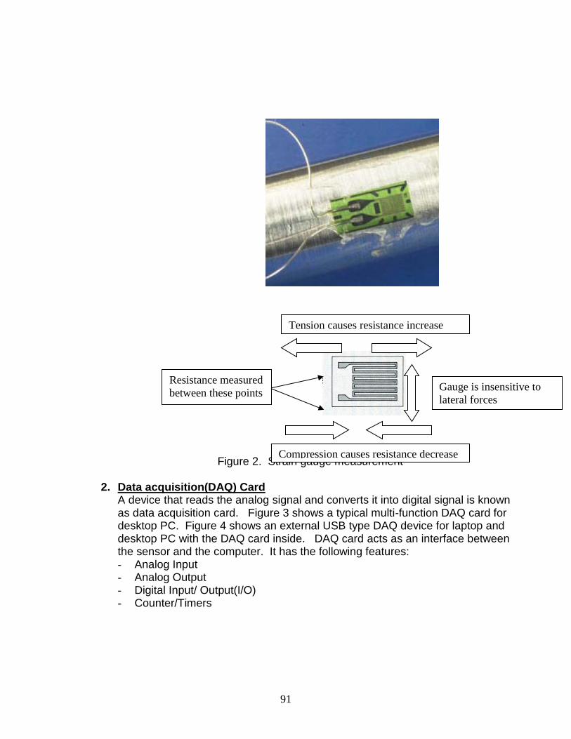
91

Figure 2. Strain gauge measurement

2. Data acquisition(DAQ) Card A device that reads the analog signal and converts it into digital signal is known as data acquisition card. Figure 3 shows a typical multi-function DAQ card for desktop PC. Figure 4 shows an external USB type DAQ device for laptop and desktop PC with the DAQ card inside. DAQ card acts as an interface between the sensor and the computer. It has the following features: - Analog Input - Analog Output - Digital Input/ Output(I/O) - Counter/Timers

Resistance measured

between these points

Compression causes resistance decrease

Gauge is insensitive to

lateral forces

Tension causes resistance increase

92

Figure 3. Multifunction data acquisition card ADLINK ACL-8112

Figure 4. NI USB-6008 DAQ device for laptop and desktop computer.

a. Analog Input An analog input is an input port to the DAQ card specifically for continuous, analog signals. Typical features of analog inputs are the number of channels, sampling rate, multiplexing, signal filtering, resolution, and input range.

Number of channels-This parameter specifies the number of channel inputs on boards of DAQ card. There are two types of channel inputs: single-end and differential. Single-ended inputs are used when the input signals are greater than 1V, the leads from the signal source to the analog input hardware are less than 15 ft, and all input signals share a common ground point. For differential inputs, each input has its own ground reference.

93

Sampling rate-The effective sampling rate is inversely proportional to the number of channels. A fast sampling rate acquires more input data points for a given time and can form a better representation of original signals.

Multiplexing-This is a common process when the DAQ card has to sample signals from many channels instead of one. The DAQ samples one channel at a time before switching to the next channel.

Signal filtering-The use of filtering is to remove the noise and unwanted signals.

Resolution-The number of bits to represent the analog signal is called a resolution. The higher the number of divisions of the input gives the higher the resolution of the signals

Input range- The electrical signals from the sensors or transducers must be optimized for the input ranges of the DAQ card. The low-level signals can be amplified to increase the resolution and to reduce noise.

b. Analog Output The measured electrical signal is often analog and must be converted into a digital signal so that it can be processed by a computer. The digital representation of an analog signal offers the following advantages: 1) digital signals can be stored and accessed in the computer RAM and hard

drive, 2) digital signals can be reproduced without errors. 3) digital signals can be imported or transferred between computers for processing and computational analysis. In general, the digital representation is not quite a good representation of the original analog data because the datum point between each digital sample is lost in the analog-to-digital conversion.

The process of analog-to-digital converter (ADC) is shown in Figure 5.

Figure 5. Analog-to-digital converter

94

Figure 6 shows a sine wave and its corresponding 3-bits digital image. A 3-bit ADC divides the analog range into 8 divisions. Each division is represented by a binary code between 000 and 111.

Figure 6. Digitized sine wave with a resolution of 3 bits

c. Digital I/O The use of digital I/O is to transfer the data between a computer and equipment such as data processors. The important parameters of digital I/O are the number of digital lines available, the rate at which the equipment can accepts, and the source and the drive capacity of digital lines.

d. Counter/timers The counter/timers circuitry is used for counting the occurrence of a digital event and generating the wave forms. The significant operations of counter/time are the resolution and clock frequency. The resolution is determined by the number of bits the counter uses. The clock frequency determines how fast the digital source input can be toggled.

3. Computer with application software Application software transforms the computer and data acquisition hardware into a complete data acquisition system for analysis and display. The driver software controls the functions of DAQ hardware such analog I/O, digital I/O, and counter/timers and manages the integration between the hardware and the computer. Labview and Matlab are the most common data acquisition software use world-wide by researchers and laboratories. The manufacturers of software provide DAQ drivers to integrate seamlessly with DAQ hardware, signal conditioning equipment, and the capability of computer operating system (OS). A display of data acquisition system with Labview is shown in Figure 7.

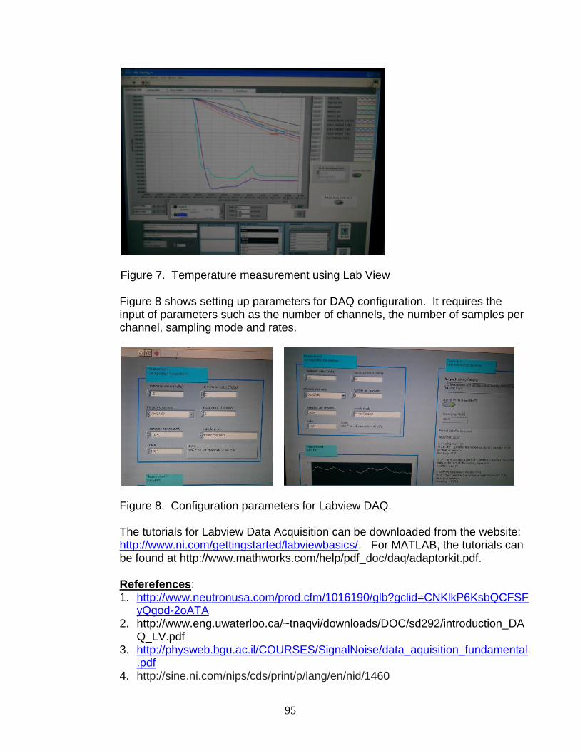
95

Figure 7. Temperature measurement using Lab View

Figure 8 shows setting up parameters for DAQ configuration. It requires the input of parameters such as the number of channels, the number of samples per channel, sampling mode and rates.

Figure 8. Configuration parameters for Labview DAQ.

The tutorials for Labview Data Acquisition can be downloaded from the website: http://www.ni.com/gettingstarted/labviewbasics/. For MATLAB, the tutorials can be found at http://www.mathworks.com/help/pdf_doc/daq/adaptorkit.pdf.

Referefences: 1. http://www.neutronusa.com/prod.cfm/1016190/glb?gclid=CNKlkP6KsbQCFSF

yQgod-2oATA 2. http://www.eng.uwaterloo.ca/~tnaqvi/downloads/DOC/sd292/introduction_DA

Q_LV.pdf 3. http://physweb.bgu.ac.il/COURSES/SignalNoise/data_aquisition_fundamental

.pdf 4. http://sine.ni.com/nips/cds/print/p/lang/en/nid/1460