Macroeconomic Modelling in EMU: How Relevant is the Change in Regime?

Electronic copy available at: http://ssrn.com/abstract=997219

Javier Andrés and Fernando Restoy

MACROECONOMIC MODELLINGIN EMU: HOW RELEVANTIS THE CHANGE IN REGIME?

2007

Documentos de Trabajo N.º 0718

Electronic copy available at: http://ssrn.com/abstract=997219

MACROECONOMIC MODELLING IN EMU: HOW RELEVANT IS THE CHANGE

IN REGIME?

MACROECONOMIC MODELLING IN EMU: HOW RELEVANT

IS THE CHANGE IN REGIME? (*)

Javier Andrés (**)

UNIVERSIDAD DE VALENCIA AND BANCO DE ESPAÑA

Fernando Restoy (***)

BANCO DE ESPAÑA

(*) We are grateful to Máximo Camacho, Juan Francisco Jimeno, Julio Segura, Frank Smets and an anonymous refereefor helpful comments. (**) E-mail: [email protected]. (***) E-mail: [email protected].

Documentos de Trabajo. N.º 0718

2007

The Working Paper Series seeks to disseminate original research in economics and finance. All papers have been anonymously refereed. By publishing these papers, the Banco de España aims to contribute to economic analysis and, in particular, to knowledge of the Spanish economy and its international environment. The opinions and analyses in the Working Paper Series are the responsibility of the authors and, therefore, do not necessarily coincide with those of the Banco de España or the Eurosystem. The Banco de España disseminates its main reports and most of its publications via the INTERNET at the following website: http://www.bde.es. Reproduction for educational and non-commercial purposes is permitted provided that the source is acknowledged. © BANCO DE ESPAÑA, Madrid, 2007 ISSN: 0213-2710 (print) ISSN: 1579-8666 (on line) Depósito legal: Unidad de Publicaciones, Banco de España

Abstract

We analyse the likely effects of changes in the monetary and financial regimes of EMU

countries on the dynamics of output and inflation. In particular, we evaluate the impact of

the regime shift on the forecasting performance of reduced-form models. Data for both the

pre-EMU and the EMU regimes are generated by a relatively standard open-economy-

DSGE model with sticky prices and wages, and restricted access to financial markets for

some individuals. We find that the effects of the shift in the monetary regime on the

processes followed by macroeconomic variables depend on the nature of the shocks

impacting the economy. For plausible shock distributions the reduction in the accuracy of

VAR-based inflation forecasts is relatively large and significant. The effect of the regime shift

on output forecasts seems rather more modest and statistically insignificant. The impact on

ouput forecasting accuracy would be comparatively much larger if the new monetary union

regime were accompanied by a moderate relaxation of constraints affecting financial

market access.

JEL codes: E17, E32, E37

Keywords: Forecasting, General equilibrium models, Monetary Union, Inflation and Output

dynamics.

1. Introduction

In the last few years, central banks and other policy institutions have shown anincreasing interest in Neo-Keynesian DSGE models (see e.g. Woodford’s 2003textbook) as a promising framework to conduct forecasting and policy analysis.This interest should come as no surprise. These models are micro-founded and, asthey assume sticky prices, allow nominal variables to play a relevant role. More-over, equilibrium conditions can be approximated by a set of explicit economicrelations that resemble those of traditional macro-models -albeit with fully en-dogenous expectational terms- in which parameters are deep in the sense of beingrelated to structural features of the economy. Last but not least, by exploitingoptimising conditions of a representative agent, this framework provides a usefuldevice to discuss optimal policy choices.The new models seem, in practice, quite suitable for analysing euro zone

economies1. As countries participating in EMU have experienced a sharp changein the rules governing interest rate decisions with respect to the previous regime,the presumption is that forecasts and policy simulations based on non-structuralmodels will be heavily flawed as a consequence of their substantive exposure tothe Lucas critique (Lucas, 1976). Only with a large number of observations in thenew monetary union regime would those models be able to recover the forecastingability they may have had in the previous regime. By contrast, DSGE modelsneed much less information to accommodate changes in the monetary regime bymodifying the structural parameters which have been affected by the regime shift.However, the new-generation DSGE models are currently subject to intensive

scrutiny by the profession. So far, their forecasting ability does not seem generallysuperior to more traditional macro models2. This explains why, despite their manytheoretical shortcomings, many institutions continue using standard reduced-form

1The Eurosystem has already shown a keen interest in exploring the capabilities of new DSGEmodels.To our knowledge, at least the ECB and the National Central Banks of Germany, France,Italy, Finland and Spain already have or are currently developing DSGE models.

2There have recently been some interesting attempts to build a bridge between VAR andDSGE models using Bayesian techniques (see del Negro and Schorfeide, 2004 and 2005 and delNegro et al., 2005). This approach has already delivered some promising forecasting results bycombining the in-sample fit of VARs with the more robust and parsimonious parametrisation ofDSGE models.

2

BANCO DE ESPAÑA 9 DOCUMENTO DE TRABAJO N.º 0718

models in their forecasting exercises. Along the same lines, some central banks(see Bank of England, 2005) have already constructed hybrid models with a coremicro-founded part and a number of more ad-hoc components that help to improvethe forecasting performance.Arguably, this suboptimal forecasting performance of DSGE models is partly

due to the lack of empirical relevance of some of their theoretical advantages. Mostresearchers would agree that major changes in the so-called deep or structuralparameters in an economy might have significant effects on the dynamics of outputand inflation. But it is also true that these kinds of developments are unusual,and that policy changes of a more limited scope are likely to have a meagre,hardly noticeable, effect. Along these lines Taylor (1989, 1999), Estrella andFuhrer (1998) and Rudebusch, (2005), among others, have argued that plausiblevariations in monetary policy rules do not change actual macroeconomic dynamicsin a statistically and/or economically significant manner3. These authors havefocused their analysis on the effects of changes in the estimated rules followed bythe Fed in the last third of the previous century on the stability of standard VARmodels.The issue remains open, however as to whether the negative results on the

relevance of the Lucas critique found for the US apply also to a deeper regimeshift such as the creation of a monetary union in Europe. This implies a potentiallylarge transformation as a result of the elimination of exchange rate fluctuationsacross member countries and the adoption of a brand-new common monetarypolicy for all of them.An additional element to be taken into account is that, in conjunction with

EMUmembership, most euro-zone economies have experienced other major struc-tural transformations that are only partially linked to euro adoption. In partic-ular, households’ balance sheets have changed markedly in several countries as aconsequence of the consolidation of an environment of macroeconomic stability,lower financing costs, and increased flexibility and competition in the financialsector. Those developments are also likely to influence the monetary transmissionmechanism and, therefore, the dynamics of macroeconomic variables in a relevant

3See Lindé (2001) as an example of the opposite view.

3

BANCO DE ESPAÑA 10 DOCUMENTO DE TRABAJO N.º 0718

manner4.In this paper we provide an analysis of the likely effects of changes in the policy

regime caused by EMU on the dynamics of output and inflation as represented byreduced-form models. We take as a reference for the analysis an economy whosecentral bank conducted a policy of a partial exchange rate peg before joining aMonetary Union (MU). As in other papers we generate artificial data for bothregimes using a relatively standard two-country DSGE model with sticky pricesand wages. However, unlike previous studies for the US -such as Rudebusch(2005) or Lubik and Surico (2006)- we do not rely on the statistical significanceof the structural change of reduced-form parameters as the metric to evaluatethe relevance of the policy change. We rather assess the forecasting performancein the MU regime of reduced-form models estimated with data belonging to theprevious regime.In order to take into account the effects of a paralell process of financial lib-

eralisation we consider that -as our economy enters MU- the proportion of in-dividuals with access to financial markets increases. This allows us to comparealso the effects on macroeconomic dynamics and the forecasting performance ofreduced-form models of the change in the monetary regime with that of financialdevelopment.The structure of the rest of the paper is as follows. Section 2 outlines the

theoretical model and derives impulse-response functions of output and inflationunder both the pre-MU and MU regimes. Section 3 presents our metric to assessrelative forecasting performance and applies it to VAR models estimated withdata generated by our artificial economy under both regimes. In order to providea comparison with previous literature on the topic, we also apply that metric to achange in the parameters of the rule followed by monetary policy in the pre-EMUregime. Section 4 analyses the case of financial liberalisation. Section 5 concludes.

2. The model

We model a world with two countries. Households in both countries trade indomestic and foreign one-period bonds. The central bank in each country exe-

4A case in point is Spain. In this country, the household debt/Gross Dis p osable Incomeratio has increased more than twofold since the mid- nineties. Moreover, according to availablemicro-information, the proportion of indebted households, which was around 30% in 1995, is nowapproaching 50%. See Malo de Molina and Restoy (2005) for an analysis of the macroeconomicimplications of these developments in the Spanish economy.

4

BANCO DE ESPAÑA 11 DOCUMENTO DE TRABAJO N.º 0718

cutes monetary policy according to a standard interest rate rule that includes theexchange rate as one of its arguments:

Rt = RρRt−1

³πtπ

´(1-ρR)ρπ µyty

¶(1-ρR)ρy ³sts

´−(1-ρR)ρsυ(1-ρR)t (2.1)

where Rt is the gross nominal interest rate, πt is the inflation rate and st representsthe exchange rate. Variables without the t subscript represent the correspondingsteady-state values and υt is an unanticipated monetary shock. This partial pegcaptures a key feature of many European countries in the run-up to the euro.Except for their size, and a few other features to be mentioned below, the

domestic and foreign economies are symmetric. Thus, for simplicity, we describethe domestic economy in detail and make explicit where it differs from the foreignone.

2.1. Households

2.1.1. Consumption and saving

There are two types of households. A proportion Γ are ’rule of thumb’ consumers(RoT hereafter) who decide on optimal consumption (cr,t) and labour (nr,t), with-out access to the financial market (Galí, López-Salido and Vallés, 2004). Giventhe amount of hours worked (to be defined later), these households consume alltheir (labour) income and hence consumption is given by

cr,t =Wt

Ptnr,t (2.2)

where Wt

Ptrepresents the real wage.

Unconstrained (intertemporal optimising) households have access to perfectcapital markets and maximise the following separable utility function defined interms of consumption (co,t) and leisure (1-no,t),

Ut(i)=Et

∞Xt=0

βtat

"1

1-σ

µco,t(i)

cγo,t−1(i)

¶(1-σ)-(no,t(i))

(1+ϕ)

1+ϕ

#(2.3)

subject to

BH,t(i)+BF,t(i)

st+Ptco,t(i) ≤ Rt−1BH,t−1(i)+

R∗t−1BF,t-1(i)

Ψ (bF,t−1) st+Wtno,t(i)+

Z 1

0

ωt(j)dj

(2.4)

5

BANCO DE ESPAÑA 12 DOCUMENTO DE TRABAJO N.º 0718

where β is the discount factor, at is a preference shock, σ is the (inverse of the)intertemporal elasticity of substitution of consumption, and ϕ is the inverse ofthe elasticity of labour when holding the marginal utility of consumption con-stant. We also assume some degree of habit formation in consumption indexedby γ (γ ∈ [0, 1]). Optimising households earn labour income as well as capitalincome stemming from the ownership of domestic firms (

R 10ω(j)dj) and from do-

mestic (BH) and foreign bond (BF ) holdings (the latter denominated in foreigncurrency). There is no capital and the price of foreign bonds is augmented by apremium (Ψ) that varies with the total amount of foreign bonds held by domesticresidents (Benigno, 2001). In particular, we assume that the premium depends onthe ratio of foreign asset holdings as a proportion of nominal value added, bF,t−1³equal to BF,t−1

st−1Pt−1Yt−1

´, such that if bF,t−1>0, the return on asset holdings is re-

duced, whereas the cost of servicing the debt is higher if country H is a borrower(bF,t−1<0)5. Under this assumption BF,t tends to its steady state value (which weassume to be zero without loss of generality) rendering the model stationary inthe presence of transitory shocks6. As an additional simplification we assume zeroaggregate net supply of both countries’ bonds and also that domestic H bondscan only be held by domestic residents, so that the following aggregate (financial)market clearing conditions hold at any t:

B∗H,t = 0 (2.5)

BH,t = 0 (2.6)

BF,t+B∗F,t = 0 (2.7)

The aggregate first-order conditions of this optimisation problem are:

λt =at

hco,t

(co,t−1)γ

i−σ1

(co,t−1)γ

−βγEtat+1hco,t+1(co,t)

γ

i−σco,t+1

(co,t)γ−1

(co,t)2γ

(2.8)

λt = βEtRtλt+1πt+1

(2.9)

5This cost function is such that Ψ(0)=1.An example of this function would be: Ψ(bF,t−1) =e−ΨbF,t−1

6Schmitt-Grohé and Uribe (2003) explore alternative ways to remove non-stationarity inopen-economy models with incomplete markets, stemming from the accumulation of foreignassets, and find that all produce similar conditional and unconditional correlations.

6

BANCO DE ESPAÑA 13 DOCUMENTO DE TRABAJO N.º 0718

λt = βEtR∗tλt+1

Ψ(bF,t)πt+1

µstst+1

¶(2.10)

where λt is the Lagrange multiplier associated with the budget constraint of opti-mising households. Substituting (2.10) into (2.9) we obtain the uncovered interestrate parity condition:

EtR∗tλt+1

Ψ(bF,t)πt+1

µstst+1

¶= Et

Rtλt+1πt+1

(2.11)

2.1.2. Wages and employment

The labour market does not clear. Workers set nominal wages and employmentis decided by firms. Each household supplies a different type of labour and thushas some monopoly power in the labour market. A labour aggregator combineslabour services from all households and sells a bundle of such services to firmsaccording to a CES aggregation technology:

nt =

∙Z 1

0

nt(i)εW−1εW di

¸ εWεW−1

(2.12)

where nt is aggregate per capita hours and εW is the elasticity of substitutionamong labour varieties. Since firms do not discriminate between unconstrainedand RoT households, the following holds:

nr,t = no,t = nt

The aggregator minimises the cost of producing a given amount of aggregatelabour, taking Wt(i) as given. Household i’s labour demand is thus given by:

nt(i) =

µWt(i)

Wt

¶−εWnt (2.13)

From the zero profit condition of the labour aggregator we obtain the aggregate

nominal wage Wt=³R 1

0Wt(i)

1−εW di´ 11−εW .

Households are wage-setters in the labour market. Following Erceg, Hendersonand Levin (2000), each period only a fraction 1−θw of workers reset their nominalwage to maximise utility. Let fWt (for simplicity we drop the index i) denotethe newly set wage at time t. Until the next reoptimisation, the nominal wage

7

BANCO DE ESPAÑA 14 DOCUMENTO DE TRABAJO N.º 0718

is adjusted automatically each period according to the indexation rule: Wt =

Wt−1dξW

t , where dt is the (gross) nominal wage indexation rate, which we assumeto be a function of aggregate variables observed at time t − 1. There is partialindexation, measured by ξW .Solving for the optimal wagefWt and aggregating across symmetric individuals

we have. fWt =εw

εw − 1Et

P∞k=0(βθw)

knt,t+kUc,t,t+kMRSt,t+k

Et

P∞k=0(βθw)

knt,t+kUc,t,t+k

ki=1 d

ξW

t+i

PCt+k

where variables xt,t+k refer to the realisation at t+k of variables chosen by house-holds that set wages at t. Given that we assume complete domestic markets, wehave it that λt,t+k = λt+k and using the firm’s optimal labour demand we canrelate the individual marginal rate of substitution to the average in the followingway

MRSt,t+k =MRSt+k

µnt,t+knt+k

¶ϕ

=MRSt+k

"ÃfWt

Wt

!kYi=1

dξW

t+i

#−ϕεw(2.14)

MRSt+k =at (nt+k)

ϕ

λt+k(2.15)

Finally, given the aggregate wage index defined above, the law of motion of ag-gregate wages is:

Wt =

∙(1− θw)

³fWt

´1−εw+ θw

³Wt−1d

ξW

t

´1−εw¸ 11−εw

(2.16)

2.2. Firms

2.2.1. Final goods producing firms (final goods aggregators)

Production takes place at different stages. There is a continuum of firms produc-ing different varieties of goods using capital and labour; these firms exploit their(limited) monopoly power to set prices as a mark-up over marginal costs. At asecond stage, intermediate aggregators combine those varieties in order to gener-ate bundles that are sold to the final aggregators of consumption and investmentgoods. The final goods aggregators combine these bundles of goods into the dif-ferent baskets of goods demanded by households. All aggregators are competitiveand obtain zero profits.

8

BANCO DE ESPAÑA 15 DOCUMENTO DE TRABAJO N.º 0718

We assume that all goods are traded. Consumption ct is a composite of goodsproduced at home, cH,t, and imported from abroad, cF,t:

ct =h(ωH)

1ρ (cH,t)

ρ−1ρ + (ωF )

1ρ (cF,t)

ρ−1ρ

i ρρ−1

(2.17)

where ρ is the elasticity of substitution. The relative value of parameters ωH

and ωF captures the bias towards domestic goods in consumption. The relativedemand for imported goods is given by:

cF,tcH,t

=ωF

ωH

µs−1t PF,t

PH,t

¶−ρ(2.18)

where s−1t PF,t is the price of imported goods denominated in domestic currencyand PH,t is the price of domestic consumption goods. Thus, we are assumingcomplete and immediate pass-through. The CPI consistent with the zero profitcondition of final goods aggregators may be expressed as:

Pt =hωH (PH,t)

1−ρ + ωF

¡s−1t PF,t

¢1−ρi 11−ρ

(2.19)

2.2.2. Intermediate aggregators and price-setting.

Intermediate aggregators combine the different varieties of goods produced by thedifferent sectors of production and aggregate them into a composite good. Thus,cH,t(j) varieties are aggregated in a bundle cH,t, sold at PH,t; these varieties areimperfect substitutes with elasticity of substitution φ:

cH,t =

Z 1

0

³cH,t(j)

φ−1φ dj

´ φφ−1

where

cH,t(j) = cH,t

µPH,t(j)

PH,t

¶−φ(2.20)

and

PH,t =

Z 1

0

¡PH,t(j)

1−φdj¢ 11−φ (2.21)

As in Calvo (1983) firms set nominal prices on a staggered basis. Each firmresets its price with probability 1-θ each period, irrespective of the time elapsed

9

BANCO DE ESPAÑA 16 DOCUMENTO DE TRABAJO N.º 0718

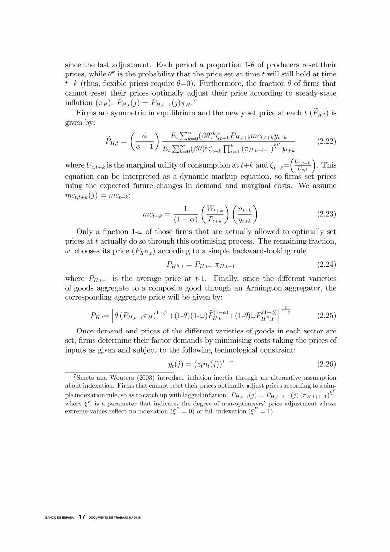
since the last adjustment. Each period a proportion 1-θ of producers reset theirprices, while θk is the probability that the price set at time t will still hold at timet+k (thus, flexible prices require θ=0). Furthermore, the fraction θ of firms thatcannot reset their prices optimally adjust their price according to steady-stateinflation (πH): PH,t(j) = PH,t−1(j)πH .7

Firms are symmetric in equilibrium and the newly set price at each t ( ePH,t) isgiven by:

ePH,t =

µφ

φ− 1

¶Et

P∞k=0(βθ)

kζt+kPH,t+kmct,t+kyt+k

Et

P∞k=0(βθ)

kζt+kQk

i=1 (πH,t+i−1)ξP yt+k

(2.22)

where Uc,t+k is the marginal utility of consumption at t+k and ζt+k=³Uc,t+kUc,t

´. This

equation can be interpreted as a dynamic markup equation, so firms set pricesusing the expected future changes in demand and marginal costs. We assumemct,t+k(j) = mct+k:

mct+k =1

(1− α)

µWt+k

Pt+k

¶µnt+kyt+k

¶(2.23)

Only a fraction 1-ω of those firms that are actually allowed to optimally setprices at t actually do so through this optimising process. The remaining fraction,ω, chooses its price (PHB ,t) according to a simple backward-looking rule

PHB ,t = PH,t−1πH,t−1 (2.24)

where PH,t−1 is the average price at t-1. Finally, since the different varietiesof goods aggregate to a composite good through an Armington aggregator, thecorresponding aggregate price will be given by:

PH,t=hθ (PH,t−1πH)

1−φ+(1-θ)(1-ω) eP (1−φ)H,t +(1-θ)ωP (1−φ)

HB ,t

i 11−φ

(2.25)

Once demand and prices of the different varieties of goods in each sector areset, firms determine their factor demands by minimising costs taking the prices ofinputs as given and subject to the following technological constraint:

yt(j) = (ztnt(j))1−α (2.26)

7Smets and Wouters (2003) introduce inflation inertia through an alternative assumptionabout indexation. Firms that cannot reset their prices optimally adjust prices according to a sim-ple indexation rule, so as to catch up with lagged inflation: PH,t+i(j) = PH,t+i−1(j) (πH,t+i−1)

ξP

where ξP is a parameter that indicates the degree of non-optimisers’ price adjustment whoseextreme values reflect no indexation (ξP = 0) or full indexation (ξP = 1).

10

BANCO DE ESPAÑA 17 DOCUMENTO DE TRABAJO N.º 0718

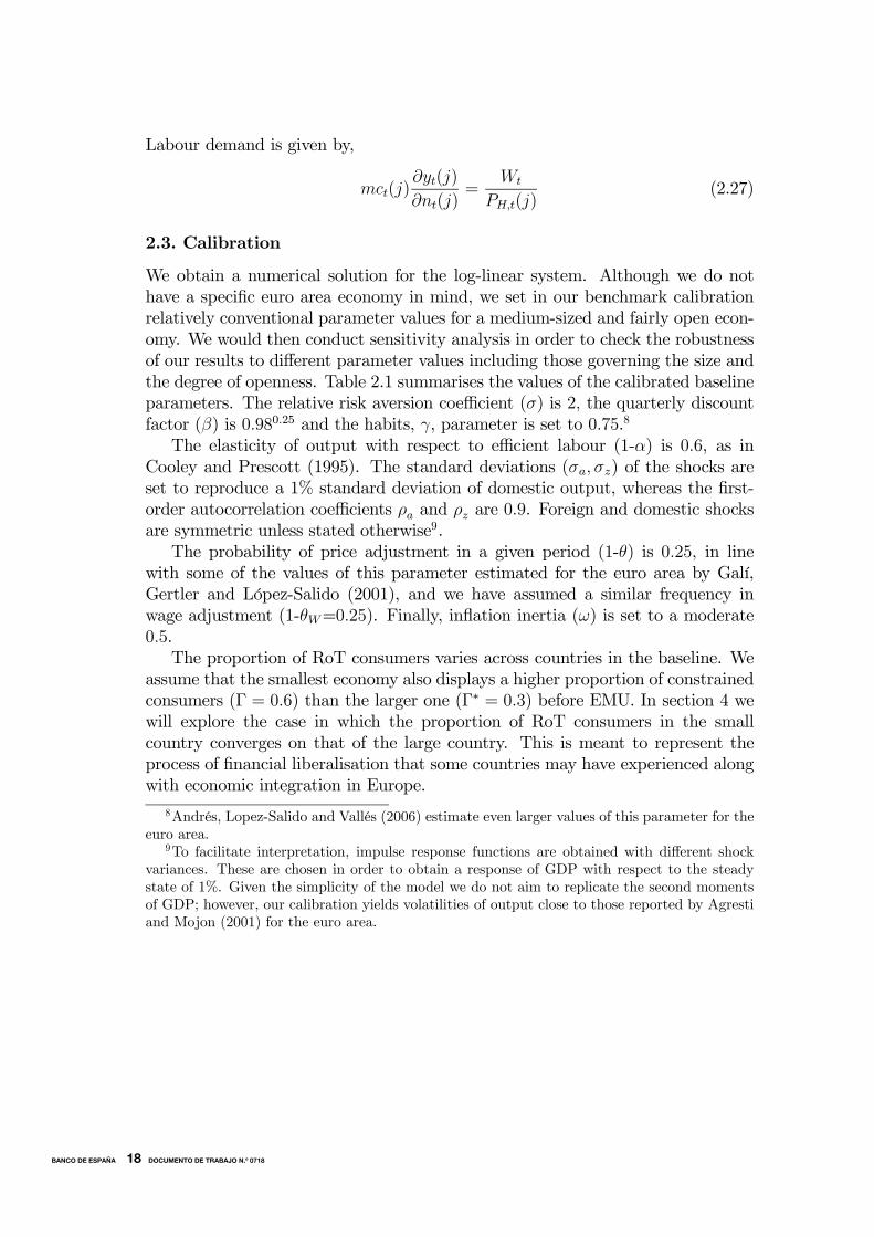
Labour demand is given by,

mct(j)∂yt(j)

∂nt(j)=

Wt

PH,t(j)(2.27)

2.3. Calibration

We obtain a numerical solution for the log-linear system. Although we do nothave a specific euro area economy in mind, we set in our benchmark calibrationrelatively conventional parameter values for a medium-sized and fairly open econ-omy. We would then conduct sensitivity analysis in order to check the robustnessof our results to different parameter values including those governing the size andthe degree of openness. Table 2.1 summarises the values of the calibrated baselineparameters. The relative risk aversion coefficient (σ) is 2, the quarterly discountfactor (β) is 0.980.25 and the habits, γ, parameter is set to 0.75.8

The elasticity of output with respect to efficient labour (1-α) is 0.6, as inCooley and Prescott (1995). The standard deviations (σa, σz) of the shocks areset to reproduce a 1% standard deviation of domestic output, whereas the first-order autocorrelation coefficients ρa and ρz are 0.9. Foreign and domestic shocksare symmetric unless stated otherwise9.The probability of price adjustment in a given period (1-θ) is 0.25, in line

with some of the values of this parameter estimated for the euro area by Galí,Gertler and López-Salido (2001), and we have assumed a similar frequency inwage adjustment (1-θW=0.25). Finally, inflation inertia (ω) is set to a moderate0.5.The proportion of RoT consumers varies across countries in the baseline. We

assume that the smallest economy also displays a higher proportion of constrainedconsumers (Γ = 0.6) than the larger one (Γ∗ = 0.3) before EMU. In section 4 wewill explore the case in which the proportion of RoT consumers in the smallcountry converges on that of the large country. This is meant to represent theprocess of financial liberalisation that some countries may have experienced alongwith economic integration in Europe.

8Andrés, Lopez-Salido and Vallés (2006) estimate even larger values of this parameter for theeuro area.

9To facilitate interpretation, impulse response functions are obtained with different shockvariances. These are chosen in order to obtain a response of GDP with respect to the steadystate of 1%. Given the simplicity of the model we do not aim to replicate the second momentsof GDP; however, our calibration yields volatilities of output close to those reported by Agrestiand Mojon (2001) for the euro area.

11

BANCO DE ESPAÑA 18 DOCUMENTO DE TRABAJO N.º 0718

We assume trade balance in the steady state. The share of imports of the do-mestic economy is 0.4, while the larger economy is much less open (0.4

¡CC∗

¢where¡

CC∗

¢=0.1 is the relative size). The elasticity of substitution between domestic and

imported consumption goods (ρ) is 1.5 (see Chari, Kehoe and McGrattan, 2002).The weights in aggregators (ωH , ω∗H , ωF and ω∗F ) that define the home bias areconsistent in the steady state with the calibrated values of ρ, C

C∗ ,CHC, C∗H

C, CFC∗ and

C∗FC∗ discussed above.The last set of parameters refers to the interest rate rule. In the baseline

model, we set the autocorrelation coefficient of the interest rate (ρr) equal to0.5 and the response to inflation deviations from target (ρπ) equal to 1.5. Thesevalues are consistent with the original Taylor rule, although they imply a slightlyquicker and more aggressive response of the interest rate to inflation than thatusually estimated for EMU countries. The steady-state level of gross inflation (π)is set at 1.020.25, i.e. the target level of the ECB. Finally, in the pre-MU years thedomestic interest rate is allowed to react to deviations of the exchange rate fromtarget (the foreign policy rate does not accommodate exchange rate variations).This reaction does not imply fixed exchange rates in the benchmark case, buta gradual upward (downward) adjustment in the nominal rate to prevent largedepreciations (appreciations): ρs=0.5.

2.4. The effects of a currency union on impulse-responses

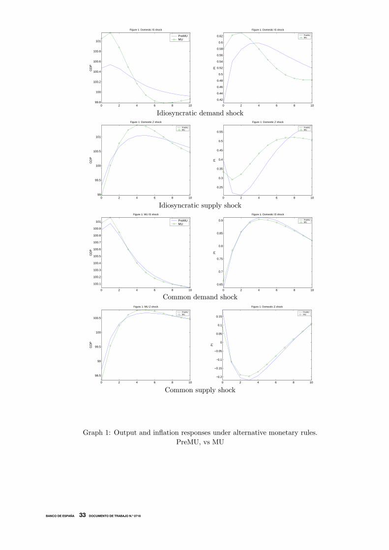
We now take a first look at the change in macroeconomic dynamics that oc-curs when both countries form a monetary union, comparing impulse-responsefunctions of output and inflation following different types of shocks under bothregimes. In all cases we take as a benchmark for comparison the model with aTaylor-type policy rule that includes a partial exchange rate peg,and an inertialcomponent with calibrated parameters as in Table 1. The foreign central bankhas in all cases the same Taylor reaction function (except that there is no pegto the exchange rate (ρ∗s = 0)). The shocks considered are: i) an idiosyncraticdemand shock, implemented as a shock to the domestic rate of time preference,at; ii) a common demand shock affecting at and a∗t ; iii) an idiosyncratic technologyshock implemented as a shock to domestic total factor productivity zt; and iv) acommon technology shock that entails changes in zt and z∗t .In the monetary union regime, the common interest rate is set according to a

Taylor rule based on area-wide variables weighted according to conventional para-meters (ρy=0.5, ρπ=1.5, ρR=0.5). Graph 2.1 presents impulse-response functions

12

BANCO DE ESPAÑA 19 DOCUMENTO DE TRABAJO N.º 0718

corresponding to the four shocks considered under the benchmark (pre-MU) andthe alternative (MU) regimes.After a domestic demand shock, the absence of compensating exchange rate

appreciation makes inflation increase initially by more under MU than under apartial peg. This higher inflation rate also induces a greater downward responseof the real rate (despite the reaction of the nominal rate) and leads to a strongeroutput response. Thus the moderate reaction of CPI inflation under a partial pegis the consequence of less demand pressure, lower GDP inflation, and the appre-ciation of the currency. This pattern is reversed after some quarters; the strongerresponse of domestic inflation under MU exacerbates the loss of competitivenessand makes output decrease more sharply than under the pre-MU regime.As for idiosyncratic technology shocks, inflation initially falls on impact in

both regimes, although the effect is less pronounced in the pre-MU regime as anexchange rate depreciation mitigates disinflation. Price and wage stickiness andthe presence of a high proportion of RoT households also make output fall tem-porarily in both regimes. As wages and prices gradually adjust to the productivityshock, output resumes an expansionary path. Under the pre-MU regime, interestrate hikes moderate output growth which therefore becomes less pronounced thanin the partial-peg regime. Since the expected increase of output is lower thanunder MU, lower expected marginal costs generate, beyond the very short term,lower inflation in the pre-MU regime.Not surprisingly, common shocks -whether demand or technological- do gen-

erate similar output and inflation responses under a partial or a full-peg regime.Since, under common shocks, the exchange rate moves little and home and for-eign economies are fairly symmetric, monetary policy actions under both regimesbecome virtually identical.

3. The empirical relevance of the monetary regime shift

As we have seen in the previous section, output and inflation dynamics are affectedwhen the economy enters a monetary union. The issue we explore now is whetherthe structural change prompted by the regime shift significantly affects the validityof reduced-form models estimated with pre-MU data to make inference on the MUregime.

13

BANCO DE ESPAÑA 20 DOCUMENTO DE TRABAJO N.º 0718

3.1. The metric

Since the most common use of reduced-form models is to conduct macroeconomicforecasts, we analyse the extent to which these models -estimated with data be-longing to the pre-MU regime- fail to provide accurate forecasts when the economyis under the MU regime. In our setting we will consider that the regime shift doesmatter empirically only if reduced-form models that ignore that shift significantlyunderperform similar reduced-form models estimated using data belonging to thenew regime. Our metric makes our analysis different from that followed in previ-ous literature on the empirical relevance of the Lucas critique. Most papers haveusually relied on tests of stability of parameters in reduced VARmodels following achange in the policy regime. While in statistical terms both approaches can hardlyoffer substantially different results, our metric allows us to derive a more directand economically meaningful measurement of the performance of VAR modelsafter a monetary regime shift.We will proceed as follows. We will first generate sets of data, each equivalent

to 25 years of quarterly data of output, inflation, interest rates and the exchangerate, for both (pre-MU and MU) regimes using the two-country DSGE model asoutlined in section 2.10 We will then estimate VAR models for each set of dataand compare the out-of-sample relative forecasting accuracy in the new (monetaryunion) regime of the VARs estimated with old (pre-MU) and new (MU) data.In order to generate data we assume that the economy is subject to the four

types of shocks considered in Section 2: namely, an idiosyncratic demand shock, anidiosyncratic supply shock, a common demand shock and a common supply shock.All shocks are independently distributed and follow a univariate AR process. Inthe initial calibration we have assumed that the variance of the demand shocks isthree times larger than that of the supply shocks. This is inspired by the relativeability of both shocks to explain by themselves the variance of output. Moreover,the idiosyncratic shocks are assumed to have the same variance as the commonshocks11. We will in any case explore the sensitivity of the results to changes inthose assumptions.Relative forecasting accuracy will be measured by means of ratios of mean-

squared errors (RMSE) and by the Diebold-Mariano (1995) test of equal forecasts

10Actually, we generate 150 observations and discard the first 50 to minimise the dependen-dence from the initial conditions.11According to Giannone and Reichlin (2006), the relative contribution of common and

country-specific shocks to output variability varies markedly across euro-area countries . How-ever, the average contribution of each type of shock is roughly 50% (see Table 4 in that paper).

14

BANCO DE ESPAÑA 21 DOCUMENTO DE TRABAJO N.º 0718

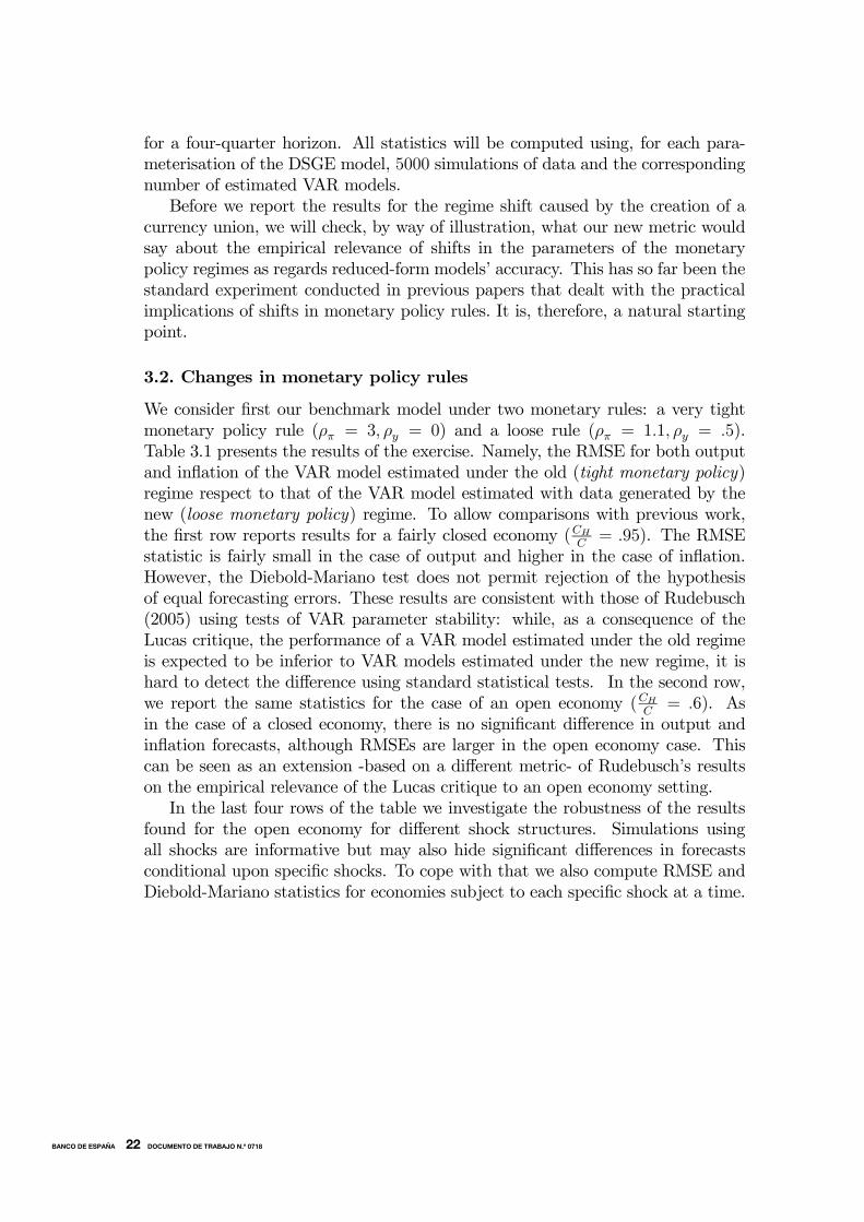
for a four-quarter horizon. All statistics will be computed using, for each para-meterisation of the DSGE model, 5000 simulations of data and the correspondingnumber of estimated VAR models.Before we report the results for the regime shift caused by the creation of a

currency union, we will check, by way of illustration, what our new metric wouldsay about the empirical relevance of shifts in the parameters of the monetarypolicy regimes as regards reduced-form models’ accuracy. This has so far been thestandard experiment conducted in previous papers that dealt with the practicalimplications of shifts in monetary policy rules. It is, therefore, a natural startingpoint.

3.2. Changes in monetary policy rules

We consider first our benchmark model under two monetary rules: a very tightmonetary policy rule (ρπ = 3, ρy = 0) and a loose rule (ρπ = 1.1, ρy = .5).Table 3.1 presents the results of the exercise. Namely, the RMSE for both outputand inflation of the VAR model estimated under the old (tight monetary policy)regime respect to that of the VAR model estimated with data generated by thenew (loose monetary policy) regime. To allow comparisons with previous work,the first row reports results for a fairly closed economy (CH

C= .95). The RMSE

statistic is fairly small in the case of output and higher in the case of inflation.However, the Diebold-Mariano test does not permit rejection of the hypothesisof equal forecasting errors. These results are consistent with those of Rudebusch(2005) using tests of VAR parameter stability: while, as a consequence of theLucas critique, the performance of a VAR model estimated under the old regimeis expected to be inferior to VAR models estimated under the new regime, it ishard to detect the difference using standard statistical tests. In the second row,we report the same statistics for the case of an open economy (CH

C= .6). As

in the case of a closed economy, there is no significant difference in output andinflation forecasts, although RMSEs are larger in the open economy case. Thiscan be seen as an extension -based on a different metric- of Rudebusch’s resultson the empirical relevance of the Lucas critique to an open economy setting.In the last four rows of the table we investigate the robustness of the results

found for the open economy for different shock structures. Simulations usingall shocks are informative but may also hide significant differences in forecastsconditional upon specific shocks. To cope with that we also compute RMSE andDiebold-Mariano statistics for economies subject to each specific shock at a time.

15

BANCO DE ESPAÑA 22 DOCUMENTO DE TRABAJO N.º 0718

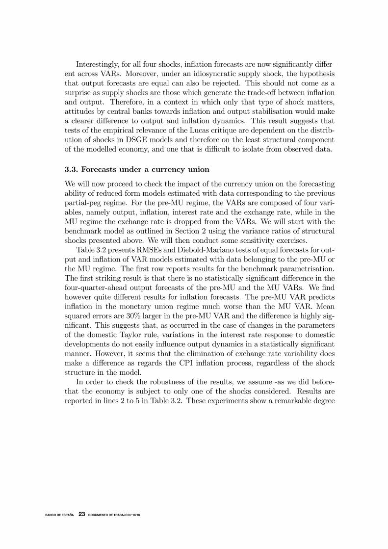
Interestingly, for all four shocks, inflation forecasts are now significantly differ-ent across VARs. Moreover, under an idiosyncratic supply shock, the hypothesisthat output forecasts are equal can also be rejected. This should not come as asurprise as supply shocks are those which generate the trade-off between inflationand output. Therefore, in a context in which only that type of shock matters,attitudes by central banks towards inflation and output stabilisation would makea clearer difference to output and inflation dynamics. This result suggests thattests of the empirical relevance of the Lucas critique are dependent on the distrib-ution of shocks in DSGE models and therefore on the least structural componentof the modelled economy, and one that is difficult to isolate from observed data.

3.3. Forecasts under a currency union

We will now proceed to check the impact of the currency union on the forecastingability of reduced-form models estimated with data corresponding to the previouspartial-peg regime. For the pre-MU regime, the VARs are composed of four vari-ables, namely output, inflation, interest rate and the exchange rate, while in theMU regime the exchange rate is dropped from the VARs. We will start with thebenchmark model as outlined in Section 2 using the variance ratios of structuralshocks presented above. We will then conduct some sensitivity exercises.Table 3.2 presents RMSEs and Diebold-Mariano tests of equal forecasts for out-

put and inflation of VAR models estimated with data belonging to the pre-MU orthe MU regime. The first row reports results for the benchmark parametrisation.The first striking result is that there is no statistically significant difference in thefour-quarter-ahead output forecasts of the pre-MU and the MU VARs. We findhowever quite different results for inflation forecasts. The pre-MU VAR predictsinflation in the monetary union regime much worse than the MU VAR. Meansquared errors are 30% larger in the pre-MU VAR and the difference is highly sig-nificant. This suggests that, as occurred in the case of changes in the parametersof the domestic Taylor rule, variations in the interest rate response to domesticdevelopments do not easily influence output dynamics in a statistically significantmanner. However, it seems that the elimination of exchange rate variability doesmake a difference as regards the CPI inflation process, regardless of the shockstructure in the model.In order to check the robustness of the results, we assume -as we did before-

that the economy is subject to only one of the shocks considered. Results arereported in lines 2 to 5 in Table 3.2. These experiments show a remarkable degree

16

BANCO DE ESPAÑA 23 DOCUMENTO DE TRABAJO N.º 0718

of similarity with the benchmark case in which all structural shocks are active. Inall four cases, RMSEs of output are relatively small and forecast differences areinsignificant. Moreover, in three cases we can reject the hypothesis that inflationforecasts are equal. Only in the case of a common demand shock is the differencenot statistically significant, although the RMSE is still quite large (1.34).In rows 6 to 10 we perform additional sensitivity analysis. In particular, we

allow for a smaller elasticity of intertemporal substitution (from σ = 2 to σ = 4),in order to increase the sensitivity of consumption to the interest rates (row 6),increase the share of domestic goods (from 60% to 80%) in the consumptionbasket (row 7), and increase the relative size (from 10% to 50%) of the homeeconomy in relation to the MU total (row 8). We finally allow for full flexibility ofprices (row 9) and wages (row 10). As can be seen, within a reasonable range ofparameter values, the results for the benchmark exercise hold also for economieswhich show more aversion to intertemporal substitution of consumption, or arenoticeably larger or more closed. Not surprisingly, though, when we allow for flexibleprices and/or wages, the statistically significant difference in inflation forecastsdisappears. Differences in the monetary regime are only important insofar asmonetary policy matters, as is the case in an economy with non-negligible nominalrigidities.

4. The impact of financial development

The process of nominal convergence and integration into a monetary union hasentailed structural transformations which may have affected the functioning ofthe economy in a significant manner. Therefore, by concentrating exclusively onthe effects of changes in the monetary regime, the analysis in the previous sectionmay fall short of identifying how EMU has actually changed output and inflationdynamics.By way of illustration, we assess in this section the impact of a relaxation of

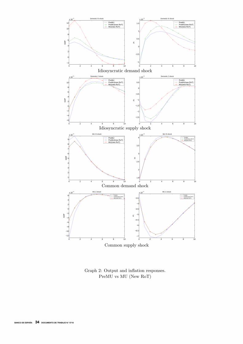
the financial constraints faced by the economy. In particular, we assume thatwhen the home country joins the currency union it also converges to the degreeof financial development enjoyed by the foreign country. In our simple model -without endogenous financial frictions- this can be approximated by lowering theproportion of consumers who do not have access to financial markets. Thus, theMU regime implies not only a common monetary policy but also an equal weightof constrained consumers in both economies (30%).As seen in Graph 4.1, the shape of responses to a demand shock is very similar

17

BANCO DE ESPAÑA 24 DOCUMENTO DE TRABAJO N.º 0718

to the case in which we ignore changes in the number of RoT consumers. However,differences in output and, to a lesser extent, inflation responses are larger. Asthere is now a higher proportion of agents that can borrow against future income,output can respond more to the persistent expansionary demand shock. This alsotranslates into higher inflation vis-à-vis the benchmark case.The effect of reducing the proportion of RoT consumers becomes more evident

when the economy faces an idiosyncratic technology shock. Output in the newMU regime grows persistently more (or falls less) than in the regime of partialpeg with a higher number of RoT consumers. Supply shocks tend to reduce hoursworked on impact in models with nominal price rigidities (Gali, 1999). This is sodespite the fact that current consumption of Ricardian consumers increases alongwith their permanent (future) income. On the contrary, RoT households mustreduce their consumption since their current labor income falls on impact. Thusthe impact output response is milder when the proportion of RoT consumers ishigh enough, and it can even be negative as in our model. Likewise, the responseof total consumption, and hence of output, is stronger when the proportion ofconsumers that trade in the financial market increases. The expansionary effecton output of the reduction in the proportion of constrained individuals more thanoffsets the expansionary impact of lower (nominal and real) interest rates in thecase of an independent monetary policy that partially accommodates movementsin the exchange rate. Besides, the MU regime avoids the appreciation of thecurrency that takes place in the benchmark case after two periods and henceinduces a stronger increase in the real wage and in consumption of the restrictedconsumers.The relaxation of financial constraints makes little difference on the impact

on output and inflation of a common demand shock. In the case of a commontechnology shock, output falls less in the new regime than in the benchmark caseas a higher number of unconstrained individuals permits the economy -througha permanent income effect- to moderate the short-term contractionary impact ofthe technology shock. Although the shock is common, easier access to credit inthe home economy prompts a significant country-specific expansionary effect.We now turn to check how the relative forecasting ability of pre-MU models

is affected when the MU regime also involves a relaxation of financial constraints.Table 4.1 presents the corresponding RMSEs and Diebold-Mariano tests. As canbe seen, in the new benchmark, the mean squared error of output in the pre-MUVARs is 21% larger than that of the corresponding MU VARs and the hypothesisof equal output forecasts can be rejected at conventional confidence levels. The

18

BANCO DE ESPAÑA 25 DOCUMENTO DE TRABAJO N.º 0718

RMSE for inflation is quite large (1.41) and highly significant. As expected, giventhe impulse response functions above, the main difference with respect to theresults in the previous section in which only the monetary rule changed is thatnow pre-MU VARs display a poorer output forecasting performance (rows 2 to5). This worse performance, relative to the case in which the proportion of RoTconsumers remains constant, is largely due to the impact of supply shocks.

5. Concluding remarks

The results discussed in the previous sections help assess the actual relevanceof the Lucas critique for models of countries that have recently joined the eurozone. Modellers are bound to experience considerable difficulties in representingthe dynamics followed by the main economic variables. Even considering similarattitudes by National Central Banks towards price and output stabilisation inthe pre-EMU period, the focus on euro-wide aggregates of the single monetarypolicy constitutes a substantial modification of the prevailing monetary regimethat may have non-trivial implications for output and price dynamics, particularlyif country-specific disturbances continue to be relevant.Still, we have seen that, from a practical point of view, the shift in the monetary

regime may not jeopardise much, by itself, the ability of standard reduced-formmodels to forecast output. This is broadly in line with previous research on therelevance of changes in the Fed policy rules for the stability of VAR models inthe US. In the MU case, however, our results suggest that problems are likely tobe much more severe when conducting inflation projections, as the eliminationof exchange variability between EMU countries does modify the inflation processin a statistically significant manner. Moreover, as EMU has been accompaniedby other structural transformations, the effects of the changes in the monetaryregime are likely to underestimate the relevant changes experienced in the dynam-ics followed by macroeconomic variables in the recent past. Our exercise drawson the fact that the reduction in interest rates together with greater competitionand integration in financial markets have increased the ability of individuals toobtain credit, and this has helped them to make more efficient intertemporal ex-penditure decisions. We have seen that these developments, alongside the shiftin the monetary regime, may significantly damage the accuracy of both inflationand output forecasts based on available VAR models.These results tend, in principle, to provide support for the effort, now under-

taken by many Eurosystem central banks, to develop DSGE models whose para-

19

BANCO DE ESPAÑA 26 DOCUMENTO DE TRABAJO N.º 0718

metrisation could be robust to changes in the monetary policy strategy. However,our findings also stress the complexity of the task. Failure by standard micro-founded models to properly address the relevant structural changes leads to aninaccurate and, as we have seen, sometimes misleading representation of the re-sponse of the economy to specific shocks.

References

[1] AGRESTI A., and B. MOJON (2001). Some Stylised Facts on the Euro AreaBusiness Cycle, European Central Bank, Working Paper No. 95.

[2] ANDRÉS, J., J. D. LÓPEZ-SALIDO and J. VALLÉS (2006). “Money in anEstimated Business Cycle Model of the Euro Area”. The Economic Journal,116 (April), pp. 457-477.

[3] BANK OF ENGLAND (2005). The Bank of England Quarterly Model.

[4] BENIGNO, P. (2001). Price Stability with Incomplete Risk Sharing, CEPR2854.

[5] CALVO, G. (1983). ”Staggered Prices in a Utility Maximizing Framework”,Journal of Monetary Economics, 12, pp. 383-398.

[6] CHARI, V., P. KEHOE and E. MCGRATTAN (2002). ”Can Sticky PriceModels Generate Volatile and Persistent Real Exchange Movements?”, Re-view of Economic Studies, vol. 69 (3), pp. 533-563.

[7] COOLEY, T. F., and E. C. PRESCOTT (1995). “Economic growth andbusiness cycles”, in Cooley, T. F., (ed.), Frontiers of Business Cycle Research,chapter 1, Princeton University Press, Princeton.

[8] DEL NEGRO, M., and F. SCHORFIDE (2003).“Take Your Model Bowl-ing: Forecasting with General Equilibrium Models”, Federal Reserve Bank ofAtlanta Economic Review, Fourth Quarter.

[9] – (2005). Monetary Policy Analysis with Potentially Misspecified Models,Federal Reserve Bank of Atlanta, Working Paper 2005-26.

[10] DEL NEGRO, M., F. SCHORFIDE, F. SMETS and R. WOUTERS (2004).On the Fit and Forecasting Performance of New Keynesian Models, Manu-script.

BANCO DE ESPAÑA 27 DOCUMENTO DE TRABAJO N.º 0718

[11] DIEBOLD, F. (1998). “The Past, Present and Future of Macroeconomic Fore-casting”, Journal of Economic Perspectives, 12, pp. 175-192.

[12] DIEBOLD, F., and R. MARIANO (1995). “Comparing Predictive Accuracy”,Journal of Business and Economic Statistics, American Statistical Associa-tion, vol. 13 (3), pp. 253-263, July.

[13] ERCEG, C., D. HENDERSON, and A. LEVIN (2000). “Optimal MonetaryPolicy with Staggered Wage and Price Contracts”, Journal of Monetary Eco-nomics, 46, pp. 281-313.

[14] ESTRELLA, A., and J. C. FUHRER (1998). Are Deep Parameters Stable?The Lucas Critique as an Empirical hypothesis, Manuscript.

[15] GALÍ, J. (1999). “Technology, Employment, and the Business Cycle: DoTechnology Shocks Explain Aggregate Fluctuations”. American EconomicReview, 89 (1), pp. 249-271.

[16] GALÍ, J., M. GERTLER and D. LÓPEZ-SALIDO (2001). “European Infla-tion Dynamics”, European Economic Review, 45, pp. 1237-1270.

[17] GALÍ, J., J. D. LÓPEZ-SALIDO and J. VALLÉS (2004). Understanding theEffects of Government Spending on Consumption, European Central Bank,Working Paper No. 339, April.

[18] GIANNONE, D., and L. REICHLIN (2006). Trends and cycles in the euroarea: how much heterogeneity and should we worry about it, European Cen-tral Bank, Working Paper No. 595.

[19] LINDÉ, J. (2001). “Testing for the Lucas Critique: A Quantitative Investi-gation”, American Economic Review, 91, pp. 986-1005.

[20] LUBIK, T., and P. SURICO (2006). The Lucas critique and the Stability ofEstimated Models, Federal Reserve Bank of Richmond, Working Paper No.06-05.

[21] LUCAS, R. E. (1976). “Econometric Policy Evaluation: a Critique”, in K.Brunner and A. Meltzer (eds.), The Phillips Curve and the Labor Market(Carnegie-Rochester Conference Series, vol. 1), Amsterdam, North-Holland.

BANCO DE ESPAÑA 28 DOCUMENTO DE TRABAJO N.º 0718

[22] LUCAS, R. E., and E. C. PRESCOT (1971). “Investment under Uncer-tainty”, Econometrica, 39, pp. 659-681.

[23] MALO DE MOLINA, J. L., and F. RESTOY (2005). “Recent trends incorporate and household finances in Spain: Macroeconomic implications”,Moneda y Crédito, 221, pp. 9-36.

[24] RUDEBUSCH, G. D. (2005). “Assessing the Lucas Critique in MonetaryPolicy Models”, Journal of Money Credit and Banking, 37 (2), pp. 245-272.

[25] SCHMITT-GROHÉ, S., and M. URIBE (2003). “Closing Small Open Econ-omy Models,” Journal of International Economics, 61, October, pp. 163-185.

[26] SMETS, F., and R. WOUTERS (2003). “An Estimated Dynamic Stochas-tic General Equilibrium Model of the Euro Area", Journal of the EuropeanEconomic Association, MIT Press, vol. 1 (5), pp. 1123-1175, September.

[27] TAYLOR, J. B. (1989). “Monetary Policy and Stability of MacroeconomicRelationships”, Journal of Applied Econometrics, 4, pp. 161-178.

[28] TAYLOR, J. B. (1999). “An Historical Analysis of Monetary Policy Rules”,in Monetary Policy Rules, edited by John B. Taylor, Chicago, Chicago Uni-versity Press, pp. 319-341.

[29] WOODFORD, M. (2003). Interest and Prices: Foundations of a Theory ofMonetary Policy, Princeton University Press.

BANCO DE ESPAÑA 29 DOCUMENTO DE TRABAJO N.º 0718

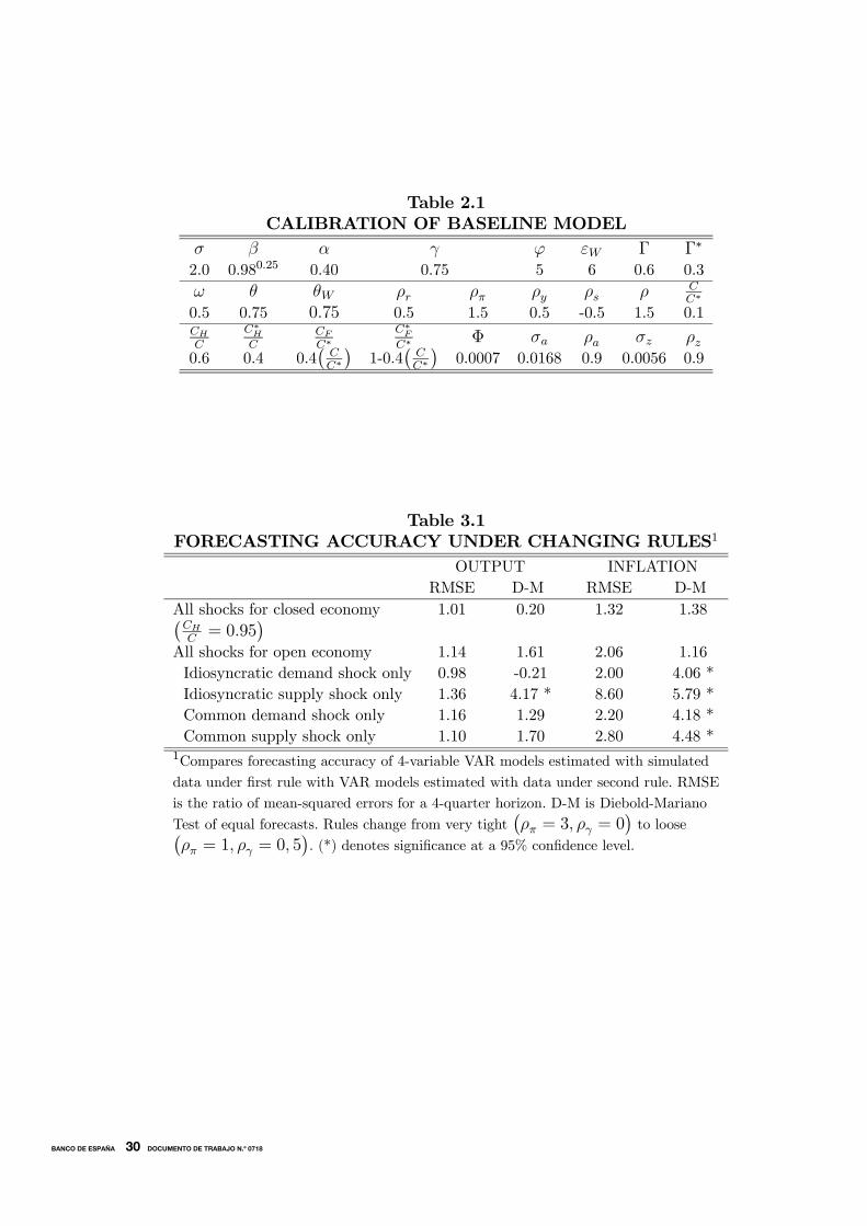
Table 2.1CALIBRATION OF BASELINE MODEL

σ β α γ ϕ εW Γ Γ∗

2.0 0.980.25 0.40 0.75 5 6 0.6 0.3ω θ θW ρr ρπ ρy ρs ρ C

C∗

0.5 0.75 0.75 0.5 1.5 0.5 -0.5 1.5 0.1CHC

C∗HC

CFC∗

C∗FC∗ Φ σa ρa σz ρz

0.6 0.4 0.4¡CC∗

¢1-0.4

¡CC∗

¢0.0007 0.0168 0.9 0.0056 0.9

Table 3.1FORECASTING ACCURACY UNDER CHANGING RULES1

OUTPUT INFLATIONRMSE D-M RMSE D-M

All shocks for closed economy 1.01 0.20 1.32 1.38¡CHC= 0.95

¢All shocks for open economy 1.14 1.61 2.06 1.16Idiosyncratic demand shock only 0.98 -0.21 2.00 4.06 *Idiosyncratic supply shock only 1.36 4.17 * 8.60 5.79 *Common demand shock only 1.16 1.29 2.20 4.18 *Common supply shock only 1.10 1.70 2.80 4.48 *

1Compares forecasting accuracy of 4-variable VAR models estimated with simulated

data under first rule with VAR models estimated with data under second rule. RMSE

is the ratio of mean-squared errors for a 4-quarter horizon. D-M is Diebold-Mariano

Test of equal forecasts. Rules change from very tight¡ρπ = 3, ργ = 0

¢to loose¡

ρπ = 1, ργ = 0, 5¢. (*) denotes significance at a 95% confidence level.

23

BANCO DE ESPAÑA 30 DOCUMENTO DE TRABAJO N.º 0718

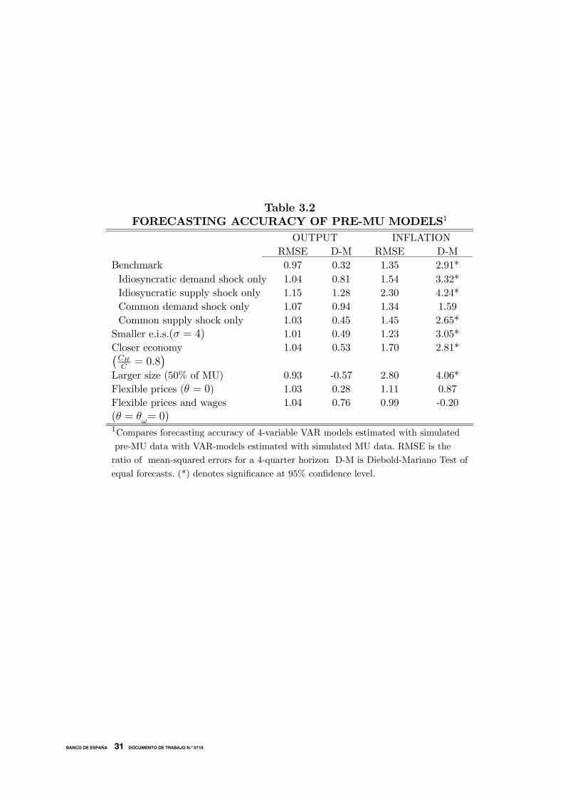
Table 3.2FORECASTING ACCURACY OF PRE-MU MODELS1

OUTPUT INFLATIONRMSE D-M RMSE D-M

Benchmark 0.97 0.32 1.35 2.91*Idiosyncratic demand shock only 1.04 0.81 1.54 3.32*Idiosyncratic supply shock only 1.15 1.28 2.30 4.24*Common demand shock only 1.07 0.94 1.34 1.59Common supply shock only 1.03 0.45 1.45 2.65*Smaller e.i.s.(σ = 4) 1.01 0.49 1.23 3.05*Closer economy 1.04 0.53 1.70 2.81*¡CHC= 0.8

¢Larger size (50% of MU) 0.93 -0.57 2.80 4.06*Flexible prices (θ = 0) 1.03 0.28 1.11 0.87Flexible prices and wages 1.04 0.76 0.99 -0.20(θ = θω= 0)1Compares forecasting accuracy of 4-variable VAR models estimated with simulated

pre-MU data with VAR-models estimated with simulated MU data. RMSE is the

ratio of mean-squared errors for a 4-quarter horizon D-M is Diebold-Mariano Test of

equal forecasts. (*) denotes significance at 95% confidence level.

24

BANCO DE ESPAÑA 31 DOCUMENTO DE TRABAJO N.º 0718

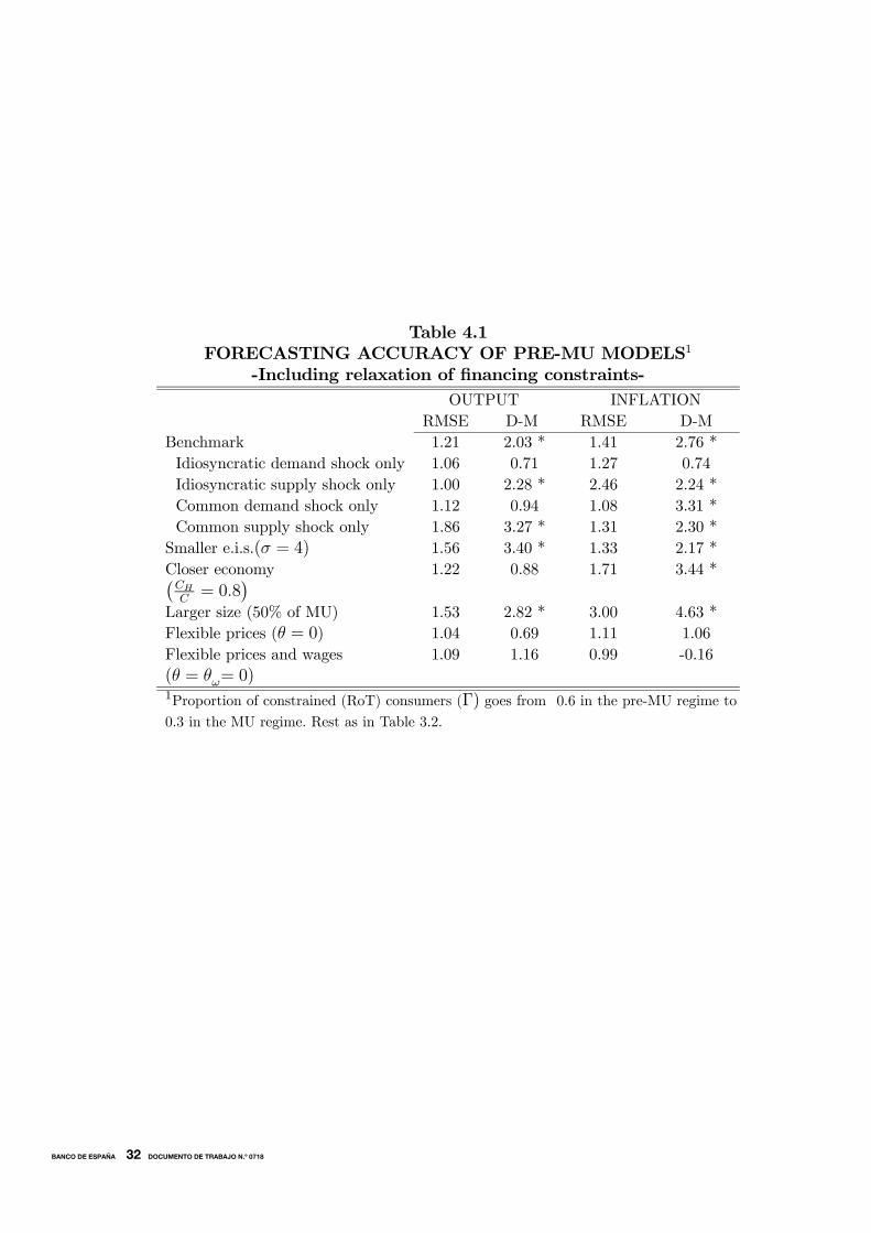
Table 4.1FORECASTING ACCURACY OF PRE-MU MODELS1

-Including relaxation of financing constraints-OUTPUT INFLATION

RMSE D-M RMSE D-MBenchmark 1.21 2.03 * 1.41 2.76 *Idiosyncratic demand shock only 1.06 0.71 1.27 0.74Idiosyncratic supply shock only 1.00 2.28 * 2.46 2.24 *Common demand shock only 1.12 0.94 1.08 3.31 *Common supply shock only 1.86 3.27 * 1.31 2.30 *Smaller e.i.s.(σ = 4) 1.56 3.40 * 1.33 2.17 *Closer economy 1.22 0.88 1.71 3.44 *¡CHC= 0.8

¢Larger size (50% of MU) 1.53 2.82 * 3.00 4.63 *Flexible prices (θ = 0) 1.04 0.69 1.11 1.06Flexible prices and wages 1.09 1.16 0.99 -0.16(θ = θω= 0)1Proportion of constrained (RoT) consumers (Γ) goes from 0.6 in the pre-MU regime to

0.3 in the MU regime. Rest as in Table 3.2.

25

BANCO DE ESPAÑA 32 DOCUMENTO DE TRABAJO N.º 0718

Idiosyncratic demand shock0 2 4 6 8 10

99.8

100

100.2

100.4

100.6

100.8

101

Figure 1: Domestic IS shock

GD

P

PreMUMU

0 2 4 6 8 10

0.42

0.44

0.46

0.48

0.5

0.52

0.54

0.56

0.58

0.6

0.62

Figure 1: Domestic IS shock

PI

PreMUMU

Idiosyncratic supply shock0 2 4 6 8 10

99

99.5

100

100.5

101

Figure 1: Domestic Z shock

GD

P

PreMUMU

0 2 4 6 8 10

0.25

0.3

0.35

0.4

0.45

0.5

0.55

Figure 1: Domestic Z shock

PI

PreMUMU

Common demand shock0 2 4 6 8 10

100.1

100.2

100.3

100.4

100.5

100.6

100.7

100.8

100.9

101

Figure 1: MU IS shock

GD

P

PreMUMU

0 2 4 6 8 10

0.65

0.7

0.75

0.8

0.85

0.9

Figure 1: Domestic IS shockP

I

PreMUMU

Common supply shock0 2 4 6 8 10

98.5

99

99.5

100

100.5

Figure 1: MU Z shock

GD

P

PreMUMU

0 2 4 6 8 10

−0.2

−0.15

−0.1

−0.05

0

0.05

0.1

0.15

Figure 1: Domestic Z shock

PI

PreMUMU

Graph 1: Output and inflation responses under alternative monetary rules.PreMU, vs MU

26

BANCO DE ESPAÑA 33 DOCUMENTO DE TRABAJO N.º 0718

Idiosyncratic demand shock0 2 4 6 8 10

−2

0

2

4

6

8

10

12

x 10−3 Domestic IS shock

GD

P

PreMUPreMU(new RoT)MU(new RoT)

0 2 4 6 8 10

−1

−0.5

0

0.5

1

1.5

x 10−3 Domestic IS shock

PI

PreMUPreMU(new RoT)MU(new RoT)

Idiosyncratic supply shock0 2 4 6 8 10

−6

−4

−2

0

2

4

6

8

10

x 10−3 Domestic Z shock

GD

P

PreMUPreMU(new RoT)MU(new RoT)

0 2 4 6 8 10

−2.5

−2

−1.5

−1

−0.5

0

0.5

x 10−3 Domestic Z shock

PI

PreMUPreMU(new RoT)MU(new RoT)

Common demand shock0 2 4 6 8 10

1

2

3

4

5

6

7

8

9

x 10−3 MU IS shock

GD

P

PreMUPreMU(new RoT)MU(new RoT)

0 2 4 6 8 10

1.5

2

2.5

3

3.5

4x 10

−3 MU IS shockP

IPreMUPreMU(new RoT)MU(new RoT)

Common supply shock

0 2 4 6 8 10

−12

−10

−8

−6

−4

−2

0

2

4

6

x 10−3 MU Z shock

GD

P

PreMUPreMU(new RoT)MU(new RoT)

0 2 4 6 8 10

−7

−6.5

−6

−5.5

−5

−4.5

−4

−3.5

x 10−3 MU Z shock

PI

PreMUPreMU(new RoT)MU(new RoT)

Graph 2: Output and inflation responses.PreMU vs MU (New RoT)

27

BANCO DE ESPAÑA 34 DOCUMENTO DE TRABAJO N.º 0718

BANCO DE ESPAÑA PUBLICATIONS

WORKING PAPERS1

0601 ARTURO GALINDO, ALEJANDRO IZQUIERDO AND JOSÉ MANUEL MONTERO: Real exchange rates,

dollarization and industrial employment in Latin America.

0602 JUAN A. ROJAS AND CARLOS URRUTIA: Social security reform with uninsurable income risk and endogenous

borrowing constraints.

0603 CRISTINA BARCELÓ: Housing tenure and labour mobility: a comparison across European countries.

0604 FRANCISCO DE CASTRO AND PABLO HERNÁNDEZ DE COS: The economic effects of exogenous fiscal

shocks in Spain: a SVAR approach.

0605 RICARDO GIMENO AND CARMEN MARTÍNEZ-CARRASCAL: The interaction between house prices and loans

for house purchase. The Spanish case.

0606 JAVIER DELGADO, VICENTE SALAS AND JESÚS SAURINA: The joint size and ownership specialization in

banks’ lending.

0607 ÓSCAR J. ARCE: Speculative hyperinflations: When can we rule them out?

0608 PALOMA LÓPEZ-GARCÍA AND SERGIO PUENTE: Business demography in Spain: determinants of firm survival.

0609 JUAN AYUSO AND FERNANDO RESTOY: House prices and rents in Spain: Does the discount factor matter?

0610 ÓSCAR J. ARCE AND J. DAVID LÓPEZ-SALIDO: House prices, rents, and interest rates under collateral

constraints.

0611 ENRIQUE ALBEROLA AND JOSÉ MANUEL MONTERO: Debt sustainability and procyclical fiscal policies in Latin

America.

0612 GABRIEL JIMÉNEZ, VICENTE SALAS AND JESÚS SAURINA: Credit market competition, collateral

and firms’ finance.

0613 ÁNGEL GAVILÁN: Wage inequality, segregation by skill and the price of capital in an assignment model.

0614 DANIEL PÉREZ, VICENTE SALAS AND JESÚS SAURINA: Earnings and capital management in alternative loan

loss provision regulatory regimes.

0615 MARIO IZQUIERDO AND AITOR LACUESTA: Wage inequality in Spain: Recent developments.

0616 K. C. FUNG, ALICIA GARCÍA-HERRERO, HITOMI IIZAKA AND ALAN SUI: Hard or soft? Institutional reforms and

infraestructure spending as determinants of foreign direct investment in China.

0617 JAVIER DÍAZ-CASSOU, ALICIA GARCÍA-HERRERO AND LUIS MOLINA: What kind of capital flows does the IMF

catalyze and when?

0618 SERGIO PUENTE: Dynamic stability in repeated games.

0619 FEDERICO RAVENNA: Vector autoregressions and reduced form representations of DSGE models.

0620 AITOR LACUESTA: Emigration and human capital: Who leaves, who comes back and what difference does it make?

0621 ENRIQUE ALBEROLA AND RODRIGO CÉSAR SALVADO: Banks, remittances and financial deepening in

receiving countries. A model.

0622 SONIA RUANO-PARDO AND VICENTE SALAS-FUMÁS: Morosidad de la deuda empresarial bancaria

en España, 1992-2003. Modelos de la probabilidad de entrar en mora, del volumen de deuda en mora y del total

de deuda bancaria, a partir de datos individuales de empresa.

0623 JUAN AYUSO AND JORGE MARTÍNEZ: Assessing banking competition: an application to the Spanish market

for (quality-changing) deposits.

0624 IGNACIO HERNANDO AND MARÍA J. NIETO: Is the Internet delivery channel changing banks’ performance? The

case of Spanish banks.

0625 JUAN F. JIMENO, ESTHER MORAL AND LORENA SAIZ: Structural breaks in labor productivity growth: The

United States vs. the European Union.

0626 CRISTINA BARCELÓ: A Q-model of labour demand.

0627 JOSEP M. VILARRUBIA: Neighborhood effects in economic growth.

0628 NUNO MARTINS AND ERNESTO VILLANUEVA: Does limited access to mortgage debt explain why young adults

live with their parents?

0629 LUIS J. ÁLVAREZ AND IGNACIO HERNANDO: Competition and price adjustment in the euro area.

0630 FRANCISCO ALONSO, ROBERTO BLANCO AND GONZALO RUBIO: Option-implied preferences adjustments,

density forecasts, and the equity risk premium.

1. Previously published Working Papers are listed in the Banco de España publications catalogue.

0631 JAVIER ANDRÉS, PABLO BURRIEL AND ÁNGEL ESTRADA: BEMOD: A dsge model for the Spanish economy

and the rest of the Euro area.

0632 JAMES COSTAIN AND MARCEL JANSEN: Employment fluctuations with downward wage rigidity: The role of

moral hazard.

0633 RUBÉN SEGURA-CAYUELA: Inefficient policies, inefficient institutions and trade.

0634 RICARDO GIMENO AND JUAN M. NAVE: Genetic algorithm estimation of interest rate term structure.

0635 JOSÉ MANUEL CAMPA, JOSÉ M. GONZÁLEZ-MÍNGUEZ AND MARÍA SEBASTIÁ-BARRIEL: Non-linear

adjustment of import prices in the European Union.

0636 AITOR ERCE-DOMÍNGUEZ: Using standstills to manage sovereign debt crises.

0637 ANTON NAKOV: Optimal and simple monetary policy rules with zero floor on the nominal interest rate.

0638 JOSÉ MANUEL CAMPA AND ÁNGEL GAVILÁN: Current accounts in the euro area: An intertemporal approach.

0639 FRANCISCO ALONSO, SANTIAGO FORTE AND JOSÉ MANUEL MARQUÉS: Implied default barrier in credit

default swap premia. (The Spanish original of this publication has the same number.)

0701 PRAVEEN KUJAL AND JUAN RUIZ: Cost effectiveness of R&D and strategic trade policy.

0702 MARÍA J. NIETO AND LARRY D. WALL: Preconditions for a successful implementation of supervisors’ prompt

corrective action: Is there a case for a banking standard in the EU?

0703 PHILIP VERMEULEN, DANIEL DIAS, MAARTEN DOSSCHE, ERWAN GAUTIER, IGNACIO HERNANDO,

ROBERTO SABBATINI AND HARALD STAHL: Price setting in the euro area: Some stylised facts from individual

producer price data.

0704 ROBERTO BLANCO AND FERNANDO RESTOY: Have real interest rates really fallen that much in Spain?

0705 OLYMPIA BOVER AND JUAN F. JIMENO: House prices and employment reallocation: International evidence.

0706 ENRIQUE ALBEROLA AND JOSÉ M.ª SERENA: Global financial integration, monetary policy and reserve

accumulation. Assessing the limits in emerging economies.

0707 ÁNGEL LEÓN, JAVIER MENCÍA AND ENRIQUE SENTANA: Parametric properties of semi-nonparametric

distributions, with applications to option valuation.

0708 DANIEL NAVIA AND ENRIQUE ALBEROLA : Equilibrium exchange rates in the new EU members: external

imbalances vs. real convergence.

0709 GABRIEL JIMÉNEZ AND JAVIER MENCÍA: Modelling the distribution of credit losses with observable and latent

factors.

0710 JAVIER ANDRÉS, RAFAEL DOMÉNECH AND ANTONIO FATÁS: The stabilizing role of government size.

0711 ALFREDO MARTÍN-OLIVER, VICENTE SALAS-FUMÁS AND JESÚS SAURINA: Measurement of capital stock

and input services of Spanish banks.

0712 JESÚS SAURINA AND CARLOS TRUCHARTE: An assessment of Basel II procyclicality in mortgage portfolios.

0713 JOSÉ MANUEL CAMPA AND IGNACIO HERNANDO: The reaction by industry insiders to M&As in the European

financial industry.

0714 MARIO IZQUIERDO, JUAN F. JIMENO AND JUAN A. ROJAS: On the aggregate effects of immigration in Spain.

0715 FABIO CANOVA AND LUCA SALA: Back to square one: identification issues in DSGE models.

0716 FERNANDO NIETO: The determinants of household credit in Spain.

0717 EVA ORTEGA, FERNANDO BURRIEL, JOSÉ LUIS FERNÁNDEZ, EVA FERRAZ AND SAMUEL HURTADO:

Actualización del modelo trimestral del Banco de España.

0718 JAVIER ANDRÉS AND FERNANDO RESTOY: Macroeconomic modelling in EMU: How relevant is the change in

regime?

Unidad de PublicacionesAlcalá, 522; 28027 Madrid

Telephone +34 91 338 6363. Fax +34 91 338 6488e-mail: [email protected]

www.bde.es