Macroeconomic Consequences of Natural Disasters

Policy Research Working Paper 9943

Macroeconomic Consequences of Natural Disasters

A Modeling Proposal and Application to Floods and Earthquakes in Turkey

Stéphane Hallegatte Charl Jooste

Florent McIsaac

Macroeconomics, Trade and Investment Global Practice &Climate Change GroupFebruary 2022

Pub

lic D

iscl

osur

e A

utho

rized

Pub

lic D

iscl

osur

e A

utho

rized

Pub

lic D

iscl

osur

e A

utho

rized

Pub

lic D

iscl

osur

e A

utho

rized

Produced by the Research Support Team

Abstract

The Policy Research Working Paper Series disseminates the findings of work in progress to encourage the exchange of ideas about development issues. An objective of the series is to get the findings out quickly, even if the presentations are less than fully polished. The papers carry the names of the authors and should be cited accordingly. The findings, interpretations, and conclusions expressed in this paper are entirely those of the authors. They do not necessarily represent the views of the International Bank for Reconstruction and Development/World Bank and its affiliated organizations, or those of the Executive Directors of the World Bank or the governments they represent.

Policy Research Working Paper 9943

Turkey is vulnerable to natural disasters that can generate substantial damages to public and private sector infrastruc-ture capital. Earthquakes and floods are the most frequent hazards today, and flood risks are expected to increase with climate change. To ensure stability and growth and min-imize the welfare impact of these disasters, these shocks need to be managed and accounted for in macro-fiscal and monetary policy. To support this process, the World Bank Macrostructural Model is adapted to assess the macroeco-nomic effects of natural (geophysical or climate-related) disasters. The macroeconomic model is extended on several fronts: (1) a distinction is made between infrastructure and non-infrastructure capital, with complementary or substi-tutability between the two categories; (2) the production function is adjusted to account for short-term complemen-tarity across capital assets; (3) the reconstruction process is modeled in a way that accounts for post-disaster constraints,

with distinct processes for the reconstruction of public and private assets. The results show that destroyed infra-structure capital makes the remaining non-infrastructure capital less productive, which means that disasters reduce the total stock of capital, but also its productivity. The welfare impact of a disaster—proxied by the discounted consumption loss—is found to increase non-linearly with direct asset losses. Macroeconomic responses reduce the welfare impact of minor disasters but magnify it when direct asset losses exceed the economy’s absorption capacity. The welfare impact also depends on the pre-existing economic situation, the ability of the economy to reallocate resources toward reconstruction, and the response of the monetary policy. Appropriate macro-fiscal and monetary policies offer cost-effective opportunities to mitigate the welfare impact of major disasters.

This paper is a product of the Macroeconomics, Trade and Investment Global Practicea and the Climage Change Group. It is part of a larger effort by the World Bank to provide open access to its research and make a contribution to development policy discussions around the world. Policy Research Working Papers are also posted on the Web at http://www.worldbank.org/prwp. The authors may be contacted at at [email protected], [email protected], and [email protected].

Macroeconomic Consequences of Natural Disasters: A Modeling Proposal and Application to Floods and

Earthquakes in Turkey*

Stephane Hallegatte1, Charl Jooste2, and Florent McIsaac3

1,2,3World Bank

Keywords: macro-structural model; natural disasters; earthquakes; floods; climate.JEL Classification: C10; C50; E52; Q54.

*We thank Hans Anand Beck, Somik Lall, Miles Parker, and Christian Schoder for their helpful commentson an earlier version of this article. All remaining errors and opinions are our own.

1 Introduction

All countries are exposed to various and varying natural hazards, either geophysical likeearthquakes or climate-related such as floods, heatwaves, or windstorms. Increase in pop-ulation, economic growth, and urbanization are associated with a rapid increase in theeconomic damages caused by disasters. In the future, the increase in global average tem-perature induced by climate change is expected to increase the intensity and frequency ofextreme weather and climate events further (IPCC, 2012), possibly leading to larger losses.Beyond physical damages — in the form of destroyed houses, roads, or factories — disas-ters also affect the functioning of the economic systems, with complex effects transmittedthrough supply chains and macroeconomic feedback. This paper proposes a model to in-vestigate and quantify the transition channels of disasters through the capital structure in aconsistent macroeconomic framework. The model is applied to flood and earthquake risksin Turkey.

This paper describes a methodological approach, extending Burns et al. (2019); Burnsand Jooste (2019), to model physical capital stocks more granularly using Turkey as a casestudy. Macroeconomic models are used by finance ministries or central banks to quantifythe effects of shocks and provide alternative paths for the economy. However, macroeco-nomic models have not been designed to capture specific impacts of natural disasters, suchas the large share of damages affecting infrastructure and buildings (compared with othercapital assets), or the practical constraints slowing down a reconstruction process (Halle-gatte and Vogt-Schilb, 2019). The main objective of this paper is to capture the structureand dynamics of natural shocks to capital and their link to economic losses and economicdecision making. The modeling approach suggested in this paper could be applied to awide range of disasters, provided they are channeled through the same mechanisms asthose considered here for floods and earthquakes. It can also be used to explore howan increase in the frequency and intensity of hazards could translate into larger physicallosses, and eventually larger macroeconomic impacts (including GDP, consumption, publicdeficit, public debt, inflation, etc.). And it could help explore how various macroeconomicor monetary policies can reduce macroeconomic (and welfare) losses, even if physical dam-ages remain unchanged.

To incorporate disasters and mitigation strategies, the model architecture includes asegmentation of capital between infrastructure and non-infrastructure capital, and withinthis asset class, between the private and public sectors. The cost and return on capital arecalculated using a nested structure with a constant elasticity of substitution. This papercan be viewed as an extension of Burns et al. (2020) along three lines. First, capital isdivided into several dimensions and mapped to time series data. Second, the substitutabil-ity between infrastructure and non-infrastructure capital is estimated. This elasticity willtherefore amplify or attenuate the damage, depending on the degree of substitution. Third,the modeling of post-disaster reconstruction takes into account the difference between pri-vate and public reconstruction and the different damages they face.

Earthquakes and floods are the most frequent disasters in Turkey (see fig. 1). Andaccording to data reported in Ocal (2019), earthquakes are the most destructive: theyaccount for 92.6% of the number of damaged buildings and 95.9% of the number ofdemolished buildings in Turkey between 1900 and 2018. In this paper, we explore the

2

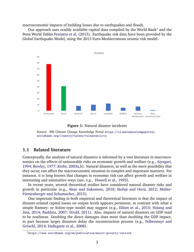
macroeconomic impacts of building losses due to earthquakes and floods.Our approach uses readily available capital data compiled by the World Bank1 and the

Penn World Tables Feenstra et al. (2015). Earthquake risk data have been provided by theGlobal Earthquake Model, using the 2013 Euro-Mediterranean seismic risk model.

0

10

20

30

40

50

60

70

80

90

Earthquake Flood Epidemic Storm Landslide Wildfire Extremetemperature

Massmovement (dry)

Incidents

Figure 1: Natural disaster incidents

Source: WB Climate Change Knowledge Portal https://climateknowledgeportal.worldbank.org/country/turkey/vulnerability.

1.1 Related literature

Conceptually, the analysis of natural disasters is informed by a vast literature in macroeco-nomics on the effects of uninsurable risks on economic growth and welfare (e.g., Aiyagari,1994; Bewley, 1977; Krebs, 2003a,b). Natural disasters, as well as the mere possibility thatthey occur, can affect the macroeconomic situation in complex and important manners. Forinstance, it is long known that changes in economic risk can affect growth and welfare ininteresting and unintuitive ways (see, e.g., Howell et al., 1993).

In recent years, several theoretical studies have considered natural disaster risks andgrowth in particular (e.g., Akao and Sakamoto, 2018; Ikefuji and Horii, 2012; Muller-Furstenberger and Schumacher, 2015).

One important finding in both empirical and theoretical literature is that the impact ofdisaster-related capital losses on output levels appears persistent, in contrast with what asimple Ramsey- or Solow-type model may suggest (e.g., Elliott et al., 2015; Hsiang andJina, 2014; Raddatz, 2007; Strobl, 2011). Also, impacts of natural disasters on GDP tendto be nonlinear. Doubling the direct damages does more than doubling the GDP impact,in part because larger disasters delay the reconstruction process (e.g., Felbermayr andGroschl, 2014; Hallegatte et al., 2008).

1https://www.worldbank.org/en/publication/macro-poverty-outlook

3

The literature also stresses the importance of considering differences in substitutionoptions over the short-term (compared with long-term substitutability). Physical damagesfrom disasters interact with the economy in a complex manner, through the network ofsupply chains (Baqaee and Farhi, 2020; Barrot and Sauvagnat, 2016; Boehm et al., 2019;Henriet et al., 2012; Inoue and Todo, 2019) and the role of infrastructure systems, fromtransport systems to electricity grids (Colon et al., 2021; Rose and Liao, 2005; Rose andWei, 2013). In particular, destroyed infrastructure capital can make the remaining non-infrastructure capital unproductive, magnifying output losses (Hallegatte and Vogt-Schilb,2019).

To capture some of these effects, Hallegatte et al. (2007) introduce a specific produc-tion function to reproduce the short-term impact of disasters, accounting for the shorttimescales that do not allow (1) the same substitution among production factors as overthe long-term, and (2) the reallocation of post-disaster assets to their most productiveuses. The model also includes constraints on the reconstruction-related investments tomake the model dynamics more consistent with observed disaster aftermath. With thosechanges, the model suggests that the GDP impact of disasters remain limited unless theirfrequency and intensity exceed the ability of the economy to reconstruct (in which casedisasters start to show a cumulative effects that can significantly reduce the GDP level).The model also finds that disaster impacts are context-dependent, particularly in respectto the pre-existing macroeconomic situation, with disasters occurring during recessionshaving smaller impacts on GDP, as the reconstruction process can mobilize idle resourceswithout crowding out other investments (Hallegatte and Ghil, 2008). Our work extendsthis work by representing the capital stock through different categories (infrastructure andnon-infrastructure, public and private) to better represent the effect of capital losses onoutputs, and real-world constraint on reconstruction investments.

Our work also builds on recent papers on the interaction of natural risk and macroe-conomic factors. Isore and Szczerbowicz (2017) show that standard real business cyclemodels produce puzzling results when modeling disasters. They produce an increase inconsumption when output and asset values fall in response to disaster risk. In this setup,the risk-free rate also falls in response to the disaster risk. To solve this puzzle, Isore andSzczerbowicz (2017) include sticky prices and an elasticity of substitution less than one.In their model, the discount rate varies over time and is a function of time-varying disas-ter risk (thus incorporating the role of preferences and uncertainty). This configurationgenerates an increase in patience and thus an increase in savings when the elasticity ofsubstitution is less than one. If the elasticity of substitution is greater than one, this willresult in an increase in impatience and an increase in consumption in response to a changein disaster risk. Another important feature of this model is the role of price flexibility. Ifconsumers save in the presence of disaster risk, then investment will increase and result inhigher output when prices are flexible. To counteract this result, sticky prices are requiredso that the demand for capital decreases with disaster risk and thus generates lower invest-ment. Finally, the risk premium will now increase in response to disaster risk, with an evenlarger response if agents are risk averse. Through careful calibration, this modification ofthe standard real business cycle model is able to produce a decline in output as well as adecline in consumption and investment with the change in the probability of an event.

Another dynamic stochastic general equilibrium (DSGE) modeling approach by Wrightand Borda (2016) represents disasters by adjusting the capital stock. It also includes the

4

country risk gap as a function of total factor productivity and the disaster shock. Thismodeling approach does not incorporate the fixed wage and discount rate characteristicsof Isore and Szczerbowicz (2017). In this configuration, consumption increases for manyof the countries while output and investment decrease, again producing the conundrumhighlighted above.

Camacho and Sun (2017) extend a Ramsey model to account for reconstruction timesafter a natural disaster, in this case earthquakes, and resilience capital to describe theeconomic impact in Japan and Italy. The numerical exercise shows that a large share ofprevention capital (e.g., in a country like Japan with high resilience standards) reducesearthquake damage significantly for large shocks. However, the losses can be considerablefor intense earthquakes. In the model, consumption absorbs most of the losses when re-silience capital is low. However, the share of consumption in GDP increases when adaptivecapital is low in earthquakes. This is consistent with the DSGE literature regarding theoptimal consumption smoothing scheme.

Marto et al. (2018) build a dynamic small open economy model with permanent dam-ages to both public and private capital. Disaster leads to temporary losses in productivity,inefficiencies during the rebuilding process, and damage to the sovereign’s creditworthi-ness. In the model, investment in resilient infrastructure can be useful, especially if it isconsidered complementary to standard infrastructure, because it increases the marginalproduct of private capital, attracting private investment, while helping to withstand theimpact of the natural disaster. The modeling framework in our paper shares many similarcharacteristics.

Bakkensen and Barrage (2021) reconciles empirical and structural methodologies tomodel the economic impact of natural disasters. Instead of running reduced-form regres-sions of natural disasters on output per person, they identify the direct impacts on thestructural determinants of growth (e.g., capital, labor, and total factor productivity). Theirmodeling approach has three important features: (i) separation of the effect of risk fromthe effect of a disaster; (ii) endogenous adaptation through changes in investment and sav-ings; and (iii) computing welfare costs associated with weather and climate risks. Whilethey find that welfare is reduced by climate shocks (in this case cyclones), the impact oneconomic growth is smaller, in part due to the impact of risk (even unrealized) on precau-tionary savings.

Finally, our analysis is part of a parallel literature on chronic physical risk, climatechange, and economic growth. There is a growing body of literature that contributes tothe active discussion on the evaluation of economic damage functions (e.g., Burke et al.,2015; Nordhaus and Moffat, 2017). With respect to incorporating climate disasters intomacroeconomic models, some pioneering analysis of Fankhauser and Tol (2005); Mooreand Diaz (2015) incorporate results from Dell et al. (2012) into the DICE model that hadits origin in Nordhaus (1992). Because the estimates of the impact on output growth do notprovide a clear match with the macroeconomic models, Moore and Diaz (2015) considercalibrating capital depreciation (and/or TFP growth) to match the reduced-form estimates.The choice between the two appears quantitatively significant in terms of optimal mitiga-tion dynamic. A similar question arises in Dietz and Stern (2015); Fankhauser and Tol(2005), which extend DICE to a long-run endogenous growth framework with capital- orinvestment-based knowledge spillovers. These papers show how the channeling of dam-ages, whether in consumption or investment, and the macro-modeling framework chosen,

5

are critical to assessing the impact of climate disasters.The modeling framework in this paper attempts to shed light on these channels by

reinforcing the empirical and theoretical arguments in disaster modeling, whether naturalor climate induced.

1.2 Natural disaster capital modeling considerations

First, we adapt the physical capital structure of the World Bank’s macrostructural modelMFMod (Burns et al., 2019) to capture the transmission channels of natural disasters inthe macroeconomic framework. We assume that the aggregate capital stock is a combi-nation of two types of capital, infrastructure and non-infrastructure, and distinguish thecontributions of private and public investments to the capital stock.

Second, we use granular earthquake and flood damage data, and translate aggregateimpacts into impacts to the various types of capital in the model. This allows to explorethe importance of the substitutability between different types of capital, as opposed toassuming full substitutability (like in models where the capital stock is represented onlyby an aggregate value). Differentiated impacts across capital types allows us to representthe fact that disasters reduce the stock of capital, but also lead to the mis-allocation of theremaining capital, thereby reducing overall productivity (as discussed in Hallegatte et al.(2007); Hallegatte and Vogt-Schilb (2019) and empirically observed by Bakkensen andBarrage (2021) and Dieppe et al. (2020)).

Finally, we take into account realistic reconstruction times, which in reality are con-straints faced by institutional, technological deficiencies, and a lack of financial access.The distinction between public and private capital also allows us to account for differentdecision-making processes, sources of financing, and constraints on timing for rebuildingthese different asset types.

The modeling of disasters require several data sets and methodological approaches.Figure 2 summarizes the key elements related to disasters, which include the identificationof hazards, vulnerabilities and exposures.

6

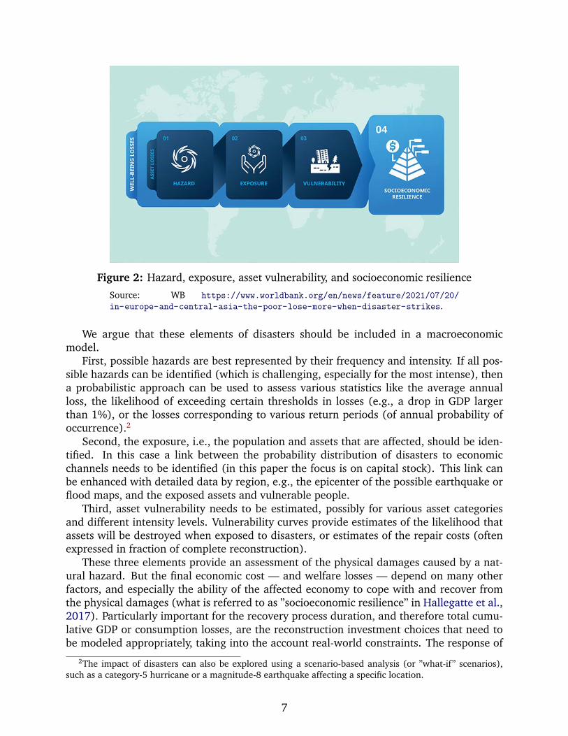
Figure 2: Hazard, exposure, asset vulnerability, and socioeconomic resilience

Source: WB https://www.worldbank.org/en/news/feature/2021/07/20/

in-europe-and-central-asia-the-poor-lose-more-when-disaster-strikes.

We argue that these elements of disasters should be included in a macroeconomicmodel.

First, possible hazards are best represented by their frequency and intensity. If all pos-sible hazards can be identified (which is challenging, especially for the most intense), thena probabilistic approach can be used to assess various statistics like the average annualloss, the likelihood of exceeding certain thresholds in losses (e.g., a drop in GDP largerthan 1%), or the losses corresponding to various return periods (of annual probability ofoccurrence).2

Second, the exposure, i.e., the population and assets that are affected, should be iden-tified. In this case a link between the probability distribution of disasters to economicchannels needs to be identified (in this paper the focus is on capital stock). This link canbe enhanced with detailed data by region, e.g., the epicenter of the possible earthquake orflood maps, and the exposed assets and vulnerable people.

Third, asset vulnerability needs to be estimated, possibly for various asset categoriesand different intensity levels. Vulnerability curves provide estimates of the likelihood thatassets will be destroyed when exposed to disasters, or estimates of the repair costs (oftenexpressed in fraction of complete reconstruction).

These three elements provide an assessment of the physical damages caused by a nat-ural hazard. But the final economic cost — and welfare losses — depend on many otherfactors, and especially the ability of the affected economy to cope with and recover fromthe physical damages (what is referred to as ”socioeconomic resilience” in Hallegatte et al.,2017). Particularly important for the recovery process duration, and therefore total cumu-lative GDP or consumption losses, are the reconstruction investment choices that need tobe modeled appropriately, taking into the account real-world constraints. The response of

2The impact of disasters can also be explored using a scenario-based analysis (or ”what-if” scenarios),such as a category-5 hurricane or a magnitude-8 earthquake affecting a specific location.

7

government expenditures to natural disasters may depend on initial fiscal positions (i.e.,the ability to finance additional expenditures). The private sector investment channel willdepend on the returns and costs of capital after damages, but also on access to financingand self-financing capacity. Households’ consumption choices also matter. For instance, theconstant coefficient of relative risk aversion implies that an increase in expected real rateswill decrease consumption. Consumption may further deteriorate if the natural disastercauses permanent income losses.

Finally, the response of the monetary and macroeconomic systems will affect the re-covery and total cost of a disaster. For example, a shock can affect prices through abruptchange in supply and thus increase consumer prices. Monetary policy may respond by rais-ing rates, if price stability is a country’s primary concern, thereby aggravating the economicshock. Monetary policy may also delay its response, as the shock is a supply shock (andnot a typical demand shock).3

The section below explains how these features are incorporated into the World Bank’smacrostructural model. The paper is organized as follows: Section 2 describes the analyt-ical changes to the capital stock, government and private sector investment choices, anddamage modeling. Section 3 describes the data used for damage and capital distinction.Section 4 presents several simulation exercises. Section 5 concludes.

2 Macro-modeling of natural disasters

The key aggregate equations, long-run optimal behaviors, and accounting identities arebased on Burns et al. (2019). We focus the modeling on the main contributions of thispaper: the description of differential capital damage and the mapping of the data to theo-retical functional forms.

We start from Cobb-Douglas aggregate production technology of final good,4

Yt = AtKαt−1N

1−αt .

Costs of production equal to the sum of labor costs and rental capital costs,

Yt =Wt

Pt

Nt +RtKt−1.

where Yt is output, At is the total factor productivity, Kt−1 is end of period capital stock,and Nt is structural employment. α is the output elasticity, Rt is the real rental rate ofcapital, and Pt and Wt are prices of output and labor. Assuming cost-minimizing behavior,the (long-run) optimal aggregate capital to be rented equals its marginal productivity,

MPKt =∂Y ∗

t

∂Kt−1

:= Rt = αY ∗t

Kt−1

⇒ Kt−1 = αY ∗t

Rt

.

Note that at equilibrium, Y ∗t = Yt, or, potential GDP and actual GDP are equal to each

other. Having defined the target (optimal) rental rate, we derive the components of capitalout as CES functions and find the Rt that is consistent with the above.

3See the empirical cases studied by Klomp (2020).4Variable names are borrowed from Burns et al. (2019), all other notations will be described in the text.

The functional form need not be a Cobb-Douglas technology, but is used for ease of exploration.

8

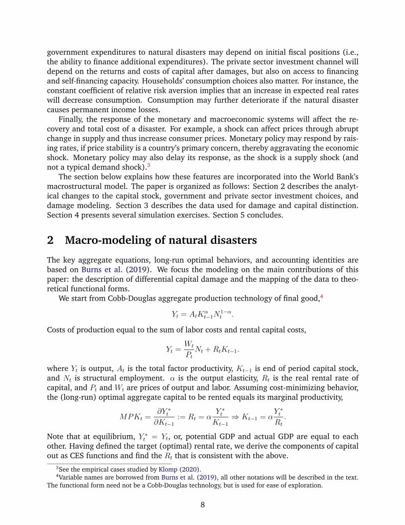
2.1 Capital stocks

Total capital stock is the sum of infrastructure capital (denoted with subscript S) and non-infrastructure capital (denoted with subscript N). Infrastructure and non-infrastructurecapital is derived from both private (denoted with subscript P ) and public capital (denotedwith subscript G). Given the equations above, we can derive solutions for both infrastruc-ture and non-infrastructure capital as well as a solution for the marginal product of capitalthat is consistent with aggregate capital. Figure 3 presents our main schema.

Figure 3: Schematic representation of the modeling of capital

We assume that capital is bundled together using a constant elasticity of substitutionassumption (CES), with several nests. This allows us to estimate the complementarity orsubstitutability of private and public capital in the provision of infrastructure and other cap-ital. This addition makes an important contribution - capital damages in infrastructure asan example may also make non-infrastructure capital inoperable (see examples discussedin Burns et al., 2020; Hallegatte and Vogt-Schilb, 2019). As an example, the CES calibrationfor infrastructure and other capital could ensure (a behavior close to) complementarities,while the nest for private and government capital could result in substitutes.

We assume that the economy is endowed with the following nested CES technology forthe aggregate capital,

Kt =[ω1K

ρ1S,t + ω2K

ρ1N,t

] 1ρ1 ,

for infrastructure,KS,t =

[ω3K

PS,t

ρ2+ ω4K

GS,t

ρ2] 1ρ2 ,

9

and non-infrastructureKN,t =

[ω5K

PN,t

ρ3+ ω6K

GN,t

ρ3] 1ρ3 .

where the share parameters for each capital (k) is denoted with ωi and the elasticity of sub-stitution σ = 1

1−ρis either estimated or calibrated. Assuming that the final good producer

minimizes its capital costs given the technology above, yields

RtKt−1 = RPS,tK

PS,t−1 +RG

S,tKGS,t−1︸ ︷︷ ︸

=RS,tKS,t−1

+RPN,tK

PN,t−1 +RG

N,tKGN,t−1︸ ︷︷ ︸

=RN,tKN,t−1

,

where the definitions of rental rates, Rs, follow the same logic as for aggregate capital andhence imply the equilibrium rates. As is standard in the literature, the first order conditionsfor infrastructure capital stock yield

∂Kt−1

∂KS,t−1

: RS,t = λt1

ρ1Kt−1

1−ρ1ρ1ω1Kρ1−1S,t−1,

with λ is a Langrangian. The rental rate for aggregate infrastructure becomes

RS,t = Kt−11−ρ1ω1K

ρ1−1S,t−1 = λtω1

(KS,t−1

Kt−1

)ρ1−1

.

Substituting the shadow cost value for marginal productivity of capital, i.e., λt = Rt,and solving for the optimal infrastructure capital stock KS,t yields,

KS,t−1 = ωσ11

(Rt

RS,t

)σ1

Kt−1,

Similarly, we solve for non-infrastructure capital,

KN,t−1 = ωσ12

(Rt

RN,t

)σ1

Kt−1.

In the same way we can write out the private and public optimal demands for bothinfrastructure and non-infrastructure capital,

KPS,t−1 = ωσ2

3

(RS,t

RPS,t

)σ2

KS,t−1,

KGS,t−1 = ωσ2

4

(RS,t

RGS,t

)σ2

KS,t−1,

KPN,t−1 = ωσ3

5

(RN,t

RPN,t

)σ3

KN,t−1,

KGN,t−1 = ωσ3

6

(RN,t

RGN,t

)σ3

KN,t−1.

10

The CES aggregator yields the aggregate optimal rental rate indices:

Rt =[ωσ11 RN,t

1−σ1 + ωσ12 RS,t

1−σ1] 1

1−σ1 ,

RS,t =[ωσ23 RP

S,t

1−σ2+ ωσ2

4 RGS,t

1−σ2] 1

1−σ2 ,

RN,t =[ωσ35 RP

N,t

1−σ3+ ωσ3

6 RGN,t

1−σ3] 1

1−σ3 .

Following Burns et al.’s (2019) modeling choices, each capital rental rate should be equalto its own long-term replacement cost. However, in the short run, the premium and/orsubsidies may differ due to certain rigidities. Therefore, the replacement cost is defined as

U ij,t =

P It (r

Bt + δt − πt + premt)

Pt(1− τCITt )

× ∂Kt−1

∂Kj,t−1

× ∂Kj,t−1

∂Kij,t−1

,

where i ∈ {P,G} and j ∈ {N,S}, δ is the capital depreciation rate, P It is the price of

investment and Pt is the domestic price, rBt is the risk-free rate (in this case the averageyield on government debt),5 premt is the risk-premium, πt is rate of inflation and τCIT

t isthe corporate tax rate.

The following no-arbitrage condition must hold in the long run,

Rij,t → U i

j,t + ε,

where the long-run level of the investment deflator converges to a constant ratio of theoutput deflator. In the short run, however, the growth rate of the investment deflator isa weighted average of nominal consumption inflation and its own lag, where the weightattached to past inflation, β, is estimated econometrically. Since there is no independentdata on price deflators for public investment as distinct from private investment, nor forproductive or adaptation investment, the four deflators are assumed to be equal

∆pi,jt = α + θ[pi,jt−1 − pC,XN

t−1

]+ β∆pi,jt−1 + (1− β)∆pC,XN

t + εPIt .

Note that all price indices are perfectly consistent with the aggregate capital stock from theproduction function and the different nests, as they have similar dynamics.

2.2 Investment decisions

The investment choices of the private and public sector are considered next.Our starting assumption is that real capital stock for private infrastructure evolves ac-

cording to a perpetual inventory method (hereafter; PIM),

KPS,t = (1− δ)KP

S,t−1 + IPS,t − IRPt .

Gross investments, IP , add to the existing capital stock net of depreciation, while recon-struction investments, IRP

t are diverting a fraction of new investment.

5Note that in Burns et al. (2019) the nominal interest rate was used as opposed to the average interest ondebt.

11

Private investment decisions depend on (i) adjustment costs; (ii) expected returns and(iii) short-run returns vs. short-run costs. The framework is based on Tobin’s Q, wherethe Q ratio is equal to the return to capital relative to the cost of capital (or market valueof assets to its replacement value). In this model, Tobin’s Q is defined as the ratio of themarginal product of capital to the cost of capital. The long run solves for the steady stateinvestment-capital ratio, which equals potential GDP growth, y∗t , plus the rate of capitaldepreciation, δ. The standard empirical private investment equation is written as

IPS,tKP

S,t−1

= β2

(∂Y ∗

t

∂KPS,t−1

− UPS,t − ε

)+ (1− β3)(∆y∗t + δ) + β3

IPS,t−1

KPS,t−2

+ εIPNt (1)

where εIPNt is an iid residual. We will discuss the marginal productivity of private

infrastructure capital shortly.Given that the modeling approach ensures that the investment variables, among others,

are on the same balanced growth path, and given that capital stocks are technologicallybound by the nested CES, it is easy to show that, in the long run, the following conditionis satisfied ∀j Ri

j,t → U ij,t + ε. Therefore, in the long run,

limt→+∞

αY ∗t

Kt−1

= limt→+∞

Ut

where Ut follows the same price aggregator as RTt .

2.3 Modeling of disaster channels

Given that the theoretical design of natural disasters is the same as climate change whencapital stocks are damaged, we use climate and natural disaster damages interchangeablyhenceforth. This section describes the aggregate damage functions for both public andprivate capital, and the channeling for disasters to the model.

Residual and gross damages are expressed in terms of the cost of rebuilding the dam-aged capital. For example, if a disaster destroys a road and the cost of rebuilding the roadis $1 million, then the official damage caused by the destruction of the road is $1 millionminus the usual capital depreciation rate.

Following Hallegatte and Vogt-Schilb’s (2019) main argument, simply subtracting thecost of rebuilding damage capital due to disasters from the total capital stock implies thatthe productivity of the destroyed capital was equal to the marginal product of the additionalcapital. In other words, capital remaining after the disaster can be reallocated instantlyand without cost to its most productive use. In reality, climate damages include both infra-marginal and marginal capital, and make capital reallocation only partially possible (e.g,bridges cannot be moved) because it takes time and is costly. It is important to note that theproductivity of infra-marginal capital is higher than that of marginal capital and thereforethe expected output loss would be higher. This is in fact an extension of the observation thatin the face of decreasing marginal productivity, average productivity will always be higherthan marginal productivity. Assuming that the damaged capital is evenly distributed acrosssub-marginal projects, the economic value of the destroyed capital is equal to the averageproductivity of capital.

12

Capital destroyed by disasters has approximately average capital productivity, whilenewly constructed capital has marginal productivity. Following Hallegatte et al. (2007), toproperly estimate the economic effects of climate damage it is necessary to keep track ofun-repaired climate damage, DSt, and calculate its economic effect separately from newincremental capital projects. Building on Burns et al. (2020), the stock of un-repairedclimate damage can be tracked using the following equation (we provide equations for theprivate sector, P , only, the public sector follows the same rationale),

DSPt = (1− δ)DSP

t−1 +RDPt − IRP

t ,

where RDPt is the residual damage (the gross damage net of the protection provided by the

adaptive investment) and IRPt is the investment in repairing damages (past and present,

indifferently) at time t, where repairs are equal to a constant share, ϕ, of the total invest-ment or total capital destroyed, whichever is smaller.

During the reconstruction phase, substitution and reallocation of infrastructure assetsare limited (Hallegatte and Vogt-Schilb, 2019) and we assume that the damaged capitalalters potential real production as follows

Y ∗t =

(KLt−1

KS,t−1

)AtN

αt K

1−αt−1︸ ︷︷ ︸

:=Yt

,

where KLt :=[ω3(K

PS,t −DSP

t )ρ2 + ω4(K

GS,t −DSG

t )ρ2] 1

ρ2 is the aggregation of both publicand private though the same technology as capital. This functional form is chosen for thefollowing properties: assuming that all capital is destroyed, there is no potential output. Ifhalf of the capital is destroyed proportionally between the private and the public, then po-tential output is halved. Note that when a natural disaster occurs, marginal productivitiesare affected, influencing investment choices.

This framework is consistent with the intuitions of Hallegatte and Vogt-Schilb (2019)as reparation will always be preferred to building new capital (see Appendix 7.2 for theproof).

Given that we have now defined real potential output, we are able to derive how dam-ages enter the investment decisions of the private sector. Specifically, we write the marginalproduct of private sector infrastructure capital

∂Y ∗t

∂KPS,t−1

= αY ∗t

Kt−1

∂Kt−1

∂KS,t−1

∂KS,t−1

∂KPS,t−1

+ ω3Yt

KS,t−1

( KLt−1

KPS,t −DSP

t

)1−ρ2

− Y ∗t

Yt

(KS,t−1

KPS,t−1

)1−ρ2 .

Hence large damages to capital relative to output (weighted by the product of the aggre-gate infrastructure and private infrastructure capital share and the substitution elasticity)may generate large increases in the marginal product of the damaged capital, throughDSt−1 and Y ∗

t . Interestingly, non-infrastructure capital marginal productivity will take theform

∂Y ∗t

∂KPN,t−1

= αY ∗t

Kt−1

∂Kt−1

∂KN,t−1

∂KN,t−1

∂KPS,t−1

.

Turning to investment in reconstruction, given that the capital destroyed by climatedisasters has approximately an average capital productivity, it would be optimal to direct

13

all investment to reconstruction. However, agency problems (not all investors will ownthe damaged capital) and regional and sectoral capacity constraints will prevent this out-come from being observed. To reflect these considerations, it is assumed that rebuildinginvestment cannot exceed a ϕ(t) share of total investment,

IRPt = min

((1− δ)DSP

t−1 +RDPt , ϕI

PS,t

). (2)

We assume that the ϕ is constant and equals 5%.Note that the model does not rule out total capital destruction. However, it is not

realistic to assume that all capital will be destroyed even in the case of a massive disaster.We therefore assume that about 10% of the capital is indestructible,

DSt = min(DSt−1 +RDt − IRt , 0.9Kt)

Further note that the model ignores the responses of labor productivity and humancapital to natural disasters. The model may also underestimate the actual impact of naturaldisasters given the rebuilding time.

2.4 Data and estimation

The macroeconomic model is estimated using the methodology presented in Burns andJooste (2019).

The production function technology is assumed to have a Cobb-Douglas form. Capital isaggregated using a CES function, with our main elasticity of interest being σT , which mea-sures the substitution between infrastructure and non-infrastructure capital. This parame-ter is important for computing the changes to the marginal product of capital, and hence tothe profitability of firms, to natural disasters. The productivity of non-infrastructure capitalwill rise or fall in line with an increase or decrease in infrastructure productivity if the twocapital variables are complements.

To estimate this parameter, we collect data on investment and capital stock from severalsources. The World Bank produces aggregate data on investment, private investment, andpublic investment for several countries in the Macro Poverty Outlook. The global PENNtables, discussed above, also include data on capital based on structures and non-structuresand their prices, which allows for a rough estimate of the elasticity of substitution.

Using panel estimation with standard fixed effects, we estimate a simple elasticity ofsubstitution using data on the ratio of infrastructure capital to non-infrastructure capi-tal as a function of the relative price of non-infrastructure capital to infrastructure capi-tal, ln

(KS

KN

)≈ αi + σT ln

(UN

US

). The elasticity is statistically significant and equals σT =

0.58(0.03), which implies that structures and non-infrastructure capital are complements.Indeed, given that σT = 1

1−ρ1, if ρ1 → −∞ then the function approaches a Leontief produc-

tion function.Unfortunately, data availability does not allow us to estimate the elasticity of substitu-

tion between private and public infrastructure or between private and public capital outsideinfrastructure. We assume that they are substitutes and set σS(ρ2) = σN(ρ3) = 2.6

6For other estimates of aggregate capital substitution between the private and government sector, see Anet al. (2019).

14

3 Macroeconomic impact of a natural disaster

We start by generating a model-determined baseline without shocks for 200 periods, i.e.,200 years, that we identify as the steady state.7 We then proceed to introduce shocksrelative to the steady state baseline. This setting allows us to reduce the influence of short-term deviation impacts from the balance growth path for the shock analysis.

In this section, we compare results for different disaster sizes, ranging from 1% to20% loss of the infrastructure. While the largest disaster is perhaps unrealistically large,it illustrates several useful properties of the model. We also reproduce a disaster of amagnitude similar to the 1999 Marmara Earthquake, as one example of large plausibleshock. The next set of simulations draw from the empirical distribution using the GEMdata to extract uncertainty intervals for the economic outcomes and to assess potentiallosses from realized data.

3.1 Economic response after a natural disaster

Throughout the simulations, results are displayed relative to the baseline in which shocksand resilience strategies are absent from the analysis. The natural disaster shock is intro-duced in year three, discussed shortly.

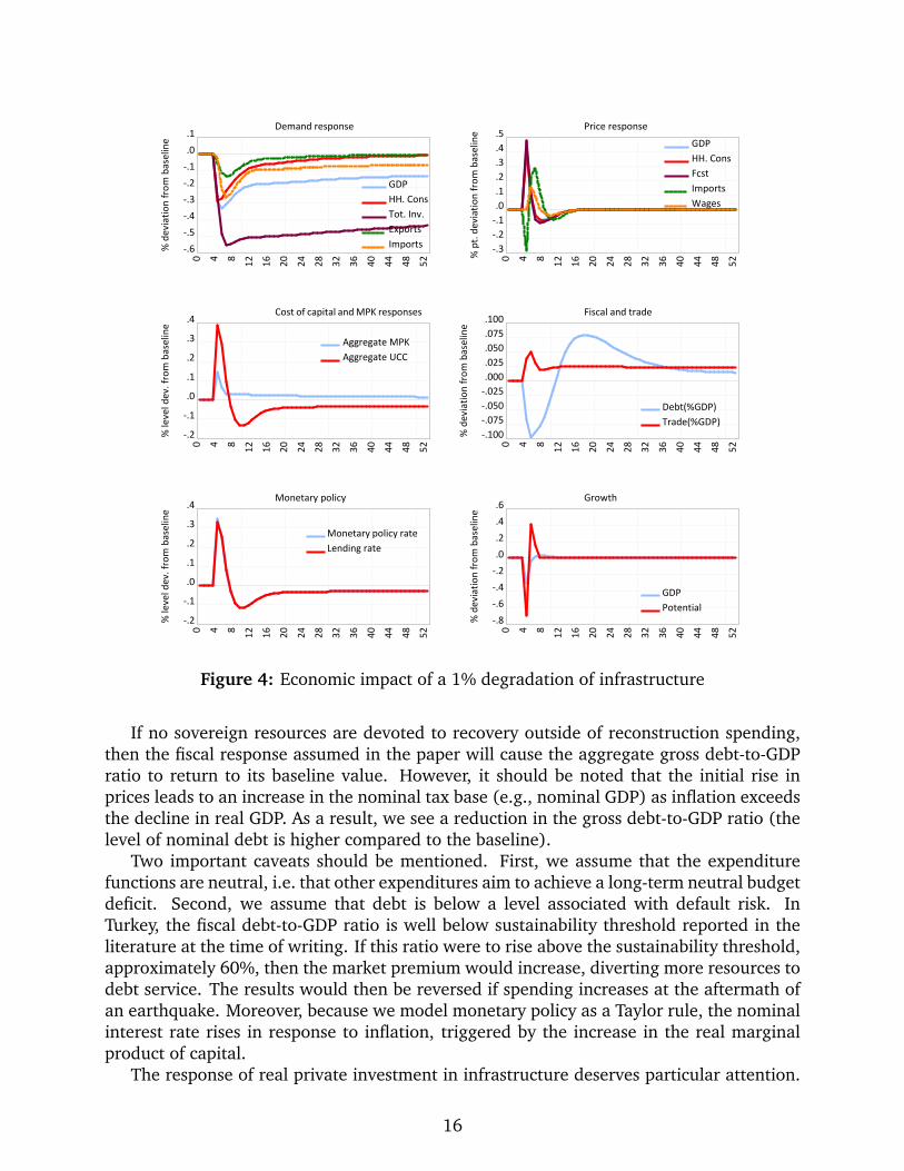
In the scenario showed in figure 4, the physical damages from the disasters are fully re-paired within three year. However, the consequences of the disasters are almost permanentin levels. The top left hand side panel shows that real GDP, consumption, and investmentfall after the shock. The shock also generates inflation (top panel on the right), whichdegenerates back to the baseline level for a decade after the shock. The largest increasein inflation occurs after the shock. The inflation response is mainly due to a cost-pushmechanism, following a co-mutual increase in the rental rate of capital and in the outputgap (potential output falls faster than actual output). Real demand does fall, but less thanpotential, leading to an inflationary response. One may also view this in the context offactor prices. The rental rate of capital increases when capital is destroyed (supply of capi-tal falls relative to demand). The impact on wages is complicated given the existence of awage-price loop.

This modeling result can be compared with empirical findings on most natural disas-ters that report increased inflation after climate shocks (see e.g., Parker, 2018). However,empirical results for the case of earthquakes remain inconclusive. Cavallo et al. (2014)studies the impacts of the 2010 Chilean and the 2011 Japanese earthquakes and show thatshortages at the aftermath of these events did not translate into higher prices. Moreover,Doyle and Noy (2015) showed that the Canterbury earthquake in 2010 generated a fall inaggregate demand that decreased prices (note that the results were insignificant). How-ever, the Canterbury earthquakes are not a great example for drawing wider conclusionssince the rate of insurance was high (Wood et al., 2016). Furthermore, using global data,Parker (2018) shows that earthquakes increase the price of energy, clothing and footwear,while food prices seem to have declined in the first few quarters after the shock. Morerecently, using a simultaneous equation model with global data, Klomp (2020) finds apositive response of inflation after the occurrence of an earthquake.

7See Figure 17 in the appendix.

15

-.6-.5-.4-.3-.2-.1.0.1

0 4 8 12 16 20 24 28 32 36 40 44 48 52

GDPHH. ConsTot. Inv.ExportsImports%

dev

iatio

n fro

m b

asel

ine

Demand response

-.3-.2-.1.0.1.2.3.4.5

0 4 8 12 16 20 24 28 32 36 40 44 48 52

GDPHH. ConsFcstImportsWages

% p

t. de

viat

ion

from

bas

elin

e

Price response

-.2

-.1

.0

.1

.2

.3

.4

0 4 8 12 16 20 24 28 32 36 40 44 48 52

Aggregate MPKAggregate UCC

% le

vel d

ev. f

rom

bas

elin

e

Cost of capital and MPK responses

-.100-.075-.050-.025.000.025.050.075.100

0 4 8 12 16 20 24 28 32 36 40 44 48 52

Debt(%GDP)Trade(%GDP)

% d

evia

tion

from

bas

elin

e

Fiscal and trade

-.2

-.1

.0

.1

.2

.3

.4

0 4 8 12 16 20 24 28 32 36 40 44 48 52

Monetary policy rateLending rate

% le

vel d

ev. f

rom

bas

elin

e

Monetary policy

-.8-.6-.4-.2.0.2.4.6

0 4 8 12 16 20 24 28 32 36 40 44 48 52

GDPPotential

% d

evia

tion

from

bas

elin

e

Growth

Figure 4: Economic impact of a 1% degradation of infrastructure

If no sovereign resources are devoted to recovery outside of reconstruction spending,then the fiscal response assumed in the paper will cause the aggregate gross debt-to-GDPratio to return to its baseline value. However, it should be noted that the initial rise inprices leads to an increase in the nominal tax base (e.g., nominal GDP) as inflation exceedsthe decline in real GDP. As a result, we see a reduction in the gross debt-to-GDP ratio (thelevel of nominal debt is higher compared to the baseline).

Two important caveats should be mentioned. First, we assume that the expenditurefunctions are neutral, i.e. that other expenditures aim to achieve a long-term neutral budgetdeficit. Second, we assume that debt is below a level associated with default risk. InTurkey, the fiscal debt-to-GDP ratio is well below sustainability threshold reported in theliterature at the time of writing. If this ratio were to rise above the sustainability threshold,approximately 60%, then the market premium would increase, diverting more resources todebt service. The results would then be reversed if spending increases at the aftermath ofan earthquake. Moreover, because we model monetary policy as a Taylor rule, the nominalinterest rate rises in response to inflation, triggered by the increase in the real marginalproduct of capital.

The response of real private investment in infrastructure deserves particular attention.

16

Although the marginal product of capital is higher than the cost of capital in the medium-term, investment after a disaster is below the baseline. This is primarily driven by theinvestment equation (Eq. 1). The investment choices include the remaining capital, takinginto account the reconstruction and adjustment investments of the previous period. Thecombination of lower expected real income and the inertia of the investment decision im-plies that the increase in investment due to the marginal product of capital is completelyoffset in subsequent periods. In turn, the government’s investment response (those not de-voted to reconstruction) is assumed to hit a fixed share of fiscal revenues to maintain bud-get neutrality (a modeling assumption not necessarily reflecting historical fiscal responsesby Turkey). Taxes, and thus government spending decisions, are sensitive to movements inthe tax base, which is itself sensitive to the degree of price rigidity. Sticky prices and activemonetary policy can further reduce output after a natural disaster shock. Such a scenariomay lead to a large increase in the user cost of capital (larger than the return to capital),which reduces the expected profits from investing in the short- to medium-term. We willfurther discuss the role that the monetary policy plays shortly.

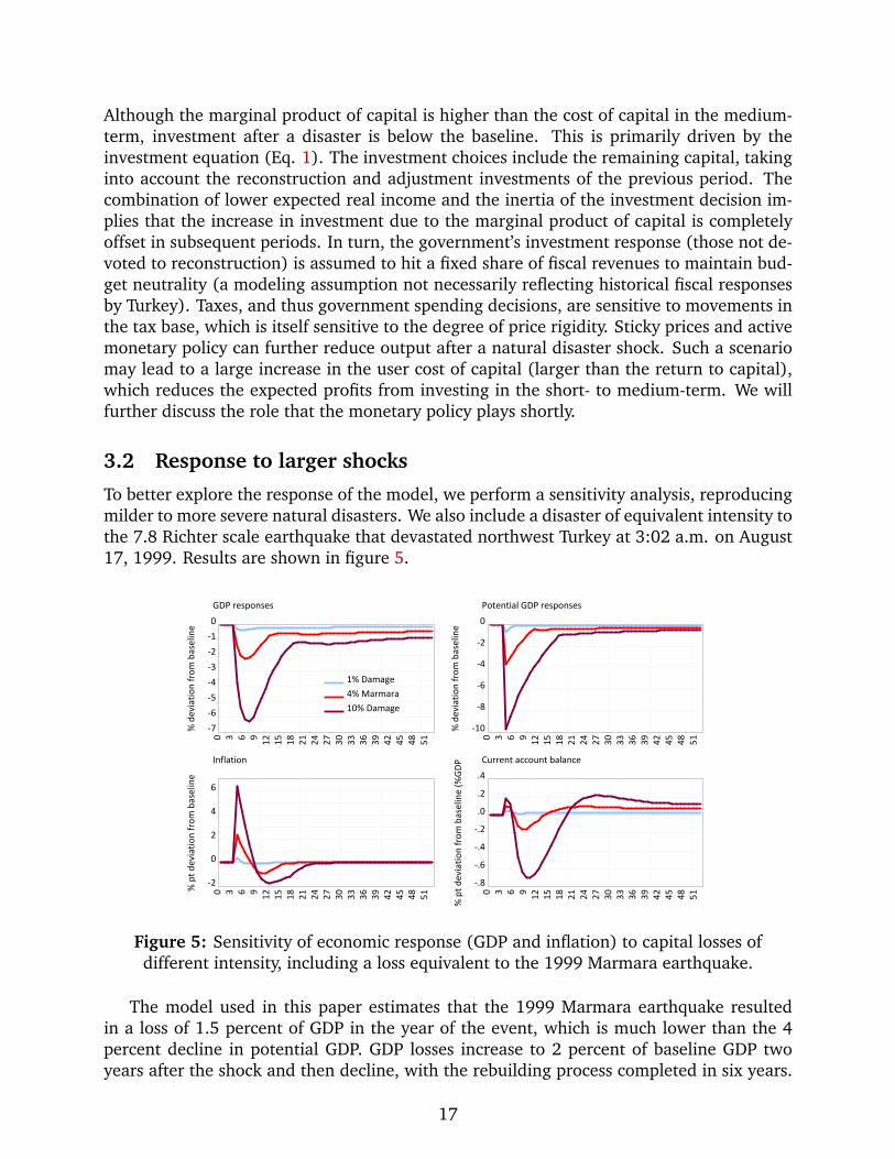
3.2 Response to larger shocks

To better explore the response of the model, we perform a sensitivity analysis, reproducingmilder to more severe natural disasters. We also include a disaster of equivalent intensity tothe 7.8 Richter scale earthquake that devastated northwest Turkey at 3:02 a.m. on August17, 1999. Results are shown in figure 5.

-7-6-5-4-3-2-10

0 3 6 9 12 15 18 21 24 27 30 33 36 39 42 45 48 51

1% Damage4% Marmara10% Damage

% d

evia

tion

from

bas

elin

e

GDP responses

-10

-8

-6

-4

-2

0

0 3 6 9 12 15 18 21 24 27 30 33 36 39 42 45 48 51

% d

evia

tion

from

bas

elin

e

Potential GDP responses

-2

0

2

4

6

0 3 6 9 12 15 18 21 24 27 30 33 36 39 42 45 48 51

% p

t dev

iatio

n fro

m b

asel

ine

Inflation

-.8

-.6

-.4

-.2

.0

.2

.4

0 3 6 9 12 15 18 21 24 27 30 33 36 39 42 45 48 51% p

t dev

iatio

n fro

m b

asel

ine

(%GD

P Current account balance

Figure 5: Sensitivity of economic response (GDP and inflation) to capital losses ofdifferent intensity, including a loss equivalent to the 1999 Marmara earthquake.

The model used in this paper estimates that the 1999 Marmara earthquake resultedin a loss of 1.5 percent of GDP in the year of the event, which is much lower than the 4percent decline in potential GDP. GDP losses increase to 2 percent of baseline GDP twoyears after the shock and then decline, with the rebuilding process completed in six years.

17

The earthquake occurred during an economic recession that makes it difficult to quantifyempirically the GDP losses. For comparison, a model-based simulation done after the event(World Bank, 1999) suggested immediate losses amounting to 0.6 to 1 percent of GDP.

These results show that the economic response is not linear: the model response isdifferent for small and large shocks. This nonlinearity is, in part, determined by equation2 as well as the interaction of the output gap on prices and interest rates. These responsesof inflation illustrate this point, with a more complex dynamics for larger shocks.

Two additional points are worth mentioning. First, while supply (i.e. potential GDP)reacts strongly to large shocks, economic mechanisms and dynamics smooth and delay theeconomic response, giving GDP responses their curvature. Second, the V-shaped responseof potential GDP reflects the recovery process of investment in the economy. While ittakes about three years to recover from a 1% loss in the capital stock, the recovery periodsincrease to six and fourteen years respectively for a Marmara-sized shock and a 10% shock.

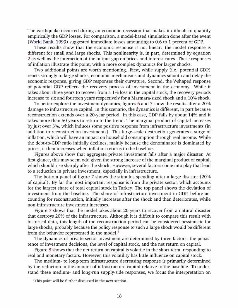
To better explore the investment dynamics, figures 6 and 7 show the results after a 20%damage to infrastructure capital. In this scenario, the dynamics is different, in part becausereconstruction extends over a 20-year period. In this case, GDP falls by about 14% and ittakes more than 50 years to return to the trend. The marginal product of capital increasesby just over 5%, which induces some positive response from infrastructure investments (inaddition to reconstruction investments). This large-scale destruction generates a surge ofinflation, which will have an impact on household consumption through real income. Whilethe debt-to-GDP ratio initially declines, mainly because the denominator is dominated byprices, it then increases when inflation returns to the baseline.

Figures above show that aggregate private investment falls after a major disaster. Atfirst glance, this may seem odd given the strong increase of the marginal product of capital,which should rise sharply after the shock. However, several factors come into play that leadto a reduction in private investment, especially in infrastructure.

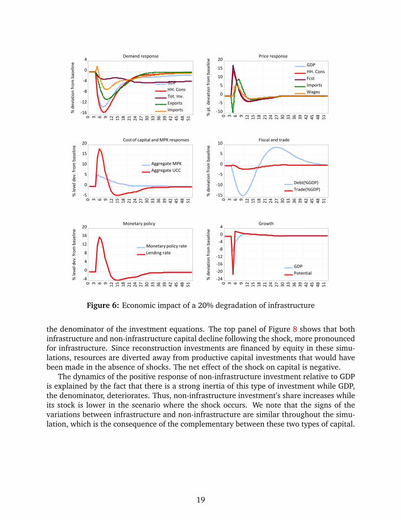
The bottom panel of figure 7 shows the stimulus spending after a large disaster (20%of capital). By far the most important response is from the private sector, which accountsfor the largest share of total capital stock in Turkey. The top panel shows the deviation ofinvestment from the baseline. The share of infrastructure investment in GDP, before ac-counting for reconstruction, initially increases after the shock and then deteriorates, whilenon-infrastructure investment increases.

Figure 7 shows that the model takes about 20 years to recover from a natural disasterthat destroys 20% of the infrastructure. Although it is difficult to compare this result withhistorical data, this length of the reconstruction period can be considered pessimistic forlarge shocks, probably because the policy response to such a large shock would be differentfrom the behavior represented in the model.8

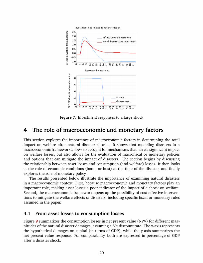
The dynamics of private sector investment are determined by three factors: the persis-tence of investment decisions, the level of capital stock, and the net return on capital.

Figure 8 shows that the net return on capital is volatile in the short-term, responding toreal and monetary factors. However, this volatility has little influence on capital stock.

The medium- to long-term infrastructure decreasing response is primarily determinedby the reduction in the amount of infrastructure capital relative to the baseline. To under-stand these medium- and long-run supply-side responses, we focus the interpretation on

8This point will be further discussed in the next section.

18

-16

-12

-8

-4

0

4

0 3 6 9 12 15 18 21 24 27 30 33 36 39 42 45 48 51

GDPHH. ConsTot. Inv.ExportsImports%

dev

iatio

n fro

m b

asel

ine

Demand response

-10

-5

0

5

10

15

20

0 3 6 9 12 15 18 21 24 27 30 33 36 39 42 45 48 51

GDPHH. ConsFcstImportsWages

% p

t. de

viat

ion

from

bas

elin

e Price response

-5

0

5

10

15

20

0 3 6 9 12 15 18 21 24 27 30 33 36 39 42 45 48 51

Aggregate MPKAggregate UCC

% le

vel d

ev. f

rom

bas

elin

e

Cost of capital and MPK responses

-15

-10

-5

0

5

10

0 3 6 9 12 15 18 21 24 27 30 33 36 39 42 45 48 51

Debt(%GDP)Trade(%GDP)

% d

evia

tion

from

bas

elin

e

Fiscal and trade

-4

0

4

8

12

16

20

0 3 6 9 12 15 18 21 24 27 30 33 36 39 42 45 48 51

Monetary policy rateLending rate

% le

vel d

ev. f

rom

bas

elin

e

Monetary policy

-24-20-16-12

-8-404

0 3 6 9 12 15 18 21 24 27 30 33 36 39 42 45 48 51

GDPPotential

% d

evia

tion

from

bas

elin

e

Growth

Figure 6: Economic impact of a 20% degradation of infrastructure

the denominator of the investment equations. The top panel of Figure 8 shows that bothinfrastructure and non-infrastructure capital decline following the shock, more pronouncedfor infrastructure. Since reconstruction investments are financed by equity in these simu-lations, resources are diverted away from productive capital investments that would havebeen made in the absence of shocks. The net effect of the shock on capital is negative.

The dynamics of the positive response of non-infrastructure investment relative to GDPis explained by the fact that there is a strong inertia of this type of investment while GDP,the denominator, deteriorates. Thus, non-infrastructure investment’s share increases whileits stock is lower in the scenario where the shock occurs. We note that the signs of thevariations between infrastructure and non-infrastructure are similar throughout the simu-lation, which is the consequence of the complementary between these two types of capital.

19

-1.0-0.50.00.51.01.52.02.5

0 3 6 9 12 15 18 21 24 27 30 33 36 39 42 45 48 51

Infrastructure investmentNon-infrastructure investment

% G

DP d

evia

tion

from

bas

elin

e

Investment not related to reconstruction

.0

.2

.4

.6

.80 3 6 9 12 15 18 21 24 27 30 33 36 39 42 45 48 51

PrivateGovernment

% G

DP d

evia

tion

from

bas

elin

eRecovery investment

Figure 7: Investment responses to a large shock

4 The role of macroeconomic and monetary factors

This section explores the importance of macroeconomic factors in determining the totalimpact on welfare after natural disaster shocks. It shows that modeling disasters in amacroeconomic framework allows to account for mechanisms that have a significant impacton welfare losses, but also allows for the evaluation of macrofiscal or monetary policiesand options that can mitigate the impact of disasters. The section begins by discussingthe relationship between asset losses and consumption (and welfare) losses. It then looksat the role of economic conditions (boom or bust) at the time of the disaster, and finallyexplores the role of monetary policy.

The results presented below illustrate the importance of examining natural disastersin a macroeconomic context. First, because macroeconomic and monetary factors play animportant role, making asset losses a poor indicator of the impact of a shock on welfare.Second, the macroeconomic framework opens up the possibility of cost-effective interven-tions to mitigate the welfare effects of disasters, including specific fiscal or monetary rulesassumed in the paper.

4.1 From asset losses to consumption losses

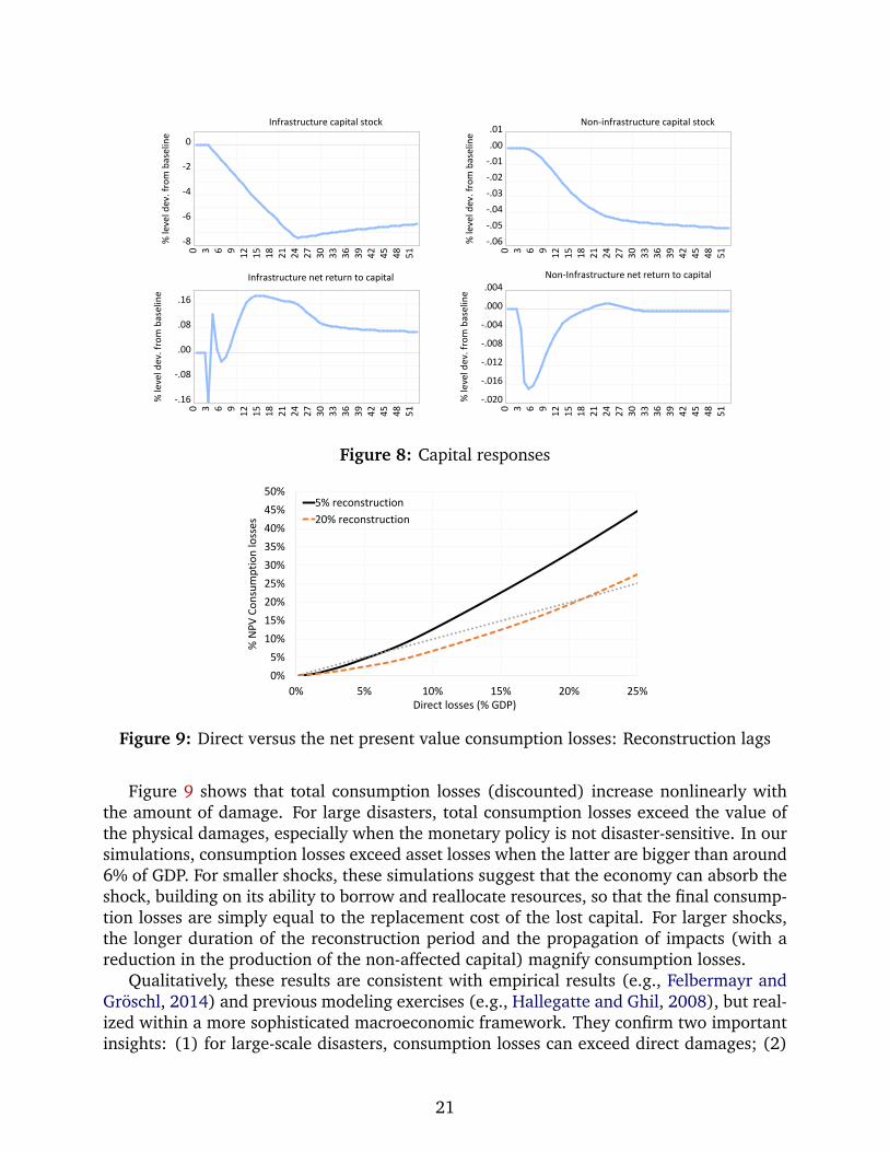
Figure 9 summarizes the consumption losses in net present value (NPV) for different mag-nitudes of the natural disaster damages, assuming a 6% discount rate. The x-axis representsthe hypothetical damages on capital (in terms of GDP), while the y-axis summarizes thenet present value response. For comparability, both are expressed in percentage of GDPafter a disaster shock.

20

-8

-6

-4

-2

0

0 3 6 9 12 15 18 21 24 27 30 33 36 39 42 45 48 51

% le

vel d

ev. f

rom

bas

elin

e

Infrastructure capital stock

-.06-.05-.04-.03-.02-.01.00.01

0 3 6 9 12 15 18 21 24 27 30 33 36 39 42 45 48 51

% le

vel d

ev. f

rom

bas

elin

e

Non-infrastructure capital stock

-.16

-.08

.00

.08

.16

0 3 6 9 12 15 18 21 24 27 30 33 36 39 42 45 48 51

% le

vel d

ev. f

rom

bas

elin

e

Infrastructure net return to capital

-.020

-.016

-.012

-.008

-.004

.000

.004

0 3 6 9 12 15 18 21 24 27 30 33 36 39 42 45 48 51

% le

vel d

ev. f

rom

bas

elin

e

Non-Infrastructure net return to capital

Figure 8: Capital responses

0%

5%

10%

15%

20%

25%

30%

35%

40%

45%

50%

0% 5% 10% 15% 20% 25%

% N

PV

Co

nsu

mp

tio

n lo

sses

Direct losses (% GDP)

5% reconstruction

20% reconstruction

Figure 9: Direct versus the net present value consumption losses: Reconstruction lags

Figure 9 shows that total consumption losses (discounted) increase nonlinearly withthe amount of damage. For large disasters, total consumption losses exceed the value ofthe physical damages, especially when the monetary policy is not disaster-sensitive. In oursimulations, consumption losses exceed asset losses when the latter are bigger than around6% of GDP. For smaller shocks, these simulations suggest that the economy can absorb theshock, building on its ability to borrow and reallocate resources, so that the final consump-tion losses are simply equal to the replacement cost of the lost capital. For larger shocks,the longer duration of the reconstruction period and the propagation of impacts (with areduction in the production of the non-affected capital) magnify consumption losses.

Qualitatively, these results are consistent with empirical results (e.g., Felbermayr andGroschl, 2014) and previous modeling exercises (e.g., Hallegatte and Ghil, 2008), but real-ized within a more sophisticated macroeconomic framework. They confirm two importantinsights: (1) for large-scale disasters, consumption losses can exceed direct damages; (2)

21

macrofiscal and monetary policies can play in important role in mitigating the impact oflarge disasters.

In the case of Turkey, our model suggests that the threshold level at which consumptionlosses exceed asset losses is high, and the nonlinearity is low. At 6% of GDP in the baselinescenario, this threshold is higher than the most severe floods and earthquakes that are mostlikely in the probability distributions considered in the next sections of the paper.

This result should be viewed with caution, however, as this threshold will depend ona few parameters that are difficult to estimate, such as the economy’s ability to mobilizeresources for reconstruction. Figure 9 illustrates this point. By increasing the capacity tomobilize (or divert) resources for reconstruction, changing the parameter ϕ in eq. 2 from5% to 20%, the threshold increases from 6% to 21%. The faster the economy is able torebuild, the less welfare is lost.

4.2 The importance of the economic situation before the shock

The previous simulations were performed on a steady state growth path, but disasters affecteconomies at specific phases of their business cycle. For example, the Marmara earthquakeaffected Turkey during a recession. However, the economic response to a shock is not likelyto be similar: in particular, the increase in demand created by reconstruction is less likely todisplace workers and production capacity during a recession than during an expansion. Inaddition, the demand created by reconstruction can act as a stimulus, boosting aggregatedemand and accelerating the macroeconomic recovery and reconstruction process. Forexample, the 1992 Hurricane Andrew hit Florida when half of the construction workers inthe state were unemployed.

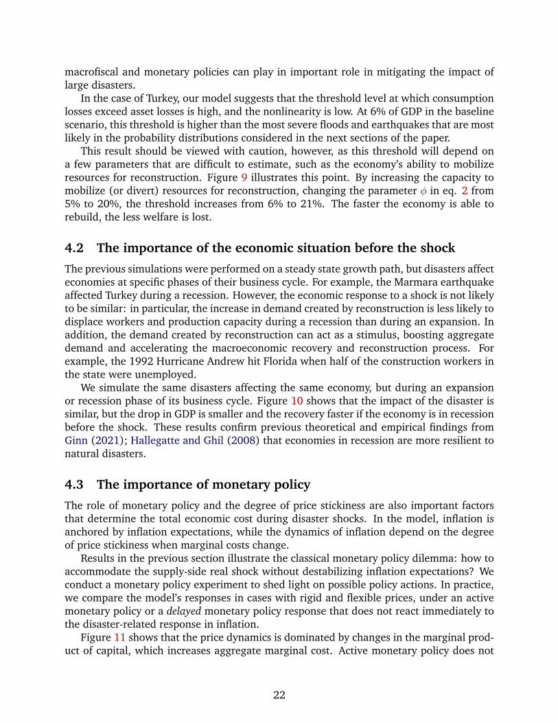
We simulate the same disasters affecting the same economy, but during an expansionor recession phase of its business cycle. Figure 10 shows that the impact of the disaster issimilar, but the drop in GDP is smaller and the recovery faster if the economy is in recessionbefore the shock. These results confirm previous theoretical and empirical findings fromGinn (2021); Hallegatte and Ghil (2008) that economies in recession are more resilient tonatural disasters.

4.3 The importance of monetary policy

The role of monetary policy and the degree of price stickiness are also important factorsthat determine the total economic cost during disaster shocks. In the model, inflation isanchored by inflation expectations, while the dynamics of inflation depend on the degreeof price stickiness when marginal costs change.

Results in the previous section illustrate the classical monetary policy dilemma: how toaccommodate the supply-side real shock without destabilizing inflation expectations? Weconduct a monetary policy experiment to shed light on possible policy actions. In practice,we compare the model’s responses in cases with rigid and flexible prices, under an activemonetary policy or a delayed monetary policy response that does not react immediately tothe disaster-related response in inflation.

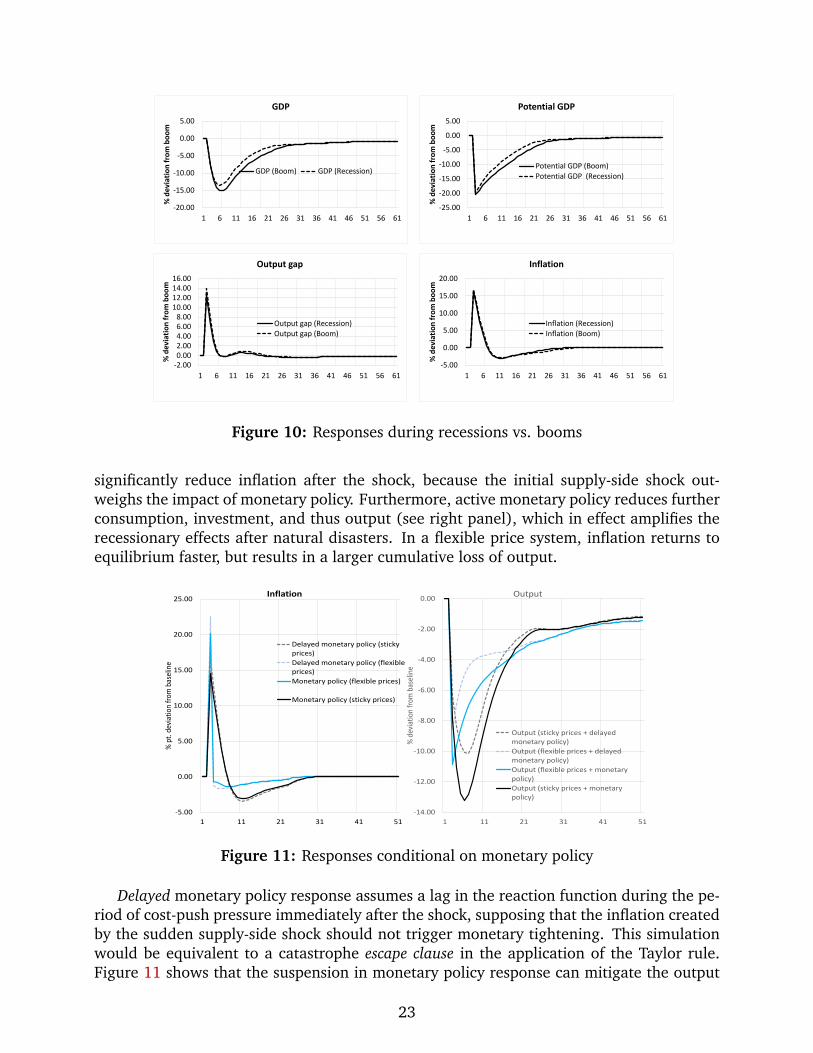
Figure 11 shows that the price dynamics is dominated by changes in the marginal prod-uct of capital, which increases aggregate marginal cost. Active monetary policy does not

22

-20.00

-15.00

-10.00

-5.00

0.00

5.00

1 6 11 16 21 26 31 36 41 46 51 56 61

% d

evia

tio

n f

rom

bo

om

GDP

GDP (Boom) GDP (Recession)

-25.00

-20.00

-15.00

-10.00

-5.00

0.00

5.00

1 6 11 16 21 26 31 36 41 46 51 56 61

% d

evia

tio

n f

rom

bo

om

Potential GDP

Potential GDP (Boom)Potential GDP (Recession)

-2.000.002.004.006.008.00

10.0012.0014.0016.00

1 6 11 16 21 26 31 36 41 46 51 56 61

% d

evia

tio

n f

rom

bo

om

Output gap

Output gap (Recession)Output gap (Boom)

-5.00

0.00

5.00

10.00

15.00

20.00

1 6 11 16 21 26 31 36 41 46 51 56 61

% d

evia

tio

n f

rom

bo

om

Inflation

Inflation (Recession)Inflation (Boom)

Figure 10: Responses during recessions vs. booms

significantly reduce inflation after the shock, because the initial supply-side shock out-weighs the impact of monetary policy. Furthermore, active monetary policy reduces furtherconsumption, investment, and thus output (see right panel), which in effect amplifies therecessionary effects after natural disasters. In a flexible price system, inflation returns toequilibrium faster, but results in a larger cumulative loss of output.

-14.00

-12.00

-10.00

-8.00

-6.00

-4.00

-2.00

0.00

1 11 21 31 41 51

% d

evia

tion

from

bas

elin

e

Output

Output (sticky prices + delayedmonetary policy)

Output (flexible prices + delayedmonetary policy)

Output (flexible prices + monetarypolicy)

Output (sticky prices + monetarypolicy)

-5.00

0.00

5.00

10.00

15.00

20.00

25.00

1 11 21 31 41 51

% p

t. d

evia

tion

from

bas

elin

e

Inflation

Delayed monetary policy (stickyprices)

Delayed monetary policy (flexibleprices)

Monetary policy (flexible prices)

Monetary policy (sticky prices)

Figure 11: Responses conditional on monetary policy

Delayed monetary policy response assumes a lag in the reaction function during the pe-riod of cost-push pressure immediately after the shock, supposing that the inflation createdby the sudden supply-side shock should not trigger monetary tightening. This simulationwould be equivalent to a catastrophe escape clause in the application of the Taylor rule.Figure 11 shows that the suspension in monetary policy response can mitigate the output

23

and consumption impact significantly, without generating large trade-off with long-terminflation.

Our findings are aligned with past monetary policy practices reported in Klomp (2020)in the context of earthquakes. This paper shows that the policy interest rate drops in thefirst year after an earthquake, meaning that monetary authorities prioritized recovery overprice stability. The plausible explanation provided by the author is that demand shocks aremore likely to dominate supply shocks, which echoes the result of our simulations whenwe compare actual and potential GDP growth rates (see Figure 6).

These results call for more research on the design of monetary policy in post-disasterand crisis situations, a topic with considerable uncertainty. As an example, Ehrmann andSmets (2003) explore the economic consequences when monetary policy reacts to incorrectinformation, and show that a more conservative approach (i.e., reducing the weight on theoutput gap in the interest rate reaction function) reduces the welfare loss from supply-sideshocks. And Ferrero et al. (2019) show that the uncertainty on the inflation response to theoutput gap should lead to a monetary policy response that is more aggressive for transientshocks and more cautious for permanent shocks.

Natural disasters are exogenous, short, and transitory shocks. They are therefore lesslikely to destabilize inflation expectations. In this particular case, our model suggests that atemporary suspension in monetary policy (i.e., not increasing rates immediately followinga natural disaster) helps the economy cope with the transient supply-side shock. However,in the context of climate change, when particular shocks become increasingly frequent,they may affect inflation expectations and a similar strategy may have unintended adverseeffects (Batten et al., 2016; Rudebusch et al., 2019). In the current Turkish context, itshould be recognized that inflation is historically high and that inflation expectations maynot be anchored and therefore sensitive to shocks under a loose monetary policy regime.

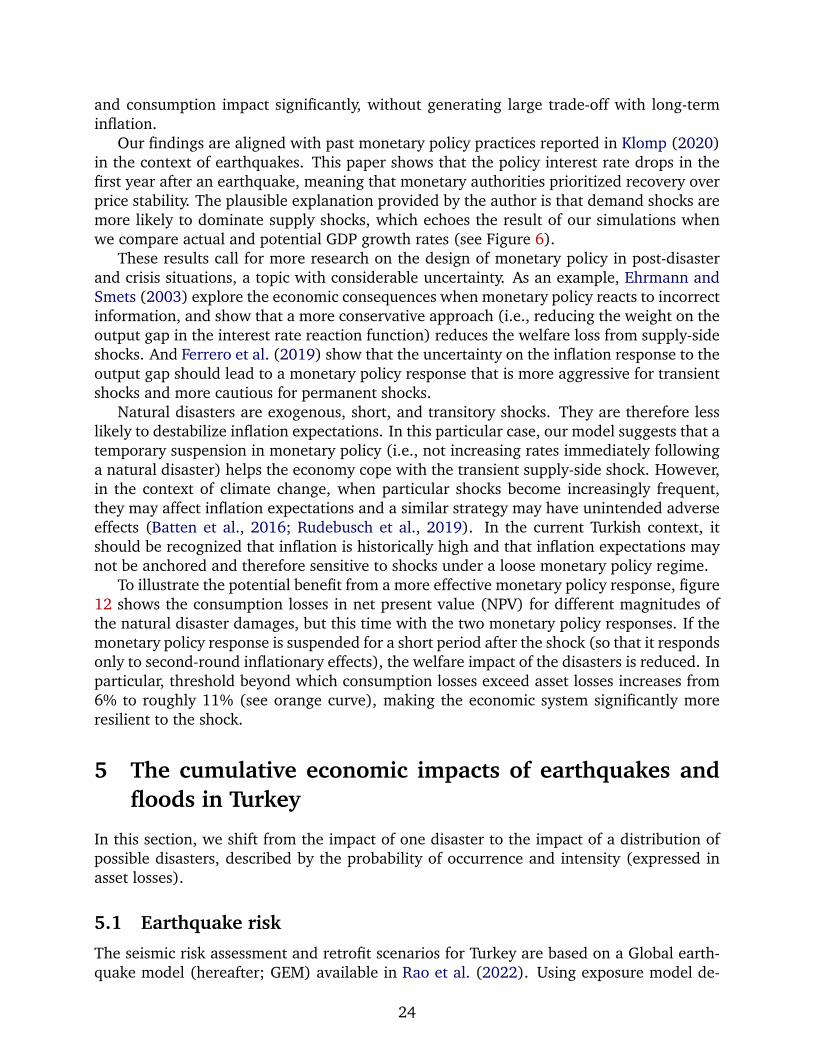
To illustrate the potential benefit from a more effective monetary policy response, figure12 shows the consumption losses in net present value (NPV) for different magnitudes ofthe natural disaster damages, but this time with the two monetary policy responses. If themonetary policy response is suspended for a short period after the shock (so that it respondsonly to second-round inflationary effects), the welfare impact of the disasters is reduced. Inparticular, threshold beyond which consumption losses exceed asset losses increases from6% to roughly 11% (see orange curve), making the economic system significantly moreresilient to the shock.

5 The cumulative economic impacts of earthquakes andfloods in Turkey

In this section, we shift from the impact of one disaster to the impact of a distribution ofpossible disasters, described by the probability of occurrence and intensity (expressed inasset losses).

5.1 Earthquake risk

The seismic risk assessment and retrofit scenarios for Turkey are based on a Global earth-quake model (hereafter; GEM) available in Rao et al. (2022). Using exposure model de-

24

0%

5%

10%

15%

20%

25%

30%

35%

40%

0% 5% 10% 15% 20%

% N

PV

Co

nsu

mp

tio

n lo

sses

Direct losses (% GDP)

Without MP suspension

With MP suspension

Figure 12: Direct versus the net present value consumption losses, with and withoutmonetary policy suspension

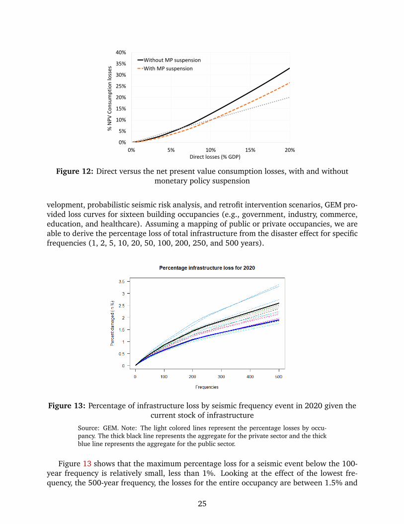
velopment, probabilistic seismic risk analysis, and retrofit intervention scenarios, GEM pro-vided loss curves for sixteen building occupancies (e.g., government, industry, commerce,education, and healthcare). Assuming a mapping of public or private occupancies, we areable to derive the percentage loss of total infrastructure from the disaster effect for specificfrequencies (1, 2, 5, 10, 20, 50, 100, 200, 250, and 500 years).

Figure 13: Percentage of infrastructure loss by seismic frequency event in 2020 given thecurrent stock of infrastructure

Source: GEM. Note: The light colored lines represent the percentage losses by occu-pancy. The thick black line represents the aggregate for the private sector and the thickblue line represents the aggregate for the public sector.

Figure 13 shows that the maximum percentage loss for a seismic event below the 100-year frequency is relatively small, less than 1%. Looking at the effect of the lowest fre-quency, the 500-year frequency, the losses for the entire occupancy are between 1.5% and

25

3.5%, with an average of about 1.8% for the public sector and 2.5% for the private sector.Since the private sector is much larger than the public sector in terms of buildings, theglobal average is close to that of the private sector.

Two caveats are worth mentioning. First, the disaster coverage is for buildings only.Therefore, simulations based on these data will not provide impacts on infrastructure, forexperiments with GEM infrastructure has to be understood as buildings. Second, theseresults are based on the 2013 Euro-Mediterranean seismic risk model. Early simulationsof the 2020 Euro-Mediterranean seismic risk model for Turkey may suggest higher overallimpacts.

A Monte Carlo simulation draws from the empirical cumulative distribution function,FX , using the empirical inverse probability integral transform, F−1

X (u) = x.9 Our simula-tions start in 2021 as opposed to the steady state simulations earlier.

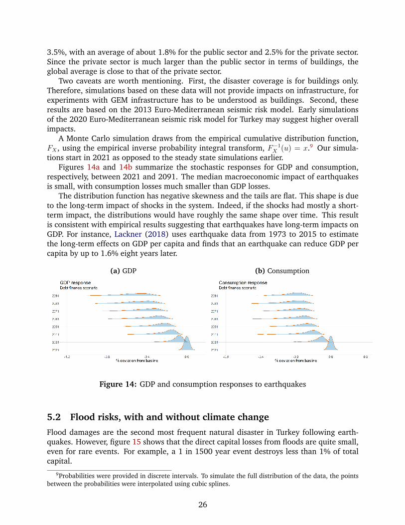
Figures 14a and 14b summarize the stochastic responses for GDP and consumption,respectively, between 2021 and 2091. The median macroeconomic impact of earthquakesis small, with consumption losses much smaller than GDP losses.

The distribution function has negative skewness and the tails are flat. This shape is dueto the long-term impact of shocks in the system. Indeed, if the shocks had mostly a short-term impact, the distributions would have roughly the same shape over time. This resultis consistent with empirical results suggesting that earthquakes have long-term impacts onGDP. For instance, Lackner (2018) uses earthquake data from 1973 to 2015 to estimatethe long-term effects on GDP per capita and finds that an earthquake can reduce GDP percapita by up to 1.6% eight years later.

(a) GDP (b) Consumption

Figure 14: GDP and consumption responses to earthquakes

5.2 Flood risks, with and without climate change

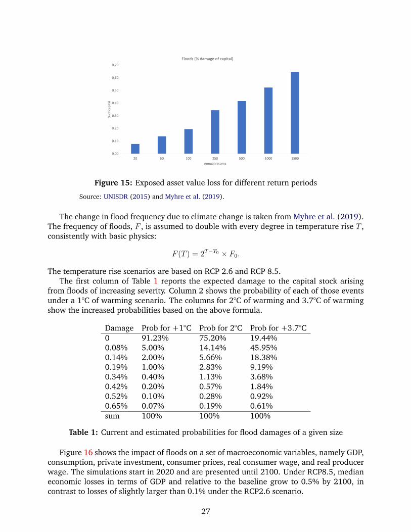
Flood damages are the second most frequent natural disaster in Turkey following earth-quakes. However, figure 15 shows that the direct capital losses from floods are quite small,even for rare events. For example, a 1 in 1500 year event destroys less than 1% of totalcapital.

9Probabilities were provided in discrete intervals. To simulate the full distribution of the data, the pointsbetween the probabilities were interpolated using cubic splines.

26

0.00

0.10

0.20

0.30

0.40

0.50

0.60

0.70

20 50 100 250 500 1000 1500

% o

f ca

pit

al

Annual returns

Floods (% damage of capital)

Figure 15: Exposed asset value loss for different return periods

Source: UNISDR (2015) and Myhre et al. (2019).

The change in flood frequency due to climate change is taken from Myhre et al. (2019).The frequency of floods, F , is assumed to double with every degree in temperature rise T ,consistently with basic physics:

F (T ) = 2T−T0 × F0.

The temperature rise scenarios are based on RCP 2.6 and RCP 8.5.The first column of Table 1 reports the expected damage to the capital stock arising

from floods of increasing severity. Column 2 shows the probability of each of those eventsunder a 1°C of warming scenario. The columns for 2°C of warming and 3.7°C of warmingshow the increased probabilities based on the above formula.

Damage Prob for +1°C Prob for 2°C Prob for +3.7°C0 91.23% 75.20% 19.44%0.08% 5.00% 14.14% 45.95%0.14% 2.00% 5.66% 18.38%0.19% 1.00% 2.83% 9.19%0.34% 0.40% 1.13% 3.68%0.42% 0.20% 0.57% 1.84%0.52% 0.10% 0.28% 0.92%0.65% 0.07% 0.19% 0.61%sum 100% 100% 100%

Table 1: Current and estimated probabilities for flood damages of a given size

Figure 16 shows the impact of floods on a set of macroeconomic variables, namely GDP,consumption, private investment, consumer prices, real consumer wage, and real producerwage. The simulations start in 2020 and are presented until 2100. Under RCP8.5, medianeconomic losses in terms of GDP and relative to the baseline grow to 0.5% by 2100, incontrast to losses of slightly larger than 0.1% under the RCP2.6 scenario.

27

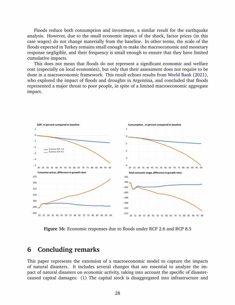
Floods reduce both consumption and investment, a similar result for the earthquakeanalysis. However, due to the small economic impact of the shock, factor prices (in thiscase wages) do not change materially from the baseline. In other terms, the scale of thefloods expected in Turkey remains small enough to make the macroeconomic and monetaryresponse negligible, and their frequency is small enough to ensure that they have limitedcumulative impacts.

This does not mean that floods do not represent a significant economic and welfarecost (especially on local economies), but only that their assessment does not require to bedone in a macroeconomic framework. This result echoes results from World Bank (2021),who explored the impact of floods and droughts in Argentina, and concluded that floodsrepresented a major threat to poor people, in spite of a limited macroeconomic aggregateimpact.

-.5

-.4

-.3

-.2

-.1

.0

.1

20 25 30 35 40 45 50 55 60 65 70 75 80 85 90 95 00

Scenario: RCP: 2.6Scenario: RCP: 8.5

GDP, in percent compared to baseline

-.4

-.3

-.2

-.1

.0

.1

20 25 30 35 40 45 50 55 60 65 70 75 80 85 90 95 00

Consumption , in percent compared to baseline

-.005

.000

.005

.010

.015

.020

.025

20 25 30 35 40 45 50 55 60 65 70 75 80 85 90 95 00

Consumer prices, difference in growth rates

-.012

-.010

-.008

-.006

-.004

-.002

.000

.002

20 25 30 35 40 45 50 55 60 65 70 75 80 85 90 95 00

Real consumer wage, difference in growth rates

Figure 16: Economic responses due to floods under RCP 2.6 and RCP 8.5

6 Concluding remarks

This paper represents the extension of a macroeconomic model to capture the impactsof natural disasters. It includes several changes that are essential to analyze the im-pact of natural disasters on economic activity, taking into account the specific of disaster-caused capital damages: (1) The capital stock is disaggregated into infrastructure and

28

non-infrastructure capital. (2) Private and public sector investment decisions into recon-struction are separated and explicitly modeled. (3) The impact of the shock on the produc-tivity of non-affected capital is explicitly introduced. (4) Realistic constraints on the paceof reconstruction are taken into account.

The marginal product of capital plays an important role in investment allocation de-cisions. The productivity of infrastructure capital increases significantly after a naturaldisaster, while the implications for non-infrastructure capital depend crucially on the elas-ticity of substitution between types of capital. Empirical estimates suggest that the twocapital stocks are complementary. Thus, if a natural disaster destroys infrastructure capi-tal, then non-infrastructure capital also becomes unproductive, which magnifies the impactof the disaster on GDP. In a simpler model where the capital stock is represented with aunique variable K, this effect would be equivalent to a loss in capital and a loss of totalfactor productivity (which is consistent with empirical observations).

In the model, large-scale disasters, exceeding the absorptive capacity of the economy,generate total (discounted) consumption losses that respond non-linearly to (and may ex-ceed) direct physical damage. This result is also consistent with empirical evidence. Forsmall disasters, the economic system can absorb the impact thanks to resource realloca-tion, imports, and borrowing, such that the total welfare cost is similar to or even lowerthan the direct physical damages.10 For larger disasters, the economy reaches the limits ofits ability to reallocate resources, the reconstruction period extends over several years, anddirect physical impacts are magnified. The absorptive capacity of the economy is controlledby a few parameters, including the ability of the economy to reallocate resources towardreconstruction and to implement the appropriate monetary policy response.

The destruction of capital (and the increase in the marginal product of capital) gen-erates inflation, which can be more or less persistent depending on price stickiness. Ifmonetary policy reacts immediately to the supply shock by increasing interest rates, eco-nomic effects are amplified. Monetary policy tightening increases the cost of borrowing forboth the government and the private sector and reduces consumption. A delayed response(usually when second round effects materialize due to changes in demand) can mitigatethe negative economic effects of disasters. However, in the context of climate change,increasingly frequent shocks may unanchor inflation expectations and reverse this result.

Fiscal policy adds another layer of complexity. The impact of disasters has both quantityand price responses. In our simulations, the short-run tax base response is dominated byprices, which lead to an increase in the nominal tax base and, in some of the simulations, atemporary reduction in nominal debt. This revenue gain is only temporary, as the medium-to long-term response to the disaster shock involves a reduction in the tax base. It isbeneficial, however, to invest in rebuilding the damaged capital, given that the returnon this investment is particularly high (because it increases the productivity of the non-infrastructure assets).

10This is ignoring the direct human impact of disasters, or assuming it can be avoided thanks to well-managed early warning systems and evacuation, or buildings designed not to collapse during an earthquake.

29

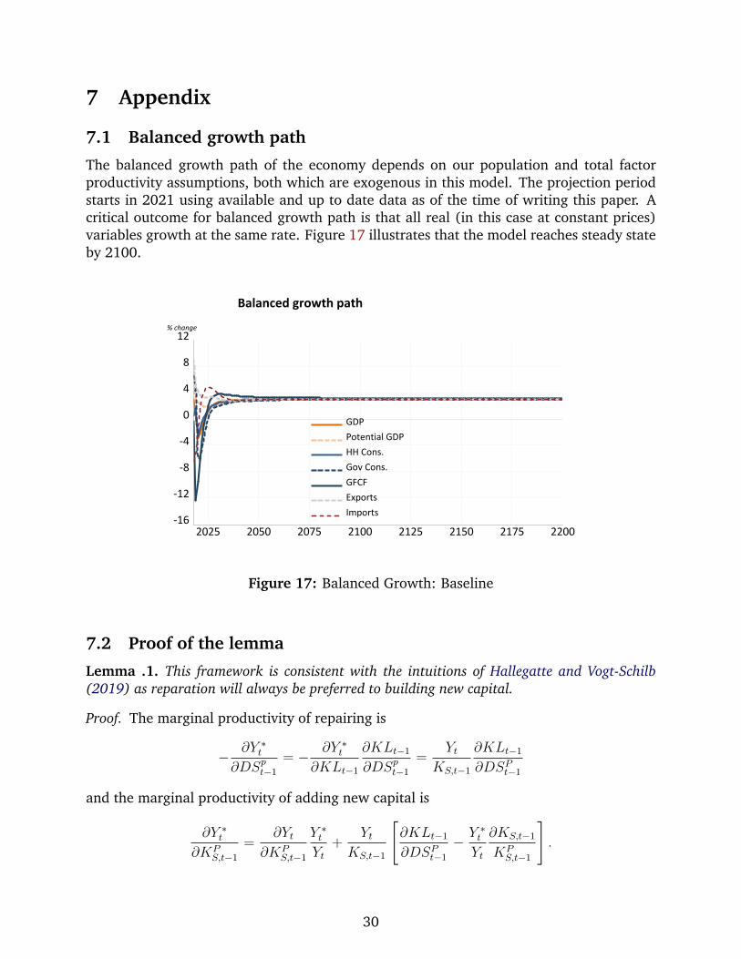
7 Appendix

7.1 Balanced growth path

The balanced growth path of the economy depends on our population and total factorproductivity assumptions, both which are exogenous in this model. The projection periodstarts in 2021 using available and up to date data as of the time of writing this paper. Acritical outcome for balanced growth path is that all real (in this case at constant prices)variables growth at the same rate. Figure 17 illustrates that the model reaches steady stateby 2100.

-16

-12

-8

-4

0

4

8

12

2025 2050 2075 2100 2125 2150 2175 2200

GDPPotential GDPHH Cons.Gov Cons.GFCFExportsImports

Balanced growth path% change

Figure 17: Balanced Growth: Baseline

7.2 Proof of the lemma

Lemma .1. This framework is consistent with the intuitions of Hallegatte and Vogt-Schilb(2019) as reparation will always be preferred to building new capital.

Proof. The marginal productivity of repairing is

− ∂Y ∗t

∂DSpt−1

= − ∂Y ∗t

∂KLt−1

∂KLt−1

∂DSpt−1

=Yt

KS,t−1

∂KLt−1

∂DSPt−1

and the marginal productivity of adding new capital is

∂Y ∗t

∂KPS,t−1

=∂Yt

∂KPS,t−1

Y ∗t

Yt

+Yt

KS,t−1

[∂KLt−1

∂DSPt−1

− Y ∗t

Yt

∂KS,t−1

KPS,t−1

].

30

One can note that

∂Y ∗t

∂KPS,t−1

= − ∂Y ∗t

∂DSpt−1

+Y ∗t

Yt

[∂Yt

∂KPS,t−1

− ∂KS,t−1

KPS,t−1

]

where

[∂Yt

∂KPS,t−1

− ∂KS,t−1

KPS,t−1

]=

∂KS,t−1

∂KPS,t−1︸ ︷︷ ︸>0

∂Yt

∂KS,t−1︸ ︷︷ ︸<1 because of decreasing return of the Cobb-Douglas in K

−1

︸ ︷︷ ︸

<0

Hence,∂Y ∗

t

∂KPS,t−1

< − ∂Y ∗t

∂DSpt−1

.

In words, the marginal productivity of repairing is always higher than the marginal pro-ductivity of adding new capital stocks.

References

Aiyagari, S. R. (1994). Uninsured idiosyncratic risk and aggregate saving. The QuarterlyJournal of Economics, 109(3):659–684.

Akao, K.-I. and Sakamoto, H. (2018). A theory of disasters and long-run growth. Journalof Economic Dynamics and Control, 95(C):89–109.

An, Z., Kangur, A., and Papageorgiou, C. (2019). On the substitution of private and publiccapital in production. European Economic Review, 118:296–311.

Bakkensen, L. and Barrage, L. (2021). Climate shocks, cyclones, and economic growth:Bridging the micro-macro gap. NBER Working Paper w24893, National Bureau of Eco-nomic Research.

Baqaee, D. and Farhi, E. (2020). Nonlinear production networks with an application to thecovid-19 crisis. Technical report, National Bureau of Economic Research.

Barrot, J.-N. and Sauvagnat, J. (2016). Input specificity and the propagation of idiosyn-cratic shocks in production networks. The Quarterly Journal of Economics, 131(3):1543–1592.

Batten, S., Sowerbutts, R., and Tanaka, M. (2016). Let’s talk about the weather: the impactof climate change on central banks.

Bewley, T. (1977). The permanent income hypothesis: A theoretical formulation. Journalof Economic Theory, 16(2):252–292.

31

Boehm, C. E., Flaaen, A., and Pandalai-Nayar, N. (2019). Input Linkages and the Transmis-sion of Shocks: Firm-Level Evidence from the 2011 Tohoku Earthquake. The Review ofEconomics and Statistics, 101(1):60–75.

Burke, M., Hsiang, S. M., and Miguel, E. (2015). Global non-linear effect of temperatureon economic production. Nature, 527(7577):235–239.

Burns, A., Campagne, B., Jooste, C., Stephan, D., and Bui, T. T. (2019). The worldbank macro-fiscal model technical description. Policy Research Working Paper 8965,The World Bank, Washington, DC.

Burns, A. and Jooste, C. (2019). Estimating and calibrating mfmod : A panel data approachto identifying the parameters of data poor countries in the world bank’s structural macromodel. Policy Research Working Paper 8939, The World Bank, Washington, DC.

Burns, A., Jooste, C., and Schwerhoff, G. (2020). Macroeconomic modeling of managinghurricane damage in the caribbean: The case of jamaica. Policy Research Working Paper9505, The World Bank, Washington, DC.

Camacho, C. and Sun, Y. (2017). Longterm decision making under the threat of earth-quakes. PSE Working Papers halshs-01670507, HAL.

Cavallo, A., Cavallo, E., and Rigobon, R. (2014). Prices and supply disruptions duringnatural disasters. Review of Income and Wealth, 60:S449–S471.

Colon, C., Hallegatte, S., and Rozenberg, J. (2021). Criticality analysis of a country’s trans-port network via an agent-based supply chain model. Nature Sustainability, 4(3):209–215.

Dell, M., Jones, B. F., and Olken, B. A. (2012). Temperature shocks and economicgrowth: Evidence from the last half century. American Economic Journal: Macroeco-nomics, 4(3):66–95.

Dieppe, A., Kilic Celik, S., and Okou, C. (2020). Implications of major adverse events onproductivity. Working Paper 9411, The World Bank.

Dietz, S. and Stern, N. (2015). Endogenous growth, convexity of damage and climaterisk: how nordhaus’ framework supports deep cuts in carbon emissions. The EconomicJournal, 125(583):574–620.

Doyle, L. and Noy, I. (2015). The short-run nationwide macroeconomic effects of thecanterbury earthquakes. New Zealand Economic Papers, 49(2):134–156.

Ehrmann, M. and Smets, F. (2003). Uncertain potential output: implications for monetarypolicy. Journal of Economic Dynamics and Control, 27(9):1611–1638.

Elliott, J., Muller, C., Deryng, D., Chryssanthacopoulos, J., Boote, K. J., Buchner, M., Fos-ter, I., Glotter, M., Heinke, J., Iizumi, T., Izaurralde, R. C., Mueller, N. D., Ray, D. K.,Rosenzweig, C., Ruane, A. C., and Sheffield, J. (2015). The global gridded crop modelintercomparison: Data and modeling protocols for phase 1 (v1.0). Geosci. Model Dev.,8:261–277.

32

Fankhauser, S. and Tol, R. S. (2005). On climate change and economic growth. Resourceand Energy Economics, 27(1):1–17.

Feenstra, R. C., Inklaar, R., and Timmer, M. P. (2015). The next generation of the pennworld table. American Economic Review, 105(10):3150–3182.

Felbermayr, G. and Groschl, J. (2014). Naturally negative: The growth effects of naturaldisasters. Journal of Development Economics, 111(C):92–106.

Ferrero, G., Pietrunti, M., and Tiseno, A. (2019). Benefits of gradualism or costs of inaction?monetary policy in times of uncertainty. Monetary Policy in Times of Uncertainty (February4, 2019). Bank of Italy Temi di Discussione (Working Paper) No, 1205.

Ginn, W. (2021). Climate disasters and the macroeconomy: Does state-dependence mat-ter? evidence for the us. EconDisCliCha.

Hallegatte, S. and Ghil, M. (2008). Natural disasters impacting a macroeconomic modelwith endogenous dynamics. Ecological Economics, 68(1):582–592.

Hallegatte, S., Ghil, M., Dumas, P., and Hourcade, J.-C. (2008). Business cycles, bifurca-tions and chaos in a neo-classical model with investment dynamics. Journal of EconomicBehavior & Organization, 67(1):57–77.

Hallegatte, S., Hourcade, J.-C., and Dumas, P. (2007). Why economic dynamics matter inassessing climate change damages: Illustration on extreme events. Ecological Economics,62(2):330–340.

Hallegatte, S. and Vogt-Schilb, A. (2019). Are losses from natural disasters more than justasset losses? In Advances in Spatial and Economic Modeling of Disaster Impacts, pages15–42. Springer.

Hallegatte, S., Vogt-Schilb, A., Bangalore, M., and Rozenberg, J. (2017). Unbreakable :Building the Resilience of the Poor in the Face of Natural Disasters. Washington, dc:World bank, World Bank.

Henriet, F., Hallegatte, S., and Tabourier, L. (2012). Firm-network characteristics andeconomic robustness to natural disasters. 36(1):150–167.

Howell, W., Evans, P., Devereux, S., Sage, D., Smith, J., and Haegert, D. (1993). Absence ofstrong hla-dr/dq-dp linkage disequilibrium in the british and french canadian caucasoidpopulations. International Journal of Immunogenetics, 20(5):363–371.

Hsiang, S. M. and Jina, A. S. (2014). The causal effect of environmental catastropheon long-run economic growth: Evidence from 6,700 cyclones. Working Paper 20352,National Bureau of Economic Research.

Ikefuji, M. and Horii, R. (2012). Natural disasters in a two-sector model of endogenousgrowth. Journal of Public Economics, 96(9-10):784–796.

Inoue, H. and Todo, Y. (2019). Firm-level propagation of shocks through supply-chainnetworks. Nature Sustainability, 2(9):841–847.

33

IPCC (2012). Managing the risks of extreme events and disasters to advance climate changeadaptation. a special report of working groups i and ii of the intergovernmental panelon climate change [field, c.b., v. barros, t.f. stocker, d. qin, d.j. dokken, k.l. ebi, m.d.mastrandrea, k.j. mach, g.-k. plattner, s.k. allen, m. tignor, and p.m. midgley (eds.)].Technical report, IPCC, United Kingdom and New York, NY, USA.

Isore, M. and Szczerbowicz, U. (2017). Disaster risk preference shifts in a new keyenesianmodel. Journal of Economic Dynamics and Control, 79:97–125.

Klomp, J. (2020). Do natural disasters affect monetary policy? a quasi-experiment ofearthquakes. Journal of Macroeconomics, 64:103164.

Krebs, T. (2003a). Growth and Welfare Effects of Business Cycles in Economies with Id-iosyncratic Human Capital Risk. Review of Economic Dynamics, 6(4):846–868.

Krebs, T. (2003b). Human capital risk and economic growth. The Quarterly Journal ofEconomics, 118(2):709–744.

Lackner, S. (2018). Earthquakes and economic growth. FIW Working Paper 190, FIW -Research Centre International Economics.

Marto, R., Papageorgiou, C., and Klyuev, V. (2018). Building resilience to natural disasters:An application to small developing states. Journal of Development Economics, 135:574–586.

Moore, F. C. and Diaz, D. B. (2015). Temperature impacts on economic growth warrantstringent mitigation policy. Nature Climate Change, 5(2):127–131.

Myhre, G., Alterskjær, K., Stjern, C., Hodnebrog, , Marelle, L., Samset, B., Sillmann, J.,Schaller, N., Fischer, E., Schulz, M., and Stohl, A. (2019). Frequency of extreme precipi-tation increases extensively with event rareness under global warming. Scientific Reports,16063.

Muller-Furstenberger, G. and Schumacher, I. (2015). Insurance and climate-driven extremeevents. Journal of Economic Dynamics and Control, 54(C):59–73.

Nordhaus, W. D. (1992). An optimal transition path for slowing climate change. Science,20:1315–1319.

Nordhaus, W. D. and Moffat, A. (2017). A Survey of Global Impacts of Climate Change:Replication, Survey Methods, and a Statistical Analysis. NBER Working Papers 23646,National Bureau of Economic Research, Inc.

Ocal, A. (2019). Natural disasters in turkey: Social and economic perspective. InternationalJournal of Disaster Risk Management, 1(1):51–61.

Parker, M. (2018). The impact of disasters on inflation. Economics of Disasters and ClimateChange, 2(1):21–48.

Raddatz, C. (2007). Are external shocks responsible for the instability of output in low-income countries? Journal of Development Economics, 84(1):155–187.

34

Rao, A., Calderon, A., Silva, V., Martins, L., and Paul, N. (2022). Earthquake risk assess-ment and retrofit scenarios for turkey, exposure model development probabilistic seismicrisk analysis retrofit intervention scenarios. Technical report, Global Earthquake Model.

Rose, A. and Liao, S.-Y. (2005). Modeling regional economic resilience to disasters: Acomputable general equilibrium analysis of water service disruptions. Journal of RegionalScience, 45(1):75–112.

Rose, A. and Wei, D. (2013). Estimating the economic consequences of a port shutdown:the special role of resilience. Economic Systems Research, 25(2):212–232.

Rudebusch, G. D. et al. (2019). Climate change and the federal reserve. FRBSF EconomicLetter, 9.

Strobl, E. (2011). The economic growth impact of hurricanes: Evidence from u.s. coastalcounties. The Review of Economics and Statistics, 93(2):575–589.

UNISDR (2015). Global assessment report on disaster risk reduction. Last accessed 18December 2021.

Wood, A., Noy, I., and Parker, M. (2016). The canterbury rebuild five years on from thechristchurch earthquake. Bulletin 3, Reserve Bank of New Zealand.

World Bank (1999). Turkey marmara earthquake assessment. Report 27380, Turkey Coun-try Office.

World Bank (2021). Poverty and macro economic impacts of climate shocks. Technicalreport, The World Bank.

Wright, A. and Borda, P. (2016). Macroeconomic fluctuations under natural disaster shocksin central america and the caribbean. IDB Working Paper Series 463, IDB.

35