Research Series No. 62 Macroeconomic and Welfare Consequences of High Energy Prices Evarist Twimukye and John Mary Matovu May, 2009 Economic Policy Research Centre (EPRC) 51 Pool Road Makerere University Campus, P. O. Box 7841 Kampala, Uganda Tel: 256-41-541023, Fax: 256-41-541022, Email: [email protected]

Welcome message from author
This document is posted to help you gain knowledge. Please leave a comment to let me know what you think about it! Share it to your friends and learn new things together.
Transcript
Research Series No. 62
Macroeconomic and Welfare Consequences of
High Energy Prices
Evarist Twimukye and John Mary Matovu
May, 2009
Economic Policy Research Centre (EPRC) 51 Pool Road Makerere University Campus, P. O. Box 7841 Kampala, Uganda Tel: 256-41-541023, Fax: 256-41-541022, Email: [email protected]

See the end of this document for a list of previous papers in the series
Macroeconomic and Welfare Consequences of High Energy Prices
Evarist Twimukye and John Mary Matovu
May, 2009
i
Abstract The current wave of volatile international oil prices coupled with the low hydro-
energy generation continues to exert negative impacts on the Ugandan
economy. This paper analyses the extent to which changes in energy prices
affect the economy and examines policy options that can be undertaken to
circumvent the negative effects. The impact of higher oil prices takes a large toll
on all sectors including agriculture, manufacturing and services. With the existing
losses in productivity of generating hydro electricity, this has exacerbated the
energy crisis. The combined output loss for the manufacturing sector due to
increase in fuel prices and a shortage of electricity is estimated at 2 per cent on
annual basis. While the government has little control on the international prices of
oil, further private and public investments in the energy sector are called for to
alleviate the shortages of energy.
1
A. Introduction
The impact of oil shocks on national economies has been of concern to many
countries, as a constraint to economic development. Recently, international oil
prices have risen sharply and reached record levels, and coupled with Uganda’s
reliance on oil imports, this has had an adverse impact on the country’s
economy. Although this is not limited to Uganda, the country’s location and the
recent natural and regional problems make it even more vulnerable to oil shocks.
Uganda has neither crude oil production nor a refinery and is entirely dependent
on imports of petroleum products, although it has recently discovered some oil
reserves in the western region of the country. With recent power shortages in the
country (resulting from reduced electricity generation from the only two power
stations), and a hike in global oil prices, there has been an increase in the oil
imports especially diesel for thermal power generation. According to government
statistics, Uganda consumed about 792,555m3 of petroleum products in 2006. Of
the total, 28.5 per cent by volume was diesel, 25 per cent gasoline, 11.4 per cent
aviation fuel, 5.4 per cent kerosene, and 1 per cent LPG (UBOS, 2007; Figure 1).
The increase in oil prices and reduced generation of electricity has had both
direct and indirect effects on the economy. First, the reduction in electricity
generation has significantly affected the manufacturing sector. This is due to the
unexpected power outages and load shedding. In some cases companies have
resorted to use of generators, albeit the increasing international prices of oil. This
has resulted into lost output and in some instances bankruptcies. Increasing fuel
prices have weighed heavily on the transportation sector while at the same time
increasing the cost of generating thermal power.
Given that there are short and long-term implications of volatile fuel prices, we
use a dynamic general equilibrium model to capture the effects especially at a
sectoral level. For oil prices, we first assume that the increase is permanent, a
2
phenomenon which reflects what is on the ground in Uganda. The second
simulation assumes that the oil prices revert back to their original levels in line
with the international crude oil prices. The third simulation focuses on the marked
reduction in electricity generated owing to the inefficiencies in the sector and the
natural causes like the reduction of the water level of Lake Victoria. The fourth
simulation assumes that the inefficiency in the utility sector is temporary and
addressed by attracting private investments. Lastly, we explore the case where
the government reduces tariffs on oil imports to circumvent the price increase.
The key results suggest that the changes in oil prices have sizable negative
effects especially at the sectoral level. While at the aggregate level, GDP might
not be affected as more activity is realised in the trading sector, increase in oil
prices would significantly reduce the output for agriculture, manufacturing and
transports. The reduction in output for these sectors is subdued when the oil
price shock is temporary. On the other hand, the low efficiency in the electricity
sector has also negatively affected the sectors. The combined effects of oil price
shocks and reduction in electricity generated would reduce overall growth rate of
the manufacturing sector by 2 per centage points on annual basis.
This paper has some policy implications. First, at a time of high oil prices, the
government can intervene by lowering tariffs on oil products. However, this has
to take into account the trade-off between the oil tariff revenues and taxes lost
owing to reduced economic activity especially in the manufacturing sector.
Second, the government should take a more active role on suppliers where
prices should be adjusted downwards when international prices drop. As found,
the output losses are much higher when the price increase remains permanent.
Third, without addressing the inefficiencies in the electricity sector, this will
continue to affect the output of manufacturing and other sectors that depend on
electricity. More private-public investments should be encouraged to enhance the
productivity of the sector.
3
B. Background B.1 Volatility of World Crude Oil Prices On average, the international spot prices of crude oil jumped from an annual
average of $12 per barrel in 1998 to $94 in 2008, a phenomenal 780% increase
in just 10 years (Energy Information Administration (EIA), 2008). Among factors
that contributed to the hike was an unabated strong demand in the emerging
economies and continuous tension in Middle-East region, the largest oil
supplying region. Speculations on oil prices in future markets also played an
important part in the price hikes, even though the supply seems to increase
proportionally to meet demand in the last few years. Recently, the prices have
been on a downward trend owing to the ongoing recession in the US and other
developed countries. Various studies have suggested that any US$10 increase in
oil price per barrel would cause about 1 per cent reduction in the world’s gross
national product (GDP) and a 0.6 per cent increase in the world price.
As far as Uganda is concerned, the component of retail prices of oil was
demystified and its one-off affects on the economy can be explored. The spiral of
higher oil prices has driven retail prices to record highs. The Government has
made it clear to the market and consumers that there is nothing it can do to
respond to the oil shocks. The entire dependence of the country on oil imports
and inability to substitute consumption of oil products are also factors for
suppliers to exhort higher prices on consumers. Moreover, it is very likely that the
lack of fair competition has allowed all oil companies to collude to set higher
prices simultaneously in order to keep their profit margins as high as possible.
Indeed even as world prices of crude oil continue to fall, suppliers have
maintained the old prices when the barrel of oil was trading at US$ 150 dollars.
Evidently, the retail prices of gasoline and diesel have reached 2,563 and 2,350
Uganda Shillings per litre, respectively for the first quarter of 2008 compared with
1,763 and 1,513 per litre in 2004, nearly 50 per cent higher and there are no
4
signs of the prices dropping even when the crude prices have plummeted to a
third of their record levels. Even though the impacts of this hike seem to be
evident, the Government has yet to genuinely look for alternative policies. The
justification of the Government’s “laissez-fair” approach is the pronounced impact
on tax revenue reduction, should it lower tariffs and taxes imposed on oil imports
and consumption. Tax revenue from oil was about 535 Billion Uganda Shillings in
2007, accounting for more than 19 per cent of total tax revenue.
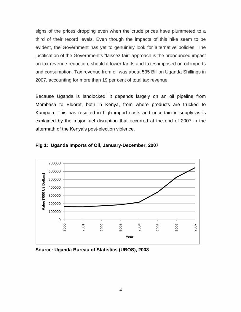
Because Uganda is landlocked, it depends largely on an oil pipeline from
Mombasa to Eldoret, both in Kenya, from where products are trucked to
Kampala. This has resulted in high import costs and uncertain in supply as is
explained by the major fuel disruption that occurred at the end of 2007 in the
aftermath of the Kenya’s post-election violence.
Fig 1: Uganda Imports of Oil, January-December, 2007
Source: Uganda Bureau of Statistics (UBOS), 2008
0
100000
200000
300000
400000
500000
600000
700000
2000
2001
2002
2003
2004
2005
2006
2007
Value
('00
0 US Dollars)
Year
5
B.2 The Oil Industry in Uganda Uganda’s downstream oil sector was liberalized in 1994, and price controls and
bureaucratic resource allocation were abolished and a new petroleum supply act
was promulgated in October 2003. This led to the licensing of several
companies, including several international oil companies like Shell, Total, and
Caltex to take part in the industry. Although the sector is fairly competitive with
even smaller firms operating, the market is dominated by the few international
ones the top three being Shell, Total and Caltex (Ministry of Mineral and Energy
Development 2008). The persistently high prices of petroleum products in spite
of the falls in the world crude prices have raised alarms in the population that the
industry may be poorly regulated, making players to collude to cheat the
motorists.
B.3 Energy Price Movements in Uganda1 Uganda’s fuel woes are closely linked to the recent power shortages that have
increased the need for supplementary power to support the dwindling
Hydroelectric Power (HEP) from the two dams in the country. The recent
prolonged drought in East Africa and the derelict power grid has caused a
serious shortage of electricity, and this pressure on the power system prompted
the government to encourage the entry of private firms to generate power from
diesel operated thermal generators and supply it to the national grid.
But in spite of this, power supply has lagged the power needs of the country
resulting in a load-shedding program introduced in February 2006, that has often
involved cutting power off for more than 12 hours every day to all consumers
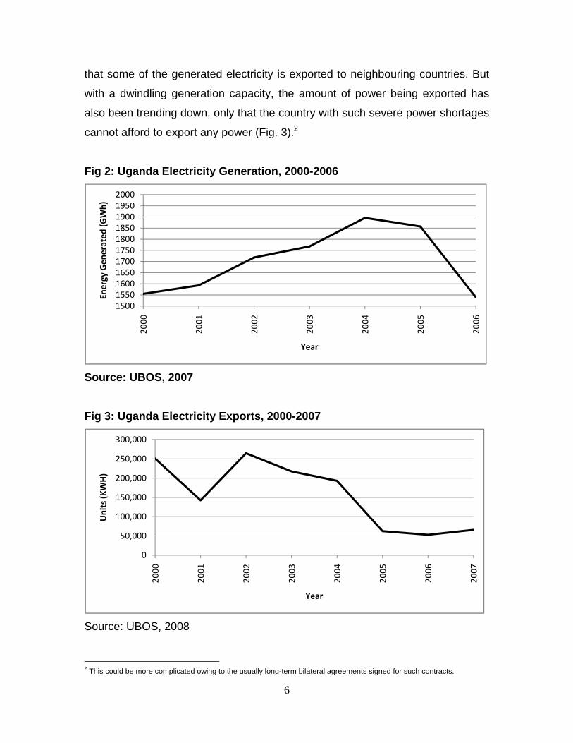
except certain key installations (such as hospitals). As of the end of 2006 the
hydroelectric dams with an installed capacity of 356 MW were operating at less
than one-half of the capacity, with the power generated being supplemented by a
100 MW diesel-fired generators (Fig.2). This shortage is aggravated by the fact
1 Energy here refers to a combination of fuel for automobiles, manufacturing, etc and electricity
6
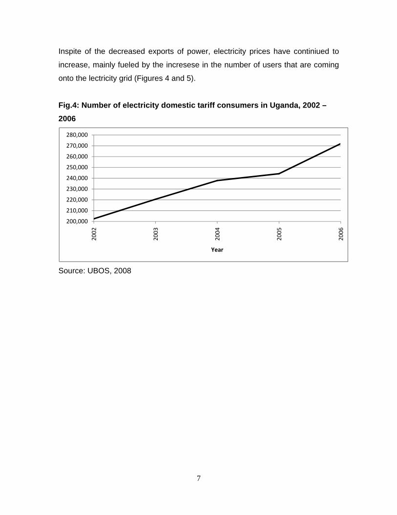
that some of the generated electricity is exported to neighbouring countries. But
with a dwindling generation capacity, the amount of power being exported has
also been trending down, only that the country with such severe power shortages
cannot afford to export any power (Fig. 3).2
Fig 2: Uganda Electricity Generation, 2000-2006
Source: UBOS, 2007 Fig 3: Uganda Electricity Exports, 2000-2007
Source: UBOS, 2008
2 This could be more complicated owing to the usually long-term bilateral agreements signed for such contracts.
15001550160016501700175018001850190019502000
2000
2001
2002
2003
2004
2005
2006
Energy Gen
erated
(GWh)
Year
0
50,000
100,000
150,000
200,000
250,000
300,000
2000
2001
2002
2003
2004
2005
2006
2007
Units (K
WH)
Year
7
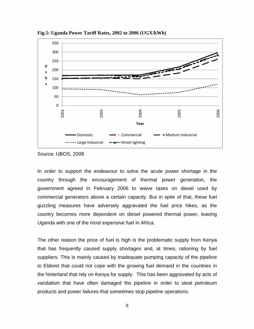
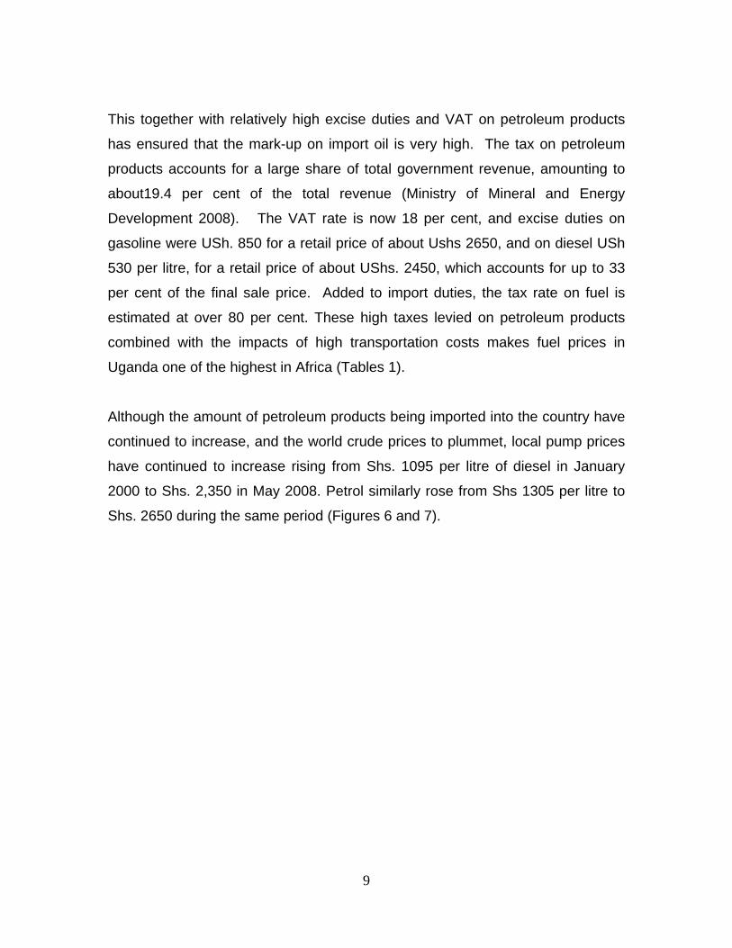
Inspite of the decreased exports of power, electricity prices have continiued to
increase, mainly fueled by the incresese in the number of users that are coming
onto the lectricity grid (Figures 4 and 5).
Fig.4: Number of electricity domestic tariff consumers in Uganda, 2002 – 2006
Source: UBOS, 2008
200,000
210,000
220,000
230,000
240,000
250,000
260,000
270,000
280,000
2002
2003
2004
2005
2006
Year
8
Fig.5: Uganda Power Tariff Rates, 2002 to 2006 (UGX/kWh)
Source: UBOS, 2008
In order to support the endeavour to solve the acute power shortage in the
country through the encouragement of thermal power generation, the
government agreed in February 2006 to waive taxes on diesel used by
commercial generators above a certain capacity. But in spite of that, these fuel
guzzling measures have adversely aggravated the fuel price hikes, as the
country becomes more dependent on diesel powered thermal power, leaving
Uganda with one of the most expensive fuel in Africa.
The other reason the price of fuel is high is the problematic supply from Kenya
that has frequently caused supply shortages and, at times, rationing by fuel
suppliers. This is mainly caused by inadequate pumping capacity of the pipeline
to Eldoret that could not cope with the growing fuel demand in the countries in
the hinterland that rely on Kenya for supply. This has been aggravated by acts of
vandalism that have often damaged the pipeline in order to steal petroleum
products and power failures that sometimes stop pipeline operations.
0
50
100
150
200
250
300
350
2002
2003
2004
2005
2006
Ushs
Year
Domestic Commercial Medium Industrial
Large Industrial Street lighting
9
This together with relatively high excise duties and VAT on petroleum products
has ensured that the mark-up on import oil is very high. The tax on petroleum
products accounts for a large share of total government revenue, amounting to
about19.4 per cent of the total revenue (Ministry of Mineral and Energy
Development 2008). The VAT rate is now 18 per cent, and excise duties on
gasoline were USh. 850 for a retail price of about Ushs 2650, and on diesel USh
530 per litre, for a retail price of about UShs. 2450, which accounts for up to 33
per cent of the final sale price. Added to import duties, the tax rate on fuel is
estimated at over 80 per cent. These high taxes levied on petroleum products
combined with the impacts of high transportation costs makes fuel prices in
Uganda one of the highest in Africa (Tables 1).
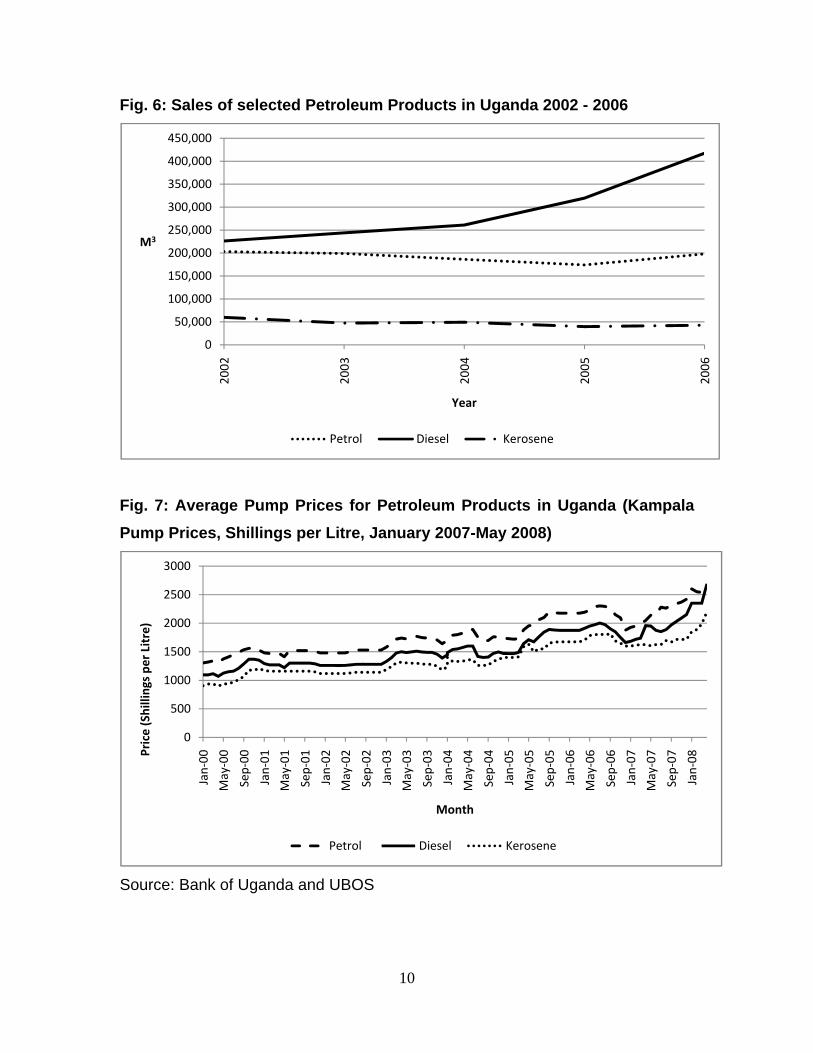
Although the amount of petroleum products being imported into the country have
continued to increase, and the world crude prices to plummet, local pump prices
have continued to increase rising from Shs. 1095 per litre of diesel in January
2000 to Shs. 2,350 in May 2008. Petrol similarly rose from Shs 1305 per litre to
Shs. 2650 during the same period (Figures 6 and 7).
10
Fig. 6: Sales of selected Petroleum Products in Uganda 2002 - 2006
Fig. 7: Average Pump Prices for Petroleum Products in Uganda (Kampala Pump Prices, Shillings per Litre, January 2007-May 2008)
Source: Bank of Uganda and UBOS
0
50,000
100,000
150,000
200,000
250,000
300,000
350,000
400,000
450,000
2002
2003
2004
2005
2006
M3
Year
Petrol Diesel Kerosene
0
500
1000
1500
2000
2500
3000
Jan‐00
May‐00
Sep‐00
Jan‐01
May‐01
Sep‐01
Jan‐02
May‐02
Sep‐02
Jan‐03
May‐03
Sep‐03
Jan‐04
May‐04
Sep‐04
Jan‐05
May‐05
Sep‐05
Jan‐06
May‐06
Sep‐06
Jan‐07
May‐07
Sep‐07
Jan‐08Pr
ice (Shillings pe
r Litre)
Month
Petrol Diesel Kerosene
11
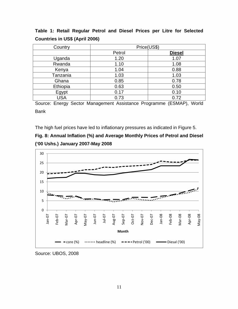
Table 1: Retail Regular Petrol and Diesel Prices per Litre for Selected Countries in US$ (April 2006)
Country Price(US$) Petrol Diesel
Uganda 1.20 1.07 Rwanda 1.10 1.08 Kenya 1.04 0.88
Tanzania 1.03 1.03 Ghana 0.85 0.78
Ethiopia 0.63 0.50 Egypt 0.17 0.10 USA 0.73 0.72
Source: Energy Sector Management Assistance Programme (ESMAP), World
Bank
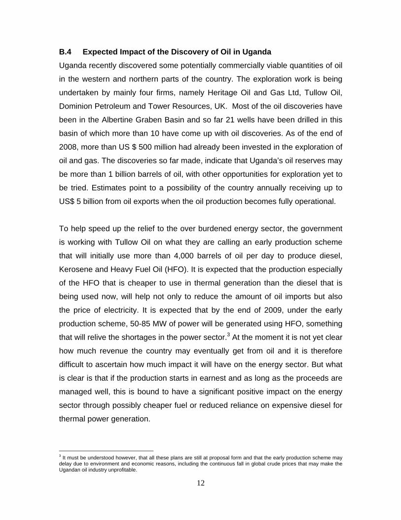
The high fuel prices have led to inflationary pressures as indicated in Figure 5. Fig. 8: Annual Inflation (%) and Average Monthly Prices of Petrol and Diesel (‘00 Ushs.) January 2007-May 2008
Source: UBOS, 2008
0
5
10
15
20
25
30
Jan‐07
Feb‐07
Mar‐07
Apr‐07
May‐07
Jun‐07
Jul‐0
7
Aug
‐07
Sep‐07
Oct‐07
Nov‐07
Dec‐07
Jan‐08
Feb‐08
Mar‐08
Apr‐08
May‐08
Month
core (%) headline (%) Petrol ('00) Diesal ('00)
12
B.4 Expected Impact of the Discovery of Oil in Uganda Uganda recently discovered some potentially commercially viable quantities of oil
in the western and northern parts of the country. The exploration work is being
undertaken by mainly four firms, namely Heritage Oil and Gas Ltd, Tullow Oil,
Dominion Petroleum and Tower Resources, UK. Most of the oil discoveries have
been in the Albertine Graben Basin and so far 21 wells have been drilled in this
basin of which more than 10 have come up with oil discoveries. As of the end of
2008, more than US $ 500 million had already been invested in the exploration of
oil and gas. The discoveries so far made, indicate that Uganda’s oil reserves may
be more than 1 billion barrels of oil, with other opportunities for exploration yet to
be tried. Estimates point to a possibility of the country annually receiving up to
US$ 5 billion from oil exports when the oil production becomes fully operational.
To help speed up the relief to the over burdened energy sector, the government
is working with Tullow Oil on what they are calling an early production scheme
that will initially use more than 4,000 barrels of oil per day to produce diesel,
Kerosene and Heavy Fuel Oil (HFO). It is expected that the production especially
of the HFO that is cheaper to use in thermal generation than the diesel that is
being used now, will help not only to reduce the amount of oil imports but also
the price of electricity. It is expected that by the end of 2009, under the early
production scheme, 50-85 MW of power will be generated using HFO, something
that will relive the shortages in the power sector.3 At the moment it is not yet clear
how much revenue the country may eventually get from oil and it is therefore
difficult to ascertain how much impact it will have on the energy sector. But what
is clear is that if the production starts in earnest and as long as the proceeds are
managed well, this is bound to have a significant positive impact on the energy
sector through possibly cheaper fuel or reduced reliance on expensive diesel for
thermal power generation.
3 It must be understood however, that all these plans are still at proposal form and that the early production scheme may delay due to environment and economic reasons, including the continuous fall in global crude prices that may make the Ugandan oil industry unprofitable.
13
C. Objectives of the Study The main objective of the study is to assess the impact of the high energy prices
and reduced electricity generation on the Uganda economy especially on the
manufacturing sector. The study seeks to investigate how the recent increases in
the prices of energy and the low generation of electricity have affected the overall
macro-economy, different sectors of the economy and the welfare of different
sections of the population.
D. Justification of the Study Whereas it is taken for granted that high energy prices have a detrimental impact
on economies of oil importing countries like Uganda, there is a paucity of studies
that have gone ahead to empirically prove this for Uganda. One of the reasons
for this is because high energy prices have only recently become a global threat
to economic growth. This has necessitated that the impact of these oil shocks be
investigated to provide policy makers with evidence of efficacy of the energy
policies that they are undertaking and how they affect both the economy and the
welfare of the population. Although the Energy Sector Management Assistance
Programme (ESMAP) of the World Bank has routinely been assessing the impact
of energy prices on the world economies, it has been using only descriptive
assessment without rigorous empirical assessment (See for Example, Bacon and
Kojima, 2006; Bacon, R., and Mattar, A., 2005). Moreover, we do not know of
any study that has empirically studied the impact of an increase in the price of
both petroleum and electric power in Uganda. Based on an economy-wide
extensive SAM which was recently released by the Uganda National Bureau of
Statistics (UBOS), based on 2007 data, our CGE analysis empirically assesses
the macroeconomic and welfare impacts of high energy prices in Uganda.
14
E. Literature Review The impact of the high energy prices on the economy both at the macro and
micro level is well documented in many studies. Not only does it affect the firms’
activities but it also generally impact negatively on the whole economy. Lee and
Ni, 2002 found that for industries that have a large cost share of oil, such as
petroleum refinery and industrial chemicals, oil price shocks mainly reduce
supply but for other industries, with the automobile industry being a particularly
important example, oil price shocks mainly reduce demand, suggesting that oil
price shocks influence economic activities beyond that explained by direct input
cost effects, possibly by delaying purchasing decisions of durable goods.
Schneider, 2004 also found that oil price shocks affect the economy through the
supply side (higher production costs, reallocation of resources), the demand side
(income effects, uncertainties) and the terms of trade. The paper also found that
an increase in the price of oil feeds through to GDP growth to a much larger
extent than a decline, a phenomenon that can be attributed to adjustment costs
associated with sectoral reallocations, the implications of uncertainties for
spending on consumer durables and investment, and nominal wage rigidities.
Furthermore, the element of surprise in oil price hikes seems to play a
considerable role. Thus, the paper continues, when a rise in the price of oil
occurs after a prolonged period of oil price stability, it has a larger impact than a
price hike which immediately follows previous cuts.
To emphasize the importance of oil in the economic health of even developed
countries, Carlstrom and Fuerst, 2005 contend that every U.S. recession since
1971 has been preceded by two things: an oil price shock and an increase in the
federal funds rate.
Abeysinghe, 2001 measuring the direct and indirect effects of oil prices on GDP
growth of 12 economies, finds that that the transmission effect of oil prices on
growth may not be that important for a large economy like the US but it could
15
play a critical role in small open economies with the biggest impact being the
effect of the shock and its interaction with consumer and investor confidence.
Using a GEM-E3 world model to carry out a comparative statics analysis of the
potential impact of oil price rises on the EU economy, Ciscar., et. al, 2004, found
out that crude petroleum, petroleum refineries and energy-intensive sectors
undergo a significant fall in their value-added with almost 40 per cent of the
overall GDP fall coming from other service sector, while the trade and transport
sector and the other equipment goods sector represent each approximately 10
per cent of the overall GDP fall. They found that the GDP losses for the EU as a
whole were 0.94 per cent in a scenario where oil was increased by $10 and 2.56
per cent in the second where the oil was increased by $30. Whereas they found
that the macroeconomic impact is slightly lower in the USA (0.81 per cent and
2.21 per cent, respectively), Australia, the FSU, India and Japan had similar
losses to that of the whole EU, while China and Africa experienced a bigger GDP
drop. Taking the African case it seems to suggest that the pass-through effects of
increased oil prices is particularly more harmful to African countries like Uganda.
Pradhan, and Sahoo, 2000, using CGE to analyse the impact of international oil
price shock on the Indian economy found that it affects the welfare and poverty of
households directly as well as indirectly. The paper found that oil shock leads to
decline in household welfare and increase in poverty and that with the increase in
elasticity of substitution of demand for imports to domestically produced crude oil,
welfare loss for household groups goes on increasing. The paper found that the rise
in rural poverty is concentrated among non-agricultural labour and other household
groups, while that for urban area is reflected in non-agricultural household group.
Other researchers who have used CGE to study the impact on the economy of high
oil prices are Adenikinju and Falobi, 2006 who find that the oil sector supply
shocks in Nigeria are costly both directly and indirectly resulting in lower real
GDP, higher average prices and greater balance of payment deficits. They also
16
find that other macroeconomic variables such as private consumption,
investment, government revenue and employment also decline. In addition, they
find that the distributional impact of the quantitative energy supply shocks is
higher for poor households than rich households.
Nkomo, 2006 contend that in Southern African countries, energy shocks affect
the economies because energy consumers and producers are constrained by
their energy consuming appliances which are fixed in the short-run, thus making
it difficult to shift to less oil intensive means of production in response to higher
oil prices and thus oil price shocks increase the total import bill for a country
largely because of the huge increase in the cost of oil and petroleum products
that low-income countries with poorer households tending to suffer the largest
impact from oil price rise.
The Provincial Decision-Making Enabling (PROVIDE) Project , 2005 using CGE
to analyse the impact of an oil price increase in South Africa find that a 20 per
cent oil shock to the economy results in a drop in GDP of 1 per cent. The paper
finds that the major impact is to be found in the petroleum industry itself, whereas
the effects on liquid fuel dependent industries such as transport are not as large
as may be supposed. In agriculture, they find that the depreciating currency has
a positive effect, offsetting most of the negative effects of higher petroleum
prices, particularly in export-oriented areas.
Apart from oil or fuel prices, electricity shortage is as destructive, as found out by
Guha, G. S, 2005. Using a CGE model to assess the economic impact of
electricity outages arising from natural disasters in Memphis, Tennessee, the
paper found that outages cause downstream effects (where customers are short-
supplied), upstream effects (where suppliers are affected by cancelled orders),
inflation effects (high cost of critical input), income effect (wage cuts lead to
reduced spending and lower demand) and investment effect (lower surpluses).
17
F. The Uganda Social Accounting Matrix (SAM) 2007
A Social Accounting Matrix (SAM) is a table which summarizes the economic
activities of all agents in the economy. These agents typically include
households, enterprises, government, and the rest of the world (ROW). The
relationships included in the SAM include purchase of inputs (goods and
services, imports, labour, land, capital etc.); production of commodities; payment
of wages, interest rent and taxes; and savings and investment. Like other
conventional SAMs, the Uganda SAM is based on a block of production
activities, involving factors of production, households, government, stocks and
the rest of the world.
The Uganda SAM is a 120 by 120 matrix. The various commodities (domestic
production) supplied are purchased and used by households for final
consumption (42 per cent of the total), but also a considerable proportion (34 per
cent) is demanded and used by producers as intermediate inputs. Only 7 percent
of domestic production is exported, while 11 per cent is used for investment and
stocks and the remaining 7 percent is used by government for final consumption.
Households derive 64 per cent of their income from factor income payments,
while the rest accrues from government, inter-household transfers, corporations
and the rest of the world. The government earns 32 percent of its income from
import tariffs – a relatively high proportion, but a characteristic typical of
developing countries. It derives 42 percent of its income from the ROW, which
includes international aid and interest. The remainder of government’s income is
derived from taxes on products (14 percent), income taxes paid by households (6
percent) and corporate taxes (5 percent).
Investment finance is sourced more or less equally from government (26 per
cent), domestic producers (27 per cent) and households (26 per cent), with
enterprises providing only 21 per cent. Imports of goods and services account
for 87 percent of total expenditure to the ROW. The rest is paid to ROW by
domestic household sectors in form of remittances; wage labour from domestic
18
production activity; domestic corporations payments of dividends; income
transfers paid by government; and net lending and external debt related
payments.
The extent of household dis-aggregation is very important for policy analysis, and
involves representative household groups as opposed to individual households.
Pyatt and Thorbecke (1976) argue persuasively for a household dis-aggregation
that minimizes within-group heterogeneity. This is achieved in the Uganda SAM
through the disaggregating of households by rural and urban, and whether
households are involved in farming or non farming activities.
The Uganda SAM identifies three labour categories disaggregated by skilled,
unskilled and self employed. Land and capital are distributed accordingly to the
various household groups.
G. Salient Features of the CGE Model The CGE model used in the present study is based on a standard CGE model
developed by Lofgren, Harris, and Robinson (2002). This is a real model without
the financial or banking system (See Table A1). It cannot be used to forecast
inflation. The CGE model is calibrated to the 2007 SAM. GAMS software is used
to calibrate the model and perform the simulations.
Productions and commodities
For all activities, producers maximize profits given their technology and the prices
of inputs and output. The production technology is a two-step nested structure. At
the bottom level, primary inputs are combined to produce value-added using a
CES (constant elasticity of substitution) function. At the top level, aggregated
value added is then combined with intermediate input within a fixed coefficient
(Leontief) function to give the output. The profit maximization gives the demand
for intermediate goods, labour and capital demand. The detailed disaggregation
19
of production activities captures the changing structure of growth due to the
pandemic.
The allocation of domestic output between exports and domestic sales is
determined using the assumption that domestic producers maximize profits
subject to imperfect transformability between these two alternatives. The
production possibility frontier of the economy is defined by a constant elasticity of
transformation (CET) function between domestic supply and export.
On the demand side, a composite commodity is made up of domestic demand
and final imports and it is consumed by households, enterprises, and
government. The Armington assumption is used here to distinguish between
domestically produced goods and imports. For each good, the model assumes
imperfect substitutability (CES function) between imports and the corresponding
composite domestic goods. The parameter for CET and CES elasticity used to
calibrate the functions used in the CGE model are exogenously determined.
Factor of production
There are 6 primary inputs: 3 labour types, capital, cattle and land. Wages and
returns to capital are assumed to adjust so as to clear all the factor markets.
Unskilled and self-employed labor is mobile across sectors while capital is
assumed to be sector-specific.
Institutions
There are three institutions in the model:, households, enterprises and
government. Households receive their income from primary factor payments.
They also receive transfers from government and the rest of the world.
Households pay income taxes and these are proportional to their incomes.
Savings and total consumption are assumed to be a fixed proportion of
household’s disposable income (income after income taxes). Consumption
demand is determined by a Linear Expenditure System (LES) function. Firms
receive their income from remuneration of capital; transfers from government and
20
the rest of the world; and net capital transfers from households. Firms pay
corporate tax to government and these are proportional to their incomes.
Government revenue is composed of direct taxes collected from households and
firms, indirect taxes on domestic activities, domestic value added tax, tariff
revenue on imports, factor income to the government, and transfers from the rest
of the world. The government also saves and consumes.
Macro closure
Equilibrium in a CGE model is captured by a set of macro closures in a model.
Aside from the supply-demand balances in product and factor markets, three
macroeconomic balances are specified in the model: (i) fiscal balance, (ii) the
external trade balance, and (iii) savings-investment balance. For fiscal balance,
government savings is assumed to adjust to equate the different between
government revenue and spending. For external balance, foreign savings are
fixed with exchange rate adjustment to clear foreign exchange markets. For
savings-investment balance, the model assumes that savings are investment
driven and adjust through flexible saving rate for firms. Alternative closures,
described later, are used in a subset of the model simulations.
Recursive Dynamics
To appropriately capture the dynamic aspects of aid on the economy, this model
is extended by building some recursive dynamics by adopting the methodology
used in previous studies on Botswana and South Africa (Thurlow, 2007). The
dynamics is captured by assuming that investments in the current period are
used to build on the new capital stock for the next period. The new capital is
allocated across sectors according to the profitability of the various sectors. The
labour supply path under different policy scenarios is exogenously provided from
a demographic model. The model is initially solved to replicate the SAM of 2007.
21
H. Simulation Results This section undertakes several simulations to understand the direct and indirect
effects of oil price changes and shortages in electricity generation on the
economy. First, we run a simulation where we assume that the oil price increase
is permanent. We then run another simulation where we assume that prices of oil
increase are temporary reverting back to their earlier prices. This simulation
would capture the actual trend that has recently been observed, where prices
increased to US$150 dollars and are now back to US$50 dollars per barrel. The
third simulation looks at the declining productivity of the electricity sector that has
resulted into shortages of electricity. In this simulation we assume a status quo
where nothing is done by the government. The fourth simulation is where we
assume that the government attracts investments into the energy sector so as to
revamp the generation of electricity. The fifth simulation considers a case where
the government reduces its tariffs on oil products to circumvent the price
increases and the effect on the rest of the economy. This simulation is run
simultaneously assuming that oil prices have increased either on a permanent or
temporary basis.
H.1 Permanent Oil Price Increase We start with a permanent increase in prices of oil. While this is a hypothetical
scenario, it indeed reflects the current situation in Uganda given that albeit the
decline in world prices of crude oil, the suppliers have deliberately kept the prices
at the same levels and in some cases even higher than when international prices
were on the rise.
From a macro perspective, an increase in prices of oil would affect the economy
through various channels. First, being that oil is such an important item in the
consumers basket, the first immediate impact is the pressure it puts on domestic
prices. The higher price of oil imports pushes the consumer price index (CPI) up
by 7 percentage points above its pre-shock level. With the real consumption
wage assumed fixed, the nominal wage must move with CPI. Thus, average
22
nominal wages increase by 7 per cent. However, producers can raise their prices
by only 1 per cent (GDP deflator at factor cost) compared with a 7 per cent hike
in nominal wages causing producer real wages to rise. As a result, the demand
for labour decreases leading to more than a 1 per cent reduction in aggregate
employment.
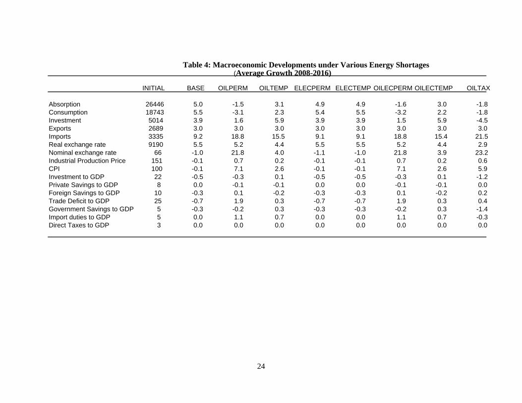
On the demand side of the economy, we also notice that total absorption reduces
by 2 per cent mainly due to the decline in private consumption which declines by
3 per cent. In addition, private investments also grow at a slower rate given the
overall reduction in income levels as will be discussed in the subsequent
sections. Overall, the private savings would decline by 1 per cent of GDP every
year. Notwithstanding the negative effects on private consumption and
investments, the government benefits significantly as its import duties increases
by 1 per cent on an annual basis.
The surge in prices could also put more pressure on the exchange rate as the
country would be faced with a higher import bill that requires more foreign
exchange. This would result into the depreciation of the currency by 5.2 per cent.
The depreciation could indeed be a welcome development especially for
exporters. Indeed we find that exports are boosted by 3 per cent on annual basis
during the period 2008-2012.
There are two main issues regarding the impacts of the increase in oil price.
First, how significant is the increase for the cost of a particular industry as a
result of higher prices of oil. Second, how the output of each industry responds to
cost increases. The oil shock causes devastating impacts across industries.
23
BASE OILPERM OILTEMP ELECPERM ELECTEMP OILECPERM OILECTEMP OILTAX
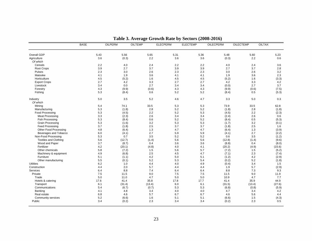
Overall GDP 5.43 5.56 5.65 5.31 5.36 5.48 5.60 5.23 Agriculture 3.6 (0.3) 2.2 3.6 3.6 (0.3) 2.2 0.6 Of which Cereals 2.2 4.0 2.4 2.2 2.2 4.0 2.4 3.6 Root Crops 3.9 2.7 3.7 3.9 3.9 2.7 3.7 2.8 Pulses 2.3 3.0 2.6 2.3 2.3 3.0 2.6 3.2 Matooke 4.1 1.9 3.6 4.1 4.1 1.9 3.6 2.3 Horticulture 4.5 (5.2) 1.6 4.5 4.5 (5.2) 1.6 (3.3) Export Crops 2.7 4.2 3.3 2.7 2.7 4.2 3.3 4.2 Livestock 3.4 0.0 2.7 3.4 3.4 (0.0) 2.7 3.7 Forestry 4.3 (9.9) (0.6) 4.3 4.3 (9.9) (0.6) (7.5) Fishing 5.3 (8.4) 0.6 5.2 5.2 (8.4) 0.5 (5.3)
Industry 5.0 3.5 5.2 4.6 4.7 3.3 5.0 0.3 Of which Mining 5.4 74.1 33.5 5.3 5.3 73.9 33.5 62.8 Manufacturing 5.3 (1.8) 2.8 5.2 5.2 (1.8) 2.8 (1.8) Food Processing 5.3 (4.5) 2.2 5.2 5.3 (4.5) 2.2 (2.3) Meat Processing 3.3 (2.3) 2.6 3.4 3.4 (2.4) 2.6 0.6 Fish Processing 5.3 (8.4) 0.6 5.2 5.2 (8.4) 0.5 (5.3) Grain Processing 5.3 (1.6) 3.2 5.3 5.3 (1.7) 3.2 (0.1) Feed Processing 3.7 (1.8) 2.5 3.7 3.7 (1.8) 2.5 1.6 Other Food Processing 4.8 (6.4) 1.3 4.7 4.7 (6.4) 1.3 (3.9) Beverages and Tobacco 6.0 (4.1) 2.7 5.9 5.9 (4.1) 2.7 (2.2) Non-Food Processing 5.3 0.7 3.5 5.2 5.2 0.6 3.5 (1.2) Textiles and Clothing 5.6 (12.7) (1.4) 5.6 5.6 (12.8) (1.4) (9.6) Wood and Paper 3.7 (8.7) 0.4 3.6 3.6 (8.8) 0.4 (8.0) Fertilizer 4.2 (20.1) (4.8) 4.0 4.1 (20.2) (4.9) (15.6) Other chemicals 5.8 (7.2) 1.5 5.6 5.7 (7.2) 1.5 (5.2) Machinery & equipment 4.9 (6.8) 2.5 4.5 4.7 (7.1) 2.3 (7.4) Furniture 5.1 (1.1) 4.2 5.0 5.1 (1.2) 4.2 (2.9) Other manufacturing 5.5 (0.1) 5.2 5.3 5.4 (0.2) 5.2 (1.8) Utilities 6.2 1.0 4.4 4.0 4.9 (0.4) 3.4 1.5 Construction 4.4 2.0 5.7 4.4 4.4 1.9 5.7 (2.9) Services 6.4 8.8 7.4 6.4 6.4 8.8 7.3 9.3 Private 7.5 11.5 9.0 7.5 7.5 11.5 9.0 11.9 Trade 5.0 11.0 4.7 5.0 5.0 10.9 4.7 7.7 Hotels & catering 17.6 41.4 35.8 17.8 17.7 41.4 35.9 44.9 Transport 6.1 (31.4) (13.4) 6.0 6.1 (31.5) (13.4) (27.6) Communications 5.4 (6.7) (0.7) 5.3 5.3 (6.8) (0.8) (5.9) Banking 4.1 4.8 3.4 4.0 4.0 4.7 3.4 4.2 Real estate 6.8 4.6 5.7 6.7 6.7 4.6 5.6 4.4 Community services 5.2 (6.6) 1.6 5.1 5.1 (6.6) 1.5 (4.3) Public 3.4 (0.2) 2.3 3.4 3.4 (0.2) 2.3 0.5
Table 3. Average Growth Rate by Sectors (2008-2016)
24
INITIAL BASE OILPERM OILTEMP ELECPERM ELECTEMP OILECPERM OILECTEMP OILTAX
Absorption 26446 5.0 -1.5 3.1 4.9 4.9 -1.6 3.0 -1.8Consumption 18743 5.5 -3.1 2.3 5.4 5.5 -3.2 2.2 -1.8Investment 5014 3.9 1.6 5.9 3.9 3.9 1.5 5.9 -4.5Exports 2689 3.0 3.0 3.0 3.0 3.0 3.0 3.0 3.0Imports 3335 9.2 18.8 15.5 9.1 9.1 18.8 15.4 21.5 Real exchange rate 9190 5.5 5.2 4.4 5.5 5.5 5.2 4.4 2.9Nominal exchange rate 66 -1.0 21.8 4.0 -1.1 -1.0 21.8 3.9 23.2 Industrial Production Price 151 -0.1 0.7 0.2 -0.1 -0.1 0.7 0.2 0.6CPI 100 -0.1 7.1 2.6 -0.1 -0.1 7.1 2.6 5.9Investment to GDP 22 -0.5 -0.3 0.1 -0.5 -0.5 -0.3 0.1 -1.2Private Savings to GDP 8 0.0 -0.1 -0.1 0.0 0.0 -0.1 -0.1 0.0Foreign Savings to GDP 10 -0.3 0.1 -0.2 -0.3 -0.3 0.1 -0.2 0.2Trade Deficit to GDP 25 -0.7 1.9 0.3 -0.7 -0.7 1.9 0.3 0.4Government Savings to GDP 5 -0.3 -0.2 0.3 -0.3 -0.3 -0.2 0.3 -1.4Import duties to GDP 5 0.0 1.1 0.7 0.0 0.0 1.1 0.7 -0.3Direct Taxes to GDP 3 0.0 0.0 0.0 0.0 0.0 0.0 0.0 0.0
Table 4: Macroeconomic Developments under Various Energy Shortages(Average Growth 2008-2016)
25
For the case of Uganda, overall we do not see a noticeable change in total GDP.
This is partly because there would be a reallocation of resources between the
sectors with a major boost to trade (which is part of services). However, a detailed
look at the sectoral level reveals a lot more. For instance, for the case of
manufacturing, there would be a total reduction in output of 7 per cent during the
period 2008-12. This output loss is witnessed amongst all the subcategories
including both the agro-processing and non-agro-processing industries. There are
several explanations for this. First, the manufacturing sector relies a lot on transport
so this becomes an increased cost in the process of production. Second, a lot of
factories are now relying on generators owing to the frequent power outages.
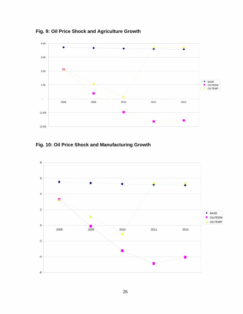
Also of interest is that the agricultural sector is also affected. The total output loss
due to the permanent price increase is estimated at 0.3 per cent of GDP over the
period 2008-12. Agriculture depends a lot on the transportation sector especially
while transporting goods to the intended markets. However, within agriculture, we
find that the horticulture industry is most affected owing to the heavy use of
generators for this industry. Also, the heavy use of transport and generators is
portrayed for the fishing industry which declines by 8.4 per cent due to higher oil
prices.4
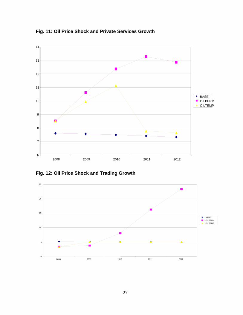
The overall impact on services is positive. However, it’s important again to scrutinize
the individual sectors in services. Transport which is so dependent on oil is the worst
affected. Overall we notice that the output of transport would decline by 30 per cent.
This is substantial given that there are so many other sectors that are dependent on
the transportation sector. On the other hand, trade would be significantly boosted as
a result of the fluctuations in oil prices. Indeed for the case of Uganda, this is
evidenced by the high number of petrol stations being opened.
4 The increase in production costs due to high oil prices, high electricity tariffs and reduction of stocks of fish in Lake Victoria partly explains the recent bankruptcies and closure of several fish factories.
26
Fig. 9: Oil Price Shock and Agriculture Growth
Fig. 10: Oil Price Shock and Manufacturing Growth
-6
-4
-2
0
2
4
6
8
2008 2009 2010 2011 2012
BASEOILPERMOILTEMP
(2.00)
(1.00)
-
1.00
2.00
3.00
4.00
2008 2009 2010 2011 2012
BASEOILPERMOILTEMP
27
Fig. 11: Oil Price Shock and Private Services Growth
Fig. 12: Oil Price Shock and Trading Growth
0
5
10
15
20
25
2008 2009 2010 2011 2012
BASEOILPERMOILTEMP
6
7
8
9
10
11
12
13
14
2008 2009 2010 2011 2012
BASEOILPERMOILTEMP
28
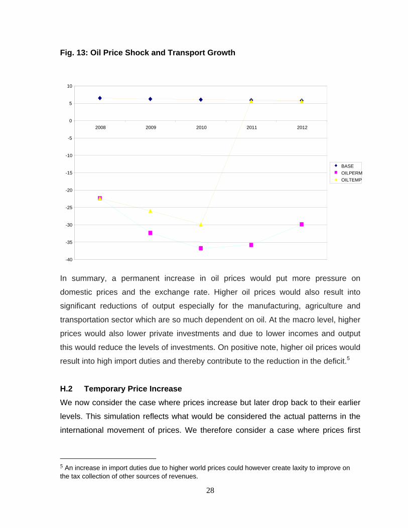
Fig. 13: Oil Price Shock and Transport Growth
In summary, a permanent increase in oil prices would put more pressure on
domestic prices and the exchange rate. Higher oil prices would also result into
significant reductions of output especially for the manufacturing, agriculture and
transportation sector which are so much dependent on oil. At the macro level, higher
prices would also lower private investments and due to lower incomes and output
this would reduce the levels of investments. On positive note, higher oil prices would
result into high import duties and thereby contribute to the reduction in the deficit.5
H.2 Temporary Price Increase We now consider the case where prices increase but later drop back to their earlier
levels. This simulation reflects what would be considered the actual patterns in the
international movement of prices. We therefore consider a case where prices first
5 An increase in import duties due to higher world prices could however create laxity to improve on the tax collection of other sources of revenues.
-40
-35
-30
-25
-20
-15
-10
-5
0
5
10
2008 2009 2010 2011 2012
BASEOILPERMOILTEMP
29
increase by 50 per cent during 2008 and in the subsequent years start falling back to
the original levels.
From a macro perspective, the effects of a temporary increase in oil prices are very
different from the permanent case scenario. In general, the effects would not be as
negative compared to the earlier results. The CPI would only increase during the
year we witness a price surge, but prices would ten normalize back to the original
levels.
On the demand side of the economy, total absorption is much higher than for the
permanent increase but still lower than the baseline where prices do not change at
all. The change in total absorption is a reflection of the reduction in private
consumption during the year when prices increase significantly. The pressure that is
put on the exchange rate is also less with the currency only depreciating by 5 per
cent per year.
The overall impact of a temporary increase in prices of oil also depends so much on
the sector in question. For the case of manufacturing, there would be a total
reduction in output of 2.2 per cent during the period 2008-12. This is much lower
output loss to the economy compared to the previous scenario. This output loss is
also witnessed amongst all the subcategories including both the agro-processing
and non agro-processing industries. Likewise transport which is so dependent on oil
would be negatively affected but the effect would be subdued.
This simulation reveals that the government should indeed intervene with the traders
of oil products in Uganda in the event that it’s the case that they manipulate prices.
Indeed, there is considerable output to be gained if prices were being adjusted in
line with international crude oil prices. While there could be other reasons why prices
have remained high, government should come up with a clear policy on price of oil
vis-à-vis the international prices.
30
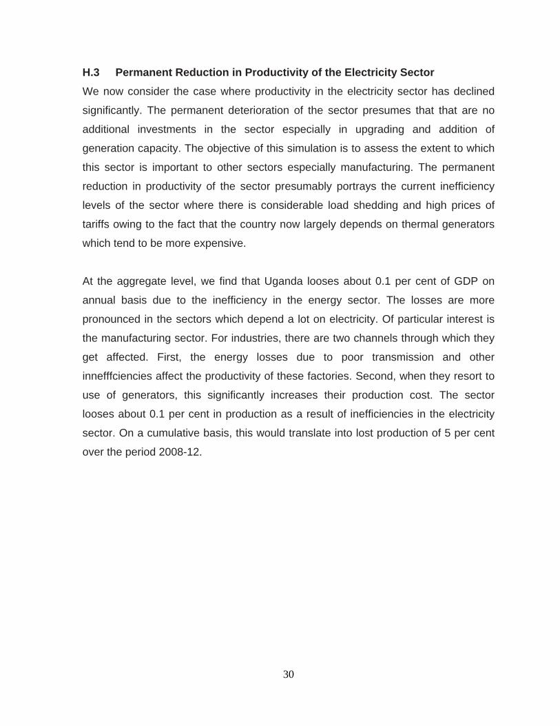
H.3 Permanent Reduction in Productivity of the Electricity Sector We now consider the case where productivity in the electricity sector has declined
significantly. The permanent deterioration of the sector presumes that that are no
additional investments in the sector especially in upgrading and addition of
generation capacity. The objective of this simulation is to assess the extent to which
this sector is important to other sectors especially manufacturing. The permanent
reduction in productivity of the sector presumably portrays the current inefficiency
levels of the sector where there is considerable load shedding and high prices of
tariffs owing to the fact that the country now largely depends on thermal generators
which tend to be more expensive.
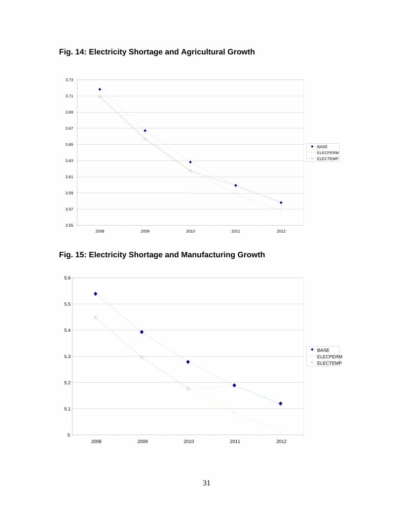
At the aggregate level, we find that Uganda looses about 0.1 per cent of GDP on
annual basis due to the inefficiency in the energy sector. The losses are more
pronounced in the sectors which depend a lot on electricity. Of particular interest is
the manufacturing sector. For industries, there are two channels through which they
get affected. First, the energy losses due to poor transmission and other
innefffciencies affect the productivity of these factories. Second, when they resort to
use of generators, this significantly increases their production cost. The sector
looses about 0.1 per cent in production as a result of inefficiencies in the electricity
sector. On a cumulative basis, this would translate into lost production of 5 per cent
over the period 2008-12.
31
Fig. 14: Electricity Shortage and Agricultural Growth
Fig. 15: Electricity Shortage and Manufacturing Growth
5
5.1
5.2
5.3
5.4
5.5
5.6
2008 2009 2010 2011 2012
BASEELECPERMELECTEMP
3.55
3.57
3.59
3.61
3.63
3.65
3.67
3.69
3.71
3.73
2008 2009 2010 2011 2012
BASEELECPERMELECTEMP
32
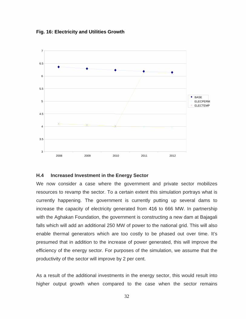
Fig. 16: Electricity and Utilities Growth
H.4 Increased Investment in the Energy Sector We now consider a case where the government and private sector mobilizes
resources to revamp the sector. To a certain extent this simulation portrays what is
currently happening. The government is currently putting up several dams to
increase the capacity of electricity generated from 416 to 666 MW. In partnership
with the Aghakan Foundation, the government is constructing a new dam at Bajagali
falls which will add an additional 250 MW of power to the national grid. This will also
enable thermal generators which are too costly to be phased out over time. It’s
presumed that in addition to the increase of power generated, this will improve the
efficiency of the energy sector. For purposes of the simulation, we assume that the
productivity of the sector will improve by 2 per cent.
As a result of the additional investments in the energy sector, this would result into
higher output growth when compared to the case when the sector remains
3
3.5
4
4.5
5
5.5
6
6.5
7
2008 2009 2010 2011 2012
BASEELECPERMELECTEMP
33
inefficient, the country can recover more than 5 per cent growth in GDP over the
period 2009-2012. The recovery would mainly come from the sector itself and other
sectors that use electricity as an intermediate input. The specific sectors like
manufacturing would also be able to produce at a higher rate. This shows that there
is a lot to gain when more investments are tailored to the sector.
H.5 Removal of Tariffs on Oil Commodities From a policy perspective, the government could circumvent the increase in the oil
prices by reducing the tariffs. However, before ascertaining whether this is the ideal
option, we need to understand the impact of an oil shock on the demand. First, an oil
price increase could potentially result into a decline in total demand for oil products.
On the other hand there would be a value increase owing to the nominal price
change. Therefore, while there would be an increase in the price the quantity
demanded could actually drop resulting into an overall decline in value. Hence the
reduction in tariff could indeed reduce the domestic price level which would stimulate
further demand for oil.
From the simulation, we reduce tariffs by 50 per cent. This has several
macroeconomic consequences. First, there is a direct loss in tariff revenues which
results into a higher deficit. By running higher deficits which would require financing
by the government results into crowding out of resources and reduces private
investments by 1 per cent on an annual basis. However, this policy would
circumvent some of the output losses at a sectoral level only in the short run. For
instance the losses in agriculture and industry are less than when government does
nothing. The benefits are short-lived though owing to the fact that the high deficits
run by the central government would catch up with the private sector. From the
consumption side, the households would also temporarily benefit in the year when
the tariff reduction is implemented.
34
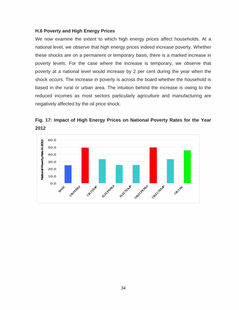
H.6 Poverty and High Energy Prices We now examine the extent to which high energy prices affect households. At a
national level, we observe that high energy prices indeed increase poverty. Whether
these shocks are on a permanent or temporary basis, there is a marked increase in
poverty levels. For the case where the increase is temporary, we observe that
poverty at a national level would increase by 2 per cent during the year when the
shock occurs. The increase in poverty is across the board whether the household is
based in the rural or urban area. The intuition behind the increase is owing to the
reduced incomes as most sectors particularly agriculture and manufacturing are
negatively affected by the oil price shock.
Fig. 17: Impact of High Energy Prices on National Poverty Rates for the Year 2012
0.0
10.0
20.0
30.0
40.0
50.0
60.0
BASE
OILPERM
OILTEMP
ELECPERM
ELECTEMP
OILECPERM
OILECTEMP
OILTAX
National Poverty Rate in 2012
35
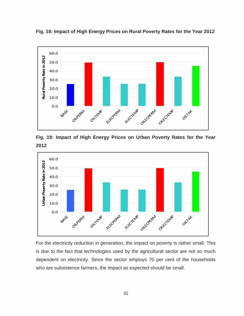
Fig. 18: Impact of High Energy Prices on Rural Poverty Rates for the Year 2012
Fig. 19: Impact of High Energy Prices on Urban Poverty Rates for the Year 2012
For the electricity reduction in generation, the impact on poverty is rather small. This
is due to the fact that technologies used by the agricultural sector are not so much
dependent on electricity. Since the sector employs 70 per cent of the households
who are subsistence farmers, the impact as expected should be small.
0.0
10.0
20.0
30.0
40.0
50.0
60.0
BASE
OILPERM
OILTEMP
ELECPERM
ELECTEMP
OILECPERM
OILECTEMP
OILTAX
Rural Poverty Rate in 2012
0.0
10.0
20.0
30.0
40.0
50.0
60.0
BASE
OILPERM
OILTEMP
ELECPERM
ELECTEMP
OILECPERM
OILECTEMP
OILTAX
Urban Poverty Rate in 2012
36
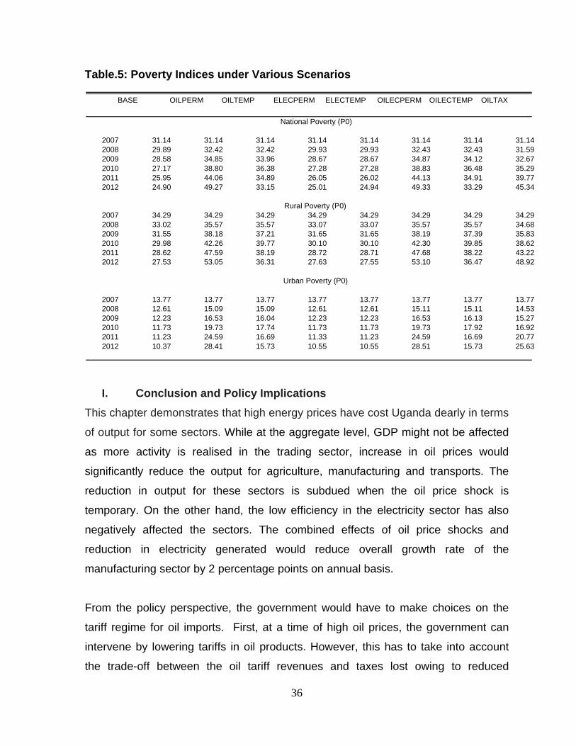
Table.5: Poverty Indices under Various Scenarios
I. Conclusion and Policy Implications This chapter demonstrates that high energy prices have cost Uganda dearly in terms
of output for some sectors. While at the aggregate level, GDP might not be affected
as more activity is realised in the trading sector, increase in oil prices would
significantly reduce the output for agriculture, manufacturing and transports. The
reduction in output for these sectors is subdued when the oil price shock is
temporary. On the other hand, the low efficiency in the electricity sector has also
negatively affected the sectors. The combined effects of oil price shocks and
reduction in electricity generated would reduce overall growth rate of the
manufacturing sector by 2 percentage points on annual basis.
From the policy perspective, the government would have to make choices on the
tariff regime for oil imports. First, at a time of high oil prices, the government can
intervene by lowering tariffs in oil products. However, this has to take into account
the trade-off between the oil tariff revenues and taxes lost owing to reduced
BASE OILPERM OILTEMP ELECPERM ELECTEMP OILECPERM OILECTEMP OILTAX
2007 31.14 31.14 31.14 31.14 31.14 31.14 31.14 31.142008 29.89 32.42 32.42 29.93 29.93 32.43 32.43 31.592009 28.58 34.85 33.96 28.67 28.67 34.87 34.12 32.672010 27.17 38.80 36.38 27.28 27.28 38.83 36.48 35.292011 25.95 44.06 34.89 26.05 26.02 44.13 34.91 39.772012 24.90 49.27 33.15 25.01 24.94 49.33 33.29 45.34
2007 34.29 34.29 34.29 34.29 34.29 34.29 34.29 34.292008 33.02 35.57 35.57 33.07 33.07 35.57 35.57 34.682009 31.55 38.18 37.21 31.65 31.65 38.19 37.39 35.832010 29.98 42.26 39.77 30.10 30.10 42.30 39.85 38.622011 28.62 47.59 38.19 28.72 28.71 47.68 38.22 43.222012 27.53 53.05 36.31 27.63 27.55 53.10 36.47 48.92
2007 13.77 13.77 13.77 13.77 13.77 13.77 13.77 13.772008 12.61 15.09 15.09 12.61 12.61 15.11 15.11 14.532009 12.23 16.53 16.04 12.23 12.23 16.53 16.13 15.272010 11.73 19.73 17.74 11.73 11.73 19.73 17.92 16.922011 11.23 24.59 16.69 11.33 11.23 24.59 16.69 20.772012 10.37 28.41 15.73 10.55 10.55 28.51 15.73 25.63
Rural Poverty (P0)
National Poverty (P0)
Urban Poverty (P0)
37
economic activity especially in the manufacturing sector. Second, the government
should take a more active role on suppliers to ensure that prices are adjusted
downwards when international prices drop. Whereas it is possible that lack of quick
transmission of lower prices at the international level to the domestic market may be
due to the physical bottlenecks alluded to in section B3, the inability of the players in
the industry to reduce prices after months of a drop in international crude prices
point more to an institutional problem that may be under the control of the
government to address. As found, the output losses are much higher when the price
increase remains permanent. Third, without addressing the inefficiencies in the
electricity sector, this will continue affecting the output of manufacturing and other
sectors that depend on electricity. More private-public investments should be
encouraged to enhance the productivity and capacity of the sector.
38
Reference
Abeysinghe, T., (2001). “Estimation of direct and indirect impact of oil price on growth”, Department of Economics, National University of Singapore, 10 Kent Ridge Crescent, Singapore 119260, Singapore
Adenikinju, A. F., and Falobi, N., (2006). “Macroeconomic and distributional
consequences of energy supply shocks in Nigeria” AERC Research Paper 162 African Economic Research Consortium, Nairobi
Bacon, R., and Mattar, A., (2005). “The Vulnerability of African Countries to Oil Price
Shocks: Major Factors and Policy Options: The Case of Oil Importing Countries”, Energy Sector Management Assistance Programme (ESMAP), World Bank, Washington, DC
Carlstrom, C., T., and Fuerst, T., S., (2005). “Oil Prices, Monetary Policy, and the
Macroeconomy” Federal Reserve Bank of Cleveland, Policy Discussion Papers Number 10
Ciscar, J. C., P. Russ, L., Parousos and Stroblos, N., (2004). “Vulnerability of the EU
Economy to Oil Shocks: A General equilibrium Analysis with the GEM-E3 Model”. Paper presented at the 13th annual conference of the European Association of Environmental and Resource Economics, Budapest, Hungary.
Energy Information Administration (EIA), (2008). Official Energy Statistics from the
US Government Guha, G. S., (2005). “Simulation of the Economic Impact of Region-wide Electricity
Outages from a Natural Hazard Using a CGE Model,” Southwestern Economic Review, 32(1): 101–124
Hope, E., and Singh, B., ( 199..). “Energy Price Increases in Developing Countries
Case Studies of Colombia, Ghana, Indonesia, Malaysia, Turkey, and Zimbabwe”, The World Bank Public Economics Division
Hunt, B., Isard, P., and Laxton D., (2001). “The macroeconomic Effects of Higher
Oil Prices” Kojima, M., and Bacon, R., (2006). “Coping with Higher Oil Prices”, Energy Sector
Management Assistance Programme (ESMAP), World Bank, Washington, DC Lee, K., and Ni, S., (2002). “On the Dynamic Effects of Oil Price Shocks: A Study
Using Industry Level Data,” Journal of Monetary Economics 49: 823-852.
39
Nkomo J. C (2006) “The impact of higher oil prices on Southern African countries” Energy Research Centre, University of Cape Town Journal of Energy in Southern Africa, Vol 17 No 1
Pradhan, B. K., and Sahoo, A., (2000). “Oil Price Shocks and Poverty in a CGE
Framework” National Council of Applied Economic Research, 11 - I.P. Estate, New Delhi
PROVIDE (2005). “A Computable General Equilibrium (CGE) Analysis of the impact
of an Oil Price Increase in South Africa” PROVIDE Working Paper 2005 Schneider, M., (2004). “The Impact of Oil Price Changes on Growth and Inflation” Monetary Policy & the Economy Q2/04 _ 27 Uganda Bureau of Statistics (2007), 2007 Statistical Abstract, Kampala.
40
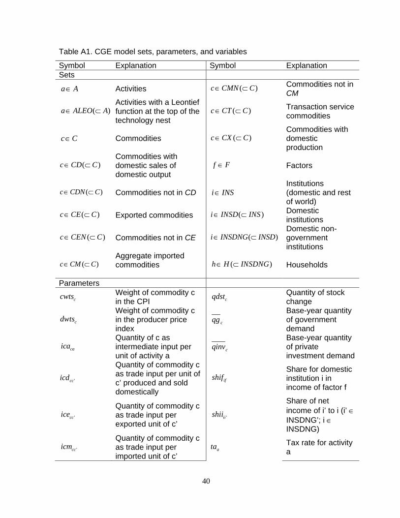
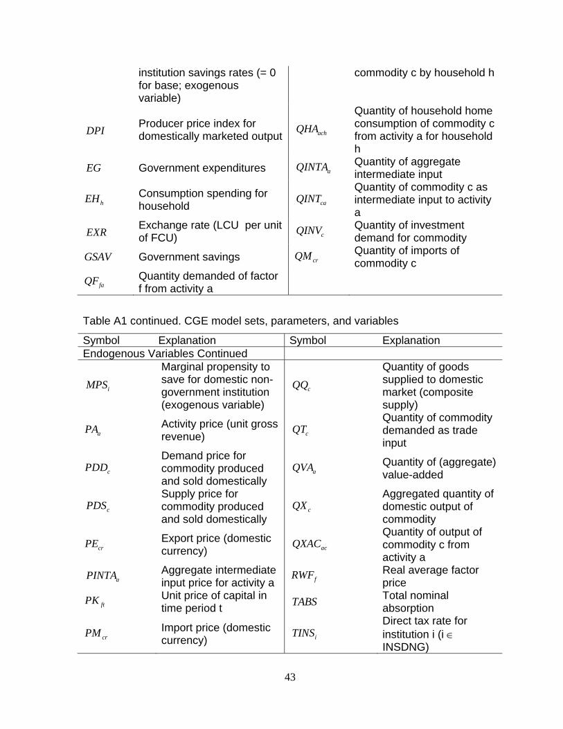
Table A1. CGE model sets, parameters, and variables
Symbol Explanation Symbol Explanation Sets
Activities Commodities not in CM
Activities with a Leontief function at the top of the technology nest
Transaction service commodities
Commodities Commodities with domestic production
Commodities with domestic sales of domestic output
Factors
Commodities not in CD Institutions (domestic and rest of world)
Exported commodities Domestic institutions
Commodities not in CE Domestic non-government institutions
( )c CM C∈ ⊂ Aggregate imported commodities
Households
Parameters
Weight of commodity c in the CPI
Quantity of stock change
Weight of commodity c in the producer price index
Base-year quantity of government demand
Quantity of c as intermediate input per unit of activity a
Base-year quantity of private investment demand
Quantity of commodity c as trade input per unit of c’ produced and sold domestically
Share for domestic institution i in income of factor f
Quantity of commodity c as trade input per exported unit of c’
Share of net income of i’ to i (i’ ∈ INSDNG’; i ∈ INSDNG)
Quantity of commodity c as trade input per imported unit of c’
Tax rate for activity a
a A∈ ( )c CMN C∈ ⊂
( )a ALEO A∈ ⊂ ( )c CT C∈ ⊂
c C∈ ( )c CX C∈ ⊂
( )c CD C∈ ⊂ f F∈
( )c CDN C∈ ⊂ i INS∈
( )c CE C∈ ⊂ ( )i INSD INS∈ ⊂
( )c CEN C∈ ⊂ ( )i INSDNG INSD∈ ⊂
( )h H INSDNG∈ ⊂
ccwts cqdst
cdwts cqg
caica cqinv
'ccicd ifshif
'ccice 'iishii
'ccicm ata

41
Quantity of aggregate intermediate input per activity unit
Exogenous direct tax rate for domestic institution i
Quantity of aggregate intermediate input per activity unit
0-1 parameter with 1 for institutions with potentially flexed direct tax rates
Base savings rate for domestic institution i
Import tariff rate
0-1 parameter with 1 for institutions with potentially flexed direct tax rates
Rate of sales tax
Export price (foreign currency)
Transfer from factor f to institution i
Import price (foreign currency)
ainta itins
aiva itins01
imps ctm
imps01 ctq
cpwe i ftrnsfr
cpwm
42
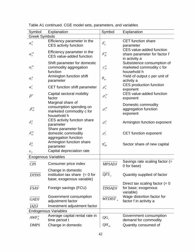
Table A1 continued. CGE model sets, parameters, and variables
Symbol Explanation Symbol Explanation Greek Symbols
Efficiency parameter in the CES activity function
tcrδ CET function share
parameter
Efficiency parameter in the CES value-added function
CES value-added function share parameter for factor f in activity a
Shift parameter for domestic commodity aggregation function
Subsistence consumption of marketed commodity c for household h
Armington function shift parameter
Yield of output c per unit of activity a
CET function shift parameter CES production function exponent
aβ Capital sectoral mobility factor CES value-added function
exponent
Marginal share of consumption spending on marketed commodity c for household h
Domestic commodity aggregation function exponent
CES activity function share parameter Armington function exponent
Share parameter for domestic commodity aggregation function
CET function exponent
qcrδ Armington function share
parameter afatη Sector share of new capital
fυ Capital depreciation rate Exogenous Variables
Consumer price index Savings rate scaling factor (= 0 for base)
Change in domestic institution tax share (= 0 for base; exogenous variable)
Quantity supplied of factor
Foreign savings (FCU) Direct tax scaling factor (= 0 for base; exogenous variable)
Government consumption adjustment factor
Wage distortion factor for factor f in activity a
Investment adjustment factor Endogenous Variables
aftAWF
Average capital rental rate in time period t
Government consumption demand for commodity
Change in domestic Quantity consumed of
aaα
vaaα
vafaδ
accα
mchγ
qcα acθ
tcα
aaρ
vaaρ
mchβ ac
cρ
aaδ
qcρ
acacδ t
cρ
CPI MPSADJ
DTINS fQFS
FSAV TINSADJ
GADJ faWFDIST
IADJ
cQG
DMPS chQH
43
institution savings rates (= 0 for base; exogenous variable)
commodity c by household h
Producer price index for domestically marketed output
Quantity of household home consumption of commodity c from activity a for household h
Government expenditures Quantity of aggregate intermediate input
Consumption spending for household
Quantity of commodity c as intermediate input to activity a
Exchange rate (LCU per unit of FCU)
Quantity of investment demand for commodity
Government savings crQM Quantity of imports of commodity c
Quantity demanded of factor f from activity a
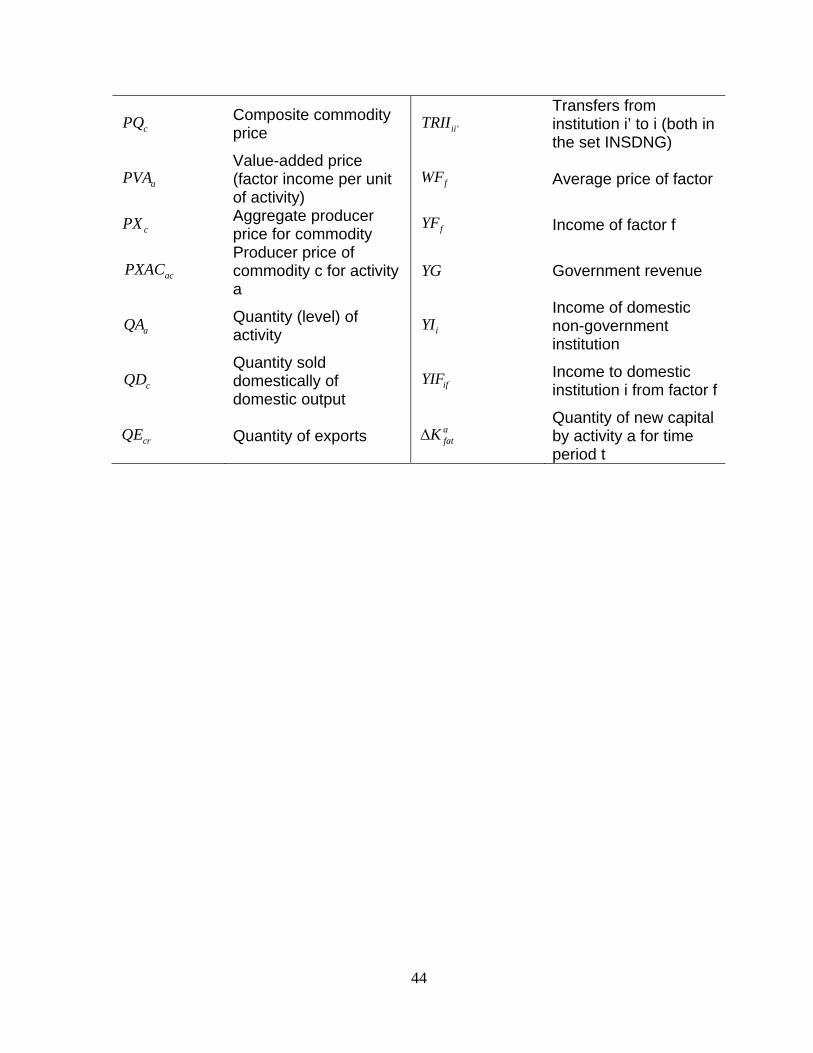
Table A1 continued. CGE model sets, parameters, and variables
Symbol Explanation Symbol Explanation Endogenous Variables Continued
Marginal propensity to save for domestic non-government institution (exogenous variable)
Quantity of goods supplied to domestic market (composite supply)
Activity price (unit gross revenue)
Quantity of commodity demanded as trade input
Demand price for commodity produced and sold domestically
Quantity of (aggregate) value-added
Supply price for commodity produced and sold domestically
Aggregated quantity of domestic output of commodity
crPE Export price (domestic currency)
Quantity of output of commodity c from activity a
Aggregate intermediate input price for activity a fRWF Real average factor
price
ftPK Unit price of capital in time period t Total nominal
absorption
crPM Import price (domestic currency)
Direct tax rate for institution i (i ∈ INSDNG)
DPI achQHA
EG aQINTA
hEH caQINT
EXR cQINV
GSAV
faQF
iMPS cQQ
aPA cQT
cPDD aQVA
cPDS cQX
acQXAC
aPINTA
TABS
iTINS
44
Composite commodity price
Transfers from institution i’ to i (both in the set INSDNG)
Value-added price (factor income per unit of activity)
Average price of factor
Aggregate producer price for commodity
Income of factor f
Producer price of commodity c for activity a
Government revenue
Quantity (level) of activity
Income of domestic non-government institution
Quantity sold domestically of domestic output
Income to domestic institution i from factor f
crQE Quantity of exports afatKΔ
Quantity of new capital by activity a for time period t
cPQ 'iiTRII
aPVA fWF
cPX fYF
acPXAC YG
aQA iYI
cQD ifYIF
45
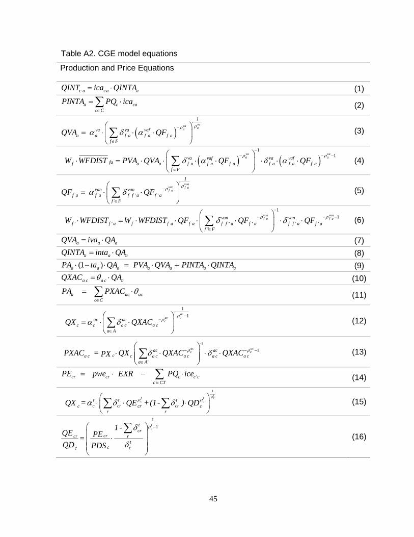
Table A2. CGE model equations
Production and Price Equations
c a c a aQINT ica QINTA= ⋅ (1)
a c cac C
PINTA PQ ica∈
= ⋅∑ (2)
( )vava aa
1-
va va vafa a f a f a f a
f FQVA QF
ρρα δ α
−
∈
⎛ ⎞= ⋅ ⋅ ⋅⎜ ⎟
⎝ ⎠∑ (3)
( ) ( )1
1
'
va vaa ava vaf va vaf
faf a a f a f a f a f a f a f af F
W WFDIST PVA QVA QF QFρ ρ
δ α δ α−
− − −
∈
⎛ ⎞⋅ = ⋅ ⋅ ⋅ ⋅ ⋅ ⋅ ⋅⎜ ⎟
⎝ ⎠∑ (4)
' ''
vanvan f af a
1-
van vanf a f a f f a f a
f FQF QF
ρρα δ −
∈
⎛ ⎞= ⋅ ⋅⎜ ⎟
⎝ ⎠∑ (5)
11
' ' '' '' ' '''
van vanf a f avan van
f f a f f a f a f f a f a f f a f af F
W WFDIST W WFDIST QF QF QFρ ρδ δ−
− − −
∈
⎛ ⎞⋅ = ⋅ ⋅ ⋅ ⋅ ⋅ ⋅⎜ ⎟
⎝ ⎠∑ (6)
a a aQVA iva QA= ⋅ (7)
a a aQINTA inta QA= ⋅ (8) (1 )a a a a a a aPA ta QA PVA QVA PINTA QINTA⋅ − ⋅ = ⋅ + ⋅ (9)
a c a c aQXAC QAθ= ⋅ (10)
a ac acc C
PA PXAC θ∈
= ⋅∑ (11)1
1accac
cac acc c a c a c
a AQX QXAC
ρρα δ
−−
−
∈
⎛ ⎞= ⋅ ⋅⎜ ⎟
⎝ ⎠∑ (12)
1
1
'
ac acc cac ac
ca c c a c a c a c a ca A
PXAC = QX QXAC QXACPX ρ ρδ δ−
− − −
∈
⎛ ⎞⋅ ⋅ ⋅ ⋅⎜ ⎟⎜ ⎟
⎝ ⎠∑ (13)
''
cr cr c c cc CT
PE pwe EXR PQ ice∈
= ⋅ − ⋅∑ (14)1tct t
c ct t tc cr crc cr c
r r = + (1- )QX QE QD
ρρ ρα δ δ⎛ ⎞⋅ ⋅ ⋅⎜ ⎟
⎝ ⎠∑ ∑ (15)
11t
ctcr
crcr rt
c cc
1 - QE PE = QD PDS
ρδ
δ
−⎛ ⎞⎜ ⎟⋅⎜ ⎟⎜ ⎟⎝ ⎠
∑ (16)
46
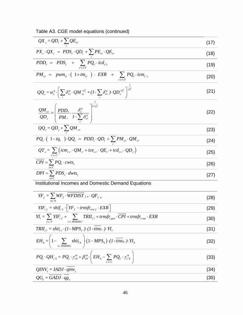
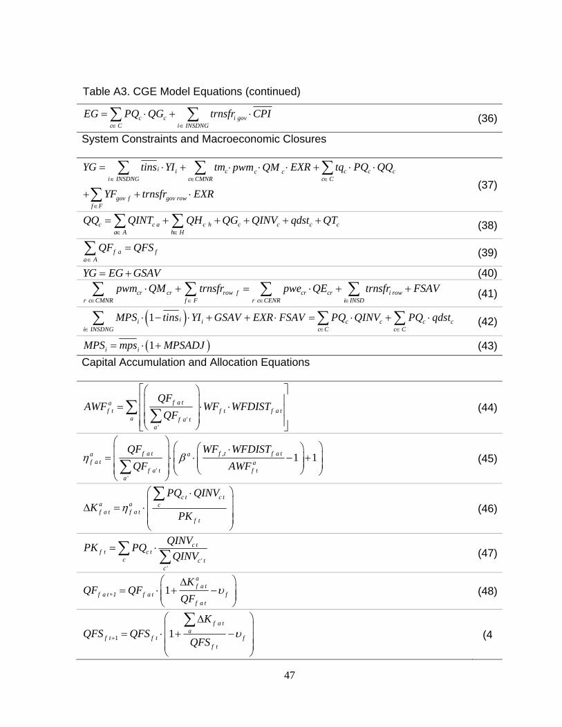
Table A3. CGE model equations (continued)
c crcr
= QD QEQX +∑ (17)
c c c c cr crr
PX QX PDS QD PE QE⋅ = ⋅ + ⋅∑ (18)
' ''
c c c c cc CT
PDD PDS PQ icd∈
= + ⋅∑ (19)
( ) ' ''
1cr cr cr c c cc CT
PM pwm tm EXR PQ icm∈
= ⋅ + ⋅ + ⋅∑ (20)
qq q cc c
1-- -q q q
c cr crc cr cr r
= + (1- )QQ QM QDρρ ρα δ δ⎛ ⎞
⋅ ⋅ ⋅⎜ ⎟⎝ ⎠∑ ∑ (21)
qc
11+
qccr c
qc crc
r
QM PDD =1 - QD PM
ρδ
δ
⎛ ⎞⎜ ⎟⋅⎜ ⎟⎜ ⎟⎝ ⎠
∑ (22)
c c crr
= QQ QD QM+∑ (23)
( )1c c c c c cr crr
PQ tq QQ PDD QD PM QM⋅ − ⋅ = ⋅ + ⋅∑ (24)
( )' ' ' ' ' '' '
c c c c c c c cc cc C
= icm QM ice QE icd QT QD∈
⋅ + ⋅ + ⋅∑ (25)
c cc C
CPI PQ cwts∈
= ⋅∑ (26)
c cc C
DPI PDS dwts∈
= ⋅∑ (27)
Institutional Incomes and Domestic Demand Equations
f af f f aa A
YF = WF WFDIST QF∈
⋅ ⋅∑ (28)
i f i f f row fYIF = shif YF trnsfr EXR⎡ ⎤⋅ − ⋅⎣ ⎦ (29)
'' '
i i f i i i gov i rowf F i INSDNG
YI = YIF TRII trnsfr CPI trnsfr EXR∈ ∈
+ + ⋅ + ⋅∑ ∑ (30)
'' ' ' 'ii i i i i iTRII = shii (1- MPS ) (1- tins ) YI⋅ ⋅ ⋅ (31)
( )1 1 hh i h h hi INSDNG
EH = shii MPS (1- tins ) YI∈
⎛ ⎞− ⋅ − ⋅ ⋅⎜ ⎟
⎝ ⎠∑ (32)
' ''
m m mc c h c ch ch h c c h
c CPQ QH = PQ EH PQγ β γ
∈
⎛ ⎞⋅ ⋅ + ⋅ − ⋅⎜ ⎟
⎝ ⎠∑ (33)
c cQINV = IADJ qinv⋅ (34)
c cQG = GADJ qg⋅ (35)
47
Table A3. CGE Model Equations (continued)
c c i govc C i INSDNG
EG PQ QG trnsfr CPI∈ ∈
= ⋅ + ⋅∑ ∑ (36)
System Constraints and Macroeconomic Closures
i i c c c cc ci INSDNG c CMNR c C
gov f gov rowf F
YG tins YI tm EXR tq PQ QQpwm QM
YF trnsfr EXR∈ ∈ ∈
∈
= ⋅ + ⋅ ⋅ + ⋅ ⋅⋅
+ + ⋅
∑ ∑ ∑
∑ (37)
c c a c h c c c ca A h H
QQ QINT QH QG QINV qdst QT∈ ∈
= + + + + +∑ ∑ (38)
f a fa A
QF QFS∈
=∑ (39)
YG EG GSAV= + (40)cr cr row f cr cr i row
r c CMNR f F r c CENR i INSDpwm QM trnsfr pwe QE trnsfr FSAV
∈ ∈ ∈ ∈
⋅ + = ⋅ + +∑ ∑ ∑ ∑ (41)
( )1 ii i c c c ci INSDNG c C c C
MPS tins YI GSAV EXR FSAV PQ QINV PQ qdst∈ ∈ ∈
⋅ − ⋅ + + ⋅ = ⋅ + ⋅∑ ∑ ∑ (42)
( )1i iMPS mps MPSADJ= ⋅ + (43)Capital Accumulation and Allocation Equations
'
f a taf t f t f a t
a f a' ta
QFAWF WF WFDIST
QF
⎡ ⎤⎛ ⎞⎢ ⎥⎜ ⎟= ⋅ ⋅⎢ ⎥⎜ ⎟⎜ ⎟⎢ ⎥⎝ ⎠⎣ ⎦
∑ ∑ (44)
,
'
1 1f a t f t f a ta af a t a
f a' t f ta
QF WF WFDISTQF AWF
η β⎛ ⎞ ⎛ ⎞⎛ ⎞⋅⎜ ⎟= ⋅ ⋅ − +⎜ ⎟⎜ ⎟⎜ ⎟ ⎜ ⎟⎜ ⎟⎜ ⎟ ⎝ ⎠⎝ ⎠⎝ ⎠∑
(45)
c t c ta a cf a t f a t
f t
PQ QINVK
PKη
⎛ ⎞⋅⎜ ⎟Δ = ⋅⎜ ⎟⎜ ⎟⎝ ⎠
∑ (46)
'
c tf t c t
c c' tc
QINVPK PQQINV
= ⋅∑ ∑ (47)
1af a t
f a t+1 f a t ff a t
KQF QF
QFυ
⎛ ⎞Δ= ⋅ + −⎜ ⎟⎜ ⎟
⎝ ⎠ (48)
1 1f a t
af t f t f
f t
KQFS QFS
QFSυ+
⎛ ⎞Δ⎜ ⎟= ⋅ + −⎜ ⎟⎜ ⎟⎝ ⎠
∑ (4
48
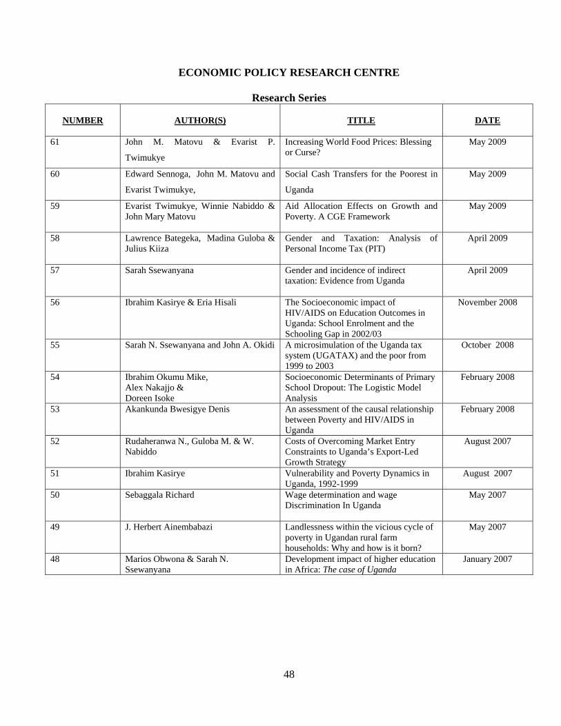
ECONOMIC POLICY RESEARCH CENTRE
Research Series
NUMBER
AUTHOR(S)
TITLE
DATE
61 John M. Matovu & Evarist P.
Twimukye
Increasing World Food Prices: Blessing or Curse?
May 2009
60 Edward Sennoga, John M. Matovu and
Evarist Twimukye,
Social Cash Transfers for the Poorest in
Uganda
May 2009
59 Evarist Twimukye, Winnie Nabiddo & John Mary Matovu
Aid Allocation Effects on Growth and Poverty. A CGE Framework
May 2009
58 Lawrence Bategeka, Madina Guloba & Julius Kiiza
Gender and Taxation: Analysis of Personal Income Tax (PIT)
April 2009
57 Sarah Ssewanyana
Gender and incidence of indirect taxation: Evidence from Uganda
April 2009
56 Ibrahim Kasirye & Eria Hisali The Socioeconomic impact of HIV/AIDS on Education Outcomes in Uganda: School Enrolment and the Schooling Gap in 2002/03
November 2008
55 Sarah N. Ssewanyana and John A. Okidi A microsimulation of the Uganda tax system (UGATAX) and the poor from 1999 to 2003
October 2008
54 Ibrahim Okumu Mike, Alex Nakajjo & Doreen Isoke
Socioeconomic Determinants of Primary School Dropout: The Logistic Model Analysis
February 2008
53 Akankunda Bwesigye Denis
An assessment of the causal relationship between Poverty and HIV/AIDS in Uganda
February 2008
52 Rudaheranwa N., Guloba M. & W. Nabiddo
Costs of Overcoming Market Entry Constraints to Uganda’s Export-Led Growth Strategy
August 2007
51 Ibrahim Kasirye Vulnerability and Poverty Dynamics in Uganda, 1992-1999
August 2007
50 Sebaggala Richard
Wage determination and wage Discrimination In Uganda
May 2007
49 J. Herbert Ainembabazi
Landlessness within the vicious cycle of poverty in Ugandan rural farm households: Why and how is it born?
May 2007
48 Marios Obwona & Sarah N. Ssewanyana
Development impact of higher education in Africa: The case of Uganda
January 2007
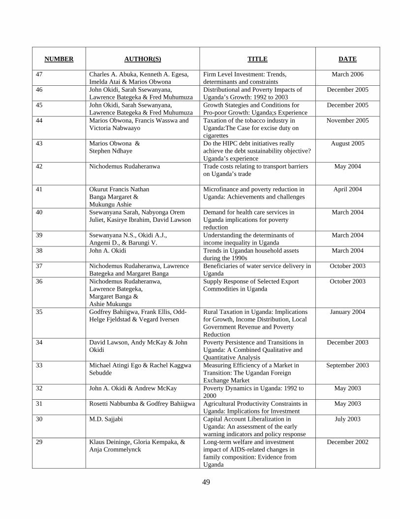
49
NUMBER
AUTHOR(S)
TITLE
DATE
47 Charles A. Abuka, Kenneth A. Egesa, Imelda Atai & Marios Obwona
Firm Level Investment: Trends, determinants and constraints
March 2006
46 John Okidi, Sarah Ssewanyana, Lawrence Bategeka & Fred Muhumuza
Distributional and Poverty Impacts of Uganda’s Growth: 1992 to 2003
December 2005
45 John Okidi, Sarah Ssewanyana, Lawrence Bategeka & Fred Muhumuza
Growth Stategies and Conditions for Pro-poor Growth: Uganda;s Experience
December 2005
44 Marios Obwona, Francis Wasswa and Victoria Nabwaayo
Taxation of the tobacco industry in Uganda:The Case for excise duty on cigarettes
November 2005
43 Marios Obwona & Stephen Ndhaye
Do the HIPC debt initiatives really achieve the debt sustainability objective? Uganda’s experience
August 2005
42 Nichodemus Rudaheranwa
Trade costs relating to transport barriers on Uganda’s trade
May 2004
41 Okurut Francis Nathan Banga Margaret & Mukungu Ashie
Microfinance and poverty reduction in Uganda: Achievements and challenges
April 2004
40 Ssewanyana Sarah, Nabyonga Orem Juliet, Kasirye Ibrahim, David Lawson
Demand for health care services in Uganda implications for poverty reduction
March 2004
39 Ssewanyana N.S., Okidi A.J., Angemi D., & Barungi V.
Understanding the determinants of income inequality in Uganda
March 2004
38 John A. Okidi Trends in Ugandan household assets during the 1990s
March 2004
37 Nichodemus Rudaheranwa, Lawrence Bategeka and Margaret Banga
Beneficiaries of water service delivery in Uganda
October 2003
36 Nichodemus Rudaheranwa, Lawrence Bategeka, Margaret Banga & Ashie Mukungu
Supply Response of Selected Export Commodities in Uganda
October 2003
35 Godfrey Bahiigwa, Frank Ellis, Odd-Helge Fjeldstad & Vegard Iversen
Rural Taxation in Uganda: Implications for Growth, Income Distribution, Local Government Revenue and Poverty Reduction
January 2004
34 David Lawson, Andy McKay & John Okidi
Poverty Persistence and Transitions in Uganda: A Combined Qualitative and Quantitative Analysis
December 2003
33 Michael Atingi Ego & Rachel Kaggwa Sebudde
Measuring Efficiency of a Market in Transition: The Ugandan Foreign Exchange Market
September 2003
32 John A. Okidi & Andrew McKay Poverty Dynamics in Uganda: 1992 to 2000
May 2003
31 Rosetti Nabbumba & Godfrey Bahiigwa Agricultural Productivity Constraints in Uganda: Implications for Investment
May 2003
30 M.D. Sajjabi Capital Account Liberalization in Uganda: An assessment of the early warning indicators and policy response
July 2003
29 Klaus Deininge, Gloria Kempaka, & Anja Crommelynck
Long-term welfare and investment impact of AIDS-related changes in family composition: Evidence from Uganda
December 2002
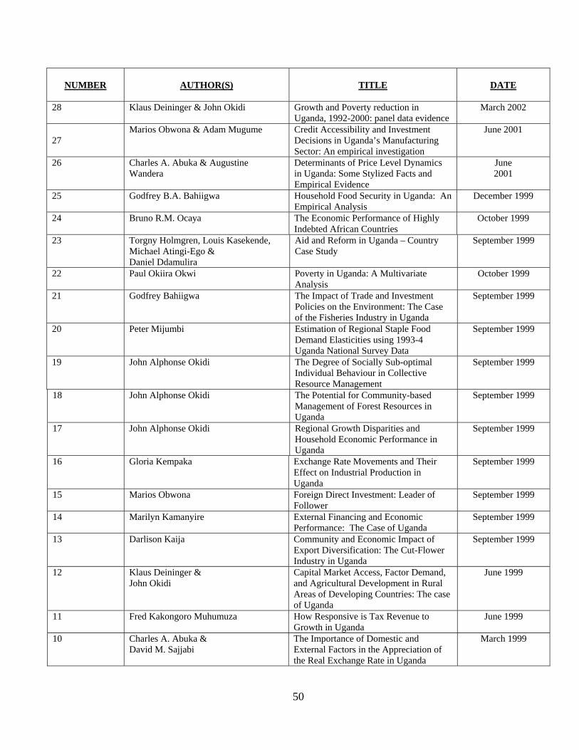
50
NUMBER
AUTHOR(S)
TITLE
DATE
28 Klaus Deininger & John Okidi Growth and Poverty reduction in Uganda, 1992-2000: panel data evidence
March 2002
27
Marios Obwona & Adam Mugume Credit Accessibility and Investment Decisions in Uganda’s Manufacturing Sector: An empirical investigation
June 2001
26 Charles A. Abuka & Augustine Wandera
Determinants of Price Level Dynamics in Uganda: Some Stylized Facts and Empirical Evidence
June 2001
25 Godfrey B.A. Bahiigwa Household Food Security in Uganda: An Empirical Analysis
December 1999
24 Bruno R.M. Ocaya The Economic Performance of Highly Indebted African Countries
October 1999
23 Torgny Holmgren, Louis Kasekende, Michael Atingi-Ego & Daniel Ddamulira
Aid and Reform in Uganda – Country Case Study
September 1999
22 Paul Okiira Okwi Poverty in Uganda: A Multivariate Analysis
October 1999
21 Godfrey Bahiigwa The Impact of Trade and Investment Policies on the Environment: The Case of the Fisheries Industry in Uganda
September 1999
20 Peter Mijumbi Estimation of Regional Staple Food Demand Elasticities using 1993-4 Uganda National Survey Data
September 1999
19 John Alphonse Okidi The Degree of Socially Sub-optimal Individual Behaviour in Collective Resource Management
September 1999
18 John Alphonse Okidi The Potential for Community-based Management of Forest Resources in Uganda
September 1999
17 John Alphonse Okidi Regional Growth Disparities and Household Economic Performance in Uganda
September 1999
16 Gloria Kempaka Exchange Rate Movements and Their Effect on Industrial Production in Uganda
September 1999
15 Marios Obwona Foreign Direct Investment: Leader of Follower
September 1999
14 Marilyn Kamanyire External Financing and Economic Performance: The Case of Uganda
September 1999
13 Darlison Kaija Community and Economic Impact of Export Diversification: The Cut-Flower Industry in Uganda
September 1999
12 Klaus Deininger & John Okidi
Capital Market Access, Factor Demand, and Agricultural Development in Rural Areas of Developing Countries: The case of Uganda
June 1999
11 Fred Kakongoro Muhumuza How Responsive is Tax Revenue to Growth in Uganda
June 1999
10 Charles A. Abuka & David M. Sajjabi
The Importance of Domestic and External Factors in the Appreciation of the Real Exchange Rate in Uganda
March 1999
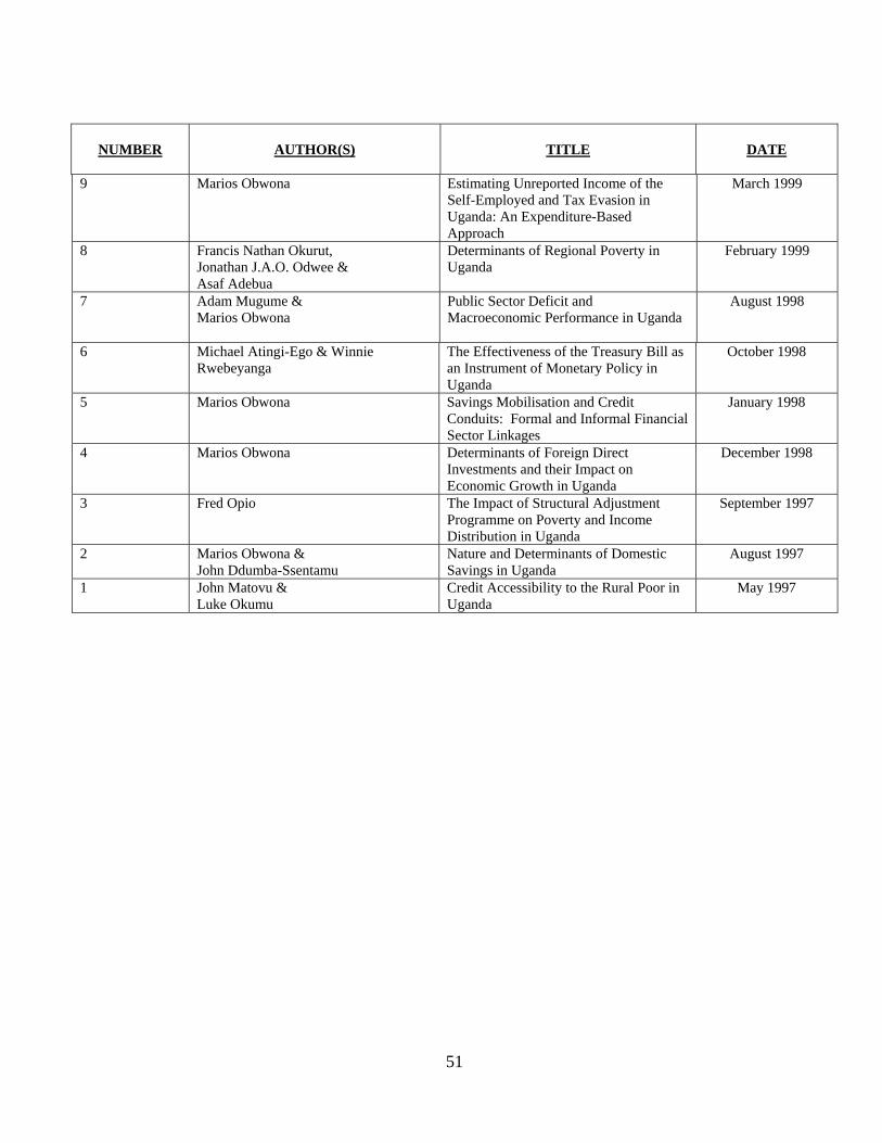
51
NUMBER
AUTHOR(S)
TITLE
DATE
9 Marios Obwona Estimating Unreported Income of the Self-Employed and Tax Evasion in Uganda: An Expenditure-Based Approach
March 1999
8 Francis Nathan Okurut, Jonathan J.A.O. Odwee & Asaf Adebua
Determinants of Regional Poverty in Uganda
February 1999
7 Adam Mugume & Marios Obwona
Public Sector Deficit and Macroeconomic Performance in Uganda
August 1998
6 Michael Atingi-Ego & Winnie Rwebeyanga
The Effectiveness of the Treasury Bill as an Instrument of Monetary Policy in Uganda
October 1998
5 Marios Obwona Savings Mobilisation and Credit Conduits: Formal and Informal Financial Sector Linkages
January 1998
4 Marios Obwona Determinants of Foreign Direct Investments and their Impact on Economic Growth in Uganda
December 1998
3 Fred Opio The Impact of Structural Adjustment Programme on Poverty and Income Distribution in Uganda
September 1997
2 Marios Obwona & John Ddumba-Ssentamu
Nature and Determinants of Domestic Savings in Uganda
August 1997
1 John Matovu & Luke Okumu
Credit Accessibility to the Rural Poor in Uganda
May 1997

Economic Policy Research Centre (EPRC) 51 Pool Road Makerere University Campus P. O. Box 7841 Kampala, Uganda
Tel: 256-41-541023 Fax: 256-41-541022 Email: [email protected]
Related Documents