1 Macroeconomic and Political Uncertainty and Cross Sectional Return Dispersion around the World Candie Chang Massey University [email protected] Ben Jacobsen TIAS Business School [email protected] Lillian Zhu University of Edinburgh [email protected] This draft: November 2017 Abstract Cross sectional return dispersion seems a simple, good and real time indicator of uncertainty. Internationally, cross-sectional return dispersion correlates strongly with measures of macroeconomic and political uncertainty like, recessions, international political crises, country risk ratings, and uncertainty indices related to government policies. While we find that return dispersion and implied volatility are correlated, surprisingly only return dispersion relates to the cross section of returns. Both measures seem to capture different types of uncertainty. Return dispersion captures political uncertainty mostly, whereas implied volatility seems linked to economic uncertainty. We gratefully acknowledge helpful comments from Frans de Roon, Angelica Gonzalez, Ufuk Gucbilmez, Wayne Ferson, Scott Baker, and seminar participants at University of Edinburgh, Tilburg University TIAS school for Business and Society, and 2016 FMA Doctoral Student Consortium. Any errors remain our own.

Welcome message from author
This document is posted to help you gain knowledge. Please leave a comment to let me know what you think about it! Share it to your friends and learn new things together.
Transcript
1
Macroeconomic and Political Uncertainty and
Cross Sectional Return Dispersion around the World
Candie Chang
Massey University
Ben Jacobsen
TIAS Business School
Lillian Zhu
University of Edinburgh
This draft: November 2017
Abstract
Cross sectional return dispersion seems a simple, good and real time indicator of uncertainty.
Internationally, cross-sectional return dispersion correlates strongly with measures of
macroeconomic and political uncertainty like, recessions, international political crises, country
risk ratings, and uncertainty indices related to government policies. While we find that return
dispersion and implied volatility are correlated, surprisingly only return dispersion relates to
the cross section of returns. Both measures seem to capture different types of uncertainty.
Return dispersion captures political uncertainty mostly, whereas implied volatility seems
linked to economic uncertainty.
We gratefully acknowledge helpful comments from Frans de Roon, Angelica Gonzalez, Ufuk
Gucbilmez, Wayne Ferson, Scott Baker, and seminar participants at University of Edinburgh,
Tilburg University TIAS school for Business and Society, and 2016 FMA Doctoral Student
Consortium. Any errors remain our own.

2
Macroeconomic and Political Uncertainty and
Cross Sectional Return Dispersion around the World
Abstract
Cross sectional return dispersion seems a simple, good and real time indicator of uncertainty.
Internationally, cross-sectional return dispersion correlates strongly with measures of
macroeconomic and political uncertainty like, recessions, international political crises, country
risk ratings, and uncertainty indices related to government policies. While we find that return
dispersion and implied volatility are correlated, surprisingly only return dispersion relates to
the cross section of returns. Both measures seem to capture different types of uncertainty.
Return dispersion captures political uncertainty mostly, whereas implied volatility seems
linked to economic uncertainty.
JEL classification: G12, G15, E60
Key words: Return dispersion, business cycles, political risk, economic policy uncertainty,
stock returns.

3
1. Introduction
The recent financial crisis of 2008 has made it clear that investors and regulators lack a proper,
simple and easy measure to capture macroeconomic and political uncertainty, let alone that one
would be able to capture it in real-time. As a consequence, the number of papers trying to link
different volatility measures to uncertainty has been growing (see for instance Cesa-Bianchi,
Pesaran, Rebucci (2014) and the papers within).
Our goal is a simple one. Can we find a measure that might capture uncertainty and which
can also be easily calculated in real time? Preferably one that is simple to measure and simple
to understand and that would give investors, financial regulators and other stakeholders a feel
in real time for the level of uncertainty as perceived by financial markets. Of course, stock
return volatility itself does not qualify as this measure cannot be observed in real time.
Moreover, it suffers from more serious problems. As Diebold and Yilmaz (2008) put it “There
are few studies attempting to link underlying macroeconomic fundamentals to stock return
volatility, and the studies that do exist have been largely unsuccessful. P.4)” Implied volatility
might be another candidate as it is traded directly. However, it is only available in a limited
number of countries.1
The literature suggests that cross sectional return dispersion, which is the cross sectional
standard deviation of stock returns, might be able to fill this gap and fulfil a role as a proxy for
uncertainty. For instance, for US data return dispersion is associated with unemployment
(Loungani, Rush, & Tave, 1990), the business cycle (Loungani, Rush, & Tave, 1991), the state
of the aggregate economy (Gomes, Kogan, & Zhang, 2003), micro-economic uncertainty
(Bloom, 2009) and market volatility (Stivers, 2003). Apart from this empirical evidence it also
intuitively seems a good measure for uncertainty. When there is good (bad) macroeconomic
1 Of course one could extract implied volatilities from option prices but apart from arbitrary model choices this would make the interpretation much harder to understand.

4
news for the general economy all stocks will go up (down) together and thus, return dispersion
will be low. However, it will be high when the future is uncertain as some stocks may go up
while others go down.
To investigate the usefulness of cross sectional dispersion as a practically useful and simple,
real time measure of uncertainty we embark on a comprehensive endeavour using a large set
of international data to verify whether return dispersion correlates with a broad set of
alternative uncertainty proxies (which are hard to measure in real time). More specifically, we
link return dispersion at a monthly level to different aspects of uncertainty including (local and
international) business cycles, political crises, country risk, economic policy uncertainty,
general uncertainty measured by use of the word ‘uncertainty’ in the media and uncertainty
that relates to fiscal, regulatory and monetary policies. Our tests rely on monthly data as these
other measures are often at best available at the monthly level. However, cross sectional return
dispersion itself can of course be measured at much higher frequencies. We look at the
international evidence extending the existing literature, which focuses on the US market mostly.
The monthly return dispersion series use the 50 largest market capitalization stocks in 18
different countries. This focus on the fifty largest market capitalization stocks makes this
measure even simpler and gives similar results to measures which include all stocks. Moreover,
this allows for a long sample starting in 1986. Using the fifty largest stocks also assures that
the series can easily be constructed and replicated for practical purposes. Last but not least, it
is well-known (Lo & MacKinlay, 1990) that small stocks lag stocks of larger firms, hence
focusing on the largest fifty stocks prevents delayed trading effects of smaller stocks. In the
next step, we link return dispersion to the cross section of stock returns in each country, asking
the question whether stocks that are more sensitive to (changes in2) return dispersion offer
2 We measure changes as the residuals from an AR(1) process estimated for the levels.
5
higher returns. For a limited number of countries where direct implied volatility data are
available we compare both measures.
Overall, our results suggest that return dispersion seems to capture different kinds of
macroeconomic and political uncertainty well. Furthermore, return dispersion (either measured
in changes or levels) is strongly linked to the cross-sectional stock returns in all countries.
Stocks with higher sensitivities to return dispersion have higher average returns. We compare
our return dispersion measure with implied volatility and find both measures respond
differently to our proxies for different types of uncertainty. Return dispersion has a higher
correlation with political uncertainty whereas, implied volatility seems stronger related to
economic uncertainty. However, and somewhat surprisingly, we find no evidence that (levels
or changes in) implied volatility correlate with the cross section of stock returns.
In our empirical analysis, we focus on five aspects of macroeconomic uncertainty. First, we
test whether return dispersion captures local and global business cycles using the business cycle
data from Fushing, Chen, Berge, and Jordà (2010). Our results confirm that in 11 out of 18
countries return dispersion is significantly higher during local business cycles. Once we include
the global business cycle, results are stronger than for the local business cycle (even though on
average a local business cycle effect persists). Return dispersion is significantly higher during
global recessions in 13 countries. On average global recessions raises return dispersion with
almost 50% (compared to expansions, assuming no local recession) suggesting that
international uncertainty might be more important than local uncertainty. To the best of our
knowledge this a new finding.
Second, we test whether return dispersion captures international political instability
controlling for business cycle effects. According to the rare disaster risk literature (for instance
Barro (2006), Gabaix (2012), Rietz (1988), Wachter (2013)), stock market returns correlate
6
strongly with changes in international crisis risk. For instance, based on the well-known ICB
international crisis risk database, Berkman, Jacobsen, and Lee (2011) show that stock market
returns go down significantly at the start of perceived international crises. While stock market
returns may be lower when a crisis starts, this does not necessarily hold for return dispersion
as all stocks may go down together. However, ongoing crises may lead to higher uncertainty,
hence higher return dispersion. We test this hypothesis and find that international political
uncertainty is an important contributing factor to return dispersion. The evidence for crises
starts is indeed mixed (although significantly positive when we pool the data). However, return
dispersion is significantly higher during international political crises in all but one of the
countries we consider.
Third, if we are willing to assume that when uncertainty is higher words like ‘uncertainty’
and ‘risk’ occur more frequently in Bloomberg articles, return dispersion is related to what may
be considered general uncertainty. Even though this may be a crude test, results suggest that
return dispersion is significantly positively related to the frequency of these words being used
in Bloomberg. After controlling for business cycles and international political crises effects
return dispersion is significantly higher in 11 out of 18 countries during month that the words
“uncertainty” and “risk” are used more frequently.
Forth, return dispersion seems linked to country risk based on the widely used International
Country Risk Guide (ICRG) data. This data set provides political, financial and economic risk
ratings. Again after controlling for the aforementioned factors, the composite ICRG rating (as
a proxy for each country’s business and investment status) increases return dispersion
significantly in many countries.
Fifth, we consider uncertainty that relates to fiscal, regulatory and monetary policies which
have large impact on employment, productivity and firm level investment (Bloom, 2009).

7
Baker, Bloom, and Davis (2016) construct an US economic policy uncertainty index which is
computed by counting the number of articles with policy related keywords in the leading
newspapers. They further developed a global economic policy uncertainty index and several
indices for other countries. We test if return dispersion is associated with both local and global
economic policy uncertainty. Cross sectional return dispersion increases significantly during
periods with high local economic policy uncertainty in Australia, Italy, Japan and US but not
in France, Germany, Ireland, Netherlands, Spain and Sweden. Global economic policy
uncertainty has strong and positive effect on return dispersion in seven out of eleven countries.
However, economic policy uncertainty has relatively small effect on return dispersion as ten
percent increase in uncertainty only raise return dispersion up around 30 basis points on
average.3
As return dispersion seems to capture different aspect of international uncertainty, return
dispersion might be able to explain the cross-section of stock returns. If so, stocks that are more
sensitive to return dispersion should offer higher returns. Jiang (2010) builds a model that
includes return dispersion directly in the pricing kernel. Chichernea, Holder, and Petkevich
(2015) use Jiang’s (2010) model to test the relation between return dispersion and the cross-
sectional expected returns. Following those two papers and extending their US evidence,
results indicate a strong positive relation between high sensitive return dispersion stocks and
stock returns in 18 countries, regardless whether we look at levels or changes in dispersion.
The difference between stocks with the high sensitivity to return dispersion and the portfolios
with low sensitivity to return dispersion is substantial (around 5% on average a month
3 We also employ several economic forecast variables as proxies of uncertainty in the US. We find that the forecast dispersion of personal consumption expenditure, real non-residential investment growth, term spread and AAA ranked government bond yield are significantly and positively related to return dispersion. The forecast dispersion of personal consumption expenditure for current quarter accounts for more than one third of the variation in return dispersion. As we only have the economic forecast dispersion for the US market (data from the survey of professional forecasters provided by the Federal Reserve Bank of Philadelphia), we do not include those results in our main findings.

8
regardless whether we control for sensitivity to the market and other factors or not). This holds
for all 18 countries. Results are also highly significant with an average t-value for the difference
between the high-return dispersion portfolios minus the low return dispersion portfolios of
10.69, controlling for four risk factors (market, size, value and momentum). These t-values
suggest that return dispersion easily passes the thresholds to account for datamining recently
suggested by Harvey, Liu, and Zhu (2014).4
Finally, we compare return dispersion with the implied volatility in seven countries for
which implied volatility data are available. Implied volatility is comparable to return dispersion
as this measure can also be observed in real time and at any frequency unlike many other risk
measures and has also been considered in the literature (for instance, Beber and Brandt (2009)
and Baker et al. (2016)). Our results show that implied volatility alone also captures uncertainty
associated with business cycles, political crises, general market uncertainty, country risk, and
economic policy. However, both measures respond differently to these uncertainty measures.
Return dispersion tends to respond strongly to measures of global business cycles and world
crisis risk. It does so even after controlling for implied volatility. Implied volatility significantly
captures the global economic policy uncertainty in all six countries (for which we have
economic policy and implied volatility data) but return dispersion does not.
We feel this paper makes the following contributions to the existing literature. First, we add
international evidence in 18 countries (to the US only evidence) that cross sectional return
dispersion correlates strongly with (new) measures of general, macro and political proxies of
uncertainty. It is important to focus on the international evidence particularly for global
macroeconomic and international political uncertainty as the United States might be a special
case. It is the world the largest economy and also a military superpower which has only rarely
4 They argue that many previously documented factors may not pass statistical significance tests once we take data mining into account and that we should use t-values cut-offs of 3 or higher.

9
seen battle in its own territory. Hence, when it comes to measuring uncertainty results for the
US may not necessarily be representative internationally. Second, we link return dispersion to
all sorts of proxies of macroeconomic and political uncertainty that have not been considered
before. Establishing a link between the international political crisis and return dispersion,
provides empirical support for theoretical models that allow for time-varying rare disaster risk
(Barro, 2006; Gabaix, 2012; Rietz, 1988; Wachter, 2013). The evidence indicates that cross
sectional return dispersion differs from implied volatility as it captures political uncertainty
better. Implied volatility seems to perform better capturing economic uncertainty. Third, we
also extent the US evidence cross sectional evidence and find that cross sectional return
dispersion (both levels and changes) correlate with the cross section of returns internationally
whereas implied volatility (both levels and changes) does not. And fourth, our international
evidence indicates that cross sectional return dispersion (based on even a limited number of 50
stocks) may for each country be a practically useful, simple and real time proxy to gauge
uncertainty.
These results are consistent with previous findings in the literature. The US evidence
suggests that during local recessions when uncertainty seems higher, also return dispersion
tends to be higher than during local expansions (Loungani et al., 1990). This study adds
international evidence on the relation between the local and the international business cycle
and return dispersion in individual countries. Return dispersion is also internationally linked to
the cross section of stock returns. Chichernea et al. (2015) illustrate for the US that return
dispersion largely explains the excess returns to accrual and investment hedge portfolios in US
stock market. Jiang (2010) considers US return dispersion as a priced factor and find it captures
differences in the cross sectional returns better than other well-known factors like momentum,
size and value. The international evidence here supports this finding. There are a number of
studies which compare return dispersion to conventional volatility measures. For instance,

10
Cesa-Bianchi, Pesaran, and Rebucci (2014) find that their results for global dispersion
measures are highly correlated with their realized volatility measure. Stivers (2003) provides
evidence that return dispersion is positively linked to future market-level volatility in US.
However, little evidence consists whether return dispersion and implied volatility are related
to the proxies we use for macroeconomic and political uncertainties.
2. A short literature review
The financial crisis during 2007-2008 period and its subsequent prolonged recovery brings the
topic of macroeconomic uncertainty back to the table. The literature suggests several proxies
of uncertainty and among these, volatility is the most popular one. However, Gorman, Sapra,
and Weigand (2010) suggest that the cross-sectional variation of equity returns may be a more
relevant way to measure risk rather than time-series volatility. Jiang (2010) finds that return
dispersion can be considered to be a macro state variable which can be used to capture the risk
contained in both business cycle fluctuations and macroeconomic restructuring.
2.1 Measuring macroeconomic uncertainty
Knight (1921) distinguishes uncertainty from risk and defines uncertainty as a situation of not
having ability to forecast the existing or future outcomes. The literature provides ample
evidence of the negative effects that policy uncertainty has on an economy. For instance,
economic policy uncertainty affects stock prices (Pastor & Veronesi, 2012), economic
activities (Baker, Bloom, & Davis, 2013), consumption and investment expenditures
(Alexopoulos & Cohen, 2009). Bloom, Floetotto, Jaimovich, Saporta-Eksten, and Terry (2012)
find that uncertainty is strongly countercyclical at both the aggregate and the industry-level.
They find that uncertainty is an essential factor in driving business cycles.
11
Therefore, it is important to measure uncertainty. Stock market volatility is a traditional
measure that is commonly used. However, in a recent work, Cesa-Bianchi et al. (2014) explore
the role of volatility on measuring economic uncertainty over 33 countries. They find that
volatility significantly leads business cycles. However, volatility has no or little direct effect
on real GDP. They suggest that volatility might be more a result rather than a cause of economic
uncertainty.
Baker et al. (2016) develop a relatively new measure of economic policy uncertainty (EPU).
They count the frequency of articles that refer to economy uncertainty and use it to build a
news-based EPU index. Baker et al. (2016) test their EPU index and find that it captures policy
related economic uncertainty well over time. Other studies propose other proxies of EPU.
Baker and Bloom (2013) list five proxies for uncertainty including stock index volatility, the
cross-firm stock returns spread, bond yields volatility, exchange rate volatility and GDP
forecast disagreement. Bali and Zhou (2016) consider the market variance risk premium (VRP)
as a proxy for economic uncertainty. They find that the variance risk premium is strongly
correlated with all the other sets of proxies including conditional variance of US output growth,
the conditional variance of Chicago Fed National Activity Index (CFNAI), extreme downside
risk in time-series and in cross-sectional financial firms’ returns, the credit default swap (CDS)
index, and the aggregate measure of investors’ disagreement. Additionally, Wang, Zhang, Diao,
and Wu (2015) use the changes in 23 commodity prices to predict EPU. Bekaert, Engstrom,
and Xing (2009) measure economic uncertainty by the conditional volatility of dividend growth.
Last but not least, Jurado, Ludvigson, and Ng (2013) suggest several indicators of uncertainty
including volatility of market returns (both implied and realized), cross sectional dispersion of
firm profits, returns, productivity and subjective (survey-based) forecast, and the appearance
of uncertainty-related key words in news publications.
12
2.2 Return dispersion
In the literature there is an increasing focus on the cross sectional return dispersion as a measure
of uncertainty. Theoretically, Christie and Huang (1995) find that, return dispersion will
increase during market stress according to the rational asset pricing models, as individual assets
have different sensitivities to market returns. In the US market they find that return dispersion
is higher during periods of large return changes. Recently, Angelidis, Sakkas, and Tessaromatis
(2015) show that return dispersion is able to predict the business cycles, business conditions
and unemployment rates. A higher world dispersion over the last three months indicates a
higher probability that the economy is currently in recession.
The literature suggests that return dispersion is closely linked to macroeconomic
uncertainty. Loungani et al. (1990) find that return dispersion predicts high unemployment
rates. A higher cross-industry dispersion in stock price growth leads to higher unemployment.
This evidence conforms to the sectoral shifts hypothesis that higher dispersion of inter-sectoral
shifts leads to higher unemployment by raising the required labour reallocation. Gomes et al.
(2003) and Zhang (2005) formally establish the theoretical link between return dispersion and
the state of the aggregate economy. Gomes et al. (2003) present a general equilibrium model
where the conditional capital asset pricing model holds, where firm betas vary with the market
state, and where firm betas are related to a firm’s size and book-to-market ratio. Given that
firm betas cannot be measured perfectly in practice, a firm’s size and book-to-market ratio are
likely to contain incremental information about the cross-sectional variation in mean returns,
their model suggests that return dispersion may contain incremental information about the
current state of the economy, beyond market-level returns. Zhang (2005) extends Gomes,
Kogan & Zhang’s (2003) framework and features costly reversibility of capital investment, the
countercyclical price of risk, and variation in the level of growth options across firms. His
framework predicts that some seemingly idiosyncratic risk variables, for example, the average
13
stock return variance, can affect firm-level systematic risk and expected returns because they
can be used in predicting the future evolution of the output price. Zhang (2005) suggests that
the market’s cross-sectional stock return volatility may be positively related to the future
industry cost of capital, based on simulation data.
Empirically, Loungani et al. (1991) find that return dispersion is associated with the
business cycle. Jiang (2010) illustrates that time-varying return dispersion is able to capture
economic restructuring, uncertainty shocks and business cycles. Jiang (2010) shows that
periods during major technology shocks result in extremely high return dispersion. Grobys and
Kolari (2015) use return dispersion to test whether changes in economic states would influence
asset pricing anomalies. Bali and Zhou (2016) find that price uncertainty explains the cross-
sectional variations in stock returns. Last but not least, Bekaert and Harvey (2000) use return
dispersion as a control variable for stock market integration. They suggest that when an
economy becomes more developed, reliance on particular sectors would decrease and thus,
increase cross sectional return dispersion.
2.3 Return dispersion and the cross section of returns
Jiang (2010) considers return dispersion as a risk factor that plays an essential role in capturing
the cross-sectional variation in expected returns. Stocks which are more sensitive to return
dispersion tend to have higher returns. Demirer and Jategaonkar (2013) expand Jiang’s (2010)
study and illustrate a systematic conditional relation between return dispersion and cross
section of stock returns. Generally speaking, the higher the sensitivity of a stock to return
dispersion, the higher its average return is. However, the premium on return dispersion
disappears when the market faces large losses. Chen, Demirer, and Jategaonkar (2015) extend
Jiang’s (2010) work and find similar evidence in the Chinese market. Chang, Cheng, and
Khorana (2000) examine the relationship between equity return dispersions and market returns
internationally. They find that the return dispersions increase linearly in the US, Japan and

14
Hong Kong when the prices move extremely high or low. However, in the South Korea and
Taiwan, they find smaller return dispersion during periods of extreme price movements. In this
paper, we extend international evidence to 18 countries and all of them suggesting that more
return dispersion sensitive stocks generate higher returns.
Return dispersion also seems related to asset pricing factors. Conrad and Kaul (1998) find
that the profitability of a momentum strategy can be attributed to return dispersion. Bhootra
(2011) confirms their result that return dispersion is a potential source of momentum profit.
Connolly and Stivers (2003) link return dispersion with return momentum and reversal. Weeks
with extremely high (low) dispersion are followed by a momentum (reversal) in weekly equity-
index returns. Stivers and Sun (2010) suggest that return dispersion is positively related to
subsequent value premiums and negatively related to subsequent momentum premiums. These
intertemporal relations remain strong even after controlling for a wide range of state variables
include the dividend yield, the default yield spread, the term yield spread and the short term
treasury yield. Kim (2012) expands their results and shows that return dispersion has predictive
power for the value premium in emerging countries but not in developed countries. Chichernea
et al. (2015) find that return dispersion provides a risk-based explanation to accrual and
investment anomalies. After 2008, low accrual and low-investment portfolios seem to get a
high risk premium as a compensation for the increased risk as measured by return dispersion.
2.4 Other risk measures
According to Jiang (2010) return dispersion relates to two dimensions of risk. One is related to
business cycles and the other is related to fundamental economic restructuring. Return
dispersion seems to be a better risk factor than time-series volatility (Gorman et al., 2010) and
the book-to-market factor (Jiang, 2010). Stivers (2003) and Connolly and Stivers (2006) show
that return dispersion conveys information about future volatility and Stivers (2003) shows that
firm return dispersion is positively related to future market volatility in the US. Connolly and
15
Stivers (2006) suggest that return dispersion is positively associated with both firm-level and
portfolio-level future return volatilities. Angelidis et al. (2015) find that return dispersion is a
good predictor of changes in market volatility. There is a positive and significant relation
between world return dispersion and world market volatility. Gomes et al. (2003) confirm their
results by showing that return dispersion has significant explanatory power for future aggregate
return volatility even after controlling for the market returns.
Return dispersion is also related to idiosyncratic volatility. For instance, Garcia, Mantilla-
Garcia, and Martellini (2014) use the cross-sectional variation of stock returns as a measure of
aggregate idiosyncratic volatility. Garcia et al. (2014) suggest that return dispersion is a
consistent and asymptotically efficient proxy for idiosyncratic volatility. Bali, Cakici, and Levy
(2008) use the difference between the variance of non-diversified portfolios and the variance
of the fully diversified portfolios as the average idiosyncratic volatility. They further
decompose total risk into firm, industry and market variance. Additionally, de Silva, Sapra,
and Thorley (2001) indicate that return dispersion is a function of stocks’ cross-sectional
variation and their sensitivity to market changes and the general level of idiosyncratic volatility.
3. Data
We obtain our return data from Compustat Global for all countries except for the US where we
use Center for Research in Security Prices (CRSP) stock return files. As noted before return
dispersion is simply the cross sectional standard deviation of stock returns:
𝑅𝐷𝑡 = √1
𝑁−1∑ (𝑅𝑖,𝑡 − 𝑅𝑀,𝑡)2𝑛
𝑖=1 (1)
where 𝑅𝐷𝑡 is the return dispersion at time t, N is the number of stocks included, 𝑅𝑖,𝑡 is the
return of individual stock i at time t, and 𝑅𝑀,𝑡 is the mean return of those N stocks at time t.
16
We prefer long series and preferably many countries but need to restrict our attention to
countries for which we can find reliable business cycle data and can create long enough
dispersion series. We use the international business cycle data derived by Fushing et al. (2010).
An advantage is that their methodology also allows for the creation of a global business cycle
so we can test whether the source of uncertainty may be global or local. As a result, the data
period for all the countries starts from January 1986 to December 2013 (when the most recent
ICB data end).
These criteria lead to return dispersions and business cycles jointly for 18 countries:
Australia, Austria, Belgium, Denmark, Finland, France, Germany, Ireland, Italy, Japan,
Netherlands, Norway, New Zealand, Spain, Sweden, Switzerland, the United Kingdom and the
United States. For some countries, long series are possible based on the constituents of the
main indices in those countries and we use these as a robustness test in our analysis (We report
those results in the Appendix C) This set consists of market indices for seven countries:
Australia, Finland, France, Germany, Japan, Switzerland and the United States. These time
series have at least 300 return dispersion observations based on all constituents of the main
indices in these countries. We consider returns at a monthly frequency as these tend to be less
noisy than high frequency data and many of our other variables are only available at monthly
frequency but return dispersion can of course be measured at much higher frequencies.
The first thing we want to establish is whether the return dispersion of the 50 largest (market
capitalization) stocks might be a good proxy for the more general market. Table 1 compares
the basic characteristics for the full market return dispersion and return dispersion of the 50
largest firms. The last column contains the correlations between these two measures in each
country. Generally, correlations tend to be very high ranging from 0.56 to 0.98. (We do not
have a full return dispersion index for Ireland). Using the US stock market as an example figure
1 shows that cross sectional return dispersion of all available stocks and cross sectional return
17
dispersion of the top 50 stocks are closely linked. They peak at almost the same time all the
way through with only a difference in magnitude. Unfortunately, it is hard to say which one
would be the most accurate measure. As noted in the introduction, it is well-known (Lo &
MacKinlay, 1990) that small stocks lag stocks of larger firms. If the full market is made up of
a large number of stocks this may cause return dispersion of the full index to respond with a
delay and essentially introduce noise. Still, differences are small and we focus on the return
dispersion (𝑅𝐷𝑡) of 50 largest firms (N=50) in every country.5 The advantage is that these series
are relatively easy to replicate. This is not only useful from an academic point of view but
might also make its use easier for practitioners to implement these measures. Hence from now
on the analysis focuses on the cross-sectional return dispersion measure for the 50 largest
stocks.
Please insert Table 1 around here
Please insert Figure 1 around here
For the return dispersion of 50 largest stocks the mean values of the return dispersion series
range from 5.68 percent to 10.61 percent and the median values are a bit lower from 5.12
percent to 9.21 percent. The US market has the lowest mean and median return dispersion. All
the distributions show positive skewness and are leptokurtic. We reject the null hypothesis that
return dispersion series follow normal distribution for all countries.
5 Connolly and Stivers (2003) also use large-firm portfolio (largest size-based decile portfolio) in calculating return dispersion as small firms add disruption because of high idiosyncratic volatility.

18
4. Return dispersion and macro economy
As a first eyeball test whether return dispersion is linked to macroeconomic uncertainty Figure
2 plots the monthly return dispersion of the US largest 50 stocks from January 1986 to
December 2013. The graph shows how return dispersion increases during periods of
macroeconomic news shocks, political events and stock market downturns. The shaded periods
are NBER recessions. The US return dispersion spikes during major events such as Gulf Wars,
Russian financial crisis, Dot-com Bubble, Bush Election 9/11, Lehman brother bankruptcy and
the following crisis of 2008 etc.
Please insert Figure 2 around here
4.1 Business cycles
Does return dispersion vary over the business cycle in all countries as in the US? If so, it should
be significantly higher during recessions. Based on the international business cycle data of
Fushing et al. (2010), we create dummy variables for both the country specific local business
cycle and the global business cycle (1= recession, 0 = expansion). We first regress our return
dispersion series on the country specific business cycle variable alone as shown in equation (2):
𝑅𝐷𝑡 = 𝛼 + 𝛽1𝐵𝐶_𝑙𝑜𝑐𝑎𝑙𝑡 + 𝜀𝑡 (2)
where 𝐵𝐶_𝑙𝑜𝑐𝑎𝑙𝑡 is the dummy variable for local business cycle (1= recession, 0 =
expansion). Then we include the global business cycle 𝐵𝐶_𝑔𝑙𝑜𝑏𝑎𝑙𝑡 as well in our second
regression (equation 3):
𝑅𝐷𝑡 = 𝛼 + 𝛽1𝐵𝐶_𝑙𝑜𝑐𝑎𝑙𝑡 + 𝛽2𝐵𝐶_𝑔𝑙𝑜𝑏𝑎𝑙𝑡 + 𝜀𝑡 (3)
For both regressions, the data end in September 2009 because the business cycle data end
in that month. Table 2 and 3 contain these results. Considering only the local business cycle,

19
the international evidence confirms to some extent the earlier US result that, the local business
cycle is indeed important. Generally, return dispersion is higher during recessions. In thirteen
out of our eighteen countries return dispersion is significantly higher during recessions.
However, many countries do not show as strong an effect as in the US where return dispersion
is on average fifty percent higher (9.35 percent versus 6.13 percent in expansions). Also, return
dispersion in Ireland, the Netherlands and Switzerland is more than 50 percent higher during
recessions. However, return dispersion in Japan is only 10 percent higher. On average we find
that for other countries, the difference is around 27 percent (9.74 percent versus 7.65 percent).
Please insert Table 2 around here
However, things change quite dramatically once return dispersion can fluctuate with the
global business cycle as well. Table 3 reports results for both local and global business cycles.
The local business cycle is still significant in 12 out of 18 countries but the size of the effect
halved compared to including the local business cycle only.
Given its significance level and the size of the coefficient. Return dispersion is significantly
higher (at the 10 percent level) during global recessions in 15 out of 18 countries. The size of
the effect is substantial. On average a global recession seems to raise the return dispersion with
almost 50% (11.05 percent versus 7.52 percent in expansions, assuming no local recession)
and the effect of return dispersion is 16 percent higher on average in a local recession (8.69
percent versus 7.52 percent in expansions assuming no global recession). Interestingly, these
results also hold for the US. Return dispersion in the US seems to depend more on global
economic conditions than economic conditions in the US only. In fact, once we control for
global recessions, the US is one of the countries where local effects become insignificant. Of
course part of this is caused because of the high correlations between some local country

20
recessions and the global recession dummy (correlations range from -0.01 for New Zealand to
0.82 for the US (we report the correlations of variables in Appendix A1)). The higher return
dispersion is associated with the global dummy rather than the local dummy in almost all
regressions. Pooling the data and estimate it either as a seemingly unrelated regression or as a
system gives similar results. The local business cycle is significant but the global factor seems
to weigh more heavily.
Please insert Table 3 around here.
4.2 International political crises
Would return dispersion also be affected by international political uncertainty? According to
the recent literature on rare disaster risk it should be. This literature introduced by Rietz (1988)
and made popular by Barro (2006) suggests that rare disaster risk may be an important factor
driving the equity premium. Indeed recent empirical evidence by Berkman et al. (2011)
suggests that the changes in the likelihood of international political crises have a strong impact
on stock market returns. They find that stock market returns go down significantly at the start
of perceived international crises based on the well-known ICB international crisis risk database.
While return dispersion does not necessarily increase when a crisis starts (all stocks may go
down together), it seems likely that ongoing international political crises raise uncertainty
which may only go down when when crises end. Although the end of crises effects might be
less clear as 1) the end of a crisis in the ICB database may be easier to anticipate, and 2) while
the end of crisis may reduce uncertainty it might also fuel uncertainty about the future.
We test this hypothesis using the international crises variables introduced by Berkman et
al. (2011), which we extend to December 2013. In line with their approach, we use the variables
that denote the number of crises starting in a month (start), ongoing crises in a month (during)
21
and a variable indicating the number of crises ending (end). We also use their World Crisis
Index (also constructed from the ICB database) which takes into account crisis severity, with
more serious crises getting a stronger weight.6 This may be a better proxy for actual perceived
crisis risk. (We report the results where we just rely on the number of crises in the appendix
A2). Table 4 presents the descriptive statistics of the world crises variables and world crises
index (WCI). The data range from January 1986 to December 2013. The number of ongoing
crisis is 1.46 a month on average. The means of the world crisis index start, during and end are
1.02, 4.81 and 1.04.
Please insert Table 4 around here
We control the effect of both local and global business cycle and add three variables to
equation (3) The first variable measures the WCI of crises starting in that month, (𝑆𝑡𝑎𝑟𝑡_𝑊𝐶𝐼𝑡)
the second one the WCI for ongoing crises during month t (𝐷𝑢𝑟𝑖𝑛𝑔_𝑊𝐶𝐼𝑡) and the last
variable the WCI of crises ending in month t (𝐸𝑛𝑑_𝑊𝐶𝐼𝑡).
𝑅𝐷𝑡 = 𝛼 + 𝛽1𝐵𝐶_𝑙𝑜𝑐𝑎𝑙𝑡 + 𝛽2𝐵𝐶_𝑔𝑙𝑜𝑏𝑎𝑙𝑡 + 𝛽3𝑆𝑡𝑎𝑟𝑡_𝑊𝐶𝐼𝑡 + 𝛽4𝐷𝑢𝑟𝑖𝑛𝑔_𝑊𝐶𝐼𝑡
+ 𝛽5𝐸𝑛𝑑_𝑊𝐶𝐼𝑡 + 𝜀𝑡 (4)
Table 5 shows the estimation results for international political crises. Return dispersion is
higher during times of crises. In all but one country the effect is significant. The crisis index
has a mean of 4.81 per month. This means that on average during international political crises
return dispersion is around 10 percent higher. There also seems to be a start of a crisis effect
although less strong (significant in six out of the 18 countries). If we pool the data in a system,
6 The world crises index sums up six dummy variables that capture six dimensions of the severity of a crisis. Each dummy variable equals 1 if the crisis started with violence, if violence is used during the crisis, if it is a full-scale war, if there is severe value threat, if the crisis is part of a protracted conflict, and if superpower is involved in the crisis. The WCI index ranges from zero to six.
22
the overall effect also indicates significance. Crises starts add another two percent to return
dispersion. The end of crises does not seem to add significantly to return dispersion.
Please insert Table 5 around here
4.3 Uncertainty around the world
In order to cover more general uncertainty, we consider another proxy. We assume that the
word ‘risk’ and ‘uncertainty’ will occur more frequently in months with higher perceived risk
and uncertainty in general. If so, then there is a simple test whether return dispersion captures
general uncertainty. This has the advantage that we can use it for all 18 countries. We count
the number of Bloomberg reports in every month that contains these two words and add in turn
one of these two variables to our regressions. In both cases we take the log as the number of
news articles seems to have grown exponentially over time. We use this word count uncertainty
as an explanatory variable with the control variable of business cycles and world crisis index
as below:
𝑅𝐷𝑡 = 𝛼 + 𝛽1𝐵𝐶_𝑙𝑜𝑐𝑎𝑙𝑡 + 𝛽2𝐵𝐶_𝑔𝑙𝑜𝑏𝑎𝑙𝑡 + 𝛽3𝑆𝑡𝑎𝑟𝑡_𝑊𝐶𝐼𝑡 + 𝛽4𝐷𝑢𝑟𝑖𝑛𝑔_𝑊𝐶𝐼𝑡
+ 𝛽5𝐸𝑛𝑑_𝑊𝐶𝐼𝑡 + 𝛽6𝑊𝑜𝑟𝑑𝐶𝑜𝑢𝑛𝑡𝑡 + 𝜀𝑡 (5)
Table 6 contains our results for the word ‘Uncertainty’ (as results are similar for the word
“risk” these are in the Appendix A3). Particularly for the US results are with a t-value of over
7 highly significant and of the expected sign. In months when the use of the word ‘uncertainty’
is high, return dispersion tends to dramatically increase. The explanatory power measured by
the R2 almost doubles to 40%. Maybe not surprising because Bloomberg originates from the
US. In many other countries, we find a positive significant effect as well, with the exception of
Australia, New Zealand and Spain where, the word count for uncertainty seems significantly

23
negative. Overall the effect is however significantly positive. The uncertainty effect is
positively significant in 11 out of 18 countries.
Please insert Table 6 around here
4.4 International country risk
We further include the International Country Risk Guide (ICRG) risk ratings as a proxy for
country-level uncertainty. ICRG provides rating regarding country’s political, economic and
financial risk every month. We use the Composite Risk Rating which including twelve political
risk components, five financial risk components, and five economic risk components. The data
ranges from 65 to 96. We test if return dispersion captures the movement of country risk. We
add the ICRG composite risk index as an uncertainty measure as shown in equation (6):
𝑅𝐷𝑡 = 𝛼 + 𝛽1𝐵𝐶_𝑙𝑜𝑐𝑎𝑙𝑡 + 𝛽2𝐵𝐶_𝑔𝑙𝑜𝑏𝑎𝑙𝑡 + 𝛽3𝑆𝑡𝑎𝑟𝑡_𝑊𝐶𝐼𝑡 + 𝛽4𝐷𝑢𝑟𝑖𝑛𝑔_𝑊𝐶𝐼𝑡
+ 𝛽5𝐸𝑛𝑑_𝑊𝐶𝐼𝑡 + 𝛽6𝑊𝑜𝑟𝑑𝐶𝑜𝑢𝑛𝑡𝑡 + 𝛽7𝐶𝑜𝑢𝑛𝑡𝑟𝑦_𝑅𝑖𝑠𝑘𝑡 + 𝜀𝑡 (6)
Table 7 shows the regression results. The overall effect of individual country risk on return
dispersion seems to be negative. However, in France, the Netherlands, Switzerland, UK and
US, they exhibit significantly positive relation. Ten units increase in the US country risk (mean
value to maximum value) will increase its stock market return dispersion by 2.2 percent.
Please insert Table 7 around here.
4.5 Economic policy uncertainty
Policy-related uncertainties such as taxes, government spending, regulations, interest rate etc.
have played an essential role in slowing down the recovery of the great depression of 2007-
2009 (Baker et al., 2013). As return dispersion has been considered to be an economic state

24
variable (see for instance Angelidis et al. (2015)), it may reflect economic policy uncertainty.
To test this hypothesis, we employ the economic policy uncertainty (EPU) index developed by
Baker et al. (2013). This index relies on monthly counts of articles in leading newspapers that
references to the economic, uncertainty and policy.7 Baker et al. (2013) first establish their
index in the US and evaluate its impact on macro economy. They find that the EPU index
spikes around major political shocks including the Gulf Wars, 9/11, presidential elections,
financial crisis etc.
Baker et al. (2013) also construct and EPU index for eleven countries. We employ the EPU
index in seven countries (France, Germany, Italy, Japan, Spain, UK and US) which overlap
with our sample of countries. Additionally, we include their global EPU index date back to
January 1997. The global EPU index is a composite index reflecting 18 countries’ uncertainty.
These EPU indices have been used in several studies as proxy of economic policy uncertainty
(for instance, Pástor and Veronesi (2013), Wang et al. (2015), Antonakakis, Chatziantoniou,
and Filis (2013), Karnizova and Li (2014)). The data are from their website
(http://www.policyuncertainty.com/). France economic policy uncertainty fluctuated most
among all seven countries. The standard deviation of the EPU index in France is 72.55
compared to 32.82 for the US.
To test if return dispersion is influenced by macroeconomic policies, we again extend our
previous regression to include both (the log of) local economic policy for each country
(𝐸𝑃𝑈_𝑙𝑜𝑐𝑎𝑙𝑡) and (the log of) global economic policy uncertainty (equation 7).
7 Baker, Bloom, and Davis (2015) construct the economic policy uncertainty index based on three components in their early draft paper. The components include the media coverage of references to economic uncertainty and policy, the number of federal tax code provision set to expire, and the degree of disagreement among economic forecasters. But in their latest draft they only include the newspaper coverage frequency.

25
𝑅𝐷𝑡 = 𝛼 + 𝛽1𝐵𝐶_𝑙𝑜𝑐𝑎𝑙𝑡 + 𝛽2𝐵𝐶_𝑔𝑙𝑜𝑏𝑎𝑙𝑡 + 𝛽3𝑆𝑡𝑎𝑟𝑡_𝑊𝐶𝐼𝑡 + 𝛽4𝐷𝑢𝑟𝑖𝑛𝑔_𝑊𝐶𝐼𝑡
+ 𝛽5𝐸𝑛𝑑_𝑊𝐶𝐼𝑡 + 𝛽6𝑊𝑜𝑟𝑑𝐶𝑜𝑢𝑛𝑡𝑡 + 𝛽7𝐶𝑜𝑢𝑛𝑡𝑟𝑦_𝑅𝑖𝑠𝑘𝑡
+ 𝛽8ln (𝐸𝑃𝑈_𝑙𝑜𝑐𝑎𝑙)𝑡 +𝛽9ln (𝐸𝑃𝑈_𝑔𝑙𝑜𝑏𝑎𝑙)𝑡 + 𝜀𝑡 (7)
Table 8 shows the results. The overall effect of both country specific EPU and global EPU
on return dispersion is significant and positive. Return dispersion is statistically larger during
higher country specific economic policy uncertainty in Australia, Italy, Japan, and the US. The
effect is economically small. For instance, 10 percent increase in economic policy uncertainty
will raise return dispersion around 37 basis points in the US and 25 basis points in Japan. Global
EPU has larger effect than local one. Global economic policy uncertainty has significant effect
on return dispersion in eight out of eleven countries we tested. However, the effect in Australia
is negative and is insignificant in the US.
Please insert Table 8 around here.
5. Return dispersion and the cross section of returns
As return dispersion seems to capture uncertainty well, one can easily relate it to returns. We
consider whether returns of stocks depend on their sensitivity with respect to return dispersion.
Jiang (2010) documents that return dispersion is a priced factor in the US and stocks with
higher sensitivities to return dispersion have higher average returns. We consider not only
levels but also changes in cross sectional return dispersion. Results for changes are similar
(although not as strong as for the levels and we report these in the Appendix B). We provide
evidence for 13 international stock markets, Australia, Belgium, France, Germany, Italy, Japan,

26
the Netherlands, Norway, Spain, Sweden, Switzerland, the UK and the US.8 Our sample period
starts from January 1986 to March 2014. We exclude very small firms. For each market in each
year, we consider the 90% largest common stocks based on the market capitalization at the end
of the previous year.9 We also identify the largest 50 stocks by the same market capitalization
measure.
The first step is to estimate the sensitivity of individual stocks to return dispersion. For each
market for each month for each stock with more than 15 daily return observations, we run a
time-series regression. Specifically, we regress the daily stock return on the mean return of the
largest 50 stocks (as a proxy for the market-wide movement) and the return dispersion of the
largest 50 stocks:
𝑅𝑖,𝑡 = 𝛼𝑖 + 𝛽𝑖,𝑅𝑀𝑅𝐹𝑅𝑀𝑅𝐹𝑡 + 𝛽𝑖,𝑅𝐷𝑅𝐷𝑡 + 𝜀𝑖,𝑡 (8)
where 𝑅𝑖,𝑡 is the return of the individual stock at time t, 𝑅𝑀𝑅𝐹𝑡 is the mean return of the largest
50 stocks at time t and 𝑅𝐷𝑡 is the return dispersion of the largest 50 stocks at time t. The
estimated coefficient (𝛽𝑖,𝑅𝐷) is the estimated sensitivity of the stock with respect to cross
sectional return dispersion measures.
In the second step we form quintile portfolios based on this estimated coefficient 𝛽𝑖,𝑅𝐷. For
each market for each month, we sort all the stocks by the estimated 𝛽𝑖,𝑅𝐷. Portfolio 1 consists
of stocks with the smallest 20 percent 𝛽𝑖,𝑅𝐷 whereas Portfolio 5 consists of stocks with the
largest 20 percent 𝛽𝑖,𝑅𝐷.
8 We exclude five markets from this analysis because these markets have been small markets such that there are not enough observations in the early months for analysis. These five markets are Finland, Denmark, Austria, New Zealand and Ireland. 9 We only focus on stocks that are traded in the domestic currency, which usually accounts for more than 90% of all stocks.
27
In the third step we calculate monthly returns for these portfolios. For each market for each
month for each portfolio, we calculate the monthly value-weighted portfolio return using the
monthly return, of the same month as the portfolio formation month, of all individual stocks
constituting the portfolio where the weighting is the market capitalization as of the end of the
previous month.
In our last step we consider whether stocks with higher sensitivities to return dispersion
have higher average returns. We present two sets of results, one is the average monthly CAPM
alphas and the other is the four-factor alphas. The CAPM alphas are returns after controlling
for the mean return of the largest 50 stocks (𝑅𝑀𝑅𝐹𝑡, as a proxy for the “market” factor). The
four-factor alphas are the returns after controlling for the Fama-French three factors (market,
size and value) and the momentum factor.
Table 9 reports the results for CAPM alphas and Table 10 reports the four-factor alphas.
We plot the CAPM alphas of the value weighted portfolios in Figure 3. Stock returns are
positively related to their sensitivity with respect to return dispersion. The returns increase
monotonically as their sensitivities increase, regardless whether we consider CAPM alphas or
four-factor alphas. For all the markets, the average alphas of the portfolios with the smallest
return dispersion sensitivities (Group 1) are negative except for the equal-weighted US stocks.
The mean returns of portfolios with the largest return dispersion sensitivities (Group 5) are
positive and also highly statistically significant. For the middle groups, there is at least one
group with a mean return that is statistically insignificantly different from zero: for raw returns,
it is usually Group 2; for CAPM alphas, it is usually Group 3. The differences in the mean
return between Group 5 and Group 1 range from 4.4% to 6.4% for the raw returns. For the
CAPM alphas, average differences range from 3.5% to 6.4%. Again t-values for these
differences indicate that the differences are highly significant. On average, we find a t-value of
around 9 for the raw returns and approximately a t-value of 15 for the CAPM alphas.

28
Please insert Table 9 around here
Please insert Table 10 around here
Please insert Figure 3 around here
In short, stocks that are more sensitive to return dispersion generate substantially higher
abnormal returns.10
6. Return dispersion and implied volatility
Implied volatility derived from an option contract is often used as a proxy for overall economic
uncertainty. It is a forward-looking volatility measure that contains information about expected
market fluctuations. In the G5 countries implied volatility is nowadays traded. The previous
literature shows a close link between the implied volatility and the economic uncertainty. For
instance, Beber and Brandt (2009) suggest that a high macroeconomic uncertainty period is
followed lower implied volatility. Also, Stivers (2003) finds that the dispersion in firm returns
10 In order to test whether these results are not caused by construction, we conduct the Monte Carlo simulation. We generate daily random samples, estimate monthly return series by cumulating the daily stimulations and repeat the process 100 times. The detailed procedure are as follows. First, we take the full sample market index to estimate market index sample mean and standard deviation. Use those characteristics of the original market index, we generate simulated market return series. We use the randomly generated market index as the return of the market portfolio. Second, we use the original individual stock returns regress on the original market index according to the CAPM model in order to estimate constant, beta, standard deviation of error term for each stock over the full sample. Then we generate individual stock return series using simulated market return series and the estimations from CAPM model. Third, we use the randomly generated market index as the return of the market portfolio. We construct return dispersion from the randomly generated stock returns of all individual stocks. Forth, we cumulate the daily returns to get the monthly data. We calculate the return dispersion using all individual stocks. Finally, we sort equal-weighted quintile portfolios every month based on stocks’ exposure to return dispersion as what we done using real data. The results of the simulated data are if anything go against those using the real dataset: the higher the exposure to return dispersion the lower return. This suggests that the methodology does not cause the effect we observe in the real data. These results are available on request from the authors.
29
provide incremental information about US market-level future volatility during period 1927 to
1995. We compare return dispersion with implied volatility. Just like return dispersion it is
easy to observe in at least the five countries for which these data are available.
6.1 Implied volatility and macroeconomic uncertainty
We first compare co-movements between implied volatility and return dispersion visually. We
obtain the implied volatility indices in G5 countries include CAC40 Volatility Index (France),
VDAX New Volatility Index (Germany), NIKKEI Stock Average Volatility Index (Japan),
FTSE 100 Volatility Index (UK) and CBOE SPX Volatility VIX (US). Figure 4 plots the return
dispersion series and implied volatility index for each country. Although these two measures
correlate, there still exists certain periods that they deviate from each other. For instance, during
the ten-year period of 1992 to 2002, return dispersion is extremely high while implied volatility
is around an average level.
Please insert Figure 4 around here
Table 11 reports the basic characteristics of the implied volatility. The implied volatility in
G5 countries indeed correlates with the corresponding countries’ return dispersion, but the
correlation is not high. The average correlation is less than 0.6 especially for Japan where the
correlation is only 0.32. The first-order autocorrelations, ρ(1) shows that a high implied
volatility this month increases the likelihood of a high implied volatility next month for all five
countries. As the first-order autocorrelations are relatively high, we further test if there exist
unit root by using Dicky-Fuller test. We reject the hypothesis of having a unit root for all series.
Please insert Table 11 around here

30
The next is whether implied volatility is also a risk measure for macroeconomic uncertainty.
Equation 9 shows the regression on business cycles, international political crisis, word count
uncertainty, country risk, and economic policy uncertainty, similar to return dispersion but now
the dependent variable is the implied volatility at month t (𝑉𝐼𝑋𝑡).:
𝑉𝐼𝑋𝑡 = 𝛼 + 𝛽1𝐵𝐶_𝑙𝑜𝑐𝑎𝑙𝑡 + 𝛽2𝐵𝐶_𝑔𝑙𝑜𝑏𝑎𝑙𝑡 + 𝛽3𝑆𝑡𝑎𝑟𝑡_𝑊𝐶𝐼𝑡 + 𝛽4𝐷𝑢𝑟𝑖𝑛𝑔_𝑊𝐶𝐼𝑡
+ 𝛽5𝐸𝑛𝑑_𝑊𝐶𝐼𝑡 + 𝛽6𝑊𝑜𝑟𝑑𝐶𝑜𝑢𝑛𝑡𝑡 + 𝛽7𝐶𝑜𝑢𝑛𝑡𝑟𝑦_𝑅𝑖𝑠𝑘𝑡
+ 𝛽8ln (𝐸𝑃𝑈_𝑙𝑜𝑐𝑎𝑙)𝑡 +𝛽9ln (𝐸𝑃𝑈_𝑔𝑙𝑜𝑏𝑎𝑙)𝑡 + 𝜀𝑡 (9)
Panel A of Table 12 has the regression results for G5 countries from January 2000 to
December 2013 and the pooled OLS (system) and seemingly unrelated regression (sur) that
considers these G5 countries as a system. Implied volatility seems to capture the uncertainty
associated with these variables well. Implied volatility series correlate with the global business
cycles but not local business cycles. The ongoing political crisis and country risk positively
affects implied volatility as well in all G5 countries. However, word count uncertainty has a
negative effect on implied volatility. Moreover, implied volatility series are significantly
affected by the global economic policy uncertainty but not the local one. For instance, 10%
increase in Global economic policy uncertainty will raise implied volatility by 2.4 units which
is around 10% of the average implied volatility level. In fact, results for implied volatility seems
stronger indicating that implied volatility is able to capture economic policy uncertainty better
than return dispersion.
Please insert Table 12 around here
31
For better comparison, Panel B of Table 12 contains the results for return dispersion during
the same period with G5 countries. Return dispersion is able to capture global business cycles,
ongoing political crisis, country risk, local economic policy uncertainty (for seemingly
unrelated regressions only), and global economic policy uncertainty as well.
6.2 Implied volatility and cross-sectional stock returns
As implied volatility does a good job in capturing macroeconomic uncertainties, a logical
question is whether or not the implied volatility also relates to the cross section of stock returns.
Similarly to section 5. We test whether stocks with higher sensitivities to implied volatility
produce higher average returns. (again we report levels and also consider changes (In Appendix
B), but the latter are similar to the level). We run the following time-series regression:
𝑅𝑖,𝑡 = 𝛼𝑖 + 𝛽𝑖,𝑅𝑀𝑅𝐹𝑅𝑀𝑅𝐹𝑡 + 𝛽𝑖,𝑣𝑖𝑥𝑉𝐼𝑋𝑡 + 𝜀𝑖,𝑡 (10)
where 𝑅𝑖,𝑡 is the individual firm return, 𝑅𝑀𝑅𝐹𝑡 is the equal-weighted average return of the
largest 50 firm and 𝑉𝐼𝑋𝑡 is the implied volatility. Every year we use the largest 90% market
capitalisation stocks (ranked at the end of the previous year). At the end of each month, we sort
stocks into quintile portfolios based on the value of implied volatility risk loadings over the
month. Panel A of Table 13 presents the average returns of the value-weighted portfolios and
Panel B reports the average returns of the equal-weighted portfolios. For all the portfolios, we
report the raw return, CAPM alphas and four-factor (market, size, value and momentum factors)
alphas. For most the countries, the difference between portfolios that are most sensitive to
implied volatility and portfolios that are least sensitive to implied volatility are statistically zero
except for the value-weighted portfolios in the UK and the US. For the US, the value-weighted
portfolio with stocks that have the highest sensitivity generates an average higher four-factor
alpha of 0.66 percent than portfolio with stocks that have the lowest sensitivity. For the UK,
the difference is 1.13 percent and statistically significant with a t-value of 2.52.
32
Please insert Table 13 around here
Please insert Figure 5 around here
The difference between Figure 3 and Figure 5 is striking. We have two proxies that seems
to measure both macroeconomic and political uncertainty. However, one (return dispersion)
shows a strong relation with the cross section of returns whereas the other shows no relation
whatsoever. We have done a number of tests but find no clear explanation what drives this
difference. We have not been able to explain it, other than the obvious conclusion which is
that the differences between the two measures is what they are and return dispersion captures
the uncertainty related to the cross section of returns whereas implied volatility does not.
6.3 A horserace between return dispersion and implied volatility
In order to see more explicitly whether return dispersion and implied volatility are linked with
certain types of uncertainty, we run a horse race between the two measures. We use each type
of uncertainty as the dependent variable and use both return dispersion (𝑅𝐷𝑡) and implied
volatility (𝐼𝑉𝑡) as explanatory variable (equation 11).
𝑈𝑛𝑐𝑒𝑟𝑡𝑎𝑖𝑛𝑡𝑦𝑡 = 𝛼 + 𝛽1𝑅𝐷𝑡 + 𝛽2𝐼𝑉𝑡 + 𝜀𝑡 (11)
where 𝑈𝑛𝑐𝑒𝑟𝑡𝑎𝑖𝑛𝑡𝑦𝑡 is the local business cycle dummy, global business cycle dummy, start
crises, ongoing crises, ending crises, word count uncertainty, international country risk, local
economic policy uncertainty, and global economic policy uncertainty in turn. Table 14 contains
our results for pooled OLS (system) and seemingly unrelated regressions (sur) on G5 countries.
The system results demonstrate that return dispersion and implied volatility are significantly
different. With regard to political risk (political crisis and country risk), return dispersion seems

33
to be more sensitive to this type of risk compared to implied volatility. With respect to the
uncertainty that computed by media coverage (word count uncertainty and economic policy
uncertainty), implied volatility does a better job than return dispersion. However, the seemingly
unrelated regressions indicate that return dispersion and implied volatility are only different in
capturing global business cycle and country risk. It is hard to distinguish them in terms of other
aspects of uncertainties.
Please insert Table 14 around here
Moreover, we test whether once we control for implied volatility, return dispersion is still
a measure of uncertainty. We add implied volatility as a control variable in equation (7). Panel
A of table 15 reports the results. The effect of return dispersion is reduced but not eliminated.
After controlling for implied volatility, return dispersion is higher during global recession,
political crisis and higher country risk period. The effect of economic policy uncertainty on
return dispersion is eliminated. We further test if implied volatility could capture those
uncertainties well with the control of return dispersion. Panel B of table 15 shows the regression
that using implied volatility as dependent variable. It seems that the effect of business cycles
on implied volatility is eliminated by return dispersion. In both tests, return dispersion is
strongly and positively associated with implied volatility.
Please insert Table 15 around here
7. Conclusion
The goal of this paper is a simple one. Can we find a measure that might capture uncertainty
and which can also be easily calculated in real time? Preferably one that is simple to measure
34
and simple to understand and that would give investors, financial regulators and other stake
holders a feel in real time for the level of uncertainty as perceived by financial markets.
Recent events and academic studies have highlighted the importance of measuring
macroeconomic and political uncertainty. Our goal is to find a measure that might capture
uncertainty and which can also be easily calculated in real time? Preferably one that is simple
to measure and simple to understand and that would give investors, financial regulators and
other stake holders a feel in real time for the level of uncertainty as perceived by financial
markets. This study links cross sectional return dispersion with different aspects of
uncertainties in 18 countries. We show that return dispersion is large during local and global
recessions, international political crisis, high economic policy uncertain periods and high
general market uncertain periods in most countries. Contrary to implied volatility cross
sectional return dispersion also seems strongly linked to the cross section of returns. It also
captures different aspect than implied volatility does, with a stronger link to political risk. All
in all, the evidence suggests that investors are able to gauge at least some of the uncertainty in
real time by closely monitoring cross sectional return dispersion. What we cannot explain is
why both implied volatility and cross sectional return dispersion seem both intuitively
appealing risk measures, and are correlated – although not to the extreme) one has a strong link
to the cross section of returns (cross sectional return dispersion) whereas the other (implied
volatility does not). We leave this as a puzzle to be explained.

35
References
Alexopoulos, M., & Cohen, J. (2009). Uncertain times, uncertain measures. University of Toronto
Department of Economics Working Paper, 352.
Angelidis, T., Sakkas, A., & Tessaromatis, N. (2015). Stock market dispersion, the business cycle
and expected factor returns. Journal of Banking & Finance, 59, 265-279.
Antonakakis, N., Chatziantoniou, I., & Filis, G. (2013). Dynamic co-movements of stock market
returns, implied volatility and policy uncertainty. Economics Letters, 120(1), 87-92.
Baker, S. R., & Bloom, N. (2013). Does uncertainty reduce growth? Using disasters as natural
experiments (No. w19475). National Bureau of Economic Research.
Baker, S. R., Bloom, N., & Davis, S. J. (2016). Measuring economic policy uncertainty. The
Quarterly Journal of Economics, 131(4), 1593-1636.
Bali, T. G., Cakici, N., & Levy, H. (2008). A model-independent measure of aggregate
idiosyncratic risk. Journal of Empirical Finance, 15(5), 878-896.
Bali, T. G., & Zhou, H. (2016). Risk, uncertainty, and expected returns. Journal of Financial and
Quantitative Analysis, 51(3), 707-735.
Barro, R. J. (2006). Rare disasters and asset markets in the twentieth century. The Quarterly
Journal of Economics, 121(3), 823-866.
Beber, A., & Brandt, M. W. (2008). Resolving macroeconomic uncertainty in stock and bond
markets. Review of Finance, 13(1), 1-45.
Bekaert, G., Engstrom, E., & Xing, Y. (2009). Risk, uncertainty, and asset prices. Journal of
Financial Economics, 91(1), 59-82.
Bekaert, G., & Harvey, C. R. (2000). Foreign speculators and emerging equity markets. The
Journal of Finance, 55(2), 565-613.
Berkman, H., Jacobsen, B., & Lee, J. B. (2011). Time-varying rare disaster risk and stock
returns. Journal of Financial Economics, 101(2), 313-332.
Bhootra, A. (2011). Are momentum profits driven by the cross-sectional dispersion in expected
stock returns?. Journal of Financial Markets, 14(3), 494-513.
Bloom, N. (2009). The impact of uncertainty shocks. econometrica, 77(3), 623-685.
Bloom, N., Floetotto, M., Jaimovich, N., Saporta-Eksten, I., & Terry, S. J. (2012). Really uncertain
business cycles (No. w18245). National Bureau of Economic Research.
Cesa-Bianchi, A., Pesaran, M. H., & Rebucci, A. (2014). Uncertainty and economic activity: A
global perspective.
Chang, E. C., Cheng, J. W., & Khorana, A. (2000). An examination of herd behavior in equity
markets: An international perspective. Journal of Banking & Finance, 24(10), 1651-1679.
Chen, C. D., Demirer, R., & Jategaonkar, S. P. (2015). Risk and return in the Chinese stock market:
Does equity return dispersion proxy risk?. Pacific-Basin Finance Journal, 33, 23-37.
Chichernea, D. C., Holder, A. D., & Petkevich, A. (2015). Does return dispersion explain the
accrual and investment anomalies?. Journal of Accounting and Economics, 60(1), 133-148.
36
Christie, W. G., & Huang, R. D. (1995). Following the pied piper: Do individual returns herd
around the market?. Financial Analysts Journal, 51(4), 31-37.
Connolly, R., & Stivers, C. (2003). Momentum and reversals in equity‐index returns during
periods of abnormal turnover and return dispersion. The Journal of Finance, 58(4), 1521-1556.
Connolly, R., & Stivers, C. (2006). Information content and other characteristics of the daily cross-
sectional dispersion in stock returns. Journal of Empirical Finance, 13(1), 79-112.
Conrad, J., & Kaul, G. (1998). An anatomy of trading strategies. The Review of Financial
Studies, 11(3), 489-519.
De Silva, H., Sapra, S., & Thorley, S. (2001). Return dispersion and active management. Financial
Analysts Journal, 57(5), 29-42.
Demirer, R., & Jategaonkar, S. P. (2013). The conditional relation between dispersion and
return. Review of Financial Economics, 22(3), 125-134.
Diebold, F. X., & Yilmaz, K. (2008). Macroeconomic volatility and stock market volatility,
worldwide (No. w14269). National Bureau of Economic Research.
Fushing, H., Chen, S.-C., Berge, T. J., & Jordà, Ò. (2010). A chronology of international business
cycles through non-parametric decoding.
Gabaix, X. (2012). Variable rare disasters: An exactly solved framework for ten puzzles in macro-
finance. The Quarterly journal of economics, 127(2), 645-700.
Garcia, R., Mantilla-Garcia, D., & Martellini, L. (2014). A model-free measure of aggregate
idiosyncratic volatility and the prediction of market returns. Journal of Financial and
Quantitative Analysis, 49(5-6), 1133-1165.
Gomes, J., Kogan, L., & Zhang, L. (2003). Equilibrium cross section of returns. Journal of
Political Economy, 111(4), 693-732.
Gorman, L. R., Sapra, S. G., & Weigand, R. A. (2010). The role of cross-sectional dispersion in
active portfolio management.
Grobys, K., & Kolari, J. W. (2015). Return dispersion and cross-sectional asset pricing anomalies.
In Proceedings of the 2015 Paris Financial Management Conference.
Harvey, C. R., Liu, Y., & Zhu, H. (2016). … and the cross-section of expected returns. The Review
of Financial Studies, 29(1), 5-68.
Jiang, X. (2010). Return dispersion and expected returns. Financial Markets and Portfolio
Management, 24(2), 107-135.
Jurado, K., Ludvigson, S. C., & Ng, S. (2015). Measuring uncertainty. The American Economic
Review, 105(3), 1177-1216.
Karnizova, L., & Li, J. C. (2014). Economic policy uncertainty, financial markets and probability
of US recessions. Economics Letters, 125(2), 261-265.
Kim, D. (2012). Value premium across countries. The Journal of Portfolio Management, 38(4),
75-86.
Knight, F. H. (2012). Risk, uncertainty and profit. Courier Corporation.

37
Lo, A. W., & MacKinlay, A. C. (1990). When are contrarian profits due to stock market
overreaction?. The Review of Financial Studies, 3(2), 175-205.
Loungani, P., Rush, M., & Tave, W. (1990). Stock market dispersion and unemployment. Journal
of Monetary Economics, 25(3), 367-388.
Loungani, P., Rush, M., & Tave, W. (1991). Stock market dispersion and business
cycles. Economic Persepctives, 15(4), 2-8.
Pastor, L., & Veronesi, P. (2012). Uncertainty about government policy and stock prices. The
Journal of Finance, 67(4), 1219-1264.
Pástor, Ľ., & Veronesi, P. (2013). Political uncertainty and risk premia. Journal of Financial
Economics, 110(3), 520-545.
Rietz, T. A. (1988). The equity risk premium a solution. Journal of monetary Economics, 22(1),
117-131.
Stivers, C., & Sun, L. (2010). Cross-sectional return dispersion and time variation in value and
momentum premiums. Journal of Financial and Quantitative Analysis, 45(4), 987-1014.
Stivers, C. T. (2003). Firm-level return dispersion and the future volatility of aggregate stock
market returns. Journal of Financial Markets, 6(3), 389-411.
Wachter, J. A. (2013). Can Time‐Varying Risk of Rare Disasters Explain Aggregate Stock Market
Volatility?. The Journal of Finance, 68(3), 987-1035.
Wang, Y., Zhang, B., Diao, X., & Wu, C. (2015). Commodity price changes and the predictability
of economic policy uncertainty. Economics Letters, 127, 39-42.
Zhang, L. (2005). The value premium. The Journal of Finance, 60(1), 67-103.

38
Table 1: Descriptive statistics
Table 1 reports the basic statistics (mean, median, max, min, standard deviation, skewness and kurtosis) of return dispersion made by 50 largest market capitalization
stocks (RD 50) and return dispersion of all stocks (RD all). The return dispersion is calculated as the cross-sectional standard deviation of stock returns at time t. Both
return dispersion series are computed from January 1986 to December 2013. We report the correlation between those two measures in the last column. The mean,
median, maximum and minimum values are in percentage.
Table 1: Basic statistics of return dispersion
Mean Median Max Min Std. Dev. Skewness Kurtosis Obs Correlation
between
RD50 and
RD all RD 50 RD all RD 50 RD all RD 50 RD all RD 50 RD all RD 50 RD all RD 50 RD all
RD
50
RD
all
RD
50
RD
all
Australia 7.16 11.39 6.27 10.79 30.10 32.22 1.96 5.27 0.03 0.03 3.51 1.76 19.80 8.93 336 300 0.56
Austria 8.57 7.94 7.78 7.01 33.53 28.18 2.25 3.33 0.04 0.04 2.34 2.20 11.56 9.73 336 253 0.65
Belgium 6.86 6.77 6.13 5.70 28.59 36.86 1.82 1.85 0.03 0.04 2.32 3.06 11.92 19.24 336 276 0.84
Denmark 8.14 7.80 7.30 6.77 41.11 26.66 3.93 2.99 0.04 0.04 3.54 2.15 25.05 9.37 336 290 0.76
Finland 8.92 8.50 8.07 7.64 27.70 56.37 3.15 1.63 0.03 0.05 1.51 4.05 6.68 33.48 336 308 0.81
France 6.80 6.77 6.11 6.12 20.21 19.15 1.44 2.64 0.03 0.03 1.86 1.88 8.29 7.73 336 312 0.93
Germany 6.97 6.48 6.16 5.73 26.48 28.46 1.40 2.69 0.03 0.03 2.21 2.43 10.75 12.80 336 305 0.91
Ireland 10.61 - 9.21 - 41.04 - 3.56 - 0.05 - 1.96 - 8.37 - 336 0 -
Italy 7.43 7.02 6.77 6.41 44.83 17.66 3.31 3.22 0.03 0.03 5.02 1.28 53.08 4.73 336 196 0.58
Japan 7.43 7.98 6.58 7.53 25.35 17.60 2.98 3.24 0.03 0.03 1.89 0.79 7.80 3.60 336 336 0.78
Netherlands 7.65 8.93 6.64 6.99 40.13 58.21 1.59 2.65 0.04 0.06 3.18 3.52 20.04 22.61 336 238 0.70
Norge 9.96 11.24 8.91 9.81 42.86 38.06 1.71 4.47 0.04 0.06 2.54 2.21 14.82 9.05 336 158 0.84
New
Zealand
9.10 6.73 7.91 6.09 32.80 20.67 2.60 3.55 0.04
0.03 2.09 2.32 9.37 10.85 336
126 0.83
Spain 7.85 7.23 6.84 6.39 65.08 26.84 1.43 2.71 0.05 0.03 6.31 1.85 73.13 9.33 336 300 0.72
Sweden 7.49 6.91 6.89 6.04 23.48 20.79 1.80 3.02 0.03 0.03 1.56 2.08 6.95 8.41 336 93 0.84
Switzerland 6.80 6.41 6.11 5.75 36.60 18.41 1.89 1.94 0.03 0.03 3.79 1.58 30.53 6.26 336 306 0.76
UK 6.66 7.47 5.84 6.33 21.00 19.73 1.34 4.06 0.03 0.03 1.84 2.03 7.26 7.36 336 67 0.98
US 5.68 8.59 5.12 7.72 24.57 22.85 2.09 4.79 0.02 0.03 2.56 1.70 13.86 6.37 336 330 0.79

39
Table 2: Return dispersion over local business cycles
Table 2 reports the results of the univariate regressions of 𝑅𝐷𝑡 = 𝛼 + 𝛽1𝐵𝐶_𝑙𝑜𝑐𝑎𝑙𝑡 + 𝜀𝑡 , where 𝑅𝐷𝑡 is the return dispersion of the largest 50 market
capitalization stocks at time t. Local BC is a dummy variable that equals one if the country is in recession and zero otherwise. System shows the results of
pooled OLS and Sur shows the results of seemingly unrelated regression. We use robust standard errors. Coefficients are in percentage.
constant t-value local BC t-value Adjusted R2
Australia 7.26 33.43 1.50 1.76 0.01
Austria 8.29 38.17 3.59 3.75 0.09
Belgium 6.59 34.16 1.06 1.72 0.01
Denmark 7.96 38.84 0.77 1.22 0.00
Finland 8.86 40.12 3.30 6.15 0.08
France 6.33 34.85 1.81 5.51 0.10
Germany 6.99 41.84 2.17 1.52 0.03
Ireland 9.42 30.35 5.10 5.49 0.14
Italy 7.25 34.13 1.72 2.90 0.02
Japan 7.43 31.37 0.86 1.92 0.01
Netherlands 7.00 38.42 4.20 4.83 0.16
Norge 10.10 37.24 2.63 2.79 0.03
New Zealand 9.59 36.14 -0.40 -0.46 0.00
Spain 7.47 35.84 2.24 3.62 0.05
Sweden 7.89 38.92 -0.29 -0.73 0.00
Switzerland 6.51 45.73 3.55 4.33 0.16
UK 6.64 36.77 0.65 1.33 0.01
US 6.13 39.89 3.23 5.74 0.16
System 1.98 12.82
Sur 0.71 7.14
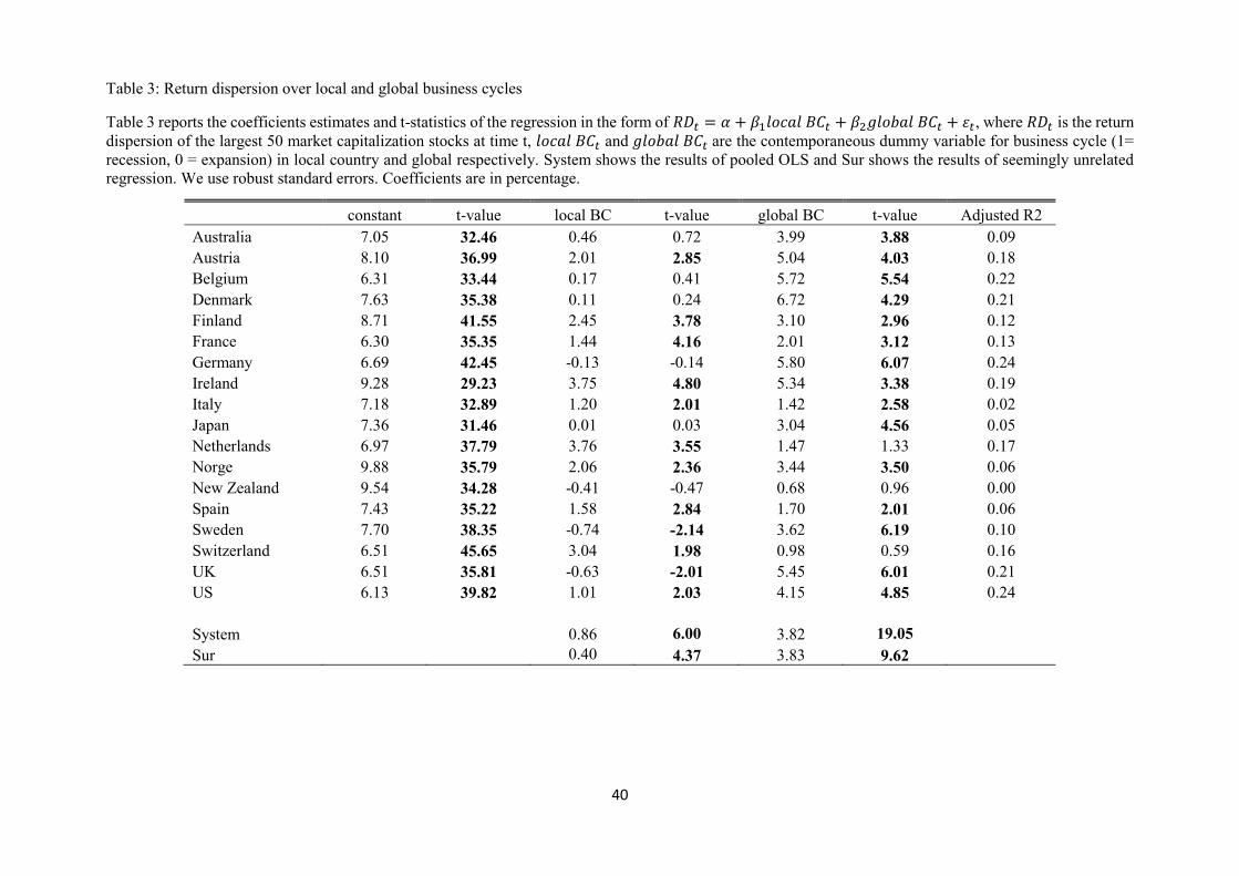
40
Table 3: Return dispersion over local and global business cycles
Table 3 reports the coefficients estimates and t-statistics of the regression in the form of 𝑅𝐷𝑡 = 𝛼 + 𝛽1𝑙𝑜𝑐𝑎𝑙 𝐵𝐶𝑡 + 𝛽2𝑔𝑙𝑜𝑏𝑎𝑙 𝐵𝐶𝑡 + 𝜀𝑡, where 𝑅𝐷𝑡 is the return
dispersion of the largest 50 market capitalization stocks at time t, 𝑙𝑜𝑐𝑎𝑙 𝐵𝐶𝑡 and 𝑔𝑙𝑜𝑏𝑎𝑙 𝐵𝐶𝑡 are the contemporaneous dummy variable for business cycle (1=
recession, 0 = expansion) in local country and global respectively. System shows the results of pooled OLS and Sur shows the results of seemingly unrelated
regression. We use robust standard errors. Coefficients are in percentage.
constant t-value local BC t-value global BC t-value Adjusted R2
Australia 7.05 32.46 0.46 0.72 3.99 3.88 0.09
Austria 8.10 36.99 2.01 2.85 5.04 4.03 0.18
Belgium 6.31 33.44 0.17 0.41 5.72 5.54 0.22
Denmark 7.63 35.38 0.11 0.24 6.72 4.29 0.21
Finland 8.71 41.55 2.45 3.78 3.10 2.96 0.12
France 6.30 35.35 1.44 4.16 2.01 3.12 0.13
Germany 6.69 42.45 -0.13 -0.14 5.80 6.07 0.24
Ireland 9.28 29.23 3.75 4.80 5.34 3.38 0.19
Italy 7.18 32.89 1.20 2.01 1.42 2.58 0.02
Japan 7.36 31.46 0.01 0.03 3.04 4.56 0.05
Netherlands 6.97 37.79 3.76 3.55 1.47 1.33 0.17
Norge 9.88 35.79 2.06 2.36 3.44 3.50 0.06
New Zealand 9.54 34.28 -0.41 -0.47 0.68 0.96 0.00
Spain 7.43 35.22 1.58 2.84 1.70 2.01 0.06
Sweden 7.70 38.35 -0.74 -2.14 3.62 6.19 0.10
Switzerland 6.51 45.65 3.04 1.98 0.98 0.59 0.16
UK 6.51 35.81 -0.63 -2.01 5.45 6.01 0.21
US 6.13 39.82 1.01 2.03 4.15 4.85 0.24
System 0.86 6.00 3.82 19.05 Sur 0.40 4.37 3.83 9.62
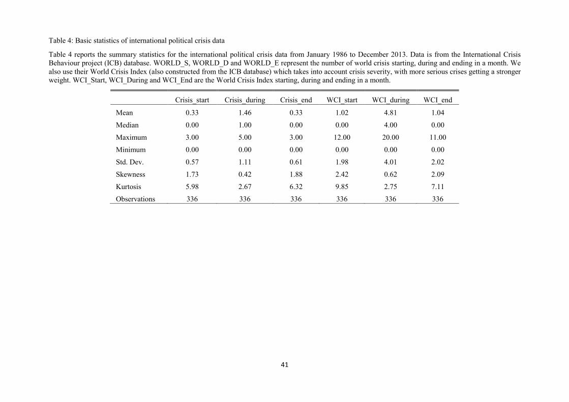
41
Table 4: Basic statistics of international political crisis data
Table 4 reports the summary statistics for the international political crisis data from January 1986 to December 2013. Data is from the International Crisis
Behaviour project (ICB) database. WORLD_S, WORLD_D and WORLD_E represent the number of world crisis starting, during and ending in a month. We
also use their World Crisis Index (also constructed from the ICB database) which takes into account crisis severity, with more serious crises getting a stronger
weight. WCI_Start, WCI_During and WCI_End are the World Crisis Index starting, during and ending in a month.
Crisis_start Crisis_during Crisis_end WCI_start WCI_during WCI_end
Mean 0.33 1.46 0.33 1.02 4.81 1.04
Median 0.00 1.00 0.00 0.00 4.00 0.00
Maximum 3.00 5.00 3.00 12.00 20.00 11.00
Minimum 0.00 0.00 0.00 0.00 0.00 0.00
Std. Dev. 0.57 1.11 0.61 1.98 4.01 2.02
Skewness 1.73 0.42 1.88 2.42 0.62 2.09
Kurtosis 5.98 2.67 6.32 9.85 2.75 7.11
Observations 336 336 336 336 336 336

42
Table 5: Return dispersion and international political crises
Table 5 provides the results of return dispersion regress on world crisis index with the control of business cycle in each country (𝑅𝐷𝑡 = 𝛼 + 𝛽1𝐵𝐶_𝑙𝑜𝑐𝑎𝑙𝑡 +𝛽2𝐵𝐶_𝑔𝑙𝑜𝑏𝑎𝑙𝑡 + 𝛽3𝑆𝑡𝑎𝑟𝑡_𝑊𝐶𝐼𝑡 + 𝛽4𝐷𝑢𝑟𝑖𝑛𝑔_𝑊𝐶𝐼𝑡 + 𝛽5𝐸𝑛𝑑_𝑊𝐶𝐼𝑡 + 𝜀𝑡). 𝑅𝐷𝑡 is the return dispersion of the largest 50 market capitalization stocks in each
country at time t. 𝐵𝐶_𝑙𝑜𝑐𝑎𝑙𝑡 and 𝐵𝐶_𝑔𝑙𝑜𝑏𝑎𝑙𝑡 are the dummy variables for business cycle (1= recession, 0 = expansion) in local country and global respectively.
𝑆𝑡𝑎𝑟𝑡_𝑊𝐶𝐼𝑡, 𝐷𝑢𝑟𝑖𝑛𝑔_𝑊𝐶𝐼𝑡 and 𝐸𝑛𝑑_𝑊𝐶𝐼𝑡 are ongoing crisis starting at month t, during month t and ending at month t. System shows the results of pooled
OLS and Sur shows the results of seemingly unrelated regression. We use robust standard errors. Coefficients are in percentage.
Constant t-value
Local
BC t-value
Global
BC t-value
Start
WCI t-value
During
WCI t-value
End
WCI t-value
Adjusted
R2
Australia 6.49 21.71 0.46 0.69 4.23 4.15 0.18 1.65 0.06 1.03 0.07 0.87 0.10
Austria 8.10 22.54 2.00 2.74 5.05 4.06 -0.05 -0.54 -0.02 -0.38 0.13 0.84 0.18
Belgium 5.93 17.68 0.21 0.50 5.85 5.64 0.07 0.81 0.04 1.10 0.06 0.71 0.22
Denmark 6.99 28.67 0.16 0.36 6.86 4.40 0.06 0.70 0.14 3.63 -0.16 -2.41 0.24
Finland 7.08 22.15 2.24 3.47 3.66 3.45 0.14 1.74 0.29 6.29 -0.01 -0.12 0.22
France 5.57 28.38 1.19 3.31 2.40 3.59 0.10 1.13 0.13 3.57 0.02 0.18 0.16
Germany 6.33 28.01 -0.19 -0.19 5.94 6.20 0.10 1.16 0.05 1.67 -0.03 -0.29 0.24
Ireland 7.95 17.32 3.91 4.96 5.66 3.50 0.25 1.38 0.22 3.17 -0.11 -0.90 0.22
Italy 6.79 16.47 1.01 1.69 1.59 2.69 -0.04 -0.44 0.08 1.35 0.05 0.52 0.02
Japan 6.35 20.43 -0.04 -0.08 3.39 5.15 0.15 1.44 0.16 3.22 0.00 -0.02 0.08
Netherlands 6.34 19.27 3.58 3.33 1.78 1.58 0.15 1.23 0.12 2.50 -0.12 -1.08 0.18
Norge 9.03 17.52 1.99 2.20 3.69 3.65 0.10 0.77 0.16 2.49 -0.09 -0.87 0.08
New Zealand 8.00 16.11 -0.26 -0.30 1.18 1.65 0.29 1.70 0.23 4.00 -0.01 -0.13 0.05
Spain 5.89 22.98 1.13 2.08 2.61 2.97 0.39 3.47 0.17 3.90 0.23 1.97 0.16
Sweden 6.02 24.49 -0.52 -1.62 4.08 6.79 0.22 1.95 0.24 6.42 0.11 1.18 0.23
Switzerland 5.91 24.29 3.08 2.02 1.13 0.69 0.02 0.23 0.09 2.26 0.09 0.97 0.17
UK 5.87 24.66 -0.48 -1.57 5.56 6.21 0.20 2.48 0.12 3.70 -0.19 -2.87 0.26
US 5.33 31.70 0.89 1.79 4.47 5.24 0.00 -0.05 0.15 4.47 0.01 0.15 0.28
System
0.83 5.85 4.11 20.59 0.13 5.15 0.14 11.14 0.00 0.12
Sur
0.40 4.36 4.06 10.69 0.10 2.01 0.16 6.34 0.06 1.23

43
Table 6: Return dispersion and word count uncertainty
Table 6 reports the regression of return dispersion on word count uncertainty around the world. We count the number of Bloomberg reports in every month that
contains the word “uncertainty” and take a log of it. We consider these word counts as proxy for uncertainty. We run the regression in the form of 𝑅𝐷𝑡 = 𝛼 +𝛽1𝑙𝑜𝑐𝑎𝑙_𝐵𝐶𝑡 + 𝛽2𝑔𝑙𝑜𝑏𝑎𝑙_𝐵𝐶𝑡 + 𝛽3𝑆𝑡𝑎𝑟𝑡𝑡 + 𝛽4𝐷𝑢𝑟𝑖𝑛𝑔𝑡 + 𝛽5𝐸𝑛𝑑𝑡 + 𝛽6 𝑙𝑛(𝑤𝑜𝑟𝑑 𝑐𝑜𝑢𝑛𝑡 𝑢𝑛𝑐𝑒𝑟𝑡𝑎𝑖𝑛𝑡𝑦)𝑡 + 𝜀𝑡 where BC is the business cycle dummy, Start is
crisis starting in month t, During is the ongoing crisis in month t and End is the crisis ending in month t. System shows the results of pooled OLS and Sur shows
the results of seemingly unrelated regression. We use robust standard errors. Coefficients are in percentage.
constant t-stat
local
BC t-stat
global
BC t-stat
start
Crisis t-stat
during
Crisis t-stat
end
Crisis t-stat
Word Count
Uncertainty t-stat
Adjust
ed R2
Australia 9.69 7.21 0.08 0.11 5.07 4.83 0.13 1.15 0.04 0.78 0.02 0.22 -0.48 -2.45 0.12
Austria 4.90 4.09 1.95 2.72 4.36 3.46 0.01 0.07 -0.01 -0.11 0.19 1.21 0.49 2.80 0.20
Belgium 1.60 1.22 0.70 1.55 4.73 4.57 0.15 1.78 0.06 1.49 0.14 1.63 0.64 3.91 0.27
Denmark 2.10 2.39 0.61 1.32 5.66 3.69 0.14 1.71 0.17 4.18 -0.07 -1.15 0.72 5.72 0.28
Finland 7.04 5.21 2.24 3.25 3.64 3.23 0.14 1.64 0.29 6.14 -0.01 -0.11 0.01 0.03 0.22
France 3.11 3.56 1.30 3.73 1.78 2.49 0.15 1.57 0.14 3.81 0.06 0.64 0.37 2.91 0.19
Germany 1.35 1.65 0.67 0.69 4.51 4.86 0.18 2.16 0.07 2.34 0.05 0.53 0.75 6.09 0.32
Ireland 5.71 3.67 3.73 4.67 5.24 3.10 0.29 1.51 0.23 3.27 -0.07 -0.59 0.35 1.48 0.22
Italy 4.29 5.26 1.30 2.24 0.91 1.31 0.00 0.04 0.08 1.52 0.09 0.92 0.38 2.60 0.04
Japan 3.04 2.72 0.06 0.12 2.58 3.69 0.20 1.98 0.18 3.35 0.06 0.62 0.50 3.20 0.11
Netherlands 0.86 0.71 3.47 3.49 0.62 0.52 0.24 2.08 0.14 3.20 -0.03 -0.25 0.83 4.41 0.24
Norge 7.12 4.33 1.94 2.18 3.27 3.15 0.14 0.96 0.17 2.54 -0.06 -0.53 0.29 1.33 0.08
New
Zealand 16.65 10.35 0.07 0.09 3.14 4.17 0.15 0.87 0.20 3.76 -0.16 -1.55 -1.32 -5.78 0.19
Spain 9.51 9.42 1.23 2.14 3.36 3.74 0.32 3.08 0.16 3.62 0.16 1.41 -0.55 -3.82 0.20
Sweden 5.40 6.37 -0.56 -1.71 3.95 6.21 0.24 2.03 0.25 6.46 0.13 1.23 0.09 0.75 0.23
Switzerland 1.71 1.58 2.65 1.90 0.56 0.35 0.09 1.31 0.11 2.56 0.16 1.87 0.64 4.36 0.23
UK 1.46 1.74 0.04 0.14 4.30 4.70 0.27 3.56 0.14 4.56 -0.12 -1.81 0.65 5.25 0.33
US 0.05 0.07 1.12 3.29 3.06 3.87 0.09 1.76 0.17 5.59 0.10 1.39 0.80 7.33 0.40
System 0.89 6.30 3.64 17.43 0.16 6.41 0.15 11.75 0.04 1.50 0.30 7.37 0.89
Sur 0.41 4.51 3.91 9.85 0.11 2.18 0.16 6.41 0.07 1.48 0.23 2.84

44
Table 7: Return dispersion and international country risk
Table 7 presents the relation between return dispersion and international country risk. We take the International Country Risk Guide (ICRG) composite index
as another measure of country-level uncertainty. We run the regression in the form of 𝑅𝐷𝑡 = 𝛼 + 𝛽1𝐵𝐶_𝑙𝑜𝑐𝑎𝑙𝑡 + 𝛽2𝐵𝐶_𝑔𝑙𝑜𝑏𝑎𝑙𝑡 + 𝛽3𝑆𝑡𝑎𝑟𝑡_𝑊𝐶𝐼𝑡 +𝛽4𝐷𝑢𝑟𝑖𝑛𝑔_𝑊𝐶𝐼𝑡 + 𝛽5𝐸𝑛𝑑_𝑊𝐶𝐼𝑡 + 𝛽6𝑊𝑜𝑟𝑑𝐶𝑜𝑢𝑛𝑡𝑡 + 𝛽7𝐶𝑜𝑢𝑛𝑡𝑟𝑦_𝑅𝑖𝑠𝑘𝑡 + 𝜀𝑡. 𝐵𝐶_𝑙𝑜𝑐𝑎𝑙𝑡 and 𝐵𝐶_𝑔𝑙𝑜𝑏𝑎𝑙𝑡 are the dummy variables for business cycle (1=
recession, 0 = expansion) in local country and global respectively. 𝑆𝑡𝑎𝑟𝑡_𝑊𝐶𝐼𝑡, 𝐷𝑢𝑟𝑖𝑛𝑔_𝑊𝐶𝐼𝑡 and 𝐸𝑛𝑑_𝑊𝐶𝐼𝑡 are ongoing crisis starting at month t, during
month t and ending at month t. 𝑊𝑜𝑟𝑑𝐶𝑜𝑢𝑛𝑡𝑡 is the log number of the counts of Bloomberg reports in every month that contains the word “uncertainty”. System
shows the results of pooled OLS and Sur shows the results of seemingly unrelated regression. We use robust standard errors. Coefficients are in percentage.
constant t-stat
local
BC t-stat
global
BC t-stat
start
Crisis t-stat
during
Crisis t-stat
end
Crisis t-stat
word
count
uncertainty t-stat
Country
Risk t-stat
Adjusted
R2
Australia 48.24 5.61 0.45 0.69 3.68 3.77 0.04 0.43 0.00 0.05 0.00 -0.04 -0.10 -0.56 -0.50 -4.81 0.17
Austria 0.06 0.01 1.98 2.77 4.40 3.49 0.01 0.10 -0.01 -0.14 0.19 1.22 0.51 2.85 0.05 0.52 0.20
Belgium 38.08 4.16 0.21 0.47 3.92 4.39 0.11 1.31 -0.02 -0.44 0.11 1.25 0.80 5.32 -0.45 -4.30 0.32
Denmark 15.21 2.33 0.64 1.39 5.46 3.62 0.14 1.77 0.16 4.08 -0.07 -1.12 0.92 5.39 -0.17 -2.00 0.29
Finland 8.63 1.13 2.25 3.24 3.63 3.19 0.15 1.65 0.29 6.04 -0.01 -0.08 0.04 0.17 -0.02 -0.21 0.22
France -15.56 -2.16 1.15 3.18 2.04 2.75 0.17 1.83 0.12 3.41 0.07 0.81 0.49 3.34 0.23 2.75 0.21
Germany -10.32 -1.24 2.32 2.07 3.26 3.68 0.08 0.69 0.18 4.54 0.02 0.14 1.63 7.53 0.06 0.62 0.39
Ireland 32.52 4.34 3.39 4.44 4.29 2.73 0.30 1.55 0.18 2.52 -0.05 -0.45 1.10 4.25 -0.38 -3.93 0.26
Italy 3.03 0.59 1.34 2.16 0.90 1.30 0.00 0.02 0.08 1.50 0.09 0.91 0.38 2.59 0.02 0.25 0.03
Japan -3.68 -0.57 0.11 0.25 2.64 3.74 0.21 2.02 0.19 3.54 0.06 0.66 0.60 3.46 0.07 1.04 0.11
Netherlands -30.10 -2.78 2.75 3.08 0.67 0.56 0.21 1.89 0.14 3.33 -0.04 -0.41 1.09 4.78 0.34 2.97 0.26
Norge 4.22 0.39 1.93 2.16 3.31 3.20 0.14 0.94 0.18 2.58 -0.06 -0.53 0.24 0.88 0.04 0.27 0.08
New
Zealand 50.14 4.33 0.43 0.54 2.19 2.87 0.09 0.51 0.16 3.08 -0.17 -1.65 -1.69 -6.30 -0.38 -2.98 0.22
Spain 21.98 3.68 1.06 1.87 3.02 3.73 0.32 2.99 0.15 3.42 0.16 1.38 -0.36 -2.23 -0.18 -2.17 0.21
Sweden 19.87 3.72 -0.64 -1.90 3.96 6.51 0.24 2.05 0.21 5.54 0.12 1.21 0.17 1.30 -0.17 -2.76 0.24
Switzerland -43.27 -3.27 2.26 1.89 1.07 0.74 0.06 1.02 0.14 2.99 0.13 1.81 1.10 4.64 0.47 3.57 0.29
UK -9.94 -1.92 -0.08 -0.25 4.62 4.78 0.28 3.68 0.14 4.75 -0.12 -1.88 0.69 5.51 0.14 2.27 0.34
US -20.66 -5.57 1.33 4.65 2.64 3.36 0.08 1.68 0.13 4.41 0.10 1.34 1.25 9.13 0.22 5.85 0.44
System 0.88 6.23 3.70 17.59 0.16 6.29 0.15 11.93 0.04 1.51 0.29 7.03 0.05 3.84 Sur 0.41 4.35 3.88 9.81 0.11 2.46 0.15 6.36 0.06 1.22 0.27 3.67 0.05 5.51

45
Table 8: Return dispersion and economic policy uncertainty
Table 8 presents the characteristics of economic policy uncertainty. We show the results for the regression: 𝑅𝐷𝑡 = 𝛼 + 𝛽1𝐵𝐶_𝑙𝑜𝑐𝑎𝑙𝑡 + 𝛽2𝐵𝐶_𝑔𝑙𝑜𝑏𝑎𝑙𝑡 +𝛽3𝑆𝑡𝑎𝑟𝑡_𝑊𝐶𝐼𝑡 + 𝛽4𝐷𝑢𝑟𝑖𝑛𝑔_𝑊𝐶𝐼𝑡 + 𝛽5𝐸𝑛𝑑_𝑊𝐶𝐼𝑡 + 𝛽6𝑊𝑜𝑟𝑑𝐶𝑜𝑢𝑛𝑡𝑡 + 𝛽7𝐶𝑜𝑢𝑛𝑡𝑟𝑦_𝑅𝑖𝑠𝑘𝑡 + 𝛽8ln (𝐸𝑃𝑈_𝑙𝑜𝑐𝑎𝑙)𝑡 +𝛽9ln (𝐸𝑃𝑈_𝑔𝑙𝑜𝑏𝑎𝑙)𝑡 + 𝜀𝑡 𝑅𝐷𝑡 is the
return dispersion of the largest 50 market capitalization stocks in each country at time t. 𝐵𝐶_𝑙𝑜𝑐𝑎𝑙𝑡 and 𝐵𝐶_𝑔𝑙𝑜𝑏𝑎𝑙𝑡 are the dummy variables for business cycle
(1= recession, 0 = expansion) in local country and global respectively. 𝑆𝑡𝑎𝑟𝑡_𝑊𝐶𝐼𝑡, 𝐷𝑢𝑟𝑖𝑛𝑔_𝑊𝐶𝐼𝑡 and 𝐸𝑛𝑑_𝑊𝐶𝐼𝑡 are ongoing crisis starting at month t, during
month t and ending at month t. 𝑊𝑜𝑟𝑑𝐶𝑜𝑢𝑛𝑡𝑡 is the log number of the counts of Bloomberg reports in every month that contains the word “uncertainty”.
𝐶𝑜𝑢𝑛𝑡𝑟𝑦_𝑅𝑖𝑠𝑘𝑡 represents the ICRG composite risk index for each country. We include two economic policy index, one is the country specific index
(𝐸𝑃𝑈_𝑙𝑜𝑐𝑎𝑙) and the other is the global index (𝐸𝑃𝑈_𝑔𝑙𝑜𝑏𝑎𝑙). System shows the results of pooled OLS and Sur shows the results of seemingly unrelated
regression. We use robust standard errors. Coefficients are in percentage.
Country Coefficient Constant
Local
BC
Global
BC
Start
WCI
during
WCI
end
WCI
Word Count
Uncertainty
Country
Risk
ln(Local
EPU)
ln(Global
EPU) N
Adjusted
R2
Australia Coeff. (%) 7.19 2.29 2.14 0.09 -0.09 0.22 0.34 -0.09 3.60 -2.48 144 0.35
t-Stat 0.53 1.10 2.26 0.61 -1.03 1.30 0.62 -0.58 4.06 -1.80 France Coeff. (%) -28.61 0.49 1.12 0.06 0.29 -0.02 -0.19 0.19 -0.41 5.09 156 0.43
t-Stat -2.03 0.55 1.45 0.38 3.59 -0.12 -0.36 1.36 -0.83 4.72 Germany Coeff. (%) -9.71 2.22 2.46 -0.07 0.24 0.01 -0.04 -0.11 0.59 5.21 156 0.46
t-Stat -0.77 1.11 2.60 -0.51 3.96 0.06 -0.09 -0.81 0.85 4.73 Ireland Coeff. (%) -8.05 2.63 3.33 0.40 0.09 -0.01 1.02 -0.19 1.76 4.16 156 0.29
t-Stat -0.48 2.84 2.33 0.97 0.76 -0.03 1.29 -1.38 1.57 2.13 Italy Coeff. (%) -2.24 1.22 0.96 -0.06 0.15 0.05 -0.82 -0.05 2.16 2.13 156 0.07
t-Stat -0.21 1.34 1.60 -0.47 1.37 0.20 -1.75 -0.45 2.70 1.98 Japan Coeff. (%) -17.71 0.23 2.23 0.08 0.41 -0.09 0.71 0.16 2.49 -1.36 156 0.18
t-Stat -1.51 0.34 2.65 0.51 4.39 -0.67 1.04 1.61 2.51 -0.89 Netherland Coeff. (%) 10.51 3.29 0.93 -0.07 0.02 -0.26 -1.71 -0.15 -0.74 5.71 82 0.53
t-Stat 0.71 1.86 0.97 -0.44 0.16 -1.92 -2.22 -0.96 -0.81 3.62 Spain Coeff. (%) 14.50 1.19 1.56 0.18 0.22 0.22 -1.24 -0.23 -0.85 4.92 108 0.41
t-Stat 1.06 1.60 1.51 0.86 2.35 1.04 -1.43 -1.76 -1.33 3.53 Sweden Coeff. (%) 13.45 -0.51 2.70 0.08 0.18 0.15 1.24 -0.34 1.29 1.64 156 0.39
t-Stat 1.22 -1.16 4.55 0.55 3.17 0.78 2.03 -2.95 0.99 1.53 UK Coeff. (%) -16.71 -0.11 2.88 0.17 0.22 -0.25 0.21 -0.02 -2.36 7.66 156 0.48
t-Stat -2.06 -0.23 3.37 1.31 4.28 -2.18 0.46 -0.33 -3.17 6.40 US Coeff. (%) -39.18 1.22 1.65 0.01 0.25 0.11 0.58 0.31 3.74 -0.02 156 0.49
t-Stat -6.40 2.74 2.32 0.07 3.88 0.68 1.42 6.25 2.27 -0.01 System Coeff. (%) 1.23 2.35 0.07 0.24 0.03 0.06 0.13 0.64 3.21
t-Stat 4.87 7.90 1.17 9.57 0.49 0.28 5.69 2.60 7.74 Sur Coeff. (%) 0.53 2.70 0.03 0.21 0.09 -0.05 0.11 0.49 3.21 t-Stat 3.15 6.91 0.31 6.11 1.24 -0.19 7.13 2.87 6.31
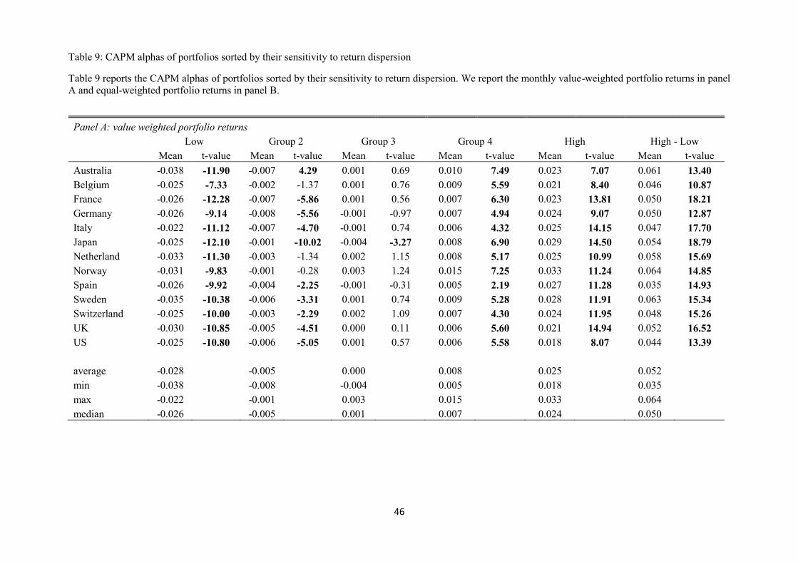
46
Table 9: CAPM alphas of portfolios sorted by their sensitivity to return dispersion
Table 9 reports the CAPM alphas of portfolios sorted by their sensitivity to return dispersion. We report the monthly value-weighted portfolio returns in panel
A and equal-weighted portfolio returns in panel B.
Panel A: value weighted portfolio returns
Low Group 2 Group 3 Group 4 High High - Low
Mean t-value Mean t-value Mean t-value Mean t-value Mean t-value Mean t-value
Australia -0.038 -11.90 -0.007 4.29 0.001 0.69 0.010 7.49 0.023 7.07 0.061 13.40
Belgium -0.025 -7.33 -0.002 -1.37 0.001 0.76 0.009 5.59 0.021 8.40 0.046 10.87
France -0.026 -12.28 -0.007 -5.86 0.001 0.56 0.007 6.30 0.023 13.81 0.050 18.21
Germany -0.026 -9.14 -0.008 -5.56 -0.001 -0.97 0.007 4.94 0.024 9.07 0.050 12.87
Italy -0.022 -11.12 -0.007 -4.70 -0.001 0.74 0.006 4.32 0.025 14.15 0.047 17.70
Japan -0.025 -12.10 -0.001 -10.02 -0.004 -3.27 0.008 6.90 0.029 14.50 0.054 18.79
Netherland -0.033 -11.30 -0.003 -1.34 0.002 1.15 0.008 5.17 0.025 10.99 0.058 15.69
Norway -0.031 -9.83 -0.001 -0.28 0.003 1.24 0.015 7.25 0.033 11.24 0.064 14.85
Spain -0.026 -9.92 -0.004 -2.25 -0.001 -0.31 0.005 2.19 0.027 11.28 0.035 14.93
Sweden -0.035 -10.38 -0.006 -3.31 0.001 0.74 0.009 5.28 0.028 11.91 0.063 15.34
Switzerland -0.025 -10.00 -0.003 -2.29 0.002 1.09 0.007 4.30 0.024 11.95 0.048 15.26
UK -0.030 -10.85 -0.005 -4.51 0.000 0.11 0.006 5.60 0.021 14.94 0.052 16.52
US -0.025 -10.80 -0.006 -5.05 0.001 0.57 0.006 5.58 0.018 8.07 0.044 13.39
average -0.028 -0.005 0.000 0.008 0.025 0.052 min -0.038 -0.008 -0.004 0.005 0.018 0.035 max -0.022 -0.001 0.003 0.015 0.033 0.064 median -0.026 -0.005 0.001 0.007 0.024 0.050
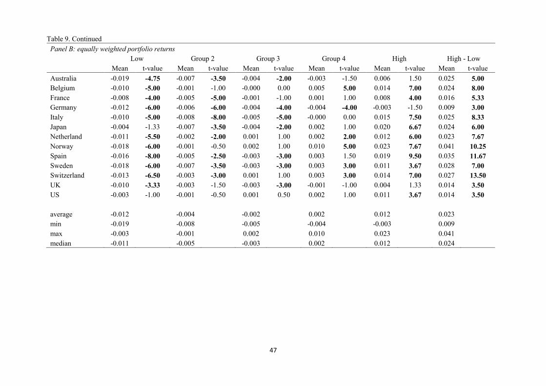
47
Table 9. Continued
Panel B: equally weighted portfolio returns
Low Group 2 Group 3 Group 4 High High - Low
Mean t-value Mean t-value Mean t-value Mean t-value Mean t-value Mean t-value
Australia -0.019 -4.75 -0.007 -3.50 -0.004 -2.00 -0.003 -1.50 0.006 1.50 0.025 5.00
Belgium -0.010 -5.00 -0.001 -1.00 -0.000 0.00 0.005 5.00 0.014 7.00 0.024 8.00
France -0.008 -4.00 -0.005 -5.00 -0.001 -1.00 0.001 1.00 0.008 4.00 0.016 5.33
Germany -0.012 -6.00 -0.006 -6.00 -0.004 -4.00 -0.004 -4.00 -0.003 -1.50 0.009 3.00
Italy -0.010 -5.00 -0.008 -8.00 -0.005 -5.00 -0.000 0.00 0.015 7.50 0.025 8.33
Japan -0.004 -1.33 -0.007 -3.50 -0.004 -2.00 0.002 1.00 0.020 6.67 0.024 6.00
Netherland -0.011 -5.50 -0.002 -2.00 0.001 1.00 0.002 2.00 0.012 6.00 0.023 7.67
Norway -0.018 -6.00 -0.001 -0.50 0.002 1.00 0.010 5.00 0.023 7.67 0.041 10.25
Spain -0.016 -8.00 -0.005 -2.50 -0.003 -3.00 0.003 1.50 0.019 9.50 0.035 11.67
Sweden -0.018 -6.00 -0.007 -3.50 -0.003 -3.00 0.003 3.00 0.011 3.67 0.028 7.00
Switzerland -0.013 -6.50 -0.003 -3.00 0.001 1.00 0.003 3.00 0.014 7.00 0.027 13.50
UK -0.010 -3.33 -0.003 -1.50 -0.003 -3.00 -0.001 -1.00 0.004 1.33 0.014 3.50
US -0.003 -1.00 -0.001 -0.50 0.001 0.50 0.002 1.00 0.011 3.67 0.014 3.50
average -0.012 -0.004 -0.002 0.002 0.012 0.023 min -0.019 -0.008 -0.005 -0.004 -0.003 0.009 max -0.003 -0.001 0.002 0.010 0.023 0.041 median -0.011 -0.005 -0.003 0.002 0.012 0.024
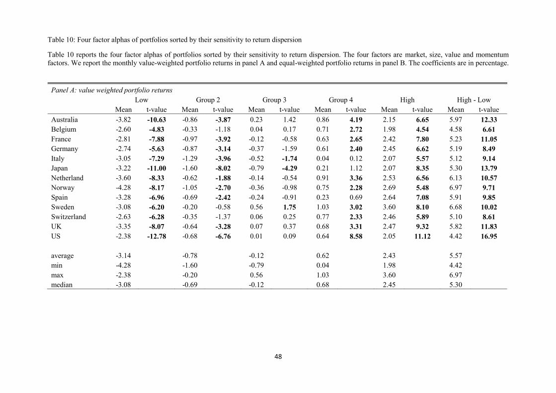
48
Table 10: Four factor alphas of portfolios sorted by their sensitivity to return dispersion
Table 10 reports the four factor alphas of portfolios sorted by their sensitivity to return dispersion. The four factors are market, size, value and momentum
factors. We report the monthly value-weighted portfolio returns in panel A and equal-weighted portfolio returns in panel B. The coefficients are in percentage.
Panel A: value weighted portfolio returns
Low Group 2 Group 3 Group 4 High High - Low
Mean t-value Mean t-value Mean t-value Mean t-value Mean t-value Mean t-value
Australia -3.82 -10.63 -0.86 -3.87 0.23 1.42 0.86 4.19 2.15 6.65 5.97 12.33
Belgium -2.60 -4.83 -0.33 -1.18 0.04 0.17 0.71 2.72 1.98 4.54 4.58 6.61
France -2.81 -7.88 -0.97 -3.92 -0.12 -0.58 0.63 2.65 2.42 7.80 5.23 11.05
Germany -2.74 -5.63 -0.87 -3.14 -0.37 -1.59 0.61 2.40 2.45 6.62 5.19 8.49
Italy -3.05 -7.29 -1.29 -3.96 -0.52 -1.74 0.04 0.12 2.07 5.57 5.12 9.14
Japan -3.22 -11.00 -1.60 -8.02 -0.79 -4.29 0.21 1.12 2.07 8.35 5.30 13.79
Netherland -3.60 -8.33 -0.62 -1.88 -0.14 -0.54 0.91 3.36 2.53 6.56 6.13 10.57
Norway -4.28 -8.17 -1.05 -2.70 -0.36 -0.98 0.75 2.28 2.69 5.48 6.97 9.71
Spain -3.28 -6.96 -0.69 -2.42 -0.24 -0.91 0.23 0.69 2.64 7.08 5.91 9.85
Sweden -3.08 -6.20 -0.20 -0.58 0.56 1.75 1.03 3.02 3.60 8.10 6.68 10.02
Switzerland -2.63 -6.28 -0.35 -1.37 0.06 0.25 0.77 2.33 2.46 5.89 5.10 8.61
UK -3.35 -8.07 -0.64 -3.28 0.07 0.37 0.68 3.31 2.47 9.32 5.82 11.83
US -2.38 -12.78 -0.68 -6.76 0.01 0.09 0.64 8.58 2.05 11.12 4.42 16.95
average -3.14 -0.78 -0.12 0.62 2.43 5.57 min -4.28 -1.60 -0.79 0.04 1.98 4.42 max -2.38 -0.20 0.56 1.03 3.60 6.97 median -3.08 -0.69 -0.12 0.68 2.45 5.30
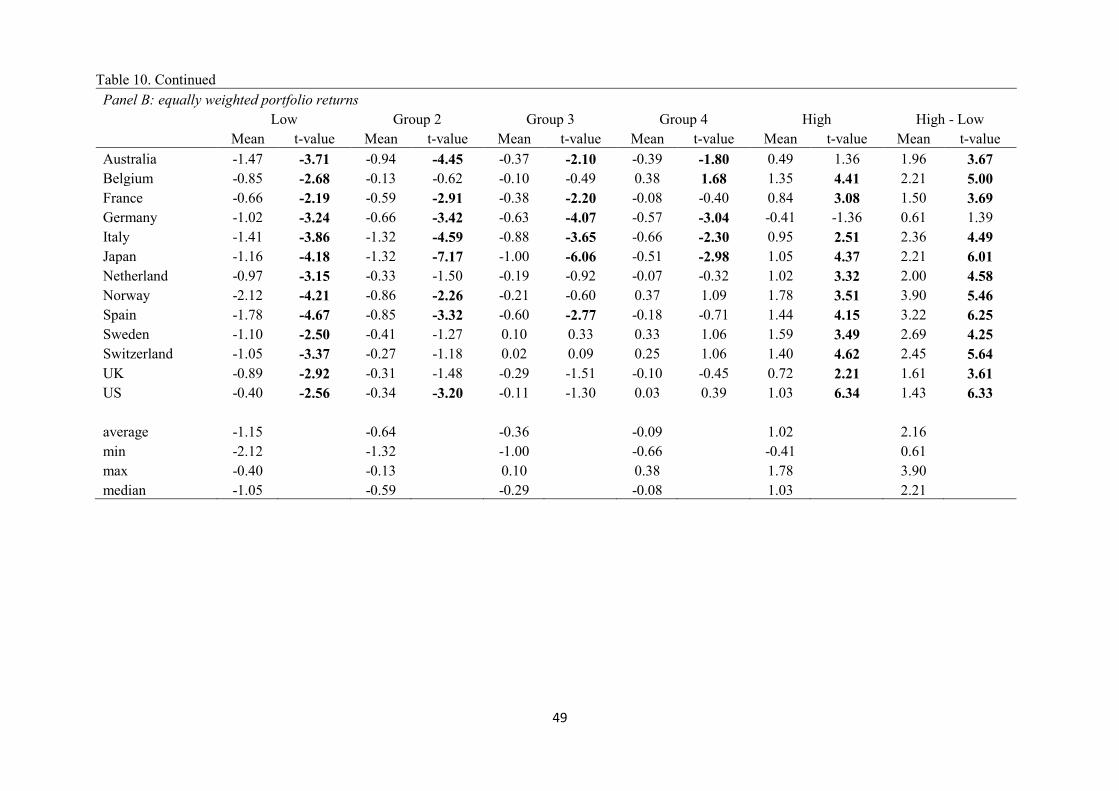
49
Table 10. Continued
Panel B: equally weighted portfolio returns
Low Group 2 Group 3 Group 4 High High - Low
Mean t-value Mean t-value Mean t-value Mean t-value Mean t-value Mean t-value
Australia -1.47 -3.71 -0.94 -4.45 -0.37 -2.10 -0.39 -1.80 0.49 1.36 1.96 3.67
Belgium -0.85 -2.68 -0.13 -0.62 -0.10 -0.49 0.38 1.68 1.35 4.41 2.21 5.00
France -0.66 -2.19 -0.59 -2.91 -0.38 -2.20 -0.08 -0.40 0.84 3.08 1.50 3.69
Germany -1.02 -3.24 -0.66 -3.42 -0.63 -4.07 -0.57 -3.04 -0.41 -1.36 0.61 1.39
Italy -1.41 -3.86 -1.32 -4.59 -0.88 -3.65 -0.66 -2.30 0.95 2.51 2.36 4.49
Japan -1.16 -4.18 -1.32 -7.17 -1.00 -6.06 -0.51 -2.98 1.05 4.37 2.21 6.01
Netherland -0.97 -3.15 -0.33 -1.50 -0.19 -0.92 -0.07 -0.32 1.02 3.32 2.00 4.58
Norway -2.12 -4.21 -0.86 -2.26 -0.21 -0.60 0.37 1.09 1.78 3.51 3.90 5.46
Spain -1.78 -4.67 -0.85 -3.32 -0.60 -2.77 -0.18 -0.71 1.44 4.15 3.22 6.25
Sweden -1.10 -2.50 -0.41 -1.27 0.10 0.33 0.33 1.06 1.59 3.49 2.69 4.25
Switzerland -1.05 -3.37 -0.27 -1.18 0.02 0.09 0.25 1.06 1.40 4.62 2.45 5.64
UK -0.89 -2.92 -0.31 -1.48 -0.29 -1.51 -0.10 -0.45 0.72 2.21 1.61 3.61
US -0.40 -2.56 -0.34 -3.20 -0.11 -1.30 0.03 0.39 1.03 6.34 1.43 6.33
average -1.15 -0.64 -0.36 -0.09 1.02 2.16 min -2.12 -1.32 -1.00 -0.66 -0.41 0.61 max -0.40 -0.13 0.10 0.38 1.78 3.90 median -1.05 -0.59 -0.29 -0.08 1.03 2.21
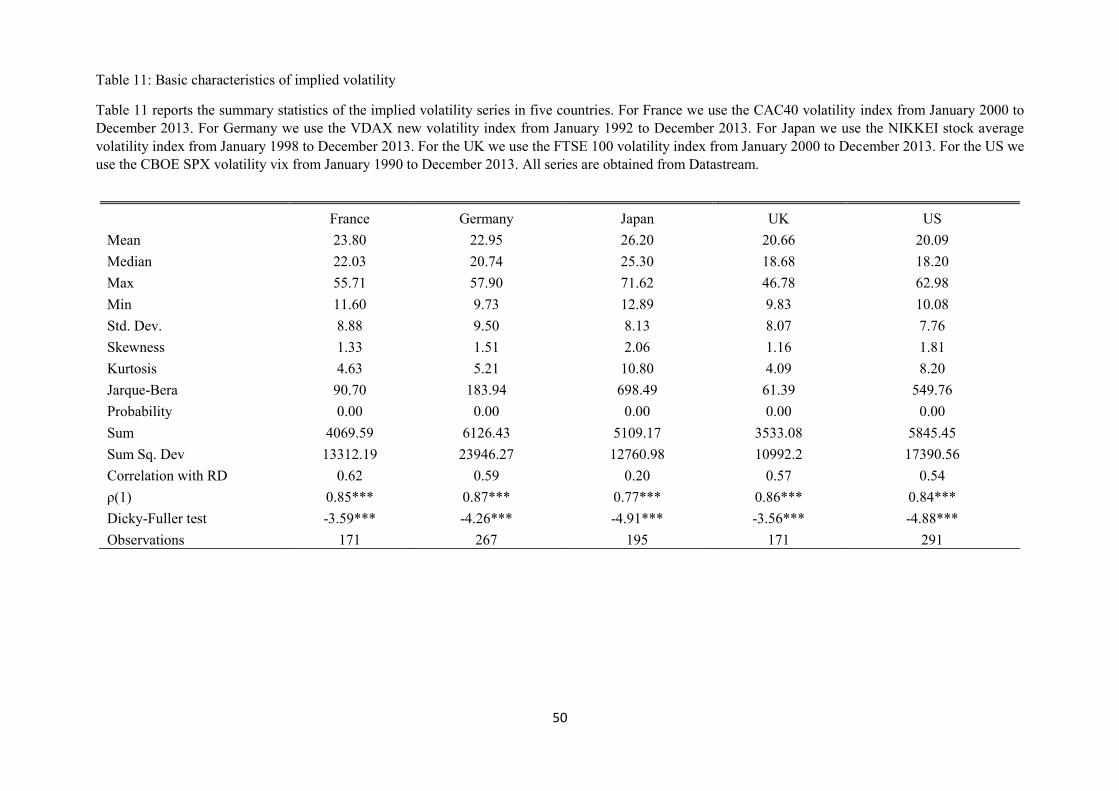
50
Table 11: Basic characteristics of implied volatility
Table 11 reports the summary statistics of the implied volatility series in five countries. For France we use the CAC40 volatility index from January 2000 to
December 2013. For Germany we use the VDAX new volatility index from January 1992 to December 2013. For Japan we use the NIKKEI stock average
volatility index from January 1998 to December 2013. For the UK we use the FTSE 100 volatility index from January 2000 to December 2013. For the US we
use the CBOE SPX volatility vix from January 1990 to December 2013. All series are obtained from Datastream.
France Germany Japan UK US
Mean 23.80 22.95 26.20 20.66 20.09
Median 22.03 20.74 25.30 18.68 18.20
Max 55.71 57.90 71.62 46.78 62.98
Min 11.60 9.73 12.89 9.83 10.08
Std. Dev. 8.88 9.50 8.13 8.07 7.76
Skewness 1.33 1.51 2.06 1.16 1.81
Kurtosis 4.63 5.21 10.80 4.09 8.20
Jarque-Bera 90.70 183.94 698.49 61.39 549.76
Probability 0.00 0.00 0.00 0.00 0.00
Sum 4069.59 6126.43 5109.17 3533.08 5845.45
Sum Sq. Dev 13312.19 23946.27 12760.98 10992.2 17390.56
Correlation with RD 0.62 0.59 0.20 0.57 0.54
ρ(1) 0.85*** 0.87*** 0.77*** 0.86*** 0.84***
Dicky-Fuller test -3.59*** -4.26*** -4.91*** -3.56*** -4.88***
Observations 171 267 195 171 291
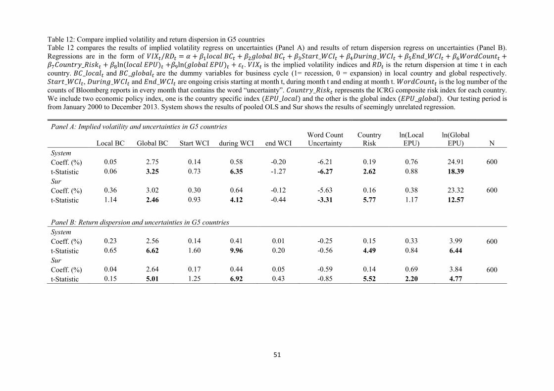
51
Table 12: Compare implied volatility and return dispersion in G5 countries
Table 12 compares the results of implied volatility regress on uncertainties (Panel A) and results of return dispersion regress on uncertainties (Panel B).
Regressions are in the form of 𝑉𝐼𝑋𝑡/𝑅𝐷𝑡 = 𝛼 + 𝛽1𝑙𝑜𝑐𝑎𝑙 𝐵𝐶𝑡 + 𝛽2𝑔𝑙𝑜𝑏𝑎𝑙 𝐵𝐶𝑡 + 𝛽3𝑆𝑡𝑎𝑟𝑡_𝑊𝐶𝐼𝑡 + 𝛽4𝐷𝑢𝑟𝑖𝑛𝑔_𝑊𝐶𝐼𝑡 + 𝛽5𝐸𝑛𝑑_𝑊𝐶𝐼𝑡 + 𝛽6𝑊𝑜𝑟𝑑𝐶𝑜𝑢𝑛𝑡𝑡 +𝛽7𝐶𝑜𝑢𝑛𝑡𝑟𝑦_𝑅𝑖𝑠𝑘𝑡 + 𝛽8ln (𝑙𝑜𝑐𝑎𝑙 𝐸𝑃𝑈)𝑡 +𝛽9ln (𝑔𝑙𝑜𝑏𝑎𝑙 𝐸𝑃𝑈)𝑡 + 𝜀𝑡. 𝑉𝐼𝑋𝑡 is the implied volatility indices and 𝑅𝐷𝑡 is the return dispersion at time t in each
country. 𝐵𝐶_𝑙𝑜𝑐𝑎𝑙𝑡 and 𝐵𝐶_𝑔𝑙𝑜𝑏𝑎𝑙𝑡 are the dummy variables for business cycle (1= recession, 0 = expansion) in local country and global respectively.
𝑆𝑡𝑎𝑟𝑡_𝑊𝐶𝐼𝑡, 𝐷𝑢𝑟𝑖𝑛𝑔_𝑊𝐶𝐼𝑡 and 𝐸𝑛𝑑_𝑊𝐶𝐼𝑡 are ongoing crisis starting at month t, during month t and ending at month t. 𝑊𝑜𝑟𝑑𝐶𝑜𝑢𝑛𝑡𝑡 is the log number of the
counts of Bloomberg reports in every month that contains the word “uncertainty”. 𝐶𝑜𝑢𝑛𝑡𝑟𝑦_𝑅𝑖𝑠𝑘𝑡 represents the ICRG composite risk index for each country.
We include two economic policy index, one is the country specific index (𝐸𝑃𝑈_𝑙𝑜𝑐𝑎𝑙) and the other is the global index (𝐸𝑃𝑈_𝑔𝑙𝑜𝑏𝑎𝑙). Our testing period is
from January 2000 to December 2013. System shows the results of pooled OLS and Sur shows the results of seemingly unrelated regression.
Panel A: Implied volatility and uncertainties in G5 countries
Local BC Global BC Start WCI during WCI end WCI
Word Count
Uncertainty
Country
Risk
ln(Local
EPU)
ln(Global
EPU) N
System Coeff. (%) 0.05 2.75 0.14 0.58 -0.20 -6.21 0.19 0.76 24.91 600
t-Statistic 0.06 3.25 0.73 6.35 -1.27 -6.27 2.62 0.88 18.39 Sur Coeff. (%) 0.36 3.02 0.30 0.64 -0.12 -5.63 0.16 0.38 23.32 600
t-Statistic 1.14 2.46 0.93 4.12 -0.44 -3.31 5.77 1.17 12.57
Panel B: Return dispersion and uncertainties in G5 countries System Coeff. (%) 0.23 2.56 0.14 0.41 0.01 -0.25 0.15 0.33 3.99 600
t-Statistic 0.65 6.62 1.60 9.96 0.20 -0.56 4.49 0.84 6.44 Sur Coeff. (%) 0.04 2.64 0.17 0.44 0.05 -0.59 0.14 0.69 3.84 600
t-Statistic 0.15 5.01 1.25 6.92 0.43 -0.85 5.52 2.20 4.77
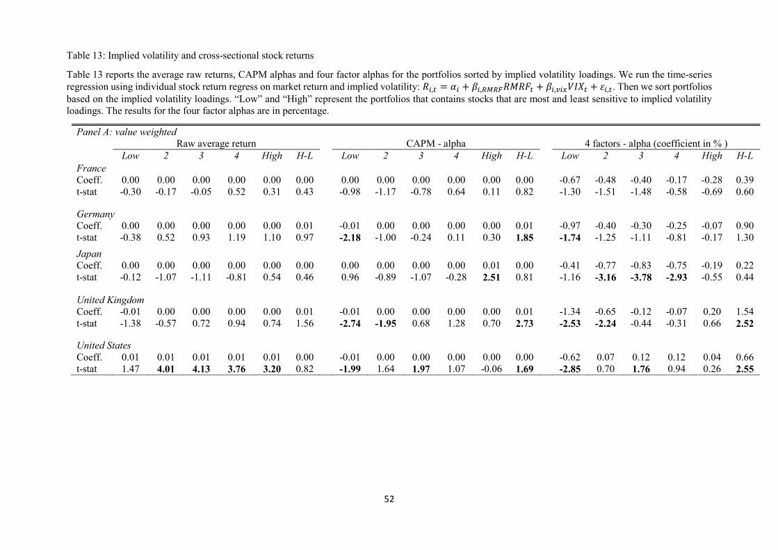
52
Table 13: Implied volatility and cross-sectional stock returns
Table 13 reports the average raw returns, CAPM alphas and four factor alphas for the portfolios sorted by implied volatility loadings. We run the time-series
regression using individual stock return regress on market return and implied volatility: 𝑅𝑖,𝑡 = 𝛼𝑖 + 𝛽𝑖,𝑅𝑀𝑅𝐹𝑅𝑀𝑅𝐹𝑡 + 𝛽𝑖,𝑣𝑖𝑥𝑉𝐼𝑋𝑡 + 𝜀𝑖,𝑡. Then we sort portfolios
based on the implied volatility loadings. “Low” and “High” represent the portfolios that contains stocks that are most and least sensitive to implied volatility
loadings. The results for the four factor alphas are in percentage.
Panel A: value weighted
Raw average return CAPM - alpha 4 factors - alpha (coefficient in % )
Low 2 3 4 High H-L Low 2 3 4 High H-L Low 2 3 4 High H-L
France Coeff. 0.00 0.00 0.00 0.00 0.00 0.00 0.00 0.00 0.00 0.00 0.00 0.00 -0.67 -0.48 -0.40 -0.17 -0.28 0.39
t-stat -0.30 -0.17 -0.05 0.52 0.31 0.43 -0.98 -1.17 -0.78 0.64 0.11 0.82 -1.30 -1.51 -1.48 -0.58 -0.69 0.60
Germany Coeff. 0.00 0.00 0.00 0.00 0.00 0.01 -0.01 0.00 0.00 0.00 0.00 0.01 -0.97 -0.40 -0.30 -0.25 -0.07 0.90
t-stat -0.38 0.52 0.93 1.19 1.10 0.97 -2.18 -1.00 -0.24 0.11 0.30 1.85 -1.74 -1.25 -1.11 -0.81 -0.17 1.30
Japan Coeff. 0.00 0.00 0.00 0.00 0.00 0.00 0.00 0.00 0.00 0.00 0.01 0.00 -0.41 -0.77 -0.83 -0.75 -0.19 0.22
t-stat -0.12 -1.07 -1.11 -0.81 0.54 0.46 0.96 -0.89 -1.07 -0.28 2.51 0.81 -1.16 -3.16 -3.78 -2.93 -0.55 0.44
United Kingdom Coeff. -0.01 0.00 0.00 0.00 0.00 0.01 -0.01 0.00 0.00 0.00 0.00 0.01 -1.34 -0.65 -0.12 -0.07 0.20 1.54
t-stat -1.38 -0.57 0.72 0.94 0.74 1.56 -2.74 -1.95 0.68 1.28 0.70 2.73 -2.53 -2.24 -0.44 -0.31 0.66 2.52
United States Coeff. 0.01 0.01 0.01 0.01 0.01 0.00 -0.01 0.00 0.00 0.00 0.00 0.00 -0.62 0.07 0.12 0.12 0.04 0.66
t-stat 1.47 4.01 4.13 3.76 3.20 0.82 -1.99 1.64 1.97 1.07 -0.06 1.69 -2.85 0.70 1.76 0.94 0.26 2.55

53
Table 13. Continued
Panel B: Equally weighted
Raw average return CAPM - alpha 4 factors - alpha (coefficient in % )
Low 2 3 4 High H-L Low 2 3 4 High H-L Low 2 3 4 High H-L
France Coeff. 0.00 0.00 -0.01 0.00 0.00 0.00 0.00 -0.01 -0.01 -0.01 0.00 0.00 0.22 -0.78 -0.82 -0.76 -0.16 -0.37
t-stat 0.63 -0.96 -1.37 -1.05 0.21 -0.37 -0.58 -2.32 -3.00 -2.37 -0.02 -0.48 0.45 -3.02 -3.78 -2.97 -0.46 -0.63
Germany Coeff. 0.00 0.00 0.00 0.00 0.00 0.00 -0.01 -0.01 -0.01 -0.01 -0.01 0.00 -0.70 -0.85 -0.89 -0.89 -0.72 -0.02
t-stat -0.71 -1.76 -2.34 -1.91 -0.85 -0.10 -2.08 -5.34 -6.50 -5.38 -2.51 -0.17 -1.76 -3.89 -5.17 -4.30 -1.89 -0.04
Japan Coeff. 0.01 0.00 0.00 0.00 0.01 0.00 0.01 0.00 0.00 0.00 0.02 0.00 0.01 -1.19 -1.08 -0.99 0.42 0.41
t-stat 1.43 -1.27 -1.31 0.01 2.19 0.48 2.89 -1.04 -1.13 -0.43 4.05 0.68 0.04 -5.70 -5.82 -4.76 -1.29 0.90
United Kingdom Coeff. 0.00 -0.01 0.00 0.00 0.00 0.00 -0.01 -0.01 -0.01 -0.01 -0.01 0.00 -0.60 -0.87 -0.78 -0.72 -0.57 0.02
t-stat -0.55 -1.37 -1.36 -1.29 -0.72 -0.04 -1.06 -2.82 -3.15 -2.81 -1.44 -0.03 -1.69 -4.21 -4.34 -3.62 -1.89 0.05
United States Coeff. 0.02 0.01 0.01 0.01 0.01 0.00 0.01 0.00 0.00 0.00 0.01 0.00 0.30 -0.16 -0.23 -0.11 0.34 0.04
t-stat 3.81 3.14 2.99 3.19 4.06 -0.27 1.76 0.43 0.14 0.55 2.00 -0.04 1.72 -1.83 -2.90 -1.07 2.22 0.18
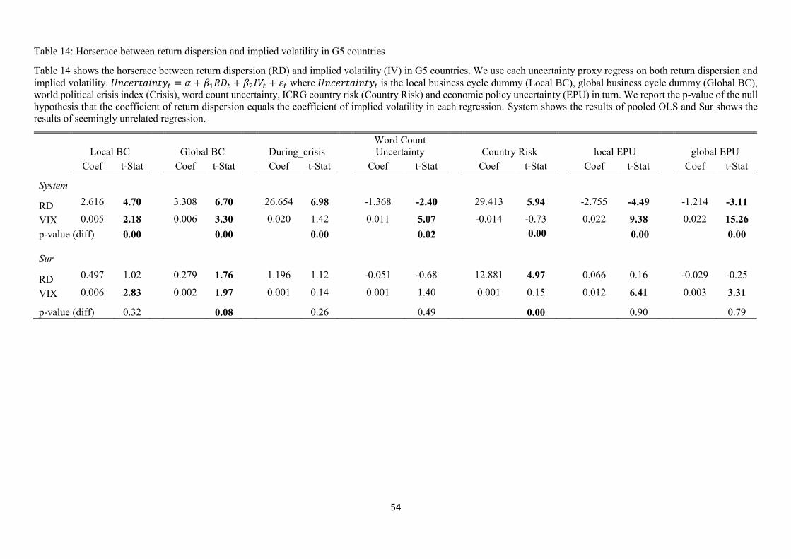
54
Table 14: Horserace between return dispersion and implied volatility in G5 countries
Table 14 shows the horserace between return dispersion (RD) and implied volatility (IV) in G5 countries. We use each uncertainty proxy regress on both return dispersion and
implied volatility. 𝑈𝑛𝑐𝑒𝑟𝑡𝑎𝑖𝑛𝑡𝑦𝑡 = 𝛼 + 𝛽1𝑅𝐷𝑡 + 𝛽2𝐼𝑉𝑡 + 𝜀𝑡 where 𝑈𝑛𝑐𝑒𝑟𝑡𝑎𝑖𝑛𝑡𝑦𝑡 is the local business cycle dummy (Local BC), global business cycle dummy (Global BC),
world political crisis index (Crisis), word count uncertainty, ICRG country risk (Country Risk) and economic policy uncertainty (EPU) in turn. We report the p-value of the null
hypothesis that the coefficient of return dispersion equals the coefficient of implied volatility in each regression. System shows the results of pooled OLS and Sur shows the
results of seemingly unrelated regression.
Local BC Global BC During_crisis
Word Count
Uncertainty Country Risk local EPU global EPU
Coef t-Stat Coef t-Stat Coef t-Stat Coef t-Stat Coef t-Stat Coef t-Stat Coef t-Stat
System
RD 2.616 4.70
3.308 6.70
26.654 6.98
-1.368 -2.40
29.413 5.94
-2.755 -4.49
-1.214 -3.11
VIX 0.005 2.18 0.006 3.30 0.020 1.42 0.011 5.07 -0.014 -0.73 0.022 9.38 0.022 15.26
p-value (diff) 0.00 0.00 0.00 0.02 0.00 0.00 0.00
Sur
RD 0.497 1.02
0.279 1.76
1.196 1.12
-0.051 -0.68
12.881 4.97
0.066 0.16
-0.029 -0.25
VIX 0.006 2.83 0.002 1.97 0.001 0.14 0.001 1.40 0.001 0.15 0.012 6.41 0.003 3.31
p-value (diff) 0.32 0.08 0.26 0.49 0.00 0.90 0.79
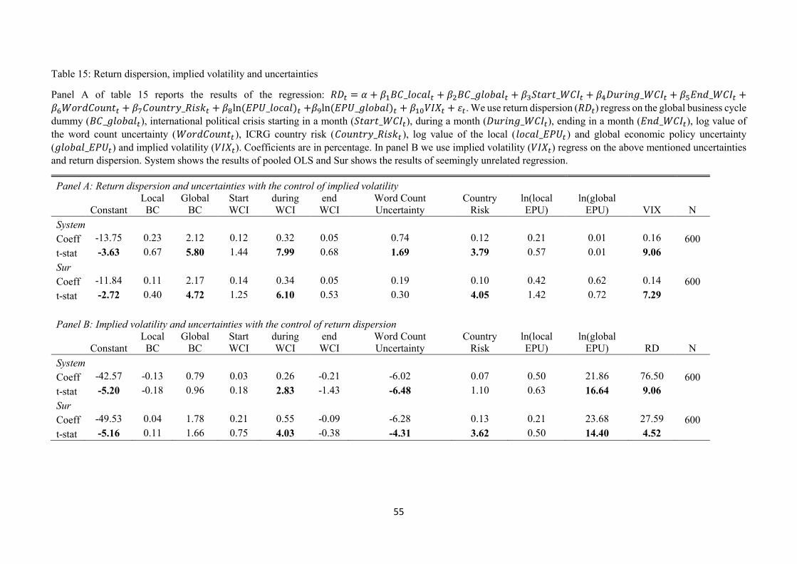
55
Table 15: Return dispersion, implied volatility and uncertainties
Panel A of table 15 reports the results of the regression: 𝑅𝐷𝑡 = 𝛼 + 𝛽1𝐵𝐶_𝑙𝑜𝑐𝑎𝑙𝑡 + 𝛽2𝐵𝐶_𝑔𝑙𝑜𝑏𝑎𝑙𝑡 + 𝛽3𝑆𝑡𝑎𝑟𝑡_𝑊𝐶𝐼𝑡 + 𝛽4𝐷𝑢𝑟𝑖𝑛𝑔_𝑊𝐶𝐼𝑡 + 𝛽5𝐸𝑛𝑑_𝑊𝐶𝐼𝑡 +
𝛽6𝑊𝑜𝑟𝑑𝐶𝑜𝑢𝑛𝑡𝑡 + 𝛽7𝐶𝑜𝑢𝑛𝑡𝑟𝑦_𝑅𝑖𝑠𝑘𝑡 + 𝛽8ln (𝐸𝑃𝑈_𝑙𝑜𝑐𝑎𝑙)𝑡 +𝛽9ln (𝐸𝑃𝑈_𝑔𝑙𝑜𝑏𝑎𝑙)𝑡 + 𝛽10𝑉𝐼𝑋𝑡 + 𝜀𝑡. We use return dispersion (𝑅𝐷𝑡) regress on the global business cycle
dummy (𝐵𝐶_𝑔𝑙𝑜𝑏𝑎𝑙𝑡), international political crisis starting in a month (𝑆𝑡𝑎𝑟𝑡_𝑊𝐶𝐼𝑡), during a month (𝐷𝑢𝑟𝑖𝑛𝑔_𝑊𝐶𝐼𝑡), ending in a month (𝐸𝑛𝑑_𝑊𝐶𝐼𝑡), log value of
the word count uncertainty (𝑊𝑜𝑟𝑑𝐶𝑜𝑢𝑛𝑡𝑡 ), ICRG country risk (𝐶𝑜𝑢𝑛𝑡𝑟𝑦_𝑅𝑖𝑠𝑘𝑡 ), log value of the local (𝑙𝑜𝑐𝑎𝑙_𝐸𝑃𝑈𝑡 ) and global economic policy uncertainty
(𝑔𝑙𝑜𝑏𝑎𝑙_𝐸𝑃𝑈𝑡) and implied volatility (𝑉𝐼𝑋𝑡). Coefficients are in percentage. In panel B we use implied volatility (𝑉𝐼𝑋𝑡) regress on the above mentioned uncertainties
and return dispersion. System shows the results of pooled OLS and Sur shows the results of seemingly unrelated regression.
Panel A: Return dispersion and uncertainties with the control of implied volatility
Constant
Local
BC
Global
BC
Start
WCI
during
WCI
end
WCI
Word Count
Uncertainty
Country
Risk
ln(local
EPU)
ln(global
EPU) VIX N
System Coeff -13.75 0.23 2.12 0.12 0.32 0.05 0.74 0.12 0.21 0.01 0.16 600
t-stat -3.63 0.67 5.80 1.44 7.99 0.68 1.69 3.79 0.57 0.01 9.06 Sur Coeff -11.84 0.11 2.17 0.14 0.34 0.05 0.19 0.10 0.42 0.62 0.14 600
t-stat -2.72 0.40 4.72 1.25 6.10 0.53 0.30 4.05 1.42 0.72 7.29
Panel B: Implied volatility and uncertainties with the control of return dispersion
Constant
Local
BC
Global
BC
Start
WCI
during
WCI
end
WCI
Word Count
Uncertainty
Country
Risk
ln(local
EPU)
ln(global
EPU) RD N
System Coeff -42.57 -0.13 0.79 0.03 0.26 -0.21 -6.02 0.07 0.50 21.86 76.50 600
t-stat -5.20 -0.18 0.96 0.18 2.83 -1.43 -6.48 1.10 0.63 16.64 9.06 Sur Coeff -49.53 0.04 1.78 0.21 0.55 -0.09 -6.28 0.13 0.21 23.68 27.59 600
t-stat -5.16 0.11 1.66 0.75 4.03 -0.38 -4.31 3.62 0.50 14.40 4.52

56
Figure 1: Return dispersion of all stocks versus return dispersion of the largest (market capitalization) 50 stocks in the US
Figure 1 plots two return dispersion indices in the US stock market. The dashed line (RDUSA) is the return dispersion made by all available US stocks. The solid line
is the return dispersion computed using 50 largest (market capitalization) stocks.
0
0.05
0.1
0.15
0.2
0.25
19
86
M0
1
19
87
M0
1
19
88
M0
1
19
89
M0
1
19
90
M0
1
19
91
M0
1
19
92
M0
1
19
93
M0
1
19
94
M0
1
19
95
M0
1
19
96
M0
1
19
97
M0
1
19
98
M0
1
19
99
M0
1
20
00
M0
1
20
01
M0
1
20
02
M0
1
20
03
M0
1
20
04
M0
1
20
05
M0
1
20
06
M0
1
20
07
M0
1
20
08
M0
1
20
09
M0
1
20
10
M0
1
20
11
M0
1
20
12
M0
1
20
13
M0
1
RDUSARD50USA

57
Figure 2: Return dispersion in US and events
Figure 2 plots the return dispersion of the largest 50 US stocks from January 1986 to December 2013. The shaded areas are NBER recessions.

58
Figure 3a: Four-factor alphas of value-weighted portfolios sorted by return dispersion betas
Low Group 2Group 3 Group 4
High
-5.00
-4.00
-3.00
-2.00
-1.00
0.00
1.00
2.00
3.00
4.00
AustraliaBelgium
FranceGermany
ItalyJapan
NetherlandNorway
SpainSwedenSwitzerland
UK
US
59
Figure 4b: Four-factor alphas of equal-weighted portfolios sorted by return dispersion betas
Low Group 2 Group 3 Group 4High
-2.50
-2.00
-1.50
-1.00
-0.50
0.00
0.50
1.00
1.50
2.00
AustraliaBelgium
FranceGermany
ItalyJapan
NetherlandNorway
SpainSwedenSwitzerland
UK
US

60
Figure 5: Return dispersion and implied volatility
Figure 4 plots the return dispersion and its contemporaneous implied volatility index for each country. The return dispersion is calculated using the largest 50 stock
returns. The implied volatility indices we use include CAC40 Volatility Index (France), VDAX New Volatility Index (Germany), NIKKEI Stock Average Volatility
Index (Japan), FTSE 100 Volatility Index (UK) and CBOE SPX Volatility VIX (US).
0
0.05
0.1
0.15
0.2
0.25
0
10
20
30
40
50
60
2000 2001 2002 2003 2004 2005 2006 2007 2008 2009 2010 2011 2012 2013
France
Implied Volatility Return Dispersion
0
10
20
30
40
50
60
70
0
0.05
0.1
0.15
0.2
0.25
0.3
1992 1993 1995 1996 1998 1999 2001 2002 2004 2005 2007 2008 2010 2011 2013
Germany
Return Dispersion Implied Volatility

61
Figure 5. Continued
0
0.05
0.1
0.15
0.2
0.25
0.3
0
10
20
30
40
50
60
70
80
1998 1999 2001 2002 2004 2005 2007 2008 2010 2011 2013
Japan
Implied Volatility Return Dispersion
0
10
20
30
40
50
0
0.05
0.1
0.15
0.2
0.25
2000 2001 2003 2004 2006 2007 2009 2010 2012 2013
UK
Return Dispersion Implied Volatility
0
10
20
30
40
50
60
70
0
0.05
0.1
0.15
0.2
0.25
1990 1992 1994 1996 1998 2000 2002 2004 2006 2008 2010 2012
US
Return Dispersion Implied Volatility
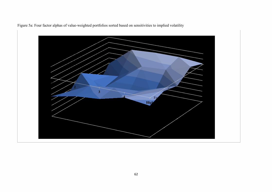
62
Figure 5a: Four factor alphas of value-weighted portfolios sorted based on sensitivities to implied volatility
France
Germany
Japan
UK
US
-1.40
-1.20
-1.00
-0.80
-0.60
-0.40
-0.20
0.00
0.20
0.40
Low
2
3
4
High

63
Figure 5b: Four factor alphas of equal-weighted portfolios sorted based on sensitivities to implied volatility
France
Germany
Japan
United Kingdom
United States
-1.20
-1.00
-0.80
-0.60
-0.40
-0.20
0.00
0.20
0.40
0.60
Low
2
3
4
High
64
Appendix A A1. Correlations of uncertainty variables in each country
This table shows the correlations across all variables in each country (shown in separate panels).
Panel A: Australia
RD Local BC Global BC
Start
WCI During WCI
End
WCI
Word
Count
Country
Risk
ln(local
EPU)
ln(global
EPU)
RD 1.00
Local BC 0.37 1.00
Global BC 0.47 0.63 1.00
Start WCI 0.05 -0.13 -0.10 1.00
During WCI -0.03 -0.01 -0.10 0.04 1.00
End WCI 0.09 -0.04 -0.04 0.09 0.01 1.00
Word Count 0.28 0.28 0.35 -0.14 -0.15 -0.15 1.00
Country Risk -0.27 -0.20 -0.36 -0.10 -0.18 0.04 -0.04 1.00
ln(local EPU) 0.51 0.23 0.36 0.12 0.15 0.02 0.41 -0.42 1.00 ln(global EPU) 0.42 0.30 0.36 0.11 0.02 0.04 0.47 -0.44 0.84 1.00
Panel B: Austria
RD Local BC Global BC
Start
WCI During WCI
End
WCI
Word
Count
Country
Risk
ln(global
EPU)
RD 1.00
Local BC 0.49 1.00
Global BC 0.43 0.60 1.00
Start WCI -0.01 -0.04 -0.08 1.00
During WCI 0.10 -0.02 -0.07 0.05 1.00
End WCI 0.12 -0.01 -0.03 0.09 0.02 1.00
Word Count 0.35 0.25 0.35 -0.06 0.01 -0.08 1.00
Country Risk -0.19 -0.37 -0.24 0.07 -0.21 0.02 -0.30 1.00 ln(global EPU) 0.48 0.29 0.36 0.13 0.05 0.04 0.42 0.12 1.00
65
Panel C: Belgium
RD Local BC Global BC
Start
WCI During WCI
End
WCI
Word
Count
Country
Risk
ln(global
EPU)
RD 1.00
Local BC 0.34 1.00
Global BC 0.50 0.40 1.00
Start WCI 0.04 -0.19 -0.08 1.00
During WCI 0.15 0.15 -0.07 0.05 1.00
End WCI 0.11 -0.10 -0.03 0.09 0.02 1.00
Word Count 0.30 0.11 0.35 -0.06 0.01 -0.08 1.00
Country Risk -0.40 -0.51 -0.27 0.02 -0.46 -0.02 -0.04 1.00
ln(global EPU) 0.55 0.12 0.36 0.13 0.05 0.04 0.42 -0.05 1.00
Panel D: Denmark
RD Local BC Global BC
Start
WCI During WCI
End
WCI
Word
Count
Country
Risk
ln(global
EPU)
RD 1.00
Local BC 0.29 1.00
Global BC 0.46 0.38 1.00
Start WCI -0.01 -0.14 -0.08 1.00
During WCI 0.17 -0.27 -0.07 0.05 1.00
End WCI -0.07 -0.06 -0.03 0.09 0.02 1.00
Word Count 0.29 0.24 0.35 -0.06 0.01 -0.08 1.00
Country Risk -0.10 0.01 -0.09 0.06 -0.02 -0.01 -0.17 1.00
ln(global EPU) 0.44 0.28 0.36 0.13 0.05 0.04 0.42 0.07 1.00
66
Panel E: Finland
RD Local BC Global BC
Start
WCI During WCI
End
WCI
Word
Count
Country
Risk
ln(global
EPU)
RD 1.00
Local BC 0.29 1.00
Global BC 0.41 0.56 1.00
Start WCI 0.03 -0.02 -0.08 1.00
During WCI 0.35 -0.12 -0.07 0.05 1.00
End WCI -0.04 0.00 -0.03 0.09 0.02 1.00
Word Count 0.28 0.26 0.35 -0.06 0.01 -0.08 1.00
Country Risk 0.14 0.16 -0.03 0.07 0.04 0.06 0.13 1.00
ln(global EPU) 0.38 0.29 0.36 0.13 0.05 0.04 0.42 0.02 1.00
Panel F: France
RD Local BC Global BC
Start
WCI During WCI
End
WCI
Word
Count
Country
Risk
ln(local
EPU)
ln(global
EPU) VIX
RD 1.00
Local BC 0.41 1.00
Global BC 0.32 0.53 1.00
Start WCI 0.14 -0.02 -0.08 1.00
During WCI 0.42 0.32 0.00 -0.06 1.00
End WCI 0.03 0.01 -0.02 0.20 -0.09 1.00
Word Count 0.27 0.36 0.33 -0.07 0.17 -0.10 1.00
Country Risk 0.40 0.46 -0.02 0.01 0.32 0.04 0.19 1.00
ln(local EPU) 0.04 -0.33 0.01 0.12 -0.32 0.01 0.23 -0.20 1.00
ln(global EPU) 0.55 0.31 0.38 0.10 0.08 0.05 0.61 0.26 0.54 1.00
VIX 0.77 0.18 0.24 0.15 0.29 0.06 0.32 0.30 0.37 0.77 1.00

67
Panel G: Germany
RD Local BC Global BC
Start
WCI During WCI
End
WCI
Word
Count
Country
Risk
ln(local
EPU)
ln(global
EPU) VIX
RD 1.00
Local BC 0.38 1.00
Global BC 0.46 0.60 1.00
Start WCI 0.02 -0.01 -0.08 1.00
During WCI 0.22 -0.13 -0.07 0.05 1.00
End WCI 0.02 0.04 -0.03 0.09 0.02 1.00
Word Count 0.31 0.16 0.35 -0.06 0.01 -0.08 1.00
Country Risk 0.16 0.41 0.30 0.04 0.14 0.04 -0.02 1.00
ln(local EPU) 0.46 0.22 0.21 0.11 0.16 0.02 0.40 0.14 1.00
ln(global EPU) 0.60 0.31 0.36 0.13 0.05 0.04 0.42 0.09 0.67 1.00
VIX 0.66 0.24 0.15 0.14 0.26 0.05 0.16 -0.01 0.52 0.73 1.00
Panel H: Ireland
RD Local BC Global BC
Start
WCI During WCI
End
WCI
Word
Count
Country
Risk
ln(local
EPU)
ln(global
EPU)
RD 1.00
Local BC 0.38 1.00
Global BC 0.40 0.37 1.00
Start WCI 0.07 -0.02 -0.08 1.00
During WCI 0.02 -0.06 -0.07 0.05 1.00
End WCI 0.01 0.03 -0.03 0.09 0.02 1.00
Word Count 0.33 0.27 0.35 -0.06 0.01 -0.08 1.00
Country Risk -0.24 -0.21 -0.24 0.09 0.11 0.09 -0.28 1.00
ln(local EPU) 0.31 0.17 0.18 -0.16 -0.08 0.06 0.18 -0.24 1.00
ln(global EPU) 0.43 0.26 0.36 0.13 0.05 0.04 0.42 -0.06 0.42 1.00

68
Panel I: Italy
RD Local BC Global BC
Start
WCI During WCI
End
WCI
Word
Count
Country
Risk
ln(local
EPU)
ln(global
EPU)
RD 1.00
Local BC 0.14 1.00
Global BC 0.14 0.63 1.00
Start WCI 0.00 -0.03 -0.08 1.00
During WCI 0.13 -0.14 -0.07 0.05 1.00
End WCI 0.04 0.02 -0.03 0.09 0.02 1.00
Word Count 0.03 0.18 0.35 -0.06 0.01 -0.08 1.00
Country Risk 0.08 -0.21 -0.17 0.11 0.02 0.03 -0.33 1.00
ln(local EPU) 0.24 -0.05 -0.03 0.02 0.04 0.02 0.06 0.41 1.00
ln(global EPU) 0.27 0.35 0.36 0.13 0.05 0.04 0.42 0.18 0.55 1.00
Panel J: Japan
RD Local BC Global BC
Start
WCI During WCI
End
WCI
Word
Count
Country
Risk
ln(local
EPU)
ln(global
EPU) VIX
RD 1.00
Local BC 0.08 1.00
Global BC 0.22 0.58 1.00
Start WCI -0.01 0.07 -0.10 1.00
During WCI 0.40 -0.15 -0.10 0.04 1.00
End WCI -0.03 0.00 -0.04 0.09 0.01 1.00
Word Count 0.15 0.11 0.35 -0.14 -0.15 -0.15 1.00
Country Risk -0.17 -0.12 -0.21 -0.05 -0.30 -0.03 -0.05 1.00
ln(local EPU) 0.21 0.31 0.18 0.06 0.11 0.08 0.18 -0.39 1.00
ln(global EPU) 0.16 0.38 0.36 0.11 0.02 0.04 0.47 -0.16 0.63 1.00
VIX 0.31 0.42 0.45 0.04 0.02 -0.03 0.26 -0.23 0.45 0.73 1.00

69
Panel K: Netherlands
RD Local BC Global BC
Start
WCI During WCI
End
WCI
Word
Count
Country
Risk
ln(local
EPU)
ln(global
EPU)
RD 1.00
Local BC 0.65 1.00
Global BC 0.60 0.77 1.00
Start WCI -0.03 0.02 0.04 1.00
During WCI 0.03 -0.07 0.00 -0.07 1.00
End WCI -0.11 0.04 0.01 0.09 -0.06 1.00
Word Count 0.31 0.31 0.27 -0.11 0.08 -0.11 1.00
Country Risk -0.05 0.01 0.11 0.04 -0.31 -0.03 -0.22 1.00
ln(local EPU) 0.52 0.60 0.43 -0.03 -0.05 -0.08 0.52 -0.32 1.00
ln(global EPU) 0.67 0.61 0.58 -0.04 0.03 -0.05 0.65 -0.08 0.73 1.00
Panel L: Norway
RD Local BC Global BC
Start
WCI During WCI
End
WCI
Word
Count
Country
Risk
ln(global
EPU)
RD 1.00
Local BC 0.26 1.00
Global BC 0.29 0.20 1.00
Start WCI 0.12 0.06 -0.08 1.00
During WCI 0.29 0.02 -0.07 0.05 1.00
End WCI 0.05 0.07 -0.03 0.09 0.02 1.00
Word Count 0.41 0.24 0.35 -0.06 0.01 -0.08 1.00
Country Risk -0.13 -0.09 -0.13 0.06 -0.54 0.02 -0.03 1.00
ln(global EPU) 0.61 0.44 0.36 0.13 0.05 0.04 0.42 -0.04 1.00
70
Panel M: New Zealand
RD Local BC Global BC
Start
WCI During WCI
End
WCI
Word
Count
Country
Risk
ln(global
EPU)
RD 1.00
Local BC -0.02 1.00
Global BC 0.26 -0.01 1.00
Start WCI 0.08 -0.11 -0.08 1.00
During WCI 0.26 -0.02 -0.07 0.05 1.00
End WCI 0.01 -0.11 -0.03 0.09 0.02 1.00
Word Count 0.25 -0.24 0.35 -0.06 0.01 -0.08 1.00
Country Risk -0.32 0.21 -0.40 -0.15 -0.39 -0.07 -0.38 1.00
ln(global EPU) 0.34 -0.14 0.36 0.13 0.05 0.04 0.42 -0.30 1.00
Panel N: Spain
RD Local BC Global BC
Start
WCI During WCI
End
WCI
Word
Count
Country
Risk
ln(local
EPU)
ln(global
EPU)
RD 1.00
Local BC 0.49 1.00
Global BC 0.47 0.66 1.00
Start WCI 0.11 0.01 -0.06 1.00
During WCI 0.20 -0.11 -0.06 0.04 1.00
End WCI 0.11 0.01 -0.06 0.21 -0.03 1.00
Word Count 0.25 0.20 0.32 -0.06 0.17 -0.12 1.00
Country Risk -0.36 -0.49 -0.35 0.08 0.06 0.10 -0.19 1.00
ln(local EPU) 0.17 0.09 0.02 0.11 0.18 0.06 0.40 0.24 1.00
ln(global EPU) 0.50 0.40 0.41 0.08 0.25 0.01 0.64 -0.12 0.71 1.00
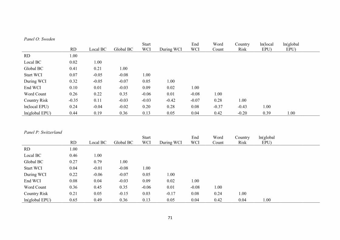
71
Panel O: Sweden
RD Local BC Global BC
Start
WCI During WCI
End
WCI
Word
Count
Country
Risk
ln(local
EPU)
ln(global
EPU)
RD 1.00
Local BC 0.02 1.00
Global BC 0.41 0.21 1.00
Start WCI 0.07 -0.05 -0.08 1.00
During WCI 0.32 -0.05 -0.07 0.05 1.00
End WCI 0.10 0.01 -0.03 0.09 0.02 1.00
Word Count 0.26 0.22 0.35 -0.06 0.01 -0.08 1.00
Country Risk -0.35 0.11 -0.03 -0.03 -0.42 -0.07 0.28 1.00
ln(local EPU) 0.24 -0.04 -0.02 0.20 0.28 0.08 -0.37 -0.43 1.00
ln(global EPU) 0.44 0.19 0.36 0.13 0.05 0.04 0.42 -0.20 0.39 1.00
Panel P: Switzerland
RD Local BC Global BC
Start
WCI During WCI
End
WCI
Word
Count
Country
Risk
ln(global
EPU)
RD 1.00
Local BC 0.46 1.00
Global BC 0.27 0.79 1.00
Start WCI 0.04 -0.01 -0.08 1.00
During WCI 0.22 -0.06 -0.07 0.05 1.00
End WCI 0.08 0.04 -0.03 0.09 0.02 1.00
Word Count 0.36 0.45 0.35 -0.06 0.01 -0.08 1.00
Country Risk 0.21 0.05 -0.15 0.03 -0.17 0.08 0.24 1.00
ln(global EPU) 0.65 0.49 0.36 0.13 0.05 0.04 0.42 0.04 1.00
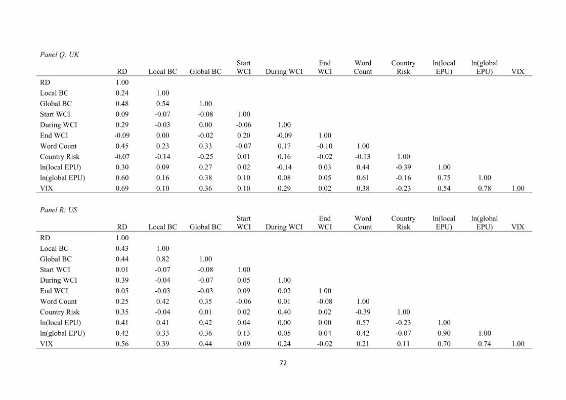
72
Panel Q: UK
RD Local BC Global BC
Start
WCI During WCI
End
WCI
Word
Count
Country
Risk
ln(local
EPU)
ln(global
EPU) VIX
RD 1.00
Local BC 0.24 1.00
Global BC 0.48 0.54 1.00
Start WCI 0.09 -0.07 -0.08 1.00
During WCI 0.29 -0.03 0.00 -0.06 1.00
End WCI -0.09 0.00 -0.02 0.20 -0.09 1.00
Word Count 0.45 0.23 0.33 -0.07 0.17 -0.10 1.00
Country Risk -0.07 -0.14 -0.25 0.01 0.16 -0.02 -0.13 1.00
ln(local EPU) 0.30 0.09 0.27 0.02 -0.14 0.03 0.44 -0.39 1.00
ln(global EPU) 0.60 0.16 0.38 0.10 0.08 0.05 0.61 -0.16 0.75 1.00
VIX 0.69 0.10 0.36 0.10 0.29 0.02 0.38 -0.23 0.54 0.78 1.00
Panel R: US
RD Local BC Global BC
Start
WCI During WCI
End
WCI
Word
Count
Country
Risk
ln(local
EPU)
ln(global
EPU) VIX
RD 1.00
Local BC 0.43 1.00
Global BC 0.44 0.82 1.00
Start WCI 0.01 -0.07 -0.08 1.00
During WCI 0.39 -0.04 -0.07 0.05 1.00
End WCI 0.05 -0.03 -0.03 0.09 0.02 1.00
Word Count 0.25 0.42 0.35 -0.06 0.01 -0.08 1.00
Country Risk 0.35 -0.04 0.01 0.02 0.40 0.02 -0.39 1.00
ln(local EPU) 0.41 0.41 0.42 0.04 0.00 0.00 0.57 -0.23 1.00
ln(global EPU) 0.42 0.33 0.36 0.13 0.05 0.04 0.42 -0.07 0.90 1.00
VIX 0.56 0.39 0.44 0.09 0.24 -0.02 0.21 0.11 0.70 0.74 1.00

73
A2. Return dispersion and number of crisis starting in a month (Crisis start), during a month (Crisis during), and ending in a month (Crisis end).
This table shows the results of return dispersion regress on international political crisis with the control of business cycle in each country (𝑅𝐷𝑡 = 𝛼 + 𝛽1𝐵𝐶_𝑙𝑜𝑐𝑎𝑙𝑡 +𝛽2𝐵𝐶_𝑔𝑙𝑜𝑏𝑎𝑙𝑡 + 𝛽3𝐶𝑟𝑖𝑠𝑖𝑠_𝑠𝑡𝑎𝑟𝑡𝑡 + 𝛽4𝐶𝑟𝑖𝑠𝑖𝑠_𝑑𝑢𝑟𝑖𝑛𝑔𝑡 + 𝛽5𝐶𝑟𝑖𝑠𝑖𝑠_𝑒𝑛𝑑𝑡 + 𝜀𝑡). 𝑅𝐷𝑡 is the return dispersion of the largest 50 market capitalization stocks in each
country at time t. 𝐵𝐶_𝑙𝑜𝑐𝑎𝑙𝑡 and 𝐵𝐶_𝑔𝑙𝑜𝑏𝑎𝑙𝑡 are the dummy variables for business cycle (1= recession, 0 = expansion) in local country and global respectively.
𝐶𝑟𝑖𝑠𝑖𝑠_𝑠𝑡𝑎𝑟𝑡𝑡, 𝐶𝑟𝑖𝑠𝑖𝑠_𝑑𝑢𝑟𝑖𝑛𝑔𝑡 and 𝐶𝑟𝑖𝑠𝑖𝑠_𝑒𝑛𝑑𝑡 are numbers of crisis starting at month t, during month t and ending at month t. System shows the results of pooled
OLS and Sur shows the results of seemingly unrelated regression. We use robust standard errors. Coefficients are in percentage.
Constant t-value
Local
BC t-value
Global
BC t-value
Crisis
start t-value
Crisis
during t-value
Crisis
End t-value
Adjusted
R2
Australia 6.45 20.68 0.43 0.65 4.24 4.20 0.40 1.33 0.17 0.84 0.54 1.59 0.10
Austria 8.04 20.04 1.97 2.68 5.11 4.06 -0.26 -0.84 -0.03 -0.21 0.59 1.00 0.18
Belgium 6.17 16.71 0.21 0.48 5.77 5.55 -0.02 -0.06 0.02 0.13 0.30 0.96 0.21
Denmark 7.28 27.31 0.10 0.22 6.76 4.35 0.06 0.19 0.31 2.39 -0.44 -1.69 0.22
Finland 7.38 20.56 2.14 3.24 3.57 3.36 0.39 1.33 0.72 4.30 0.22 0.80 0.17
France 5.91 25.39 1.37 3.80 2.16 3.27 0.11 0.38 0.22 1.70 0.08 0.25 0.13
Germany 6.76 25.13 -0.11 -0.12 5.78 6.07 0.07 0.23 -0.06 -0.47 -0.03 -0.09 0.23
Ireland 7.59 15.15 3.85 4.81 5.71 3.58 0.68 1.21 0.94 3.54 -0.07 -0.15 0.22
Italy 7.37 16.06 1.27 2.13 1.33 2.26 -0.36 -1.17 -0.08 -0.39 0.18 0.53 0.02
Japan 6.88 18.57 -0.05 -0.10 3.23 4.71 0.53 1.44 0.21 1.20 -0.09 -0.29 0.05
Netherlands 6.74 18.10 3.72 3.46 1.56 1.39 0.32 0.73 0.12 0.70 -0.20 -0.47 0.16
Norge 9.58 16.41 2.06 2.27 3.50 3.46 0.20 0.46 0.20 0.86 -0.25 -0.64 0.06
New Zealand 7.92 15.97 0.00 0.00 1.12 1.58 1.09 1.76 0.76 3.50 -0.06 -0.16 0.04
Spain 6.07 20.76 1.06 1.93 2.55 2.89 0.99 2.57 0.48 2.89 0.82 2.42 0.13
Sweden 6.22 23.83 -0.77 -2.24 4.05 6.65 0.51 1.47 0.74 5.17 0.42 1.29 0.19
Switzerland 6.23 25.01 3.08 2.00 1.03 0.62 -0.08 -0.33 0.13 1.07 0.29 0.96 0.15
UK 6.29 22.04 -0.61 -1.94 5.49 6.14 0.57 2.23 0.13 1.18 -0.54 -2.20 0.23
US 5.88 28.03 0.93 1.85 4.27 4.97 -0.11 -0.54 0.20 1.99 -0.03 -0.15 0.24
System 6.92 68.85 0.84 5.86 4.01 19.89 0.28 3.07 0.30 6.59 0.11 1.26
Sur 6.70 32.75 0.40 4.34 4.00 10.17 0.18 0.95 0.35 3.63 0.27 1.60
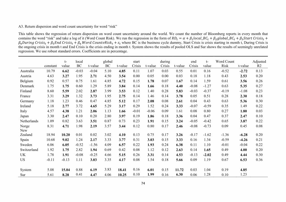
74
A3. Return dispersion and word count uncertainty for word “risk”
This table shows the regression of return dispersion on word count uncertainty around the world. We count the number of Bloomberg reports in every month that
contains the word “risk” and take a log of it (Word Count Risk). We run the regression in the form of 𝑅𝐷𝑡 = 𝛼 + 𝛽1𝑙𝑜𝑐𝑎𝑙_𝐵𝐶𝑡 + 𝛽2𝑔𝑙𝑜𝑏𝑎𝑙_𝐵𝐶𝑡 + 𝛽3𝑆𝑡𝑎𝑟𝑡 𝐶𝑟𝑖𝑠𝑖𝑠𝑡 +𝛽4𝐷𝑢𝑟𝑖𝑛𝑔 𝐶𝑟𝑖𝑠𝑖𝑠𝑡 + 𝛽5𝐸𝑛𝑑 𝐶𝑟𝑖𝑠𝑖𝑠𝑡 + 𝛽6 𝑊𝑜𝑟𝑑 𝐶𝑜𝑢𝑛𝑡𝑣𝑅𝑖𝑠𝑘𝑡 + 𝜀𝑡 where BC is the business cycle dummy, Start Crisis is crisis starting in month t, During Crisis is
the ongoing crisis in month t and End Crisis is the crisis ending in month t. System shows the results of pooled OLS and Sur shows the results of seemingly unrelated
regression. We use robust standard errors. Coefficients are in percentage.
constant
t-
value
local
BC t-value
global
BC t-value
start
Crisis t-value
during
Crisis t-value
end
Crisis
t-
value
Word Count
Risk t-value
Adjusted
R2
Australia 10.79 6.62 -0.03 -0.04 5.10 4.85 0.11 1.07 0.03 0.55 0.01 0.16 -0.52 -2.72 0.13
Austria 4.63 3.27 1.95 2.71 4.50 3.54 0.00 0.05 0.00 0.03 0.18 1.18 0.43 2.53 0.20
Belgium 0.92 0.57 0.75 1.61 4.85 4.72 0.15 1.78 0.07 1.67 0.14 1.59 0.61 3.56 0.26
Denmark 1.75 1.75 0.60 1.29 5.89 3.84 0.14 1.66 0.18 4.40 -0.08 -1.27 0.63 5.35 0.27
Finland 8.60 5.59 2.02 2.87 3.99 3.53 0.12 1.40 0.28 5.83 -0.03 -0.37 -0.19 -1.08 0.23
France 3.31 3.29 1.32 3.73 1.95 2.75 0.14 1.46 0.14 3.78 0.05 0.51 0.28 2.30 0.18
Germany 1.18 1.23 0.46 0.47 4.85 5.12 0.17 2.08 0.08 2.61 0.04 0.43 0.63 5.36 0.30
Ireland 5.18 2.77 3.72 4.65 5.29 3.17 0.29 1.52 0.24 3.33 -0.07 -0.59 0.35 1.49 0.22
Italy 4.57 4.38 1.21 2.06 1.13 1.66 -0.01 -0.06 0.09 1.61 0.08 0.80 0.27 1.80 0.03
Japan 3.30 2.47 0.10 0.20 2.80 3.97 0.19 1.86 0.18 3.36 0.04 0.47 0.37 2.47 0.10
Netherlands 1.09 0.82 3.63 3.51 0.87 0.73 0.23 1.91 0.15 3.24 -0.05 -0.42 0.65 3.87 0.22
Norge 8.31 4.71 1.98 2.19 3.57 3.44 0.12 0.80 0.17 2.46 -0.08 -0.73 0.09 0.45 0.08
New
Zealand 18.94 10.20 0.01 0.02 3.02 4.10 0.13 0.75 0.17 3.26 -0.17 -1.62 -1.36 -6.28 0.20
Spain 10.68 9.02 1.24 2.17 3.33 3.77 0.31 3.03 0.15 3.33 0.16 1.34 -0.59 -4.26 0.21
Sweden 6.06 6.05 -0.52 -1.56 4.09 6.57 0.22 1.93 0.24 6.38 0.11 1.10 -0.01 -0.04 0.22
Switzerland 1.92 1.75 2.82 1.94 0.69 0.42 0.08 1.12 0.12 2.63 0.14 1.65 0.49 4.00 0.20
UK 1.78 1.91 -0.08 -0.25 4.66 5.15 0.26 3.31 0.14 4.53 -0.13 -2.02 0.49 4.44 0.30
US -0.11 -0.13 1.11 3.03 3.35 4.17 0.08 1.54 0.18 5.66 0.09 1.19 0.67 6.53 0.36
System 5.08 15.04 0.88 6.19 3.83 18.41 0.16 6.01 0.15 11.72 0.03 1.04 0.19 4.85 Sur 5.61 8.28 0.41 4.47 4.06 10.25 0.10 1.99 0.16 6.30 0.06 1.28 0.10 1.23
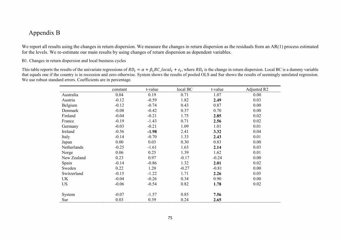
75
Appendix B
We report all results using the changes in return dispersion. We measure the changes in return dispersion as the residuals from an AR(1) process estimated
for the levels. We re-estimate our main results by using changes of return dispersion as dependent variables.
B1. Changes in return dispersion and local business cycles
This table reports the results of the univariate regressions of 𝑅𝐷𝑡 = 𝛼 + 𝛽1𝐵𝐶_𝑙𝑜𝑐𝑎𝑙𝑡 + 𝜀𝑡, where 𝑅𝐷𝑡 is the change in return dispersion. Local BC is a dummy variable
that equals one if the country is in recession and zero otherwise. System shows the results of pooled OLS and Sur shows the results of seemingly unrelated regression.
We use robust standard errors. Coefficients are in percentage.
constant t-value local BC t-value Adjusted R2
Australia 0.04 0.19 0.71 1.07 0.00
Austria -0.12 -0.59 1.82 2.49 0.03
Belgium -0.12 -0.74 0.43 0.87 0.00
Denmark -0.08 -0.42 0.37 0.70 0.00
Finland -0.04 -0.21 1.75 2.85 0.02
France -0.19 -1.43 0.71 2.56 0.02
Germany -0.03 -0.21 1.09 1.01 0.01
Ireland -0.56 -1.98 2.41 3.32 0.04
Italy -0.14 -0.70 1.33 2.43 0.01
Japan 0.00 0.03 0.30 0.83 0.00
Netherlands -0.25 -1.61 1.63 2.14 0.03
Norge 0.06 0.25 1.39 1.62 0.01
New Zealand 0.23 0.97 -0.17 -0.24 0.00
Spain -0.14 -0.86 1.32 2.01 0.02
Sweden 0.22 1.20 -0.27 -0.81 0.00
Switzerland -0.15 -1.22 1.71 2.26 0.05
UK -0.04 -0.26 0.34 0.90 0.00
US -0.06 -0.54 0.82 1.78 0.02
System -0.07 -1.57 0.85 7.56 Sur 0.03 0.39 0.24 2.65

76
B2: Changes in return dispersion and global business cycles
This table reports the coefficients estimates and t-statistics of the regression in the form of 𝑅𝐷𝑡 = 𝛼 + 𝛽1𝑙𝑜𝑐𝑎𝑙 𝐵𝐶𝑡 + 𝛽2𝑔l𝑜𝑏𝑎𝑙 𝐵𝐶𝑡 + 𝜀𝑡, where 𝑅𝐷𝑡 is the change in
return dispersion at time t, 𝑙𝑜𝑐𝑎𝑙 𝐵𝐶𝑡 and 𝑔𝑙𝑜𝑏𝑎𝑙 𝐵𝐶𝑡 are the contemporaneous dummy variable for business cycle (1= recession, 0 = expansion) in local country and
global respectively. System shows the results of pooled OLS and Sur shows the results of seemingly unrelated regression. We use robust standard errors. Coefficients
are in percentage.
constant t-value local BC t-value global BC t-value
Adjusted
R2
Australia -0.05 -0.28 0.22 0.41 1.78 1.95 0.02
Austria -0.23 -1.10 0.90 1.42 2.92 2.82 0.07
Belgium -0.26 -1.53 -0.02 -0.04 2.90 3.26 0.07
Denmark -0.27 -1.34 0.00 0.00 3.81 2.65 0.09
Finland -0.13 -0.71 1.22 1.75 1.85 1.88 0.04
France -0.21 -1.54 0.55 1.88 0.85 1.39 0.03
Germany -0.13 -1.05 0.28 0.34 2.02 2.31 0.05
Ireland -0.64 -2.21 1.69 2.41 2.86 2.52 0.06
Italy -0.20 -0.93 0.94 1.73 1.06 2.23 0.01
Japan -0.02 -0.13 0.02 0.05 1.01 1.69 0.00
Netherlands -0.27 -1.72 1.33 1.55 0.98 0.88 0.04
Norge -0.05 -0.21 1.10 1.39 1.75 1.87 0.02
New Zealand 0.21 0.82 -0.18 -0.25 0.34 0.47 -0.01
Spain -0.17 -1.01 0.88 1.33 1.13 1.26 0.03
Sweden 0.13 0.69 -0.50 -1.53 1.82 3.46 0.03
Switzerland -0.15 -1.22 1.35 0.94 0.69 0.45 0.05
UK -0.09 -0.61 -0.18 -0.72 2.21 2.36 0.05
US -0.06 -0.53 0.18 0.47 1.21 1.44 0.03
System -0.14 -3.05 0.40 3.40 1.85 11.12 Sur -0.09 -1.18 0.12 1.31 1.71 6.20
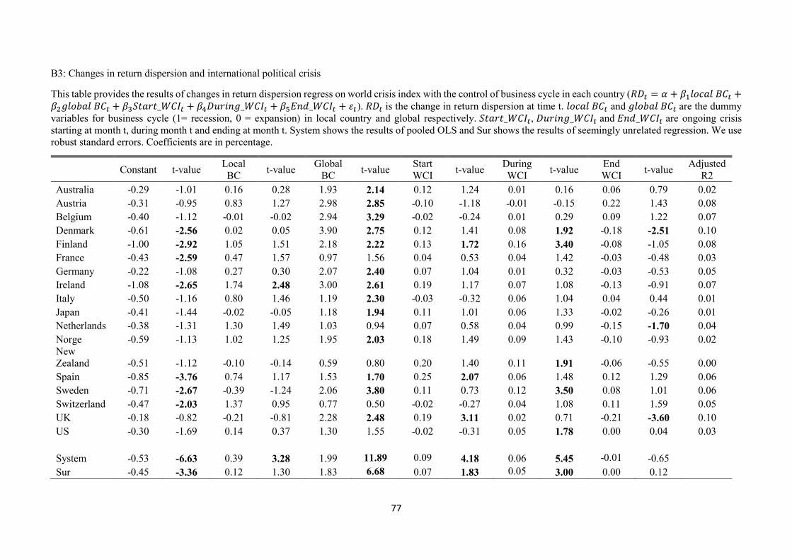
77
B3: Changes in return dispersion and international political crisis
This table provides the results of changes in return dispersion regress on world crisis index with the control of business cycle in each country (𝑅𝐷𝑡 = 𝛼 + 𝛽1𝑙𝑜𝑐𝑎𝑙 𝐵𝐶𝑡 +𝛽2𝑔𝑙𝑜𝑏𝑎𝑙 𝐵𝐶𝑡 + 𝛽3𝑆𝑡𝑎𝑟𝑡_𝑊𝐶𝐼𝑡 + 𝛽4𝐷𝑢𝑟𝑖𝑛𝑔_𝑊𝐶𝐼𝑡 + 𝛽5𝐸𝑛𝑑_𝑊𝐶𝐼𝑡 + 𝜀𝑡). 𝑅𝐷𝑡 is the change in return dispersion at time t. 𝑙𝑜𝑐𝑎𝑙 𝐵𝐶𝑡 and 𝑔𝑙𝑜𝑏𝑎𝑙 𝐵𝐶𝑡 are the dummy
variables for business cycle (1= recession, 0 = expansion) in local country and global respectively. 𝑆𝑡𝑎𝑟𝑡_𝑊𝐶𝐼𝑡, 𝐷𝑢𝑟𝑖𝑛𝑔_𝑊𝐶𝐼𝑡 and 𝐸𝑛𝑑_𝑊𝐶𝐼𝑡 are ongoing crisis
starting at month t, during month t and ending at month t. System shows the results of pooled OLS and Sur shows the results of seemingly unrelated regression. We use
robust standard errors. Coefficients are in percentage.
Constant t-value
Local
BC t-value
Global
BC t-value
Start
WCI t-value
During
WCI t-value
End
WCI t-value
Adjusted
R2
Australia -0.29 -1.01 0.16 0.28 1.93 2.14 0.12 1.24 0.01 0.16 0.06 0.79 0.02
Austria -0.31 -0.95 0.83 1.27 2.98 2.85 -0.10 -1.18 -0.01 -0.15 0.22 1.43 0.08
Belgium -0.40 -1.12 -0.01 -0.02 2.94 3.29 -0.02 -0.24 0.01 0.29 0.09 1.22 0.07
Denmark -0.61 -2.56 0.02 0.05 3.90 2.75 0.12 1.41 0.08 1.92 -0.18 -2.51 0.10
Finland -1.00 -2.92 1.05 1.51 2.18 2.22 0.13 1.72 0.16 3.40 -0.08 -1.05 0.08
France -0.43 -2.59 0.47 1.57 0.97 1.56 0.04 0.53 0.04 1.42 -0.03 -0.48 0.03
Germany -0.22 -1.08 0.27 0.30 2.07 2.40 0.07 1.04 0.01 0.32 -0.03 -0.53 0.05
Ireland -1.08 -2.65 1.74 2.48 3.00 2.61 0.19 1.17 0.07 1.08 -0.13 -0.91 0.07
Italy -0.50 -1.16 0.80 1.46 1.19 2.30 -0.03 -0.32 0.06 1.04 0.04 0.44 0.01
Japan -0.41 -1.44 -0.02 -0.05 1.18 1.94 0.11 1.01 0.06 1.33 -0.02 -0.26 0.01
Netherlands -0.38 -1.31 1.30 1.49 1.03 0.94 0.07 0.58 0.04 0.99 -0.15 -1.70 0.04
Norge -0.59 -1.13 1.02 1.25 1.95 2.03 0.18 1.49 0.09 1.43 -0.10 -0.93 0.02
New
Zealand -0.51 -1.12 -0.10 -0.14 0.59 0.80 0.20 1.40 0.11 1.91 -0.06 -0.55 0.00
Spain -0.85 -3.76 0.74 1.17 1.53 1.70 0.25 2.07 0.06 1.48 0.12 1.29 0.06
Sweden -0.71 -2.67 -0.39 -1.24 2.06 3.80 0.11 0.73 0.12 3.50 0.08 1.01 0.06
Switzerland -0.47 -2.03 1.37 0.95 0.77 0.50 -0.02 -0.27 0.04 1.08 0.11 1.59 0.05
UK -0.18 -0.82 -0.21 -0.81 2.28 2.48 0.19 3.11 0.02 0.71 -0.21 -3.60 0.10
US -0.30 -1.69 0.14 0.37 1.30 1.55 -0.02 -0.31 0.05 1.78 0.00 0.04 0.03
System -0.53 -6.63 0.39 3.28 1.99 11.89 0.09 4.18 0.06 5.45 -0.01 -0.65
Sur -0.45 -3.36 0.12 1.30 1.83 6.68 0.07 1.83 0.05 3.00 0.00 0.12

78
B4: Changes in return dispersion and word count uncertainty
This table reports the regression of changes in return dispersion on word count uncertainty around the world. We run the regression in the form of 𝑅𝐷𝑡 = 𝛼 +𝛽1𝑙𝑜𝑐𝑎𝑙_𝐵𝐶𝑡 + 𝛽2𝑔𝑙𝑜𝑏𝑎𝑙_𝐵𝐶𝑡 + 𝛽3𝑆𝑡𝑎𝑟𝑡 𝐶𝑟𝑖𝑠𝑖𝑠𝑡 + 𝛽4𝐷𝑢𝑟𝑖𝑛𝑔 𝐶𝑟𝑖𝑠𝑖𝑠𝑡 + 𝛽5𝐸𝑛𝑑 𝐶𝑟𝑖𝑠𝑖𝑠𝑡 + 𝛽6 𝑙𝑛(𝑤𝑜𝑟𝑑 𝑐𝑜𝑢𝑛𝑡 𝑢𝑛𝑐𝑒𝑟𝑡𝑎𝑖𝑛𝑡𝑦)𝑡 + 𝜀𝑡 where 𝑅𝐷𝑡 is the change in return
dispersion. Local BC and global BC are business cycle dummies, Start Crisis is crisis starting in month t, During Crisis is the ongoing crisis in month t and End Crisis
is the crisis ending in month t. Word count uncertainty is the number of Bloomberg reports in every month that contains the word “uncertainty” and take a log of it.
System shows the results of pooled OLS and Sur shows the results of seemingly unrelated regression. We use robust standard errors. Coefficients are in percentage.
constant t-value
local
BC t-value
global
BC t-value
start
Crisis t-value
during
Crisis t-value
end
Crisis t-value
Word count
uncertainty t-value
Adjusted
R2
Australia 0.95 0.79 0.02 0.03 2.26 2.41 0.10 1.03 0.00 0.03 0.04 0.48 -0.19 -1.07 0.02
Austria -2.33 -2.13 0.80 1.23 2.55 2.40 -0.06 -0.78 0.00 0.04 0.25 1.68 0.31 1.89 0.09
Belgium -2.26 -1.69 0.21 0.46 2.46 2.75 0.02 0.19 0.02 0.45 0.12 1.57 0.28 1.67 0.08
Denmark -3.11 -3.61 0.25 0.59 3.29 2.33 0.16 1.89 0.09 2.19 -0.14 -1.85 0.37 2.92 0.11
Finland -0.86 -0.64 1.03 1.40 2.22 2.16 0.12 1.60 0.16 3.27 -0.08 -1.00 -0.02 -0.12 0.08
France -1.38 -1.81 0.51 1.67 0.73 1.11 0.06 0.70 0.05 1.47 -0.01 -0.21 0.14 1.33 0.03
Germany -2.26 -3.18 0.62 0.68 1.49 1.73 0.10 1.51 0.02 0.60 -0.01 -0.09 0.31 2.88 0.07
Ireland -1.49 -0.95 1.71 2.38 2.92 2.42 0.20 1.15 0.07 1.08 -0.12 -0.84 0.06 0.27 0.06
Italy -2.37 -3.30 1.01 1.89 0.68 1.10 0.01 0.08 0.06 1.17 0.07 0.73 0.28 2.12 0.02
Japan -1.83 -1.94 0.02 0.06 0.83 1.31 0.13 1.24 0.06 1.43 0.00 0.05 0.21 1.66 0.02
Netherland
s -2.63 -2.47 1.25 1.48 0.56 0.47 0.11 0.90 0.05 1.25 -0.11 -1.35 0.34 2.05 0.05
Norge -1.90 -1.23 0.98 1.20 1.67 1.73 0.20 1.56 0.09 1.48 -0.08 -0.71 0.20 1.01 0.02
New
Zealand 4.15 2.59 0.07 0.10 1.64 2.15 0.11 0.81 0.09 1.63 -0.14 -1.22 -0.71 -3.18 0.05
Spain 0.75 0.86 0.78 1.22 1.86 2.06 0.22 1.84 0.05 1.29 0.09 0.99 -0.24 -1.87 0.07
Sweden -1.12 -1.52 -0.42 -1.33 1.98 3.41 0.12 0.79 0.12 3.54 0.09 1.07 0.06 0.55 0.06
Switzerland -2.60 -2.59 1.15 0.84 0.48 0.31 0.02 0.28 0.05 1.22 0.14 2.15 0.33 2.42 0.07
UK -1.80 -2.51 -0.02 -0.07 1.82 1.95 0.22 3.54 0.03 1.00 -0.18 -3.17 0.24 2.33 0.11
US -1.74 -2.77 0.20 0.55 0.92 1.09 0.01 0.20 0.06 1.95 0.03 0.43 0.22 2.40 0.05
System -1.36 -5.70 0.41 3.49 1.79 10.20 0.10 4.79 0.06 5.75 0.00 -0.01 0.13 3.71 Sur -1.31 -3.24 0.13 1.38 1.66 5.80 0.08 2.13 0.06 3.13 0.02 0.45 0.13 2.27
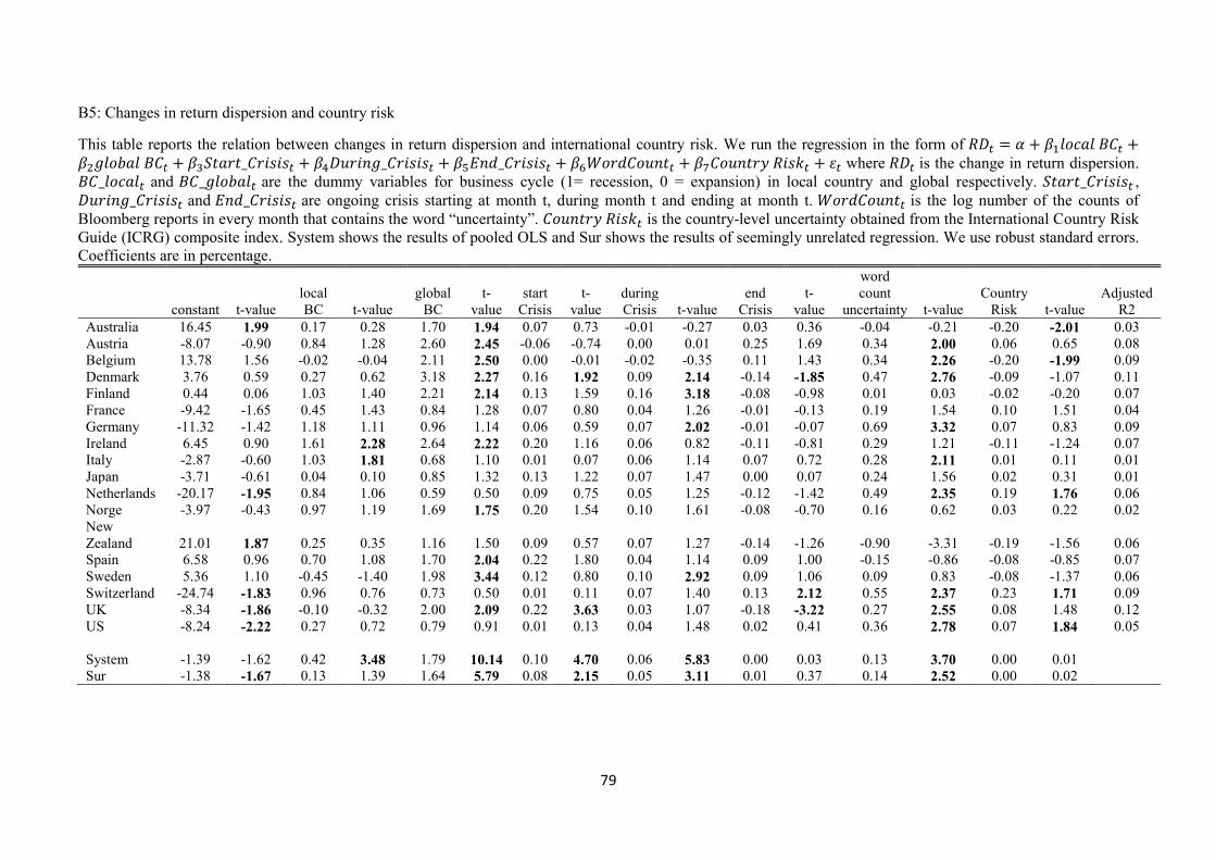
79
B5: Changes in return dispersion and country risk
This table reports the relation between changes in return dispersion and international country risk. We run the regression in the form of 𝑅𝐷𝑡 = 𝛼 + 𝛽1𝑙𝑜𝑐𝑎𝑙 𝐵𝐶𝑡 +𝛽2𝑔𝑙𝑜𝑏𝑎𝑙 𝐵𝐶𝑡 + 𝛽3𝑆𝑡𝑎𝑟𝑡_𝐶𝑟𝑖𝑠𝑖𝑠𝑡 + 𝛽4𝐷𝑢𝑟𝑖𝑛𝑔_𝐶𝑟𝑖𝑠𝑖𝑠𝑡 + 𝛽5𝐸𝑛𝑑_𝐶𝑟𝑖𝑠𝑖𝑠𝑡 + 𝛽6𝑊𝑜𝑟𝑑𝐶𝑜𝑢𝑛𝑡𝑡 + 𝛽7𝐶𝑜𝑢𝑛𝑡𝑟𝑦 𝑅𝑖𝑠𝑘𝑡 + 𝜀𝑡 where 𝑅𝐷𝑡 is the change in return dispersion.
𝐵𝐶_𝑙𝑜𝑐𝑎𝑙𝑡 and 𝐵𝐶_𝑔𝑙𝑜𝑏𝑎𝑙𝑡 are the dummy variables for business cycle (1= recession, 0 = expansion) in local country and global respectively. 𝑆𝑡𝑎𝑟𝑡_𝐶𝑟𝑖𝑠𝑖𝑠𝑡 ,
𝐷𝑢𝑟𝑖𝑛𝑔_𝐶𝑟𝑖𝑠𝑖𝑠𝑡 and 𝐸𝑛𝑑_𝐶𝑟𝑖𝑠𝑖𝑠𝑡 are ongoing crisis starting at month t, during month t and ending at month t. 𝑊𝑜𝑟𝑑𝐶𝑜𝑢𝑛𝑡𝑡 is the log number of the counts of
Bloomberg reports in every month that contains the word “uncertainty”. 𝐶𝑜𝑢𝑛𝑡𝑟𝑦 𝑅𝑖𝑠𝑘𝑡 is the country-level uncertainty obtained from the International Country Risk
Guide (ICRG) composite index. System shows the results of pooled OLS and Sur shows the results of seemingly unrelated regression. We use robust standard errors.
Coefficients are in percentage.
constant t-value
local
BC t-value
global
BC
t-
value
start
Crisis
t-
value
during
Crisis t-value
end
Crisis
t-
value
word
count
uncertainty t-value
Country
Risk t-value
Adjusted
R2
Australia 16.45 1.99 0.17 0.28 1.70 1.94 0.07 0.73 -0.01 -0.27 0.03 0.36 -0.04 -0.21 -0.20 -2.01 0.03
Austria -8.07 -0.90 0.84 1.28 2.60 2.45 -0.06 -0.74 0.00 0.01 0.25 1.69 0.34 2.00 0.06 0.65 0.08
Belgium 13.78 1.56 -0.02 -0.04 2.11 2.50 0.00 -0.01 -0.02 -0.35 0.11 1.43 0.34 2.26 -0.20 -1.99 0.09
Denmark 3.76 0.59 0.27 0.62 3.18 2.27 0.16 1.92 0.09 2.14 -0.14 -1.85 0.47 2.76 -0.09 -1.07 0.11
Finland 0.44 0.06 1.03 1.40 2.21 2.14 0.13 1.59 0.16 3.18 -0.08 -0.98 0.01 0.03 -0.02 -0.20 0.07
France -9.42 -1.65 0.45 1.43 0.84 1.28 0.07 0.80 0.04 1.26 -0.01 -0.13 0.19 1.54 0.10 1.51 0.04
Germany -11.32 -1.42 1.18 1.11 0.96 1.14 0.06 0.59 0.07 2.02 -0.01 -0.07 0.69 3.32 0.07 0.83 0.09
Ireland 6.45 0.90 1.61 2.28 2.64 2.22 0.20 1.16 0.06 0.82 -0.11 -0.81 0.29 1.21 -0.11 -1.24 0.07
Italy -2.87 -0.60 1.03 1.81 0.68 1.10 0.01 0.07 0.06 1.14 0.07 0.72 0.28 2.11 0.01 0.11 0.01
Japan -3.71 -0.61 0.04 0.10 0.85 1.32 0.13 1.22 0.07 1.47 0.00 0.07 0.24 1.56 0.02 0.31 0.01
Netherlands -20.17 -1.95 0.84 1.06 0.59 0.50 0.09 0.75 0.05 1.25 -0.12 -1.42 0.49 2.35 0.19 1.76 0.06
Norge -3.97 -0.43 0.97 1.19 1.69 1.75 0.20 1.54 0.10 1.61 -0.08 -0.70 0.16 0.62 0.03 0.22 0.02
New
Zealand 21.01 1.87 0.25 0.35 1.16 1.50 0.09 0.57 0.07 1.27 -0.14 -1.26 -0.90 -3.31 -0.19 -1.56 0.06
Spain 6.58 0.96 0.70 1.08 1.70 2.04 0.22 1.80 0.04 1.14 0.09 1.00 -0.15 -0.86 -0.08 -0.85 0.07
Sweden 5.36 1.10 -0.45 -1.40 1.98 3.44 0.12 0.80 0.10 2.92 0.09 1.06 0.09 0.83 -0.08 -1.37 0.06
Switzerland -24.74 -1.83 0.96 0.76 0.73 0.50 0.01 0.11 0.07 1.40 0.13 2.12 0.55 2.37 0.23 1.71 0.09
UK -8.34 -1.86 -0.10 -0.32 2.00 2.09 0.22 3.63 0.03 1.07 -0.18 -3.22 0.27 2.55 0.08 1.48 0.12
US -8.24 -2.22 0.27 0.72 0.79 0.91 0.01 0.13 0.04 1.48 0.02 0.41 0.36 2.78 0.07 1.84 0.05
System -1.39 -1.62 0.42 3.48 1.79 10.14 0.10 4.70 0.06 5.83 0.00 0.03 0.13 3.70 0.00 0.01 Sur -1.38 -1.67 0.13 1.39 1.64 5.79 0.08 2.15 0.05 3.11 0.01 0.37 0.14 2.52 0.00 0.02

80
B6: Changes in return dispersion and economic policy uncertainty
This table reports the results of changes in return dispersion regress on both local and global economic policy uncertainty. Regressions are in the form of: 𝑅𝐷𝑡 = 𝛼 +
𝛽1𝐿𝑜𝑐𝑎𝑙 𝐵𝐶𝑡 + 𝛽2𝐺𝑙𝑜𝑏𝑎𝑙 𝐵𝐶𝑡 + 𝛽3𝑆𝑡𝑎𝑟𝑡 𝐶𝑟𝑖𝑠𝑖𝑠𝑡 + 𝛽4𝐷𝑢𝑟𝑖𝑛𝑔 𝐶𝑟𝑖𝑠𝑖𝑠𝑡 + 𝛽5𝐸𝑛𝑑 𝐶𝑟𝑖𝑠𝑖𝑠𝑡 + 𝛽6𝑊𝑜𝑟𝑑𝐶𝑜𝑢𝑛𝑡𝑡 + 𝛽7𝐶𝑜𝑢𝑛𝑡𝑟𝑦𝑅𝑖𝑠𝑘𝑡+ 𝛽8 ln(𝐸𝑃𝑈𝑙𝑜𝑐𝑎𝑙)𝑡 +𝛽9 ln(𝐸𝑃𝑈𝑔𝑙𝑜𝑏𝑎𝑙)
𝑡+ 𝜀𝑡
where 𝑅𝐷𝑡 is the change in return dispersion. We include two economic policy index, one is the country specific index (𝐸𝑃𝑈_𝑙𝑜𝑐𝑎𝑙) and the other is the global
index (𝐸𝑃𝑈_𝑔𝑙𝑜𝑏𝑎𝑙). System shows the results of pooled OLS and Sur shows the results of seemingly unrelated regression. We use robust standard errors. Coefficients
are in percentage.
Country Coefficient Constant
Local
BC
Global
BC
Start
Crisis
During
Crisis
end
Crisis
Word Count
Uncertainty
Country
Risk
ln(Local
EPU)
ln(Global
EPU) N
Adjusted
R2
Australia Coeff. (%) -1.16 1.04 0.95 0.17 -0.08 0.31 0.56 0.00 2.93 -3.60 144 0.13
t-Stat -0.08 0.52 1.04 1.09 -1.00 1.94 1.09 0.02 3.41 -2.44 France Coeff. (%) -11.34 0.29 0.26 -0.05 0.10 -0.10 -0.24 0.03 -0.26 2.64 156 0.09
t-Stat -0.93 0.38 0.33 -0.25 1.24 -1.18 -0.50 0.25 -0.54 2.52 Germany Coeff. (%) -15.04 1.40 0.54 0.03 0.09 -0.02 0.06 0.06 0.43 1.74 156 0.07
t-Stat -1.04 0.63 0.54 0.21 1.58 -0.15 0.16 0.41 0.66 1.41 Ireland Coeff. (%) -9.76 1.37 2.41 0.26 0.04 -0.15 -0.10 -0.01 0.92 1.60 156 0.05
t-Stat -0.55 1.52 1.91 0.63 0.37 -0.44 -0.15 -0.11 0.94 0.85 Italy Coeff. (%) -6.09 1.14 0.70 -0.04 0.10 0.07 -0.50 -0.07 2.06 1.21 156 0.02
t-Stat -0.63 1.45 1.44 -0.28 0.95 0.33 -1.17 -0.69 2.73 1.30 Japan Coeff. (%) -5.94 0.19 0.80 0.16 0.13 0.00 0.43 0.04 0.99 -1.26 156 0.00
t-Stat -0.54 0.30 1.05 1.18 1.77 -0.04 0.69 0.45 1.05 -1.01 Netherland Coeff. (%) 10.02 1.71 1.36 -0.18 -0.06 -0.23 -0.99 -0.09 -0.67 1.72 82 0.06
t-Stat 0.61 0.71 1.11 -1.02 -0.49 -1.57 -1.05 -0.50 -0.55 0.71 Spain Coeff. (%) 0.14 1.29 0.95 0.04 0.11 0.13 -0.74 -0.05 -0.28 2.08 108 0.08
t-Stat 0.01 1.48 0.90 0.13 1.11 0.62 -0.83 -0.27 -0.39 1.28 Sweden Coeff. (%) -2.49 -0.38 1.41 -0.02 0.07 0.13 0.88 -0.16 1.94 0.18 156 0.11
t-Stat -0.23 -0.84 2.16 -0.15 1.41 0.94 1.44 -1.64 1.39 0.16 UK Coeff. (%) -12.50 -0.04 1.19 0.16 0.04 -0.24 0.21 0.01 -1.50 3.80 156 0.13
t-Stat -1.58 -0.08 1.23 1.25 0.76 -2.32 0.49 0.13 -2.03 2.91 US Coeff. (%) -14.13 0.18 0.45 -0.03 0.08 0.00 -0.10 0.09 1.60 0.18 156 0.04
t-Stat -1.91 0.31 0.51 -0.29 1.33 -0.01 -0.23 1.59 0.96 0.13
System Coeff. (%) -8.37 0.43 1.20 0.06 0.09 0.00 -0.14 0.02 0.47 1.25
t-Stat -3.42 1.90 4.48 1.13 4.18 0.08 -0.74 0.76 2.10 3.36 Sur Coeff. (%) -6.24 0.18 1.25 0.06 0.09 0.05 -0.05 0.01 0.20 1.08 t-Stat -2.43 1.06 3.70 0.84 2.96 0.89 -0.18 0.33 1.19 2.44

81
B7. Changes in return dispersion and cross section of returns
This table reports the four factor alphas of portfolios sorted by their sensitivity to changes in return dispersion. The four factors are market, size, value and momentum
factors. We report the monthly value-weighted portfolio returns in panel A and equal-weighted portfolio returns in panel B. The coefficients are in percentage.
Panel A: value weighted portfolio four-factor alphas
Low Group 2 Group 3 Group 4 High High - Low
Mean t-value Mean t-value Mean t-value Mean t-value Mean t-value Mean t-value
Australia -3.77 -10.55 -0.85 -3.80 0.07 0.42 1.04 5.18 1.94 5.88 5.70 11.74
Belgium -2.56 -5.22 -0.33 -0.97 0.34 1.35 0.20 0.72 2.05 5.31 4.61 7.38
France -2.65 -7.57 -0.94 -3.94 -0.14 -0.68 0.57 2.57 2.24 7.38 4.90 10.56
Germany -2.88 -6.31 -0.73 -2.82 -0.10 -0.39 0.59 2.25 1.87 4.75 4.76 7.89
Italy -2.88 -7.19 -1.01 -3.09 -0.65 -2.08 0.11 0.33 1.80 4.77 4.67 8.50
Japan -2.89 -10.08 -1.54 -7.69 -0.87 -4.90 0.12 0.65 1.86 7.33 4.75 12.41
Netherland -3.35 -8.16 -0.80 -2.43 0.03 0.11 0.53 1.74 2.58 6.72 5.93 10.55
Norway -4.05 -7.44 -1.02 -2.98 -0.15 -0.40 0.52 1.46 2.49 5.05 6.54 8.91
Spain -3.30 -6.44 -0.76 -2.52 -0.17 -0.59 0.58 1.78 2.24 6.20 5.54 8.84
Sweden -3.25 -7.18 -0.37 -1.03 0.19 0.55 1.52 4.52 3.46 8.03 6.71 10.74
Switzerland -2.68 -6.97 -0.33 -1.28 0.08 0.33 0.44 1.35 2.77 7.24 5.45 10.05
UK -3.22 -9.27 -0.63 -2.80 0.14 0.74 0.66 3.22 2.21 8.89 5.43 12.71
US -1.94 -11.81 -0.58 -7.06 0.06 0.98 0.52 8.41 1.67 9.31 3.61 14.83
average -3.03 -0.76 -0.09 0.57 2.25 5.28 min -4.05 -1.54 -0.87 0.11 1.67 3.61 max -1.94 -0.33 0.34 1.52 3.46 6.71 median -2.89 -0.76 0.03 0.53 2.21 5.43
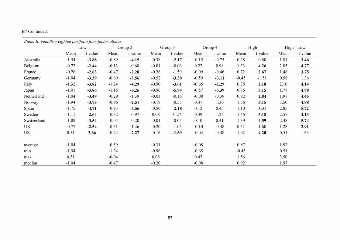
82
B7 Continued.
Panel B: equally weighted portfolio four-factor alphas
Low Group 2 Group 3 Group 4 High High - Low
Mean t-value Mean t-value Mean t-value Mean t-value Mean t-value Mean t-value
Australia -1.54 -3.88 -0.89 -4.15 -0.38 -2.17 -0.15 -0.75 0.28 0.80 1.81 3.46
Belgium -0.72 -2.44 -0.13 -0.60 -0.01 -0.06 0.22 0.98 1.33 4.26 2.05 4.77
France -0.76 -2.63 -0.47 -2.28 -0.26 -1.59 -0.09 -0.46 0.72 2.67 1.48 3.75
Germany -1.04 -3.39 -0.69 -3.56 -0.52 -3.30 -0.59 -3.11 -0.45 -1.51 0.58 1.36
Italy -1.32 -3.82 -1.24 -4.29 -0.90 -3.61 -0.65 -2.29 0.78 2.10 2.10 4.14
Japan -1.01 -3.86 -1.15 -6.26 -0.96 -5.94 -0.57 -3.39 0.76 3.15 1.77 4.98
Netherland -1.04 -3.48 -0.29 -1.39 -0.03 -0.16 -0.08 -0.39 0.92 2.84 1.97 4.45
Norway -1.94 -3.75 -0.96 -2.51 -0.19 -0.55 0.47 1.36 1.56 3.15 3.50 4.88
Spain -1.75 -4.71 -0.93 -3.56 -0.50 -2.18 0.12 0.45 1.10 3.31 2.85 5.72
Sweden -1.11 -2.64 -0.32 -0.97 0.08 0.27 0.39 1.23 1.46 3.18 2.57 4.13
Switzerland -1.09 -3.54 -0.04 -0.20 -0.01 -0.05 0.10 0.41 1.39 4.59 2.48 5.74
UK -0.77 -2.54 -0.31 -1.46 -0.20 -1.05 -0.10 -0.48 0.51 1.60 1.28 2.91
US 0.51 2.66 -0.24 -2.27 -0.16 -1.69 -0.04 -0.48 1.02 4.20 0.51 1.63
average -1.04 -0.59 -0.31 -0.08 0.87 1.92 min -1.94 -1.24 -0.96 -0.65 -0.45 0.51 max 0.51 -0.04 0.08 0.47 1.56 3.50 median -1.04 -0.47 -0.20 -0.08 0.92 1.97
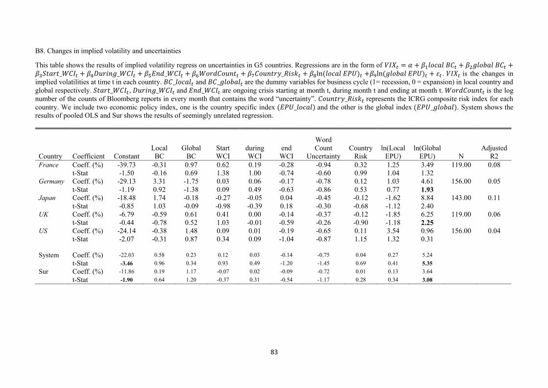
83
B8. Changes in implied volatility and uncertainties
This table shows the results of implied volatility regress on uncertainties in G5 countries. Regressions are in the form of 𝑉𝐼𝑋𝑡 = 𝛼 + 𝛽1𝑙𝑜𝑐𝑎𝑙 𝐵𝐶𝑡 + 𝛽2𝑔𝑙𝑜𝑏𝑎𝑙 𝐵𝐶𝑡 +𝛽3𝑆𝑡𝑎𝑟𝑡_𝑊𝐶𝐼𝑡 + 𝛽4𝐷𝑢𝑟𝑖𝑛𝑔_𝑊𝐶𝐼𝑡 + 𝛽5𝐸𝑛𝑑_𝑊𝐶𝐼𝑡 + 𝛽6𝑊𝑜𝑟𝑑𝐶𝑜𝑢𝑛𝑡𝑡 + 𝛽7𝐶𝑜𝑢𝑛𝑡𝑟𝑦_𝑅𝑖𝑠𝑘𝑡 + 𝛽8ln (𝑙𝑜𝑐𝑎𝑙 𝐸𝑃𝑈)𝑡 +𝛽9ln (𝑔𝑙𝑜𝑏𝑎𝑙 𝐸𝑃𝑈)𝑡 + 𝜀𝑡 . 𝑉𝐼𝑋𝑡 is the changes in
implied volatilities at time t in each country. 𝐵𝐶_𝑙𝑜𝑐𝑎𝑙𝑡 and 𝐵𝐶_𝑔𝑙𝑜𝑏𝑎𝑙𝑡 are the dummy variables for business cycle (1= recession, 0 = expansion) in local country and
global respectively. 𝑆𝑡𝑎𝑟𝑡_𝑊𝐶𝐼𝑡, 𝐷𝑢𝑟𝑖𝑛𝑔_𝑊𝐶𝐼𝑡 and 𝐸𝑛𝑑_𝑊𝐶𝐼𝑡 are ongoing crisis starting at month t, during month t and ending at month t. 𝑊𝑜𝑟𝑑𝐶𝑜𝑢𝑛𝑡𝑡 is the log
number of the counts of Bloomberg reports in every month that contains the word “uncertainty”. 𝐶𝑜𝑢𝑛𝑡𝑟𝑦_𝑅𝑖𝑠𝑘𝑡 represents the ICRG composite risk index for each
country. We include two economic policy index, one is the country specific index (𝐸𝑃𝑈_𝑙𝑜𝑐𝑎𝑙) and the other is the global index (𝐸𝑃𝑈_𝑔𝑙𝑜𝑏𝑎𝑙). System shows the
results of pooled OLS and Sur shows the results of seemingly unrelated regression.
Country Coefficient Constant
Local
BC
Global
BC
Start
WCI
during
WCI
end
WCI
Word
Count
Uncertainty
Country
Risk
ln(Local
EPU)
ln(Global
EPU) N
Adjusted
R2
France Coeff. (%) -39.73 -0.31 0.97 0.62 0.19 -0.28 -0.94 0.32 1.25 3.49 119.00 0.08
t-Stat -1.50 -0.16 0.69 1.38 1.00 -0.74 -0.60 0.99 1.04 1.32 Germany Coeff. (%) -29.13 3.31 -1.75 0.03 0.06 -0.17 -0.78 0.12 1.03 4.61 156.00 0.05
t-Stat -1.19 0.92 -1.38 0.09 0.49 -0.63 -0.86 0.53 0.77 1.93 Japan Coeff. (%) -18.48 1.74 -0.18 -0.27 -0.05 0.04 -0.45 -0.12 -1.62 8.84 143.00 0.11
t-Stat -0.85 1.03 -0.09 -0.98 -0.39 0.18 -0.30 -0.68 -1.12 2.40 UK Coeff. (%) -6.79 -0.59 0.61 0.41 0.00 -0.14 -0.37 -0.12 -1.85 6.25 119.00 0.06
t-Stat -0.44 -0.78 0.52 1.03 -0.01 -0.59 -0.26 -0.90 -1.18 2.25 US Coeff. (%) -24.14 -0.38 1.48 0.09 0.01 -0.19 -0.65 0.11 3.54 0.96 156.00 0.04
t-Stat -2.07 -0.31 0.87 0.34 0.09 -1.04 -0.87 1.15 1.32 0.31
System Coeff. (%) -22.03 0.58 0.23 0.12 0.03 -0.14 -0.75 0.04 0.27 5.24
t-Stat -3.46 0.96 0.34 0.93 0.49 -1.20 -1.45 0.69 0.41 5.35 Sur Coeff. (%) -11.86 0.19 1.17 -0.07 0.02 -0.09 -0.72 0.01 0.13 3.64 t-Stat -1.90 0.64 1.20 -0.37 0.31 -0.54 -1.17 0.28 0.34 3.08
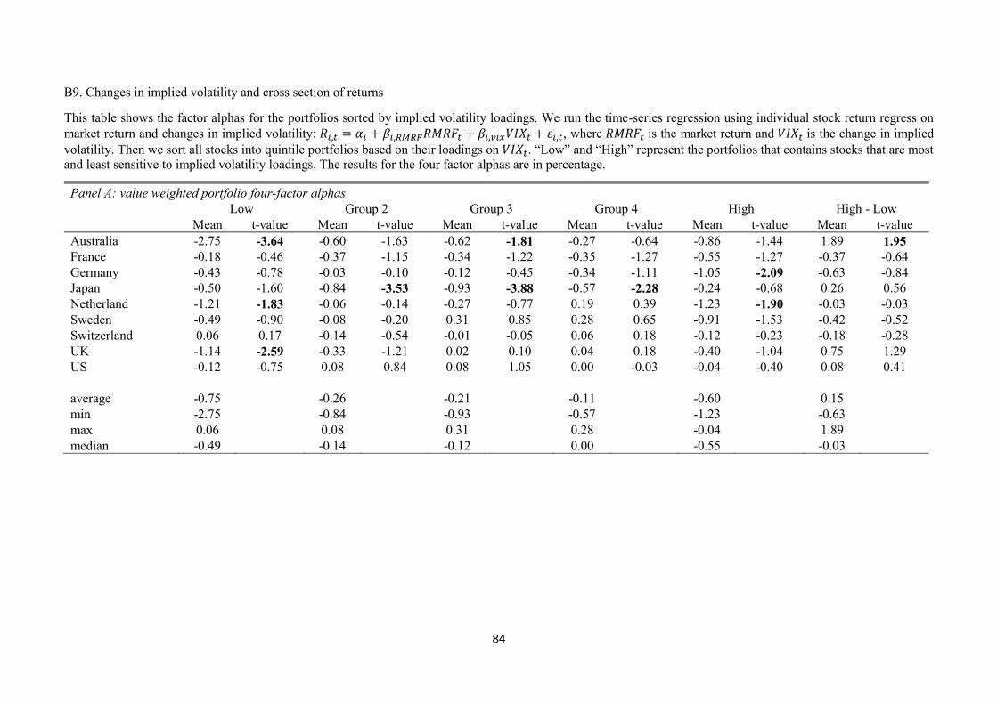
84
B9. Changes in implied volatility and cross section of returns
This table shows the factor alphas for the portfolios sorted by implied volatility loadings. We run the time-series regression using individual stock return regress on
market return and changes in implied volatility: 𝑅𝑖,𝑡 = 𝛼𝑖 + 𝛽𝑖,𝑅𝑀𝑅𝐹𝑅𝑀𝑅𝐹𝑡 + 𝛽𝑖,𝑣𝑖𝑥𝑉𝐼𝑋𝑡 + 𝜀𝑖,𝑡, where 𝑅𝑀𝑅𝐹𝑡 is the market return and 𝑉𝐼𝑋𝑡 is the change in implied
volatility. Then we sort all stocks into quintile portfolios based on their loadings on 𝑉𝐼𝑋𝑡. “Low” and “High” represent the portfolios that contains stocks that are most
and least sensitive to implied volatility loadings. The results for the four factor alphas are in percentage.
Panel A: value weighted portfolio four-factor alphas
Low Group 2 Group 3 Group 4 High High - Low
Mean t-value Mean t-value Mean t-value Mean t-value Mean t-value Mean t-value
Australia -2.75 -3.64 -0.60 -1.63 -0.62 -1.81 -0.27 -0.64 -0.86 -1.44 1.89 1.95
France -0.18 -0.46 -0.37 -1.15 -0.34 -1.22 -0.35 -1.27 -0.55 -1.27 -0.37 -0.64
Germany -0.43 -0.78 -0.03 -0.10 -0.12 -0.45 -0.34 -1.11 -1.05 -2.09 -0.63 -0.84
Japan -0.50 -1.60 -0.84 -3.53 -0.93 -3.88 -0.57 -2.28 -0.24 -0.68 0.26 0.56
Netherland -1.21 -1.83 -0.06 -0.14 -0.27 -0.77 0.19 0.39 -1.23 -1.90 -0.03 -0.03
Sweden -0.49 -0.90 -0.08 -0.20 0.31 0.85 0.28 0.65 -0.91 -1.53 -0.42 -0.52
Switzerland 0.06 0.17 -0.14 -0.54 -0.01 -0.05 0.06 0.18 -0.12 -0.23 -0.18 -0.28
UK -1.14 -2.59 -0.33 -1.21 0.02 0.10 0.04 0.18 -0.40 -1.04 0.75 1.29
US -0.12 -0.75 0.08 0.84 0.08 1.05 0.00 -0.03 -0.04 -0.40 0.08 0.41
average -0.75 -0.26 -0.21 -0.11 -0.60 0.15 min -2.75 -0.84 -0.93 -0.57 -1.23 -0.63 max 0.06 0.08 0.31 0.28 -0.04 1.89 median -0.49 -0.14 -0.12 0.00 -0.55 -0.03

85
Panel B: equally weighted portfolio four-factor alphas
Low Group 2 Group 3 Group 4 High High - Low
Mean t-value Mean t-value Mean t-value Mean t-value Mean t-value Mean t-value
Australia -2.39 -4.00 -2.40 -5.55 -1.75 -4.86 -1.73 -4.37 -0.91 -1.40 1.48 1.67
France -0.46 -1.14 -0.69 -2.72 -0.59 -2.55 -0.63 -2.64 0.08 0.19 0.53 0.95
Germany -1.30 -3.39 -0.81 -3.70 -0.65 -3.79 -0.66 -3.03 -0.59 -1.63 0.71 1.35
Japan -0.27 -0.91 -1.00 -4.77 -0.98 -4.99 -0.80 -3.64 0.21 0.64 0.47 1.09
Netherland -1.03 -2.40 -0.60 -1.80 -0.25 -0.96 -0.68 -2.29 -1.01 -1.95 0.02 0.03
Sweden -1.50 -3.70 -0.98 -3.23 -0.32 -1.05 -0.60 -1.85 -0.45 -0.99 1.05 1.72
Switzerland -0.42 -1.33 -0.14 -0.69 -0.09 -0.53 0.09 0.44 0.07 0.21 -0.28 1.04
UK -1.21 -3.96 -0.75 -3.64 -0.57 -3.10 -0.51 -2.68 -2.68 -1.64 0.71 1.65
US 0.14 0.88 -0.06 -0.64 -0.05 -0.71 -0.03 -0.34 0.24 2.27 0.10 0.53
average -0.94 -0.83 -0.58 -0.62 -0.56 0.53 min -2.39 -2.40 -1.75 -1.73 -2.68 -0.28 max 0.14 -0.06 -0.05 0.09 0.24 1.48 median -1.03 -0.75 -0.57 -0.63 -0.45 0.53

86
Appendix C This appendix contains the robustness results of return dispersion made by market index constituents. For Australia, Finland, France, Germany, Japan, Switzerland and
the US, we construct return dispersion series using all constituents of their major market indices.
Table C1. Local business cycle
This table shows the results of the regressions estimated in Table 2 using return dispersion made by market index constituents as the dependent variable. Local BC is a
dummy variable that equals one if the country is in recession and zero otherwise. System shows the results of pooled OLS and Sur shows the results of seemingly
unrelated regression. We use robust standard errors. Coefficients are in percentage.
constant t-value local BC t-value Adjusted R2
Australia 10.97 53.96 2.33 1.77 0.03
Finland 8.78 25.21 1.80 1.81 0.01
France 6.25 32.34 1.89 4.94 0.10
Germany 6.45 34.54 2.16 1.41 0.03
Japan 7.58 42.91 1.60 3.80 0.06
Switzerland 6.27 34.92 2.30 4.12 0.09
US 8.30 49.30 3.78 7.01 0.23
System 1.72 7.44
Sur 0.86 5.60
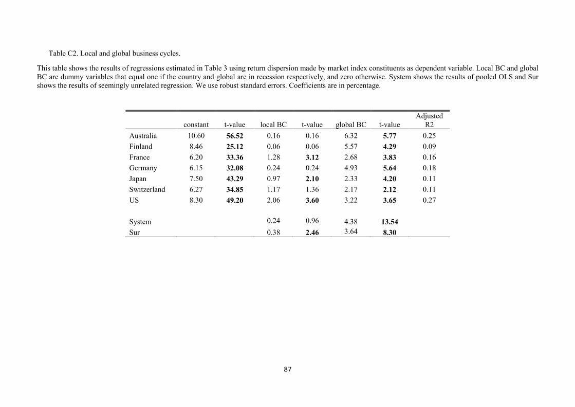
87
Table C2. Local and global business cycles.
This table shows the results of regressions estimated in Table 3 using return dispersion made by market index constituents as dependent variable. Local BC and global
BC are dummy variables that equal one if the country and global are in recession respectively, and zero otherwise. System shows the results of pooled OLS and Sur
shows the results of seemingly unrelated regression. We use robust standard errors. Coefficients are in percentage.
constant t-value local BC t-value global BC t-value
Adjusted
R2
Australia 10.60 56.52 0.16 0.16 6.32 5.77 0.25
Finland 8.46 25.12 0.06 0.06 5.57 4.29 0.09
France 6.20 33.36 1.28 3.12 2.68 3.83 0.16
Germany 6.15 32.08 0.24 0.24 4.93 5.64 0.18
Japan 7.50 43.29 0.97 2.10 2.33 4.20 0.11
Switzerland 6.27 34.85 1.17 1.36 2.17 2.12 0.11
US 8.30 49.20 2.06 3.60 3.22 3.65 0.27
System 0.24 0.96 4.38 13.54
Sur 0.38 2.46 3.64 8.30
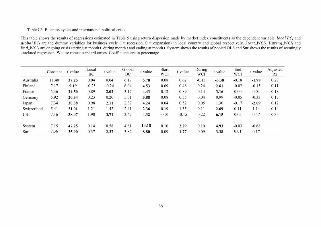
88
Table C3. Business cycles and international political crisis
This table shows the results of regressions estimated in Table 5 using return dispersion made by market index constituents as the dependent variable. 𝑙𝑜𝑐𝑎𝑙 𝐵𝐶𝑡 and
𝑔𝑙𝑜𝑏𝑎𝑙 𝐵𝐶𝑡 are the dummy variables for business cycle (1= recession, 0 = expansion) in local country and global respectively. 𝑆𝑡𝑎𝑟𝑡_𝑊𝐶𝐼𝑡 , 𝐷𝑢𝑟𝑖𝑛𝑔_𝑊𝐶𝐼𝑡 and
𝐸𝑛𝑑_𝑊𝐶𝐼𝑡 are ongoing crisis starting at month t, during month t and ending at month t. System shows the results of pooled OLS and Sur shows the results of seemingly
unrelated regression. We use robust standard errors. Coefficients are in percentage.
Constant t-value
Local
BC t-value
Global
BC t-value
Start
WCI t-value
During
WCI t-value
End
WCI t-value
Adjusted
R2
Australia 11.40 37.25 0.04 0.04 6.17 5.78 0.08 0.62 -0.13 -3.38 -0.18 -1.98 0.27
Finland 7.17 9.19 -0.25 -0.24 6.04 4.53 0.09 0.48 0.24 2.61 -0.02 -0.15 0.11
France 5.46 24.50 0.89 2.02 3.17 4.43 0.12 0.89 0.14 3.16 0.00 0.04 0.18
Germany 5.92 20.54 0.23 0.20 5.01 5.88 0.08 0.55 0.04 0.99 -0.05 -0.33 0.17
Japan 7.34 30.38 0.98 2.11 2.37 4.24 0.04 0.52 0.05 1.30 -0.17 -2.09 0.12
Switzerland 5.41 21.01 1.21 1.42 2.41 2.36 0.19 1.55 0.11 2.69 0.11 1.14 0.14
US 7.16 38.07 1.90 3.71 3.67 4.32 -0.01 -0.15 0.22 6.15 0.05 0.47 0.35
System 7.15 47.25 0.14 0.58 4.61 14.18 0.10 2.29 0.10 4.93 -0.03 -0.68
Sur 7.36 35.90 0.37 2.37 3.82 8.80 0.09 1.77 0.09 3.38 0.01 0.17

89
Table C4. Business cycle, international political crisis and word count uncertainty.
This table reports the results of regressions estimated in Table 6 using return dispersion made by market index constituents as the dependent variable. Local BC and
global BC are business cycle dummies, Start Crisis is crisis starting in month t, During Crisis is the ongoing crisis in month t and End Crisis is the crisis ending in month
t. Word count uncertainty is the number of Bloomberg reports in every month that contains the word “uncertainty” and take a log of it. System shows the results of
pooled OLS and Sur shows the results of seemingly unrelated regression. We use robust standard errors. Coefficients are in percentage.
constant
t-
value
local
BC
t-
value
global
BC t-value
start
Crisis
t-
value
during
Crisis
t-
value
end
Crisis
t-
value
Word Count
Uncertainty
t-
value
Adjusted
R2
Australia 9.45 7.70 0.24 0.24 5.73 5.33 0.10 0.83 -0.12 -3.14 -0.17 -1.79 0.28 1.61 0.28
Finland 5.02 1.24 0.15 0.12 5.49 3.70 0.11 0.55 0.25 2.48 0.00 -0.01 0.32 0.63 0.11
France 0.74 0.75 0.93 2.33 2.25 3.06 0.18 1.38 0.16 3.66 0.05 0.38 0.70 5.06 0.26
Germany -1.97 -1.65 1.93 1.77 2.91 3.83 0.14 1.10 0.07 1.89 -0.02 -0.16 1.17 6.75 0.31
Japan 3.37 3.60 1.27 2.84 1.46 2.47 0.08 0.95 0.07 1.73 -0.14 -1.83 0.58 4.51 0.18
Switzerland 1.28 1.21 0.96 1.28 1.85 1.87 0.23 2.10 0.13 3.13 0.15 1.58 0.61 4.01 0.19
US 2.15 2.74 2.31 4.98 2.35 2.73 0.04 0.64 0.24 7.37 0.09 1.01 0.74 6.34 0.42
System 3.74 8.00 0.33 1.35 3.79 11.24 0.15 3.30 0.11 5.52 0.01 0.35 0.51 7.69 Sur 5.11 8.62 0.40 2.60 3.47 7.95 0.13 2.45 0.10 3.87 0.05 0.89 0.33 3.92

90
Table C5. Business cycles, international political crisis, word count uncertainty and country risk.
This table reports the results of regressions estimated in Table 7 using return dispersion made by market index constituents as the dependent variable. Local BC and
global BC are business cycle dummies, Start Crisis is crisis starting in month t, During Crisis is the ongoing crisis in month t and End Crisis is the crisis ending in month
t. Word count uncertainty is the number of Bloomberg reports in every month that contains the word “uncertainty” and take a log of it. Country Risk is the International
Country Risk Guide (ICRG) composite index. System shows the results of pooled OLS and Sur shows the results of seemingly unrelated regression. We use robust
standard errors. Coefficients are in percentage.
constant
t-
value
local
BC
t-
value
global
BC
t-
value
start
Crisis
t-
value
during
Crisis
t-
value
end
Crisis
t-
value
word
count
uncertainty
t-
value
Country
Risk
t-
value
Adjusted
R2
Australia 76.08 9.01 0.52 0.67 3.68 4.13 -0.03 -0.36 -0.18 -4.66 -0.17 -1.95 0.69 4.34 -0.85 -8.01 0.43
Finland -7.78 -0.84 0.03 0.02 5.68 3.74 0.11 0.53 0.27 2.92 -0.01 -0.04 -0.04 -0.06 0.18 1.30 0.11
France -23.81 -3.16 0.70 1.69 2.55 3.28 0.19 1.58 0.13 3.10 0.05 0.47 0.91 5.48 0.29 3.46 0.30
Germany -14.68 -1.77 3.06 2.71 1.97 2.73 0.14 1.07 0.17 4.05 -0.03 -0.22 1.88 7.88 0.09 0.90 0.37
Japan 14.56 2.56 1.23 2.74 1.29 2.20 0.06 0.63 0.04 1.03 -0.15 -1.97 0.44 3.02 -0.12 -1.97 0.19
Switzerland -17.78 -1.85 0.77 1.14 2.13 2.27 0.23 2.17 0.14 3.51 0.14 1.59 0.76 4.22 0.20 2.05 0.20
US -9.78 -2.09 2.44 5.42 2.08 2.34 0.04 0.63 0.20 6.33 0.09 0.93 1.00 6.74 0.13 2.57 0.44
System 10.95 6.20 0.25 1.02 3.83 11.33 0.15 3.20 0.11 5.16 0.01 0.34 0.44 6.39 -0.08 -4.12 Sur 8.89 7.23 0.37 2.21 3.47 7.89 0.14 2.64 0.11 4.17 0.04 0.75 0.32 3.94 -0.04 -3.63
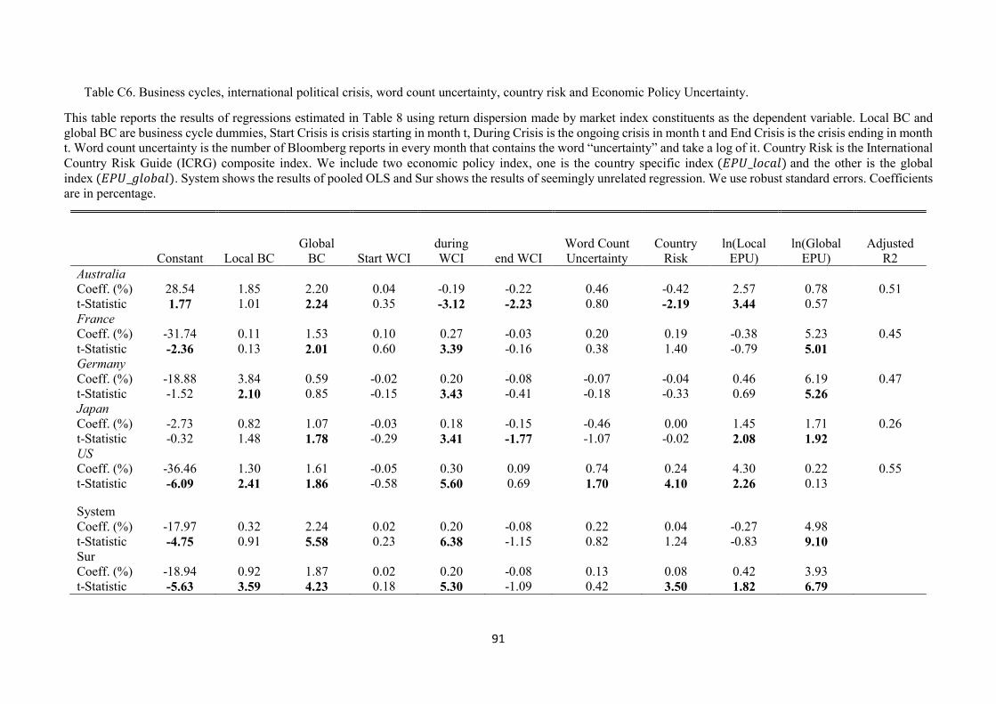
91
Table C6. Business cycles, international political crisis, word count uncertainty, country risk and Economic Policy Uncertainty.
This table reports the results of regressions estimated in Table 8 using return dispersion made by market index constituents as the dependent variable. Local BC and
global BC are business cycle dummies, Start Crisis is crisis starting in month t, During Crisis is the ongoing crisis in month t and End Crisis is the crisis ending in month
t. Word count uncertainty is the number of Bloomberg reports in every month that contains the word “uncertainty” and take a log of it. Country Risk is the International
Country Risk Guide (ICRG) composite index. We include two economic policy index, one is the country specific index (𝐸𝑃𝑈_𝑙𝑜𝑐𝑎𝑙) and the other is the global
index (𝐸𝑃𝑈_𝑔𝑙𝑜𝑏𝑎𝑙). System shows the results of pooled OLS and Sur shows the results of seemingly unrelated regression. We use robust standard errors. Coefficients
are in percentage.
Constant Local BC
Global
BC Start WCI
during
WCI end WCI
Word Count
Uncertainty
Country
Risk
ln(Local
EPU)
ln(Global
EPU)
Adjusted
R2
Australia Coeff. (%) 28.54 1.85 2.20 0.04 -0.19 -0.22 0.46 -0.42 2.57 0.78 0.51
t-Statistic 1.77 1.01 2.24 0.35 -3.12 -2.23 0.80 -2.19 3.44 0.57 France Coeff. (%) -31.74 0.11 1.53 0.10 0.27 -0.03 0.20 0.19 -0.38 5.23 0.45
t-Statistic -2.36 0.13 2.01 0.60 3.39 -0.16 0.38 1.40 -0.79 5.01 Germany Coeff. (%) -18.88 3.84 0.59 -0.02 0.20 -0.08 -0.07 -0.04 0.46 6.19 0.47
t-Statistic -1.52 2.10 0.85 -0.15 3.43 -0.41 -0.18 -0.33 0.69 5.26 Japan Coeff. (%) -2.73 0.82 1.07 -0.03 0.18 -0.15 -0.46 0.00 1.45 1.71 0.26
t-Statistic -0.32 1.48 1.78 -0.29 3.41 -1.77 -1.07 -0.02 2.08 1.92 US Coeff. (%) -36.46 1.30 1.61 -0.05 0.30 0.09 0.74 0.24 4.30 0.22 0.55
t-Statistic -6.09 2.41 1.86 -0.58 5.60 0.69 1.70 4.10 2.26 0.13
System Coeff. (%) -17.97 0.32 2.24 0.02 0.20 -0.08 0.22 0.04 -0.27 4.98 t-Statistic -4.75 0.91 5.58 0.23 6.38 -1.15 0.82 1.24 -0.83 9.10 Sur Coeff. (%) -18.94 0.92 1.87 0.02 0.20 -0.08 0.13 0.08 0.42 3.93 t-Statistic -5.63 3.59 4.23 0.18 5.30 -1.09 0.42 3.50 1.82 6.79
Related Documents