Macro policy reform, labour market, poverty and inequality in urban Ethiopia: a Micro-simulation approach

Macro Policy Reform, Labour Market, Poverty & Inequality in Urban Ethiopia: A Micro-simulation

Approach

Alemayehu Geda

Alem Abereha

Final Report of Phase II AERC Project on

“Poverty, Income Distribution and Labour Market Issues in Ethiopia”

February, 2006

alemahyew

Draft

alemahyew

For Comment

Macro Policy, Labour Market and Poverty in Ethiopia Alemayehu and Alem 2

Macro Policy Reform, Labour Market, Poverty & Inequality in Urban Ethiopia: A Microsimulation Approach

Alemayehu Geda

Alem Abereha

I. INTRODUCTION Governments in Africa and their development partners such as the Worland Band and IMF are concerned with the issue of reducing poverty. Thus, since the 1980 they have deployed macro policy packages that are believed to help in addressing the challenge of reducing poverty. This took the form of Structural Adjustment Packages (SAP) in the 1980s and 1990s and now taking a ‘new’ form called Poverty Reductions Strategy Programs/Papers (PRSPs) or its new (or competitive version) ‘the Millennium Development Goals’ (MDGs). At the heart of these policy packages lie a set of macro polices, which can loosely be termed as ‘liberalization and conservative monetary and fiscal policies’ – or reform in short, that are believe to help the fight against poverty. One important analytical shortcoming of these efforts is lack of a link between macro policies employed and indicators of issues of poverty and inequality. In other words, we do not precisely know through which channels the deployed macro policies are supposed to affect poverty (perhaps the only exception being the presumption that stable macro environment is good for growth and hence for reducing poverty). One obvious channels through which macro polices may affect poverty is through its effect on the labour market and hence earnings form that market. Thus, characterization of the labour market in general and modelling how incomes are generated in this market in particular are key to understand the propagation mechanisms through which macro polices may affect poverty and inequality. This paper is aimed at exploring this issue using the Ethiopian household data and a micro simulation technique. The rest of the study is organized as follows. Following a brief review of the macroeconomic performance in post-reform Ethiopia in the next sub-section, in section two we will analyze the structure of employment and household income in urban Ethiopia using two household data (of 1994 and 2004) and exploratory data analysis. In section three we will specify the models employed in the study and estimate their parameters. Using these models we have made a microsimulation analysis of the impact of the reform on poverty and inequality in the same section. Section four will conclude the paper.

1.1 The 1992 Macro Policy Reform and Poverty

In 1991 the rebel forces (The Ethiopian People Revolutionary Democratic Front, EPRDF) overturned the ‘socialist’ military regime that ruled the country for a brutal 17 years. With the


support of the Bretoon Wood institutions, the new regime began to carry out a liberalization policy in a typical Structural Adjustment Programme (SAPs) fashion. In terms of economic policy, this period witnessed a marked departure from the ‘Socialist’ control regime of the military era – the ‘Derg regime’. The policy reform carried out includes:

a) Financial sector and labour market liberalization

b) Domestic and external trade liberalization

c) Liberalization of the product market, in particular the agricultural sector

d) Pursuing conservative fiscal and monetary policy: expenditure reduction and switching, tax reform, tight monetary policy, exchange rate and public sector reform.

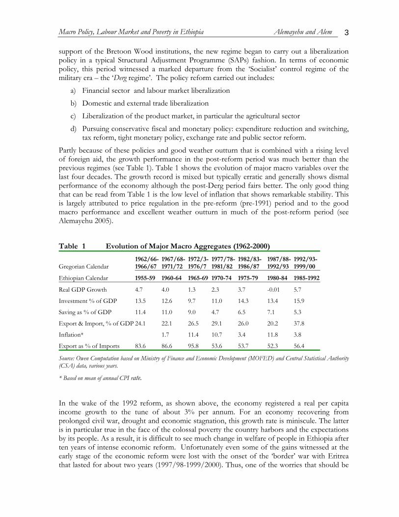
Partly because of these policies and good weather outturn that is combined with a rising level of foreign aid, the growth performance in the post-reform period was much better than the previous regimes (see Table 1). Table 1 shows the evolution of major macro variables over the last four decades. The growth record is mixed but typically erratic and generally shows dismal performance of the economy although the post-Derg period fairs better. The only good thing that can be read from Table 1 is the low level of inflation that shows remarkable stability. This is largely attributed to price regulation in the pre-reform (pre-1991) period and to the good macro performance and excellent weather outturn in much of the post-reform period (see Alemayehu 2005).

Table 1 Evolution of Major Macro Aggregates (1962-2000)

Gregorian Calendar 1962/66-1966/67

1967/68-1971/72

1972/3-1976/7

1977/78-1981/82

1982/83-1986/87

1987/88-1992/93

1992/93-1999/00

Ethiopian Calendar 1955-59 1960-64 1965-69 1970-74 1975-79 1980-84 1985-1992

Real GDP Growth 4.7 4.0 1.3 2.3 3.7 -0.01 5.7

Investment % of GDP 13.5 12.6 9.7 11.0 14.3 13.4 15.9

Saving as % of GDP 11.4 11.0 9.0 4.7 6.5 7.1 5.3

Export & Import, % of GDP 24.1 22.1 26.5 29.1 26.0 20.2 37.8

Inflation* 1.7 11.4 10.7 3.4 11.8 3.8

Export as % of Imports 83.6 86.6 95.8 53.6 53.7 52.3 56.4

Source: Owen Computation based on Ministry of Finance and Economic Development (MOFED) and Central Statistical Authority (CSA) data, various years.

* Based on mean of annual CPI rate.

In the wake of the 1992 reform, as shown above, the economy registered a real per capita income growth to the tune of about 3% per annum. For an economy recovering from prolonged civil war, drought and economic stagnation, this growth rate is miniscule. The latter is in particular true in the face of the colossal poverty the country harbors and the expectations by its people. As a result, it is difficult to see much change in welfare of people in Ethiopia after ten years of intense economic reform. Unfortunately even some of the gains witnessed at the early stage of the economic reform were lost with the onset of the ‘border’ war with Eritrea that lasted for about two years (1997/98-1999/2000). Thus, one of the worries that should be


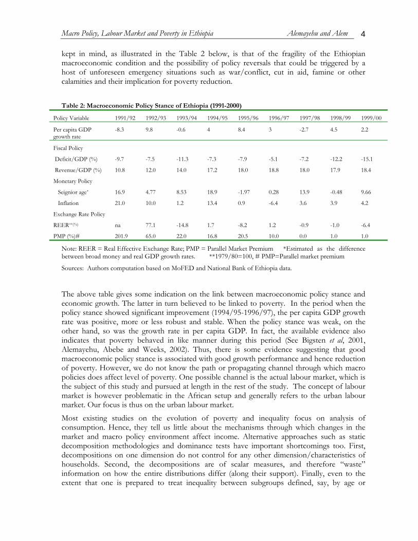
kept in mind, as illustrated in the Table 2 below, is that of the fragility of the Ethiopian macroeconomic condition and the possibility of policy reversals that could be triggered by a host of unforeseen emergency situations such as war/conflict, cut in aid, famine or other calamities and their implication for poverty reduction.

Table 2: Macroeconomic Policy Stance of Ethiopia (1991-2000)

Policy Variable 1991/92 1992/93 1993/94 1994/95 1995/96 1996/97 1997/98 1998/99 1999/00

Per capita GDP growth rate

-8.3 9.8 -0.6 4 8.4 3 -2.7 4.5 2.2

Fiscal Policy

Deficit/GDP (%)

Revenue/GDP (%)

-9.7

10.8

-7.5

12.0

-11.3

14.0

-7.3

17.2

-7.9

18.0

-5.1

18.8

-7.2

18.0

-12.2

17.9

-15.1

18.4

Monetary Policy

Seignior age*

Inflation

16.9

21.0

4.77

10.0

8.53

1.2

18.9

13.4

-1.97

0.9

0.28

-6.4

13.9

3.6

-0.48

3.9

9.66

4.2

Exchange Rate Policy

REER**(%)

PMP (%)#

na

201.9

77.1

65.0

-14.8

22.0

1.7

16.8

-8.2

20.5

1.2

10.0

-0.9

0.0

-1.0

1.0

-6.4

1.0

Note: REER = Real Effective Exchange Rate; PMP = Parallel Market Premium *Estimated as the difference between broad money and real GDP growth rates. **1979/80=100, # PMP=Parallel market premium

Sources: Authors computation based on MoFED and National Bank of Ethiopia data.

The above table gives some indication on the link between macroeconomic policy stance and economic growth. The latter in turn believed to be linked to poverty. In the period when the policy stance showed significant improvement (1994/95-1996/97), the per capita GDP growth rate was positive, more or less robust and stable. When the policy stance was weak, on the other hand, so was the growth rate in per capita GDP. In fact, the available evidence also indicates that poverty behaved in like manner during this period (See Bigsten et al, 2001, Alemayehu, Abebe and Weeks, 2002). Thus, there is some evidence suggesting that good macroeconomic policy stance is associated with good growth performance and hence reduction of poverty. However, we do not know the path or propagating channel through which macro policies does affect level of poverty. One possible channel is the actual labour market, which is the subject of this study and pursued at length in the rest of the study. The concept of labour market is however problematic in the African setup and generally refers to the urban labour market. Our focus is thus on the urban labour market.

Most existing studies on the evolution of poverty and inequality focus on analysis of consumption. Hence, they tell us little about the mechanisms through which changes in the market and macro policy environment affect income. Alternative approaches such as static decomposition methodologies and dominance tests have important shortcomings too. First, decompositions on one dimension do not control for any other dimension/characteristics of households. Second, the decompositions are of scalar measures, and therefore “waste” information on how the entire distributions differ (along their support). Finally, even to the extent that one is prepared to treat inequality between subgroups defined, say, by age or


education, as being driven by those attributes – rather than by correlates – the share of total inequality attributed to that partition tells us nothing of whether it is the distribution of the characteristics (or asset), or the structure of its returns that matters.

In this study, we adopt a microsimulation methodology that does not suffer any of the aforementioned shortcomings. Using this methodology, we will analyze the evolution of poverty and inequality in urban Ethiopia using two sets of surveys. The first is a household survey conducted in seven urban centers in Ethiopia conducted in 1994 and 2000; and the second is a household survey conducted in 15 rural villages in the same years. Hence, we will be able to compare the effects of major policy changes that occurred in the 1990s by comparing the structure of household incomes in 1994 with the structure that prevailed 5-6 years later to detect and explain the major shifts in structure of incomes, which we have hypothesized to be linked with SAPs.

II. THE URBAN LABOUR MARKET, POVERTY AND INEQUALITY IN ETIOPIA: We begin from the working hypothesis that changes in poverty and inequality is likely to be closely associated with changes in the labour market condition. Thus, understanding the labour market helps to identify the channels through which macro policies may affect earnings from the labour market which in turn affect conditions of poverty and inequality. The basic idea of the microsimulation is to isolate the effect of each of the main determinants of the changes in poverty and inequality and associate these changes to the process of macroeconomic adjustment and stabilization, and to the set of liberalization policies which we loosely termed as ‘macro policy reform’. The methodology consists of creating a counterfactual in the form of labour market parameters representing, among other, the employment and remuneration structure, which would prevail if the labour market structure would be different than observed in the year that we take as a point of departure for the analysis (cf. Paes de Barros and Leite 1998; Paes de Barros 1999 cited in Vos and Taylor, 2002; Frenkel and González 1999, Vos and Taylor 2002). This counterfactual may be obtained by either model simulations to generate a case of ‘with-and-without’ or by taking the structure prevailing in another year and imposing it on another. Following the latter approach, we take the Ethiopian micro data of one year, 2000, and simulate what poverty and inequality would have been, had the labour market structure remained what it was in 1994. The two years are selected based on availability of household data in years close to the beginning of the reform period which is the year 1992 and as recently as possible so as to see the effect of these reforms on poverty and inequality.

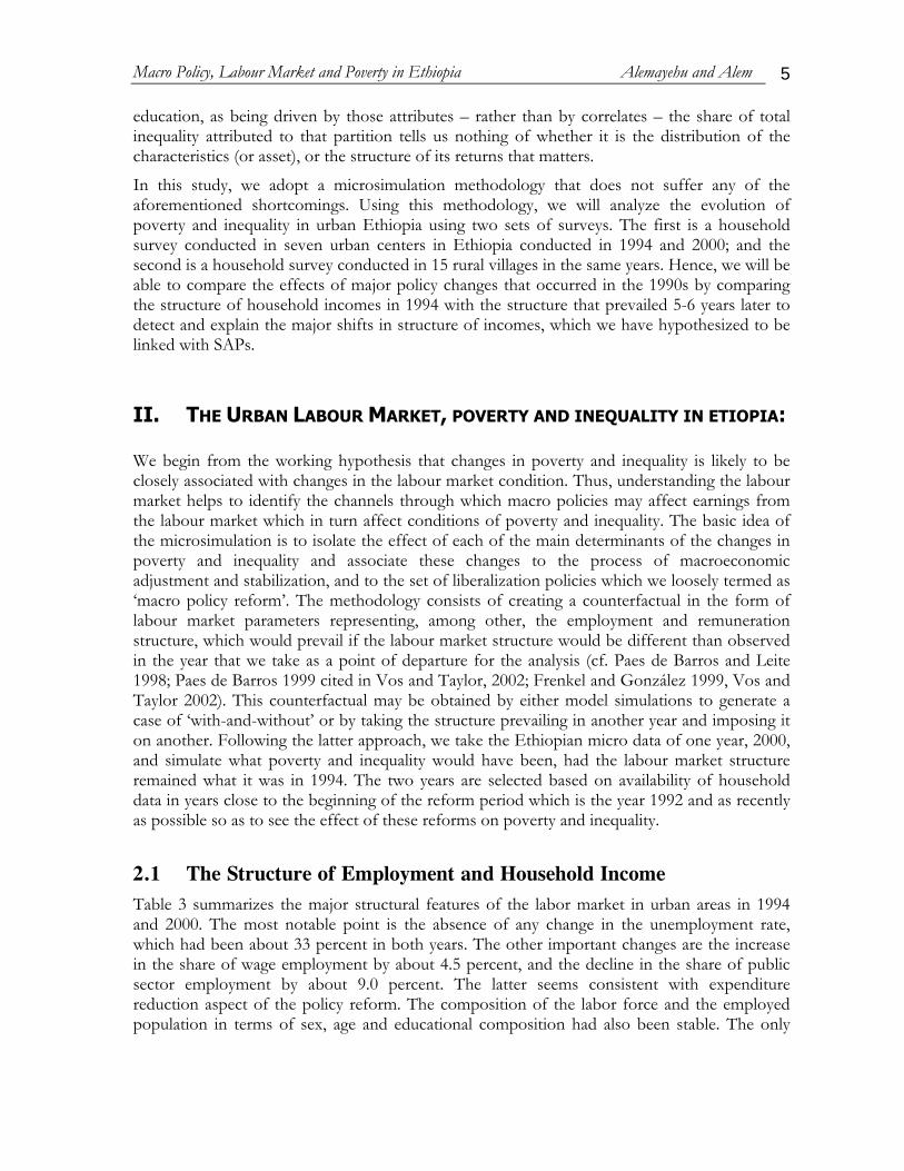
2.1 The Structure of Employment and Household Income Table 3 summarizes the major structural features of the labor market in urban areas in 1994 and 2000. The most notable point is the absence of any change in the unemployment rate, which had been about 33 percent in both years. The other important changes are the increase in the share of wage employment by about 4.5 percent, and the decline in the share of public sector employment by about 9.0 percent. The latter seems consistent with expenditure reduction aspect of the policy reform. The composition of the labor force and the employed population in terms of sex, age and educational composition had also been stable. The only


exception is the decline in the share of persons with no education, by 3 percentage points in the labor force and 6 percentage points among the employed.

Table 3 Characteristics of the labor market: 1994 and 2000 (households)

1994 2000

Percent able-bodied 61.81 65.88

Participation rate 57 53.72

Unemployment rate 33.03 32.93

Self-employment rate 19.34 14.87

of which Female HH. 37.97 37.27

Wage-employment rate 47.63 52.2

of which: Public sector 52.57 43.52

Table 4 Characteristics of the labor force: 1994 and 2000

Economically Active Employed

1994 2000 1994 2000

Education

None 32.3 29.01 42.3 36.09

Primary 9.95 10.89 10.67 10.99

Jun. sec. 15.33 16.7 13.42 14.31

Sen. Sec. 29.94 32.39 18.45 25.3

Post-sec. 12.48 11.02 15.16 13.31

Age-group

15_24 32.91 31.44 18.63 19.25

25_34 27.93 30.49 27.8 28.93

35_44 19.54 19.27 25.7 25.81

45_54 12.24 11.7 17.32 15.83

55_64 4.74 4.6 6.71 6.45

Sex

Female 46.83 45.03 45.48 44.15

Male 53.17 54.97 54.52 55.85

Table 5 shows the distribution of households by source of income. The share of households that had income from wage employment increased from about 63 percent to about 68 percent, while the share that had self-employment income declined from 36 percent to 25 percent. The share of households that received ‘other’ (non-labor) incomes increased from about 45 percent to 52 percent. The share of households that depended on income from ‘wage-employment only’ was about 32 percent in 1994 and about 34 percent in 2000, while the share of those that depended on income from self-employment only declined from about 15 percent to about 9


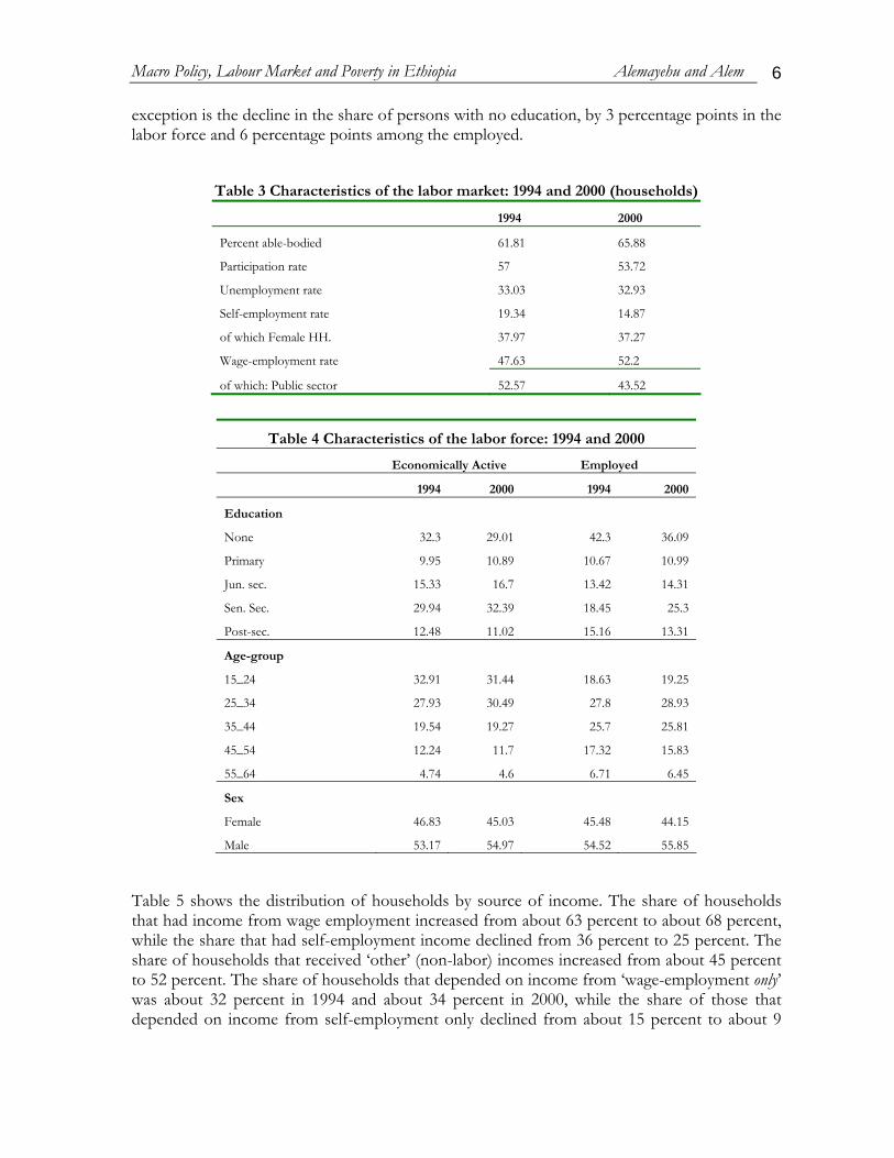
percent. The share of households that depended on ‘other’ incomes was about 13 percent in 1994 and 17 percent in 2000.

Table 5 Sources of household income: 1994 and 2000 1994 2000 Wage-employment income 63.81 67.85 Wage-employment only 32.24 33.86 Self-employment income 35.52 25.43 Self-employment only 14.78 8.96 Other income 45.26 51.65 Other income only 13.27 16.47

Share of households with members working in the wage sector shows almost no change. The share of households with no wage income is slightly lower in 2000 – 34 percent vis-à-vis 38 percent. The share of households with one wage-employed member is about 39 percent in 1994 and 42 percent in 2000, and that of households with two or more wage-employed members is about 24 percent in both years, respectively. Considering all sample households, median household income from wage employment was Birr 144 (per annum) in 1994 and 189 in 2000 and mean income 322 and 379, respectively (the average exchange rate during the period was about $1.00=Birr 8.60). Considering households with positive wage incomes only, median income from wage employment was 350.00 in 1994 and 393 in 2000. The inter-quartile range, an indicator of equality, changed from 471 in 1994 to 526 in 2000.

Median household income from self-employment among households with self-employed members declined by about 39 percent – from Birr 200.00 in 1994 to Birr 123.00 in 2000. The decline was even larger in terms of mean household income from self-employment, which fell by half from Birr 2,476.00 in 1,994 to Birr 1,260.00 in 2,000. The distribution of self-employment income is more skewed to the right than that of wage income, and this concentration of incomes in the lower end increased in 2000. It seems reasonable to infer that the reform period has been strongly associated with negative outcome for self-employed households. We have examined the three categories of income in detail below.

(i) Wage income

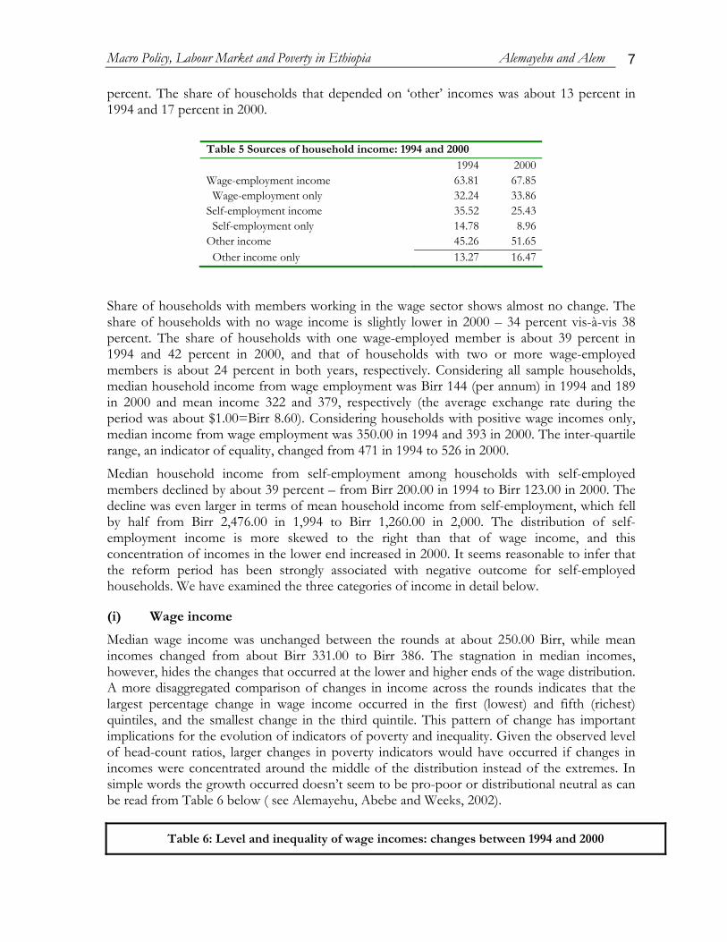
Median wage income was unchanged between the rounds at about 250.00 Birr, while mean incomes changed from about Birr 331.00 to Birr 386. The stagnation in median incomes, however, hides the changes that occurred at the lower and higher ends of the wage distribution. A more disaggregated comparison of changes in income across the rounds indicates that the largest percentage change in wage income occurred in the first (lowest) and fifth (richest) quintiles, and the smallest change in the third quintile. This pattern of change has important implications for the evolution of indicators of poverty and inequality. Given the observed level of head-count ratios, larger changes in poverty indicators would have occurred if changes in incomes were concentrated around the middle of the distribution instead of the extremes. In simple words the growth occurred doesn’t seem to be pro-poor or distributional neutral as can be read from Table 6 below ( see Alemayehu, Abebe and Weeks, 2002).

Table 6: Level and inequality of wage incomes: changes between 1994 and 2000


Gini Mean Median 1994 2000 Change % 1994 2000 Change % 1994 2000 Change %

Q1 30.96 23.71 -7.25 -23.41 42.45 64.11 21.66 51.02 38.44 65.99 27.55 71.66Q2 10.69 10.15 -0.54 -5.04 136.99 146.20 9.21 6.72 134.56 142.99 8.43 6.27Q3 8.95 9.38 0.43 4.81 249.42 254.84 5.41 2.17 250.00 246.50 -3.50 -1.40Q4 8.31 8.75 0.44 5.28 405.55 448.94 43.39 10.70 400.00 441.70 41.70 10.43Q5 23.56 27.10 3.54 15.02 857.08 1025.08 168.00 19.60 689.70 759.49 69.79 10.12

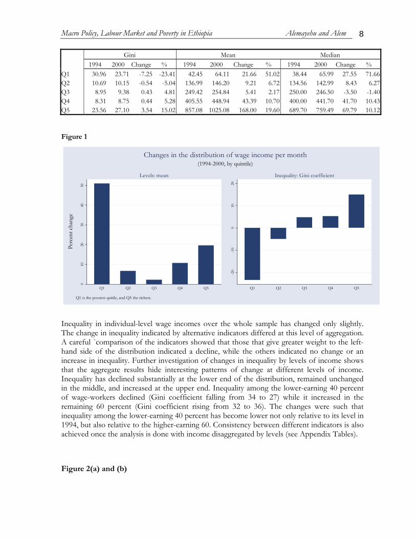
Figure 1

010

2030

4050

Q1 Q2 Q3 Q4 Q5

Levels: mean

-20

-10

010

20

Q1 Q2 Q3 Q4 Q5

Inequality: Gini coefficient

Perc

ent c

hang

e

Q1 is the poorest quitile, and Q5 the richest.

(1994-2000, by quintile)Changes in the distribution of wage income per month

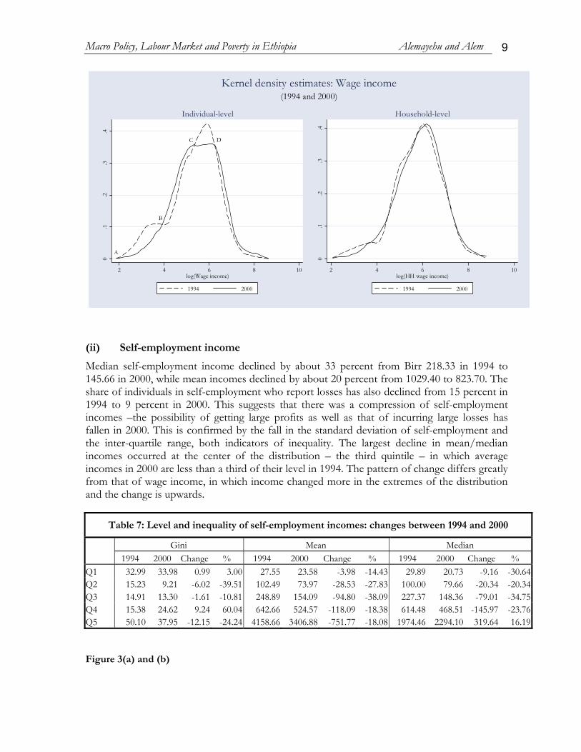
Inequality in individual-level wage incomes over the whole sample has changed only slightly. The change in inequality indicated by alternative indicators differed at this level of aggregation. A careful `comparison of the indicators showed that those that give greater weight to the left-hand side of the distribution indicated a decline, while the others indicated no change or an increase in inequality. Further investigation of changes in inequality by levels of income shows that the aggregate results hide interesting patterns of change at different levels of income. Inequality has declined substantially at the lower end of the distribution, remained unchanged in the middle, and increased at the upper end. Inequality among the lower-earning 40 percent of wage-workers declined (Gini coefficient falling from 34 to 27) while it increased in the remaining 60 percent (Gini coefficient rising from 32 to 36). The changes were such that inequality among the lower-earning 40 percent has become lower not only relative to its level in 1994, but also relative to the higher-earning 60. Consistency between different indicators is also achieved once the analysis is done with income disaggregated by levels (see Appendix Tables).

Figure 2(a) and (b)


A

B

C D

0.1

.2.3

.4

2 4 6 8 10log(Wage income)

1994 2000

Individual-level

0.1

.2.3

.4

2 4 6 8 10log(HH wage income)

1994 2000

Household-level

(1994 and 2000)Kernel density estimates: Wage income

(ii) Self-employment income

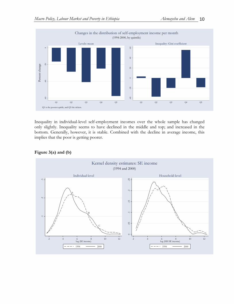
Median self-employment income declined by about 33 percent from Birr 218.33 in 1994 to 145.66 in 2000, while mean incomes declined by about 20 percent from 1029.40 to 823.70. The share of individuals in self-employment who report losses has also declined from 15 percent in 1994 to 9 percent in 2000. This suggests that there was a compression of self-employment incomes –the possibility of getting large profits as well as that of incurring large losses has fallen in 2000. This is confirmed by the fall in the standard deviation of self-employment and the inter-quartile range, both indicators of inequality. The largest decline in mean/median incomes occurred at the center of the distribution – the third quintile – in which average incomes in 2000 are less than a third of their level in 1994. The pattern of change differs greatly from that of wage income, in which income changed more in the extremes of the distribution and the change is upwards.

Table 7: Level and inequality of self-employment incomes: changes between 1994 and 2000


Q1 32.99 33.98 0.99 3.00 27.55 23.58 -3.98 -14.43 29.89 20.73 -9.16 -30.64Q2 15.23 9.21 -6.02 -39.51 102.49 73.97 -28.53 -27.83 100.00 79.66 -20.34 -20.34Q3 14.91 13.30 -1.61 -10.81 248.89 154.09 -94.80 -38.09 227.37 148.36 -79.01 -34.75Q4 15.38 24.62 9.24 60.04 642.66 524.57 -118.09 -18.38 614.48 468.51 -145.97 -23.76Q5 50.10 37.95 -12.15 -24.24 4158.66 3406.88 -751.77 -18.08 1974.46 2294.10 319.64 16.19

Figure 3(a) and (b)


-60

-40

-20

0

Q1 Q2 Q3 Q4 Q5

Levels: mean

-40

-20

020

4060

Q1 Q2 Q3 Q4 Q5

Inequality: Gini coefficientPe

rcen

t cha

nge


(1994-2000, by quintile)Changes in the distribution of self-employment income per month

Inequality in individual-level self-employment incomes over the whole sample has changed only slightly. Inequality seems to have declined in the middle and top; and increased in the bottom. Generally, however, it is stable. Combined with the decline in average income, this implies that the poor is getting poorer.

Figure 3(a) and (b)

A

B

C

.1.2

.3

2 4 6 8 10 12log (SE income)

1994 2000

Individual-level

0.0

5.1

.15

.2.2

5

2 4 6 8 10 12log (HH SE income)

1994 2000

Household-level

(1994 and 2000)Kernel density estimates: SE income


(iii) Other income

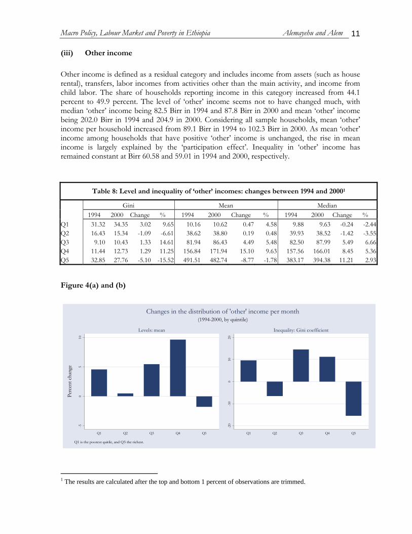
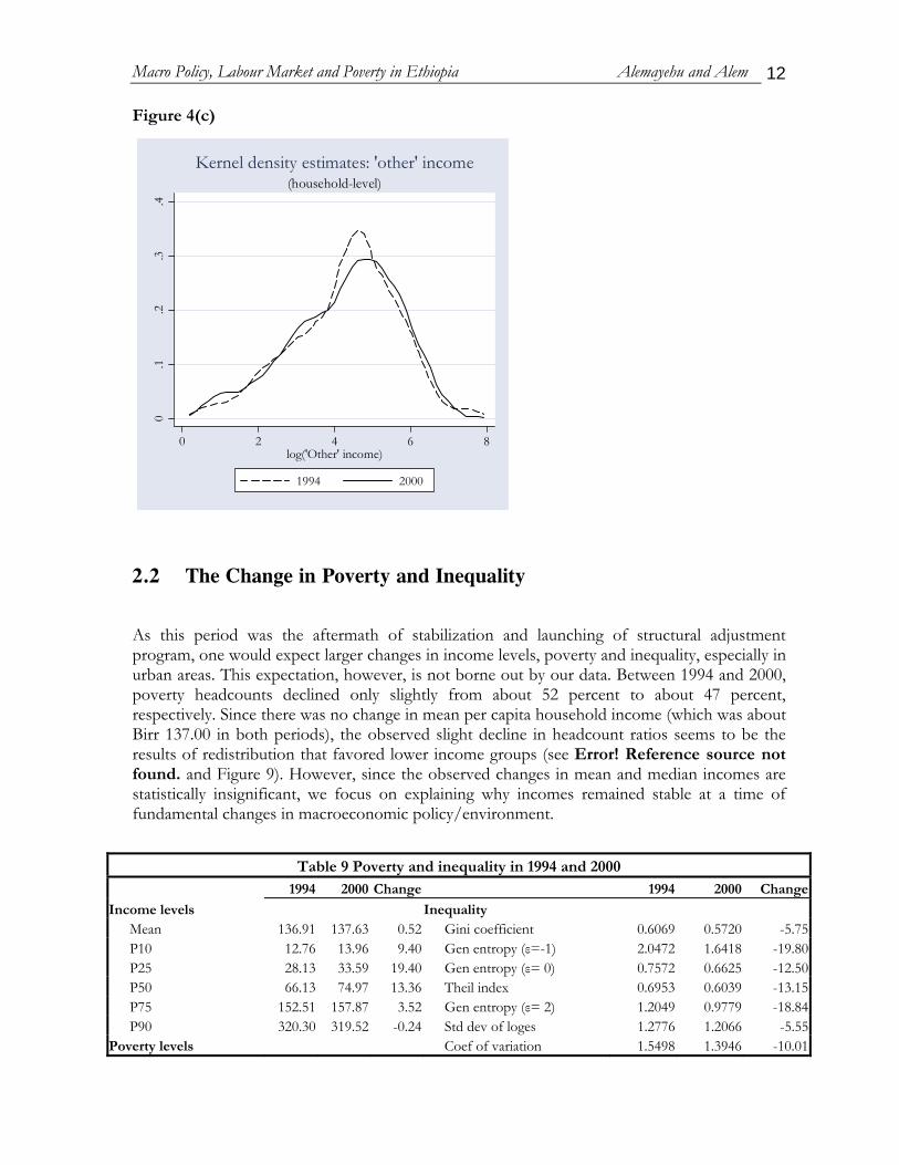
Other income is defined as a residual category and includes income from assets (such as house rental), transfers, labor incomes from activities other than the main activity, and income from child labor. The share of households reporting income in this category increased from 44.1 percent to 49.9 percent. The level of ‘other’ income seems not to have changed much, with median ‘other’ income being 82.5 Birr in 1994 and 87.8 Birr in 2000 and mean ‘other’ income being 202.0 Birr in 1994 and 204.9 in 2000. Considering all sample households, mean ‘other’ income per household increased from 89.1 Birr in 1994 to 102.3 Birr in 2000. As mean ‘other’ income among households that have positive ‘other’ income is unchanged, the rise in mean income is largely explained by the ‘participation effect’. Inequality in ‘other’ income has remained constant at Birr 60.58 and 59.01 in 1994 and 2000, respectively.

Table 8: Level and inequality of ‘other’ incomes: changes between 1994 and 20001


Q1 31.32 34.35 3.02 9.65 10.16 10.62 0.47 4.58 9.88 9.63 -0.24 -2.44Q2 16.43 15.34 -1.09 -6.61 38.62 38.80 0.19 0.48 39.93 38.52 -1.42 -3.55Q3 9.10 10.43 1.33 14.61 81.94 86.43 4.49 5.48 82.50 87.99 5.49 6.66Q4 11.44 12.73 1.29 11.25 156.84 171.94 15.10 9.63 157.56 166.01 8.45 5.36Q5 32.85 27.76 -5.10 -15.52 491.51 482.74 -8.77 -1.78 383.17 394.38 11.21 2.93

Figure 4(a) and (b)

-50

510

Q1 Q2 Q3 Q4 Q5

Levels: mean

-20

-10

010

20

Q1 Q2 Q3 Q4 Q5

Inequality: Gini coefficient

Perc

ent c

hang

e


(1994-2000, by quintile)Changes in the distribution of 'other' income per month

1 The results are calculated after the top and bottom 1 percent of observations are trimmed.


Figure 4(c)

0.1

.2.3

.4

0 2 4 6 8log('Other' income)

1994 2000

(household-level)Kernel density estimates: 'other' income

2.2 The Change in Poverty and Inequality

As this period was the aftermath of stabilization and launching of structural adjustment program, one would expect larger changes in income levels, poverty and inequality, especially in urban areas. This expectation, however, is not borne out by our data. Between 1994 and 2000, poverty headcounts declined only slightly from about 52 percent to about 47 percent, respectively. Since there was no change in mean per capita household income (which was about Birr 137.00 in both periods), the observed slight decline in headcount ratios seems to be the results of redistribution that favored lower income groups (see Error! Reference source not found. and Figure 9). However, since the observed changes in mean and median incomes are statistically insignificant, we focus on explaining why incomes remained stable at a time of fundamental changes in macroeconomic policy/environment.

Table 9 Poverty and inequality in 1994 and 2000

1994 2000 Change 1994 2000 Change

Income levels Inequality Mean 136.91 137.63 0.52 Gini coefficient 0.6069 0.5720 -5.75P10 12.76 13.96 9.40 Gen entropy (ε=-1) 2.0472 1.6418 -19.80P25 28.13 33.59 19.40 Gen entropy (ε= 0) 0.7572 0.6625 -12.50P50 66.13 74.97 13.36 Theil index 0.6953 0.6039 -13.15P75 152.51 157.87 3.52 Gen entropy (ε= 2) 1.2049 0.9779 -18.84P90 320.30 319.52 -0.24 Std dev of loges 1.2776 1.2066 -5.55

Poverty levels Coef of variation 1.5498 1.3946 -10.01


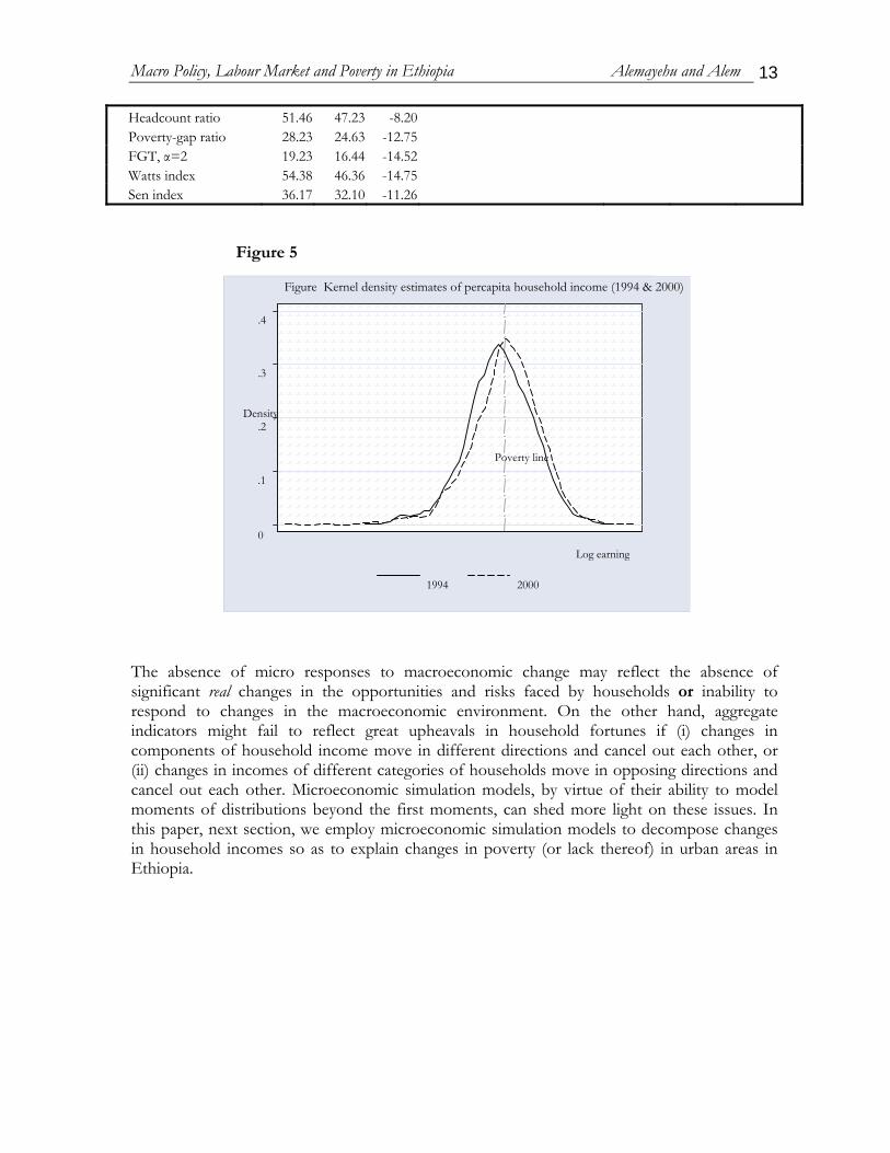
Headcount ratio 51.46 47.23 -8.20 Poverty-gap ratio 28.23 24.63 -12.75 FGT, α=2 19.23 16.44 -14.52 Watts index 54.38 46.36 -14.75 Sen index 36.17 32.10 -11.26

Figure 5

Figure Kernel density estimates of percapita household income (1994 & 2000)

.4

.3

.2 Density

Poverty line

.1

0 Log earning

1994 2000

The absence of micro responses to macroeconomic change may reflect the absence of significant real changes in the opportunities and risks faced by households or inability to respond to changes in the macroeconomic environment. On the other hand, aggregate indicators might fail to reflect great upheavals in household fortunes if (i) changes in components of household income move in different directions and cancel out each other, or (ii) changes in incomes of different categories of households move in opposing directions and cancel out each other. Microeconomic simulation models, by virtue of their ability to model moments of distributions beyond the first moments, can shed more light on these issues. In this paper, next section, we employ microeconomic simulation models to decompose changes in household incomes so as to explain changes in poverty (or lack thereof) in urban areas in Ethiopia.


3 MODELLING THE URBAN LABOUR MARKET AND MICROSIMULATION

RESULTS

3.1 THE MODEL

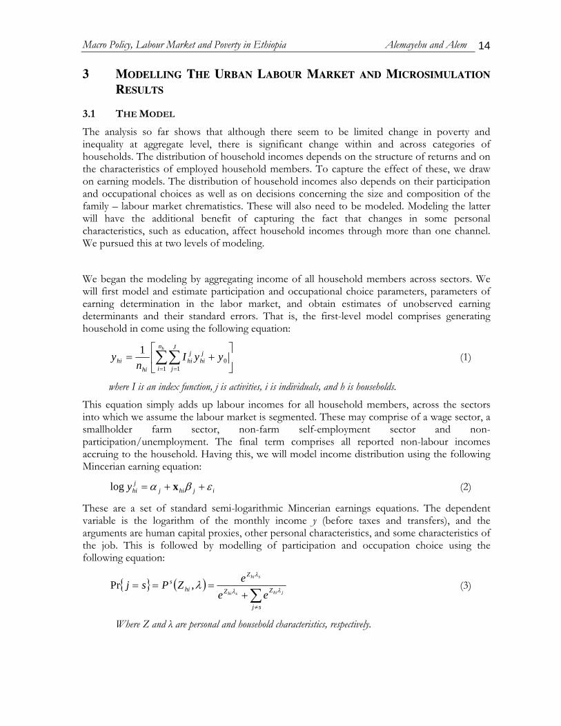
The analysis so far shows that although there seem to be limited change in poverty and inequality at aggregate level, there is significant change within and across categories of households. The distribution of household incomes depends on the structure of returns and on the characteristics of employed household members. To capture the effect of these, we draw on earning models. The distribution of household incomes also depends on their participation and occupational choices as well as on decisions concerning the size and composition of the family – labour market chrematistics. These will also need to be modeled. Modeling the latter will have the additional benefit of capturing the fact that changes in some personal characteristics, such as education, affect household incomes through more than one channel. We pursued this at two levels of modeling.

We began the modeling by aggregating income of all household members across sectors. We will first model and estimate participation and occupational choice parameters, parameters of earning determination in the labor market, and obtain estimates of unobserved earning determinants and their standard errors. That is, the first-level model comprises generating household in come using the following equation:

⎥⎦

⎤⎢⎣

⎡+= ∑∑

= =0

1 1

1 yyIn

yhn

i

J

j

jhi

jhi

hihi (1)

where I is an index function, j is activities, i is individuals, and h is households. This equation simply adds up labour incomes for all household members, across the sectors into which we assume the labour market is segmented. These may comprise of a wage sector, a smallholder farm sector, non-farm self-employment sector and non-participation/unemployment. The final term comprises all reported non-labour incomes accruing to the household. Having this, we will model income distribution using the following Mincerian earning equation:

ijhijj

hiy εβα ++= xlog (2)

These are a set of standard semi-logarithmic Mincerian earnings equations. The dependent variable is the logarithm of the monthly income y (before taxes and transfers), and the arguments are human capital proxies, other personal characteristics, and some characteristics of the job. This is followed by modelling of participation and occupation choice using the following equation:

{ } ( )∑≠

+===

sj

ZZ

Z

his

jhishi

shi

eeeZPsj λλ

λ

λ,Pr (3)

Where Z and λ are personal and household characteristics, respectively.


This block models the choice of occupation (into wage employment, smallholder farming, non-farm self-employment, or inactivity) by means of a discrete choice model –specifically, a multinomial logit – which estimates the probability of choice of each occupation as a function of a set of regional, family and personal variables characteristics

3.2 ESTIMATED RESULTS

Determination of earnings

The first set of equations in our model includes two standard semi-logarithmic Mincerian earnings equations, one for the self-employed and another for the wage employed. The form of the earnings equations given as equation (2) above is used:

ijhijj

hiy εβα ++= xlog

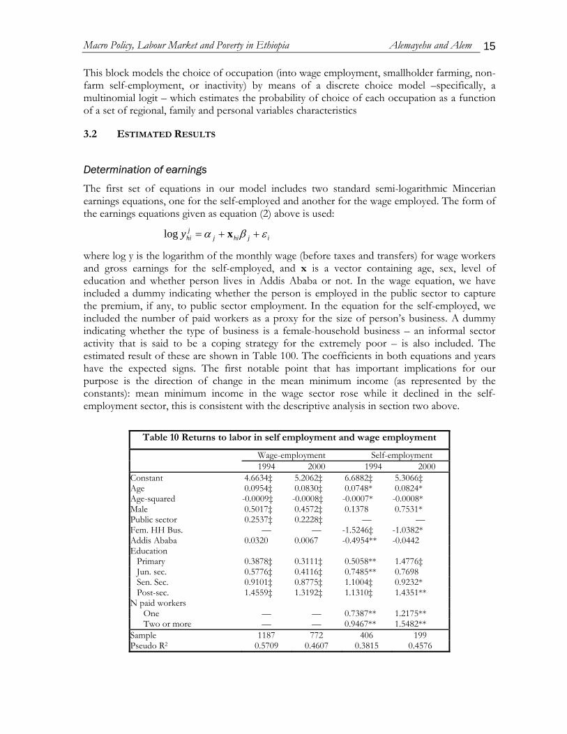
where log y is the logarithm of the monthly wage (before taxes and transfers) for wage workers and gross earnings for the self-employed, and x is a vector containing age, sex, level of education and whether person lives in Addis Ababa or not. In the wage equation, we have included a dummy indicating whether the person is employed in the public sector to capture the premium, if any, to public sector employment. In the equation for the self-employed, we included the number of paid workers as a proxy for the size of person’s business. A dummy indicating whether the type of business is a female-household business – an informal sector activity that is said to be a coping strategy for the extremely poor – is also included. The estimated result of these are shown in Table 100. The coefficients in both equations and years have the expected signs. The first notable point that has important implications for our purpose is the direction of change in the mean minimum income (as represented by the constants): mean minimum income in the wage sector rose while it declined in the self-employment sector, this is consistent with the descriptive analysis in section two above.

Table 10 Returns to labor in self employment and wage employment

Wage-employment Self-employment 1994 2000 1994 2000 Constant 4.6634‡ 5.2062‡ 6.6882‡ 5.3066‡ Age 0.0954‡ 0.0830‡ 0.0748* 0.0824* Age-squared -0.0009‡ -0.0008‡ -0.0007* -0.0008* Male 0.5017‡ 0.4572‡ 0.1378 0.7531* Public sector 0.2537‡ 0.2228‡ — — Fem. HH Bus. — — -1.5246‡ -1.0382* Addis Ababa 0.0320 0.0067 -0.4954** -0.0442 Education

Primary 0.3878‡ 0.3111‡ 0.5058** 1.4776‡ Jun. sec. 0.5776‡ 0.4116‡ 0.7485** 0.7698 Sen. Sec. 0.9101‡ 0.8775‡ 1.1004‡ 0.9232* Post-sec. 1.4559‡ 1.3192‡ 1.1310‡ 1.4351**

N paid workers One — — 0.7387** 1.2175** Two or more — — 0.9467** 1.5482**

Sample 1187 772 406 199 Pseudo R2 0.5709 0.4607 0.3815 0.4576


Note * p<0.05; ** p<0.01; ‡ p<0.001

In the wage sector, there has been a decline between the years in the premiums associated with being male, being a public-sector employee as well the premiums associated with experience and the level of education. This may relate to the lack of incentive-compatible pay system in public sector. In the self-employment sector, the disadvantages arising from operating being female household businesses have become bigger, while the premiums associated with larger business have increased substantially. The effect of being male, which was insignificant in 1994, had become positive in 2000. If female-headed business is a good proxy for the poor in the informal sector, the reform is associated with relative negative outcome for this group. The effect of residence in Addis Ababa turned insignificant in 2000 from having a negative effect in 1994.

Participation and occupational choice

The choice of occupation (into wage employment, smallholder farming, non-farm self-employment, or inactivity) is modelled by means of a discrete choice model – a multinomial logit – which is given as equation 3 above and reproduced below,

{ } ( )∑≠

+===

sj

ZZ

Z

his

jhishi

shi

eeeZPsj λλ

λ

λ,Pr

Our occupational choice of able-bodied individuals is categorized into four: inactivity, unemployment, self-employment and wage employment. Since inactivity is considered as one choice, this models labour supply of household members as well. The comparison group for our occupational choice model is the able-bodied population that is not economically active. In terms of type of employment, we define non-wage employment as consisting of (i) employers/owners of private businesses; (ii) own-account workers; and (iii) those operating female household businesses. All others employment is considered wage employment.

Labour supply/occupational choice by members is modelled as a function of his/her personal characteristics and some household characteristics. Specifically, the sub-vector of Z containing personal characteristics includes sex, age, educational level, a dummy indicating whether person is head of household or not, a dummy indicating whether person is the spouse of the head of household or not, and a dummy indicating whether the person is a student or not. The household characteristics sub-vector contains a dummy indicating whether head of the household is employed or not and the share of employed household members (excluding the person). The resulting estimated equation is shown in Table 11. The significance level and the sign of the coefficients in the two rounds are generally similar, but there is a difference in the magnitude of the coefficients. The result generally shows that the choice of wage employment is largely determined by educational characteristic. It can also be read from Table 11 that, once a household is in school he/she is engaged either in wage employment or is unemployed – showing the absence of limited relationship between schooling and self-employment.


Table 11 Occupational choice model Unemployment Self-employment Wage employment 1994 2000 1994 2000 1994 2000

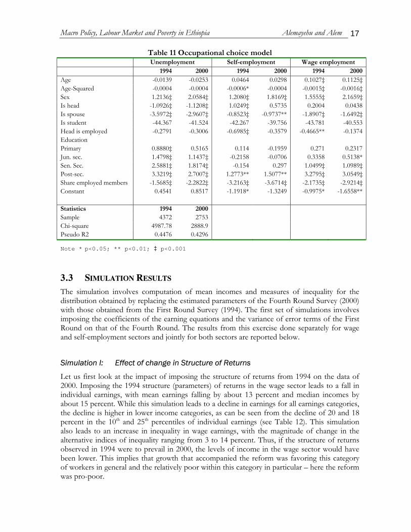
Age -0.0139 -0.0253 0.0464 0.0298 0.1027‡ 0.1125‡Age-Squared -0.0004 -0.0004 -0.0006* -0.0004 -0.0015‡ -0.0016‡Sex 1.2136‡ 2.0584‡ 1.2080‡ 1.8169‡ 1.5555‡ 2.1659‡Is head -1.0926‡ -1.1208‡ 1.0249‡ 0.5735 0.2004 0.0438Is spouse -3.5972‡ -2.9607‡ -0.8523‡ -0.9737** -1.8907‡ -1.6492‡Is student -44.367 -41.524 -42.267 -39.756 -43.781 -40.553Head is employed -0.2791 -0.3006 -0.6985‡ -0.3579 -0.4665** -0.1374Education Primary 0.8880‡ 0.5165 0.114 -0.1959 0.271 0.2317Jun. sec. 1.4798‡ 1.1437‡ -0.2158 -0.0706 0.3358 0.5138*Sen. Sec. 2.5881‡ 1.8174‡ -0.154 0.297 1.0499‡ 1.0989‡Post-sec. 3.3219‡ 2.7007‡ 1.2773** 1.5077** 3.2795‡ 3.0549‡Share employed members -1.5685‡ -2.2822‡ -3.2163‡ -3.6714‡ -2.1735‡ -2.9214‡Constant 0.4541 0.8517 -1.1918* -1.3249 -0.9975* -1.6558** Statistics 1994 2000 Sample 4372 2753 Chi-square 4987.78 2888.9 Pseudo R2 0.4476 0.4296

Note * p<0.05; ** p<0.01; ‡ p<0.001

3.3 SIMULATION RESULTS The simulation involves computation of mean incomes and measures of inequality for the distribution obtained by replacing the estimated parameters of the Fourth Round Survey (2000) with those obtained from the First Round Survey (1994). The first set of simulations involves imposing the coefficients of the earning equations and the variance of error terms of the First Round on that of the Fourth Round. The results from this exercise done separately for wage and self-employment sectors and jointly for both sectors are reported below.

Simulation I: Effect of change in Structure of Returns

Let us first look at the impact of imposing the structure of returns from 1994 on the data of 2000. Imposing the 1994 structure (parameters) of returns in the wage sector leads to a fall in individual earnings, with mean earnings falling by about 13 percent and median incomes by about 15 percent. While this simulation leads to a decline in earnings for all earnings categories, the decline is higher in lower income categories, as can be seen from the decline of 20 and 18 percent in the 10th and 25th percentiles of individual earnings (see Table 12). This simulation also leads to an increase in inequality in wage earnings, with the magnitude of change in the alternative indices of inequality ranging from 3 to 14 percent. Thus, if the structure of returns observed in 1994 were to prevail in 2000, the levels of income in the wage sector would have been lower. This implies that growth that accompanied the reform was favoring this category of workers in general and the relatively poor within this category in particular – here the reform was pro-poor.


Imposing the structure (or parameters) of earnings in the self-employment sector from 1994 on the 2000 data has effects that are opposite to what was observed in the wage sector (see Table 12). If the structure of returns observed in 1994 were to prevail in 2000, the levels of income in the self-employment sector would have been higher – with mean income being about 24 percent higher and median income about 46 percent higher. Since relatively higher percentage increments of the self-employment sector occur at lower levels of income, inequality declines. Alternative indicators of inequality show a decline ranging between 2 and 15 percent, with indicators that are more sensitive to changes at the extremes declining by larger magnitudes. Thus, the reform and the accompanied growth were not pro-poor in the self-employment sector.

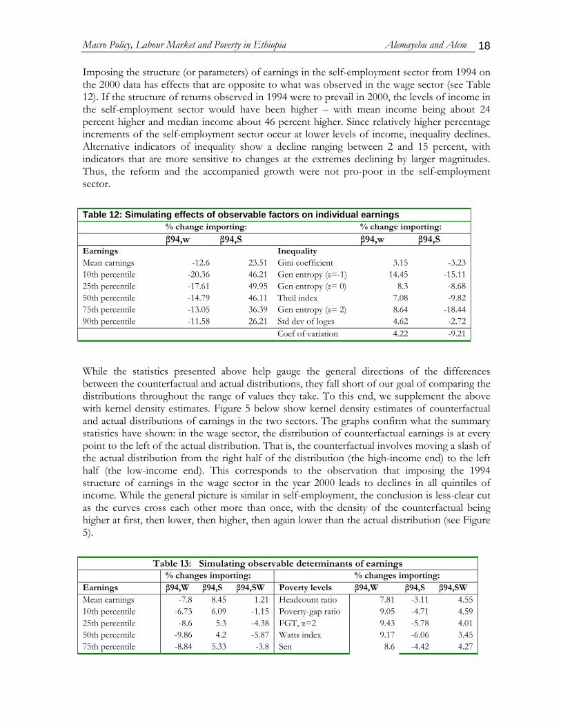
Table 12: Simulating effects of observable factors on individual earnings % change importing: % change importing: β94,w β94,S β94,w β94,S Earnings Inequality Mean earnings -12.6 23.51 Gini coefficient 3.15 -3.2310th percentile -20.36 46.21 Gen entropy (ε=-1) 14.45 -15.1125th percentile -17.61 49.95 Gen entropy (ε= 0) 8.3 -8.6850th percentile -14.79 46.11 Theil index 7.08 -9.8275th percentile -13.05 36.39 Gen entropy (ε= 2) 8.64 -18.4490th percentile -11.58 26.21 Std dev of loges 4.62 -2.72 Coef of variation 4.22 -9.21

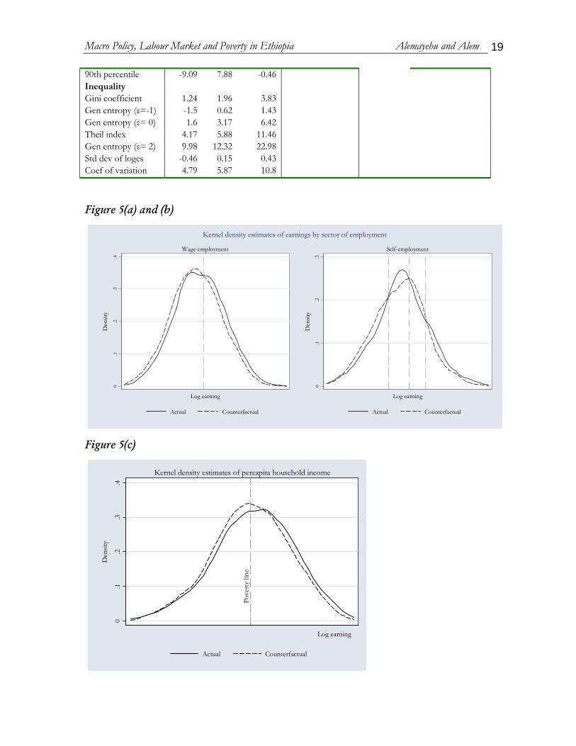
While the statistics presented above help gauge the general directions of the differences between the counterfactual and actual distributions, they fall short of our goal of comparing the distributions throughout the range of values they take. To this end, we supplement the above with kernel density estimates. Figure 5 below show kernel density estimates of counterfactual and actual distributions of earnings in the two sectors. The graphs confirm what the summary statistics have shown: in the wage sector, the distribution of counterfactual earnings is at every point to the left of the actual distribution. That is, the counterfactual involves moving a slash of the actual distribution from the right half of the distribution (the high-income end) to the left half (the low-income end). This corresponds to the observation that imposing the 1994 structure of earnings in the wage sector in the year 2000 leads to declines in all quintiles of income. While the general picture is similar in self-employment, the conclusion is less-clear cut as the curves cross each other more than once, with the density of the counterfactual being higher at first, then lower, then higher, then again lower than the actual distribution (see Figure 5).

Table 13: Simulating observable determinants of earnings

% changes importing: % changes importing: Earnings β94,W β94,S β94,SW Poverty levels β94,W β94,S β94,SW Mean earnings -7.8 8.45 1.21 Headcount ratio 7.81 -3.11 4.5510th percentile -6.73 6.09 -1.15 Poverty-gap ratio 9.05 -4.71 4.5925th percentile -8.6 5.3 -4.38 FGT, α=2 9.43 -5.78 4.0150th percentile -9.86 4.2 -5.87 Watts index 9.17 -6.06 3.4575th percentile -8.84 5.33 -3.8 Sen 8.6 -4.42 4.27


90th percentile -9.09 7.88 -0.46 Inequality Gini coefficient 1.24 1.96 3.83 Gen entropy (ε=-1) -1.5 0.62 1.43 Gen entropy (ε= 0) 1.6 3.17 6.42 Theil index 4.17 5.88 11.46 Gen entropy (ε= 2) 9.98 12.32 22.98 Std dev of loges -0.46 0.15 0.43 Coef of variation 4.79 5.87 10.8

Figure 5(a) and (b)

0.1

.2.3

.4

Den

sity

Log earning

Actual Counterfactual

Wage-employment

0.1

.2.3

Den

sity

Log earning


Self-employment

Kernel density estimates of earnings by sector of employment

Figure 5(c)

Pove

rty li

ne

0.1

.2.3

.4

Den

sity

Log earning


Kernel density estimates of percapita household income


The poverty profiles corresponding to the above two sets of simulations are shown in Table 13. The counterfactual distribution of household incomes provide poverty and inequality indicators consistent with the underlying (counterfactual) distribution of labor incomes. When the structure of returns from the wage sector is imposed alone, mean household incomes fall by about 8 percent and median incomes fall by about 10 percent. Correspondingly, the head count ratio rises by about 8 percent and the other indicators of poverty rise by similar magnitudes. The indicators of inequality did also show increasing inequality, though the magnitudes are smaller. When the 1994 structure of returns for observed factors in self-employment is imposed alone, the level of household incomes rise, indicators of poverty fall, and that of inequality rise.

As these two simulations led to changes in opposite directions, then their effects would cancel each other out if we do them simultaneously. That is what is observed in the last column of Table 13. When the 1994 structure of returns for both sectors is imposed on the condition in the year 2000 simultaneously, the level of incomes declines, but by magnitudes less than when the structure of returns for the wage sector was imposed alone, since part of the negative effect is counteracted by the rise in (counterfactual) self-employment incomes. Poverty is higher, again by magnitudes less than when returns in the wage sector are imposed alone. The effect of changes in the wage sector dominates because wage employment accounts for a much larger share of employment and incomes (is about 60%, see Table 3). The implication for the impact of the liberalization policy is that it favoured the wage earners but not the self-employed, the aggregate effect overall being largely in line with the positive change observed in the wage-earning sector.

Simulation II: Effects of Unobservable Determinants of Earnings

The residuals in Mincerian earnings equations represent returns to labor accountable for unobserved factors that affect wages, and variance of the error terms represent inequality in wages due to these unobserved factors. Running simulations by importing residual variances form 1994 causes almost no change in the level of earnings. Relatively higher effects are observed on the indicators of inequality; with inequality being marginally lower in the counterfactual distribution, however. When the simulation is run using the returns to both observed and unobserved characteristics from 1994, it turns out that the effect of changes in observed characteristics is the dominant cause for any changes between 1994 and 2000. (see Table 16)

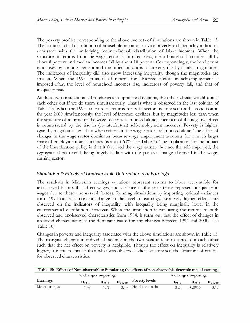
Changes in poverty and inequality associated with the above simulations are shown in Table 15. The marginal changes in individual incomes in the two sectors tend to cancel out each other such that the net effect on poverty is negligible. Though the effect on inequality is relatively higher, it is much smaller than what was observed when we imposed the structure of returns for observed characteristics.

Table 15: Effects of Non-observables: Simulating the effects of non-observable determinants of earning

% changes imposing: % changes imposing: Earnings σ94,w σ94,S σ94,WS

Poverty levels σ94,w σ94,S σ94,WS

Mean earnings 1.37 -1.76 -0.73 Headcount ratio -0.25 -0.0910 -0.17


10th percentile -0.67 0.24 -0.34 Poverty-gap ratio 0.06 -0.0268 -0.3025th percentile -0.08 0.58 0.55 FGT, α=2 0.20 -0.0394 -0.2650th percentile 0.45 0.34 0.23 Watts index 0.10 -0.1425 -0.4375th percentile 0.52 -0.77 0.04 Sen -0.05 -0.0812 -0.2290th percentile 2.57 -1.35 -0.19

Inequality σ94,w σ94,S σ94,WS

Gini coefficient 0.48 -1.0156 -0.70

Gen entropy (ε=-1) 1.24 -3.35 -2.49

Gen entropy (ε= 0) 1.12 -2.08 -1.40

Theil index 0.57 -3.00 -2.33

Gen entropy (ε= 2) -1.20 -6.25 -5.38

Std dev of loges 0.56 -0.67 -0.41

Coef of variation -0.55 -3.02 -2.60

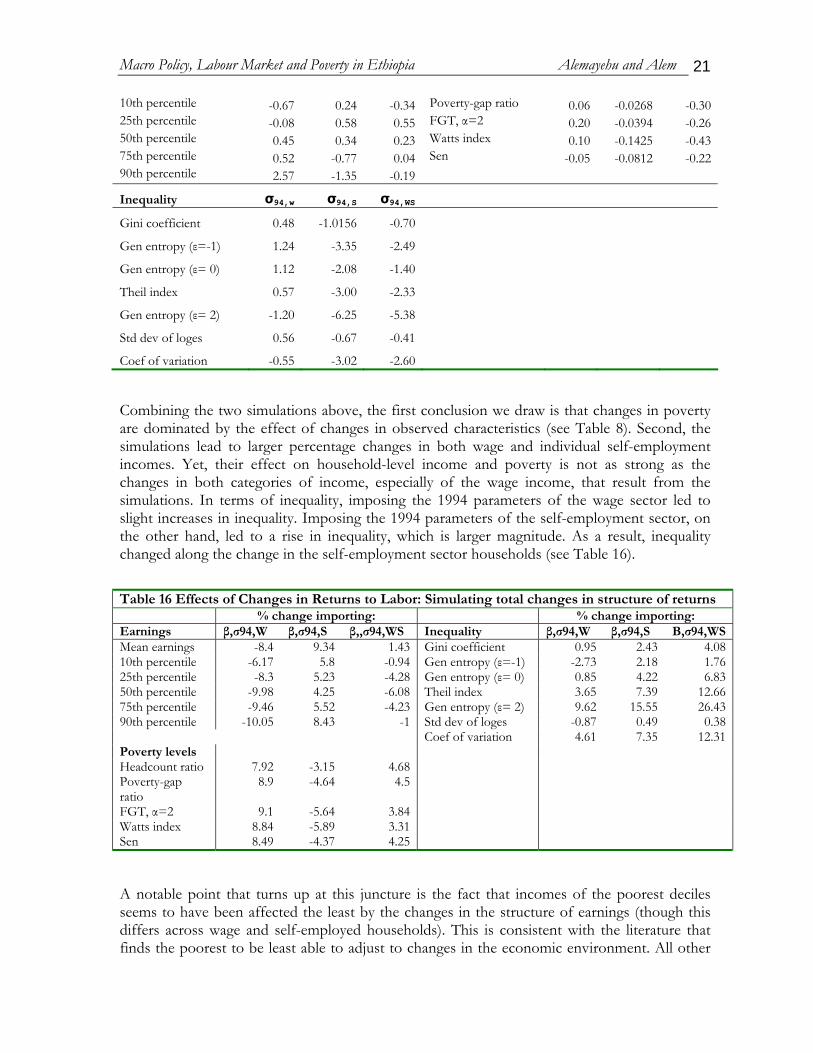
Combining the two simulations above, the first conclusion we draw is that changes in poverty are dominated by the effect of changes in observed characteristics (see Table 8). Second, the simulations lead to larger percentage changes in both wage and individual self-employment incomes. Yet, their effect on household-level income and poverty is not as strong as the changes in both categories of income, especially of the wage income, that result from the simulations. In terms of inequality, imposing the 1994 parameters of the wage sector led to slight increases in inequality. Imposing the 1994 parameters of the self-employment sector, on the other hand, led to a rise in inequality, which is larger magnitude. As a result, inequality changed along the change in the self-employment sector households (see Table 16).

Table 16 Effects of Changes in Returns to Labor: Simulating total changes in structure of returns % change importing: % change importing: Earnings β,σ94,W β,σ94,S β,,σ94,WS Inequality β,σ94,W β,σ94,S Β,σ94,WSMean earnings -8.4 9.34 1.43 Gini coefficient 0.95 2.43 4.0810th percentile -6.17 5.8 -0.94 Gen entropy (ε=-1) -2.73 2.18 1.7625th percentile -8.3 5.23 -4.28 Gen entropy (ε= 0) 0.85 4.22 6.8350th percentile -9.98 4.25 -6.08 Theil index 3.65 7.39 12.6675th percentile -9.46 5.52 -4.23 Gen entropy (ε= 2) 9.62 15.55 26.4390th percentile -10.05 8.43 -1 Std dev of loges -0.87 0.49 0.38 Coef of variation 4.61 7.35 12.31Poverty levels Headcount ratio 7.92 -3.15 4.68 Poverty-gap ratio

8.9 -4.64 4.5

FGT, α=2 9.1 -5.64 3.84 Watts index 8.84 -5.89 3.31 Sen 8.49 -4.37 4.25

A notable point that turns up at this juncture is the fact that incomes of the poorest deciles seems to have been affected the least by the changes in the structure of earnings (though this differs across wage and self-employed households). This is consistent with the literature that finds the poorest to be least able to adjust to changes in the economic environment. All other


income groups seem to have been affected more or less uniformly, with their incomes declining roughly uniformly by about 8 percent when the structure of returns that prevailed in 1994 is imposed.

The second notable point is the fact that the magnitude of change has been very small. Though some fundamental changes in macroeconomic policies and performance are known to have occurred in the 1990’s, their effect on the structure of returns, and hence household welfare, have been, on the average, quite marginal. The indicators of poverty changed by about 6 percent in 6 years – at a rate of less than one percent per year. Headcount ratios have declined less than one-half percentage points per year – a cumulative change of 3.4 percent in six years.

Simulation III: The Effect of Participation and Occupational Choice

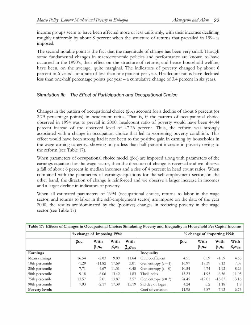
Changes in the pattern of occupational choice (βoc) account for a decline of about 6 percent (or 2.79 percentage points) in headcount ratios. That is, if the pattern of occupational choice observed in 1994 was to prevail in 2000, headcount ratio of poverty would have been 44.44 percent instead of the observed level of 47.23 percent. Thus, the reform was strongly associated with a change in occupation choice that led to worsening poverty condition. This effect would have been strong had it not been to the positive gain in earning by households in the wage earning category, showing only a less than half percent increase in poverty owing to the reform.(see Table 17).

When parameters of occupational choice model (βoc) are imposed along with parameters of the earnings equation for the wage sector, then the direction of change is reversed and we observe a fall of about 6 percent in median incomes and a rise of 4 percent in head count ratios. When combined with the parameters of earnings equations for the self-employment sector, on the other hand, the direction of change is reinforced and we observe a larger increase in incomes and a larger decline in indicators of poverty.

When all estimated parameters of 1994 (occupational choice, returns to labor in the wage sector, and returns to labor in the self-employment sector) are impose on the data of the year 2000, the results are dominated by the (positive) changes in reducing poverty in the wage sector.(see Table 17)

Table 17: Effects of Changes in Occupational Choice: Simulating Poverty and Inequality in Household Per Capita Income

% change of imposing 1994: % change of importing 1994:

βoc With β,σW

With β,σS

With β,σWS

βoc With β,σW

With β,σS

With β,σWS

Earnings Inequality Mean earnings 16.54 -2.83 9.89 11.64 Gini coefficient 4.51 0.59 -1.59 4.6510th percentile -1.29 -11.82 17.69 3.01 Gen entropy (ε=-1) 16.97 18.39 7.13 7.0725th percentile 7.71 -4.67 11.31 -0.48 Gen entropy (ε= 0) 10.54 4.74 -1.92 8.2450th percentile 9.18 -6.06 13.42 1.83 Theil index 13.23 -1.95 -6.56 11.0375th percentile 13.57 2.01 13.87 3.57 Gen entropy (ε= 2) 24.45 -12.01 -15.82 13.1690th percentile 7.93 -2.17 17.39 15.19 Std dev of loges 4.24 5.2 1.18 1.8Poverty levels Coef of variation 11.95 -5.87 -7.93 6.75


Headcount ratio -5.91 4.15 -6.92 -0.44 Poverty-gap ratio -5.52 6.74 -7.71 -3.45 FGT, α=2 -4.62 9.98 -9.12 -4.87 Watts index -4.29 11.52 -8.54 -4.92 Sen -5.2 7.07 -8.01 -2.59

Simulation IV: Effect of Exogenous Variables

In this section, we will attempt to capture the effect of change in the distribution of variables in the right-hand side of the income-determination and occupational-choice equations. The variables are exogenous in the sense that they were not modeled in our set of equations rather than in any structural sense. The first variable in this category is sector of wage employment – public versus private. One of the major concerns during periods of stabilization and structural adjustment involves the effect of lower public sector employment (re-trenchermen of workers) that is not matched by rising employment in the formal private sector. It has been argued that retrenchment in the public sector coupled with lack of productive employment during stabilization and structural adjustment has led not only to higher unemployment but also to increasing ‘informalization’ of the economy. As a large part of the informal sector involves participation in low-productivity/low-remuneration activities, increasing ‘informalization’ is associated with rising poverty.

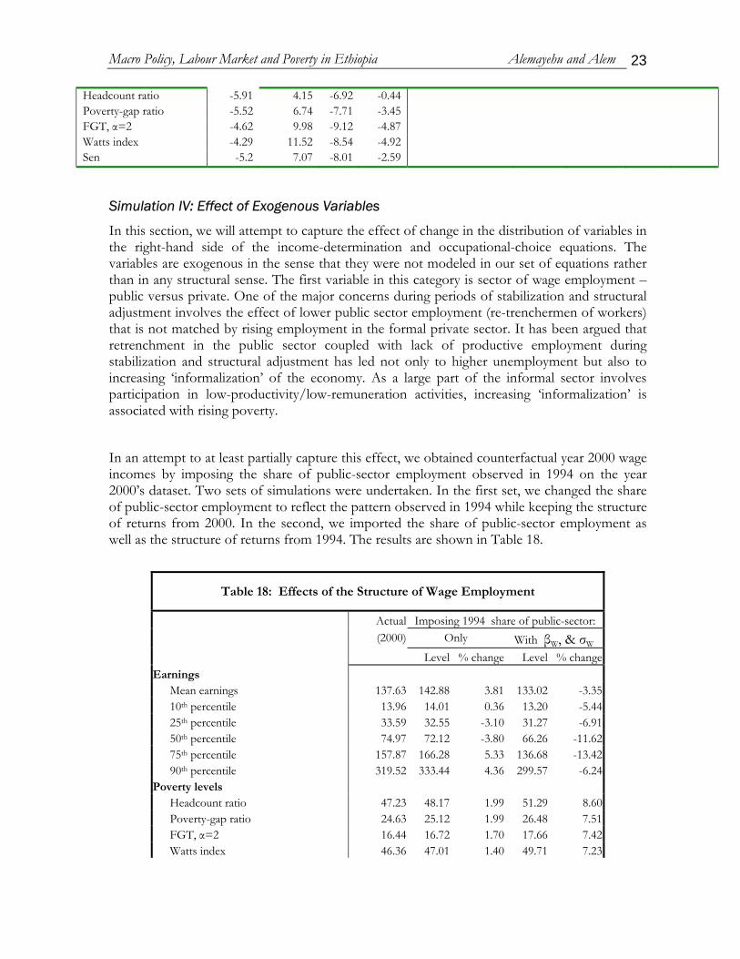
In an attempt to at least partially capture this effect, we obtained counterfactual year 2000 wage incomes by imposing the share of public-sector employment observed in 1994 on the year 2000’s dataset. Two sets of simulations were undertaken. In the first set, we changed the share of public-sector employment to reflect the pattern observed in 1994 while keeping the structure of returns from 2000. In the second, we imported the share of public-sector employment as well as the structure of returns from 1994. The results are shown in Table 18.

Table 18: Effects of the Structure of Wage Employment

Actual Imposing 1994 share of public-sector: (2000) Only With βW, & σW

Level % change Level % changeEarnings

Mean earnings 137.63 142.88 3.81 133.02 -3.3510th percentile 13.96 14.01 0.36 13.20 -5.4425th percentile 33.59 32.55 -3.10 31.27 -6.9150th percentile 74.97 72.12 -3.80 66.26 -11.6275th percentile 157.87 166.28 5.33 136.68 -13.4290th percentile 319.52 333.44 4.36 299.57 -6.24

Poverty levels Headcount ratio 47.23 48.17 1.99 51.29 8.60Poverty-gap ratio 24.63 25.12 1.99 26.48 7.51FGT, α=2 16.44 16.72 1.70 17.66 7.42Watts index 46.36 47.01 1.40 49.71 7.23


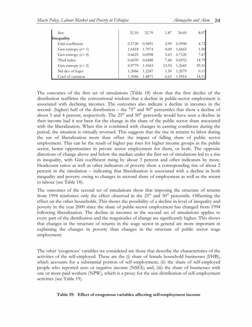
Sen 32.10 32.70 1.87 34.69 8.07Inequality

Gini coefficient 0.5720 0.5891 2.99 0.5990 4.72Gen entropy (ε=-1) 1.6418 1.7074 4.00 1.6665 1.50Gen entropy (ε= 0) 0.6625 0.6998 5.63 0.7120 7.47Theil index 0.6039 0.6488 7.44 0.6932 14.79Gen entropy (ε= 2) 0.9779 1.1043 12.93 1.2645 29.31Std dev of loges 1.2066 1.2247 1.50 1.2079 0.11Coef of variation 1.3946 1.4871 6.63 1.5914 14.11

The outcomes of the first set of simulations (Table 18) show that the first deciles of the distribution reaffirms the conventional wisdom that a decline in public-sector employment is associated with declining incomes. The outcomes also indicate a decline in incomes in the second- (higher) half of the distribution – the 75th and 90th percentiles that show a decline of about 5 and 4 percent, respectively. The 25th and 50th percentile would have seen a decline in their income had it not been for the change in the share of the public sector share associated with the liberalization. When this is combined with changes in earning conditions during the period, the situation is virtually reversed. This suggests that the rise in returns to labor during the ear of liberalization more than offset the impact of falling share of public sector employment. This can be the result of higher pay rises for higher income groups in the public sector, better opportunities in private sector employment for them, or both. The opposite directions of change above and below the median under the first set of simulations led to a rise in inequality, with Gini coefficient rising by about 3 percent and other indicators by more. Headcount ratios as well as other indicators of poverty show a corresponding rise of about 2 percent in the simulation – indicating that liberalization is associated with a decline in both inequality and poverty owing to changes in sectoral share of employment as well as the return to labour (see Table 18).

The outcomes of the second set of simulations show that imposing the structure of returns from 1994 reinforces only the effect observed in the 25th and 50th percentile. Offsetting the effect on the other households. This shows the possibility of a decline in level of inequality and poverty in the year 2000 since the share of public-sector employment has changed from 1994 following liberalization. The decline in incomes in the second set of simulations applies to every part of the distribution and the magnitudes of change are significantly higher. This shows that changes in the structure of returns in the wage sector in general are more important in explaining the changes in poverty than changes in the structure of public sector wage employment.

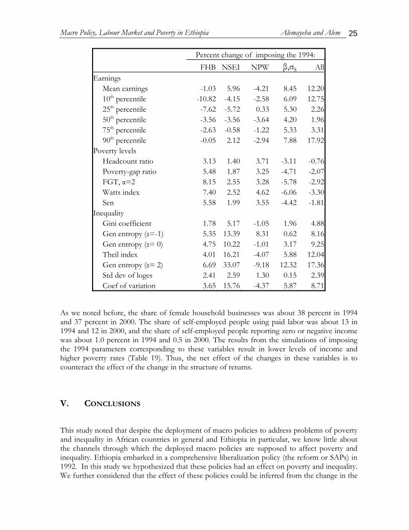
The other ‘exogenous’ variables we considered are those that describe the characteristics of the activities of the self-employed. These are the (i) share of female household businesses (FHB), which accounts for a substantial portion of self-employment; (ii) the share of self-employed people who reported zero or negative income (NSEI); and, (iii) the share of businesses with one or more paid workers (NPW), which is a proxy for the size distribution of self-employment activities (see Table 19).

Table 19: Effect of exogenous variables affecting self-employment income


Percent change of imposing the 1994: FHB NSEI NPW β,σS All Earnings

Mean earnings -1.03 5.96 -4.21 8.45 12.20 10th percentile -10.82 -4.15 -2.58 6.09 12.75 25th percentile -7.62 -5.72 0.33 5.30 2.26 50th percentile -3.56 -3.56 -3.64 4.20 1.96 75th percentile -2.63 -0.58 -1.22 5.33 3.31 90th percentile -0.05 2.12 -2.94 7.88 17.92

Poverty levels Headcount ratio 3.13 1.40 3.71 -3.11 -0.76 Poverty-gap ratio 5.48 1.87 3.25 -4.71 -2.07 FGT, α=2 8.15 2.55 3.28 -5.78 -2.92 Watts index 7.40 2.52 4.62 -6.06 -3.30 Sen 5.58 1.99 3.55 -4.42 -1.81

Inequality Gini coefficient 1.78 5.17 -1.05 1.96 4.88 Gen entropy (ε=-1) 5.35 13.39 8.31 0.62 8.16 Gen entropy (ε= 0) 4.75 10.22 -1.01 3.17 9.25 Theil index 4.01 16.21 -4.07 5.88 12.04 Gen entropy (ε= 2) 6.69 33.07 -9.18 12.32 17.36 Std dev of loges 2.41 2.59 1.30 0.15 2.39 Coef of variation 3.65 15.76 -4.37 5.87 8.71

As we noted before, the share of female household businesses was about 38 percent in 1994 and 37 percent in 2000. The share of self-employed people using paid labor was about 13 in 1994 and 12 in 2000, and the share of self-employed people reporting zero or negative income was about 1.0 percent in 1994 and 0.5 in 2000. The results from the simulations of imposing the 1994 parameters corresponding to these variables result in lower levels of income and higher poverty rates (Table 19). Thus, the net effect of the changes in these variables is to counteract the effect of the change in the structure of returns.

V. CONCLUSIONS

This study noted that despite the deployment of macro policies to address problems of poverty and inequality in African countries in general and Ethiopia in particular, we know little about the channels through which the deployed macro policies are supposed to affect poverty and inequality. Ethiopia embarked in a comprehensive liberalization policy (the reform or SAPs) in 1992. In this study we hypothesized that these policies had an effect on poverty and inequality. We further considered that the effect of these policies could be inferred from the change in the


structure of labour market as it is one of the most important channels through which macro polices may affect poverty and inequality. This underscores the need to examine the letter closely. We have used Ethiopian urban household survey data for the year 1994 and 2000 to address this issue.

As the year 1994 was the aftermath of the period that corresponds to the launching of structural adjustment program of the country, one would expect larger changes in income levels, poverty and inequality, especially in urban areas. This expectation, however, is not borne out by our data and aggregate indicators of poverty and inequality. Between 1994 and 2000, poverty headcounts declined only slightly from about 52 percent to about 47 percent. Since there was no change in mean per capita household income (which was about Birr 137.00 in both periods), the observed slight decline in headcount ratios seems to be the results of redistribution that favored lower income groups. We also noted that since the observed changes in mean and median incomes are statistically insignificant, there is a need to focus on explaining why incomes remained stable at a time of fundamental changes in macroeconomic policy environment.

We have used both data exploratory analysis as well as earning and occupational choice modeling, together with counterfactual simulation, to investigate this issue. The study showed that the absence of change in aggregate measure of poverty and inequality hides an enormous change when the analysis is carried across different income categories and sectors. Using micro simulation analysis, we noted that changes in incomes of different categories of urban households move in opposing directions and cancel out each other when an aggregate poverty and inequality indicator is computed. The study has show that although there seem to be limited change in poverty and inequality at aggregate level, there is significant change within and across categories of households. The distribution of household incomes is found to depend on the structure of returns to labour and on the occupational choice the households made.

The estimated result of the models used and the microsimulation analysis conducted shows that. First, the mean minimum income in the wage sector rose while it declined in the self-employment sector; this is consistent with the descriptive analysis conducted that preceded the modeling work. However, in the wage sector, there has been a decline between the years in the premiums associated with being male, being a public-sector employee as well the premiums associated with experience and the level of education. This may relate to the lack of incentive-compatible pay system in public sector. In the self-employment sector, over the reform period, the disadvantages arising from operating being female household businesses have become bigger, while the premiums associated with larger business have increased substantially. If female-headed business is a good proxy for the poor in the informal sector, as can be inferred from the descriptive analysis in this study, the reform is associated with relatively negative outcome for this group.

Second, the simulation analysis which is conducted by imposing the estimated parameters from the 1994 survey on the data compiled in the year 2000, revealed that the change in aggregate


poverty and inequality indicators is smaller while it varies across the two sector identified – wage and self-employment sectors. The effect of changes in the wage sector dominates because wage employment accounts for a much larger share of employment and incomes. The implication for the impact of the liberalization policy is that it favored the wage earners but not the self-employed, the aggregate effect overall being largely in line with the positive pattern in reducing poverty observed in the wage-earning sector. Within the latter sector, those in the lower echelons of the income bracket benefited more – in this sense, the growth was pro-poor.

Third, when the simulation is run using the returns to both observed and unobserved characteristics of the labour market from 1994, it turns out that the effect of changes in observed characteristics is the dominant cause for any changes between 1994 and 2000. The simulations led to larger percentage changes in both wage and individual self-employment incomes. Yet, their effect on household-level income and poverty is not as strong as the changes in both categories of income, especially of the wage income, that result from the simulations. In terms of inequality, imposing the 1994 parameters of the wage sector led to slight increases in inequality. Imposing the 1994 parameters of the self-employment sector, on the other hand, led to a rise in inequality, which is larger in magnitude. As a result, inequality changed along the change in the self-employment sector households.

Fourth, in terms of the effect of occupational choice, the microsimulation exercise has shown that if the pattern of occupational choice observed in 1994 was to prevail in 2000, headcount ratio of poverty would have been 44.44 percent instead of the observed level of 47.23 percent. Thus, the reform was strongly associated with a change in occupation choice that led to worsening of the poverty condition. This effect would have been strong had it not been to the positive gain in earning by households in the wage earning category, showing only a less than half percent increase in aggregate poverty level as measure by head count ratio.

Finally, the study highlighted the possible impact of the reform on the public sector (and other exogenous variables) and poverty. The related simulation shows that changes in the structure of returns in the wage sector in general are more important in explaining the changes in poverty than changes in the structure of public sector wage employment or other exogenous variables.

Perhaps the most important policy lesson from this study is the importance of understanding issue of distribution of income in the context of drawing poverty reducing macro policies. Policy effectiveness could be achieved if we understand the workings of the labour market and how it affects both level and distribution of income. This study has offered such information.


REFERENCES

Alemayehu Geda, Abebe Shimeles and John Weeks (2002) ‘The Pattern of Growth, Poverty and Inequality in Ethiopia: Which way for a Pro-poor Growth?’(A Study Prepared for Ministry of Finance and Economic Development (MoFED), Ethiopia)

Alemayehu Geda (2005) ‘Macroeconomic Performance in the Post-Derg Ethiopia’, Journal of Northeast African Study, 8(1): 159-204.

Contreras, Dante G., Sergio Urzúa S. and David Bravo U. (2002) “Poverty and inequality in Chile 1990-1998: Learning from Microeconomic simulations”.

Ferreira, Francisco H.G. and Phillippe George Leite (2004) “Educational Expansion and Income Distribution: A Microsimulation for Ceará”.

Grimm, Michael (2004) “A Decomposition of Inequality and Poverty Changes in the Context of Macroeconomic Adjustment: A Microsimulation Study for Côte d’Ivoire”.

Cárdenas, Mauricio, and Nora Lustig (eds.) (1998), Pobreza y Desigualdad en América Latina, Conference papers presented at the Annual Meeting of Latin American and Caribbean Economists (LACEA), Bogota: TM Editors, Fedesarrollo, LACEA, Colciencias.

Fereira, Francisco H.G., and Julie Litchfield (1998), “Educación o inflación? Papel de los factores estructurales y de la inestabilidad mácroeconómica en la explicación de la desigualdad en Brasil en la década de los ochenta”, in Mauricio Cárdenas and Nora Lustig (eds.): 101-132.

Frenkel, Roberto, and Martín González Rozada (2000), “Liberalización del balance de pagos. Efectos sobre el crecimiento, el empleo y los ingresos en Argentina - Segunda parte”. Buenos Aires: CEDES (mimeo).

Jenkins, Stephen P. (1995), Accounting for Inequality Trends: Decomposition Analyses for the UK, 1971-86, Economica (62):29-63.

Mookherjee, Dilip, and Anthony Shorrocks (1982), “A decomposition analysis of the trend in UK income inequality”, Economic Journal (92):886-902.

Paes de Barros, Ricardo (1999) “Evaluando el impacto de cambios en la estructura salarial y del empleo sobre la distribución de renta”, Rio de Janeiro, IPEA (mimeo).

Paes de Barros, Ricardo, and Philippe Leite (1999), ‘O Impacto da Liberalizaçao sobre Distribuiçao de Renda no Brasil’, Rio de Janeiro: IPEA (mimeo).

Vos, R, Lance Taylor and R. Paes de Barros (2002). Economic Liberalization, Distribution and Poverty: Latin America in the 1990s. Cheltenham: Edgard Elgar.

Macro policy reform, labour market, poverty and inequality in urban Ethiopia: a Micro-simulation approach

Documents