Macquarie University External Collaborative Research Grants Scheme Report 2008-09 Economic Evaluation of Climate Change Adaptation Strategies for Local Government: Ku-ring-gai Council Case Study R. Taplin, × A. Henderson-Sellers, * S. Trueck ,* S. Mathew, * H. Weng, * M. Street, W. Bradford, * J. Scott, + P. Davies + and L. Hayward + x Bond University, * Macquarie University, + Ku-ring-gai Council February 2010

Welcome message from author
This document is posted to help you gain knowledge. Please leave a comment to let me know what you think about it! Share it to your friends and learn new things together.
Transcript

Macquarie University External Collaborative Research Grants Scheme Report 2008-09
Economic Evaluation of Climate Change Adaptation Strategies
for Local Government: Ku-ring-gai Council Case Study
R. Taplin,×A. Henderson-Sellers,* S. Trueck,* S. Mathew,* H. Weng,*
M. Street, W. Bradford,* J. Scott,+ P. Davies+ and L. Hayward+
xBond University,*Macquarie University, +Ku-ring-gai Council February 2010

Economic Analysis of Climate Change Adaptation Strategies
2
Economic Evaluation of Climate Change Adaptation Strategies for Local Government: Ku-ring-gai Council Case Study
Executive Summary 3 List of Abbreviations 6 1. Introduction 7
1.1 Background and past related work 1.2 Literature review emphases
2. Relevance of Current Climate Change Economic Analysis to Local Government Decision-Making 11
2.1 Climate change economic approaches 2.2 Valuing non-market goods 2.3 Discount rate 2.4 Downscaling 2.5 Psychological and behavioural aspects
3 Climate Change Implications for Local Government 20
3.1 Bushfire risk as the focus of the present study 3.2 Planning for bushfire protection in Ku-ring-gai 3.3 Fire vulnerability 3.4 Fire and emergency services roles in bushfire 3.5 Bushland management 3.6 Precautionary Principle 3.7 Legal Framework
4. Methods Adopted and Data Acquisition and Use 28 4.1 QBL approach 4.2 The PerilAUS database 4.3 Climate predictions 4.4Choosing a discount rate: how are non-market values included? 4.5 Ranking system for prioritising various adaptation options 4.6 Economic models and loss distribution approach 4.7 Bayesian methods
5. Results of Work in Progress and Future Work 59 5.1 Options available to Ku-ring-gai Council in reducing bushfire risk 5.2 Recommendations for future work References 66 Appendices 74
A. Presentations given B. Book chapter forthcoming
Copyright: © 2010 Roslyn Taplin, Ann Henderson-Sellers, Stefan Trueck, Supriya Mathew, Haijie Weng,
Margery Street, Wylie Bradford, Jennifer Scott, Peter Davies, Louise Hayward

Economic Analysis of Climate Change Adaptation Strategies
3
Climate change is a diabolical policy problem. It is harder than any other issue of
high importance that has come before our polity in living memory.
Garnaut 2008a, p. 2
Executive Summary Climate change caused by greenhouse warming demands both adaptation and
mitigation action by governments at all levels. Local governments must try to foresee
the risks, prioritise policy options and plan suitable actions by means of which their
communities may be prepared for future climate. However, review of the literature
reveals that beyond cost benefit analysis which has limitations for adaptation
decision-making, no local government level research has been conducted that
explicitly addresses approaches for linking prioritisation of mitigation and adaptation
strategies with expenditures.
Challenges faced by local government
Local council decision-making faces an irreducibly complex process involving a
variety of legal frameworks, professional guidelines, group dynamics, and tight
financial and time constraints as well as environmental, political and economic
uncertainty. Scientific explanations and tools alone are not adequate in such
circumstances.
This report describes work in progress on research undertaken jointly by Macquarie
University, Bond University and Ku-ring-gai Council between July 2008 and
February 2009. This research addressed the need for sound and defensible information
on which to base adaptation decisions at the local level. The research goal was to
develop an economic model for evaluating and prioritising local councils‟ options for
investing in climate change adaptation decisions that could assist both policy and
operational decision-making by integrating current adaptation knowledge with policy
and planning processes under Quadruple Bottom Line governance (QBL) which
include social, environmental, financial considerations. Model outputs were to be
consistent with the Global Reporting Initiative (GRI) protocols that have been
adopted by business and industry, and more recently, by local government authorities
including Ku-ring-gai Council.
The research involved: (i) the use of historical data, community perceptions about
QBL priorities, and expert opinion on the probabilities and consequences of extreme
weather events; (ii) the use of economic theory and techniques for projecting those
probabilities and consequences to future dates and for ranking both financial and non-
market values; (iii) identification of avoidable climate change impacts; and (iv)
recommendations for adaptation action. The report includes a substantial discussion
on choice of discount rate as well as reporting work in progress on testing of specific
techniques for projecting financial risk from catastrophic events such as storms,
droughts or bushfires.
Quantifying financial risk
After specifying potential approaches for the modelling of the frequency and severity
distribution using expert opinion and actually observed data, four steps were
identified in quantifying financial risk from catastrophic events such as bushfires or
Economic Analysis of Climate Change Adaptation Strategies
4
storms. These were (1) estimating a prior distribution based on the data and expert
opinion; (2) weighting and updating the prior distribution with the observed data to
obtain a posterior distribution; (3) calculating a predictive distribution; and (4)
conducting sufficient simulations to derive appropriate estimates of the expected loss
or higher quantiles of the loss distribution.
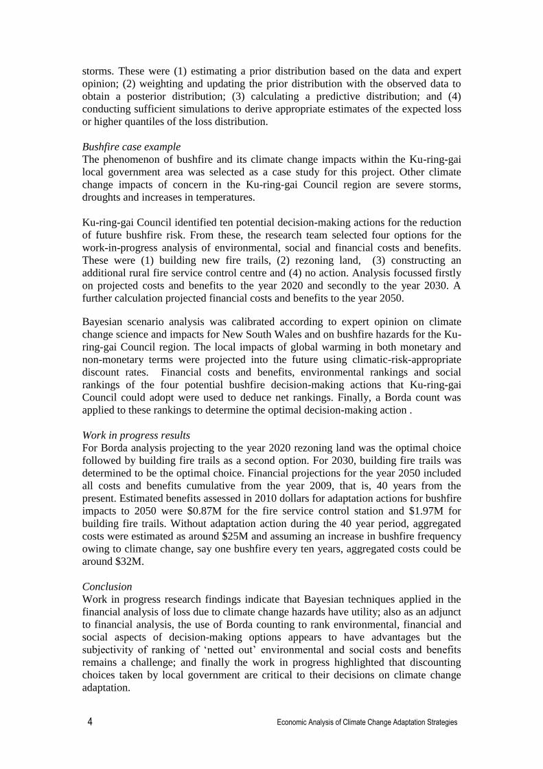
Bushfire case example
The phenomenon of bushfire and its climate change impacts within the Ku-ring-gai
local government area was selected as a case study for this project. Other climate
change impacts of concern in the Ku-ring-gai Council region are severe storms,
droughts and increases in temperatures.
Ku-ring-gai Council identified ten potential decision-making actions for the reduction
of future bushfire risk. From these, the research team selected four options for the
work-in-progress analysis of environmental, social and financial costs and benefits.
These were (1) building new fire trails, (2) rezoning land, (3) constructing an
additional rural fire service control centre and (4) no action. Analysis focussed firstly
on projected costs and benefits to the year 2020 and secondly to the year 2030. A
further calculation projected financial costs and benefits to the year 2050.
Bayesian scenario analysis was calibrated according to expert opinion on climate
change science and impacts for New South Wales and on bushfire hazards for the Ku-
ring-gai Council region. The local impacts of global warming in both monetary and
non-monetary terms were projected into the future using climatic-risk-appropriate
discount rates. Financial costs and benefits, environmental rankings and social
rankings of the four potential bushfire decision-making actions that Ku-ring-gai
Council could adopt were used to deduce net rankings. Finally, a Borda count was
applied to these rankings to determine the optimal decision-making action .
Work in progress results
For Borda analysis projecting to the year 2020 rezoning land was the optimal choice
followed by building fire trails as a second option. For 2030, building fire trails was
determined to be the optimal choice. Financial projections for the year 2050 included
all costs and benefits cumulative from the year 2009, that is, 40 years from the
present. Estimated benefits assessed in 2010 dollars for adaptation actions for bushfire
impacts to 2050 were $0.87M for the fire service control station and $1.97M for
building fire trails. Without adaptation action during the 40 year period, aggregated
costs were estimated as around $25M and assuming an increase in bushfire frequency
owing to climate change, say one bushfire every ten years, aggregated costs could be
around $32M.
Conclusion
Work in progress research findings indicate that Bayesian techniques applied in the
financial analysis of loss due to climate change hazards have utility; also as an adjunct
to financial analysis, the use of Borda counting to rank environmental, financial and
social aspects of decision-making options appears to have advantages but the
subjectivity of ranking of „netted out‟ environmental and social costs and benefits
remains a challenge; and finally the work in progress highlighted that discounting
choices taken by local government are critical to their decisions on climate change
adaptation.

Economic Analysis of Climate Change Adaptation Strategies
5
Future research recommendations
The techniques explored in this work in progress should be more widely applied than
for the Ku-ring-gai bushfire case study, i.e. in examination of further climate change
impacts for Ku-ring-gai Council and for other local government areas. Many local
government areas in Australia are subject to future bushfire risk; and as climate
change effects intensify, prioritisation information on local adaptation measures for
climate change issues related to drought, storms, flood damage and human health also
will be needed.
In future stages of the project, the research team envisages additional adaptation
issues for Ku-ring-gai Council will be addressed and ideally other local government
areas in Australia and overseas will be researched to give a more thorough
understanding of the applicability of the methods that have been examined in this
initial study.

Economic Analysis of Climate Change Adaptation Strategies
6
List of Abbreviations
ABC Australian Broadcasting Corporation
ARC Australian Research Council
BCA Benefit Cost Analysis
CBA Cost Benefit Analysis
CCAM Conformal Cubic Atmospheric Model
CRRA Constant Relative Risk Aversion
CFU Community Fire Unit
CSIRO Australian Commonwealth Scientific and Industrial Research
Organization
DCF Discounted Cash Flow
DDC Data Distribution Centre
DPV Discounted Present Value
EMA Emergency Management Australia
ENSO El Niño Southern Oscillation
ESD Ecologically Sustainable Development
ETS Emissions Trading Scheme
EU European Union / Expected Utility
EV Expected Value
FFDI Forest Fire Danger Index
GCM General Circulation Model
GCOS Global Climate Observing System
GHG Greenhouse Gas
GRI Global Reporting Initiative
IGBP International Geosphere-Biosphere Programme
IPCC Intergovernmental Panel on Climate Change
LDA Loss Distribution Approach
NSW New South Wales
NSWFB New South Wales Fire Brigade
OAGCM Ocean Atmosphere General Circulation Model
PDF Probability Density Function
PerilAUS Peril Australia (database)
QBL Quadruple Bottom Line
RCM Regional Climate Model
RFS Rural Fire Service
SES State Emergency Service
SRES Special Report on Emission Scenarios
TBL Triple Bottom Line
TGICA Task Group on Data and Scenario Support for Impact and
Climate Assessment
UN United Nations
UNFCCC United Nations Framework Convention on Climate Change
WCRP World Climate Research Programme

Economic Analysis of Climate Change Adaptation Strategies
7
1. Introduction
Greenhouse gas emissions are a global “bad”.
Garnaut 2008c, p. 173
1.1 Background and past related work
Ku-ring-gai Council, located on the North Shore of Sydney, may be particularly
vulnerable to increased storm and fire activity as predicted by climate change models
for the region (DECC 2008).The Council‟s vulnerability stems from its geographic
position in sharing boundaries with three National Parks, from its ridge top
development and from an extensive tree canopy. The Council has already recorded a
loss of $670 million from a single storm in 1991, and again in 1994 significant loss of
houses occurred owing to bushfire. The Ku-ring-gai Council local government area
(LGA) ranks third in bushfire vulnerability, defined as addresses within 130 metres of
bushland, among 61 LGAs in the Greater Sydney Region (Chen 2005).
Climate change mitigation and adaptation policy implementation have not been
handled on a comparable basis to date even though they are interrelated. Mitigation
efforts are aimed at reducing the likelihood of serious climate outcomes and are
focused on lessening the trajectory of atmospheric carbon dioxide concentrations.
Adaptation efforts are aimed at reducing the severity of any serious climate outcomes
that may be faced. As such, they are closely related, and decisions about the best
policy or mix of policies depends upon complex and sometimes contradictory factors
including: international treaties, for example the United Nations Framework
Convention on Climate Change (UNFCCC)‟s Kyoto Protocol which came into force
in 2005 and was ratified by Australia in December 2007; national legislation and
targets for example, the Carbon Pollution Reduction Scheme proposed for Australia
for 2010; regional requirements, for example the New South Wales (NSW) Climate
Change Action Plan; and local community desires and demands.
A literature review conducted as part of this study found no local government level
modelling explicitly linking mitigation and adaptation strategies and expenditures
although Council had previously undertaken assessment of potential local effects of
climate change which provided a foundation for the current analysis. In the absence of
directly relevant literature this collaborative effort would devise a tool generally
applicable to local government such that its methodology and therefore its outputs
would be consistent with social, environmental and financial assessment and the tool
itself would play a governance role, thereby completing the QBL reporting concept.
The prime objective of this project was to work towards developing a robust and
transferable tool to evaluate and prioritise greenhouse gas mitigation and climate
change adaptation strategies for local government decision-makers with Ku-ring-gai
Council as a collaborative partner. Four aims stemmed from this objective:
1. To identify and quantify actions and activities relevant to local government
that could support mitigation of greenhouse gas emissions and adaptation to
climate change.
2. To develop an economic model with appropriate discount rates to assess the
varying impacts within different climate change scenarios including costs and

Economic Analysis of Climate Change Adaptation Strategies
8
benefits to local government from action and inaction (not considering sea
level rise).
3. Using the model, prioritise strategies, policies and actions givenimmediate,
medium and long-term rankings for climate change impacts.
4. To assist decision-makers, incorporate the results into the Council‟s financial,
social, and environmental assessment framework.
1.1.1 Techniques
A. Economic modelling
The economic tool developed in this project uses a discounted cash flow (DCF)
modelling approach with Bayesian probabilities assigned by experts where data is
poor or unavailable. It is structured specifically to relate potential adaptation and
mitigation strategy expenditures to one another, so that direct comparisons may be
made where the strategies may be deemed substitutes (or mutually exclusive) and to
specifically account for the situations where they may be deemed complementary.
The DCF model demands that the appropriate discount rate or rates be employed to
enable comparison of present net value of benefits and costs of disparate cash-flow
patterns with net benefits and costs at specified future dates.
Determining the most appropriate discount rate is problematical since one must take
into consideration both the underlying cost of capital to support investment
expenditures for adaptive or mitigating projects and the relative riskiness of the flow
of future net benefits. Establishing the appropriate level of consideration that should
be given to intergenerational and intra-generational equity in regard to present
expenditure and future benefit is, in part, an ethical issue. Similarly the influence of
the uncertainty of the future on resulting net benefits and hence on the appropriate
discount rate is a point of discussion.
B. Regional downscaling
The political acceptance of the Intergovernmental Panel on Climate Change (IPCC)
Fourth Assessment (IPCC 2007) and economic reviews such as Stern (2006) and
Garnaut (2008a-c) seems to be driving exploitation of climate model simulations even
when inconsistent, and sometimes challenging, discrepancies are known, see for
example the Global Climate Observing System - World Climate Research Programme
– International Geosphere-Biosphere Programme Report, (WCRP 2008) and Doherty
et al. (2009). Today‟s challenge is how to select the tools most likely to be useful
from the plethora of model projections and proposed new analyses.
Local councils play a significant role in the management and protection of various
infrastructure and community assets. However there are limited tools available at the
local and regional level to assist in determining the most appropriate method of
adapting to and mitigating climate change. This limitation affects local governments
both nationally and internationally. Here, the climate projection skills of models
involved in the IPCC Fourth Assessment Report are exploited for regional
downscaling to the extent that this can be shown to be viable. Specifically we draw
on the extensive analysis reported by the NSW Department of Environment and
Climate Change (NSW 2008a)

Economic Analysis of Climate Change Adaptation Strategies
9
C. Comparing monetary and non-monetary values: Triple Bottom Line (TBL)
assessment
Ku-ring-gai Council has introduced a performance reporting process that is framed by
environment, society, economy and governance (QBL). For the purposes of
examining options, only the first three, referred to as Triple Bottom Line (TBL), are
required. Governance relates to the manner in which the Council deals with the
information once obtained and therefore does not directly apply to the analysis of
options. The inclusion of governance in the framework is consistent with the
requirement of the Global Reporting Initiative (GRI 2007) which is the preferred
sustainability framework endorsed by the NSW Government in 2007 and used by Ku-
ring-gai. Such a framework enables direct and indirect performance of the Council to
be analysed from individual employee work plans through to long term strategic
Council policies.
The prioritisation tool developed here relates market, or financial costs and benefits to
non-market environmental and social assessments in a Triple Bottom Line context.
The tool itself plays the role of governance in providing a mechanism for policy and
operational decision-making.
1.2 Literature review emphases
A literature search for „economic analyses since 2003 of the economic costs of
mitigation and adaptation to climate change at the local government level‟ reveals
much world-wide interest in the subject, accompanied nevertheless by a lack of
modelling at the local level. Impacts of climatic change have been studied extensively
by the natural sciences, but research on the social and economic consequences is more
limited (Kuik et al.2006).
Kuik et al.(2006) also note that insufficient work has been done on the costs of
adaptation versus no adaptation as well as on what changes there might be to
adaptation costs if there were some level of mitigation. The importance of such work
re-emerges in Garnaut‟s (2008a) conclusion where he implies that the high costs of
climate change do not in themselves make a case for any level of mitigation, rather a
comparison of the costs of mitigation must be weighed against the costs saved from
avoided climate change. He later states „Both the costs and benefits of mitigation, but
especially the benefits, reveal themselves over much longer time frames than
humanity is accustomed to taking into account (Garnaut 2008b p24).
Agrawala et al. (2008) note that the literature concerning mitigation is comprehensive
and demonstrates clear boundaries to the concept of mitigation, while the literature for
adaptation remains sparse and contested and without clear boundaries or a metric for
assessing the effectiveness of adaptation measures. Nevertheless, governments at
local and national levels will implement adaptation action because of its public-good
characteristics. Studies at the local level have been restricted to certain sectors such as
public health and tourism. Also, there has been very little attention to governments‟
role in facilitating private adaptation investment decisions.
The following section examines progress with economic modelling and management
toolsfor climate change reported in the recent literature, then summarises methods for

Economic Analysis of Climate Change Adaptation Strategies
10
valuing non-market goods, next considers the controversial topic of discount rates,
then briefly refers to downscaling, and finally looks at the important topic of
behavioural and psychological aspects of adaptation.

Economic Analysis of Climate Change Adaptation Strategies
11
2. Relevance of Current Climate Change Economic Analysis to Local
Government Decision-Making
Some aspects of climate change economic analyses to date have utility in assisting
those involved in the challenging area of climate change decision-making at the local
government level. Academic views on climate change economic approaches, methods
for valuing non-market goods, discount rates, downscaling, and behavioural and
psychological aspects of adaptation are covered in this section.
2.1 Climate change economic approaches
Economic approaches to climate change range in scale and method from integrated
climate and economic models to Benefit Cost Analysis. Selected approaches reported
in the literature are described below:
1. Integrated models
2. Risk models including Adaptive Monte Carlo optimisation
3. General equilibrium models
4. Integration of mitigation and adaptation measures
5. Urban impacts and adaptation strategies
6. Transient impact and adaptation modelling
7. Benefit Cost Analysis (BCA) applied to disaster mitigation
8. Fuzzy logic
2.1.1 Integrated Models
Many researchers advocate an integrated approach or an integrated modelling
approach to linking climate change science, impacts and socio-economic factors for
decision-makers although the term integrated is used with a variety of meanings.
Among those advocating integration in one form or another are Ermolieva and
Sergienko (2008), Jones et al.(2007), Kirshen et al. (2008), Kuik et al. (2006) and
Godard (2008). Kuik et al.(2006) distinguish integrated approaches from exogenous,
or externally influenced approaches. Also Godard (2008) observes that integrated
assessment models are intended to capture interactions between natural and economic
systems and the aim should be „projected equilibrium‟ where achievements match
expectations and should include generational equity. However, fully dynamic
integrated approaches, linking long-term socio-economic feedback and climate
scenarios to the costs of inaction, are rare.
2.1.2 Risk insurance theory, application to floods, Adaptive Monte Carlo optimisation
Ermolieva and Sergienko (2008) review models and approaches taken in managing
catastrophic risk. Planning for natural risks requires a strict risk-specific
methodology. They acknowledge that mathematical models for quantitative
assessment and prediction that can deal with incomplete information are necessary.
The fact that a one-in-500 years event may occur tomorrow is all too often overlooked
by traditional deterministic models.
They also point out that catastrophes have the characteristic of being infrequent in any
given locality; they may not resemble one another, meaning that past experience is not

Economic Analysis of Climate Change Adaptation Strategies
12
a reliable guide; and there are few or no real observations to facilitate traditional
statistical modelling based on the law of averages. Furthermore, claims and losses for
particular insurance categories cannot be assumed to be independent of one another as
are vehicle and household claims.
Ermolieva and Sergienko (2008) show that stochastic optimisation models are useful
and they provide a version of the Adaptive Monte Carlo optimisation approach (see
Section 4.6.2 The Loss Distribution Approach). They refer to a „three-dimensional‟
model of catastrophic flooding which was developed to create artificial data with
which to supplement incomplete data on past floods, possible damage, dependence on
different management strategies; and to make projections. This integrated risk control
model allows for evaluating risk reduction actions and consists of three moduli:
1. possible increase of river levels
2. the vulnerability of individual buildings at various inundation levels and
3. a stochastic model of economic growth which relates income loss to local and
central governments, households, the catastrophe fund, insurance companies,
investors, and producers.
The authors conclude that stochastic optimisation models are valuable in taking into
account the goals and constraints of the different agents, and that an integrated
approach including preventive measures to reduce catastrophe probabilities is
necessary. The Ermolieva and Sergienko (2008) method may be useful as central
governments shift responsibility and cost to local government agencies and actors.
2.1.3 General equilibrium model
Calzadilla et al.(2005) use a dynamic computable general equilibrium model to assess
the impact of climate change on El Niño Southern-Oscillation and the North Atlantic
Oscillation cycles and expected losses at the regional level. The authors note that
local impacts of economic loss propagate within the globalised world economy. They
remark, however, that although climate scientists are studying these relationships, no
model is available that links climate change to local extreme weather conditions.
Their paper does not address climate change adaptation or mitigation efforts.
Kuik et al. (2006) use the term general equilibrium effect to refer to the economy as a
whole. Indirect effects of climate change, having been spread throughout the
economy by the markets, can amplify and diminish the direct economic impacts of
climate change. Most studies to date have underestimated the indirect economic
effects on the general economic equilibrium.
2.1.4 Integrating mitigation and adaptation measures: management level
Jones et al. (2007) explore the critical complementarity of mitigation and adaptation
and the need for an integrated approach by managers. They describe the case of two
Australian regional bodies, the Central Victorian Greenhouse Alliance and the North
Central Catchment Management Authority, that maximise the benefits of mitigation
and adaptation actions through integrating such actions at the regional scale.
They believe that Australian policy affecting adaptation and mitigation is likely to be
„top down‟ from the state or national level, while the actors are local. Central and
state governments may favour large, visible projects such as large power generator

Economic Analysis of Climate Change Adaptation Strategies
13
initiatives or large industrial processes, yet in Northern Victoria it appears smaller
niche generators using renewable energy sources and cogeneration may be well
placed to provide power.
The bodies both recognise that regional reductions in greenhouse gases will not
directly benefit the local area but rather will contribute to the global common good.
However, they do believe that a local area being an early adopter of mitigative
technologies and actions will provide economic benefits. White et al. (2008) share
this optimism in considering policy options for English Regional Development
Agencies and local authorities who seek opportunities for business and the economy
as a whole while responding to the government‟s carbon reduction pathway
obligations.
2.1.5 Case study of integrated urban impacts and adaptation strategies
Somewhat resembling Sydney, Boston‟s population is 3.2 million, increasing to 4
million by 2050 (Kirshen et al.2008) its boundaries comprise a harbour fed by three
rivers and a ring road; its population density is concentrated in the east, spreading out
generally westward to suburbs and then to farmland and some urban „sprawl‟.
Serving as an air and sea gateway to the northeast of the United States, Boston‟s
infrastructure is ageing (Kirshen et al.2008)
Although Kirshen et al. (2008) analyse Boston‟s urban infrastructure systems in the
northeast of the United States, they recognise, similarly to Jones et al.(2007), the
interdependencies of climate change impacts and adaptation actions.
The article summarises the implications regarding energy use, coastal and river
flooding, transport, water supply and quality, public health, tall buildings, and bridge
scouring infrastructure systems. The authors observe:
1. Structural actions taken before full climate change impacts occur will result in
fewer total expected negative impacts
2. Actions taken soon will result in less negative weather related impact even
without climate change
3. Climate change will magnify negative impacts due to demographic changes
4. Climate change impacts and largely complementary adaptations will not only
affect target infrastructure systems but also interrelated systems, and
5. Adaptation actions must be integrated with land use planning, environmental
impact assessments, and socio-economic impact assessments, for example, of
disrupted supply chains.
2.1.6 Transient impact and adaptation model
Hallegatte‟s (2005) integrated global model takes into account the inertia of climate
and socio-economic systems. The author finds that the climate-economy feedback
takes 50 to 100 years and cannot act as a damper on climate change; results of
emission reductions appear after 20 years; results are better seen in 50 years; and
mitigation efforts are significant over more than one century. Emissions linked to
economic growth create additional climate change damage, and hence a cost to the
climate from growth.

Economic Analysis of Climate Change Adaptation Strategies
14
2.1.7 BCA/CBA applied to disaster mitigation
Ganderton (2005) asserts that Benefit-Cost Analysis (BCA) / Cost Benefit Analysis
(CBA) is the most appropriate method for assessing hazard mitigation actions as it
takes into account all the benefits that may be achieved by a mitigation action. He
warns against keeping benefits constant as with Cost Effectiveness Analysis, where
benefits, often non-monetary, are stated and fixed at a particular level thereby
ignoring other non-specified benefits that result from the action. He comments that
although projects should be evaluated from society‟s point of view, decision makers
often have to confine themselves to one sector or level of government. They must also
recognise that not all people see an action as a benefit; some may see it as a cost.
Analysts must deal with the counterfactual: if hazard mitigation does not take place,
it may depress economic activity or other activity in the affected area. Unfortunately
BCA has not produced a definitive prescription for dealing with uncertainty, a major
issue in anticipating risk induced by climate change (Ganderton 2005).
However, Norman et al. (2007) doubt that CBA is the appropriate tool for analysis of
global problems that extend over centuries and impact non-human species(see Section
4.3 Climate predictions). They find that ex-ante estimations of costs may be higher
than later, realised ex-post estimations, owing to research breakthroughs that lowered
cost or improved quality.
2.1.8 Fuzzy set operations
Prato (2008) shows how fuzzy set logic can be applied when there is uncertainty
about the nature and extent of climate change impacts. Where set membership is
vague, ambiguous or nonexclusive, fuzzy logic, particularly the operation known as x-
cuts, is useful for defining climate change variables and their impacts on a managed
ecosystem. Prato (2008) considers the cases where subjective probabilities of climate
change scenario are assigned, preferably by experts, and where probabilities cannot be
assigned. Bayes rule or Bayesian techniques (Lee 2004) can be used to update
assigned probabilities as more data become available (see Section 4.7).
2.2 Valuing non-market goods
Economists employ various methods for assigning monetary values to non-market
goods such as environmental values. Ganderton (2005) describes revealed preference
methods, where behaviour is actually observed, such as Value of Intermediate Goods,
Hedonic Price Models and Travel Cost Models. He also describes stated, or
hypothetical, preference models such as the Contingent Valuation Method and
Conjoint Analysis. The Benefits Transfer Method uses existing data from other
projects and can be less expensive. Rehdanz (2007) uses spatial econometric
techniques to value ecosystems. Kuik et al. (2006) believe that although all current
studies use a mix of valuation techniques, a rough version of Benefit Transfer is the
predominant method used. Unfortunately studies into the effects of one valuation
method over another are lacking.
Ganderton (2005) reminds us that environmental economists find that the wider
society places very high values on the existence of ecosystems; furthermore

Economic Analysis of Climate Change Adaptation Strategies
15
economists cannot measure the emotional and psychological dimensions of disaster
mitigation.
Rehdanz (2007) investigates how European Union (EU) citizens value species
preservation, biodiversity and ecosystem services. Humans place value on the
proximity of ecosystems that conserve biodiversity and reduce numbers of threatened
species. The author links human life-satisfaction with biodiversity and numbers of
threatened species by using spatial econometric techniques to determine whether
spatial relationships exist and to what extent. A mammal species was shown to be
valued more than a bird species; however overall bird species seem to be a better
indicator of biodiversity.
Kuik et al. (2006) prepared a table (Table 2.1) showing the key methodological issues
that they identified wereassociated with nine selected climate change cost studies
from 2001-2006. Issues needing further research highlighted by Kuik et al. were
valuation of non-market goods, adaptation costs and uncertainty.
Table 2.1.Key methodological issues identified with nine selected climate change
cost studies (Kuik et al. 2006, p. 15)
2.3 Discount rate
Karp (2005) advises the discount rate chosen may ultimately determine the cost-
benefit ratio for investments related to climate change. Even moderate discounting
discourages small present-day investments to avoid large damages in the distant
future.

Economic Analysis of Climate Change Adaptation Strategies
16
Summers and Zeckhauser (2008) take the view that market rates of discount are too
high for projects benefiting society as a whole, and that social investments should
give the future far more weight than do private projects. Humans, particularly those
alive today, have despoiled the environment, and future generations have as much
right to inherit a hospitable earth as we did. They point out that humans are shown to
have a strong aversion to causing suffering or loss, and their valuing of non-monetary
goods rises disproportionately with rising income; while standard discounting implies
that an increment in consumption will have less marginal utility among richer future
generations. The fact that there will be more people should accord the future a
proportionately greater weight than calculations ignoring population increase.
Furthermore, we are able to learn from actions taken now. The authors present the
examples of Thomas Edison‟s inventions, the Internet, and technology developed for
the armed forces in World War II – all of which progressed human welfare into the
21st century and presumably beyond. Knowledge gained from actions taken now is
not appropriable.
Summers and Zeckhauser (2008) propose a „4D‟ mnemonic:
Discounting – the future deserves a high value
Disaster – climate change will impose a very high cost at some future date
Distinction – society makes a distinction between types of investment for the
future
Decision analysis – the greater the uncertainty, the greater is the danger in
waiting. The cost of action is increasing at an increasing rate; and, learning
from actions taken now could reduce the overall cost of optimal efforts.
Kuik et al. (2006) observe that very few studies incorporate a measure of statistical
risk. There is uncertainty regarding future discount rates; in fact there is no agreement
in the empirical literature as to how a discount rate should be chosen. In their
overview of the literature they present the following viewpoints on discounting:
Discounting is equivalent to the present generation owning all future
resources. Although objectionable from a moral standpoint, it seems to reflect
current reality. This line of research has not led to practical alternatives to
discounting. A constant rate of pure time preference between 1 and 3 percent
is employed by most studies.
Conventional exponential discounting accords the same difference between
two years whether they fall in the present decade or in a century from
now. That is, using the discount factor (1+r)-t, where r = the rate of discount
and t = time, leads to that effect.
Hyperbolic discounting could be implemented with one year in the present is
equivalent to ten years in one hundred years’ time. Present discount rates
would be little affected and would mainly affect long-term decisions.
A low discount rate puts the cost of inaction with regard to the environment
and climate change much higher than does a high discount rate.
A hyperbolic discount rate (becoming lower over time) assigns higher
marginal damage costs as the discount declines.

Economic Analysis of Climate Change Adaptation Strategies
17
Other commentators on discount rates in association with future generations and
climate adaptation include Garnaut (2008c), Karp (2005), Kirshen et al. (2008),
Ganderton (2005), Ismail-Zadeh and Takeuchi (2007) and Winkler (2006). Garnaut‟s
Final Report (2008c) provides a discussion of the effects of different discount rates as
it relates to climate change adaptation. Karp (2005) affirms other researchers‟ views
that hyperbolic discounting tends to conform with psychological perceptions of value
over time and reduces the problems associated with constant discounting.Kirshen et
al. (2008) avoid the ethical arguments surrounding the discount rate by not
discounting any impacts of climate change, thereby assuming that property values and
adaptation costs appreciate at the same rate.Ganderton (2005) notes that in a Cost
Benefit Analysis, the scope of a mitigation project involves both spatial and temporal
aspects. If a project has intergenerational impacts, then future generations should
receive standing in any project that impinges upon them.Ismail-Zadeh and Takeuchi
(2007) find the standard discount rate approach inadequate for making decisions
about when to take preventative measures in relation to extreme natural events such as
the numerous earthquakes, tsunamis, floods, and cyclones that have already occurred
in the 21st century.On the other hand, Winkler‟s (2006) analysis finds that the
outcome of hyperbolic discounting is not only unsatisfactory from the present
generation‟s point of view, but may also be inefficient. This is because hyperbolic
discounting assumes that the present generation faces the costs of investment while
the benefits are spread over all subsequent generations. Winkler (2006) challenges
the use of hyperbolic discounting in long-term decision making. Success in
hyperbolic discounting requires a commitment mechanism.
For further discussion on discounting including Cost Benefit Analysis, see Section
4.4Choosing a discount rate: how are non-market values included?
2.4 Downscaling
Kirshen et al. (2008) looked at present climate projected without change as well as at
two climate change scenarios; they used three different climate change adaptation
scenarios; and they used only one set of population projections in order to emphasise
adaptation and climate sensitivities. The researchers used climate change scenarios
developed for the American New England region, and obtained scenario data for the
inland grid cell closest to the study area for 2030 and 2100. They assumed that the
downscaled results did not differ significantly from more coastal grid cells.
In an editorial review article, Frumhoff et al. (2008) describe the work of Hayhoe et
al. (2008) in the same issue. The results of three global circulation models are
downscaled to regional northeast United States. The average of the downscaled
model outputs reproduces temperature and precipitation trends across the northeast of
the United States except for recent winter warming, possibly owing to small-scale but
important feedback effects of reduced surface snow cover.
For a discussion of regional downscaling, see Section 4.1 Climate change
downscaling, and for a summary of downscaled, projected impacts see Section 4.2
Climate change overview.

Economic Analysis of Climate Change Adaptation Strategies
18
2.5 Psychological and behavioural aspects
Agrawala et al. (2008) believe that although there are sectors like agriculture and
some behaviours such as reducing water consumption where a high benefit/cost ratio
will assist in making adaptation decisions, the relative ease of costing infrastructural
adaptations over behavioural efforts may lead to a bias toward the „hard‟ adaptation
measures as well as overestimating adaptation costs. Furthermore, successive studies
tend to build upon the assumptions made in previous studies, and therefore cannot be
considered truly independent.
Byrne et al. (2007) and Ismail-Zadeh and Takeuchi (2007) find that although citizens
and regional, state, and local governments in the US want policies that address
climate change mitigation, and to a lesser extent adaptation (such as „weatherising‟
low income housing), the Federal Government procrastinates and has even been seen
to impede efforts.
Knetsch (2007) asserts that it makes a difference which valuation method for
environmental damage is chosen as the choice can bias outcomes. People value loss,
or the avoidance of loss, more highly than equivalent gains. In cost-benefit analyses,
the „willingness to pay‟ method results in a lower valuation than the „willingness to
accept‟ method. The implication is that people will put a higher present value on a
future loss than on the expectation of a future gain. People discount future gains more
than future losses. Different discount rates should be used for future loss and future
gain, and this would likely accord more weight to future environmental loss.
Gardner and Stern (2008) provide a number of energy retrofit options for homes.
They find that although financial incentives are indeed a motivating factor, public
information campaigns and government commitment to facilitating the energy-saving
actions are by far the most effective at invoking householder investment.
2.6 Conclusions
There have been surprisingly few studies at the local level on the economic cost of
mitigation and adaptation in relation to climate change impacts. Studies that do exist
have tended to focus on particular economic sectors such as agriculture, tourism and
health.
Global climate models provide scientific information, but current integrated models
do not adequately integrate socio-economic feedback from mitigation and adaptation
efforts. Integrated approaches being more recent are important for incorporating the
effects of human socio-economic attempts to deal with climate change. Uncertainty
characterises the discussion; the term „equilibrium‟ can be applied to geophysical
climate scenarios as well as to modelled socio-economic dynamics. Likewise the term
„integration‟ has various applications including complementary impacts on
infrastructure, but seems usually to apply to feedback between geophysical and socio-
economic forces.
With regard to risk modelling, the fact that a one-in-500 year event could occur
tomorrow is often overlooked by traditional deterministic models and confounds the

Economic Analysis of Climate Change Adaptation Strategies
19
basis of risk insurance theory. There is a body of literature dealing with preparedness
for such events.
Also there has been insufficient study into the costs of the „reference case‟ of no
adaptation effort. Mitigation studies exhibit defined boundaries, while adaptationas a
concept arguably remains amorphous.
Assigning costs and benefits to present-versus-future-generations in the face of
uncertainty enmeshes ethical, and therefore controversial, considerations. No
satisfactory method for assigning dollar values to non-market environmental services
exists despite human attempts to approximate a value for what is essentially priceless.
Because of their public-good characteristics, mitigation and adaptation efforts must be
guided by government.Not enough effort has been invested in facilitating private
expenditure both business and residential. Accordingly, local government may find
that its greatest value-for-dollar climate adaptation efforts lie in encouraging private
households to invest in adaptation. In taking this path it may address the
psychological and behavioural aspects of adaptation by reducing restrictions, for
example, on solar panels and water tanks, and providing market information such that
each household need not do its own extensive research into sustainable renovation
options. Such action, however, may be yet another extension of local governments‟
responsibilities into the domain of the state owned utilities and corporations.

Economic Analysis of Climate Change Adaptation Strategies
20
3. Climate Change Implications for Local Government
Climate change mitigation and adaptation is challenging and requires input from all
levels of government. At the local level where action is often the most effective, local
government confronts the complex and problematic task of planning and
implementing mitigation and adaptation actions within existing budgetary, legislative
and policy constraints. While the NSW State Government has provided funding for
some initial climate mitigation and adaptation initiatives such as energy and water
savings, the effects of altered weather patterns associated with a changing climate are
generating a plethora of inter-connected impacts that demand a sophisticated multi-
disciplinary, multi-faceted response.
3.1 Bushfire risk as the focus of the present study
Planning short, medium and long term responses to climate change at the local level
will build on existing knowledge of historical risks. While climate change may
impose new risks in some local jurisdictions, for Ku-ring-gai the modelling suggests
that no new risks are likely to emerge, however existing weather related risks are
likely to intensify. The challenge is to ascertain the significance of the predicted
effects of climate change and to identify local consequences in relation to future
liability. Decision-makers must also consider the benefits foregone and the cost of
failure to take pre-emptive action to mitigate and adapt to the more extreme impacts
of climate change. Planning for climate change has the potential to involve many
broad areas of responsibility for the local government sector including, but not
restricted to:
Bushfires frequency and intensity
Storms frequency and intensity
Water security as related to potable supply per capita
Biodiversity such as the loss of Critically Endangered Vegetation
communities, and
Heat stress mortality rates
The above areas of concern were identified through a community consultation process
undertaken by Ku-ring-gai Council. From this list, the Council and the researchers
selected intensified bushfire risk as their focus for this study.
Planning responses to increases in bushfire risks are complex and fall within the
auspices of a number of public agencies and private land managers. Ku-ring-gai
Council has responsibility for proactively managing bushfire risk along its 89-
kilometre urban-bushland interface along with other land managers through joint
management agreements. These areas are subject to periodic high intensity fire
activity and consequently the community is highly vulnerable to this threat. Fire
events causing loss of property between 1997 and 2007 occurred in the years 1977,
1980, 1991, 1992, 1994, 2002 and 2004.
Although loss of life owing to bushfire is rare in this region, house losses are not. The
economic and social impacts of bushfire events are well documented while
environmental impacts are less well understood. Environmental impacts may not be

Economic Analysis of Climate Change Adaptation Strategies
21
immediate but can emerge over time as intensity and frequency of fires increases. For
example, erosion, a function of soil type, slope, vegetation cover and rainfall
intensity, occurs for a period of time after fire, particularly on the steep slopes and
sandstone soils found in Ku-ring-gai. Hot weather in Sydney is often terminated by a
southerly change accompanied by thunderstorms and heavy rain. This combination of
weather patterns leads to an accelerated process of erosion which degrades slopes and
deposits sediments in local creeks and waterways choking the biological life of those
assets.
The frequency of major fires is exacerbated by arson. The intensity of fires is
influenced by fuel characteristics such as mass, structure, moisture levels and type of
weather conditions including wind speed, humidity, cloud cover, atmospheric stability
and temperature (UTS 2004, pp. 3-5). Ku-ring-gai vegetation communities contain
highly combustible forest types located ina topography of deeply incised valleys
crowned by ridge top urban development. Slope has a direct effect on the rate of fire
spread and behaviour. Assuming a constant fuel load, for every 10 degree increase in
slope, the rate of spread of fire doubles (UTS 2004, p. 6). Aspect also plays a role;
north facing slopes are exposed to greater solar radiation and thus support drier fuels.
This means that the north and northwest facing slopes which occur in up to half of
Ku-ring-gai‟s urban-bushland interface will on average burn more often and over a
larger number of days, including days not classified as extreme bushfire weather
(UTS 2004, p. 6).
3.2 Planning for bushfire protection in Ku-ring-gai
„Planning for Bushfire Protection‟ (NSW Rural Fire Service 2006) sets out key
strategies for minimising bushfire risk in NSW. Protection of life and property is the
primary objective of this plan particularly in relation to planning new developments.
The Rural Fire Service (RFS) has the responsibility to review development
applications and considers their merit from the point of view of bushfire protection.
These measures are designed to ensure the risk to new homes and residents from
bushfire is minimised.
However, prior to this guideline and the introduction of the Rural Fires Act
1997(NSW), development within areas prone to bushfire did not have to consider
bushfire risk. Consequently urban planning and constructed prior to 1997 had
considerable latitude in the interpretation of risk; and while councils could require that
bushfire protection measures be incorporated into the development they could do little
to stop development in bushfire prone areas. As a result, thousands of homes across
the Ku-ring-gai local government area are located at the bushland interface and are
vulnerable to fire risk. Figure 3.1 shows the extent of the high risk areas which nearly
encircle the local government area.
Commentary by the Insurance Council of Australia in February 2009 in the aftermath
of the devastating Victorian fires suggests that building codes in Australia fall well
below international standards. The Insurance Council believe this anomaly combined
with homes facing the consequences of more severe weather conditions will likely
mean that home owners will find it increasingly expensive and difficult to insure
(SMH 5 February 2009, p3).

Economic Analysis of Climate Change Adaptation Strategies
22
Figure 3.1. Ku-ring-gai Local Government Area: high bushfire risk areas (Source:
Ku-ring-gai Council)
3.3 Fire vulnerability
The physical setting and development pattern across the Ku-ring-gai local government
area creates a number of risk factors when considering the vulnerability of natural and
built assets to bushfire. These include:
18,000 hectares of bushland
89 kilometres of urban / bushland interface
13,000 or 36 per cent of houses with a high fire risk rating.
For these reasons, the local government areas has been ranked as third in bushfire
vulnerability of the 61 local government areas in the Greater Sydney Metropolitan
Region (Chen 2005).
Recognising this risk, Ku-ring-gai Council has implemented a range of planning,
operational and community strategies to reduce bushfire vulnerability. Access and
egress are recognised as significant issues in some localities that have lead to
restrictions for certain development types. This is in addition to mapping of bushfire
prone areas (RFS 2006). Notwithstanding these recent planning and development

Economic Analysis of Climate Change Adaptation Strategies
23
restrictions there are many schools, aged care facilities, hospitals and recreational
facilities that are considered highly vulnerable, particularly in relation to evacuation.
Investment in bushfire risk reduction strategies has been a key focus of Ku-ring-gai
Council over the past ten years. Figure 3.2 shows Council investment by functional
area in the 2006-2007 financial year. The success of these strategies in reducing risk
is difficult to quantify and in many cases will only be realised during and following a
bushfire event.
Figure 3.2. Ku-ring-gai Council expenditure on bushfire protection 2006-2007
3.4 Fire and emergency services roles in bushfire
The NSW Fire Brigade (NSWFB) is the lead agency for structural fires. However it
has a role in other fire types including bushfires. The focus of the NSWFB is mainly
urban while the Rural Fire Service (RFS) concentrates on peri-urban and rural areas.
The NSWFB promotes and trains Community Fire Units (CFUs) to act until fire
services can arrive. CFUs are volunteer groups that receive training and equipment to
prepare and protect their property and neighbouring properties from spot fires and
ember attack when bushfires threaten. A typical Community Fire Unit consists of 6 to
12 local residents who live on the same street, although family and friends living
within a 2-kilometre radius are able to join particular CFUs (NSW FB 2009). The
State Emergency Service (SES) also plays a role in fire events. In addition to its
primary role of emergency and rescue services, the SES assists other emergency
services during major operations. These services include the NSW Police Force, the
NSW Rural Fire Service, NSW Fire Brigades and the Ambulance Service of NSW.
The Ku-ring-gai community can rely on all these agencies in the event of storm, fire
or other emergency. Ku-ring-gai Council provides financial assistance to these
agencies and contributes to their annual running costs (see Figure 3.2).
Economic Analysis of Climate Change Adaptation Strategies
24
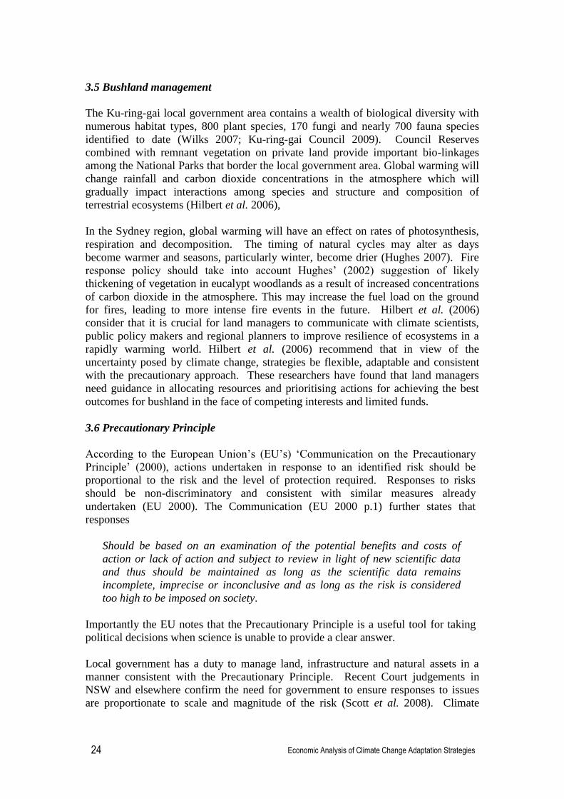
3.5 Bushland management
The Ku-ring-gai local government area contains a wealth of biological diversity with
numerous habitat types, 800 plant species, 170 fungi and nearly 700 fauna species
identified to date (Wilks 2007; Ku-ring-gai Council 2009). Council Reserves
combined with remnant vegetation on private land provide important bio-linkages
among the National Parks that border the local government area. Global warming will
change rainfall and carbon dioxide concentrations in the atmosphere which will
gradually impact interactions among species and structure and composition of
terrestrial ecosystems (Hilbert et al. 2006),
In the Sydney region, global warming will have an effect on rates of photosynthesis,
respiration and decomposition. The timing of natural cycles may alter as days
become warmer and seasons, particularly winter, become drier (Hughes 2007). Fire
response policy should take into account Hughes‟ (2002) suggestion of likely
thickening of vegetation in eucalypt woodlands as a result of increased concentrations
of carbon dioxide in the atmosphere. This may increase the fuel load on the ground
for fires, leading to more intense fire events in the future. Hilbert et al. (2006)
consider that it is crucial for land managers to communicate with climate scientists,
public policy makers and regional planners to improve resilience of ecosystems in a
rapidly warming world. Hilbert et al. (2006) recommend that in view of the
uncertainty posed by climate change, strategies be flexible, adaptable and consistent
with the precautionary approach. These researchers have found that land managers
need guidance in allocating resources and prioritising actions for achieving the best
outcomes for bushland in the face of competing interests and limited funds.
3.6 Precautionary Principle
According to the European Union‟s (EU‟s) „Communication on the Precautionary
Principle‟ (2000), actions undertaken in response to an identified risk should be
proportional to the risk and the level of protection required. Responses to risks
should be non-discriminatory and consistent with similar measures already
undertaken (EU 2000). The Communication (EU 2000 p.1) further states that
responses
Should be based on an examination of the potential benefits and costs of
action or lack of action and subject to review in light of new scientific data
and thus should be maintained as long as the scientific data remains
incomplete, imprecise or inconclusive and as long as the risk is considered
too high to be imposed on society.
Importantly the EU notes that the Precautionary Principle is a useful tool for taking
political decisions when science is unable to provide a clear answer.
Local government has a duty to manage land, infrastructure and natural assets in a
manner consistent with the Precautionary Principle. Recent Court judgements in
NSW and elsewhere confirm the need for government to ensure responses to issues
are proportionate to scale and magnitude of the risk (Scott et al. 2008). Climate

Economic Analysis of Climate Change Adaptation Strategies
25
change modelling predicts future climate shifts at regional levels but there remains
uncertainty at the local scale which creates dilemmas for councils.
Guided by the Local Government Act1993 (NSW), Ku-ring-gai Council has
determined that strategic planning should be consistent with the Principles of
Ecologically Sustainable Development (ESD). The Council has adopted a Quadruple
Bottom Line reporting framework to integrate existing management and reporting
systems. A benefit-cost framework guided by ESD Principles has been explored to
enable a more accurate system of identification of transparent, community referenced
priority areas for investment in long-term climate change mitigation and adaptation
policy.
The Precautionary Principle guides decision-makers in areas of complexity where no
clearly defined answers exist to risks with serious or irreversible consequences (Local
Government Amendment (ESD) Act, 1997). Uncertainty characterises decision-
making where environmental change is concerned. Pindyck (2007) notes we cannot
know with much precision the effects created by environmental damage even though
we may spend considerable resources trying to find out. In regard to climate change,
Pindyck claims that the very long time horizons and the ability of humans to adapt
make it very difficult to pinpoint the impacts. Pindyck (2007 p.29) claims that there
will inevitably be hidden or unanticipated costs and benefits that emerge as a result of
policy change due to the dynamism and complexity of climate change scenarios and
their associated uncertainties.
Given the transitional nature of legislation and public perceptions relating to climate
change, it would be prudent of councils to adopt both adaptation and mitigation
measures that address the risks posed by climate change.
3.7 Legal framework
In planning for climate change, it is worth noting the growing number of successful
administrative challenges involving climate change in the NSW Land & Environment
Court and other jurisdictions around Australia (NSW LEC, 2006). The NSW Land &
Environment Court has jurisdiction over local government matters and appears to be
receptive to the consideration of future climate change. The outcomes of these cases
have hinged upon the application of the ESD Principles as defined in the
Environmental Planning and Assessment Act 1979 (NSW):
the Precautionary Principle
inter-generational equity
conservation of biodiversity and ecological integrity
improved valuation, pricing and incentive mechanisms.
As these Principles also appear in the Local Government Act1993 (NSW), it is clear
that local government must have regard to them in managing the environment.
Litigation regarding climate change issues may occur via the common law of tort.
While the likelihood of successful litigation appears low due to difficulty in proving
specific causation, this may change as McDonald (2007, p. 407) notes:

Economic Analysis of Climate Change Adaptation Strategies
26
Like the tail-effect of greenhouse gas emissions, legal claims may be
slow to gestate. But the law has a long memory, so courts of the future
will reflect on the state of knowledge currently at hand to determine
whether decision-makers of today did enough to avoid or minimise the
worst exposures to climate change.
The need for due diligence on behalf of local government is outlined by England
(2007, p. 14):
Local governments currently have available to them a number of
defences that seem likely to protect them from claims based on a failure
to recognise and respond to information about climate change.
Nevertheless, just as the science of climate change is gathering
momentum, so too the law in this area is evolving rapidly. Local
governments should therefore take care to ensure their actions,
decisions and policy responses to matters that may either contribute to,
or be affected by, climate change remain current and reasonable in
what is a rapidly evolving policy context.
Several factors must be taken into account when considering whether a duty of care
exists giving rise to negligence, including:
available knowledge,
the degree of control,
specificity and
vulnerability of the claimant arguing the existence of the duty.
(Perre v Apand (1999); Sullivan v Moody (2001); Graham Barclay Oysters Pty Ltd v
Ryan; Ryan v Great Lakes Council; New South Wales v Ryan (2002))
Local government may be seen to have considerable control over developments for
which it is the consent authority (McDonald 2007) and as a result local authorities
may be considered easier targets for litigators. Establishing a causal connection
between a development approval in an area vulnerable to future climate change
impacts and subsequent property damage is more readily proved than damage arising
from the actions of one particular greenhouse emitter (McDonald 2007, p. 407).
However the Civil Liability Act2002 (NSW) provides local authorities with some
protection from being held negligent. A local authority will only be held liable for an
act or omission where it has acted unreasonably, and this will be determined with
reference to the limitations on financial and other resources available to the local
authority (Civil Liability Act 2002 (NSW)).
To reduce the risk of exposure to litigation, local councils must take into account the
future effects of climate change in the approval of new developments and in the
management of their assets. This can be achieved by adhering to the ESD Principles
as they have been applied to climate change in the courts. Councils must also
recognise the need to fulfil their duty of care to the community. Whilst the scope for
actions in negligence and nuisance arising from climate change appears limited at
present, the legal concepts of reasonableness and causation are evolving at a rapid
rate. It would be prudent that local government authorities act with due diligence in a
Economic Analysis of Climate Change Adaptation Strategies
27
manner that is consistent with shifting legal and community expectations. Agenda 21
(UNCED 1992, Chapter 8) supports the premise that governments should:
establish …administrative procedures for legal redress and remedy of
actions affecting environment and development that may be unlawful or
infringe on rights under the law, and should provide access to individuals,
groups and organisations with a recognised legal interest.
In the case of local government and climate change, it may be argued specific
causation exists between a failure to act (to reduce emissions or implement adaptation
strategies) and a consequence (the magnification of the risk due to increasing
greenhouse gas (GHG) levels in the atmosphere and lack of preparedness for
foreseeable impacts). Local government must consider its possible contribution to
climate change should it fail to reduce GHG and/or does not recognise the
consequences of climate change through failure to identify risks and to prepare
infrastructure under its care and control. As discussed in Section 1, this research
project seeks to identify strategies with an ability to maximise resilience to the
financial, social, environmental and government investment impacts induced by
climate change. Accordingly, this tool should apply the Precautionary Principle in
relation to climate change with maximum efficiency.
Economic Analysis of Climate Change Adaptation Strategies
28
4. Methods Adopted and Data Acquisition and Use
By the time we get to the end of the 21st century, we have stretched the capacity of the
models to the limits of usefulness.
Garnaut 2008c, p. xxiii
4.1 Quadruple Bottom Line (QBL) approach
The costs of addressing climate change … are likely to fall disproportionately
on local government, industries, communities, and workers. Responding to
these changes will require more than good science, but the development of
institutional strategies and political solutions that address the social, cultural
and economic factors that profoundly influence how a problem of this
magnitude can be resolved at local levels.Nursey-Bray 2008, p. 1
Climate change is a typical sustainability issue. In terms of general sustainability,
planning and reporting frameworks have progressed well beyond simply interpreting
sustainability through the exclusive lens of the environment. Initially the notion of
sustainability was embedded within the limits to growth debate (Meadows et al.
2004), resource depletion and impacts of human activity on natural cycles. In more
recent times the complexity of the sustainability agenda has become apparent.
Change cannot occur in isolation and ramifications emerge across all sectors
including the ecosystem and human health and well being. Equity, risk analysis, cost
benefit estimates and biodiversity resilience are all key components of sustainability
planning and reporting.
Ku-ring-gai is largely bounded by National Parks and enjoys substantial forest
conservation areas throughout the local government area. The 89-kilometre urban-
bushland interface contributes to Ku-ring-gai‟s third highest ranking in the Greater
Sydney Metropolitan Region in percentage of houses vulnerable to bushfire. Planning
of responses to climate change impacts requires an understanding of the ramifications
of any particular change to all other QBL elements. The QBL framework, in accord
with the Global Reporting Initiative (GRI), consists of:
Environment – biodiversity, ecosystem health (including air and water),
natural resource conservation;
Social – urban planning, equity in distribution of costs and benefits
between current and future generations and among all sectors of the
current Ku-ring-gai community;
Economic – identification of the true cost of activities including non-
monetary and indirect costs such as pollution of the environment and
consumption of non-renewable resources;
Governance – transparency, accountability, risk management and
preparedness. The current study will augment decision-making processes.
These four elements correspond to the ESD Principles mentioned above in Section
3.3. They broadly mirror one another and as such the QBL framework permits the
ESD principles to be transferred from rhetoric to reality as shown in Table 4.1. Table
4.1 illustrates that each aspect of QBL potentially consists of a combination of ESD
principles depending on the specific issue.It is rarely possible to assign a particular

Economic Analysis of Climate Change Adaptation Strategies
29
impact to a single QBL element yet the concept of sustainability demands recognition
and resolution of unintended as well as intended consequences of policy responses.
Table 4.1. The interdisciplinary relationship between ESD and QBL
Precautionary Principle Inter / intra generational
equity Biodiversity conservation Valuation and
pricing
Governance *√ √ √ √
Environment √ √ *√ √
Social √ *√ √ √
Economic √ √ √ *√
* highlights the key ESD principle for each QBL element
Integration of the QBL into Council‟s planning and reporting system required
structuring the system around the QBL from the annual report through to each staff
member‟s work plan. This framework ensures that traditional „silos‟, so often a
problem in past local government structures, are dismantled as Council officers
consider policy development, projects, procurement and work plans from a multi-
disciplinary perspective. In so doing, Council can demonstrate that the non-monetary
and indirect positives and negatives of change are factored into any decision or plan.
Figure 4.1 shows how climate change mitigation and adaptation can be incorporated
into Council‟s planning and reporting system.
Figure 4.1. Integration of climate change planning into Ku-ring-gai Council
management structures

Economic Analysis of Climate Change Adaptation Strategies
30
As climate change will generate impacts within all elements of the QBL, there will be
consequences for both Council and the community. Optimum planning responses to
these impacts will incorporate the greatest possible range of potential benefits and
costs as well as identifying any foregone investment alternatives.
Through an investigation of the scale and nature of risk posed by changing climate,
this bushfire case study will help Council contextualise increased temperatures and
drought conditions with reference to the adequacy of current and proposed response
strategies. Responses applied to offset future risk will have a combination of financial,
social and ecological consequences. Ideally the beneficiaries of risk abatement are
the same people as those bearing the cost of risk abatement. For example,
implementing more stringent building codes to reduce property vulnerability will
incur a cost to the resident; but it will also generate a benefit to the insurer of the
property. Therefore the resident could expect a reduced premium to share the benefit
with the insurer. This kind of equity issue will arise frequently and is not always a
trade-off between social and economic costs and benefits.
Risk reduction may cause negative consequences to biological assets, for example, the
clearing of fire trails. Here the costs are bequeathed to the environment as has often
been the case. However, if the decision-maker attempts to design a strategy to
„balance‟ costs with benefits, that is, if there is an environmental cost, there should be
a commensurate environmental benefit. Equity throughout the QBL is considered a
benchmark of sustainable practice in the 21st century (GRI 2009).
4.2 The PerilAUS database
The PerilAUS database is a result of years of research by Risk Frontiers, formerly the
Natural Hazards Research Centre, based at Macquarie University. PerilAUS contains
data for nine natural perils: bushfires, tropical cyclones, floods, earthquakes,
landslides, gusts, hail, tornados and tsunamis for the years 1900-1999. These data are
currently being updated.
4.2.1 Sources of data
PerilAUS draws upon natural perils information collected from news sources, the
Natural Hazards Research Centre, the Australian Bureau of Meteorology and the
Australian Geological Survey. This study analyses historical bushfire data sourced
largely from the Sydney Morning Herald, The Age newspaper and Emergency
Management Australia (EMA). Owing to reliance on NSW state news sources, the
datasets may be more relevant in NSW than in other parts of Australia.
4.2.2 Bush fire records in PerilAUS
PerilAUS bushfire records identify each event and where possible provide the
following: summary; the area of the fire and the area affected; the year, month, day
and hour of the fire starting; its duration, magnitude, and intensity; „house equivalent‟
loss and other damage; injuries; deaths; and comments and additional notes. Some
records include descriptions of the impacts of events such as house damage or loss,
cattle loss, vegetation loss in hectares; or social impacts such as traffic disturbance
and power cables brought down or destroyed. The concept of „house equivalent‟ loss
is used to describe aggregated building damage. That is, four houses each one-quarter

Economic Analysis of Climate Change Adaptation Strategies
31
damaged or two houses each half damaged would appear as one house equivalent
(HE) loss.
Bushfire events in PerilAUS are ranked from 0 to 5 using the „Blanche‟ scale (Risk
Frontiers 2008). Magnitudes are described as follows:
0 indicates that the fire magnitude is unknown from the reports obtained for
the database
1 (mild) indicates slow spread, low intensity, small area burnt (but depends on
duration), low level spread (not applicable to grass fires) and usually one
ignition point. It is associated with low temperatures, high humidity (direction
of wind may be important), low wind speed, recent high rainfall, level or
undulating terrain, non-fire-prone vegetation type, moist fuel and low fuel
build up.
2 (moderate) as for 1 (mild), but with some mention in the references of a
factor likely to make the fire greater than mild, for example dry fuel, rapid
spread, high temperatures or wind assisted spread
3 (moderately severe) as for 1 (mild), but with some mention in the references
of several factors likely to make the fire greater than mild or moderate, for
example high temperatures, strong wind, and build up of dry fuel
4 (severe) as for 5 (extremely severe) but with no mention in references of
crown (tree-top) spreading or fireballs
5 (extremely severe) indicates rapid spread, high intensity, fire balls, extensive
areas burnt, high crown spread, and often many ignition points. It is associated
with drought, low humidity, high temperatures, particular wind directions,
high wind speed, steep slopes or mountainous terrain, fire prone vegetation
types, dry fuel, and high fuel build up. (Risk Frontiers 2008)
See McAneney (2005) for a detailed description of the PerilAUS database including
data collection and house damage estimation methods.
4.2.3 Commonwealth, state, and local level data
A. Australia
The database records 720 bushfires in the nation between 1900 and 1997 causing 573
deaths and 3683 injuries. Just over one third, or 35 per cent, of the bushfires resulted
in 7956.7 house equivalent losses. Between 1900 and 1997, there were 13 years
without any bushfire events recorded. A total of more than 16 million hectares of
vegetation was destroyed.
B.New South Wales
PerilAUS records 352 New South Wales bushfire events between 1900 and 1997
where 33 per cent caused house equivalent loses. Total house equivalent loss in the
state comprised almost 22 per cent of the Australian total. The 1994 bushfires at
various New South Wales locations including Ku-ring-gai caused the largest single
recording registered as 381.85 house equivalents. This amounted to~4.7 per cent of
total house equivalent loss for the whole of Australia during the period.
C.Ku-ring-gai
The PerilAUS database records bushfire events for Ku-ring-gai suburbs in the years
1912, 1951 and 1994 resulting in house equivalent losses of almost 25. Descriptive

Economic Analysis of Climate Change Adaptation Strategies
32
notes also record roadblocks, interruption to power supplies, and destruction of
property such as poultry farms.
Figure 4.2.Percentage distribution of bushfire event magnitudes – Australia
Source: Risk Frontiers (2008)
4.3 Climate predictions
For those who have to make decisions now, we believe it is better to base those
decisions on current imperfect models rather than on no information at all, provided
the associated uncertainties are made clear (The Chief Scientists of the UK
Meteorological Office 2007, p. 26).
4.3.1 Climate change downscaling
The increased confidence in attribution of global scale climate change modelling to
human induced greenhouse emissions, and the expectation that such changes will
increase in future, has led to an increased demand for predictions of regional climate
change to guide adaptation. Although there is high confidence in the large scale
patterns of changes in some parameters, the skill in regional prediction is much more
limited and indeed difficult to assess, given that we do not have data for a selection of
different climates against which to test models. Doherty et al. (2009, p.12) make
improved regional-scale climate prediction their third key research need:
In addition to focusing on global, decadal predictions there should be
increased focus on regional-scale climate information, accounting for land
surface processes and biosphere-atmosphere interactions.
Research is being undertaken to try to improve model predictions but progress is
likely to be slow. In the meantime, governments and business are faced with making
decisions now, and require the best available climate advice today. Despite their
limitations, climate models provide the most promising means of providing
information on climate change. However, the limitations of any regional - and local -
scale predictions must be made clear. This should always include assessments of the

Economic Analysis of Climate Change Adaptation Strategies
33
ability of the models used to predict current climate and provide a range of predictions
from as large a number of different models as possible.
„Correct‟ regional climate estimation depends upon the forcing scenario as well as
local land-use changes, increases and decreases in air pollution, and global climate
trends. Many studies have applied socio-economic, land-use and technology scenarios
at a regional scale derived from the global scenarios developed in the IPCC Special
Report on Emissions Scenarios (SRES) (SRES IPCC 2000). Different estimations of
regional population, income and technological development implied under alternative
storylines can produce sharp contrasts in exposure to climate change and in adaptive
capacity and vulnerability (IPCC TGICA 2007).
Figure 4.3.Scenario elements and guidance material available from the IPCC Data
Distribution Centre (DDC). IPCC TGICA (2007) states that “information above the
dashed line comprises projections; below the line observations.” (after IPCC TGICA
2007)
A critical question is how to produce credible regional information while correctly
recognising and communicating associated uncertainties. Climate impact assessments
tend to be top-down because they use scenarios downscaled from global climate
models to the local scale ending in socio-economic assessment. Adaptation
assessment and vulnerability assessment are usually categorised as bottom-up starting
at the local scale, and addressing socio-economic responses to climate which tend to
be location-specific. However, decision-making assessments are becoming
increasingly complex, often combining elements of top-down and bottom-up (IPCC
TGICA 2007). Usually, credibility implies confidence in the model output on spatial
scales commensurate with the needs of policy-makers. Key questions include: When

Economic Analysis of Climate Change Adaptation Strategies
34
is a model „good enough‟ for providing policy-relevant information? In a given
context, how do we define „good enough‟? Does this vary across contexts? The Chief
Scientists of the UK Meteorological Office wrote in Sept 2007 (New Scientist 2007,
p. 26)
For those who have to make decisions now, we believe it is better to base
those decisions on current imperfect models rather than on no information at
all, provided the associated uncertainties are made clear.
It is clear (Bader et al. 2008) that Ocean Atmosphere Global Climate Models
(OAGCMs) have too coarse a resolution to resolve important features such as terrain
effects on precipitation and coastal-land boundaries. To optimise regional
predictability a coordinated approach with Regional Climate Models (RCMs) and
higher resolution global models is required. Given that multi-model ensembles have
shown great value, RCM downscaling must be linked to a representative set of model
simulations, rather than just one or two OAGCMs. Also, accurate surface boundary
conditions within the domain of both the regional and the global host models are
required in order to reduce sensitivity arising from dependence on surface states
(Timbal 2004). Dynamical or statistical downscaling from global models should be
used to generate high resolution climate change information for attribution of past
change, for understanding the processes that lead to change and for projecting future
change. Results in this area could be more effectively delivered by implementing
programs that focus on well defined regions based on policy decision regimes or
jurisdictions and that integrate across resource issues rather than across scientific
disciplinary boundaries. Such programs would entail a „whole of governments‟
approach: vertical and horizontal integration and coordination.
The statistical downscaling of models depends fundamentally on high quality, high
resolution and comprehensive observations to inform statistical approaches and to
confirm error reductions in models. In addition, appropriate and robust statistical
methods are needed for extremes, extrapolation and downscaling, and these methods
must be suitable for providing information useful to decision-makers. Large
ensemble model runs are required to model not only the central tendencies but also
the occurrence of extreme events, some of which (like heat waves) can be explicitly
resolved by the models. Care is needed to ensure that statistical samples of regional
models are long enough to be reliable for trend analysis. As other finer-scale events
of general importance such as flash floods and tornadoes cannot realistically be
resolved, the modelling effort must be supported with careful statistical analysis of the
relationship between model-scale features and extreme events.
Urban areas represent a rapidly growing sector of human and environmental
interactions with more than 50 per cent of the world‟s population now living in cities
(UNFPA 2007). These areas are important both because very localised changes in
climate can impact large populations and because the emissions and land use changes
associated with urban areas can have significant impacts on biotic systems and
climate from local to global scales.
4.3.2 Climate change overview
Government agencies of NSW and the University of NSW have been developing
climate change forecasts for the NSW regions. The following summary is from the

Economic Analysis of Climate Change Adaptation Strategies
35
Summary of Climate Change Impacts Central Coast Region of the NSW Climate
Change Action Plan (NSW 2008 pp. 2-4). Although we have some serious concerns
regarding the validity of the downscaling reported, NSW local governments will have
to use these predictions in future planning and reporting.
NSW and the Central Coast Region will be hotter
Mean daily minimum and maximum temperature are projected to increase by
between 1.5 and 3.0°C.
More rainfall in summer
Summer rainfall is projected to increase across the region by 20 to 50%, with
a smaller increase in spring. Winter rainfall is projected to decrease.
Drier conditions in winter and spring
Higher temperatures and changes to evaporation are likely to create slightly
drier conditions in winter and spring.
Increase in sea levels
The figures for sea level rise are based on projections by the
Intergovernmental Panel on Climate Change and CSIRO and are still being
reviewed to quantify expected local changes. Along the coast, storm events
and sea level rise are projected to have a significant impact. …
El Niño-Southern Oscillation [continues but with higher temperatures]
The pattern of the El Niño-Southern Oscillation cycle is projected to continue
but with higher temperatures than currently experienced. El Niño years are
likely to continue to be drier than average and become hotter. La Niña years
are likely to continue to be wetter than average and also to become warmer. In
El Niño events, water stress is projected to be more intense due to higher
temperatures. During La Niña years, storms with heavy downpours are
projected to be more frequent.
Fire
The frequency of very high or extreme fire-risk days is predicted to increase
across NSW. Increases in temperature, evaporation and high fire-risk days
could increase fire frequency and intensity across the region. The fire season
is likely to be extended as a result of warmer temperatures.
More runoff overall especially in summer and autumn
There will more likely than not be a slight increase in annual runoff (with
estimates ranging from –5% to +13%), with likely increases in summer and
autumn and decreases in winter and spring.
In summer, there is very likely to be a major increase in runoff depths
(with estimates ranging from +5 to +22%) and a major increase in the
magnitude of high flows. Current levels of low flows are likely to occur
with about the same frequency.
In autumn, there will more likely than not be a moderate increase in runoff
depths (with estimates ranging from –5% to +16%). There is likely to be a

Economic Analysis of Climate Change Adaptation Strategies
36
moderate increase in the magnitude of high flows, and current levels of
low flows will more likely than not occur slightly less frequently.
In winter, there is likely to be a minor decrease in runoff depths (with
estimates ranging from –16% to +11%) and a slight decrease in the
magnitude of high flows. Current levels of low flows will more likely than
not occur slightly more frequently.
In spring, there is likely to be a minor decrease in runoff depths (with
estimates ranging from –14% to +8%). There will more likely than not be
a slight decrease in the magnitude of high flows. Current levels of low
flows will more likely than not occur moderately more frequently.
The consequences of the changed catchment runoff for streamflow and
consumptive water users will clearly depend on what part of the reported
range of change is realised, as well as the influence of water infrastructure. If
the drier end of the range were realised, water users pumping water from
streams may find that opportunities for pumping decrease, and towns with
smaller water storages would need to consider that there is a risk of inflow
reductions of 10% to 20% during drier periods.
In summary, the NSW downscaling for the Sydney region predicts significantly
increased spring and summer rainfall while winter rainfall decreases, higher
maximum temperatures, higher sea levels, changing flood patterns with greater runoff
in summer and autumn; a longer fire season with increased frequency of very high or
extreme fire-risk days and increased fire frequency and intensity.
See Sections 3.3.1 to 3.3.5 for a discussion on Ku-ring-gai Council‟s focus on
bushfires and risk.
4.3.3 Bushfires in the future changed climate
Bushfires are included in Garnaut‟s (2008a) costs of climate change analysis as one of
nine types of „extreme weather events‟ (the full list being: hot days and nights; hail
and thunderstorms; cold days and nights; tropical cyclones; heavy rainfall events;
bushfires; droughts; extreme winds; and floods).
The historical record for bushfire weather in SE Australia is studied by Lucas et al.
(2007) who note that for the period they considered, 1973–2007, there has been a
general increase in the Forest Fire Danger Index (FFDI) and a statistically significant
(above the 95% level) increasing trend in FFDI for most inland locations. Projections
of future incidence of bushfires is derived in Garnaut (2008a) from Lucas et al.(2007)
but incorrectly quoted as number of days while the data cited is in fact percentage
changes. Table 4.2 corrects Garnaut‟s mistake and focuses on the four weather
stations reviewed by Lucas et al. (2007) that are geographically nearest to the Ku-
ring-gai Council area.
Pitman et al.(2007) also discuss bushfire incidence under warmed climate conditions
in termssimilar to those of Lucas et al. (2007) but with a probability density function
(PDF) that might contribute to economic modelling (Figure 4.4). Neither the
timeframes (2050 and 2100) nor the geographical specificity is as relevant to this
study as Lucas et al. (2007). Pitman et al. (2007) predict increases in forest and
grassland fire risk by 2050 and 2100 for all Australia. They use two emission
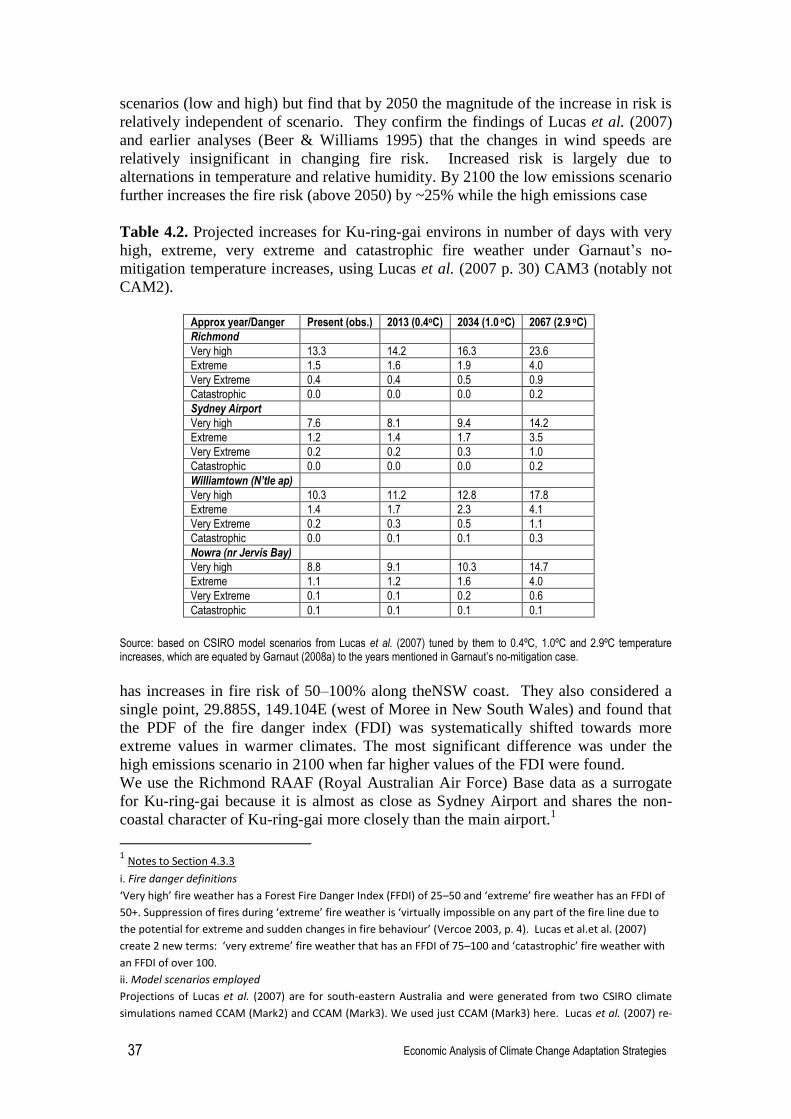
Economic Analysis of Climate Change Adaptation Strategies
37
scenarios (low and high) but find that by 2050 the magnitude of the increase in risk is
relatively independent of scenario. They confirm the findings of Lucas et al. (2007)
and earlier analyses (Beer & Williams 1995) that the changes in wind speeds are
relatively insignificant in changing fire risk. Increased risk is largely due to
alternations in temperature and relative humidity. By 2100 the low emissions scenario
further increases the fire risk (above 2050) by ~25% while the high emissions case
Table 4.2. Projected increases for Ku-ring-gai environs in number of days with very
high, extreme, very extreme and catastrophic fire weather under Garnaut‟s no-
mitigation temperature increases, using Lucas et al. (2007 p. 30) CAM3 (notably not
CAM2).
Approx year/Danger Present (obs.) 2013 (0.4oC) 2034 (1.0 oC) 2067 (2.9 oC)
Richmond
Very high 13.3 14.2 16.3 23.6
Extreme 1.5 1.6 1.9 4.0
Very Extreme 0.4 0.4 0.5 0.9
Catastrophic 0.0 0.0 0.0 0.2
Sydney Airport
Very high 7.6 8.1 9.4 14.2
Extreme 1.2 1.4 1.7 3.5
Very Extreme 0.2 0.2 0.3 1.0
Catastrophic 0.0 0.0 0.0 0.2
Williamtown (N’tle ap)
Very high 10.3 11.2 12.8 17.8
Extreme 1.4 1.7 2.3 4.1
Very Extreme 0.2 0.3 0.5 1.1
Catastrophic 0.0 0.1 0.1 0.3
Nowra (nr Jervis Bay)
Very high 8.8 9.1 10.3 14.7
Extreme 1.1 1.2 1.6 4.0
Very Extreme 0.1 0.1 0.2 0.6
Catastrophic 0.1 0.1 0.1 0.1
Source: based on CSIRO model scenarios from Lucas et al. (2007) tuned by them to 0.4ºC, 1.0ºC and 2.9ºC temperature increases, which are equated by Garnaut (2008a) to the years mentioned in Garnaut’s no-mitigation case.
has increases in fire risk of 50–100% along theNSW coast. They also considered a
single point, 29.885S, 149.104E (west of Moree in New South Wales) and found that
the PDF of the fire danger index (FDI) was systematically shifted towards more
extreme values in warmer climates. The most significant difference was under the
high emissions scenario in 2100 when far higher values of the FDI were found.
We use the Richmond RAAF (Royal Australian Air Force) Base data as a surrogate
for Ku-ring-gai because it is almost as close as Sydney Airport and shares the non-
coastal character of Ku-ring-gai more closely than the main airport.1
1 Notes to Section 4.3.3
i. Fire danger definitions
‘Very high’ fire weather has a Forest Fire Danger Index (FFDI) of 25–50 and ‘extreme’ fire weather has an FFDI of
50+. Suppression of fires during ‘extreme’ fire weather is ‘virtually impossible on any part of the fire line due to
the potential for extreme and sudden changes in fire behaviour’ (Vercoe 2003, p. 4). Lucas et al.et al. (2007)
create 2 new terms: ‘very extreme’ fire weather that has an FFDI of 75–100 and ‘catastrophic’ fire weather with
an FFDI of over 100.
ii. Model scenarios employed
Projections of Lucas et al. (2007) are for south-eastern Australia and were generated from two CSIRO climate
simulations named CCAM (Mark2) and CCAM (Mark3). We used just CCAM (Mark3) here. Lucas et al. (2007) re-

Economic Analysis of Climate Change Adaptation Strategies
38
Figure 4.4. Probability density function (PDF) of bushfire risk danger (FDI) at
29.885oS, 149.104
oE for each of a set of simulations (after Pitman et al. 2007)
4.4 Choosing a discount rate: How are non-market values included?
Discounting as a procedure involves expressing future and present values of particular
variables in a common unit so that decisions regarding possible courses of action in
the present can be made rationally. There is considerable ambiguity and indeed
controversy in the literature concerning the choice of discount rate to be used in
project evaluation. The basis of this controversy is twofold:
1. the relationship between discounting in a financial sense and discounting in an
economic sense
2. in the context of discounting in an economic sense, the magnitude of the
discount rate that should be used
scaled these to temperatures derived by CSIRO from the IPCC (2007) report, being 0.4-1.0
oC by 2020 and 0.7-
2.9oC by 2050 which they note allows for the full range of IPCC SRES scenarios of greenhouse gas and aerosol
emissions. Four regional projections are given for each climate simulation: 2020 low, 2020 high, 2050 low and
2050 high. Here we ignore the 2050 ‘low’ (0.7oC by 2050) in line with Garnaut (2008a).
iii. Caveats
The Lucas et al. (2007) methodology projects modelled changes from the various scenarios onto their observed
time series of temperature, rainfall, wind and relative humidity from 1973 to the present. This provides an
estimate based on observed past weather of future fire weather but does so by maintaining current, that is,
immediate past, time series characteristics. They assume that climate change will not alter the variability
observed over the past 30+ years. If this is not the case this methodology will not reproduce climate change
correctly.

Economic Analysis of Climate Change Adaptation Strategies
39
4.4.1 Discounting: financial versus economic
The key difference between discounting in a financial sense and discounting in an
economic sense is the variable whose present value is compared to its future value in
each case.
Financial discounting involves the comparison of explicit monetary flows – hence
discounting is necessary to convert future dollars (expected net earnings) into present
dollars so that a valid comparison can be made with known costs that must be
incurred in present dollar terms. It is only through appropriate discounting of future
net earnings that, for example, the question of the maximum price that should be paid
for an asset can be answered (for a given earnings profile the maximum justifiable
price is higher the lower the discount rate applied and vice versa).
Clearly it is desirable in a financial context to use a discount rate that reflects the cost
of capital or the cost of acquiring funds in some way – using a rate lower than the cost
of capital associated with the project implies that avoidable losses will be incurred. In
the context of an organisation with a binding budget constraint such as a local council,
from a financial perspective the use of artificially low discount rates for some projects
will necessitate reallocation of expenditure from other uses.
Discounting in the economic sense involves comparisons between future and present
welfare, and so raises a different set of questions.2
The paradigmatic case in
economics which is relevant to the current project is the choice among available
public investment projects, each of which involves the use of resources in the present
and the generation thereby of a path of welfare. The optimal investment is that which
maximises welfare, and the comparison of projects necessitates the conversion of
future welfare, or the welfare of future agents, into present-welfare equivalents. Such
conversion is discounting.
Unlike the financial case, there is no obvious „commonsense‟ value of the discount
rate to use in comparing welfare streams. The choice of discount rate is a choice
between the weight given to the interests of agents in the present and near future, and
the interests of agents further separated in time from the project‟s implementation.
High discount rates favour projects with immediate benefits and/or deferred costs, and
imply that the justifiable present cost (in terms of welfare foregone) of a given future
increase in welfare is low. Low discount rates render large present costs justifiable in
return for future welfare gains and so favour projects with deferred benefits and
immediate costs. Clearly the choice of discount rate in economic terms has a
significant, if not decisive, ethical component which has been the source of much
debate in the literature and, obviously, in response to the Stern (2006) and Garnaut
(2008c) reviews.
One could think of day-to-day public and private examples such as a public fire trail
providing a long term asset whose benefits accrue over time and where the capital
cost is high thereby attracting a lower priority when a high discount rate is used, while
2 Of course, welfare cannot be measured directly (if indeed it can be defined unambiguously!) and so it is standard
practice in economics to measure it by proxy in terms of monetary values such as Willingness To Pay and so on.
The superficial similarity between the two cases should not obscure the fundamental difference between them in
terms of purpose and interpretation.

Economic Analysis of Climate Change Adaptation Strategies
40
upgrading a private house to comply with recent changes to the Building Code of
Australia has a lower unit cost and perceived immediate benefit. Questions then arise
regarding public versus private projects and common good versus private benefits.
4.4.2 Choosing a discount rate from an economic perspective
In order to explain the choice of discount rate in the Garnaut Review (2008c), it is
necessary to outline the way in which economists conceptualise the problem. Such
conceptualisation clarifies the assumptions and caveats in the Review that underpin
the final choice.
In economic theory, welfare means the satisfaction of preferences. By definition, an
increase in welfare for an agent entails moving to a more preferred outcome.
Preferences are defined in terms of consumption, so an increase in welfare is defined
as a move to a more preferred combination of goods consumed.
Economists represent preferences for technical purposes through the use of a utility
function:
)(cuU (1)
where U is utility, an index that indicates the place of a given consumption
combination (c) relative to others (higher utility numbers indicating more preferred
combinations). The typical investment project will imply a consumption trajectory
over the given time horizon (possibly infinite) giving rise to a total welfare effect of:
0
0 )( dtcuU t (2)
whereU0 is the total utility of the stream of c‟s over time, evaluated in period 0 (that
is, the present, in which the project will be implemented).
As was recognised by Ramsay (1928) there is a technical need for discounting (which
he decried on ethical grounds) if a choice is to be made among possible consumption
paths (that is, projects). The zero discount rate case depicted involves summing finite
quantities over an infinite horizon; project choice would then require an illegitimate
comparison of infinites. Discounting of utilities converts the stream of utilities into a
declining geometric series, which therefore has a finite sum:
0
0 )( dtecuU tt
(3)
Given the differing consumption paths, the choice of project will now be determined
by the value taken by the discount rate applied to utilities (θ).
It is at this point that the ethical/governance aspects of the discount rate choice begin
to bite. The first issue concerns the role of pure time preference or intrinsic
discounting. This involves assigning different weights to consumption baskets purely
on the basis that they will occur at different points in time. In other words, a positive

Economic Analysis of Climate Change Adaptation Strategies
41
rate of pure time preference implies that a given quantity of consumption to be
experienced n periods in the future would be considered inferior to the same quantity
experienced now, ceteris paribus.
Philosophers such as Rawls (1971) and Parfit (1984) hold pure time preference to be
inconsistent with individual rationality, a fairly standard position in the political
philosophy and distributive justice literatures. Economists are more circumspect on
the issue (the basic textbook model of the intertemporally optimising consumer does
not assume zero subjective time preference, for example) but generally concur with
the philosophers that pure time preference is unjustifiable in terms of collective
choice. That is, a government considering a choice among investment projects ought
not treat the welfare of future generations as less important than that of those currently
alive simply because of the displacement in time. This view is encapsulated through
one of the principles of sustainability – intergenerational equity.
This position is reflected in the Garnaut report in which a baseline value of zero is
chosen for pure time preference, with only a slight adjustment made to allow for the
possible occurrence of an extinction event. A discount rate of zero would imply that
the welfare of the current generation is weighted equally to that of a billion years in
the future; the 0.05% rate set by Garnaut means that the welfare of people around
1400 years in the future is worth half of that of people alive today. For more relevant
timeframes (such as 100 years) the 0.05% rate implies only a marginal decrease
(around 5%) in the importance of future welfare.3
However, where future generations are expected to be better off than present agents
there is scope for discounting on grounds other than pure time preference. In other
words, if future agents will consume more than current agents then the sacrifices of
current agents on behalf of future agents ought to be lower notwithstanding that the
welfare of agents is considered to be of equal importance regardless of the generation
in which they live.
In order to explain the way in which economic growth projections (that is, rising
consumption over time) lead to a positive discount rate, it is necessary to delve in
more detail into the form of utility functions typically used in economic analysis.
Figure 4.5 illustrates a typical utility function defined over consumption. The
curvature of the function reflects the assumption of diminishing marginal utility, the
decreasing rate of increase in the utility number as consumption increases. This
assumption has a number of implications, of which one is particularly notable in terms
of the debate over the choice of discount rate to be used in Garnaut-type exercises.
3 By way of comparison, with a 1% rate of discount the welfare of current agents is worth twice that of those in 69
years time and nearly three times that of agents a century hence.

Economic Analysis of Climate Change Adaptation Strategies
42
Figure 4.5. Typical utility function
Figure 4.5 shows that for consumption quantities c1 and c2 the corresponding utility
numbers are U1 and U2 respectively (c2 is thus preferred to c1). The line segment
connecting the points on the curve corresponding to c1 and c2 represents the possible
linear combinations of c1 and c2. If the linear weights are interpreted as probabilities,
p and (1-p), then the line segment marks out the expected values of possible simple
lotteries over c1 and c2 for all values of p. For the case in which p=0.5, the expected
value of the lottery (as shown in 4.7) is the arithmetic mean of c1 and c2.
The expected value (EV) of the lottery, if experienced as a definite quantity of
consumption has a utility value of U(EV). However the utility of the lottery (that is, a
50% chance of either c1 or c2), the expected utility (EU) of the lottery, is EU, which is
less than U(EV). As the expected utility is less than the utility of the expected value,
the agent would prefer the EV amount for certain to the EV amount on average. The
agent is risk averse.
Clearly the curvature of the utility function is the key factor in terms of diminishing
marginal utility and the degree of risk aversion. The fact that marginal utility is
assumed to be decreasing as consumption increases immediately suggests a role for
discounting – on the assumption that agents share a common utility function across
time, rising consumption over time implies, unit for unit, progressively smaller
increases in welfare. This in turn suggests that current welfare sacrifices should not
rise pari passu with associated future welfare gains – future welfare should be
discounted because a given increment in consumption has a greater welfare impact in
the present than it does in the future if consumption is rising.
In order to determine the rate at which welfare should be discounted on this basis, we
need to make more specific assumptions about the curvature of the utility function. As
utility functions of the type typically used are unique only up to a positive linear
transformation, the absolute values of changes in marginal utilities cannot be used to
define curvature adequately (that is, U=u(c) and U=a[u(c)]+b represent the same set
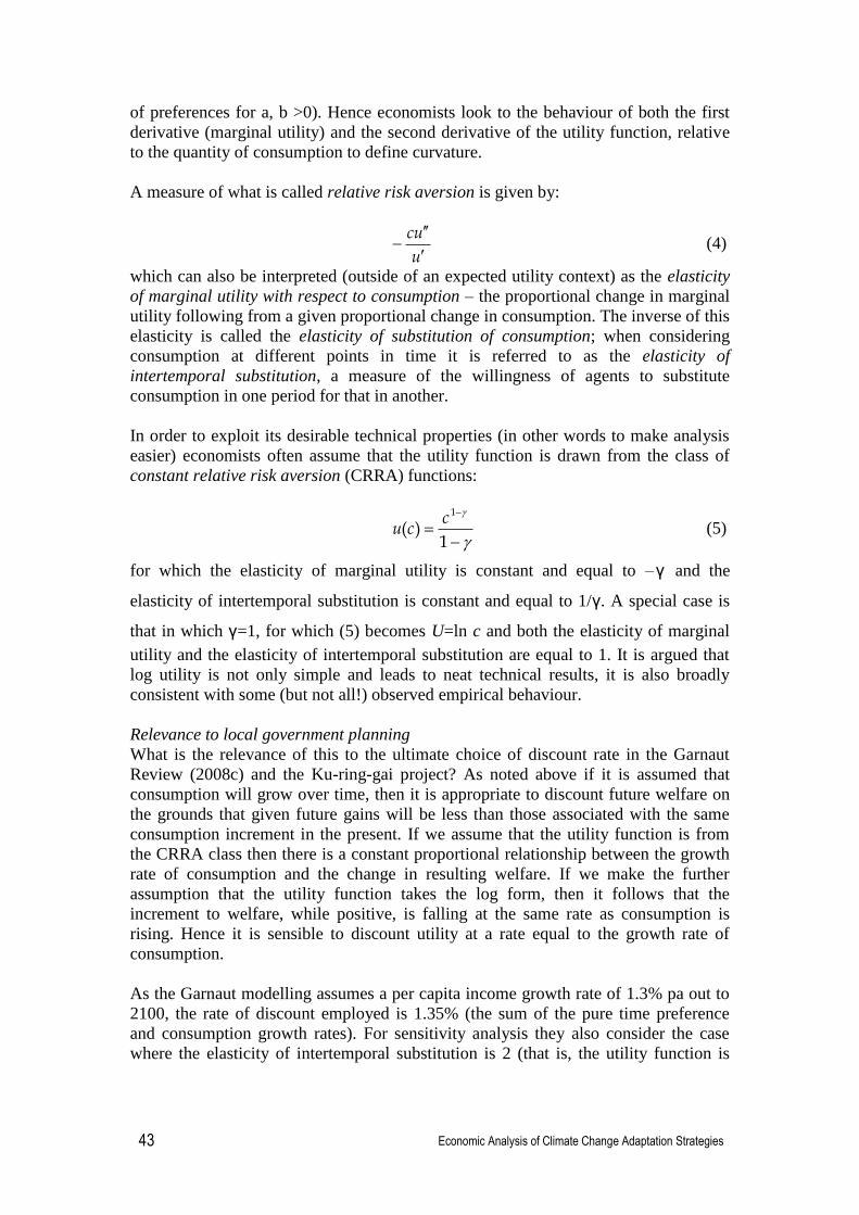
Economic Analysis of Climate Change Adaptation Strategies
43
of preferences for a, b >0). Hence economists look to the behaviour of both the first
derivative (marginal utility) and the second derivative of the utility function, relative
to the quantity of consumption to define curvature.
A measure of what is called relative risk aversion is given by:
u
uc
(4)
which can also be interpreted (outside of an expected utility context) as the elasticity
of marginal utility with respect to consumption – the proportional change in marginal
utility following from a given proportional change in consumption. The inverse of this
elasticity is called the elasticity of substitution of consumption; when considering
consumption at different points in time it is referred to as the elasticity of
intertemporal substitution, a measure of the willingness of agents to substitute
consumption in one period for that in another.
In order to exploit its desirable technical properties (in other words to make analysis
easier) economists often assume that the utility function is drawn from the class of
constant relative risk aversion (CRRA) functions:
1)(
1ccu (5)
for which the elasticity of marginal utility is constant and equal to –γ and the
elasticity of intertemporal substitution is constant and equal to 1/γ. A special case is
that in which γ=1, for which (5) becomes U=ln c and both the elasticity of marginal
utility and the elasticity of intertemporal substitution are equal to 1. It is argued that
log utility is not only simple and leads to neat technical results, it is also broadly
consistent with some (but not all!) observed empirical behaviour.
Relevance to local government planning
What is the relevance of this to the ultimate choice of discount rate in the Garnaut
Review (2008c) and the Ku-ring-gai project? As noted above if it is assumed that
consumption will grow over time, then it is appropriate to discount future welfare on
the grounds that given future gains will be less than those associated with the same
consumption increment in the present. If we assume that the utility function is from
the CRRA class then there is a constant proportional relationship between the growth
rate of consumption and the change in resulting welfare. If we make the further
assumption that the utility function takes the log form, then it follows that the
increment to welfare, while positive, is falling at the same rate as consumption is
rising. Hence it is sensible to discount utility at a rate equal to the growth rate of
consumption.
As the Garnaut modelling assumes a per capita income growth rate of 1.3% pa out to
2100, the rate of discount employed is 1.35% (the sum of the pure time preference
and consumption growth rates). For sensitivity analysis they also consider the case
where the elasticity of intertemporal substitution is 2 (that is, the utility function is

Economic Analysis of Climate Change Adaptation Strategies
44
U=(1/2)(c)1/2
) so that the discount rate used is 2.65% (2 times the growth rate plus the
0.05% pure time preference rate).4
4.4.3 Choice of rate for the Ku-ring-gai project
The key question is how far, if at all, we wish to diverge from the Garnaut
assumptions. Specifically:
Are there grounds for assuming that incomes in Ku-ring-gai will rise more
quickly or more slowly than the national average out to 2100?
Are there grounds for assuming different forms for the utility function?
Are there grounds for assuming a higher or lower rate of pure time preference
than is used in the Garnaut report?
The pure time preference question is involved and complicated. On the one hand the
principle of non-discrimination among generations has intuitive appeal, and yet on the
other pure time preference does appear to be an identifiable aspect of individual
behaviour (and hence a characteristic of the preferences of each generation) and so
arises the question of whether the „authoritarian‟ response (Marglin 1963) of
overriding those preferences in a democratic context is justifiable. Furthermore, the
argument is based on the assumption of the homogeneity of preferences across time,
the coherence of which is questioned by some commentators (Ball 1985). Finally we
might consider whether Ku-ring-gai Council functions as the guardian of future
generations of ratepayers in the same way that a national government does with
regard to future citizens according to the advocates of low social discount rates.
The choice of the form of utility function is typically driven by analytical convenience
as noted, and the empirical evidence, such as it is, is mixed regarding the „fit‟ of log
utility. The choice of a different form could not really be justified empirically for Ku-
ring-gai simply due to the difficulty of testing involved. In any case the decision to
use a different form of the utility function and the decision to use a higher social
discount rate are effectively one and the same.
Finally the issue of growth rates is also difficult. Note that it is important not to
confuse levels and growth rates. Ku-ring-gai almost certainly has an above average
per capita income but are there grounds for predicting that income will grow faster
than average over time? In the absence of such grounds it might be sensible to stick
with the Garnaut rate. Hence, in terms of the social discount rate used there may be no
obvious grounds for departing from the rates used by Garnaut.
As for the conflict between the social discount rate and the rate to be used in a
financial sense, there are few concrete indications to be gleaned from either theory or
practice. The Garnaut Review (2008c) notes the distinction, using the positive-
normative distinction, and argues that it is appropriate to use market rates of interest
for discounting when analysing private market activity such as pricing emissions
permits, and to use social discount rates, which should be lower, when comparing
utility outcomes. For the current project there might be grounds to argue that
4 The intuition behind the higher discount rate is straightforward. For the non-log utility function, marginal utility
declines at a slower rate as consumption grows. Hence, future generations are made better off by any given
increment to consumption relative to the log utility case. Thus future utility must be discounted more strongly for
any rate of consumption growth.

Economic Analysis of Climate Change Adaptation Strategies
45
appropriate market rates be used in assessing the financial viability of projects while
appropriate non-market rates be used to decide among financially viable activities.
Public sector investment has a duty to act upon future risk, for example the 1 in
100,000 year flood that may entail a low discount rate independent of population
growth or increased prosperity. The mechanics certainly remain unclear, but that is
true of the approach taken by government agencies.
4.5 Ranking system for prioritising various adaptation options
In this section we discuss the use of a ranking system which may be more useful to
local councils than conventional CBA. The system includes a methodology for netting
the impacts within each option, using Borda counts developed by Jean Charles de
Borda in 1781.
4.5.1 Why not conventional CBA?
Cost Benefit Analysis (CBA) identifies present and future gains and losses incurred
by a particular action in the present. It usually applies to financial cases where dollar
values exist. Consistent, transparent and replicable, CBA is embraced by local
councils; however, when used to value environmental or social impacts, it becomes
unrealistically expensive and inaccurate in establishing monetary values for non-
market values. Putting a dollar value on non-market public good has never been
satisfactorily achieved. What is the value of a clear sky or a beautiful mountain? What
is the value of your child‟s life? Questionnaires are prepared asking, for example,
willingness to pay for national park entry which then becomes a surrogate for the
value of a national park.
Climate adaptation actions demand immediate attention and this urgency is largely
accepted since the Nobel Peace Prize was awarded for the IPCC Fourth Assessment
Report (AR4) and to Al Gore in 2007. An attempt to use CBA for Triple Bottom Line
planning may fail in the environmental case but will almost certainly fail in the social
case, where putting dollar values to life, health and pain will be contentious. An
incomplete or partial CBA will necessarily reflect the bias of those commissioning the
analysis.
4.5.2 A ranking system as preferred to CBA
A ranking system can take into account both financial and social ordering. Rankings
can be enriched by expert opinion, council officer experience and training, local
knowledge, and scientific evidence.
According to Kenneth J Arrow (1950), the only method of passing from individual
preferences to social preferences that is satisfactory and that is defined for a wide
range of individual orderings is either imposed or dictatorial. Arguably Ku-ring-gai
Council, with its Mayor and elected Councillors as democratic representatives of its
constituency (who guide officials acting as service providers to the community) is
reasonably in a position to take „right‟ decisions on behalf of the community.
4.5.3 Ranking the three cases of TBL
Ranking in the financial case is purely based on dollar returns and takes into
consideration maximum net benefits for each choice. A strategy showing most net
benefit will be ranked first. Environmental and social ranking are left to the discourse

Economic Analysis of Climate Change Adaptation Strategies
46
of Council‟s experts. This system of ordering social and environmental impacts
resolves the dilemma of choosing a discount rate inasmuch as no dollar values need
be devised for non-market public goods. Accompanying the rankings by qualitative
statements describing the costs and benefits and reasons for the ranks assigned would
help to make the cases transparent and reduce discrepancies.
4.5.4 Borda counts for selecting the most appropriate adaptation strategy
Ranking scores are based on the order of preference of Council and the community.
Final ranking for the most socially, economically and environmentally viable option is
obtained using Borda count votes. Saari et.al. (2006) support Borda count as a fair
voting system compared to other prevailing systems such as Condorcet winner.
Suppose there are n options which have been ranked in order of preference. The
Borda method assigns the numeric values n-1, n-2, … 0 respectively to the first,
second, … last ranked options in columns. The option with the greatest total number
of Borda votes in rows will be the winning option. The following example, Table 4.3,
illustrates how the Borda count scoring system works.
Table 4.3. Research Work in Progress: Hypothetical voting and Borda counts for the
three TBL cases: social, environmental and financial*
Options Social
Ranks/ (score) Environmental Ranks/(score)
Financial Ranks/(score)
Borda Count
Option 1: building fire trails 1 (4) 3 (2) 2 (3) 9
Option 2: fire control center 2 (3) 1 (4) 4 (1) 8
Option 3: rezoning land in risk areas
3 (2) 2 (3) 1 (4) 9
Option 4: Increase number of prescribed burns
4 (1) 4 (1) 3 (2) 4
Option5: community education program
5 (0) 5 (0) 5 (0) 0
*Work in progress, not to used for decision-making purposes
In this example Option 1 and Option 3 have equal highest Borda counts; therefore
Council may decide the preferred option. Where one option attracts the highest score
it is selected as the best adaptation option.
4.6 Economic Models and Loss Distribution Approach (LDA)
4.6.1 Introduction
The following section outlines an approach for quantifying potential losses from
catastrophic events like storms, droughts or bushfires that may increase owing to
climate change. There are several problems in establishing an appropriate quantitative
model for this task. First, the number of observations is sparse, particularly at the
local scale. This presents difficulties in calibrating the distribution and models
inasmuch as parameter estimates of distribution are sensitive to the observations.
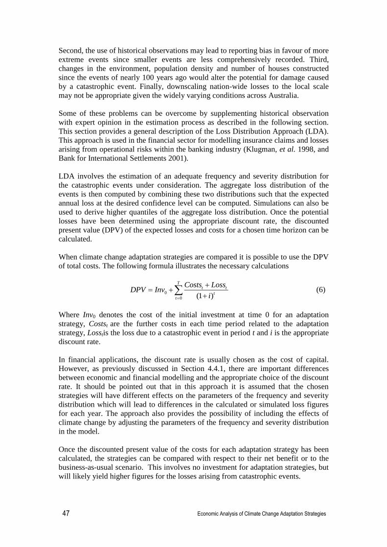
Economic Analysis of Climate Change Adaptation Strategies
47
Second, the use of historical observations may lead to reporting bias in favour of more
extreme events since smaller events are less comprehensively recorded. Third,
changes in the environment, population density and number of houses constructed
since the events of nearly 100 years ago would alter the potential for damage caused
by a catastrophic event. Finally, downscaling nation-wide losses to the local scale
may not be appropriate given the widely varying conditions across Australia.
Some of these problems can be overcome by supplementing historical observation
with expert opinion in the estimation process as described in the following section.
This section provides a general description of the Loss Distribution Approach (LDA).
This approach is used in the financial sector for modelling insurance claims and losses
arising from operational risks within the banking industry (Klugman, et al. 1998, and
Bank for International Settlements 2001).
LDA involves the estimation of an adequate frequency and severity distribution for
the catastrophic events under consideration. The aggregate loss distribution of the
events is then computed by combining these two distributions such that the expected
annual loss at the desired confidence level can be computed. Simulations can also be
used to derive higher quantiles of the aggregate loss distribution. Once the potential
losses have been determined using the appropriate discount rate, the discounted
present value (DPV) of the expected losses and costs for a chosen time horizon can be
calculated.
When climate change adaptation strategies are compared it is possible to use the DPV
of total costs. The following formula illustrates the necessary calculations
0
0 (1 )
Tt t
tt
Costs LossDPV Inv
i
(6)
Where Inv0 denotes the cost of the initial investment at time 0 for an adaptation
strategy, Costst are the further costs in each time period related to the adaptation
strategy, Losstis the loss due to a catastrophic event in period t and i is the appropriate
discount rate.
In financial applications, the discount rate is usually chosen as the cost of capital.
However, as previously discussed in Section 4.4.1, there are important differences
between economic and financial modelling and the appropriate choice of the discount
rate. It should be pointed out that in this approach it is assumed that the chosen
strategies will have different effects on the parameters of the frequency and severity
distribution which will lead to differences in the calculated or simulated loss figures
for each year. The approach also provides the possibility of including the effects of
climate change by adjusting the parameters of the frequency and severity distribution
in the model.
Once the discounted present value of the costs for each adaptation strategy has been
calculated, the strategies can be compared with respect to their net benefit or to the
business-as-usual scenario. This involves no investment for adaptation strategies, but
will likely yield higher figures for the losses arising from catastrophic events.

Economic Analysis of Climate Change Adaptation Strategies
48
In the following two sections we will discuss the Loss Distribution Approach (LDA)
and additional statistical techniques that are relevant for the modelling of losses
arising from catastrophic events like storms, droughts or bushfires. Preliminary results
on estimated distributions and bushfire loss are then given in the results section.
4.6.2 The Loss Distribution Approach (LDA)
The LDA is a statistical approach for generating aggregate loss distribution. This
section provides the algorithms that can be used to compute the aggregate loss
distribution and illustrates the calculation of extreme quantiles for losses based on the
generated aggregate loss distribution. As mentioned above this approach is
particularly popular in the financial industry (Klugman et al. 1998, and Bank for
International Settlements 2001). Researchers commonly use the Poisson distribution
for frequency and the Lognormal distribution for severity.
To compute the probability distribution of the aggregate loss from bushfires over one
year, it is necessary to estimate the probability distribution function of the single event
loss and its frequency for one year. With the benefit of internal and external data (data
generated outside the current research project for different purposes and adapted for
the present project, for example, bushfire losses experienced by other regions of
Australia) supplemented by expert opinion, researchers may estimate the probability
distribution function of residential property loss and the bushfire frequency over one
year. Then it is possible to compute the cumulative residential property loss for one
year or longer.
In LDA, the loss severity distribution and loss frequency distribution are assumed to
be independent. Thus, the cumulative loss for one year is expressed as
1
N
i
i
G X
(7)
whereN is the annual number of events modelled as a random variable from a discrete
distribution and , 1,...,iX i N , are severities of the event modelled as independent
random variables from a continuous distribution. Modelling frequency and severity of
losses is a well-known actuarial technique (Klugman et al. 1998).
Monte Carlo simulation is normally used to compound the severity and frequency
distribution and calculate the aggregate losses from an event type (Fishman 1996).
The simulation algorithm to generate an annual loss distribution is as follows:
1. Take a random draw from the frequency distribution: suppose this simulates N
events per year.
2. Take N random draws from the severity distribution: denote these simulated loss by
L1, L2, …, LN
3. Sum the n simulated losses to obtain an annual loss X = L1+L2+…+LN
4. Return to step 1, and repeat k times (usually the number of simulation runs is
chosen to be k=5000,10000 or even higher). Then we will obtain X1, X2,…,Xk where

Economic Analysis of Climate Change Adaptation Strategies
49
k is a very large number that enables us to derive a distribution for the aggregate
losses.
Thus, using the LDA, we can compute the expected loss and loss at a confidence level
of the event for one year or longer. The expected loss EL and the loss at a
confidence level L( ) are then defined by
0
( )EL xdG x
and
( ) inf{ | ( ) }L x G x . (8)
The expected loss is the expected value of the aggregate loss distribution function G
whereas the loss at confidence is the quantile for the level . By using Monte
Carlo simulation, we can generate the aggregate loss distribution of the event and
obtain, for example, the quantiles at 90% and 99% confidence levels. The accuracy of
the estimation depends on the adequacy of the parameter estimates but also on the
number of simulations in the Monte Carlo approach (Fishman 1996). Thus a high
number of simulations is recommended.
As mentioned above, comparing adaptation strategies over a longer period of time
requires simulations for a longer period of time. The algorithm presented here can
easily be adjusted for this purpose and the simulated losses for each year t=1,..,T can
be discounted using the specified discount rate i. In this case it may be necessary to
adjust the model parameters of the frequency and severity distribution over time, if,
for example, an increase in the frequency or severity of bushfires is expected over that
period of time. Assuming that the effects on parameter estimates and changes over
time can be quantified correctly, it is then possible to gain more realistic figures for
the costs or benefits of different strategies.
2.6.3 Statistical Modelling and Simulation
The frequency of events is usually modelled by a discrete probability distribution
(such as Bernoulli, Binomial, Poisson or Geometric distributions). Discrete
distributions apply to a random variable whose set of possible values is finite or
countable. Hence the frequency of an event, as a countable discrete random variable,
can be modelled by a discrete distribution.
One problem for the estimation procedure is that often data on severities contain a
substantial proportion of zeros; for example the number of damaged houses from a
bushfire is zero for approximately 70% of the recorded bushfires. In this case, a first
attempt to model the severity by a continuous distribution using all the observations
including the zeros might not provide an adequate fit. Data with many zeros violates
the underlying assumption of such distributions. Therefore, in this case a so-called
mixture model may applied to model these zero-inflated data. In general, mixture
models characterize zero-inflated data as a function of two distributions (Y=VB).
First, B means the likelihood of zero or positive outcomes, which can be characterised
using Bernoulli distribution. Then, the positive outcomes are independently modelled
as V. This type of approach to model zero-inflated data was first discussed by
Aitchison (1955) and has been used to model mackerel egg counts (Pennington 1983),
health statistics (Zhou & Tu 2000), and air contaminant levels (Tu 2002). A
generalized mixture model can be characterized as follows

Economic Analysis of Climate Change Adaptation Strategies
50
( | ) 1 ( ) 0
( ) ( | ) 0
f y y
g y y
(9)
where0
( | ) 1g y dy
In a later section we will suggest using the Lognormal distribution to model the
positive data: the resulting distribution including the zeros is often referred to as the Δ
-distribution or Delta distribution.
An example follows of the simulation process based on the loss distribution approach
being conducted to generate a probability distribution of the DPV of aggregate losses
arising from destroyed houses for a period of several years. Note that in this example
only house damage is modelled; other losses arising from bushfires are not
considered. The simulation is based on PerilAUS bushfire data for NSW where the
value of a „house equivalent‟ is assumed to be AUD $440,000.
Assume that the number of severe bushfires per year can be modelled by a Poisson
distribution with parameter λ=3.8. This means that the average number of severe
bushfires per year is 3.8. The probability distribution for the number is provided in
Figure 4.6.
Figure 4.6. Probability distribution for number of severe bushfires in NSW based on
a Poisson distribution with parameter λ=3.8.

Economic Analysis of Climate Change Adaptation Strategies
51
Further assume that the fraction of severe bushfires that actually leads to losses from
destroyed houses is 33% and can therefore be modelled by a Bernoulli distribution
with parameter p=0.33.
Finally assume that if the bushfire actually leads to house damage, the number of
houses destroyed can be modelled by a Lognormal distribution with parameter μ=1.67
and σ=1.39. This corresponds to a mean of approximately 14 houses destroyed. The
corresponding probability distribution is provided in Figure 4.7.
Figure 4.7. Probability distribution for the number of destroyed houses in a severe
bushfire in NSW based on a Lognormal distribution with parameters μ=1.67 and σ
=1.39. The blue bars represent the simulated Lognormal distribution with parameters
μ=1.67 and σ=1.39 while the orange line represents the theoretical Lognormal
distribution.
The simulation process is conducted as follows:
1. For each year t=1,…,T first draw a random number from the Poisson
distribution with parameter λ=3.8. This corresponds to the number Ntof
fires in year t. Assume for example that the generated random number is
Nt=3 corresponding to three bushfires in year t.
2. For each of the bushfires, in the simulation process it needs to be
determined whether it is a bushfire that destroyed houses or not. In our
example, for each of the three fires n=1,2,3 a Bernoulli random number Zn

Economic Analysis of Climate Change Adaptation Strategies
52
is drawn to decide whether houses were affected or not. For the example
the probabilities are 0.67 for the result 0 (no house affected) and 0.33 for
the result 1 (houses are destroyed). Assume that we get Z1=0, Z2=1 and
Z3=0. So only the second fire was one that destroyed a number of homes.
3. Simulate the severity for the fires that destroyed houses from the
Lognormal distribution. In our example this means that for the second
bushfire we simulate a random number from the Lognormal distribution
with parameters μ=1.67 and σ=1.39. Assume the outcome is 6.32. Then
the calculated loss from destroyed houses for year t is Gt=AUD 2,780,800.
4. Repeat steps 1) to 3) for each year and determine the corresponding figures
Gt for t=1,…,T.
5. Calculate the DPV of the losses from destroyed houses by discounting the
loss figures Gt with an appropriate discount rate:1 (1 )
Tt
tt
GDPV
i
.
6. Repeat steps 1) to 6) many times (e.g. n=5000 or n=10,000) to derive a
simulated probability distribution of the losses that can be used to calculate
expected losses or the Value-at-Risk at higher quantiles e.g. 95%, 99%,
etc.
Figure 4.8 illustrates such a simulated probability distribution for the potential losses
from destroyed houses. For simplicity, in this example only a time horizon of one year
was considered and n=5000 simulations were run.
Figure 4.8. Simulated probability distribution for the bushfire losses arising from
destroyed houses for n=5000 simulations in a one year period.

Economic Analysis of Climate Change Adaptation Strategies
53
This algorithm can be applied to different kinds of catastrophic risks or losses and can
be altered to include climate change scenarios or adaptation scenarios. For example,
increasing or decreasing frequencies or severities can be included in the simulation
procedure based on the assumptions about the effects of climate change or adaptation
strategies on the distributions.
The estimation of frequency and severity distribution, especially for low frequency
high impact bushfire losses, is a challenging task. Local Ku-ring-gai bushfire records
contain only a very few high impact events. Because sufficient sample data is required
for producing a meaningful estimation, later applications will incorporate external
data, that is, bushfire losses experienced by other regions in Australia, and expert
opinion. Here, bushfire data from the PerilAUS database is considered to be external
data. Expert opinion regarding frequency and severity of losses can be incorporated
in the model using Bayesian estimation techniques. The next section provides the
general framework and some information on how, in a practical application, expert
opinion and empirically observed data can be combined to estimate frequencies and
severities in the LDA.
4.7 Using Bayesian inference methods for the quantification of losses
4.7.1 Introduction
In order to estimate an adequate probability distribution for the potential losses from
catastrophic events on a local scale, it might be necessary to take into account
information beyond the often sparse historical data. This could include relevant
external data and expert opinion on the probability and severity of such events.
Considering the often small number of observations that will be available, it can be
important to have such expert judgement, often referred to as scenario analysis,
incorporated into the model.
The following statistical background illustrates how different sources of information –
particularly historical data on losses from catastrophic events and expert judgement –
can be combined. Here we follow an approach using Bayesian estimation as initially
suggested in Shevchenko and Wüthrich (2006) for the quantification of operational
risks in the banking industry. As mentioned above in the Loss Distribution Approach
suggested by the Basel Committee of Banking Supervision (a standing committee of
the Bank for International Settlements), a very similar problem of estimation of
frequency and severity distributions often based on low-frequency-high-severity data
is required. To overcome these difficulties, according to the Basel Committee of
Banking Supervision, it is mandatory to include scenario analysis in the model for risk
quantification to meet regulatory requirements. Here, scenario analysis gives a rough
quantitative assessment of risk frequency and severity distributions based on expert
opinion. Scenario analysis is subjective and wherever possible should be combined
with actually observed loss data. In recent years Bayesian inference has gained some
popularity in the insurance and financial industry for combining such sources of
information. For an introduction to Bayesian inference methods and their application
to insurance and finance, refer to Berger (1985), Bühlmann and Gisler (2005) or
Rachev et al. (2008).

Economic Analysis of Climate Change Adaptation Strategies
54
Generally, Bayesian techniques allow for structural modelling where expert opinion is
incorporated into the analysis via the specification of so-called prior distributions for
the model parameters. The original parameter estimates are then updated by the data
as they become available. Additionally, the expert may reassess the prior distributions
at any point in time if new information becomes available on, for example, climate
change, or the effects of climate change on the frequency and severity of catastrophic
storm, drought or bushfire events. To our knowledge, this technique has not been used
to quantify the risk from such catastrophic losses, particularly notat the local scale.
The next section gives a brief description of the technique within the context of
application to risks arising from natural disasters like bushfires and storms. The next
chapter, Results, will illustrate our preliminary results on parameter estimation of the
frequency and severity distribution and potential losses from bushfires at the local
scale in the Ku-ring-gai Local Government Area.
4.7.2 Bayesian techniques
Let us first consider a random vector of observations ),...,,( 21 nxxxX whose density
h(X|θ) is given for a vector of parameters θ= (θ1, θ2, . . . , θK). The big difference
between the classical and the Bayesian estimation approach is that in the latter both
observations and parameters are considered to be random. Let further π(θ) denote the
density distribution of the uncertain parameters, which is often also called the prior
distribution. The Bayes‟ theorem can then be formulated as:
ö( , ) ( | ) ( ) ( | ) ( )h X h X X h X (10)
Here, ( , )h X is the joint density of the observed data and parameters, ö( | )X is the
density of the parameters based on the observed data X, ( | )h X is the density of the
observations given the parameters θ. Finally, h(X) is a marginal density of X that can
also be written as
h(X) = h(X|θ)π(θ) dθ (11)
Note that in the Bayesian approach the prior distribution π(θ) generally also depends
on a set of further parameters called hyper parameters. As mentioned above, these
parameters and the prior distribution can also be updated if new information on
climate change and its effect on catastrophic events become available. Overall, the
approach is capable of combining the prior assessment of an expert on the frequency
and severity of events and actually observed data in the considered local area. It also
enables the modeller to adjust the distribution based on different adaptation scenarios
and their effects on the risk by using the expert judgement on the effect of such
strategies. In the following section, we will briefly explain how, based on a prior
judgement of the expert on frequency and severity, the estimates can be updated when
additional information on losses from events becomes available.
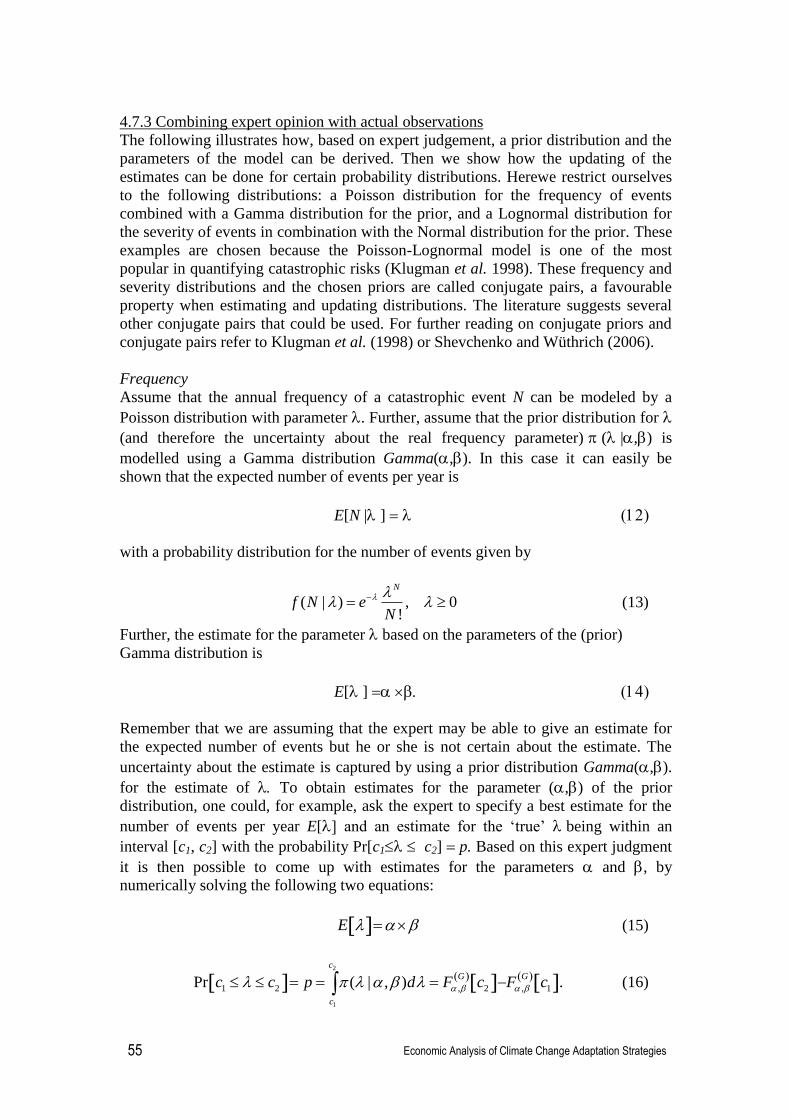
Economic Analysis of Climate Change Adaptation Strategies
55
4.7.3 Combining expert opinion with actual observations
The following illustrates how, based on expert judgement, a prior distribution and the
parameters of the model can be derived. Then we show how the updating of the
estimates can be done for certain probability distributions. Herewe restrict ourselves
to the following distributions: a Poisson distribution for the frequency of events
combined with a Gamma distribution for the prior, and a Lognormal distribution for
the severity of events in combination with the Normal distribution for the prior. These
examples are chosen because the Poisson-Lognormal model is one of the most
popular in quantifying catastrophic risks (Klugman et al. 1998). These frequency and
severity distributions and the chosen priors are called conjugate pairs, a favourable
property when estimating and updating distributions. The literature suggests several
other conjugate pairs that could be used. For further reading on conjugate priors and
conjugate pairs refer to Klugman et al. (1998) or Shevchenko and Wüthrich (2006).
Frequency
Assume that the annual frequency of a catastrophic event N can be modeled by a
Poisson distribution with parameter . Further, assume that the prior distribution for
(and therefore the uncertainty about the real frequency parameter)(|,) is
modelled using a Gamma distribution Gamma(,). In this case it can easily be
shown that the expected number of events per year is
E[N |]
with a probability distribution for the number of events given by
( | ) , 0!
N
f N eN
(13)
Further, the estimate for the parameter based on the parameters of the (prior)
Gamma distribution is
E[]
Remember that we are assuming that the expert may be able to give an estimate for
the expected number of events but he or she is not certain about the estimate. The
uncertainty about the estimate is captured by using a prior distribution Gamma(,).
for the estimate of To obtain estimates for the parameter (,) of the prior
distribution, one could, for example, ask the expert to specify a best estimate for the
number of events per year E[] and an estimate for the „true‟ being within an
interval [c1, c2] with the probability Pr[c1 c2] p. Based on this expert judgment
it is then possible to come up with estimates for the parameters and , by
numerically solving the following two equations:
E (15)
2
1
1 2 , 2 , 1Pr ( | , )
c
G G
c
c c p d F c F c . (16)

Economic Analysis of Climate Change Adaptation Strategies
56
The estimates of (,) and can then be considered as a starting point for modelling.
If actual observations on the number of events N1, N2 ,…,Nn for the periods 1,…, n
are available the parameters and , can then be updated according to the following
formulas (see Shevchenko and Wüthrich (2006) for the derivation):
1
ön
i
i
N
(17)
ö /(1 )n (18)
Then, the expected number of events, given the prior distribution and past
observations can be calculated as:
11 0
öö| | (1 )1
n
i
in
N
E N N E N wN wn
(19)
Here, 1
1 n
i
i
N Nn
is the estimate of using the observed number events only,
0 is the estimate of using the prior distribution only and 1/
nw
n
is the
so-called credibility weight that is used to combine the two estimates. Obviously, as
the number of period n increases, the credibility weight w increases, too. Therefore,
the more observations we have, the greater will be the weight assigned to the
estimator based on the observed events, while the smaller becomes the weight that is
attached to the expert opinion estimate. This makes the approach very attractive for
situations were the number of actually observed events is rather small, such as
bushfires and storms on a local scale. Here, despite the small number of observations,
combining an initial expert opinion with the actually observed number of events per
period should yield an appropriate estimate for the frequency.
Severity
For severity distribution, we assume the severity or magnitude of a catastrophic event
can be modeled using a Lognormal distribution LN(,Further assume that the
parameter is known while is uncertain and can be modeled by using the Normal
distribution as the appropriate prior distribution for is N(. Note that in this
case, given the prior distribution, the probability distribution for the loss arising from
a catastrophic event is
2
22
ln1( | , ) exp
22
xf x
x
(20)
while the expected value of the losses is
21| , ( , ) exp( )
2E X M . (21)

Economic Analysis of Climate Change Adaptation Strategies
57
Similar to the approach for frequency, the expert may be able to specify the best
estimate of the expected loss E[M(,)] as well as some information on the
uncertainty of this estimate by providing the probability that the true expected loss
lies in the interval [c1, c2], P[c1 c2] p. Then, by numerically solving the
following two equations
2 2
0 0
1 1exp( )
2 2E M and (22)
2 2
0 0
0 0
1 1ln ln
2 2Pr
b a
p a M b
(23)
the corresponding parameters andof the prior distribution can be derived.
Again, similar to the frequency approach, when actual observations on the severity of
the events X1, X2 ,…,Xn are available, using the transformed values Yi =ln(Xi), the
parameters and can then be updated according to the following formulas
0 0 0
1
ö / 1n
i
i
Y n
(24)
2 2 2
0 0 0ö / 1 n (25)
Then, the expected value of Yn+1, given the prior distribution and n past observations
can be calculated as
0
11 0 0
ö| | (1 )1
n
i
in
Y
E Y X E X wY wn
. (26)
Here, 1
1 n
i
i
Y Yn
can be interpreted as the estimate of only using the actual
observations of the losses, is the estimate of using the specified prior distribution
by the expert only and 2 2
0/
nw
n
is similar to the credibility weight in the
frequency approach that is used to combine the two estimates. The greater the number
of observations, the greater will be the weight w assigned to the actual observations
and the smaller the weight given to the specification of the expert. Still, the advantage
of the approach is that even with a very small number of observations, the additional
specification of the loss distribution by an expert yields a more reliable estimate of the
severity distribution and the overall risk.
4.7.4 Quantification of the Risk
After specifying potential approaches for the modelling of the frequency and severity
distribution using expert opinion and actually observed data, the task is then to
quantify the risk adequately. The following four steps summarise the general
procedure for quantifying risk from catastrophic events such as storms, bushfires, or
droughts:

Economic Analysis of Climate Change Adaptation Strategies
58
1. Estimate a prior distribution π(θ) based on expert opinion, actually
observed historical data and external data adapted to the present study.
2. Weight and update the prior distribution with the observed data using
equations (24) and (25) to get a posterior distribution πˆ (θ|X)
3. Use the equation (26) to calculate the predictive distribution of Xn+1 given
the actual observations X
4. Conduct enough simulations from the estimated distributions for frequency
and severity to derive appropriate estimates of the expected loss or higher
quantiles of the loss distribution.
Note that the Bayesian approach leads to optimal estimates in that the mean square
error for the prediction is minimised (Bühlmann & Gisler 2005 and Shevchenko
&Wüthrich 2006).
The next section provides preliminary results for the quantification of losses owing to
bushfires likely to occur in the Ku-ring-gai local government area for three future
time horizons; the derived distributions for bushfire frequency and severity are based
on internal and external data and expert opinion.

Economic Analysis of Climate Change Adaptation Strategies
59
5. Results of Work in Progress and Future Work
The work in progress addressed in this report addresses the need for sound and
defensible information on which to base adaptation decisions at the local level. An
economic model for evaluating and prioritising local councils‟ options for investing in
climate change adaptation decisions has been developed to assist both policy and
operational decision-making by integrating current adaptation knowledge with policy
and planning processes which include social, environmental, financial and
governance, that is, Quadruple Bottom Line considerations (QBL).
The phenomenon of bushfire and its impacts within the Ku-ring-gai Council local
government area was selected as a case study for this project. The research involved:
1. the use of historical data, community perceptions about QBL priorities, and
expert opinion on the probabilities and consequences of extreme weather
events;
2. the use of economic theory and techniques for projecting those probabilities
and consequences to future dates and for ranking both financial and non-
market values;
3. identification of avoidable climate change impacts; and
4. recommendations for adaptation action.
Bayesian scenario analysis was calibrated according to expert opinion on climate
change science and impacts and on bushfire hazards. The local impacts of global
warming in both monetary and non-monetary terms were projected into the future
using climatic-risk-appropriate discount rates.
Research findings to date indicate that:
Bayesian techniques applied in the financial analysis of loss due to climate
change hazards have utility;
as an adjunct to financial analysis, the use of Borda counting to rank
environmental, financial and social aspects of decision-making options is
advantageous; and
discounting choices faced by local government are critical to decision-making
on climate change adaptation.
Ourfindings in relation to bushfire damage and climate adaptation measures in the
Ku-ring-gai Council local government area can be summarised by two sets of tables.
The first set of tables (Tables 5.1a-d) projects costs and benefits to the year 2020 for
three options, while the second set (Tables 5.2a-d) projects costs and benefits for the
three options to the year 2030. A fourth calculation is presented which projects only
the financial costs and benefits to the year 2050.
The techniques developed can be more widely applied than in this case study both for
other local government areas and also for further climate change impacts. For
example, many councils are also subject to future bushfire risk. Also prioritisation is
needed for local adaptation measures for the climate change related issues including
drought, storms, flood damage, and human health especially as climate change effects
intensify.

Economic Analysis of Climate Change Adaptation Strategies
60
5.1 Options available to Ku-ring-gai Council in reducing bushfire risk
Ku-ring-gai Council may choose among a number of options for the reduction of
future bushfire risk. These include:
Building new fire trails
Rezoning land to restrict development in high risk areas
Building a new rural fire service control centre building
Increasing the number of prescribed burns
Conducting community education programs
Developing new community fire units
Increasing the static water supply volume
Selectively removing mid-story vegetation
Increasing the percentage of houses compliant with maximum building
code standards for fire retardation
Buying properties at the interface of urban and bushland zones.
Here we analyse the costs and benefits for four of these options: (1) building new fire
trails, (2) rezoning land, (3) constructing an additional rural fire service control centre
and (4) no action. These worked examples illustrate how the present method can be
applied at the local government level. The fourth option is „no action‟ or „business as
usual‟.
In each set of tables, for each option, the first table presents the financial costs and
benefits; the second table presents the environmental rankings; and the third table
presents the social rankings. In each table, the second column presents the costs or
negative impacts of an action; the third column presents the benefits or positive
impacts; and the fourth column presents the net effect of the previous two columns.
The fourth table in each set presents the net rankings (that is, the results from the
previous fourth columns).
Assumptions
The present climate continues to 2050, that is, the best-case scenario is
projected here for all options
House prices increase by 7% each year
Money depreciates by 6% each year
The values for the financial case are mainly house equivalent loss; initial
capital costs, maintenance costs, and fire fighting costs over the years are not
included
The average cost of a house near bushland is $800,000
The Borda counts are unweighted
All costs in the financial case are with respect to the no action scenario.

Economic Analysis of Climate Change Adaptation Strategies
61
Table 5.1a Financial costs and benefits for the year 2020 expressed in 2010
dollars(combining immediate costs or benefits of action + costs or benefits resulting
from any increased hazard or reduced hazard)*
Cost Option
Financial Cost in 2010 $
Financial benefit in 2010 $
Net financial cost with ranking
Option 1 Building of fire trails
$-1.87M
$1.09M
$-.774M Rank 3
Option 2 Rezone land to restrict development in high risk areas
<-10 M 1.1M
$ < -8M Rank 4
Option 3 New rural fire control centre
-1.44 M .794M $-.646 Rank 2
Option 4 No action
0 0 0 Rank 1
*Work in progress, not to used for decision-making purposes
Table 5.1b Environmental costs and benefits for the year 2020 (combining immediate
costs or benefits of action + costs or benefits resulting from any increased hazard or
reduced hazard)*
Cost Option
Negativeenvironmental impacts Positive environmental impacts
Ranks and comments for netting (options which reduce fire spreading without disturbing the natural habitat are preferred)
Option 1 Building of fire trails
Natural habitat destroyed, pollution during construction process, sound pollution during construction (less due to less population)
Loss of biodiversity will be less due to less spreading of fire
Rank 2 (Fire spreading reduced)
Option 2 Rezone land to restrict development in high risk areas
Loss of biodiversity due to intense spreading bushfires, pollution problem
Less encroachment of buildings saving the biodiversity
Rank 1 (Keeps natural habitat intact)
Option 3 New rural fire control centre
More houses near bushlands destroying the habitat and biodiversity. More accidental fires
Less damage because of immediate response, less biodiversity loss because of to bushfire control
Rank 3 (Immediate response)
Option 4 No action
Loss of biodiversity owing to bush fires, pollution problem, intense spreading fires
Some plants need bushfires Rank 4
*Work in progress, not to used for decision-making purposes

Economic Analysis of Climate Change Adaptation Strategies
62
Table 5.1c Social costs and benefits for the year 2020 (combining immediate costs or
benefits of action + costs or benefits resulting from any increased hazard or reduced
hazard)*
Cost Option
Negative social impacts Positive social impacts Ranks and comments for netting (Options which could reduce fatalities more will be ranked first)
Option 1 Building of fire trails
Injury to people during construction (less likely)
Reduced death of people, say 70%, due to reduced spreading of fire
Rank 2
Option 2 Rezone land to restrict development in high risk areas
People’s desire to own a house near bushland not satisfied
Reduced death of people, say 80%, as fewer houses and people live near risk prone areas; fewer fires owing to carelessness
Rank 1 (More life could be saved)
Option 3 New rural fire control centre
Encroachment into bushland by emergency response during fire; accidental or arsonist fires may increase, causing injuries and death
Reduced fatalities and injuries due to immediate response
Rank 3
Option 4 No action
Loss of life, Nil Rank 4
*Work in progress, not to used for decision-making purposes
Table 5.1d Net ranking of all options in the year 2020*
Borda count of net rankings for the year 2020 Option 1 = 5 building fire trails Option 2 = 6 rezoning land, most optimal count Option 3 = 3 Option 4 = 3
*Work in progress, not to used for decision-making purposes
Ranking Option
Financial net ranking Environmental net ranking Social net ranking
Option 1 (fire trails)
3 2 2
Option 2 (Rezoning)
4 1 1
Option 3 (RFS)
2 3 3
Option 4 (no action)
1 4 4

Economic Analysis of Climate Change Adaptation Strategies
63
Table 5.2a Financial costs and benefits for the year 2030 expressed in 2010
dollars(combining immediate costs or benefits of action + costs or benefits resulting
from any increased hazard or reduced hazard)*
**Work in progress, not to used for decision-making purposes
Table 5.2b Environmental costs and benefits for the year 2030 (combining immediate
costs or benefits of action + costs or benefits resulting from any increased hazard or
reduced hazard)*
Cost Option
Negative environmental impacts
Positive environmental impacts
Ranks and comments for netting (Options which reduce fire spreading without disturbing the natural habitat are preferred)
Option 1 Building of fire trails
Natural habitat destroyed, pollution during construction, sound pollution during construction, biodiversity disturbed with human interference (recreation),
Less biodiversity loss will because of less spreading of fire, although more intense fires are expected than in 2020
Rank 2 (Reduced spreading crucial as intensity may increase over time)
Option 2 Rezone land to restrict development in high risk areas
Loss of biodiversity due to bushfire spreading, pollution problem
Less encroachment of buildings saving the biodiversity and almost no houses in the danger zone
Rank 3 (Biodiversity preserved, but requires some strategy to reduce the intensity of bushfires we are already committed to)
Option 3 New rural fire control centre
Arson lit bushfires – increasing loss to biodiversity
Reduces the intensity of fires immediately- less loss of biodiversity from intense bush fires. More intense and frequent bush fires will necessitate fire control services
Rank 1 (Immediate response and less harm to the biodiversity – action is required as we are already committed to a change in frequency and intensity of bushfires)
Option 4 No action
More loss of biodiversity owing to bush fires, pollution problem, intense spreading fires
Some plants need bushfires, Rank 4
**Work in progress, not to used for decision-making purposes
Option Cost Financial Cost in 2010 $
Financial benefit in 2010 $
Net financial benefits and ranks ($)
Option 1 Building of fire trails
$-2.07M $1.71M $-.355 M Rank 2
Option 2 Rezone land to restrict development in high risk areas
<-10 M
2.34 M
Rank 4 $<-8M
Option 3 New rural fire control centre
$ -1.85 M 1.446M $-.404 M Rank 3
Option 4 No action
0 0 0 Rank 1

Economic Analysis of Climate Change Adaptation Strategies
64
Table 5.2c Social costs and benefits for the year 2030 (combining immediate costs or
benefits of action + costs or benefits resulting from any increased hazard or reduced
hazard)*
CostOption
Negative social impacts Positive social impacts Ranks and comments for netting (Options which could reduce fatalities more will be ranked first)
Option 1 Building of fire trails
Injury to people during construction (although less likely)
Reduced death of people, say 60%, because of less spreading of fires
Rank 2
Option 2 Rezone land to restrict development in high risk areas
People’s desire to own a house near bushland not satisfied
Reduced death of people, say 90%, and fewer fires from carelessness
Rank 1
Option 3 New rural fire control centre
More houses near bushland, injuries to volunteers/employees during fire control, reduced care taken by people to avoid bush during high fire danger days as they expect immediate response from the fire service
Emergency response saving lives
Rank 3
Option 4 No action
Loss of life nil Rank 4
*Work in progress, not to used for decision-making purposes
Table 5.2d Net ranking of all options by the year 2030*
Borda count of net rankings for the year 2030:
Option 1= 6, building fire trails, optimal choice Option 2=4 Option 3=5 Option 4=3
*Work in progress, not to used for decision-making purposes
Results: Financial ranking for the year 2050
All costs and benefits are cumulative from the year 2009, that is, 40 years
from the present.
Adaptation strategies adopted show benefits during the period to 2050.
Fire service control station = $.869M benefit
Building fire trails = $ 1.97M benefit
Option
Financial net ranking
Environmental Net ranking
Social net ranking
Option 1
2 2 2
Option 2
4 3 1
Option 3
3 1 3
Option 4 1 4 4

Economic Analysis of Climate Change Adaptation Strategies
65
Without adaptation action during the 40 year period, aggregated costs will be
$25M
Assuming an increase in bushfire frequency owing to climate change, say one
bushfire every ten years, aggregated costs will be $32M.
Conclusion from bushfire example
We conclude from this simple worked example that the method is applicable but that
the subjectivity of ranking of „netted out‟ environmental and social costs and benefits
is quite challenging.
5.2. Recommendations for future work
5.2.1 Extension of the same approach to other local government areas
The first stage implementation of this project has focussed on bushfire as an example
of a hazard that many local communities and local government authorities in Australia
need to address in climate adaptation planning. Ku-ring-gai Council has been the case
study local government area for the research.
In future stages of the project, further adaptation issues (e.g in relation to drought and
water resources, storm and flooding damage to infrastructure and property, human
health impacts etc) for Ku-ring-gai Council and other local government areas need to
be researched in Australia for a more thorough understanding of the applicability of
the methods that have been adopted. Ideally overseas local government cases also
should be researched.
For the next stage of the project, possible Australian local government areas for
research include:
further metropolitan Sydney case study councils,
NSW local government areas in regional and remote locations,
Local governments areas in south-east Queensland, and
Local government areas in Tasmania.
5.2.2 Funding applied for or „in train‟ for 2010-11 continuation
To fund the next stage of the project, an ARC Linkage 2010 (Round I) collaborative
proposal was submitted in May 2009 – unfortunately this was unsuccessful.

Economic Analysis of Climate Change Adaptation Strategies
66
References ABC Radio National 2008, „Nature‟s numbers‟, Background Briefing, broadcast 19
October, viewed 27 October 2008,
http://www.abc.net.au/rn/backgroundbriefing/stories/2008/2392756.htm#transcript
Agrawala, S & Fankhauser, S (eds) 2008, Economic aspects of adaptation to climate
change: costs, benefits and policy instruments, Organisation for Economic Co-
operation and Development, viewed October 2008,
http://oberon.sourceoecd.org.simsrad.net.ocs.mq.edu.au/vl=3411410/cl=20/nw=1/rps
v/~6677/v2008n11/s1/p1l
Aitchison, J 1955, „On the distribution of a positive random variable having a discrete
probability mass at the origin‟, American Statistical Association Journal, 50:901–908.
Arrow, KJ 1950, „A difficulty in the concept of social welfare‟, The Journal of
Political Economy, 58(4):328-346.
Bader, DC, Covey, C, Gutowski, WJ, Held, IM, Kunkel, KE, Miller, RL, Tokmakian,
RT & Zhang, MH 2008, Climate models: an assessment of strengths and limitations,
Synthesis and Assessment Product 3.1, Report by the U.S. Climate Change Science
Program and the Subcommittee on Global Change Research, viewed March 2009,
http://www.climatescience.gov/Library/sap/sap3-1/final-report/default.htm
Ball, T 1985, „The incoherence of intergenerational justice‟, Inquiry, 28:339-357.
Bank for International Settlements 2001, „Consultative document: operational risk‟,
viewed March 2009, www.bis.org
Beer, T & Williams, AA 1995, „Estimating Australian forest fire danger under
conditions of doubled carbon dioxide concentration‟, Climatic Change, 29:169–188.
Berger, JO 1985, Statistical decision theory and Bayesian analysis,Springer, New
York.
Blong, R 2004, „Residential building damage and natural perils: Australian examples
and issues‟, Building Research & Information 32(5):379-390.
Bühlmann, H & Gisler, A 2005, A course in credibility theory and its applications,
Springer, Berlin.
Byrne, J, Hughes, K, Rickerson, W & Kiurdgelashvili, L 2007, „American policy
conflict in the greenhouse: divergent trends in federal, regional, state, and local green
energy and climate change policy‟, Energy Policy,35(9):4555-4573.
Calzadilla, A, Pauli, F & Roson, R 2005, „Climate change and extreme events: an
assessment of economic implications‟, Computing in Economics and Finance, 49
(Repec ERSA Working Paper No. 18/WP/2006).
Chen, K 2005, „Counting bushfire-prone addresses in the Greater Sydney region‟,
Economic Analysis of Climate Change Adaptation Strategies
67
Proceedings of the Symposium on Planning for Natural Hazards: how can we
mitigate the impacts? University of Wollongong, 2-5 February, viewed October 2008,
http://www.riskfrontiers.com/fireaus.html
Civil Liability Act 2002 (NSW) ss 42 & 43.
Commission of the European Communities 2000, „Communication from the
Commission on the precautionary principle‟, Brussels, February, viewed March 2009,
http://eur-
lex.europa.eu/LexUriServ/LexUriServ.do?uri=COM:2000:0001:FIN:EN:PDF
CPR 2008, „Carbon pollution reduction scheme‟, Green Paper, July, Department of
Climate Change, Commonwealth of Australia, Canberra, 7, viewed October,
http://www.climatechange.gov.au/greenpaper/index.html
DECC 2008, Summary of climate change impacts, Central Coast Region of the NSW
climate change action plan, NSW Department of Environment and Climate Change,
viewed March 2009,
www.environment.nsw.gov.au/resources/climatechange/08503/CentralCoast.pdf
Doherty, SJ, Bojinski, S, Henderson-Sellers, A, Noone K, Goodrich, D, Bindoff, NL,
Church, J, Hibbard, KA, Karl, TR, Kajfez-Bogataj, L, Lynch, AH, Mason, PJ, Parker,
DE, Prentice, C, Ramaswamy, V, Saunders, RW, Simmons, AJ, Stafford Smith, M,
Steffen, K, Stocker, TF, Thorne, PW, Trenberth, K, Verstraete, MM & Zwiers, FW
2009, „Lessons learned from IPCC: developments needed to understand and predict
climate change for adaptation‟, Bulletin of the American Meteorological Society,
90(4):497-513, April.
England, P 2007, „Climate change: what are local governments liable for?’ Griffith
University, Brisbane, viewed 9 May 2008,
http://www.griffith.edu.au/centre/urp/urp_publications/Issues_Papers/URP_IP6_EN
GLAND_Climate_LocGovt_final.pdf
Environmental Planning and Assessment Act 1979 (NSW) s 5(vii).
Ermolieva, TY & Sergienko, IV 2008, „Catastrophe risk management for sustainable
development of regions under risks of natural disasters‟, Cybernetics and Systems
Analysis 44(3):405-417.
EU (European Union) 2000, „EU‟s Communication on the Precautionary Principle –
Commission adopts Communication on Precautionary Principle‟, Brussels, February,
viewed 20 December 2008) www.gdrc.org/u-gov/pracaution-4
Fishman, GS 1996, Monte Carlo: concepts, algorithms and applications, Springer
Series in Operations Research, Springer-Verlag, New York.
Frumhoff, PC, McCarthy, JJ, Melillo, JM, Moser, SC, Wuebbles, DJ, Wake C &
Spanger-Siegfried, E 2008, „An integrated climate change assessment for the
Northeast United States‟ Mitigation and Adaptation Strategies for Global Change
13:419-423.

Economic Analysis of Climate Change Adaptation Strategies
68
Ganderton, PT 2005, „“Benefit-cost analysis” of disaster mitigation: application as a
policy and decision-making tool‟ Mitigation and Adaptation Strategies for Global
Change 10:445-465.
Garnaut, R 2008a, Garnaut climate change review: draft report, June, viewed June,
http://www.garnautreview.org.au/domino/Web_Notes/Garnaut/garnautweb.nsf
Garnaut, R 2008b, Garnaut climate change review: targets and trajectories,
supplementary draft report, September, viewed September,
http://www.garnautreview.org.au/domino/Web_Notes/Garnaut/garnautweb.nsf
Garnaut, R 2008c, The Garnaut climate change review: final report, Cambridge
University Press, Cambridge.
Gardner, GT & Stern, PC 2008, „The most effective actions U.S. households can take
to curb climate change‟ Environment 50(5), viewed October,
www.environmentmagazine.org
Godard, O 2008, „Climate modeling for policy-making: how to represent freedom of
choice and concern for future generations?‟ Interdisciplinary Science Reviews,
33(1):51-69.
Government of Australia 2008, „Views on the work programme for the Ad Hoc
Working Group on Long Term Cooperative Action‟ in Views regarding the work
programme of the Ad Hoc Working Group on Long-term Cooperative Action under
the Convention Submissions from Parties, Addendum,
FCCC/AWGLCA/2008/MISC.1/Add.2, UNFCCC, Bonn.
Graham Barclay Oysters Pty Ltd v Ryan; Ryan v Great Lakes Council; New South
Wales v Ryan (2002) 77 ALJR 183; (2002) 211 CLR 540.
GRI 2007, Global Reporting Initiative, viewed March 2009,
http://www.globalreporting.org/Home
Hallegatte, S 2005, „The long time scales of the climate-economy feedback and the
climatic cost of growth‟, Environmental modeling and assessment, 10(4):277-289.
Hilbert, DW, Hughes, L, Johnson, J, Lough, JM, Low, T, Pearson, RG, Sutherst, RW,
Whittaker, S (eds) 2006, Biodiversity conservation research in a changing climate.
Workshop report: research needs and information gaps for the implementation of key
objectives of theNational Biodiversity and Climate Change Action Plan. A report
produced by CSIRO for the Department of Environment and Heritage.
Hughes, L 2002, „Recent impacts of climate change on species and ecosystems‟ in
Climate change impacts on biodiversity in Australia: outcomes of a workshop‟,
CSIRO Ecosytems Forum, Canberra, October.
Hughes, L 2007, „Climate change and Sydney bushland – implications and
adaptation strategies‟, presentation to Ku-ring-gai Council, Sydney.

Economic Analysis of Climate Change Adaptation Strategies
69
IPCC WG1 SPM 2007, „Summary for policymakers‟, in S Solomon, D Qin, M
Manning, Z Chen, M Marquis, KB Averyt, M Tignor & HL Miller (eds), Climate
change 2007: the physical science basis. Contribution of Working Group I to the
Fourth Assessment Report of the Intergovernmental Panel on Climate Change,
Cambridge University Press, Cambridge, and New York, NY, viewed October
http://www.ipcc.ch/
IPCC WG2 SPM 2007, „Summary for policymakers‟, in ML Parry, OF Canziani, JP
Palutikof, PJ van der Linden & CE Hanson (eds), Climate Change 2007: impacts,
adaptation and vulnerability. Contribution of Working Group II to the Fourth
Assessment Report of the Intergovernmental Panel on Climate Change, Cambridge
University Press, Cambridge, 7-22, viewed October 2008, http://www.ipcc.ch/
IPCC WG3 SPM 2007, „Summary for policymakers‟ in B Metz, OR Davidson, PR
Bosch, R Dave, & LA Meyer (eds), Climate change 2007: mitigation. Contribution
of Working Group III to the Fourth Assessment Report of the Intergovernmental
Panel on Climate, Cambridge University Press, Cambridge, and New York, NY,
viewed March 2009, http://www.ipcc.ch/
IPCC Fourth Assessment Report 2007, (The contents of the three complete reports of
Working Groups 1, 2 and 3) viewed March 2009, http://www.ipcc.ch/
IPCC TGICA 2007, „Scenario guidelines‟ General guidelines on the use of scenario
data for climate impact and adaptation assessment, Version 2, Prepared by TR
Carter on behalf of the Intergovernmental Panel on Climate Change, Task Group on
Data and Scenario Support for Impact and Climate Assessment, viewed March 2009.
http://www.ipcc-data.org/guidelines/TGICA_guidance_sdciaa_v2_final.pdf
Ismail-Zadeh A & Takeuchi K 2007, „Preventive disaster management of extreme
natural events‟ Natural Hazard,s42:459-467.
Johnson, RW, Blong, RJ & Ryan CJ 1995, „Natural hazards: their potential in the
Pacific Southwest‟, Australian Geological Survey Organisation, 52-53.
Jones, RN, Dettmann, P, Park, G, Rogers, M & White, T 2007, „The relationship
between adaptation and mitigation in managing climate change risks: a regional
response from North Central Victoria, Australia‟ Mitigation and Adaptation
Strategies for Global Change, 12:685-712.
Kane, S & Shogren, JF 2000, „Linking adaptation and mitigation in climate change
policy‟, Climatic Change, 45:75-102.
Karp, L 2005, „Global warming and hyperbolic discounting‟ Journal of Public
Economics, 89:261–282
Kirshen P, Ruth, M & Anderson, W 2008, „Interdependencies of urban climate
change impacts and adaptation strategies: a case study of Metropolitan Boston USA‟
Climatic Change 86:105-122

Economic Analysis of Climate Change Adaptation Strategies
70
Klugman, SA, Panjer, HH & Willmot, GE 1998, Loss Models, Wiley, New York and
Chichester.
Ku-ring-gai Council 2009 Ku-ring-gai Bushland Reserves Plan of Management,
December, viewed February 2010,
http://www.kmc.nsw.gov.au/resources/documents/Bushland_Reserve_Plan_of_Mana
gement3.pdf
Knetsch, JL 2007, „Biased valuations, damage assessments, and policy choices: the
choice of measure matters‟ Ecological Economics 63(4):684-689.
Kuik, OJ, Buchner, B, Catenacci, M, Goria, A, Karakaya, E & Tol, RSG 2006
„Methodological aspects of recent climate change damage cost studies‟ Working
Papers FNU-122, Research Unit Sustainability and Global Change, Hamburg
University, Hamburg, revised December.
Lee, P.M. 2004 Bayesian Statistics: An introduction, Wiley, Chichester, 3rd
ed.
Lenton, TM, Held, H, Kriegler, E, Hall, JW, Lucht, W, Rahmstorf, S & Schellnhuber,
HJ 2008, „Tipping elements in the earth's climate system‟, PNAS Proceedings of the
National Academy of Sciences of the United States of America, 105(6):1786-1793.
Lessard, DR 1985, „Evaluating international projects: an adjusted present value
approach‟, in DR Lessard, (ed.), International financial management: theory and
application, 2nded, 570-584.
Local Government Act 1993 (NSW) s 8.
Lucas, C, Hennessey, K, Mills, G & Bathols, J 2007, „Bushfire weather in Southeast
Australia: recent trends and projected climate change impacts‟, Climate Institute of
Australia, Sydney.
Marglin, S 1963 „The social rate of discount and the optimal rate of investment‟,
Quarterly Journal of Economics, 77:95-111.
McAneney, J 2005, „Australian bushfire: quantifying and pricing the risk to
residential properties‟, Proceedings of the Symposium on Planning for Natural
Hazards: how can we mitigate the impacts? University of Wollongong, 2-5 February.
McDonald, J 2007, „A risky climate for decision-making: the liability of
development authorities for climate change impacts‟, Environmental and Planning
Law Journal, 24:405.
McGuffie, K & Henderson-Sellers, A 2005, A climate modelling primer, 3rd
edn,
John Wiley and Sons, Chichester.
Meadows, M, Meadows M & Randers, J 2004, Limits to growth: the 30-year update
Chelsea Green, White River Junction.

Economic Analysis of Climate Change Adaptation Strategies
71
Norman, CS, DeCanio, SJ & Fan, L 2007, „Opportunities and challenges for the 20th
anniversary of the Montreal Protocol‟, Economics Department, University of
California at Santa Barbara, viewed October 2008,
http://www.econ.ucsb.edu/papers/wp01-07R.pdf
NSW Climate Change Action Plan 2008, viewed November 2008
http://www.environment.nsw.gov.au/resources/climatechange/
NSW 2008a, „NSW climate change action plan: summary of climate change impacts‟,
Central Coast Region (October), viewed November 2008
http://www.environment.nsw.gov.au/resources/climatechange/08503CentralCoast.pdf
NSW LEC 2006, Gray v Minister for Planning & Ors [2006] NSWLEC 720; (2006)
152 LGERA 258; Walker v Minister for Planning [2007] NSWLEC 741; Taralga
Landscape Guardians v Minister for Planning & Anor [2007] NSWLEC 59.
NSW FB 2009, „Community fire units‟, NSW Fire Brigade, viewed 24 February 2009,
www.fire.nsw.gov.au/page.php?id=133
Nursey-Bray, M 2008, „Inter-disciplinarity as a tool for action on climate change:
applying social science methodology to climate change initiatives within local
government, Australia‟ The International Journal of Interdisciplinary Social
Sciences, 2:1-14.
UNCED 1992, Agenda 21: UN Conference on Environment and Development,
United Nations Commission on Environment and Development Secretariat, Geneva.
Parfit, D 1984, Reasons and persons, Oxford, Clarendon.
Pennington, M 1983, „Efficient estimators of abundance, for fish and plankton
surveys‟, Biometrics, 39:281-286.
Perre v Apand (1999) 198 CLR 180; (1999) 164 ALR 606.
Pitman, AJ, Narisma GT & McAneney, J 2007, „The impact of climate change on the
risk of forest and grassland fires in Australia‟, Climatic Change, 84:383–401.
Power, S, Plummer, N, Pearce, K, Walland, D, Edwards, S, Jones, D, Gipton, S,
Holper P & Whitehead, R 2008, „Changes in Australian attitudes towards global
warming‟, WMO MeteoWorld viewed April 2009,
http://www.wmo.int/pages/publications/meteoworld/australia_en.html
Preston BL, & Jones, RN 2006, Climate change impacts on Australia and the
benefits of early action to reduce global greenhouse gas emissions, A consultancy
report for the Australian Business Roundtable on Climate Change, CSIRO, Canberra.
Pindyck, RS 2007, Uncertainty in environmental economics, Review of
Environmental. Economics and Policy, 1(1):45-65.
Prato, T 2008, „Accounting for risk and uncertainty in determining preferred

Economic Analysis of Climate Change Adaptation Strategies
72
strategies for adapting to future climate change‟, Mitigation and Adaptation
Strategies for Global Change 13:47-69.
Rachev, ST, Hsu, J, Bagasheva, B & Fabozzi, FJ 2008, Bayesian methods in finance,
Wiley & Sons, Chichester.
Ramsay, F 1928, „A mathematical theory of saving‟, Economic Journal, 38. 543-559.
Rawls, J 1971, Theory of justice, Cambridge, Belknap.
Rehdanz, K 2007, „Species diversity and human well-being: a spatial econometric
approach‟ (RepEc) Working Paper FNU-151 http://www.fnu.zmaw.de/fileadmin/fnu-
files/publication/working-papers/FNU151.pdf
Risk Frontiers 2008, Macquarie University, viewed November,
http://www.riskfrontiers.com
Saari, DG 2006, „Which is better: the Condorcet or Borda winner?‟ Social Choice &
Welfare, 26(1):107-129.
Schellnhuber HJ, Cramer, W, Nakicenovic, N, Wigley, T & Yoke G 2006, „Avoiding
dangerous climate change‟, Cambridge University Press, Cambridge.
Scott, J & Hayward, L 2007, „Climate change mitigation and adaptation in the Ku-
ring-gai Local Government Area‟, Discussion Paper, Ku-ring-gai Council, Sydney.
Scott, J, Hayward, L. & Joyce, A 2008, „Climate change adaptation: Socialising the
science‟, Environment and Planning Law Journal, 14:52-68
SMH (Sydney Morning Herald) 2009, 5 February, nt.
Sullivan v Moody (2001) 207 CLR 562; (2001) 183 ALR 404
Shevchenko, PV & Wüthrich MV 2006, „The structural modelling of operational risk
via Bayesian inference: combining loss data with expert opinions‟, Journal of
Operational Risk 1(3), pp. 3-26.
SRES IPCC 2000, IPCC „Emissions scenarios‟, Special report, viewed March 2009.
http://www.grida.no/publications/other/ipcc%5Fsr/?src=/climate/ipcc/emission/
Stern, N 2006, The Economics of climate change: the Stern review, Cambridge
University Press, Cambridge, http://www.sternreview.org.uk
Summers L H & Zeckhauser R J 2008, „Policymaking for posterity‟ Working paper
14359 NBER.
The Chief Scientists of the UK Meteorological Office 2007, „Climate uncertainty‟,
New Scientist, 8 September, viewed October 2008,
http://www.newscientist.com/article/mg19526200.100-climate-uncertainty.html

Economic Analysis of Climate Change Adaptation Strategies
73
Timbal, B 2004, „Southwest Australia past and future rainfall trends‟ Climatic
Research, 26:233–249.
Tu, W 2002, „Zero-inflated data‟, in AH El-Shaarawi & WW Piegorsch (eds)
Encyclopedia of Environmetrics 4:2387-2391, Wiley, Chichester.
UNFPA United Nations Population Fund 2007, „State of world population 2007‟,
viewed March 2009,
http://www.unfpa.org/swp/2007/english/introduction.html
UTS (University of Technology Sydney) 2004, 'Planning for bushfire prone areas',
UTS Centre for Local Government, Sydney, October.
Vercoe, T 2003, „“Whoever owns the fuel owns the fire”: fire management for
forest growers‟, AFG Special Liftout no. 65, 26(3), viewed March 2009,
http://www.coagbushfireenquiry.gov.au/subs_pdf/57_2_ragg_afg.pdf
WCRP CMIP3 (collected IPCC AR4 model simulations) viewed March 2009,
http://www-pcmdi.llnl.gov/ipcc/about_ipcc.php
WCRP World Climate Research Programme 2008, „Future climate change research
and observations: GCOS, WCRP and IGBP learning from the IPCC Fourth
Assessment Report, Workshop and Survey Report‟, GCOS-117, WCRP-127, IGBP
Report No. 58, World Meteorological Organization, (WMO/TD No. 1418),
Geneva,January.
White G, Gardner, N & Swift, J 2008, „Carbon reduction: obligation and opportunity
at regional and local levels‟, Local Economy 23(3): 235-241 (RepEc ERSA).
Winkler, R 2006, „Now or never: environmental protection under hyperbolic
discounting‟, (RepEc), viewed October 2008,
http://www.cer.ethz.ch/research/wp_06_60.pdf
Working Papers FNU-78, Research Unit Sustainability and Global Change, Hamburg
University, Hamburg (RepEc)
Zhuo, X-H & Tu, W 2000, „Confidence intervals for the mean of diagnostic test
charge data containing zeros‟, Biometrics, 56:1118-1125.

Economic Analysis of Climate Change Adaptation Strategies
74
Appendix A. Presentations 1. Sydney University Climate Change Monitoring Symposium 2008
Assessing climate change adaptation options for local government
S. Mathew, A. Henderson-Sellers, R. Taplin, S. Trueck and J. Scott Uncertainty in the prediction of low probability high impact climate events makes it difficult for local
governments to foresee climate risks specific (to their area), prioritise policy options and implement
suitable actions for the future. Climate projections and economic projections need to be available at the
local levels (scales of a few 10s of kilometres at most) to ensure local climate investment actions.
Observations of the historical climate impacts at local scales could give a probability distribution that
could be projected into the future using new information and expert opinions. Sources of past
observations could include newspapers reporting the events, databases if any (e.g. Emergency
Management Australia, PerilAUS data base for Australia) etc.
This research describes the early stages of a study of the adaptation options for two different local
government areas – Ku-ring-gai Council, Sydney, Australia (a developed nation case example) and
Cochin Municipal Corporation, Kerala, India (a developing nation case example) based on available
climate information and perceptions of the local community. As climate and economic information
vary all over the world, every community will need to prioritise among different climate actions based
on the past observations/experiences of the locality and in turn develop suitable investments for the
future. Comparison of greenhouse gas emissions of India and Australia show that a major contribution
of the source of emissions is from the energy sector indicating the importance of state or national
policies like carbon taxes or emissions trading schemes for mitigation. Local governments are likely to
prefer to concentrate on adaptation activities as their share in mitigation activities in the absence of a
national or state policy could be less significant. Valuing the non-monetary impacts of climate change
differs for rich and poor, regional levels of development, other regional characteristics and future
generations. Observations are required in the two regions to determine the value and type of the non-
market amenities. Categorisation of local climate impacts via Quadruple Bottom Line analysis (social,
economic, environment and political) could be a method to identify the appropriate importance of each
impact category. Both India and Australia need more observations on climate impacts and
understanding of how these will affect local communities; each nation and the local communities
within them will be affected differently based on their ability to adapt economically, socially and
environmentally.
This paper describes how monitoring of relevant data can assist local climate investment prioritisations
as they address some key questions including:
(i) Can local governments contribute effectively to mitigation or should they try to concentrate more on
adaptation? (ii) How do we cost actions and benefits in climate investments and what value of discount
rate would be appropriate? (iii) How to value non-market amenities in local prioritisation? (iv) How do
we downscale climate projections and economic costings? (v) How to compare local climate change
investment prioritisations between a developed country (Australia) and developing country (India)?
2. NSW Integrating Sustainability In Local Government Symposium– Nov 24-25, 2008
Climate Change Mitigation and Adaptation Cost Benefit Analysis for Local Government
J. Scott
The presentation described Ku-ring-gai Council's initiatives in the New South Wales Integrating
Sustainability in Local Government Symposium, particularly in regard to bushfire risk. Council aims to
maximise the benefit from every dollar invested in bushfire risk mitigation. The speaker addressed
- the current risk exposure and investment to achieve the 2008 level of risk exposure (historically)
- the change in bushfire risk in Ku-ring-gai due to climate change by 2020 and 2030
- the level of investment required in future to maintain 2008 risk exposure levels based on the Forest
Fire Danger Index
- the cost and benefit of implementing additional risk reduction measures
3. 9th International Conference on Southern Hemisphere Meteorology and Oceanography,
Melbourne, 9-13 February 2009
Regional climate change adaptation policy development in southern hemisphere areas sensitive to
climatic extremes
Ann Henderson-Sellers1(email: [email protected]), Supriya Mathew
1, Roslyn Taplin
1
1Macquarie University, Sydney, Australia

Economic Analysis of Climate Change Adaptation Strategies
75
Global warming is „unambiguous‟ and authoritative reports clearly state that the cost of greenhouse
impacts increases if action is delayed. Urgency is confounded by the lack of direct information
available to allow governments to prioritise mitigation versus adaptation. A typical response to climate
change in local government is to set (or respond to) emission reduction targets with little context of
their implications. Adaptation is very hard to understand locally and there is inadequate recognition of
synergies that exist between adaptation and mitigation. To date no local-government level modelling
has been conducted that explicitly links mitigation and adaptation strategies to climatic extremes. Here
we report on the initial steps in a project that aims to develop, test and validate by iterative use a
methodology for local-scale climate change adaptation targeting local government agencies as
collaborating partners. We study Ku-ring-gai Council of North West Sydney Australia, the Kollam
Council in the southern Indian state of Kerala and the city government area of Lilongwe, the capital of
Malawi. Here we review and analyze the following issues as they relate to extremes of climate in the
Southern Hemisphere: (i) local community consultation to determine where the acceptable threshold
risk level exists; (ii) refining the forecasts of future changes in risk due to climate change across
sensitive regions; (iii) development of a cost / benefit tool to guide the investment analysis; (iv)
defining policies for adaptation and/or mitigation; (v) determining where the acceptable threshold level
of risk exists and how this might change in the future; and (vi) determining if the exposure to any
changes in risk will still be acceptable in the medium to long term with/without mitigation and/or
adaptation strategies. We demonstrate with this approach the integration of climate change adaptation
planning, prioritisation and decision making with greenhouse gas mitigation actions for the local to
regional-scale government.
4. 9th International Conference on Southern Hemisphere Meteorology and Oceanography,
Melbourne, 9-13 February 2009
Local scale climate adaptation options for India and Australia
S. Mathew, A. Henderson-Sellers, R. Taplin, S. Trueck and J. Scott
Uncertainty in the prediction of low probability high impact climate events makes it difficult for local
governments to foresee the climate risks specific (to their area), prioritise policy options and implement
prepare suitable actions for the future. Climate change due to greenhouse warming has prompted a
desire for adaptation and mitigation action by governments at all levels including local government
(IPCC, 2007). Local efforts must try to foresee the risks, prioritise policy options and prepare suitable
actions for the future. Climate projections and economic projections need to be available at the local
levels (scales of a few 10s of kilometres at most) to ensure make the local climate investment actions
much more active. Observations of the historical climate impacts at local scales could give a
probability distribution which distribution that could be projected into the future using new information
and expert opinions. Sources of the past observations could include newspapers reporting the events,
databases if any (e.g. Emergency Management Australia, PerilAUS data base for Australia) etc.
This research describes the early stages of a study of the adaptation options for two different local
government areas – Ku-ring-gai Council, Sydney, Australia (a developed nation case example) and
Cochin Municipal Corporation, Kerala, India (a developing nation case example) based on the
available climate information and perceptions of the local community. As climate and economic
information vary all over the world, every community may need to prioritise among different climate
actions based on the past observations/experiences of the locality and in turn develop suitable
investments for the future.
A comparison of greenhouse gas emissions of India and Australia show that a major contribution of the
source of emissions is from the energy sector indicating the importance of state or national policies like
carbon taxes or emissions trading schemes for mitigation. Local governments are likely to prefer to
could predominantly concentrate on adaptation activities as their share in mitigation activities in the
absence of a national or state policy could be very less significant. Investments for adaptation activities
should use discount rates as there is an issue of intergenerational equity and raises the question if we
need an investor approach (high discount rate) or a (low discount rate) pure ethical approach as
Garnaut ( 2008) uses for Australia. Valuing the non-monetary impacts of climate change differs among
rich and /poor, regional levels of development, other regional characteristics and future generations.
Observations are required in the two regions to determine the value and type of the non- market
amenities. Categorisation of the local climate impacts via into the Quadruple Bottom Line analysis
(social, economic, environment and political) could be a method used to identify the give appropriate
importance of each impact category. Both India and Australia need more observations on the climate
impacts and understanding of how these will affect economic backgrounds of local communities; as
each nation and the local communities area within them would be affected differently based on theirits

Economic Analysis of Climate Change Adaptation Strategies
76
ability to adapt economically, socially and environmentally. Discount rates, value and type of non-
market amenities
This paper can assist us local climate investment prioritisations a need to address some key questions
including: (i) Can local governments contribute effectively to mitigation or should they try to
concentrate more on adaptation? (ii) How do we cost actions and benefits in climate investments and
what value of discount rate would be appropriate? (iii) How to value non-market amenities in local
prioritisation? (iv) How do we downscale climate projections and economic costing? (v) How to
compare local climate change investment prioritisations between a developed country (Australia) and
developing country (India)?
5. Climate Congress, Copenhagen March 9-11, 2009
Enhancing Local Government Climate Change Adaptation Decision-Making:
Development of understanding of the economic costs and benefits of adaptation for Ku-ring-gai
Council, Sydney Australia
Ros Taplin, Ann Henderson-Sellers and Stefan Trueck, Macquarie University and Jenny Scott and
Louise Hayward, Ku-ring-gai Council, Sydney, Australia
Australia is a nation of climate extremes with flooding, storms, drought and bushfires being familiar
challenges at regional and even local levels. The Australian national government has taken steps to
ratify the Kyoto Protocol (December 2007), to commission an economic review of the consequences of
climate change (Garnaut, 2008) and to offer for discussion a proposal for a carbon emissions trading
scheme (CPR, 2008). Local government that is central to societal adaptation and can play an important
part in national mitigation finds itself caught in the midst of these policy developments and past
experiences. The challenges for local government in Australia with regard to legislation, funding,
community awareness and willingness to participate all render decisions on climate change adaptation
far from straightforward. Analysis of the financial risks and benefits associated with adaptation at the
local level is lacking and these uncertainties limit the capacity for sound policymaking. Local
government decision-makers urgently require this analysis to assist with prioritisation of adaptation
measures in relation to their regions‟ assets and vulnerabilities.
This paper reports collaborative and transdisciplinary research that has commenced in Sydney as a joint
venture between Macquarie University researchers and the local government authority, Ku-ring-gai
Council. Researchers and professionals involved have climate science, economics and environmental
decision-making capabilities. Research for this locality is being undertaken in order to initiate
development of understanding of the economic costs and benefits of future adaptation. It is expected
that enhancement of capacity with the financial aspects of climate change adaptation decision-making
will assist in provision of useable knowledge to local stakeholders as well as for the Council‟s own
operations. Depending on funding, the study will be extended by the Macquarie research team to
incorporate other Australian local Councils. Also it is hoped that local government authorities in other
nations will also be incorporated as case studies in the longer term.
Ku-ring-gai Council which is the north of the greater Sydney metropolitan region has a population of
approximately 101, 000 and extends over an area of 84 km2. The local Council is not new to addressing
climate change as it has been actively involved in climate change related policy initiatives since 1998
via Cities For Climate Protection TM
(CCP) Australia. It has achieved „CCP TM
Plus‟ status in reducing
its operation and community greenhouse gas emissions – the highest level achievable. Nonetheless,
climate change adaptation is considered a serious issue for the Council and, in 2007, it developed a
Strategic Approach to Climate Change involving plans for research of the economic, social,
environmental and governance costs and opportunities of mitigation and adaptation to climate change
within the Ku-ring-gai Council area. The Council has also been active with broader sustainability
policy implementation with development of a Sustainability Vision Report 2008-2033 via a
participatory approach with local stakeholders.
The Ku-ring-gai Council – Macquarie University climate change adaptation research collaboration
commenced in July 2008. Initial research has involved literature review; analysis of past Council
measures and records with regard to mitigation and adaptation initiatives, costs and benefits;
investigation of economic modelling considerations including selection of appropriate discount rates,
timescales and climate sensitivities. Results to date indicate the collaborative research will provide:
improved understanding of potential climate change challenges for the Ku-ring-gai Council region;
improved knowledge of climate impacts for the Council and costs and benefits of adaptation measures;
and understanding of Council‟s current preparedness to address these impacts.
This paper presents further results and, more importantly for an international audience, the work that
has been initiated towards the development of a more generic analytic approach for assessment of the
local effects of climate change that can be applied by other local government authorities. At this

Economic Analysis of Climate Change Adaptation Strategies
77
congress we seek partners for action on climate change at a local government level in a warming world.
References
CPR, 2008, Carbon Pollution Reduction Scheme, Green Paper, July 2008, Published by the
Department of Climate Change, Commonwealth of Australia, Canberra, Australia, ISBN: 978–1–
921298–25–7, http://www.climatechange.gov.au/greenpaper/index.html 532pp
Garnaut, R., 2008, Garnaut Climate Change Review, Draft Report (June, 2008)
http://www.garnautreview.org.au/domino/Web_Notes/Garnaut/garnautweb.nsf
6. Greenhouse 2009 – CSIRO – Perth March 2009
Assessing climate change adaptation options for local government
S. Mathew, A. Henderson-Sellers, R. Taplin, H. Weng, S. Trueck, W. Bradford, J. Scott, and L.
Hayward
Climate change due to greenhouse warming has prompted a desire for adaptation and mitigation action
by governments at all levels including local government (IPCC, 2007). Local efforts must try to foresee
the risks, prioritise policy options and prepare suitable actions for the future. This comparative research
focuses on how to integrate climate change adaptation knowledge at the local scale in policy and
planning decisions and investment prioritisation. The case study reported here for a local government
jurisdiction, Ku-ring-gai Council, Sydney, Australia, involves analysis of historical records of climate
related impacts and costs, and government responses. Using this historical analysis together with a
Bayesian approach using expert opinion (Shevchenko and Wüthrich, 2006), the impacts of global
warming locally in both monetary and non-monetary terms are projected into the future to 2015, 2025
and 2050 with appropriate discount rates. The research involves: (i) establishing priorities for potential
investment based on community perceptions of the probability and consequences of local impacts
occurring as a result of global warming (ii) developing an economic evaluation technique to assist local
governments to direct investment; (ii) determining avoidable climate change impacts, if any, in the
long run and (iv) formulating recommendations for adaptation actions for the case study local
government areas. We plan to include further Australian and international case study jurisdictions in
our future research (e.g. Cochin Municipality, Kerala, India) to compare and contrast adaptation issues
for different local governments.
References IPCC (Intergovernmental Panel for Climate Change) 2007, Climate Change 2007: Impacts, adaptation
and vulnerability, Working group II Contribution to the Fourth Assessment Report of the
Intergovernmental Panel on Climate Change, Chapter 17: Assessment of Adaptation Practices,
Options, Constraints and Capacity”, Cambridge University Press, Cambridge and AR4 Synthesis
Summary for Policymakers http://www.ipcc.ch/pdf/assessment-report/ar4/syr/ar4_syr_spm.pdf
Shevchenko, P. V. and Wüthrich M. V, 2006, The structural modelling of Operational Risk via
Bayesian inference: Combining Loss Data with Expert opinions, Journal of Operational Risk 1(3), pp.
3-26
7. Urban Research Symposium 2009, Marseille, France June 28-30, 2009
Measurement of Catastrophic Risks and Optimal Climate Change Adaptation Strategies for
Local Governments
Stefan Trueck, Ann Henderson-Sellers and Ros Taplin
This paper presents a new approach that can be used for quantifying catastrophic risks and optimal
adaptation strategies for local governments. It is particularly designed to incorporate localized
information and projections into the estimation process to enable optimal environmental decision-
making at the regional level.
Australia is a nation of climate extremes with flooding, storms, drought and bushfires being familiar
challenges at regional and local levels. The Australian national government has taken steps to ratify the
Kyoto Protocol (December 2007), to commission an economic review of the consequences of climate
change (Garnaut, 2008) and to offer for discussion a proposal for a carbon emissions trading scheme
(CPR, 2008). Local government that is central to societal adaptation and can play an important part in
national mitigation finds itself caught in the midst of these policy developments and past experiences.
The challenges for local government in Australia with regard to legislation, funding, community
awareness and willingness to participate all render decisions on climate change adaptation far from
straightforward. Analysis of the financial risks and benefits associated with adaptation at the local level
is lacking and these uncertainties limit the capacity for sound policymaking. Local government
decision-makers urgently require this analysis to assist with prioritisation of adaptation measures in
relation to their regions‟ assets and vulnerabilities.
In this paper we investigate adequate approaches for modeling catastrophic risks like flooding, storms,
drought and bushfires on a local scale. Hereby, we adapt approaches from insurance or financial risk

Economic Analysis of Climate Change Adaptation Strategies
78
management that are designed to measure operational risks or losses based on a compound Poisson
process. The aim of these models is to find the appropriate distribution for the frequency and severity
of the losses: the former is usually modelled by a homogeneous or non-homogeneous Poisson process,
while for the latter the use of heavy-tailed distributions like e.g. Lognormal or Weibull is suggested
(Basel Committee of Banking Supervision, 2001, 2003). Major problems for the estimation process are
generally the lack of historical data, thresholds in the data collection process, low frequency but high
severity losses, combining different data sources and the downscaling process for adjusting the loss
distribution with respect to the local environment.
We suggest to estimate the parameters of the distribution by combining historical data with expert
opinions using Bayesian inference models, see e.g. Berger (1999) or Gelman et al. (2003). Due to the
small number of observations on a local scale, these approaches allow for combining observed losses
with a so-called prior distribution that can be based on an expert opinion, local characteristics or losses
from external databases. Therefore, the model allows for structural modelling of different sources of
information and statistical inference on an adequate distribution also for local governments or councils.
Using a simulation approach for both frequencies and severities, it is then possible to determine the
distribution for each of the individual risk categories. Based on the estimated distribution, the effects of
different adaptation strategies on a local scale can be evaluated with respect to their economic outcome.
Applying a net-present value analysis, we illustrate how the approach can be used to analyse optimal
environmental decision-making also from an economic perspective.
In a case-study we further report results on a collaborative and transdisciplinary project that has
commenced in Sydney as a joint venture between Macquarie University researchers and Ku-ring-gai
Council, a local government authority in northern Sydney. The paper present results on the application
of the suggested approach and more importantly for an international audience, how the work can be
applied by other local government authorities.
With the focus set on optimal economic decision-making, the paper also relates to research cluster 4 of
the conference: incentive policies, economics and finance: understanding how and why cities respond
to climate change.
References
Basel Commmittee of Banking Supervision, 2001. Working paper on the regulatory treatment of
operational risk. www.bis.org.
Basel Commmittee of Banking Supervision, 2003. The 2002 loss data collection exercise for
operational risk: summary of the data collected. www.bis.org.
Berger, J.O. (1999) Statistical Decision Theory and Bayesian Analysis. Second Edition. Springer
Verlag, New York. ISBN 0-387-96098-8 and also ISBN 3-540-96098-8.
CPR, 2008, Carbon Pollution Reduction Scheme, Green Paper, July 2008, Published by the
Department of Climate Change, Commonwealth of Australia, Canberra, Australia, ISBN: 978–1–
921298–25–7, http://www.climatechange.gov.au/greenpaper/index.html 532pp
Garnaut, R., 2008, Garnaut Climate Change Review, Draft Report (June, 2008)
http://www.garnautreview.org.au/domino/Web_Notes/Garnaut/garnautweb.nsf
Gelman, A., Carlin, J., Stern, H., and Rubin, D.B. (2003). Bayesian Data Analysis. Second Edition.
Chapman & Hall/CRC, Boca Raton, Florida. [2]ISBN 1-58488-388-X.
Appendix B. Book chapter forthcoming
Trück, S., W. Bradford, A. Henderson-Sellers, S. Mathew, J. Scott, M. Street and R. Taplin, Assessing
climate change adaptation options for local government, 343-375, in You, J., and Henderson-Sellers,
A., (eds.) 2010, Climate Alert: Climate Change Monitoring and Strategy, Sydney University Press,
Sydney.
Related Documents