MacIntosh Pelletier Chiaradia Kato Ropert-Coudert 2013 Nature Scient Rep

Temporal fractals in seabird foragingbehaviour: diving through the scales oftimeAndrew J. J. MacIntosh1*, Laure Pelletier2,3*, Andre Chiaradia4, Akiko Kato2,3 & Yan Ropert-Coudert2,3

1Kyoto University Primate Research Institute, Center for International Collaboration and Advanced Studies in Primatology Kanrin41-2, Inuyama, Aichi, Japan 484-8506, 2Universite de Strasbourg, IPHC, 23 rue Becquerel, 67087 Strasbourg, France, 3CNRS,UMR7178, 67037 Strasbourg, France, 4Phillip Island Nature Parks, Research Department, P. O. Box 97 Cowes, Victoria Australia3922.

Animal behaviour exhibits fractal structure in space and time. Fractal properties in animal space-use havebeen explored extensively under the Levy flight foraging hypothesis, but studies of behaviour change itselfthrough time are rarer, have typically used shorter sequences generated in the laboratory, and generally lackcritical assessment of their results. We thus performed an in-depth analysis of fractal time in binary divesequences collected via bio-logging from free-ranging little penguins (Eudyptula minor) across full-dayforaging trips (216 data points; 4 orders of temporal magnitude). Results from 4 fractal methods show thatdive sequences are long-range dependent and persistent across ca. 2 orders of magnitude. This fractalstructure correlated with trip length and time spent underwater, but individual traits had little effect. Fractaltime is a fundamental characteristic of penguin foraging behaviour, and its investigation is thus a promisingavenue for research on interactions between animals and their environments.

Fractal structure characterizes a diverse array of natural systems, from coastlines, DNA sequences, andcardio-pulmonary organs, to temporal fluctuations in temperature, heart rate, and respiration1–11. Spatialand temporal patterns of animal behaviour have also been described as fractal, exhibiting self-similarity or

self-affinity across a range of measurement scales. For example, fractal movements (a.k.a. Levy walks) are super-diffusive and thus theoretically adaptive in heterogeneous and unpredictable environments where they canenhance the probability of resource encounters over Brownian (random) movements (Levy Flight ForagingHypothesis)12–15. In the temporal domain, various physiological impairments or other challenges can lead tocomplexity loss in behavioural sequences, i.e. increased periodicity or stereotypy16–21. The latter is congruent withstudies of altered physiology in stress and disease in humans, which have underpinned the hypothesis that fractalstructure is adaptive because it is more tolerant to variability extrinsic to the biological or physiological systemproducing it4,6,11,22,23. Fractal analysis can thus help us understand the structure and function of animal behaviour.

However, while exploring fractal properties in spatiotemporal data is currently a hot topic in the movementecology literature, less attention has been paid to strictly temporal fluctuations in behaviour, despite that the firststudies of fractal time appeared nearly two decades ago19,24–26 and that temporal complexity has been linked toindividual quality or health (see above). There are two main obstacles to assessing fractal time in behavioursequences. First, generating sufficiently long time series to perform meaningful analyses is no easy task becauseaccurately recording behaviours continuously is difficult, particularly under natural conditions; all but 3 studies offractal time were experimental16,17,27. There is debate about whether fractal analyses apply to shorter sequencesbecause scaling is theoretically asymptotic28–31, and while the methods used may be sensitive to long-rangedependence they may not always be specific, i.e. one can always find a higher order short-range correlated modelto describe apparently fractal patterns32,33. Furthermore, irrespective of sequence length, single values producedby fractal analysis to characterize observed sequences by their long-range correlative properties (i.e. scalingexponents) may not represent the entire range of measurement scales examined; scaling exponents may bescale-dependent rather than scale-independent as theoretically predicted34,35. While scale-dependency canundoubtedly provide useful information about animal responses to salient features at various scales36–39, multiplescaling regions means that single exponents cannot accurately characterize their behaviour. Alternatively, log-logplots of fluctuation as a function of scale, upon which calculation of scaling exponents is typically based, may

SUBJECT AREAS:SCALE INVARIANCE

STATISTICAL PHYSICS

THEORETICAL ECOLOGY

BEHAVIOURAL ECOLOGY

Received15 March 2013

Accepted9 May 2013

Published24 May 2013

Correspondence andrequests for materials

should be addressed toA.J.J.M. (macintosh.andrew.7r@kyoto-u.

ac.jp)

* These authorscontributed equally to

this work.

SCIENTIFIC REPORTS | 3 : 1884 | DOI: 10.1038/srep01884 1

appear linear even in the absence of scaling35,40,41. Unfortunately, few– if any – studies of fractal time in animal behaviour have criticallyaddressed these issues sensu34,35, leaving questions about the robust-ness of their results.

In this study, we address these issues by applying fractal analysis tobinary sequences of foraging behaviour (i.e. diving and the gapsbetween successive dives) collected via bio-logging from a marinepredator. Bio-logging can be described as the use of animal-attacheddevices to investigate ‘‘phenomena in or around free-ranging organ-isms that are beyond the boundary of our visibility or experience’’42.This approach is indispensable for monitoring behaviours of animalsthat cannot be systematically observed because accurate records ofvarious behavioural parameters can be attained at fine time scalesover long periods43,44. In addition to increasing the robustness offractal results, such lengthy sequences allow us to better assess thefit of the regression line in the double logarithmic plot and therebytest for its accuracy and the potential for multiple scaling regions. Inone of the first investigations of fractal time, the authors note thatidentifying fractal scaling in the behaviour of their study subjects(Drosophila melanogaster) was only possible following the develop-ment of technology capable of accurately recording behaviour atpreviously unavailable resolutions (i.e. 0.1 s in this case)25. Bio-logging technology offers similar advantages for the study of fractalproperties in temporal sequences of wild animal behaviour, and weexpect this merger of techniques to yield valuable information aboutgeneral qualitative properties in sequences of animal behaviour insitu.

We were able to use behaviour sequences of little penguins(Eudyptula minor) spanning complete foraging trips, ca. 50,000 datapoints at 1 second sampling intervals (215 , 216 points across ca. 15hours); among the longest continuous binary sequences of animalbehaviour that have been used in studies of fractal time. Such wave-form behaviour sequences can mitigate some issues concerningsequence length because data can be recorded at very fine resolutions(e.g. ,1 s)18,25,45. Previous studies using this approach have examinedbehavioural sequences with 211 or 212 total data points16,17,27,46,47, buttotal observation periods have typically remained in the range of ca.30–60 minutes, i.e. 2048–4096 data points, with few exceptions27.Short sequences such as these can be problematic under naturalconditions because animal activity patterns tend to occur in rhythmswith strong temporal variation in behavioural performance.Context-specific (e.g. within bout) analyses of complexity can pro-vide useful information16, but they do not allow us to assess correla-tional properties at larger time scales incorporating multiple boutsand modes of behaviour.

We employed 4 fractal analytical methods to avoid potentiallymisleading results that can occur when relying on any singlemethod48,49, including Detrended Fluctuation Analysis (DFA; bothlinear- and bridge-detrended versions), the Hurst Absolute Valuemethod, and the Box-counting method to determine whether tem-poral sequences of penguin behaviour are consistent with patternsexpected if they were generated by a long-memory process charac-terized by scaling. We examine whether a single scaling exponent cancharacterize entire foraging sequences, whether scaling is restrictedto a certain range of scales within these sequences, or whether mul-tiple scaling regions must be considered. We then use the scalingexponents generated to test whether general differences exist in rela-tion to individual traits (age, sex, chick age, and body mass) andwhether the various methods produce consistent results across indi-viduals. Finally, we compare these results with those generated bymore traditional, frequency-based approaches commonly used toquantify marine animal foraging behaviour.

ResultsFrequency-based dive parameters. During the study period, littlepenguin foraging trips lasted for a mean 6 s.d. of 14.8 6 0.9 hours

(range: 12.1–16.9). Within each foraging trip, penguins spent 35.4 6

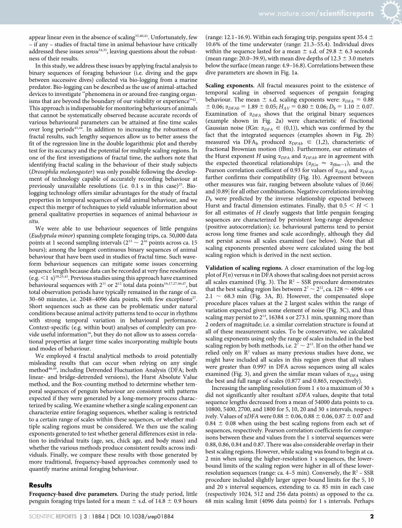
10.6% of the time underwater (range: 21.3–55.4). Individual diveswithin the sequence lasted for a mean 6 s.d. of 29.8 6 6.3 seconds(mean range: 20.0–39.9), with mean dive depths of 12.3 6 3.0 metersbelow the surface (mean range: 4.9–16.8). Correlations between thesedive parameters are shown in Fig. 1a.

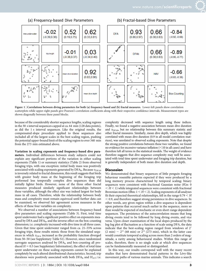
Scaling exponents. All fractal measures point to the existence oftemporal scaling in observed sequences of penguin foragingbehaviour. The mean 6 s.d. scaling exponents were: aDFA 5 0.886 0.06; aDFAb 5 1.89 6 0.05; HAV 5 0.80 6 0.06; Db 5 1.10 6 0.07.Examination of aDFA shows that the original binary sequences(example shown in Fig. 2a) were characteristic of fractionalGaussian noise (fGn: aDFA g (0,1)), which was confirmed by thefact that the integrated sequences (examples shown in Fig. 2b)measured via DFAb produced aDFAb g (1,2), characteristic offractional Brownian motion (fBm). Furthermore, our estimates ofthe Hurst exponent H using aDFA and aDFAb are in agreement withthe expected theoretical relationships (afGn < afBm21), and thePearson correlation coefficient of 0.93 for values of aDFA and aDFAb

further confirms their compatibility (Fig. 1b). Agreement betweenother measures was fair, ranging between absolute values of j0.66jand j0.89j for all other combinations. Negative correlations involvingDb were predicted by the inverse relationship expected betweenHurst and fractal dimension estimates. Finally, that 0.5 , H , 1for all estimates of H clearly suggests that little penguin foragingsequences are characterized by persistent long-range dependence(positive autocorrelation); i.e. behavioural patterns tend to persistacross long time frames and scale accordingly, although they didnot persist across all scales examined (see below). Note that allscaling exponents presented above were calculated using the bestscaling region which is derived in the next section.

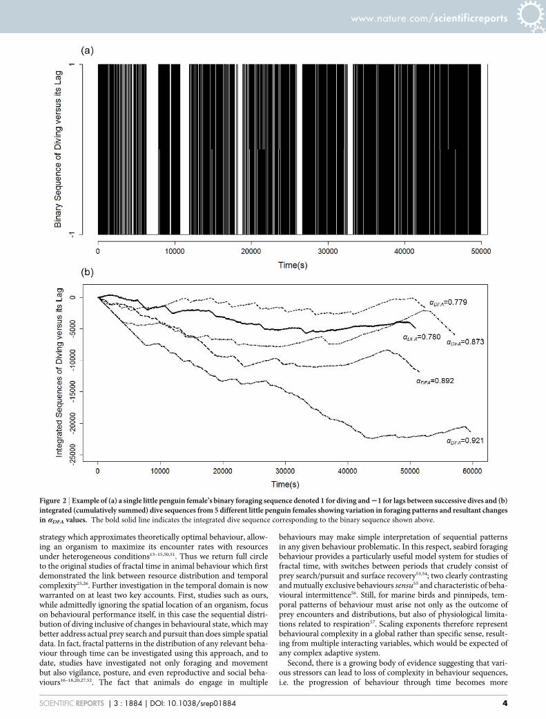
Validation of scaling regions. A closer examination of the log-logplot of F(n) versus n in DFA shows that scaling does not persist acrossall scales examined (Fig. 3). The R2 – SSR procedure demonstratesthat the best scaling region lies between 27 , 212, ca. 128 , 4096 s or2.1 , 68.3 min (Fig. 3A, B). However, the compensated slopeprocedure places values at the 2 largest scales within the range ofvariation expected given some element of noise (Fig. 3C), and thusscaling may persist to 214, 16384 s or 273.1 min, spanning more than2 orders of magnitude; i.e. a similar correlation structure is found atall of these measurement scales. To be conservative, we calculatedscaling exponents using only the range of scales included in the bestscaling region by both methods, i.e. 27 , 212. If on the other hand werelied only on R2 values as many previous studies have done, wemight have included all scales in this region given that all valueswere greater than 0.997 in DFA across sequences using all scalesexamined (Fig. 3), and given the similar mean values of aDFA usingthe best and full range of scales (0.877 and 0.865, respectively).

Increasing the sampling resolution from 1 s to a maximum of 30 sdid not significantly alter resultant aDFA values, despite that totalsequence lengths decreased from a mean of 54000 data points to ca.10800, 5400, 2700, and 1800 for 5, 10, 20 and 30 s intervals, respect-ively. Values of aDFA were 0.88 6 0.06, 0.88 6 0.06, 0.87 6 0.07 and0.84 6 0.08 when using the best scaling regions from each set ofsequences, respectively. Pearson correlation coefficients for compar-isons between these and values from the 1 s interval sequences were0.88, 0.86, 0.84 and 0.87. There was also considerable overlap in theirbest scaling regions. However, while scaling was found to begin at ca.2 min when using the higher-resolution 1 s sequences, the lower-bound limits of the scaling region were higher in all of these lower-resolution sequences (range: ca. 4–5 min). Conversely, the R2 – SSRprocedure included slightly larger upper-bound limits for the 5, 10and 20 s interval sequences, extending to ca. 85 min in each case(respectively 1024, 512 and 256 data points) as opposed to the ca.68 min scaling limit (4096 data points) for 1 s intervals. Perhaps

www.nature.com/scientificreports

SCIENTIFIC REPORTS | 3 : 1884 | DOI: 10.1038/srep01884 2

because of the considerably shorter sequence lengths, scaling regionsin the 30 s interval sequences capped at ca. 64 min (128 data points),as did the 1 s interval sequences. Like the original results, thecompensated-slope procedure applied to these sequences alsoincluded all of the largest scales in the best scaling region, pushingthe potential upper-bound limit of the scaling region to over 340 minfrom the 273 min estimated above.

Variation in scaling exponents and frequency-based dive para-meters. Individual differences between study subjects could notexplain any significant portions of the variation in either scalingexponents (Table 1) or summary statistics (Table 2) from observedforaging trips, with one exception: initial body mass was positivelyassociated with scaling exponents generated by DFAb. Because aDFAb

is inversely related to fractal dimension, this result suggests that birdswith greater body mass at the beginning of the foraging tripperformed less temporally complex dive sequences than didinitially lighter birds. However, none of the three other fractalmeasures produced similarly significant relationships betweenthese variables, although the effect size was indeed largest for bodymass in all cases. Therefore, while the relationship between bodymass and complexity must remain equivocal until further data canbe examined, we observed fair agreement across measures in theeffects of these four variables on complexity.

We observed a number of associations between frequency-baseddive parameters and scaling exponents (Table 3). First, total timespent underwater had a significant positive effect on exponents mea-sured by DFA and DFAb, and the inverse effect on the box-countingdimension; i.e. complexity increased with dive time in all three cases.Given that time spent underwater ranged from ca. 21–55% acrossforaging trips, these results mimic those from the simulated sequ-ences in which aDFA increased as the probability function divergedfrom 50–50 (see Supplentary Table S1). However, since randomizedsurrogate sequences analysed by DFAb and box-counting all pro-duced H 5 0.5 (see Supplentary Information), the effect of total timespent underwater on these scaling exponents cannot be explainedcompletely by such altered distributional characteristics. Second, tripdurations were positively associated with both DFAb and HAV; i.e.

complexity decreased with sequence length using these indices.Finally, we found a negative association between mean dive durationand aDFAb, but no relationship between this summary statistic andother fractal measures. Similarly, mean dive depth, which was highlycorrelated with mean dive duration (0.9 in all model correlation mat-rices), was unrelated to observed scaling exponents. Note that despitethe strong positive correlations between these two variables, we foundno evidence for excessive variance inflation (,10 in all cases) and havetherefore left all terms in the statistical models. The weight of evidencetherefore suggests that dive sequence complexity may well be assoc-iated with total time spent underwater and foraging trip duration, butis generally independent of both mean dive duration and depth.

DiscussionWe demonstrated that binary sequences of little penguin foragingbehaviour resemble patterns expected if they were produced by along memory process characterized by temporal scaling; binarysequences were consistent with fractional Gaussian noise (fGn: 0, H , 1) while integrated sequences were consistent with fractionalBrownian motion (fBm: 1 , H , 2). Scaling exponents of all analysesfit their expected theoretical relationships, fell in the range 0.79 , H, 0.9, and therefore suggest strong persistence in dive sequences. Inother words, any given region within a dive sequence is dependentupon patterns that occurred much earlier in the sequence, more sothan would be expected of stochastic or even short-range dependentsequences. The persistence of the autocorrelation means that longdiving events tend to be followed by long diving events, and viceversa. Upon closer examination of the local slopes produced by thelog-log plot of fluctuation as a function of scale using DFA, the dataindicate that the best-scaling region ranged from windows of 27

(2 min) , 212 (68 min) or 214 (273 min), which in the latter casewould constitute temporal scaling across more than 2 orders of mag-nitude, a rarity among behavioural studies. Within this range ofscales, therefore, there is no single scale at which dive sequencescan be fundamentally measured or distinguished.

In this way, our results correspond well with the many recentstudies that have demonstrated fractal patterns in the Levy-likemovement paths of various marine animals. This indicates a search

Figure 1 | Correlations between diving parameters for both (a) frequency-based and (b) fractal measures. Lower-left panels show correlation

scatterplots while upper-right panels give Pearson’s correlation coefficients along with their respective confidence intervals. Measurement types are

shown diagonally between these panel blocks.

www.nature.com/scientificreports

SCIENTIFIC REPORTS | 3 : 1884 | DOI: 10.1038/srep01884 3

strategy which approximates theoretically optimal behaviour, allow-ing an organism to maximize its encounter rates with resourcesunder heterogeneous conditions13–15,50,51. Thus we return full circleto the original studies of fractal time in animal behaviour which firstdemonstrated the link between resource distribution and temporalcomplexity25,26. Further investigation in the temporal domain is nowwarranted on at least two key accounts. First, studies such as ours,while admittedly ignoring the spatial location of an organism, focuson behavioural performance itself, in this case the sequential distri-bution of diving inclusive of changes in behavioural state, which maybetter address actual prey search and pursuit than does simple spatialdata. In fact, fractal patterns in the distribution of any relevant beha-viour through time can be investigated using this approach, and todate, studies have investigated not only foraging and movementbut also vigilance, posture, and even reproductive and social beha-viours16–18,20,27,52. The fact that animals do engage in multiple

behaviours may make simple interpretation of sequential patternsin any given behaviour problematic. In this respect, seabird foragingbehaviour provides a particularly useful model system for studies offractal time, with switches between periods that crudely consist ofprey search/pursuit and surface recovery53,54; two clearly contrastingand mutually exclusive behaviours sensu55 and characteristic of beha-vioural intermittence56. Still, for marine birds and pinnipeds, tem-poral patterns of behaviour must arise not only as the outcome ofprey encounters and distributions, but also of physiological limita-tions related to respiration57. Scaling exponents therefore representbehavioural complexity in a global rather than specific sense, result-ing from multiple interacting variables, which would be expected ofany complex adaptive system.

Second, there is a growing body of evidence suggesting that vari-ous stressors can lead to loss of complexity in behaviour sequences,i.e. the progression of behaviour through time becomes more

Figure 2 | Example of (a) a single little penguin female’s binary foraging sequence denoted 1 for diving and 21 for lags between successive dives and (b)integrated (cumulatively summed) dive sequences from 5 different little penguin females showing variation in foraging patterns and resultant changesin aDFA values. The bold solid line indicates the integrated dive sequence corresponding to the binary sequence shown above.

www.nature.com/scientificreports

SCIENTIFIC REPORTS | 3 : 1884 | DOI: 10.1038/srep01884 4

periodic or stereotypical. This also suggests that scaling exponentscan be used to characterize some aspect of individual or envir-onmental quality. A number of studies have tested this hypothesis,showing that impairments or challenges ranging from parasiticinfection through toxic substance exposure to increased exposureto anthropogenic disturbance16–21,27,58 are all associated with suchcomplexity loss16–19,21,58. This may have major implications concern-ing the viability of individuals operating in a sub-optimal state. It willbe interesting to determine whether similar examples of complexityloss can be demonstrated using spatial data collected from challengedindividuals. Although the animal movement ecology literature onstatistical patterns of search is growing with reference to optimality

and response to environmental cues, little attention has been paid tointrinsic factors that might cause variation in scaling across indivi-duals under the same ecological conditions55. Indeed, there seems tobe a divide in the current literature in which spatial patterns (animallocations through time) and temporal patterns (behavioural changesthrough time) are generally discussed in relation to extrinsic (e.g.landscape variables) and intrinsic (e.g. health states) control mechan-isms, respectively. Integration of these two domains and the frame-work through which their results are interpreted should therefore bea goal of future research, to further our understanding of how ani-mals respond to scales in both time and space, and to investigatewhether complexity loss is a feature of both.

Figure 3 | Validation of scaling regions in sequences of diving behaviour from little penguins. (A) The R2 – SSR procedure determines the

values of log(scale) that maximize the coefficient of determination and minimize the sum of squared residuals (*), corresponding to the range of scales

across which the data reflect strong scaling behaviour (filled circles shown in (B)). Note that when all scales are used (1) the coefficient of determination

remains comparable to that of the best scaling region, indeed all regression fits produced R2 values greater than 0.997, but the sum of squared residuals

increases dramatically. In this case, the estimates of aDFA for the best scaling region and the full range of scales are also comparable at 0.877 and 0.865,

respectively. (C) The compensated slope procedure allows testing the effect that varying the scaling exponent has on dispersion around a ‘‘zero-slope’’

(solid line), the point at which the scaling exponent is a true representation of the sequence. The scaling exponent derived from the best scaling region

produces values that best approximate a zero-slope (D), with all points examined falling within the 95% confidence intervals (dotted lines) generated by

1000 simulations of random variation around a zero-slope. Therefore, these observed sequences do exhibit fractal structure with power-law scaling

behaviour, i.e. strong linearity in the log-log plot of fluctuation as a function of scale, at least across the scales outlined in (B).

Table 1 | Results of linear mixed-effects models examining influence of individual traits on variation in scaling exponents from little penguinforaging sequences

Model Predictor est. s.e.m. df t Pr(. | t | )

DFA (Intercept) 0.652 0.168 13 3.884 0.002Age 20.001 0.002 10 20.604 0.560Sex (male) 20.046 0.027 10 21.677 0.125BM 0.0002 0.0001 10 1.750 0.111Chick Age 20.003 0.003 10 20.829 0.426

DFAb (Intercept) 1.611 0.145 13 11.124 0.000Age 0.000 0.002 10 20.188 0.855Sex (male) 20.040 0.023 10 21.730 0.114BM 0.0003 0.0001 10 2.238 0.049Chick Age 20.001 0.003 10 20.442 0.668

HAV (Intercept) 0.530 0.171 13 3.100 0.008Age 0.0001 0.002 10 0.026 0.979Sex (male) 20.037 0.028 10 21.302 0.222BM 0.0002 0.0001 10 1.588 0.143Chick Age 20.002 0.003 10 20.516 0.617

Box Count (Intercept) 1.354 0.163 13 8.320 0.000Age 20.001 0.002 10 20.374 0.716Sex (male) 0.030 0.027 10 1.120 0.289BM 20.0002 0.0001 10 21.615 0.137Chick Age 0.002 0.003 10 0.743 0.475

BM refers to initial body mass at time of logger deployment.

www.nature.com/scientificreports

SCIENTIFIC REPORTS | 3 : 1884 | DOI: 10.1038/srep01884 5

A key result of our study, however, is that scaling did not persistacross all scales examined, a common limitation of using thisapproach to characterize complete sequences. Indeed, this has beena major criticism of using fractal analysis in studies of animal beha-viour in the past59,60, although this criticism has been rebutted per-suasively34, largely because previous studies had not criticallyassessed the data upon which their scaling exponents were based.In the present study, the lack of clear scaling at smaller scales likelyreflects a combination of: (1) the influence of the mean individualdive durations, which were larger than most of these smaller scales at29.4 6 20.6 s; (2) decay of the strong short term autocorrelation; and,(3) mathematical error when small numbers of data points are usedin regression analyses. At the largest scales, it is impossible to deter-mine whether the bias in scaling is due to its absence or simply thepaucity of available windows, i.e. an artefact of finite sequence length.This can only be answered by collecting sequences of greater length,

which should continue to be a goal in future studies. What is prom-ising, however, is that changing the resolution of the data did not leadto significant changes in the fractal properties of observed sequences,although our results do suggest that higher- and lower-resolutionsequences may be better at detecting the presence of scaling at smalland large scales, respectively.

In addition to these measurement-related issues, there may bebiological reasons to expect changes in the correlation structure offoraging sequences at certain scales. This may in part reflect certainhabitat characteristics and how animals interact with their environ-ments at different scales. For example, the tortuosity of foragingpaths in wandering albatross (Diomedea exulans) differs across threescaling regions: patterns at the smallest scales (,100 m) reflectadjustment to wind currents, at medium scales (1–10 km) food-search behaviour, and at the largest scales (.10 km) long-distance movement between patches and change in local weather

Table 2 | Results of linear mixed-effects models examining influence of individual traits on variation in frequency-based dive parametersfrom little penguin foraging sequences

Model Predictor est. s.e.m. df t Pr(. | t | )

Dive (Intercept) 52915.520 7613.679 13 6.950 0.000Trip Age 46.980 91.300 10 0.515 0.618Duration Sex (male) 2980.990 1264.637 10 20.776 0.456

BM 1.400 6.408 10 0.219 0.831Chick Age 299.560 138.918 10 20.717 0.490

Dive (Intercept) 36.188 18.474 13 1.959 0.072Duration Age 0.195 0.227 10 0.861 0.409

Sex (male) 0.793 2.962 10 0.268 0.794BM 20.009 0.015 10 20.592 0.567Chick Age 0.249 0.334 10 0.746 0.473

Dive (Intercept) 16.067 9.085 13 1.768 0.100Depth Age 0.022 0.111 10 0.202 0.844

Sex (male) 0.618 1.459 10 0.424 0.681BM 20.005 0.008 10 20.651 0.530Chick Age 0.184 0.164 10 1.124 0.287

Underwater (Intercept) 0.482 0.228 13 2.111 0.055Time Age 20.001 0.003 10 20.348 0.735

Sex (male) 0.054 0.038 10 1.413 0.188BM 20.0002 0.0002 10 20.783 0.452Chick Age 0.005 0.004 10 1.244 0.242

BM refers to initial body mass at time of logger deployment.

Table 3 | Results of linear mixed-effects models examining relationship between scaling exponents and frequency-based dive parametersfrom little penguin foraging sequences

Model Predictor est. s.e.m. df t Pr(. | t | )

DFA (Intercept) 0.796 0.156 13 5.093 0.000Trip Duration 5.2E-06 2.8E-06 10 1.865 0.092Underwater Time 20.396 0.111 10 23.568 0.005Dive Duration 0.003 0.003 10 0.830 0.426Dive Depth 20.010 0.007 10 21.482 0.169

DFAb (Intercept) 1.810 0.104 13 17.480 0.000Trip Duration 5.0E-06 1.8E-06 10 2.716 0.022Underwater Time 20.357 0.073 10 24.921 0.001Dive Duration 0.003 0.002 10 1.250 0.240Dive Depth 20.011 0.005 10 22.331 0.042

HAV (Intercept) 0.299 0.200 13 1.491 0.160Trip Duration 1.1E-05 3.6E-06 10 2.994 0.014Underwater Time 0.016 0.145 10 0.109 0.915Dive Duration 0.002 0.004 10 0.486 0.638Dive Depth 20.014 0.009 10 21.597 0.141

Box Count (Intercept) 1.099 0.125 13 8.787 0.000Trip Duration 3.9E-06 2.3E-06 10 21.736 0.113Underwater Time 0.471 0.095 10 4.974 0.001Dive Duration 3.0E-04 2.4E-03 10 0.126 0.902Dive Depth 0.004 0.005 10 0.821 0.431

www.nature.com/scientificreports

SCIENTIFIC REPORTS | 3 : 1884 | DOI: 10.1038/srep01884 6

conditions61. For central place foragers like the penguins studiedhere, travel between foraging sites and the colony, which can consti-tute a considerable portion of the total sequence length (trip dura-tion), may lead to scaling breaks at large scales. However, this cannotexplain the deviation from scaling we observed at large scales becauseour sequences began only when the first instances of diving wereobserved, eliminating any effects of such movement types.Landscape heterogeneity can also affect scaling in animal move-ments, such as in American martens (Martes americana) wheremovement paths are determined by microhabitat features at small(,3.5 meters) but not larger scales38, and in grazing ewes where suchfeatures affected movements at scales greater than a threshold value(5 meters)39. While addressing variation in microhabitat structure isbeyond the scope of the current study, prey locations are likely tohave contributed strongly to deviations from scaling at small scales.This would be compounded in seabirds by the necessary pauses inforaging as animals return to the surface to breathe57. Strong short-term autocorrelation can result from bouts in which animals dive tosimilar depths in pursuit of prey within a patch and then surface toreplenish oxygen reserves before repeating the process62.

In addition to the distinction between real and perceived scalingbreaks, another difficulty in inferring fractal structure is that it isgenerally always possible to find a short-range correlated model ofhigher order and complexity to fit any sequence with finite length33;i.e. all real world data. For example, DFA failed to distinguishbetween a real long-range dependent process and a short-rangeone generated by the super-position of three first-order autoregres-sive processes32. In real-world data, simple autoregressive modelshave been used to predict the correlation structure of sequential divedepths in macaroni penguins (Eudyptes chrysolophus) with someprecision63. However, other recent evidence also using successivemeasurements of dive depths strongly suggests that such sequencesare rather consistent with long memory processes in most cases15,50,51.Indeed, short-range correlations cannot adequately model many bio-logical and physical phenomena found in nature, which is why moreparsimonious models of long-range dependence were developed33.Our study is among the first to examine binary time series of animalbehaviour with lengths up to 216, sequences spanning 4 orders ofmagnitude and thus nearing and in some cases even exceeding thoseused in many simulation studies. Therefore, our results offer com-pelling support for long-range fractal structure in penguin divesequences.

Ultimately, while describing the scaling exponents of behaviouralsequences accurately is a fundamental component of this research,what may be of more interest to many researchers is the next step; theability to apply such quantifiable properties in distinguishingbetween the behaviours of various groups of individuals or taxa. Inthis regard, our study did not show any clear differences in thecomplexity signatures of individuals in relation to age, sex, or chickage, and produced only weak evidence for an effect of initial bodymass. Similarly, these variables also did not affect any of the summarystatistics measured. There is considerable variation across studies inthe impacts of such biological factors on seabird behaviour64–67, so itremains difficult to make any strong inferences based on as small adata set as that used here. However, it is clear that certain aspects offoraging behaviour such as time spent underwater and trip durationcan be correlated with dive sequence complexity. Our simulated datashow that DFA can be sensitive to variation in the probability dis-tribution of dives, but further analysis of the scaling region easilydistinguished between simulated and observed behaviour (seeSupplementary Information). Furthermore, reshuffling the divesproduced random sequences in 3 of our 4 fractal methods, all ofwhich correlated well with DFA, particularly DFAb. Together, theseresults suggest that time spent underwater and trip duration cannoton their own explain the variation in fractal scaling observed. It is alsonotable that neither mean dive duration nor depth was related to a

sequence’s fractal properties. Therefore, the sequential distributionof dives within a sequence is ultimately the key factor, adding weightto our assertion that temporal fractal analyses provide a metric thatdescribes a fundamental property in animal behaviour: fractal time26.

In conclusion, we show here that penguin dive sequences exhibit acomplex fractal structure through time, and relate this structure to acombination of extrinsic (environmental) and intrinsic (self) organ-izational control elements. The application of fractal tools to tem-poral sequences of animal behaviour should be explored further,particularly in, though far from limited to, organisms that are oftenused as indicator species for climate and environmental change, likethe penguins examined here and many other top predators in marineecosystems. The merger of bio-logging and fractal analysis representsan important opportunity to do so, promising to advance our under-standing of the many interactions that occur between animals andthe environments in which they are found.

MethodsStudy site & subjects. This study was conducted during the guard stage of the 2010breeding period (October 26 – November 26) with free-living little penguins(Eudyptula minor) at the Penguin Parade, Phillip Island (38u319S, 145u099E),Victoria, Australia. Birds from this colony were marked with injected passive RFIDtransponders (Allflex, Australia) as chicks68. We collected diving data consisting ofsingle full-day foraging trips from 28 penguins, 14 males and 14 females, guarding 1-to 2-week-old chicks. Each penguin’s age was determined from the date oftransponder injection. Sex was determined using bill depth measurements69. Wecaptured the birds in artificial wooden burrows and fitted them with time-depth dataloggers (ORI400-D3GT, Little Leonardo, 12 3 45 mm, 9 g) set to record depth to aresolution of 0.1 m with an accuracy of 1 m (range: 0–400 m) at one-secondintervals. Devices were attached using waterproof TesaH tape (Beiersdorf AG,Hamburg, Germany) along the median line of the lower back feathers to minimizedrag70 and facilitate rapid deployment and easy removal upon recapture71. After asingle foraging trip, each bird was recaptured in its nest box and the logger and tapewere removed. All birds were weighed before and after logger attachment. Fieldworkwas approved by the Phillip Island Animal Experimentation Ethics Committee(2.2010) and the Department of Sustainability and Environment of Victoria,Australia (number 10006148).

Frequency-based dive parameters. We first characterized dive sequences duringeach foraging trip with commonly-used summary statistics, including: (1) trip length;(2) mean dive duration; (3) mean dive depth; and, (4) total dive time, i.e. total timespent below the surface during a trip. After recovery, data were downloaded from theloggers and analysed using custom-written programs in IGOR Pro, version 6.22A(Wavemetrics, Portland, Oregon). We consider diving to have occurred only whenthe depth at a given sampling interval was greater than 1 m. We include Pearsoncorrelation tests to examine relationships between these parameters.

Fractal analyses. We applied 4 methods to estimate the scaling behaviour of observeddive sequences. We emphasize Detrended Fluctuation Analysis or DFA2 because ithas become a mainstream method for examining scaling behaviour in time series dataand remains the only method used to examine binary sequences of animal behaviour,though it is not without its critics72. For comparison, we used two variants of DFA (seebelow), but also two other measures in the Hurst Absolute Value (HAV) method73,74

and the box-counting method75. We performed DFA and HAV using the package‘fractal’76, and box-counting with the package ‘fractaldim’77, in R statistical softwarev.2.15.078.

Signal class. A critical first step in examining fractal structure in any data set forwhich the signal class is not a priori known is to determine whether the sequencesreflect fractional Gaussian noise (fGn) or fractional Brownian motion (fBm).Choosing an appropriate scaling exponent estimator and correctly interpreting theresults require knowledge about the class of the original signal30,31,41. We thereforetested the signal class of these sequences to determine whether they reflect fGn or fBmby examining the scaling exponent calculated by DFA (aDFA), with aDFA g (0,1)indicating fGn and aDFA g (1,2) indicating fBm.

Detrended fluctuation analysis (DFA). DFA is a robust method used to estimate theHurst exponent79,80, i.e. the degree to which time series are long-range dependent andself-affine30,73. The method is described in9, and its application to binary sequences ofanimal behaviour can be found in16,18,27. Other names for this method include lineardetrended scaled windowed variance30 and residuals of regression73. The followingdescription of DFA is taken from the above studies.

First, we coded dive sequences as binary time series [z(i)] in wave form containingdiving (denoted by 1) and lags between diving events (denoted by 21) at 1 s intervalsto length N. Diving behaviour was recorded at all t during which the subject wassubmerged to a depth greater than 1 m. Series were then integrated (cumulativelysummed) such that

www.nature.com/scientificreports

SCIENTIFIC REPORTS | 3 : 1884 | DOI: 10.1038/srep01884 7

y tð Þ~Xt

i~1

z ið Þ

where y(t) is the integrated time series.After integration, sequences were divided into non-overlapping boxes of length n, a

least-squares regression line was fit to the data in each box to remove local lineartrends (yn(t)), and this process was repeated over all box sizes such that

F nð Þ~

ffiffiffiffiffiffiffiffiffiffiffiffiffiffiffiffiffiffiffiffiffiffiffiffiffiffiffiffiffiffiffiffiffiffiffiffiffiffiffiffiffiffiffi1N

XN

i~1

yn tð Þ{yn tð Þ� �2

vuut

where F(n) is the average fluctuation of the modified root-mean-square equationacross all scales (22, 23, … 2n). The relationship between F and n is of the form

F nð Þ*na

where a is the slope of the line on a double logarithmic plot of average fluctuation as afunction of scale. Like all estimators of the Hurst exponent, aDFA 5 0.5 indicates anon-correlated, random sequence (white noise), aDFA ,0.5 indicates negative auto-correlation (anti-persistent long-range dependence), and aDFA .0.5 indicates pos-itive autocorrelation (persistent long-range dependence)9. Theoretically, aDFA isinversely related to the fractal dimension, a classical index of structural complexity81,and thus smaller values reflect greater complexity (see Theoretical Relationshipsbetween Scaling Exponents below).

In addition to the standard (linear) form of DFA, we also used a bridge detrendingmethod in our analysis, which is reportedly more appropriate to fBm signals49 andsequences of lengths greater than 21230. Bridge-detrended Fluctuation Analysis(hereafter DFAb) differs in two distinct ways from the linear form. Bridge-detrendedFluctuation Analysis (hereafter DFAb) differs in two distinct ways from the linearform. First, rather than using the regression line that best fits all data points in eachwindow to detrend the sequence, the slope of the line bridging only the first and lastpoints in each window is calculated30. Second, since it was suggested to work well withfBm rather than fGn sequences49, and assuming that original binary sequences in thisstudy were of the class fGn, we first integrated our time series before applying DFAb,meaning that observed sequences were integrated twice during application of DFAbbut only once during DFA. We refer to the scaling exponent generated by this analysisas aDFAb.

Hurst absolute value method (HAV). We calculated the Hurst exponent H directlyusing the Absolute Value method. While fractal dimension estimates theoreticallyprovide information about both memory and self-similarity or self-affinity, aprevious study has shown that DFA, while giving robust estimates of long-rangedependence (serial correlation), fails to capture the self-similarity parameter in datawith certain non-Gaussian distributional characteristics74. The same study showedthat the absolute value method, on the other hand, captured both parameters. Usingthis method, time series of length N are divided into smaller windows of length m andthe first absolute moment is calculated as

d mð Þ~1

N=m

XN=m

k~1

X mð Þ kð Þ{ Xh i�� ��

where X(m) is a window of length m and ÆXæ is the mean of the entire series. Thevariance d scales with the window size m as

d mð Þ~mHAV{1

where HAV is the scaling (absolute value) exponent. Note that while DFA firstintegrates the time series before calculation, HAV is calculated from the original timeseries, which in this case is the binary sequence of dives and their lags.

Box-counting dimension. We also employ a classical measure of fractal dimension tomeasure sequence complexity; box-counting75,82. The principle behind box-countingis simple. First, the integrated curve of the time series is placed within a single box,which is subsequently divided into smaller and smaller equally-sized boxes of size n.We use the entire range of scales from total sequence length down to the resolution ofthe data (i.e. 1 s). At each value of n, the number of boxes required to cover the curve iscounted, with the expected relationship

N nð Þ~kn{Db

where n is the box size, N(n) represents the number of boxes required to cover thecurve at each box size, k is a constant, and Db is the box-counting dimension, which isestimated from the slope of the least squares regression line on the log-log plot of N(n)as a function of n.

Validation of scaling region. We use various methods to ensure the validity of ourDFA results. There are algorithmic reasons why values diverge from scaling at smalland large scales in a given analysis, and some of these are specific to the method used.For example, omitting some of the smallest and largest scales from the analysis isrecommended when using DFA and DFAb; excluding the largest scales can reducevariance but increase bias, whereas excluding the smallest scales reduces bias but

increases variance30. The range of scales used should therefore be selected to maximizethe fit of the regression line, i.e. minimize the mean squared error, on the doublelogarithmic plot30. Similarly, excluding scales smaller than 1/5 of the total sequencelength as well as the two largest scales is recommend when using box-counting75.Alternatively, multiple scaling regions may also exist for biological reasons as aresponse of an organism to temporal or spatial scale34,36–38. Therefore, weindependently determined the appropriate range(s) of scales within which strongscaling behaviour existed in our observed sequences using two procedures describedin detail in35.

The R2 – SSR procedure involves the creation of a series of regression windows inwhich the number of data points (scales) ranges from a minimum of 5 (for validregression analysis) to the maximum number of scales examined, 14 in our case. Eachwindow was then slid across the entire data set so that the smallest windows provided8 regression estimates, the next window size 7, and so on until only a single regressionwas performed on the largest window covering all scales. For fractal sequences, thereshould be a point at which, on a plot of the coefficient of variation (R2) versus the sumof squared residuals (SSR), points converge to maximize the former and minimize thelatter. This allows for the identification of the best scaling regions to be used in thecalculation of scaling exponents in observed sequences. We performed this analysison the mean values of F(n) and n across all observed sequences, and therefore do nottest for variation in scaling regions across individual birds.

The compensated-slope procedure uses a scaling factor c to ‘compensate’ thescaling behaviour such that, in the case of DFA,

F nð Þ~nc � n{Df

where F(n) is the fluctuation about the box size n as described above, c is the com-pensation exponent taking values of c g (0, 1) for self-affine curves such as thoseexamined here, and Df is the fractal dimension estimate for the sequence. By varying cbetween 0 and 1, we can find the value at which our dimension estimate (based on therange of scales determined via the R2 – SSR procedure) and compensated slopeconverge to 0 to produce a straight line (if scaling exists) with slope zero on the plot ofLog(nc*n2Df) versus Log(n). Here, we used 5 values for c, the lowest (0.70) and highest(1.00) of which for illustrative purposes and the middle three values representing theminimum, best, and maximum estimates of aDFA derived from the sliding windowsused in the R2 – SSR procedure. We then bootstrapped 1000 simulations to determinewhether variation from this zero slope in observed sequences could be explained bynoise, i.e. data points fall within the 95% confidence intervals, or whether scaling wassimply unlikely given the fractal dimension estimate produced.

While the procedures described above are robust, many previous studies haverelied on less convincing measures to support their results, such as high coefficients ofvariation for the slope of the double logarithmic plot and showing that surrogatesequences in which observed data points have been shuffled to break any serialcorrelation results in the expected relationship aDFArandom 5 0.516,27,46. We also pre-sent R2 values in our study, and take the mean of 10 surrogate sequences for eachobserved sequence (i.e. N 5 28*10 5 280), but additionally apply the R2 – SSR andcompensated-slope procedures to these randomized sequences for comparison withobserved sequences. Furthermore, we computed aDFA for simulated random binarysequences of various lengths (211 , 216 s) and distributions of diving behaviour (100simulations for each of 5 binary probability distributions, i.e. diving versus its lag, at0.25, 0.33, 0.50, 0.66, and 0.75) for comparison with observed and surrogate data. Theresults of these analyses are presented as Supplementary Information online.

Finally, in addition to the original 1 s interval sequences, we also applied the linearform of DFA to sequences sampled at 5, 10, 20 and 30 s intervals to determinewhether the same scaling relationship would hold given different data resolutions. Wealso applied the R2 – SSR and compensated-slope procedures to these sequences todetermine whether their scaling regions corresponded to those in the high-resolution1 s interval sequences.

Theoretical relationships between scaling exponents. Most scaling exponents andother fractal dimension estimates are theoretically related. For example, aDFA

provides a robust estimate of the Hurst exponent H30,73, such thatfor fGn: H 5 aDFA

for fBm: H 5 aDFA 2 1In addition, H itself is inversely related to fractal dimension, here the box-counting

dimension, such that for one-dimensional time series like those examined here

Df ~2{H

While these measures are theoretically related, in practice the various methodsoften lead to different results, either because of mathematical differences or non-linearity in the series themselves73,83,84. Therefore, we estimated each of these para-meters separately using the methods described above for a more robust interpretationof the results. We include an analysis of Pearson correlation coefficients to test foragreement between the four measures used.

Statistical analyses. Using the scaling exponents estimated via the above methods asGaussian-distributed response variables (X2 goodness-of-fit tests, P.0.05), weconstructed general linear mixed-effects (LME) models to determine whether age,sex, initial body mass and the age of the young chicks being guarded were associatedwith variation in penguin dive sequence complexity (N 5 28). We could not use finalbody mass to calculate mass gain during trips because measurements were takenhours after birds had returned to the nest and had already fed their chicks. We used

www.nature.com/scientificreports

SCIENTIFIC REPORTS | 3 : 1884 | DOI: 10.1038/srep01884 8

the same approach to test whether these individual factors could explain varianceobserved in the summary statistics for each foraging trip, which were also Gaussian-distributed across individuals (X2 goodness-of-fit tests, P.0.05). For all models, weset the date on which data were collected for each individual as a random factor in ouranalyses to control for temporal variation. All LME models were run using the nlmepackage85 in R. Models were fit by restricted maximum likelihood, using all factorsand covariates in a single full model to estimate the parameter effects. Finally, we useda general linear model (GLM) to test whether the summary statistics themselves couldexplain variation in the observed scaling exponents. In all models, we tested forvariance inflation caused by correlation between fixed effects using the car package inR86. If the variance inflation factor exceeded 10, we arbitrarily removed one of the 2correlated variables and ran the model again. We set the alpha level for all statisticalanalyses at 0.05.

1. Havlin, S. et al. Scaling in nature: from DNA through heartbeats to weather.Physica A -Statistical Mechanics and Its Applications 273, 46–69 (1999).

2. Peng, C. K. et al. Long-range correlations in nucleotide sequences. Nature 356,168–170 (1992).

3. Stanley, H. E. et al. Scaling and universality in animate and inanimate systems.Physica A -Statistical Mechanics and Its Applications 231, 20–48 (1996).

4. Goldberger, A. L., Rigney, D. R. & West, B. J. Chaos and fractals in humanphysiology. Sci. Am. 262, 43–49 (1990).

5. Peng, C. K. et al. Quantifying fractal dynamics of human respiration: age andgender effects. Ann. Biomed. Eng. 30, 683–692 (2002).

6. West, B. J. & Goldberger, A. L. Physiology in fractal dimensions. Am. Sci. 75,354–365 (1987).

7. Mandelbrot, B. B. How long is the coast of Britain? Statistical self-similarity andfractional dimension. Science 156, 636–638 (1967).

8. Glenny, R. W., Robertson, H. T., Yamashiro, S. & Bassingthwaighte, J. B.Applications of fractal analysis to physiology. J. Appl. Physiol. 70, 2351–2367(1991).

9. Peng, C. K., Havlin, S., Stanley, H. E. & Goldberger, A. L. Quantification of scalingexponents and crossover phenomena in nonstationary heartbeat time-series.Chaos 5, 82–87 (1995).

10. Nelson, T. R., West, B. J. & Goldberger, A. L. The fractal lung: universal andspecies-related scaling patterns. Experientia 46, 251–254 (1990).

11. Shlesinger, M. F. & West, B. J. Complex fractal dimension of the bronchial tree.Phys. Rev. Lett. 67, 2106–2108 (1991).

12. Viswanathan, G. M., Da Luz, M. G. E., Raposo, E. P. & Stanley, H. E. The physics offoraging. (Cambridge University Press, 2011).

13. Bartumeus, F. Levy processes in animal movement: an evolutionary hypothesis.Fractals 15, 151–162 (2007).

14. Viswanathan, G. M., Raposo, E. P. & da Luz, M. G. E. Levy flights andsuperdiffusion in the context of biological encounters and random searches.Physics of Life Reviews 5, 133–150 (2008).

15. Sims, D. W. et al. Scaling laws of marine predator search behaviour. Nature 451,1098–1102 (2008).

16. MacIntosh, A. J., Alados, C. L. & Huffman, M. A. Fractal analysis of behaviour in awild primate: behavioural complexity in health and disease. J. Royal Soc. Interface8, 1497–1509 (2011).

17. Alados, C. L., Escos, J. M. & Emlen, J. M. Fractal structure of sequential behaviourpatterns: an indicator of stress. Anim. Behav. 51, 437–443 (1996).

18. Alados, C. L. & Weber, D. N. Lead effects on the predictability of reproductivebehavior in fathead minnows (Pimephales promelas): a mathematical model.Environ. Toxicol. Chem. 18, 2392–2399 (1999).

19. Motohashi, Y., Miyazaki, Y. & Takano, T. Assessment of behavioral effects oftetrachloroethylene using a set of time series analyses. Neurotoxicol. Teratol. 15,3–10 (1993).

20. Rutherford, K. M. D., Haskell, M. J., Glasbey, C. & Lawrence, A. B. The responsesof growing pigs to a chronic-intermittent stress treatment. Physiol. Behav. 89,670–680 (2006).

21. Seuront, L. & Cribb, N. Fractal analysis reveals pernicious stress levels related toboat presence and type in the Indo-Pacific bottlenose dolphin, Tursiops aduncus.Physica A -Statistical Mechanics and Its Applications 390, 2333–2339 (2011).

22. West, B. J. Physiology in fractal dimensions: error tolerance. Ann. Biomed. Eng.18, 135–149 (1990).

23. Goldberger, A. L. Fractal variability versus pathologic periodicity: complexity lossand stereotypy in disease. Perspect. Biol. Med. 40, 543–561 (1997).

24. Shimada, I., Kawazoe, Y. & Hara, H. A temporal model of animal behavior basedon a fractality in the feeding of Drosophila melanogaster. Biol. Cybern. 68, 477–481(1993).

25. Shimada, I., Minesaki, Y. & Hara, H. Temporal fractal in the feeding behavior ofDrosophila melanogaster. J. Ethol. 13, 153–158 (1995).

26. Cole, B. J. Fractal time in animal behavior: the movement activity of Drosophila.Anim. Behav. 50, 1317–1324 (1995).

27. Alados, C. L. & Huffman, M. A. Fractal long-range correlations in behaviouralsequences of wild chimpanzees: a non-invasive analytical tool for the evaluation ofhealth. Ethology 106, 105–116 (2000).

28. Delignieres, D. et al. Fractal analyses for ‘short’ time series: A re-assessment ofclassical methods. J. Math. Psychol. 50, 525–544 (2006).

29. Weron, R. Estimating long-range dependence: finite sample properties andconfidence intervals. Physica A -Statistical Mechanics and Its Applications 312,285–299 (2002).

30. Cannon, M. J., Percival, D. B., Caccia, D. C., Raymond, G. M. & Bassingthwaighte,J. B. Evaluating scaled windowed variance methods for estimating the Hurstcoefficient of time series. Physica A: Statistical Mechanics and its Applications241, 606–626 (1997).

31. Eke, A. et al. Physiological time series: distinguishing fractal noises from motions.Pflugers Archiv-European Journal of Physiology 439, 403–415 (2000).

32. Maraun, D., Rust, H. W. & Timmer, J. Tempting long-memory - on theinterpretation of DFA results. Nonlinear Processes in Geophysics 11, 495–503(2004).

33. Beran, J. Statistics for long-memory processes. (Chapman and Hall/CRC, 1994).34. Seuront, L., Brewer, M. & Strickler, J. R. in Handbook of scaling methods in aquatic

ecology (eds Seuront, L. & Strutton, P. G.) 333–359 (CRC Press, 2004).35. Seuront, L. Fractals and multifractals in ecology and aquatic science. 344 (Taylor

and Francis, LLC, 2010).36. Wiens, J. A., Crist, T. O., With, K. A. & Milne, B. T. Fractal patterns of insect

movement in microlandscape mosaics. Ecology 76, 663–666 (1995).37. Nams, V. O. Using animal movement paths to measure response to spatial scale.

Oecologia 143, 179–188 (2005).38. Nams, V. O. & Bourgeois, M. Fractal analysis measures habitat use at different

spatial scales: an example with American marten. Can. J. Zool. 82, 1738–1747(2005).

39. Garcia, F., Carrere, P., Soussana, J. F. & Baumont, R. Characterisation by fractalanalysis of foraging paths of ewes grazing heterogeneous swards. Appl. Anim.Behav. Sci. 93, 19–37 (2005).

40. Clauset, A., Shalizi, C. & Newman, M. Power-Law Distributions in EmpiricalData. SIAM Review 51, 661–703 (2009).

41. Delignieres, D., Torre, K. & Lemoine, L. Methodological issues in the applicationof monofractal analyses in psychological and behavioral research. NonlineraDynamics, Psychology, and Life Sciences 9, 451–477 (2005).

42. Boyd, I. L., Kato, A. & Ropert-Coudert, Y. Bio-logging science: sensing beyond theboundaries. Memoirs of the National Institute of Polar Research 58, 1–14 (2004).

43. Ropert-Coudert, Y. & Wilson, R. P. Trends and perspectives in animal-attachedremote sensing. Frontiers in Ecology and the Environment 3, 437–444 (2005).

44. Ropert-Coudert, Y., Kato, A., Gremillet, D. & Crenner, F. in Sensors for Ecology:Towards integrated knowledge of ecosystems (eds Le Galliard, J. F., Guarini, J. M. &Gaill, F.) 17–41 (Centre National de la Recherche Scientifique (CNRS), InstitutEcologie et Environnement (INEE) 2012).

45. Kembro, J. M., Marin, R. H., Zygaldo, J. A. & Gleiser, R. M. Effects of the essentialoils of Lippia turbinata and Lippia polystacha (Verbenaceae) on the temporalpattern of locomotion of the mosquito Culex quinquefasciatus (Diptera:Culicidae) larvae. Parasitol. Res. 104, 1119–1127 (2009).

46. Kembro, J. M., Perillo, M. A., Pury, P. A., Satterlee, D. G. & Marin, R. H. Fractalanalysis of the ambulation pattern of Japanese quail. Br. Poult. Sci. 50, 161–170(2009).

47. Rutherford, K. M. D., Haskell, M. J., Glasbey, C., Jones, R. B. & Lawrence, A. B.Fractal analysis of animal behaviour as an indicator of animal welfare. Anim. Welf.13, S99–S103 (2004).

48. Gao, J. B. et al. Assessment of long-range correlation in time series: How to avoidpitfalls. Physical Review E 73, (2006).

49. Stroe-Kunold, E., Stadnytska, T., Werner, J. & Braun, S. Estimating long-rangedependence in time series: An evaluation of estimators implemented in R. Behav.Res. Methods 41, 909–923 (2009).

50. Humphries, N. E. et al. Environmental context explains Levy and Brownianmovement patterns of marine predators. Nature 465, 1066–1069 (2010).

51. Sims, D. W., Humphries, N. E., Bradford, R. W. & Bruce, B. D. Levy flight andBrownian search patterns of a free-ranging predator reflect different prey fieldcharacteristics. J. Anim. Ecol. 81, 432–442 (2012).

52. Rutherford, K. M. D., Haskell, M. J., Glasbey, C., Jones, R. B. & Lawrence, A. B.Detrended fluctuation analysis of behavioural responses to mild acute stressors indomestic hens. Appl. Anim. Behav. Sci. 83, 125–139 (2003).

53. Houston, A. I. & Carbone, C. The optimal llocation of time during the dive cycle.Behav. Ecol. 3, 233–262 (1992).

54. Kooyman, G. L. Diverse divers: physiology and behavior. (Springer-Verlag, 1989).55. Reynolds, A. M. On the origin of bursts and heavy tails in animal dynamics.

Physica A -Statistical Mechanics and Its Applications 390, 245–249 (2011).56. Bartumeus, F. Behavioral intermittence, Levy patterns, and randomness in animal

movement. Oikos 118, 488–494 (2009).57. Kramer, D. L. Thebehavioral ecology of air breathing by aquatic animals. Can. J.

Zool. 66, 89–94 (1988).58. Seuront, L. & Leterme, S. Increased zooplankton behavioral stress in response to

short-term exposure to hydrocarbon contamination. The Open OceanographyJournal 1, 1–7 (2007).

59. Turchin, P. Fractal analyses of animal movement: A Critique. Ecology 77,2086–2090 (1996).

60. Benhamou, S. How to reliably estimate the tortuosity of an animal’s path::straightness, sinuosity, or fractal dimension? J. Theor. Biol. 229, 209–220 (2004).

61. Fritz, H., Said, S. & Weimerskirch, H. Scale–dependent hierarchical adjustmentsof movement patterns in a long–range foraging seabird. Proc. R. Soc. Lond. B Biol.Sci. 270, (2003).

www.nature.com/scientificreports

SCIENTIFIC REPORTS | 3 : 1884 | DOI: 10.1038/srep01884 9

62. Mori, Y. Dive bout organization in the chinstrap penguin at seal island, Antarctica.J. Ethol. 15, 9–15 (1997).

63. Hart, T., Coulson, T. & Trathan, P. N. Time series analysis of biologging data:autocorrelation reveals periodicity of diving behaviour in macaroni penguins.Anim. Behav. 79, 845–855 (2010).

64. Ropert-Coudert, Y., Kato, A., Naito, Y. & Cannell, B. L. Individual divingstrategies in the Little Penguin. Waterbirds 26, 403–408 (2003).

65. Le Vaillant, M. et al. How age and sex drive the foraging behaviour in the kingpenguin. Marine Biology 160, 1147–1156 (2013).

66. Kato, A., Ropert-Coudert, Y. & Chiaradia, A. Regulation of trip duration by aninshore forager, the little penguin (Eudyptula Minor), during incubation. The Auk125, 588–593 (2008).

67. Zimmer, I., Ropert-Coudert, Y., Poulin, N., Kato, A. & Chiaradia, A. Evaluatingthe relative importance of intrinsic and extrinsic factors on the foraging activity oftop predators: a case study on female little penguins. Marine Biology 158, 715–722(2011).

68. Chiaradia, A. & Kerry, K. R. Daily nest attendance and breeding performance inthe Little Penguin Eudyptula minor at Phillip Island, Australia. Mar. Ornithol. 27,13–20 (1999).

69. Arnould, J. P., Dann, P. & Cullen, J. M. Determining the sex of little penguins(Eudyptula minor) in northern Bass Strait using morphometric measurements.Emu 104, 261–265 (2004).

70. Bannasch, D. G., Wilson, R. P. & Culik, B. Hydrodynamic aspects of design andattachment of a back-mounted device in penguins. J. Theor. Biol. 194, 83–96(1994).

71. Wilson, R. P. et al. Long term attachment of transmitting and recording devices topenguins and other seabirds. Wildl. Soc. Bull. 25, 101–106 (1997).

72. Bryce, R. M. & Sprague, K. B. Revisiting detrended fluctuation analysis. Sci. Rep. 2(2012).

73. Taqqu, M. S., Teverovsky, V. & Willinger, W. Estimators for long-rangedependence: an empirical study. Fractals 3, 785–788 (1995).

74. Mercik, S., Weron, K., Burnecki, K. & Weron, A. Enigma of self-similarity offractional Levy stable motions. Acta Physica Polonica B 34, 3773–3791 (2003).

75. Liebovitch, L. S. & Toth, T. A fast algorithm to determine fractal dimensions bybox counting. Phys. Lett. A 141, 386–390 (1989).

76. Constantine, W. & Percival, D. fractal: fractal time series modeling and analysis. Rpackage version 1.1-1, ,http://CRAN.R-project.org/package5fractal. (2011).

77. Sevcikova, H., Gneiting, T. & Percival, D. fractaldim: estimation of fractaldimensions. R package version 0.8-1, ,http://CRAN.R-project.org/package5fractaldim. (2011).

78. R: a language and environment for statistical computing. v.2.15.0. (R Foundationfor Statistical Computing, Vienna, Austria, 2012).

79. Hurst, H. E. Long-term storage capacity of reservoirs. Transactions of theAmerican Society of Civil Engineers 116, 770–808 (1951).

80. Mandelbrot, B. B. & Van Ness, J. W. Fractional brownian motions, fractionalnoises and applications. SIAM Review 10, 422–437 (1968).

81. Mandelbrot, B. B. The fractal geometry of nature. (W. H. Freeman and Company,1983).

82. Longley, P. A. & Batty, M. On the Fractal Measurement of GeographicalBoundaries. Geographical Analysis 21, 47–67 (1989).

83. Rea, W., Oxley, L., Reale, M. & Brown, J. Estimators for long range dependence: anempirical study. (2009),http://arxiv.org/abs/0901.0762..

84. Gneiting, T. & Schlather, M. Stochastic models that separate fractal dimensionand the Hurst effect. Society for Industrial and Applied Mathematics 46, 269–282(2004).

85. Pinheiro, J., Bates, D., DebRoy, S. & Sarkar, D. nlme: Linear and Nonlinear MixedEffects Models. R package version 3.1-98, ,http://CRAN.R-project.org/package5nlme. (2011).

86. Fox, J. & Weisberg, S. An R companion to applied regression Second Edition edn,(Sage, 2011).

AcknowledgementsWe thank Concepcion Alados for her constructive comments on earlier versions of thismanuscript. We also thank Phillip Island Nature Parks for their continued support, inparticular Peter Dann, Marcus Salton, Leanne Renwick and Paula Wasiak. The AustralianAcademy of Science has been a great supporter to this collaborative work. AM wasfinancially supported by the Japan Society for the Promotion of Science through its (1)Research Exchange Grant and (2) Core-to-Core Program AS-HOPE project administeredby the Kyoto University Primate Research Institute. LP was supported by grants from theCNRS and Regiond’Alsace. This study was further supported in part by the French NationalResearch Agency (ANR-2010-BLAN-1728-01, Picasso).

Author contributionsA.M., Y.R.-C. and A.K. conceived of the experiment. L.P. collected the data and analysed thefrequency-based measures presented. A.C. managed the field site and data collection. A.K.analysed and converted the raw data from the loggers and arranged the data set. A.M.conducted all fractal analyses and wrote the manuscript. All authors contributed tomanuscript discussion and revision.

Additional informationSupplementary information accompanies this paper at http://www.nature.com/scientificreports

Competing financial interests: The authors declare no competing financial interests.

License: This work is licensed under a Creative CommonsAttribution-NonCommercial-NoDerivs 3.0 Unported License. To view a copy of thislicense, visit http://creativecommons.org/licenses/by-nc-nd/3.0/

How to cite this article: MacIntosh, A.J.J., Pelletier, L., Chiaradia, A., Kato, A. &Ropert-Coudert, Y. Temporal fractals in seabird foraging behaviour: diving through thescales of time. Sci. Rep. 3, 1884; DOI:10.1038/srep01884 (2013).

www.nature.com/scientificreports

SCIENTIFIC REPORTS | 3 : 1884 | DOI: 10.1038/srep01884 10