Machine Learning Lecture 13 - Computer Vision€¦ · · 2017-12-04Machine Learning –Lecture 13 Neural Networks II 04.12.2017 Bastian Leibe RWTH Aachen [email protected].

Perc

ep

tual

an

d S

en

so

ry A

ug

me

nte

d C

om

pu

tin

gM

achin

e L

earn

ing W

inte

r ‘1

7

Machine Learning – Lecture 13

Neural Networks II

04.12.2017

Bastian Leibe

RWTH Aachen

http://www.vision.rwth-aachen.de

[email protected]

Perc

ep

tual

an

d S

en

so

ry A

ug

me

nte

d C

om

pu

tin

gM

achin

e L

earn

ing W

inte

r ‘1

7

Course Outline

• Fundamentals

Bayes Decision Theory

Probability Density Estimation

• Classification Approaches

Linear Discriminants

Support Vector Machines

Ensemble Methods & Boosting

Random Forests

• Deep Learning

Foundations

Convolutional Neural Networks

Recurrent Neural Networks

B. Leibe2

Perc

ep

tual

an

d S

en

so

ry A

ug

me

nte

d C

om

pu

tin

gM

achin

e L

earn

ing W

inte

r ‘1

7

Topics of This Lecture

• Learning Multi-layer Networks Recap: Backpropagation

Computational graphs

Automatic differentiation

Practical issues

• Gradient Descent Stochastic Gradient Descent & Minibatches

Choosing Learning Rates

Momentum

RMS Prop

Other Optimizers

• Tricks of the Trade Shuffling

Data Augmentation

Normalization 3B. Leibe

Perc

ep

tual

an

d S

en

so

ry A

ug

me

nte

d C

om

pu

tin

gM

achin

e L

earn

ing W

inte

r ‘1

7

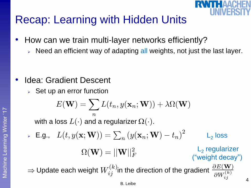
Recap: Learning with Hidden Units

• How can we train multi-layer networks efficiently?

Need an efficient way of adapting all weights, not just the last layer.

• Idea: Gradient Descent

Set up an error function

with a loss L(¢) and a regularizer (¢).

E.g.,

Update each weight in the direction of the gradient

4B. Leibe

L2 loss

L2 regularizer

(“weight decay”)

Perc

ep

tual

an

d S

en

so

ry A

ug

me

nte

d C

om

pu

tin

gM

achin

e L

earn

ing W

inte

r ‘1

7

Gradient Descent

• Two main steps

1. Computing the gradients for each weight

2. Adjusting the weights in the direction of

the gradient

5B. Leibe

last lecture

today

Perc

ep

tual

an

d S

en

so

ry A

ug

me

nte

d C

om

pu

tin

gM

achin

e L

earn

ing W

inte

r ‘1

7

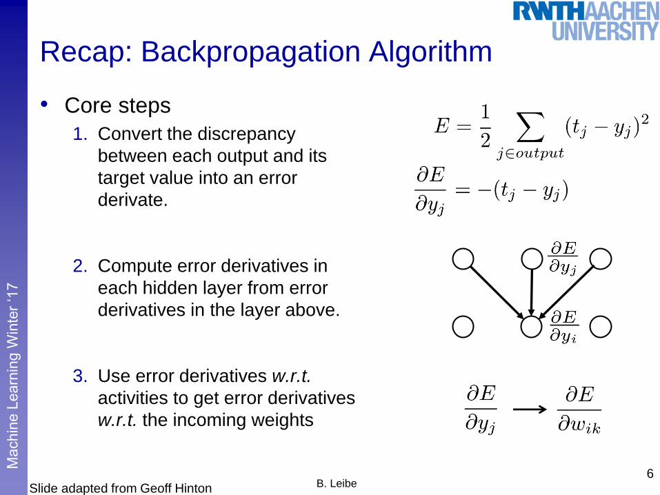
Recap: Backpropagation Algorithm

• Core steps

1. Convert the discrepancy

between each output and its

target value into an error

derivate.

2. Compute error derivatives in

each hidden layer from error

derivatives in the layer above.

3. Use error derivatives w.r.t.

activities to get error derivatives

w.r.t. the incoming weights

6B. LeibeSlide adapted from Geoff Hinton

Perc

ep

tual

an

d S

en

so

ry A

ug

me

nte

d C

om

pu

tin

gM

achin

e L

earn

ing W

inte

r ‘1

7

• Efficient propagation scheme

yi is already known from forward pass! (Dynamic Programming)

Propagate back the gradient from layer j and multiply with yi.

Recap: Backpropagation Algorithm


Perc

ep

tual

an

d S

en

so

ry A

ug

me

nte

d C

om

pu

tin

gM

achin

e L

earn

ing W

inte

r ‘1

7

Recap: MLP Backpropagation Algorithm

• Forward Pass

for k = 1, ..., l do

endfor

• Notes

For efficiency, an entire batch of data X is processed at once.

¯ denotes the element-wise product

8B. Leibe

• Backward Pass

for k = l, l-1, ...,1 do

endfor

Perc

ep

tual

an

d S

en

so

ry A

ug

me

nte

d C

om

pu

tin

gM

achin

e L

earn

ing W

inte

r ‘1

7





Practical issues



Momentum

RMS Prop

Other Optimizers


Data Augmentation


Perc

ep

tual

an

d S

en

so

ry A

ug

me

nte

d C

om

pu

tin

gM

achin

e L

earn

ing W

inte

r ‘1

7

Computational Graphs

• We can think of mathematical expressions as graphs

E.g., consider the expression

We can decompose this into

the operations

and visualize this as a computational graph.

• Evaluating partial derivatives in such a graph

General rule: sum over all possible paths from Y to X

and multiply the derivatives on each edge of the path together.

10B. LeibeSlide inspired by Christopher Olah Image source: Christopher Olah, colah.github.io

Perc

ep

tual

an

d S

en

so

ry A

ug

me

nte

d C

om

pu

tin

gM

achin

e L

earn

ing W

inte

r ‘1

7

Factoring Paths

• Problem: Combinatorial explosion

Example:

There are 3 paths from X to Y and 3 more from Y to Z.

If we want to compute , we need to sum over 3£3 paths:

Instead of naively summing over paths, it’s better to factor them


Perc

ep

tual

an

d S

en

so

ry A

ug

me

nte

d C

om

pu

tin

gM

achin

e L

earn

ing W

inte

r ‘1

7

Efficient Factored Algorithms

• Efficient algorithms for computing the sum

Instead of summing over all of the paths explicitly, compute

the sum more efficiently by merging paths back together at

every node. 12

B. Leibe

Apply operator

to every node.

Apply operator

to every node.

Slide inspired by Christopher Olah Image source: Christopher Olah, colah.github.io

Perc

ep

tual

an

d S

en

so

ry A

ug

me

nte

d C

om

pu

tin

gM

achin

e L

earn

ing W

inte

r ‘1

7

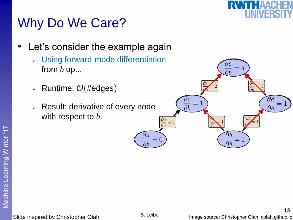
Why Do We Care?

• Let’s consider the example again

Using forward-mode differentiation

from b up...

Runtime: O(#edges)

Result: derivative of every node

with respect to b.


Perc

ep

tual

an

d S

en

so

ry A

ug

me

nte

d C

om

pu

tin

gM

achin

e L

earn

ing W

inte

r ‘1

7

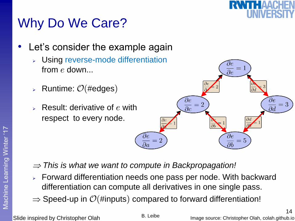
Why Do We Care?


• Let’s consider the example again

Using reverse-mode differentiation

from e down...

Runtime: O(#edges)

Result: derivative of e with

respect to every node.

This is what we want to compute in Backpropagation!

Forward differentiation needs one pass per node. With backward

differentiation can compute all derivatives in one single pass.

Speed-up in O(#inputs) compared to forward differentiation!

Perc

ep

tual

an

d S

en

so

ry A

ug

me

nte

d C

om

pu

tin

gM

achin

e L

earn

ing W

inte

r ‘1

7





Practical issues



Momentum

RMS Prop

Other Optimizers


Data Augmentation


Perc

ep

tual

an

d S

en

so

ry A

ug

me

nte

d C

om

pu

tin

gM

achin

e L

earn

ing W

inte

r ‘1

7

Obtaining the Gradients

• Approach 4: Automatic Differentiation

Convert the network into a computational graph.

Each new layer/module just needs to specify how it affects the

forward and backward passes.

Apply reverse-mode differentiation.

Very general algorithm, used in today’s Deep Learning packages16

B. Leibe

Perc

ep

tual

an

d S

en

so

ry A

ug

me

nte

d C

om

pu

tin

gM

achin

e L

earn

ing W

inte

r ‘1

7

Modular Implementation

• Solution in many current Deep Learning libraries

Provide a limited form of automatic differentiation

Restricted to “programs” composed of “modules” with a

predefined set of operations.

• Each module is defined by two main functions

1. Computing the outputs y of the module given its inputs x

where x, y, and intermediate results are stored in the module.

2. Computing the gradient E/x of a scalar cost w.r.t. the

inputs x given the gradient E/y w.r.t. the outputs y

17B. Leibe

Perc

ep

tual

an

d S

en

so

ry A

ug

me

nte

d C

om

pu

tin

gM

achin

e L

earn

ing W

inte

r ‘1

7





Practical issues



Momentum

RMS Prop

Other Optimizers


Data Augmentation


Perc

ep

tual

an

d S

en

so

ry A

ug

me

nte

d C

om

pu

tin

gM

achin

e L

earn

ing W

inte

r ‘1

7

Implementing Softmax Correctly

• Softmax output

De-facto standard for multi-class outputs

• Practical issue

Exponentials get very big and can have vastly different magnitudes.

Trick 1: Do not compute first softmax, then log,

but instead directly evaluate log-exp in the denominator.

Trick 2: Softmax has the property that for a fixed vector b

Subtract the largest weight vector wj from the others.

19B. Leibe

E(w) = ¡NX

n=1

KX

k=1

(I (tn = k) ln

exp(w>k x)PK

j=1 exp(w>j x)

)

Perc

ep

tual

an

d S

en

so

ry A

ug

me

nte

d C

om

pu

tin

gM

achin

e L

earn

ing W

inte

r ‘1

7





Practical issues



Momentum

RMS Prop

Other Optimizers


Data Augmentation


Perc

ep

tual

an

d S

en

so

ry A

ug

me

nte

d C

om

pu

tin

gM

achin

e L

earn

ing W

inte

r ‘1

7

Gradient Descent

• Two main steps

1. Computing the gradients for each weight

2. Adjusting the weights in the direction of

the gradient

• Recall: Basic update equation

• Main questions

On what data do we want to apply this?

How should we choose the step size ´ (the learning rate)?

In which direction should we update the weights?21

B. Leibe

last lecture

today

w(¿+1)

kj = w(¿)

kj ¡ ´@E(w)

@wkj

¯̄¯̄w(¿)

Perc

ep

tual

an

d S

en

so

ry A

ug

me

nte

d C

om

pu

tin

gM

achin

e L

earn

ing W

inte

r ‘1

7

Stochastic vs. Batch Learning

• Batch learning

Process the full dataset at

once to compute the

gradient.

• Stochastic learning

Choose a single example

from the training set.

Compute the gradient only

based on this example

This estimate will generally

be noisy, which has some

advantages.22

B. Leibe

w(¿+1)

kj = w(¿)

kj ¡ ´@E(w)

@wkj

¯̄¯̄w(¿)

w(¿+1)

kj = w(¿)

kj ¡ ´@En(w)

@wkj

¯̄¯̄w(¿)

Perc

ep

tual

an

d S

en

so

ry A

ug

me

nte

d C

om

pu

tin

gM

achin

e L

earn

ing W

inte

r ‘1

7

Stochastic vs. Batch Learning

• Batch learning advantages

Conditions of convergence are well understood.

Many acceleration techniques (e.g., conjugate gradients) only

operate in batch learning.

Theoretical analysis of the weight dynamics and convergence rates

are simpler.

• Stochastic learning advantages

Usually much faster than batch learning.

Often results in better solutions.

Can be used for tracking changes.

• Middle ground: Minibatches

23B. Leibe

Perc

ep

tual

an

d S

en

so

ry A

ug

me

nte

d C

om

pu

tin

gM

achin

e L

earn

ing W

inte

r ‘1

7

Minibatches

• Idea

Process only a small batch of training examples together

Start with a small batch size & increase it as training proceeds.

• Advantages

Gradients will more stable than for stochastic gradient descent,

but still faster to compute than with batch learning.

Take advantage of redundancies in the training set.

Matrix operations are more efficient than vector operations.

• Caveat

Error function should be normalized by the minibatch size,

s.t. we can keep the same learning rate between minibatches

24B. Leibe

Perc

ep

tual

an

d S

en

so

ry A

ug

me

nte

d C

om

pu

tin

gM

achin

e L

earn

ing W

inte

r ‘1

7





Practical issues



Momentum

RMS Prop

Other Optimizers


Data Augmentation


Perc

ep

tual

an

d S

en

so

ry A

ug

me

nte

d C

om

pu

tin

gM

achin

e L

earn

ing W

inte

r ‘1

7

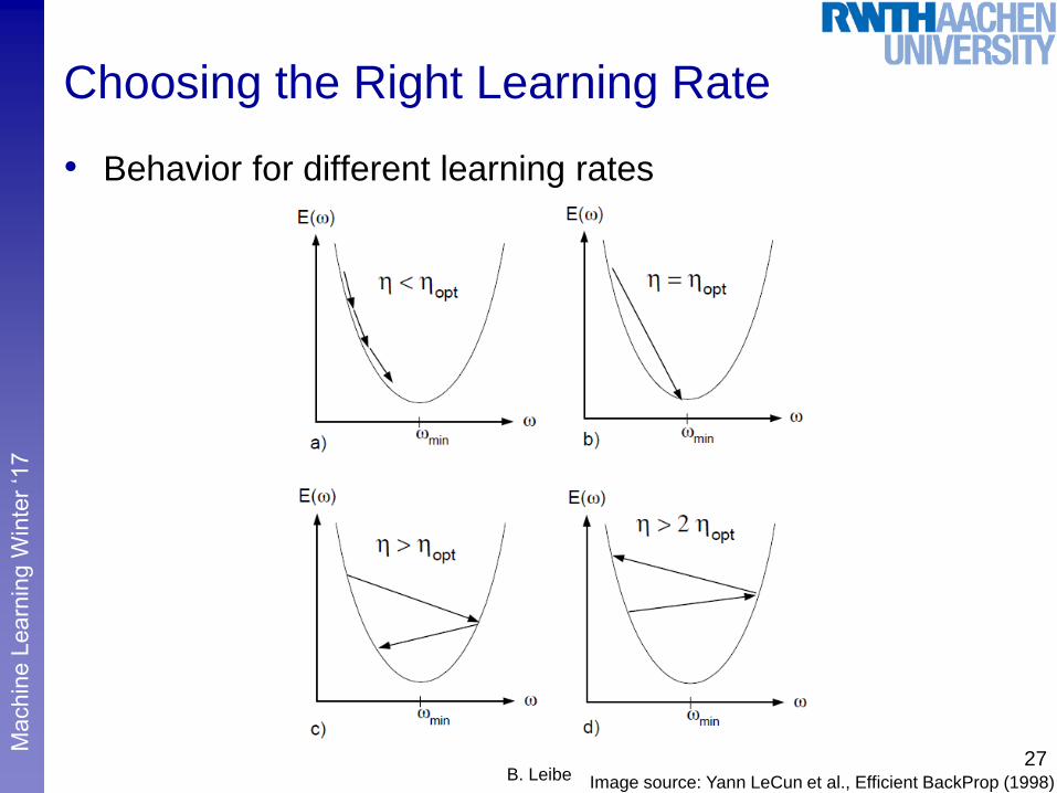
Choosing the Right Learning Rate

• Analyzing the convergence of Gradient Descent

Consider a simple 1D example first

What is the optimal learning rate ´opt?

If E is quadratic, the optimal learning rate is given by the inverse of

the Hessian

What happens if we exceed this learning rate?

26B. Leibe Image source: Yann LeCun et al., Efficient BackProp (1998)

Perc

ep

tual

an

d S

en

so

ry A

ug

me

nte

d C

om

pu

tin

gM

achin

e L

earn

ing W

inte

r ‘1

7

Choosing the Right Learning Rate

• Behavior for different learning rates


Perc

ep

tual

an

d S

en

so

ry A

ug

me

nte

d C

om

pu

tin

gM

achin

e L

earn

ing W

inte

r ‘1

7

Learning Rate vs. Training Error

28B. Leibe Image source: Goodfellow & Bengio book

Do not go beyond

this point!

Perc

ep

tual

an

d S

en

so

ry A

ug

me

nte

d C

om

pu

tin

gM

achin

e L

earn

ing W

inte

r ‘1

7





Practical issues



Momentum

RMS Prop

Other Optimizers


Data Augmentation


Perc

ep

tual

an

d S

en

so

ry A

ug

me

nte

d C

om

pu

tin

gM

achin

e L

earn

ing W

inte

r ‘1

7

Batch vs. Stochastic Learning

• Batch Learning

Simplest case: steepest decent

on the error surface.

Updates perpendicular to contour

lines

• Stochastic Learning

Simplest case: zig-zag around the

direction of steepest descent.

Updates perpendicular to constraints

from training examples.

30B. Leibe Image source: Geoff HintonSlide adapted from Geoff Hinton

Perc

ep

tual

an

d S

en

so

ry A

ug

me

nte

d C

om

pu

tin

gM

achin

e L

earn

ing W

inte

r ‘1

7

Why Learning Can Be Slow

• If the inputs are correlated

The ellipse will be very elongated.

The direction of steepest descent is

almost perpendicular to the direction

towards the minimum!

This is just the opposite of what we want!

31B. Leibe Image source: Geoff HintonSlide adapted from Geoff Hinton

Perc

ep

tual

an

d S

en

so

ry A

ug

me

nte

d C

om

pu

tin

gM

achin

e L

earn

ing W

inte

r ‘1

7

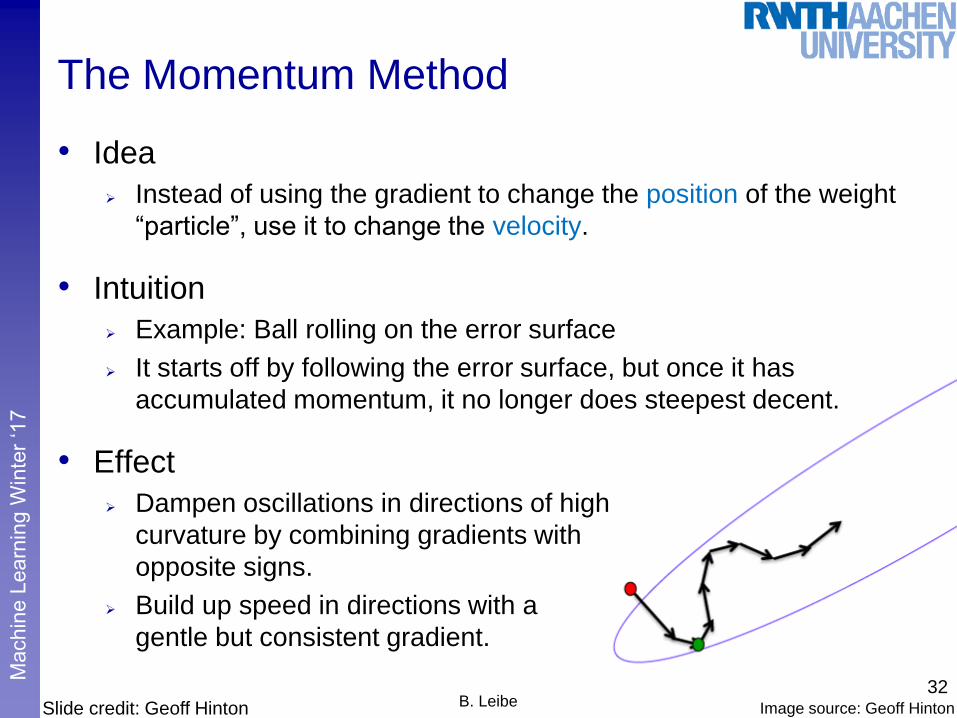
The Momentum Method

• Idea

Instead of using the gradient to change the position of the weight

“particle”, use it to change the velocity.

• Intuition

Example: Ball rolling on the error surface

It starts off by following the error surface, but once it has

accumulated momentum, it no longer does steepest decent.

• Effect

Dampen oscillations in directions of high

curvature by combining gradients with

opposite signs.

Build up speed in directions with a

gentle but consistent gradient.

32B. Leibe Image source: Geoff HintonSlide credit: Geoff Hinton

Perc

ep

tual

an

d S

en

so

ry A

ug

me

nte

d C

om

pu

tin

gM

achin

e L

earn

ing W

inte

r ‘1

7

The Momentum Method: Implementation

• Change in the update equations

Effect of the gradient: increment the previous velocity, subject to a

decay by ® < 1.

Set the weight change to the current velocity

33B. LeibeSlide credit: Geoff Hinton

Perc

ep

tual

an

d S

en

so

ry A

ug

me

nte

d C

om

pu

tin

gM

achin

e L

earn

ing W

inte

r ‘1

7

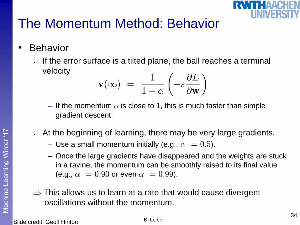
The Momentum Method: Behavior

• Behavior

If the error surface is a tilted plane, the ball reaches a terminal

velocity

– If the momentum ® is close to 1, this is much faster than simple

gradient descent.

At the beginning of learning, there may be very large gradients.

– Use a small momentum initially (e.g., ® = 0.5).

– Once the large gradients have disappeared and the weights are stuck

in a ravine, the momentum can be smoothly raised to its final value

(e.g., ® = 0.90 or even ® = 0.99).

This allows us to learn at a rate that would cause divergent

oscillations without the momentum.

34B. LeibeSlide credit: Geoff Hinton

Perc

ep

tual

an

d S

en

so

ry A

ug

me

nte

d C

om

pu

tin

gM

achin

e L

earn

ing W

inte

r ‘1

7

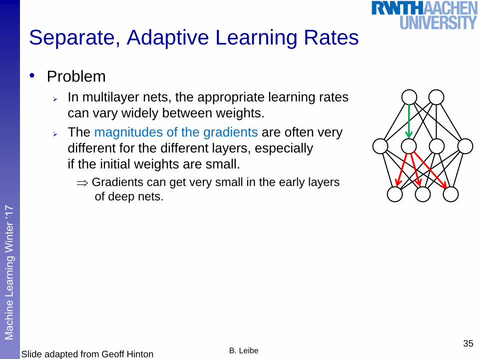
Separate, Adaptive Learning Rates

• Problem

In multilayer nets, the appropriate learning rates

can vary widely between weights.

The magnitudes of the gradients are often very

different for the different layers, especially

if the initial weights are small.

Gradients can get very small in the early layers

of deep nets.


Perc

ep

tual

an

d S

en

so

ry A

ug

me

nte

d C

om

pu

tin

gM

achin

e L

earn

ing W

inte

r ‘1

7

Separate, Adaptive Learning Rates

• Problem

In multilayer nets, the appropriate learning rates

can vary widely between weights.

The magnitudes of the gradients are often very

different for the different layers, especially

if the initial weights are small.

Gradients can get very small in the early layers

of deep nets.

The fan-in of a unit determines the size of the

“overshoot” effect when changing multiple weights

simultaneously to correct the same error.

– The fan-in often varies widely between layers

• Solution

Use a global learning rate, multiplied by a local gain per weight

(determined empirically)36

B. LeibeSlide adapted from Geoff Hinton

Perc

ep

tual

an

d S

en

so

ry A

ug

me

nte

d C

om

pu

tin

gM

achin

e L

earn

ing W

inte

r ‘1

7

Better Adaptation: RMSProp

• Motivation

The magnitude of the gradient can be very different for different

weights and can change during learning.

This makes it hard to choose a single global learning rate.

For batch learning, we can deal with this by only using the sign of the

gradient, but we need to generalize this for minibatches.

• Idea of RMSProp

Divide the gradient by a running average of its recent magnitude

Divide the gradient by sqrt(MeanSq(wij,t)).


Perc

ep

tual

an

d S

en

so

ry A

ug

me

nte

d C

om

pu

tin

gM

achin

e L

earn

ing W

inte

r ‘1

7

Other Optimizers

• AdaGrad [Duchi ’10]

• AdaDelta [Zeiler ’12]

• Adam [Ba & Kingma ’14]

• Notes

All of those methods have the goal to make the optimization less

sensitive to parameter settings.

Adam is currently becoming the quasi-standard

38B. Leibe

Perc

ep

tual

an

d S

en

so

ry A

ug

me

nte

d C

om

pu

tin

gM

achin

e L

earn

ing W

inte

r ‘1

7

Behavior in a Long Valley

39B. Leibe Image source: Aelc Radford, http://imgur.com/a/Hqolp

Perc

ep

tual

an

d S

en

so

ry A

ug

me

nte

d C

om

pu

tin

gM

achin

e L

earn

ing W

inte

r ‘1

7

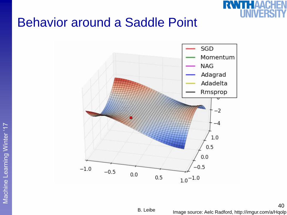
Behavior around a Saddle Point

40B. Leibe Image source: Aelc Radford, http://imgur.com/a/Hqolp

Perc

ep

tual

an

d S

en

so

ry A

ug

me

nte

d C

om

pu

tin

gM

achin

e L

earn

ing W

inte

r ‘1

7

Visualization of Convergence Behavior

41B. Leibe Image source: Aelc Radford, http://imgur.com/SmDARzn

Perc

ep

tual

an

d S

en

so

ry A

ug

me

nte

d C

om

pu

tin

gM

achin

e L

earn

ing W

inte

r ‘1

7

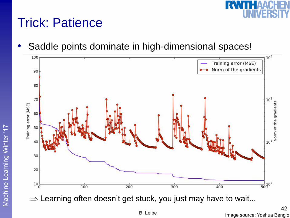
Trick: Patience

• Saddle points dominate in high-dimensional spaces!

Learning often doesn’t get stuck, you just may have to wait...42

B. Leibe Image source: Yoshua Bengio

Perc

ep

tual

an

d S

en

so

ry A

ug

me

nte

d C

om

pu

tin

gM

achin

e L

earn

ing W

inte

r ‘1

7

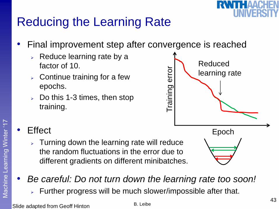
Reducing the Learning Rate

• Final improvement step after convergence is reached

Reduce learning rate by a

factor of 10.

Continue training for a few

epochs.

Do this 1-3 times, then stop

training.

• Effect

Turning down the learning rate will reduce

the random fluctuations in the error due to

different gradients on different minibatches.

• Be careful: Do not turn down the learning rate too soon!

Further progress will be much slower/impossible after that.43

B. Leibe

Reduced

learning rate

Tra

inin

g e

rro

r

Epoch

Slide adapted from Geoff Hinton

Perc

ep

tual

an

d S

en

so

ry A

ug

me

nte

d C

om

pu

tin

gM

achin

e L

earn

ing W

inte

r ‘1

7

Summary

• Deep multi-layer networks are very powerful.

• But training them is hard!

Complex, non-convex learning problem

Local optimization with stochastic gradient descent

• Main issue: getting good gradient updates for the lower

layers of the network

Many seemingly small details matter!

Weight initialization, normalization, data augmentation, choice of

nonlinearities, choice of learning rate, choice of optimizer,…

In the following, we will take a look at the most important factors

(to be continued in the next lecture…)

44B. Leibe

Perc

ep

tual

an

d S

en

so

ry A

ug

me

nte

d C

om

pu

tin

gM

achin

e L

earn

ing W

inte

r ‘1

7





Practical issues



Momentum

RMS Prop

Other Optimizers


Data Augmentation


Perc

ep

tual

an

d S

en

so

ry A

ug

me

nte

d C

om

pu

tin

gM

achin

e L

earn

ing W

inte

r ‘1

7

Shuffling the Examples

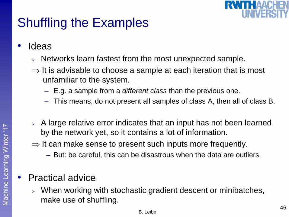
• Ideas

Networks learn fastest from the most unexpected sample.

It is advisable to choose a sample at each iteration that is most

unfamiliar to the system.

– E.g. a sample from a different class than the previous one.

– This means, do not present all samples of class A, then all of class B.

A large relative error indicates that an input has not been learned

by the network yet, so it contains a lot of information.

It can make sense to present such inputs more frequently.

– But: be careful, this can be disastrous when the data are outliers.

• Practical advice

When working with stochastic gradient descent or minibatches,

make use of shuffling.46

B. Leibe

Perc

ep

tual

an

d S

en

so

ry A

ug

me

nte

d C

om

pu

tin

gM

achin

e L

earn

ing W

inte

r ‘1

7

Data Augmentation

• Idea

Augment original data with synthetic variations

to reduce overfitting

• Example augmentations for images

Cropping

Zooming

Flipping

Color PCA

47B. Leibe Image source: Lucas Beyer

Perc

ep

tual

an

d S

en

so

ry A

ug

me

nte

d C

om

pu

tin

gM

achin

e L

earn

ing W

inte

r ‘1

7

Data Augmentation

• Effect

Much larger training set

Robustness against expected

variations

• During testing

When cropping was used

during training, need to

again apply crops to get

same image size.

Beneficial to also apply

flipping during test.

Applying several ColorPCA

variations can bring another

~1% improvement, but at a

significantly increased runtime.48

B. Leibe

Augmented training data

(from one original image)

Image source: Lucas Beyer

Perc

ep

tual

an

d S

en

so

ry A

ug

me

nte

d C

om

pu

tin

gM

achin

e L

earn

ing W

inte

r ‘1

7

Practical Advice

49B. Leibe

Perc

ep

tual

an

d S

en

so

ry A

ug

me

nte

d C

om

pu

tin

gM

achin

e L

earn

ing W

inte

r ‘1

7

Normalization

• Motivation

Consider the Gradient Descent update steps

From backpropagation, we know that

When all of the components of the input vector yi are positive, all of

the updates of weights that feed into a node will be of the same sign.

Weights can only all increase or decrease together.

Slow convergence

50B. Leibe

w(¿+1)

kj = w(¿)

kj ¡ ´@E(w)

@wkj

¯̄¯̄w(¿)

Perc

ep

tual

an

d S

en

so

ry A

ug

me

nte

d C

om

pu

tin

gM

achin

e L

earn

ing W

inte

r ‘1

7

Normalizing the Inputs

• Convergence is fastest if

The mean of each input variable

over the training set is zero.

The inputs are scaled such that

all have the same covariance.

Input variables are uncorrelated

if possible.

• Advisable normalization steps (for MLPs only, not for CNNs)

Normalize all inputs that an input unit sees to zero-mean,

unit covariance.

If possible, try to decorrelate them using PCA (also known as

Karhunen-Loeve expansion).


Perc

ep

tual

an

d S

en

so

ry A

ug

me

nte

d C

om

pu

tin

gM

achin

e L

earn

ing W

inte

r ‘1

7

References and Further Reading

• More information on many practical tricks can be found in

Chapter 1 of the book

52B. Leibe

G. Montavon, G. B. Orr, K-R Mueller (Eds.)

Neural Networks: Tricks of the Trade

Springer, 1998, 2012

Yann LeCun, Leon Bottou, Genevieve B. Orr, Klaus-Robert Mueller

Efficient BackProp, Ch.1 of the above book., 1998.

http://n.lecun.com/exdb/publis/pdf/lecun-98b.pdf

Machine Learning Lecture 13 - Computer Vision€¦ · · 2017-12-04Machine Learning –Lecture 13 Neural Networks II 04.12.2017 Bastian Leibe RWTH Aachen [email protected].

Documents