Yasemin Altun · Kamalika Das Taneli Mielikäinen · Donato Malerba Jerzy Stefanowski · Jesse Read Marinka Žitnik · Michelangelo Ceci Sašo Džeroski (Eds.) 123 LNAI 10536 European Conference, ECML PKDD 2017 Skopje, Macedonia, September 18–22, 2017 Proceedings, Part III Machine Learning and Knowledge Discovery in Databases

Welcome message from author
This document is posted to help you gain knowledge. Please leave a comment to let me know what you think about it! Share it to your friends and learn new things together.
Transcript

Yasemin Altun · Kamalika DasTaneli Mielikäinen · Donato MalerbaJerzy Stefanowski · Jesse ReadMarinka Žitnik · Michelangelo CeciSašo Džeroski (Eds.)
123
LNAI
105
36
European Conference, ECML PKDD 2017Skopje, Macedonia, September 18–22, 2017Proceedings, Part III
Machine Learning andKnowledge Discoveryin Databases

Lecture Notes in Artificial Intelligence 10536
Subseries of Lecture Notes in Computer Science
LNAI Series Editors
Randy GoebelUniversity of Alberta, Edmonton, Canada
Yuzuru TanakaHokkaido University, Sapporo, Japan
Wolfgang WahlsterDFKI and Saarland University, Saarbrücken, Germany
LNAI Founding Series Editor
Joerg SiekmannDFKI and Saarland University, Saarbrücken, Germany

More information about this series at http://www.springer.com/series/1244

Yasemin Altun • Kamalika DasTaneli Mielikäinen • Donato MalerbaJerzy Stefanowski • Jesse ReadMarinka Žitnik • Michelangelo CeciSašo Džeroski (Eds.)
Machine Learning andKnowledge Discoveryin DatabasesEuropean Conference, ECML PKDD 2017Skopje, Macedonia, September 18–22, 2017Proceedings, Part III
123

EditorsYasemin AltunGoogle ResearchGoogle Inc.ZurichSwitzerland
Kamalika DasNASA Ames Research CenterMountain ViewUSA
Taneli MielikäinenOathSunnyvaleUSA
Donato MalerbaDepartment of Computer ScienceUniversity of Bari Aldo MoroBariItaly
Jerzy StefanowskiInstitute of Computing SciencePoznan University of TechnologyPoznanPoland
Jesse ReadLaboratoire d’ Informatique (LIX)École PolytechniquePalaiseauFrance
Marinka ŽitnikDepartment of Computer ScienceStanford UniversityStanfordUSA
Michelangelo CeciUniversità degli Studi di Bari Aldo MoroBariItaly
Sašo DžeroskiJožef Stefan InstituteLjubljanaSlovenia
ISSN 0302-9743 ISSN 1611-3349 (electronic)Lecture Notes in Artificial IntelligenceISBN 978-3-319-71272-7 ISBN 978-3-319-71273-4 (eBook)https://doi.org/10.1007/978-3-319-71273-4
Library of Congress Control Number: 2017961799
LNCS Sublibrary: SL7 – Artificial Intelligence
© Springer International Publishing AG 2017This work is subject to copyright. All rights are reserved by the Publisher, whether the whole or part of thematerial is concerned, specifically the rights of translation, reprinting, reuse of illustrations, recitation,broadcasting, reproduction on microfilms or in any other physical way, and transmission or informationstorage and retrieval, electronic adaptation, computer software, or by similar or dissimilar methodology nowknown or hereafter developed.The use of general descriptive names, registered names, trademarks, service marks, etc. in this publicationdoes not imply, even in the absence of a specific statement, that such names are exempt from the relevantprotective laws and regulations and therefore free for general use.The publisher, the authors and the editors are safe to assume that the advice and information in this book arebelieved to be true and accurate at the date of publication. Neither the publisher nor the authors or the editorsgive a warranty, express or implied, with respect to the material contained herein or for any errors oromissions that may have been made. The publisher remains neutral with regard to jurisdictional claims inpublished maps and institutional affiliations.
Printed on acid-free paper
This Springer imprint is published by Springer NatureThe registered company is Springer International Publishing AGThe registered company address is: Gewerbestrasse 11, 6330 Cham, Switzerland

Preface
This year was the 10th edition of ECML PKDD as a single conference. While ECMLand PKDD have been organized jointly since 2001, they only officially merged in2008. Following the growth of the field and the community, the conference hasdiversified and expanded over the past decade in terms of content, form, and atten-dance. This year, ECML PKDD attracted over 600 participants.
We were proud to present a rich scientific program, including high-profile keynotesand many technical presentations in different tracks (research, journal, applied datascience, nectar, and demo), fora (EU projects, PhD), workshops, tutorials, and dis-covery challenges. We hope that this provided ample opportunities for excitingexchanges of ideas and pleasurable networking.
Many people put in countless hours of work to make this event happen: To them weexpress our heartfelt thanks. This includes the organization team, i.e., the programchairs of the different tracks and fora, workshops and tutorials, and discovery chal-lenges, as well as the awards committee, production and public relations chairs, localorganizers, sponsorship chairs, and proceedings chairs. In addition, we would like tothank the program committees of the different conference tracks, the organizers of theworkshops and their respective committees, the Cankarjev Dom congress agency, andthe student volunteers. Furthermore, many thanks to our sponsors for their generousfinancial support. We would also like to thank Springer for their continuous support,Microsoft for allowing us to use their CMT software for conference management, theEuropean project MAESTRA (ICT-2013-612944), as well as the ECML PKDDSteering Committee (for their suggestions and advice). We would like to thank theorganizing institutions: the Jožef Stefan Institute (Slovenia), the Ss. Cyril andMethodius University in Skopje (Macedonia), and the University of Bari Aldo Moro(Italy).
Finally, thanks to all authors who submitted their work for presentation atECML PKDD 2017. Last, but certainly not least, we would like to thank the conferenceparticipants who helped us make it a memorable event.
September 2017 Sašo DžeroskiMichelangelo Ceci

Foreword to the ECML PKDD 2017Applied Data Science Track
We are pleased to present the proceedings of the Applied Data Science (ADS) Track ofECML PKDD 2017. This track aims to bring together participants from academia,industry, governments, and NGOs (non-governmental organizations) in a venue thathighlights practical and real-world studies of machine learning, knowledge discovery,and data mining. Novel and practical ideas, open problems in applied data science,description of application-specific challenges, and unique solutions adopted in bridgingthe gap between research and practice are some of the relevant topics for which papershave been submitted and accepted in this track. This year’s Applied Data Science Trackincluded 27 accepted paper presentations distributed across six sessions. Given a totalof 93 submissions, this year’s track was highly selective: Only 27 papers could beaccepted for publication and for presentation at the conference, corresponding to anacceptance rate of 29%. Each of the 93 submissions was thoroughly reviewed, andaccepted papers were chosen both for their originality and for the application theypromoted. The accepted papers focus on topics ranging from machine-learning meth-ods and data science processes to dedicated applications. Topics covered include deeplearning, time series mining, text mining, for a variety of applications such ase-commerce, fraud detection, social good, ecology, experiment design, and socialnetwork analysis. We thank all the authors who submitted the 93 papers for their workand effort to bring machine learning to solve many interesting problems. We also thankall the Program Committee members of the ADS track for their substantial efforts toguarantee the quality of these proceedings. We hope that this program was enjoyable toboth academics and practitioners alike, and fostered the beginning of new industry–academia collaborations.
September 2017 Yasemin AltunKamalika Das
Taneli Mielikäinen

Foreword to the ECML PKDD 2017 Nectar Track
We are pleased to present the proceedings of the Nectar Track of the ECML PKDD2017 conference held in Skopje. This track, which started in 2012, provides a forum forthe discussion of recent high-quality research results at the frontier of machine learningand data mining with other disciplines, which have been already published in relatedconferences and journals. For researchers from the other disciplines, the Nectar Trackoffers a place to present their work to the ECML PKDD community and to raise thecommunity’s awareness of data analysis results and open problems in their field.Particularly welcome were papers illustrating the pervasiveness of data-driven explo-ration and modelling in science, technology, and society, as well as innovativeapplications, and also theoretical results. Authors were invited to submit four-pagesummaries of their previously published work.
We received 25 submissions and each of them was thoroughly reviewed by twoProgram Committee (PC) members. Finally, ten papers were selected for publication inthe proceedings and presentation during the conference. The accepted papers cover awide range of machine learning and data mining methods, as well as quite diversedomains of applications. The topics cover, among others, automatic music generation,music chord prediction, phenotype inference from biomedical texts and genomicdatabases, new data-driven approaches for finding a parking space in cities,process-based modelling to construct dynamical systems, advances in kernel-basedgraph classification, user interactions and influence in social networks, efficientexploitation of tree ensembles in Web search and document ranking, data cleaning withAI planning solvers, and applications of predictive clustering trees to image analysis.
We take this opportunity to thank all authors for submitting their papers to theNectar Track. We also wish to express our gratitude to all PC members who helped usin the reviewing process, providing insightful feedback that helped the authors ofaccepted papers to prepare good presentations during the conference. Finally, we wouldlike to thank the ECML PKDD general chairs and the other members of the OrganizingCommittee for their excellent co-operation and support for all our efforts. We hope thatthe readers will enjoy these short papers and that the papers, conference presentations,and discussions will inspire further interesting research at the boundaries of machinelearning and data mining with many other interesting fields.
September 2017 Donato MalerbaJerzy Stefanowski

Foreword to the ECML PKDD 2017 Demo Track
We present, with great pleasure, the Demo Track of ECML PKDD 2017. Since itsinception, this Demo Track is among the major forums in the field for presentingstate-of-the-art data mining and machine learning systems and research prototypes, andfor disseminating new methods and techniques in a variety of application domains.Each selected demo was presented at the conference and allocated a four-page paper inthe proceedings.
The evaluation criteria encompassed innovation and technical advances, meetingnovel challenges, and the potential impact and interest for researchers and practitionersin the machine learning and data-mining community. Each submission was firstreviewed by at least two expert referees, with a majority receiving three reviews.Consensus on each paper was reached through discussion between the demo chairs. Intotal, 52 reviews were made, and from 17 original submissions 10 were accepted forpublication in the conference proceedings and presentation at the demo sessions duringthe conference in Skopje. The accepted demonstration papers cover a wide range ofmachine learning and data mining techniques, as well as a very diverse set ofreal-world application domains. We believe the review system was successful inensuring that the accepted work is of high quality and suited for publication in thetrack.
We thank all authors for submitting their work, without which this track would notbe possible. We are deeply grateful to our Program Committee for volunteering theirtime and expertise. Their contribution is at the core of the scientific quality of the DemoTrack. The expert Program Committee included a mix of experienced individuals fromprevious years as well as experts newly recruited to ensure broad technical expertiseand to promote inclusivity of various data mining and machine learning research areas.Finally, we wish to thank the general chairs and the program chairs for entrusting uswith this track and providing us with their expert advice. We hope that the readers willenjoy this set of short papers and that the demonstrated systems, prototypes, andlibraries of this track will inspire interaction and discussion that will be valuable to boththe authors and the community at large.
September 2017 Jesse ReadMarinka Zitnik

Organization
ECML PKDD 2017 Organization
Conference Chairs
Michelangelo Ceci University of Bari Aldo Moro, ItalySašo Džeroski Jožef Stefan Institute, Slovenia
Program Chairs
Michelangelo Ceci University of Bari Aldo Moro, ItalyJaakko Hollmén Aalto University, FinlandLjupčo Todorovski University of Ljubljana, SloveniaCeline Vens KU Leuven Kulak, Belgium
Journal Track Chairs
Kurt Driessens Maastricht University, The NetherlandsDragi Kocev Jožef Stefan Institute, SloveniaMarko Robnik-Šikonja University of Ljubljana, SloveniaMyra Spiliopoulu Magdeburg University, Germany
Applied Data Science Track Chairs
Yasemin Altun Google Research, SwitzerlandKamalika Das NASA Ames Research Center, USATaneli Mielikäinen Yahoo! USA
Local Organization Chairs
Ivica Dimitrovski Ss. Cyril and Methodius University, MacedoniaTina Anžič Jožef Stefan Institute, SloveniaMili Bauer Jožef Stefan Institute, SloveniaGjorgji Madjarov Ss. Cyril and Methodius University, Macedonia
Workshops and Tutorials Chairs
Nathalie Japkowicz American University, USAPanče Panov Jožef Stefan Institute, Slovenia

Awards Committee
Peter Flach University of Bristol, UKRosa Meo University of Turin, ItalyIndrė Žliobaitė University of Helsinki, Finland
Nectar Track Chairs
Donato Malerba University of Bari Aldo Moro, ItalyJerzy Stefanowski Poznan University of Technology, Poland
Demo Track Chairs
Jesse Read École Polytechnique, FranceMarinka Žitnik Stanford University, USA
PhD Forum Chairs
Tomislav Šmuc Rudjer Bošković Institute, CroatiaBernard Ženko Jožef Stefan Institute, Slovenia
EU Projects Forum Chairs
Petra Kralj Novak Jožef Stefan Institute, SloveniaNada Lavrač Jožef Stefan Institute, Slovenia
Proceedings Chairs
Jurica Levatić Jožef Stefan Institute, SloveniaGianvito Pio University of Bari Aldo Moro, Italy
Discovery Challenge Chair
Dino Ienco IRSTEA - UMR TETIS, France
Sponsorship Chairs
Albert Bifet Télécom ParisTech, FrancePanče Panov Jožef Stefan Institute, Slovenia
Production and Public Relations Chairs
Dragi Kocev Jožef Stefan Institute, SloveniaNikola Simidjievski Jožef Stefan Institute, Slovenia
XIV Organization

ECML PKDD Steering Committee
Michele Sebag Université Paris Sud, FranceFrancesco Bonchi ISI Foundation, ItalyAlbert Bifet Télécom ParisTech, FranceHendrik Blockeel KU Leuven, Belgium and Leiden University,
The NetherlandsKatharina Morik University of Dortmund, GermanyArno Siebes Utrecht University, The NetherlandsSiegfried Nijssen LIACS, Leiden University, The NetherlandsChedy Raïssi Inria Nancy Grand-Est, FranceRosa Meo Università di Torino, ItalyToon Calders Eindhoven University of Technology, The NetherlandsJoão Gama FCUP, University of Porto/LIAAD, INESC Porto L.A.,
PortugalAnnalisa Appice University of Bari Aldo Moro, ItalyIndré Žliobaité University of Helsinki, FinlandAndrea Passerini University of Trento, ItalyPaolo Frasconi University of Florence, ItalyCéline Robardet National Institute of Applied Science in Lyon, FranceJilles Vreeken Saarland University, Max Planck Institute
for Informatics, Germany
Applied Data Science Track Program Committee
Michele BerlingerioMichael BertholdKanishka BhaduriBerkant Barla CambazogluSoumyadeep ChatterjeeAbon ChaudhuriDebasish DasMahashweta DasDinesh GargGuillermo GarridoRumi GhoshSlawek GoryczkaFrancesco GulloGeorges HebrailHongxia JinAnuradha Kodali
Deguang KongMikhail KozhevnikovHardy KremerSricharan KumarMounia LalmasZhenhui LiJiebo LuoArun MaiyaSilviu ManiuLuis MatiasDimitrios MavroeidisThomas MeyerDaniil MirylenkaXia NingNikunj OzaDaniele Pighin
Fabio PinelliElizeu Santos-NetoManali SharmaAlkis SimitsisSiqi SunMaguelonne TeisseireIngo ThonAntti UkkonenRanga VatsavaiPinghui WangXiang WangDing WeiCheng WeiweiYanchang Zhao
Organization XV

Nectar Track Program Committee
Annalisa AppiceHendrik BlockeelToon CaldersTijl De Bie
Peter FlachJoão GamaKristian KerstingStan Matwin
Pauli MiettinenErnestina MenasalvasCeline RobardetBernhard Pfahringer
Demo Track Program Committee
Monica AgrawalAlbert BifetAleksandar DimitrievElisa FromontRicard Gavalda
Vladimir GligorijevicFrancois JacquenetIsak KarlssonMark LastNoel Malod
Noel Malod DogninOlivier PallancaJoao PapaMykola PechenizkiyBo Wang
Sponsors
Gold Sponsors
Deutsche Post DHL Group http://www.dpdhl.com/Google https://research.google.com/
Silver Sponsors
AGT http://www.agtinternational.com/ASML https://www.workingatasml.com/Deloitte https://www2.deloitte.com/global/en.htmlNEC Europe Ltd. http://www.neclab.eu/Siemens https://www.siemens.com/
Bronze Sponsors
Cambridge University Press http://www.cambridge.org/wm-ecommerce-web/academic/landingPage/KDD17
IEEE/CAA Journalof Automatica Sinica
http://www.ieee-jas.org/
Awards Sponsors
Machine Learning http://link.springer.com/journal/10994Data Mining and
Knowledge Discoveryhttp://link.springer.com/journal/10618
Deloitte http://www2.deloitte.com/
XVI Organization

Lanyards Sponsor
KNIME http://www.knime.org/
Publishing Partner and Sponsor
Springer http://www.springer.com/gp/
PhD Forum Sponsor
IBM Research http://researchweb.watson.ibm.com/
Invited Talk Sponsors
EurAi https://www.eurai.org/GrabIT https://www.grabit.mk/
Organization XVII

Contents – Part III
Applied Data Science Track
A Novel Framework for Online Sales Burst Prediction . . . . . . . . . . . . . . . . 3Rui Chen and Jiajun Liu
Analyzing Granger Causality in Climate Data with Time SeriesClassification Methods. . . . . . . . . . . . . . . . . . . . . . . . . . . . . . . . . . . . . . . 15
Christina Papagiannopoulou, Stijn Decubber,Diego G. Miralles, Matthias Demuzere,Niko E. C. Verhoest, and Willem Waegeman
Automatic Detection and Recognition of Individuals in Patterned Species . . . 27Gullal Singh Cheema and Saket Anand
Boosting Based Multiple Kernel Learning and Transfer Regressionfor Electricity Load Forecasting . . . . . . . . . . . . . . . . . . . . . . . . . . . . . . . . 39
Di Wu, Boyu Wang, Doina Precup, and Benoit Boulet
CREST - Risk Prediction for Clostridium Difficile Infection UsingMultimodal Data Mining . . . . . . . . . . . . . . . . . . . . . . . . . . . . . . . . . . . . . 52
Cansu Sen, Thomas Hartvigsen, Elke Rundensteiner,and Kajal Claypool
DC-Prophet: Predicting Catastrophic Machine Failures in DataCenters . . . . . . 64You-Luen Lee, Da-Cheng Juan, Xuan-An Tseng, Yu-Ting Chen,and Shih-Chieh Chang
Disjoint-Support Factors and Seasonality Estimation in E-Commerce. . . . . . . 77Abhay Jha
Event Detection and Summarization Using Phrase Network . . . . . . . . . . . . . 89Sara Melvin, Wenchao Yu, Peng Ju, Sean Young,and Wei Wang
Generalising Random Forest Parameter Optimisation to IncludeStability and Cost . . . . . . . . . . . . . . . . . . . . . . . . . . . . . . . . . . . . . . . . . . 102
C. H. Bryan Liu, Benjamin Paul Chamberlain,Duncan A. Little, and Ângelo Cardoso

Have It Both Ways—From A/B Testing to A&B Testingwith Exceptional Model Mining . . . . . . . . . . . . . . . . . . . . . . . . . . . . . . . . 114
Wouter Duivesteijn, Tara Farzami, Thijs Putman, Evertjan Peer,Hilde J. P. Weerts, Jasper N. Adegeest, Gerson Foks,and Mykola Pechenizkiy
Koopman Spectral Kernels for Comparing Complex Dynamics:Application to Multiagent Sport Plays . . . . . . . . . . . . . . . . . . . . . . . . . . . . 127
Keisuke Fujii, Yuki Inaba, and Yoshinobu Kawahara
Modeling the Temporal Nature of Human Behaviorfor Demographics Prediction . . . . . . . . . . . . . . . . . . . . . . . . . . . . . . . . . . 140
Bjarke Felbo, Pål Sundsøy, Alex ‘Sandy’ Pentland,Sune Lehmann, and Yves-Alexandre de Montjoye
MRNet-Product2Vec: A Multi-task Recurrent Neural Networkfor Product Embeddings. . . . . . . . . . . . . . . . . . . . . . . . . . . . . . . . . . . . . . 153
Arijit Biswas, Mukul Bhutani, and Subhajit Sanyal
Optimal Client Recommendation for Market Makersin Illiquid Financial Products . . . . . . . . . . . . . . . . . . . . . . . . . . . . . . . . . . 166
Dieter Hendricks and Stephen J. Roberts
Predicting Self-reported Customer Satisfaction of Interactionswith a Corporate Call Center . . . . . . . . . . . . . . . . . . . . . . . . . . . . . . . . . . 179
Joseph Bockhorst, Shi Yu, Luisa Polania, and Glenn Fung
Probabilistic Inference of Twitter Users’ Age Basedon What They Follow . . . . . . . . . . . . . . . . . . . . . . . . . . . . . . . . . . . . . . . 191
Benjamin Paul Chamberlain, Clive Humby,and Marc Peter Deisenroth
Quantifying Heterogeneous Causal Treatment Effects in World BankDevelopment Finance Projects . . . . . . . . . . . . . . . . . . . . . . . . . . . . . . . . . 204
Jianing Zhao, Daniel M. Runfola, and Peter Kemper
RSSI-Based Supervised Learning for Uncooperative Direction-Finding . . . . . 216Tathagata Mukherjee, Michael Duckett, Piyush Kumar,Jared Devin Paquet, Daniel Rodriguez, Mallory Haulcomb,Kevin George, and Eduardo Pasiliao
Sequential Keystroke Behavioral Biometrics for Mobile User Identificationvia Multi-view Deep Learning . . . . . . . . . . . . . . . . . . . . . . . . . . . . . . . . . 228
Lichao Sun, Yuqi Wang, Bokai Cao, Philip S. Yu, Witawas Srisa-an,and Alex D. Leow
XX Contents – Part III

Session-Based Fraud Detection in Online E-Commerce Transactions UsingRecurrent Neural Networks . . . . . . . . . . . . . . . . . . . . . . . . . . . . . . . . . . . 241
Shuhao Wang, Cancheng Liu, Xiang Gao, Hongtao Qu, and Wei Xu
SINAS: Suspect Investigation Using Offenders’ Activity Space . . . . . . . . . . 253Mohammad A. Tayebi, Uwe Glässer,Patricia L. Brantingham, and Hamed Yaghoubi Shahir
Stance Classification of Tweets Using Skip Char Ngrams . . . . . . . . . . . . . . 266Yaakov HaCohen-kerner, Ziv Ido, and Ronen Ya’akobov
Structural Semantic Models for Automatic Analysis of Urban Areas . . . . . . . 279Gianni Barlacchi, Alberto Rossi, Bruno Lepri, and Alessandro Moschitti
Taking It for a Test Drive: A Hybrid Spatio-Temporal Model for WildlifePoaching Prediction Evaluated Through a Controlled Field Test . . . . . . . . . . 292
Shahrzad Gholami, Benjamin Ford, Fei Fang, Andrew Plumptre,Milind Tambe, Margaret Driciru, Fred Wanyama, Aggrey Rwetsiba,Mustapha Nsubaga, and Joshua Mabonga
Unsupervised Signature Extraction from Forensic Logs . . . . . . . . . . . . . . . . 305Stefan Thaler, Vlado Menkovski, and Milan Petkovic
Urban Water Flow and Water Level Prediction Based on Deep Learning . . . . 317Haytham Assem, Salem Ghariba, Gabor Makrai, Paul Johnston,Laurence Gill, and Francesco Pilla
Using Machine Learning for Labour Market Intelligence . . . . . . . . . . . . . . . 330Roberto Boselli, Mirko Cesarini, Fabio Mercorio,and Mario Mezzanzanica
Nectar Track
Activity-Driven Influence Maximization in Social Networks . . . . . . . . . . . . . 345Rohit Kumar, Muhammad Aamir Saleem, Toon Calders,Xike Xie, and Torben Bach Pedersen
An AI Planning System for Data Cleaning . . . . . . . . . . . . . . . . . . . . . . . . . 349Roberto Boselli, Mirko Cesarini, Fabio Mercorio,and Mario Mezzanzanica
Comparing Hypotheses About Sequential Data: A Bayesian Approachand Its Applications. . . . . . . . . . . . . . . . . . . . . . . . . . . . . . . . . . . . . . . . . 354
Florian Lemmerich, Philipp Singer, Martin Becker,Lisette Espin-Noboa, Dimitar Dimitrov, Denis Helic,Andreas Hotho, and Markus Strohmaier
Contents – Part III XXI

Data-Driven Approaches for Smart Parking . . . . . . . . . . . . . . . . . . . . . . . . 358Fabian Bock, Sergio Di Martino, and Monika Sester
Image Representation, Annotation and Retrieval with PredictiveClustering Trees . . . . . . . . . . . . . . . . . . . . . . . . . . . . . . . . . . . . . . . . . . . 363
Ivica Dimitrovski, Dragi Kocev, Suzana Loskovska,and Sašo Džeroski
Music Generation Using Bayesian Networks . . . . . . . . . . . . . . . . . . . . . . . 368Tetsuro Kitahara
Phenotype Inference from Text and Genomic Data . . . . . . . . . . . . . . . . . . . 373Maria Brbić, Matija Piškorec, Vedrana Vidulin,Anita Kriško, Tomislav Šmuc, and Fran Supek
Process-Based Modeling and Design of Dynamical Systems . . . . . . . . . . . . . 378Jovan Tanevski, Nikola Simidjievski, Ljupčo Todorovski,and Sašo Džeroski
QuickScorer: Efficient Traversal of Large Ensembles of Decision Trees. . . . . 383Claudio Lucchese, Franco Maria Nardini, Salvatore Orlando,Raffaele Perego, Nicola Tonellotto, and Rossano Venturini
Recent Advances in Kernel-Based Graph Classification . . . . . . . . . . . . . . . . 388Nils M. Kriege and Christopher Morris
Demo Track
ASK-the-Expert: Active Learning Based Knowledge DiscoveryUsing the Expert . . . . . . . . . . . . . . . . . . . . . . . . . . . . . . . . . . . . . . . . . . . 395
Kamalika Das, Ilya Avrekh, Bryan Matthews, Manali Sharma,and Nikunj Oza
Delve: A Data Set Retrieval and Document Analysis System . . . . . . . . . . . . 400Uchenna Akujuobi and Xiangliang Zhang
Framework for Exploring and Understanding Multivariate Correlations . . . . . 404Louis Kirsch, Niklas Riekenbrauck, Daniel Thevessen,Marcus Pappik, Axel Stebner, Julius Kunze, Alexander Meissner,Arvind Kumar Shekar, and Emmanuel Müller
Lit@EVE: Explainable Recommendation Based on WikipediaConcept Vectors . . . . . . . . . . . . . . . . . . . . . . . . . . . . . . . . . . . . . . . . . . . 409
M. Atif Qureshi and Derek Greene
XXII Contents – Part III

Monitoring Physical Activity and Mental Stress Using Wrist-WornDevice and a Smartphone. . . . . . . . . . . . . . . . . . . . . . . . . . . . . . . . . . . . . 414
Božidara Cvetković, Martin Gjoreski, Jure Šorn, Pavel Maslov,and Mitja Luštrek
Tetrahedron: Barycentric Measure Visualizer . . . . . . . . . . . . . . . . . . . . . . . 419Dariusz Brzezinski, Jerzy Stefanowski, Robert Susmaga,and Izabela Szczȩch
TF Boosted Trees: A Scalable TensorFlow Based Frameworkfor Gradient Boosting . . . . . . . . . . . . . . . . . . . . . . . . . . . . . . . . . . . . . . . 423
Natalia Ponomareva, Soroush Radpour, Gilbert Hendry, Salem Haykal,Thomas Colthurst, Petr Mitrichev, and Alexander Grushetsky
TrajViz: A Tool for Visualizing Patterns and Anomalies in Trajectory . . . . . . 428Yifeng Gao, Qingzhe Li, Xiaosheng Li, Jessica Lin,and Huzefa Rangwala
TrAnET: Tracking and Analyzing the Evolution of Topicsin Information Networks . . . . . . . . . . . . . . . . . . . . . . . . . . . . . . . . . . . . . 432
Livio Bioglio, Ruggero G. Pensa, and Valentina Rho
WHODID: Web-Based Interface for Human-Assisted Factory Operationsin Fault Detection, Identification and Diagnosis . . . . . . . . . . . . . . . . . . . . . 437
Pierre Blanchart and Cédric Gouy-Pailler
Author Index . . . . . . . . . . . . . . . . . . . . . . . . . . . . . . . . . . . . . . . . . . . . 443
Contents – Part III XXIII

Contents – Part I
Anomaly Detection
Concentration Free Outlier Detection . . . . . . . . . . . . . . . . . . . . . . . . . . . . . 3Fabrizio Angiulli
Efficient Top Rank Optimization with Gradient Boostingfor Supervised Anomaly Detection . . . . . . . . . . . . . . . . . . . . . . . . . . . . . . 20
Jordan Frery, Amaury Habrard, Marc Sebban, Olivier Caelen,and Liyun He-Guelton
Robust, Deep and Inductive Anomaly Detection . . . . . . . . . . . . . . . . . . . . . 36Raghavendra Chalapathy, Aditya Krishna Menon,and Sanjay Chawla
Sentiment Informed Cyberbullying Detection in Social Media. . . . . . . . . . . . 52Harsh Dani, Jundong Li, and Huan Liu
ZOORANK: Ranking Suspicious Entities in Time-Evolving Tensors . . . . . . . . . 68Hemank Lamba, Bryan Hooi, Kijung Shin, Christos Faloutsos,and Jürgen Pfeffer
Computer Vision
Alternative Semantic Representations for Zero-Shot HumanAction Recognition . . . . . . . . . . . . . . . . . . . . . . . . . . . . . . . . . . . . . . . . . 87
Qian Wang and Ke Chen
Early Active Learning with Pairwise Constraintfor Person Re-identification . . . . . . . . . . . . . . . . . . . . . . . . . . . . . . . . . . . 103
Wenhe Liu, Xiaojun Chang, Ling Chen,and Yi Yang
Guiding InfoGAN with Semi-supervision . . . . . . . . . . . . . . . . . . . . . . . . . . 119Adrian Spurr, Emre Aksan, and Otmar Hilliges
Scatteract: Automated Extraction of Data from Scatter Plots . . . . . . . . . . . . . 135Mathieu Cliche, David Rosenberg, Dhruv Madeka,and Connie Yee
Unsupervised Diverse Colorization via Generative Adversarial Networks . . . . 151Yun Cao, Zhiming Zhou, Weinan Zhang, and Yong Yu

Ensembles and Meta Learning
Dynamic Ensemble Selection with Probabilistic Classifier Chains . . . . . . . . . 169Anil Narassiguin, Haytham Elghazel, and Alex Aussem
Ensemble-Compression: A New Method for Parallel Trainingof Deep Neural Networks. . . . . . . . . . . . . . . . . . . . . . . . . . . . . . . . . . . . . 187
Shizhao Sun, Wei Chen, Jiang Bian, Xiaoguang Liu,and Tie-Yan Liu
Fast and Accurate Density Estimation with ExtremelyRandomized Cutset Networks . . . . . . . . . . . . . . . . . . . . . . . . . . . . . . . . . . 203
Nicola Di Mauro, Antonio Vergari, Teresa M. A. Basile,and Floriana Esposito
Feature Selection and Extraction
Deep Discrete Hashing with Self-supervised Pairwise Labels . . . . . . . . . . . . 223Jingkuan Song, Tao He, Hangbo Fan, and Lianli Gao
Including Multi-feature Interactions and Redundancyfor Feature Ranking in Mixed Datasets . . . . . . . . . . . . . . . . . . . . . . . . . . . 239
Arvind Kumar Shekar, Tom Bocklisch, Patricia Iglesias Sánchez,Christoph Nikolas Straehle, and Emmanuel Müller
Non-redundant Spectral Dimensionality Reduction . . . . . . . . . . . . . . . . . . . 256Yochai Blau and Tomer Michaeli
Rethinking Unsupervised Feature Selection:From Pseudo Labels to Pseudo Must-Links . . . . . . . . . . . . . . . . . . . . . . . . 272
Xiaokai Wei, Sihong Xie, Bokai Cao,and Philip S. Yu
SetExpan: Corpus-Based Set Expansion via Context Feature Selectionand Rank Ensemble. . . . . . . . . . . . . . . . . . . . . . . . . . . . . . . . . . . . . . . . . 288
Jiaming Shen, Zeqiu Wu, Dongming Lei, Jingbo Shang,Xiang Ren, and Jiawei Han
Kernel Methods
Bayesian Nonlinear Support Vector Machines for Big Data . . . . . . . . . . . . . 307Florian Wenzel, Théo Galy-Fajou, Matthäus Deutsch,and Marius Kloft
Entropic Trace Estimates for Log Determinants. . . . . . . . . . . . . . . . . . . . . . 323Jack Fitzsimons, Diego Granziol, Kurt Cutajar, Michael Osborne,Maurizio Filippone, and Stephen Roberts
XXVI Contents – Part I

Fair Kernel Learning . . . . . . . . . . . . . . . . . . . . . . . . . . . . . . . . . . . . . . . . 339Adrián Pérez-Suay, Valero Laparra, Gonzalo Mateo-García,Jordi Muñoz-Marí, Luis Gómez-Chova, and Gustau Camps-Valls
GaKCo: A Fast Gapped k-mer String Kernel Using Counting . . . . . . . . . . . . 356Ritambhara Singh, Arshdeep Sekhon, Kamran Kowsari,Jack Lanchantin, Beilun Wang, and Yanjun Qi
Graph Enhanced Memory Networks for Sentiment Analysis . . . . . . . . . . . . . 374Zhao Xu, Romain Vial, and Kristian Kersting
Kernel Sequential Monte Carlo . . . . . . . . . . . . . . . . . . . . . . . . . . . . . . . . . 390Ingmar Schuster, Heiko Strathmann, Brooks Paige,and Dino Sejdinovic
Learning Łukasiewicz Logic Fragments by Quadratic Programming . . . . . . . 410Francesco Giannini, Michelangelo Diligenti, Marco Gori,and Marco Maggini
Nyström Sketches . . . . . . . . . . . . . . . . . . . . . . . . . . . . . . . . . . . . . . . . . . 427Daniel J. Perry, Braxton Osting, and Ross T. Whitaker
Learning and Optimization
Crossprop: Learning Representations by StochasticMeta-Gradient Descent in Neural Networks . . . . . . . . . . . . . . . . . . . . . . . . 445
Vivek Veeriah, Shangtong Zhang,and Richard S. Sutton
Distributed Stochastic Optimization of Regularized Riskvia Saddle-Point Problem . . . . . . . . . . . . . . . . . . . . . . . . . . . . . . . . . . . . . 460
Shin Matsushima, Hyokun Yun, Xinhua Zhang,and S. V. N. Vishwanathan
Speeding up Hyper-parameter Optimization by Extrapolationof Learning Curves Using Previous Builds . . . . . . . . . . . . . . . . . . . . . . . . . 477
Akshay Chandrashekaran and Ian R. Lane
Thompson Sampling for Optimizing Stochastic Local Search . . . . . . . . . . . . 493Tong Yu, Branislav Kveton, and Ole J. Mengshoel
Matrix and Tensor Factorization
Comparative Study of Inference Methods for BayesianNonnegative Matrix Factorisation . . . . . . . . . . . . . . . . . . . . . . . . . . . . . . . 513
Thomas Brouwer, Jes Frellsen, and Pietro Lió
Contents – Part I XXVII

Content-Based Social Recommendation with Poisson Matrix Factorization . . . 530Eliezer de Souza da Silva, Helge Langseth, and Heri Ramampiaro
C-SALT: Mining Class-Specific ALTerationsin Boolean Matrix Factorization . . . . . . . . . . . . . . . . . . . . . . . . . . . . . . . . 547
Sibylle Hess and Katharina Morik
Feature Extraction for Incomplete Data via Low-rankTucker Decomposition . . . . . . . . . . . . . . . . . . . . . . . . . . . . . . . . . . . . . . . 564
Qiquan Shi, Yiu-ming Cheung, and Qibin Zhao
Structurally Regularized Non-negative Tensor Factorizationfor Spatio-Temporal Pattern Discoveries. . . . . . . . . . . . . . . . . . . . . . . . . . . 582
Koh Takeuchi, Yoshinobu Kawahara,and Tomoharu Iwata
Networks and Graphs
Attributed Graph Clustering with Unimodal Normalized Cut . . . . . . . . . . . . 601Wei Ye, Linfei Zhou, Xin Sun, Claudia Plant,and Christian Böhm
K-Clique-Graphs for Dense Subgraph Discovery. . . . . . . . . . . . . . . . . . . . . 617Giannis Nikolentzos, Polykarpos Meladianos,Yannis Stavrakas, and Michalis Vazirgiannis
Learning and Scaling Directed Networks via Graph Embedding . . . . . . . . . . 634Mikhail Drobyshevskiy, Anton Korshunov, and Denis Turdakov
Local Lanczos Spectral Approximation for Community Detection . . . . . . . . . 651Pan Shi, Kun He, David Bindel, and John E. Hopcroft
Regularizing Knowledge Graph Embeddings via Equivalenceand Inversion Axioms . . . . . . . . . . . . . . . . . . . . . . . . . . . . . . . . . . . . . . . 668
Pasquale Minervini, Luca Costabello, Emir Muñoz,Vít Nováček, and Pierre-Yves Vandenbussche
Survival Factorization on Diffusion Networks . . . . . . . . . . . . . . . . . . . . . . . 684Nicola Barbieri, Giuseppe Manco,and Ettore Ritacco
The Network-Untangling Problem: From Interactionsto Activity Timelines . . . . . . . . . . . . . . . . . . . . . . . . . . . . . . . . . . . . . . . . 701
Polina Rozenshtein, Nikolaj Tatti, and Aristides Gionis
TransT: Type-Based Multiple Embedding Representations for KnowledgeGraph Completion. . . . . . . . . . . . . . . . . . . . . . . . . . . . . . . . . . . . . . . . . . 717
Shiheng Ma, Jianhui Ding, Weijia Jia, Kun Wang, and Minyi Guo
XXVIII Contents – Part I

Neural Networks and Deep Learning
A Network Architecture for Multi-Multi-Instance Learning. . . . . . . . . . . . . . 737Alessandro Tibo, Paolo Frasconi, and Manfred Jaeger
CON-S2V: A Generic Framework for Incorporating Extra-SententialContext into Sen2Vec . . . . . . . . . . . . . . . . . . . . . . . . . . . . . . . . . . . . . . . 753
Tanay Kumar Saha, Shafiq Joty, and Mohammad Al Hasan
Deep Over-sampling Framework for Classifying Imbalanced Data. . . . . . . . . 770Shin Ando and Chun Yuan Huang
FCNN: Fourier Convolutional Neural Networks . . . . . . . . . . . . . . . . . . . . . 786Harry Pratt, Bryan Williams, Frans Coenen,and Yalin Zheng
Joint User Modeling Across Aligned Heterogeneous SitesUsing Neural Networks . . . . . . . . . . . . . . . . . . . . . . . . . . . . . . . . . . . . . . 799
Xuezhi Cao and Yong Yu
Sequence Generation with Target Attention . . . . . . . . . . . . . . . . . . . . . . . . 816Yingce Xia, Fei Tian, Tao Qin, Nenghai Yu,and Tie-Yan Liu
Wikipedia Vandal Early Detection:From User Behavior to User Embedding . . . . . . . . . . . . . . . . . . . . . . . . . . 832
Shuhan Yuan, Panpan Zheng, Xintao Wu,and Yang Xiang
Author Index . . . . . . . . . . . . . . . . . . . . . . . . . . . . . . . . . . . . . . . . . . . . 847
Contents – Part I XXIX

Contents – Part II
Pattern and Sequence Mining
BEATLEX: Summarizing and Forecasting Time Series with Patterns . . . . . . . . 3Bryan Hooi, Shenghua Liu, Asim Smailagic,and Christos Faloutsos
Behavioral Constraint Template-Based Sequence Classification . . . . . . . . . . . 20Johannes De Smedt, Galina Deeva,and Jochen De Weerdt
Efficient Sequence Regression by Learning Linear Modelsin All-Subsequence Space . . . . . . . . . . . . . . . . . . . . . . . . . . . . . . . . . . . . 37
Severin Gsponer, Barry Smyth, and Georgiana Ifrim
Subjectively Interesting Connecting Trees . . . . . . . . . . . . . . . . . . . . . . . . . 53Florian Adriaens, Jefrey Lijffijt, and Tijl De Bie
Privacy and Security
Malware Detection by Analysing Encrypted Network Trafficwith Neural Networks . . . . . . . . . . . . . . . . . . . . . . . . . . . . . . . . . . . . . . . 73
Paul Prasse, Lukáš Machlica, Tomáš Pevný, Jiří Havelka,and Tobias Scheffer
PEM: A Practical Differentially Private System for Large-ScaleCross-Institutional Data Mining. . . . . . . . . . . . . . . . . . . . . . . . . . . . . . . . . 89
Yi Li, Yitao Duan, and Wei Xu
Probabilistic Models and Methods
Bayesian Heatmaps: Probabilistic Classification with Multiple UnreliableInformation Sources . . . . . . . . . . . . . . . . . . . . . . . . . . . . . . . . . . . . . . . . 109
Edwin Simpson, Steven Reece, and Stephen J. Roberts
Bayesian Inference for Least Squares Temporal Difference Regularization . . . 126Nikolaos Tziortziotis and Christos Dimitrakakis
Discovery of Causal Models that Contain Latent Variables ThroughBayesian Scoring of Independence Constraints . . . . . . . . . . . . . . . . . . . . . . 142
Fattaneh Jabbari, Joseph Ramsey, Peter Spirtes,and Gregory Cooper

Labeled DBN Learning with Community Structure Knowledge. . . . . . . . . . . 158E. Auclair, N. Peyrard, and R. Sabbadin
Multi-view Generative Adversarial Networks . . . . . . . . . . . . . . . . . . . . . . . 175Mickaël Chen and Ludovic Denoyer
Online Sparse Collapsed Hybrid Variational-Gibbs Algorithmfor Hierarchical Dirichlet Process Topic Models . . . . . . . . . . . . . . . . . . . . . 189
Sophie Burkhardt and Stefan Kramer
PAC-Bayesian Analysis for a Two-Step Hierarchical MultiviewLearning Approach . . . . . . . . . . . . . . . . . . . . . . . . . . . . . . . . . . . . . . . . . 205
Anil Goyal, Emilie Morvant, Pascal Germain,and Massih-Reza Amini
Partial Device Fingerprints . . . . . . . . . . . . . . . . . . . . . . . . . . . . . . . . . . . . 222Michael Ciere, Carlos Gañán, and Michel van Eeten
Robust Multi-view Topic Modeling by Incorporating Detecting Anomalies. . . 238Guoxi Zhang, Tomoharu Iwata, and Hisashi Kashima
Recommendation
A Regularization Method with Inference of Trust and Distrustin Recommender Systems . . . . . . . . . . . . . . . . . . . . . . . . . . . . . . . . . . . . 253
Dimitrios Rafailidis and Fabio Crestani
A Unified Contextual Bandit Framework for Long- and Short-TermRecommendations . . . . . . . . . . . . . . . . . . . . . . . . . . . . . . . . . . . . . . . . . . 269
M. Tavakol and U. Brefeld
Perceiving the Next Choice with Comprehensive Transaction Embeddingsfor Online Recommendation . . . . . . . . . . . . . . . . . . . . . . . . . . . . . . . . . . . 285
Shoujin Wang, Liang Hu, and Longbing Cao
Regression
Adaptive Skip-Train Structured Regression for Temporal Networks . . . . . . . . 305Martin Pavlovski, Fang Zhou, Ivan Stojkovic, Ljupco Kocarev,and Zoran Obradovic
ALADIN: A New Approach for Drug–Target Interaction Prediction . . . . . . . 322Krisztian Buza and Ladislav Peska
Co-Regularised Support Vector Regression. . . . . . . . . . . . . . . . . . . . . . . . . 338Katrin Ullrich, Michael Kamp, Thomas Gärtner, Martin Vogt,and Stefan Wrobel
XXXII Contents – Part II

Online Regression with Controlled Label Noise Rate. . . . . . . . . . . . . . . . . . 355Edward Moroshko and Koby Crammer
Reinforcement Learning
Generalized Inverse Reinforcement Learning with Linearly Solvable MDP. . . 373Masahiro Kohjima, Tatsushi Matsubayashi, and Hiroshi Sawada
Max K-Armed Bandit: On the ExtremeHunter Algorithm and Beyond . . . . . . 389Mastane Achab, Stephan Clémençon, Aurélien Garivier,Anne Sabourin, and Claire Vernade
Variational Thompson Sampling for Relational Recurrent Bandits . . . . . . . . . 405Sylvain Lamprier, Thibault Gisselbrecht,and Patrick Gallinari
Subgroup Discovery
Explaining Deviating Subsets Through Explanation Networks. . . . . . . . . . . . 425Antti Ukkonen, Vladimir Dzyuba,and Matthijs van Leeuwen
Flash Points: Discovering Exceptional Pairwise Behaviorsin Vote or Rating Data . . . . . . . . . . . . . . . . . . . . . . . . . . . . . . . . . . . . . . 442
Adnene Belfodil, Sylvie Cazalens, Philippe Lamarre,and Marc Plantevit
Time Series and Streams
A Multiscale Bezier-Representation for Time Series that SupportsElastic Matching . . . . . . . . . . . . . . . . . . . . . . . . . . . . . . . . . . . . . . . . . . . 461
F. Höppner and T. Sobek
Arbitrated Ensemble for Time Series Forecasting . . . . . . . . . . . . . . . . . . . . 478Vítor Cerqueira, Luís Torgo, Fábio Pinto,and Carlos Soares
Cost Sensitive Time-Series Classification . . . . . . . . . . . . . . . . . . . . . . . . . . 495Shoumik Roychoudhury, Mohamed Ghalwash,and Zoran Obradovic
Cost-Sensitive Perceptron Decision Trees for ImbalancedDrifting Data Streams . . . . . . . . . . . . . . . . . . . . . . . . . . . . . . . . . . . . . . . 512
Bartosz Krawczyk and Przemysław Skryjomski
Contents – Part II XXXIII

Efficient Temporal Kernels Between Feature Setsfor Time Series Classification . . . . . . . . . . . . . . . . . . . . . . . . . . . . . . . . . . 528
Romain Tavenard, Simon Malinowski, Laetitia Chapel,Adeline Bailly, Heider Sanchez, and Benjamin Bustos
Forecasting and Granger Modelling with Non-linearDynamical Dependencies . . . . . . . . . . . . . . . . . . . . . . . . . . . . . . . . . . . . . 544
Magda Gregorová, Alexandros Kalousis,and Stéphane Marchand-Maillet
Learning TSK Fuzzy Rules from Data Streams . . . . . . . . . . . . . . . . . . . . . . 559Ammar Shaker, Waleri Heldt, and Eyke Hüllermeier
Non-parametric Online AUC Maximization . . . . . . . . . . . . . . . . . . . . . . . . 575Balázs Szörényi, Snir Cohen, and Shie Mannor
On-Line Dynamic Time Warping for Streaming Time Series . . . . . . . . . . . . 591Izaskun Oregi, Aritz Pérez, Javier Del Ser,and José A. Lozano
PowerCast: Mining and Forecasting Power Grid Sequences . . . . . . . . . . . . . 606Hyun Ah Song, Bryan Hooi, Marko Jereminov,Amritanshu Pandey, Larry Pileggi, and Christos Faloutsos
UAPD: Predicting Urban Anomalies from Spatial-Temporal Data . . . . . . . . . 622Xian Wu, Yuxiao Dong, Chao Huang, Jian Xu, Dong Wang,and Nitesh V. Chawla
Transfer and Multi-task Learning
LKT-FM: A Novel Rating Pattern Transfer Model for ImprovingNon-overlapping Cross-Domain Collaborative Filtering . . . . . . . . . . . . . . . . 641
Yizhou Zang and Xiaohua Hu
Distributed Multi-task Learning for Sensor Network . . . . . . . . . . . . . . . . . . 657Jiyi Li, Tomohiro Arai, Yukino Baba, Hisashi Kashima,and Shotaro Miwa
Learning Task Clusters via Sparsity Grouped Multitask Learning . . . . . . . . . 673Meghana Kshirsagar, Eunho Yang, and Aurélie C. Lozano
Lifelong Learning with Gaussian Processes . . . . . . . . . . . . . . . . . . . . . . . . 690Christopher Clingerman and Eric Eaton
Personalized Tag Recommendation for Images Using DeepTransfer Learning . . . . . . . . . . . . . . . . . . . . . . . . . . . . . . . . . . . . . . . . . . 705
Hanh T. H. Nguyen, Martin Wistuba, and Lars Schmidt-Thieme
XXXIV Contents – Part II

Ranking Based Multitask Learning of Scoring Functions . . . . . . . . . . . . . . . 721Ivan Stojkovic, Mohamed Ghalwash, and Zoran Obradovic
Theoretical Analysis of Domain Adaptation with Optimal Transport . . . . . . . 737Ievgen Redko, Amaury Habrard, and Marc Sebban
TSP: Learning Task-Specific Pivots for Unsupervised Domain Adaptation . . . 754Xia Cui, Frans Coenen, and Danushka Bollegala
Unsupervised and Semisupervised Learning
k2-means for Fast and Accurate Large Scale Clustering . . . . . . . . . . . . . . . . 775Eirikur Agustsson, Radu Timofte, and Luc Van Gool
A Simple Exponential Family Framework for Zero-Shot Learning. . . . . . . . . 792Vinay Kumar Verma and Piyush Rai
DeepCluster: A General Clustering Framework Based on Deep Learning . . . . 809Kai Tian, Shuigeng Zhou, and Jihong Guan
Multi-view Spectral Clustering on Conflicting Views. . . . . . . . . . . . . . . . . . 826Xiao He, Limin Li, Damian Roqueiro, and Karsten Borgwardt
Pivot-Based Distributed K-Nearest Neighbor Mining . . . . . . . . . . . . . . . . . . 843Caitlin Kuhlman, Yizhou Yan, Lei Cao, and Elke Rundensteiner
Author Index . . . . . . . . . . . . . . . . . . . . . . . . . . . . . . . . . . . . . . . . . . . . 861
Contents – Part II XXXV

Applied Data Science Track
A Novel Framework for Online SalesBurst Prediction
Rui Chen and Jiajun Liu(B)
Big Data Analytics and Intelligence Lab, School of Information,Renmin University of China, Beijing, China
{r chen,jiajunliu}@ruc.edu.cn
Abstract. With the rapid growth of e-commerce, a large number ofonline transactions are processed every day. In this paper, we take theinitiative to conduct a systematic study of the challenging predictionproblems of sales bursts. Here, we propose a novel model to detect bursts,find the bursty features, namely the start time of the burst, the peakvalue of the burst and the off-burst value, and predict the entire burstshape. Our model analyzes the features of similar sales bursts in the samecategory, and applies them to generate the prediction. We argue that theframework is capable of capturing the seasonal and categorical featuresof sales burst. Based on the real data from JD.com, we conduct extensiveexperiments and discover that the proposed model makes a relative MSEimprovement of 71% and 30% over LSTM and ARMA.
Keywords: Burst prediction · E-commerce
1 Introduction
E-commerce websites have become an ubiquitous mechanism for online shop-ping. Devendra first defined that electronic commerce, commonly known as e-commerce or eCommerce, consists of the buying and selling of products or ser-vices over electronic system such as internet and other computer network [1]. Theeffects of e-commerce have reached all areas of business, from customer serviceto new product design [2].
According to statistics in 2015, turnover of E-commerce has reached 18.3trillion in China, up by 36.5% [4]. This can also be seen from the huge tradingvolume on some special shopping festivals in China. In the shopping festival of11th Nov, 2016, the single-day merchandise trade of tmall.com reached 912.17billion yuan, up by 61%. For the logistics industry, the number of orders will havea corresponding explosive growth. Nowadays, the e-commerce platforms usuallylaunch promotional activities on a particular category of products. Hence theproducts in the same category always show similar sales changes.
In e-commerce field, time series prediction is wildly used. A large number ofmethods have been developed and applied to time series forecasting problems,such as sophisticated statistical methods [16] and neural network [15]. For anyc© Springer International Publishing AG 2017Y. Altun et al. (Eds.): ECML PKDD 2017, Part III, LNAI 10536, pp. 3–14, 2017.https://doi.org/10.1007/978-3-319-71273-4_1

4 R. Chen and J. Liu
product, the sales series can increase or fall sharply, which we called spikesor bursts. The prediction of bursts is beneficial in several aspects, such as thestorage optimization of the suppliers and the stability maintanance of the e-commerce website. In the existing studies about burst prediction, most of themare concerned about predicting the bursty features. Few of them focus on theprediction of the entire sales burst shape.
In this paper, we study the task of analyzing the bursty features of prod-uct sales, and propose a model framework to predict sales burst. The majorcontributions of this paper include:
1. We define a new problem of time series prediction that mainly concerns aboutthe bursts. To formulate this problem, we split it into three parts: detectingbursts, predicting the features and predicting the shape of bursts.
2. We propose a novel framework to capture the seasonal and categorical featuresfor predicting the entire burst series. We also take the initiative to use thereshaped nearest neighbors to simulate the burst shape.
3. We conduct extensive experiments on real datasets from sale records onJD.com and evaluate the advantages and characteristics of the proposedmodel. The results show that our model has a significant improvement.
The rest of the paper is organized as follows. In Sect. 2 we present the back-ground and relevent literature of the problem studied. In Sect. 3 we give theproblem formulation and notations. Datasets with the preprocessing steps areshown in Sect. 4. In Sect. 5 we give the intuition of our model and describe thelayers of our model framework. Experimental results on real life data are shownin Sect. 6. Finally, we conclude our work in Sect. 7.
2 Related Work
In recent years, many methods have been developed and applied to time seriesforecasting problems, such as sophisticated statistical methods [16] and neuralnetworks [15]. Schaidnagel et al. [14] presented a parametrized time series algo-rithm that predicts sales volumes with variable product prices and low datasupport.
Burst, defined as “a brief period of intensive activity followed by long periodof nothingness” [3], is a common phenomenon in time series. Most existing stud-ies about burst prediction, mainly applied in social networks. Lin et al. [11] pro-posed a framework to capture dynamics of hashtags based on their topicality,interactivity, diversity, and prominence. Ma et al. [12] predicted the popularityof hashtags on daily basis. [8,9] introduced a method to predict the burst ofTwitter hashtags before they actually burst. Bursts of topics, sentiments andquestions have been demonstrated to have a predictive power of product sales.Gruhl et al. [6] proposed to use online postings to predict spikes in sales rank.Such methods have been proved to be effective and achieved good performance.However, how to design a framework that can predict the entire burst shape, isyet to be answered. Inspired by the success of these methods, we divided theproblem into several parts and investigate using a framework with three layers.

A Novel Framework for Online Sales Burst Prediction 5
3 Problem Formulation and Notations
The sales of a product can be formed a time series <x1, x2, ...xt, ...>. xt donatesthe count of sales at the t-th time interval. Features of a sales burst containsthe start time, start value, burst time, peak value, period, off-burst time, etc.Given a product p in category c, we consider a prediction scenario: a productp has a historical sales series x, at time t, will the sales of product burst inthe near future? If the product will be a bursting one, what’s the shape of theentire burst?
In the rest of the paper, the technical details of the algorithms will bedescribed mostly in vector forms. All the assumptions and notations mentionedin this paper are listed in Table 1.
Table 1. Table of notations
Notation Description
Xc The set of time series in category c
Xc The set of reshaped burst series in category c
x ∈ Rd The time series of length d
x ∈ Rm The reshaped burst series of length m
w ∈ Rk The window with length k
s ∈ Rk ∼ w The time sequence within the window with length k
lmaxs The set of local max points in a time series
lmins The set of local min points in a time series
Bc The set of bursty feature vector for category c
b = (s, b, p, T, e) The bursty feature vector: start time, burst time, peak value,period, off-burst value
4 Dataset and Set up
4.1 Dataset Description
To support the comprehensive experiments, we collected product informationand transaction records from a real-life e-commerce website, JD.com. The origi-nal dataset contains two parts. The first part is a 139 million set of transaction-records from 1/1/2008 to 12/1/2013, including user ID, product ID, and thepurchasing date. Single-day sale of one product ranges from 0 to 7802. Thesecond part is a 0.25 million set of product information, including product ID,categories, brand and product name. There are 167 categories in total.
4.2 Preprocess
In order to prepare the datasets required in the framework, we conducted thefollowing steps.

6 R. Chen and J. Liu
Filtering. Since random factors have a great impact on time series when thewhole number of records is small, we select records from 2010 to 2013, which con-stitute 90% of all sales. Besides, we choose products with good selling frequency,using a threshold of 100 records in total.
Time Series Generation. For each product, We calculate the daily sales vol-ume as the value of each node in the time series with the transaction records.
Smoothing. After the above process, we will get plenty of raw time series with alot of sharp rise and fall. To detect bursts, we smooth the time series. In specific,we perform discrete kalman filter [7] with exponentially weighted moving average(EWMA) on each time series. The smoothed series in each category will form anew time series set.
Sample Bursts Extraction. For category c, we have time series set Xc. Sup-pose X ∈ Xc,X = x1, x2, ...xd, the sample bursts are extracted through the fol-lowing steps. First, we find all the local maximums lmaxs and local minimumslmins for X. For the sequence between each local minimal pair, (lmini, lmini+1),there must be a lmaxi. So we judge whether the sequence contains a burst bythe slope of (lmini, lmaxi). The threshold delta is computed by the standarddeviation of X and window size k.
In the process of rise and fall, sales series may have small fluctuations. Oncea new burst b is detected, we will judge whether it should be merged with theprevious burst b
′with the features of b and b
′. In specific, there are two situations
when we choose to merge two bursts:
– Burst b′
appeared in the falling process of burst b: merge b and b′
as a newburst b
′′= (s, p, b, T + T
′, e
′)
– Burst b appeared in the rising process of burst b′: merge b and b
′as a new
burst b′′
= (s, p′, b
′, T + T
′, e
′)
Reshaping. Based on the assumption that products in the same category havesimilar bursty features, we propose to generate a new type of dataset for eachcategory with the burst series. The burst series with period T in each categoryare reshaped into a fixed length m:
X = x1, x2, ..., xm, xi = xk + (xk+1 − xk) × (i × T
m− k), k = �i × T
m�
All reshaped bursts will form a new dataset Xc.Hence, for each category c, we have three datasets: the smoothed time series
dataset Xc, the reshaped bursts dataset Xc, and the bursty feature dataset Bc.The categories with less than N products (we set N as 100) are ignored in thisprocess, and we keep 64 categories in total. Figure 1 shows the distribution ofthe bursty feature datasets.

A Novel Framework for Online Sales Burst Prediction 7
Fig. 1. The distribution of bursty features
5 The Model
5.1 Intuition
In the existing studies about burst prediction, most of them focus on how topredict the bursty features, rather than the entire burst. The performance ofmodels are improved by the usage of various features. For sales time series,the extra information is much less than topics or hashtags on websites. Mostof the time, we just have the transaction records and basic information aboutthe products. When we are faced with a new product with no historical data,the prediction problem will become more difficult. In the absence of sufficientinformation and data, we need to figure out a proper approach to predict theentire burst shape. Next we will present an overview of the model framework.
5.2 Model Overview
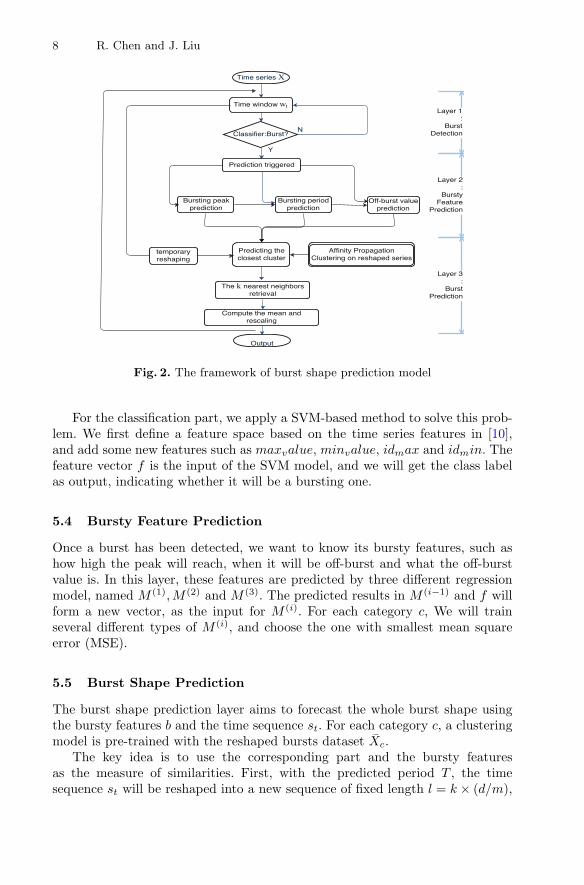
We propose a model framework to predict the entire burst shape of online prod-ucts, shown in Fig. 2. The model has three layers, namely the burst detectionlayer, bursty feature prediction layer, and the burst shape prediction layer. Thefinal layer will generate the output prediction of the whole model. The modelimplements the following work flow:
5.3 Burst Detection
The burst detection layer aims to detect the start of a burst. For time series X,we let the window w slide with the timeline from the start point of X. At timet, we get a sequence st = xt, xt+1, ..., xt+d, and we will use this sequence as theinput of the classification model. The sliding window is to simulate and solvethe real situation in e-commercial websites.
8 R. Chen and J. Liu
Fig. 2. The framework of burst shape prediction model
For the classification part, we apply a SVM-based method to solve this prob-lem. We first define a feature space based on the time series features in [10],and add some new features such as maxvalue, minvalue, idmax and idmin. Thefeature vector f is the input of the SVM model, and we will get the class labelas output, indicating whether it will be a bursting one.
5.4 Bursty Feature Prediction
Once a burst has been detected, we want to know its bursty features, such ashow high the peak will reach, when it will be off-burst and what the off-burstvalue is. In this layer, these features are predicted by three different regressionmodel, named M (1),M (2) and M (3). The predicted results in M (i−1) and f willform a new vector, as the input for M (i). For each category c, We will trainseveral different types of M (i), and choose the one with smallest mean squareerror (MSE).
5.5 Burst Shape Prediction
The burst shape prediction layer aims to forecast the whole burst shape usingthe bursty features b and the time sequence st. For each category c, a clusteringmodel is pre-trained with the reshaped bursts dataset Xc.
The key idea is to use the corresponding part and the bursty featuresas the measure of similarities. First, with the predicted period T , the timesequence st will be reshaped into a new sequence of fixed length l = k × (d/m),
A Novel Framework for Online Sales Burst Prediction 9
s′t = s1, s2, ..., sl. For each cluster center of reshaped bursts x = x1, x2, ..., xm, we
only use the same part x1, x2, ..., xl to calculate the similarity of two sequencesand find the predicted cluster st. There are plenty of methods to measure sim-ilarity, such as Euclidean distance, cosine similarity and so on. For time series,Dynamic Time Warping (DTW) [13] is good alternative, which is designedto find an optimal alignment between two given (time-dependent) sequences.Then, we can find all reshaped bursts in st, and calculate new similaritiesbetween s
′t and their corresponding parts. Here, the new similarity contains
sequence similarity, absolute value of period similarity, peak similarity and off-burst value similarity. The weight of the first part is highest and for otherparts we assign same weights. We choose the highest ranking k sequences,calculate its mean series x
′, and rescale it with the period T as the out-
put prediction. The rescaling method uses the reverse process of reshaping:X = x1, x2, ..., xT , xi = x
′k + (x
′k+1 − x
′k) × (i × m
T − k), k = �i × mT �.
6 Experiments and Evaluation
Setup. For each individual dataset, we randomly divide the samples into threefolds: the training set, the validation set and the test set, with the proportionof 3:1:1. The model is trained using the training set, and is then tested on thevalidation set. Such cross-validation is performed on the same individual datasetfor ten times with random splits, and the reported performance is the averagedvalue cross the ten iterations. Finally we test the model on the test set andreport the performance.
6.1 Evaluation of the Burst Detection Layer
In this layer, we set a maximum number of samples as 30000 to reduce trainingtime, and randomly select the same number of positive and negative samplesfrom the training dataset. Before the training, we evaluate the contributions offeatures with a L1-based linear SVC model, and then reduce the dimensionalityof input feature vector of the classifier, a SVC model with rbf kernel. Precision,Recall and F1-score are reasonable metrics for the evaluation of this layer.
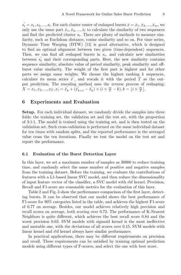
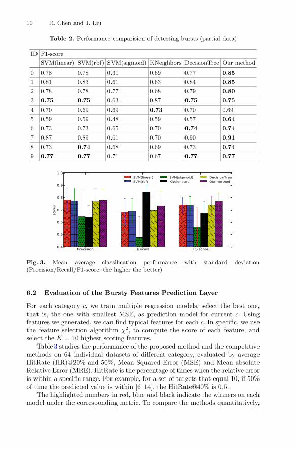
Table 2 and Fig. 3 show the performance comparison of the first layer, detect-ing bursts. It can be observed that our model shows the best performance ofF1-score for 90% categories listed in the table, and achieves the highest F1-scoreof 0.77 on average. Besides, our model achieves relatively high precision andrecall scores on average, both scoring over 0.72. The performance of K-NearestNeighbors is quite different, which achieves the best recall score 0.84 and theworst precision 0.63. SVM models with sigmoid kernel is the most ineffectiveand unstable one, with the deviations of all scores over 0.15. SVM models withlinear kernel and rbf kernel always have similar performance.
In practical applications, there may be different requirements on precisionand recall. These requirements can be satisfied by training optimal predictionmodels using different types of F-scores, and select the one with best score.
10 R. Chen and J. Liu
Table 2. Performance comparision of detecting bursts (partial data)
ID F1-score
SVM(linear) SVM(rbf) SVM(sigmoid) KNeighbors DecisionTree Our method
0 0.78 0.78 0.31 0.69 0.77 0.85
1 0.81 0.83 0.61 0.63 0.84 0.85
2 0.78 0.78 0.77 0.68 0.79 0.80
3 0.75 0.75 0.63 0.87 0.75 0.75
4 0.70 0.69 0.69 0.73 0.70 0.69
5 0.59 0.59 0.48 0.59 0.57 0.64
6 0.73 0.73 0.65 0.70 0.74 0.74
7 0.87 0.89 0.61 0.70 0.90 0.91
8 0.73 0.74 0.68 0.69 0.73 0.74
9 0.77 0.77 0.71 0.67 0.77 0.77
Fig. 3. Mean average classification performance with standard deviation(Precision/Recall/F1-score: the higher the better)
6.2 Evaluation of the Bursty Features Prediction Layer
For each category c, we train multiple regression models, select the best one,that is, the one with smallest MSE, as prediction model for current c. Usingfeatures we generated, we can find typical features for each c. In specific, we usethe feature selection algorithm χ2, to compute the score of each feature, andselect the K = 10 highest scoring features.
Table 3 studies the performance of the proposed method and the competitivemethods on 64 individual datasets of different category, evaluated by averageHitRate (HR)@20% and 50%, Mean Squared Error (MSE) and Mean absoluteRelative Error (MRE). HitRate is the percentage of times when the relative erroris within a specific range. For example, for a set of targets that equal 10, if 50%of time the predicted value is within [6–14], the HitRate@40% is 0.5.
The highlighted numbers in red, blue and black indicate the winners on eachmodel under the corresponding metric. To compare the methods quantitatively,
A Novel Framework for Online Sales Burst Prediction 11
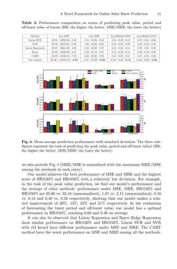
Table 3. Performance comparision on scores of predicting peak value, period andoff-burst value of bursts (HR: the higher the better, MSE/MRE: the lower the better)
Method Avg MSE Avg MRE Avg HitRate@20% Avg HitRate@50%
Linear SVR 29.91—12096.26—3.88 1.91—50.90—0.69 0.14—0.27—0.12 0.37—0.61—0.26
SVR 26.76—10573.25—7.29 1.88—49.65—0.94 0.16—0.27—0.09 0.38—0.61—0.22
Linear Regression 30.95—12861.00—4.98 2.23—62.28—0.57 0.12—0.22—0.14 0.30—0.50—0.30
Bayes 30.22—12399.39—4.97 2.22—61.72—0.57 0.12—0.22—0.14 0.30—0.50—0.30
CART 42.95—15538.12—7.53 2.49—63.28—0.70 0.13—0.25—0.11 0.31—0.54—0.26
Our method 25.66—10032.34—3.78 1.87—47.85—0.56 0.16—0.28—0.15 0.40—0.68—0.38
Fig. 4. Mean average prediction performance with standard deviation. The three sub-figures represent the task of predicting the peak value, period and off-burst value) (HR:the higher the better, MSE/MRE: the lower the better)
we also provide Fig. 4 (MRE/MSE is normalized with the maximum MRE/MSEamong the methods in each entry).
Our model achieves the best performance of MSE and MRE and the highestscore of HR@20% and HR@50% with a relatively low deviation. For example,in the task of the peak value prediction, we find our model’s performance andthe average of other methods’ performance under MSE, MRE, HR@20% andHR@50% are 25.66 vs. 32.16 (unnormalized), 1.87 vs. 2.15 (unnormalized), 0.16vs. 0.13 and 0.40 vs. 0.33 respectively, showing that our model makes a rela-tive improvement of 20%, 13%, 23% and 21% respectively. In the evaluationof forecasting the burst period and off-burst value, our model has a optimalperformance in HR@50%, reaching 0.68 and 0.38 on average.
It can also be observed that Linear Regression and Bayes Ridge Regressionshow similar performance on HR@20% and HR@50%. Linear SVR and SVRwith rbf kernel have different performance under MSE and MRE. The CARTmethod have the worst performance on MSE and MRE among all the methods.
12 R. Chen and J. Liu
6.3 Evaluation of the Burst Shape Prediction Layer
For this prediction task, we compare our model with two different models com-monly used for time series prediction. The metric mean square error (MSE)is used to evaluate the prediction performance. We perform the Affinity Prop-agation Clustering [5] on the dataset of reshaped bursts. Euclidean distanceis applied to calculate the input similarity matrix of the training set, and wechoose DTW distance as the measure of similarity when forecasting. Besides,when the start value of the forecasted result and the last value in the windowdiffer greatly, we apply a decay function to smooth the 30% of the predictedburst series, namely y30%: y = αf + (1 − α)g. Here, we set f as the straight linefrom the last point in the window w to the last point of y30%, and set g as y30%.α is set as the exponential function e(−1/3)t.
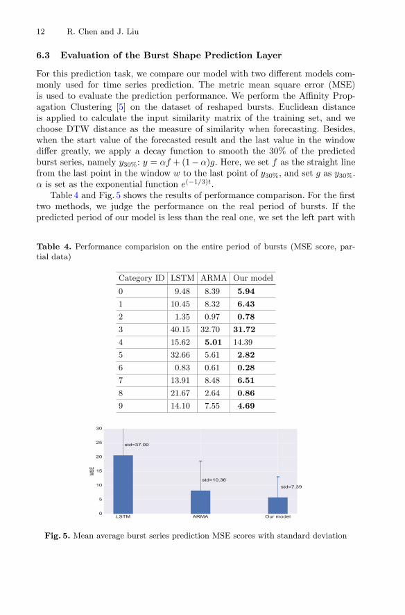
Table 4 and Fig. 5 shows the results of performance comparison. For the firsttwo methods, we judge the performance on the real period of bursts. If thepredicted period of our model is less than the real one, we set the left part with
Table 4. Performance comparision on the entire period of bursts (MSE score, par-tial data)
Category ID LSTM ARMA Our model
0 9.48 8.39 5.94
1 10.45 8.32 6.43
2 1.35 0.97 0.78
3 40.15 32.70 31.72
4 15.62 5.01 14.39
5 32.66 5.61 2.82
6 0.83 0.61 0.28
7 13.91 8.48 6.51
8 21.67 2.64 0.86
9 14.10 7.55 4.69
Fig. 5. Mean average burst series prediction MSE scores with standard deviation
A Novel Framework for Online Sales Burst Prediction 13
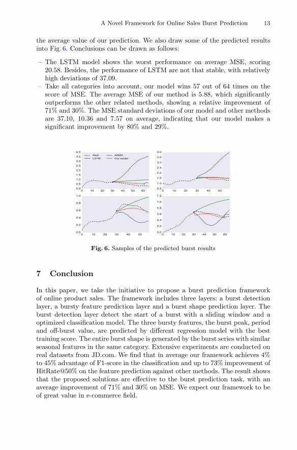
the average value of our prediction. We also draw some of the predicted resultsinto Fig. 6. Conclusions can be drawn as follows:
– The LSTM model shows the worst performance on average MSE, scoring20.58. Besides, the performance of LSTM are not that stable, with relativelyhigh deviations of 37.09.
– Take all categories into account, our model wins 57 out of 64 times on thescore of MSE. The average MSE of our method is 5.88, which significantlyoutperforms the other related methods, showing a relative improvement of71% and 30%. The MSE standard deviations of our model and other methodsare 37.10, 10.36 and 7.57 on average, indicating that our model makes asignificant improvement by 80% and 29%.
Fig. 6. Samples of the predicted burst results
7 Conclusion
In this paper, we take the initiative to propose a burst prediction frameworkof online product sales. The framework includes three layers: a burst detectionlayer, a bursty feature prediction layer and a burst shape prediction layer. Theburst detection layer detect the start of a burst with a sliding window and aoptimized classification model. The three bursty features, the burst peak, periodand off-burst value, are predicted by different regression model with the besttraining score. The entire burst shape is generated by the burst series with similarseasonal features in the same category. Extensive experiments are conducted onreal datasets from JD.com. We find that in average our framework achieves 4%to 45% advantage of F1-score in the classification and up to 73% improvement ofHitRate@50% on the feature prediction against other methods. The result showsthat the proposed solutions are effective to the burst prediction task, with anaverage improvement of 71% and 30% on MSE. We expect our framework to beof great value in e-commerce field.

14 R. Chen and J. Liu
Acknowledgments. This work was supported by the National Natural Science Foun-dation of China (No. 61602487), the Fundamental Research Funds for the Central Uni-versities, and the Research Funds of Renmin University of China (No. 2015030275).
References
1. Agrawal, D., Agrawal, R.P., Singh, J.B., Tripathi, S.P.: E-commerce: true indianpicture. J. Adv. IT 3(4), 250–257 (2012)
2. Avery, S.: Online tool removes costs from process. Purchasing 123(6), 79–81 (1997)3. Barabasi, A.-L.: Bursts: The Hidden Patterns Behind Everything we do, from Your
E-mail to Bloody Crusades. Penguin, New York (2010)4. Cao, L., Zhang, Z.: The 2015 Annual China Electronic Commerce Market Data
Monitoring Report. China Electronic Commerce Research Center, Hangzhou(2016)
5. Frey, B.J., Dueck, D.: Clustering by passing messages between data points. Science315(5814), 972–976 (2007)
6. Gruhl, D., Guha, R., Kumar, R., Novak, J., Tomkins, A.: The predictive powerof online chatter. In: Proceedings of the Eleventh ACM SIGKDD InternationalConference on Knowledge Discovery in Data Mining, pp. 78–87. ACM (2005)
7. Kalman, R.E.: A new approach to linear filtering and prediction problems. Trans.ASME-J. Basic Eng. 82(Series D), 35–45 (1960)
8. Kong, S., Mei, Q., Feng, L., Ye, F., Zhao, Z.: Predicting bursts and popularityof hashtags in real-time. In: Proceedings of the 37th International ACM SIGIRConference on Research and Development in Information Retrieval, pp. 927–930.ACM (2014)
9. Kong, S., Mei, Q., Feng, L., Zhao, Z.: Real-time predicting bursting hashtags onTwitter. In: Li, F., Li, G., Hwang, S., Yao, B., Zhang, Z. (eds.) WAIM 2014.LNCS, vol. 8485, pp. 268–271. Springer, Cham (2014). https://doi.org/10.1007/978-3-319-08010-9 29
10. Kong, S., Mei, Q., Feng, L., Zhao, Z., Ye, F.: On the real-time prediction problemsof bursting hashtags in twitter. arXiv preprint arXiv:1401.2018 (2014)
11. Lin, Y.-R., Margolin, D., Keegan, B., Baronchelli, A., Lazer, D.: # bigbirdsnever die: understanding social dynamics of emergent hashtag. arXiv preprintarXiv:1303.7144 (2013)
12. Ma, Z., Sun, A., Cong, G.: On predicting the popularity of newly emerging hashtagsin Twitter. J. Am. Soc. Inf. Sci. Technol. 64(7), 1399–1410 (2013)
13. Ratanamahatana, C.A., Keogh, E.: Making time-series classification more accu-rate using learned constraints. In: Proceedings of the 2004 SIAM InternationalConference on Data Mining, pp. 11–22. SIAM (2004)
14. Schaidnagel, M., Abele, C., Laux, F., Petrov, I.: Sales prediction with parametrizedtime series analysis. In: Proceedings DBKDA, pp. 166–173 (2013)
15. Thiesing, F.M., Vornberger, O.: Sales forecasting using neural networks. In: 1997International Conference on Neural Networks, vol. 4, pp. 2125–2128. IEEE (1997)
16. Weigend, A.S.: Time Series Prediction: Forecasting the Future and Understandingthe Past. Santa Fe Institute Studies in the Sciences of Complexity (1994)
Analyzing Granger Causality in Climate Datawith Time Series Classification Methods
Christina Papagiannopoulou1(B), Stijn Decubber1, Diego G. Miralles2,3,Matthias Demuzere2, Niko E. C. Verhoest2, and Willem Waegeman1
1 Department of Mathematical Modelling, Statistics and Bioinformatics,Ghent University, Ghent, Belgium
{christina.papagiannopoulou,stijn.decubber,willem.waegeman}@ugent.be2 Laboratory of Hydrology and Water Management,
Ghent University, Ghent, Belgium{matthias.demuzere,niko.verhoest,diego.miralles}@ugent.be
3 Department of Earth Sciences, VU University Amsterdam,Amsterdam, The Netherlands
Abstract. Attribution studies in climate science aim for scientificallyascertaining the influence of climatic variations on natural or anthro-pogenic factors. Many of those studies adopt the concept of Grangercausality to infer statistical cause-effect relationships, while utilizing tra-ditional autoregressive models. In this article, we investigate the potentialof state-of-the-art time series classification techniques to enhance causalinference in climate science. We conduct a comparative experimentalstudy of different types of algorithms on a large test suite that com-prises a unique collection of datasets from the area of climate-vegetationdynamics. The results indicate that specialized time series classificationmethods are able to improve existing inference procedures. Substantialdifferences are observed among the methods that were tested.
Keywords: Climate science · Attribution studies · Causal inferenceGranger causality · Time series classification
1 Introduction
Research questions in climate change research are mostly related to either climateprojection or to climate change attribution. Climate projection or forecasting aimsatpredicting the future state of the climatic system, typically over thenextdecades.The goal of climatic attribution on the other hand is to identify and quantify cause-effect relationships between climate variables andnatural or anthropogenic factors.A well-studied example, both for projection and attribution, is the effect of humangreenhouse gas emissions on global temperature.
The standard approach in the field of climate science is based on simulationstudies with mechanistic climate models, which have been developed, expandedand extensively studied over the last decades. Data-driven models, in contrastto mechanistic models, assume no underlying physical representation of realityc© Springer International Publishing AG 2017Y. Altun et al. (Eds.): ECML PKDD 2017, Part III, LNAI 10536, pp. 15–26, 2017.https://doi.org/10.1007/978-3-319-71273-4_2

16 C. Papagiannopoulou et al.
but directly model the phenomenon of interest by learning a more or less flexiblefunction of some set of input data. Climate science is one of the most data-richresearch domains. With global observations on ever finer spatial and temporalresolutions from both satellite and in-situ measurements, the amount of (publiclyavailable) climatic data sets has vastly grown over the last decades. It goeswithout any doubt that there is a big potential for making progress in climatescience with advanced machine learning models.
The most common data-driven approach for identifying causal relationshipsin climate science consists of Granger causality modelling [17]. Analyses of thiskind have been applied to investigate the influence of one climatic variable onanother, e.g., the Granger causal effect of CO2 on global temperature [1,20], ofvegetation and snow coverage on temperature [19], of sea surface temperatureson the North Atlantic Oscillation [26], or of the El Nino Southern Oscillation onthe Indian monsoon [25]. In Granger causality studies, one assumes that a timeseries A Granger-causes a time series B, if the past of A is helpful in predictingthe future of B. The underlying predictive model that is commonly consideredin such a context is a linear vector autoregressive model [8,32]. Similar to otherstatistical inference procedures, conclusions are only valid as long as all potentialconfounders are incorporated in the analysis. The concept of Granger-causalitywill be reviewed in Sect. 2.
In recent work, we have shown that causal inference in climate science can besubstantially improved by replacing traditional statistical models with non-linearautoregressive methods that incorporate hand-crafted higher-level features of rawtime series [27]. However, approaches of that kind require a lot of domain knowl-edge about the working of our planet. Moreover, higher-level features that areincluded in the models often originate from rather arbitrary decisions. In this arti-cle, we postulate that causal inference in climate science can be further improvedby using automated feature construction methods for time series. In recent years,methods of that kind have shown to yield substantial performance gains in thearea of time series classification. However, we believe that some of those methodsalso have a lot of potential to improve causal inference in climate science, and thegoal of this paper is to provide experimental evidence for that. We experimentallycompare a large number of time series classification methods – an overview andmore discussion of these methods will be given in Sect. 3.
Most attribution studies in climate science infer causal relationships betweentime series of continuous measurements, leading to regression settings. However,classification settings arise when targeting extreme events, such as heatwaves,droughts or floods. We will conduct an experimental study in the area of investi-gating climate-vegetation dynamics, where such a classification setting naturallyarises. This is an interesting application domain for testing time series classifica-tion methods, due to the availability of large and complex datasets with worldwidecoverage. It is also a practically-relevant setting, because extremes in vegetationcan reveal the vulnerability of ecosystems w.r.t. climate change [23]. A more pre-cise description of this application domain and the experimental setup will be pro-vided in Sect. 4. In Sect. 5, we will present the main results, which will allow us to

Analyzing Granger Causality with Time Series Classification Methods 17
formulate conclusions concerning which methods are more appropriate in the areaof climate sciences.
2 Granger Causality for Attribution in Climate Science
Granger causality [17] can be seen as a predictive notion of causality betweentime series. In the bivariate case, when two time series are considered, one com-pares the forecasts of two models; a baseline model that includes only informa-tion from the target time series (which resembles the effect) and a so-called fullmodel that includes also the history of the second time series (which resemblesthe cause). Given two time series x = [x1, x2, ..., xN ] and y = [y1, y2, ..., yN ], withN being the length of the time series, one says that the time series x Granger-causes the time series y if the forecast of y at a specific time stamp t improveswhen information of the history of x is included in the model.
In this paper we will limit our analysis to situations where the target timeseries y consists of {0, 1}-measurements that denote the presence or absenceof an extreme event at time stamp t. As such, one ends up with solving twoclassification problems, one for the baseline and one for the full model. We willwork with the Area Under the Curve (AUC) as performance measure, becausethe class distribution will be heavily imbalanced, as a natural result of modellingextreme events. Let y denote the new time series that originates as the one-stepahead forecast of y using either the baseline or the full model, then Grangercausality can be formally formulated as follows:
Definition 1. A time series x Granger-causes y if AUC(y, y) increases whenxt−1, xt−2, ..., xt−P are considered for predicting yt, in contrast to consideringyt−1, yt−2, ..., yt−P only, where P is the lag-time moving window.
Granger causality studies might yield incorrect conclusions when additional(confounding) effects exerted by other climatic or environmental variables arenot taken into account [13]. The problem can be mitigated by considering timeseries of additional variables. For example, let us assume one has observed a thirdvariable w, which might act as a confounder in deciding whether x Granger-causes y. The above definition then naturally extends as follows.
Definition 2. We say that time series x Granger-causes y conditioned ontime series w if AUC(y, y) increases when xt−1, xt−2, ..., xt−P are includedin the prediction of yt, in contrast to considering yt−1, yt−2, ..., yt−P andwt−1, wt−2, ..., wt−P only, where P is the lag-time moving window.
An extension to more than three time series is straightforward. In our exper-iments, y will represent the vegetation extremes at a given location, whereasx and w can be the time series of any climatic variable at that location (e.g.,temperature, precipitation or radiation).
Generally, the null hypothesis (H0) of Granger causality is that the base-line model has equal prediction error as the full model. Alternatively, if thefull model predicts the target variable y significantly better than the baseline
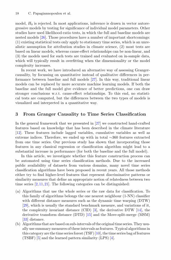
18 C. Papagiannopoulou et al.
model, H0 is rejected. In most applications, inference is drawn in vector autore-gressive models by testing for significance of individual model parameters. Otherstudies have used likelihood-ratio tests, in which the full and baseline models arenested models [26]. Those procedures have a number of important shortcomings:(1) existing statistical tests only apply to stationary time series, which is an unre-alistic assumption for attribution studies in climate science, (2) most tests arebased on linear models, whereas cause-effect relationships can be non-linear, and(3) the models used for such tests are trained and evaluated on in-sample data,which will typically result in overfitting when the dimensionality or the modelcomplexity increases.
In recent work, we have introduced an alternative way of assessing Granger-causality, by focussing on quantitative instead of qualitative differences in per-formance between baseline and full models [27]. In this way, traditional linearmodels can be replaced by more accurate machine learning models. If both thebaseline and the full model give evidence of better predictions, one can drawstronger conclusions w.r.t. cause-effect relationships. To this end, no statisti-cal tests are computed, but the differences between the two types of models isvisualized and interpreted in a quantitative way.
3 From Granger Causality to Time Series Classification
In the general framework that we presented in [27] we constructed hand-craftedfeatures based on knowledge that has been described in the climate literature[12]. These features include lagged variables, cumulative variables as well asextreme indices. Therefore, we ended up with in total ∼360 features extractedfrom one time series. Our previous study has shown that incorporating thosefeatures in any classical regression or classification algorithm might lead to asubstantial increase in performance (for both the baseline and the full model).
In this article, we investigate whether this feature construction process canbe automated using time series classification methods. Due to the increasedpublic availability of datasets from various domains, many novel time seriesclassification algorithms have been proposed in recent years. All those methodseither try to find higher-level features that represent discriminative patterns orsimilarity measures that define an appropriate notion of relatedness between twotime series [2,11,21]. The following categories can be distinguished:
(a) Algorithms that use the whole series or the raw data for classification. Tothis family of algorithms belongs the one nearest neighbour (1-NN) classifierwith different distance measures such as the dynamic time warping (DTW)[29], which is usually the standard benchmark measure, and variations of it,the complexity invariant distance (CID) [3], the derivative DTW [14], thederivative transform distance (DTD) [15] and the Move-split-merge (MSM)[33] distance.
(b) Algorithms that arebasedon sub-intervals of the original time series.Theyusu-ally use summary measures of these intervals as features. Typical algorithms inthis category are the time series forest (TSF) [10], the time series bag of features(TSBF) [5] and the learned pattern similarity (LPS) [4].

Analyzing Granger Causality with Time Series Classification Methods 19
(c) Algorithms that are attempting to find informative patterns, called shapelets,in thedata.An informative shapelet is apattern thathelps indistinguishing theclasses by its presence or absence. Representative algorithms of this class arethe Fast shapelets (FS) [28], the Shapelet transform (ST) [18] and the Learnedshapelets (LS) [16].
(d) Algorithms that are based on the frequency of the patterns in a time series.These algorithms build a vocabulary of patterns and form a histogram foreach observation by using this vocabulary. Algorithms such as the Bag ofpatterns (BOP) [22], the Symbolic aggregate approximation-vector spacemodel (SAXVSM) [31] and the Bag of SFA symbols (BOSS) [30] are basedon the idea of a pattern vocabulary.
(e) Finally, there are approaches that combine more than one from the abovetechniques, forming ensemble models. A recently proposed algorithm namedCollection of transformation ensembles (COTE) combines a large number ofclassifiers constructed in the time, frequency, and shapelet transformationdomains.
In our comparative study, we run algorithms from the first four differentgroups. The main criteria for including a particular algorithm in our analysis are(1) availability of source code, (2) running time for the datasets that we consider,and (3) interpretability of the extracted features. Since we have collected multipletime series for a large part of the world (3,536 locations in total), the algorithmsshould run in a reasonable amount of time. Several algorithms had problems tofinish within 3 days.
4 Experimental Setup
In order to evaluate the above-mentioned time series classification methods forcausal inference, we adopt an experimental setup that is similar to [27]. Thenon-linear Granger causality framework is adopted to explore the influence ofpast-time climate variability on vegetation dynamics. To this end, data sets ofobservational nature were collected to construct climatic time series that arethen used to predict vegetation extremes. Data sets have been selected on thebasis of meeting the following requirements: (a) an expected relevance of thevariable for vegetation dynamics, (b) the availability of multi-decadal records,and (c) the availability of an adequate spatial and daily temporal resolution. Inour previous work, we collected in this way in total 21 datasets. For the presentstudy, we retained three of them, while covering the three basic climatic vari-ables: water availability, temperature, and radiation. The main reason for makingthis restriction was that in that way the running time of the different time seriesclassification algorithms could be substantially reduced. Specifically, we collectedone precipitation dataset, which is coming from a combination of in-situ, satellitedata, and reanalysis outputs, called Multi-Source Weighted-Ensemble Precipita-tion (MSWEP) [7]. We include one temperature dataset, which is a reanalysisdata set, and one radiation dataset from the European Centre for Medium-RangeWeather Forecasts (ECMWF) ERA-Interim [9].

20 C. Papagiannopoulou et al.
In addition to those three climatic datasets, we also collected a vegeta-tion dataset. We use the satellite-based Normalized Difference Vegetation Index(NDVI) [34], which is a commonly used monthly long-term global indicator ofvegetation [6]. Roughly speaking, NDVI is a graphical greenness indicator whichmeasures how green is a specific point on the Earth at a specific time stamp.The study period starting from 1981–2010 is set by the length of the NDVIrecord. The dataset is converted to a 1◦ spatial resolution to match with theclimatic datasets.
For most locations on Earth, NDVI time series exhibit a clear seasonal cycleand trend – see top panel of Fig. 1 for a representative example. However, in cli-mate science, the interesting part of such a time series is the residual component,usually referred to as seasonal anomalies. In a statistical sense, climatic data canonly be useful to predict this residual component, as both the seasonal cycle andthe trend can be modelled with pure autoregressive features. Similarly as in [27],we isolate the residual component using time series decomposition methods, andwe work further with this residual component – see bottom panel of Fig. 1 for anillustration. In a next step, extremes are obtained from the residuals, while tak-ing the spatial distribution of those extremes into account. The most straightfor-ward way is setting a fixed threshold per location, such as the 10% percentile ofthe residuals. However, this leads to spatial distributions that are physically notplausible, because one cannot expect that the same number of vegetation extremesis observed in all locations on Earth. At some locations, vegetation extremes aremore probable to happen. For this reason, we group the location pixels into areaswith the same vegetation type, by using the global vegetation classification schemeof the International Geosphere-Biosphere Program (IGBP) [24], which is generi-cally used throughout a range of communities. We selected the map of the year2001 (closer to the middle of our period of interest). In order to end up withcoherent regions that have similar climatic and vegetation characteristics, we fur-ther divided the vegetation groups into areas in which only neighboring pixelscan belong to the same group. That way, we create 27 different pixel groups inAmerica, see Fig. 2. We limit the study to America because some of the time seriesclassification methods that we analyse have a long running time. Once we knowwhich of those methods perform well, the study can of course be further extendedto other regions, under the assumption that the same methods are favored forthose regions.
The vegetation extremes are then defined by applying a 10th percentilethreshold on the seasonal anomalies of each region. This is a common thresh-old in defining extremes in vegetation [35]. Applying a lower threshold wouldresult in extreme events that are extremely rare, making it impossible to trainpredictive models. In this way, we produce the target variable of our time seriesclassification task. The presence of an extreme is denoted with a ‘1’ and theabsence with a ‘0’. Unsurprisingly, the distribution of the vegetation extremes intime indicates that many more extremes occur in recent years, which meansthat a clear trend appears again in the time series of extreme events, eventhough the initial time series was detrended. This makes the time series highly
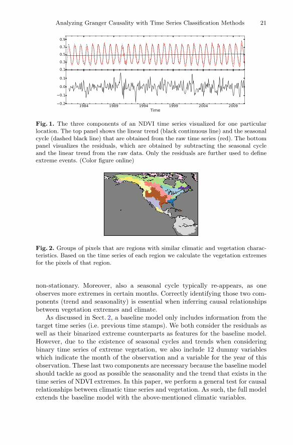
Analyzing Granger Causality with Time Series Classification Methods 21
Fig. 1. The three components of an NDVI time series visualized for one particularlocation. The top panel shows the linear trend (black continuous line) and the seasonalcycle (dashed black line) that are obtained from the raw time series (red). The bottompanel visualizes the residuals, which are obtained by subtracting the seasonal cycleand the linear trend from the raw data. Only the residuals are further used to defineextreme events. (Color figure online)
Fig. 2. Groups of pixels that are regions with similar climatic and vegetation charac-teristics. Based on the time series of each region we calculate the vegetation extremesfor the pixels of that region.
non-stationary. Moreover, also a seasonal cycle typically re-appears, as oneobserves more extremes in certain months. Correctly identifying those two com-ponents (trend and seasonality) is essential when inferring causal relationshipsbetween vegetation extremes and climate.
As discussed in Sect. 2, a baseline model only includes information from thetarget time series (i.e. previous time stamps). We both consider the residuals aswell as their binarized extreme counterparts as features for the baseline model.However, due to the existence of seasonal cycles and trends when consideringbinary time series of extreme vegetation, we also include 12 dummy variableswhich indicate the month of the observation and a variable for the year of thisobservation. These last two components are necessary because the baseline modelshould tackle as good as possible the seasonality and the trend that exists in thetime series of NDVI extremes. In this paper, we perform a general test for causalrelationships between climatic time series and vegetation. As such, the full modelextends the baseline model with the above-mentioned climatic variables.
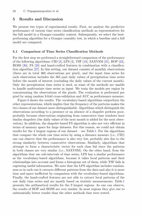
22 C. Papagiannopoulou et al.
5 Results and Discussion
We present two types of experimental results. First, we analyze the predictiveperformance of various time series classification methods as representatives forthe full model in a Granger-causality context. Subsequently, we select the best-performing algorithm for a Granger causality test, in which a baseline and a fullmodel are compared.
5.1 Comparison of Time Series Classification Methods
For the first step we performed a straightforward comparison of the performanceof the following algorithms: CID [3], LPS [4], TSF [10], SAXVSM [31], BOP [22],BOSS [30], FS [28] and hand-crafted features in combination with a classifica-tion algorithm [27]. In this setting, our dataset consists of monthly observations(there are in total 360 observations per pixel), and the input time series foreach observation includes the 365 past daily values of precipitation time seriesbefore the month of interest (excluding the daily values of the current month).Only the precipitation time series is used, as some of the methods are unableto handle multivariate time series as input. We train the models per region byconcatenating the observations of the pixels. The evaluation is performed perpixel by using random 3-fold cross-validation and AUC as performance measure.
Figure 3 shows the results. The vocabulary-based algorithms outperform theother representations, which implies that the frequency of the patterns makes thetwo classes of our dataset more distinguishable. Algorithms which distinguish theobservations according to a presence or an absence of a shapelet perform poor,probably because observations originating from consecutive time windows havesimilar shapelets (the daily values of the next month is added for the next obser-vation). In addition, the shapelet-based FS algorithm is also not very efficient interms of memory space for large datasets. For this reason, we could not obtainresults for the 4 largest regions of our dataset – see Table 1. For the algorithmsthat compare the whole raw time series by using a distance measure (i.e., CID)one can observe that the performance is also very low, probably also due to thestrong similarity between consecutive observations. Similarly, algorithms thatattempt to form a characteristic vector for each class fail since the patternsin both classes are very similar (i.e., SAXVSM). On the other hand, from thealgorithms that use sub-intervals of time series, LPS has a similar performanceas the vocabulary-based algorithms, because it takes local patterns and theirrelationships into account and forms a histogram out of them, while TSF fails incapturing useful information. We note that the LPS algorithm includes random-ness so in each run it extracts different patterns from the data and also it is moretime and space inefficient by comparison with the vocabulary-based algorithms.Finally, the hand-crafted features are not able to extract local patterns of theraw daily time series and are mostly based on statistic measurements. Table 1presents the arithmetical results for the 9 largest regions. As one can observe,the results of BOP and BOSS are very similar. In most regions they give rise tosubstantially better results than the other methods that were tested.
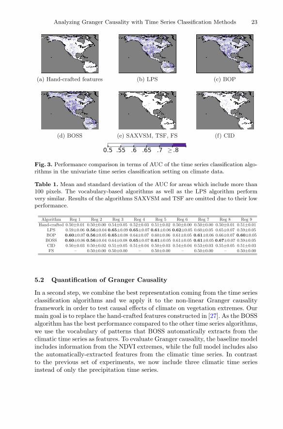
Analyzing Granger Causality with Time Series Classification Methods 23
Fig. 3. Performance comparison in terms of AUC of the time series classification algo-rithms in the univariate time series classification setting on climate data.
Table 1. Mean and standard deviation of the AUC for areas which include more than100 pixels. The vocabulary-based algorithms as well as the LPS algorithm performvery similar. Results of the algorithms SAXVSM and TSF are omitted due to their lowperformance.
Algorithm Reg 1 Reg 2 Reg 3 Reg 4 Reg 5 Reg 6 Reg 7 Reg 8 Reg 9
Hand-crafted 0.50±0.01 0.50±0.00 0.54±0.05 0.52±0.03 0.51±0.02 0.50±0.00 0.50±0.00 0.50±0.01 0.51±0.01LPS 0.59±0.06 0.56±0.04 0.65±0.09 0.65±0.07 0.61±0.06 0.62±0.05 0.60±0.05 0.65±0.07 0.59±0.05BOP 0.60±0.07 0.56±0.05 0.65±0.08 0.64±0.07 0.60±0.06 0.61±0.05 0.61±0.06 0.66±0.07 0.60±0.05BOSS 0.60±0.06 0.56±0.04 0.64±0.08 0.65±0.07 0.61±0.05 0.61±0.05 0.61±0.05 0.67±0.07 0.59±0.05CID 0.50±0.03 0.50±0.02 0.51±0.05 0.51±0.04 0.50±0.03 0.54±0.04 0.53±0.03 0.55±0.05 0.51±0.03
±0.00 0.50± ± ±FS – 0.50 0.00 – 0.50 0.00 – 0.50 0.00 – 0.50±0.00
5.2 Quantification of Granger Causality
In a second step, we combine the best representation coming from the time seriesclassification algorithms and we apply it to the non-linear Granger causalityframework in order to test causal effects of climate on vegetation extremes. Ourmain goal is to replace the hand-crafted features constructed in [27]. As the BOSSalgorithm has the best performance compared to the other time series algorithms,we use the vocabulary of patterns that BOSS automatically extracts from theclimatic time series as features. To evaluate Granger causality, the baseline modelincludes information from the NDVI extremes, while the full model includes alsothe automatically-extracted features from the climatic time series. In contrastto the previous set of experiments, we now include three climatic time seriesinstead of only the precipitation time series.
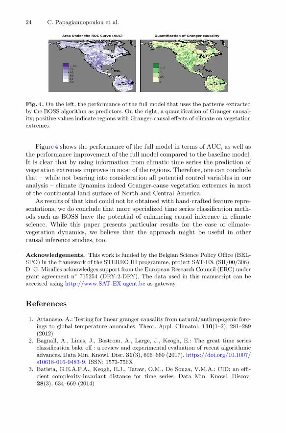
24 C. Papagiannopoulou et al.
Fig. 4. On the left, the performance of the full model that uses the patterns extractedby the BOSS algorithm as predictors. On the right, a quantification of Granger causal-ity; positive values indicate regions with Granger-causal effects of climate on vegetationextremes.
Figure 4 shows the performance of the full model in terms of AUC, as well asthe performance improvement of the full model compared to the baseline model.It is clear that by using information from climatic time series the prediction ofvegetation extremes improves in most of the regions. Therefore, one can concludethat – while not bearing into consideration all potential control variables in ouranalysis – climate dynamics indeed Granger-cause vegetation extremes in mostof the continental land surface of North and Central America.
As results of that kind could not be obtained with hand-crafted feature repre-sentations, we do conclude that more specialized time series classification meth-ods such as BOSS have the potential of enhancing causal inference in climatescience. While this paper presents particular results for the case of climate-vegetation dynamics, we believe that the approach might be useful in othercausal inference studies, too.
Acknowledgements. This work is funded by the Belgian Science Policy Office (BEL-SPO) in the framework of the STEREO III programme, project SAT-EX (SR/00/306).D. G. Miralles acknowledges support from the European Research Council (ERC) undergrant agreement n◦ 715254 (DRY-2-DRY). The data used in this manuscript can beaccessed using http://www.SAT-EX.ugent.be as gateway.
References
1. Attanasio, A.: Testing for linear granger causality from natural/anthropogenic forc-ings to global temperature anomalies. Theor. Appl. Climatol. 110(1–2), 281–289(2012)
2. Bagnall, A., Lines, J., Bostrom, A., Large, J., Keogh, E.: The great time seriesclassification bake off : a review and experimental evaluation of recent algorithmicadvances. Data Min. Knowl. Disc. 31(3), 606–660 (2017). https://doi.org/10.1007/s10618-016-0483-9. ISSN: 1573-756X
3. Batista, G.E.A.P.A., Keogh, E.J., Tataw, O.M., De Souza, V.M.A.: CID: an effi-cient complexity-invariant distance for time series. Data Min. Knowl. Discov.28(3), 634–669 (2014)
Analyzing Granger Causality with Time Series Classification Methods 25
4. Baydogan, M.G., Runger, G.: Time series representation and similarity based onlocal autopatterns. Data Min. Knowl. Discov. 30(2), 476–509 (2016)
5. Baydogan, M.G., Runger, G., Tuv, E.: A bag-of-features framework to classify timeseries. IEEE Trans. Patt. Anal. Mach. Intell. 35(11), 2796–2802 (2013)
6. Beck, H.E., McVicar, T.R., van Dijk, A.I.J.M., Schellekens, J., de Jeu, R.A.M.,Bruijnzeel, L.A.: Global evaluation of four AVHRR-NDVI data sets: intercom-parison and assessment against landsat imagery. Remote Sens. Environ. 115(10),2547–2563 (2011)
7. Beck, H.E., van Dijk, A.I.J.M., Levizzani, V., Schellekens, J., Miralles, D.G.,Martens, B., de Roo, A.: MSWEP: 3-hourly 0.25◦ global gridded precipitation(1979–2015) by merging gauge, satellite, and reanalysis data. Hydrol. Earth Syst.Sci. Discuss. 2016, 1–38 (2016)
8. Chapman, D., Cane, M.A., Henderson, N., Lee, D.E., Chen, C.: A vector autore-gressive ENSO prediction model. J. Clim. 28(21), 8511–8520 (2015)
9. Dee, D.P., Uppala, S.M., Simmons, A.J., Berrisford, P., Poli, P., Kobayashi, S.,Andrae, U., Balmaseda, M.A., Balsamo, G., Bauer, P., et al.: The ERA-Interimreanalysis: configuration and performance of the data assimilation system. Q. J.Royal Meteorol. Soc. 137(656), 553–597 (2011)
10. Deng, H., Runger, G., Tuv, E., Vladimir, M.: A time series forest for classificationand feature extraction. Inf. Sci. 239, 142–153 (2013)
11. Ding, H., Trajcevski, G., Scheuermann, P., Wang, X., Keogh, E.: Querying andmining of time series data: experimental comparison of representations and dis-tance measures. Proc. VLDB Endowment 1(2), 1542–1552 (2008)
12. Donat, M.G., Alexander, L.V., Yang, H., Durre, I., Vose, R., Dunn, R.J.H., Willett,K.M., Aguilar, E., Brunet, M., Caesar, J., et al.: Updated analyses of temperatureand precipitation extreme indices since the beginning of the twentieth century: theHadEX2 dataset. J. Geophys. Res.: Atmos. 118(5), 2098–2118 (2013)
13. Geiger, P., Zhang, K., Gong, M., Janzing, D., Scholkopf, B.: Causal inferenceby identification of vector autoregressive processes with hidden components. InProceedings of 32th International Conference on Machine Learning (ICML 2015)(2015)
14. Gorecki, T., �Luczak, M.: Using derivatives in time series classification. Data Min.Knowl. Disc. 26(2), 310–331 (2013). https://doi.org/10.1007/s10618-012-0251-4.ISSN: 1573-756X
15. Gorecki, T., �Luczak, M.: Non-isometric transforms in time series classification usingDTW. Knowl.-Based Syst. 61, 98–108 (2014)
16. Grabocka, J., Schilling, N., Wistuba, M., Schmidt-Thieme, L.: Learning time-seriesshapelets. In: Proceedings of the 20th ACM SIGKDD International Conference onKnowledge Discovery and Data Mining, pp. 392–401. ACM (2014)
17. Granger, C.W.J.: Investigating causal relations by econometric models and cross-spectral methods. Econometrica: J. Econ. Soc. 37, 424–438 (1969)
18. Hills, J., Lines, J., Baranauskas, E., Mapp, J., Bagnall, A.: Classification of timeseries by shapelet transformation. Data Min. Knowl. Discov. 28(4), 851–881 (2014)
19. Kaufmann, R.K., Zhou, L., Myneni, R.B., Tucker, C.J., Slayback, D., Shabanov,N.V., Pinzon, J.: The effect of vegetation on surface temperature: a statisticalanalysis of NDVI and climate data. Geophys. Res. Lett. 30(22) (2003)
20. Kodra, E., Chatterjee, S., Ganguly, A.R.: Exploring granger causality betweenglobal average observed time series of carbon dioxide and temperature. Theor.Appl. Climatol. 104(3–4), 325–335 (2011)
21. Liao, T.W.: Clustering of time series data a survey. Patt. Recogn. 38(11), 1857–1874 (2005)

26 C. Papagiannopoulou et al.
22. Lin, J., Khade, R., Li, Y.: Rotation-invariant similarity in time series using bag-of-patterns representation. J. Intell. Inf. Syst. 39(2), 287–315 (2012)
23. Liu, G., Liu, H., Yin, Y.: Global patterns of NDVI-indicated vegetation extremesand their sensitivity to climate extremes. Environ. Res. Lett. 8(2), 025009 (2013)
24. Loveland, T.R., Belward, A.S.: The IGBP-DIS global 1km land cover data set,discover: first results. Int. J. Remote Sens. 18(15), 3289–3295 (1997)
25. Mokhov, I.I., Smirnov, D.A., Nakonechny, P.I., Kozlenko, S.S., Seleznev, E.P.,Kurths, J.: Alternating mutual influence of El-Nino/southern oscillation and Indianmonsoon. Geophys. Res. Lett. 38(8) (2011)
26. Mosedale, T.J., Stephenson, D.B., Collins, M., Mills, T.C.: Granger causality ofcoupled climate processes: ocean feedback on the North Atlantic Oscillation. J.Clim. 19(7), 1182–1194 (2006)
27. Papagiannopoulou, C., Miralles, D.G., Verhoest, N.E.C., Dorigo, W.A., Waege-man, W.: A non-linear Granger causality framework to investigate climate-vegetation dynamics. Geosci. Model Dev. 10, 1–24 (2017)
28. Rakthanmanon, T., Keogh, E.: Fast shapelets: a scalable algorithm for discoveringtime series shapelets. In: Proceedings of the 2013 SIAM International Conferenceon Data Mining, pp. 668–676. SIAM (2013)
29. Sakoe, H., Chiba, S.: Dynamic programming algorithm optimization for spokenword recognition. IEEE Trans. Acoust. Speech Sig. Process. 26(1), 43–49 (1978)
30. Schafer, P.: The BOSS is concerned with time series classification in the presenceof noise. Data Min. Knowl. Discov. 29(6), 1505–1530 (2015)
31. Senin, P., Malinchik, S.: SAX-VSM: interpretable time series classification usingsax and vector space model. In: 2013 IEEE 13th International Conference on DataMining (ICDM), pp. 1175–1180. IEEE (2013)
32. Shahin, M.A., Ali, M.A., Ali, A.B.M.S.: Vector Autoregression (VAR) modelingand forecasting of temperature, humidity, and cloud coverage. In: Islam, T., Srivas-tava, P.K., Gupta, M., Zhu, X., Mukherjee, S. (eds.) Computational IntelligenceTechniques in Earth and Environmental Sciences, pp. 29–51. Springer, Dordrecht(2014). https://doi.org/10.1007/978-94-017-8642-3 2
33. Stefan, A., Athitsos, V., Das, G.: The move-split-merge metric for time series.IEEE Trans. Knowl. Data Eng. 25(6), 1425–1438 (2013)
34. Tucker, C.J., Pinzon, J.E., Brown, M.E., Slayback, D.A., Pak, E.W., Mahoney, R.,Vermote, E.F., El Saleous, N.: An extended AVHRR 8-km NDVI dataset compat-ible with MODIS and SPOT vegetation NDVI data. Int. J. Remote Sens. 26(20),4485–4498 (2005)
35. Zscheischler, J., Mahecha, M.D., Harmeling, S., Reichstein, M.: Detection and attri-bution of large spatiotemporal extreme events in Earth observation data. Ecol.Inform. 15, 66–73 (2013)
Automatic Detection and Recognitionof Individuals in Patterned Species
Gullal Singh Cheema(B) and Saket Anand
IIIT-Delhi, New Delhi, India{gullal1408,anands}@iiitd.ac.in
Abstract. Visual animal biometrics is rapidly gaining popularity as itenables a non-invasive and cost-effective approach for wildlife monitoringapplications. Widespread usage of camera traps has led to large volumesof collected images, making manual processing of visual content hard tomanage. In this work, we develop a framework for automatic detectionand recognition of individuals in different patterned species like tigers,zebras and jaguars. Most existing systems primarily rely on manual inputfor localizing the animal, which does not scale well to large datasets.In order to automate the detection process while retaining robustnessto blur, partial occlusion, illumination and pose variations, we use therecently proposed Faster-RCNN object detection framework to efficientlydetect animals in images. We further extract features from AlexNet ofthe animal’s flank and train a logistic regression (or Linear SVM) clas-sifier to recognize the individuals. We primarily test and evaluate ourframework on a camera trap tiger image dataset that contains imagesthat vary in overall image quality, animal pose, scale and lighting. Wealso evaluate our recognition system on zebra and jaguar images to showgeneralization to other patterned species. Our framework gives perfectdetection results in camera trapped tiger images and a similar or betterindividual recognition performance when compared with state-of-the-artrecognition techniques.
Keywords: Animal biometrics · Wildlife monitoringDetection · Recognition · Convolutional neural networkComputer vision
1 Introduction
Over the past two decades, advances in visual pattern recognition have ledto many efficient visual biometric systems for identifying human individualsthrough various modalities like iris images [7,27], facial images [1,28] and finger-prints [13,14]. Since the identification process relies on visual pattern matching,it is convenient and minimally invasive, which in turn makes it amenable to usewith non-cooperative subjects as well. Consequently, visual biometrics has beenapplied to wild animals, where non-invasive techniques provide a huge advantage
c© Springer International Publishing AG 2017Y. Altun et al. (Eds.): ECML PKDD 2017, Part III, LNAI 10536, pp. 27–38, 2017.https://doi.org/10.1007/978-3-319-71273-4_3
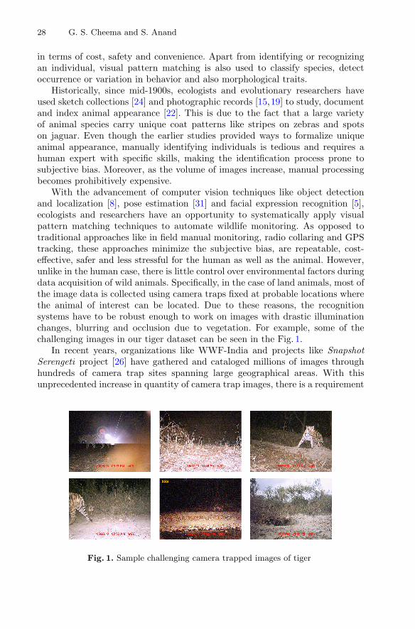
28 G. S. Cheema and S. Anand
in terms of cost, safety and convenience. Apart from identifying or recognizingan individual, visual pattern matching is also used to classify species, detectoccurrence or variation in behavior and also morphological traits.
Historically, since mid-1900s, ecologists and evolutionary researchers haveused sketch collections [24] and photographic records [15,19] to study, documentand index animal appearance [22]. This is due to the fact that a large varietyof animal species carry unique coat patterns like stripes on zebras and spotson jaguar. Even though the earlier studies provided ways to formalize uniqueanimal appearance, manually identifying individuals is tedious and requires ahuman expert with specific skills, making the identification process prone tosubjective bias. Moreover, as the volume of images increase, manual processingbecomes prohibitively expensive.
With the advancement of computer vision techniques like object detectionand localization [8], pose estimation [31] and facial expression recognition [5],ecologists and researchers have an opportunity to systematically apply visualpattern matching techniques to automate wildlife monitoring. As opposed totraditional approaches like in field manual monitoring, radio collaring and GPStracking, these approaches minimize the subjective bias, are repeatable, cost-effective, safer and less stressful for the human as well as the animal. However,unlike in the human case, there is little control over environmental factors duringdata acquisition of wild animals. Specifically, in the case of land animals, most ofthe image data is collected using camera traps fixed at probable locations wherethe animal of interest can be located. Due to these reasons, the recognitionsystems have to be robust enough to work on images with drastic illuminationchanges, blurring and occlusion due to vegetation. For example, some of thechallenging images in our tiger dataset can be seen in the Fig. 1.
In recent years, organizations like WWF-India and projects like SnapshotSerengeti project [26] have gathered and cataloged millions of images throughhundreds of camera trap sites spanning large geographical areas. With thisunprecedented increase in quantity of camera trap images, there is a requirement
Fig. 1. Sample challenging camera trapped images of tiger

Automatic Detection and Recognition of Individuals in Patterned Species 29
of visual monitoring systems that can automatically sort and organize imagesbased on a desired category (species/individual level) in short amount of time.Also, many of the animal species are endangered and require continuous moni-toring, especially in areas where they are vulnerable to poaching, predators andalready less in number. Such monitoring efforts can help to protect animals, main-tain population across different geographical areas and also protect the localecosystem.
In this work, we develop a framework for detecting and recognizing individ-ual patterned species that have unique coat patterns such as stripes on zebras,tigers and spots on Jaguars. State-of-the-art systems such as Extract-Compare[12] by Hiby et al. and HotSpotter [6] by Crall et al. work well, but require userinput for every image and hence fail to scale to large datasets. Automatic detec-tion methods proposed in [3,4] detect smaller patches on animals but not thecomplete animal, and are sensitive to lighting conditions and multiple instancesof animals in the same image. In this work, we use the recently proposed convo-lutional neural network (CNN) based detector, Faster-RCNN [23] by Ren et al.that is able to detect different objects at multiple scales. The advantage of usinga deep CNN based architecture is robustness to illumination and pose variationsas well as location invariance, which proves to be very effective for localizinganimals in images in uncontrolled environments. We use Faster-RCNN to detectthe body and flank region of the animal and pass it through a pre-trainedAlexNet [16] to extract discriminatory features, which is used by a logistic regres-sion classifier for individual recognition.
The remainder of the paper is structured as follows. In Sect. 2, we willbriefly talk about recent related work in animal detection and individual animalrecognition. Section 3 lays the groundwork for the description of our proposedframework in Sect. 4. We then present empirical results on data sets of variouspatterned species, and report performance comparisons in Sect. 5 before con-cluding in Sect. 6.
2 Related Work
In this section we briefly discuss recent advances in animal species and individualidentification, focusing on land animals exhibiting unique coat patterns.
2.1 Animal Detection
One of the earliest works on automatic animal detection [3,4] uses Haar-likefeatures and a low-level feature tracker to detect a lion’s face and extract infor-mation to predict its activity like still, walking or trotting. The system works inreal time and is able to detect faces at multiple scales although only with slightpose variations. Zhang et al. [30] detect heads of animals like tiger, cat, dog,cheetah, etc. by using shape and texture features to improve image retrieval.The approach relies on prominent ‘pointed’ ear shapes in frontal poses whichmakes it sensitive to head-pose variations. These approaches rely on identifying

30 G. S. Cheema and S. Anand
different parts of the animal to detect and track an individual, but are likely tofail in case of occlusion or significant pose change.
CNNs are known to be robust to occlusion and pose variations and havealso been used to automatically learn discriminatory features from the data tolocalize Chimpanzee faces [9]. Also, recently Norouzzadeh et al. [20] used variousCNN architectures like Alexnet [16], VGGnet [25] and ResNet [11] to classify 48animal species using the Snapshot Serengeti [26] dataset with 3.2 million cameratrap images and achieved ∼96% classification accuracy.
2.2 Individual Animal Recognition
Hiby et al. [12] developed ‘Extract-Compare’, one of the first interactive softwaretools for recognizing individuals by matching coat patterns of species like tiger,cheetah, giraffe, frogs, etc. The tool works in a retrieval framework, where a userinputs a query image and individuals with similar coat patterns are retrievedfrom a database for final verification by the user. Prior to the pattern matching,a coarsely parametric 3D surface model is fit on the animal’s body, e.g., aroundthe flank of a tiger, or the head of an armadillo. This surface model fitting makesthe pattern matching robust to animal and camera pose. However, in order tofit the 3D surface model, the user has to carefully mark several key points likethe head, tail, elbows, knees, etc. While this approach works well in terms ofaccuracy, it is not scalable to a large number of images as the manual processingtime for an image could be as high as 30 s.
Lahiri et al. introduced StripeSpotter [17] that extracts features from flanksof a Zebra as 2D arrays of binary values. This 2D array depicts the white andblack stripe pattern which can be used to uniquely identify a zebra. The algo-rithm uses a dynamic programming approach to calculate a value similar to editdistance between two strings. Again, the flank region is extracted manually andeach query image is matched against every other image in the database.
HotSpotter [6] and Wild-ID [2] use SIFT [18] features to match query imageof the animal with a database of existing animals. Both the tools require a man-ual input for selecting the region of interest so that SIFT features are unaffectedby background clutter in the image. In addition to matching each query imagedescriptor against each database image separately, Hotspotter also uses one vs.many approach by matching each query image descriptor with all the data-base descriptors. It uses efficient data structure such as a forest of kd-trees anddifferent scoring criterion to efficiently find the approximate nearest neighbor.Hotspotter also performs spatial re-ranking to filter out any spatially inconsis-tent descriptor matches by using RANSAC solution used in [21]. However, spatialre-ranking does not perform better than simple one vs. many matching.
3 Background
In this section we briefly describe the deep neural network architectures that weemploy in our animal detection and individual recognition framework.

Automatic Detection and Recognition of Individuals in Patterned Species 31
3.1 Faster-RCNN
Faster-RCNN [23] by Ren et al. is a recently proposed object detection techniquethat is composed of two modules in a single unified network. The first module is adeep CNN that works as a Region Proposal Network (RPN) and proposes regionsof interest (ROI), while the second module is a Fast R-CNN [10] detector thatcategorizes each of the proposed ROIs. This unification of RPN with the detectorlowers test-time computation without noticeable loss in detection performance.
The RPN takes input an image of any size and outputs a set of rectangularobject proposals, each with an objectness (object vs. background) score. In addi-tion to shared convolutional layers, RPN has an additional small network withone n × n convolutional layer and two sibling fully connected layers (one forbox-regression and one for box-classification). At each sliding-window locationfor the n × n convolution layer, multiple region proposals (called anchors) arepredicted with varying scales and aspect ratios. Each output is then mapped tolower-dimensional feature which is then fed into the two sibling layers.
The Fast R-CNN detection network on the other hand can be a ZF [29]or VGG [25] net which, in addition to shared convolution layers, has two fullyconnected (fc6 and fc7) layers and two sibling class score and bounding boxprediction fully connected layers. For further details on cost functions and train-ing of Faster-RCNN, see [23]. We discuss training, hyperparameter setting andimplementation details specific to tiger detection in Sects. 4 and 5.
3.2 AlexNet
AlexNet was proposed in [16] with five convolutional and three fully-connectedlayers. With 60 million parameters, the network was trained using a subset ofabout 1.2 million images from the ImageNet dataset for classifying about 150,000images into 1000 different categories. The success of AlexNet on a large-scaleimage classification problem led to several works that used pre-trained networksfor feature representations which are fed to an application specific classifier. Wefollow a similar approach for recognition of individuals in patterned species, witha modification of the input size and consequently the feature map dimensions.
4 Methodology
In this work we address two problems in animal monitoring: First is to detectand localize the patterned species in a camera trap image, and the second is touniquely identify the detected animal against an existing database of the samespecies. The proposed framework can be seen in the Fig. 2.
4.1 Data Augmentation
To increase the number of images for training phase and avoid over-fitting, weaugment the given training data for both detection and individual recognition.
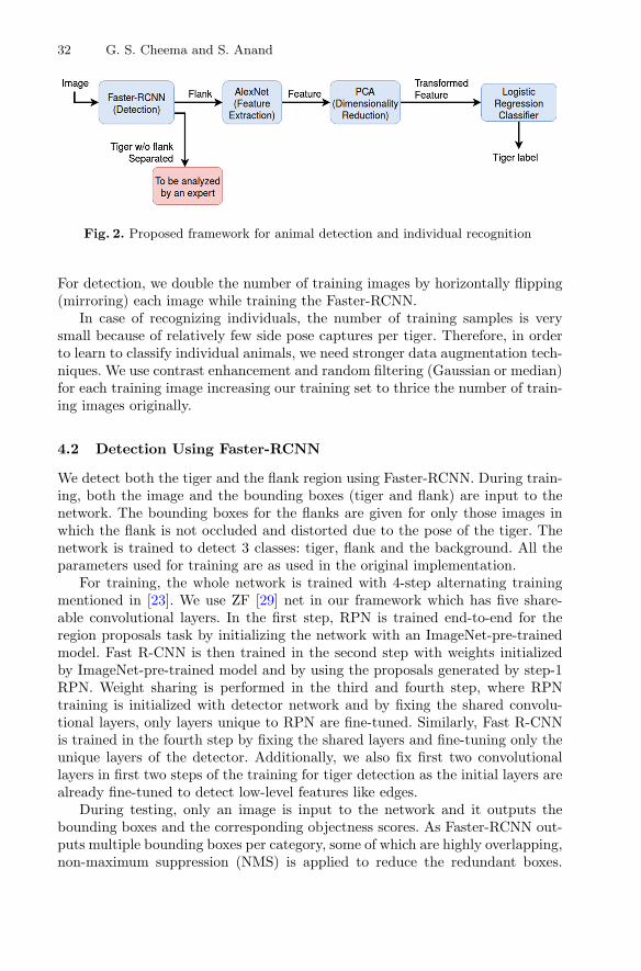
32 G. S. Cheema and S. Anand
Fig. 2. Proposed framework for animal detection and individual recognition
For detection, we double the number of training images by horizontally flipping(mirroring) each image while training the Faster-RCNN.
In case of recognizing individuals, the number of training samples is verysmall because of relatively few side pose captures per tiger. Therefore, in orderto learn to classify individual animals, we need stronger data augmentation tech-niques. We use contrast enhancement and random filtering (Gaussian or median)for each training image increasing our training set to thrice the number of train-ing images originally.
4.2 Detection Using Faster-RCNN
We detect both the tiger and the flank region using Faster-RCNN. During train-ing, both the image and the bounding boxes (tiger and flank) are input to thenetwork. The bounding boxes for the flanks are given for only those images inwhich the flank is not occluded and distorted due to the pose of the tiger. Thenetwork is trained to detect 3 classes: tiger, flank and the background. All theparameters used for training are as used in the original implementation.
For training, the whole network is trained with 4-step alternating trainingmentioned in [23]. We use ZF [29] net in our framework which has five share-able convolutional layers. In the first step, RPN is trained end-to-end for theregion proposals task by initializing the network with an ImageNet-pre-trainedmodel. Fast R-CNN is then trained in the second step with weights initializedby ImageNet-pre-trained model and by using the proposals generated by step-1RPN. Weight sharing is performed in the third and fourth step, where RPNtraining is initialized with detector network and by fixing the shared convolu-tional layers, only layers unique to RPN are fine-tuned. Similarly, Fast R-CNNis trained in the fourth step by fixing the shared layers and fine-tuning only theunique layers of the detector. Additionally, we also fix first two convolutionallayers in first two steps of the training for tiger detection as the initial layers arealready fine-tuned to detect low-level features like edges.
During testing, only an image is input to the network and it outputs thebounding boxes and the corresponding objectness scores. As Faster-RCNN out-puts multiple bounding boxes per category, some of which are highly overlapping,non-maximum suppression (NMS) is applied to reduce the redundant boxes.

Automatic Detection and Recognition of Individuals in Patterned Species 33
Because the convolution layers are shared, we can test the image in one go invery less time (0.3–0.6 s/image on a GPU).
4.3 Identification
For identification, we only use flank regions because they contain the discrim-inatory information to uniquely identify the patterned animals. The images inwhich the tiger is detected, but the flank is not, are separated to be analyzed bythe expert. A tool such as Extract-Compare [12] can be used for difficult caseswith extreme pose or occlusion.
We use ImageNet-pre-trained AlexNet [16] to extract features from the flankregion and train a logistic regression classifier to recognize the individuals. Whilethis deviates from the end-to-end framework, typical of deep networks, our choiceof this approach was to resolve the problem of very low training data for identify-ing individuals. We tried fine-tuning AlexNet with our data, however, the modeloverfitted the training set. For feature representation, we used different convo-lutional layers and fully connected layers to train our classifier and obtainedthe best results with the third convolutional layer (conv3). Since ImageNet is alarge-scale dataset, the pre-trained weights of AlexNet in the higher layers arenot optimized for a fine-grained task such as individual animal recognition. Onthe other hand, the middle layers (like conv3) capture interactions between edgesand are discriminative enough to give good results for our problem.
To minimize distortion introduced by resizing the detected flank region toa unit aspect ratio of AlexNet (227 × 227), we modify the size of input toAlexNet and hence the subsequent feature maps. Since the conv3 feature mapsare high dimensional, we apply a PCA (Principal Component Analysis) baseddimensionality reduction and use principal components that explain 99% of theenergy.
5 Experiments
All experiments are carried out with Python (and PyCaffe) running on i7-4720HQ 3.6 GHz processor and Nvidia GTX-950M GPU. For Faster-RCNN [23]training, we use a server with Nvidia GTX-980 GPU. We used the pythonimplementation of Faster-RCNN1 and labelImg2 annotation tool for annotat-ing the tiger and jaguar images. We also use python’s sklearn library for logisticregression classifier. Over three different datasets, we compare our results withHotSpotter [6], which showed superior performance as compared to Wild-ID [2]and StripeSpotter [17].
1 https://github.com/rbgirshick/py-faster-rcnn.2 https://github.com/tzutalin/labelImg.
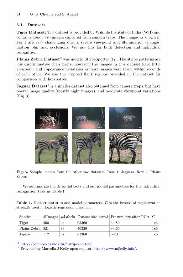
34 G. S. Cheema and S. Anand
5.1 Datasets
Tiger Dataset: The dataset is provided by Wildlife Institute of India (WII) andcontains about 770 images captured from camera traps. The images as shown inFig. 1 are very challenging due to severe viewpoint and illumination changes,motion blur and occlusions. We use this for both detection and individualrecognition.
Plains Zebra Dataset3 was used in StripeSpotter [17]. The stripe patterns areless discriminative than tigers, however, the images in this dataset have littleviewpoint and appearance variations as most images were taken within secondsof each other. We use the cropped flank regions provided in the dataset forcomparison with hotspotter.
Jaguar Dataset4 is a smaller dataset also obtained from camera traps, but havepoorer image quality (mostly night images), and moderate viewpoint variations(Fig. 3).
Fig. 3. Sample images from the other two datasets. Row 1: Jaguars. Row 2: PlainsZebra.
We summarize the three datasets and our model parameters for the individualrecognition task in Table 1.
Table 1. Dataset statistics and model parameters. C is the inverse of regularizationstrength used in logistic regression classifier.
Species #Images #Labels Feature size conv3 Feature size after PCA C
Tiger 260 44 63360 ∼180 1e6
Plains Zebra 821 83 40320 ∼460 1e6
Jaguar 112 37 63360 ∼70 1e5
3 http://compbio.cs.uic.edu/∼stripespotter/.4 Provided by Marcella J Kelly upon request: http://www.mjkelly.info/.
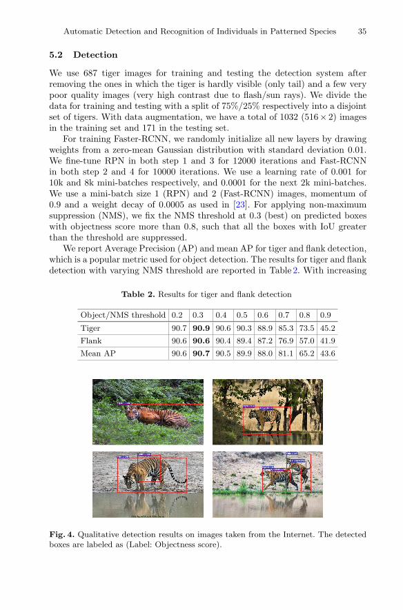
Automatic Detection and Recognition of Individuals in Patterned Species 35
5.2 Detection
We use 687 tiger images for training and testing the detection system afterremoving the ones in which the tiger is hardly visible (only tail) and a few verypoor quality images (very high contrast due to flash/sun rays). We divide thedata for training and testing with a split of 75%/25% respectively into a disjointset of tigers. With data augmentation, we have a total of 1032 (516× 2) imagesin the training set and 171 in the testing set.
For training Faster-RCNN, we randomly initialize all new layers by drawingweights from a zero-mean Gaussian distribution with standard deviation 0.01.We fine-tune RPN in both step 1 and 3 for 12000 iterations and Fast-RCNNin both step 2 and 4 for 10000 iterations. We use a learning rate of 0.001 for10k and 8k mini-batches respectively, and 0.0001 for the next 2k mini-batches.We use a mini-batch size 1 (RPN) and 2 (Fast-RCNN) images, momentum of0.9 and a weight decay of 0.0005 as used in [23]. For applying non-maximumsuppression (NMS), we fix the NMS threshold at 0.3 (best) on predicted boxeswith objectness score more than 0.8, such that all the boxes with IoU greaterthan the threshold are suppressed.
We report Average Precision (AP) and mean AP for tiger and flank detection,which is a popular metric used for object detection. The results for tiger and flankdetection with varying NMS threshold are reported in Table 2. With increasing
Table 2. Results for tiger and flank detection
Object/NMS threshold 0.2 0.3 0.4 0.5 0.6 0.7 0.8 0.9
Tiger 90.7 90.9 90.6 90.3 88.9 85.3 73.5 45.2
Flank 90.6 90.6 90.4 89.4 87.2 76.9 57.0 41.9
Mean AP 90.6 90.7 90.5 89.9 88.0 81.1 65.2 43.6
Fig. 4. Qualitative detection results on images taken from the Internet. The detectedboxes are labeled as (Label: Objectness score).

36 G. S. Cheema and S. Anand
NMS threshold, number of output bounding boxes also increase which leads topoor detection results. We also show some qualitative results on tiger imagestaken from the Internet, which are quite different in quality and backgroundwhen compared to the camera trap images as shown in Fig. 4.
5.3 Individual Recognition
We use conv3 features of AlexNet for training a logistic regression classifier toclassify individuals. For each dataset, we generate five random splits with 75%for training and 25% for testing. For our framework, flanks of tiger and jaguarare resized to 256 × 192 and for the zebra to 256× 128 which is equivalent toaverage size of flank images for the respective dataset. We learn a logistic regres-sion model with �1 regularization and perform grid search to find the parameterC. Specific data statistics and model parameters are reported in Table 1. Wecompare our results with HotSpotter and report the average rank 1 accuracyfor all the datasets in Table 3. In Fig. 5, we show the Cumulative Match Char-acteristic (CMC) curves from rank 1 to rank 5 for our method compared withHotspotter over all the datasets. The CMC curves indicate that the CNN basedarchitecture clearly works better than HotSpotter in case of stripe patterns, evenas we compare lower-rank accuracies. In the jaguar dataset, Hotspotter has amuch higher rank-1 accuracy, but we observe a rising trend of our deep learningbased approach as we compare lower-rank accuracies. We conjecture that thepre-trained AlexNet feature representation is not as discriminative for spots injaguars as in case of stripes in tigers or zebras.
Table 3. Average rank 1 accuracy comparison
Dataset Ours (227 × 227) Ours (resized) HotSpotter
Tiger 76.5 ± 2.2 80.5±2.1 75.3 ± 1.2
Jaguar 73.5 ± 1.8 78.6 ± 2.3 92.4±1.1
Zebra 91.1 ± 1.2 93.2±1.4 90.9 ± 0.8
(a) Zebra dataset (b) Tiger dataset (c) Jaguar dataset
Fig. 5. CMC curve comparison

Automatic Detection and Recognition of Individuals in Patterned Species 37
6 Conclusion
In this paper, we proposed a framework for automatic detection and individualrecognition in patterned animal species. We used the state-of-the-art CNN basedobject detector Faster-RCNN [23] and fine-tuned it for the purpose of detectingthe whole body and the flank of the tiger. We then used the detected flanks andextracted features from a pre-trained AlexNet [16] to train a logistic regressionclassifier for classifying individual tigers. We also performed individual recogni-tion task on zebras and jaguars. We get perfect results for tiger detection andperform better than Hotspotter [6] while comparing rank-1 accuracy for individ-ual recognition for tiger and zebra images. Even though AlexNet [16] featuresused for individual recognition are trained on Imagenet data, they seem to be asrobust as SIFT [18] features as shown by our quantitative results. We plan doa thorough comparison in future with larger datasets to obtain deeper insights.For jaguar images, Hotspotter works better at rank-1 accuracy, but the proposedmethod shows improving trends as we compare lower-rank accuracies.
Acknowledgments. The authors would like to thank WII for providing the tigerdata, Infosys Center for AI at IIIT-Delhi for computing resources and the anonymousreviewers for their invaluable comments.
References
1. Ahonen, T., Hadid, A., Pietikainen, M.: Face description with local binary patterns:application to face recognition. IEEE TPAMI 28(12), 2037–2041 (2006)
2. Bolger, D.T., Morrison, T.A., Vance, B., Lee, D., Farid, H.: A computer-assistedsystem for photographic mark-recapture analysis. Methods Ecol. Evol. 3(5), 813–822 (2012)
3. Burghardt, T., Calic, J.: Real-time face detection and tracking of animals. In:Neural Network Applications in Electrical Engineering, pp. 27–32. IEEE (2006)
4. Burghardt, T., Calic, J., Thomas, B.T.: Tracking animals in wildlife videos usingface detection. In: EWIMT (2004)
5. Cohen, I., et al.: Facial expression recognition from video sequences: temporal andstatic modeling. CVIU 91(1), 160–187 (2003)
6. Crall, J.P., et al.: Hotspotter - patterned species instance recognition. In: WACV,pp. 230–237. IEEE (2013)
7. Daugman, J.: How iris recognition works. IEEE Trans. Circuits Syst. Video Tech-nol. 14(1), 21–30 (2004)
8. Felzenszwalb, P.F., Girshick, R.B., McAllester, D., Ramanan, D.: Object detectionwith discriminatively trained part-based models. IEEE TPAMI 32(9), 1627–1645(2010)
9. Freytag, A., Rodner, E., Simon, M., Loos, A., Kuhl, H.S., Denzler, J.: Chimpanzeefaces in the wild: log-Euclidean CNNs for predicting identities and attributes ofprimates. In: Rosenhahn, B., Andres, B. (eds.) GCPR 2016. LNCS, vol. 9796, pp.51–63. Springer, Cham (2016). https://doi.org/10.1007/978-3-319-45886-1 5
10. Girshick, R.: Fast R-CNN. In: ICCV, pp. 1440–1448 (2015)11. He, K., Zhang, X., Ren, S., Sun, J.: Deep residual learning for image recognition.
CVPR, 770–778 (2016)

38 G. S. Cheema and S. Anand
12. Hiby, L., Lovell, P., Patil, N., Kumar, N.S., Gopalaswamy, A.M., Karanth, K.U.: Atiger cannot change its stripes: using a three-dimensional model to match imagesof living tigers and tiger skins. Biol. Lett. 5(3), 383–386 (2009)
13. Jain, A.K., Prabhakar, S., Hong, L., Pankanti, S.: Filterbank-based fingerprintmatching. IEEE Trans. Image Process. 9(5), 846–859 (2000)
14. Jiang, X., Yau, W.Y.: Fingerprint minutiae matching based on the local and globalstructures. In: ICPR, vol. 2, pp. 1038–1041. IEEE (2000)
15. Klingel, A.: Social organization and behavior of grevy’s zebra (Equus grevyi). Z.Tierpsychol. 36, 37–70 (1974)
16. Krizhevsky, A., Sutskever, I., Hinton, G.E.: ImageNet classification with deep con-volutional neural networks. In: NIPS, pp. 1097–1105 (2012)
17. Lahiri, M., Tantipathananandh, C., Warungu, R., Rubenstein, D.I., Berger-Wolf,T.Y.: Biometric animal databases from field photographs: identification of individ-ual zebra in the wild. In: International Conference on Multimedia Retrieval, p. 6.ACM (2011)
18. Lowe, D.G.: Distinctive image features from scale-invariant keypoints. Int. J. Com-put. Vision 60(2), 91–110 (2004)
19. Mizroch, S.A., Harkness, S.A.: A test of computer-assisted matching using theNorth Pacific humpback whale, Megaptera novaeangliae, tail flukes photographcollection. Mar. Fisheries Rev. 65(3), 25–37 (2003)
20. Norouzzadeh, M.S., Nguyen, A., Kosmala, M., Swanson, A., Packer, C., Clune, J.:Automatically identifying wild animals in camera trap images with deep learning.arXiv preprint arXiv:1703.05830 (2017)
21. Philbin, J., Chum, O., Isard, M., Sivic, J., Zisserman, A.: Object retrieval withlarge vocabularies and fast spatial matching. In: CVPR, pp. 1–8. IEEE (2007)
22. Prodger, P.: Darwin’s Camera: Art and Photography in the Theory of Evolution.Oxford University Press, New York (2009)
23. Ren, S., He, K., Girshick, R., Sun, J.: Faster R-CNN: towards real-time objectdetection with region proposal networks. In: NIPS, pp. 91–99 (2015)
24. Scott, D.K.: 17 identification of individual Bewick’s swans by bill patterns. Recog-nition Marking of Animals in Research, p. 160 (1978)
25. Simonyan, K., Zisserman, A.: Very deep convolutional networks for large-scaleimage recognition. arXiv preprint arXiv:1409.1556 (2014)
26. Swanson, A., Kosmala, M., Lintott, C., Simpson, R., Smith, A., Packer, C.: Snap-shot serengeti, high-frequency annotated camera trap images of 40 mammalianspecies in an African Savanna. Sci. Data 2, 150026 (2015)
27. Tisse, C.l., Martin, L., Torres, L., Robert, M., et al.: Person identification tech-nique using human iris recognition. In: Proceedings of Vision Interface, pp. 294–299(2002)
28. Turk, M.A., Pentland, A.P.: Face recognition using eigenfaces. In: CVPR, pp. 586–591. IEEE (1991)
29. Zeiler, M.D., Fergus, R.: Visualizing and understanding convolutional net-works. In: Fleet, D., Pajdla, T., Schiele, B., Tuytelaars, T. (eds.) ECCV 2014.LNCS, vol. 8689, pp. 818–833. Springer, Cham (2014). https://doi.org/10.1007/978-3-319-10590-1 53
30. Zhang, W., Sun, J., Tang, X.: From tiger to panda: animal head detection. IEEETrans. Image Process. 20(6), 1696–1708 (2011)
31. Zhu, X., Ramanan, D.: Face detection, pose estimation, and landmark localizationin the wild. In: CVPR, pp. 2879–2886. IEEE (2012)

Boosting Based Multiple Kernel Learningand Transfer Regression for Electricity Load
Forecasting
Di Wu1(B), Boyu Wang2, Doina Precup1, and Benoit Boulet1
1 McGill University, Montreal, QC H3A 0G4, [email protected], [email protected], [email protected]
2 Princeton University, Princeton, NJ 08544, [email protected]
Abstract. Accurate electricity load forecasting is of crucial importancefor power system operation and smart grid energy management. Differ-ent factors, such as weather conditions, lagged values, and day typesmay affect electricity load consumption. We propose to use multiple ker-nel learning (MKL) for electricity load forecasting, as it provides moreflexibilities than traditional kernel methods. Computation time is animportant issue for short-term load forecasting, especially for energyscheduling demand. However, conventional MKL methods usually leadto complicated optimization problems. Another practical aspect of thisapplication is that there may be very few data available to train a reli-able forecasting model for a new building, while at the same time wemay have prior knowledge learned from other buildings. In this paper,we propose a boosting based framework for MKL regression to deal withthe aforementioned issues for short-term load forecasting. In particular,we first adopt boosting to learn an ensemble of multiple kernel regres-sors, and then extend this framework to the context of transfer learning.Experimental results on residential data sets show the effectiveness ofthe proposed algorithms.
Keywords: Electricity load forecasting · BoostingMultiple kernel learning · Transfer learning
1 Introduction
Electricity load forecasting is very important for the economic operation andsecurity of a power system. The accuracy of electricity load forecasting directlyinfluences the control and planning of power system operation. It is estimatedthat a 1% increase of forecasting error would bring in a 10 million pounds increasein operating cost per year (in 1984) for the UK power system [4]. Experts believethat this effect could become even stronger, due to the emergence of highly uncer-tain energy sources, such as solar and wind energy generation. Depending on the
c© Springer International Publishing AG 2017Y. Altun et al. (Eds.): ECML PKDD 2017, Part III, LNAI 10536, pp. 39–51, 2017.https://doi.org/10.1007/978-3-319-71273-4_4

40 D. Wu et al.
lead time horizon, electricity load forecasting ranges from short-term forecast-ing (minutes or hours ahead) to long-term forecasting (years ahead) [13]. Withincreasingly competitive markets and demand response energy management [15],short-term load forecasting is becoming more and more important [25]. In thispaper, therefore, we will focus on tackling this problem.
Electricity load forecasting is a very difficult task since the load is influencedby many uncertain factors. Various methods have been proposed for electricityload forecasting including statistical methods, time series analysis, and machinelearning algorithms [21]. Some recent work uses multiple kernels to build predic-tion models for electricity load forecasting. For example, in [1], Gaussian kernelswith different parameters are applied to learn peak power consumption. In [8],different types of kernels are used for different features and a multi-task learn-ing algorithm is proposed and applied on low level load consumption data toimprove the aggregated load forecasting accuracy. However, all of the existingmethods rely on a fixed set of coefficients for the kernels (i.e., simply set to 1),implicitly assuming that all the kernels are equally important for forecasting,which is suboptimal in real world applications.
Multiple kernel learning (MKL) [2], which learns both the kernels and theircombination weights for different kernels, could be tailored to this problem.Through MKL, different kernels could have different weights according to theirinfluence on the outputs. However, learning with multiple kernels usually involvesa complicated convex optimization problem, which limits their application onlarge scale problems. Although some progresses have been made in improvingthe efficiency of the learning algorithms, most of them only focus on classifica-tion tasks [23,26]. On the other hand, electricity load forecasting is a regressionproblem and the computation time is an important issue.
Another practical issue for load forecasting is the lack of data to build areliable forecasting model. For example, consider the case of a set of newly builthouses (target domain) for which we want to predict the load consumption. Wemay not have enough data to build a prediction model for these new houses,while we have a large amount of data or knowledge from other houses (sourcedomain). The challenge here is to perform transfer learning [18], which relies onthe assumption is that there are some common structures or factors that can beshared across the domains. The objective of transfer learning for load forecastingis to improve the forecasting performance by discovering shared knowledge andleveraging it for electricity load prediction for target buildings.
In this paper, we address both challenges within a novel boosting-based MKLframework. In particular, we first propose the boosting based multiple kernelregression (BMKR) algorithm to improve the computational efficiency of MKL.Furthermore, we extend BMKR to the context of transfer learning, and pro-pose two variants of BMKR: kernel-level boosting based transfer multiple kernelregression (K-BTMKR) and model-level gradient boosting based transfer multiplekernel regression (M-BTMKR). Our contribution, from an algorithmic perspec-tive, is two-fold: We propose a boosting based learning framework (1) to learnregression models with multiple kernels efficiently, and (2) to leverage the MKL

Boosting Based Multiple Kernel Learning and Transfer Regression 41
models learned from other domains. On the application side, this work intro-duces the use of transfer learning for the load forecasting problem, which opensup potential future work avenues.
2 Background
2.1 Multiple Kernel Regression
Let S = {(xn, yn), n = 1, . . . , N} ∈ Rd × R be the data set with N samples,
K = {km : Rd ×Rd → R,m = 1, . . . , M} be M kernel functions. The objective of
MKL is to learn a prediction model, which is a linear combination of M kernels,by solving the following optimization problem [11]:
minη∈Δ
minF∈HK
12||F ||2K + C
N∑
n=1
�(F (xn), yn), (1)
where Δ = {η ∈ R+|∑Mm=1 ηm = 1} is a set of weights, HK is the
reproducing kernel Hilbert space (RKHS) induced by the kernel K(x, xn) =∑Mm=1 ηmkm(x, xn) and �(F (x), y) is a loss function. In this paper we use the
squared loss �(F (x), y) = 12 (F (x) − y)2 for the regression problem. The solution
of Eq. 1 is of the form1
F (x) =N∑
n=1
αnK(x, xn), (2)
where the coefficients {αn} and {ηm} are learned from samples.Compared with single kernel approaches, MKL algorithms can provide bet-
ter learning capability and alleviate the burden of designing specific kernels tohandle diverse multivariate data.
2.2 Gradient Boosting and ε-Boosting
Gradient boosting [10,16] is an ensemble learning framework which combinesmultiple hypotheses by performing gradient descent in function space. Morespecifically, the model learned by gradient boosting can be expressed as:
F (x) =T∑
t=1
ρtf t(x), (3)
where T is the number of total boosting iterations, and the t-th base learner f t
is selected such that the distance between f t and the negative gradient of theloss function at F = F t−1 is minimized:
f t = arg minf
N∑
n=1
(f(xn) − rt
n
)2, (4)
1 We ignore the bias term for simplicity of analysis, but in practice, the regressionfunction can accomodate both the kernel functions and the bias term.

42 D. Wu et al.
where rtn = −
[∂�(F (xn),yn)
∂F
]
F=F t−1, and ρt is the step size which can either
be fixed or chosen by line search. Plugging in the squared loss we have rtn =
yn − F t−1(xn). In other words, gradient boosting with squared loss essentiallyfits the residual at each iteration.
Let F = {f1, . . . , fJ} be a set of candidate functions, where J = |F| is thesize of the function space, and f : Rd → R
J , f(x) = [f1(x), . . . , fJ (x)]� be themapping defined by F . Gradient boosting with squared loss usually proceedsin a greedy way: the step size is simply set ρt = 1 for all iterations. On theother hand, if the step size ρt is set to some small constant ε > 0, it can beshown that under the monotonicity condition, this example of gradient boostingalgorithm, referred to as ε-boosting in [20], essentially solves an �1-regularizedlearning problem [12]:
min||β||1≤μ
N∑
n=1
1N
�(β�f(xn), yn
), (5)
where β ∈ RJ is the coefficient vector, and μ is the regularization parameter, such
that εT ≤ μ. In other words, ε-boosting implicitly controls the regularization viathe number of iterations T rather than μ.
2.3 Transfer Learning from Multiple Sources
Let ST = {(xn, yn), n = 1, . . . , N} be the data set from the target domain,and {S1, . . . ,SS} be the data sets from S source domains, where Ss ={(xs
n, ysn), n = 1, . . . , Ns} are the samples of the s-th source. Let {F1, . . . , FS}
be the prediction models learned from S source domains. In this work, the s-thmodel Fs is trained by some MKL algorithm (e.g., BMKR), and is of the form:
Fs =M∑
m=1
ηsmhs
m(x) =M∑
m=1
ηsm
Ns∑
n=1
αsnkm(x, xs
n). (6)
The objective of transfer learning is to build a model F that has a goodgeneralization ability in the target domain using the data set ST (which is typi-cally small) and knowledge learned from sources {S1, . . . ,SS}. In this work, weassume that such knowledge has been embedded into {F1, . . . , FS}, and thereforethe problem becomes to explore the model structures that can be transferred tothe target domain from various source domains. This type of learning approachis also referred to as parameter transfer [18].
3 Methods
3.1 Boosting Based Multiple Kernel Learning Regression
The idea of BMKR is to learn an ensemble model with multiple kernel regressorsusing the gradient boosting framework. The starting point of our method is sim-ilar to multiple kernel boosting (MKBoost) [23], which adapts AdaBoost [9] for

Boosting Based Multiple Kernel Learning and Transfer Regression 43
Algorithm 1. BMKR: Boosting based Multiple Kernel RegressionInput: Data set S, kernel functions K, number of iterations T
1: Initialize residual: r1n = yi, ∀n ∈ {1, . . . , N}, and F = 02: for t = 1, ..., T do3: for m = 1, ..., M do4: Sample N ′ data points from S5: Train a kernel regression model f t
m with km by fitting the residuals of theselected N ′ samples
6: Compute the loss: etm = 1
2
∑Nn=1
(f t
m(xn) − rtn
)2
7: end for8: Select the regression model with the smallest fitting error: f t = arg minft
met
m
9: Add f t to the ensemble: F ← F + εf t
10: Update residuals: rt+1n = yn − F (xn), ∀n ∈ {1, 2, ...N}
11: end for
Output: the final multiple kernel function F (x)
multiple kernel classification. We extend this idea to a more general frameworkof gradient boosting [10,16], which allows different loss functions for differenttypes of learning problems. In this paper, we focus on the regression problemand use the squared loss.
At the t-th boosting iteration, for each kernel km,m = 1, . . . , M , we first traina kernel regression model such as support vector regression (SVR) by fitting thecurrent residuals, and obtain a solution of the form:
f tm(x) =
N∑
n=1
αt,nkm(x, xn). (7)
Then we choose from M candidates, the regression model with the smallestfitting error
f t = arg minftm,m∈{1,...,M}
etm, (8)
where etm = 1
2
∑Nn=1 (f t
m(xn) − rtn)2, and add it to the ensemble F . The final
hypothesis of BMKR is expressed as in Eq. 3.The pseudo-code of BMKR is shown in Algorithm 1. For gradient boosting
with squared loss, the step size ρt is not strictly necessary [3], and we can eithersimply set it to 1, or a fixed small value ε as suggested by ε-boosting. Note thatat each boosting iteration, instead of fitting all N samples, we can select only N ′
samples for training a SVR model, as suggested in [23], which can substantiallyreduce the computational complexity of each iteration as N ′ � N .
3.2 Boosting Based Transfer Regression
As explained in Sect. 1, as we typically have very few data in the target domain,and therefore the model can easily overfit, especially if we train a complicated

44 D. Wu et al.
MKL model, even with the boosting approach. To deal with this issue, we canimplicitly regularize the candidate functions at each boosting iteration by con-straining the learning process within the function space spanned by the kernelfunctions trained on the source domains, rather than training the model in thefunction space spanned by arbitrary kernels. On the other hand, however, theunderlying assumption of this approach is that at least one source domain isclosely related to the target domain and therefore the kernel functions learnedfrom the source domains can be reused. If this assumption does not hold, negativetransfer could hurt the prediction performance. To avoid this situation, we alsokeep a MKL model which is trained only on the target domain. Consequently,the challenge becomes how to balance the knowledge embedded in the modellearned from the source domains and the data fitting in the target domain.
To address this issue in a principled manner, we follow the idea of ε-boosting [6,20] and propose the BTMKR algorithm, which is aimed towardstransfer learning. There are two levels of transferring the knowledge of mod-els: kernel-level transfer and model-level transfer, denoted by K-BTMKR andM-BTMKR respectively. At each iteration, K-BTMKR selects a single kernelfunction from S × M candidate kernels, while M-BTMKR selects a multiplekernel model from S domains. Therefore, K-BTMKR has higher “resolution”and more flexibility, at the price of higher risk of overfitting, as the dimensionof its search space is M higher than that of M-BTMKR.
Kernel-Level Transfer (K-BTMKR). Let H = {h11, . . . , h
1M , . . . , hS
1 , . . . ,hS
M} be the set of MS candidate kernel functions learned from S source domains,and F = {f1, . . . , fJ} be the set of J candidate kernel functions from the targetdomain. Note that as the kernel functions from the source domains are fixed,the size of H is finite, while the size of the function space of the target domainis infinite, since the weights learned by SVR can be arbitrary (i.e., Eq. 7). Forsimplicity of analysis, we assume J is also finite. Given the mapping h : Rd →R
MS , h(x) = [h11(x), . . . , hS
M ]� defined by H and the mapping f defined by F ,we formulate the transfer learning problem as:
minβS ,βT
L (βS , βT ) s.t. ||βS ||1 + λ||βT ||1 ≤ μ, (9)
where L(βS , βT ) �∑N
n=1 �(β�S h(xn) + β�
T f(xn), yn), βS � [β11 , . . . , β
SM ]� ∈
RMS , βT � [β1, . . . , βJ ]� ∈ R
J are the coefficient vectors for the source domainsand the target domain respectively, and λ is a parameter that controls how muchwe penalize βT against βS . Intuitively, if the data from target domain is limited,we should set λ ≥ 1 to favor the model learned from the source domains, inorder to avoid overfitting.
Following the idea of ε-boosting [12,20], Eq. 9 can be solved by slowly increas-ing the value of μ by ε, from 0 to a desired value. More specifically, let g(x) =[h(x)�, f(x)�]�, and β =
[Δβ�
S ,Δβ�T
]�. At the t-th boosting iteration, the

Boosting Based Multiple Kernel Learning and Transfer Regression 45
coefficient vector β is updated to β + Δβ by solving the following optimizationproblem:
minΔβ
L (β + Δβ) s.t. ||ΔβS ||1 + λ||ΔβT ||1 ≤ ε (10)
As ε is very small, the objective function of Eq. 10 can be expanded by first-orderTaylor expansion, which gives
L (β + Δβ) ≈ L (β) + ∇L (β)�Δβ, (11)
where
∂L∂βj
=N∑
n=1
−rtngj(xn), ∀j ∈ {1, . . . , MS + J}. (12)
By changing the coefficients βT ← λβT , it can be shown that minimizing Eq. 10can be (approximately) solved by
Δβj =
{ε, if j = arg maxj
∑Nn=1 rt
ngj(xn)
λj
0, otherwise, (13)
where λj = 1,∀j ∈ {1, . . . , MS}, and λj = λ, otherwise. In practice, as thesize of function space of target domain is infinite, the candidate functions areactually computed by fitting the current residuals, as shown in Algorithm 2.
Model-Level Transfer (M-BTMKR). The derivation of M-BTMKR is sim-ilar to that of K-BTMKR, and therefore is omitted here.
3.3 Computational Complexity
The computational complexity of BMKR, as analyzed in [23], is O(TMξ(N)),where ξ(N) is the computational complexity of training a single SVR with Nsamples. Standard learning approaches formulate SVR as a quadratic program-ming (QP) problem and therefore ξ(N) is O(N3). Lower complexity (e.g., aboutO(N2)) can be achieved by using other solvers (e.g., LIBSVM [5]). More impor-tant, BMKR can adopt stochastic learning approach, as suggested in [23], whichonly selects N ′ samples for training a SVR at each boosting iteration. This app-roach yields a complexity of O(TM(N + ξ(N ′))), which makes the algorithmtractable for large-scale problems by choosing N ′ � N . The computationalcomplexity of the BTMKR algorithms is O(TM(SN + ξ(N))). Note that in thecontext of transfer learning, we use all the samples from the target domain, asthe size of data set is usually small.
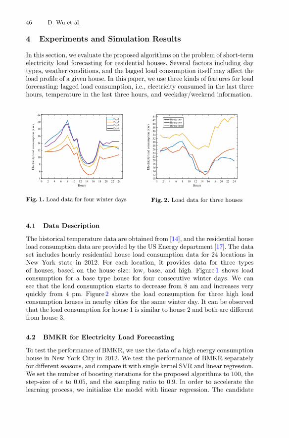
46 D. Wu et al.
4 Experiments and Simulation Results
In this section, we evaluate the proposed algorithms on the problem of short-termelectricity load forecasting for residential houses. Several factors including daytypes, weather conditions, and the lagged load consumption itself may affect theload profile of a given house. In this paper, we use three kinds of features for loadforecasting: lagged load consumption, i.e., electricity consumed in the last threehours, temperature in the last three hours, and weekday/weekend information.
0 2 4 6 8 10 12 14 16 18 20 22 24Hours
4
6
8
10
12
14
16
18
20
22
Elec
trici
ty lo
ad c
onsu
mpt
ion
(kW
)
Day1Day2Day3Day4
Fig. 1. Load data for four winter days
0 2 4 6 8 10 12 14 16 18 20 22 24Hours
101214161820222426283032343638404244
Elec
trici
ty lo
ad c
onsu
mpt
ion
(kW
)
House oneHouse twoHouse three
Fig. 2. Load data for three houses
4.1 Data Description
The historical temperature data are obtained from [14], and the residential houseload consumption data are provided by the US Energy department [17]. The dataset includes hourly residential house load consumption data for 24 locations inNew York state in 2012. For each location, it provides data for three typesof houses, based on the house size: low, base, and high. Figure 1 shows loadconsumption for a base type house for four consecutive winter days. We cansee that the load consumption starts to decrease from 8 am and increases veryquickly from 4 pm. Figure 2 shows the load consumption for three high loadconsumption houses in nearby cities for the same winter day. It can be observedthat the load consumption for house 1 is similar to house 2 and both are differentfrom house 3.
4.2 BMKR for Electricity Load Forecasting
To test the performance of BMKR, we use the data of a high energy consumptionhouse in New York City in 2012. We test the performance of BMKR separatelyfor different seasons, and compare it with single kernel SVR and linear regression.We set the number of boosting iterations for the proposed algorithms to 100, thestep-size of ε to 0.05, and the sampling ratio to 0.9. In order to accelerate thelearning process, we initialize the model with linear regression. The candidate

Boosting Based Multiple Kernel Learning and Transfer Regression 47
kernels for BMKR are: Gaussian kernels with 10 different widths (2−4, 2−3, ..., 25)and a linear kernel. We repeat the simulation for 10 times, and each time werandomly choose 50% of the data in the season as training data and 50% of thedata as testing data.
Table 1 shows the mean and standard deviation (std dev) of the Mean Aver-age Percentage Error (MAPE) measurement for BMKR and the other two base-lines. We can see that BMKR achieves the best forecasting performance forall seasons, obtaining 3.3% and 3.8% average MAPE improvements over linearregression and single kernel SVR respectively.
Table 1. MAPE (%) performance (mean ± std dev) for high load consumption houses
Method Spring Summer Fall Winter Average
Linear 10.42 ± 0.10 7.78 ± 0.13 9.21 ± 0.22 5.81 ± 0.13 8.30 ± 0.15
SVR 10.95 ± 0.21 7.73 ± 0.11 8.82 ± 0.21 5.88 ± 0.12 8.34 ± 0.16
BMKR 10.31± 0.17 7.64± 0.02 8.42 ± 0.11 5.73± 0.07 8.02± 0.10
4.3 Transfer Regression for Electricity Load Forecasting
We evaluate the proposed transfer regression algorithms: M-BTMKR andK-BTMKR on high load consumption houses. We randomly pick 6 high loadconsumption houses as target house and use the remaining 18 high consumptionhouses as source houses. We repeat the simulation 10 times for each house, andeach time we randomly choose 36 samples as the training data, and 100 samplesas the testing data for the target house. For source houses, we randomly chose600 data samples as the training data in each simulation. For K-BTMKR andM-BTMKR, λ is chosen by cross validation to balance the model leaned fromsource house data and the model learned from target house data.
Performance of M-BTMKR and K-BTMKR are compared with linear regres-sion, single kernel SVR and BMKR. The candidate kernels and boosting set-ting are the same as in Sect. 4.2. For the baselines, the forecasting models aretrained only with data from target houses, and the results are shown in Table 22,from which it can be observed that the proposed transfer algorithms signifi-cantly improve the forecasting performance. For each individual location, thebest results are achieved by either K-BTMKR or M-BTMKR, and M-BTMKRshows the best performance on average. The forecasting accuracies of M-BTMKRand K-BTMKR are very close to each other and both are much better than thebaseline algorithms without transfer. In other words, with the proposed transferalgorithms, the knowledge learned from the source houses is properly transferredto the target house.
2 Due to the space limitation, we only report the results for high load consumptionhouses. The results for low and base load consumption houses are similar to the highload consumption houses.

48 D. Wu et al.
Table 2. Transfer learning MAPE (%) performance for high load consumption houses
Method Location 1 Location 2 Location 3 Location 4 Location 5 Location 6 Average
Linear 8.02± 0.05 9.11± 0.70 17.39± 1.62 6.05± 0.02 11.43± 0.15 9.42± 0.65 10.24± 0.53
SVR 11.53± 0.34 6.82± 0.39 25.90± 0.72 8.24± 0.08 26.31± 1.97 14.00± 0.65 15.47± 0.69
BMKR 8.06± 0.03 6.64± 0.54 17.85± 1.31 5.29± 0.01 12.82± 0.21 9.05± 0.57 9.95± 0.45
M-BTMKR 5.35± 0.01 5.99± 0.02 5.63± 0.19 5.01± 0.01 9.13± 0.01 5.69± 0.01 6.13± 0.04
K-BTMKR 5.38± 0.02 5.46± 0.30 6.97± 0.26 5.55± 0.09 8.96± 0.14 7.31± 0.21 6.60± 0.17
4.4 Negative Transfer Analysis
Sometimes the consumption pattern for source houses and target houses can bequite different. We would prefer that the transfer algorithms prevent potentialnegative transfer for such scenarios. Here we present a case study to show theimportance of balancing the knowledge learned from source domains and datafitting in the target domain. We use the same high load target houses as describedin Sect. 4.3, but for the source houses, we randomly chose eighteen houses fromthe low type houses. We repeat the simulation for 10 times and the results areshown in Table 3.
The proposed algorithms are compared with linear regression, single kernelSVR, BMKR, M-BTMKRwoT , and K-BTMKRwoT , where M-BTMKRwoT andK-BTMKRwoT denote the BTMKR algorithms that we do not keep a MKLmodel trained on the target domain when we learn BTMKR models (i.e., wedo not train f∗ in Algorithm 2). Simulation results show that, if we do notkeep a MKL model trained on the target domain, we would encounter severenegative transfer problem, and the forecasting accuracy would be even muchworse than the models learned without transfer. Meanwhile, we can see thatthe proposed M-BTMKR and K-BTMKR could successfully avoid such negativetransfer. In this case, M-BTMKR and K-BTMKR still show better performancethan other algorithms, though the forecasting accuracy of K-BTMKR is veryclose to BMKR. M-BTMKR achieves the best average forecasting performanceand provides 14.37% average forecasting accuracy improvements over BMKR.In summary, the BTMKR algorithms can avoid the negative transfer when thedata distributions of source domain and target domain are quite different.
Table 3. Transfer learning MAPE (%) performance for high load consumption targethouses with low load consumption source houses

Boosting Based Multiple Kernel Learning and Transfer Regression 49
Algorithm 2. BTMKR: Boosting based Transfer Multiple Kernel RegressionInput: Data set ST from the target domain, number of iterations T , regularizationparameter λ, multiple kernel functions {F1, . . . , FS} learned from S source domains,where each Fs is given by Eq. 6.
1: Initialize residual: r1n = yn, ∀n ∈ {1, . . . , N}, and F = 02: for t = 1, ..., T do3: Compute the regression model f∗ and h∗ (line 8 – 21)
4: Select the base learner: f t =
{f∗, if
∑Nn=1 rt
nf∗(xn)
λ>
∑Nn=1 rt
nh∗(xn)
h∗, otherwise.
5: Add f t to the ensemble: F ← F + εf t
6: Update residuals: rt+1n = yn − F (xn), ∀n ∈ {1, 2, ...N}
7: end forOutput: the final multiple kernel function F (x)
K-BTMKR8: for s = 1, ..., S do9: for m = 1, ..., M do
10: Fit the current residuals: γts,m =
∑Nn=1 rt
nhsm(xn)
∑Nn=1 hs
m(xn)2
11: Compute the loss of hsm: et
s,m = 12
∑Nn=1
(γt
s,mhsm(xn) − rt
n
)2
12: end for13: end for14: Fit the residuals by training a kernel regressor:
f∗ = arg minf∈F 12
∑Nn=1
(f(xn) − rt
n
)
15: Return the regression models: f∗ and h∗ = arg min{hsm} et
s,m
M-BTMKR16: for s = 1, ..., S do
17: Fit the current residuals: γts =
∑Nn=1 rt
nFs(xn)∑N
n=1 Fs(xn)2
18: Compute the loss of Fs: ets = 1
2
∑Nn=1
(γt
sFs(xn) − rtn
)2
19: end for20: Fit the residuals by training a kernel regressor:
f∗ = arg minf∈F 12
∑Nn=1
(f(xn) − rt
n
)
21: Return the regression models: f∗ and h∗ = arg min{Fs} ets
5 Related Work
Various techniques have been proposed to efficiently learn MKL models [11],and our BMKR algorithm is originally inspired by [23], which applies the ideaof AdaBoost to train a multiple kernel based classifier. BMKR is a more generalframework which can adopt different loss functions for different learning tasks.Furthermore, the boosting approach provides a natural approach to solve smallsample size problems by leveraging transfer learning techniques. The originalwork on boosting based transfer learning proposed in [7] introduces a sample-reweighting mechanism based on AdaBoost for classification problem. Later, thisapproach is generalized to the cases of regression [19], and transferring knowledge

50 D. Wu et al.
from multiple sources [24]. In [6], a gradient boosting based algorithm is proposedfor multitask learning, where the assumption is that the model parameters ofall the tasks share a common factor. In [22], the transfer boosting and multitaskboosting algorithms are generalized to the context of online learning. While bothmultiple kernel learning and transfer learning have been studied extensively,the effort in simultaneously dealing with these two issues is very limited. OurBTMKR algorithm distinguishes itself from these methods because it deals withthese two learning problems in a unified and principled approach. To our bestknowledge, this is the first attempt to transfer MKL for regression problem.
6 Conclusion
In this paper, we first propose BMKR, a gradient boosting based multiple ker-nel learning framework for regression, which is suitable for short-term electricityload forecasting problems. Different from the traditional methods for MKL, theproposed BMKR algorithm learns the combination weights for each kernel usinga boosting-style algorithm. Simulation results on residential data show that theshort-term electricity load forecasting could be improved with BMKR. We fur-ther extend the proposed boosting framework to the context of transfer learningand propose two boosting based transfer multiple kernel regression algorithms:K-BTMKR and M-BTMKR. Empirical results suggest that both algorithmscan efficiently transfer the knowledge learned from source houses to the tar-get houses and significantly improve the forecasting performance when the tar-get houses and source houses have similar electricity load consumption pattern.We also investigate the effects of negative transfer and show that the proposedalgorithms could prevent potential negative transfer when the source houses arequite different from the target houses.
References
1. Atsawathawichok, P., Teekaput, P., Ploysuwan, T.: Long term peak load forecastingin Thailand using multiple kernel Gaussian process. In: ECTI-CON, pp. 1–4 (2014)
2. Bach, F.R., Lanckriet, G.R., Jordan, M.I.: Multiple kernel learning, conic duality,and the SMO algorithm. In: ICML, pp. 6–13 (2004)
3. Buhlmann, P., Hothorn, T.: Boosting algorithms: regularization, prediction andmodel fitting. Stat. Sci. 22, 477–505 (2007)
4. Bunn, D., Farmer, E.D.: Comparative Models for Electrical Load Forecasting. JohnWiley and Sons Inc., New York (1985)
5. Chang, C.C., Lin, C.J.: LIBSVM: a library for support vector machines. ACMTrans. Intell. Syst. Technol. 2(3), 27 (2011)
6. Chapelle, O., Shivaswamy, P., Vadrevu, S., Weinberger, K., Zhang, Y., Tseng, B.:Boosted multi-task learning. Mach. Learn. 85(1–2), 149–173 (2011)
7. Dai, W., Yang, Q., Xue, G.R., Yu, Y.: Boosting for transfer learning. In: ICML,pp. 193–200 (2007)
8. Fiot, J.B., Dinuzzo, F.: Electricity demand forecasting by multi-task learning.IEEE Trans. Smart Grid PP(99), 1 (2016)
Boosting Based Multiple Kernel Learning and Transfer Regression 51
9. Freund, Y., Schapire, R.E.: Experiments with a new boosting algorithm. In: ICML,pp. 148–156 (1996)
10. Friedman, J.H.: Greedy function approximation: a gradient boosting machine. Ann.Stat. 29, 1189–1232 (2001)
11. Gonen, M., Alpaydın, E.: Multiple kernel learning algorithms. J. Mach. Learn. Res.12, 2211–2268 (2011)
12. Hastie, T., Tibshirani, R., Friedman, J.: The Elements of Statistical Learning: DataMining, Inference, and Prediction, 2nd edn. Springer, New York (2009). https://doi.org/10.1007/978-0-387-84858-7
13. Hippert, H.S., Pedreira, C.E., Souza, R.C.: Neural networks for short-term loadforecasting: a review and evaluation. IEEE Trans. Power Syst. 16(1), 44–55 (2001)
14. IEM. https://mesonet.agron.iastate.edu/request/download.phtml15. Kamyab, F., Amini, M., Sheykhha, S., Hasanpour, M., Jalali, M.M.: Demand
response program in smart grid using supply function bidding mechanism. IEEETrans. Smart Grid 7(3), 1277–1284 (2016)
16. Mason, L., Baxter, J., Bartlett, P., Frean, M.: Boosting algorithms as gradientdescent in function space. In: NIPS, pp. 512–518 (2000)
17. OPENEI. http://en.openei.org/doe-opendata/dataset18. Pan, S.J., Yang, Q.: A survey on transfer learning. IEEE Trans. Knowl. Data Eng.
22(10), 1345–1359 (2010)19. Pardoe, D., Stone, P.: Boosting for regression transfer. In: ICML, pp. 863–870
(2010)20. Rosset, S., Zhu, J., Hastie, T.: Boosting as a regularized path to a maximum margin
classifier. J. Mach. Learn. Res. 5, 941–973 (2004)21. Soliman, S.A.H., Al-Kandari, A.M.: Electrical Load Forecasting: Modeling and
Model Construction. Elsevier, New York (2010)22. Wang, B., Pineau, J.: Online boosting algorithms for anytime transfer and multi-
task learning. In: AAAI, pp. 3038–3044 (2015)23. Xia, H., Hoi, S.C.: MKBoost: a framework of multiple kernel boosting. IEEE Trans.
Knowl. Data Eng. 25(7), 1574–1586 (2013)24. Yao, Y., Doretto, G.: Boosting for transfer learning with multiple sources. In:
CVPR, pp. 1855–1862 (2010)25. Zhang, R., Dong, Z.Y., Xu, Y., Meng, K., Wong, K.P.: Short-term load forecasting
of Australian National Electricity Market by an ensemble model of extreme learningmachine. IET Gener. Transm. Distrib. 7(4), 391–397 (2013)
26. Zhuang, J., Tsang, I.W., Hoi, S.C.: Two-layer multiple kernel learning. In: AIS-TATS, pp. 909–917 (2011)

CREST - Risk Prediction for ClostridiumDifficile Infection Using Multimodal
Data Mining
Cansu Sen1(B), Thomas Hartvigsen1, Elke Rundensteiner1,and Kajal Claypool2
1 Worcester Polytechnic Institute, Worcester, MA, USA{csen,twhartvigsen,rundenst}@wpi.edu
2 Harvard Medical School, Boston, MA, USAkajal [email protected]
Abstract. Clostridium difficile infection (CDI) is a common hospitalacquired infection with a $1B annual price tag that resulted in ∼30,000deaths in 2011. Studies have shown that early detection of CDI signif-icantly improves the prognosis for the individual patient and reducesthe overall mortality rates and associated medical costs. In this paper,we present CREST: CDI Risk Estimation, a data-driven framework forearly and continuous detection of CDI in hospitalized patients. CRESTuses a three-pronged approach for high accuracy risk prediction. First,CREST builds a rich set of highly predictive features from ElectronicHealth Records. These features include clinical and non-clinical pheno-types, key biomarkers from the patient’s laboratory tests, synopsis fea-tures processed from time series vital signs, and medical history minedfrom clinical notes. Given the inherent multimodality of clinical data,CREST bins these features into three sets: time-invariant, time-variant,and temporal synopsis features. CREST then learns classifiers for eachset of features, evaluating their relative effectiveness. Lastly, CRESTemploys a second-order meta learning process to ensemble these classi-fiers for optimized estimation of the risk scores. We evaluate the CRESTframework using publicly available critical care data collected for over12 years from Beth Israel Deaconess Medical Center, Boston. Our resultsdemonstrate that CREST predicts the probability of a patient acquir-ing CDI with an AUC of 0.76 five days prior to diagnosis. This valueincreases to 0.80 and even 0.82 for prediction two days and one day priorto diagnosis, respectively.
Keywords: Clostridium difficile · Risk stratificationMultimodal data mining · Multivariate time series classificationElectronic Health Records
c© Springer International Publishing AG 2017Y. Altun et al. (Eds.): ECML PKDD 2017, Part III, LNAI 10536, pp. 52–63, 2017.https://doi.org/10.1007/978-3-319-71273-4_5

CREST - Risk Prediction for Clostridium Difficile Infection 53
1 Introduction
Motivation. Clostridium difficile infection (CDI) is a common hospital acquiredinfection resulting in gastrointestinal illness with substantial impact on morbid-ity and mortality. In 2011, nearly half a million CDI infections were identified inthe US resulting in 29,000 patient deaths [1,11]. Despite well-known risk factorsand the availability of mature clinical practice guidelines [4], the infection andmortality rates of CDI continue to rise with an estimated $1 billion annual pricetag [7]. Early detection of CDI has been shown to be significantly correlatedwith a successful resolution of the infection within a few days, and is projectedto save $3.8 billion in medical costs over a period of 5 years [2]. In current prac-tice, a diagnostic test is usually ordered as a confirmation of a highly-suspectcase, only after appearance of symptoms1. This points to a tremendous oppor-tunity for employing machine learning techniques to develop intelligent systemsfor early detection of CDI to eradicate this medical crisis.
State-of-the-Art. Our literature review shows that there have been some ini-tial efforts to apply machine learning techniques to develop risk score estima-tion models for CDI. These efforts largely exploit two approaches. The first, amoment-in-time approach, uses only the data from one single moment in patient’sstay. This moment can be the admission time [14] or the most recent snapshotdata at the time of risk estimation [6]. The second, an independent-days app-roach, uses the complete hospital stay, but treats the days of a patient’s stayas independent from each other [16,17]. The complete physiological state of thepatient, changes in the physiological state, and clinical notes containing pastmedical information have been left out of the risk prediction process.
Challenges. To fill this gap, the following challenges must be addressed:
Varying Lengths of Patient Stays. Stay-lengths vary between patients, com-plicating the application of learning algorithms. Thus, we must design a fixed-length representation of time series patient-stay data. This requires temporalsummarization of data such that the most relevant information for the classifi-cation task is preserved.
Incorporating Clinical Notes. Clinical notes from a patient’s EHR con-tain vital information (e.g., co-morbidities and prior medications). These areoften taken in short-hand and largely abbreviated. Mining and analysis ofclinical notes is an open research problem, but some application of currenttechniques is necessary to transform them into a format usable for machinelearning algorithms.
Combining Multimodal Data. EHR data is typically multimodal, includingtext, static data and time series data, that require transformation and normal-ization prior to use in machine learning. The choices made when transforming
1 The authors would like to thank Elizabeth Claypool, RN, Coordinator of PatientSafety at U. Colorado Health for the valuable information she provided.
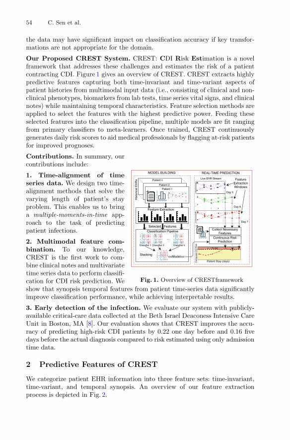
54 C. Sen et al.
the data may have significant impact on classification accuracy if key transfor-mations are not appropriate for the domain.
Our Proposed CREST System. CREST: CDI Risk Estimation is a novelframework that addresses these challenges and estimates the risk of a patientcontracting CDI. Figure 1 gives an overview of CREST. CREST extracts highlypredictive features capturing both time-invariant and time-variant aspects ofpatient histories from multimodal input data (i.e., consisting of clinical and non-clinical phenotypes, biomarkers from lab tests, time series vital signs, and clinicalnotes) while maintaining temporal characteristics. Feature selection methods areapplied to select the features with the highest predictive power. Feeding theseselected features into the classification pipeline, multiple models are fit rangingfrom primary classifiers to meta-learners. Once trained, CREST continuouslygenerates daily risk scores to aid medical professionals by flagging at-risk patientsfor improved prognoses.
Fig. 1. Overview of CRESTframework
Contributions. In summary, ourcontributions include:
1. Time-alignment of timeseries data. We design two time-alignment methods that solve thevarying length of patient’s stayproblem. This enables us to bringa multiple-moments-in-time app-roach to the task of predictingpatient infections.
2. Multimodal feature com-bination. To our knowledge,CREST is the first work to com-bine clinical notes and multivariatetime series data to perform classifi-cation for CDI risk prediction. Weshow that synopsis temporal features from patient time-series data significantlyimprove classification performance, while achieving interpretable results.
3. Early detection of the infection. We evaluate our system with publicly-available critical-care data collected at the Beth Israel Deaconess Intensive CareUnit in Boston, MA [8]. Our evaluation shows that CREST improves the accu-racy of predicting high-risk CDI patients by 0.22 one day before and 0.16 fivedays before the actual diagnosis compared to risk estimated using only admissiontime data.
2 Predictive Features of CREST
We categorize patient EHR information into three feature sets: time-invariant,time-variant, and temporal synopsis. An overview of our feature extractionprocess is depicted in Fig. 2.
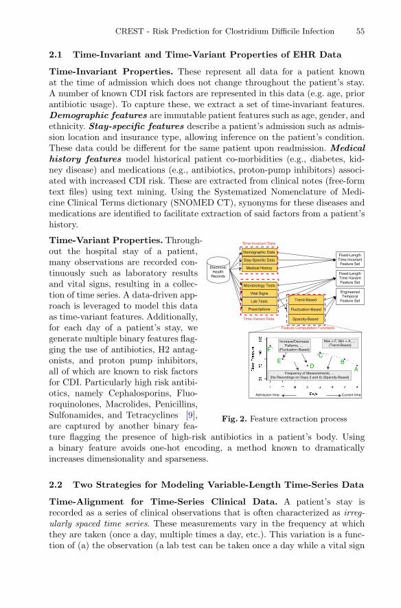
CREST - Risk Prediction for Clostridium Difficile Infection 55
2.1 Time-Invariant and Time-Variant Properties of EHR Data
Time-Invariant Properties. These represent all data for a patient knownat the time of admission which does not change throughout the patient’s stay.A number of known CDI risk factors are represented in this data (e.g. age, priorantibiotic usage). To capture these, we extract a set of time-invariant features.Demographic features are immutable patient features such as age, gender, andethnicity. Stay-specific features describe a patient’s admission such as admis-sion location and insurance type, allowing inference on the patient’s condition.These data could be different for the same patient upon readmission. Medicalhistory features model historical patient co-morbidities (e.g., diabetes, kid-ney disease) and medications (e.g., antibiotics, proton-pump inhibitors) associ-ated with increased CDI risk. These are extracted from clinical notes (free-formtext files) using text mining. Using the Systematized Nomenclature of Medi-cine Clinical Terms dictionary (SNOMED CT), synonyms for these diseases andmedications are identified to facilitate extraction of said factors from a patient’shistory.
Fig. 2. Feature extraction process
Time-Variant Properties. Through-out the hospital stay of a patient,many observations are recorded con-tinuously such as laboratory resultsand vital signs, resulting in a collec-tion of time series. A data-driven app-roach is leveraged to model this dataas time-variant features. Additionally,for each day of a patient’s stay, wegenerate multiple binary features flag-ging the use of antibiotics, H2 antag-onists, and proton pump inhibitors,all of which are known to risk factorsfor CDI. Particularly high risk antibi-otics, namely Cephalosporins, Fluo-roquinolones, Macrolides, Penicillins,Sulfonamides, and Tetracyclines [9],are captured by another binary fea-ture flagging the presence of high-risk antibiotics in a patient’s body. Usinga binary feature avoids one-hot encoding, a method known to dramaticallyincreases dimensionality and sparseness.
2.2 Two Strategies for Modeling Variable-Length Time-Series Data
Time-Alignment for Time-Series Clinical Data. A patient’s stay isrecorded as a series of clinical observations that is often characterized as irreg-ularly spaced time series. These measurements vary in the frequency at whichthey are taken (once a day, multiple times a day, etc.). This variation is a func-tion of (a) the observation (a lab test can be taken once a day while a vital sign

56 C. Sen et al.
is measured multiple times), (b) the severity of the patient’s condition (patientsin more severe conditions must be monitored more closely), and (c) the time ofthe day (nurses are less likely to wake up patients in the middle of the night).To unify this, we roll up all observations taken more than once a day into evenlysampled averages at the granularity of one day. If there are no measurements fora day, these are considered as missing values and are filled with the median value.
The total number of observations recorded per patient is a function of notonly the frequency of observation, but also the length of a patient’s stay. Afterday-based aggregation, we produce a fixed-length feature representation by time-aligning the variable-length feature vectors. This time-alignment can be done byeither using the same number of initial days since admission or the same numberof most recent days of each patient’s hospital stay. We empirically determine theoptimal time-alignment window by evaluating the AUC of the initial days andthe most recent days using Random Forests on only time-aligned data. Ourresults show that AUC using the most recent days was much higher than usingthe initial days of a patient’s stay. We validate our results using SVMs, as shownin Fig. 3. Based on these results, we conclude that when predicting CDI riskon day p, the most recent 5 days of the patient stay (i.e. days p − 5 to p − 1)capture the most critical information. This is consistent with and validated bythe incubation period of CDI (<7 days with a median of 3 days [4,5]). In CREST,we thus use only the most recent 5 days of each patient’s stay as our approach torepresent patient vital signs and lab/microbiology tests as continuous numericalfeature vectors.
(a) Initial days (b) Most recent days
Fig. 3. AUC results using initial and most-recent days of patient stays shows that usingthe most recent 5 days contains the most information about the CDI risk.
Computing Temporal Synopsis Features. Time-variant features (e.g., tem-perature), while capturing the state of the patient for each day of their stay,falsely treat days to be independent from each other. Thus, they do not capturethe sequential trends over time inherent in these time series data. For example,the presence or absence of recordings of a time-variant feature may be moreinformative than the actual values (e.g., heart rate high alarm is only measuredwhen a patient has an alarmingly high heart rate). In some cases, the change inan observation (e.g., increase in temperature) may be more important than theactual observed values. To model these trends, in CREST, we introduce featurecomputation functions, capturing the following temporal synopsis features:

CREST - Risk Prediction for Clostridium Difficile Infection 57
– Trend-based features include statistics such as minimum, maximum, andaverage values. In addition to an equal weighted average, linear and quadraticweighted averages are computed, giving more weight to later days. The rel-ative times of the first and last recordings and of minimum and maximumrecordings are also extracted to signal when in a patient’s hospital stay thesenotable events occur.
– Fluctuation-based features capture the change characteristic of each time-variant feature. Mean absolute differences, number of increasing and decreas-ing recordings and the ratio of change in direction are examples of trends weextract to capture these characteristics.
– Sparsity-based features model frequency of measurements and proportionof missing values. For example, “heart rate high alarm” is recorded only if apatient’s heart rate exceeds the normal threshold.
Figure 2 illustrates the time-variant feature blood pressure for a patient andexamples of trends we extract from this time series data.
3 Modeling Infection Risk in CREST
3.1 Robust Supervised Feature Selection
In CREST, each extracted feature set is fed into a rigorous feature selectionmodule to determine the features that are most relevant to CDI risk. We denoteSn×s, Dn×d, and Tn×t to be the time-invariant, time-variant, and temporal fea-ture matrices with n instances and s, d, and t features respectively. For a compactrepresentation, we use X to represent S, D, and T . The goal is to reduce Xn×p
into a new feature matrix X ′n×k where X ′
n×k ⊂ Xn×p. To achieve this, we com-bine chi-squared feature selection, a supervised method that tests how featuresdepend on the label vector Y , with SVMs. Two issues must be addressed whenusing this method, namely, determining the optimal cardinality of features, andwhich features to use.
Percentile Selection. We first determine the cardinality of features for eachfeature set. Using 10-fold cross validation over training data, we select the top Kpercent of features for K = (5, 10, 15, . . . , 100) and record the average AUC valueby percentile for each of the three feature sets. We then select the percentilesthat perform the best.
Robustness Criterion. Next, we select as few features as possible while ensur-ing adequate predictive power. We empirically select which features to use bychoosing a robustness criterion, γ, which we define as “the minimum number offolds in which features must appear to be considered predictive”. Since we have10 cross-validation folds, γ ∈ [1 : 10], where γ = 1 implies all features selectedfor any folds are included in the final feature set (union) and γ = 10 implies allfeatures selected for every fold is included in the final feature set (intersection).
We apply these steps to feature matrices S, D, and T , resulting in reducedfeature matrices S′, D′, and T ′.
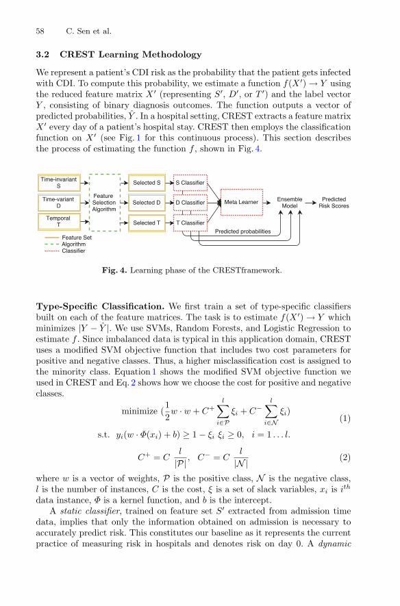
58 C. Sen et al.
3.2 CREST Learning Methodology
We represent a patient’s CDI risk as the probability that the patient gets infectedwith CDI. To compute this probability, we estimate a function f(X ′) → Y usingthe reduced feature matrix X ′ (representing S′, D′, or T ′) and the label vectorY , consisting of binary diagnosis outcomes. The function outputs a vector ofpredicted probabilities, Y . In a hospital setting, CREST extracts a feature matrixX ′ every day of a patient’s hospital stay. CREST then employs the classificationfunction on X ′ (see Fig. 1 for this continuous process). This section describesthe process of estimating the function f , shown in Fig. 4.
Fig. 4. Learning phase of the CRESTframework.
Type-Specific Classification. We first train a set of type-specific classifiersbuilt on each of the feature matrices. The task is to estimate f(X ′) → Y whichminimizes |Y − Y |. We use SVMs, Random Forests, and Logistic Regression toestimate f . Since imbalanced data is typical in this application domain, CRESTuses a modified SVM objective function that includes two cost parameters forpositive and negative classes. Thus, a higher misclassification cost is assigned tothe minority class. Equation 1 shows the modified SVM objective function weused in CREST and Eq. 2 shows how we choose the cost for positive and negativeclasses.
minimize (12w · w + C+
l∑
i∈Pξi + C−
l∑
i∈Nξi)
s.t. yi(w · Φ(xi) + b) ≥ 1 − ξi ξi ≥ 0, i = 1 . . . l.
(1)
C+ = Cl
|P| , C− = Cl
|N | (2)
where w is a vector of weights, P is the positive class, N is the negative class,l is the number of instances, C is the cost, ξ is a set of slack variables, xi is ith
data instance, Φ is a kernel function, and b is the intercept.A static classifier, trained on feature set S′ extracted from admission time
data, implies that only the information obtained on admission is necessary toaccurately predict risk. This constitutes our baseline as it represents the currentpractice of measuring risk in hospitals and denotes risk on day 0. A dynamic

CREST - Risk Prediction for Clostridium Difficile Infection 59
classifier, trained on feature set D′, constitutes a multiple-moments-in-time app-roach where the data from many moments in a patient’s stay are used as features.This approach allows us to quantify the relationship between the physiologicalstate of the patient and their CDI risk. Finally, a temporal classifier, trainedusing feature set T ′, quantifies the relationship between a patient’s state-changeand their risk, complementing the time-variant features.
Second-Order Classification. Since the three type-specific classifiers capturedifferent aspects of a patient’s health and hospital stay, we combine them toproduce a single continuous prediction based on comprehensive information. Wehypothesize that this combination method, termed second-order classification,will provide more predictive power. To evaluate this hypothesis, we merge thepredicted probability vectors from the type-specific classifiers into a new higher-order feature set Xmeta = (YS , YD, YT ). With this new feature matrix, our taskbecomes estimating a function f(Xmeta) → Y . Beyond naive methods such asmodel averaging to assign weights to the results produced by the type-specificclassifiers, we also develop a stacking-based solution. We train meta learners fus-ing SVMs with RBF and linear kernels, Random Forests, and Logistic Regressionon Xmeta to learn an integrated ensemble classifier. Henceforth, final predictionsare made by these new second-order classifier models.
4 Evaluation of CREST Framework
4.1 MIMIC-III ICU Dataset and Evaluation Settings
The MIMIC III Database [8], used to evaluate our CRESTFramework, is a pub-licly available critical care database collected from the Beth Israel DeaconessMedical Center Intensive Care Unit (ICU) between 2001 and 2012. The data-base consists of information collected from ∼45,000 unique patients and their∼58,000 admissions. Each patient’s record consists of laboratory tests, medicalprocedures, medications given, diagnoses, caregiver notes, etc.
Of the 58, 000 admissions in MIMIC, there are 1079 cases of CDI. Approx-imately half of these patients were diagnosed either before or within the first4 days of their admission. To ensure that CDI cases in our evaluation datasetare contracted during the hospital stay, we exclude patients who test positive forCDI within their first 5 days of hospitalization based on the incubation period ofCDI [4,5]. For consistency between CDI and non-CDI patients, we also excludenon-CDI patients whose hospital stay is less than 5 days. As the vast majorityof MIMIC consists of patients who do not contract CDI, we end up with anunbalanced dataset (116:1). To overcome this, we randomly subsample from thenon-CDI patients to get a 2-to-1 proportion of non-CDI to CDI patients, leavingus with 1328 patient records.
Next, we define the feature extraction window for patients. For CDI patients,it starts on the day of admission and ends n days before the CDI diagnosis,n ∈ {1, . . . , 5}. For non-CDI patients, there are a few alternatives for definingthis window. Prior research has used the discharge day as the end of the risk
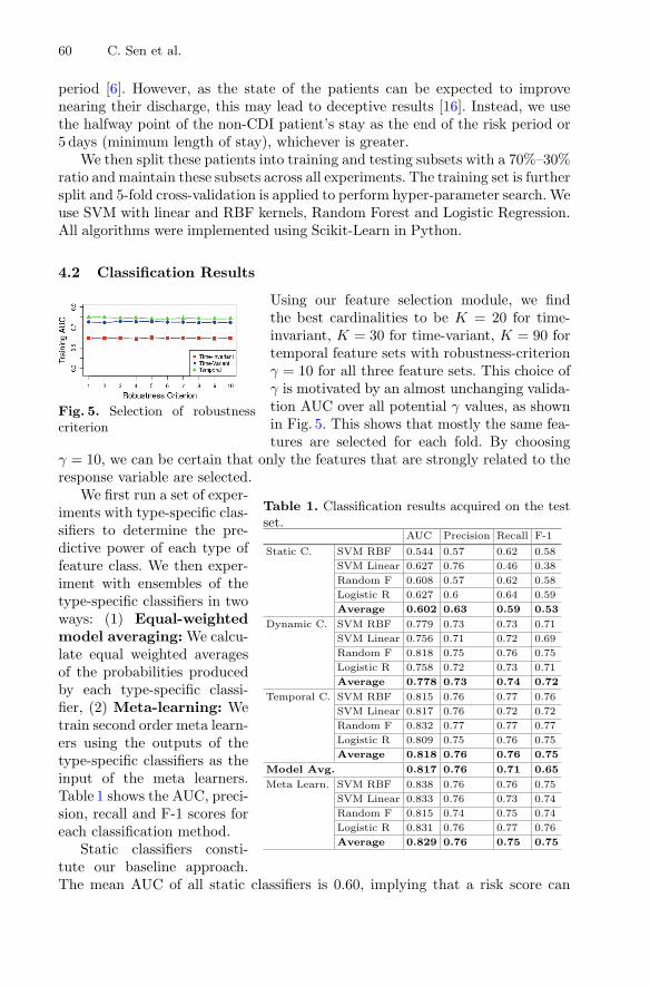
60 C. Sen et al.
period [6]. However, as the state of the patients can be expected to improvenearing their discharge, this may lead to deceptive results [16]. Instead, we usethe halfway point of the non-CDI patient’s stay as the end of the risk period or5 days (minimum length of stay), whichever is greater.
We then split these patients into training and testing subsets with a 70%–30%ratio and maintain these subsets across all experiments. The training set is furthersplit and 5-fold cross-validation is applied to perform hyper-parameter search. Weuse SVM with linear and RBF kernels, Random Forest and Logistic Regression.All algorithms were implemented using Scikit-Learn in Python.
4.2 Classification Results
Fig. 5. Selection of robustnesscriterion
Using our feature selection module, we findthe best cardinalities to be K = 20 for time-invariant, K = 30 for time-variant, K = 90 fortemporal feature sets with robustness-criterionγ = 10 for all three feature sets. This choice ofγ is motivated by an almost unchanging valida-tion AUC over all potential γ values, as shownin Fig. 5. This shows that mostly the same fea-tures are selected for each fold. By choosing
γ = 10, we can be certain that only the features that are strongly related to theresponse variable are selected.
Table 1. Classification results acquired on the testset.
AUC Precision Recall F-1
Static C. SVM RBF 0.544 0.57 0.62 0.58
SVM Linear 0.627 0.76 0.46 0.38
Random F 0.608 0.57 0.62 0.58
Logistic R 0.627 0.6 0.64 0.59
Average 0.602 0.63 0.59 0.53
Dynamic C. SVM RBF 0.779 0.73 0.73 0.71
SVM Linear 0.756 0.71 0.72 0.69
Random F 0.818 0.75 0.76 0.75
Logistic R 0.758 0.72 0.73 0.71
Average 0.778 0.73 0.74 0.72
Temporal C. SVM RBF 0.815 0.76 0.77 0.76
SVM Linear 0.817 0.76 0.72 0.72
Random F 0.832 0.77 0.77 0.77
Logistic R 0.809 0.75 0.76 0.75
Average 0.818 0.76 0.76 0.75
Model Avg. 0.817 0.76 0.71 0.65
Meta Learn. SVM RBF 0.838 0.76 0.76 0.75
SVM Linear 0.833 0.76 0.73 0.74
Random F 0.815 0.74 0.75 0.74
Logistic R 0.831 0.76 0.77 0.76
Average 0.829 0.76 0.75 0.75
We first run a set of exper-iments with type-specific clas-sifiers to determine the pre-dictive power of each type offeature class. We then exper-iment with ensembles of thetype-specific classifiers in twoways: (1) Equal-weightedmodel averaging: We calcu-late equal weighted averagesof the probabilities producedby each type-specific classi-fier, (2) Meta-learning: Wetrain second order meta learn-ers using the outputs of thetype-specific classifiers as theinput of the meta learners.Table 1 shows the AUC, preci-sion, recall and F-1 scores foreach classification method.
Static classifiers consti-tute our baseline approach.The mean AUC of all static classifiers is 0.60, implying that a risk score can
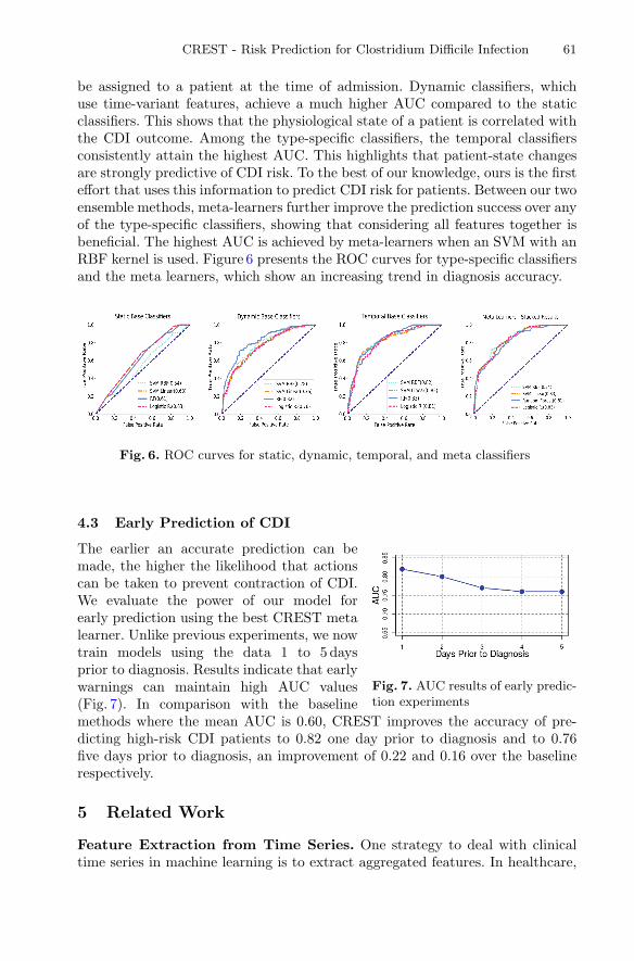
CREST - Risk Prediction for Clostridium Difficile Infection 61
be assigned to a patient at the time of admission. Dynamic classifiers, whichuse time-variant features, achieve a much higher AUC compared to the staticclassifiers. This shows that the physiological state of a patient is correlated withthe CDI outcome. Among the type-specific classifiers, the temporal classifiersconsistently attain the highest AUC. This highlights that patient-state changesare strongly predictive of CDI risk. To the best of our knowledge, ours is the firsteffort that uses this information to predict CDI risk for patients. Between our twoensemble methods, meta-learners further improve the prediction success over anyof the type-specific classifiers, showing that considering all features together isbeneficial. The highest AUC is achieved by meta-learners when an SVM with anRBF kernel is used. Figure 6 presents the ROC curves for type-specific classifiersand the meta learners, which show an increasing trend in diagnosis accuracy.
Fig. 6. ROC curves for static, dynamic, temporal, and meta classifiers
4.3 Early Prediction of CDI
Fig. 7. AUC results of early predic-tion experiments
The earlier an accurate prediction can bemade, the higher the likelihood that actionscan be taken to prevent contraction of CDI.We evaluate the power of our model forearly prediction using the best CREST metalearner. Unlike previous experiments, we nowtrain models using the data 1 to 5 daysprior to diagnosis. Results indicate that earlywarnings can maintain high AUC values(Fig. 7). In comparison with the baselinemethods where the mean AUC is 0.60, CREST improves the accuracy of pre-dicting high-risk CDI patients to 0.82 one day prior to diagnosis and to 0.76five days prior to diagnosis, an improvement of 0.22 and 0.16 over the baselinerespectively.
5 Related Work
Feature Extraction from Time Series. One strategy to deal with clinicaltime series in machine learning is to extract aggregated features. In healthcare,

62 C. Sen et al.
much work has gone into extracting features from signals such as ECG [13] orEEG [3,10] using methods such as wavelet [13,18] or Fourier [18] transforma-tions. However, EHR time series have largely being ignored. Specially designingfeature extraction techniques for EHRs in our model, we demonstrate that pre-diction accuracy increases using these features over models that do not accountfor the temporal aspects of the data.
In-hospital CDI Prediction. Recent work has begun to investigate predictionmodels for CDI. [16,17] ignore temporal dependencies in the data and reduce thiscomplex task to univariate time-series classification. [15] while combining time-variant and time-invariant data, neglect the trends in patient records. [12] usesordered pairs of clinical events to make predictions, missing longer patterns indata. In our work, we apply multivariate time series classification while capturingtemporal characteristics and long-term EHR patterns. SVMs [16,17] and LogisticRegression [6,12,14,15] are popular tools for CDI risk prediction models. Weapply a variety of models including SVM, Random Forest, Logistic Regressionand ensembles of those to produce more comprehensive results.
6 Conclusion
CREST is the first system that stratifies a patient’s infection risk on a continu-ous basis throughout their stay and is based on a novel feature extraction andcombination method. CREST has been validated for CDI risk using the MIMICDatabase. Our experimental results demonstrate that CREST can detect CDIcases with an AUC score of up to 0.84 one day before and 0.76 five days beforethe actual diagnosis. CDI is a highly contagious disease and early detection ofCDI not only greatly improves the prognosis for individual patients by enablingtimely precautions but also prevents the spread of the infection within the patientcohort. To our knowledge, this is the first work on multivariate time series clas-sification to predict the risk of CDI. We also demonstrate that our extractedtemporal synopsis features improve the AUC by 0.22 over the static classifiersand 0.04 over the dynamic classifiers.
We are in discussion with UCHealth Northern Colorado as well as Brighamand Women’s Hospital, part of the Partners Healthcare System in Massachusetts,for the potential deployment of a CREST dashboard integrated with their Elec-tronic Health Records (EPIC). This deployment will be a 4 step process, withthe work presented in this paper being the first step. The CREST framework willbe independently validated against data from ICUs at these hospitals. Successfulvalidation of CREST will lead to Step 3 - clinical usability of the EPIC-CRESTdashboard with a particular ward where daily risk scores produced by CRESTwill be utilized by the nurses to support diagnosis and early detection. Full scaledeployment will be largely dependent on the results of this clinical validationand usability study.
Acknowledgments. The authors thank Dr. Richard T. Ellison, III, the head of Infec-tion Control at UMass Memorial Medical Center, Worcester, MA, for his valuable

CREST - Risk Prediction for Clostridium Difficile Infection 63
comments that helped us understand the urgency of the CDI crisis. The authors alsothank Dr. Alfred DeMaria, Medical Director for the Bureau of Infectious Diseases atMassachusetts Public Health Department for highlighting the effects of this crisis onhealthcare systems in Massachusetts and beyond.
References
1. Centers for Disease Control and Prevention (2017). https://www.cdc.gov/media/releases/2015/p0225-clostridium-difficile.html
2. Centers for Disease Control and Prevention: Antibiotic resistance threats in theUnited States (2017). https://www.cdc.gov/drugresistance/biggestthreats.html
3. Chaovalitwongse, W.A., Prokopyev, O.A., Pardalos, P.M.: Electroencephalogram(EEG) time series classification: applications in epilepsy. Ann. Oper. Res. 148(1),227–250 (2006)
4. Cohen, S.H., et al.: Clinical practice guidelines for Clostridium difficile infectionin adults: 2010 update by the Society for Healthcare Epidemiology of America(SHEA) and the Infectious Diseases Society of America (IDSA). Infect. ControlHosp. Epidemiol. 31(05), 431–455 (2010)
5. Dubberke, E.R., et al.: Hospital-associated Clostridium difficile infection: is it nec-essary to track community-onset disease? Infect. Control Hosp. Epidemiol. 30(04),332–337 (2009)
6. Dubberke, E.R., et al.: Development and validation of a Clostridium difficile infec-tion risk prediction model. Infect. Control Hosp. Epidemiol. 32(4), 360–366 (2011)
7. Evans, C.T., Safdar, N.: Current trends in the epidemiology and outcomes ofClostridium difficile infection. Clin. Infect. Dis. 60(suppl 2), S66–S71 (2015)
8. Johnson, A.E., et al.: MIMIC-III, a freely accessible critical care database. Sci.Data 3, 160035 (2016)
9. Kuntz, J.L., et al.: Incidence of and risk factors for community-associated Clostrid-ium difficile infection: a nested case-control study. BMC Infect. Dis. 11(1), 194(2011)
10. Lemm, S., et al.: Spatio-spectral filters for improving the classification of singletrial EEG. IEEE Trans. Biomed. Eng. 52(9), 1541–1548 (2005)
11. Lessa, F.C., et al.: Burden of Clostridium difficile infection in the United States.N. Engl. J. Med. 372(9), 825–834 (2015)
12. Monsalve, M., et al.: Improving risk prediction of Clostridium difficile infectionusing temporal event-pairs. In: International Conference on Healthcare Informatics,pp. 140–149. IEEE (2015)
13. Sternickel, K.: Automatic pattern recognition in ECG time series. Comput. Meth-ods Programs Biomed. 68(2), 109–115 (2002)
14. Tanner, J., et al.: Waterlow score to predict patients at risk of developing Clostrid-ium difficile-associated disease. J. Hosp. Infect. 71(3), 239–244 (2009)
15. Wiens, J., et al.: Learning data-driven patient risk stratification models forClostridium difficile. Open Forum Infectious Diseases 1(2), ofu045 (2014)
16. Wiens, J., et al.: Learning evolving patient risk processes for C. diff colonization.In: ICML Workshop on Machine Learning from Clinical Data (2012)
17. Wiens, J., Horvitz, E., Guttag, J.V.: Patient risk stratification for hospital-associated C. diff as a time-series classification task. In: Advances in Neural Infor-mation Processing Systems, pp. 467–475 (2012)
18. Zhang, H., et. al.: Feature extraction for time series classification using disc. waveletcoefficients. In: Advances in Neural Networks. ISNN 2006, pp. 1394–1399 (2006)
DC-Prophet: Predicting Catastrophic Machine Failuresin DataCenters
You-Luen Lee1, Da-Cheng Juan2, Xuan-An Tseng1, Yu-Ting Chen2,
and Shih-Chieh Chang1(B)
1 Department of Computer Science, National Tsing Hua University, Hsinchu, [email protected], [email protected],
[email protected] Google Inc., Mountain View, CA, USA
[email protected], [email protected]
Abstract. When will a server fail catastrophically in an industrial datacenter? Isit possible to forecast these failures so preventive actions can be taken to increasethe reliability of a datacenter? To answer these questions, we have studied whatare probably the largest, publicly available datacenter traces, containing morethan 104 million events from 12,500machines. Among these samples, we observeand categorize three types of machine failures, all of which are catastrophic andmay lead to information loss, or even worse, reliability degradation of a data-center. We further propose a two-stage framework—DC-Prophet (DC-Prophetstands for DataCenter-Prophet.)—based on One-Class Support Vector Machineand Random Forest. DC-Prophet extracts surprising patterns and accurately pre-dicts the next failure of a machine. Experimental results show that DC-Prophetachieves an AUC of 0.93 in predicting the next machine failure, and a F3-score(The ideal value of F3-score is 1, indicating perfect predictions. Also, the intu-ition behind F3-score is to value “Recall” about three times more than “Precision”[12].) of 0.88 (out of 1). On average, DC-Prophet outperforms other classicalmachine learning methods by 39.45% in F3-score.
1 Introduction
“When will a server fail catastrophically in an industrial datacenter?” “Is it possibleto forecast these failures so preventive actions can be taken to increase the reliability ofa datacenter?” These two questions serve as the motivation for this work.
To meet the increasing demands for cloud computing, Internet companies such asGoogle, Facebook, and Amazon generally deploy a large fleet of servers in their data-centers. These servers bear heavy workloads and process various, diversified requests[13]. For such a high-availability computing environment, when an unexpected machinefailure happens upon a clustered partition, its workload is typically transferred toanother machine in the same cluster, which increases the possibility of other failures asa chain effect [11]. Also, this unexpected failure may cause (a) processed data loss, and(b) resource congestion due to machines being suddenly unavailable. In the worst case,these failures may paralyze a datacenter, causing an unplanned outage that requires avery high cost to recover [1]: on average $9,000/minute, and up to $17,000/minute.c© Springer International Publishing AG 2017Y. Altun et al. (Eds.): ECML PKDD 2017, Part III, LNAI 10536, pp. 64–76, 2017.https://doi.org/10.1007/978-3-319-71273-4_6

DC-Prophet: Predicting Catastrophic Machine Failures in DataCenters 65
To study machine failures in a modern datacenter, we analyze the traces from Google’sdatacenter [9,14]; the traces contain more than 104 million events generated by 12,500machines during 29 days. We observe that approximately 40% of the machines havebeen removed (due to potential failures or maintenance) at least once during this period.This phenomenon suggests that potential machine failures happen quite frequently, andcannot be simply ignored. Therefore, we want to know: given the trace of a machine, canwe accurately predict its next failure, ideally with low computing latency? If the answeris yes, the cloud scheduler (e.g., Borg [17] by Google) can take preventive actions todeal with incoming machine failures, such as by migrating tasks from the machine-to-fail to other machines. In this way, the cost of a machine failure is reduced to the veryminimum: only the cost of task migration.
While predicting the next failure of a machine seems to be a feasible and promisingsolution for improving the reliability of a datacenter, it comes with two major chal-lenges. The first challenge lies in high accuracy being required when making predic-tions, specifically for reducing false negatives. The false negatives (the machine actu-ally failed but being predicted as normal) may incur a significant recovery cost [1] andshould be avoided in Table 1. However, if the objective is set to minimize false neg-atives, the model will always predict a machine going to fail (so zero false negative),which introduces costs from false positives (the machine actually works but being pre-dicted as failed). Therefore, one major challenge of designing a model is to better tradeoff between these two costs. The second challenge is the counts between normal eventsand failure events are highly imbalanced. Among 104 million events, only 8,957 events(less than 1%) are associated with machine failures. In this case, most predictive mod-els will trivially predict every event as normal to achieve a high accuracy (higher than99%). Consequently, this event-imbalance issue is the second roadblock that needs tobe removed.
The contributions of this paper are as follows:
– We analyze probably the largest, publicly-available traces from an industrial dat-acenter, and categorize three types of machine failures: Immediate-Reboot (IR),Slow-Reboot (SR), and Forcible-Decommission (FD). The frequency and durationof each type of failures categorized by our method further match experts’ domainknowledge.
– We propose a two-stage framework:DC-Prophet that accurately predicts the occur-rence of next failure for a machine. DC-Prophet first applies One-Class SVM to fil-ter out most normal cases to resolve the event-imbalance issue, and then deploysRandom Forest to predict the type of failures that might occur for a machine.
Table 1.Misprediction issues and the associated costs
Actual: failed Actual: normal
Predicted: failed True positive (correct inference) False positive: low cost (e.g., extrarescheduling)
Predicted: normal False negative: high cost(upto $17,000/min)
True negative (correct inference)

66 Y.-L. Lee et al.
The experimental results show that DC-Prophet accurately predicts machine failuresand achieves an AUC of 0.93 and F3-score of 0.88, both on the test set.
– To understand the effectiveness of DC-Prophet, we also perform a comprehensivestudy on other widely-used machine learning methods, such as multi-class SVM,Logistic Regression, and Recurrent Neural Network. Experimental results show that,on average, DC-Prophet outperforms other methods by 39.45% in F3-score.
– Finally, we provide a practitioners’ guide for using DC-Prophet to predict the nextfailure of a machine. The latency of invoking DC-Prophet to make one predictionis less 9ms. Therefore, DC-Prophet can be seamlessly integrated into a schedulingstrategy of industrial datacenters to improve the reliability.
The remainder of this paper is organized as follows. Section 2 provides the problemdefinition, and Sect. 3 details the proposed DC-Prophet framework. Section 4 presentsthe implementation flow and experimental results, and Sect. 5 provides practitioners’guide. Finally, Sect. 6 concludes this paper.
2 Problem Definition
2.1 Google Traces Overview
The Google traces [14] consist of the activity logs from 668,000 jobs during 29 days,and each job will spawn one or more tasks to be executed in a 12,500-machine cluster.For each machine, the traces record (a) computing resources consumed by all the tasksrunning on that machine, and (b) its machine state. Both resource consumption andmachine states are recorded with associated time interval of one-microsecond (1 µs)resolution.
We focus on the usage measurements of six types of resources: (a) CPU usage, (b)disk I/O time, (c) disk space usage, (d) memory usage, (e) page cache, and (f) mem-ory access per instruction. All these measurements are normalized by their respectivemaximum values and thus range from 0 to 1. In this work, the average and peak valuesduring the time interval of 5min are also calculated for each usage–the interval of 5minis typically used to report the measured resource footprint of a task in Google’s data-center [14]. Furthermore, resource usages at minute-level provide a more macro viewof a machine status [8]. We use xr,t to denote the average usage of resource type r attime interval t; similarly, mr,t represents the peak usage. Both xr,t and mr,t are used toconstruct the training dataset, with further details provided in Sect. 2.4.
In addition, Google traces also contain three types of events to determine machinestates: ADD, REMOVE, and UPDATE [14]. In this work, we treat each REMOVE eventas an anomaly that could potentially be a machine failure. Detailed analyses are furtherprovided in Sect. 2.3.
2.2 Problem Formulation
The problem of predicting the next machine failure is formulated as follows:problem 1 (Categorize catastrophic failures). Given the traces of machine events,
categorize the type of each machine failure at time interval t (denoted as yt).

DC-Prophet: Predicting Catastrophic Machine Failures in DataCenters 67
problem 2 (Forecast catastrophic failures). Given the traces of resource usages—denoted as xr,t and mr,t—up to time interval τ − 1, forecast the next failure and itstype at time interval τ (denoted as yτ ) for each machine. Mathematically, this problemcan be expressed as:
yτ = f(xr,t,mr,t), t = 1 to τ − 1, r ∈ resources (1)
where xr,t and mr,t represent the respective average and peak usage of resource r attime interval t.
We use Fig. 1 to better illustrate the concept in Eq. (1), specifically the temporalrelationship among yτ , xr,t and mr,t for t = 1 to τ − 1. One goal here is to find afunction f that takes xr,t and mr,t as inputs to predict yτ .
Fig. 1. Relationship among yτ , xr,t and mr,t for t = 1 to τ − 1.
2.3 Machine-Failure Analyses
Throughout the 29-day traces, we find a total of 8,957 potential machine failures fromthe REMOVE events, and Fig. 2(a) illustrates the rank-frequency of these failures. Thedistribution is power-law-like and heavily skewed: the top-ranked machines failed morethan 100 times, whereas the majority of machines (3,397 machines) failed only once.Overall, about 40% (out of 12,500) machines have been removed at least once. Wefurther notice that the resource usages of these most frequently-failing machines areall zeros, indicating a clear abnormal behavior. These machines seem being marked asunavailable internally [2], and hence are apparent anomalies. They are excluded fromthe analysis later on.
Observation 1. Most frequently-failing machines have failed more than 100 times over29 days, with usages of all resource types being zero.
To categorize the type of a failure, we further analyze its duration which is cal-culated by the time difference between the REMOVE and the following ADD event.Figure 2(b) illustrates the distribution of durations for all machine failures. The fail-ure duration can vary a lot, ranging from few minutes, to few hours, to never back—amachine is never added back to the cluster after its REMOVE event. Furthermore, three“peaks” can be observed in failure durations: ≈16min, ≈2 h, and never back.
Observation 2. Three “peaks” in the histogram of failure durations correspond to≈16min, ≈2 h, and never back.
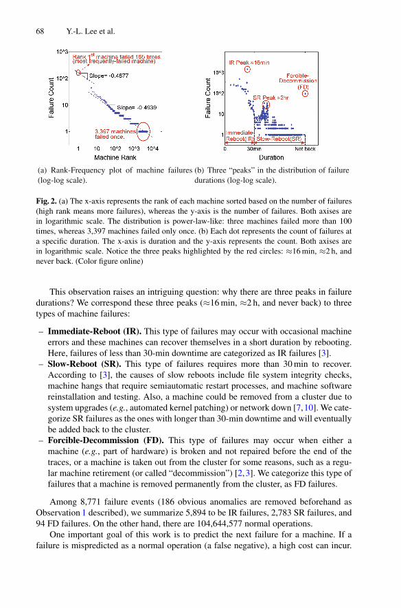
68 Y.-L. Lee et al.
(a) Rank-Frequency plot of machine failures(log-log scale).
(b) Three “peaks” in the distribution of failuredurations (log-log scale).
Fig. 2. (a) The x-axis represents the rank of each machine sorted based on the number of failures(high rank means more failures), whereas the y-axis is the number of failures. Both axises arein logarithmic scale. The distribution is power-law-like: three machines failed more than 100times, whereas 3,397 machines failed only once. (b) Each dot represents the count of failures ata specific duration. The x-axis is duration and the y-axis represents the count. Both axises arein logarithmic scale. Notice the three peaks highlighted by the red circles: ≈16min, ≈2 h, andnever back. (Color figure online)
This observation raises an intriguing question: why there are three peaks in failuredurations? We correspond these three peaks (≈16min, ≈2 h, and never back) to threetypes of machine failures:
– Immediate-Reboot (IR). This type of failures may occur with occasional machineerrors and these machines can recover themselves in a short duration by rebooting.Here, failures of less than 30-min downtime are categorized as IR failures [3].
– Slow-Reboot (SR). This type of failures requires more than 30min to recover.According to [3], the causes of slow reboots include file system integrity checks,machine hangs that require semiautomatic restart processes, and machine softwarereinstallation and testing. Also, a machine could be removed from a cluster due tosystem upgrades (e.g., automated kernel patching) or network down [7,10]. We cate-gorize SR failures as the ones with longer than 30-min downtime and will eventuallybe added back to the cluster.
– Forcible-Decommission (FD). This type of failures may occur when either amachine (e.g., part of hardware) is broken and not repaired before the end of thetraces, or a machine is taken out from the cluster for some reasons, such as a regu-lar machine retirement (or called “decommission”) [2,3]. We categorize this type offailures that a machine is removed permanently from the cluster, as FD failures.
Among 8,771 failure events (186 obvious anomalies are removed beforehand asObservation 1 described), we summarize 5,894 to be IR failures, 2,783 SR failures, and94 FD failures. On the other hand, there are 104,644,577 normal operations.
One important goal of this work is to predict the next failure for a machine. If afailure is mispredicted as a normal operation (a false negative), a high cost can incur.

DC-Prophet: Predicting Catastrophic Machine Failures in DataCenters 69
For example, the user jobs can be killed unexpectedly, leading to processed data loss.If these failures can be predicted accurately in advance, the cloud/cluster scheduler canperform preventive actions such as rescheduling jobs to another available machine tomitigate the negative impacts. Compared to the cost incurred from false negatives, i.e.,mispredicting a failure as a normal operation, the cost of “misclassifying” one failuretype as another is relatively low. Still, if the right types of failures can be correctlypredicted, the cloud/cluster scheduler can plan and arrange the computing resourcesaccordingly.
2.4 Construct Training Dataset
We model the prediction of the next machine failure from Eq. (1) as a multi-class clas-sification and construct the training dataset accordingly. Each instance in the datasetconsists of a label yτ that represents the failure type at time interval τ , and a set of pre-dictive features x (or called a feature vector) extracted from the resource usages up totime interval τ − 1.
The type of a label yτ is determined based on the failure duration described inSect. 2.3. If there is no machine failure at time interval τ , label yτ is marked as “normaloperation.” Therefore, we defined yτ ∈ {0, 1, 2, 3}, which represents normal operation,IR, SR, and FD, respectively.
For the predictive features x, we leverage both the average xr,t and peak valuesmr,t
of six resource types as mentioned in Sect. 2.1. Now the question is: how to select thenumber of time intervals needed to be included in the dataset for an accurate prediction?We propose to calculate the partial autocorrelation to determine the number of intervals,or called “lags” in time series, to be included in the predictive features x. Assume targetinterval is τ , the interval with “one lag” will be τ − 1 (and the interval with two lagswill be τ − 2, etc.). Partial autocorrelation is a type of conditional correlation betweenxr,τ and xr,t, with the linear dependency of xr,t+1 to xr,τ−1 removed [5]. Since thepartial autocorrelation can be treated as “the correlation between xr,τ and xr,t, withother linear dependency removed,” it suggests how many time intervals (or lags) shouldbe included in the predictive features.
Figure 3(a) illustrates the partial autocorrelation of the CPU usage on one machine,and Fig. 3(b) represents the histogram of partial autocorrelations with certain lags. Boththe figures show statistical significance. Notice in general, after 6 lags (30min), theresource usages are less relevant.
Observation 3. Resource usages from 30min ago are less relevant to the current usagein terms of partial autocorrelation.
Based on this observation, we include resource usages within 30min as featuresto predict failure type yτ . In other words, 6 time intervals (lags) are selected for bothxr,t and mr,t to construct the predictive features xt. Specifically, xt = {xr,t,mr,t},r ∈ resources and t = τ − j where j = 1 to 6. Therefore, x has 2 (average and peakusages) × 6 (number of resources) × 6 (intervals) = 72 predictive features.
Now we have constructed the training dataset, and are ready to proceed to the pro-posed framework. For conciseness, in the rest of this paper each instance will be pre-sented as (y,x) instead of (yτ ,xt) with t = τ − 1, ..., τ − 6.

70 Y.-L. Lee et al.
(a) Partial autocorrelation of CPU us-age.
(b) Histogram of statistically-significant partial autocorrelationson all machines.
Fig. 3. (a) Lags of 1, 2, 3, 5 and 6 correlate with lag 0, i.e., xcpu,τ , and these correlations arestatistically significant. (b) For each machine, partial autocorrelations with up to 10 lags arecalculated; only statistically-significant lags are reported for plotting this histogram. Notice ingeneral, after 6 lags (or time intervals) the resource usages are less relevant—only few machinesreport partial autocorrelations with 6+ lags that are statistically significant.
3 Methodology
3.1 Overview: Two-Stage Framework
Begin immediately, we illustrate the proposed two-stage framework with Fig. 4. Inthe first stage, One-Class Support Vector Machine (OCSVM) is deployed for anom-aly detection. All the detected anomalies are then sent to Random Forest for multi-classclassification. Mathematically, DC-Prophet can be expressed as a two-stage framework:
f(x) = g(x) · h(x) ={0, if g(x) = 0h(x), if g(x) = 1 (2)
where g(·) ∈ {0, 1} is OCSVM and h(·) ∈ {0, 1, 2, 3} is Random Forest. For anincoming instance x, it will first be sent to g(·) for anomaly detection. If x is detected
Fig. 4. Flow chart of DC-Prophet: two-stage framework. At the first stage, a sample x is sent toOne-Class SVM g(·) for anomaly detection (i.e., potential machine failure or normal operation).If x is classified as a potential machine failure, then this sample will be further sent to RandomForest h(·) for multi-class (IR, SR, FD, or normal) classification.

DC-Prophet: Predicting Catastrophic Machine Failures in DataCenters 71
as an anomaly, i.e., a potential machine failure, it will be further sent to h(·) for multi-class classification.
In Google traces, the distribution of four label types is extremely unbalanced: 104millions of normal cases versus 8,771 failures that are treated as anomalies (includingall three types of failures). Therefore, OCSVM is applied to filter out most of normaloperations and detect anomalies, i.e., potential machine failures. Without doing so, clas-sifiers will be swamped by normal operations, learn only the “normal behaviors,” andchoose to ignore all the failures. This will cause significant false negatives as mentionedin Table 1 since most machine failures are mispredicted as normal operations.
3.2 One-Class SVM
One-class SVM (OCSVM) is often applied for novelty (or outlier) detection [4] anddeployed as g(·) in DC-Prophet. OCSVM is trained on instances that have only oneclass, which is the “normal” class; given a set of normal instances, OCSVM detects thesoft boundary of the set, for classifying whether a new incoming instance belongs tothat set (i.e., “normal”) or not. Specifically, OCSVM computes a non-linear decisionboundary, using appropriate kernel functions; in this work, radial basis function (RBF)kernel is used [15]. Equation (3) below show how OCSVM makes an inference:
g(x) ={1, g(x) ≥ 00, g(x) < 1 where g(x) = 〈w, φ(x)〉 + ρ (3)
where w and ρ are learnable weights that determine the decision boundary, and thefunction φ(·)maps the original feature(s) into a higher dimensional space, to determinethe optimal decision boundary. By further modifying the hard-margin SVM to toleratesome misclassifications, we have:
minw,ρ
12||w||22 + C
n∑i
ξi − ρ
s.t. g(xi) = 〈w, φ(xi)〉 − ρ ≤ ξi
ξi ≥ 0 (4)
where ξi represents the classification error of ith sample, and C represents the weightthat trades off between the maximum margin and the error-tolerance.
3.3 Random Forest
In the second stage of DC-Prophet, Random Forest [6] is used for multi-class clas-sification. Random Forest is a type of ensemble model that leverages the classificationoutcomes from several (sayB) decision trees for making the final classification. In otherwords, Random Forest is an ensemble of B trees {T1(x), ..., TB(x)}, where x is thevector of predictive features described in Sect. 2.4. This ensemble of B trees predicts Boutcomes {y1 = T1(x), ..., yB = TB(x)}. Then the outcomes of all trees are aggregatedfor majority voting, and the final prediction y is made based on the highest (i.e., most

72 Y.-L. Lee et al.
popular) vote. Empirically, Random Forest is robust to overfitting and achieves a veryhigh accuracy.
Given a dataset of n instances {(x1, y1), ..., (xn, yn)}, the training procedure ofRandom Forest is as follows:
1. Randomly sample the training data {(x1, y1), ..., (xn, yn)}, and then draw n samplesto form a bootstrap batch.
2. Grow a decision tree from the bootstrap batch using the Decision Tree ConstructionAlgorithm [4].
3. Repeat the above two steps until the whole ensemble of B trees {T1(x), ..., TB(x)}are grown.
After Random Forest is grown, along with the OCSVM in the first stage, DC-Prophet is ready for predicting the type of a machine failure.
4 Experimental Results
4.1 Experimental Setup
To best compare the proposed DC-Prophet with other machine learning models, wemanage to search for the best hyperparameters by using 5-fold cross-validation for allthe methods. Then the accuracy of each method is evaluated on the test set. All theexperiments are conducted via MATLAB, running on Intel I5 processor (3.20GHz)with 16GB of RAM.
For the evaluation metrics, we report Precision, Recall, F -score, and AUC (areaunder ROC curve) to provide a comprehensive study on the performance evaluation fordifferent models. F -score is defined as:
Fβ = (1 + β2)Precision ∗ Recall
(β2 ∗ Precision) + Recall(5)
where β is the parameter representing the relative importance between Recall andPrecision [16]. In this work, β is selected to be 3, which means Recall is approxi-mately three times more important than Precision. Since the false negative (machinefailure mispredicted as normal event) is much more costly as mentioned in Table 1, F3-score is used as the main criterion to select the best framework for predicting failuretypes.
4.2 Results Summary
Table 2 shows the experimental results from different methods. We calculate and reportPrecision, Recall, F3-score and AUC for comprehensive comparisons. The resultsdemonstrate that the two-stage algorithms have better performance on both F3-scoreand AUC. It also shows that using One-Class SVM for anomaly detection as the firststage is necessary. Among 8,771 failures, One-Class SVM only mispredicts 11 failuresas normal events, which serves as an excellent filter. Furthermore, our proposed frame-work, DC-Prophet, which combines One-Class SVM and Random Forest, has the bestF3-score and AUC among all the two-stage methods.
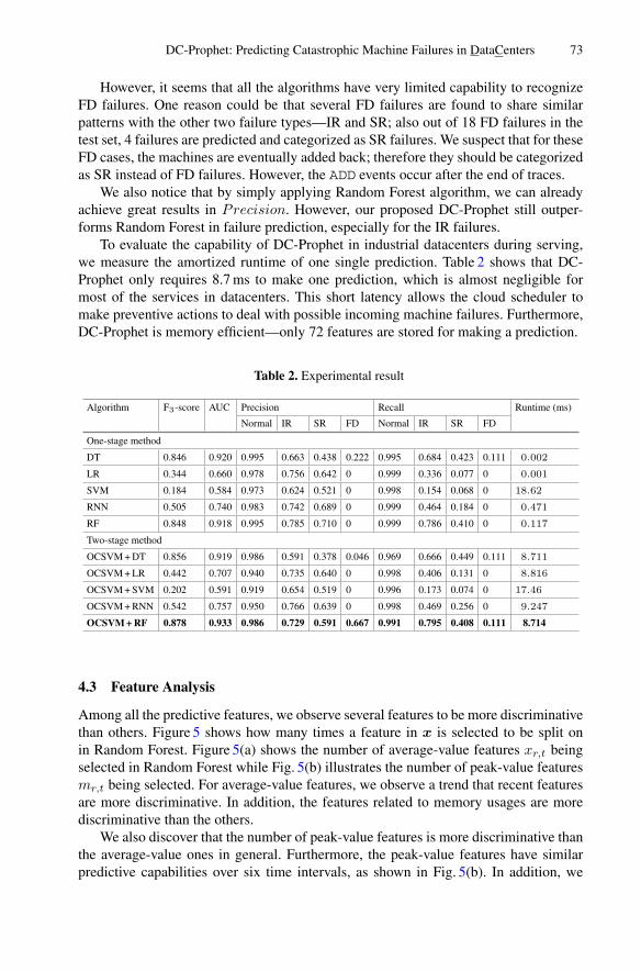
DC-Prophet: Predicting Catastrophic Machine Failures in DataCenters 73
However, it seems that all the algorithms have very limited capability to recognizeFD failures. One reason could be that several FD failures are found to share similarpatterns with the other two failure types—IR and SR; also out of 18 FD failures in thetest set, 4 failures are predicted and categorized as SR failures. We suspect that for theseFD cases, the machines are eventually added back; therefore they should be categorizedas SR instead of FD failures. However, the ADD events occur after the end of traces.
We also notice that by simply applying Random Forest algorithm, we can alreadyachieve great results in Precision. However, our proposed DC-Prophet still outper-forms Random Forest in failure prediction, especially for the IR failures.
To evaluate the capability of DC-Prophet in industrial datacenters during serving,we measure the amortized runtime of one single prediction. Table 2 shows that DC-Prophet only requires 8.7ms to make one prediction, which is almost negligible formost of the services in datacenters. This short latency allows the cloud scheduler tomake preventive actions to deal with possible incoming machine failures. Furthermore,DC-Prophet is memory efficient—only 72 features are stored for making a prediction.
Table 2. Experimental result
Algorithm F3-score AUC Precision Recall Runtime (ms)
Normal IR SR FD Normal IR SR FD
One-stage method
DT 0.846 0.920 0.995 0.663 0.438 0.222 0.995 0.684 0.423 0.111 0.002
LR 0.344 0.660 0.978 0.756 0.642 0 0.999 0.336 0.077 0 0.001
SVM 0.184 0.584 0.973 0.624 0.521 0 0.998 0.154 0.068 0 18.62
RNN 0.505 0.740 0.983 0.742 0.689 0 0.999 0.464 0.184 0 0.471
RF 0.848 0.918 0.995 0.785 0.710 0 0.999 0.786 0.410 0 0.117
Two-stage method
OCSVM+DT 0.856 0.919 0.986 0.591 0.378 0.046 0.969 0.666 0.449 0.111 8.711
OCSVM+LR 0.442 0.707 0.940 0.735 0.640 0 0.998 0.406 0.131 0 8.816
OCSVM+SVM 0.202 0.591 0.919 0.654 0.519 0 0.996 0.173 0.074 0 17.46
OCSVM+RNN 0.542 0.757 0.950 0.766 0.639 0 0.998 0.469 0.256 0 9.247
OCSVM+RF 0.878 0.933 0.986 0.729 0.591 0.667 0.991 0.795 0.408 0.111 8.714
4.3 Feature Analysis
Among all the predictive features, we observe several features to be more discriminativethan others. Figure 5 shows how many times a feature in x is selected to be split onin Random Forest. Figure 5(a) shows the number of average-value features xr,t beingselected in Random Forest while Fig. 5(b) illustrates the number of peak-value featuresmr,t being selected. For average-value features, we observe a trend that recent featuresare more discriminative. In addition, the features related to memory usages are morediscriminative than the others.
We also discover that the number of peak-value features is more discriminative thanthe average-value ones in general. Furthermore, the peak-value features have similarpredictive capabilities over six time intervals, as shown in Fig. 5(b). In addition, we

74 Y.-L. Lee et al.
Fig. 5. Counts of features selected by Random Forest : (a) shows the number of average-valuefeatures xr,t being selected. We observe a trend that more recent features are more discriminative.(b) shows the number of peak-value features mr,t being selected. (Color figure online)
observe that the peak usage of local disk is an important feature for predicting machinefailures (see red circles in Fig. 5(b)).
5 Practitioners’ Guide
Here we provide the practitioners’ guide to applying DC-Prophet for forecastingmachine failures in a datacenter:
– Construct Training Dataset: Given the traces of machines in a datacenter, extractabnormal events representing potential machine failures, and determine their typesbased on the observations in Sect. 2.3 for obtaining label y. Then calculate the partialautocorrelation for each resource measurement (e.g., CPU usage, disk I/O time, etc.)to determine the number of time intervals (or lags) to be included as the predictivefeatures x.
– One-Class SVM: After constructing the dataset of (y, x), train OCSVM with theinstances labeled as “normal” only, and find the best hyperparameters via grid-searchand cross-validation.
– Random Forest: After OCSVM is trained, remove the instances detected as nor-mal from the training dataset. Use the rest of dataset (treated as anomalies) to trainRandom Forest. Choose the number of trees in the ensemble and optimize it bycross-validation.
After both components of DC-Prophet are trained, each new incoming instance willfollow the flow in Fig. 4 for failure prediction. Thanks to DC-Prophet’s low latency(8.71ms per invocation), it can be used for both (a) offline analysis in other similar dat-acenters, and (b) serving as a failure predictor integrated into a cloud/cluster scheduler,with training via historical data offline.
DC-Prophet: Predicting Catastrophic Machine Failures in DataCenters 75
6 Conclusion
In this paper, we propose DC-Prophet: a two-stage framework for forecasting machinefailures. Thanks to DC-Prophet, we now can answer the two motivational questions:“When will a server fail catastrophically in an industrial datacenter?” “Is it possible toforecast these failures so preventive actions can be taken to increase the reliability ofa datacenter?” Experimental results show that DC-Prophet accurately predicts machinefailures and achieves an AUC of 0.93 and F3-score of 0.88. Finally, a practitioners’guide is provided for deploying DC-Prophet to predict the next failure of a machine.The latency of invoking DC-Prophet to make one prediction is less 9ms, and therecan be seamlessly integrated into the scheduling strategy of industrial datacenters toimprove the reliability.
References
1. 2016 cost of data center outages report. https://goo.gl/OeNM4U2. Google cluster data - discussions (2011). https://groups.google.com/forum/#!forum/
googleclusterdata-discuss3. Barroso, L.A., Clidaras, J., Holzle, U.: The datacenter as a computer: an introduction to the
design of warehouse-scale machines. Synth. Lect. Comput. Archit. 8(3), 1–154 (2013)4. Bishop, C.: Pattern Recognition and Machine Learning. Information Science and Statistics.
Springer, New York (2006)5. Box, G.E., Jenkins, G.M., Reinsel, G.C., Ljung, G.M.: Time Series Analysis: Forecasting
and Control. Wiley, New York (2015)6. Breiman, L.: Random forests. Mach. Learn. 45(1), 5–32 (2001)7. Chen, X., Lu, C.-D., Pattabiraman, K.: Failure analysis of jobs in compute clouds: a Google
cluster case study. In: 2014 IEEE 25th International Symposium on Software ReliabilityEngineering, pp. 167–177. IEEE (2014)
8. Guan, Q., Fu, S.: Adaptive anomaly identification by exploring metric subspace in cloudcomputing infrastructures. In: 2013 IEEE 32nd International Symposium on Reliable Dis-tributed Systems (SRDS), pp. 205–214. IEEE (2013)
9. Juan, D.-C., Li, L., Peng, H.-K., Marculescu, D., Faloutsos, C.: Beyond poisson: modelinginter-arrival time of requests in a datacenter. In: Tseng, V.S., Ho, T.B., Zhou, Z.-H., Chen,A.L.P., Kao, H.-Y. (eds.) PAKDD 2014. LNCS (LNAI), vol. 8444, pp. 198–209. Springer,Cham (2014). https://doi.org/10.1007/978-3-319-06605-9 17
10. Liu, Z., Cho, S.: Characterizing machines and workloads on a Google cluster. In: 2012 41stInternational Conference on Parallel Processing Workshops, pp. 397–403. IEEE (2012)
11. Miller, T.D., Crawford Jr., I.L.: Terminating a non-clustered workload in response to a failureof a system with a clustered workload. US Patent 7,653,833, 26 January 2010
12. Powers, D.M.: Evaluation: from precision, recall and f-measure to ROC, informedness,markedness and correlation. J. Mach. Learn. Technol. 2(1), 37–63 (2011)
13. Reiss, C., Tumanov, A., Ganger, G.R., Katz, R.H., Kozuch, M.A.: Heterogeneity and dynam-icity of clouds at scale: Google trace analysis. In: SOCC, p. 7. ACM (2012)
14. Reiss, C., Wilkes, J., Hellerstein, J.L.: Google cluster-usage traces: format + schema. Tech-nical report, Google Inc., Mountain View, CA, USA, version 2.1, November 2011. https://github.com/google/cluster-data. Accessed 17 Nov 2014
15. Scholkopf, B., Sung, K.-K., Burges, C.J., Girosi, F., Niyogi, P., Poggio, T., Vapnik, V.: Com-paring support vector machines with Gaussian kernels to radial basis function classifiers.IEEE Trans. Signal Process. 45(11), 2758–2765 (1997)

76 Y.-L. Lee et al.
16. van Rijsbergen, C.: Information Retrieval, 2nd edn. Butterworths, London (1979)17. Verma, A., Pedrosa, L., Korupolu, M., Oppenheimer, D., Tune, E., Wilkes, J.: Large-scale
cluster management at Google with Borg. In: Proceedings of the Tenth European Conferenceon Computer Systems, p. 18. ACM (2015)
Disjoint-Support Factors and SeasonalityEstimation in E-Commerce
Abhay Jha(B)
Facebook, Inc., Menlo Park, CA, [email protected]
Abstract. Successful inventory management in retail entails accuratedemand forecasts for many weeks/months ahead. Forecasting models useseasonality: recurring pattern of sales every year, to make this forecast. Ine-commerce setting, where the catalog of items is much larger than brickand mortar stores and hence includes a lot of items with short history, itis infeasible to compute seasonality for items individually. It is customaryin these cases to use ideas from factor analysis and express seasonality bya few factors/basis vectors computed together for an entire assortmentof related items. In this paper, we demonstrate the effectiveness of choos-ing vectors with disjoint support as basis for seasonality when dealingwith a large number of short time-series. We give theoretical results oncomputation of disjoint support factors that extend the state of the art,and also discuss temporal regularization necessary to make it work onwalmart e-commerce dataset. Our experiments demonstrate a markedimprovement in forecast accuracy for items with short history.
1 Introduction
Seasonality refers to patterns in a time-series that repeat themselves every sea-son. For example, retail sales always increase in November, unemployment dropsin December, temperature increases in summer. In general, one is interested infinding the smooth periodic pattern underlying a long univariate time-serieswhich has data for many past seasons. This reduces to some form of regres-sion of observation on the season, for e.g., day/week, as exemplified in a lot oftime-series literature [1–3].
In this paper, we will focus on finding the weekly seasonality of sales onan annual basis. We focus on e-commerce, which is a decidedly different andarguably more challenging task, because the assortment of items is larger andmore dynamic– this implies there is a large number of time-series and most ofthem do not have enough data for even one year. This make the traditionalapproach of regression infeasible, since we cannot estimate a 52 week seasonalityfrom, say only 6 weeks of sales. The problem in this domain is more suited tofactor analysis and matrix factorization techniques, which have been successfullyused for imputation in other scenarios with a lot of missing data [4]. In this
Work done while the author was at @WalmartLabs.
c© Springer International Publishing AG 2017Y. Altun et al. (Eds.): ECML PKDD 2017, Part III, LNAI 10536, pp. 77–88, 2017.https://doi.org/10.1007/978-3-319-71273-4_7
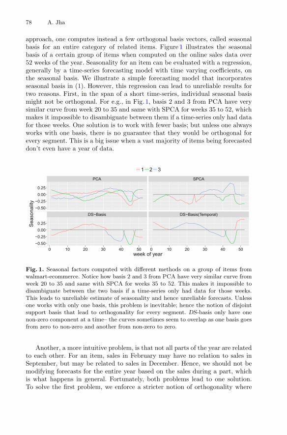
78 A. Jha
approach, one computes instead a few orthogonal basis vectors, called seasonalbasis for an entire category of related items. Figure 1 illustrates the seasonalbasis of a certain group of items when computed on the online sales data over52 weeks of the year. Seasonality for an item can be evaluated with a regression,generally by a time-series forecasting model with time varying coefficients, onthe seasonal basis. We illustrate a simple forecasting model that incorporatesseasonal basis in (1). However, this regression can lead to unreliable results fortwo reasons. First, in the span of a short time-series, individual seasonal basismight not be orthogonal. For e.g., in Fig. 1, basis 2 and 3 from PCA have verysimilar curve from week 20 to 35 and same with SPCA for weeks 35 to 52, whichmakes it impossible to disambiguate between them if a time-series only had datafor those weeks. One solution is to work with fewer basis; but unless one alwaysworks with one basis, there is no guarantee that they would be orthogonal forevery segment. This is a big issue when a vast majority of items being forecasteddon’t even have a year of data.
DS−Basis DS−Basis(Temporal)
PCA SPCA
0 10 20 30 40 50 0 10 20 30 40 50
−0.50−0.25
0.000.25
−0.50−0.25
0.000.25
week of year
Sea
sona
lity
1 2 3
Fig. 1. Seasonal factors computed with different methods on a group of items fromwalmart-ecommerce. Notice how basis 2 and 3 from PCA have very similar curve fromweek 20 to 35 and same with SPCA for weeks 35 to 52. This makes it impossible todisambiguate between the two basis if a time-series only had data for those weeks.This leads to unreliable estimate of seasonality and hence unreliable forecasts. Unlessone works with only one basis, this problem is inevitable; hence the notion of disjointsupport basis that lead to orthogonality for every segment. DS-basis only have onenon-zero component at a time– the curves sometimes seem to overlap as one basis goesfrom zero to non-zero and another from non-zero to zero.
Another, a more intuitive problem, is that not all parts of the year are relatedto each other. For an item, sales in February may have no relation to sales inSeptember, but may be related to sales in December. Hence, we should not bemodifying forecasts for the entire year based on the sales during a part, whichis what happens in general. Fortunately, both problems lead to one solution.To solve the first problem, we enforce a stricter notion of orthogonality where

Disjoint-Support Factors and Seasonality Estimation in E-Commerce 79
every segment of two vectors is orthogonal; it can be shown to be equivalent tothem having Disjoint Support (DS). Figure 1 illustrates DS-basis. They solve thesecond problem as well by segmenting the year into different weeks which exhibita distinct behavior. However, with disjoint supports there is only one curve tomodel the variation during any part of the year, which is not always true whenone considers a large group of possibly unrelated items. So, one way of viewingDS-basis is as a strong regularizer imposed on a group of items which forces theirsales to follow one curve during the seasonal events. This is not recommendedfor the entire catalog together, but for groups of related items in the cataloghierarchy.
In this paper, we will study how to compute DS-basis, both with theoreticalresults, and practical lessons learned in applying it at walmart e-commerce. Weshow that DS-basis for a low rank matrix can be computed in polynomial time.Our proof relies on bounding the number of regions of a low rank hyperplanearrangement. For general matrices, we show that the problem is NP-hard, witha reduction from graph coloring. We also give a constant factor approximationalgorithm, and prove hardness of approximation results.
When applying this technique at Walmart E-Commerce, we observed multi-ple anomalies in the basis computed, compared to our domain knowledge. Thisis because real world datasets are noisy and there are many factors that leadto variation in sales that cannot be accounted for. We propose certain temporalregularizations that can overcome this noise, by exploiting the fact that our datais a time-series. Computing the basis with these regularization entails learningin Switching State Space Models which is often done with moment-matchingKalman Filters [5]. We propose an alternative faster approach that leveragesforward-backward algorithm for estimation in HMM, to achieve the same accu-racy, in less execution time.
Our experiments demonstrate that forecast accuracy is markedly improvedfor items with short history. Further empirical evaluations are done on a syntheticdataset for a more detailed comparison. This paper is organized as follows: Sect. 2gives some background and discusses the related work, and we describe ourapproach along with the computational complexity of the problem in Sect. 3, andSect. 4, which focuses on a more general problem with temporal regularizations.Section 5 has the empirical evaluation of our approach conducted on walmarte-commerce, and a synthetic data.
2 Background and Related Work
Related Work. The general approach of estimating seasonality is by decom-posing the time-series into mean, trend and seasonal components, see [6] foran example. The seasonal component can be modeled as a cyclic/periodic com-ponent in the form of a triginometric series. However, because of leap years,seasonality in our setting is not the same as periodicity. However, it can stillbe computed by a regression of observation with the week number– but as wealready pointed out this approach does not work for short series. One could still

80 A. Jha
use hierarchical regressions [7] commonly used in panel data– in this approachwe would use item catalog to specify a hierarchy of items, however this approachdoes not scale well to large datasets we use. This is inherent to the methoditself because of computations involving large covariance matrices. Also, gener-ally some sort of clustering is needed before applying these methods as describedin [8].
The application of forecasting to settings like ours is relatively new, butthe idea of seasonal factors is not new and has been investigated by others aswell. For e.g., [9,10], explore Non-Negative Matrix Factorization (NMF), andPrincipal Component Analysis (PCA) respectively. In this paper, we are focusednot on the particulars of whether factors be non-negative, or sparse or smooth;instead we are proposing that they have disjoint support which is an orthogonalidea that can be used along with each of these approaches. We build upon PCAsince it is the most common way of estimating factors.
Notation. Given a vector v, we denote coordinate i by vi. For a matrix M , wedenote row i and column j with M [i, j]; column i with mi. We say vectors u,v have disjoint support iff ∀i, uivi = 0. The reason we are interested in them isbecause they ensure orthogonality of arbitrary segments of u, v. For a naturalnumber n, [n] denotes the set {1, 2, . . . , n}.
Forecasting with Seasonal Basis. Since this paper is about computing season-ality, we won’t delve into the forecasting models, but we do want to illustrate howseasonality is incorporated in forecasting to motivate the problem. The followingis a simple univariate local-level model which has a mean component μ and a sea-sonality component that is expressed by seasonal basis that form rows of H.
yt = μt + hTs(t)αt + εt εt ∼ N(0, σ2),
μt = μt−1 + ηt ηt ∼ N(0, λμσ2),
αt = αt−1 + ωt ωt ∼ N(0, λωσ2Ik) (1)
where s(t) denotes the season at time t. For e.g., if we are making weekly forecastsit will be between 1 to 52, for daily forecasts it would vary from 1 to 365. Onecould add more components to the model like trend, and include price andcalendar effects. Furthermore, this could be generalized to a multivariate model.
Problem Statement. Let Y be an n × p sales matrix, where p is the number ofseasons, for e.g. p = 52 in Fig. 1. We will assume that rows of Y are centered totake out the effect of mean. Also, note that Y can have missing values. Our goal inthis paper is to express Y as WH, where W is an n×k matrix of basis coefficients,and H is a k × p matrix whose rows have disjoint support and HHT = I, thatminimize ‖Y − WH‖2F , which is same as maximizing Tr
(HY T Y HT
). Note that
the constraint HHT = I is just for uniqueness; we could also enforce WT W = Iinstead– depending on the algorithm one constraint is preferred over the other.We will extend the problem further by adding some temporal constraints on therows of H in Sect. 4. k is typically a small number, and hence would be assumed tobe a bounded constant when stating complexity results throughout this paper.

Disjoint-Support Factors and Seasonality Estimation in E-Commerce 81
Input: Yn×p = Un×rVr×p, #factorsk
Output: W , HZr×k ← variables from a rk-D space
S ← ⋃1≤i≤p
⋃1≤j1<j2≤k{vT
i zj1 ±vT
i zj2 = 0 }r(S) ← regions of arrangement Sopt ← 0for regions ∇ ∈ r(S) do
Support(i) ← argmaxj
(vT
i zj
)2,
∀i ∈ [p]Mj ← columns of Y withsupport j, ∀j ∈ [k]
currOpt ← ∑ki=1 σ2
1(Mi)if currOpt > opt then
opt ← currOptH ← right singular vectorsof Mi, i = 1..k
end
end
W ← Y HT
return W , HAlgorithm 1. Computing DS-basisfor a low rank matrix
Fig. 2. Consider functions 1.x2, 2.y2, 3.(x + y)2. The above arrangement of linespartitions 2D-space into regions which areannotated with 1/2/3 according to whichfunction is maximum in that region. Thelines are just f ± g for each pair of func-tions f2, g2.
3 Computing DS-Basis
We first discuss the low rank case and propose a polynomial time algorithm. Thealgorithm can be used in general too by applying it on a low rank projection.We then discuss the results for general matrices including NP-hardness andapproximation results. Finally, we show how these results can be extended ifbasis need to be sparse.
3.1 DS-Basis for Low Rank Matrices
We first reformulate the problem from Sect. 2 into a form that depends only onW , and not on the basis H. W.l.o.g, we assume ‖wi‖2 = 1,∀i ∈ [k]. Now, notethat if the ith-support is basis j, then Hj,i = wT
j yi. Hence, it follows that theoptimal W can be found by maximizing:
p∑
i=1
max((
wT1 yi
)2, . . . ,
(wT
k yi
)2)

82 A. Jha
s.t. ‖wi‖2 = 1, i ∈ [k]. Now we use the fact that that Y is low rank to expressit as Y = UV , and replace W , nk variables, with variables Z = WT U , only krvariables. We can then reformulate the objective as:
p∑
i=1
max((
zT1 vi
)2, . . . ,
(zTk vi
)2)(2)
maximization of a low-rank convex function over the unit sphere. A PolynomialTime Approximation Algorithm (PTAS) for this problem is possible by iteratingover the unit sphere for Z, by discretizing it into grids of small size, and usingthe property that the change in objective is bounded by ε2, for a perturbation inZ of ε. This has been already discovered in [11], and similar approach has alsobeen used in [12] to maximize a class of quasi-convex functions. But in neitherof these cases, is an algorithm with polynomial running time independent of theerror ε still known. In this paper, we present such an approach, that can alsoextend the result in [11] from PTAS to PTIME, and we hope can be extendedto more low rank convex maximization problems as in [12].
Algorithm 1 and Fig. 2 present the algorithm for computing DS-basis of alow rank matrix. We restate that k and the rank of Y are assumed to be smallconstants in this section. Formally:
Theorem 1 (Computing DS-basis of a low rank matrix is in PTIME).Given a matrix Y of rank r, we can compute DS-basis H of Y in time O
(prk+4
)
3.2 DS-Basis for Arbitrary Matrices
Once we venture beyond low-rank matrices to arbitrary matrices, the problembecomes NP-hard as we prove below.
Theorem 2 (Computing a DS-basis of even constant size is NP-hard).Finding a DS-basis H that maximizes Tr
(HY T Y HT
)s.t. HHT = Ik is NP-
hard for any fixed k ≥ 3.
In general, it would be good to know how close one could approximately solvethe problem for a general matrix. We give an incomplete answer by proving bothlower and upper bounds on the optimal hardness of approximation. It would begreat if the two matched so we knew how close an approximation is possible inpolynomial time, but we leave that as an open problem.
Theorem 3 (Approximating a DS-basis of size k). Let maxHTr(HY T
Y HT ) be opt∗, where H is a DS-basis and HHT = Ik. Then opt∗, can be approx-imated to a ratio 1/k in PTIME. Furthermore, unless P = NP, it cannot beapproximated to a ratio better than 1 − 1/p in PTIME.
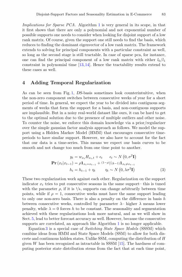
Disjoint-Support Factors and Seasonality Estimation in E-Commerce 83
Implications for Sparse PCA. Algorithm 1 is very general in its scope, in thatit first shows that there are only a polynomial and not exponential number ofpossible supports one needs to consider when looking for disjoint support of a lowrank matrix. Of course, given the support one still needs to find the basis, whichreduces to finding the dominant eigenvector of a low rank matrix. The frameworkextends to solving for principal components with a particular constraint as well,so long as the second stage is still tractable. In case of sparse pca, for instance,one can find the principal component of a low rank matrix with either l0/l1constraint in polynomial time [13,14]. Hence the tractability results extend tothese cases as well.
4 Adding Temporal Regularization
As can be seen from Fig. 1, DS-basis sometimes look counterintuitive, whenthe non-zero component switches between consecutive weeks of year for a shortperiod of time. In general, we expect the year to be divided into contiguous seg-ments of weeks that form the support for a basis, and non-contiguous supportsare implausible. But in a noisy real-world dataset like ours, it can be hard to getto the optimal solution due to the presence of multiple outliers and other noise.To counter the noise, we enforce this domain knowledge via a prior/regularizerover the simple gaussian factor analysis approach as follows. We model the sup-port using a Hidden Markov Model (HMM) that encourages consecutive time-periods to have similar support. However, we also have to account for the factthat our data is a time-series. This means we expect our basis curves to besmooth and not change too much from one time point to another.
yt = wxtHxt,t + εt εt ∼ N
(0, σ2I
)
Pr (xt|xt−1) = ρ1xt=xt−1 + (1−ρ)/(k−1)1xt �=xt−1
ht = ht−1 + ηt ηt ∼ N(0, λσ2I
)(3)
These two regularization work against each other. Regularization on the supportindicator xt tries to put consecutive seasons in the same support– this is tunedwith the parameter ρ, if it is 1/k, supports can change arbitrarily between timepoints, while if ρ = 1, consecutive weeks must have the same support leadingto only one non-zero basis. There is also a penalty on the difference in basis hbetween consecutive weeks, controlled by parameter λ– higher λ means lowerpenalty, while λ = 0 forces h to be constant. The seasonality and segmentationachieved with these regularizations look more natural, and as we will show inSect. 5, lead to better forecast accuracy as well. However, because the consecutivesupports are correlated, an approach like Algorithm 1 is no longer applicable.
Equation 3 is a special case of Switching State Space Models (SSSM) whichcombine ideas from HMM and State Space Models (SSM) to allow for both dis-crete and continuous hidden states. Unlike SSM, computing the distribution of Hgiven W has been recognized as intractable in SSSM [15]. The hardness of com-puting posterior state distribution stems from the fact that at each time point,
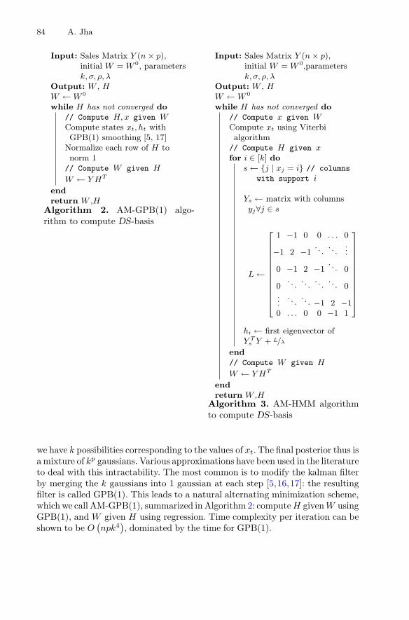
84 A. Jha
Input: Sales Matrix Y (n × p),initial W = W 0, parametersk, σ, ρ, λ
Output: W , HW ← W 0
while H has not converged do// Compute H, x given WCompute states xt, ht withGPB(1) smoothing [5, 17]
Normalize each row of H tonorm 1
// Compute W given H
W ← Y HT
endreturn W ,H
Algorithm 2. AM-GPB(1) algo-rithm to compute DS-basis
Input: Sales Matrix Y (n × p),initial W = W 0,parametersk, σ, ρ, λ
Output: W , HW ← W 0
while H has not converged do// Compute x given WCompute xt using Viterbialgorithm
// Compute H given xfor i ∈ [k] do
s ← {j | xj = i} // columns
with support i
Ys ← matrix with columnsyj∀j ∈ s
L ←
⎡
⎢⎢⎢⎢⎢⎢⎢⎢⎢⎢⎢⎣
1 −1 0 0 . . . 0
−1 2 −1. . .
. . ....
0 −1 2 −1. . . 0
0. . .
. . .. . .
. . . 0...
. . .. . . −1 2 −1
0 . . . 0 0 −1 1
⎤
⎥⎥⎥⎥⎥⎥⎥⎥⎥⎥⎥⎦
hi ← first eigenvector ofY T
s Y + L/λ
end// Compute W given H
W ← Y HT
endreturn W ,H
Algorithm 3. AM-HMM algorithmto compute DS-basis
we have k possibilities corresponding to the values of xt. The final posterior thus isa mixture of kp gaussians. Various approximations have been used in the literatureto deal with this intractability. The most common is to modify the kalman filterby merging the k gaussians into 1 gaussian at each step [5,16,17]: the resultingfilter is called GPB(1). This leads to a natural alternating minimization scheme,which we call AM-GPB(1), summarized in Algorithm 2: compute H given W usingGPB(1), and W given H using regression. Time complexity per iteration can beshown to be O
(npk4
), dominated by the time for GPB(1).

Disjoint-Support Factors and Seasonality Estimation in E-Commerce 85
However, GPB(1)-smoothing is expensive and the execution cost builds upbecause of the repeated calls involved with the alternating minimization involved.We also pursue an alternative way in which we put more emphasis on findingstates x instead. Observe that given support x, we can find basis i as the firsteigenvector of Y (i)T Y (i) + L/λ, where Y (i) is the matrix with columns of supporti from Y , and L is a tridiagonal matrix with 2 on diagonal, except the firstand last, and −1 off-diagonal. Also, once we know H, W is just Y HT . Now, weuse W to find x using the forward backward algorithm for state estimation inHMM. Note that this step completely ignores H, and just finds optimal x for thegiven W . In other words, while GPB(1) smoothing focuses more on estimatingH, this approach puts more emphasis on x. The time complexity per iterationnow is O
(npk + p3
). We call it AM-HMM, summarized in Algorithm 3, and it
also leads to a faster execution time as we will demonstrate empirically.
5 Empirical Evaluation
In this section, we will look at the impact of DS-basis on forecast accuracy ina real-world dataset, and also explore the robustness and performance of thealgorithms proposed in this paper on a synthetic dataset. Our implementation isin C++ and R, and experiments are conducted on a MacBook Pro with 16 GBmemory and 2.5 GHz Intel i7 processor.
5.1 E-Commerce Data
In this section, we use sales data from Walmart E-Commerce. 20 groups of itemsfrom different sections of the catalog are selected, with sizes varying from about2 K to 10 K, for a total of around 50 K items. We should point out that thesegroups were not manually selected; they are actual groups of items assigned toa particular category in the catalogue. In that sense, the items they contain arerepresentative of an e-commerce assortment. We will compare the forecasts fromlocal level model in (1) with k = 3, λμ = λω = 0.1. For forecasts, we choosesix different weeks of year distributed throughout year. For each week, we fore-casted six weeks ahead. Our benchmark for comparison are seasonal factors gen-erated using PCA. To compare how a new forecast f compares to benchmark g, welook at the metric of percentage improvement offered by f over g: |f−s|−|g−s|/|f−s|,where s is the sales. We compute DS-basis for each group using Algorithm 11, andDS-basis(temporal) with temporal regularization is computed using AM-HMM.
Figure 3 shows that there is a stark difference in comparison when it comes toitems with less than a year of history and items with long history, with medianimprovement of 20–30% possible with DS-basis. This is in accordance with theargument made in Sect. 1 that having orthogonal basis is not sufficient whenthe time-series involved are short, since it can be hard to disambiguate between
1 We don’t explore the full search space but use randomization to run within a timebudget.
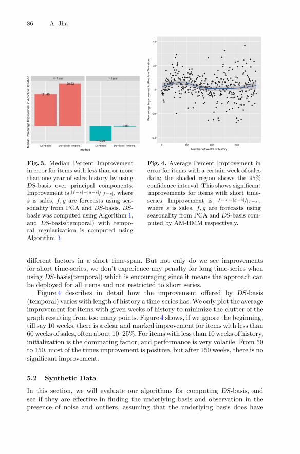
86 A. Jha
Fig. 3. Median Percent Improvementin error for items with less than or morethan one year of sales history by usingDS-basis over principal components.Improvement is |f−s|−|g−s|/|f−s|, wheres is sales, f, g are forecasts using sea-sonality from PCA and DS-basis. DS-basis was computed using Algorithm 1,and DS-basis(temporal) with tempo-ral regularization is computed usingAlgorithm 3
Fig. 4. Average Percent Improvement inerror for items with a certain week of salesdata; the shaded region shows the 95%confidence interval. This shows significantimprovements for items with short time-series. Improvement is |f−s|−|g−s|/|f−s|,where s is sales, f, g are forecasts usingseasonality from PCA and DS-basis com-puted by AM-HMM respectively.
different factors in a short time-span. But not only do we see improvementsfor short time-series, we don’t experience any penalty for long time-series whenusing DS-basis(temporal) which is encouraging since it means the approach canbe deployed for all items and not restricted to short series.
Figure 4 describes in detail how the improvement offered by DS-basis(temporal) varies with length of history a time-series has. We only plot the averageimprovement for items with given weeks of history to minimize the clutter of thegraph resulting from too many points. Figure 4 shows, if we ignore the beginning,till say 10 weeks, there is a clear and marked improvement for items with less than60 weeks of sales, often about 10–25%. For items with less than 10 weeks of history,initialization is the dominating factor, and performance is very volatile. From 50to 150, most of the times improvement is positive, but after 150 weeks, there is nosignificant improvement.
5.2 Synthetic Data
In this section, we will evaluate our algorithms for computing DS-basis, andsee if they are effective in finding the underlying basis and observation in thepresence of noise and outliers, assuming that the underlying basis does have
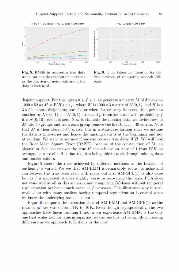
Disjoint-Support Factors and Seasonality Estimation in E-Commerce 87
Fig. 5. RMSE in recovering true datausing various decomposition methodsas the fraction of noisy outliers in thedata is increased.
Fig. 6. Time taken per iteration for thetwo methods of computing smooth DS-basis
disjoint support. For this, given 0 ≤ f ≤ 1, we generate a matrix M of dimension1000×52 as M = WH +ε+μ, where W is 1000×3 matrix of N (0, 1), and H is a3 × 52 smooth disjoint support factor where factors vary from one time-point toanother by N (0, 0.1). ε is N (0, 1) error and μ is outlier noise: with probability fit is N (0, 10), else it is zero. Now to simulate the missing data, we divide rows ofM into 50 groups and from each group remove the first 0, 1, . . . , 49 entries. Notethat M is then about 50% sparse, but in a stair-case fashion since we assumethe data is time-series and hence the missing data is at the beginning and notat random. We want to see now if one can recover true data: WH. We will lookthe Root Mean Square Error (RMSE); because of the construction of M , analgorithm that can recover the true H can achieve an rmse of 1 from WH onaverage, because of ε. But that requires being able to work through missing dataand outlier noise μ.
Figure 5 shows the rmse achieved by different methods as the fraction ofoutliers f is varied. We see that AM-HMM is remarkably robust to noise andcan recover the true basis even with many outliers. AM-GPB(1) is also closebut as f is increased, it does slightly worse in recovering the basis. PCA doesnot work well at all in this scenario, and computing DS-basis without temporalregularization performs much worse as f increases. This illustrates why in real-world data with many outliers having temporal regularization is crucial whenwe know the underlying basis is smooth.
Figure 6 compares the execution time of AM-HMM and AM-GPB(1) as therows of M are varied from 1 K to 10 K. Even though asymptotically, the twoapproaches have linear running time, in our experience AM-HMM is the onlyone that scales well for large groups, and we can see this in the rapidly increasingdifference as we approach 10 K items in the plot.
88 A. Jha
References
1. Makridakis, S., Wheelwright, S.C., Hyndman, R.J.: Forecasting Methods andApplications. Wiley, New Delhi (2008)
2. Fuller, W.A.: Introduction to Statistical Time Series, vol. 428. Wiley, New York(2009)
3. Brockwell, P.J., Davis, R.A.: Time Series: Theory and Methods. Springer,New York (2013)
4. Koren, Y., Bell, R., Volinsky, C.: Matrix factorization techniques for recommendersystems. Computer 42(8), 30–37 (2009)
5. Bar-Shalom, Y., Li, X.-R.: Estimation and Tracking- Principles, Techniques, andSoftware. Artech House Inc., Norwood (1993)
6. Cleveland, R.B., Cleveland, W.S., McRae, J.E., Terpenning, I.: STL: a seasonal-trend decomposition procedure based on loess. J. Official Stat. 6(1), 3–73 (1990)
7. Gelman, A., Hill, J.: Data Analysis Using Regression and Multilevel/HierarchicalModels. Cambridge University Press, New York (2006)
8. Jha, A., Ray, S., Seaman, B., Dhillon, I.S.: Clustering to forecast sparse time-seriesdata. In: 2015 IEEE 31st International Conference on Data Engineering (ICDE),pp. 1388–1399. IEEE (2015)
9. Sun, W., Malioutov, D.: Time series forecasting with shared seasonality patternsusing non-negative matrix factorization. In: NIPS Time Series Workshop (2015)
10. Taylor, J.W., De Menezes, L.M., McSharry, P.E.: A comparison of univariate meth-ods for forecasting electricity demand up to a day ahead. Int. J. Forecast. 22(1),1–16 (2006)
11. Asteris, M., Papailiopoulos, D., Kyrillidis, A., Dimakis, A.G.: Sparse PCA viabipartite matchings. In: Advances in Neural Information Processing Systems, pp.766–774 (2015)
12. Goyal, V., Ravi, R.: An FPTAS for minimizing a class of low-rank quasi-concavefunctions over a convex set. Oper. Res. Lett. 41(2), 191–196 (2013)
13. Asteris, M., Papailiopoulos, D.S., Karystinos, G.N.: The sparse principal compo-nent of a constant-rank matrix. IEEE Trans. Inf. Theor. 60(4), 2281–2290 (2014)
14. Karystinos, G.N.: Optimal algorithms for binary, sparse, and L1-norm principalcomponent analysis. In: Pardalos, P., Rassias, T. (eds.) Mathematics WithoutBoundaries, pp. 339–382. Springer, New York (2014). https://doi.org/10.1007/978-1-4939-1124-0 11
15. Ghahramani, Z., Hinton, G.E.: Variational learning for switching state-space mod-els. Neural Comput. 12(4), 831–864 (2000)
16. Kim, C.-J.: Dynamic linear models with markov-switching. J. Econometrics 60(1–2), 1–22 (1994)
17. Murphy, K.P.: Switching Kalman filters, technical report, Citeseer (1998)
Event Detection and SummarizationUsing Phrase Network
Sara Melvin1, Wenchao Yu1(B), Peng Ju1, Sean Young2, and Wei Wang1(B)
1 Department of Computer Science, UCLA, Los Angeles, [email protected], [email protected]
2 University of California Institute for Prediction Technology,UCLA, Los Angeles, USA
Abstract. Identifying events in real-time data streams such as Twitteris crucial for many occupations to make timely, actionable decisions. It ishowever extremely challenging because of the subtle difference between“events” and trending topics, the definitive rarity of these events, andthe complexity of modern Internet’s text data. Existing approaches oftenutilize topic modeling technique and keywords frequency to detect eventson Twitter, which have three main limitations: (1) supervised and semi-supervised methods run the risk of missing important, breaking newsevents; (2) existing topic/event detection models are base on words,while the correlations among phrases are ignored; (3) many previousmethods identify trending topics as events. To address these limitations,we propose the model, PhraseNet, an algorithm to detect and summa-rize events from tweets. To begin, all topics are defined as a clustering ofhigh-frequency phrases extracted from text. All trending topics are thenidentified based on temporal spikes of the phrase cluster frequencies.PhraseNet thus filters out high-confidence events from other trendingtopics using number of peaks and variance of peak intensity. We evalu-ate PhraseNet on a three month duration of Twitter data and show theboth the efficiency and the effectiveness of our approach.
Keywords: Event detection · Phrase network · Event summarization
1 Introduction
It has been of interest for many years to have an automated tool to alert andsummarize newsworthy events in real-time. Identifying events in real-time iscrucial for many occupations to make timely, actionable decisions. It is shown tobe extremely challenging to identify these events because of the subtle differencebetween “events” and trending topics, the definitive rarity of these events, andthe complexity of modern Internet’s text data. Existing approaches often utilizetopic modeling technique and keywords frequency to detect events on Twitter,which have three main limitations:
c© Springer International Publishing AG 2017Y. Altun et al. (Eds.): ECML PKDD 2017, Part III, LNAI 10536, pp. 89–101, 2017.https://doi.org/10.1007/978-3-319-71273-4_8

90 S. Melvin et al.
1. Supervised and semi-supervised methods run the risk of missing important,breaking news events [3,5,10,12–14]. These methods share one common weak-ness, they rely on the seeding of keywords for their tool or human labelingof tweets to train their models. This approach runs the risk of missing someevents since their model is scoped to identify only events that fall under theirstatic list of keywords.
2. Many previous methods mistakenly identify trending topics as events [8,11],however the description of an “event” is a unique sub-component to all “top-ics”. Figure 1 shows the difference between event distribution (Paris terroristattack) and topic distribution (discussion of social media photos).
3. Existing methods [1,19] summarize their results with a small grouping ofkeywords that do not convey enough information for a user to know in real-time what occurred. These models are also base on unigram words, while thecorrelations among phrases are ignored.
To address the above limitations, we propose PhraseNet, a model for eventdetection using phrase network. Our method begins by extracting the high-frequency phrases from tweets. Each frequent phrase and relationship betweenphrases are then represented in a phrase network. A community detection algo-rithm is applied to the phrase network to identify a grouping of phases which wedefine as event candidates. Finally, the high-confidence events can be identifiedby three criteria extracted from the event candidate distributions over time: (1)number of peaks in distribution, (2) intensity of peaks and (3) variance of thedistribution.
Defining the unique features of an event is key in designing an event detectionmodel. Consider an event such as the Paris terrorist attack on the offices ofCharlie Hebdo. As you can see in Fig. 1, the words to describe the event spikein a collective frequency on the day of the attack with only a couple of peakspost event. In contrast, words used in the discussion of the non-event topic of
20 40 60 80
Timestep (by day)
0
0.2
0.4
0.6
0.8
1
Nor
mal
ized
Fre
quen
cy
Paris Terrorist Attack Event Distribution
20 40 60 80
Timestep (by day)
0
0.2
0.4
0.6
0.8
1
Nor
mal
ized
Fre
quen
cy
Non-event Topic Distribution of Social Media Photos
Fig. 1. A comparison between the distributions of an event and a topic. This figureshows the normalized frequency distribution between a non-event topic discussion ofsocial media photos (right) and the event distribution describing the Paris TerroristAttack (left) at the offices of Charlie Hebdo.

Event Detection and Summarization Using Phrase Network 91
social media photo opinions spike in frequency during several different time stepsthroughout the data. Therefore, the characteristic of an event’s distribution isdefined to have very few peaks because an event description is usually unique;not normally shared by many other events.
In addition, non-event topics are discussed by the masses rises and falls withsimilar frequency throughout time because of the common interest in such topicsstays fairly consistent. However, events are discussed during the occurrence andpost-event to discuss opinions about the event or, if the events are planned,events can discussed prior in anticipation. These event peaks that occur prior-and post-event will be small in frequency compared to the moment the eventoccurs, therefore the standard deviation of an event’s peak intensity will be largerthan a non-event topic because of the varied interest in discussing the event. Asyou can see in Fig. 1, the Paris attack was not planned, there will be no peaksprior to the event occurrence.
Finally, our method, PhraseNet, leverages phrases and graph clustering togroup correlated phrases together and help give more context to the identifiedevent. You will see in Sect. 4.3 how PhraseNet summarizes compared to Twevent.
In summary, our contributions in this paper are:
1. Event detection using phrase network : We proposed the PhraseNet model todetect and summarize events on Twitter stream which includes three steps:(1) building phrase network using high-frequency phrases extracted fromtweets, (2) detecting event candidates using community detection algorithmon phrase network, (3) identifying high-confidence events from candidate setusing criteria such as number of peaks and variance of peak intensity in theevent candidate distributions.
2. Event summarization with phrases: The proposed model summarizes eventswith phrases to give an interested user a short description and time durationof the detected event.
3. Empirical improvements over Twevent : We evaluate the PhraseNet model ona three month duration of Twitter data, and show that PhraseNet outper-forms the baseline Twevent [9] by a large margin, which demonstrates theeffectiveness of our model.
2 Problem Definition
In this section, we formally define a phrase as a sequence of contiguous tokens [6]:
pm = {wd,i, . . . , wd,i+n}, i + n ≤ Nd (1)
where wd,i is a word (a.k.a. token) in the i-th place of the document d; n ≥ 0.The d-th document is a sequence of Nd tokens. A topic consists of a set of phrasesP = {p1, . . . pk} where pm is a phrase and k is the total number of phrases inthe set (m ∈ [1, k]).
A sliding window, T , consists of τ amount of time steps, t. As the sliding win-dow moves along, a sliding window mean, μT , and the sliding window standard

92 S. Melvin et al.
deviation, σT are calculated as follows:
μT =1τ
τ∑
t=1
(k∑
m=1
F(p(t)m )) (2)
σT =1τ
τ∑
t=1
(k∑
m=1
F(p(t)m ) − μT )2 (3)
where τ is the number of time steps within the sliding window and F(p(t)m ) isthe frequency of phrase pm at time step t in the sliding window T .
A trending topic, or an event candidate, is identified by a peak in topic phrasefrequency above a certain standard deviations from the topic’s mean. Therefore,the peak is defined as:
∑km=1(F(p(t)m )) − μT
σT> θ (4)
where θ is user-specified threshold. Therefore, an event is an unique subset oftrending topics, or event candidates, that is formally defined in this method asa phrase cluster with very few peaks (≤ α), a high frequency intensity of a peak(≥ β), and the largest standard deviation in peak height (≥ χ).
3 Approach
3.1 Creating the Phrase Network
As mentioned in Sect. 2, to identify these phrases, the ToPMine algorithm [6]was used to identify the frequent phrases for a certain unit of time (e.g. anhour) t and to partition each tweet into a combination of frequent. ToPMinealgorithm includes two phases: (1) parse all the words into text segments; (2)create a hashmap of phrases and recursively merge if phrases appear frequentlyenough together.
The second phase is a bottom-up process that results in a partition on theoriginal document that, when completed, creates a “bag-of-phrases.” For exam-ple, the following tweet: american sniper wins for putting bradley in that body#oscars2015. Would be partitioned with the following phrases with a minimumsupport of 50: american sniper, bradley.
Now each frequent phrase found is considered a node in a graph. The edgesbetween each frequent phrase reflect the co-occurrence of the phrases in thesame tweet. The weight to the edge, we, is the Jaccard coefficient defined aswe = F(pa∧pb)
F(pa)+F(pb), where the edge connects the phrases pa and pb.
To calculate the most frequent co-occurring phrase pairs efficiently, the FP-Growth algorithm [7] was used. In this research, brute force scanning and tallyingup co-occurrences became a bottleneck in PhraseNet, however, the FP-Growthexhibited the speed necessary to keep PhraseNet a real-time algorithm.

Event Detection and Summarization Using Phrase Network 93
3.2 Phrases Clustering
After the graph is constructed, it is clustered into communities of phrases usingthe Louvain community detection method [2], which maximizes the modularity.The clusters identified by this method are event candidates. Hence, output forthis stage is the set of event candidates Ξ = {P1, . . . ,Pc} where c is number ofevent candidates in all time steps. The details are shown in Algorithm 1.
ALGORITHM 1. Phrase network construction and event candidatedetectionData: Frequent patterns of phrases P = {pi, F(pi)}Result: List of event candidates, Ξ = {P1, . . . , Pc}
1 Graph G=(V,E)2 for pi, F(pi) in P do3 for pa, pb in pi where a �= b do4 if pa �∈ V then5 V = V ∪ pa
6 if pb �∈ V then7 V = V ∪ pb
8 e = (pa, pb)9 e.weight = F(pa ∧ pb)/(F(pa) + F(pb))
10 E = E ∪ e
11 Ξ = LouvainClustering(G)
12 return Ξ
3.3 Merging Event Candidates Across Time Steps
Since events could potentially carry on beyond the set time interval, each eventcandidate Pi is measured against the other event candidates of the next timestep to measure whether the two event candidates should merge. The criteriaused to determine the merge is the similarity score defined by Eq. (5). If the twoevent candidates with the highest score have a score greater than a threshold(we set 0.5 in this paper), then the event candidates will merge.
similarity = max(
∑ps∈(Pi,t∩Pi,t+1)
ws
∑pr∈Pi,t
wr,
∑ps∈(Pi,t∩Pi,t+1)
ws
∑pj∈Pi,t+1
wj
)(5)
For each time interval there is a set of phrase, P at time step t. Each phrase,pm has a weight, wm associated with it that will be normalized by the totalnumber of phrases in the time interval t, denoted as n in the equation below.
wm =F(pm)∑ni=1 F(pi)
(6)

94 S. Melvin et al.
On completion of merging there remains a set of unique event candidatesare maintained through all time steps. The event candidate distribution overtime is created by defining the frequency of the phrase cluster over each timestep. The frequency of a phrase cluster P will be denoted as F(P). Therefore,F(P) =
∑km=1 wm which is the sum of all phrase weights contained in the
phrase cluster that make up P.
3.4 Peak Detection
PhraseNet identifies potential events by first identifying the trending topics.Trending topics are discussions on a subject that becomes, all of a sudden,popular. To define “all of a sudden,” the z-score was used to calculate the phrasecluster frequency, F(P), is θ standard deviations above the sliding window mean,μt. The z-score was used to better identify peaks in a noisy environment. Forexample, a planned event may be discussed in advance thus showing a F(P) >μt, however, these discussions are only small bumps compared to the height ofthe phrase community on the day of the planned event. To clarify the day andthe duration of the event, whether planned or not planned, z-score helps filterthe larger spikes in frequency compared to the small bumps.
Some events last longer than a time step, therefore, the sliding window aver-age is updated as it slides, however a damping coefficient, ωt, is used to weightthe phrase communities’ peak. Therefore, the sliding window average shown inEq. (2) is updated as follows:
μT =1τ
τ∑
t=1
ωt(k∑
m=1
F(p(t)m )) (7)
where ωt is zero for non-peak topic time steps and during peak time intervals ofa topic the coefficient is 0 ≤ ωt ≤ 1 where ωt ∈ R. The exact definition of ωt isa parameter for the user to define.
Finally, to focus on event candidate peaks, all time steps where the phrasecommunity did not show a peak, their phrase community frequency is loweredto zero, however, all peak identified time steps maintain the phrase communityfrequency,
∑km=1 F(p(t)m ). This filtering is shown in Fig. 1.
Lastly, all event candidates are held to a certain threshold of key featuresand then sorted: the least number of peaks (αi > αj where i �= j), the largeststandard deviation of peak heights (βi < βj where i �= j), and the highest peakintensity (χi < χj where i �= j). The last feature (χ) is used to merely sortbetween the most popular phrase groups to aid in identifying the most urgentevents. The first γ of the event candidates are considered events. Each eventthat has a peak on the same day as another event are joined together for a totalsummary of the time step occurrences.
4 Results
It will be shown in this section how accurate and quick PhraseNet identifiesevents in comparison with Twevent.
Event Detection and Summarization Using Phrase Network 95
4.1 Data and Parameters
Data was collected using Twitter’s REST API1 for the time period of January 1,2015 to March 31, 2015. The sliding window for each time step was set for 24 h,from midnight to midnight. The experiment dataset only used English tweetsthus using a total of 2,747,808 tweets. Each tweet was preprocessed to expand allcontractions, all non-English characters were removed, and all stop words wereremoved.
The ToPMine algorithm uses the minimum support of 40 to find all frequentphrases and phrases were given a limit to search no more than 5-gram. In addi-tion, the FP-Growth algorithm used a minimum support of 8. The θ value wasplaced at a 3, which means all event candidate peaks are identified as more than3 standard deviations above the sliding window mean. The dampening coeffi-cient, ωt, weight was defined as 0.1 and the allowed window of time for a truepositive event peak to occur consisted of the true event date ±5 days. Lastly,the event key feature thresholds are the following: α = 10, β = .05, and χ = .5.
4.2 Experiment and Evaluation
Since ground truth was not available for this dataset, ground truth was definedfrom the “On This Day” website2 and by various other reliable news sources.From the “On This Day” website, all events were filtered to only include Englishspeaking country events (i.e. United States, England, Australia, Canada, andNew Zealand) and terrorist attacks. In addition, all national holidays celebratedby the United States, U.K., Australia, Canada, and New Zealand identified inWikipedia were added to the ground truth. Lastly, all sports related events werefound via ESPN, BBC Sport, or NFL websites. Under this definition of groundtruth, there are 102 events in total.
A sampling of true positives found by PhraseNet are listed in the table foundin Table 1. This table exhibits the correlation of sub-events identified by peakswithin the same time step. For example, the Grammy Awards are described byPhaseNet with some of the winners’ names and included the word “Kanye” and“Beyonce” to note the fact that Kanye, again, interrupted a Grammy winner’sspeech to stick up for his friend Beyonce.
Considering the ground truth for identifying and labeling all true positives,false positives, and false negatives, it is impossible to determine every event thatoccurred within the data time frame, therefore this research uses the metricsof precision and recall. To show the trade off between precision and recall, theF1 score is also provided for comparison. Precision is defined as the number ofevent candidates that correlate to known events divided by total number of eventcandidates. Recall is defined as the number of unique events detected dividedby the total number of events possible listed in the ground truth. The finalperformance of PhraseNet is shown in Fig. 2 and detailed further in Table 2. It is
1 https://dev.twitter.com/rest/public.2 http://www.onthisday.com/events/date/2015.
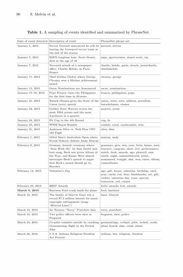
96 S. Melvin et al.
Table 1. A sampling of events identified and summarized by PhraseNet.
Date of event detected Description of event PhraseNet phrase set
January 1, 2015 Steven Gerrard announced he will be
leaving the Liverpool soccer team at
the end of the season
gerrard, steven
January 5, 2015 ESPN longtime host, Scott Stuart,
died at the age of 49
espn, sportscenter, stuart scott, rip
January 7, 2015 Terrorist attack at a newspaper
office, Charlie Hebdo, in Paris,
France
charlie, hebdo, paris, attack, jesuischarlie,
charliehebdo
January 11, 2015 72nd Golden Globes where George
Clooney won a lifetime achievement
award
clooney, george
January 15, 2015 Oscar Nominations are Announced oscar, nominations
January 15–19, 2015 Pope Francis visits the Philippines
for the first time in 20 years
francis, philippines, pope
January 21, 2015 Barack Obama gives the State of the
Union (sotu) speech
union, state, sotu, address, president,
barackobama, obama
January 24, 2015 Golden State Warrior scores the
most NBA points and the most
3-pointers in a quarter
quarter, point
January 24, 2015 FA Cup in the 4th Round cup, fa
January 25, 2015 WWE Royal Rumble rumble, royal, royalrumble, wwe
January 31, 2015 Anderson Silva vs. Nick Diaz UFC
183 Fight
silva, diaz
February 1, 2015 103rd Men’s Australian Open where
Novak Dokovic defeats Andy Murray
murray, andy
February 8, 2015 Grammy Awards ceremony where
“Stay With Me” by Sam Smith won
best song, Beck was given Album of
the Year, and Kanye West almost
interrupts Beck’s speech to argue
that Beck’s award should go to
Beyonce
grammys, give, win, year, brits, kanye, west,
beyonce, congrats, show, live, performance,
watch, beck, awards, ago, pharrell, sam
smith, night, samsmithworld, artist,
nominated, tonight, shit, won, enter, album,
connorfranta
February 14, 2015 Valentine’s Day ago, gift, house, valentine, birthday, card,
year, cards, red, blue, blackhawks, art, gift,
violets, valentine day, roses, special,
tomorrow, red, carpet
February 25, 2015 BRIT Awards brits, awards, brit, awards
March 5, 2015 Harrison Ford crash lands his plane ford, harrison
March 10, 2015 The family of Marvin Gaye win a
record $7.3 million lawsuit for music
copyright infringement (song:
“Blurred Lines”)
lines, blurred
March 12, 2015 Sir Terence “Terry” Pratchett dies terry, pratchett
March 16, 2015 Two police officers were shot in
Ferguson
ferguson, shot, police
March 24, 2015 Co-pilot commits suicide by crashing
Germanwings flight in the French
Alps
germanwings, cockpit, pilot, locked, crash,
plane french, alps, crash, plane
March 26, 2016 U.S.A. Indiana Religious Freedom
Act Protest
indiana, law, religious, freedom
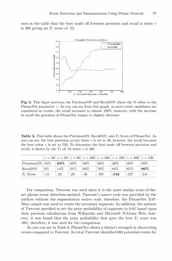
Event Detection and Summarization Using Phrase Network 97
seen in the table that the best trade off between precision and recall is when γis 480 giving an F1 score of .54.
Fig. 2. This figure portrays the Precision@N and Recall@N where the N refers to thePhraseNet parameter γ. As you can see from this graph, as more event candidates areconsidered as events, the recall increases to almost 100%, however, with the increasein recall the precision of PhraseNet begins to slightly decrease.
Table 2. This table shows the Precision@N, Recall@N, and F1 Score of PhraseNet. Asyou can see, the best precision occurs when γ is set to 40, however, the recall becomesthe best when γ is set to 520. To determine the best trade off between precision andrecall, is shown by the F1 of .54 when γ is 480.
γ = 20 γ = 40 γ = 80 γ = 260 γ = 400 γ = 480 γ = 500 γ = 520
Precision@N 55% 63% 48% 36% 36% 40% 39% 39%
Recall@N 8% 14% 21% 60% 78% 84% 85% 86%
F1 Score .14 .23 .29 .46 .491 .542 .537 .541
For comparison, Twevent was used since it is the most similar state-of-the-art phrase event detection method. Twevent’s source code was provided by theauthors without the segmentation source code, therefore, the PhraseNet ToP-Mine output was used to create the necessary segments. In addition, the authorsof Twevent specified to set the prior probability of segments to 0.01 based upontheir previous calculations from Wikipedia and Microsoft N-Gram Web, how-ever, it was found that the prior probability that gave the best F1 score was.001, therefore, it was used for the comparison.
As you can see in Table 3, PhraseNet shows a distinct strength in discoveringevents compared to Twevent. In total Twevent identified 694 potential events for

98 S. Melvin et al.
Table 3. Precision and Recall for the best F1 Score of both PhraseNet and Twevent.
Precision Recall F1 Score
PhraseNet 40% 84% .54
Twevent 2% 15% .04
the three months of data, however, only 22 of those were confirmed true positives.In addition, Twevent identified 11 distinct events out of 102. In comparisonwhen PhraseNet returned 480 potential events, 86 distinct events were correctlyidentified. These results were determined with the same ground truth list andwith the all true positives were identified if found within ±5 days of the trueevent date.
Figure 1 showed an example displaying the key differences between an eventdistribution and a non-event topic distribution. Twevent identified the non-eventtopic of social media photos as an event and the Paris attack was not evenidentified, however, both of these cases were identified correctly by PhraseNet.
One reason for Twevent’s performance is the mistake of identifying a non-event topic as an event. This is due to the mechanism that determines a “bursty”segment. Some words are frequent, however, their popularity in usage tends torise and fall in its frequency throughout time. PhraseNet can find these groups ofphrase segments and recognizes these multiple rises and falls as a characteristicof a non-event topic.
There was one common weakness made by Twevent and PhraseNet. Theyboth mistakenly identified some non-event topics as events because these partic-ular non-event topics showed event-like characteristics. For example, some artistshave an army of users spreading a marketing campaign across social media topre-order their new album. These types of discussions do not continue afterthe initial push from the artist’s publicist, therefore, there shows a single highfrequency peak on the day of the marketing campaign, yet no other frequencythroughout the rest of the data.
4.3 Event Summarization: A Case Study
PhraseNet gives a more holistic picture about an event by leveraging phrases andgraph clustering than other phrase focused event detection methods. For exam-ple, the Super Bowl event detected by PhraseNet consists of the following setof phrases: superbowl, super bowl, pats, watch, year, vote, superbowlxlix, seattle,end, patriotswin, patriots, fans, call, katy perry, music, play, hase, commercial,f**k, s**t, depressing, game, seahawks, win, ago, nfl, chance, team, sb, halftimeshow, win sb, mousetrapspellingbee, video, youtube, kianlawley. This description,correlated, aggregated, and produced by PhraseNet, explains that the SeattleSeahawks and the Patriots played in the NFL Super Bowl XLIL and, from the“patriotswin” hashtag, the Super Bowl was won by the Patriots. In addition,PhraseNet unveils that the Super Bowl half time show starred Katy Perry.
Event Detection and Summarization Using Phrase Network 99
However, Twevent [9] gives a description of the same event with the followingkeywords: rt, superbowl, ve, super bowl, ll, commercial, watch, game, seahawks,time, patriots. This description of the Super Bowl leaves out the half time showdescription and who eventually won the game.
4.4 Scalability and Efficiency
PhraseNet can be implemented in real-time. PhraseNet has a complexity ofO(τn) where τ is the number of intervals of the sliding window (i.e. number ofdocuments) and n is the number of phrases within each sliding window, therefore,it scales to be a suitable algorithm for real-time. Under the experiment settingdescribed in Sect. 4.1, the running time of PhraseNet is 8.12 s per time step wherethe experiment was run on a Macbook Pro 2.2 GHz Intel Core i7 with 16 GB ofmemory. It takes Twevent 45.95 s under the same setting.
5 Related Work
Twitter opens up doors to a faster way to gain information and to connect.People became a form of social “sensors” [16]. Many event detection algorithmshave been proposed, both supervised and unsupervised, based on this platform.
Supervised Methods. Supervised methods focus on a certain set of seed key-words or hashtags which causes the method to miss events that have never beenseen before or other important, unique, and rare events. This limits the ability ofthe system to rapidly evolving with its users and the evolving environment theusers interact and live [3,5,10,12,13]. Thelwall et al. [18] showed evidence thatstrong negative or positive sentiment about a subject would separate out theevents. However, the sentiment was found of a specific set of seeded keywordsand hashtags used for tweet correlation which biases the detections to past dataand recurring events.
Unsupervised Methods. Some event detection papers, such as Twevent, [9],consider trending (aka “bursty”) topics as synonymous to events, however, notall topics are events [8,11,20]. Other methods are more semi-supervised methodssince they need seeded events to learn from to identify events in the midst ofother topics. FRED [14] use training data labeled as “newsworthy” to aid inseeding the model. In addition, GDTM [4] explores a graphical model approachwhich relies on keywords to seed their unsupervised topic modeling. Ritter et al.[15] developed a semi-supervised method which makes use of text annotation,however, in the midst of an informal environment such as Twitter, annotationscould easily be mistaken. HIML [21] and EMBERS [17] methods required analready established taxonomy to find complex events. The taxonomy focuses onlocation information given in the text, which is hardly ever the case for Twitterdata. TopicSketch [19] identifies “bursty topics” in real time where topics aredefined as a word used more frequently at a rate greater than a threshold anddoes so uniquely. Agarwal et al. [1] similarly use keywords that occur together in

100 S. Melvin et al.
the same tweet appearing in a short sliding window (“burstiness” of a keyword)to identify potential events. In addition, this method uses a greedy clique clus-tering method to incrementally find small, dense clusters which limits the finaldescription of the event.
6 Conclusion
PhraseNet has exhibited to be an unsupervised, real-time Twitter event detec-tion algorithm that summarizes events with a grouping of phrases. PhraseNetshowed to have no bias towards certain types of events by being unsupervised,PhraseNet distinguished out non-event topics from events, and gave a shortdescription of the events with a short keyword description. For potential futurework, we want to identify dependencies between events and calculate the prob-ability of influence unsupervised.
Acknowledgement. The work is partially supported by NIH U01HG008488, NIHR01GM115833, NIH U54GM114833, and NSF IIS-1313606. We thank the anonymousreviewers for their careful reading and insightful comments on our manuscript.
References
1. Agarwal, M.K., Ramamritham, K., Bhide, M.: Real time discovery of dense clus-ters in highly dynamic graphs: identifying real world events in highly dynamicenvironments. VLDB 5(10), 980–991 (2012)
2. Blondel, V.D., Guillaume, J.-L., Lambiotte, R., Lefebvre, E.: Fast unfolding of com-munities in large networks. J. Stat. Mech. Theor. Exp. 2008(10), P10008 (2008)
3. Bollen, J., Mao, H., Zeng, X.: Twitter mood predicts the stock market. J. Comput.Sci. 2(1), 1–8 (2011)
4. Chua, F.C.T., Asur, S.: Automatic summarization of events from social media. In:ICWSM (2013)
5. Du, N., Dai, H., Trivedi, R., Upadhyay, U., Gomez-Rodriguez, M., Song, L.: Recur-rent marked temporal point processes: embedding event history to vector. In: KDD,pp. 1555–1564. ACM (2016)
6. El-Kishky, A., Song, Y., Wang, C., Voss, C.R., Han, J.: Scalable topical phrasemining from text corpora. VLDB 8(3), 305–316 (2014)
7. Han, J., Pei, J., Yin, Y.: Mining frequent patterns without candidate generation.In: SIGMOD, vol. 29, pp. 1–12. ACM (2000)
8. Kwak, H., Lee, C., Park, H., Moon, S.: What is Twitter, a social network or a newsmedia? In: WWW, pp. 591–600. ACM (2010)
9. Li, C., Sun, A., Datta, A.: Twevent: segment-based event detection from tweets.In: CIKM, pp. 155–164. ACM (2012)
10. Lin, C.X., Zhao, B., Mei, Q., Han, J.: PET: a statistical model for popular eventstracking in social communities. In: KDD, pp. 929–938. ACM (2010)
11. Mathioudakis, M., Koudas, N.: TwitterMonitor: trend detection over the Twitterstream. In: SIGMOD, pp. 1155–1158. ACM (2010)
12. Popescu, A.-M., Pennacchiotti, M.: Detecting controversial events from Twitter.In: CIKM, pp. 1873–1876. ACM (2010)

Event Detection and Summarization Using Phrase Network 101
13. Popescu, A.-M., Pennacchiotti, M., Paranjpe, D.: Extracting events and eventdescriptions from Twitter. In: WWW, pp. 105–106. ACM (2011)
14. Qin, Y., Zhang, Y., Zhang, M., Zheng, D.: Feature-rich segment-based news eventdetection on Twitter. In: IJCNLP, pp. 302–310 (2013)
15. Ritter, A., Etzioni, O., Clark, S., et al.: Open domain event extraction from Twit-ter. In: KDD, pp. 1104–1112. ACM (2012)
16. Sakaki, T., Okazaki, M., Matsuo, Y.: Earthquake shakes Twitter users: real-timeevent detection by social sensors. In: WWW, pp. 851–860. ACM (2010)
17. Saraf, P., Ramakrishnan, N.: EMBERS AutoGSR: automated coding of civil unrestevents. In: KDD, pp. 599–608. ACM (2016)
18. Thelwall, M., Buckley, K., Paltoglou, G.: Sentiment in Twitter events. J. Assoc.Inf. Sci. Technol. 62(2), 406–418 (2011)
19. Xie, W., Zhu, F., Jiang, J., Lim, E.-P., Wang, K.: TopicSketch: real-time burstytopic detection from Twitter. TKDE 28(8), 2216–2229 (2016)
20. Yu, W., Aggarwal, C.C., Wang, W.: Temporally factorized network modeling forevolutionary network analysis. In: WSDM, pp. 455–464. ACM (2017)
21. Zhao, L., Ye, J., Chen, F., Lu, C.-T., Ramakrishnan, N.: Hierarchical incompletemulti-source feature learning for spatiotemporal event forecasting. In: KDD, pp.2085–2094. ACM (2016)
Generalising Random Forest ParameterOptimisation to Include Stability and Cost
C. H. Bryan Liu1(B), Benjamin Paul Chamberlain2, Duncan A. Little1,and Angelo Cardoso1
1 ASOS.com, London, [email protected]
2 Department of Computing, Imperial College London, London, UK
Abstract. Random forests are among the most popular classificationand regression methods used in industrial applications. To be effective,the parameters of random forests must be carefully tuned. This is usu-ally done by choosing values that minimize the prediction error on aheld out dataset. We argue that error reduction is only one of severalmetrics that must be considered when optimizing random forest para-meters for commercial applications. We propose a novel metric that cap-tures the stability of random forest predictions, which we argue is keyfor scenarios that require successive predictions. We motivate the needfor multi-criteria optimization by showing that in practical applications,simply choosing the parameters that lead to the lowest error can intro-duce unnecessary costs and produce predictions that are not stable acrossindependent runs. To optimize this multi-criteria trade-off, we present anew framework that efficiently finds a principled balance between thesethree considerations using Bayesian optimisation. The pitfalls of optimis-ing forest parameters purely for error reduction are demonstrated usingtwo publicly available real world datasets. We show that our frameworkleads to parameter settings that are markedly different from the valuesdiscovered by error reduction metrics alone.
Keywords: Bayesian optimisation · Parameter tuningRandom forest · Machine learning application · Model stability
1 Introduction
Random forests are ensembles of decision trees that can be used to solve classifi-cation and regression problems. They are very popular for practical applicationsbecause they can be trained in parallel, easily consume heterogeneous data typesand achieve state of the art predictive performance for many tasks [6,14,15].
Forests have a large number of parameters (see [4]) and to be effective theirvalues must be carefully selected [8]. This is normally done by running an opti-misation procedure that selects parameters that minimize a measure of predic-tion error. A large number of error metrics are used depending on the prob-lem specifics. These include prediction accuracy and area under the receiverc© Springer International Publishing AG 2017Y. Altun et al. (Eds.): ECML PKDD 2017, Part III, LNAI 10536, pp. 102–113, 2017.https://doi.org/10.1007/978-3-319-71273-4_9

Generalising Random Forest Parameter Optimisation to Include Stability 103
operating characteristic curve (AUC) for classification, and mean absolute error(MAE) and root mean squared error (RMSE) for regression problems. Para-meters of random forests (and other machine learning methods) are optimizedexclusively to minimize error metrics. We make the case to consider monetarycost in practical scenarios and introduce a novel metric which measures thestability of the model.
Unlike many other machine learning methods (SVMs, linear regression, deci-sion trees), predictions made by random forests are not deterministic. Whilea deterministic training method has no variability when trained on the sametraining set, it exhibits randomness from sampling the training set. We callthe variability in predictions due solely to the training procedure (includingtraining data sampling) the endogenous variability. It has been known formany years that instability plays an important role in evaluating the perfor-mance of machine learning models. The notion of instability for bagging models(like random forests) was originally developed by Breiman [1,2], and extendedexplicitly by Elisseeff et al. [5] to randomised learning algorithms, albeit focusingon generalisation/leave-one-out error (as is common in computational learningtheory) rather than the instability of the predictions themselves.
It is often the case that changes in successive prediction values are moreimportant than the absolute values. Examples include predicting disease risk [9]and changes in customer lifetime value [3]. In these cases we wish to measure achange in the external environment. We call the variability in predictions duesolely to changes in the external environment exogenous variability. Figure 1illustrates prediction changes with and without endogenous changes on top ofexogenous change. Ideally we would like to measure only exogenous change,which is challenging if the endogenous effects are on a similar or larger scale.
Besides stability and error our framework also accounts for the cost of runningthe model. The emergence of computing as a service (Amazon elastic cloud, MSAzure etc.) makes the cost of running machine learning algorithms transparentand, for a given set of resources, proportional to runtime.
It is not possible to find parameter configurations that simultaneously opti-mise cost, stability and error. For example, increasing the number of trees ina random forest will improve the stability of predictions, reduce the error, butincrease the cost (due to longer runtimes). We propose a principled approach tothis problem using a multi-criteria objective function.
We use Bayesian optimisation to search the parameter space of the multi-criteria objective function. Bayesian optimisation was originally developed byKushner [10] and improved by Mockus [12]. It is a non-linear optimisation frame-work that has recently become popular in machine learning as it can find optimalparameter settings faster than competing methods such as random/grid searchor gradient descent [13]. The key idea is to perform a search over possible para-meters that balances exploration (trying new regions of parameter space weknow little about) with exploitation (choosing parts of the parameter space thatare likely to lead to good objectives). This is achieved by placing a prior dis-tribution on the mapping from parameters to the loss. An acquisition function
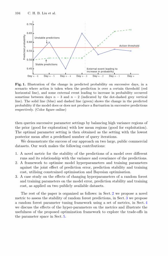
104 C. H. B. Liu et al.
Fig. 1. Illustration of the change in predicted probability on successive days, in ascenario where action is taken when the prediction is over a certain threshold (redhorizontal line), and some external event leading to increase in probability occurredsometime between days n − 3 and n − 2 (indicated by the dot-dashed grey verticalline). The solid line (blue) and dashed line (green) shows the change in the predictedprobability if the model does or does not produce a fluctuation in successive predictionsrespectively. (Color figure online)
then queries successive parameter settings by balancing high variance regions ofthe prior (good for exploration) with low mean regions (good for exploitation).The optimal parameter setting is then obtained as the setting with the lowestposterior mean after a predefined number of query iterations.
We demonstrate the success of our approach on two large, public commercialdatasets. Our work makes the following contributions:
1. A novel metric for the stability of the predictions of a model over differentruns and its relationship with the variance and covariance of the predictions.
2. A framework to optimise model hyperparameters and training parametersagainst the joint effect of prediction error, prediction stability and trainingcost, utilising constrained optimisation and Bayesian optimisation.
3. A case study on the effects of changing hyperparameters of a random forestand training parameters on the model error, prediction stability and trainingcost, as applied on two publicly available datasets.
The rest of the paper is organized as follows: in Sect. 2 we propose a novelmetric to assess the stability of random forest predictions, in Sect. 3 we proposea random forest parameter tuning framework using a set of metrics, in Sect. 4we discuss the effects of the hyper-parameters on the metrics and illustrate theusefulness of the proposed optimization framework to explore the trade-offs inthe parameter space in Sect. 5.

Generalising Random Forest Parameter Optimisation to Include Stability 105
2 Prediction Stability
Here we formalise the notion of random forest stability in terms of repeatedmodel runs using the same parameter settings and dataset (i.e. all variability isendogenous). The expected squared difference between the predictions over tworuns is given by
1N
N∑
i=1
[(y(j)i − y
(k)i
)2]
, (1)
where y(j)i ∈ [0, 1] is the probability from the jth run that the ith data point is of
the positive class in binary classification problems (note this can be extended tomulticlass classification and regression problems). We average over R � 1 runsto give the Mean Squared Prediction Delta (MSPD):
MSPD(f) =2
R(R − 1)
R∑
j=1
j−1∑
k=1
[1N
N∑
i=1
[(y(j)i − y
(k)i
)2] ]
(2)
=2N
N∑
i=1
[1
R − 1
R∑
l=1
(y(l)i − E(y(.)
i ))2
− 1R(R − 1)
R∑
j=1
R∑
k=1
(y(j)i − E(y(.)
i )) (
y(k)i − E(y(.)
i )) ]
= 2Exi[Var(f(xi)) − Cov(fj(xi), fk(xi))], (3)
where Exiis the expectation over all validation data, f is a mapping from a
sample xi to a label yi on a given run, Var(f(xi)) is the variance of the predictionsof a single data point over model runs, and Cov(fj(xi), fk(xi)) is the covarianceof predictions of a single data point over two model runs.1
The covariance, the variance and hence the model instability are closelyrelated to the forest parameter settings, which we discuss in Sect. 4. It is conve-nient to measure stability on the same scale as the forest predictions and so inthe experiments we report the RMSPD =
√MSPD.
3 Parameter Optimisation Framework
In industrial applications, where ultimately machine learning is a tool for profitmaximisation, optimising parameter settings based solely on error metrics isinadequate. Here we develop a generalised loss function that incorporates ourstability metric in addition to prediction error and running costs. We use thisloss with Bayesian optimisation to select parameter values.
1 A full derivation is available at our GitHub repository https://github.com/liuchbryan/generalised forest tuning.

106 C. H. B. Liu et al.
3.1 Metrics
Before composing the loss function we define the three components:
Stability. We incorporate stability (defined in Sect. 2) in to the optimizationframework with the use of the RMSPD.
Error reduction. Many different error metrics are used with random forests.These include F1-score, accuracy, precision, recall and Area Under the receiveroperating characteristics Curve (AUC) and all such metrics fit within our frame-work. In the remainder of the paper we use the AUC because for binary classi-fication, most other metrics require the specification of a threshold probability.As random forests are not inherently calibrated, a threshold of 0.5 may not beappropriate and so using AUC simplifies the exposition [3].
Cost reduction. It is increasingly common for machine learning models to berun on the cloud with computing resources paid for by the hour (e.g. AmazonWeb Services). Due to the exponential growth in data availability, the cost torun a model can be comparable with the financial benefit it produces. We usethe training time (in seconds) as a proxy of the training cost.
3.2 Loss-Function
We choose a loss function that is linear in cost, stability and AUC that allowsthe relative importance of these three considerations to be balanced:
L = β RMSPD(Nt, d, p) + γ Runtime(Nt, d, p) − α AUC(Nt, d, p), (4)
where Nt is the number of trees in the trained random forest, d is the maximumdepth of the trees, and p is the proportion of data points used in training;α, β, γ are weight parameters. We restrict our analysis to three parameters ofthe random forest, but it can be easily extended to include additional parameters(e.g. number of features bootstrapped in each tree).
The weight parameters α, β and γ are specified according to busi-ness/research needs. We recognise the diverse needs across different organisationsand thus refrain from specifying what constitutes a “good” weight parameter set.Nonetheless, a way to obtain the weight parameters is to quantify the gain inAUC, the loss in RMSPD, and the time saved all in monetary units. For example,if calculations reveal 1% gain in AUC equates to £50 potential business profit,1% loss in RMSPD equates to £10 reduction in lost business revenue, and asecond of computation costs £0.01, then α, β and γ can be set as 5,000, 1,000and 0.01 respectively.
3.3 Bayesian Optimisation
The loss function is minimized using Bayesian optimisation. The use of Bayesianoptimisation is motivated by the expensive, black-box nature of the objective
Generalising Random Forest Parameter Optimisation to Include Stability 107
function: each evaluation involves training multiple random forests, a complexprocess with internal workings that are usually masked from users. This rules outgradient ascent methods due to unavailability of derivatives. Exhaustive searchstrategies, such as grid search or random search, have prohibitive runtimes dueto the large random forest parameter space.
A high-level overview on Bayesian Optimisation is provided in Sect. 1. Manydifferent prior functions can be chosen and we use the Student-t process imple-mented in pybo [7,11].
4 Parameter Sensitivity
Here we describe three important random forest parameters and evaluate thesensitivity of our loss function to them.
4.1 Sampling Training Data
Sampling of training data – drawing a random sample from the pool of availabletraining data for model training – is commonly employed to keep the training costlow. A reduction in the size of training data leads to shorter training times andthus reduces costs. However, reducing the amount of training data reduces thegeneralisability of the model as the estimator sees less training examples, leadingto a reduction in AUC. Decreasing the training sample size also decreases thestability of the prediction. This can be understood by considering the form of thestability measure of f , the RMSPD (Eq. 2). The second term in this equation isthe expected covariance of the predictions over multiple training runs. Increasingthe size of the random sample drawn as training data increases the probabilitythat the same input datum will be selected for multiple training runs and thusthe covariance of the predictions increases. An increase in covariance leads to areduction in the RMSPD (see Eq. 3).
4.2 Number of Trees in a Random Forest
Increasing the number of trees in a random forest will decrease the RMSPD (andhence improve stability) due to the Central Limit Theorem (CLT). Consider atree in a random forest with training data bootstrapped. Its prediction can beseen as a random sample from a distribution with finite mean and variance σ2.2
By averaging the trees’ predictions, the random forest is computing the samplemean of the distribution. By the CLT, the sample mean will converge to aGaussian distribution with variance σ2
Nt, where Nt is the number of trees in the
random forest.
2 This could be any distribution as long as its first two moments are finite, which isusually the case in practice as predictions are normally bounded.

108 C. H. B. Liu et al.
To link the variance to the MSPD, recall from Eq. 2 that MSPD capturesthe interaction between the variance of the model and covariance of predictionsbetween different runs:
MSPD(f) = 2Exi[Var(f(xi)) − Cov(fj(xi), fk(xi))].
The covariance is bounded below by the negative square root of the varianceof its two elements, which is in turn bounded below by the negative square rootof the larger variance squared:
Cov(fj(xi), fk(xi)) ≥ −√
Var(fj(xi))Var(fk(xi))
≥ −√
(max{Var(fj(xi)),Var(fk(xi))})2. (5)
Given fj and fk have the same variance as f (being the models with the sametraining proportion across different runs), the inequality 5 can be simplified as:
Cov(fj(xi), fk(xi)) ≥ −√
(max{Var(f(xi)),Var(f(xi))})2 = −Var(f(xi)). (6)
MSPD is then bounded above by a multiple of the expected variance of f :
MSPD(f) ≤ 2Exi[Var(f(xi)) − (−Var(f(xi)))] = 4Exi
[Var(f(xi))], (7)
which decreases as Nt increases, leading to a lower RMSPD estimate.While increasing the number of trees in a random forest reduces error and
improves stability in predictions, it increases the training time and hence mone-tary cost. In general, the runtime complexity for training a random forest growslinearly with the number of trees in the forest.
4.3 Maximum Depth of a Tree
The maximum tree depth controls the complexity of each decision tree and thecomputational cost (running time) increases exponentially with tree depth. Theoptimal depth for error reduction depends on the other forest paramaters and thedata. Too much depth causes overfitting. Additionally, as the depth increases theprediction stability will decrease as each model tends towards memorizing thetraining data. The highest stability will be attained using shallow trees, howeverif the forest is too shallow the model will underfit resulting in low AUC.
5 Experiments
We evaluate our methodology by performing experiments on two public datasets:(1) the Orange small dataset from the 2009 KDD Cup and (2) the Criteo dis-play advertising challenge Kaggle competition from 2014. Both datasets have amixture of numerical and categorical features and binary target labels (Orange:190 numerical, 40 categorical, Criteo: 12 numerical, 25 categorical).
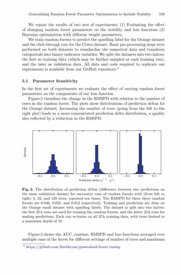
Generalising Random Forest Parameter Optimisation to Include Stability 109
We report the results of two sets of experiments: (1) Evaluating the effectof changing random forest parameters on the stability and loss functions (2)Bayesian optimisation with different weight parameters.
We train random forests to predict the upselling label for the Orange datasetand the click-through rate for the Criteo dataset. Basic pre-processing steps wereperformed on both datasets to standardise the numerical data and transformcategoricals into binary indicator variables. We split the datasets into two halves:the first as training data (which may be further sampled at each training run),and the later as validation data. All data and code required to replicate ourexperiments is available from our GitHub repository.3
5.1 Parameter Sensitivity
In the first set of experiments we evaluate the effect of varying random forestparameters on the components of our loss function.
Figure 2 visualises the change in the RMSPD with relation to the number oftrees in the random forest. The plots show distributions of prediction deltas forthe Orange dataset. Increasing the number of trees (going from the left to theright plot) leads to a more concentrated prediction delta distribution, a qualityalso reflected by a reduction in the RMSPD.
Fig. 2. The distribution of prediction deltas (difference between two predictions onthe same validation datum) for successive runs of random forests with (from left toright) 8, 32, and 128 trees, repeated ten times. The RMSPD for these three randomforests are 0.046, 0.025, and 0.012 respectively. Training and prediction are done onthe Orange small dataset with upselling labels. The dataset is split into two halves:the first 25 k rows are used for training the random forests, and the latter 25 k rows formaking predictions. Each run re-trains on all 25 k training data, with trees limited toa maximum depth of 10.
Figure 3 shows the AUC, runtime, RMSPD and loss functions averaged overmultiple runs of the forest for different settings of number of trees and maximum3 https://github.com/liuchbryan/generalised forest tuning.
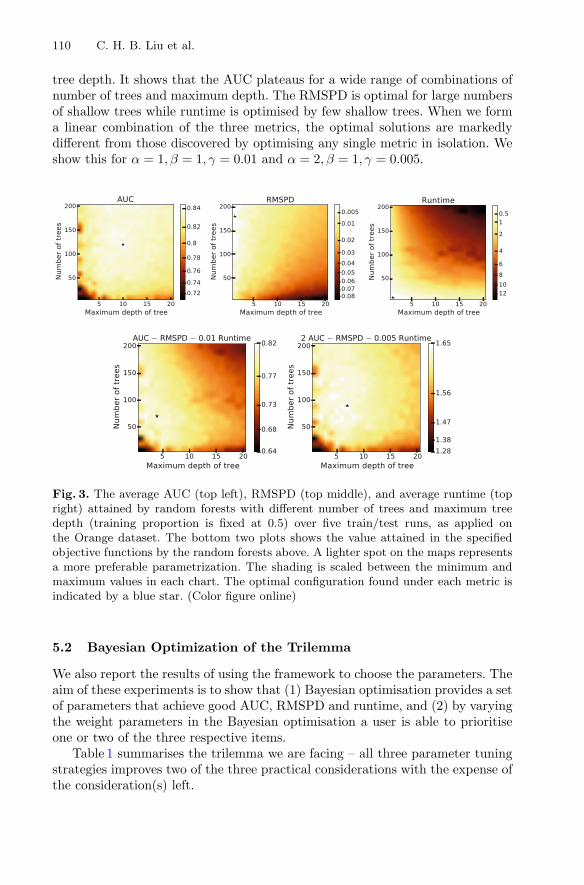
110 C. H. B. Liu et al.
tree depth. It shows that the AUC plateaus for a wide range of combinations ofnumber of trees and maximum depth. The RMSPD is optimal for large numbersof shallow trees while runtime is optimised by few shallow trees. When we forma linear combination of the three metrics, the optimal solutions are markedlydifferent from those discovered by optimising any single metric in isolation. Weshow this for α = 1, β = 1, γ = 0.01 and α = 2, β = 1, γ = 0.005.
Fig. 3. The average AUC (top left), RMSPD (top middle), and average runtime (topright) attained by random forests with different number of trees and maximum treedepth (training proportion is fixed at 0.5) over five train/test runs, as applied onthe Orange dataset. The bottom two plots shows the value attained in the specifiedobjective functions by the random forests above. A lighter spot on the maps representsa more preferable parametrization. The shading is scaled between the minimum andmaximum values in each chart. The optimal configuration found under each metric isindicated by a blue star. (Color figure online)
5.2 Bayesian Optimization of the Trilemma
We also report the results of using the framework to choose the parameters. Theaim of these experiments is to show that (1) Bayesian optimisation provides a setof parameters that achieve good AUC, RMSPD and runtime, and (2) by varyingthe weight parameters in the Bayesian optimisation a user is able to prioritiseone or two of the three respective items.
Table 1 summarises the trilemma we are facing – all three parameter tuningstrategies improves two of the three practical considerations with the expense ofthe consideration(s) left.

Generalising Random Forest Parameter Optimisation to Include Stability 111
Table 1. Effect of the common hyperparameter tuning strategies on the three practicalconsiderations. Plus sign(s) means a positive effect to the measure (and hence morepreferred), and minus sign(s) means a negative effect to the measure (and hence notpreferred). The more plus/minus sign within the entry, the more prominent the effectof the corresponding strategy.
Hyperparameter tuning strategy AUC gain RMSPD reduction Cost savings
Increase training proportion + + –
Increase number of trees + + – –
Reduce maximum depth of trees – + ++
The results of our experiments on Bayesian optimisation of the trilemma areshown in Tables 2 and 3. The first row in both tables shows the results for avanilla random forest with no optimisation of the hyper-parameters discussedin the previous section: 10 trees, no limit on the maximum depth of the tree,and using the entire training data set (no sampling). The Bayesian optimisationfor each set of weight parameters was run for 20 iterations, with the RMSPDcalculated over three training runs in each iteration.
The first observation from both sets of results is that Bayesian optimisation issuitable for providing a user with a framework that can simultaneously improveAUC, RMSPD and runtime as compared to the baseline. Secondly, it is clearthat by varying the weight parameters, Bayesian optimisation is also capable ofprioritising specifically AUC, RMSPD or runtime. Take for example the thirdand fourth rows of Table 2; setting β = 5 we see a significant reduction in theRMSPD in comparison to the second row where β = 1. Similarly, comparing thefourth row to the second row, increasing α from 1 to 5 gives a 1% increase in AUC.In the final row we see that optimising for a short runtime keeps the RMSPDlow in comparison to the non-optimal results on the first row and sacrifices theAUC instead.
Table 2. Results of Bayesian optimisation for the Orange dataset at various settingsof α, β and γ, the weight parameters for the AUC, RMSPD and runtime respectively.The Bayesian optimiser has the ability to tune three random forest hyper-parameters:the number of trees, N∗
t , the maximum tree depth, d∗, and size of the training sample,p∗. Key results are emboldened and discussed further in the text.
α β γ N∗t d∗ p∗ AUC RMSPD Runtime
No optimisation: 0.760 0.112 1.572
1 1 0.01 166 6 0.100 0.829 0.011 1.142
1 5 0.01 174 1 0.538 0.829 0.002 1.452
5 1 0.01 144 12 0.583 0.839 0.013 5.292
1 1 0.05 158 4 0.100 0.8315 0.0082 1.029

112 C. H. B. Liu et al.
For the Criteo dataset (Table 3) we see on the second and third row thatagain increasing the β parameter leads to a large reduction in the RMSPD. Forthis dataset the Bayesian optimiser is more reluctant to use a larger numberof estimators to increase AUC because the Criteo dataset is significantly larger(around 100 times) than the Orange dataset and so using more trees increasesthe runtime more severely. To force the optimiser to use more estimators wereduce the priority of the runtime by a factor of ten as can be seen in the finaltwo rows. We see in the final row that doubling the importance of the AUC (α)leads to a significant increase in AUC (4.5%) when compared to the non-optimalresults.
Table 3. Results of Bayesian optimisation for the Criteo dataset. The table shows theresults of the Bayesian optimisation by varying α, β and γ which control the importanceof the AUC, RMSPD and runtime respectively. The Bayesian optimiser has the abilityto tune three hyper-parameters of the random forest: the number of trees, N∗
t , themaximum depth of the tree, d∗, and size of the training sample, p∗. Key results areemboldened and discussed further in the text.
α β γ N∗t d∗ p∗ AUC RMSPD Runtime
No optimisation: 0.685 0.1814 56.196
1 1 0.01 6 8 0.1 0.7076 0.04673 1.897
1 5 0.01 63 3 0.1 0.6936 0.01081 4.495
1 1 0.05 5 5 0.1 0.688 0.045 1.136
2 1 0.05 9 9 0.1 0.7145 0.03843 2.551
1 1 0.001 120 2 0.1 0.6897 0.007481 7.153
2 1 0.001 66 15 0.1 0.7300 0.02059 11.633
6 Conclusion
We proposed a novel metric to capture the stability of random forest predic-tions, which is key for applications where random forest models are continuouslyupdated. We show how this metric, calculated on a sample, is related to thevariance and covariance of the predictions over different runs. While we focusedon random forests in this text, the proposed stability metric is generic and canbe applied to other non-deterministic models (e.g. gradient boosted trees, deepneural networks) as well as deterministic training methods when training is donewith a subset of the available data.
We also propose a framework for multi-criteria optimisation, using the pro-posed metric in addition to metrics measuring error and cost. We validate thisapproach using two public datasets and show how optimising a model solely forerror can lead to poorly specified parameters.

Generalising Random Forest Parameter Optimisation to Include Stability 113
References
1. Breiman, L.: Bagging predictors. Mach. Learn. 24(2), 123–140 (1996)2. Breiman, L.: Heuristics of instability in model selection. Ann. Stat. 24(6), 2350–
2383 (1996)3. Chamberlain, B.P., Cardoso, A., Liu, C.H.B., Pagliari, R., Deisenroth, M.P.: Cus-
tomer lifetime value prediction using embeddings. In: Proceedings of the 23rd ACMSIGKDD International Conference on Knowledge Discovery and Data Mining, pp.1753–1762 (2017)
4. Criminisi, A.: Decision forests: a unified framework for classification, regres-sion, density estimation, manifold learning and semi-supervised learning. Found.Trends R© Comput. Graph. Vis. 7(2–3), 81–227 (2012)
5. Elisseeff, A., Evgeniou, T., Pontil, M.: Stability of randomized learning algorithms.J. Mach. Learn. Res. 6(1), 55–79 (2005)
6. Fernandez-Delgado, M., Cernadas, E., Barro, S., Amorim, D., Amorim Fernandez-Delgado, D.: Do we need hundreds of classifiers to solve real world classificationproblems? J. Mach. Learn. Res. 15, 3133–3181 (2014)
7. Hoffman, M.W., Shahriari, R.: Modular mechanisms for Bayesian optimization. In:NIPS Workshop on Bayesian Optimization (2014)
8. Huang, B.F.F., Boutros, P.C.: The parameter sensitivity of random forests. BMCBioinform. 17(1), 331 (2016)
9. Khalilia, M., Chakraborty, S., Popescu, M.: Predicting disease risks from highlyimbalanced data using random forest. BMC Med. Inf. Dec. Making 11(1), 51 (2011)
10. Kushner, H.J.: A new method of locating the maximum point of an arbitrarymultipeak curve in the presence of noise. J. Basic Eng. 86(1), 97–106 (1964)
11. Martinez-Cantin, R.: BayesOpt: a bayesian optimization library for nonlinear opti-mization, experimental design and bandits. J. Mach. Learn. Res. 15, 3735–3739(2014)
12. Mockus, J.: On bayesian methods for seeking the extremum. In: Marchuk, G.I. (ed.)Optimization Techniques 1974. LNCS, vol. 27, pp. 400–404. Springer, Heidelberg(1975). https://doi.org/10.1007/3-540-07165-2 55
13. Snoek, J., Larochelle, H., Adams, R.: Practical bayesian optimization of machinelearning algorithms. In: Advances in Neural Information Processing Systems, pp.2951–2959 (2012)
14. Tamaddoni, A., Stakhovych, S., Ewing, M.: Comparing churn prediction techniquesand assessing their performance: a contingent perspective. J. Serv. Res. 19(2), 123–141 (2016)
15. Vanderveld, A., Pandey, A., Han, A., Parekh, R.: An engagement-based customerlifetime value system for e-commerce. In: Proceedings of the 22nd ACM SIGKDDInternational Conference on Knowledge Discovery and Data Mining, pp. 293–302(2016)

Have It Both Ways—From A/B Testing to A&BTesting with Exceptional Model Mining
Wouter Duivesteijn1(B), Tara Farzami2, Thijs Putman2, Evertjan Peer1,Hilde J. P. Weerts1, Jasper N. Adegeest1, Gerson Foks1,
and Mykola Pechenizkiy1
1 Technische Universiteit Eindhoven, Eindhoven, the Netherlands{w.duivesteijn,m.pechenizkiy}@tue.nl,
{e.peer,h.j.p.weerts,j.n.adegeest,g.foks}@student.tue.nl2 StudyPortals B.V., Eindhoven, the Netherlands
{tara,thijs}@studyportals.com
Abstract. In traditional A/B testing, we have two variants of the sameproduct, a pool of test subjects, and a measure of success. In a random-ized experiment, each test subject is presented with one of the two vari-ants, and the measure of success is aggregated per variant. The variantof the product associated with the most success is retained, while theother variant is discarded. This, however, presumes that the companyproducing the products only has enough capacity to maintain one of thetwo product variants. If more capacity is available, then advanced datascience techniques can extract more profit for the company from the A/Btesting results. Exceptional Model Mining is one such advanced data sci-ence technique, which specializes in identifying subgroups that behavedifferently from the overall population. Using the association model classfor EMM, we can find subpopulations that prefer variant A where thegeneral population prefers variant B, and vice versa. This data sciencetechnique is applied on data from StudyPortals, a global study choiceplatform that ran an A/B test on the design of aspects of their website.
Keywords: A/B testing · Exceptional Model Mining · AssociationOnline controlled experiments · E-commerce · Website optimization
1 Introduction
A/B testing [20] is a form of statistical hypothesis testing involving two ver-sions of a product, A and B. Typically, A is the control version of a productand B represents a new variation version, considered to replace A if it proves tobe more successful. An A/B test requires two further elements: a pool of testsubjects, and a measure of success. Each test subject in the pool is presentedwith a randomized choice between A and B. The degree to which this productversion is successful with this test subject is measured. Having collected resultsover the full pool of test subjects, the success degree is aggregated per ver-sion. Subsequently, a decision is made whether the new variation version B is ac© Springer International Publishing AG 2017Y. Altun et al. (Eds.): ECML PKDD 2017, Part III, LNAI 10536, pp. 114–126, 2017.https://doi.org/10.1007/978-3-319-71273-4_10

Have It Both Ways—From A/B Testing to A&B Testing 115
(substantial) improvement over the control version A. For making this decision,a vast statistical toolbox is available [6,7].
Since the rise of the internet, A/B tests have become ubiquitous. It is asimple, cheap, and reliable manner to assess the efficacy of the redesign of a webpage. Running two versions of a web page side by side is not too intrusive toyour online business, and standard web analytics suites will tell you all you needto know on which of the versions deliver the desired results. In fact, throughproper web analytics tools, we can obtain substantially more information on thefactors that influence the success of versions A and B.
Having performed an A/B test, the standard operating procedure is the fol-lowing. An assessment is made whether the new variation version B performs(substantially) better than the current control version A. From that assessment,a hard, binary decision is made: either version A or version B is the winner. Theloser is discarded, and the winner becomes the standard version of the web pagethat is rolled out and presented to all visitors from this moment onwards. Thereis beauty in the simplicity, and this ‘exclusive or’ procedure inspires the slash inthe name of the A/B test.
For large companies, making such a coarse decision leaves potential unused.If you own a high-traffic website, then even a small increase in click-throughrate gets multiplied by a large volume of visitors, which results in a vast increasein income. It makes sense to use the traditional conclusion of an A/B test todetermine the default page that should be displayed to a visitor of which weknow nothing. But it is not uncommon to have some meta-information on thevisitors to your website: which language setting does their browser have, whichOS do they use, in which country are they located, etcetera. If we can identifysubpopulations of the dataset at hand, defined in terms of such metadata, forwhich the A/B test reaches the opposite conclusion from the general popula-tion, then we can generate more revenue with a more sophisticated strategy: wemaintain both versions of the web page, and present a visitor with either A or Bdepending on whether they belong to specific subgroups. Rather than choosingeither A or B, we can instead choose to have it both ways: this paper turns theA/B test into an A&B test.
2 Related Work
First, we provide a brief summary on the current state of the art in mining ofA/B testing results. Thus we explain how our problem formulation is differentfrom existing body of work. Then we overview relevant research in the areas oflocal pattern mining and exceptional model mining that motivate our approachfor the chosen problem formulation.
2.1 Utility of A/B Testing
In a marketing context, A/B testing has been studied extensively [20]. Analysisof the results from an A/B test has made it to the Encyclopedia of Machine
116 W. Duivesteijn et al.
Learning and Data Mining [6], and an extensive survey on experiment designchoices and results analysis is available [7]. This last paper encompasses a discus-sion of accompanying A/B tests with A/A tests to establish a proper baseline,extending the test to the multivariate case (more than two product versions),result confidence intervals, randomization methods to divide the test subjectsfairly over the versions, sample size effects, overlapping experiments, and theeffect of bots on the process. Regardless of the setting of all of these facets, thegoal of A/B testing always remains to make a crisp decision at the end, selectingeither A or B and discarding the alternative(-s).
If the main business goal is to increase the average performance with respectto e.g. a click through rate (CTR) rather than really find our whether A or Bis statistically significantly better, then the Contextual Multi-Armed Bandits(cMAB) is the commonly considered alternative optimization approach to A/Btesting. cMABs help to address an exploration-exploitation trade-off: using, i.e.exploring effectiveness, of A and B provides feedback about its effectiveness(exploration), but collecting that feedback on both A and B is an opportunitycost of exploitation, i.e. using one of the variants we already know is effective. Tobalance exploration with exploitation lots of policy learning bandit algorithmswere considered, particularly in web analytics, e.g. [22,23].
In data mining for user modeling and convergence prediction two relatedproblem formulations have been studied – predictive user modeling with action-able attributes [26] and uplift prediction [18]. While in traditional predictivemodeling, the goal is to learn a model for predicting accurately the class labelfor unseen instances, in targeting applications, a decision maker is interestednot only to generate accurate predictions, but to maximize the probability ofthe desired outcome, e.g. user clicking. Assuming that possibly neither of mar-keting actions A and B is always best, the problem can be formulated as learningto choose the best marketing action at instance level (rather than globally).
The paper that you are currently reading does not have a mission to promoteeither A/B testing or cMABs or uplift prediction; we merely observe that A/Btests are performed anyway, and strive to help companies performing such teststo learn more actionable insight from their data that would allow to domainexperts to decide whether to stay with A, or switch to B or use both A and B,each for a particular context or customer segment.
2.2 Local Pattern Mining
The subfield of Data Mining with which this paper is concerned is Local Pat-tern Mining [4,17]: describing only part of the dataset at hand, while disregard-ing the coherence of the reminder. The Local Pattern Mining subtask that isparticularly relevant here, is Theory Mining [15], where subsets of the datasetare sought that are interesting in some sense. Typically, not just any sub-set is sought. Instead, the focus is on subsets that are easy to interpret. Acanonical choice to enforce that is to restrict the search to subsets that canbe described as a conjunction of a few conditions on single attributes of thedataset. Hence, if the dataset concerns people, we would find subsets of the form

Have It Both Ways—From A/B Testing to A&B Testing 117
“Age ≥ 30 ∧ Smokes = yes ⇒ (interesting)”. Such subsets are referred to assubgroups. Limiting the search to subgroups ensures that the results can be inter-preted in terms of the domain of the dataset at hand; the resulting subgroupsrepresent pieces of information on which a domain expert can act.
Many choices can be made to define ‘interesting’. One such choice is tomake this a supervised concept: we set apart one attribute of the dataset asthe target, and seek subsets that feature an unusual distribution of that target.This is known as Subgroup Discovery (SD) [9,11,25]. In the running exam-ple of a dataset concerning people, if the target would be whether the per-son develops lung cancer or not, SD would find results such as “Smokes =yes ⇒ Lung cancer = yes”. This of course does not mean that all smokersfall in the ‘yes’ category; it merely implies a skew in the target distribution.
2.3 Exceptional Model Mining
Exceptional Model Mining (EMM) can be seen as a generalized form of SD.Instead of singling out one attribute of the data as the target, in EMM onetypically selects several target attributes. The exceptionality of a subgroup isno longer evaluated in terms of an unusual distribution of the single target, butinstead in terms of an unusual interaction between the multiple targets. Thisinteraction is captured by some kind of modeling, which inspired the name ofEMM. Exceptional Model Mining was first introduced in 2008 [13]. An extensiveoverview of the model classes (types of interaction) that have been investigatedcan be found in [3]; as examples, one can think of an unusual correlation betweentwo targets [13], an unusual slope of a regression vector on any number of targets[2], or unusual preference relations [19].
Algorithms for EMM include a form of beam search [3] that works for allmodel classes, a fast sampling-based algorithm for a few dedicated model classes[16], an FP-Growth-inspired tree-based exhaustive algorithm that works foralmost all model classes [14], a tree-constrained gradient ascent algorithm forlinear models using sofy subgroup membership [10], and a compression-basedmethod that improves the resulting models at the cost of interpretability [12].
3 The StudyPortals A/B Test Setting
Since the Bologna process contributed to harmonizing higher-education qualifi-cations throughout Europe, locating (part of) one’s study programme in anothercountry than one’s own has become streamlined. This offers opportunities forstudents to acquire international experience while still studying, which is some-thing from which both the students and the higher education institutions canbenefit. The harmonization of how higher education is structured enables a faircomparison of programmes across country boundaries.
Such a comparison being possible does not necessarily imply that it is alsoeasy. In 2007, three (former) students identified that there was a hole in the infor-mation market, and they filled that hole with a hobby project that eventuallyresulted in StudyPortals [21].

118 W. Duivesteijn et al.
3.1 StudyPortals
In 2007, two alumni from the Technische Universiteit Eindhoven and one fromthe Kungliga Tekniska Hogskolan created MastersPortal: a central database forEuropean Master’s programmes. The goal was to become the primary destinationfor students wanting to study in Europe. In April 2008, the website presented2 700 studies at 200 universities from 30 countries, and attracted 80 000 visitsper month. Since then, the scope of the website has expanded. The subjectranges beyond Master’s programmes, also encompassing Bachelor’s and PhDprogrammes, short courses, scholarships, distance learning, language learning,and preparation courses. The website is no longer restricted to Europe, butexpanded globally. In September 2016, MastersPortal presented 56 000 studiesat 2 000 universities from 100 countries, and attracted 1.4 million unique sessionsper month. The overarching company StudyPortals logged 14.5 million uniquevisitors in the first nine months of 2016, with 7 page views per second during thebusiest hour of the year. This growth allows the company to employ 150 teammembers in five offices on three continents.
StudyPortals generates revenue from the visitors to their websites throughthe universities, who pay for activity on the pages presenting their programmes.A study programme’s web page generates revenue in three streams: (1) Cost PerMille (thousand page views); (2) Cost Per Lead; (3) Cost Per Click. The firstrevenue stream depends on the attractiveness of links towards the programme’sweb page. The second revenue stream depends on whether the person viewingthe programme’s web page fill their personal information in the university leadform. The design of a programme’s web page has a low impact on these tworevenue streams. The third revenue stream is the one that StudyPortals caninfluence directly through appropriate web page design.
3.2 The Third Revenue Stream and the A/B Test
Figure 1 displays the mobile version of a university’s web page on the Master-sPortal website. The orange button at the bottom left of the page links throughto the website of the university itself. When a user clicks on that button, Study-Portals receives revenue in the Cost Per Click revenue stream. With the volumeof web traffic StudyPortals experiences, a small increase in the click-through raterepresents a substantial increase in income.
The advance of smartphones and tablets has vastly increased the impor-tance of the mobile version of websites. These versions come with their own UIrequirements and quirks. Figure 1a displays the page design that was in use inSeptember 2016; having an orange rectangle that is clickable is one of those UIdesign elements that is typical of mobile websites as opposed to desktop versions.However, the website visitors, being human beings, are creatures of habit. Theymight prefer clickable elements of websites to resemble traditional buttons, asthey remember from their desktop dwelling times. To test this hypothesis, Study-Portals designed an alternative version of their mobile website (cf. Fig. 1b). Thesevariants become the subject of our A/B test: the rectangular version is the con-trol version A, and the more buttony version is the variation B.
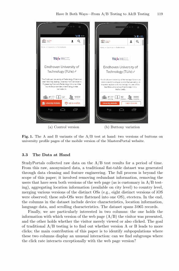
Have It Both Ways—From A/B Testing to A&B Testing 119
(a) Control version (b) Buttony variation
Fig. 1. The A and B variants of the A/B test at hand: two versions of buttons onuniversity profile pages of the mobile version of the MastersPortal website.
3.3 The Data at Hand
StudyPortals collected raw data on the A/B test results for a period of time.From this raw, anonymized data, a traditional flat-table dataset was generatedthrough data cleaning and feature engineering. The full process is beyond thescope of this paper; it involved removing redundant information, removing theusers that have seen both versions of the web page (as is customary in A/B test-ing), aggregating location information (available on city level) to country level,merging various versions of the distinct OSs (e.g., eight distinct versions of iOSwere observed; these sub-OSs were flattened into one OS), etcetera. In the end,the columns in the dataset include device characteristics, location information,language data, and scrolling characteristics. The dataset spans 3 065 records.
Finally, we are particularly interested in two columns: the one holds theinformation with which version of the web page (A/B) the visitor was presented,and the other holds whether the visitor merely viewed or also clicked. The goalof traditional A/B testing is to find out whether version A or B leads to moreclicks; the main contribution of this paper is to identify subpopulations wherethese two columns display an unusual interaction: can we find subgroups wherethe click rate interacts exceptionally with the web page version?

120 W. Duivesteijn et al.
4 Data Science to Be Applied
Finding subsets of the dataset at hand where several columns of special interestinteract in an unusual manner is the core task of Exceptional Model Mining(EMM). This interaction can be gauged in many ways. This section discussesthe EMM framework and its specific instantiation for the problem at hand.
4.1 The Exceptional Model Mining Framework
EMM [3,13] assumes a flat-table dataset Ω, which is a bag of N records of theform r = {a1, . . . , ak, t1, . . . , tm}. We call the attributes a1, . . . , ak the descriptorsof the dataset. These are the attributes in terms of which subgroups will bedefined ; the ones on the left-hand side of the ⇒ sign in the examples of Sect. 2.2.The other attributes, t1, . . . , tm, are the targets of the dataset. These are theattributes in terms of which subgroups will be evaluated ; the most exceptionaltarget interaction indicates the most interesting subgroup.
Subgroups are defined in terms of conditions on descriptors. These induce asubset of the dataset: all records satisfying the conditions. For notational pur-poses, we identify a subgroup with that subset, so that we write S ⊆ Ω, anddenote |S| for the number of records in a subgroup. We also denote SC for thecomplement of subgroup S in dataset Ω, i.e.: SC = Ω\S.
To instantiate the EMM framework, we need to define two things: a modelclass, and a quality measure for that model class. The model class specifies whattype of interaction we are interested in. This can sometimes be fixed by a singleword, such as ‘correlation’; it can also be a more convoluted concept. The choiceof model class may put restrictions on the number and type of target columnsthat are allowed: if one chooses the regression model class [2], one can accommo-date as many targets as one wishes, but if one chooses the correlation model class[13], this fixes the number of targets m = 2 and demands both those targetsto be numeric. Once a model class has been fixed, we need to define a qualitymeasure (QM), which quantifies exactly what in the selected type of interactionwe find interesting. For instance, in the correlation model class, maximizing ρas QM would find those subgroups featuring perfect positive target correlation,minimizing |ρ would find those subgroups featuring uncorrelated targets, andmaximizing |ρS − ρSC |) would find those subgroups S for which the target cor-relation deviates from the target correlation on the subgroup complement SC .
4.2 Instantiating the Framework: The Association Model Class
As alluded to in Sect. 3.3, the StudyPortals dataset comes naturally equippedwith m = 2 nominal targets: t1 is the binary column representing whether thepage visitor merely viewed or also clicked, and t2 is the binary column represent-ing whether the visitor was presented with web page version A or B. Therefore,the natural choice of EMM instance would be the association model class [3,Sect. 5.2]. Essentially, this is the nominal-target equivalent of the correlationmodel class [13, Sect. 3.1]: we strive to find subgroups for which the associationbetween view/click and A/B is exceptional.

Have It Both Ways—From A/B Testing to A&B Testing 121
Table 1. Target cross table
View Click
A n1 n2
B n3 n4
4.3 Instantiating the Framework: Yule’s Quality Measure
Having fixed the model class, we need to define an appropriate quality measure.As has been observed repeatedly [3,13,19], one can easily achieve huge deviationsin target behavior for very small subgroups. To ensure the discovery of subgroupsthat represent substantial effects within the datasets, a common approach is tocraft a quality measure by multiplying two components: one reflecting targetdeviation, and one reflecting subgroup size.
The Target Deviation Component. For the quality measure componentrepresenting the target deviation, we build on the cells of the target contin-gency table, depicted in Table 1. Given a subgroup S ⊆ Ω, we can assign eachrecord in S to the appropriate cell of this contingency table, which leads tocount values for each of the ni such that n1 + n2 + n3 + n4 = |S|. From such aninstantiated contingency table, we can compute Yule’s Q [1], which is a specialcase of Goodman and Kruskal’s Gamma for 2 × 2 tables. Yule’s Q is defined asQ = (n1·n4−n2·n3)/(n1·n4+n2·n3). A positive value for Q implies a positive associa-tion between the two targets, i.e. high values on the diagonal of the contingencytable and low values on the antidiagonal. Hence, a positive value for Q indicatesthat people presented with web page variant B click the button more often thanpeople presented with web page variant A. We denote by QS the value for Qinstantiated by the subgroup S.
Analogous to the component developed for Pearson’s ρ in the correlationmodel class [13, Sect. 3.1], we contrast Yule’s Q instantiated by a subgroup withYule’s Q instantiated by that subgroup’s complement: ϕQ(S) = |QS − QSC |.Hence, this component detects schisms in target interaction: subgroups whoseview/click-A/B association is markedly different from the rest of the dataset.
The Subgroup Size Component. To represent subgroup size, we take theentropy function ϕef as described in [13, Sect. 3.1] (denoted H(p) there). Thecomponents rewards 50/50 splits between subgroup and complement, while pun-ishing subgroups that either are tiny or cover the vast majority of the dataset.
Combining the Components: Yule’s Quality Measure. Combining thecomponents into an association model class quality measure is straightforward:
ϕYule(S) = ϕQ(S) · ϕef(S)
Multiplication is chosen to ensure subgroups score well on both components.
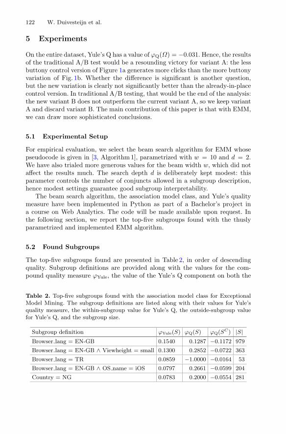
122 W. Duivesteijn et al.
5 Experiments
On the entire dataset, Yule’s Q has a value of ϕQ(Ω) = −0.031. Hence, the resultsof the traditional A/B test would be a resounding victory for variant A: the lessbuttony control version of Figure 1a generates more clicks than the more buttonyvariation of Fig. 1b. Whether the difference is significant is another question,but the new variation is clearly not significantly better than the already-in-placecontrol version. In traditional A/B testing, that would be the end of the analysis:the new variant B does not outperform the current variant A, so we keep variantA and discard variant B. The main contribution of this paper is that with EMM,we can draw more sophisticated conclusions.
5.1 Experimental Setup
For empirical evaluation, we select the beam search algorithm for EMM whosepseudocode is given in [3, Algorithm 1], parametrized with w = 10 and d = 2.We have also trialed more generous values for the beam width w, which did notaffect the results much. The search depth d is deliberately kept modest: thisparameter controls the number of conjuncts allowed in a subgroup description,hence modest settings guarantee good subgroup interpretability.
The beam search algorithm, the association model class, and Yule’s qualitymeasure have been implemented in Python as part of a Bachelor’s project ina course on Web Analytics. The code will be made available upon request. Inthe following section, we report the top-five subgroups found with the thuslyparametrized and implemented EMM algorithm.
5.2 Found Subgroups
The top-five subgroups found are presented in Table 2, in order of descendingquality. Subgroup definitions are provided along with the values for the com-pound quality measure ϕYule, the value of the Yule’s Q component on both the
Table 2. Top-five subgroups found with the association model class for ExceptionalModel Mining. The subgroup definitions are listed along with their values for Yule’squality measure, the within-subgroup value for Yule’s Q, the outside-subgroup valuefor Yule’s Q, and the subgroup size.
Subgroup definition ϕYule(S) ϕQ(S) ϕQ(SC) |S|Browser lang = EN-GB 0.1540 0.1287 −0.1172 979
Browser lang = EN-GB ∧ Viewheight = small 0.1300 0.2852 −0.0722 363
Browser lang = TR 0.0859 −1.0000 −0.0164 53
Browser lang = EN-GB ∧ OS name = iOS 0.0797 0.2661 −0.0599 204
Country = NG 0.0783 0.2000 −0.0554 281

Have It Both Ways—From A/B Testing to A&B Testing 123
subgroup and its complement, and the subgroup size. Recall that the total num-ber of records in the dataset is 3 065, and the value for Yule’s Q on the wholedataset is ϕQ(Ω) = −0.031.
The best subgroup found, S1, is defined by people having British English setas their browser language. More extreme values for Yule’s Q itself can be foundelsewhere in the table; S1 has other distinctive qualities. What sets it apart, isthat there is a clear dichotomy in Q-values between subgroup and complement:the Q-value on S1 is substantially (though not spectacularly) elevated from thebehavior on the whole dataset, and at the same time, the Q-value on the SC
1 issubstantially depressed from the behavior on the whole dataset. This means thatpeople using British English as their browser language generate markedly morerevenue when presented with version B of the web page, whereas people usingany other browser language generate markedly more revenue when presentedwith version A of the web page. Moreover, S1 has a substantial size. These twofactors make S1 the subgroup for which business action is most apposite: wehave clearly distinctive behavior between two sizeable groups of website visitors,and presenting each group with the version of the web page appropriate for thatgroup stands to substantially increase overall revenue.
The second- (S2) and fourth-ranked (S4) subgroups are specializations of S1.S2 specifies visitors that view the website using a relatively small mobile browserscreen; they strongly prefer version B. Small screens can be found in relativelyold smartphones, so this population contains people that are relatively slow inadopting new technology. It stands to reason that this population would alsoprefer a more traditionally-shaped button. S4 specifies visitors that run the iOSoperating system. They too strongly prefer version B, which is remarkable, sincethe buttons of version B do not conform to Apple’s design standards. Perhapsthe unusual button design draws more attention.
The third-ranked subgroup are those people that have set their browser lan-guage to Turkish. This subgroup may be too small to deliver actionable results,covering less than 2% of the dataset. However, the Q-value measured on thissubgroup is strong: this subgroup displays a crystal clear preference for versionA. This is a marked departure from the previously presented subgroups.
The final subgroup presented in Table 2, ranked fifth, concerns people fromNigeria. Yule’s Q indicates that these people prefer version B. Given that theofficial language of Nigeria is English, the version preference is unsurprising: thissubgroup overlaps substantially with S1.
6 Conclusions
Having performed an A/B test—where a pool of test subjects are randomlypresented with either version A or version B of the same product, a measureof success is aggregated by version, and the experimenter is presented with theresults—the typical subsequent action is to make a crisp decision to either main-tain the control version A, or replace it with the new variation version B, whilethe losing alternative is discarded. In this paper, we argue that that action canbe overly coarse. Instead, we present an alternative approach: A&B testing.

124 W. Duivesteijn et al.
The procedure of the A&B test is the exact same as that of a traditionalA/B test, but the subsequent action is much more sophisticated. We analyzethe results of the traditional A/B test with Exceptional Model Mining, to findcoherent subgroups of the overall population that display an unusual responseto the A/B test: the resulting subgroups feature an unusual association betweenthe A/B decision and the measure of success at hand. Hence, while the generalpopulation might generate more revenue when presented with the one version,the resulting subgroups might generate more revenue when presented with theother version. If the company performing the A/B test can afford the upkeep ofboth versions, then knowledge of these subgroups can be invaluable.
As proof of concept, we roll out the A&B test on data generated by Study-Portals, an online information platform for higher education. From the results ofthe A/B test (cf. Fig. 1), we derive several subgroups displaying unusual behav-ior (cf. Table 2). The largest schism lies between people using British Englishas browser language (∼ 1/3 of the population, preferring version B), and peopleusing any other browser language (∼ 2/3 of the population, preferring versionA). In other words, the results suggest that British prefer buttony buttons.
A natural next step would be to verify empirically whether identified sub-groups lead to effective personalization serving either A or B version to corre-sponding web portal visitors. Since it is common for StudyPortals and othercompanies to run a number of A/B testing experiments, and there is a motiva-tion to provide personalized content and personalized layout, it is interesting todevelop a framework for automation of website personalization based on findingsof EMM. It would also make sense to extend this paper by refining the employedquality measure, incorporating the economics of the underlying decision problemdirectly [8].
While the main application within this paper lies in the context of web ana-lytics, it is important to notice that the methodology of A&B testing is applicableon any controlled experiment. Hence, A&B testing is relevant in diverse fieldssuch as medical research [5], education [24], etcetera. In future work, we plan toroll out A&B testing in clinical trials near you.
References
1. Adeyemi, O.: Measures of association for research in educational planning andadministration. Res. J. Math. Stat. 3(3), 82–90 (2010)
2. Duivesteijn, W., Feelders, A., Knobbe, A.J.: Different slopes for different folks –mining for exceptional regression models with cook’s distance. In: Proceedings ofKDD, pp. 868–876 (2012)
3. Duivesteijn, W., Feelders, A.J., Knobbe, A.: Exceptional model mining – super-vised descriptive local pattern mining with complex target concepts. Data Min.Knowl. Disc. 30(1), 47–98 (2016)
4. Hand, D.J.: Pattern detection and discovery. In: Hand, D.J., Adams, N.M., Bolton,R.J. (eds.) Pattern Detection and Discovery. LNCS (LNAI), vol. 2447, pp. 1–12.Springer, Heidelberg (2002). https://doi.org/10.1007/3-540-45728-3 1
Have It Both Ways—From A/B Testing to A&B Testing 125
5. Jakowski, M., Jaroszewicz, S.: Uplift modeling for clinical trial data. In: Proceed-ings of ICML 2012 Workshop on Machine Learning for Clinical Data Analysis(2012)
6. Kohavi, R., Longbotham, R.: Online controlled experiments and A/B tests. In:Sammut, C., Webb, G.I. (eds.) Encyclopedia of Machine Learning and Data Min-ing, pp. 1–8. Springer, New York (2016). https://doi.org/10.1007/978-1-4899-7502-7 891-1
7. Kohavi, R., Longbotham, R., Sommerfield, D., Henne, R.M.: Controlled experi-ments on the web: survey and practical guide. Data Min. Knowl. Discov. 18(1),140–181 (2009)
8. Kleinberg, J., Papadimitrou, C., Raghavan, P.: A microeconomic view of datamining. Data Min. Knowl. Disc. 2(4), 311–324 (1998)
9. Klosgen, W.: Explora: a multipattern and multistrategy discovery assistant. In:Advances in Knowledge Discovery and Data Mining, pp. 249–271 (1996)
10. Krak, T.E., Feelders, A.: Exceptional model mining with tree-constrained gradientascent. In: Proceedings of SDM, pp. 487–495 (2015)
11. Lavrac, N., Kavsek, B., Flach, P.A., Todorovski, L.: Subgroup discovery with CN2-SD. J. Mach. Learn. Res. 5, 153–188 (2004)
12. van Leeuwen, M.: Maximal exceptions with minimal descriptions. Data Min.Knowl. Discov. 21(2), 259–276 (2010)
13. Leman, D., Feelders, A., Knobbe, A.: Exceptional model mining. In: Daelemans,W., Goethals, B., Morik, K. (eds.) ECML PKDD 2008. LNCS (LNAI), vol. 5212,pp. 1–16. Springer, Heidelberg (2008). https://doi.org/10.1007/978-3-540-87481-2 1
14. Lemmerich, F., Becker, M., Atzmueller, M.: Generic pattern trees for exhaustiveexceptional model mining. In: Flach, P.A., De Bie, T., Cristianini, N. (eds.) ECMLPKDD 2012. LNCS (LNAI), vol. 7524, pp. 277–292. Springer, Heidelberg (2012).https://doi.org/10.1007/978-3-642-33486-3 18
15. Mannila, H., Toivonen, H.: Levelwise search and borders of theories in knowledgediscovery. Data Min. Knowl. Discov. 1(3), 241–258 (1997)
16. Moens, S., Boley, M.: Instant exceptional model mining using weighted controlledpattern sampling. In: Blockeel, H., van Leeuwen, M., Vinciotti, V. (eds.) IDA2014. LNCS, vol. 8819, pp. 203–214. Springer, Cham (2014). https://doi.org/10.1007/978-3-319-12571-8 18
17. Morik, K., Boulicaut, J.-F., Siebes, A. (eds.): Local Pattern Detection. Springer,Heidelberg (2005). https://doi.org/10.1007/b137601
18. Rzepakowski, P., Jaroszewicz, S.: Decision trees for uplift modeling with single andmultiple treatments. Knowl. Inf. Syst. 32(2), 303–327 (2012)
19. Rebelo de Sa, C., Duivesteijn, W., Soares, C., Knobbe, A.: Exceptional preferencesmining. In: Calders, T., Ceci, M., Malerba, D. (eds.) DS 2016. LNCS (LNAI), vol.9956, pp. 3–18. Springer, Cham (2016). https://doi.org/10.1007/978-3-319-46307-0 1
20. Siroker, D., Koomen, P.: A/B Testing: The Most Powerful Way to Turn Clicks IntoCustomers. Wiley, Hoboken (2013)
21. StudyPortals. www.studyportals.com22. Tang, L., Jiang, Y., Li, L., Li, T.: Ensemble contextual bandits for personalized
recommendation. In: Proceedings of RecSys, pp. 73–80 (2014)23. Tang, L., Rosales, R., Singh, A.P., Agarwal, D.: Automatic ad format selection via
contextual bandits. In: Proceedings of CIKM, pp. 1587–1594 (2013)

126 W. Duivesteijn et al.
24. Williams, J.J., Li, N., Kim, J., Whitehill, J., Maldonado, S., Pechenizkiy, M.,Chu, L., Heffernan, N.: MOOClets: A Framework for Improving Online Educa-tion through Experimental Comparison and Personalization of Modules. WorkingPaper No. 2523265 (2014). http://tiny.cc/moocletpdf
25. Wrobel, S.: An algorithm for multi-relational discovery of subgroups. In:Komorowski, J., Zytkow, J. (eds.) PKDD 1997. LNCS, vol. 1263, pp. 78–87.Springer, Heidelberg (1997). https://doi.org/10.1007/3-540-63223-9 108
26. Zliobaite, I., Pechenizkiy, M.: Learning with actionable attributes: attention -boundary cases! In: Proceedings of ICDM Workshops, pp. 1021–1028 (2010)
Koopman Spectral Kernels for ComparingComplex Dynamics: Application to Multiagent
Sport Plays
Keisuke Fujii1(B), Yuki Inaba2, and Yoshinobu Kawahara1,3
1 Center for Advanced Intelligence Project, RIKEN, Osaka, [email protected]
2 Japanese Institute of Sports Sciences, Tokyo, [email protected]
3 The Institute of Scientific and Industrial Research, Osaka University, Osaka, [email protected]
Abstract. Understanding the complex dynamics in the real-world suchas in multi-agent behaviors is a challenge in numerous engineering andscientific fields. Spectral analysis using Koopman operators has beenattracting attention as a way of obtaining a global modal description ofa nonlinear dynamical system, without requiring explicit prior knowl-edge. However, when applying this to the comparison or classification ofcomplex dynamics, it is necessary to incorporate the Koopman spectra ofthe dynamics into an appropriate metric. One way of implementing thisis to design a kernel that reflects the dynamics via the spectra. In thispaper, we introduced Koopman spectral kernels to compare the complexdynamics by generalizing the Binet-Cauchy kernel to nonlinear dynam-ical systems without specifying an underlying model. We applied thisto strategic multiagent sport plays wherein the dynamics can be classi-fied, e.g., by the success or failure of the shot. We mapped the latentdynamic characteristics of multiple attacker-defender distances to thefeature space using our kernels and then evaluated the scorability of theplay by using the features in different classification models.
1 Introduction
Groups of organisms competing and cooperating in nature are assumed to behaveas complex and nonlinear dynamical systems, which currently elude formula-tion [7,9]. Understanding the complex dynamics of living organisms or artificialagents (and the component parts) is a challenging research area in biology [5],physics [7], and machine learning. In the field of physics, decomposition or spec-tral methods that factorize the dynamics into modes from the data are used suchas proper orthogonal decomposition (POD) [1,25] or dynamic mode decompo-sition (DMD) [23,24]. The problem of learning dynamical systems in machinelearning has been discussed such as in terms of Bayesian approaches [10] and
c© Springer International Publishing AG 2017Y. Altun et al. (Eds.): ECML PKDD 2017, Part III, LNAI 10536, pp. 127–139, 2017.https://doi.org/10.1007/978-3-319-71273-4_11

128 K. Fujii et al.
predictive state representation [19]. This topic is closely related to the decompo-sition technique in physics, aiming to estimate a prediction model by examiningthe obtained modes.
In this paper, we consider the following discrete-time nonlinear dynamicalsystem:
xt+1 = f (xt) (1)
where xi is a state vector on the state space M (i.e., x ∈ M ⊂ Rd) and f is
a state transition function that assumes the dynamical system to be nonlinear.A recent development is the use of Koopman spectral analysis with reproducingkernels (called kernel DMD). This defines a mode that can yield direct informa-tion about the nonlinear latent dynamics [16]. However, to compare or classifythese complex dynamics, it is necessary to incorporate their Koopman spectruminto a metric appropriate for representing the similarity between the nonlineardynamical systems.
Several works have applied approximation with a low-dimensional linear sub-space to represent this similarity [12,30,33]. One approach has used the Binet-Cauchy (Riemannian) distance with a variety of kernels on a Grassman man-ifold [12], such as the kernel principal angle [33], and the trace and determi-nant kernel [30], which were designed for application in face recognition [33]and movie clustering [30]. The algorithm essentially calculates the Binet-Cauchydistance between two subspaces in the feature space, defined by the productof the canonical correlations. However, the main applications assumed a lineardynamical model [12,30,33] and thus generalization to nonlinear dynamics with-out specifying an underlying model remains to be addressed. In this paper, wemap the latent dynamics to the feature space using the kernels, allowing binaryclassification to be applied to real-world complex dynamical systems.
Organized human group tasks such as navigation [13] or ballgame teams [8]provide excellent examples of complex dynamics and pose challenges in machinelearning because of their switching and overlapping hierarchical subsystems [8],characterized by recursive shared intentionality [28]. Measurement systems havebeen developed that capture information regarding the position of a player in aballgame, allowing analysis of particular shots [11]; however, plays involving col-laboration between several teammates have not yet been addressed. In games suchas basketball or football, coaches analyze team formations and players repeatedlypractice moves that increase the probability of scoring (“scorability”). However,the selection of tactics is an ill-posed problem, and thus basically requires theimplicit experience-based knowledge of the coach. An algorithm is needed thatclarifies scorable moves involving multiple players in the team.
Previous research has classified team moves on a global scale by directlyapplying machine learning methods derived mainly from natural language pro-cessing. These include recursive neural networks (RNN) using optical flow imagesof the trajectories of all players [31] or the application of latent Dirichletallocation (LDA) to the arrangement of individual trajectories [22]. However,the contribution of team movement to the success of a play remains unclear.

Koopman Spectral Kernels for Comparing Complex Dynamics 129
Previously, we reported that three maximum attacker-defender distances sep-arately explained scorability [8], but the study addressed only the outcome ofa play, rather than its time evolution and the interactions that it comprised.An algorithm is required that uses mapping to feature space to discriminatebetween successful and unsuccessful moves while accounting for these complexfactors. In this paper, we map the latent dynamic characteristics of multipleattacker-defender distances [8] to the feature space using our kernels acquiredby kernel DMD and then evaluated scorability.
The rest of the paper is organized as follows. Section 2 briefly reviews thebackground of Koopman spectral kernels, while Sect. 3 discusses methods forcomputing them. We then extended this to empirical example of actual humanlocomotion in Sect. 4. For application to multiple sporting agents, Sect. 5 reportsour findings using the data on actual basketball games. Our approach provedcapable of capturing complex team moves. Finally, Sect. 6 presents our discussionand conclusions.
2 Background
2.1 Koopman Spectral Analysis and Dynamic Mode Decomposition
Spectral analysis (or decomposition) for analyzing dynamical systems is a pop-ular approach aimed at extracting low-dimensional dynamics from the data.Common techniques include global eigenmodes for linearized dynamics, discreteFourier transforms, and POD for nonlinear dynamics [25], as well as multiplevariants of these techniques. DMD has recently attracted particular attention inareas of physics such as fluid mechanics [23] and several engineering fields [2,26]because of its ability to define a mode that can yield direct information evenwhen applied to time series with nonlinear latent dynamics [23,24]. However,the original DMD has numerical disadvantages, related to the accuracy of theapproximate expressions of the Koopman eigenfunctions derived from the data.A number of variants have been proposed to address this shortcoming, includingexact DMD [29], optimized DMD [4], and baysian DMD [27]. Sparsity-promotingDMD [14] provides a framework for the approximation of the Koopman eigen-functions with fewer bases. Extended DMD [32], which works on predeterminedkernel basis functions, has also been proposed. These Koopman spectral analy-ses have been generalized to a reproducing kernel Hilbert space (RKHS) [16], anapproach which is called kernel DMD.
In Koopman spectral analysis, the Koopman operator K [18] is an infinitedimensional linear operator acting on the scalar function gi : M → C. That is,it maps gi to the new function Kgi as follows:
(Kgi) (x) = (gi ◦ f) (x) , (2)

130 K. Fujii et al.
where K denotes the composition of gi with f . We can see that K acts linearlyon the function gi. The dynamics defined by f may be nonlinear. Since K is alinear operator, it can generally perform eigenvalue decomposition:
Kϕj (x) = λjϕj (x) , (3)
where λj ∈ C is the j th eigenvalue (called the Koopman eigenvalue) and ϕj is thecorresponding eigenfunction (called the Koopman eigenfunction). We denote theconcatenation of gj to g := [g1, . . . , gp]T. If each gj lies within the space spannedby the eigenfunction ϕj , we can expand the vector-valued g in terms of theseeigenfunctions as g(x) =
∑∞j=1 ϕj(x)ψj , where ψj is a set of vector coefficients
called Koopman modes. By iterative application of Eqs. (2) and (3), the followingequation is obtained:
(g ◦ f) (x) =∞∑
j=1
λjϕj (x) ψj . (4)
Therefore, λj characterizes the time evolution of the corresponding Koopmanmode ψj , i.e., the phase of λj determines its frequency and the magnitude deter-mines the growth rate of its dynamics.
DMD is a popular approach for estimating the approximations of λj andψj from a finite length observation data sequence y0, y1, . . . , yτ (∈ R
p), whereyt := g(xt). Let A = [y0, y1, . . . , yτ−1] and B = [y1, y2, . . . , yτ ]. Then, DMDbasically approximates those by calculating the eigendecomposition of the least-squares solution to
minP ′∈Rp×p
(1/τ)∑τ
t=0‖yt+1 − P ′yt‖2, (5)
i.e., BA†(:= P ) (•† is the pseudo-inverse of •). Let the j -th right and left eigen-vector of P be ψj and κj , respectively, and assume that these are normalized sothat κ∗
i ψj = δij (δij is the Kronecker’s delta). Then, since any vector b ∈ Cp can
be written as b =∑p
j=1 (κ∗i b)ψj , we have g(x) =
∑pj=1 ϕj(x)ψj by applying it
to g(x). Therefore, by applying K to both sides, we have
(g ◦ f) (x) =p∑
j=1
λjϕj (x) ψj , (6)
indicating a modal representation corresponding to Eq. (4) for the finite sum.
2.2 Kernels for Comparing Nonlinear Dynamical Systems
Selection of an appropriate representation of the data is a fundamental issue inpattern recognition. The important point is to design the features (i.e., kernels)that reflect structure of the data. Time series data is challenging to design thefeatures because of the difficulty in reflecting the data structure (including timelength). Researchers have developed alternative kernel methods, including the

Koopman Spectral Kernels for Comparing Complex Dynamics 131
use of graphs [15,17], subspaces [12,33] or trajectories [30]. In this paper, akernel design applicable to dynamical systems was required. Several methodswere proposed, based on the subspace angle with kernel methods such as foran auto-regressive moving average (ARMA) model [30]. These methodologieswere previously reviewed [12], from the viewpoint of the Riemannian distance(or metric) on the Grassman manifold.
The Grassmann manifold G (m,D) is the set of m-dimensional linear sub-spaces of R
D. Formally, the Riemannian distance between two subspaces isthe geodesic distance on the Grassmann manifold. However, a more intuitiveand computationally efficient way of defining the distances uses the principalangles [20]. A previous review [12] categorized the various Riemannian distancesinto the projection and Binet-Cauchy distance. The former has been used inapplications such as face recognition [3,12], and the latter has been appliedin video clustering [30] and face recognition [33], and has been generalized to(specific nonlinear) dynamical systems [30]. We then adopted the Binet-Cauchydistance when comparing complex systems.
The Binet-Cauchy distances were basically obtained with the product ofcanonical correlations using a variety of kernels [30]. However, the main applica-tions assumed linear dynamical model [12,30,33] such as ARMA model. Thus,it is necessary to generalize to nonlinear dynamics without any specific underly-ing model, into which the Koopman spectrum of dynamics is incorporated. Wecalled the kernels Koopman spectral kernels.
3 Design of Koopman Spectral Kernels
3.1 DMD with Reproducing Kernel
Conceptually, DMD can be considered as producing a local approximation ofthe Koopman eigenfunctions using a set of linear monomials of the observablesas the basis functions. In practice, however, this is certainly not applicable to allsystems (in particular, beyond the region of validity for local linearization). Then,DMD with reproducing kernels [16] approximates the Koopman eigenfunctionswith richer basis functions.
Let H be the RKHS embedded with the dot product determined by a positivedefinite kernel k. Additionally, let φ : M → H be a feature map, and an instanceof φ with respect to x is denoted by φx (i.e., φx := φ(x)). Then, we define theKoopman operator KH : H → H in the RKHS by
KHφx = φx ◦ f . (7)
Note that almost of the theoretical claims in this study do not necessarily requireφ to be in the RKHS (it is sufficient to consider that φ stays within a Hilbertspace), but this assumption should perform the calculation in practice.
In this paper, we robustify the kernel DMD by projecting data onto thedirection of POD [4,16,29]. First, a centered Gram matrix is defined by G =HGH, where G is a Gram matrix, H = I − 1τ , I is a unit matrix, and 1τ is

132 K. Fujii et al.
a τ -by-τ matrix, for which each element takes the value 1/τ . The Gram matrixGxx of the kernel k(yi,yj) is defined at yi and yj (i and j dimensions) of theobservation data matrix A. Similarly, the Gram matrix Gxy of the kernel betweenA and B can be calculated. At this time, Gxx = M∗
τMτ and Gxy = M∗τM+,
where M∗τ indicates the Hermitian transpose of Mτ . Also, Mτ := [φx0 , .., φxτ−1 ]
and M+ := [φx1 , .., φxτ], where φxi
is considered as a feature map of xi fromthe state space M to the RKHS H.
Here, suppose that the eigenvalues and eigenvectors can be truncated based oneigenvalue magnitude. In other words, G ≈ BGB∗ where p (≤ τ) eigenvalues areadopted. Then, a principal orthogonal direction in the feature space is given by
νj = MτHS−1/2jj βj , (8)
where βj is the j th row of B. Let U = [ν1, . . . , νj ] = MτHB S−1/2. Since M+ =KHMτ , the projection of KH onto the space spanned by νj is given as follows:
F = UKHU = S−1/2B∗H(MτM+)HB S−1/2. (9)
Note that Gxy = M∗τM+. Then, if we let F = T−1ΛT be the eigendecomposition
of F , we obtain the centered DMD mode ϕj = Ubj = MτHB S−1/2bj , wherebj is the j th row of T−1. The diagonal matrix Λ comprising the eigenvaluesrepresents the temporal evolution of the mode.
3.2 Koopman Spectral Kernels
For calculating the similarity between the dynamical systems DSi and DSj , wecompute Koopman spectral kernels based on the idea of Binet-Cauchy kernels.The Binet-Cauchy kernels are basically calculated from the traces of compoundmatrices [30] defined as follows. Let M be a matrix in R
m×n. For q ≤ min(m,n),define In
q = {i = i1, · · · , iq : 1 ≤ i1 < ... < iq ≤ n, ii ∈ N}, and likewise Imq . We
denote by Cq(M) the qth compound matrix, that is, the(
mq
)
×(
nq
)
matrix
whose elements are the minors det((Mk,l)k �=i,l�=j ), where i ∈ I nq and j ∈ Imq areassumed to be arranged in lexicographical order. In the unifying viewpoint [30],Binet-Cauchy kernels is a general representation including various kernels [6,15,17,21], divided into two strategies. One is the trace kernel obtained by settingq = 1 (i.e., C1(M) = M), which directly reflects the property of temporalevolution of the dynamical systems, including diffusion kernel [17] and graphkernel [15]. Second is the determinant kernel obtained by setting order q to beequal to the order of the dynamical systems n (i.e., Cn(M) = det(M)), whichextracts coefficients of dynamical systems, including the Martin distance [21]and the distance based on the subspace angle [6].
We expand the kernels to applying Koopman spectral analysis, which arecalled the Koopman trace kernel and Koopman determinant kernel, respectively.Both kernels reflect the Koopman eigenvalue, the eigenfunction, and the mode

Koopman Spectral Kernels for Comparing Complex Dynamics 133
(i.e., system trajectory including the initial condition). However, richer infor-mation of system trajectory does not necessarily increase expressiveness such asin classification with real-world data. Therefore, we also expanded the kernelof principal angle [33] to applying Koopman spectral analysis, which is calledKoopman kernel of principal angle. The kernel principal angle is theoreticallya simple case of the trace kernel [30], which is defined as the inner product oflinear subspaces in this feature space. In this paper, for a simple comparison, wecompute the kernel with the inner product of the Koopman modes (i.e. not thetrajectory and independent of initial condition).
Koopman Trace Kernel and Determinant Kernel. First, for the tracekernel, we generalize the kernel assmuing the ARMA model [30], to nonlineardynamical systems without specifying an underlying model. The trace kernel ofDSi and DSj can be theoretically defined as follows:
k (DSi,DSj) :=∞∑
t=0
(e−κtgi (xi,t)
TWgj (xj ,t)
), (10)
where gi and gj is the observation function and W is an arbitrary semidefinitematrix (here, W = 1). Moreover, for converging the above equation, we supposethe exponential discount μ(t) = e−κt(κ > 0). In this paper, noises in observationand latent dynamics are not considered. Koopman trace kernel can be computedusing the modal representation given by the kernel DMD as follows:
k (DSi,DSj) = ϕi (xi,0)T
∞∑
t=0
(e−κtΛt
i
(Ψi
TWΨj
)Λt
j
)ϕj (xj,0) , (11)
where, Λi is a diagonal matrix consisting of Koopman eigenvalues, Ψi is theKoopman mode, and ϕi is the Koopman eigenfunction (also for j). Althoughthe equation includes an infinite sum, we can efficiently compute the matrixM :=
∑∞t=0 (e−κtΛt
i (ΨTi WΨj )Λt
j ) using the following Sylvester equation M =e−κΛT
i MΛj + ΨTi WΨj , where the Koopman mode Ψ = U∗HMτHU T−1 for i
and j. For creating a trace kernel independent of the initial conditions [30], wetake expectation over xi,0 and xj,0 in the trace kernel, yielding
k (DSi,DSj) = tr(Σϕi(xi,0),ϕj(xj,0)M
), (12)
where the initial Koopman eigenvalue ϕ(x0) = a∗(MτHU)∗Mτ,0 for i andj [16]. Here, a is the left eigenvector of F and Mτ,0 is a vector indicating thefirst single column of Mτ . Σϕi(xi,0),ϕj(xj,0) ∈ C
p×p is the covariance of all initialvalues ϕn (x0) ∈ C
p×n of DSi for each index 1, ... p of eigenvalues (p was fixedfor all i). Similarly, the determinant kernel using the representation given bykernel DMD can be computed:
k (DSi,DSj) = det(ΨiMΨj
T)
, (13)
where M = e−κΛTi MΛj +ϕi(xi,0)ϕj(xj,0)T. Determinant kernels independent
of the initial condition can only be computed for a single output system [30].

134 K. Fujii et al.
Koopman Kernel of Principal Angle. The kernel of principal angle can becomputed using the Koopman modes given by kernel DMD. With respect toDSi, we define the kernel of principal angles as the inner product of the Koop-man modes in the feature space: A∗A = T−1
i U∗i HGxxiHUiTi. If the rank of F
is ri, A∗A is a ri-order square matrix. Also for DSj , we create a similar matrixB∗B. Furthermore, we define the inner product of the linear subspaces betweenDSi and DSj as A∗B = T−1
i U∗i HGxxijHUj Tj . Gxxij is a ni×nj matrix obtained
by picking up the upper-right part of the centered Gram matrix obtained by con-necting Ai and Aj in series (ni and nj are the lengths of the time series). Then,using these matrices, we solve the following generalized eigenvalue problem:
(0 (A∗B)∗
A∗B 0
)
V = λij
(B∗B 0
0 A∗A
)
V , (14)
where the size of λij is finally adjusted to rij = min(ri, rj) in descending order,and V is a generalized eigenvector. The eigenvalue λij is the kernel of principalangle.
4 Embedding and Classification of Dynamics
A direct but important application of this analysis is the embedding and classifi-cation of dynamics using extracted features. A set of Koopman spectra estimatedfrom the analysis can be used as the basis for a low-dimensional subspace rep-resenting the dynamics. The classification of dynamics can be performed usingfeature vectors determined by the Koopman spectral kernels. We used the Gaus-sian kernel, with the kernel width set as the median of the distances from a datamatrix.
Before applying our approach to multiagent sports data, an experiment wasconducted using open-source real-world data. In this case, human locomotiondata were taken from the CMU Graphics Lab Motion Capture Database (avail-able at http://mocap.cs.cmu.edu). To verify the classification performance, wecomputed the trace kernel of an auto-regressive (AR) model, representing a con-ventional linear dynamical model. For embedding of the distance matrix with ourkernels, components of the distance matrix between DSi and DSj in the featurespace were obtained using dist(DSi,DSj) = k(Ai ,Ai)+ k(Aj ,Aj )− 2k(Ai ,Aj ).Figure 1a–c shows the embedding of the sequences using multidimensional scal-ing (MDS) with the distance matrix, computed with the Koopman kernel prin-cipal angle, Koopman determinant kernel, and trace kernel of the AR model,respectively. Classification of performances into jumping, running, and walkingwas computed using the k-nearest neighbor algorithm. Error rates of the testdata were small in this order: the Koopman kernel of principal angle (0.261),Koopman determinant kernel (0.348), trace kernel of the AR model (0.522), andKoopman trace kernel (0.601). Two Koopman spectral kernels performed betterin classification than the kernel of the linear dynamical model.

Koopman Spectral Kernels for Comparing Complex Dynamics 135
-0.5 0 0.5 1-0.5
0
0.5
-1 0 1 2
104
-5000
0
5000
10000
15000
20000
-2 0 2
104
-5000
0
5000
10000
-1000 0 1000
-2000
-1500
-1000
-500
0
-100 0 100-350
-300
-250
-200
-150
-100a b c
Fig. 1. MDS embedding of (a) Koopman kernel of principal angle, (b) Koopman deter-minant kernel, and (c) trace kernel of AR model. Blue, red, and green indicate jump,run, and walk, respectively (x and triangle show the movements with turn and stop,respectively). (Color figure online)
5 Application to Multiagent Sport Plays
We used player-tracking data from two international basketball games in 2015collected by the STATS SportVU system. The total playing time was 80 min,and the total score of the two teams was 276. Positional data comprised the xyposition of every player and the ball on the court, recorded at 25 frames persecond. We eliminated transitions in attack to automatically extract the timeperiods to be analyzed (called an attack-segment). We defined an attack-segmentas the period from all players on the attacking side court entry to 1 s before ashot was made. We analyzed a total of 192 attack-segments, 77 of which endedin a successful shot.
Next, we calculated effective attacker-defender distances to predict the suc-cess or failure of the shot (details were given by [8]), which were temporally andspatially corrected (Fig. 2a). Although all of the distances were 25 dimensions(five attackers and defenders), we previously reduced to four dimensions [8]:(1) ball-mark distance, (2) ball-help distance, (3) pass-mark distance, and (4)pass-help distance (Fig. 2b–c). These distances were used to create seven inputvector series: (i) a one-dimensional distance (1), (ii) a two-dimensional dis-tance comprising (1) and (2), and (iii–iv) three- and four-dimensional (1–3, 1–4)important distances, respectively. For verification, (v) total 25 distances and(vi) 25-dimensional Euclidean distances without spatiotemporal correction werecalculated. We also used (vii) the xy position (total 20 dimensions) of all the tenplayers.
When predicting the outcome of a team-attack movement, it is preferableto compute the posterior probability rather than the outcome identification ofthe shot accuracy itself. We used a naive Bayes classifier and a related vectormachine (RVM) for classification. Figure 3a shows the result of applying thenaive Bayes classifier. The horizontal axis shows the seven input vector series andthe vertical axis the classification error. The Koopman kernel principal anglesderived by inputting four important distances demonstrated minimum error of35.9%. The result of applying the RVM is shown in Fig. 3b, using the same axes.
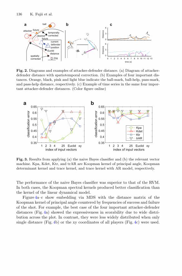
136 K. Fujii et al.
futurecurrentdefenderposition
Euclid distance
attackertemporallycorrected
spatiallycorrected ring
ball
desired
future
0
3
6
Dis
tanc
e
0
3
6
Dis
tanc
e
0 1 2 3 4 5 6 7 8 9 10 11 12 13
time (s)
a b c
Fig. 2. Diagrams and examples of attacker-defender distance. (a) Diagram of attacker-defender distance with spatiotemporal correction. (b) Examples of four important dis-tances. Orange, black, pink and light blue indicate the ball-mark, ball-help, pass-mark,and pass-help distance, respectively. (c) Example of time series in the same four impor-tant attacker-defender distances. (Color figure online)
a b
1 2 3 4 25 Euclid xyindex of input vectors
0.35
0.4
0.45
0.5
0.55
0.6
0.65
clas
sific
atio
n er
ror
1 2 3 4 25 Euclid xyindex of input vectors
0.35
0.4
0.45
0.5
0.55
0.6
0.65
clas
sific
atio
n er
ror
KpaKdetKtrtrAR
Fig. 3. Results from applying (a) the naive Bayes classifier and (b) the relevant vectormachine. Kpa, Kdet, Ktr, and trAR are Koopman kernel of principal angle, Koopmandeterminant kernel and trace kernel, and trace kernel with AR model, respectively.
The performance of the naive Bayes classifier was superior to that of the RVM.In both cases, the Koopman spectral kernels produced better classification thanthe kernel of the linear dynamical model.
Figure 4a–c show embedding via MDS with the distance matrix of theKoopman kernel of principal angle countered by frequencies of success and failureof the shot. For example, the best case of the four important attacker-defenderdistances (Fig. 4a) showed the expressiveness in scorability due to wide distri-bution across the plot. In contrast, they were less widely distributed when onlysingle distance (Fig. 4b) or the xy coordinates of all players (Fig. 4c) were used.
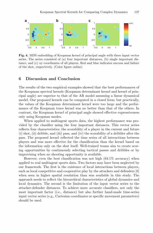
Koopman Spectral Kernels for Comparing Complex Dynamics 137
a b c
-0.5 0 0.5 1-1
-0.5
0
0.5
1
-0.5 0 0.5 1-1
-0.5
0
0.5
1
-0.5 0 0.5 1-1
-0.5
0
0.5
1
fail
succ
Fig. 4. MDS embedding of Koopman kernel of principal angle with three input vectorseries. The series consisted of (a) four important distances, (b) single important dis-tance, and (c) xy coordinates of all players. Red and blue indicates success and failureof the shot, respectively. (Color figure online)
6 Discussion and Conclusion
The results of the two empirical examples showed that the best performances ofthe Koopman spectral kernels (Koopman determinant kernel and kernel of prin-cipal angle) are superior to that of the AR model assuming a linear dynamicalmodel. Our proposed kernels can be computed in a closed form; but practically,the values of the Koopman determinant kernel were too large and the perfor-mance of the Koopman trace kernel was no better than that of the others. Incontrast, the Koopman kernel of principal angle showed effective expressivenessonly using Koopman modes.
When applied to multiagent sports data, the highest performance was pro-vided by the classifier using the four important distances. This vector seriesreflects four characteristics: the scorability of a player in the current and future(i) shot, (ii) dribble, and (iii) pass, and (iv) the scorability of a dribbler after thepass. The proposed kernel reflected the time series of all interactions betweenplayers and was more effective for the classification than the kernel based onthe information only on the shot itself. Well-trained teams aim to create scor-ing opportunities by continuously selecting tactical passes and dribbles or byimprovising when no shooting opportunity is available.
However, even the best classification was not high (64.1% accuracy) whenapplied to real multiagent sports data. Two factors may have been neglected byour framework. The first is the existence of local interactions between players,such as local competitive and cooperative play by the attackers and defenders [8]when seen in higher spatial resolution than was available in this study. Theapproach needs to reflect the hierarchical characteristics of global dynamics andlocal dynamics. The second is the limitation of the input vector series to theattacker-defender distances. To achieve more accurate classifiers, not only themost important factor (i.e., distance) but also further hand-made time-seriesinput vector series (e.g., Cartesian coordinates or specific movement parameters)should be used.

138 K. Fujii et al.
Overall, we developed Koopman spectral kernels that can be computed inclosed form and used to compare multiple nonlinear dynamical systems. In com-petitive sports, coaches spend considerable amounts of time analyzing videos oftheir own team and the opposing team. Application of a system such as the onepresented here may save time and create tactical plans that can currently begenerated only by experienced coaches. More generally, the algorithm can beapplied to the analysis of the complex dynamics of groups of living organismsor artificial agents, which currently elude formulation.
Acknowledgements. We would like to thank Charlie Rohlf and the STATS team fortheir help and support for this work. This work was supported by JSPS KAKENHIGrant Numbers 16H01548.
References
1. Bonnet, J., Cole, D., Delville, J., Glauser, M., Ukeiley, L.: Stochastic estimationand proper orthogonal decomposition: complementary techniques for identifyingstructure. Exp. Fluids 17(5), 307–314 (1994)
2. Brunton, B.W., Johnson, L.A., Ojemann, J.G., Kutz, J.N.: Extracting spatial-temporal coherent patterns in large-scale neural recordings using dynamic modedecomposition. J. Neurosci. Methods 258, 1–15 (2016)
3. Chang, J.M., Beveridge, J.R., Draper, B.A., Kirby, M., Kley, H., Peterson, C.: Illu-mination face spaces are idiosyncratic. In: Proceedings of International Conferenceon Image Processing, Computer Vision, & Pattern Recognition, vol. 2, pp. 390–396(2006)
4. Chen, K.K., Tu, J.H., Rowley, C.W.: Variants of dynamic mode decomposition:boundary condition, Koopman, and Fourier analyses. J. Nonlinear Sci. 22(6), 887–915 (2012)
5. Couzin, I.D., Krause, J., Franks, N.R., Levin, S.A.: Effective leadership anddecision-making in animal groups on the move. Nature 433(7025), 513–516 (2005)
6. De Cock, K., De Moor, B.: Subspace angles between ARMA models. Syst. ControlLett. 46(4), 265–270 (2002)
7. Fodor, E., Nardini, C., Cates, M.E., Tailleur, J., Visco, P., van Wijland, F.: Howfar from equilibrium is active matter? Phys. Rev. Lett. 117(3), 038103 (2016)
8. Fujii, K., Yokoyama, K., Koyama, T., Rikukawa, A., Yamada, H., Yamamoto, Y.:Resilient help to switch and overlap hierarchical subsystems in a small humangroup. Scientific Reports 6 (2016)
9. Fujii, K., Isaka, T., Kouzaki, M., Yamamoto, Y.: Mutual and asynchronous antici-pation and action in sports as globally competitive and locally coordinative dynam-ics. Scientific Reports 5 (2015)
10. Ghahramani, Z., Roweis, S.T.: Learning nonlinear dynamical systems using an EMalgorithm. In: Advances in Neural Information Processing Systems, pp. 431–437(1999)
11. Goldman, M., Rao, J.M.: Live by the three, die by the three? The price of risk inthe NBA. In: Proceedings of MIT Sloan Sports Analytics Conference (2013)
12. Hamm, J., Lee, D.D.: Grassmann discriminant analysis: a unifying view onsubspace-based learning. In: Proceedings of International Conference on MachineLearning, pp. 376–383 (2008)
Koopman Spectral Kernels for Comparing Complex Dynamics 139
13. Hutchins, E.: The technology of team navigation. In: Intellectual Teamwork: Socialand Technological Foundations of Cooperative Work, vol. 1, pp. 191–220 (1990)
14. Jovanovic, M.R., Schmid, P.J., Nichols, J.W.: Sparsity-promoting dynamic modedecomposition. Phys. Fluids 26(2), 024103 (2014)
15. Kashima, H., Tsuda, K., Inokuchi, A.: Kernels for graphs. Kernel Methods Comput.Biol. 39(1), 101–113 (2004)
16. Kawahara, Y.: Dynamic mode decomposition with reproducing kernels for Koop-man spectral analysis. In: Proceedings of Advances in Neural Information Process-ing Systems, pp. 911–919 (2016)
17. Kondor, R.I., Lafferty, J.: Diffusion kernels on graphs and other discrete inputspaces. In: Proceedings of International Conference on Machine Learning, vol. 2,pp. 315–322 (2002)
18. Koopman, B.O.: Hamiltonian systems and transformation in Hilbert space. Proc.Natl. Acad. Sci. 17(5), 315–318 (1931)
19. Kulesza, A., Jiang, N., Singh, S.P.: Spectral learning of predictive state represen-tations with insufficient statistics. In: Proceedings of Association for the Advance-ment of Artificial Intelligence, pp. 2715–2721 (2015)
20. Loan, C.V., Golub, G.: Matrix Computations, 3rd edn. Johns Hopkins UniversityPress, Baltimore (1996)
21. Martin, R.J.: A metric for ARMA processes. IEEE Trans. Signal Process. 48(4),1164–1170 (2000)
22. Miller, A.C., Bornn, L.: Possession sketches: mapping NBA strategies (2017)23. Rowley, C.W., Mezic, I., Bagheri, S., Schlatter, P., Henningson, D.S.: Spectral
analysis of nonlinear flows. J. Fluid Mech. 641, 115–127 (2009)24. Schmid, P.J.: Dynamic mode decomposition of numerical and experimental data.
J. Fluid Mech. 656, 5–28 (2010)25. Sirovich, L.: Turbulence and the dynamics of coherent structures. I. Coherent struc-
tures. Q. Appl. Math. 45(3), 561–571 (1987)26. Susuki, Y., Mezic, I.: Nonlinear koopman modes and power system stability assess-
ment without models. IEEE Trans. Power Syst. 29(2), 899–907 (2014)27. Takeishi, N., Kawahara, Y., Tabei, Y., Yairi, T.: Bayesian dynamic mode decom-
position. In: Proceedings of the International Joint Conference on Artificial Intel-ligence (2017)
28. Tomasello, M., Carpenter, M.: Shared intentionality. Dev. Sci. 10(1), 121–125(2007)
29. Tu, J.H., Rowley, C.W., Luchtenburg, D.M., Brunton, S.L., Kutz, J.N.: Ondynamic mode decomposition: theory and applications. J. Comput. Dyn. 1(2),391–421 (2014)
30. Vishwanathan, S., Smola, A.J., Vidal, R.: Binet-Cauchy kernels on dynamical sys-tems and its application to the analysis of dynamic scenes. Int. J. Comput. Vis.73(1), 95–119 (2007)
31. Wang, K.C., Zemel, R.: Classifying NBA offensive plays using neural networks. In:Proceedings of MIT Sloan Sports Analytics Conference (2016)
32. Williams, M.O., Kevrekidis, I.G., Rowley, C.W.: A data-driven approximation ofthe Koopman operator: extending dynamic mode decomposition. J. Nonlinear Sci.25(6), 1307–1346 (2015)
33. Wolf, L., Shashua, A.: Learning over sets using kernel principal angles. J. Mach.Learn. Res. 4, 913–931 (2003)

Modeling the Temporal Nature of HumanBehavior for Demographics Prediction
Bjarke Felbo1,3, Pal Sundsøy2, Alex ‘Sandy’ Pentland1, Sune Lehmann3,and Yves-Alexandre de Montjoye1,4(B)
1 MIT Media Lab, Massachusetts Institute of Technology, Cambridge, USA2 Telenor Research, Oslo, Norway
3 DTU Compute, Technical University of Denmark, Kgs. Lyngby, Denmark4 Department of Computing and Data Science Institute,
Imperial College London, London, [email protected]
Abstract. Mobile phone metadata is increasingly used for humanitar-ian purposes in developing countries as traditional data is scarce. Basicdemographic information is however often absent from mobile phonedatasets, limiting the operational impact of the datasets. For these rea-sons, there has been a growing interest in predicting demographic infor-mation from mobile phone metadata. Previous work focused on creatingincreasingly advanced features to be modeled with standard machinelearning algorithms. We here instead model the raw mobile phone meta-data directly using deep learning, exploiting the temporal nature of thepatterns in the data. From high-level assumptions we design a data rep-resentation and convolutional network architecture for modeling patternswithin a week. We then examine three strategies for aggregating patternsacross weeks and show that our method reaches state-of-the-art accuracyon both age and gender prediction using only the temporal modality inmobile metadata. We finally validate our method on low activity usersand evaluate the modeling assumptions.
Keywords: Call Detail Records · Mobile phone metadataTemporal patterns · User modeling · Demographics prediction
1 Introduction
For the first time last year, there were more active mobile phones in the worldthan humans [17]. Every time one of these phones is being used to text or call,it generates mobile phone metadata or CDR (Call Detail Records). Collected atlarge scale this metadata – records of who calls or texts whom, for how long, andfrom where – provide a unique lens into the behavior of humans and societies.For instance, mobile phone metadata have been used to plan disaster responseand inform public health policy [2,24]. The potential of mobile phone metadatais particularly high in developing countries where basic statistics such as popula-tion density or mobility are often either missing or suffer from severe biases [21].c© Springer International Publishing AG 2017Y. Altun et al. (Eds.): ECML PKDD 2017, Part III, LNAI 10536, pp. 140–152, 2017.https://doi.org/10.1007/978-3-319-71273-4_12
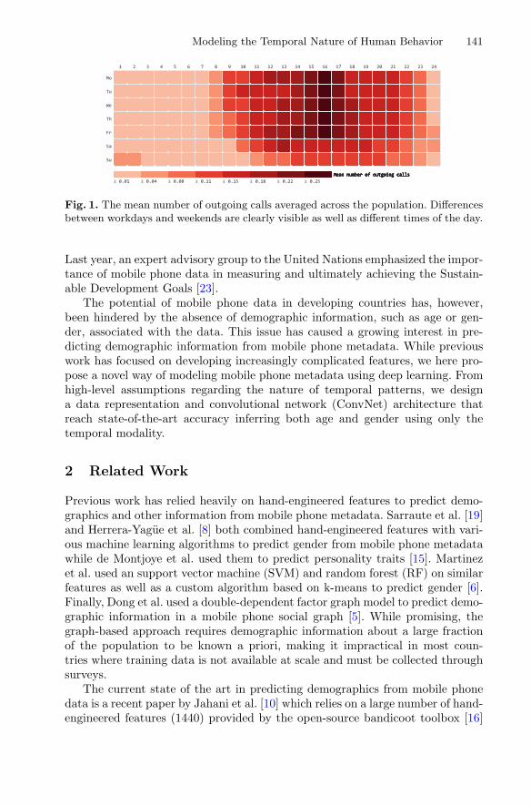
Modeling the Temporal Nature of Human Behavior 141
Fig. 1. The mean number of outgoing calls averaged across the population. Differencesbetween workdays and weekends are clearly visible as well as different times of the day.
Last year, an expert advisory group to the United Nations emphasized the impor-tance of mobile phone data in measuring and ultimately achieving the Sustain-able Development Goals [23].
The potential of mobile phone data in developing countries has, however,been hindered by the absence of demographic information, such as age or gen-der, associated with the data. This issue has caused a growing interest in pre-dicting demographic information from mobile phone metadata. While previouswork has focused on developing increasingly complicated features, we here pro-pose a novel way of modeling mobile phone metadata using deep learning. Fromhigh-level assumptions regarding the nature of temporal patterns, we designa data representation and convolutional network (ConvNet) architecture thatreach state-of-the-art accuracy inferring both age and gender using only thetemporal modality.
2 Related Work
Previous work has relied heavily on hand-engineered features to predict demo-graphics and other information from mobile phone metadata. Sarraute et al. [19]and Herrera-Yague et al. [8] both combined hand-engineered features with vari-ous machine learning algorithms to predict gender from mobile phone metadatawhile de Montjoye et al. used them to predict personality traits [15]. Martinezet al. used an support vector machine (SVM) and random forest (RF) on similarfeatures as well as a custom algorithm based on k-means to predict gender [6].Finally, Dong et al. used a double-dependent factor graph model to predict demo-graphic information in a mobile phone social graph [5]. While promising, thegraph-based approach requires demographic information about a large fractionof the population to be known a priori, making it impractical in most coun-tries where training data is not available at scale and must be collected throughsurveys.
The current state of the art in predicting demographics from mobile phonedata is a recent paper by Jahani et al. [10] which relies on a large number of hand-engineered features (1440) provided by the open-source bandicoot toolbox [16]

142 B. Felbo et al.
and a carefully tuned SVM with a radial basis function kernel. The featuresused are divided into two categories (individual, spatial) and based on carefullyengineered definitions such as how to group together calls and text messages intoconversations or compute the churn rate of common locations.
3 Data and Assumptions
A mobile phone produces a record every time it sends or receives a text messageor makes or receives a phone call. These records (called mobile phone metadata,or CDRs) are generated by the carrier’s infrastructure and are highly stan-dardized. CDRs contain the type of interaction (text/call), direction (in/out),timestamp (date and time), recipient ID, call duration (if call) and cell tower towhich the phone was connected to. The dataset we work with, provided by ananonymous carrier, contains more than 250 million anonymized mobile phonerecords for 150.000 people in a Western European country covering a period of14 weeks.
We state the following three assumptions about the nature of the temporalpatterns in mobile phone metadata:
1. The day of the week and time of day of an observed pattern holdspredictive powerPrevious work showed that increasing the temporal granularity of the hand-engineered features in the bandicoot toolbox by differentiating between day-time and nighttime activity yields a substantial accuracy boost [10]. Forinstance, the percentage of initiated calls at night during the weekend wasone of the most useful features to predict gender. Consequently, we assumethat information on the specific time of the week that a pattern occurredcontains useful information to predict demographic attributes.
2. Temporal patterns are similar across days of the weekWhile the time of day matters (e.g. night vs. day), we furthermore assumethat such temporal patterns have similarities across days of the week whichcould help predict demographic attributes. For instance, one could imaginethat a relevant temporal pattern on Friday night may help model a similarpattern on Saturday night.
3. Local temporal patterns can be combined into predictive globalfeaturesThe current state-of-the-art approach relies on complex hand-engineered (andnon-linear) features such as the response rate within conversations, churnbetween antennas, and entropy of contacts [10]. We assume that the convo-lutional network (ConvNet) will be able to combine local temporal patternson the scale of hours to find global features (i.e. on the scale of days/weeks),thereby removing the need for such high-level hand-engineered features.ConvNets have similarly been used in previous work to learn a hierarchyof features directly from raw visual data [13].

Modeling the Temporal Nature of Human Behavior 143
4 Representation, Architecture and Aggregation
4.1 Week-Matrix Representation
Assumptions 1 and 2 from Sect. 3 are used to derive our data representationfor a week of mobile phone metadata. We represent the data as eight matricessummarizing mobile phone usage on a given week with hours of the day on thex-axis and the weekdays on the y-axis (see Fig. 1). These eight matrices are thenumber of unique contacts, calls, texts and the total duration of calls for incom-ing and outgoing interactions respectively. Every cell in the matrices representsthe amount of activity for a given variable of interest in that hour interval (e.g.between 2 and 3 pm). In this way, we effectively bin any number of interac-tions during the week. These eight matrices are combined into a 3-dimensionalmatrix with a separate ‘channel’ for each of the 8 variables of interest. This3-dimensional matrix is named a ‘week-matrix’.
The week-matrix representation is a logical result of our Assumptions 1 and2. Our first assumption focuses on the importance of high temporal granularity,which is why our data representation summarizes mobile phone usage for eachhour, thereby splitting local patterns into separate bins such that they may becaptured by a suitable classification algorithm. Our second assumption focuseson the similarity of temporal patterns across weekdays, making it logical todesign the week-matrix to have the weekdays on the y-axis such that similarpatterns are located in neighboring cells in the matrix (see Fig. 1 for clear tem-poral patterns in mobile phone usage across weekdays). We shift the time in thematrices by 4 h such that it is easier to capture mobile phone usage occurringacross midnight (Fig. 1 shows that there is especially a lot of activity occurringthe night between Saturday and Sunday). Each row in the matrix thus containsdata from 4 am–4 am instead of from midnight to midnight. This shift alsomoves the low-activity (and potentially less informative) areas to the borders ofthe matrix.
4.2 ConvNet Architecture
We use our assumptions (see Sect. 3) to develop the ConvNet architecture usedto model a single week of mobile metadata. The choice of architecture is crucialto finding predictive patterns and has been equated to a choice of prior [1].
Assumption 2 emphasizes the similarity of temporal patterns across week-days. We therefore design an architecture consisting of five horizontal conv. layersfollowed by a vertical conv. filter and a dense layer (see Table 1 and Fig. 2). Thehorizontal conv. layers learn to capture patterns within a single day, reusing thesame parameters across different times of day and across the different weekdays.For a 1D conv. filter with filter size four (as illustrated in Fig. 2) the value of asingle neuron at the position k in the next layer is:
ok = σ
(b +
3∑l=0
wlik+l
), (1)
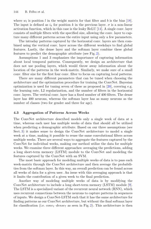
144 B. Felbo et al.
where wl is position l in the weight matrix for that filter and b is the bias [18].The input is defined as ik for position k in the previous layer. σ is a non-linearactivation function, which in this case is the leaky ReLU [14]. A single conv. layerconsists of multiple filters with the specified size, allowing the conv. layer to cap-ture many different patterns across the entire input using only a few parameters.
The intraday patterns captured by the horizontal conv. layers are then com-bined using the vertical conv. layer across the different weekdays to find globalfeatures. Lastly, the dense layer and the softmax layer combine these globalfeatures to predict the demographic attribute (see Fig. 2).
Assumptions 1 and 3 emphasizes the importance of capturing informationabout local temporal patterns. Consequently, we design an architecture thatdoes not use pooling layers, which would throw away information about thelocation of the patterns in the week-matrix. Similarly, we make sure of a smallconv. filter size for the first four conv. filter to focus on capturing local patterns.
There are many different parameters that can be tuned when choosing thearchitecture and the optimization procedure for training the ConvNet. Bayesianoptimization is used for tuning seven of these as proposed in [20], covering e.g.the learning rate, L2 regularization, and the number of filters in the horizontalconv. layers. The vertical conv. layer has a fixed number of 400 filters. The denselayer has 400 neurons, whereas the softmax layer has as many neurons as thenumber of classes (two for gender and three for age).
4.3 Aggregation of Patterns Across Weeks
The ConvNet architecture described models only a single week of data at atime, whereas each user has multiple weeks of data that should all be utilizedwhen predicting a demographic attribute. Based on our three assumptions (seeSect. 3) it makes sense to design the ConvNet architecture to model a singleweek at a time, making it possible to reuse the same convolutional filters acrossmultiple weeks. There are several ways to aggregate the features captured by theConvNet for individual weeks, making our method utilize the data for multipleweeks. We examine three different approaches: averaging the predictions, addinga long short-term memory (LSTM) module to the ConvNet and modeling thefeatures captured by the ConvNet with an SVM.
The most basic approach for modeling multiple weeks of data is to pass eachweek-matrix through the ConvNet architecture and then average the probabili-ties from the softmax layer. In this way, an overall prediction can be found acrossall weeks of data for a given user. An issue with this averaging approach is thatit limits the contribution of a given week to the final prediction.
Another way of modeling multiple weeks of data is by modifying theConvNet architecture to include a long short-term memory (LSTM) module [9].The LSTM is a specialized variant of the recurrent neural network (RNN), whichuses recurrent connections between the neurons to capture patterns in sequencesof inputs. We design a ConvNet-LSTM such that it has the same architecture forfinding patterns as our ConvNet architecture, but without the final softmax layerfor classification (i.e. conv1–dense7 as seen in Fig. 2). This architecture is then
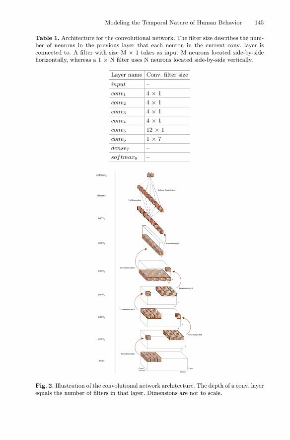
Modeling the Temporal Nature of Human Behavior 145
Table 1. Architecture for the convolutional network. The filter size describes the num-ber of neurons in the previous layer that each neuron in the current conv. layer isconnected to. A filter with size M × 1 takes as input M neurons located side-by-sidehorizontally, whereas a 1 × N filter uses N neurons located side-by-side vertically.
Layer name Conv. filter size
input –
conv1 4 × 1
conv2 4 × 1
conv3 4 × 1
conv4 4 × 1
conv5 12 × 1
conv6 1 × 7
dense7 –
softmax8 –
7 days
24 hours
8 inputchannels
7
21
7
12
7
1
M F
Convolution (4x1)
Convolution (12x1)
Softmax Classification
Convolution (1x7)
Full Connection
input
conv1
conv3
conv5
conv6
dense7
softmax8
Convolution (4x1)
7
18
7
15
Convolution (4x1)
Convolution (4x1)
conv2
conv4
Fig. 2. Illustration of the convolutional network architecture. The depth of a conv. layerequals the number of filters in that layer. Dimensions are not to scale.
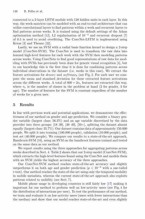
146 B. Felbo et al.
connected to a 2-layer LSTM module with 128 hidden units in each layer. In thisway, the week-matrices can be modeled with an end-to-end architecture that canutilize convolutional layers to find patterns within a week and recurrent layers tofind patterns across weeks. It is trained using the default settings of the Adamoptimization method [12]. L2 regularization of 10−4 and recurrent dropout [7]of 0.5 is used to avoid overfitting. The ConvNet-LSTM is implemented usingKeras [3] and Theano [22].
Lastly, we use an SVM with a radial basis function kernel to design a 2-stepmodel (ConvNet-SVM). The ConvNet is used to transform the raw data intolearned high-level features for each week with the SVM then modeling patternsacross weeks. Using ConvNets to find good representations of raw data for mod-eling with SVMs has previously been done for generic visual recognition [4], butto our knowledge this is the first time it is done for combining patterns acrossindividual observations in the dataset (i.e. weeks in this case). We extract thefeature activations for dense7 and softmax8 (see Fig. 2. For each user we com-pute the mean and standard deviation for these extracted feature activationsacross the different weeks. A total of 800 + 2nc features are extracted this way,where nc is the number of classes in the problem at hand (2 for gender, 3 forage). The number of features for the SVM is constant regardless of the numberof weeks for a given user.
5 Results
In line with previous work and potential applications, we demonstrate the effec-tiveness of our method on gender and age prediction. We consider a binary gen-der variable (largest class: 56.3%) and an age variable discretized by the dataprovider into three groups: [18–39], [40–49], [50+], splitting the dataset almostequally (largest class: 35.7%). Our dataset contains data of approximately 150.000people. We split it into training (100.000 people), validation (10.000 people), andtest set (40.000 people). We compare our results to a state-of-the-art approach,Bandicoot-SVM [10], using an SVM on the bandicoot features trained and testedon the same data as our method.
We report results using the three approaches for aggregating patterns acrossweeks described in Sect. 4. Table 2 shows that our 2-step model (ConvNet-SVM),which extracts the high-level features found using the ConvNet and models themwith an SVM yields the highest accuracy of the three approaches.
Our ConvNet-SVM method reaches state-of-the-art accuracy and slightlyoutperforms it on both age and gender prediction (p < 10−5 with a one-tailedt-test). Our method reaches the state-of-the-art using only the temporal modalityin mobile metadata, whereas the current state-of-the-art approach also exploitspatterns related to mobility (see Sect. 7).
Mobile phone usage in developing countries is still fairly low [17] making itimportant for our method to perform well on low-activity users (see Fig. 4 forthe distribution of interactions per user). To test the performance of our method,we train and evaluate it on low-activity users (users with fewer interactions thanthe median) and show that our model reaches state-of-the-art and even slightly
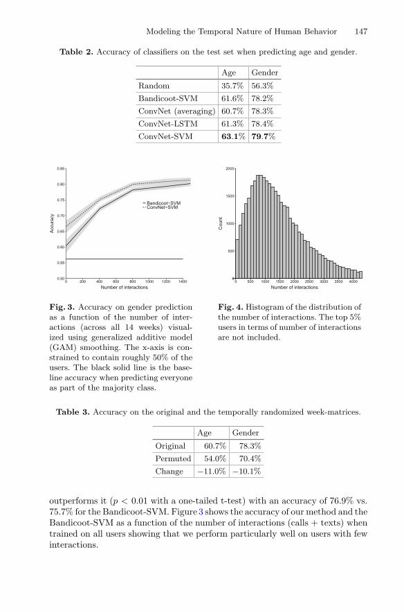
Modeling the Temporal Nature of Human Behavior 147
Table 2. Accuracy of classifiers on the test set when predicting age and gender.
Age Gender
Random 35.7% 56.3%
Bandicoot-SVM 61.6% 78.2%
ConvNet (averaging) 60.7% 78.3%
ConvNet-LSTM 61.3% 78.4%
ConvNet-SVM 63.1% 79.7%
0.50
0.55
0.60
0.65
0.70
0.75
0.80
0.85
0 200 400 600 800 1000 1200 1400Number of interactions
Accu
racy
Bandicoot−SVMConvNet−SVM
Fig. 3. Accuracy on gender predictionas a function of the number of inter-actions (across all 14 weeks) visual-ized using generalized additive model(GAM) smoothing. The x-axis is con-strained to contain roughly 50% of theusers. The black solid line is the base-line accuracy when predicting everyoneas part of the majority class.
0
500
1000
1500
2000
0 500 1000 1500 2000 2500 3000 3500 4000Number of interactions
Cou
nt
Fig. 4. Histogram of the distribution ofthe number of interactions. The top 5%users in terms of number of interactionsare not included.
Table 3. Accuracy on the original and the temporally randomized week-matrices.
Age Gender
Original 60.7% 78.3%
Permuted 54.0% 70.4%
Change −11.0% −10.1%
outperforms it (p < 0.01 with a one-tailed t-test) with an accuracy of 76.9% vs.75.7% for the Bandicoot-SVM. Figure 3 shows the accuracy of our method and theBandicoot-SVM as a function of the number of interactions (calls + texts) whentrained on all users showing that we perform particularly well on users with fewinteractions.
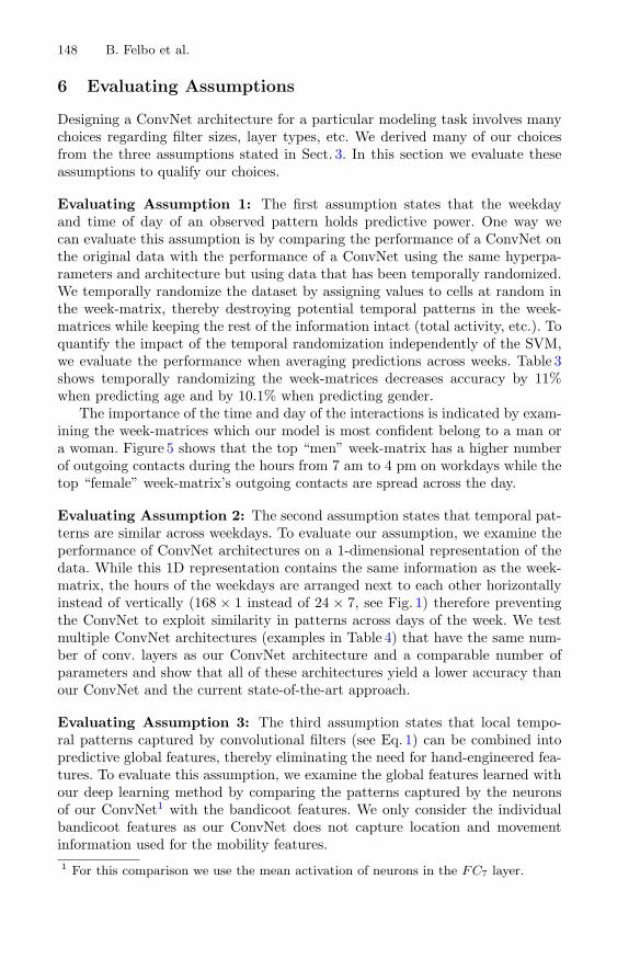
148 B. Felbo et al.
6 Evaluating Assumptions
Designing a ConvNet architecture for a particular modeling task involves manychoices regarding filter sizes, layer types, etc. We derived many of our choicesfrom the three assumptions stated in Sect. 3. In this section we evaluate theseassumptions to qualify our choices.
Evaluating Assumption 1: The first assumption states that the weekdayand time of day of an observed pattern holds predictive power. One way wecan evaluate this assumption is by comparing the performance of a ConvNet onthe original data with the performance of a ConvNet using the same hyperpa-rameters and architecture but using data that has been temporally randomized.We temporally randomize the dataset by assigning values to cells at random inthe week-matrix, thereby destroying potential temporal patterns in the week-matrices while keeping the rest of the information intact (total activity, etc.). Toquantify the impact of the temporal randomization independently of the SVM,we evaluate the performance when averaging predictions across weeks. Table 3shows temporally randomizing the week-matrices decreases accuracy by 11%when predicting age and by 10.1% when predicting gender.
The importance of the time and day of the interactions is indicated by exam-ining the week-matrices which our model is most confident belong to a man ora woman. Figure 5 shows that the top “men” week-matrix has a higher numberof outgoing contacts during the hours from 7 am to 4 pm on workdays while thetop “female” week-matrix’s outgoing contacts are spread across the day.
Evaluating Assumption 2: The second assumption states that temporal pat-terns are similar across weekdays. To evaluate our assumption, we examine theperformance of ConvNet architectures on a 1-dimensional representation of thedata. While this 1D representation contains the same information as the week-matrix, the hours of the weekdays are arranged next to each other horizontallyinstead of vertically (168 × 1 instead of 24 × 7, see Fig. 1) therefore preventingthe ConvNet to exploit similarity in patterns across days of the week. We testmultiple ConvNet architectures (examples in Table 4) that have the same num-ber of conv. layers as our ConvNet architecture and a comparable number ofparameters and show that all of these architectures yield a lower accuracy thanour ConvNet and the current state-of-the-art approach.
Evaluating Assumption 3: The third assumption states that local tempo-ral patterns captured by convolutional filters (see Eq. 1) can be combined intopredictive global features, thereby eliminating the need for hand-engineered fea-tures. To evaluate this assumption, we examine the global features learned withour deep learning method by comparing the patterns captured by the neuronsof our ConvNet1 with the bandicoot features. We only consider the individualbandicoot features as our ConvNet does not capture location and movementinformation used for the mobility features.1 For this comparison we use the mean activation of neurons in the FC7 layer.
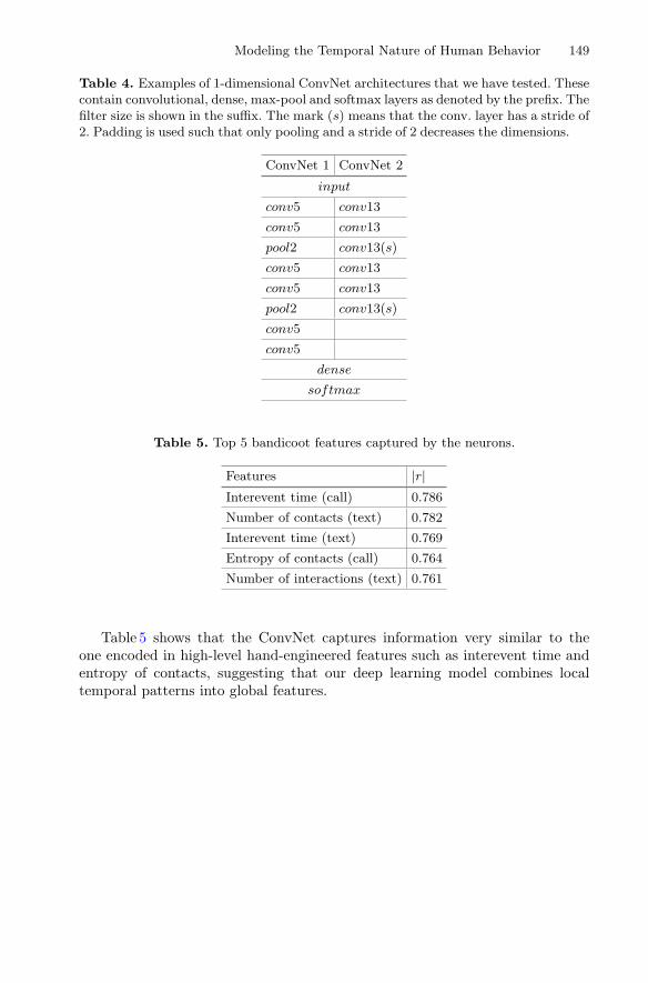
Modeling the Temporal Nature of Human Behavior 149
Table 4. Examples of 1-dimensional ConvNet architectures that we have tested. Thesecontain convolutional, dense, max-pool and softmax layers as denoted by the prefix. Thefilter size is shown in the suffix. The mark (s) means that the conv. layer has a stride of2. Padding is used such that only pooling and a stride of 2 decreases the dimensions.
ConvNet 1 ConvNet 2
input
conv5 conv13
conv5 conv13
pool2 conv13(s)
conv5 conv13
conv5 conv13
pool2 conv13(s)
conv5
conv5
dense
softmax
Table 5. Top 5 bandicoot features captured by the neurons.
Features |r|Interevent time (call) 0.786
Number of contacts (text) 0.782
Interevent time (text) 0.769
Entropy of contacts (call) 0.764
Number of interactions (text) 0.761
Table 5 shows that the ConvNet captures information very similar to theone encoded in high-level hand-engineered features such as interevent time andentropy of contacts, suggesting that our deep learning model combines localtemporal patterns into global features.
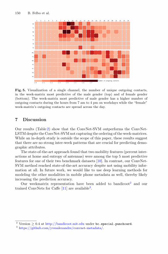
150 B. Felbo et al.
Fig. 5. Visualization of a single channel, the number of unique outgoing contacts,in the week-matrix most predictive of the male gender (top) and of female gender(bottom). The week-matrix most predictive of male gender has a higher number ofoutgoing contacts during the hours from 7 am to 4 pm on workdays while the “female”week-matrix’s outgoing contacts are spread across the day.
7 Discussion
Our results (Table 2) show that the ConvNet-SVM outperforms the ConvNet-LSTM despite the ConvNet-SVM not capturing the ordering of the week-matrices.While an in-depth study is outside the scope of this paper, these results suggestthat there are no strong inter-week patterns that are crucial for predicting demo-graphic attributes.
The state-of-the-art approach found that two mobility features (percent inter-actions at home and entropy of antennas) were among the top 5 most predictivefeatures for one of their two benchmark datasets [10]. In contrast, our ConvNet-SVM method reached state-of-the-art accuracy despite not using mobility infor-mation at all. In future work, we would like to use deep learning methods formodeling the other modalities in mobile phone metadata as well, thereby likelyincreasing the prediction accuracy.
Our weekmatrix representation have been added to bandicoot2 and ourtrained ConvNets for Caffe [11] are available3.
2 Version ≥ 0.4 at http://bandicoot.mit.edu under bc.special.punchcard.3 https://github.com/yvesalexandre/convnet-metadata/.
Modeling the Temporal Nature of Human Behavior 151
References
1. Bengio, Y., Courville, A., Vincent, P.: Representation learning: a review and newperspectives. TPAMI 35(8), 1798–1828 (2013)
2. Bengtsson, L., Lu, X., Thorson, A., Garfield, R., Von Schreeb, J.: Improvedresponse to disasters and outbreaks by tracking population movements with mobilephone network data: a post-earthquake geospatial study in Haiti. PLoS Med. 8(8),e1001083 (2011)
3. Chollet, F.: keras (2015). https://github.com/fchollet/keras4. Donahue, J., Jia, Y., Vinyals, O., Hoffman, J., Zhang, N., Tzeng, E., Darrell, T.:
Decaf: a deep convolutional activation feature for generic visual recognition. In:PMLR. arXiv arXiv:1310.1531 (2013)
5. Dong, Y., Yang, Y., Tang, J., Yang, Y., Chawla, N.V.: Inferring user demographicsand social strategies in mobile social networks. In: Proceedings of the 20th ACMSIGKDD International Conference on Knowledge Discovery and Data Mining, pp.15–24. ACM (2014)
6. Frias-Martinez, V., Frias-Martinez, E., Oliver, N.: A gender-centric analysis ofcalling behavior in a developing economy using call detail records. In: AAAI SpringSymposium: Artificial Intelligence for Development (2010)
7. Gal, Y.: A theoretically grounded application of dropout in recurrent neural net-works. In: NIPS. arXiv arXiv:1512.05287 (2016)
8. Herrera-Yague, C., Zufiria, P.J.: Prediction of telephone user attributes basedon network neighborhood information. In: Perner, P. (ed.) MLDM 2012. LNCS(LNAI), vol. 7376, pp. 645–659. Springer, Heidelberg (2012). https://doi.org/10.1007/978-3-642-31537-4 50
9. Hochreiter, S., Schmidhuber, J.: Long short-term memory. Neural Comput. 9(8),1735–1780 (1997)
10. Jahani, E., Sundsøy, P., Bjelland, J., Bengtsson, L., de Montjoye, Y.A., et al.:Improving official statistics in emerging markets using machine learning and mobilephone data. EPJ Data Sci. 6(1), 3 (2017)
11. Jia, Y., Shelhamer, E., Donahue, J., Karayev, S., Long, J., Girshick, R., Guadar-rama, S., Darrell, T.: Caffe: Convolutional architecture for fast feature embedding.arXiv arXiv:1408.5093 (2014)
12. Kingma, D., Ba, J.: Adam: a method for stochastic optimization. In: ICLR. arXivarXiv:1412.6980 (2015)
13. LeCun, Y., Bengio, Y., Hinton, G.: Deep learning. Nature 521(7553), 436–444(2015)
14. Maas, A.L., Hannun, A.Y., Ng, A.Y.: Rectifier nonlinearities improve neural net-work acoustic models. In: Proceedings of ICML (2013)
15. de Montjoye, Y.-A., Quoidbach, J., Robic, F., Pentland, A.S.: Predicting personal-ity using novel mobile phone-based metrics. In: Greenberg, A.M., Kennedy, W.G.,Bos, N.D. (eds.) SBP 2013. LNCS, vol. 7812, pp. 48–55. Springer, Heidelberg(2013). https://doi.org/10.1007/978-3-642-37210-0 6
16. de Montjoye, Y.A., Rocher, L., Pentland, A.S.: bandicoot: a Python tool-box for mobile phone metadata. J. Mach. Learn. Res. 17(175), 1–5 (2016).http://jmlr.org/papers/v17/15-593.html
17. News, I.: Mobile subscriptions near the 7 billion mark - does almost everyone havea phone? (2013). Accessed 5 Jan 2016. http://itunews.itu.int/en/3741-Mobile-subscriptions-near-the-78209billion-markbrDoes-almost-everyone-have-a-phone.note.aspx

152 B. Felbo et al.
18. Nielsen, M.A.: Neural Networks and Deep Learning. Determination Press (2015)19. Sarraute, C., Blanc, P., Burroni, J.: A study of age and gender seen through mobile
phone usage patterns in Mexico. In: ASONAM (2014)20. Snoek, J., Larochelle, H., Adams, R.P.: Practical Bayesian optimization of machine
learning algorithms. In: NIPS (2012)21. Stuart, E., Samman, E., Avis, W., Berliner, T.: The data revolution: finding the
missing millions. Overseas Development Institute (2015)22. Theano Development Team: Theano: a Python framework for fast computation of
mathematical expressions. arXiv arXiv:1605.02688 (2016)23. United Nations: A world that counts - mobilising the data revolution for sus-
tainable development (2014). UN Independent Expert Advisory Group on a DataRevolution for Sustainable Development
24. Wesolowski, A., Qureshi, T., Boni, M.F., Sundsøy, P.R., Johansson, M.A., Rasheed,S.B., Engø-Monsen, K., Buckee, C.O.: Impact of human mobility on the emergenceof dengue epidemics in Pakistan. PNAS 112(38), 11887–11892 (2015)
MRNet-Product2Vec: A Multi-task RecurrentNeural Network for Product Embeddings
Arijit Biswas(B), Mukul Bhutani, and Subhajit Sanyal
Core Machine Learning, Amazon, Bangalore, India{barijit,mbhutani,subhajs}@amazon.com
Abstract. E-commerce websites such as Amazon, Alibaba, Flipkart,and Walmart sell billions of products. Machine learning (ML) algorithmsinvolving products are often used to improve the customer experience andincrease revenue, e.g., product similarity, recommendation, and price esti-mation. The products are required to be represented as features beforetraining an ML algorithm. In this paper, we propose an approach calledMRNet-Product2Vec for creating generic embeddings of products withinan e-commerce ecosystem. We learn a dense and low-dimensional embed-ding where a diverse set of signals related to a product are explicitlyinjected into its representation. We train a Discriminative Multi-taskBidirectional Recurrent Neural Network (RNN), where the input is aproduct title fed through a Bidirectional RNN and at the output, prod-uct labels corresponding to fifteen different tasks are predicted. The taskset includes several intrinsic characteristics about a product such as price,weight, size, color, popularity, and material. We evaluate the proposedembedding quantitatively and qualitatively. We demonstrate that theyare almost as good as sparse and extremely high-dimensional TF-IDFrepresentation in spite of having less than 3% of the TF-IDF dimension.We also use a multimodal autoencoder for comparing products from dif-ferent language-regions and show preliminary yet promising qualitativeresults.
1 Introduction
Large e-commerce companies such as Amazon, Alibaba, Flipkart, and Walmartsell billions of products through their websites. Data scientists across these com-panies try to solve hundreds of machine learning (ML) problems everyday thatinvolve products, e.g., duplicate product detection, product recommendation,safety classification, and price estimation. The first step towards training anyML model usually involves creating feature representation of the relevant enti-ties, i.e., products in this scenario. However, searching through hundreds of dataresources within a company, identifying the relevant information, processing andtransforming a product related data to a feature vector is a tedious and timeconsuming process. Furthermore, teams of data scientists performing such taskson a regular basis makes the overall process inefficient and wasteful.
c© Springer International Publishing AG 2017Y. Altun et al. (Eds.): ECML PKDD 2017, Part III, LNAI 10536, pp. 153–165, 2017.https://doi.org/10.1007/978-3-319-71273-4_13
154 A. Biswas et al.
For typical ML tasks such as classification, regression, and similarity retrieval,a product can be represented in several ways. One of the most commonapproaches to represent a product is using an order-independent bag-of-wordsapproach leveraging the textual metadata associated with the product. In thisapproach, one constructs a TF-IDF vector representation based on the title,description, and bullet points of a product. Although these representations areeffective as features in a wide variety of classification tasks, they are usuallyhigh-dimensional and sparse, e.g., a TF-IDF representation with only 300 Kproduct titles and a minimum document frequency of 5 represents each prod-uct using more than 20 K dimensions, where typically only 0.05% of the featuresare non-zero. Using these high-dimensional features creates several problems inpractice1: (a) overfitting, i.e., does not generalize to novel test data, (b) trainingML algorithms using these high-dimensional features is usually computationaland storage inefficient, (c) computing semantically meaningful nearest neighborsis not straightforward and (d) they cannot be directly used in downstream MLalgorithms such as Deep Neural Networks (DNN) as that increases the numberof parameters significantly. On the other hand, using dense and low-dimensionalfeatures could alleviate these issues. In this paper, our goal is to create a generic,low-dimensional and dense product representation which can work almost aseffectively as the high-dimensional TF-IDF representation.
We propose a novel discriminative Multi-task Learning Framework where weinject different kinds of signals pertaining to a product into its embedding. Thesesignals capture different static aspects, such as color, material, weight, size, sub-category, target-gender, and dynamic aspects such as price, popularity, and viewsof a product. Each signal is captured by formulating a classification/regressionor decoding task depending on the type of the corresponding label. The pro-posed architecture contains a Bidirectional Recurrent Neural Network (RNN)with LSTM cells as the input layer which takes the sequence of words in aproduct title as input and creates a hidden representation, which we refer toas “product embeddings”. During training phase, the embeddings are fed intomultiple classification/regression/decoding units corresponding to the trainingtasks. The full multi-task network is trained jointly in an end-to-end manner. Werefer to the proposed approach as MRNet (Discriminative Multi-task RecurrentNeural Network) and the embeddings created using this method are referred toas MRNet-Product2Vec. Section 3 elaborates more on this.
Products sold on e-commerce websites usually belong to multiple ProductGroups (PG) such as furniture, jewelry, clothes, books, home, and sports items.Some of the signals which we inject within products are PG-specific. For example,the weights of home items have a very different distribution than the weights ofjewelry. Similarly, sizes of clothes (L, XL, XXL etc.) could be quite different fromthe sizes of furniture (king, queen etc.). We believe that a common embeddingfor all products across all PGs will not be able to capture the intra-PG variations.Hence, we initially learn the embeddings in a PG-specific manner and then use asparse autoencoder to project the PG-specific embeddings to a PG-agnostic space.
1 Curse of dimensionality [5].

MRNet-Product2Vec: A Multi-task Recurrent Neural Network 155
This ensures that MRNet-Product2Vec can also be used when the train or testdata for an ML model belong to multiple PGs. Section 3.2 provides more detailson this.
We encode different signals about products in the embeddings such that theembeddings are as generic as possible. However, creating embeddings that willwork well for every product related ML task without further feature processingis not easy and perhaps impossible. So, we create these embeddings keepingtwo particular e-commerce use-cases in mind: (a) Anyone building an ML modelwith products can use these embeddings to build a good baseline model withlittle effort. (b) Someone who has a set of task specific features can use theseembeddings as a means to augment with the generic signals captured in theserepresentations. Our end-goal is to provide a generic feature representation foreach product in an e-commerce system, such that data scientists don’t have tospend days or months to build their first prototype.
We evaluate MRNet-Product2Vec in both quantitative and qualitative ways.MRNet-Product2Vec is applied to five different classification tasks: (i) plugs, (ii)Ship In Its Own Container (SIOC), (iii) browse category, (iv) ingestible and (v)SIOC with unseen population (Sect. 4.1). We compare MRNet-Product2Vec witha TF-IDF bag-of-words (sparse high-dimensional) on title words and show thatin spite of having a much lower dimension than TF-IDF, MRNet-Product2Vecis comparable to TF-IDF representation. It performs almost as good as TF-IDFin two of these tasks, better than TF-IDF in two of these tasks and worse thanTF-IDF in the remaining task. In Sects. 4.2 and 4.3, we provide the qualita-tive analysis of MRNet-Prod2Vec. In Sect. 5, we use a variant of multimodalautoencoder [8] that can be used to compare products sold in different language-regions/countries. Preliminary qualitative results using this approach are alsoprovided.
2 Prior Work
There have been several prior works on entity embeddings using deep neuralnetworks. Perhaps the most famous work on entity embeddings is the word2vecmethod [6], where continuous and distributed vector representations of wordsare learned based on their co-occurrences in a large text corpus. There are alsoa few prior research works for creating product embeddings for recommendation.Prod2Vec [2] uses a word2vec-like approach that learns vector representations ofproducts from email receipt logs by using a notion of a purchase sequence as a“sentence” and products within the sequence as “words”. The product represen-tations are used for recommendation. The authors in [9] propose Meta-Prod2Vec,which extends the Prod2Vec [2] loss by including additional interaction termsinvolving products’ meta-data. However, these embeddings are specifically fine-tuned for a predefined end-task, i.e., recommendation and may not perform wellon a wide variety of product related ML tasks.
Traditionally multi-task learning has been used when one or all of the individ-ual tasks have smaller training datasets and the tasks are somehow correlated [1].

156 A. Biswas et al.
The training data from other correlated tasks should improve the learning of a par-ticular task. However, we do not have any paucity of data and the tasks which areused to train MRNet-Product2Vec are largely uncorrelated. We have used “unre-lated” multi-task learning such that the learned representations are generic. Tothe best of our knowledge, this is the first work, that performs multi-task learningin an RNN to explicitly encode different kinds of static and dynamic signals for ageneric entity embedding.
3 Proposed Approach
In this section, we describe the proposed embedding MRNet-Product2Vec. InMRNet-Product2Vec, we feed the vector representation of each word in a producttitle to a Bidirectional RNN. We use word2vec [6] to create a dense and compactrepresentation of all words in the product catalog. A large corpus of text iscreated comprising the titles and descriptions of 143 million randomly selectedproducts from the catalog. We use Gensim2 to learn a 128 dimensional word2vecrepresentation of all the words in the corpus which occur at least 10 times.
3.1 MRNet-Product2Vec
The proposed embeddings MRNet-Product2Vec are created by explicitly intro-ducing different kinds of static and dynamic signals into the embeddings usinga Discriminative Multi-task Bidirectional RNN. The goal of injecting differentsignals is to create embeddings which are as generic as possible. We believe thatthe learned embeddings will be effective in any ML task, which is correlated withone or more of the tasks for which we train our embeddings (see Sect. 4.3).
We describe fifteen different tasks which are used to learn our product embed-dings. These tasks were selected primarily because we thought that the cor-responding signals are intrinsic and should be included in a generic productembedding. However, these set of tasks are not exhaustive and may not captureall possible information about the products. Future research could incorporatemore tasks during training and also study if dense product embeddings of a smallfixed dimension (say, 128 or 256) can capture more signals effectively.
The set of present tasks can be grouped in several ways. Some of these capturestatic information that are unlikely to change over the lifetime of a product, e.g.,size, weight, and material. Some are also dynamic which are likely to change everyweek or month, e.g., price or number of views. Some of these tasks are classifica-tion problems, where some others are regression or decoding. We summarize allthe tasks in Table 1 and omit the details due to lack of space. Color, size, material,subcategory, and item type are formulated as multi-class classification problemswhere the most frequent ones are treated as individual classes and the remainingones are grouped as one class. Rest of the classification tasks are binary. As men-tioned earlier, this list of tasks may not be exhaustive. However, they capture a
2 https://radimrehurek.com/gensim/.

MRNet-Product2Vec: A Multi-task Recurrent Neural Network 157
wide variety of aspects regarding a product and effective encoding of these signalsshould create embeddings that are generic enough to address a wide class of MLproblems pertaining to products.
Table 1. Tasks used to train MRNet-Product2Vec.
Static Dynamic
Classification Color, Size, Material, Subcategory, Itemtype, Hazardous, Batteries, High value,Target gender
Offer, Review
Regression Weight Price, View Count
Decoding TF-IDF representation (5000 dim.)
The block diagram of MRNet-Product2Vec is shown in Fig. 1a. The word2vecrepresentation of each word in a product title is fed through a Bidirectional RNNlayer containing LSTM cells. The hidden layer representation from the forwardand backward RNNs are concatenated to create the product embedding which isused to predict multiple task labels as described above. The network is trainedjointly with all of these tasks.
Fig. 1. Architecture of different components of MRNet-Product2Vec.
Let us assume that the word2vec representation of words in a product titlewith T words are denoted as {x1, x2,..., xT }. We use a Bidirectional RNN, whichhas a forward RNN and a backward RNN. Let us assume that hf
t and hbt denote
the hidden states of the forward and backward RNN respectively at time t. Therecursive equations for the forward and the backward RNN are given by:
hft = φ(W fxt + Ufhf
t−1) (1)
hbt = φ(W bxt + U bhb
t−1) (2)
Where W f and W b are the feedforward weight matrices for the forward andbackward RNNs respectively. Uf and U b are the recursive weight matrices for

158 A. Biswas et al.
the forward and backward RNNs respectively. φ is usually a nonlinearity suchas tanh or RELU. We use hT = [hf
T ,hbT ], as the final hidden representation of a
product after all words in a product title have been fed through both the forwardand backward RNNs. RNNs are trained using Backpropagation Through Time(BPTT) [10]. Although RNNs are designed to model sequential data, it has beenfound that simple RNNs are unable to model long sequences because of thevanishing gradient problem [3]. Long Short Term Memory units [4] are designedto tackle this issue where along with the standard recursive and feed-forwardweight matrices there are input, forget, and output gates, which control the flowof information and can remember arbitrarily long sequences. In practice, it hasbeen observed that RNNs with LSTM units are better than traditional RNNs(Eqs. 1 and 2). Hence, we use LSTM units in the forward and backward RNNs.We skip the details of LSTM units and suggest interested readers to look at thisarticle3 for an intuitive explanation on LSTMs.
Suppose, we want to train our network with N different tasks. Out of the Ntasks, N c are classification, Nr are regression and Nd are decoding, i.e., N c +Nr +Nd = N . lcm denotes the loss of the m-th classification task, lrp denotes theloss corresponding to the p-th regression task and ldq denotes the loss of the q-thdecoding task. The losses corresponding to all the tasks are normalized such thatone task with a higher loss cannot dominate the other tasks. While training weoptimize the following loss which is the sum of the losses of all N tasks.
L =m=Nc∑
m=1
lcm +p=Nr∑
p=1
lrp +q=Nd∑
q=1
ldq (3)
The hidden representation hT corresponding to a product is projected tomultiple output vectors (on for n-th task) using task specific weights and biases(Eq. 4). The loss is computed as a function of the output vector and the targetvector according to the type of a task. For example, if the task is a five-wayclassification, hT is projected to a five dimensional output, followed by a soft-max layer and eventually a cross-entropy loss is computed between the softmaxoutput and the true target labels. For the regression task, hT is projected to ascalar and a squared loss is computed with respect to the true score. Similarly,in the decoding task, hT is projected to a 5000 dimensional vector on and asquared loss is computed between the projected representation and the target5000 dimensional TF-IDF representation.
on = WnhT + bn (4)
Optimization in Deep Multi-task Neural Network: The cost function inEq. (3) can be optimized in two different ways:
– Joint Optimization: At each iteration of training, update all weights of thenetwork using gradients computed with respect to the total loss as defined inEq. (3). However, if each training example does not have labels correspondingto all the tasks, training in this way may not be possible.
3 http://colah.github.io/posts/2015-08-Understanding-LSTMs/.

MRNet-Product2Vec: A Multi-task Recurrent Neural Network 159
– Alternating Optimization: At each iteration of training, randomly chooseone of the tasks and optimize the network with respect to the loss corre-sponding to that task only. In this case, only the weights which correspond tothat particular task and the weights of task-invariant layers (the BidirectionalRNN in our case) are updated. This style of training is useful when we donot have all task labels for a product. However, the training might be biasedtowards a specific task if the number of training examples corresponding tothat task is significantly higher than other tasks.
While we were training MRNet, it was difficult to obtain all task labels foreach product. Hence, alternating optimization was an obvious choice for us. Wesample training batches from each task uniformly to avoid biasing towards anyspecific task.
3.2 Product Group (PG) Agnostic Embeddings
While training the proposed network, we trained a separate model for each PGbecause the label distribution could be very different across PGs. For example, themedian price and the price range of jewelry is very different from that of books.Similarly, the materials used in clothes (cotton, polyester etc.) are different fromthat of kitchen items which are usually made of aluminium, metal or glass. If wetrain one model across all PGs, the embeddings are unlikely to capture the finerintra-PG variations in their representations. Hence, we build one model for eachPG. In this paper, we train 23 different models for 23 different PGs.
The PG-specific embeddings can be used for any ML problem which is eitherPG-specific (all train and test data are from a particular PG) or when there are alarge number of training examples from each PG such that separate PG-specificmodels can be trained. However, in many practical situations, none of the abovemight be true. Hence, it is also important to have product embeddings whichare PG-agnostic such that ML models can be trained with products spanningmultiple PGs. We handle this problem by training a sparse autoencoder [7] thatprojects the PG-specific embeddings to a PG-agnostic space (Fig. 1b).
Let us assume that each PG-specific embedding has a dimension d and thereare total G (23 in our case) PG-specific embeddings. First, we represent theembeddings from PG g, using a Gd dimensional vector, where the PG-specificembedding is placed at the index range (g − 1)d + 1 : gd and the rest are filledwith zeros. This vector is called xga. We train a sparse autoencoder where wereconstruct xga through a fully connected network containing a hidden layerof dimension 2d. The hidden layer representation is used as the PG-agnosticembedding. We enforce sparsity such that the autoencoder can learn interestingstructures from the data and does not end up learning an identity function.
4 Experimental Results
In this section, we evaluate MRNet-Product2Vec in various ways. In Sect. 4.1,we discuss the quantitative results while qualitative studies are discussed inSects. 4.2 and 4.3.

160 A. Biswas et al.
Architecture and Framework Details: In MRNet-Product2Vec, there is onelayer of Bidirectional RNN containing LSTM nodes followed by multiple classi-fication/regression/decoding units. We train each PG-specific model with max-imum one million training samples from a PG corresponding to each trainingtask. It took around 30 min to train each epoch using one Grid K520 GPU.While training the PG-agnostic embeddings, we used 500 K randomly chosenproducts from each PG (total 11.5 million for 23 PGs). The sparse autoencodertook around 20 min per epoch while training.
4.1 Quantitative Analysis
Product embeddings can be created in many possible ways. They can capturedifferent kinds of signals about products and can have varying performance indifferent end-tasks. To get a sense of the efficacy of MRNet-Product2Vec, weconsider five different classification tasks. These tasks are different from thetasks that are used to train MRNet-Product2Vec.
1. Plugs: In this binary classification problem, the goal is to predict if a producthas an electrical plug or not. This dataset has 205,535 labeled products. Herewe perform five-fold cross validation and report the average AUC.
2. SIOC: This classification problem tries to predict if a product can ship in itsown container (SIOC) provided by the seller or if the e-commerce companyneeds to provide an additional container for this product. This is also a binaryclassification problem. This dataset has 296,961 labeled examples. Five-foldcross validation is performed and the average AUC over five-folds is reported.
3. Browse Categories: This is a multi-class classification problem where prod-ucts from the PG toy are classified into 75 different website browse categories(e.g.: baby toys, puzzles, and outdoor toys). There are a total of 150,197samples in this dataset. We perform five-fold cross validation and report theaverage accuracy.
4. Ingestible Classification: We apply MRNet-Product2Vec on a product clas-sification problem which predicts if a product is ingestible or not. However,only 1500 training samples are available for learning a classifier. We performfive-fold cross validation and report the average AUC over five-folds.
5. SIOC (unseen population): We believe that if the test data distribution issignificantly different from the train data distribution, dense embeddings suchas MRNet-Product2Vec should perform better than sparse/high-dimensionalTF-IDF representations. We simulate that by modifying the SIOC datasetusing the following steps. First, we split the full dataset into fixed trainingand test parts. We filter out each test product for which the maximum inter-section of it’s title with any training product title is larger than a threshold th.All the remaining products are used as the test data set. The lower the thresh-old, the difference between the test and the train data distribution increases.We fixed a training dataset of 150 K examples and used th = 0.2 with 271test examples (106 +ve and 165−ve). We report the AUC.

MRNet-Product2Vec: A Multi-task Recurrent Neural Network 161
We compare MRNet-Product2Vec with the sparse and high-dimensionalTF-IDF representation of product titles for all the five classification tasks. Thesparse TF-IDF representation for each classification task was created using onlythe training examples corresponding to that task. We use the PG-agnostic ver-sion of MRNet-Product2Vec (dimensionality: 256) for SIOC, PLUGs, ingestibleand SIOC (unseen population) as the data spanned multiple PGs. We use the PG-specific version (dimensionality: 128) of MRNet-Product2Vec for browse categoryclassification as all the samples were from the same PG, i.e., toy. We use MRNet-Product2Vec and TF-IDF in two different classifiers, Logistic Regression and Ran-dom Forest, and report the evaluation metric for both of them in Table 2. Weobserve that on Plugs and SIOC, MRNet-Product2Vec is almost as good as sparseand high-dimensional TF-IDF in spite of having a much lower dimension than thatof TF-IDF. However, on Browse Categories, MRNet-Product2Vec performs muchworse thanTF-IDF.This happens because out of the 15 tasks, only the subcategoryclassification task is somewhat related to browse categories. Hence, the browse cat-egory related information that is encoded in MRNet-Product2Vec is not sufficientenough for this “hard” 75-class classification task. MRNet-Product2Vec performsbetter than sparse and high-dimensional TF-IDF on ingestible and SIOC (unseenpopulation). Since the dense embeddings are semantically more meaningful, i.e., itknows that a chair and a sofa are similar objects, they should be able to learn clas-sifiers even from smaller training datasets (such as ingestible) and generalize wellfor unseen test population (SIOC with unseen population). However, sparse andhigh-dimensional TF-IDF is not as effective in these scenarios. Overall, we observethat MRNet-Product2Vec is mostly comparable to TF-IDF in spite of having lessthan 3% of the TF-IDF dimension.
Table 2. Results on five classification tasks. RF: Random Forest, LR: Logistic Regres-sion. TF-IDF dim.: >10K, MRNet-Product2Vec dim.: 256 and 128. All numbers arerelative w.r.t TF-IDF-LR.
Task MRNet-RF MRNet-LR TF-IDF-RF
Plugs −2.8% −9.72% −2.8%
SIOC −5.81% −18.60% −9.3%
Browse categories −16.67% −26.38% −25.0%
Ingestible 0% +2.15% −11.8%
SIOC (unseen) +10% 0% −3.33%
4.2 Nearest Neighbor Analysis
We study the characteristics of MRNet-Product2Vec by analyzing the nearestneighbors (NN) of several products. Since computing meaningful NNs is notstraightforward using the sparse TF-IDF features, we do not show the NNs

162 A. Biswas et al.
using this method. We created a universe of 220 K products from the PG furni-ture and computed the NNs of several randomly chosen products based on theEuclidean distance. In Fig. 2, we show the first nine NNs of four hand-pickedproducts. In (a), MRNet-Product2Vec finds several grey colored tables as NNs.In (b), several full-sized beds are obtained as NNs. In (c), MRNet-Product2Vecfetches four blue-colored tables and two “drum barrel” tables as NNs. In (d),MRNet-Product2Vec produces several tools/tool-boxes as NNs. Overall, wecan see that MRNet-Product2Vec has learned several intrinsic characteristicsof products such as size, color, type etc., which were used to train MRNet-Product2Vec.
Fig. 2. Nearest neighbors computed using MRNet-Product2Vec for each query product(first column) (best viewed in electronic copy).
4.3 MRNet-Product2Vec Feature Interpretation
MRNet-Product2Vec is trained with multiple tasks to incorporate different prod-uct related signals. We performed some preliminary analysis on the PG-agnosticembeddings (256 dimensional) to detect if a subset of features encode a particularsignal (such as size, weight, electrical properties etc.). First, MRNet-Product2Vecis used for the battery classification task (one of our training tasks) and multi-ple Random Forest (RF) models with randomly chosen subsets of the trainingdata are built. We found out that there are 29 features that always appear inthe top quartile (64) of all the features with respect to RF feature importance.That indicates that these 29 features in MRNet-Product2Vec are indicative ofproduct’s electrical properties and some of these should play a role in plugs clas-sification (evaluation task). Indeed, we find that there are 28 features which areimportant in the context of plugs classification and 8 of these features were alsoimportant in the battery classification task. Likewise, we find that 13 impor-tant features for the weight classification training task are also important forthe SIOC evaluation task. This demonstrates that MRNet-Product2Vec encodesdifferent product characteristics which play a crucial role in the final evaluationtasks.

MRNet-Product2Vec: A Multi-task Recurrent Neural Network 163
5 Language Agnostic MRNet-Product2Vec
E-commerce companies usually sell products across multiple countries andlanguage-regions. There are many scenarios when it is important to compare prod-ucts that have details such as title, description, and bullet-points in different lan-guages. When a seller lists a product in a country, the e-commerce company wouldlike to know if that product is already listed in other countries for accurate stock-accounting and price estimation. A customer from UK might like to know if aproduct which she liked in the France website is available for purchase from theUK website or not. Often it is also required to apply a trained ML model from aparticular language-region to a different language-region product because labeleddata in that language may not be available. For each of these use-cases, it is impor-tant to learn cross-language transformations, such that products from differentcountries/language-regions can be compared seamlessly. To address this issue, wepropose to use a variant of multimodal autoencoder [8] that can project MRNet-Product2Vec trained in different languages to a common space for comparison.
Let us assume that we have P paired product titles from two different coun-tries UK and France, i.e., for each product title in French, we know the cor-responding UK title and vice versa. We separately train MRNet-Product2Vecfor UK-english and French and refer them as MRNet-Product2Vec-UK andMRNet-Product2Vec-FR respectively. MRNet-Product2Vec-UK and MRNet-Product2Vec-FR are used to obtain the embeddings for P products. The cor-responding embeddings for the p-th product are defined as xUK
p (dim. 256) andxFRp (dim. 256) respectively. Now, we train an autoencoder (Fig. 3a) which has
input xp (dim. 512), output yp (dim. 512) and a hidden layer of dimension 256.Let us assume that 0 denotes a zero vector of 256 dimension. The training datafor this network consists of three parts: (1) xp = [xUK
p ,0] and yp = [0,xFRp ], (2)
xp = [0,xFRp ] and yp = [xUK
p ,0] and (3) xp = [xUKp ,xFR
p ] and yp = [xUKp ,xFR
p ].We train the autoencoder with batches of size 256, where each batch is randomlyselected from the full training data. The trained network is used to project aproduct’s MRNet-Product2Vec-FR to the corresponding MRNet-Product2Vec-UK space. The projected MRNet-Product2Vec-UK representation is used to findthe nearest UK products corresponding to a French product. We demonstrate afew French products and their UK nearest neighbors in Fig. 3b. We could havealso projected the UK products to the French embedding space or project bothof them to the common shared space for comparison. Although the results arepreliminary, this demonstrates that we can use a multimodal autoencoder toeffectively compare embeddings from different language-regions.
6 Discussion and Future Work
In this paper, we propose a novel variant of e-commerce product embeddingscalled MRNet-Product2Vec, where different product related signals are explicitlyinjected into their embeddings by training a Discriminative Multi-task Bidirec-tional RNN. Initially, PG-specific embeddings are learned and then a PG-agnostic

164 A. Biswas et al.
Fig. 3. Language Agnostic MRNet-Product2Vec (best viewed in electronic copy).
version is learned using a sparse autoencoder. We evaluate the proposed embed-dings qualitatively and quantitatively and establish it’s effectiveness. We also pro-pose a multimodal autoencoder for comparing products across different countries(i.e., languages) and provide initial results using that. MRNet-Product2Vec hasbeen applied to generate product embeddings of around 2 billion products andhave been made available internally within our company for product related MLmodel building. We periodically retrain MRNet to keep the model updated withthe dynamic signals and also update the resulting embeddings of all products. Wenote that MRNet-ProductVec is suitable for cold-start scenarios as the embed-dings can be created using only product titles, which are available as part of thecatalog data. Although MRNet-Product2Vec has been trained with the proposedset of 15 different tasks, the framework provides the flexibility to learn embed-dings with any other set of tasks or fine-tune the already learnt embeddings withadditional tasks.
References
1. Caruana, R.: Multitask learning. In: Thrun, S., Pratt, L. (eds.) Learning to Learn.Springer, Boston (1998). https://doi.org/10.1007/978-1-4615-5529-2 5
2. Grbovic, M., Radosavljevic, V., Djuric, N., Bhamidipati, N., Savla, J., Bhagwan,V., Sharp, D.: E-commerce in your inbox: product recommendations at scale. In:Proceedings of the 21th ACM SIGKDD. ACM (2015)
3. Hochreiter, S.: The vanishing gradient problem during learning recurrent neuralnets and problem solutions. Int. J. Uncert. Fuzz. Knowl.-Based Syst. 6(02), 107–116 (1998)
4. Hochreiter, S., Schmidhuber, J.: Long short-term memory. Neural Comput. 9(8),1735–1780 (1997)
5. Keogh, E., Mueen, A.: Curse of dimensionality. In: Sammut, C., Webb, G.I.(eds.) Encyclopedia of Machine Learning, pp. 257–258. Springer, New York (2011).https://doi.org/10.1007/978-0-387-30164-8
6. Mikolov, T., Sutskever, I., Chen, K., Corrado, G.S., Dean, J.: Distributed repre-sentations of words and phrases and their compositionality. In: NIPS (2013)

MRNet-Product2Vec: A Multi-task Recurrent Neural Network 165
7. Ng, A.: Sparse autoencoder. CS294A Lecture Notes 72, 1–19 (2011)8. Ngiam, J., Khosla, A., Kim, M., Nam, J., Lee, H., Ng, A.Y.: Multimodal deep
learning. In: ICML (2011)9. Vasile, F., Smirnova, E., Conneau, A.: Meta-prod2vec: product embeddings using
side-information for recommendation. In: Proceedings of the 10th ACM Conferenceon Recommender Systems. ACM (2016)
10. Werbos, P.J.: Backpropagation through time: what it does and how to do it. Proc.IEEE 78(10), 1550–1560 (1990)

Optimal Client Recommendation for MarketMakers in Illiquid Financial Products
Dieter Hendricks(B) and Stephen J. Roberts
Machine Learning Research Group, Oxford-Man Institute of Quantitative Finance,Department of Engineering Science, University of Oxford, Oxford, UK
Abstract. The process of liquidity provision in financial markets canresult in prolonged exposure to illiquid instruments for market makers. Inthis case, where a proprietary position is not desired, pro-actively target-ing the right client who is likely to be interested can be an effective meansto offset this position, rather than relying on commensurate interest aris-ing through natural demand. In this paper, we consider the inference ofa client profile for the purpose of corporate bond recommendation, basedon typical recorded information available to the market maker. Given ahistorical record of corporate bond transactions and bond meta-data, weuse a topic-modelling analogy to develop a probabilistic technique forcompiling a curated list of client recommendations for a particular bondthat needs to be traded, ranked by probability of interest. We show that amodel based on Latent Dirichlet Allocation offers promising performanceto deliver relevant recommendations for sales traders.
1 Introduction
The exchange of financial products primarily relies on the principle of matchingwilling counter-parties who have opposing interest in the underlying product,resulting in a demand-driven natural transaction at an agreed price. There are,however, cases where there is insufficient commensurate demand on one sideat the desired price level, resulting in one of the parties needing to either waitfor willing counter-parties or adjust their price. Where transaction immediacy isrequired, the client may approach a market maker (such as a bank or broker) whowill facilitate the required trade by guaranteeing the other side of the transactionand charging a fee (the spread) for this service. This process of facilitating clienttransactions is termed liquidity provision, as the client can pay a fee to trade anotherwise illiquid asset immediately.
From the market maker’s perspective, providing this liquidity of course resultsin taking a proprietary position in the underlying product, affecting their inven-tory and/or cash on hand. The management of this inventory and how it relates toquoted spread to account for associated risks is widely studied (see [2,8,11,12] asexamples), however is beyond the scope of this paper. We are interested in the par-ticular case where a market maker has provided liquidity in a product and is not
c© Springer International Publishing AG 2017Y. Altun et al. (Eds.): ECML PKDD 2017, Part III, LNAI 10536, pp. 166–178, 2017.https://doi.org/10.1007/978-3-319-71273-4_14

Optimal Client Recommendation for Market Makers 167
interested in a long-term proprietary position, viz. they would like to mitigate oreliminate this exposure by targeting interested clients to offset the position. Find-ing suitable clients is the task of sales traders, who use their knowledge of potentialclients’ interests to find a match for the required trade, however understanding thenuanced preferences of all the clients is an arduous task. This paper seeks to createa system which will automate client profile inference and assist the sales traders byproviding them with a curated list of clients to contact, who are most likely to beinterested in the product. A successful system will expedite the liquidation of themarket maker’s product exposure, assisting with regulatory [9,16] and inventorymanagement [1] concerns.
The products we consider are corporate bonds, which are fixed-term financialinstruments issued by companies as a means of raising capital for operations.An investor who owns a corporate bond is usually entitled to interest paymentsfrom the issuer in the form of regular coupons, and redemption of the face valueof the bond at maturity. The yield (interest rate) associated with a corporatebond is typically higher than a comparable government-issued bond. This yielddifferential is commensurate with the perceived credit-worthiness of the underly-ing company, the nature of the issue (senior/subordinated, secured/unsecured,callable/non-callable, etc.), the liquidity of the market place and the contrac-tual provisions for contingencies in the event of issuer default [10,17]. From aninvestor’s perspective, corporate bonds offer a relatively stable investment com-pared to, say, buying stocks in the company, since the instrument does not partic-ipate in the underlying profits of the company and bondholders are preferentialcreditors in the case of company bankruptcy. Following the initial issuance, cor-porate bonds are traded between investors in the secondary market until matu-rity, where market makers facilitate transactions by providing liquidity whenrequired, leading to product exposures which need to be offset, as discussedabove.
We will use a topic modelling analogy to frame the problem and develop a clientprofile inference technique. In the Natural Language Processing (NLP) commu-nity, many authors have focused on probabilistic generative models for text cor-pora, which infer latent statistical structure in groups of documents to reveal likelytopic attributions for words [5,6,19,24]. One such model is Latent Dirichlet Allo-cation (LDA) [6], which is a three-level hierarchical Bayesian model under whichdocuments are modelled as a finite mixture of topics, and topics in turn are mod-elled as a finite mixture over words in the vocabulary. Learning the relevant topicmixture and word mixture probabilities provides an explicit statistical representa-tion for each document in the corpus. If one considers documents as products andwords as clients, this has a natural analogy to the client recommendation problemwe seek to solve. By observing product-client (document-word) transactions, wecan infer a posterior probability of trade over relevant clients (topic with highestprobability mass) for a particular product. These ideas are made more concrete inSect. 2. Sampling from this posterior probability distribution provides us with amechanism for client recommendation (most likely matches), coupled with a prob-ability of trade, which will assist sales trades to gauge recommendation confidence.

168 D. Hendricks and S. J. Roberts
This paper proceeds as follows: Sect. 2 discusses the analogy between topicmodelling and bond recommendation. Section 3 introduces LDA as a candidatetechnique for client profile inference. Section 4 discusses some baseline modelsfor comparison. Section 5 introduces some custom metrics to quantify recom-mendation efficacy, in the context of bond recommendation. Section 6 discussesthe data and results, and Sect. 7 provides some concluding remarks.
2 A Topic Modelling Approach: Terminologyand Analogies
We will frame the problem using the exposition in Blei et al. [6] as a guide,making appropriate modifications to reflect the bond recommendation use-case.
The word (w) represents the basic observable unit of discrete data, where eachword belongs to a finite vocabulary set indexed by {1, ...,W}. Where appropriate,we may use the convention of a superscript (wi) to indicate location in a sequence(such as in a document or topic), and subscript (wt) to indicate a word observedat a particular time. Words are typically represented using unit-basis W -lengthvectors, with a 1 coinciding with the associated vocabulary index and zeroselsewhere. In our context, words represent clients, viz. w = i is a unit vectorassociated with client i. We have used the term client interest, as we may abstractthe actual trade status of our recorded data (traded, not traded, indication ofinterest, traded away, passed) to an indicator representing interest or no interest.In each case, the client was interested in the underlying bond and requesteda price, regardless of whether they actually traded with us, another bank orchanged their mind. This is the behaviour we would like to predict and has theadded benefit of reducing the sparsity of our dataset. In future work, we mayconsider relaxing this assumption to determine if certain trade statuses containmore relevant information for likely client interest.
A document (d) is a sequence of N words d = {w1, w2, ..., wN}, where wn isthe nth word in the sequence. In our context, a document relates to a specificproduct, where, like a document is a collection of words, a product represents acollection of clients who have expressed interest to trade.
A topic (z) is a collection of M words z = {w1, w2, ..., wM} which are relatedin some way, representing an abstraction of words which can act as a basicbuilding block of documents. In our context, a topic refers to a client group,viz. a set of clients that are regarded as similar based on the products they areinterested in.
A corpus (w) is a collection of D documents, w = {d1, d2, ..., dD}. In ourcontext, the corpus represents the set of products which the market maker isinterested in trading with its clients.
2.1 The Product-Client Term-Frequency Matrix
In the topic modelling analogy, a corpus can be summarised by a document-word matrix, which is essentially a 2-d matrix where, for each document (row),

Optimal Client Recommendation for Market Makers 169
we count the frequency of each possible word in the vocabulary (columns) in thedocument. This summary is justified by the exchangeability assumption typicalin topic modelling, where temporal and spatial ordering of documents and wordsare ignored to ensure tractable inference.
For our application, we can compute an analogous product-client matrixwhere, for each product (row), we count the number of times a client (column)has expressed interest in the product. While we suspect the temporal propertyof client interest is an important property (clients trade bonds in response toparticular market conditions, to renew exposure close to maturity or as part ofa regular portfolio rebalancing scheme), we will ignore these effects in this studyand revisit these properties in future work. We will, however, ensure only activebonds are used to populate the product-client matrix, i.e. bonds which have astart date before the training period start and maturity date after the chosentesting day.
The product-client summary of records we use in this study results in a highlysparse matrix, with relatively few clients dominating trading activity. Since equalweight is placed on zero and non-zero counts, this will make inference for clientswho trade less frequently more difficult. One remedy used in the topic modellingliterature is to convert the raw document-word matrix into a Term Frequency-Inverse Document Frequency (TF-IDF) matrix [21,23]. Under this scheme, forour application, the weighting of a client associated with a product increasesproportionally with the number of times they have traded the product, but thisis offset by the number of times the product is traded among all clients. We willuse the standard formulation,
tf-idf(w, d,w) = tf(w, d) · idf(w,w), (1)
wheretf(w, d) = 0.5 + 0.5 · fw,d
max{fw∗,d : w∗ ∈ d}and
idf(w,w) = logD
|{d ∈ w : w ∈ d}| .
Here, fw,d is the raw count of the number of times client w was interested inproduct d, D is the total number of products and w is the set of all products.
3 Latent Dirichlet Allocation
Latent Dirichlet Allocation (LDA) [6] is a probabilistic generative model typi-cally used in Natural Language Processing (NLP) to infer latent topics present insets of documents. Documents are modelled as a mixture of topics sampled froma Dirichlet prior distribution, where each topic, in turn, corresponds to a multino-mial distribution over words in the vocabulary [13]. The learned document-topicand topic-word distributions can then be used to identify the best topics whichdescribe the document, as well as the best words which describe the associatedtopics [7].
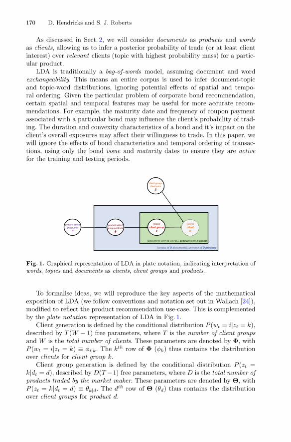
170 D. Hendricks and S. J. Roberts
As discussed in Sect. 2, we will consider documents as products and wordsas clients, allowing us to infer a posterior probability of trade (or at least clientinterest) over relevant clients (topic with highest probability mass) for a partic-ular product.
LDA is traditionally a bag-of-words model, assuming document and wordexchangeability. This means an entire corpus is used to infer document-topicand topic-word distributions, ignoring potential effects of spatial and tempo-ral ordering. Given the particular problem of corporate bond recommendation,certain spatial and temporal features may be useful for more accurate recom-mendations. For example, the maturity date and frequency of coupon paymentassociated with a particular bond may influence the client’s probability of trad-ing. The duration and convexity characteristics of a bond and it’s impact on theclient’s overall exposures may affect their willingness to trade. In this paper, wewill ignore the effects of bond characteristics and temporal ordering of transac-tions, using only the bond issue and maturity dates to ensure they are activefor the training and testing periods.
Fig. 1. Graphical representation of LDA in plate notation, indicating interpretation ofwords, topics and documents as clients, client groups and products.
To formalise ideas, we will reproduce the key aspects of the mathematicalexposition of LDA (we follow conventions and notation set out in Wallach [24]),modified to reflect the product recommendation use-case. This is complementedby the plate notation representation of LDA in Fig. 1.
Client generation is defined by the conditional distribution P (wt = i|zt = k),described by T (W − 1) free parameters, where T is the number of client groupsand W is the total number of clients. These parameters are denoted by Φ, withP (wt = i|zt = k) ≡ φi|k. The kth row of Φ (φk) thus contains the distributionover clients for client group k.
Client group generation is defined by the conditional distribution P (zt =k|dt = d), described by D(T −1) free parameters, where D is the total number ofproducts traded by the market maker. These parameters are denoted by Θ, withP (zt = k|dt = d) ≡ θk|d. The dth row of Θ (θd) thus contains the distributionover client groups for product d.

Optimal Client Recommendation for Market Makers 171
The joint probability of a set of products w and a set of associated latentgroups of interested clients z is
P (w, z|Φ,Θ) =∏
i
∏
k
∏
d
φNi|ki|k θ
Nk|dk|d , (2)
where Ni|k is the number of times client i has been generated by client group k,and Nk|d is the number of times client group k has been interested in product d.
As in Blei et al. [6], we assume a Dirichlet prior over Φ and Θ, i.e.
P (Φ|βm) =∏
k
Dirichlet(φk|βm) (3)
andP (Θ|αn) =
∏
d
Dirichlet(θd|αn). (4)
Combining these priors with Eq. 2 and integrating over Φ and Θ yields theprobability of the set of products given hyperparameters αn and βm:
P (w|αn, βm) =∑
z
( ∏
k
∏i Γ (Ni|k + βmi)Γ (Nk) + β
Γ (β)∏i Γ (βmi)
∏
d
∏k Γ (Nk|d + αnk)
Γ (Nd + α)Γ (α)∏
k Γ (αnk)
). (5)
In Eq. 5, Nk is the total number of times client group k occurs in z and Nd is thenumber of clients interested in product d. This posterior is intractable for exactinference, but a number of approximation schemes have been developed, notablyMarkov Chain Monte Carlo (MCMC) [15] and variational approximation [13,14].
For our study, we made use of the scikit-learn [20] open-source Python library,which includes an implementation of the online variational Bayes algorithm forLDA, described in Hoffman et al. [13,14]. They make use of a simpler, tractabledistribution to approximate Eq. 5, optimising the associated variational parame-ters to maximise the Evidence Lower Bound (ELBO), and hence minimising theKullback-Leibler (KL) divergence between the approximating distribution andthe true posterior.
4 Baseline Models for Comparison
1. Empirical Term-Frequency (ETF): We can use the normalised product-clientterm-frequency matrix discussed in Sect. 2.1 to construct an empirical prob-ability distribution over clients for each product. This encodes the historicalintensities of client interest, without exploiting any latent structure.
2. Non-negative Matrix Factorisation (NMF): NMF aims to discover latentstructure in a given non-negative matrix by using the product of two low-rank non-negative matrices as an approximation to the original, and min-imising the distance of the reconstruction to the original, measured by the
172 D. Hendricks and S. J. Roberts
Frobenius norm [18]. Applied to our problem, for a specified number of clientgroups, NMF can be used to reveal an unnormalised probability distributionover client groups for each product, and distribution over clients for eachclient group, from a given term-frequency matrix. These probabilities can benormalised for comparison with other models.
5 Evaluating Recommendation Efficacy
Recommender systems are usually evaluated in terms of their predictive accu-racy, but the appropriate metrics should be chosen to reflect success in thespecific application [22]. The data we have for inference and testing purposes isframed in terms of positive interest, viz. the presence of a record indicates a clientwas interest in the associated product, and the absence of a record indicates nointerest. In addition, we are interested in capturing the accuracy of a “top N”client list, as opposed to a binary classifier. In terms of the standard confusionmatrix metrics, we will thus focus on true and false positive results, however wehave implemented a nuanced interpretation based on our application:
– Cumulative True Positives (CTP): A client recommendation for a particu-lar product is classified as a True Positive (TP) if the recommended clientmatches the actual client for that product on the testing day. The total num-ber of TPs for a testing day is thus the total number of correctly matchedrecommendations. Given our use-case, where the N best (ranked) recommen-dations are sampled, we compute the cumulative TPs as the number of TPscaptured within the first x recommendations, x = 1, ..., N . More formally, theCTP for product j captured within the first x recommendations is given by
CTPxj =
x∑
i=1
I(wij=w∗
j ), (6)
where wij is the ith recommended client for product j and w∗
j is the actualclient who traded product j.
– Relevant False Positives (RFP): A client recommendation is classified as aRelevant False Positive (RFP) if is does not match the actual client for thatproduct on that day, but the recommended client traded another productinstead. The rationale here is that the model captures the property of gen-eral client trading interest, so may be useful for the sales traders to discusspossibilities with the client, even though the model has matched the client tothe incorrect product. These are measured at the first recommendation level(x = 1). For product j,
RFPj = I((w1
j �=w∗j )∩(w1
j∈{w∗k}k �=j)
). (7)
– Irrelevant False Positives (IFP): A client recommendation is classified asan Irrelevant False Positive (IFP) if is does not match the actual client for
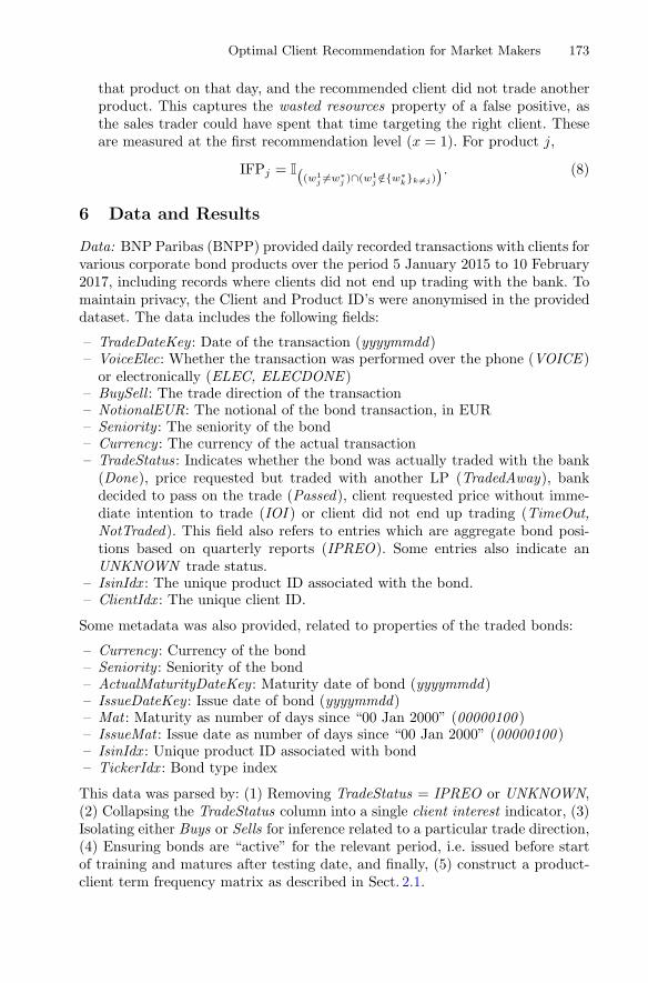
Optimal Client Recommendation for Market Makers 173
that product on that day, and the recommended client did not trade anotherproduct. This captures the wasted resources property of a false positive, asthe sales trader could have spent that time targeting the right client. Theseare measured at the first recommendation level (x = 1). For product j,
IFPj = I((w1
j �=w∗j )∩(w1
j /∈{w∗k}k �=j)
). (8)
6 Data and Results
Data: BNP Paribas (BNPP) provided daily recorded transactions with clients forvarious corporate bond products over the period 5 January 2015 to 10 February2017, including records where clients did not end up trading with the bank. Tomaintain privacy, the Client and Product ID’s were anonymised in the provideddataset. The data includes the following fields:
– TradeDateKey : Date of the transaction (yyyymmdd)– VoiceElec: Whether the transaction was performed over the phone (VOICE )
or electronically (ELEC, ELECDONE )– BuySell : The trade direction of the transaction– NotionalEUR: The notional of the bond transaction, in EUR– Seniority : The seniority of the bond– Currency : The currency of the actual transaction– TradeStatus: Indicates whether the bond was actually traded with the bank
(Done), price requested but traded with another LP (TradedAway), bankdecided to pass on the trade (Passed), client requested price without imme-diate intention to trade (IOI ) or client did not end up trading (TimeOut,NotTraded). This field also refers to entries which are aggregate bond posi-tions based on quarterly reports (IPREO). Some entries also indicate anUNKNOWN trade status.
– IsinIdx : The unique product ID associated with the bond.– ClientIdx : The unique client ID.
Some metadata was also provided, related to properties of the traded bonds:
– Currency : Currency of the bond– Seniority : Seniority of the bond– ActualMaturityDateKey : Maturity date of bond (yyyymmdd)– IssueDateKey : Issue date of bond (yyyymmdd)– Mat : Maturity as number of days since “00 Jan 2000” (00000100 )– IssueMat : Issue date as number of days since “00 Jan 2000” (00000100 )– IsinIdx : Unique product ID associated with bond– TickerIdx : Bond type index
This data was parsed by: (1) Removing TradeStatus = IPREO or UNKNOWN,(2) Collapsing the TradeStatus column into a single client interest indicator, (3)Isolating either Buys or Sells for inference related to a particular trade direction,(4) Ensuring bonds are “active” for the relevant period, i.e. issued before startof training and matures after testing date, and finally, (5) construct a product-client term frequency matrix as described in Sect. 2.1.
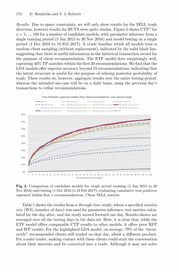
174 D. Hendricks and S. J. Roberts
Results: Due to space constraints, we will only show results for the SELL tradedirection, however results for BUYS were quite similar. Figure 2 shows CTPx forx = 1, ..., 100 for a number of candidate models, with parameter inference from asingle training period (5 Jan 2015 to 30 Nov 2016) and model testing on a singleperiod (1 Dec 2016 to 10 Feb 2017). A crude baseline which all models beat israndom client sampling (without replacement), indicated by the solid black line,suggesting that there is useful information in the historical transaction record forthe purpose of client recommendation. The ETF model does surprisingly well,capturing 40% TP matches within the first 20 recommendations. We find that theLDA models offer superior accuracy beyond 10 recommendations, indicating thatthe latent structure is useful for the purpose of refining posterior probability oftrade. These results do, however, aggregate results over the entire testing period,whereas the intended use-case will be on a daily basis, using the previous day’stransactions to refine recommendations.
Fig. 2. Comparison of candidate models for single period training (5 Jan 2015 to 30Nov 2016) and testing (1 Dec 2016 to 10 Feb 2017), evaluating cumulative true positivescaptured within first x recommendations. Client SELL interest.
Table 1 shows the results from a through-time study, where a specified windowsize (WS) (number of days) was used for parameter inference, test metrics calcu-lated for the day after, and the study moved forward one day. Results shown areaveraged over all the testing days in the data set. Here, it is clear that, while theETF model offers comparable CTP results to other models, it offers poor RFPand IFP results. For the highlighted LDA model, on average, 79% of the “incor-rectly” recommended clients still traded on that day, albeit a different product.For a sales trader, making contact with these clients could start the conversationabout their interests and be converted into a trade. Although it may not solve
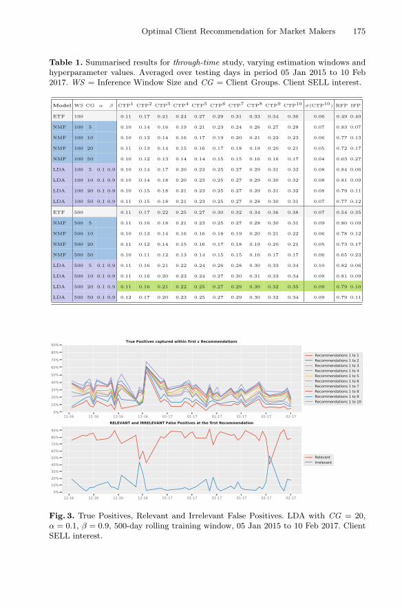
Optimal Client Recommendation for Market Makers 175
Table 1. Summarised results for through-time study, varying estimation windows andhyperparameter values. Averaged over testing days in period 05 Jan 2015 to 10 Feb2017. WS = Inference Window Size and CG = Client Groups. Client SELL interest.
Model WS CG α β CTP1 CTP2 CTP3 CTP4 CTP5 CTP6 CTP7 CTP8 CTP9 CTP10 σ(CTP10) RFP IFP
ETF 100 0.11 0.17 0.21 0.24 0.27 0.29 0.31 0.33 0.34 0.36 0.06 0.49 0.40
NMF 100 5 0.10 0.14 0.16 0.19 0.21 0.23 0.24 0.26 0.27 0.28 0.07 0.83 0.07
NMF 100 10 0.10 0.13 0.14 0.16 0.17 0.19 0.20 0.21 0.22 0.23 0.06 0.77 0.13
NMF 100 20 0.11 0.13 0.14 0.15 0.16 0.17 0.18 0.19 0.20 0.21 0.05 0.72 0.17
NMF 100 50 0.10 0.12 0.13 0.14 0.14 0.15 0.15 0.16 0.16 0.17 0.04 0.63 0.27
LDA 100 5 0.1 0.9 0.10 0.14 0.17 0.20 0.23 0.25 0.27 0.29 0.31 0.32 0.08 0.84 0.06
LDA 100 10 0.1 0.9 0.10 0.14 0.18 0.20 0.23 0.25 0.27 0.29 0.30 0.32 0.08 0.81 0.09
LDA 100 20 0.1 0.9 0.10 0.15 0.18 0.21 0.23 0.25 0.27 0.29 0.31 0.32 0.08 0.79 0.11
LDA 100 50 0.1 0.9 0.11 0.15 0.18 0.21 0.23 0.25 0.27 0.28 0.30 0.31 0.07 0.77 0.12
ETF 500 0.11 0.17 0.22 0.25 0.27 0.30 0.32 0.34 0.36 0.38 0.07 0.54 0.35
NMF 500 5 0.11 0.16 0.18 0.21 0.23 0.25 0.27 0.28 0.30 0.31 0.09 0.80 0.09
NMF 500 10 0.10 0.13 0.14 0.16 0.16 0.18 0.19 0.20 0.21 0.22 0.06 0.78 0.12
NMF 500 20 0.11 0.12 0.14 0.15 0.16 0.17 0.18 0.19 0.20 0.21 0.05 0.73 0.17
NMF 500 50 0.10 0.11 0.12 0.13 0.14 0.15 0.15 0.16 0.17 0.17 0.06 0.65 0.23
LDA 500 5 0.1 0.9 0.11 0.16 0.21 0.22 0.24 0.26 0.28 0.30 0.33 0.34 0.10 0.82 0.06
LDA 500 10 0.1 0.9 0.11 0.16 0.20 0.23 0.24 0.27 0.30 0.31 0.33 0.34 0.09 0.81 0.09
LDA 500 20 0.1 0.9 0.11 0.16 0.21 0.22 0.25 0.27 0.29 0.30 0.32 0.35 0.09 0.79 0.10
LDA 500 50 0.1 0.9 0.12 0.17 0.20 0.23 0.25 0.27 0.29 0.30 0.32 0.34 0.09 0.79 0.11
Fig. 3. True Positives, Relevant and Irrelevant False Positives. LDA with CG = 20,α = 0.1, β = 0.9, 500-day rolling training window, 05 Jan 2015 to 10 Feb 2017. ClientSELL interest.
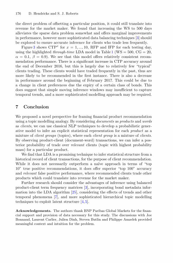
176 D. Hendricks and S. J. Roberts
the direct problem of offsetting a particular position, it could still translate intorevenue for the market maker. We found that increasing the WS to 500 daysalleviates the sparse data problem somewhat and offers marginal improvementsin performance, however more sophisticated data balancing techniques [3] shouldbe explored to ensure accurate inference for clients who trade less frequently.
Figure 3 shows CTPx for x = 1, ..., 10, RFP and IFP for each testing day,using the highlighted through-time LDA model in Table 1 (WS = 500, CG = 20,α = 0.1, β = 0.9). We see that this model offers relatively consistent recom-mendation performance. There is a significant increase in CTP accuracy aroundthe end of December 2016, but this is largely due to relatively few “typical”clients trading. These clients would have traded frequently in the past, thus aremore likely to be recommended in the first instance. There is also a decreasein performance around the beginning of February 2017. This could be due toa change in client preferences due the expiry of a certain class of bonds. Thisdoes suggest that simple moving inference windows may insufficient to capturetemporal trends, and a more sophisticated modelling approach may be required.
7 Conclusion
We proposed a novel perspective for framing financial product recommendationusing a topic modelling analogy. By considering documents as products and wordsas clients, we can use classical NLP techniques to develop a probabilistic gener-ative model to infer an explicit statistical representation for each product as amixture of client groups (topics), where each client group is a mixture of clients.By observing product-client (document-word) transactions, we can infer a pos-terior probability of trade over relevant clients (topic with highest probabilitymass) for a particular product.
We find that LDA is a promising technique to infer statistical structure from ahistorical record of client transactions, for the purpose of client recommendation.While it does not necessarily outperform a naıve approach in terms of “top10” true positive recommendations, it does offer superior “top 100” accuracyand relevant false positive performance, where recommended clients trade otherproducts which could translate into revenue for the market maker.
Further research should consider the advantages of inference using balancedproduct-client term frequency matrices [3], incorporating bond metadata infor-mation into the LDA algorithm [25], considering the effects of trends and othertemporal phenomena [7], and more sophisticated hierarchical topic modellingtechniques to exploit latent structure [4,5].
Acknowledgements. The authors thank BNP Paribas Global Markets for the finan-cial support and provision of data necessary for this study. The discussions with JoeBonnaud, Laurent Carlier, Julien Dinh, Steven Butlin and Philippe Amzelek providedmeaningful context and intuition for the problem.

Optimal Client Recommendation for Market Makers 177
References
1. Amihud, Y., Mendelson, H.: Asset pricing and the bid-ask spread. J. Financ. Econ.17(2), 223–249 (1986)
2. Avellaneda, M., Stoikov, S.: High-frequency trading in a limit order book. Quant.Finan. 8(3), 217–224 (2016)
3. Batista, G.E., Prati, R.C., Monard, M.C.: A study of the behavior of several meth-ods for balancing machine learning training data. ACM SIGKDD Explor. Newslett.6(1), 20–29 (2004)
4. Blei, D.M., Griffiths, T.L., Jordan, M.I.: The nested Chinese Restaurant Processand Bayesian nonparametric inference of topic hierarchies. J. ACM (JACM) 57(2),7 (2010)
5. Blei, D.M., Griffiths, T.L., Jordan, M.I., Tenenbaum, J.B.: Hierarchical topic mod-els and the nested Chinese Restaurant Process. In: Advances in Neural InformationProcessing (2004)
6. Blei, D.M., Ng, A.Y., Jordan, M.I.: Latent dirichlet allocation. J. Mach. Learn.Res. 3, 993–1022 (2003)
7. Bolelli, L., Ertekin, S., Giles, C.L.: Topic and trend detection in text collec-tions using latent dirichlet allocation. In: Boughanem, M., Berrut, C., Mothe, J.,Soule-Dupuy, C. (eds.) ECIR 2009. LNCS, vol. 5478, pp. 776–780. Springer,Heidelberg (2009). https://doi.org/10.1007/978-3-642-00958-7 84
8. Das, S., Magdon-Ismail, M.: Adapting to a market shock: optimal sequentialmarket-making. In: Advances in Neural Information Processing Systems (2009)
9. Duffie, D.: Market making under the proposed volcker rule. Rock Center for Cor-porate Governance at Stanford University Working Paper No. 106 (2012)
10. Elton, E.J., Gruber, M.J., Agrawal, D., Mann, C.: Explaining the rate spread oncorporate bonds. J. Finan. 56(1), 247–277 (2001)
11. Ghoshal, S., Roberts, S.: Optimal FX market making under inventory risk andadverse selection constraints. Working paper (2016)
12. Gueant, O.: Optimal market making (2017). arXiv:1605.01862 [q-fin.TR]13. Hoffman, M., Bach, F.R., Blei, D.M.: Online learning for Latent Dirichlet Alloca-
tion. In: Advances in Neural Information Processing (2010)14. Hoffman, M., Blei, D.M., Wang, C., Paisley, J.W.: Stochastic variational inference.
J. Mach. Learn. Res. 14(1), 1303–1347 (2013)15. Jordan, M.I.: Learning in Graphical Models, vol. 89. Springer, Berlin (1998)16. Kaal, W.A.: Global Encyclopedia of Public Administration, Public Policy, and
Governance: Dodd-Frank Act. Springer (2016)17. Kim, I., Ramaswamy, K., Sundaresan, S.: The Valuation of Corporate Fixed
Income Securities. Columbia University, Manuscript (1988)18. Lee, D.D., Seung, H.S.: Learning the parts of objects by non-negative matrix fac-
torization. Nature 401, 788–791 (1999)19. MacKay, D.J.C., Bauman Peto, L.C.: A hierarchical Dirichlet language model. Nat.
Lang. Eng. 1(3), 289–308 (1995)20. Pedregosa, F., Varoquaux, G., Gramfort, A., Michel, V., Thirion, B., Grisel, O.,
Blondel, M., Prettenhofer, P., Weiss, R., Dubourg, V., et al.: Scikit-learn: machinelearning in python. J. Mach. Learn. Res. 12, 2825–2830 (2011)
21. Robertson, S.: Understanding inverse document frequency: on theoretical argu-ments for IDF. J. Documentation 60(5), 503–520 (2004)
22. Shani, G., Gunawardana, A.: Evaluating Recommendation Systems. RecommenderSystems Handbook. Springer, US (2011)

178 D. Hendricks and S. J. Roberts
23. Jones, K.S.: A statistical interpretation of term specificity and its application inretrieval. J. Documentation 28, 11–21 (1972)
24. Wallach, H.M.: Topic modeling: beyond bag-of-words. In: Proceedings of the 23rdInternational Conference on Machine Learning, pp. 977–984 (2006)
25. Wang, X., Grimson, E.: Spatial latent dirichlet allocation. In: Advances in NeuralInformation Processing Systems, pp. 1577–1584 (2008)
Predicting Self-reported Customer Satisfactionof Interactions with a Corporate Call Center
Joseph Bockhorst(B), Shi Yu, Luisa Polania, and Glenn Fung
Machine Learning Unit, Strategic Data & Analytics, American Family Insurance,6000 American Parkway, Madison, WI 53783, USA
Abstract. Timely identification of dissatisfied customers would providecorporations and other customer serving enterprises the opportunity totake meaningful interventions. This work describes a fully operationalsystem we have developed at a large US insurance company for predict-ing customer satisfaction following all incoming phone calls at our callcenter. To capture call relevant information, we integrate signals frommultiple heterogeneous data sources including: speech-to-text transcrip-tions of calls, call metadata (duration, waiting time, etc.), customer pro-files and insurance policy information. Because of its ordinal, subjective,and often highly-skewed nature, self-reported survey scores presents sev-eral modeling challenges. To deal with these issues we introduce a novelmodeling workflow: First, a ranking model is trained on the customercall data fusion. Then, a convolutional fitting function is optimized tomap the ranking scores to actual survey satisfaction scores. This app-roach produces more accurate predictions than standard regression andclassification approaches that directly fit the survey scores with call data,and can be easily generalized to other customer satisfaction predictionproblems. Source code and data are available at https://github.com/cyberyu/ecml2017.
1 Introduction
In a competitive customer-driven landscape where businesses are constantly com-peting to attract and retain customers; customer satisfaction is one of the topdifferentiators. While digitization and other forces continue to increase consumerchoice, understanding and improving customer satisfaction are often core ele-ments of the business strategy of modern companies. It enables service providersto unveil timely opportunities to take meaningful interventions to improve cus-tomer experience and to train customer representatives (CR) in an optimal way.
In order to measure the effectiveness of a CR during a phone interaction witha customer, generally a customer survey is taken shortly after the call takes place.However, due to survey expense, typically only a small percentage of calls aremeasured. When CR performance is calculated from a small sample of surveysperformance scores have high variability and there is potential misrepresentationof CR performance.c© Springer International Publishing AG 2017Y. Altun et al. (Eds.): ECML PKDD 2017, Part III, LNAI 10536, pp. 179–190, 2017.https://doi.org/10.1007/978-3-319-71273-4_15

180 J. Bockhorst et al.
The focus of this work is to describe the design and implementation of adeployed machine-learning-based system used to automatically predict customersatisfaction following phone calls. Our discovery and system design process canbe divided into four stages:
1. Extraction, processing and linking of raw data: Raw data is collectedand linked from four primary sources: call logs, historical survey scores, cus-tomer and policy databases, and call transcription and related content derivedfrom audio recordings.
2. Feature engineering: Call data is processed to create informative features.3. Model design and creation: In this stage we focus on the design and
creating of the customer satisfaction predictive models.4. Aggregation of model predictions to the group level: At the last stage,
we aggregate individual model predictions to the group level (by call queue,by CR, in a given period of time, etc.). We also provide estimated bounds forthe group average predictions.
2 Related Work
Research studies on emotion recognition using human-human real-life corpusextracted from call center calls are limited. In [15], a system for emotion recog-nition in the call center domain, using lexical and paralinguistic cues, is proposed.The goal was to classify parts of dialogs into three emotional states. Trainingand testing was performed on a corpus of 18 h of real dialogs between agent andcustomer, collected in a service of complaints. A similar work [2], also proposes toclassify call center calls between three emotional states, namely, anger, positiveand neutral. The authors used classical descriptors, such as zero crossing rateand Mel-frequency cepstral coefficients, and support vector machines as the clas-sifier. They used service complaints and medical emergency conversations fromcall centers, and adopted a cross-corpus methodology for the experiments, mean-ing that they use one corpus as training set and another corpus as test set. Theyattained a classification accuracy between 40% to 50% for all the experiments.
Park and Gates [10] developed a method to automatically measure customersatisfaction by analyzing call transcripts in near real-time. They identified sev-eral linguistics and prosodic features that are highly correlated with behavioralaspects of the speakers and built machine learning models that predict thedegree of customer satisfaction in a scale from 1 to 5 with an accuracy of 66%.Sun et al. [13] adopted a different approach, based on fusion techniques, to pre-dict the user emotional state from dialogs extracted from a Chinese Mobile callcenter corpus. They implemented a statistical model fusion to alleviate the dataimbalance problem and combined n-gram features, sentiment word features anddomain-specific words features for classification.
Recently, convolutional neural networks have been used on raw audio signalsto automatically learn meaningful features that lead to successful prediction ofself-reported customer satisfaction from call center conversations in Spanish [12].This approach starts by pretraining a network on debates from French TV shows

Predicting Self-reported Customer Satisfaction of Interactions 181
with the goal of detecting salient information in raw speech that correlates withemotion. Then, the last layers of the network are finetuned with more than 18000conversations from several call centers. The CNN-based system achieved compa-rable performance to the systems based on traditional hand-designed features.
There are many machine learning problems, referred to as ordinal rankingproblems, where the goal is to classify patterns using a categorical scale whichshows a natural order between labels, but not a meaningful numeric differencebetween them. For example, emotion recognition in the call center domain usu-ally involves rating based on an ordinal scale. Indeed, psychometric studies showthat human ratings of emotion do not follow an absolute scale [8,9]. Ordinalranking is fundamentally different from nominal classification techniques in thatorder is relevant and the labels are not treated as independent output categories.The ordinal ranking problems may not be optimally addressed by the standardregression either since the absolute difference of output values is nearly mean-ingless and only their relative order matters [3].
There are several algorithms which specifically benefit from the orderinginformation and yield better performance than nominal classification and regres-sion approaches. For example, Herbrich et al. [5] proposed a support vec-tor machines approach based on comparing training examples in a pairwisemanner. A constraint classification approach that works with binary classifiersand is based on the pairwise comparison framework was proposed by Har-Peledet al. [4]. Crammer and Singer [1] developed an ordinal ranking algorithm basedon the online perceptron algorithm with multiple thresholds.
Some areas where ordinal ranking problems are found include medicalresearch [11], brain computer interface [17], credit rating [7], facial beauty assess-ment [16], image classification [14], and more. All these works are examples ofapplications of ordinal ranking models, where exploiting ordering informationimproves their performance with respect to their nominal counterparts.
3 Overview of the Proposed System
Our main goal is to develop a model to predict satisfaction scores for all incomingcustomer calls in order to (i) take meaningful timely interventions to improvecustomer experience and (ii) obtain a robust understanding on how care centerperformance and training can be enhanced, ultimately for our customer’s benefit.
Our company recently adopted a system which automatically transcribesphone calls to text. The transcriptions generated by this system are key for ourdeployed system. The company customer care center monitors customer satisfac-tion by offering surveys conducted by a third party vendor to 10% of incomingcalls. Each care center CR has around five surveys completed per month, whichis only about 0.5–1% of all assigned calls. There are four topics measured bythe survey: (a) If the customer felt “valued” during the call; (b) If the issue wasresolved; (c) How polite the CR was, and (d) How clearly the CR communi-cated during the call. Scores range form 1 to 10 (1 lowest, 10 highest) and thefour scores are averaged into an additional variable called RSI (RepresentativeSatisfaction Index). In this paper we focus on predicting the RSI.

182 J. Bockhorst et al.
Several difficulties, in terms of modeling, are discovered after a quick initialinspection of the training data:
– The customer satisfaction scores (RSI) are highly biased towards the highestscore (10), while calls with scores lower than 8 are less than 4%. This highlyskewed distribution makes building a predictive model more complex.
– Survey scores are customer responses, thus are subjective, qualitative statesheavily impacted by personal preferences.
– The measurement scale of survey scores is ordinal; one cannot say, for exam-ple, that a score of 10 indicates double satisfaction as a score of 5. Most, ifnot all, standard regression techniques implicitly assume an interval or ratioscale.
Figure 1 displays an overview of the deployed system. The system workflowcan be summarized by the following steps:
1. After a call ends, a transcript of the call is automatically produced by aspeech-to-text system developed by Voci (vocitec.com).
2. Calls are partitioned into temporal segments and non-text features are engi-neered. The rationale of temporal segmentation is that certain events aremore relevant depending of when they occur in the call. For example: detect-ing negative sentiment trends in the first quarter of the call but positive atthe end may lead to a higher satisfaction score than when the opposite istrue.
3. Textual features are constructed and merged with non-text features. Thefused feature vectors are used as input features for the models described inthe next step.
4. Ranking model scoring. The ranking model is trained by sampling orderedpairs based on satisfaction scores.
Fig. 1. Overview of the deployed system
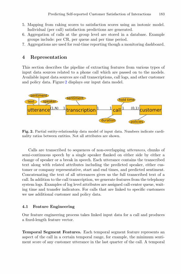
Predicting Self-reported Customer Satisfaction of Interactions 183
5. Mapping from raking scores to satisfaction scores using an isotonic model.Individual (per call) satisfaction predictions are generated.
6. Aggregation of calls at the group level are stored in a database. Examplegroups include: per CR, per queue and per time period.
7. Aggregations are used for real-time reporting though a monitoring dashboard.
4 Representation
This section describes the pipeline of extracting features from various types ofinput data sources related to a phone call which are passed on to the models.Available input data sources are call transcriptions, call logs, and other customerand policy data. Figure 2 displays our input data model.
Fig. 2. Partial entity-relationship data model of input data. Numbers indicate cardi-nality ratios between entities. Not all attributes are shown.
Calls are transcribed to sequences of non-overlapping utterances, chunks ofsemi-continuous speech by a single speaker flanked on either side by either achange of speaker or a break in speech. Each utterance contains the transcribedtext along with related attributes including the predicted speaker, either cus-tomer or company representative, start and end times, and predicted sentiment.Concatenating the text of all utterances gives us the full transcribed text of acall. In addition to the call transcription, we generate features from the telephonysystem logs. Examples of log level attributes are assigned call-center queue, wait-ing time and transfer indicators. For calls that are linked to specific customerswe use additional customer and policy data.
4.1 Feature Engineering
Our feature engineering process takes linked input data for a call and producesa fixed-length feature vector.
Temporal Segment Features. Each temporal segment feature represents anaspect of the call in a certain temporal range, for example, the minimum senti-ment score of any customer utterance in the last quarter of the call. A temporal

184 J. Bockhorst et al.
Table 1. A temporal segment feature is created for each of the 300 combinations(5 × 3 × 4 × 5) of component values.
Component Possible values
Utterance function negSent(), negCount(), duration(), consNeg(), sentScore()
Speaker representative, customer, either
Aggregate function min(), max(), mean(), std()
Temporal range [0.0, 0.25), [0.25, 0.5), [0.5, 0.75), [0.75, 1.0], [0.9, 1.0]
segment feature is defined by (i) a numerical utterance function1, (ii) a speaker,(iii) an aggregate function and, (iv) a temporal range (see Table 1).
Temporal Segment Text-Features. The text of each transcribed customercall can also be viewed as a linear sequence of temporal elements (words) thuscan be decomposed into temporal textual segmentations. In fact, each customercall consists of several natural temporal segmentations, which usually starts withgreetings, then customer personal information authentication, next followed bycustomer’s narrations of problems or requests, and then responses and resolu-tions provided by the representative, and finishes by ending courtesies of bothparties. To predict customer satisfaction, we assume that late segmentations ofa call (i.e., problem explanations, resolutions) are more informative than earlyparts (i.e., greetings, authentication), therefore we create separate textual modelsby decomposing the transcribed text of a call into different temporal segments.
We denote D as the corpus of transcribed text of all calls, where di ∈ D,i = 1...N is a document of transcribed text of the i-th call. Each di is composedof a sequence of words wi,j , j = 1...Mi where Mi is the total number of wordsin di. And we further decompose all the words in a document into four sub-documents qi1, qi2, qi3, qi4, where
qi1 = {wi,1, ..., wi,s1},
qi2 = {wi,s1+1, ..., wi,s2},
qi3 = {wi,s2+1, ..., wi,s3},
qi4 = {wi,s3+1, ..., wi,Mi}.
Since each call has different lengths, and we haven’t applied any method toautomatically segment a call according to the content, we simply set s1, s2, s3respectively to the rounded integers of Mi
4 , 2Mi
4 , 3Mi
4 , thus gives us four even
1 negSent() is an indicator that is 1 if the utterance sentiment label is Negative,negCount() is the number of Negative or Mostly Negative sentiment phrases in theutterance, duration() is the length of the utterance in seconds, consNeg() is an indi-cator that is 1 if the current and previous utterance have negative sentiment, andsentScore() maps utterance sentiment labels (Negative, Mostly Negative, Neutral,Mostly Positive, Positive) to numerical scores (−1,−0.5, 0, 0.5, 1).
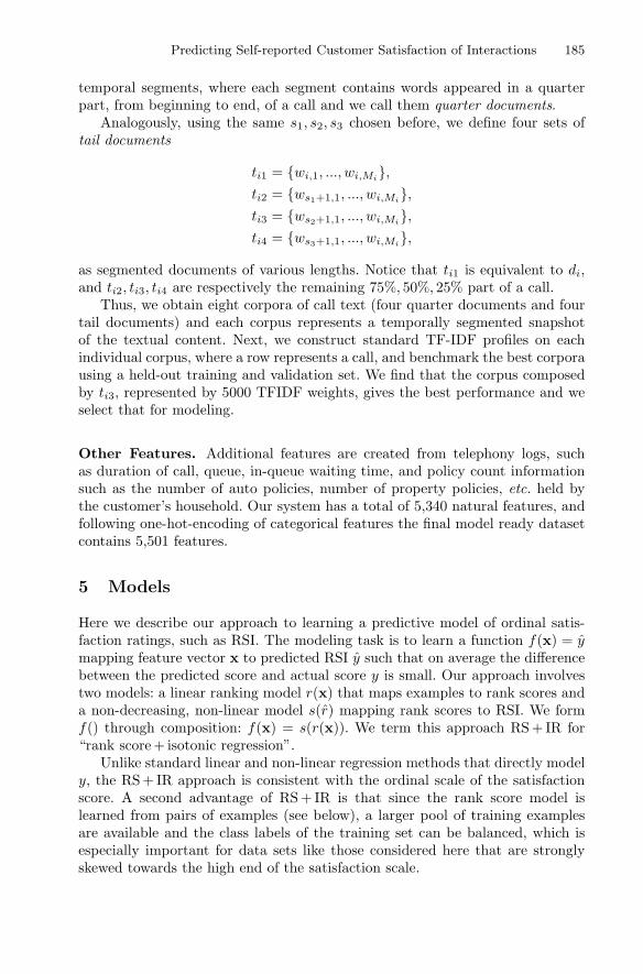
Predicting Self-reported Customer Satisfaction of Interactions 185
temporal segments, where each segment contains words appeared in a quarterpart, from beginning to end, of a call and we call them quarter documents.
Analogously, using the same s1, s2, s3 chosen before, we define four sets oftail documents
ti1 = {wi,1, ..., wi,Mi},
ti2 = {ws1+1,1, ..., wi,Mi},
ti3 = {ws2+1,1, ..., wi,Mi},
ti4 = {ws3+1,1, ..., wi,Mi},
as segmented documents of various lengths. Notice that ti1 is equivalent to di,and ti2, ti3, ti4 are respectively the remaining 75%, 50%, 25% part of a call.
Thus, we obtain eight corpora of call text (four quarter documents and fourtail documents) and each corpus represents a temporally segmented snapshotof the textual content. Next, we construct standard TF-IDF profiles on eachindividual corpus, where a row represents a call, and benchmark the best corporausing a held-out training and validation set. We find that the corpus composedby ti3, represented by 5000 TFIDF weights, gives the best performance and weselect that for modeling.
Other Features. Additional features are created from telephony logs, suchas duration of call, queue, in-queue waiting time, and policy count informationsuch as the number of auto policies, number of property policies, etc. held bythe customer’s household. Our system has a total of 5,340 natural features, andfollowing one-hot-encoding of categorical features the final model ready datasetcontains 5,501 features.
5 Models
Here we describe our approach to learning a predictive model of ordinal satis-faction ratings, such as RSI. The modeling task is to learn a function f(x) = ymapping feature vector x to predicted RSI y such that on average the differencebetween the predicted score and actual score y is small. Our approach involvestwo models: a linear ranking model r(x) that maps examples to rank scores anda non-decreasing, non-linear model s(r) mapping rank scores to RSI. We formf() through composition: f(x) = s(r(x)). We term this approach RS + IR for“rank score + isotonic regression”.
Unlike standard linear and non-linear regression methods that directly modely, the RS + IR approach is consistent with the ordinal scale of the satisfactionscore. A second advantage of RS + IR is that since the rank score model islearned from pairs of examples (see below), a larger pool of training examplesare available and the class labels of the training set can be balanced, which isespecially important for data sets like those considered here that are stronglyskewed towards the high end of the satisfaction scale.

186 J. Bockhorst et al.
Rank Score Model. We learn a model to rank examples by RSI using thepairwise transform [6]. The pairwise transform induces a rank score function r(x)by learning a linear binary classifier from an auxiliary training set of examples(u, v) that are formed from pairs of examples (xi, yi), (xj, yj) in the originalordinal training set that have different satisfaction scores2.
The features of the auxiliary examples are the component-wise differencebetween the original examples, uij = xi−xj. The binary class value vij indicateswhether or not example i has a higher satisfaction than example j: vij is +1 ifyi > yj and −1 if yi < yj . The linear binary classifier r(u), which is learnedfrom the auxiliary training set to predict which of two examples has a highersatisfaction score, is subsequently used as a rank score function r(x). That r() canbe used as a ranking function follows from its linearity r(xi−xj) = r(xi)−r(xj)and by noticing that r(xi) > r(xj) is consistent with the prediction that yi islarger than yj .
Rank Score to Satisfaction. The second sub-model s(r) is one-dimensional,non-decreasing function mapping rank scores to satisfaction scores. After learn-ing the rank score model r() we calculate the rank score of all examples in theoriginal training set, order examples by their rank scores and smooth the result-ing sequence of satisfaction scores. We then fit an isotonic regression model usingtraining examples sampled uniformly from the smoothed function.
6 Results
In this section we describe the results of experiments conducted on a data set of8,726 incoming phone calls from between March 23, 2015 and Dec 29, 2015 forwhich we have customer satisfaction survey results. We randomly selected 75%(6,108) for the training set and the remainder served as our test set.
6.1 Individual Predictions
To assess the value of our “rank score + isotonic regression” (RS + IR) app-roach to predicting phone call representative satisfaction index (RSI) scores wecompared it with three standard regression methods (ridge regression, Lassoand random forest regression) and one classification method, linear support vec-tor machine3. Ridge regression and Lasso are both penalized linear regressionmethods, but use different loss functions: L2 for ridge and L1 for lasso. Ran-dom forest regression is a non-linear approach that trains different ensembles of2 All the auxiliary examples may not be needed. We have found that while there are
over 10 million auxiliary examples that can be formed from our training set, the rankscore model is well converged when trained with 10,000 examples. We experimentedwith various techniques for sampling the auxiliary examples (biased for large RSIdifference, small RSI difference, etc.), and found that simple uniform sampling worksbest.
3 All comparison models trained using the scikit-learn Python package.
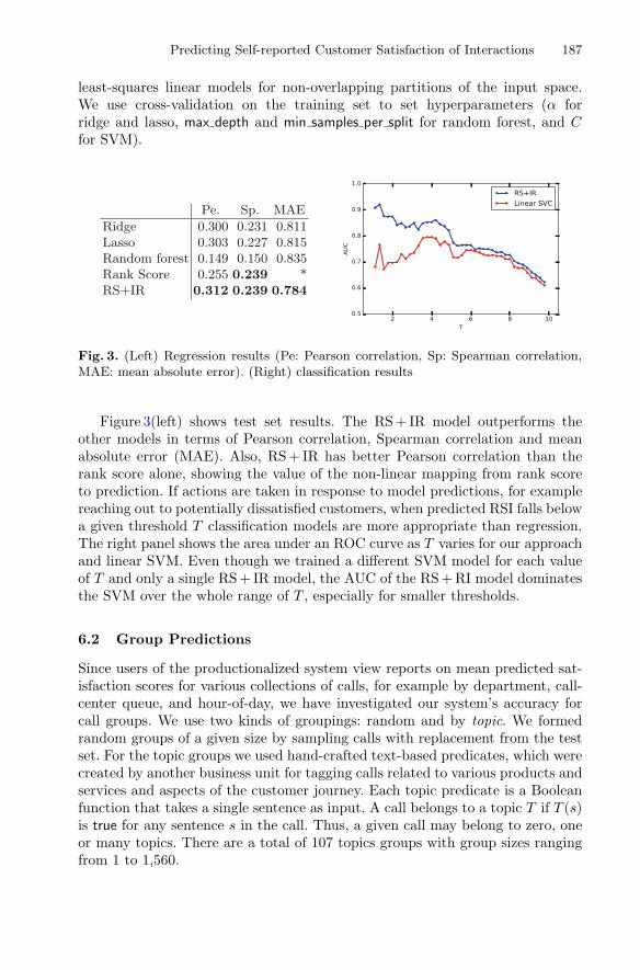
Predicting Self-reported Customer Satisfaction of Interactions 187
least-squares linear models for non-overlapping partitions of the input space.We use cross-validation on the training set to set hyperparameters (α forridge and lasso, max depth and min samples per split for random forest, and Cfor SVM).
Pe. Sp. MAERidge 0.300 0.231 0.811Lasso 0.303 0.227 0.815Random forest 0.149 0.150 0.835Rank Score 0.255 0.239 *RS+IR 0.312 0.239 0.784
Fig. 3. (Left) Regression results (Pe: Pearson correlation, Sp: Spearman correlation,MAE: mean absolute error). (Right) classification results
Figure 3(left) shows test set results. The RS + IR model outperforms theother models in terms of Pearson correlation, Spearman correlation and meanabsolute error (MAE). Also, RS + IR has better Pearson correlation than therank score alone, showing the value of the non-linear mapping from rank scoreto prediction. If actions are taken in response to model predictions, for examplereaching out to potentially dissatisfied customers, when predicted RSI falls belowa given threshold T classification models are more appropriate than regression.The right panel shows the area under an ROC curve as T varies for our approachand linear SVM. Even though we trained a different SVM model for each valueof T and only a single RS + IR model, the AUC of the RS + RI model dominatesthe SVM over the whole range of T , especially for smaller thresholds.
6.2 Group Predictions
Since users of the productionalized system view reports on mean predicted sat-isfaction scores for various collections of calls, for example by department, call-center queue, and hour-of-day, we have investigated our system’s accuracy forcall groups. We use two kinds of groupings: random and by topic. We formedrandom groups of a given size by sampling calls with replacement from the testset. For the topic groups we used hand-crafted text-based predicates, which werecreated by another business unit for tagging calls related to various products andservices and aspects of the customer journey. Each topic predicate is a Booleanfunction that takes a single sentence as input. A call belongs to a topic T if T (s)is true for any sentence s in the call. Thus, a given call may belong to zero, oneor many topics. There are a total of 107 topics groups with group sizes rangingfrom 1 to 1,560.

188 J. Bockhorst et al.
(a) (b)
Fig. 4. (a) Dashed lines indicate 95% confidence band for randomly selected groups.Points are observed group errors of topics groups containing more than 50 calls. (b)Quantile/quantile plot of group errors for the topics groups.
We define the group error to be the difference between the mean of thepredicted scores for all calls in the group and the mean of the actual satisfactionscores. We form random groups with between 10 and 1,000 calls and for eachgroup size we formed 5,000 replicate random groups. The dashed blue lines inFig. 4(a) show 95% confidence bands for the group error of the random groups.That is, for a given group size the group error of 95% of groups of that size inour simulation fell between the bands. We can see from this figure that grouperror decreases with group size.
We use the bands of Fig. 4(a) to determine tolerance levels for deciding whento raise alarms due to differences between predicted and actual satisfactionscores. The points represent the errors of the topics groups. The errors for 45of the 48 topics groups (93.75%) with more than 50 calls fall between the 95%confidence bands. This provides evidence that the topic groups have similar errorprofiles to natural groupings by topic. Figure 4(b) shows the quantile/quantileplot for the group error of all 107 topics groups using the errors of random groupsof similar size to compute the observed percentile. As the points lie close to theideal diagonal line, we conclude that the error profiles of random groups andtopics group are similar.
Figure 5(a) shows the predicted and actual mean satisfaction for topics groupswith at least 50 calls. The area of each bubble is proportional to the numberof calls in the group, which ranges from a minimum of 50 to a maximum of1,560. There is a general agreement (Pearson correlation = 0.73) between thepredicted and actual group means. And in general, as with the random groups,larger groups have smaller within group errors. Figure 5(b) shows the predictedgroup mean with 95% confidence interval (dependent on the group size) and theactual group mean for these same 48 groups. Again, as this is a different view ofthe same data represented by the points of Fig. 4(a), we see that the confidencebounds determined by random group errors do an excellent job of describing thedistribution of errors in the topics groups.
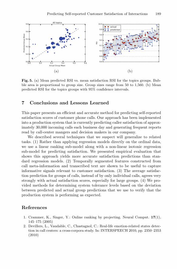
Predicting Self-reported Customer Satisfaction of Interactions 189
(a) (b)
Fig. 5. (a) Mean predicted RSI vs. mean satisfaction RSI for the topics groups. Bub-ble area is proportional to group size. Group sizes range from 50 to 1,560. (b) Meanpredicted RSI for the topics groups with 95% confidence intervals.
7 Conclusions and Lessons Learned
This paper presents an efficient and accurate method for predicting self-reportedsatisfaction scores of customer phone calls. Our approach has been implementedinto a production system that is currently predicting caller satisfaction of approx-imately 30,000 incoming calls each business day and generating frequent reportsread by call-center mangers and decision makers in our company.
We described several techniques that we suspect will generalize to relatedtasks. (1) Rather than applying regression models directly on the ordinal data,we use a linear ranking sub-model along with a non-linear isotonic regressionsub-model for predicting satisfaction. We presented empirical evaluation thatshows this approach yields more accurate satisfaction predictions than stan-dard regression models. (2) Temporally segmented features constructed fromcall meta-information and transcribed text are shown to be useful to captureinformative signals relevant to customer satisfaction. (3) The average satisfac-tion prediction for groups of calls, instead of by only individual calls, agrees verystrongly with actual satisfaction scores, especially for large groups. (4) We pro-vided methods for determining system tolerance levels based on the deviationbetween predicted and actual group predictions that we use to verify that theproduction system is performing as expected.
References
1. Crammer, K., Singer, Y.: Online ranking by projecting. Neural Comput. 17(1),145–175 (2005)
2. Devillers, L., Vaudable, C., Chastagnol, C.: Real-life emotion-related states detec-tion in call centers: a cross-corpora study. In: INTERSPEECH 2010, pp. 2350–2353(2010)
190 J. Bockhorst et al.
3. Gutierrez, P., Perez-Ortiz, M., Sanchez-Monedero, J., Fernandez-Navarro, F.,Hervas-Martinez, C.: Ordinal regression methods: survey and experimental study.IEEE Trans. Knowl. Data Eng. 28(1), 127–146 (2016)
4. Har-Peled, S., Roth, D., Zimak, D.: Constraint classification: a new approach tomulticlass classification. In: Cesa-Bianchi, N., Numao, M., Reischuk, R. (eds.) ALT2002. LNCS (LNAI), vol. 2533, pp. 365–379. Springer, Heidelberg (2002). https://doi.org/10.1007/3-540-36169-3 29
5. Herbrich, R., Graepel, T., Obermayer, K.: Large margin rank boundaries for ordi-nal regression. In: Advances in Neural Information Processing Systems, pp. 115–132(1999)
6. Herbrich, R., Graepel, T., Obermayer, K.: Support vector learning for ordinalregression. In: International Conference on Artificial Neural Networks, pp. 97–102(1999)
7. Kim, K., Ahn, H.: A corporate credit rating model using multiclass support vec-tor machines with an ordinal pairwise partitioning approach. Comput. Oper. Res.39(8), 1800–1811 (2012)
8. Metallinou, A., Narayanan, S.: Annotation and processing of continuous emotionalattributes: challenges and opportunities. In: IEEE International Conference andWorkshops on Automatic Face and Gesture Recognition, pp. 1–8 (2013)
9. Ovadia, S.: Ratings and rankings: reconsidering the structure of values and theirmeasurement. Int. J. Soc. Res. Methodol. 7(5), 403–414 (2004)
10. Park, Y., Gates, S.: Towards real-time measurement of customer satisfaction usingautomatically generated call transcripts. In: Proceedings of the 18th ACM Confer-ence on Information and Knowledge Management, pp. 1387–1396. ACM (2009)
11. Perez-Ortiz, M., Cruz-Ramırez, M., Ayllon-Teran, M., Heaton, N., Ciria, R.,Hervas-Martınez, C.: An organ allocation system for liver transplantation basedon ordinal regression. Appl. Soft Comput. 14, 88–98 (2014)
12. Segura, C., Balcells, D., Umbert, M., Arias, J., Luque, J.: Automatic speech fea-ture learning for continuous prediction of customer satisfaction in contact centerphone calls. In: Abad, A., Ortega, A., Teixeira, A., Garcıa Mateo, C., MartınezHinarejos, C.D., Perdigao, F., Batista, F., Mamede, N. (eds.) IberSPEECH 2016.LNCS (LNAI), vol. 10077, pp. 255–265. Springer, Cham (2016). https://doi.org/10.1007/978-3-319-49169-1 25
13. Sun, J., Xu, W., Yan, Y., Wang, C., Ren, Z., Cong, P., Wang, H., Feng, J.: Informa-tion fusion in automatic user satisfaction analysis in call center. In: InternationalConference on Intelligent Human-Machine Systems and Cybernetics (IHMSC), vol.1, pp. 425–428 (2016)
14. Tian, Q., Chen, S., Tan, X.: Comparative study among three strategies of incorpo-rating spatial structures to ordinal image regression. Neurocomputing 136, 152–161 (2014)
15. Vaudable, C., Devillers, L.: Negative emotions detection as an indicator of dialogsquality in call centers. In: IEEE International Conference on Acoustics, Speech andSignal Processing (ICASSP), pp. 5109–5112 (2012)
16. Yan, H.: Cost-sensitive ordinal regression for fully automatic facial beauty assess-ment. Neurocomputing 129, 334–342 (2014)
17. Yoon, J., Roberts, S., Dyson, M., Gan, J.: Bayesian inference for an adaptiveordered probit model: an application to brain computer interfacing. Neural Netw.24(7), 726–734 (2011)

Probabilistic Inference of Twitter Users’Age Based on What They Follow
Benjamin Paul Chamberlain1(B), Clive Humby2, and Marc Peter Deisenroth1
1 Department of Computing, Imperial College London, London, [email protected]
2 Starcount Insights, 2 Riding House Street, London, UK
Abstract. Twitter provides an open and rich source of data for studyinghuman behaviour at scale and is widely used in social and network sci-ences. However, a major criticism of Twitter data is that demographicinformation is largely absent. Enhancing Twitter data with user ageswould advance our ability to study social network structures, informa-tion flows and the spread of contagions. Approaches toward age detectionof Twitter users typically focus on specific properties of tweets, e.g.,linguistic features, which are language dependent. In this paper, wedevise a language-independent methodology for determining the age ofTwitter users from data that is native to the Twitter ecosystem. Thekey idea is to use a Bayesian framework to generalise ground-truth ageinformation from a few Twitter users to the entire network based onwhat/whom they follow. Our approach scales to inferring the age of 700million Twitter accounts with high accuracy.
1 Introduction
Digital social networks (DSNs) produce data that is of great scientific value.They have allowed researchers to study the flow of information, the structure ofsociety and major political events (e.g., the Arab Spring) quantitatively at scale.
Owing to its simplicity, size and openness, Twitter is the most popular DSNused for scientific research. Twitter allows users to generate data by tweeting astream of 140 character (or less) messages. To consume content users follow eachother. Following is a one-way interaction, and for this reason Twitter is regardedas an interest network (Gupta 2013). By default, Twitter is entirely public, andthere are no requirements for users to enter personal information.
The lack of reliable (or usually any) demographic data is a major criticismof the usefulness of Twitter data. Enriching Twitter accounts with demographicinformation (e.g., age) would be valuable for scientific, industrial and governmen-tal applications. Explicit examples include opinion polling, product evaluationsand market research.
We assume that people who are close in age have similar interests as a resultof age-related life events (e.g., education, child birth, marriage, employment,retirement, wealth changes). This is an example of the well-known homophily
c© Springer International Publishing AG 2017Y. Altun et al. (Eds.): ECML PKDD 2017, Part III, LNAI 10536, pp. 191–203, 2017.https://doi.org/10.1007/978-3-319-71273-4_16
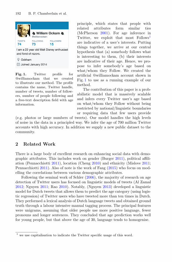
192 B. P. Chamberlain et al.
Fig. 1. Twitter profile for@williamockam that we createdto illustrate our method. The profilecontains the name, Twitter handle,number of tweets, number of follow-ers, number of people following anda free-text description field with ageinformation.
principle, which states that people withrelated attributes form similar ties(McPherson 2001). For age inference inTwitter, we exploit that most Follows1
are indicative of a user’s interests. Puttingthings together, we arrive at our centralhypothesis that (a) somebody follows whatis interesting to them, (b) their interestsare indicative of their age. Hence, we pro-pose to infer somebody’s age based onwhat/whom they Follow. We created theartificial @williamockam account shown inFig. 1 to use as a running example of ourmethod.
The contribution of this paper is a prob-abilistic model that is massively scalableand infers every Twitter user’s age basedon what/whom they Follow without beingrestricted by national/linguistic boundariesor requiring data that few users provide
(e.g. photos or large numbers of tweets). Our model handles the high levelsof noise in the data in a principled way. We infer the age of 700 million Twitteraccounts with high accuracy. In addition we supply a new public dataset to thecommunity.
2 Related Work
There is a large body of excellent research on enhancing social data with demo-graphic attributes. This includes work on gender (Burger 2011), political affili-ation (Pennacchiotti 2011), location (Cheng 2010) and ethnicity (Mislove 2011;Pennacchiotti 2011). Also of note is the work of Fang (2015) who focus on mod-elling the correlations between various demographic attributes.
Following the seminal work of Schler (2006), the majority of research on agedetection of Twitter users has focused on linguistic models of tweets (Al Zamal2012; Nguyen 2011; Rao 2010). Notably, (Nguyen 2013) developed a linguisticmodel for Dutch tweets that allows them to predict the age category (using logis-tic regression) of Twitter users who have tweeted more than ten times in Dutch.They performed a lexical analysis of Dutch language tweets and obtained groundtruth through a labour intensive manual tagging process. The principal featureswere unigrams, assuming that older people use more positive language, fewerpronouns and longer sentences. They concluded that age prediction works wellfor young people, but that above the age of 30, language tends to homogenise.
1 we use capitalisation to indicate the Twitter specific usage of this word.
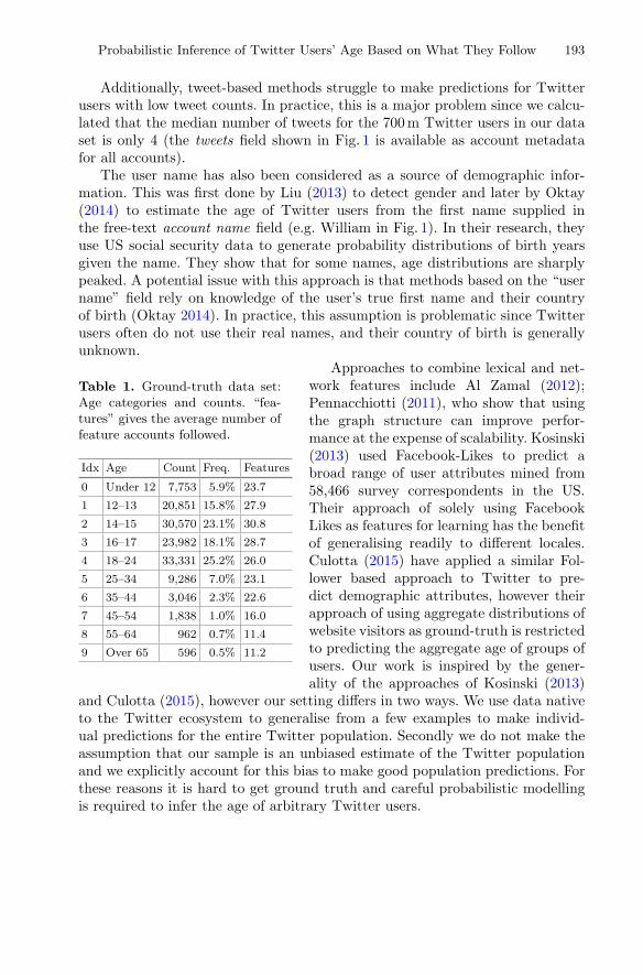
Probabilistic Inference of Twitter Users’ Age Based on What They Follow 193
Additionally, tweet-based methods struggle to make predictions for Twitterusers with low tweet counts. In practice, this is a major problem since we calcu-lated that the median number of tweets for the 700 m Twitter users in our dataset is only 4 (the tweets field shown in Fig. 1 is available as account metadatafor all accounts).
The user name has also been considered as a source of demographic infor-mation. This was first done by Liu (2013) to detect gender and later by Oktay(2014) to estimate the age of Twitter users from the first name supplied inthe free-text account name field (e.g. William in Fig. 1). In their research, theyuse US social security data to generate probability distributions of birth yearsgiven the name. They show that for some names, age distributions are sharplypeaked. A potential issue with this approach is that methods based on the “username” field rely on knowledge of the user’s true first name and their countryof birth (Oktay 2014). In practice, this assumption is problematic since Twitterusers often do not use their real names, and their country of birth is generallyunknown.
Table 1. Ground-truth data set:Age categories and counts. “fea-tures” gives the average number offeature accounts followed.
Idx Age Count Freq. Features
0 Under 12 7,753 5.9% 23.7
1 12–13 20,851 15.8% 27.9
2 14–15 30,570 23.1% 30.8
3 16–17 23,982 18.1% 28.7
4 18–24 33,331 25.2% 26.0
5 25–34 9,286 7.0% 23.1
6 35–44 3,046 2.3% 22.6
7 45–54 1,838 1.0% 16.0
8 55–64 962 0.7% 11.4
9 Over 65 596 0.5% 11.2
Approaches to combine lexical and net-work features include Al Zamal (2012);Pennacchiotti (2011), who show that usingthe graph structure can improve perfor-mance at the expense of scalability. Kosinski(2013) used Facebook-Likes to predict abroad range of user attributes mined from58,466 survey correspondents in the US.Their approach of solely using FacebookLikes as features for learning has the benefitof generalising readily to different locales.Culotta (2015) have applied a similar Fol-lower based approach to Twitter to pre-dict demographic attributes, however theirapproach of using aggregate distributions ofwebsite visitors as ground-truth is restrictedto predicting the aggregate age of groups ofusers. Our work is inspired by the gener-ality of the approaches of Kosinski (2013)
and Culotta (2015), however our setting differs in two ways. We use data nativeto the Twitter ecosystem to generalise from a few examples to make individ-ual predictions for the entire Twitter population. Secondly we do not make theassumption that our sample is an unbiased estimate of the Twitter populationand we explicitly account for this bias to make good population predictions. Forthese reasons it is hard to get ground truth and careful probabilistic modellingis required to infer the age of arbitrary Twitter users.

194 B. P. Chamberlain et al.
3 Probabilistic Age Inference in Twitter
Our age inference method uses ground-truth labels (users who specify their age),which are then generalised to 700 m accounts based on the shared interests, whichwe derive from Following patterns.
To extract ground-truth labels we crawl the Twitter graph and download userdescriptions. To do this we implemented a distributed Web crawler using Twitteraccess tokens mined through several consumer apps. To maximize data through-put while remaining within Twitter’s rate limits we built an asynchronous datamining system connected to an access token server using Python’s Twistedlibrary Wysocki (2011).
Table 2. Public datasetlabels: age categories andcounts.
Idx Age range Count
1 10–19 4486
2 20–29 4485
3 30–39 4487
4 40–49 4485
5 50–59 4484
6 60–69 4481
7 70–79 4481
Our crawl downloaded 700 m user descriptions.Fig. 1 shows the profile with associated metadata fieldsfor the fictitious @williamockam account, which weuse to illustrate our approach. We index the free-text description fields using Apache SOLR (Grainger2014) and search the index for REGular EXpression(REGEX) patterns that are indicative of age (e.g., thephrase: “I am a 22 year old” in Fig. 1) across Twit-ter’s four major languages (English, Spanish, French,Portuguese). For repeatability we include our REGEXcode in the git repository. Twitter is ten years oldand contains many out-of-date descriptions. To tacklethe stale data problem we restricted the ground-truthto active accounts, defined to be accounts that hadtweeted or Followed in the last three months (we donot have access to Twitter’s logs). This process dis-covered 133,000 active users who disclosed their age(i.e., 0.02% of the 700 m indexed accounts), which weuse as “ground-truth” labels. For each of these we download every account thatthey Followed. Figure 1 shows that @williamockam Follows 73 accounts and wedownloaded each of their user IDs. We use ten age categories with a higher res-olution in younger ages where there is more labelled data. For our ground-truthdata set, the age categories, number of accounts, relative frequency and averagenumber of features per category are shown in Table 1.
Applying REGEX matches to free-text fields inevitably leads to some falsepositives due to unanticipated character combinations when working with largedata sets. In addition, many Twitter accounts, while correctly labelled, may notrepresent the interests of human beings. This can occur when accounts are con-trolled by machines (bots), accounts are set up to look authentic to distributespam (spam accounts) or account passwords are hacked in order to sell authenticlooking Followers. To reduce the impact of spurious accounts on the model wenote that (1) incorrectly labelled accounts can have a large effect on the model as

Probabilistic Inference of Twitter Users’ Age Based on What They Follow 195
they are distant in feature space from other members of the class/label (2) incor-rectly labelled accounts that have a small effect on the model (e.g. because theyonly follow one popular feature) do not matter much by definition. To measurethe effect of each labelled account on the model we compute the Kullback-Leiblerdivergence KL(P ||P\i) between the full model and a model evaluated with onedata point missing. Here, P is the likelihood of the full, labelled data set, andP\i is the likelihood of the model using the labelled data set minus the ith datapoint. This methodology identifies any accounts that have a particularly largeimpact on our predictive distribution. We flagged any training examples thatwere more than three median absolute deviations from the median score formanual inspection. This process excluded 246 accounts from our training dataand examples are shown in Table 3. We also randomly sampled 100 data pointsfrom across the full ground-truth set and manually verified them by inspectingthe descriptions, tweets and who/what they Follow.
Table 3. Spurious data points identified by taking the Median Absolute Deviation ofthe leave-one-out KL-Divergence.
Handle Twitter description REGEX age Reason to exclude
RIAMOpera Opera at the Royal Irish...Presenting: Ormindo Jan 11
11 An Irish Opera
TiaKeough13 My name Tia I’m 13 yearsold
13 Hacked account
39yearoldvirgin I’m 39 years old... if you’re awoman, I want to meet you
39 Probably not 39
50Plushealths Retired insurance AgentAfter 40 years of services
Retired Using reciprocation software
MrKRudd Former PM of Australia...Proud granddad of Josie &McLean
Grandparent Outlier. Former AUS PM
For reproducibility we make an anonymised sample of the data and our codepublicly available2. The data is in two parts: (1) A sparse bipartite adjacencymatrix; (2) a vector of age category labels. This dataset was collected and cleanedaccording to the methodology described above and then down-sampled to giveapproximately equal numbers of labels in each of seven classes detailed in Table 2.It includes only accounts that explicitly state an age (i.e. no grandparents orretirees). The adjacency matrix is in the format of a standard (sparse) designmatrix and includes only features that are Followed by at least 10 examples. Thehigh level statistics of this network are described in Table 4.
2 https://github.com/melifluos/bayesian-age-detection.

196 B. P. Chamberlain et al.
3.1 Age Inference Based on Follows
Given a set of 133,000 labelled data points (ground-truth, i.e., Twitter users whoreveal their age) we wish to infer the age of the remaining 700 m Twitter users.For this purpose, we define a set of features that can be extracted automatically.The features are based on the Following patterns of Twitter users. Once thefeatures are defined, we propose a scalable probabilistic model for age inference.
Table 4. Public datasetadjacency matrix statis-tics. Subscript 1 describeslabelled acounts and 2describes features. Vdenotes vertices, E edgesand D degree.
Attribute Value
|V1| 31,389
|V2| 50,190
|E| 1,810,569
avg D1 57.7
max D1 2049
std D1 95.2
avg D2 36.1
max D2 4405
std D2 96.2
Our age inference exploits the hypothesis thatsomeone’s interests are indicative of their age, anduses Twitter Follows as a proxy for interests. There-fore, the features of our model are the 103,722 Twitteraccounts that are Followed by more than ten labelledaccounts, which can be found automatically. Of the73 accounts Followed by @williamockam, 8 had suf-ficient support to be included in our model. Thesewere: Lord Voldemort7, WaltDisneyWorld, Apple-bees, UniStudios, UniversalORL, HorrorNightsORL,HorrorNights and OlanRogers.
Table 5 shows the number of labelled accounts Fol-lowing each feature for @williamockam. The supportis the number of labelled Followers summed over allage categories, while Followers gives the total num-ber of Followers (labelled and unlabelled). A generaltrend across all features (not only the ones relevant to@williamockam) is that the age distribution is peakedtowards “younger” ages as not many older peoplereveal their age (we show this for the accounts withthe highest support in our data set in the appendixon our git repo). To improve the predictive perfor-mance of the model in higher age categories we adapted our REGEX to searchfor grandparents and retirees. This augmented our training data with 176,748
Table 5. Follower counts for the eight @williamockam features. The support gives theirtotal number of Followers in our labelled data set and Followers is their total numberon Twitter. Fractional counts are from assigning a distribution to grandparents.
Twitter handle Support <12 12–13 14–15 16–17 18–24 25–34 35–44 45–54 55–64 ≥65 Followers
Lord Voldemort7 273 5 35 75 55 87 13 0 1 1 1 2.0×10⁶
WaltDisneyWorld 435 61 100 89 80 65 20 4 7 4 4 2.5×10⁶
Applebees 191 18 43 38 30 37 9 8 2.33 2.33 3.33 0.57×10⁶
UniStudios 60 7 7 14 14 13 5 0 0 0 0 0.27×10⁶
UniversalORL 65 5 13 10 15 14 4 0 1.66 1.66 0.66 0.40×10⁶
HorrorNightsORL 5 0 0 0 1 3 1 0 0 0 0 0.04×10⁶
HorrorNights 18 1 3 1 4 6 0 1 0.66 0.66 0.66 0.08×10⁶
OlanRogers 16 0 2 0 7 7 0 0 0 0 0 0.11×10⁶

Probabilistic Inference of Twitter Users’ Age Based on What They Follow 197
Table 6. Posterior distributions (4) for the eight features Followed by @williamockam.Probabilities are ×10−5
Twitter handle Support <12 12–13 14–15 16–17 18–24 25–34 35–44 45–54 55–64 ≥65 Followers
Lord Voldemort7 273 111.7 190.9 258.0 252.3 248.6 145.9 31.9 38.9 77.6 177.5 2.0×10⁶
WaltDisneyWorld 435 725.0 538.2 441.2 377.6 267.3 233.2 194.2 270.7 254.5 224.4 2.5×10⁶
Applebees 191 231.8 206.3 176.6 150.3 129.8 137.4 226.7 132.4 139.6 139.2 0.57×10⁶
UniStudios 60 80.6 56.0 59.3 59.5 49.3 48.1 11.3 2.8 2.3 2.3 0.27×10⁶
UniversalORL 65 67.4 63.0 56.6 60.5 50.7 42.0 21.1 62.7 86.4 40.6 0.40×10⁶
HorrorNightsORL 5 0.3 0.7 1.5 4.0 8.3 9.4 2.0 0.3 0.1 0.1 0.04×10⁶
HorrorNights 18 14.0 13.7 11.3 15.5 16.1 9.4 29.1 29.9 36.8 29.3 0.08×10⁶
OlanRogers 16 4.3 9.1 10.6 21.9 19.8 5.0 1.6 1.3 1.3 1.3 0.11×10⁶
people labelled as retired and 63,895 labelled as grandparents. In our ten-category model, retired people are added to the 65+ category. Grandparentsare assigned a uniform distribution across the three oldest age categories, whichroughly reflects the age distribution of grandparents in the US (UScensus 2014)3,such that we ended up with approximately 374,000 labelled accounts in ourground-truth data.
Probabilistic Model for Age Inference. We adopt a Bayesian classificationparadigm as this provides a consistent framework to model the many sources ofuncertainty (noisy labels, noisy features, survey estimates) encountered in theproblem of age inference.
Our goal is to predict the age label of an arbitrary Twitter user with featurevector X given the set of feature vectors X and corresponding ground-truthage labels A. Within a Bayesian framework, we are therefore interested in theposterior predictive distribution
P (A|X,X,A) ∝ P (X|A,X,A)P (A) , (1)
where P (A) is the prior age distribution and P (X|A,X,A) the likelihood.The prior P (A) is based on a survey of American internet users conducted
by Duggan (2013). They sampled 1,802 over-18-year olds using random coldcalling and recorded their demographic information and social media use. 288 oftheir respondents were Twitter users, yielding a small data set that we use forthe prior distributions of over 18 s. For under 18 s we inferred the correspondingvalues of the prior using US census data (UScensus 2010), which leads to thecategorical prior
P (A) = Cat(π) = [1, 2, 2, 3, 14, 23, 23, 22, 6, 4] × 10−2 . (2)
3 This value was used as the US is the largest Twitter country.

198 B. P. Chamberlain et al.
The likelihood P (X|A,X,A) is obtained as follows: For scalability we makethe Naive Bayes assumption that the decision to Follow an account is indepen-dent given the age of the user. This yields the likelihood
P (X|A,X,A) =∏M
i=1P (Xi|A,A,X)Xi , (3)
where Xi ∈ {0, 1} and i indexes the features. Xi = 1 means “user χ Followsfeature account i”.4
We model the likelihood factors P (Xi|A,A,X) as Bernoulli distributions
P (Xi|A = a) = Ber(μia), (4)
i = 1, . . . ,M , where M is the number of features and there are 10 age cat-egories indexed by a = 1, . . . , 10. Since our labelled data is severely biasedtowards “younger” age categories we cannot simply learn multinomial distribu-tions P (A|Xi) for each feature based on the relative frequencies of their followers(see Table 1). To smooth out noisy observations of less popular accounts we usea hierarchical Bayesian model. Inference is simplified by using the Bernoulli’sconjugate distribution, the beta distribution
Beta(μia|bia, ca) (5)
on the Bernoulli parameters μia. We seek hyper-parameters bia, cia of the priorBeta(μia|X,A), which do not have a large effect when ample data is available,but produce sensible distributions when it is not. To achieve this we set ca to beconstant across all features Xi (hence dropping the i subscript) and proportionalto the total number of observations na in each age category (the count columnin Table 1). We then set bia ∝ nani
K , where K = 7 × 10⁸ is the total number ofTwitter users and ni is the number of Followers of feature i (the Followers columnof Table 5 for @williamockam’s features). Then, the expected prior probabilitythat user χ Follows account i is E[μia|A = a] = bia
bia+ca= ni
K+ni, i.e., it is
constant across age classes and varies in proportion to the number of Followersacross features. The effect of this procedure is to reduce the model confidencefor features where data is limited. Due to conjugacy, the posterior distributionon μia is also Beta distributed. Integrating out μia we obtain
P (Xi = 1|A=a,X,A) =
1∫
0
P (Xi=1|μi, A)P (μi|X,A, A)dμi (6)
=
1∫
0
μiaP (μia|X,A)dμia = E[μia|X,A] = nia+biana+bia+ca
, (7)
4 We only consider cases where Xi = 1 since the Twitter graph is sparse: In the fullTwitter graph there are 7 × 10⁸ nodes with 5 × 10¹⁰ edges, which implies a densityof 1.6 × 10⁻⁷, i.e., the default is to follow nobody. Hence, not following an accountdoes not contain enough information to justify the additional computational cost.

Probabilistic Inference of Twitter Users’ Age Based on What They Follow 199
Fig. 2. Receiver operator characteristicsfor three class age detection (0 = under18, 1 = 18–45, 2 = 45+). The dashed lineindicates random performance.
where nia is the number of labelledTwitter users in age category a whoFollow feature Xi, which are givenin Table 5 for the @williamockam fea-tures and na is the number of Twit-ter users in category a in the ground-truth (See Table 1). Performing thiscalculation yields the likelihoods forthe @williamockam features shown inTable 6. We are now able to computethe predictive distribution in (1) toinfer the age of an arbitrary Twitteruser. The predictive distribution for@williamockam is shown in Fig. 4 andis calculated by taking the product ofthe likelihoods from Table 6 with theprior in (2) and normalising.
The generative process in our model for the likelihood term in (1) is as follows.
1. Draw an age category A ∼ Cat(π)2. For each feature i draw μia ∼ Beta(μia|bia, ca)3. For each account draw the Follows: Xi ∼ Ber(μia)
Table 7. The most discriminative features based on the posterior distribution over agein (6). Descriptions are taken from the 1st line of their Wikipedia pages. See the gitrepo for a full table with probabilities and handles.
<12 12–13 14–15 16–17 18–24
Vlogger Child presenter Child singer Singer Metalcore band
Minecraft gamer YouTuber Child singer Metalcore band Rock band
Internet personality Child actress Child singer Deathcore singer Rapper
Vlogger Child actress Child singer
Gaming commentator Girl band Child singer Electronic band Rock band
25–34 35–44 45–64a 65+
Hip hop duo Hip hop artist Evangelist Political journalist
Boy band Rapper Evangelist Retired cyclist
Boy band History channel Evangelist Golf channel
Comedian Record label Faith group Retired rugby player
Adult actress Boxer Faith magazine BoxeraBoth categories have the same features
In Table 7, we report the five features with the highest posterior age valuesof P (A|Xi = 1) for each age category. The account descriptions are taken fromthe first line of the relevant Wikipedia page. The youngest Twitter users arecharacterised by an interest in internet celebrities and computer games players.Music genres are important in differentiating all age groups from 12–45. 25–34
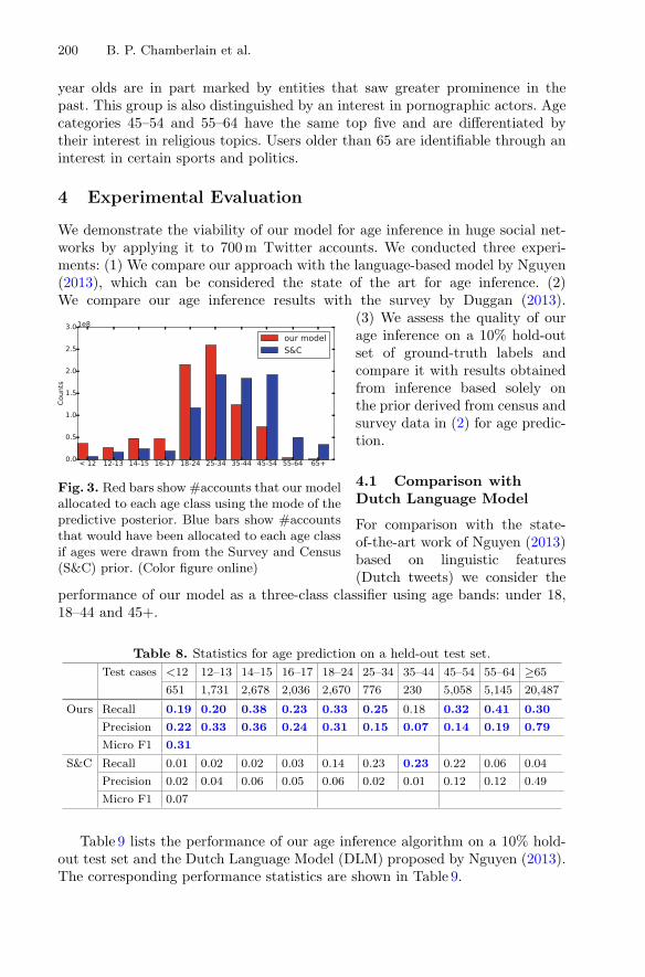
200 B. P. Chamberlain et al.
year olds are in part marked by entities that saw greater prominence in thepast. This group is also distinguished by an interest in pornographic actors. Agecategories 45–54 and 55–64 have the same top five and are differentiated bytheir interest in religious topics. Users older than 65 are identifiable through aninterest in certain sports and politics.
4 Experimental Evaluation
We demonstrate the viability of our model for age inference in huge social net-works by applying it to 700 m Twitter accounts. We conducted three experi-ments: (1) We compare our approach with the language-based model by Nguyen(2013), which can be considered the state of the art for age inference. (2)We compare our age inference results with the survey by Duggan (2013).
Fig. 3. Red bars show #accounts that our modelallocated to each age class using the mode of thepredictive posterior. Blue bars show #accountsthat would have been allocated to each age classif ages were drawn from the Survey and Census(S&C) prior. (Color figure online)
(3) We assess the quality of ourage inference on a 10% hold-outset of ground-truth labels andcompare it with results obtainedfrom inference based solely onthe prior derived from census andsurvey data in (2) for age predic-tion.
4.1 Comparison withDutch Language Model
For comparison with the state-of-the-art work of Nguyen (2013)based on linguistic features(Dutch tweets) we consider the
performance of our model as a three-class classifier using age bands: under 18,18–44 and 45+.
Table 8. Statistics for age prediction on a held-out test set.
Test cases <12 12–13 14–15 16–17 18–24 25–34 35–44 45–54 55–64 ≥65
651 1,731 2,678 2,036 2,670 776 230 5,058 5,145 20,487
Ours Recall 0.19 0.20 0.38 0.23 0.33 0.25 0.18 0.32 0.41 0.30
Precision 0.22 0.33 0.36 0.24 0.31 0.15 0.07 0.14 0.19 0.79
Micro F1 0.31
S&C Recall 0.01 0.02 0.02 0.03 0.14 0.23 0.23 0.22 0.06 0.04
Precision 0.02 0.04 0.06 0.05 0.06 0.02 0.01 0.12 0.12 0.49
Micro F1 0.07
Table 9 lists the performance of our age inference algorithm on a 10% hold-out test set and the Dutch Language Model (DLM) proposed by Nguyen (2013).The corresponding performance statistics are shown in Table 9.
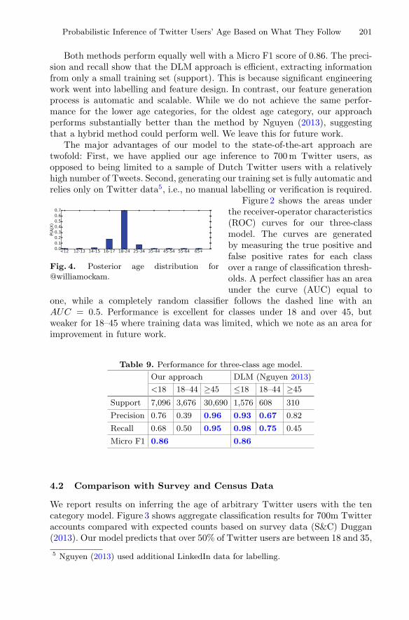
Probabilistic Inference of Twitter Users’ Age Based on What They Follow 201
Both methods perform equally well with a Micro F1 score of 0.86. The preci-sion and recall show that the DLM approach is efficient, extracting informationfrom only a small training set (support). This is because significant engineeringwork went into labelling and feature design. In contrast, our feature generationprocess is automatic and scalable. While we do not achieve the same perfor-mance for the lower age categories, for the oldest age category, our approachperforms substantially better than the method by Nguyen (2013), suggestingthat a hybrid method could perform well. We leave this for future work.
The major advantages of our model to the state-of-the-art approach aretwofold: First, we have applied our age inference to 700 m Twitter users, asopposed to being limited to a sample of Dutch Twitter users with a relativelyhigh number of Tweets. Second, generating our training set is fully automatic andrelies only on Twitter data5, i.e., no manual labelling or verification is required.
Fig. 4. Posterior age distribution for@williamockam.
Figure 2 shows the areas underthe receiver-operator characteristics(ROC) curves for our three-classmodel. The curves are generatedby measuring the true positive andfalse positive rates for each classover a range of classification thresh-olds. A perfect classifier has an areaunder the curve (AUC) equal to
one, while a completely random classifier follows the dashed line with anAUC = 0.5. Performance is excellent for classes under 18 and over 45, butweaker for 18–45 where training data was limited, which we note as an area forimprovement in future work.
Table 9. Performance for three-class age model.
Our approach DLM (Nguyen 2013)
<18 18–44 ≥45 ≤18 18–44 ≥45
Support 7,096 3,676 30,690 1,576 608 310
Precision 0.76 0.39 0.96 0.93 0.67 0.82
Recall 0.68 0.50 0.95 0.98 0.75 0.45
Micro F1 0.86 0.86
4.2 Comparison with Survey and Census Data
We report results on inferring the age of arbitrary Twitter users with the tencategory model. Figure 3 shows aggregate classification results for 700m Twitteraccounts compared with expected counts based on survey data (S&C) Duggan(2013). Our model predicts that over 50% of Twitter users are between 18 and 35,
5 Nguyen (2013) used additional LinkedIn data for labelling.
202 B. P. Chamberlain et al.
i.e., the bias of the original training set has been removed due to the Bayesiantreatment. It is likely that S&C under-represents young people as we did notfactor in the increased rates of technology uptake amongst the younger peoplewhen converting census data.
4.3 Quality Assessment
In the following, we assess the quality of our age inference model (10 categories)on a 10% hold-out test data set.
Table 8 shows the performance statistics for this experiment. The majorityof the test cases are in the younger age categories (due to the bias of youngpeople revealing their age) and in older age categories (due to the inclusion ofgrandparents and retirees). Table 8 shows that the precision depends on the sizeof the data (e.g., predicting 25–44 year categories is hard) whereas the recall isfairly stable across all age categories.6 Our model significantly outperforms anapproach based only on the survey and census data (S&C), which we use as aprior. This highlights the ability of our model to adapt to the data.
5 Conclusion
We proposed a probabilistic model for age inference in Twitter. The modelexploits generic properties of Twitter users, e.g., whom/what they follow, whichis indicative of their interests and, therefore, their age. Our model performs aswell as the current state of the art for inferring the age of Twitter users withoutbeing limited to specific linguistic or engineered features. We have successfullyapplied our model to infer the age of 700 million Twitter users demonstratingthe scalability of our approach. The method can be applied to any attributesthat can be extracted from user profiles.
Acknowledgements. This work was partly funded by an Industrial Fellowship fromthe Royal Commission for the Exhibition of 1851. The authors thank the anonymousreviewers for providing many improvements to the original manuscript.
References
Al Zamal, F., Liu, W., Ruths, D.: Homophily and latent attribute inference: inferringlatent attributes of twitter users from neighbors. In: ICWSM (2012)
Burger, J.D., Henderson, J., Kim, G., Zarrella, G.: Discriminating gender on Twitter.In: EMNLP (2011)
Cheng, Z., Caverlee, J., Lee, K.: You are where you tweet: a content-based approachto geo-locating Twitter users. In: CIKM (2010)
Culotta, A., Nirmal, R.K., Cutler, J.: Predicting the demographics of Twitter usersfrom website traffic data. In: AAAI (2015)
6 Without the inclusion of grandparents and retirees in the training set, the predictiveperformance would rapidly drop off for ages greater than 35.
Probabilistic Inference of Twitter Users’ Age Based on What They Follow 203
Duggan, M., Brenner, J.: The demographics of social media Users–2012. http://tinyurl.com/jk3v9tu. Retrieved 12 Sep 2015
Fang, Q., Sang, J., Xu, C., Hossain, M.S.: Relational user attribute inference in socialmedia. IEEE Trans. Multimedia 17(7), 1031–1044 (2015)
Grainger, T., Potter, T.: Solr in Action. Manning Publications Co., Cherry Hill (2014)Gupta, P., Goel, A., Lin, J., Sharma, A., Wang, D., Zadeh, R.: WTF: the who to follow
service at Twitter. In: WWW (2013)Kosinski, M., Stillwell, D., Graepel, T.: Private traits and attributes are predictable
from digital records of human behavior. PNAS 110(15), 5802–5805 (2013)Liu, W., Ruths, D.: Whats in a name? using first names as features for gender inference
in Twitter. In: AAAI Spring Symposium on Analyzing Microtext (2013)McPherson, M., Smith-Lovin, L., Cook, J.M.: Birds of a feather: homophily in social
networks. Ann. Rev. Sociol. 27(1), 415–444 (2001)Mislove, A., Lehmann, S., Ahn, Y.Y.: Understanding the demographics of Twitter
users. In: ICWSM (2011)Nguyen, D., Gravel, R., Trieschnigg, D., Meder, T.: How old do you think i am? a
study of language and age in Twitter. In: ICWSM (2013)Nguyen, D., Noah, A., Smith, A., Rose, C.P.: Author age prediction from text using
linear regression. In: LaTeCH (2011)Oktay, H., Firat, A., Ertem, Z.: Demographic breakdown of Twitter users: an analysis
based on names. In: BIGDATA (2014)Pennacchiotti, M., Popescu, A.M.: A machine learning approach to Twitter user clas-
sification. In: ICWSM (2011)Rao, D., Yarowsky, D., Shreevats, A., Gupta, M.: Classifying latent user attributes in
Twitter. In: SMUC (2010)Schler, J., Koppel, M., Argamon, S., Pennebaker, J.W.: Effects of age and gender on
blogging. In: AAAI-CAAW (2006)Wysocki, R., Zabierowski, W.: Twisted framework on game server example. In: CADSM
(2011)U.S. Census Bureau, 2010 Census. Profile of General Population and Housing Charac-
teristics: 2010. https://goo.gl/VAGMNl. Retrieved 12 Sep 2015U.S. Census Bureau, American Community Survey, 2014 Grandparent Statistics.
https://goo.gl/CqGXWI. Retrieved 15 Nov 2015

Quantifying Heterogeneous Causal TreatmentEffects in World Bank Development
Finance Projects
Jianing Zhao1(B), Daniel M. Runfola2, and Peter Kemper1
1 College of William and Mary, Williamsburg, VA 23187-8795, USA{jzhao,kemper}@cs.wm.edu
2 AidData, 427 Scotland Street, Williamsburg, VA 23185, [email protected]
Abstract. The World Bank provides billions of dollars in developmentfinance to countries across the world every year. As many projects arerelated to the environment, we want to understand the World Bankprojects impact to forest cover. However, the global extent of theseprojects results in substantial heterogeneity in impacts due to geo-graphic, cultural, and other factors. Recent research by Athey andImbens has illustrated the potential for hybrid machine learning andcausal inferential techniques which may be able to capture such hetero-geneity. We apply their approach using a geolocated dataset of WorldBank projects, and augment this data with satellite-retrieved character-istics of their geographic context (including temperature, precipitation,slope, distance to urban areas, and many others). We use this informationin conjunction with causal tree (CT) and causal forest (CF) approachesto contrast ‘control’ and ‘treatment’ geographic locations to estimate theimpact of World Bank projects on vegetative cover.
1 Introduction
We frequently seek to test the effectiveness of targeted interventions - for exam-ple, a new website design or medical treatment. Here, we present a case study ofusing recent theoretical advances - specifically the use of tree-based analysis [3] -to estimate heterogeneous causal effects of global World Bank projects on forestcover over the last 30 years.
The World Bank is one of the largest contributors to development financein the world, seeking to promote human well-being through a wide variety ofprograms and related institutions [1]. However, this goal is frequently at oddswith environmental sustainability - building a road can necessitate the removal oftrees; building a factory that supplies jobs can lead to the pollution of proximateforests. Multiple environmental safeguards have been put in place to offset thesechallenges, but relatively little is known about their efficacy across large scales.
We adopt the commonly applied approach of selecting “control” cases (i.e.,areas where World Bank projects have very little funding) to contrast toc© Springer International Publishing AG 2017Y. Altun et al. (Eds.): ECML PKDD 2017, Part III, LNAI 10536, pp. 204–215, 2017.https://doi.org/10.1007/978-3-319-71273-4_17

Quantifying Causal Effects in World Bank Development Finance Projects 205
“treated” cases (i.e., areas where World Bank projects have a large amountof funding). This is analogous to similar approaches in the medical literature,where humans are put into control and treatment groups, and individuals thatare similar along all measurable attributes are contrasted to one another after amedicine is administered. This is necessary due to the generalized challenge ofall observational studies: it is impossible observe the exact same unit of observa-tion with and without a World Bank project simultaneously - in the same wayit would be impossible to examine a patient that was and was not given med-ication at the same time. Further complicating the challenge presented in thispaper is the scope of the World Bank - with tens of thousands of project loca-tions worldwide, there is considerable variation in the aims of different projects,the project’s size, location, socio-economic, environmental, and historical set-tings. This variation makes traditional, aggregate estimates of impact unhelpful,as such aggregates mask variation in where World Bank projects may be help-ing - or harming - the environment. Following this, we investigate the researchquestion What is the impact of world bank projects on forest cover?
To examine this question, we first integrate information on the geographiclocation of World Bank projects with additional, satellite derived informationon the geographic, environmental, and economic characteristics of each project.We apply four different models to this dataset, and contrast our findings to illus-trate the various tradeoffs in these approaches. Specifically, we test TransformedOutcome Trees (TOTs), Causal Trees (CTs), Random Forest TOTs (RFTOTs),and Causal Forests (CFs). We follow the work of Athey and Imbens [3], whodemonstrated how regression trees and random forests can be adjusted to esti-mate heterogenous causal effects. This work is based on the Rubin Causal Model(or potential outcome framework), where causal effects are estimated throughcomparisons between observed outcomes and the “counterfactual” outcomes onewould have observed under the absence of an aid project [9]. While traditionaltree-based approaches rely on training with data with known outcomes, Atheyand Imbens illustrated that one can estimate the conditional average treatmenteffect on a subset with regressions trees after an appropriate data transformationprocess.
Many approaches to estimating heterogeneous effects have emerged over thelast decade. LASSO [14] and support vector machines (SVM) [15] may serveas two popular examples. For this paper, we focus on very recent tree-basedtechniques that are very promising for causal inference. In [12], Su et al. proposeda statistical test as the criterion for node splitting. In [3], Athey and Imbensderived TOTs and CTs, an idea that is followed up on by Wagner and Athey[16] with CF (causal forest, random forests of CTs), and similarly Denil et al.in [6] who use different data for the structure of the tree and the estimatedvalue within each node. Random forests naturally gave rise to the question ofconfidence intervals for the estimates they deliver. Following this, Meinshausenintroduced quantile regression forests in [10] to estimate a distribution of results,and Wagner et al. [17] provided guidance for confidence intervals with randomforests. Several authors, including Biau [4], recognize a gap between theoreticalunderpinnings and the practical applications of random forests.

206 J. Zhao et al.
The contribution of this paper is twofold: we evaluate and compare a numberof proposed methods on simulated data where the ground truth is known andapply the most promising for the analysis of a real world data set. Practicalexperience results on tree-based causal inference methods are rare. To the bestof our knowledge, this is the first investigation on the analysis of a spatial dataset of world wide range with a large scale set of projects and dimensions. Whenit comes to applications for causal inference techniques, A/B testing for websites(such as eBay) is a more common [13]. A/B testing is conducted by divertingsome percentage of traffic for a website A to a modified variant B of said websitefor evaluation purposes. This leads to a large amount of data with clearly definedtreated and untreated groups where cases vary mainly by user activity. Whilethe difference between A and B is precisely defined and typically small, the hugenumber of cases helps to recognize treatment effects. This is very different tothe World Bank data which is both much more limited in size, and also spreadall over the world (resulting in large diversity across projects). The rest of thepaper is structured as follows. In Sect. 2, we present the basic methodology for thecalculation of CT and CF. Section 3 introduces the data set, its characteristics,preprocessing steps and the calculation of propensity scores necessary for theestimation of each type of tree. In Sect. 4, we present the outcome of the analysis.We conclude in Sect. 5.
2 Methodology
Causal inference is to a vast part a missing data problem as we can not observea unit at the same time receiving and not receiving treatment to compare theoutcomes. We introduce some notation and recall common concepts to be ableto address this problem in a more formal way.
Causal Effects. Suppose we have a data set with n independently and iden-tically distributed (iid) units Ui = (Xi, Yi) with i = 1, · · · , n. Each unit hasan observed feature vector Xi ∈ R
d, a response (i.e., the outcome of interest)Yi ∈ R and binary treatment indicator Wi ∈ {0, 1}. For a unit-level causaleffect, the Rubin causal model considers the treatment effect on unit i beingτ(Xi) = Yi(1) − Yi(0), the difference between treated Yi(1) and untreated Yi(0)outcome. One can be interested in an overall average treatment effect acrossall units U or investigate treatment effects of subsets that are characterized bytheir features X. The latter describes heterogeneous causal effects and is oftenof particular interest. In our case, it is interesting to identify characteristics ofsubsets of projects where the environment is affected strongly (positive or neg-ative) by a World Bank project. The heterogenous causal effect is defined asτ(x) = E
[Yi(1) − Yi(0) | Xi = x
]following [8].
Causal Tree. A regression tree defines a partition of a set of units Ui = (Xi, Yi)as each leaf node holds a subset of units satisfying conditions on X expressedalong the path from root node to leaf. This helps for the condition in τ(x) =E
[Yi(1) − Yi(0) | Xi = x
]. In observational studies, a unit is either treated or not,

Quantifying Causal Effects in World Bank Development Finance Projects 207
so we know either Yi(1) or Yi(0), but not both. However, one can still estimateτ(x) if one assumes unconfoundedness: Wi ⊥⊥ (Yi(1), Yi(0)) | Xi. Athey andImbens [3] showed that one can estimate the causal effect as:
τ(Xi) =∑
i∈T
Yi · Wi/e(Xi)∑j∈T Wj/e(Xj)
−∑
i∈C
Yi · (1 − Wi)/(1 − e(Xi))∑j∈C(1 − Wj)/(1 − e(Xj))
(1)
where e(Xi) is the propensity score of project i which is calculated by logisticregression, T represents treatment units, and C control units. Hence one canadapt the calculation of a regression tree to support calculation of τ(Xi) by (1)by adjusting the splitting rule in the tree generation process.
In a classic regression tree, mean square error (MSE) is often used as thecriterion for node splitting, and the average value within the node is used as theestimator. Following Athey and Imbens [3], we use (1) as the estimator and thefollowing equation as the new MSE for any given node J in the causal tree.
MSE =∑
i∈J
(Yi(1) − Yi(0) − τ(Xi))2 =∑
i∈J
τ(Xi)2 −∑
i∈J
τ(Xi)2 (2)
The right equation follows if one assumes that∑
i∈J τ(Xi) =∑
i∈J τ(Xi). Thekey observation is that
∑i∈J τ(Xi)2 is constant and does not impact ΔMSE.
For a split, data in node P is split into a left L and right R node, ΔMSE =MSEP − MSEL − MSER =
∑i∈P τ(Xi)2 − ∑
i∈L τ(Xi)2 − ∑i∈R τ(Xi)2. The
ground truth τ(Xi) cancels out in ΔMSE and we can grow the tree withoutknowledge of τ(Xi). However, there is one more constraint we need to add to thesplitting rule aside from MSE. To use (1) for the calculation of τ(Xi), neither setT nor C can be empty. Due to characteristics of the data in our applied study, wefound that cases where only C or T units existed in children naturally emerged,so we added a corresponding additional stopping criterion to the splitting ruleto prevent splits that would lead to situations where T or C had less than afixed minimum cardinality.
Causal Forest. While a single causal tree allows us to estimate the causaleffect, it leads to the problem of overfitting and subsequent challenges for pruningthe tree. A common solution is to use an ensemble method such as bootstrapaggregating or bagging, namely a variant of Breiman’s random forest [5]. Ifone applies the random forest approach to causal trees, the result is called acausal forest. Computation of a causal forest scales well as it can naturally berun in parallel. The same adjustments for generating a single CT apply to thegeneration of a random forest of CTs. We implemented a causal forest algorithmwith the help of the scikit learn package. We can estimate the causal effectτCF (Xi) from a causal forest (a set CF of causal trees) for a unit i as the averageacross the estimates obtained from its trees: τCF (Xi) = 1
|CF |∑
t∈CF τt(Xi).
3 Data
Data Pre-processing. This analysis relies on three key types of data: satellite datato measure vegetation, data on the geospatial locations of World Bank projects,

208 J. Zhao et al.
and covariate datasets1. Our primary variable of interest is the fluctuation ofvegetation proximate to World Bank projects, which is derived from long-termsatellite data [11]. There are many different approaches to using satellite data toapproximate vegetation on a global scale, and satellites have been taking imagerythat can be used for this purpose for over three decades. Of these approaches,the most frequently used is the Normalized Difference Vegetation Index (NDVI),which has the advantage of the longest continuous time record. NDVI measuresthe relative absorption and reflectance of red and near-infrared light from plantsto quantify vegetation on a scale of −1 to 1, with vegetated areas falling between0.2 and 1 [7]. While the NDVI does have a number of challenges - including apropensity to saturate over densely vegetated regions, the potential for atmo-spheric noise (including clouds) to incorrectly offset values, and reflectances frombright soils providing misleading estimates - the popularity of this measurementhas led to a number of improvements over time to offset many of these errors.This is especially true of measurements from longer-term satellite records, suchas those used in this analysis, produced from the MODIS and AVHRR satelliteplatforms [11].
The second primary dataset used in this analysis measures where - geographi-cally - World Bank projects were located. This dataset was produced by [2], rely-ing on a double-blind coding system where two experts independently assign lat-itude and longitude coordinates, precision codes, and standardized place namesto each geographic feature. Disagreements are then arbitrated by a third party.
In addition to the project name, the World Bank provided information on theamount of funding for each project and the year it was implemented, alongside anumber of other ancillary variables. The database also provides information onthe number of locations associated with each project - i.e., a single project maybuild multiple schools. These range from n = 1 to n = 649 project locations fora single project.
Data Characteristics. The temporal coverage of the covariates is variable acrosssources. For NDVI, precipitation, and temperature we have highly granular,yearly information on characteristics at each World Bank project location. Fromthis information, we generate additional information regarding the trend (pos-itive or negative) before and after project implementation, as well as simpleaverages in the pre- and post periods. Many variables only have a single mea-surement - population density, accessibility to urban areas, slope, and elevationare all measured circa 2000, while distances to roads and rivers are measuredcirca 2010. Figure 1(a) shows average annual NDVI values of all project locationsfor each year since 1982. The mean values are non-negative for all projects overall years, and typical values are around 0.2 which is a lower bound for areas withvegetation. Figure 1(b) shows the distributions of slope values for a time seriesof NDVI values that starts in 1982 and ends with the year before each projectstarts. Approximately 75% of all projects have an upward trend in NDVI valuesacross this time period. Figure 1(c) shows that treated and control projects have
1 For detailed information, check https://github.com/zjnsteven/appendix.

Quantifying Causal Effects in World Bank Development Finance Projects 209
0.0
0.2
0.4
0.619
82
1983
1984
1985
1986
1987
1988
1989
1990
1991
1992
1993
1994
1995
1996
1997
1998
1999
2000
2001
2002
2003
2004
2005
2006
2007
2008
2009
2010
2011
2012
2013
2014
Year
ND
VI A
vera
ge V
alue
(a)
−0.008
−0.004
0.000
0.004
2000
2001
2002
2003
2004
2005
2006
2007
2008
2009
2010
2011
Year
ND
VI T
rend
(b) (c)
Fig. 1. Properties of NDVI values at World Bank project locations
very similar empirical distributions for changes in NDVI values when the pre-and post- averages are contrasted.
Data Interpretation for the Context of Measuring Heterogenous TreatmentEffects. One key attribute of causal attribution is a dataset which distinguishesbetween treated and untreated cases. In the case of a clinical trial, humanbeings who receive treatment might be contrasted to a control group of otherhumans of similar characteristics who do not receive a treatment. Because WorldBank projects either exist or not, here we attempt to replicate the treated anduntreated conditions by contrasting World Bank projects that were funded atvery low levels (“control”) to those that were funded at high levels (“treated”).This is reflective of a hypothesis that the observed treatment effect should pos-itively correlate with the amount of funding, i.e., huge amounts of funding areexpected to have a bigger effect than small amounts of funding. Following this,we assign Wi = 1 if a project’s funding is in the upper third of all funded projects.While an imperfect representation of an area at which no World Bank projectexists, by leveraging locations where a World Bank project exists but at a verylow intensity we mitigate potential confounding sources of bias associated withlocations the World Bank chooses to site projects at. Further, we bias our resultsin the more conservative negative direction - i.e., we will tend to under-estimatethe impact of World Bank projects relative to null cases. Future research willconsider the difference between this and a true null case in which locations withno aid at them are contrasted.
As a single project typically takes place at several project locations, we con-sider each project location as an individual unit - i.e., a school may be effec-tive in one location, but not another, even if they were implemented by thesame funding mechanism. Further, to capture potential geographic heterogene-ity this might introduce, for each unit’s feature vector (i.e., selected covariates),we include the longitude and latitude of the project location. The total length ofthe feature vector is d = 40. All covariates are numerical and their values are notnormalized. For our outcome measure (i.e., the variable we seek to estimate theimpact on), we contrast the pre-treatment and post-treatment average NDVIvalues at a project’s location. Let ndvii(92, 03) denote the average of NDVI

210 J. Zhao et al.
values observed for project location i over the years from 1992 to 2003 (the yearbefore the project is implemented, which varies across projects; 2003 is used herefor illustration). Let ndvii(05, 12) describe the corresponding value for the eightyears after the project starts. The response Yi = ndvii(05, 12) − ndvii(92, 03) isthus the difference of the two averages. Figure 1(c) shows histograms of Yi val-ues for treated and control projects. In order to calculate Y ∗ for Y , we calculatethe propensity score e(x), which describes the expected likelihood of treatmentWi for a given unit of observation. As described above, while there are manymethods for estimating e(x), here we use logistic regression to provide a bettercomparison with the econometric approaches commonly employed in the inter-national aid community.
4 Experiments and Results
We follow a two stage procedure to examine the effectiveness of both the CTand CF algorithms, specifically considering our unique context of the effective-ness of World Bank projects. First, we test and evaluate which approach ismost suited to our application using simulated synthetic data where we knowthe ground truth and where we can vary the size of sample data. Second, weapply these algorithms to examine the efficacy of World Bank projects based onsatellite imagery. We implemented the CT and CF algorithms as well as Atheyand Imbens transformed outcome tree (TOT) approach [3] and a random forestvariant of TOT (RFTOT) using scikit-learn. The latter serve as a baseline forthe performance of CT and CF algorithms.
Experimental Results for Simulated Data. First, we iteratively simulate syntheticdatasets with known parameters to evaluate how the estimation of propensityscore, dataset size, and degree of similarity between the control and treatmentgroups impact the accuracy of the result. To do this, we follow a bi-partite datageneration process, in which two equations are used (one for treated cases andanother for control cases).
We use each of the following two equations to produce one half of all datapoints. Y 1
i gives the result for treated cases; Y 0i is for the control group. Here,
from x1 to x8, xj ∼ N (0, 1) as well as ε ∼ N (0, 1).
Yi(1) = W 1i +
k∑
j=1
xj∗W 1i +
8∑
j=1
xj+ε, Yi(0) = W 0i +
k∑
j=1
xj∗W 0i +
8∑
j=1
xj+ε (3)
As used in Table 1, k is defined as the number of covariates which contributeto heterogeneity in the causal effect. The true value of the causal effect is thenτ(Xi) = Yi(1) − Yi(0) = 1 +
∑ki=1 xi, with W 1 = 1 and W 0 = 0.
The first scenario we examine considers synthetic datasets with a random-ized treatment assignment (each unit has the same probability to be treated,e(x) = 0.5). Figure 2 shows corresponding results for n = 2000, and includesboth single tree and random forest implementations of Transformed Outcome
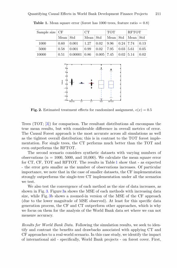
Quantifying Causal Effects in World Bank Development Finance Projects 211
Table 1. Mean square error (forest has 1000 trees, feature ratio = 0.8)
Sample size CF CT TOT RFTOT
Mean Std Mean Std Mean Std Mean Std
1000 0.60 0.001 1.27 0.02 9.96 0.24 7.74 0.13
5000 0.58 0.001 0.99 0.02 7.95 0.03 5.61 0.05
10000 0.51 0.00001 0.86 0.005 7.45 0.02 5.14 0.02
Fig. 2. Estimated treatment effects for randomized assignment, e(x) = 0.5
Trees (TOT; [3]) for comparison. The resultant distributions all encompass thetrue mean results, but with considerable difference in overall metrics of error.The Causal Forest approach is the most accurate across all simulations as wellas the tightest overall distribution; this is in contrast to the TOT forest imple-mentation. For single trees, the CT performs much better than the TOT andeven outperforms the RFTOT.
The second scenario considers synthetic datasets with varying numbers ofobservations (n = 1000, 5000, and 10,000). We calculate the mean square errorfor CT, CF, TOT and RFTOT. The results in Table 1 show that - as expected- the error gets smaller as the number of observations increases. Of particularimportance, we note that in the case of smaller datasets, the CF implementationstrongly outperforms the single-tree CT implementation under all the scenarioswe test.
We also test the convergence of each method as the size of data increases, asshown in Fig. 3. Figure 3a shows the MSE of each methods with increasing datasize, while Fig. 3b shows a zoomed-in version of the MSE of the CF approach(due to the lower magnitude of MSE observed). At least for this specific datageneration process, the CF and CT outperform other approaches, which is whywe focus on them for the analysis of the World Bank data set where we can notmeasure accuracy.
Results for World Bank Data. Following the simulation results, we seek to iden-tify and contrast the benefits and drawbacks associated with applying CT andCF approaches to a real-world scenario. In this case study, we identify the impactof international aid - specifically, World Bank projects - on forest cover. First,
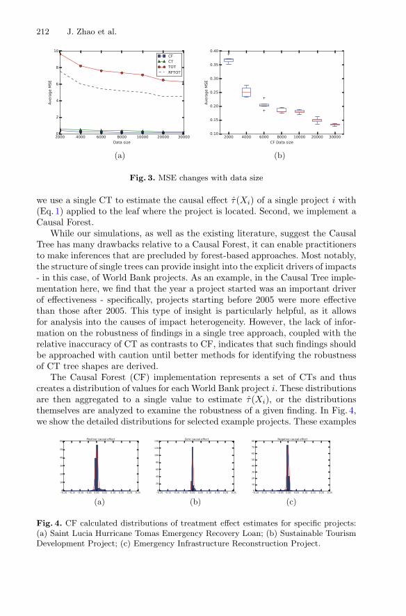
212 J. Zhao et al.
(a) (b)
Fig. 3. MSE changes with data size
we use a single CT to estimate the causal effect τ(Xi) of a single project i with(Eq. 1) applied to the leaf where the project is located. Second, we implement aCausal Forest.
While our simulations, as well as the existing literature, suggest the CausalTree has many drawbacks relative to a Causal Forest, it can enable practitionersto make inferences that are precluded by forest-based approaches. Most notably,the structure of single trees can provide insight into the explicit drivers of impacts- in this case, of World Bank projects. As an example, in the Causal Tree imple-mentation here, we find that the year a project started was an important driverof effectiveness - specifically, projects starting before 2005 were more effectivethan those after 2005. This type of insight is particularly helpful, as it allowsfor analysis into the causes of impact heterogeneity. However, the lack of infor-mation on the robustness of findings in a single tree approach, coupled with therelative inaccuracy of CT as contrasts to CF, indicates that such findings shouldbe approached with caution until better methods for identifying the robustnessof CT tree shapes are derived.
The Causal Forest (CF) implementation represents a set of CTs and thuscreates a distribution of values for each World Bank project i. These distributionsare then aggregated to a single value to estimate τ(Xi), or the distributionsthemselves are analyzed to examine the robustness of a given finding. In Fig. 4,we show the detailed distributions for selected example projects. These examples
(a) (b) (c)
Fig. 4. CF calculated distributions of treatment effect estimates for specific projects:(a) Saint Lucia Hurricane Tomas Emergency Recovery Loan; (b) Sustainable TourismDevelopment Project; (c) Emergency Infrastructure Reconstruction Project.
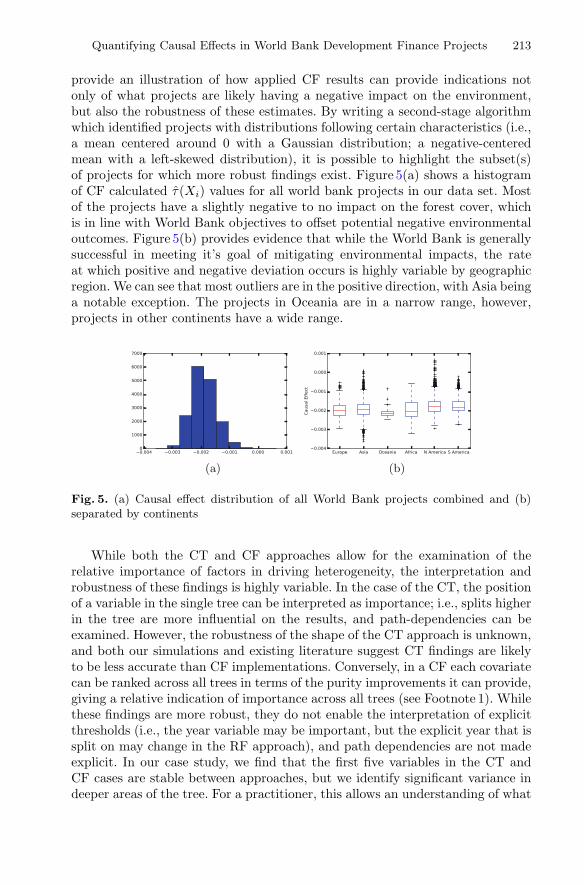
Quantifying Causal Effects in World Bank Development Finance Projects 213
provide an illustration of how applied CF results can provide indications notonly of what projects are likely having a negative impact on the environment,but also the robustness of these estimates. By writing a second-stage algorithmwhich identified projects with distributions following certain characteristics (i.e.,a mean centered around 0 with a Gaussian distribution; a negative-centeredmean with a left-skewed distribution), it is possible to highlight the subset(s)of projects for which more robust findings exist. Figure 5(a) shows a histogramof CF calculated τ(Xi) values for all world bank projects in our data set. Mostof the projects have a slightly negative to no impact on the forest cover, whichis in line with World Bank objectives to offset potential negative environmentaloutcomes. Figure 5(b) provides evidence that while the World Bank is generallysuccessful in meeting it’s goal of mitigating environmental impacts, the rateat which positive and negative deviation occurs is highly variable by geographicregion. We can see that most outliers are in the positive direction, with Asia beinga notable exception. The projects in Oceania are in a narrow range, however,projects in other continents have a wide range.
(a) (b)
Fig. 5. (a) Causal effect distribution of all World Bank projects combined and (b)separated by continents
While both the CT and CF approaches allow for the examination of therelative importance of factors in driving heterogeneity, the interpretation androbustness of these findings is highly variable. In the case of the CT, the positionof a variable in the single tree can be interpreted as importance; i.e., splits higherin the tree are more influential on the results, and path-dependencies can beexamined. However, the robustness of the shape of the CT approach is unknown,and both our simulations and existing literature suggest CT findings are likelyto be less accurate than CF implementations. Conversely, in a CF each covariatecan be ranked across all trees in terms of the purity improvements it can provide,giving a relative indication of importance across all trees (see Footnote 1). Whilethese findings are more robust, they do not enable the interpretation of explicitthresholds (i.e., the year variable may be important, but the explicit year that issplit on may change in the RF approach), and path dependencies are not madeexplicit. In our case study, we find that the first five variables in the CT andCF cases are stable between approaches, but we identify significant variance indeeper areas of the tree. For a practitioner, this allows an understanding of what

214 J. Zhao et al.
the major drivers of aid effectiveness are; for example here, the purity metrichighlights the dollars committed and environmental conditions as major driversof forest cover loss, and also highlights a disparity between projects located atdifferent latitudes; all factors which can enable a deeper understanding of whatis causing success and failure in World Bank environmental initiatives. This isconsistent with past findings which illustrate a stable set of covariates in thetop-level of trees across a CF [13]. Further, we note that the 15 most highlyranked covariates in the CF approach are generally uncorrelated, providing anindication that the information they provide is not redundant (see Footnote 1).However, we leave the interpretation of the shape of the random forest, and theinsights that can be gained from it, to future research.
5 Discussion and Conclusions
This paper sought to examine the research question What is the impact of worldbank projects on forest cover? To examine this, we contrasted four differentapproaches all based on variations of regression trees and random forests of trees:Transformed Outcome Trees (TOTs), Causal Trees (CTs), Random Forest TOTs(RFTOTs), and Causal Forests (CF). We found that the method selected canhave significant influence on the causal effect (or lack thereof) estimated, andprovide evidence suggesting CF is more accurate than alternatives in our studycontext. By applying the CF approach to the case of World Bank projects, wewere able to compute estimates for causal effects of individual projects; further,the prominent appearance of some covariates in trees provided us with guidanceon which covariates were most important in mediating the impacts of WorldBank projects. While - for most projects - the effect on forest cover is close tozero, we identified some notable exceptions, positive as well as negative ones. Wealso identified two key questions that have not yet been answered in the academicliterature. The first of these is how to select proper limitations on the makeupof terminal nodes - i.e., if splits that result in nodes without both control andtreatment cases should be prevented, omitted, or otherwise constrained. Evenafter propensity score adjustments, terminal nodes with no adequate comparisoncases become difficult (if not impossible) to interpret. Second, there is little liter-ature in the machine learning space regarding how to cope with spatial spilloverbetween treated and control cases. The Stable Unit Treatment Value Assump-tion (SUTVA) is common practice, but in practice the effects of a project can notbe expected to be purely local in nature when observations are geographicallysituated.
References
1. World Bank Group. http://www.worldbank.org/en/about/what-we-do2. AidData (2016). http://aiddata.org/subnational-geospatial-research-datasets3. Athey, S., Imbens, G.: Recursive partitioning for heterogeneous causal effects
(2015)

Quantifying Causal Effects in World Bank Development Finance Projects 215
4. Biau, G.: Analysis of a random forests model. JMLR 13(1), 1063–1095 (2012)5. Breiman, L.: Random forests. Mach. Learn. 45(1), 5–32 (2001)6. Denil, M., Matheson, D., de Freitas, N.: Narrowing the gap: random forests in
theory and in practice. In: ICML (2014)7. Dunbar, B.: NDVI: satellites could help keep hungry populations fed as climate
changes (2015). http://www.nasa.gov/topics/earth/features/obscure data.html8. Hirano, K., Imbens, G., Ridder, G.: Efficient estimation of average treatment effects
using the estimated propensity score. Econometrica 71(4), 1161–1189 (2003)9. Imbens, G.W., Rubin, D.B.: Causal Inference for Statistics, Social, and Biomedical
Sciences: An Introduction. Cambridge University Press, Cambridge (2015)10. Meinshausen, N.: Quantile regression forests. JMLR 7, 983–999 (2006)11. NASA: The land long term data record (2015). http://ltdr.nascom.nasa.gov/cgi-
bin/ltdr/ltdrPage.cgi12. Su, X., Tsai, C.L., Wang, H., Nickerson, D.M., Li, B.: Subgroup analysis via recur-
sive partitioning. J. Mach. Learn. Res. 10, 141–158 (2009)13. Taddy, M., Gardner, M., Chen, L., Draper, D.: A nonparametric Bayesian analysis
of heterogeneous treatment effects in digital experimentation (2014)14. Tibshirani, R.: Regression shrinkage and selection via the LASSO. J. R. Stat. Soc.
Ser. B 58, 267–288 (1994)15. Vapnik, V.N.: Statistical Learning Theory. Wiley-Interscience, New York (1998)16. Wager, S., Athey, S.: Estimation and inference of heterogeneous treatment effects
using random forests (2015)17. Wager, S., Hastie, T., Efron, B.: Confidence intervals for random forests: the jack-
knife and the infinitesimal jackknife. JMLR 15(1), 1625–1651 (2014)
RSSI-Based Supervised Learningfor Uncooperative Direction-Finding
Tathagata Mukherjee2(B), Michael Duckett1, Piyush Kumar1,Jared Devin Paquet4, Daniel Rodriguez1, Mallory Haulcomb1, Kevin George2,
and Eduardo Pasiliao3
1 CompGeom Inc., 3748 Biltmore Ave., Tallahassee, FL 32311, USA{michael,piyush,mallory}@compgeom.com
2 Intelligent Robotics Inc., 3697 Longfellow Road, Tallahassee, FL 32311, USA{tathagata,kevin}@intelligentrobotics.org
3 Munitions Directorate, AFRL, 101 West Eglin Blvd, Eglin AFB, FL 32542, [email protected]
4 REEF, 1350 N. Poquito Rd, Shalimar, FL 32579, [email protected]
Abstract. This paper studies supervised learning algorithms for theproblem of uncooperative direction finding of a radio emitter using thereceived signal strength indicator (RSSI) from a rotating and uncharac-terized antenna. Radio Direction Finding (RDF) is the task of findingthe direction of a radio frequency emitter from which the received sig-nal was transmitted, using a single receiver. We study the accuracy ofradio direction finding for the 2.4 GHz WiFi band, and restrict ourselvesto applying supervised learning algorithms for RSSI information anal-ysis. We designed and built a hardware prototype for data acquisitionusing off-the-shelf hardware. During the course of our experiments, wecollected more than three million RSSI values. We show that we can reli-ably predict the bearing of the transmitter with an error bounded by 11◦,in both indoor and outdoor environments. We do not explicitly modelthe multi-path, that inevitably arises in such situations and hence one ofthe major challenges that we faced in this work is that of automaticallycompensating for the multi-path and hence the associated noise in theacquired data.
Keywords: Data mining · Radio direction findingSoftware defined radio · Regression · GNURadio · Feature engineering
1 Introduction
One of the primary problems in sensor networks is that of node localization[4,9,21]. For most systems, GPS is the primary means for localizing the network.But for systems where GPS is denied, another approach must be used. A wayto achieve this is through the use of special nodes that can localize themselveswithout GPS, called anchors. Anchors can act as reference points through whichc© Springer International Publishing AG 2017Y. Altun et al. (Eds.): ECML PKDD 2017, Part III, LNAI 10536, pp. 216–227, 2017.https://doi.org/10.1007/978-3-319-71273-4_18

Uncooperative Direction-Finding 217
other nodes may be localized. One step in localizing a node is to find the directionof an anchor with respect to the node. This problem is known as Radio DirectionFinding (RDF or DF). Besides sensor networks, RDF has applications in diverseareas such as emergency services, radio navigation, localization of illegal, secretor hostile transmitters, avalanche rescue, wildlife tracking, indoor position esti-mation, tracking tagged animals, reconnaissance and sports [1,13,15,16,23,25]and has been studied extensively both for military [8] and civilian [6] use.
Direction finding has also been studied extensively in academia. One of themost commonly used algorithms for radio direction finding using the signalreceived at an antenna array is called MUSIC [22]. MUSIC and related algo-rithms are based on the assumption that the signal of interest is Gaussian andhence they use second order statistics of the received signal for determining thedirection of the emitters. Porat et al. [18] study this problem and propose theMMUSIC algorithm for radio direction finding. Their algorithm is based on theEigen decomposition of a matrix of the fourth order cumulants. Another com-monly used algorithm for determining the direction of several emitters is calledthe ESPRIT algorithm [19]. The algorithm is based on the idea of having doubletsof sensors.
Recently, researchers have used both unsupervised and supervised learningalgorithms for direction finding. Graefenstein et al. [10] used a robot with a cus-tom built rotating directional antenna with fully characterized radiation patternfor collecting the RSSI values. These RSSI values were normalized and iterativelyrotated and cross-correlated with the known radiation pattern for the antenna.The angle with the highest cross-correlation score was reported as the mostprobable angle of the transmitter. Zhuo et al. [27] used support vector machineswith a known antenna model for classifying the directionality of the emitter at3 GHz. Ito et al. [14] studied the related problem of estimating the orientationof a terminal based on its received signal strength. They measured the diver-gence of the signal strength distribution using Kulback-Leibler Divergence [17]and estimated the orientation of the receiver. In a related work, Satoh et al. [20]used directional antennas to sense the 2.4 GHz channel and applied Bayesianlearning on the sensed data to localize the transmitters.
In this paper we use an uncalibrated receiver (directional) to sense the2.4 GHz channel and record the resulting RSSI values from a directional aswell as an omni-directional source. We then use feature engineering along withmachine learning and data mining techniques (see Fig. 1) to learn the bearinginformation for the transmitter. Note that this is a basic ingredient of a DFsystem. Just replicating our single receiver with multiple receivers arranged in aknown topology, can be used to determine the actual location of the transmit-ter. Hence pushing the boundary of this problem will help DF system designersincorporate our methods in their design. Moreover, such a system based only onlearning algorithms would make them more accessible to people irrespective oftheir academic leaning. We describe the data acquisition system next.
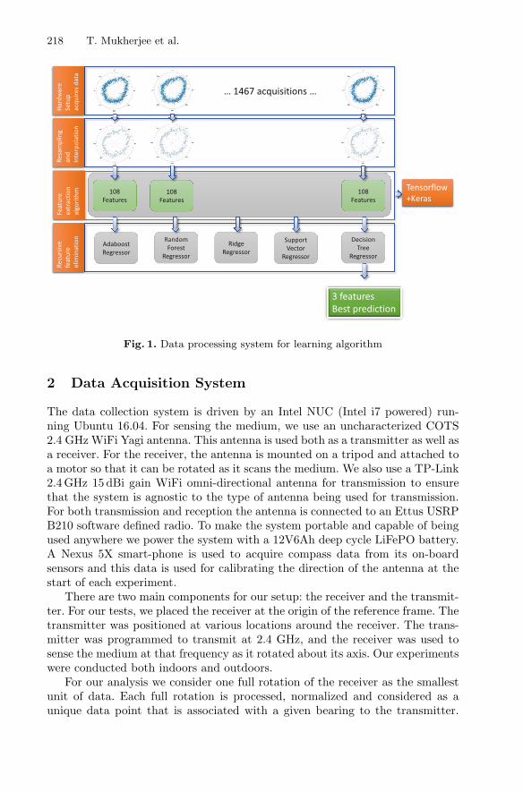
218 T. Mukherjee et al.
Fig. 1. Data processing system for learning algorithm
2 Data Acquisition System
The data collection system is driven by an Intel NUC (Intel i7 powered) run-ning Ubuntu 16.04. For sensing the medium, we use an uncharacterized COTS2.4 GHz WiFi Yagi antenna. This antenna is used both as a transmitter as well asa receiver. For the receiver, the antenna is mounted on a tripod and attached toa motor so that it can be rotated as it scans the medium. We also use a TP-Link2.4 GHz 15 dBi gain WiFi omni-directional antenna for transmission to ensurethat the system is agnostic to the type of antenna being used for transmission.For both transmission and reception the antenna is connected to an Ettus USRPB210 software defined radio. To make the system portable and capable of beingused anywhere we power the system with a 12V6Ah deep cycle LiFePO battery.A Nexus 5X smart-phone is used to acquire compass data from its on-boardsensors and this data is used for calibrating the direction of the antenna at thestart of each experiment.
There are two main components for our setup: the receiver and the transmit-ter. For our tests, we placed the receiver at the origin of the reference frame. Thetransmitter was positioned at various locations around the receiver. The trans-mitter was programmed to transmit at 2.4 GHz, and the receiver was used tosense the medium at that frequency as it rotated about its axis. Our experimentswere conducted both indoors and outdoors.
For our analysis we consider one full rotation of the receiver as the smallestunit of data. Each full rotation is processed, normalized and considered as aunique data point that is associated with a given bearing to the transmitter.
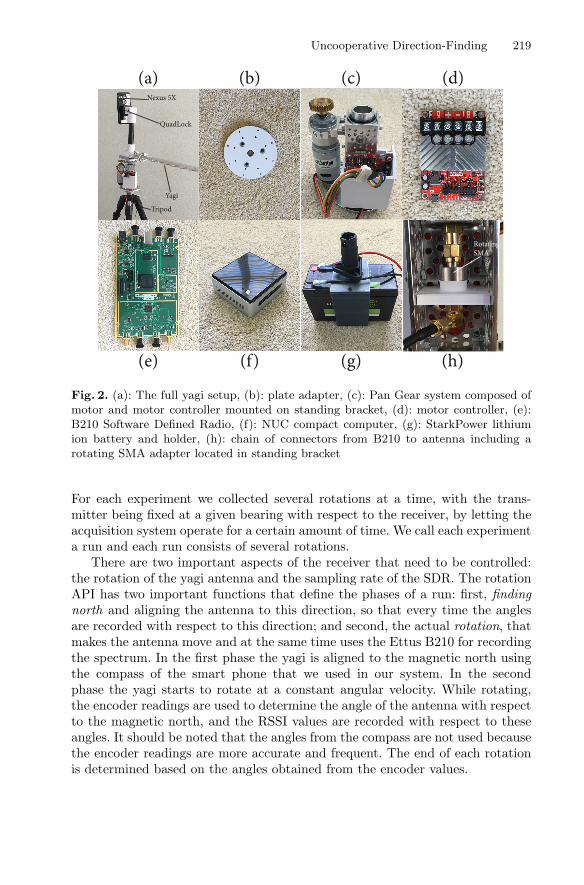
Uncooperative Direction-Finding 219
Fig. 2. (a): The full yagi setup, (b): plate adapter, (c): Pan Gear system composed ofmotor and motor controller mounted on standing bracket, (d): motor controller, (e):B210 Software Defined Radio, (f): NUC compact computer, (g): StarkPower lithiumion battery and holder, (h): chain of connectors from B210 to antenna including arotating SMA adapter located in standing bracket
For each experiment we collected several rotations at a time, with the trans-mitter being fixed at a given bearing with respect to the receiver, by letting theacquisition system operate for a certain amount of time. We call each experimenta run and each run consists of several rotations.
There are two important aspects of the receiver that need to be controlled:the rotation of the yagi antenna and the sampling rate of the SDR. The rotationAPI has two important functions that define the phases of a run: first, findingnorth and aligning the antenna to this direction, so that every time the anglesare recorded with respect to this direction; and second, the actual rotation, thatmakes the antenna move and at the same time uses the Ettus B210 for recordingthe spectrum. In the first phase the yagi is aligned to the magnetic north usingthe compass of the smart phone that we used in our system. In the secondphase the yagi starts to rotate at a constant angular velocity. While rotating,the encoder readings are used to determine the angle of the antenna with respectto the magnetic north, and the RSSI values are recorded with respect to theseangles. It should be noted that the angles from the compass are not used becausethe encoder readings are more accurate and frequent. The end of each rotationis determined based on the angles obtained from the encoder values.
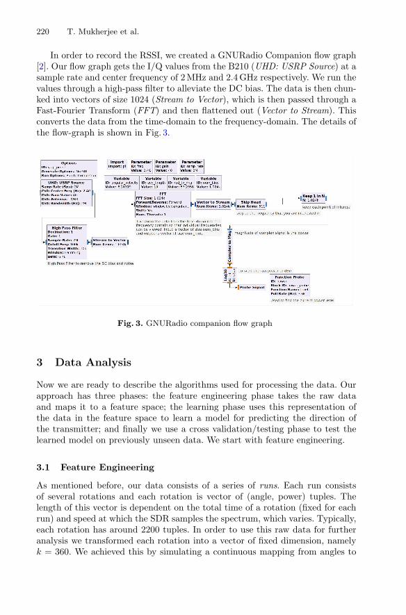
220 T. Mukherjee et al.
In order to record the RSSI, we created a GNURadio Companion flow graph[2]. Our flow graph gets the I/Q values from the B210 (UHD: USRP Source) at asample rate and center frequency of 2 MHz and 2.4 GHz respectively. We run thevalues through a high-pass filter to alleviate the DC bias. The data is then chun-ked into vectors of size 1024 (Stream to Vector), which is then passed through aFast-Fourier Transform (FFT) and then flattened out (Vector to Stream). Thisconverts the data from the time-domain to the frequency-domain. The details ofthe flow-graph is shown in Fig. 3.
Fig. 3. GNURadio companion flow graph
3 Data Analysis
Now we are ready to describe the algorithms used for processing the data. Ourapproach has three phases: the feature engineering phase takes the raw dataand maps it to a feature space; the learning phase uses this representation ofthe data in the feature space to learn a model for predicting the direction ofthe transmitter; and finally we use a cross validation/testing phase to test thelearned model on previously unseen data. We start with feature engineering.
3.1 Feature Engineering
As mentioned before, our data consists of a series of runs. Each run consistsof several rotations and each rotation is vector of (angle, power) tuples. Thelength of this vector is dependent on the total time of a rotation (fixed for eachrun) and speed at which the SDR samples the spectrum, which varies. Typically,each rotation has around 2200 tuples. In order to use this raw data for furtheranalysis we transformed each rotation into a vector of fixed dimension, namelyk = 360. We achieved this by simulating a continuous mapping from angles to

Uncooperative Direction-Finding 221
powers based on the raw data for a single rotation and by reconstructing thevector using this mapping for k evenly spaced points within the range 0 to 2π.The new set of rotation vectors denoted by R is a subset of Rk. For our analysis,we let k = 360 because each run is representative of a sampling from a circle.
Fig. 4. Example rotation withmarkers for the actual angle andtwo predicted angles using the maxRSSI and Decision Tree methods
During the analysis of our data, we noticeda drift in one of the features (moving aver-age max value which is defined below). Thisled us to believe that the encoder measure-ments were changing with time during a run(across rotations). Plotting each run sepa-rately revealed a linear trend with high corre-lation (Fig. 5). In order to correct the drift, wecomputed the least squares regression for themost prominent runs (runs which displayedvery high correlation), averaged the slopesof the resulting lines, and used this value tonegate the drift. The negation step was doneon the raw data for each run because at thestart of each run, the encoder is reset to zero.Once a run is corrected it can be split intorotations. Since each rotation vector can beviewed as a time-series, we use time series fea-ture extraction techniques to map the data into a high dimensional feature space.Feature extraction from time series data is a well studied problem, and we usethe techniques described by Christ et al. [5] to map the data into the featurespace. In all there were 86 features that were extracted using the algorithm. Inaddition to the features extracted using this method, we also added a few othersbased on the idea of a moving average [12].
More precisely, we use the moving average max value, which is the index(angle) in the rotation vector where the max power is observed after applyinga moving average filter. The filter takes a parameter d, the size of the movingaverage which for a given angle is computed by summing the RSSI values corre-sponding to the preceding d angles, the angle itself and the succeeding d angles.Finally this sum is divided by the total number of points (2d+1), which is alwaysodd. We use the moving average max value with filter sizes ranging from 3 to45, using every other integer. This gives an additional 22 features, which bringsthe total to 108 features.
3.2 Learning Algorithms
Note that we want to predict the bearing (direction) of the transmitter withrespect to the receiver for each rotation. As the bearing is a continuous variable,we formulate this as a regression problem. We use several regressors for predictingthe bearing: (1) SVR: Support vector regression is a type of regressor that usesan ε-insensitive loss function to determine the error [17]. We used the RBFkernel and GridSearchCV for optimizing the parameters with cross validation

222 T. Mukherjee et al.
(2) KRR: Kernel ridge regression is similar to SVR but uses a squared-errorloss function [17]. Again, we use the RBF kernel with GridSearchCV to get theoptimal parameter (3) Decision Tree [3]: we used a max depth of 4 for our modeland finally (4) AdaBoost with Decision Tree [7,26]: short for adaptive boosting,uses another learning algorithm as a “weak learner”. We used a decision treewith max depth 4 as our “weak learner”.
Although we have a total of 108 features, not all of them will be important forprediction purposes. As a result, we try two different approaches for selectingthe most useful features: (1) the first one ranks each feature through a scor-ing function, and (2) the second prunes features at each iteration and is calledrecursive feature extraction with cross-validation [11]. For the first we use thefunction SelectKBest, and for the later we used RFECV , both implementedin ScikitLearn.
We also use neural networks for the prediction task. We used Keras for ourexperiments, which is a high-level neural networks API, written in Python andcapable of running on top of TensorFlow. We used the Sequential model inKeras, which is a linear stack of layers. The results on our dataset are describedin Sect. 4.
4 Experiments and Results
In this section we present the results of our experiments. In total, we collected1467 rotations (after drift correction) at 76 unique angles (an example of a rota-tion reduced to 360 vertices can be seen in Fig. 4). After reducing each rotationto 360 power values, we ran the dataset through the feature extractor, which pro-duced 108 total features. We tried out several regressors, namely, (SVR, KR, DT,and AB) and strategies:- (moving average max value without learning, movingaverage max value with learning, SelectKBest, RFECV, and neural networks).The objective for this set of tests was to find the predictor that yielded the lowestmean absolute error (MAE), which is the average of the absolute value of eacherror from that test.
4.1 Regressors
We used the data from the feature selection phase to test a few regressors. Foreach regressor, we split the data (50% train, 50% test), trained and tested themodel, and calculated the MAE. We ran this 100 times for each regressor andtook the overall average to show which regressor preformed the best with all thefeatures. The results from these tests are in Table 1.
From the results we can see that decision trees give the lowest MAE comparedto the other regressors. We also noticed that decision trees ran the train/testcycle much faster than any other regressor. Based on these results, we decidedto use the decision tree regressor for the rest of our tests.
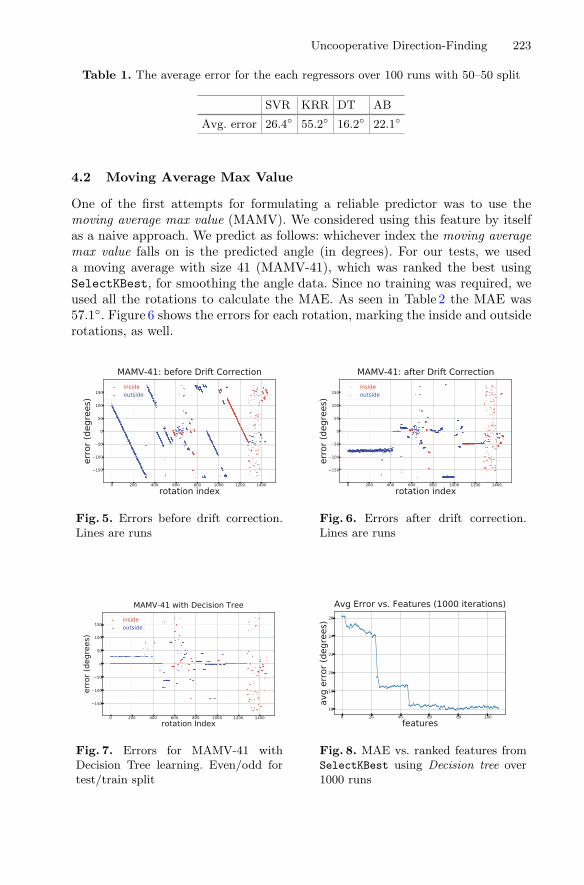
Uncooperative Direction-Finding 223
Table 1. The average error for the each regressors over 100 runs with 50–50 split
SVR KRR DT AB
Avg. error 26.4◦ 55.2◦ 16.2◦ 22.1◦
4.2 Moving Average Max Value
One of the first attempts for formulating a reliable predictor was to use themoving average max value (MAMV). We considered using this feature by itselfas a naive approach. We predict as follows: whichever index the moving averagemax value falls on is the predicted angle (in degrees). For our tests, we useda moving average with size 41 (MAMV-41), which was ranked the best usingSelectKBest, for smoothing the angle data. Since no training was required, weused all the rotations to calculate the MAE. As seen in Table 2 the MAE was57.1◦. Figure 6 shows the errors for each rotation, marking the inside and outsiderotations, as well.
Fig. 5. Errors before drift correction.Lines are runs
Fig. 6. Errors after drift correction.Lines are runs
Fig. 7. Errors for MAMV-41 withDecision Tree learning. Even/odd fortest/train split
Fig. 8. MAE vs. ranked features fromSelectKBest using Decision tree over1000 runs

224 T. Mukherjee et al.
Our next step was to use the decision trees with the MAMV-41 feature. Weapplied a 50/50 train/test split in the data and calculated the MAE for each run.We averaged and reported the MAE for all runs. The average MAE over 1000runs was 25.9◦ (Table 2). Figure 7 shows a graph of errors for the train/test splitwhere the odd index rotations were for training and the even index rotationswere for testing.
4.3 SelectKBest
As mentioned before, we used SelectKBest to rank all the features. In order toget stable rankings, we ran this 100 times and averaged those ranks. Once we hadthe ranked list of features, we created a “feature profile” by iteratively addingthe next best feature, running train/test with the decision tree regressor for thatset of features, and recording the MAE. We repeated this process 1000 times andthe results are shown in (Fig. 8). It is to be noted that the error does not changeconsiderably for a large number of consecutive features but there are steep dropsin the error around certain features. This is because many features are similarand using them for the prediction task does not change the error significantly.The first plateau consists mostly of MAMV features since they were ranked thebest among all the other features. The first major drop is at ranked feature 24,which marks the start of the set of continuous wavelet transform coefficients(CWT). The second major drop is cause by the addition of the 2nd coefficientfrom Welch’s transformation [24] (2-WT) at ranked feature 46. Beyond that, nosignificant decrease in MAE is achieved by the inclusion of another feature. Thebest average MAE over the whole profile is 15.7◦ at 78 features (Table 2).
4.4 RFECV and Neural Network
We ran RFECV with a decision tree regressor using a different random state everytime. RFECV consistently returned three features: MAMV-23, MAMV-41, and2-WT. Using these three features, we trained and tested on the data with a50/50 split 10000 times with the decision tree regressor. The average MAE was11.0◦ (Table 2). Between RFECV and SelectKBest, there are four unique featureswhich stand out among the rest. To be thorough, we found the average MAE forall groups of three and four from these four features. None of them were betterthan the original three features from RFECV.
Table 2. Comparison of average error among predictor methods
MAMV-41 MAMV-41 (DT) SelectKBest RFECV Neural net
Avg. MAE ±57.1◦ ±25.9◦ ±15.7◦ ±11.0◦ ±15.7◦
For the neural network approach, we used all the features which were pro-duced from the feature selection phase. We settled on a 108 ⇒ 32 ⇒ 4 ⇒ 1
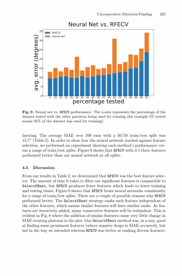
Uncooperative Direction-Finding 225
Fig. 9. Neural net vs. RFECV performance. The x-axis represents the percentage of thedataset tested with the other partition being used for training (for example 5% testedmeans 95% of the dataset was used for training).
layering. The average MAE over 100 runs with a 50/50 train/test split was15.7◦ (Table 2). In order to show how the neural network stacked against featureselection, we performed an experiment showing each method’s performance ver-sus a range of train/test splits. Figure 9 shows that RFECV with it’s three featuresperformed better than our neural network at all splits.
4.5 Discussion
From our results in Table 2, we determined that RFECV was the best feature selec-tor. The amount of time it takes to filter out significant features is comparable toSelectKBest, but RFECV produces fewer features which leads to lower trainingand testing times. Figure 9 shows that RFECV beats neural networks consistentlyfor a range of train/test splits. There are a couple of possible reasons why RFECVperformed better. The SelectKBest strategy ranks each feature independent ofthe other features, which means similar features will have similar ranks. As fea-tures are iteratively added, many consecutive features will be redundant. This isevident in Fig. 8 where the addition of similar features cause very little change inMAE creating plateaus in the plot. Our SelectKBest method was, in a way, goodat finding some prominent features (where massive drops in MAE occurred), butnot in the way we intended whereas RFECV was better at ranking diverse features.
226 T. Mukherjee et al.
5 Conclusion and Future Work
The main contribution of this paper is to show that using pure data miningtechniques with the RSSI values, one can achieve good accuracies in direction-finding using COTS directional receivers. There are several directions that canbe pursued for future work: (1) How accurately can cell phones locations beanalyzed with the current setup? (2) Can we minimize the total size of ourreceive system? (3) How well does this system work for different frequenciesand ranges around them? (4) When used in a distributed setting, how muchaccuracy can one achieve for localization, given k receivers operating at the sametime (assuming the distances between them is known). In the journal version ofthis paper, we will show how to theoretically solve this problem, but extensiveexperimental results are lacking. In the near future, we plan to pursue some ofthese questions using our existing hardware setup.
References
1. Bahl, V., Padmanabhan, V.: RADAR: an in-building RF-based user loca-tion and tracking system. Institute of Electrical and Electronics Engineers,Inc., March 2000. https://www.microsoft.com/en-us/research/publication/radar-an-in-building-rf-based-user-location-and-tracking-system/
2. Blossom, E.: GNU radio: tools for exploring the radio frequency spectrum. LinuxJ. 2004(122), 4 (2004). http://dl.acm.org/citation.cfm?id=993247.993251
3. Breiman, L., Friedman, J., Olshen, R., Stone, C.: Classification and RegressionTrees. Wadsworth, Belmont (1984)
4. Capkun, S., Hamdi, M., Hubaux, J.P.: GPS-free positioning in mobile ad hoc net-works. Clust. Comput. 5(2), 157–167 (2002)
5. Christ, M., Kempa-Liehr, A.W., Feindt, M.: Distributed and parallel timeseries feature extraction for industrial big data applications. arXiv preprintarXiv:1610.07717 (2016)
6. Finders, D.: Introduction into theory of direction finding (2017). http://telekomunikacije.etf.bg.ac.rs/predmeti/ot3tm2/nastava/df.pdf. Accessed 28 Feb2017
7. Freund, Y., Schapire, R.E.: A decision-theoretic linearization of on-line learningand an application to boosting (1995)
8. Gething, P.: Radio Direction-Finding: And the Resolution of MulticomponentWave-Fields. IEE Electromagnetic Waves Series. Peter Peregrinus, London (1978).https://books.google.com/books?id=BCcIAQAAIAAJ
9. Graefenstein, J., Albert, A., Biber, P., Schilling, A.: Wireless node localizationbased on RSSI using a rotating antenna on a mobile robot. In: 2009 6th Workshopon Positioning, Navigation and Communication, pp. 253–259, March 2009
10. Graefenstein, J., Albert, A., Biber, P., Schilling, A.: Wireless node localizationbased on RSSI using a rotating antenna on a mobile robot. In: 6th Workshop onPositioning, Navigation and Communication (WPNC 2009), pp. 253–259. IEEE(2009)
11. Guyon, I., Weston, J., Barnhill, S., Vapnik, V.: Gene selection for cancer classifi-cation using support vector machines. Mach. Learn. 46, 389–422 (2002)

Uncooperative Direction-Finding 227
12. Hamilton, J.D.: Time Series Analysis, vol. 2. Princeton University Press, Princeton(1994)
13. Huang, W., Xiong, Y., Li, X.Y., Lin, H., Mao, X., Yang, P., Liu, Y., Wang,X.: Swadloon: direction finding and indoor localization using acoustic signal byshaking smartphones. IEEE Trans. Mob. Comput. 14(10), 2145–2157 (2015).http://dx.doi.org/10.1109/TMC.2014.2377717
14. Ito, S., Kawaguchi, N.: Orientation estimation method using divergence of signalstrength distribution. In: Third International Conference on Networked SensingSystems, pp. 180–187 (2006)
15. Kolster, F.A., Dunmore, F.W.: The radio direction finder and its application tonavigation, Washington (1922). ISBN: 978-1-333-95286-0
16. Moell, J., Curlee, T.: Transmitter Hunting: Radio Direction Finding Simpli-fied. TAB Book, McGraw-Hill Education (1987). https://books.google.com/books?id=RfzF2-fHJ6MC
17. Murphy, K.P.: Machine Learning: A Probabilistic Perspective. MIT Press,Cambridge (2012)
18. Porat, B., Friedlander, B.: Direction finding algorithms based on high-order statis-tics. IEEE Trans. Signal Process. 39(9), 2016–2024 (1991)
19. Roy, R., Kailath, T.: ESPRIT-estimation of signal parameters via rotational invari-ance techniques. IEEE Trans. Acoust. Speech Signal Process. 37(7), 984–995 (1989)
20. Satoh, H., Ito, S., Kawaguchi, N.: Position estimation of wireless access pointusing directional antennas. In: Strang, T., Linnhoff-Popien, C. (eds.) LoCA 2005.LNCS, vol. 3479, pp. 144–156. Springer, Heidelberg (2005). https://doi.org/10.1007/11426646 14
21. Savarese, C., Rabaey, J.M., Beutel, J.: Location in distributed ad-hoc wireless sen-sor networks. In: Proceedings of the IEEE International Conference on Acoustics,Speech, and Signal Processing (ICASSP 2001), vol. 4, pp. 2037–2040. IEEE (2001)
22. Schmidt, R.: Multiple emitter location and signal parameter estimation. IEEETrans. Antennas Propag. 34(3), 276–280 (1986)
23. Ward, T., Pasiliao, E.L., Shea, J.M., Wong, T.F.: Autonomous navigation to anRF source in multipath environments. In: 2016 IEEE Military CommunicationsConference (MILCOM 2016), pp. 186–191, November 2016
24. Welch, P.: The use of fast fourier transform for the estimation of power spectra: amethod based on time averaging over short, modified periodograms. IEEE Trans.Audio Electroacoust. 15(2), 70–73 (1967)
25. Wikipedia: Direction finding – Wikipedia, the free encyclopedia (2016). https://en.wikipedia.org/wiki/Direction finding. Accessed 20 Dec 2016
26. Zhu, J., Zou, H., Rosset, S., Hastie, T.: Mutli-class AdaBoost (2009)27. Zhuo, L., Dan, S., Yougang, G., Yaqin, S., Junjian, B., Zhiliang, T.: The distinction
among electromagnetic radiation source models based on directivity with supportvector machines. In: 2014 International Symposium on Electromagnetic Compati-bility, Tokyo (EMC 2014/Tokyo), pp. 617–620. IEEE (2014)
Sequential Keystroke Behavioral Biometricsfor Mobile User Identification via Multi-view
Deep Learning
Lichao Sun1(B), Yuqi Wang3, Bokai Cao1, Philip S. Yu1, Witawas Srisa-an2,and Alex D. Leow1
1 University of Illinois at Chicago, Chicago, IL 60607, USA{lsun29,caobokai,psyu}@uic.edu, [email protected] University of Nebraska–Lincoln, Lincoln, NE 68588, USA
[email protected] Hong Kong Polytechnic University, Kowloon, Hong Kong
Abstract. With the rapid growth in smartphone usage, more organiza-tions begin to focus on providing better services for mobile users. Useridentification can help these organizations to identify their customersand then cater services that have been customized for them. Currently,the use of cookies is the most common form to identify users. However,cookies are not easily transportable (e.g., when a user uses a differentlogin account, cookies do not follow the user). This limitation motivatesthe need to use behavior biometric for user identification. In this paper,we propose DeepService, a new technique that can identify mobile usersbased on user’s keystroke information captured by a special keyboard orweb browser. Our evaluation results indicate that DeepService is highlyaccurate in identifying mobile users (over 93% accuracy). The techniqueis also efficient and only takes less than 1 ms to perform identification.
1 Introduction
Smart mobile devices are now an integral part of daily life; they are our maininterface to cyber-world. We use them for on-line shopping, education, entertain-ment, and financial transactions. As such, it is not surprising that companies areworking hard to improve their mobile services to gain competitive advantages.Accurately and non-intrusively identifying users across applications and devicesis one of the building blocks for better mobile experiences, since not only com-panies can attract users based on their characteristics from various perspectives,but also users can enjoy the personalized services without much effort [15].
User identification is a fundamental, but yet an open problem in mobile com-puting. Traditional approaches resort to user account information or browsinghistory. However, such information can pose security and privacy risks, and itis not robust as can be easily changed, e.g., the user changes to a new deviceor using a different application. Monitoring biometric information including ac© Springer International Publishing AG 2017Y. Altun et al. (Eds.): ECML PKDD 2017, Part III, LNAI 10536, pp. 228–240, 2017.https://doi.org/10.1007/978-3-319-71273-4_19

Sequential Keystroke Behavioral Biometrics for Mobile User Identification 229
user’s typing behaviors tends to produce consistent results over time while beingless disruptive to user’s experience. Furthermore, there are different kinds ofsensors on mobile devices, meaning rich biometric information of users can besimultaneously collected. Thus, monitoring biometric information appears to bequite promising for mobile user identification.
To date, only a few studies have utilized biometric information for mobileuser identification on web browser [1,19]. Important questions such as what kindof biometric information can be used, how does one capture user characteristicsfrom the biometric, and what accuracy of the mobile user identification can beachieved, are largely unexplored. Although there are some researches on mobileuser authentication through biometrics [8,20], authentication is a simplified ver-sion of identification, and directly employing authentication would either beinfeasible or lead to low accuracy. This work focuses on mobile user identifica-tion, and could also be applied to authentication.
In this paper, we collect information from basic keystroke and the accelerom-eter on the phone, and then propose DeepService, a multi-view deep learningmethod, to utilize this information. To the best of our knowledge, this is the firsttime multi-view deep learning is applied to mobile user identification. Throughseveral empirical experiments, we showed that the proposed method is able tocapture the user characteristics and identify users with high accuracy.
Our contributions are summarized as follows.
1. We propose DeepService, a multi-view deep learning method, to utilize easyto collect user biometrics for accurate user identification.
2. We conduct several experiments to demonstrate the effectiveness and superi-ority of the proposed method against various baseline methods.
3. We give several analyses and insights through the experiments.
The rest of this paper is organized as follows. Section 2 provides backgroundinformation on deep learning, and reviews prior research efforts related to thiswork. Section 3 introduces DeepService and describes the design and imple-mentation details. Section 4 reports the results of our empirical evaluation onthe performance of DeepService with respect to other learning techniques.The last section concludes this work and discusses future work.
2 Background and Related Work
In this section, we provide additional background information on deep learningstructure, and review prior research efforts related to our proposed work.
2.1 Background on Deep Learning Structure
Deep learning is a branch of machine learning based on a set of algorithmsthat attempt to model high level abstractions in data, which is also called deepstructured learning, deep neural network learning or deep machine learning.Deep learning is a concept and a framework instead of a particular method.
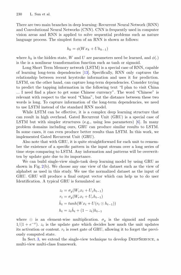
230 L. Sun et al.
There are two main branches in deep learning: Recurrent Neural Network (RNN)and Convolutional Neural Networks (CNN). CNN is frequently used in computervision areas and RNN is applied to solve sequential problems such as naturelanguage process. The simplest form of an RNN is shown as follows:
hk = φ(Wxk + Uhk−1)
where hk is the hidden state, W and U are parameters need be learned, and φ(.)is the is a nonlinear transformation function such as tanh or sigmoid.
Long Short Term Memory network (LSTM) is a special case of RNN, capableof learning long-term dependencies [13]. Specifically, RNN only captures therelationship between recent keystroke information and uses it for prediction.LSTM, on the other hand, can capture long-term dependencies. Consider tryingto predict the tapping information in the following text “I plan to visit China... I need find a place to get some Chinese currency”. The word “Chinese” isrelevant with respect to the word “China”, but the distance between these twowords is long. To capture information of the long-term dependencies, we needto use LSTM instead of the standard RNN model.
While LSTM can be effective, it is a complex deep learning structure thatcan result in high overhead. Gated Recurrent Unit (GRU) is a special case ofLSTM but with simpler structures (e.g., using less parameters) [6]. In manyproblem domains including ours, GRU can produce similar results to LSTM.In some cases, it can even produce better results than LSTM. In this work, weimplemented Gated Recurrent Unit (GRU).
Also note that with GRU, it is quite straightforward for each unit to remem-ber the existence of a specific pattern in the input stream over a long series oftime steps comparing to LSTM. Any information and patterns will be overwrit-ten by update gate due to its importance.
We can build single-view single-task deep learning model by using GRU asshown in Fig. 2(b). We choose any one view of the dataset such as the view ofalphabet as used in this study. We use the normalized dataset as the input ofGRU. GRU will produce a final output vector which can help us to do userIdentification. A typical GRU is formulated as:
zt = σg(Wzxt + Uzht−1)rt = σg(Wrxt + Urht−1)
ht = tanh(Wxt + U(rt � ht−1))
ht = ztht + (1 − zt)ht−1
where � is an element-wise multiplication. σg is the sigmoid and equals1/(1 + e−x). zt is the update gate which decides how much the unit updatesits activation or content. rt is reset gate of GRU, allowing it to forget the previ-ously computed state.
In Sect. 3, we extend the single-view technique to develop DeepService, amulti-view multi-class framework.

Sequential Keystroke Behavioral Biometrics for Mobile User Identification 231
2.2 Related Work
Most previous works focus on user authorization, rather than identification,based on biometrics. For example, there are multiple approaches to get physio-logical information that include facial features and iris features [7,9]. This phys-iological information can also be used for identification, but it requires extrapermission from the users. Our method uses behavioral biometrics to identifythe users without any cookies or other personal information.
Recently, more research work on continuous authorization problem hasemerged for mobile users. Some prior efforts also focus on studying touchscreengestures [20] or behavioral biometric behaviors such as reading, walking, drivingand tapping [3,4]. There are research efforts focusing on offering better securityservices for mobile users. However, their security models have to be installed onthe mobile devices. They then perform binary classifications to detect unautho-rized behaviors. Our work focuses on building a general user identification model,which can also be deployed on the web, local devices or even network routers.Our work also focuses on improving users’ experience through customized ser-vices including providing recommendations and relevant advertisements.
Recently, some research groups focus on mobile user identification based onweb browsing information [1,19]. Abramson and Gore try to identify users’ webbrowsing behaviors by analyzing cookies information. However, our model hasbeen designed to target harder problems without using trail of information suchas cookies or browsing history. We, instead, use behavioral biometrics to iden-tify users. Information needed can be easily collected from web browser usingJavascript.
3 DeepService: A Multi-view Multi-class Frameworkfor User Identification on Mobile Devices
DeepService is a multi-view and multi-class identification framework via adeep structure. It contains three main steps to identify each user from severalusers. This process is shown in Fig. 1 and summarized below:
1. In the first step, we collect sequential tapping information and accelerometerinformation from 40 volunteers who have used our provided smartphones for8 weeks. We retrieve such sequential data in a real-time manner.
2. In the second step, we prepare the collected information as multi-view datafor the problem of user identification.
3. In the third step, we model the multi-view data via a deep structure toperform multi-class learning.
4. In the last step, we compare the performance of the proposed approach withthe traditional machine learning techniques for multi-class identification suchas support vector machine and random forest. This step is discussed in Sect. 4.
Next, we describe each of the first three steps in turn.

232 L. Sun et al.
Fig. 1. Framework of DeepService
3.1 Data Collection
First, we describe the data collection process. Our study involves 40 volunteers.The main selection criterion is based on their prior experience with using smart-phones. All selected candidates have used smartphones for at least 11 years (somehave used smartphones for 18 years). In terms of age, the youngest participantis 30 years old and the oldest one is 63 years old.
Each volunteer was given a same smartphone with the custom software key-board. Out of the 40 volunteers, we find that 26 of them (17 females and 9 males)have used the provided phones at least 20 times in 8 weeks. The data generatedby these 26 volunteers is the one we ended up using in this study. The most activeparticipant has used the phone 4702 times while the least active participant hasused the phone only 29 times.
3.2 Data Processing
When users type on the smartphone keyboard either locally or on a webbrowser, our custom keyboard would collect the meta-information associatedwith the users’ typing behaviors, including duration of a keystroke, time sincelast keystroke, and distance from last keystroke, as well as the accelerometervalues along three directions. Due to privacy concerns, the actual characterstyped by users are not collected. However, we do collect the categorical informa-tion of each keystroke, e.g., alphanumeric characters, special characters, space,backspace. Note that such information can easily be collected from web browserusing Javascript as well.
In the data collection process, there are inevitable missing data. For example,when the first time a user uses the phone, the feature time since last key isundefined. We replace these missing values with 0. After the complement ofmissing values, we normalize all the features to the range of [0, 1].
A typical usage of keyboard would likely result in a session consisting morethan one keystroke. For example, a simple message such as “How are you?”

Sequential Keystroke Behavioral Biometrics for Mobile User Identification 233
involves sequential keystrokes as well as multiple types of inputs (alphabets andspecial characters). In this study, one instance represents one usage session ofthe phone by the user. A session instance sij represents the j-th session of thei-th user in the data set, which consists of three different types of sequentialdata. Let’s denote sij = {c
(1)ij , c
(2)ij , c
(3)ij } where c
(1)ij is the time series of alphabet
keystrokes, c(2)ij is the time series of special character keystrokes, and c
(3)ij is the
time series of accelerometer values. It is difficult to align the sequential featuresin different views because of different timestamps and sampling rates. For exam-ple, accelerometer values are much denser than special character keystrokes.Therefore, it is intuitive to treat c
(1)ij , c
(2)ij , and c
(3)ij as multi-view time series that
together compose the complementary information for user identification.
3.3 Multi-view Multi-class Deep Learning (MVMC)
Now, we discuss the approach to apply deep learning for constructing the useridentification model. The approach is based on Multi-view Multi-class (MVMC)learning with a deep structure.
As mentioned previously, we employ three different views. Each view Vi con-tains different number of features and different number of samples. In Fig. 2(a),we can use fusion method to combine datasets of different views. However, due tothe different number of features, and the number of records in each view of eachsession, it is hard to build a single-view dataset from many other views. Hence,instead of concatenating different views into one view, we choose to use themseparately. This is done to avoid losing information as in the case when multipleviews are combined to create a view. One major information that we want topreserve is the sequence of keystrokes. By using multi-view, we are able to main-tain each view separately but then use multiple views to make predictions [5,17].Recently, various methods have been proposed for this purpose [10–12].
Fig. 2. A comparison of different frameworks of learning models: left: (a) traditionallearning methods; middle (b) single-view multi-class; (c) multi-view multi-class

234 L. Sun et al.
Before we generate multi-view multi-class learning, we first create single-view multi-class learning as shown in Fig. 2(b) (previously discussed in Sect. 2).Through that model, we can prove the multi-view can help us to improve theperformance for identification and we can determine which view most contributesto the identification process. First, we separate the data set into multiple views.In this case, we have a view of alphabets, a view of numbers and symbols, anda view of tapping acceleration. Then, we use GRU and Bidirectional RecurrentNeural Network (we refer to the combination of these two approaches as GRU-BRNN) to build the hidden layers for each view. In the output layer, we usesoftmax function to perform multiple classifications. Finally, we can evaluatethe performance on each view.
We describe the framework that uses multi-view and multi-class learningwith deep structure in Fig. 2(c). Comparing to single-view multi-class, multi-view multi-class is a more general model. After we use GRU-BRNN to build thehidden layers for each view. We then concatenate the last layer information fromeach GRU-BRNN model of each view. We use the last concatenated layer, whichcontains all information from different views, for identification.
As GRU extracts a latent feature representation out of each time series, thenotions of sequence length and sampling time points are removed from the latentspace. This avoids the problem of dealing directly with the heterogeneity of thetime series from each view. The difference between multi-view multi-class andsingle-view multi-class learning is that we use the multiple views of the datasetand we use the latent information of each view for prediction, which can improveperformance over using only a single-view dataset. We can consider single-viewmulti-class as a special case of multi-view multi-class learning.
Note that in deep learning, different optimization functions can greatly influ-ence the training speed and the final performance. There are several optimizerssuch as RMSprop and Adam [16]. In this work, we use an improved versionof Adam called Nesterov Adam (Nadam) which is a RMSprop with Nesterovmomentum.
4 Experiment
To examine the performance of the proposed DeepService on identifying mobileusers. Our experiments were done on a large-scale real-world data set. We alsocompared the results with those from several state-of-the-art shallow machinelearning methods. In this section, we describe how we conducted our experi-ments. We then present the experimental results and analysis.
4.1 Baselines: Keystroke-Based Behavior Biometric Methodsfor Continuous Identification
In previous work on keystroke-based continuous identification with machine learn-ing techniques [2,4,14], Support Vector Machine, Decision Tree, and RandomForest are widely used for continuous identification.

Sequential Keystroke Behavioral Biometrics for Mobile User Identification 235
Logistic Regression (LR): LR is a linear model with sigmoid function for clas-sification. It is an efficient algorithm which can handle both dense and sparseinput.
Linear Support Vector Machine (LSVM): LSVM is widely used in many previousauthorization and identification works [2,4,14]. LSVM is a linear model that findsthe best hyperplane by maximizing the margin between multiple classes.
Random Forest/Decision Tree: Other learning methods such as Random Forestand Decision Tree have not yet been adopted in many behavior biometric workfor continuous identification by keystrokes information only. However, DecisionTree is a interpretable classification model for binary classification. It is a treestructure, and features form patterns are nodes in the tree. Random Forest isan ensemble learning method for classification that builds many decision treesduring training and combines their outputs for the final prediction. Previouswork [18] shows that tree structure methods can work more efficiently thanSVM, and can do better binary classification comparing to SVM. We use differenttraditional learning methods on our data set as the baselines.
4.2 Evaluation of DeepService Framework
Since the number of session usage for every user is different, we use four per-formance measures to evaluate unbalanced results: Recall, Precision F1 Score(F-Measure), and Accuracy. They are defined as:
Recall =TP
TP + FNF1 =
2 ∗ Precision ∗ Recall
Precision + Recall
Precision =TN
TN + FPAccuracy =
TP + TN
TP + TN + FP + FN
Next, we report the performance of DeepService using our data set. Wemeasured precision, recall and accuracy, f1 score (f-measure) for different models.Based on the results, we can make the following conclusions.
– DeepService can identify between two known people at almost 100% accu-racy in our experiment. This proves that our data set contains valuable bio-metric information to distinguish and identify users.
– DeepService can do identification with only acceleration records, even whenuser is not using the keyboard.
– DeepService is effective at identifying a large number of users simultane-ously either locally or on a web browser.
4.3 User Pattern Analysis
In this section, we evaluate the feature patterns for different users. In Fig. 3, weshows the feature patterns analysis of top 5 active users in multi-view.
In the view of Alphabet graphs, each user tends to have unique patterns withrespect to the duration, the time since last key, and the number of keystrokes in
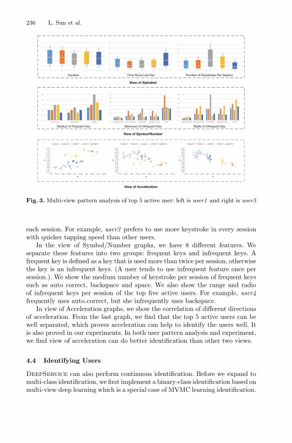
236 L. Sun et al.
Fig. 3. Multi-view pattern analysis of top 5 active user: left is user1 and right is user5
each session. For example, user3 prefers to use more keystroke in every sessionwith quicker tapping speed than other users.
In the view of Symbol/Number graphs, we have 8 different features. Weseparate these features into two groups: frequent keys and infrequent keys. Afrequent key is defined as a key that is used more than twice per session, otherwisethe key is an infrequent keys. (A user tends to use infrequent feature once persession.). We show the medium number of keystroke per session of frequent keyssuch as auto correct, backspace and space. We also show the range and radioof infrequent keys per session of the top five active users. For example, user4frequently uses auto correct, but she infrequently uses backspace.
In view of Acceleration graphs, we show the correlation of different directionsof acceleration. From the last graph, we find that the top 5 active users can bewell separated, which proves acceleration can help to identify the users well. Itis also proved in our experiments. In both user pattern analysis and experiment,we find view of acceleration can do better identification than other two views.
4.4 Identifying Users
DeepService can also perform continuous identification. Before we expand tomulti-class identification, we first implement a binary-class identification based onmulti-view deep learning which is a special case of MVMC learning identification.
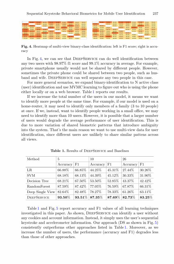
Sequential Keystroke Behavioral Biometrics for Mobile User Identification 237
Fig. 4. Heatmap of multi-view binary-class identification: left is F1 score; right is accu-racy
In Fig. 4, we can see that DeepService can do well identification betweenany two users with 98.97% f1 score and 99.1% accuracy in average. For example,private smartphone usually would not be shared by different people. However,sometimes the private phone could be shared between two people, such as hus-band and wife. DeepService can well separate any two people in this case.
For more general scenarios, we expand binary-identification to N active class(user) identification and use MVMC learning to figure out who is using the phoneeither locally or on a web browser. Table 1 reports our results.
If we increase the total number of the users in our model, it means we wantto identify more people at the same time. For example, if our model is used on ahome-router, it may need to identify only members of a family (3 to 10 people)at once. If we, instead, want to identify people working in a small office, we mayneed to identify more than 10 users. However, it is possible that a larger numberof users would degrade the average performance of user identification. This isdue to more variation of shared biometric patterns that introduce ambiguityinto the system. That’s the main reason we want to use multi-view data for useridentification, since different users are unlikely to share similar pattens acrossall views.
Table 1. Results of DeepService and Baselines
Method 5 10 26
Accuracy F1 Accuracy F1 Accuracy F1
LR 66.88% 66.85% 44.25% 45.31% 27.44% 30.26%
SVM 68.18% 68.13% 44.39% 45.12% 30.33% 31.90%
Decision Tree 68.21% 67.50% 53.50% 52.85% 43.37% 42.42%
RandomForest 87.59% 87.42% 77.05% 76.59% 67.87% 66.31%
Deep Single View 82.64% 82.48% 78.27% 78.33% 61.26% 63.11%
DeepService 93.50% 93.51% 87.35% 87.69% 82.73% 83.25%
Table 1 and Fig. 5 report accuracy and F1 values of all learning techniquesinvestigated in this paper. As shown, DeepService can identify a user withoutany cookies and account information. Instead, it simply uses the user’s sequentialkeystroke and accelerometer information. Our approach (DS as shown in Fig. 5)consistently outperforms other approaches listed in Table 1. Moreover, as weincrease the number of users, the performance (accuracy and F1) degrades lessthan those of other approaches.
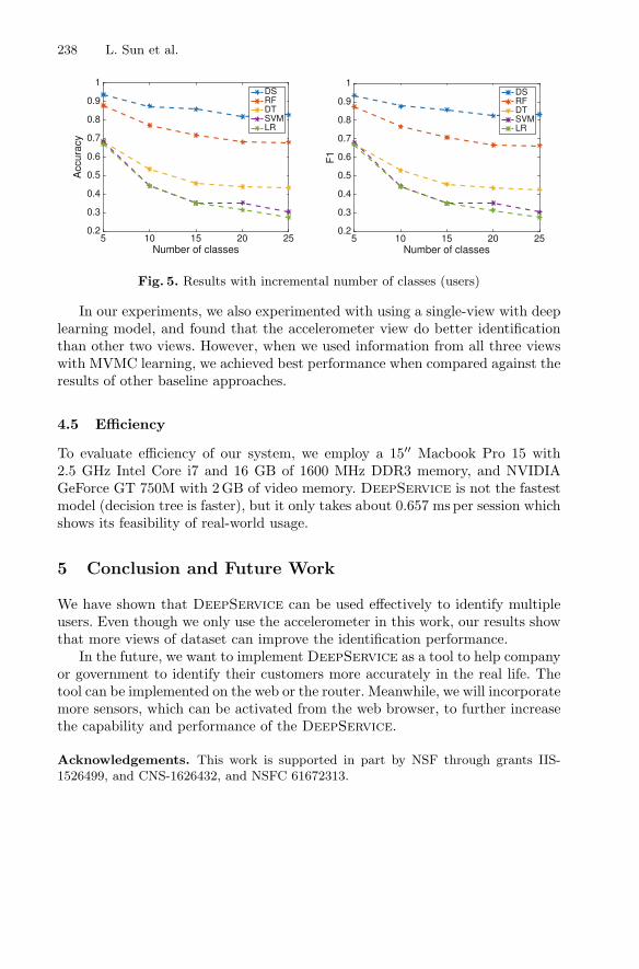
238 L. Sun et al.
Fig. 5. Results with incremental number of classes (users)
In our experiments, we also experimented with using a single-view with deeplearning model, and found that the accelerometer view do better identificationthan other two views. However, when we used information from all three viewswith MVMC learning, we achieved best performance when compared against theresults of other baseline approaches.
4.5 Efficiency
To evaluate efficiency of our system, we employ a 15′′ Macbook Pro 15 with2.5 GHz Intel Core i7 and 16 GB of 1600 MHz DDR3 memory, and NVIDIAGeForce GT 750M with 2 GB of video memory. DeepService is not the fastestmodel (decision tree is faster), but it only takes about 0.657 ms per session whichshows its feasibility of real-world usage.
5 Conclusion and Future Work
We have shown that DeepService can be used effectively to identify multipleusers. Even though we only use the accelerometer in this work, our results showthat more views of dataset can improve the identification performance.
In the future, we want to implement DeepService as a tool to help companyor government to identify their customers more accurately in the real life. Thetool can be implemented on the web or the router. Meanwhile, we will incorporatemore sensors, which can be activated from the web browser, to further increasethe capability and performance of the DeepService.
Acknowledgements. This work is supported in part by NSF through grants IIS-1526499, and CNS-1626432, and NSFC 61672313.
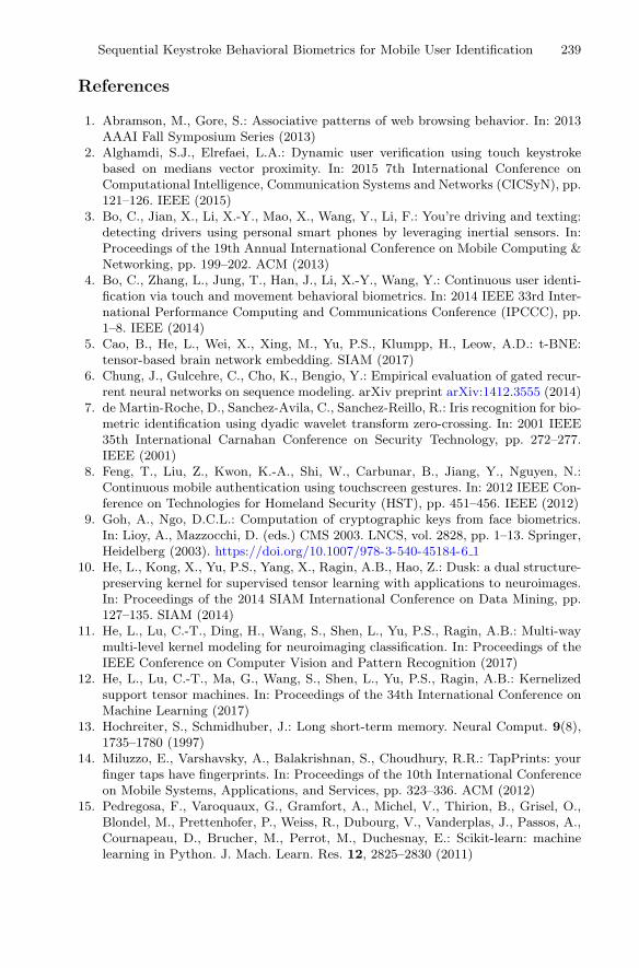
Sequential Keystroke Behavioral Biometrics for Mobile User Identification 239
References
1. Abramson, M., Gore, S.: Associative patterns of web browsing behavior. In: 2013AAAI Fall Symposium Series (2013)
2. Alghamdi, S.J., Elrefaei, L.A.: Dynamic user verification using touch keystrokebased on medians vector proximity. In: 2015 7th International Conference onComputational Intelligence, Communication Systems and Networks (CICSyN), pp.121–126. IEEE (2015)
3. Bo, C., Jian, X., Li, X.-Y., Mao, X., Wang, Y., Li, F.: You’re driving and texting:detecting drivers using personal smart phones by leveraging inertial sensors. In:Proceedings of the 19th Annual International Conference on Mobile Computing &Networking, pp. 199–202. ACM (2013)
4. Bo, C., Zhang, L., Jung, T., Han, J., Li, X.-Y., Wang, Y.: Continuous user identi-fication via touch and movement behavioral biometrics. In: 2014 IEEE 33rd Inter-national Performance Computing and Communications Conference (IPCCC), pp.1–8. IEEE (2014)
5. Cao, B., He, L., Wei, X., Xing, M., Yu, P.S., Klumpp, H., Leow, A.D.: t-BNE:tensor-based brain network embedding. SIAM (2017)
6. Chung, J., Gulcehre, C., Cho, K., Bengio, Y.: Empirical evaluation of gated recur-rent neural networks on sequence modeling. arXiv preprint arXiv:1412.3555 (2014)
7. de Martin-Roche, D., Sanchez-Avila, C., Sanchez-Reillo, R.: Iris recognition for bio-metric identification using dyadic wavelet transform zero-crossing. In: 2001 IEEE35th International Carnahan Conference on Security Technology, pp. 272–277.IEEE (2001)
8. Feng, T., Liu, Z., Kwon, K.-A., Shi, W., Carbunar, B., Jiang, Y., Nguyen, N.:Continuous mobile authentication using touchscreen gestures. In: 2012 IEEE Con-ference on Technologies for Homeland Security (HST), pp. 451–456. IEEE (2012)
9. Goh, A., Ngo, D.C.L.: Computation of cryptographic keys from face biometrics.In: Lioy, A., Mazzocchi, D. (eds.) CMS 2003. LNCS, vol. 2828, pp. 1–13. Springer,Heidelberg (2003). https://doi.org/10.1007/978-3-540-45184-6 1
10. He, L., Kong, X., Yu, P.S., Yang, X., Ragin, A.B., Hao, Z.: Dusk: a dual structure-preserving kernel for supervised tensor learning with applications to neuroimages.In: Proceedings of the 2014 SIAM International Conference on Data Mining, pp.127–135. SIAM (2014)
11. He, L., Lu, C.-T., Ding, H., Wang, S., Shen, L., Yu, P.S., Ragin, A.B.: Multi-waymulti-level kernel modeling for neuroimaging classification. In: Proceedings of theIEEE Conference on Computer Vision and Pattern Recognition (2017)
12. He, L., Lu, C.-T., Ma, G., Wang, S., Shen, L., Yu, P.S., Ragin, A.B.: Kernelizedsupport tensor machines. In: Proceedings of the 34th International Conference onMachine Learning (2017)
13. Hochreiter, S., Schmidhuber, J.: Long short-term memory. Neural Comput. 9(8),1735–1780 (1997)
14. Miluzzo, E., Varshavsky, A., Balakrishnan, S., Choudhury, R.R.: TapPrints: yourfinger taps have fingerprints. In: Proceedings of the 10th International Conferenceon Mobile Systems, Applications, and Services, pp. 323–336. ACM (2012)
15. Pedregosa, F., Varoquaux, G., Gramfort, A., Michel, V., Thirion, B., Grisel, O.,Blondel, M., Prettenhofer, P., Weiss, R., Dubourg, V., Vanderplas, J., Passos, A.,Cournapeau, D., Brucher, M., Perrot, M., Duchesnay, E.: Scikit-learn: machinelearning in Python. J. Mach. Learn. Res. 12, 2825–2830 (2011)

240 L. Sun et al.
16. Ruder, S.: An overview of gradient descent optimization algorithms. arXiv preprintarXiv:1609.04747 (2016)
17. Shao, W., He, L., Yu, P.S.: Clustering on multi-source incomplete data via tensormodeling and factorization. In: Cao, T., Lim, E.-P., Zhou, Z.-H., Ho, T.-B., Che-ung, D., Motoda, H. (eds.) PAKDD 2015. LNCS (LNAI), vol. 9078, pp. 485–497.Springer, Cham (2015). https://doi.org/10.1007/978-3-319-18032-8 38
18. Sun, L., Li, Z., Yan, Q., Srisa-an, W.: SigPID: significant permission identificationfor android malware detection (2016)
19. Zhang, H., Yan, Z., Yang, J., Tapia, E.M., Crandall, D.J.: mFingerprint: privacy-preserving user modeling with multimodal mobile device footprints. In: Kennedy,W.G., Agarwal, N., Yang, S.J. (eds.) SBP 2014. LNCS, vol. 8393, pp. 195–203.Springer, Cham (2014). https://doi.org/10.1007/978-3-319-05579-4 24
20. Zhao, X., Feng, T., Shi, W.: Continuous mobile authentication using a novel graphictouch gesture feature. In: 2013 IEEE Sixth International Conference on Biometrics:Theory, Applications and Systems (BTAS), pp. 1–6. IEEE (2013)
Session-Based Fraud Detection in OnlineE-Commerce Transactions Using Recurrent
Neural Networks
Shuhao Wang1(B), Cancheng Liu2, Xiang Gao2, Hongtao Qu2, and Wei Xu1
1 Tsinghua University, Beijing 100084, [email protected]
2 JD Finance, Beijing 100176, China
Abstract. Transaction frauds impose serious threats onto e-commerce.We present CLUE, a novel deep-learning-based transaction fraud detec-tion system we design and deploy at JD.com, one of the largeste-commerce platforms in China with over 220 million active users. CLUEcaptures detailed information on users’ click actions using neural-networkbased embedding, and models sequences of such clicks using the recur-rent neural network. Furthermore, CLUE provides application-specificdesign optimizations including imbalanced learning, real-time detection,and incremental model update. Using real production data for over eightmonths, we show that CLUE achieves over 3x improvement over theexisting fraud detection approaches.
Keywords: Fraud detection · Web mining · Recurrent neural network
1 Introduction
Retail e-commerce sales are still quickly expanding. A large online e-commercewebsite serves millions of users’ requests per day. Unfortunately, frauds ine-commerce have been increasing with legitimate user traffic, putting both thefinancial and public image of e-commerce at risk [5].
Two common forms of frauds in e-commerce websites are account hijackingand card faking [9]: Fraudsters can steal a user’s account on the website to useher account balance, or use a stolen or fake credit card to register a new account.Either case causes losses for both the website and its users. Thus, it is urgent tobuild effective fraud detection systems to stop such behavior.
Researchers have proposed different approaches to detect fraud [2] using vari-ous approaches from rule-based systems to machine learning models like decisiontree, support vector machine (SVM), logistic regression, and neural network. Allthese models use aggregated features, such as the total amount of items a userhas viewed over the last month, yet many frauds are only detectable by usingindividual actions instead of aggregates. Also, as fraudulent behaviors changeover time to avoid detection, simple features or rules become obsolete quickly.
c© Springer International Publishing AG 2017Y. Altun et al. (Eds.): ECML PKDD 2017, Part III, LNAI 10536, pp. 241–252, 2017.https://doi.org/10.1007/978-3-319-71273-4_20

242 S. Wang et al.
Thus, it is essential for a fraud detection system to (1) capture users’ behaviorsin a way that is as detailed as possible; and (2) choose algorithms to detect thefrauds from the vast amount of data. The algorithm must tolerate the dynamicsand noise over a long period of time. Previous experience shows that machinelearning algorithms outperform rule-based ones [2].
One of the most important piece of information for fraud detection is auser’s browsing behavior, or the sequence of a user’s clicks within a session.Statistically, the behaviors of the fraudsters are different from legitimate users.Real users browse items following a certain pattern. They are likely to browsea lot of items similar to the one they have bought for research. In contrast,fraudsters behave more uniformly (e.g. go directly to the items they want to buy,which are usually virtual items, such as #1 in Fig. 1), or randomly (e.g. browseunrelated items before buying, such as #2). Thus, it is important to capture thesequence of each user’s clicks, while automatically detect the abnormal behaviorpatterns.
Fig. 1. Examples of fraudulent user browsing behaviors.
We describe our experience with CLUE, a fraud detection system we havebuilt and deployed at JD.com. JD is one of the largest e-commerce platformsin China serving millions of transactions per day, achieving an annual grossmerchandise volume (GMV) of nearly 100 billion USD. CLUE is part of a largerfraud detection system in the company. CLUE complements, instead of replacing,other risk management systems. Thus, CLUE only focuses on users’ purchasesessions, while leaving the analysis on users’ registration, login, payment riskdetections, and so on, to other existing systems.
CLUE uses two deep learning methods to capture the users’ behavior: Firstly,we use Item2Vec [3], a technique similar to Word2Vec [14], to learn to embedthe details of each click (e.g. the item being browsed) into a compact vectorrepresentation; Secondly, we use a recurrent neural network (RNN) to capturethe sequence of clicks, revealing the browsing behaviors on the time-domain.
In practice, there are three challenges in the fraud detection applications:
(1) The number of fraudulent behaviors is far less than the legitimate ones [2,15],resulting in a highly imbalanced dataset. To capture the degree of imbal-ance, we define the risk ratio as the number of the portion of fraudulent
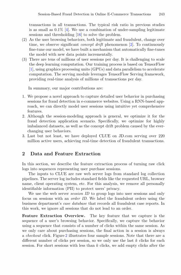
Session-Based Fraud Detection in Online E-Commerce Transactions 243
transactions in all transactions. The typical risk ratio in previous studiesis as small as 0.1% [4]. We use a combination of under-sampling legitimatesessions and thresholding [16] to solve the problem.
(2) As the user browsing behaviors, both legitimate and fraudulent, change overtime, we observe significant concept drift phenomenon [2]. To continuouslyfine-tune our model, we have built a mechanism that automatically fine-tunesthe model with new data points incrementally.
(3) There are tens of millions of user sessions per day. It is challenging to scalethe deep learning computation. Our training process is based on TensorFlow[1], using graphics processing units (GPUs) and data parallelism to acceleratecomputation. The serving module leverages TensorFlow Serving framework,providing real-time analysis of millions of transactions per day.
In summary, our major contributions are:
1. We propose a novel approach to capture detailed user behavior in purchasingsessions for fraud detection in e-commerce websites. Using a RNN-based app-roach, we can directly model user sessions using intuitive yet comprehensivefeatures.
2. Although the session-modeling approach is general, we optimize it for thefraud detection application scenario. Specifically, we optimize for highlyimbalanced datasets, as well as the concept drift problem caused by the ever-changing user behaviors.
3. Last but not least, we have deployed CLUE on JD.com serving over 220million active users, achieving real-time detection of fraudulent transactions.
2 Data and Feature Extraction
In this section, we describe the feature extraction process of turning raw clicklogs into sequences representing user purchase sessions.
The inputs to CLUE are raw web server logs from standard log collectionpipelines. The server log includes standard fields like the requested URL, browsername, client operating system, etc. For this analysis, we remove all personallyidentifiable information (PII) to protect users’ privacy.
We use the web server session ID to group logs into user sessions and onlyfocus on sessions with an order ID. We label the fraudulent orders using thebusiness department’s case database that records all fraudulent case reports. Inthis work, we ignore all sessions that do not lead to an order.
Feature Extraction Overview. The key feature that we capture is thesequence of a user’s browsing behavior. Specifically, we capture the behaviorusing a sequence that consists of a number of clicks within the same session. Aswe only care about purchasing sessions, the final action in a session is alwaysa checkout click. Figure 2 illustrates four sample sessions. Note that there are adifferent number of clicks per session, so we only use the last k clicks for eachsession. For short sessions with less than k clicks, we add empty clicks after the

244 S. Wang et al.
checkout (practically, we pad non-existing sessions with zeros to make the ses-sion sequences the same length). In CLUE, we use a k = 50 that is more thanenough to capture the entire sessions in most of the cases [11].
Fig. 2. Session padding illustration.
Encoding Common Fields of a Click. The standard fields in click logs arestraightforward to encode in a feature vector. For example, we include numericaldata fields like dwell time (i.e. the time a user spends on a particular page) andpage loading time. We encode the fields with categorical types using one-hotencoding. These types include the browser language, text encoding settings,client operating systems, device types and so on. Specifically, for the source IPfield, we first look up the IP address in an IP geo-location database and encodethe location data as categorical data.
Encoding the URL Information. We mainly focus on two URL types:“list.jd.com/∗” and “item.jd.com/∗”, respectively. As there are only dozens ofmerchandise categories, we encode the category using one-hot encoding.
The difficulty is with the items, as there are hundreds of millions of items onJD.com. One-hot encoding will result in a sparse vector with hundreds of millionsof dimensions per click. Even worse, the one-hot encoding eliminates the corre-lations among separate items. Thus, we adopt the Item2Vec [3] to encode items.Item2Vec is a variation of Word2Vec [14], we regard each item as a “word”, whileregarding each session as a “sentence”. So the items that commonly appear atthe same positions of a session are embedded into vectors with smaller Euclideandistance.
We observe that the visit frequency follows a steep power-law distribution.If we choose to cover 90% of all the items in the click history, we only need 25dimensions for Item2Vec, a significant saving on data size. We embed all other10% items that appear rarely as the same constant vector.
In summary, we embed a URL into three parts, the type, category and item.
3 RNN Based Fraudulent Session Detection
Our detection is based on sequences of clicks in a session (as Fig. 2 shows). Wefeed the clicks of the same session into the model in the time order, and we want

Session-Based Fraud Detection in Online E-Commerce Transactions 245
to output a risk score at the last click (i.e. the checkout action) for each session,indicating how suspicious the session is.
To do so, we need a model that can capture a sequence of actions. We findrecurrent neural network (RNN) a good fit. We feed each click to the correspond-ing time slot of the RNN, and the RNN finally outputs the risk score. Figure 3illustrates the RNN structure and its input/output. In the following, we use“depth” and “width” to denote the layer number and the number of hiddenunits per layer, respectively. By default, we use LSTM in CLUE to characterizethe long-term dependency of the prediction on the previous clicks. In Sect. 5, wealso compare the performance of the GRU alternative.
Fig. 3. Illustration of the RNN with LSTM cells.
Dealing with Imbalanced Datasets. One practical problem in fraud detec-tion is the highly imbalanced dataset. In CLUE, we employ both data and modellevel approaches [10].
On the data level, we under-sample the legitimate sessions by random skip-ping, boosting the risk ratio to around 0.5%. After under-sampling, the datasetcontains 1.6 million sessions, among which 8,000 are labeled as fraudulent. Weuse about 6% (about 100,000 sessions) of the dataset as the validation set. Wechoose test sets, with the risk ratio of 0.1%, from the next continuous time period(e.g. two weeks of data), which is outside of the 1.6 million sessions.
On the model level, we leverage the thresholding approach [16] to implementcost-sensitive learning. By choosing the threshold from the range [0, 1], we canobtain an application specific punishment level imposed on the model for mis-classifying minority classes (false negatives) vs. misclassifying the normal class(false positives).
Model Update. To save time, we use incremental data to fine-tune the currentmodel. Our experience shows that the incremental update works both efficientlyand achieves comparable accuracy as the full update. The quality assurancemodule is used to guarantee the performance of the switched model is alwayssuperior to the current model (see Fig. 4).
4 System Architecture and Operation
We have deployed CLUE in real production, analyzing millions of transactionsper day. From an engineering point of view, we have the following design goals:(1) Scalability : CLUE should scale with the growth of the number of transac-tions; (2) Real-time: we need to detect suspicious sessions before the checkout
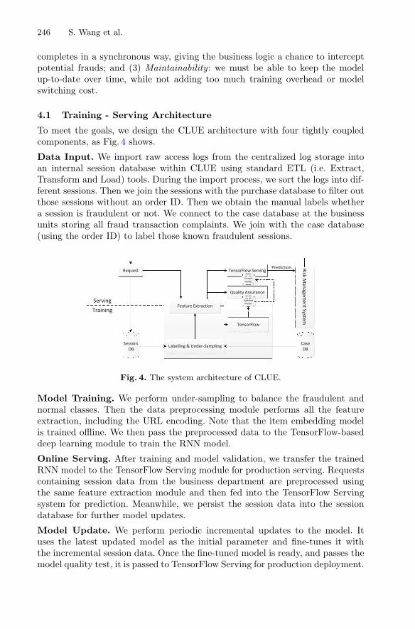
246 S. Wang et al.
completes in a synchronous way, giving the business logic a chance to interceptpotential frauds; and (3) Maintainability : we must be able to keep the modelup-to-date over time, while not adding too much training overhead or modelswitching cost.
4.1 Training - Serving Architecture
To meet the goals, we design the CLUE architecture with four tightly coupledcomponents, as Fig. 4 shows.
Data Input. We import raw access logs from the centralized log storage intoan internal session database within CLUE using standard ETL (i.e. Extract,Transform and Load) tools. During the import process, we sort the logs into dif-ferent sessions. Then we join the sessions with the purchase database to filter outthose sessions without an order ID. Then we obtain the manual labels whethera session is fraudulent or not. We connect to the case database at the businessunits storing all fraud transaction complaints. We join with the case database(using the order ID) to label those known fraudulent sessions.
Fig. 4. The system architecture of CLUE.
Model Training. We perform under-sampling to balance the fraudulent andnormal classes. Then the data preprocessing module performs all the featureextraction, including the URL encoding. Note that the item embedding modelis trained offline. We then pass the preprocessed data to the TensorFlow-baseddeep learning module to train the RNN model.
Online Serving. After training and model validation, we transfer the trainedRNN model to the TensorFlow Serving module for production serving. Requestscontaining session data from the business department are preprocessed usingthe same feature extraction module and then fed into the TensorFlow Servingsystem for prediction. Meanwhile, we persist the session data into the sessiondatabase for further model updates.
Model Update. We perform periodic incremental updates to the model. Ituses the latest updated model as the initial parameter and fine-tunes it withthe incremental session data. Once the fine-tuned model is ready, and passes themodel quality test, it is passed to TensorFlow Serving for production deployment.

Session-Based Fraud Detection in Online E-Commerce Transactions 247
4.2 Implementation Details
For the RNN Training, we set the initial learning rate to 0.001 and let it exponen-tially decay by 0.5 at every 5,000 iterations. We adopt Adam [12] for optimizationwith TensorFlow default configurations. The training process terminates whenthe loss on the validation set stops decreasing. We use TensorFlow as the deeplearning framework [1] and leverage its built-in RNN network. Because of thehighly imbalanced dataset, we raise the batch size to 512. The typical trainingduration is 12 hours (roughly 6–8 epochs).
5 Performance Evaluation
We first present our general detection performance on real production data. Thenwe evaluate the effects of different design choices of CLUE, and their effects onthe model performance, such as different RNN structure, embeddings, and RNNcells. We also compare the RNN-based detection method with other features andlearning methods. Finally, we evaluate the model update results.
5.1 Performance on Real Production Data
The best performance is achieved by an RNN model with 4 layers and 64 unitsper layer with LSTM cells. It is the configuration we use in production. Weevaluate other RNN structures in Sect. 5.2. Compared with traditional machinelearning approaches (see Fig. 5(b)), CLUE achieves over 3x improvement overthe existing system. Integrating CLUE with existing risk management systemsfor eight months in production, we have observed that CLUE has brought asignificant improvement of the system performance.
5.2 Effects of Different RNN Structures
Our model outputs a numerical probability of a session being fraudulent. We usea threshold T to provide a tradeoff between precision and recall [16]. Varying Tbetween [0, 1], we can get the precision of our model corresponding to a particularrecall. Figure 5(a) shows the performance of RNNs with different widths usingthe Precision-Recall (P-R) curve. Throughout the evaluation, we use 4 layers forthe RNN model.
The previous study points out that wider neural networks usually providebetter memorization abilities, while deeper ones are good at generalization [7].We want to evaluate the width and depth of the RNN structure to the frauddetection performance. We use α-β RNN to denote a RNN structure with αlayers and β hidden units per layer.
Table 1 provides the fraud detection precision with 30% recall, using differentα and β. We see that given a fixed width, the performance improves with thedepth increases. However, once the depth becomes too large, overfitting occurs.We find a 4–64 RNN performs the best, outperforming wider models such as
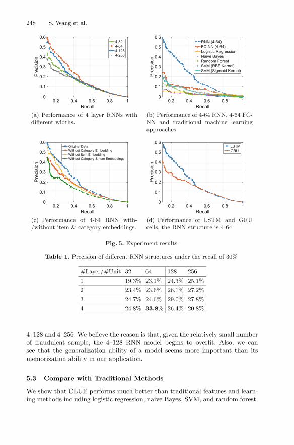
248 S. Wang et al.
Fig. 5. Experiment results.
Table 1. Precision of different RNN structures under the recall of 30%
#Layer/#Unit 32 64 128 256
1 19.3% 23.1% 24.3% 25.1%
2 23.4% 23.6% 26.1% 27.2%
3 24.7% 24.6% 29.0% 27.8%
4 24.8% 33.8% 26.4% 20.8%
4–128 and 4–256. We believe the reason is that, given the relatively small numberof fraudulent sample, the 4–128 RNN model begins to overfit. Also, we cansee that the generalization ability of a model seems more important than itsmemorization ability in our application.
5.3 Compare with Traditional Methods
We show that CLUE performs much better than traditional features and learn-ing methods including logistic regression, naive Bayes, SVM, and random forest.

Session-Based Fraud Detection in Online E-Commerce Transactions 249
Furthermore, we have investigated the performance of fully connected neuralnetworks (FC-NNs). To leverage these methods, we need to leverage traditionalfeature engineering approaches by combining the time-dependent browsing his-tory data into a fixed length vector. We follow many related researches and usebag of words, i.e., count the number of page views of different types of URLs ina session, and summarize the total dwell time of these URLs into the featurevector. Note that with bag-of-word, we cannot leverage the category and itemembedding approaches as introduced in Sect. 2, but we only use one-hot encodingfor these data. We plot the results in Fig. 5(b).
FC-NN performs better than other traditional machine learning methods,indicating that with abundant data, deep learning is not only straightforward toapply but also performs better. Meanwhile, with more detailed feature extrac-tion and time-dependent learning, RNNs perform better than FC-NNs. There-fore, we can infer that our performance improvement comes from two aspects:(1) By using more training data, deep learning (FC-NN) outperforms tradi-tional machine learning approaches; (2) RNN further improves the results overFC-NN as it captures both sequence information, and it allows us to use detailedcategory and item embeddings in the model.
5.4 Effects of Key Design Choices
Here we evaluate the effectiveness of various choices in CLUE’s feature extractionand learning.
Category and Item Embeddings. To show that category and item data areessential features for fraud detection, we remove these features from our clickdata representation. Figure 5(c) shows that the detection accuracy is significantlylower without such information. Clearly, fraudulent users are different from nor-mal users not because they are performing different clicks, but the real differenceis which item they click on and in what order.
Using GRU as RNN Cell. Except for the LSTM, GRU is also an importantRNN cell type that deals with the issues in vanilla RNN. Here we investigate theperformance of RNNs with GRU cells. In Fig. 5(d), we compare the performanceof different RNN cells. We find the LSTM shows better performance.
5.5 Model Update
To show the model update effectiveness using historical data, we consider a fourconsecutive equal-length time periods P1, . . . , P5. The proportion of the numberof sessions contained in these periods is roughly 2:2:1:1:1. We perform two setsof experiments, and both show the effectiveness of our model update methods.
First, we evaluate the performance of using history up to Pn to predict Pn+1.We compare the performance of three update strategies: incremental update, fullupdate (i.e. retrain the model from scratch using all history before the testingperiod) and no update. We use data from P1 to train the initial model. Thenwe compute the precision (setting the recall to 30%) for the following four time
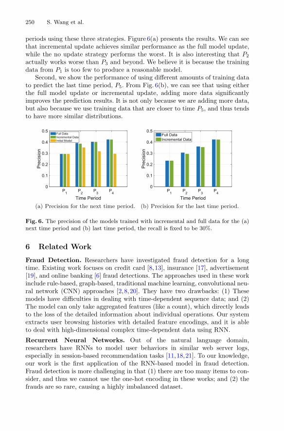
250 S. Wang et al.
periods using these three strategies. Figure 6(a) presents the results. We can seethat incremental update achieves similar performance as the full model update,while the no update strategy performs the worst. It is also interesting that P2
actually works worse than P3 and beyond. We believe it is because the trainingdata from P1 is too few to produce a reasonable model.
Second, we show the performance of using different amounts of training datato predict the last time period, P5. From Fig. 6(b), we can see that using eitherthe full model update or incremental update, adding more data significantlyimproves the prediction results. It is not only because we are adding more data,but also because we use training data that are closer to time P5, and thus tendsto have more similar distributions.
Fig. 6. The precision of the models trained with incremental and full data for the (a)next time period and (b) last time period, the recall is fixed to be 30%.
6 Related Work
Fraud Detection. Researchers have investigated fraud detection for a longtime. Existing work focuses on credit card [8,13], insurance [17], advertisement[19], and online banking [6] fraud detections. The approaches used in these workinclude rule-based, graph-based, traditional machine learning, convolutional neu-ral network (CNN) approaches [2,8,20]. They have two drawbacks: (1) Thesemodels have difficulties in dealing with time-dependent sequence data; and (2)The model can only take aggregated features (like a count), which directly leadsto the loss of the detailed information about individual operations. Our systemextracts user browsing histories with detailed feature encodings, and it is ableto deal with high-dimensional complex time-dependent data using RNN.
Recurrent Neural Networks. Out of the natural language domain,researchers have RNNs to model user behaviors in similar web server logs,especially in session-based recommendation tasks [11,18,21]. To our knowledge,our work is the first application of the RNN-based model in fraud detection.Fraud detection is more challenging in that (1) there are too many items to con-sider, and thus we cannot use the one-hot encoding in these works; and (2) thefrauds are so rare, causing a highly imbalanced dataset.
Session-Based Fraud Detection in Online E-Commerce Transactions 251
7 Conclusion and Future Work
Frauds are intrinsically difficult to analyze, as they are engineered to avoid detec-tion. Luckily, we are able to observe millions of transactions per day, and thusaccumulate enough fraud samples to train an extremely detailed RNN model thatcaptures not only the detailed click information but also the exact sequences.With proper handling of imbalanced learning, concept drift, and real-time serv-ing problems, we show that our features and model, seemingly detailed andexpensive to compute, actually scale to support the transaction volumes wehave, while providing an accuracy never achieved by traditional methods basedon aggregate features. Moreover, our approach is straightforward, without toomuch ad hoc feature engineering, showing another benefit of using RNN.
As future work, we can further improve the performance of CLUE by build-ing a richer history of a user, including non-purchasing sessions. We are alsogoing to apply the RNN-based representation of sessions into other tasks likerecommendation or merchandising.
Acknowledgement. We would like to thank our colleagues at JD for their help dur-ing this research. This research is supported in part by the National Natural ScienceFoundation of China (NSFC) grant 61532001, Tsinghua Initiative Research ProgramGrant 20151080475, MOE Online Education Research Center (Quantong Fund) grant2017ZD203, and gift funds from Huawei.
References
1. Abadi, M., Agarwal, A., Barham, P., Brevdo, E., Chen, Z., Citro, C., Corrado, G.S.,Davis, A., Dean, J., Devin, M., et al.: TensorFlow: large-scale machine learning onheterogeneous distributed systems. arXiv:1603.04467 (2016)
2. Abdallah, A., Maarof, M.A., Zainal, A.: Fraud detection system: a survey. J. Netw.Comput. Appl. 68, 90–113 (2016)
3. Barkan, O., Koenigstein, N.: Item2Vec: neural item embedding for collaborativefiltering. In: IEEE 26th International Workshop on Machine Learning for SignalProcessing, pp. 1–6. IEEE (2016)
4. Bellinger, C., Drummond, C., Japkowicz, N.: Beyond the boundaries of SMOTE.In: Frasconi, P., Landwehr, N., Manco, G., Vreeken, J. (eds.) ECML PKDD 2016.LNCS (LNAI), vol. 9851, pp. 248–263. Springer, Cham (2016). https://doi.org/10.1007/978-3-319-46128-1 16
5. Bianchi, C., Andrews, L.: Risk, trust, and consumer online purchasing behaviour:a chilean perspective. Int. Mark. Rev. 29(3), 253–275 (2012)
6. Carminati, M., Caron, R., Maggi, F., Zanero, S., Epifani, I.: BankSealer: a decisionsupport system for online banking fraud analysis and investigation. Comput. Secur.53, 175–186 (2015)
7. Cheng, H.T., Koc, L., Harmsen, J., Shaked, T., Chandra, T., Aradhye, H.,Anderson, G., Corrado, G., Chai, W., Ispir, M., et al.: Wide & deep learningfor recommender systems. In: Proceedings of the 1st Workshop on Deep Learningfor Recommender Systems, pp. 7–10. ACM (2016)

252 S. Wang et al.
8. Fu, K., Cheng, D., Tu, Y., Zhang, L.: Credit card fraud detection using convo-lutional neural networks. In: Hirose, A., Ozawa, S., Doya, K., Ikeda, K., Lee, M.,Liu, D. (eds.) ICONIP 2016. LNCS, vol. 9949, pp. 483–490. Springer, Cham (2016).https://doi.org/10.1007/978-3-319-46675-0 53
9. Glover, S., Benbasat, I.: A comprehensive model of perceived risk of e-commercetransactions. Int. J. Electron. Commer. 15(2), 47–78 (2010)
10. He, H., Garcia, E.A.: Learning from imbalanced data. IEEE Trans. Knowl. DataEng. 21(9), 1263–1284 (2009)
11. Hidasi, B., Quadrana, M., Karatzoglou, A., Tikk, D.: Parallel recurrent neural net-work architectures for feature-rich session-based recommendations. In: Proceedingsof the 10th ACM Conference on Recommender Systems, pp. 241–248 (2016)
12. Kingma, D.P., Ba, J.: Adam: A method for stochastic optimization.arXiv:1412.6980 (2014)
13. Lim, W.Y., Sachan, A., Thing, V.: Conditional weighted transaction aggregationfor credit card fraud detection. Adv. Inf. Commun. Technol. 433, 3–16 (2014)
14. Mikolov, T., Sutskever, I., Chen, K., Corrado, G.S., Dean, J.: Distributed repre-sentations of words and phrases and their compositionality. In: Advances in NeuralInformation Processing Systems, pp. 3111–3119 (2013)
15. Phua, C., Alahakoon, D., Lee, V.: Minority report in fraud detection: classificationof skewed data. ACM SIGKDD Explor. Newslett. 6(1), 50–59 (2004)
16. Sheng, V.S., Ling, C.X.: Thresholding for making classifiers cost-sensitive. In:National Conference on Artificial Intelligence, pp. 476–481 (2006)
17. Shi, Y., Sun, C., Li, Q., Cui, L., Yu, H., Miao, C.: A fraud resilient medical insur-ance claim system. In: Thirtieth AAAI Conference, pp. 4393–4394 (2016)
18. Tan, Y.K., Xu, X., Liu, Y.: Improved recurrent neural networks for session-basedrecommendations. In: Proceedings of the 1st Workshop on Deep Learning for Rec-ommender Systems, pp. 17–22. ACM (2016)
19. Tian, T., Zhu, J., Xia, F., Zhuang, X., Zhang, T.: Crowd fraud detection in inter-net advertising. In: International Conference on World Wide Web, pp. 1100–1110(2015)
20. Tseng, V.S., Ying, J.C., Huang, C.W., Kao, Y., Chen, K.T.: FrauDetector: a graph-mining-based framework for fraudulent phone call detection. In: ACM SIGKDDInternational Conference on Knowledge Discovery and Data Mining, pp. 2157–2166(2015)
21. Wu, S., Ren, W., Yu, C., Chen, G., Zhang, D., Zhu, J.: Personal recommendationusing deep recurrent neural networks in NetEase. In: International Conference onData Engineering, pp. 1218–1229 (2016)
SINAS: Suspect Investigation Using Offenders’Activity Space
Mohammad A. Tayebi1(B), Uwe Glasser1, Patricia L. Brantingham2,and Hamed Yaghoubi Shahir1
1 School of Computing Science, Simon Fraser University, Burnaby, Canada{tayebi,glaesser,syaghoub}@cs.sfu.ca
2 School of Criminology, Simon Fraser University, Burnaby, [email protected]
Abstract. Suspect investigation as a critical function of policing deter-mines the truth about how a crime occurred, as far as it can befound. Understanding of the environmental elements in the causes ofa crime incidence inevitably improves the suspect investigation process.Crime pattern theory concludes that offenders, rather than venture intounknown territories, frequently commit opportunistic and serial violentcrimes by taking advantage of opportunities they encounter in placesthey are most familiar with as part of their activity space. In this paper,we present a suspect investigation method, called SINAS, which learnsthe activity space of offenders using an extended version of the randomwalk method based on crime pattern theory, and then recommends thetop-K potential suspects for a committed crime. Our experiments on alarge real-world crime dataset show that SINAS outperforms the baselinesuspect investigation methods we used for the experimental evaluation.
1 Introduction
Crime is a purposive deviant behavior that is an integrated result of differentsocial, economical and environmental factors. Crime imposes substantial costson society at individual, community, and national levels.
An important policing task is investigating committed or reported crimes—known as criminal or suspect investigation. Spatial studies of crime, and morespecifically environmental criminology, play an essential role in criminal intelli-gence [1,5–8].
Modeling spatial aspects of criminal behavior can be seen as an intractablecase of the human mobility problem [2,4]. This is mainly because available infor-mation about the spatial life of offenders is usually limited to police arrest dataon their home and crime locations. Further, spatial displacement of crime is acommon phenomenon, meaning offenders shift their crime locations.
In this paper, we propose an approach to Suspect INvestigation using offend-ers’ Activity Space, called SINAS. It first learns activity space of offenders basedon crime pattern theory, using existing crime records. Then, given the location
c© Springer International Publishing AG 2017Y. Altun et al. (Eds.): ECML PKDD 2017, Part III, LNAI 10536, pp. 253–265, 2017.https://doi.org/10.1007/978-3-319-71273-4_21
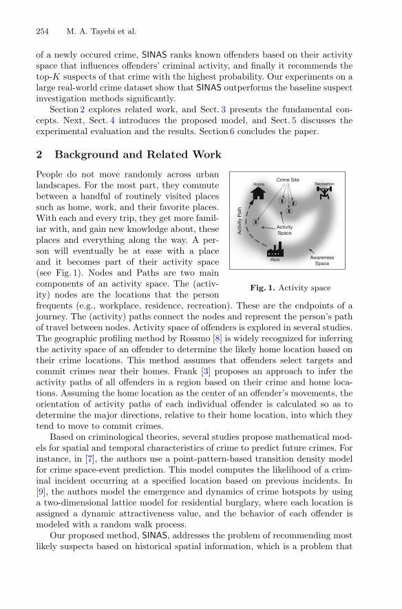
254 M. A. Tayebi et al.
of a newly occured crime, SINAS ranks known offenders based on their activityspace that influences offenders’ criminal activity, and finally it recommends thetop-K suspects of that crime with the highest probability. Our experiments on alarge real-world crime dataset show that SINAS outperforms the baseline suspectinvestigation methods significantly.
Section 2 explores related work, and Sect. 3 presents the fundamental con-cepts. Next, Sect. 4 introduces the proposed model, and Sect. 5 discusses theexperimental evaluation and the results. Section 6 concludes the paper.
2 Background and Related Work
Fig. 1. Activity space
People do not move randomly across urbanlandscapes. For the most part, they commutebetween a handful of routinely visited placessuch as home, work, and their favorite places.With each and every trip, they get more famil-iar with, and gain new knowledge about, theseplaces and everything along the way. A per-son will eventually be at ease with a placeand it becomes part of their activity space(see Fig. 1). Nodes and Paths are two maincomponents of an activity space. The (activ-ity) nodes are the locations that the personfrequents (e.g., workplace, residence, recreation). These are the endpoints of ajourney. The (activity) paths connect the nodes and represent the person’s pathof travel between nodes. Activity space of offenders is explored in several studies.The geographic profiling method by Rossmo [8] is widely recognized for inferringthe activity space of an offender to determine the likely home location based ontheir crime locations. This method assumes that offenders select targets andcommit crimes near their homes. Frank [3] proposes an approach to infer theactivity paths of all offenders in a region based on their crime and home loca-tions. Assuming the home location as the center of an offender’s movements, theorientation of activity paths of each individual offender is calculated so as todetermine the major directions, relative to their home location, into which theytend to move to commit crimes.
Based on criminological theories, several studies propose mathematical mod-els for spatial and temporal characteristics of crime to predict future crimes. Forinstance, in [7], the authors use a point-pattern-based transition density modelfor crime space-event prediction. This model computes the likelihood of a crim-inal incident occurring at a specified location based on previous incidents. In[9], the authors model the emergence and dynamics of crime hotspots by usinga two-dimensional lattice model for residential burglary, where each location isassigned a dynamic attractiveness value, and the behavior of each offender ismodeled with a random walk process.
Our proposed method, SINAS, addresses the problem of recommending mostlikely suspects based on historical spatial information, which is a problem that

SINAS: Suspect Investigation Using Offenders’ Activity Space 255
none of the existing methods is able to address. Thus, there is a challenge inevaluating our experimental results. The model in [7] predicts only the time andlocation of crimes at an aggregate level. The method proposed in [8] discoversoffender home locations based on their crime locations. Finally, the method in [3]finds locations which are centers of interest for committing crime.
3 Crime Data Characteristics
We evaluate the efficacy of our approach on a crime dataset representing fiveyears (2001–2006) of police arrest-data for the Province of British Columbia,comprising several million data records, each refers to a reported offence1. Ourexperiments consider all subjects in four main categories: charged, chargeable,charge recommended, and suspect. Being in one of these categories means that thepolice is serious enough about the subject’s involvement in a crime as to warrantcalling them ‘offender’. Here, we concentrate on crimes in Metro Vancouver(population: 2.46 M), with different regions connected through a road networkcomposed of road segments having an average length of 0.2 km (see Table 1).
Table 1. Statistical properties of the used dataset
Property Value Property Value
#crimes 125,927 #offenders 189,675
#offenders with more then 1 crime 25,162 #co-offending links 68,577
#co-offenders in co-offending network 17,181 Avg. node degree in co-offending network 4
#road-segments 64,108 Avg. crime per road segment 2
Figures 2a and b illustrate the distribution function of crime incidents peroffender and per road segment respectively. Both distributions have heavy-tailedpattern. 83% of the offenders committed only one crime, while less than 1% ofthe offenders committed 10 or more crimes. Further, 38% of the road segmentsare linked to at least one crime and 9% of the road segments are linked to 10 ormore crimes. Half of all the crimes occurred in only 1% of all road segments, anda total of 25% of all the crimes occurred in only 100 road segments. The averagehome to crime location distance of 80%, 63% and 40% of all offenders is less than10 km, 5 km and 2 km, respectively. The average crime location distance of 73%,52% and 26% of all offenders is less than 10 km, 5 km and 2 km, respectively.One can assume that frequent offenders are generally mobile and have severalhome locations identified in their records. 41% of the offenders who committedmore than one crime have more than one home location.
1 This data was made available for research purpose by Royal Canadian MountedPolice (RCMP) and retrieved from the Police Information Retrieval System (PIRS).

256 M. A. Tayebi et al.
Fig. 2. Distribution of: (a) crimes per offender; (b) crimes per road segment
3.1 Fundamental Concepts and Definitions
This section introduces the fundamental concepts, definitions, and notations.
Offender. Let V be a set of offenders and C be a set of crimes. Each crimeevent e ∈ C involves a non-empty subset of criminal offenders U ⊆ V . Ci is theset of crimes committed by offender ui. With each crime incident we associate atype of crime, a time when the crime occurred as well as longitude and latitudecoordinates of the crime location and home location of involved offenders.
Co-offending Network. A co-offending network is an undirected graphG(V,E). Each node represents a known offender ui ∈ V . Offenders u and vare connected, ui, uk ∈ V and (ui, uk) ∈ E, if they are known to have commit-ted one or more offences together, and are not connected otherwise. Γi denotesthe set of neighbors of offender ui in the co-offending network.
Road Network. Intuitively, a road network can be decomposed into road seg-ments, each of which starts and ends at an intersection. We use the dual rep-resentation where the role of roads and intersections is reversed. All physicallocations along the same road segment are mapped to the same node. Formally,a road network is an undirected graph R(L,Q), where L is a set of nodes, eachrepresenting a single road segment. Road segments lj and lk are connected,{lj , lk} ∈ Q, if they have an adjacent intersection in common. Crime locationswithin a studied geographic boundary are mapped to the closest road segment.Henceforth, the term “road” is used to refer to a road segment.
Road Features. A vector yj denotes the features of the road lj including roadlength dj , and road attractiveness features vector aj . Further, aj is a vector ofsize m where the value of the kth entry of aj corresponds to the total numberof crimes of type k committed previously at lj . Πj denotes the set of neighborsof road lj in the road network. Δ ⊂ L denotes a set of roads with the highestcrime rate, called crime hotspots. Dlj ,lk is the shortest path distance of road ljfrom road lk, and fj denotes the total number of crimes at road lj .
Anchor Locations. Li is the set of roads at which offender ui has beenobserved, including all of his known home and crime locations. fi,j and ti,j

SINAS: Suspect Investigation Using Offenders’ Activity Space 257
respectively denote the frequency and the last time ui was at anchor location lj .Offender trend is given by a vector xi of size m which indicates the crime trendof ui as extracted from his criminal history. That is, the value of the kth entryof xi corresponds to the number of crimes of type k committed by offender ui.
3.2 Problem Scope
Crime analysis captures a broad spectrum of facets pertaining to different needsand using different analytical methods. For instance, intelligence analysis aimsat recognizing relationships between criminal network actors to identify andarrest offenders. It typically starts with a known crime problem or identifiedco-offending network, then uses these resources to collect, analyze and compileinformation about a predetermined target. An important problem is to identifymost likely perpetrators of previous crimes. Criminal profiling approaches con-tribute to criminal intelligence using offenders’ characteristics. Also, methodslike geographic profiling build on environmental criminology theories and useinformation related to the environment of offenders and crimes.
Problem Definition—Suspect Investigation: In the following, we formallyaddress the problem of suspect investigation. Assume there is a collection ofcrime records, C, from past crime events where each element in C uniquelyidentifies a single crime incident. When a new crime incident e occurs, policeinvestigates suspects who potentially committed e based on the existing infor-mation, that is, anchor locations (home and crime locations) of every offenderin C mapped on a road network, the type of crimes they committed, and alsothe (known) co-offending network G extracted from C. The problem definitionin abstract formal terms is as follows:
Given a crime dataset C and new crime incident e at location le, the goalis to recommend the top-K suspects for e with the highest probability.
Geographic profiling addresses a similar problem of detecting home locations ofsuspects of a crime incident, given a series of past crimes. However, the noveltyof our approach is two-fold: (1) it directly targets the identity of offenders ratherthan their home locations; and (2) the input of our approach is a single crimeincident, while the input of geographic profiling is a series of crimes.
4 SINAS Method
4.1 Learning Activity Space
A random walk over a graph is a stochastic process in which the initial state isknown and the next state is decided using a transition probability matrix thatidentifies the probability of moving from a node to another node of the graph.Under certain conditions, the random walk process converges to a stationarydistribution assigning an importance value to each node of the graph. The ran-dom walk method can be modified to satisfy the locality aspect of crimes, which

258 M. A. Tayebi et al.
states that offenders do not attempt to move far from their anchor locations.For instance, the random walk method works locally if the likelihood of termi-nating the walk increases with the distance from the anchor locations.
In our proposed model, starting from an anchor location the offender exploresthe city through the underlying road network. At each road, he decides whetherto proceed to a neighboring road or return to one of his anchor locations. Therandom walk process continues until it converges to a steady state which reflectsthe probability of visiting a road by the offender. This probability can be relevantto the offender’s exposure to a crime opportunity.
For learning the activity space of an offender, we need to understand his dailylife and routines. However, in the crime dataset, generally we miss the pathscompletely and the nodes partially. Thus, we improve our incomplete knowledgeabout offenders with available information in the dataset by defining two dif-ferent sets of anchor locations: (1) main anchor locations, denoted by Li foroffender ui, is an extension of the offender anchor locations by adding his co-offenders’ anchor locations with the assumption that friends in the co-offendingnetwork are likely to share the same locations; and (2) intermediate anchor loca-tions, denoted by Ii for offender ui, is the roads closest to the set of his mainanchor locations, using a Gaussian model (see Sect. 4.1–Starting Probabilitiesfor details).
An offender starts his random walk either from a main or intermediate anchorlocation. Given that the actual trajectories in an offender’s journey to crime areunknown, SINAS guides offender movements in directions with a higher chanceof committing a crime. This is done by taking into account different aspectsthat influence the offender movement directionality in computing the transitionprobabilities in a random walk.
Random Walk Process: For each single offender ui, we perform a series ofrandom walks on the road network R(L,Q). The random walk process startsfrom one of the anchor locations of ui with predefined probabilities (see Sect. 4.1–Starting Probabilities) and traverses the road network to locate a criminal oppor-tunity. At each step k of the random walk, the offender is at a certain road lj andmakes one of two possible decisions: (1) With probability α, he decides to returnto an anchor location and not look for a criminal opportunity this time, choosingan anchor location as follows: (a) with probability β, he decides to return to amain anchor location l ∈ Li, and (b) with probability 1 − β, he returns to anintermediate anchor location l ∈ Ii; and (2) With probability 1−α he continueslooking for a crime opportunity. If he continues his random walk then he hastwo options in each step of the walk: (a) with probability θ(ui, lj , k), he stopsthe random walk, which means the offender commits a crime at road lj , and(b) with probability 1 − θ(ui, lj , k) he continues the random walk, moving toanother road which is a direct neighbor of lj .
To continue the random walk at road lj , we select a direct neighbor roadfrom Πlj . Function φ computes the transition probability from a roadsegment

SINAS: Suspect Investigation Using Offenders’ Activity Space 259
to one of its neighbor road segments (see Sect. 4.1–Movement Directionality fordetails). The probability of selecting road segment lr in the next step is:
P (lj → lr) =φ(lr)∑
lp∈πlj
φ(lp)(1)
The probability of being at road lr at step k+1 given that the offender was atroad lj at step k is shown in Eq. 2, where Xui,k is the random variable for ui beingat road lr in step k. We terminate the random walks when ||Fm+1||−||Fm|| ≤ ε,where Fm = (F (ui, l1) . . . F (ui, l|L|))T is the results for ui after m random walks.For some offenders the random walks do not converge, in which case we terminatethe overall process at m > 10000.
P (Xui,k+1 = lr|Xui,k = lj) = (1 − α)(1 − θlj ,k) × P (lj → lr) (2)
Starting Probabilities: The model distinguishes two types of starting nodes.(1) Main anchor locations are all anchor locations of a single offender and hisco-offenders: Li = Li ∪ {lj : lj ∈ Lv, v ∈ Γu}. The rationale is that offenderswho have collaborated in the past likely may have shared information on anchorlocations in their activity space, an aspect that possibly affects their choice offuture crime locations. In computing the starting probability of each anchorlocation, the two primary factors are the frequency and the last time an offendervisited an anchor location. The probability that offender ui starts his randomwalk from lj is shown in Eq. 3, where t is the current time, and ρ is the parametercontrolling the effect of the timing.
S(i, j) =fi,j × e
−(t−ti,j)ρ
∑
lk∈Li
fi,k × e−(t−ti,k)
ρ
(3)
(2) Intermediate anchor locations are the closest locations to main anchor loca-tions. Human mobility models use Gaussian distributions to analyze humanmovement around a particular point such as home or work location [4]. Weassume that offender movement around their main anchor locations follows aGaussian distribution. Each main anchor location of offender ui is used as thecenter, and the probability of ui being located in a road is modeled with aGaussian distribution. Given road l, the probability of ui residing at l is:
S(i, l) =∑
lj∈Li
fi,j∑
lk∈Li
fi,k
N (l|μlj , Σlj )∑
lk∈Li
N (l|μlk , Σlk)(4)
Here l is a road which does not belong to the set of main anchor locations.N (l|μlj , Σlj ) is a Gaussian distribution for visiting a road when ui is at anchorlocation lj , with μlj and Σlj as mean and covariance. We consider the normalizedactivity frequency of ui at lj , meaning that a main anchor location with higher

260 M. A. Tayebi et al.
activity frequency has higher importance. For offender ui, the roads with thehighest probability of being an intermediate anchor location are added to theset Ii as additional starting nodes besides the main anchor locations.
Movement Directionality: The creation of the main attractor nodes andpaths are developed through normal mobility shaped by the urban backclothor urban environment. Each individual has normal, routine pathways or com-muting/mobility routes that are unique. However, the environment where welive influences our actions and movements. Highways, streets and road networksin general guide us to our destinations such as home, workplace, recreation cen-ter, and business establishments. In the aggregate, individuals routes overlap orintersect in time and space. These areas of overlap often have rush hours andcongestion at intersections or mass transit stops associated with handling largenumbers of people. These high activity locations can become crime attractorsand crime generators when there are enough suitable targets in those locations.Crime attractors and generators affect directionality of offenders’ movement.
One can conclude that starting from an anchor location the probability ofoffender movement toward crime attractors and generators is higher. To addressthis fact, in the random walk process, the transition probability is computedbased on the proximity of a road to the crime hotspots and the importanceof each crime hotspot, which is proportional to the number of crimes commit-ted there. Function φ(lj) is used in computing the transition probability (seeSect. 4.1–Random Walk Process) of moving offender ui from lk to lj , where fn
is the number of crimes committed at ln. Dj,n is the distance of road lj fromthe hotspot ln ∈ Δ, which is equal to the length of shortest path between tworoads.
φ(lj) =|Δ|∑
n=1
fn × 1Dj,n
(5)
Stopping Criteria: The probability of stopping the random walk for an offenderat a given road corresponds to the probability of this offender committing a crimein that road segment. Two factors influence the stopping probability of offenderui in the road lj . The first one relates to the similarity of the crime trend ofoffender ui and the criminal attractiveness of road lj , where higher similaritymeans a higher chance of stopping ui at lj . The second factor is the distance oflj from the starting point measured in the number of steps (k) from the startingpoint. To satisfy the locality aspect of crimes, the probability of continuing therandom walk decrease while getting farther from the starting point. Thus, thestopping probability (Eq. 6) is inversely proportional to k. Also, sim(i, j) denotesthe cosine similarity of crime trend of ui and the attractiveness of lj .
θ(ui, lj , k) = sim(i, j) × 1
1 + e−k2
(6)
4.2 Suspect Recommendation
The crime location is neither even nor random, however, there is an underlyingspatial pattern in it. Environmental criminology theories [1] suggest that crimes

SINAS: Suspect Investigation Using Offenders’ Activity Space 261
occur in predictable ways, at offenders’ awareness space which includes theiractivity space. To recommend the most likely suspects of a new crime incidentbased on the learnt offenders’ activity space, we rank offenders based on theproximity of the crime location to their activity spaces. An offender is consideredas a ‘potential suspect’ if the crime location is close enough to the activity spaceof this offender. This approach is based on a crime pattern theory stating thatfuture crime locations are within offenders’ activity space which is dependent totheir activity nodes and paths. To influence offenders’ characteristics, we considerthe history of the offenders including the types and number of their committedcrimes. The probability of offender ui commits a new crime e is computed inEq. 7, where T (Ci, e) is a boolean function that returns one if in the crimerecords of offender ui, Ci, there is a crime event with the same type as crime e,and zero otherwise. ω is a parameter that controls the influence of function T .|Ci| is the number of crimes that offender ui committed previously. F (ui, lk) isthe probability of lk being in activity space of offender ui. Dlk,le is the distancebetween roads lk and le.
Z(ui, e) = ωT (Ci, e) × |Ci| ×n∑
k=1
F (ui, lk) × Dlk,le (7)
5 Experimental Evaluation
We divide the crime dataset chronologically into train and test data. The traindata, used to learn the activity space of offenders, includes all crimes that hap-pened in the first 54 months, and the test data includes the remaining six months.The crimes in the test data committed by known offenders are used for suspectinvestigation. SINAS recommends the top-K suspects most likely to commit anew occurred crime. K is set to 50 in our experiments, but relative results forother values of K are also consistent. We use the recall measure (i.e., the per-centage of crimes in which the offender who committed that crime appears inthe list of top-K recommended suspects) to evaluate the quality of methods.Before discussing the results, it is crucial to specify the experimental setting.
(1) On the one hand, if a new crime occurs in a location where an offenderhas been observed previously (as his anchor location) then the probability thatthe same offender is involved in the new crime is higher, and this fact makesthe investigation process easier. Formally speaking: assume a crime e committedby offender ui at lj . If lj ∈ Li, then we consider e as an easy case; and, iflj /∈ Li, then we consider e as a hard case. We therefore define two scenarios:easy scenario which includes all (union of easy and hard) cases and hard scenariowhich only includes hard cases. We compare the performance of SINAS for botheasy and hard scenarios.
(2) On the other hand, repeat offenders are responsible for large percentageof committed crimes and there has long been an interest in the behavior of repeatoffenders since controlling these groups of offenders can significantly reduce theoverall crime level. Therefore, we distinguish two groups of offenders: repeat

262 M. A. Tayebi et al.
offenders with 10 or more crimes and non-repeat offenders with less than 10crimes. We compare the performance of SINAS for repeat offenders with all(union of repeat and non-repeat) offenders.
5.1 Baseline Methods
As discussed in Sect. 2, there is no suspect investigation method using offend-ers’ spatial information to the best of our knowledge; however, we evaluate theSINAS performance in comparison with some baseline methods. We also per-form experiments on different settings of SINAS to learn the meaningfulness ofits three principal elements: (1) the probabilistic aspect of offenders’ activityspace, (2) offenders’ crime types, and (3) the frequency of crimes committed byoffenders. Following is the list of comparison partners in our experiments.
SINAS-PPN takes the probabilistic aspect of offenders’ activity space andtheir crime types into account while ignoring the frequency of committed crimes.
SINAS-PNP takes the probabilistic aspect of offenders’ activity space andfrequency of committed crimes into account while ignoring the type of crimes.
SINAS-NPP ignores the probabilistic aspect of offenders’ activity space butconsiders type and frequency of crimes committed by them.
SINAS takes all available information including the probabilistic aspect ofoffenders’ activity space, frequency and type of committed crimes into account.
CrimeFrequency ranks offenders based on the number of crimes they havecommitted and includes top-K offenders with the highest crime number in therecommendation list. The intuition behind this method is that repeat offendersare more probable to be involved in a new occurred crime.
Proximity uses a distance-decay function to compute the proximity ofoffenders’ anchor locations from the location of a new crime. It considers thefrequency of being an offender in each of his anchor locations as a factor of theirimportance. Proximity is comparable to the geographic profiling approach [8].
Random recommends suspects randomly from the pool of known offenders.
5.2 Experimental Results
Table 2 shows the performance of different variations of SINAS and the otherbaseline methods for both easy and hard scenarios. For both scenarios, SINASoutperforms the other baseline methods and significantly outperforms Proximityand CrimeFrequency. Interestingly, CrimeFrequency has a good performance inthe easy scenario. In the easy scenario that crimes with known locations for
Table 2. Recall (%) of different suspect investigation methods (K = 50) for hard andeasy scenarios considering all offenders (repeat and non-repeat)
SINAS-PPN SINAS-PNP SINAS-NPP SINAS CrimeFrequency Proximity Random
Hard scenario 3.8 5.1 4.2 5.4 1.5 3.7 0.002
Easy scenario 10.4 11.9 5.3 12.1 1.3 10.3 0.002
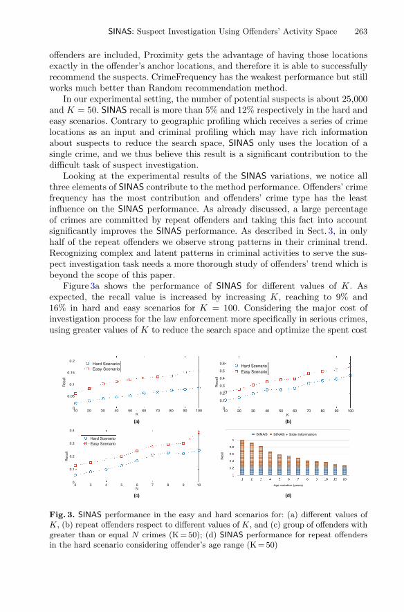
SINAS: Suspect Investigation Using Offenders’ Activity Space 263
offenders are included, Proximity gets the advantage of having those locationsexactly in the offender’s anchor locations, and therefore it is able to successfullyrecommend the suspects. CrimeFrequency has the weakest performance but stillworks much better than Random recommendation method.
In our experimental setting, the number of potential suspects is about 25,000and K = 50. SINAS recall is more than 5% and 12% respectively in the hard andeasy scenarios. Contrary to geographic profiling which receives a series of crimelocations as an input and criminal profiling which may have rich informationabout suspects to reduce the search space, SINAS only uses the location of asingle crime, and we thus believe this result is a significant contribution to thedifficult task of suspect investigation.
Looking at the experimental results of the SINAS variations, we notice allthree elements of SINAS contribute to the method performance. Offenders’ crimefrequency has the most contribution and offenders’ crime type has the leastinfluence on the SINAS performance. As already discussed, a large percentageof crimes are committed by repeat offenders and taking this fact into accountsignificantly improves the SINAS performance. As described in Sect. 3, in onlyhalf of the repeat offenders we observe strong patterns in their criminal trend.Recognizing complex and latent patterns in criminal activities to serve the sus-pect investigation task needs a more thorough study of offenders’ trend which isbeyond the scope of this paper.
Figure 3a shows the performance of SINAS for different values of K. Asexpected, the recall value is increased by increasing K, reaching to 9% and16% in hard and easy scenarios for K = 100. Considering the major cost ofinvestigation process for the law enforcement more specifically in serious crimes,using greater values of K to reduce the search space and optimize the spent cost
Fig. 3. SINAS performance in the easy and hard scenarios for: (a) different values ofK, (b) repeat offenders respect to different values of K, and (c) group of offenders withgreater than or equal N crimes (K = 50); (d) SINAS performance for repeat offendersin the hard scenario considering offender’s age range (K = 50)
264 M. A. Tayebi et al.
and time is reasonable. Figure 3b shows the performance of SINAS for the repeatoffenders with respect to different values of K. For K = 50, SINAS has the recallof 25% and 38% in the hard and easy scenarios. For the repeat offenders that weknow more about their spatial activities, the SINAS performance is about twotimes greater than the method performance for all offenders.
For studying the SINAS performance for repeat and not-repeat offenders,we categorize offenders based on the number of crimes they have committed.Figure 3c shows the SINAS recall for each of these groups of offenders. Asdepicted, the SINAS performance increases linearly by increasing the numberof crimes of the corresponding group, meaning that suspect investigation for agroup of offenders who committed more crimes is generally more successful.
SINAS and criminal profiling approaches can be used as complementary toolsfor suspect investigation. Assume that for a new occurred crime, the police is ableto guess the age of the offender based on evidence and witness interviews. Usingthis piece of information reduces the search space and increases the chance ofsuccess. In the following, we discuss the experimental results of applying SINASon this subset of offenders instead of all offenders. Figure 3d shows the result forthis suspect intelligence scenario (K = 50), where the x-axis shows the exactnessof our knowledge about the age (#years) of the offender. In other words, ifthe offender exact age is a, then the value b on x-axis means SINAS considersoffenders with ages in the interval of [a−b, a+b]. As shown, having more preciseinformation on the offender’s age contributes more to the intelligence process.
With b = 1, SINAS is able to investigate all crimes successfully, and evenb = 20 improves the SINAS performance compared to the situation of havingno side information. This result shows the importance of side information in thesuspect investigation process.
6 Conclusions
This paper proposes the SINAS method for suspect investigation by analyz-ing the activity space of offenders. It utilizes an extended version of the ran-dom walk method and learns the activity space of offenders based on a widelyaccepted criminological theory, crime pattern theory. Our experimental resultsshow: (1) learning the activity space of offenders from their spatial life con-tributes to high-quality suspect recommendation; (2) utilizing offenders’ crimi-nal trend improves suspect recommendation. Not only does SINAS significantlyoutperform baseline methods for both repeat and non-repeat offenders, but italso has more satisfying results for repeat offenders where there is more infor-mation available on their spatial activities; and (3) SINAS and criminal profilingapproaches can be viewed as complementary tools for suspect investigation.
Data mining-based suspect investigation is a multi-step process that has sig-nificant operational challenges in practice. Three main steps of this process—question formulation, data preparation, and data mining—have been addressedin our proposed method. However, the ultimate steps, deployment and efficacyevaluation, are beyond the scope of this paper. Making a difference in real-world

SINAS: Suspect Investigation Using Offenders’ Activity Space 265
situations, calls for an iterative process where law enforcement and policymakersact on analytics inferred from data mining-based suspect investigation methodsat the strategic, tactical and operational levels.
References
1. Brantingham, P.J., Brantingham, P.L.: Environmental Criminology. Sage Publica-tions, Beverly Hills (1981)
2. Brockmann, D., Hufnagel, L., Geisel, T.: The scaling laws of human travel. Nature439(7075), 462–465 (2006)
3. Frank, R., Kinney, B.: How many ways do offenders travel - evaluating the activitypaths of offenders. In: Proceedings of the 2012 European Intelligence and SecurityInformatics Conference (EISIC 2012), pp. 99–106 (2012)
4. Gonzalez, M.C., Hidalgo, C.A., Barabasi, A.: Understanding individual humanmobility patterns. Nature 453(7196), 779–782 (2008)
5. Gorr, W., Harries, R.: Introduction to crime forecasting. Int. J. Forecast. 19(4),551–555 (2003)
6. Harries, K.: Mapping crime principle and practice. U.S. Department of Justice,Office of Justice Programs, National Institute of Justice (1999)
7. Liu, H., Brown, D.E.: Criminal incident prediction using a point-pattern-based den-sity model. Int. J. Forecast. 19(4), 603–622 (2003)
8. Rossmo, D.K.: Geographic Profiling. CRC Press, Boca Raton (2000)9. Short, M.B., D’orsogna, M.R., Pasour, V.B., Tita, G.E., Brantingham, P.J.,
Bertozzi, A.L., Chayes, L.B.: A statistical model of criminal behavior. Math. ModelsMethods Appl. Sci. 18(Suppl. 01), 1249–1267 (2008)
Stance Classification of Tweets Using Skip Char Ngrams
Yaakov HaCohen-kerner(✉), Ziv Ido, and Ronen Ya’akobov
Department of Computer Science, Jerusalem College of Technology, 9116001 Jerusalem, [email protected], [email protected], [email protected]
Abstract. In this research, we focus on automatic supervised stance classifica‐tion of tweets. Given test datasets of tweets from five various topics, we try toclassify the stance of the tweet authors as either in FAVOR of the target,AGAINST it, or NONE. We apply eight variants of seven supervised machinelearning methods and three filtering methods using the WEKA platform. Themacro-average results obtained by our algorithm are significantly better than thestate-of-art results reported by the best macro-average results achieved in theSemEval 2016 Task 6-A for all the five released datasets. In contrast to thecompetitors of the SemEval 2016 Task 6-A, who did not use any char skip ngramsbut rather used thousands of ngrams and hundreds of word embedding features,our algorithm uses a few tens of features mainly character-based features wheremost of them are skip char ngram features.
Keywords: Skip character ngrams · Skip word ngrams · Social dataShort texts · Stance classification · Supervised machine learning · Tweets
1 Introduction
Sentiment analysis is the computational study of people’s opinions, appraisals, attitudes,and emotions toward entities, individuals, issues, events, topics and their attributes [1].Stance classification is a sub-domain of sentiment analysis. Stance classification isdefined as the task of automatically determining from text whether the text author is infavor of, against, or neutral towards the given target. This task is challenging due to thefact that the available social data contains on the one hand, informal language, e.g.,emojis, hashtags, misspellings, onomatopoeia, replicated characters, and slang wordsand on the other hand, personalized language.
Stance detection is becoming more and more important in many fields. For instance,stance studies can be helpful in detecting electoral issues and understanding how publicstance is shaped [2]. Furthermore, stance detection is critical in situations in which aquick detection is needed, such as disaster detection and violence detection [3].
During the last fourteen years, there has been active research concerning stancedetection. Most studies focus on debates in online social and political public forums [4–7], congressional debates [8–10], and company-internal discussions [11, 12].
In this study, we explore another field, the field of stance detection in tweets. Twitteras one of the leading social networks presents challenges to the research communitysince tweets are short, informal, and contain many misspellings, shortenings, and slang
© Springer International Publishing AG 2017Y. Altun et al. (Eds.): ECML PKDD 2017, Part III, LNAI 10536, pp. 266–278, 2017.https://doi.org/10.1007/978-3-319-71273-4_22

words. To perform the stance classification tasks we use the popular char/word unig‐rams/bigrams/trigrams features. Furthermore, we use hashtags, orthographic, and senti‐ment features that are assumed to contain important social information. We also usechar/word skip ngram features.
Skip ngrams are more general than ngrams because their components (usually char‐acters or words) need not be consecutive in the text under consideration, but may leavegaps that are skipped over [13]. The idea behind skip ngram features is to generatefeatures that occur more frequently, which allow overcoming, at least partially, problemssuch as noise (e.g., misspellings) and sparse data (i.e., most of the data is fairly rare), byconsidering various skip steps. For the char sequence ABCDE, as an example, in addi‐tion to the traditional bigrams AB, BC, CD, and DE, we can define the following skip-bigrams with the skip step of “one”: AC, BD, and CE. The main disadvantage of theskip ngram features (for various string and skip lengths) is that their number is relativelyhigh.
The main contribution of this study is the implementation of successful stance clas‐sification tasks for short text corpora based mainly on a limited number of char ngramsfeatures in general and char skip ngrams in particular. To the best of our knowledge, weare the first to perform such successful stance classification. The macro-average resultsobtained by our algorithm are significantly better than the best macro-average resultsachieved in the SemEval 2016 Task 6-A [14] for all the five released datasets of tweetsin the supervised framework.
The rest of this paper is as follows: Sect. 2 presents relevant background on stanceclassification and skip ngrams. Section 3 describes the applied feature sets. Section 4presents the examined corpus, the experimental results, and their analysis. Finally,Sect. 5 summarizes the research and suggests future directions.
2 Relevant Background
2.1 Stance Classification
A shared task held in NLPCC-ICCPOL 2016 [15] focuses on stance detection in Chinesemicroblogs. The submitted systems were expected to automatically determine whetherthe author of a Chinese microblog is in favor of the given target, against the given target,or whether neither inference is likely. The authors point that different from regular taskson sentiment analysis, the microblog text may or may not contain the target of interest,and the opinion expressed may or may not be towards the target of interest. The super‐vised task, which detects stance towards five targets of interest, has had sixteen teamparticipants. The highest F-score obtained was 0.7106.
The organizers of the SemEval 2016 Task 6-A [14] released five datasets of tweetsin the supervised framework. The goal of this task was to classify stance towards fivetargets: “Atheism”, “Climate Change is a Real Concern”, “Feminist Movement”,“Hillary Clinton”, and “Legalization of Abortion” while taking into account that thetargets may not explicitly occur in the text. This corpus is the corpus we used in thisstudy. The best results achieved in this task will be compared to our results.
Stance Classification of Tweets Using Skip Char Ngrams 267

2.2 Skip Ngrams
Guthrie et al. [13] examine the use of skip-grams to overcome the data sparsity problem,which refers to the fact that language is a system of rare events, so varied and complex,that even using an extremely large corpus, we can never accurately model all possiblestrings of words. The authors examine skip-gram modelling using one to four skips withvarious amount of training data and test against similar documents as well as documentsgenerated from a machine translation system. Their results demonstrate that skip-grammodelling can be more effective in covering trigrams than increasing the size of thetraining corpus.
Jans et al. [16] were the first to apply skip-grams to predict script events. Their models(1) identify representative event chains from a source text, (2) gather statistics from theevent chains, and (3) choose ranking functions for predicting new script events.Predicting script events using 1-skip bigrams and 2-skip bigrams outperform usingregular ngrams on various datasets. They estimate that the reason for these findings isthat the skipgrams provide many more event pairs and by that better capture statisticsabout narrative event chains than regular ngrams do.
Sidorov et al. [17] introduce the concept of syntactic ngrams (sn-grams), whichenables the use of syntactic information. In sn-grams, neighbors are defined by syntacticrelations in syntactic trees. The authors perform experiments for an authorship attribu‐tion task (a corpus of 39 documents by three authors) using SVM, NB, and J48 for severalprofile sizes. The results show that the sn-gram technique outperforms the traditionalword ngrams, POS tags, and character features. The best results (accuracy of 100%)were achieved by Sn-grams with the SVM classifier.
Fernández et al. [18] perform supervised sentiment analysis in Twitter. They showthat employing skip-grams instead of single words or ngrams improves the results forfive datasets including Twitter and SMS datasets. This fact suggests that the skip-gramsapproach is promising.
Dhondt et al. [19] improve the classification of abstracts from English patent textsusing a combination of unigrams and PoS filtered skip-grams. Skip-grams with zero(bigrams) up to two skips were found to be efficient informative phrases and especiallynoun-noun and adjective-noun combinations make up the most important features forpatent classification.
3 The Features
In this research, we implement 36,339 features divided into 18 feature sets. Some ofthese feature sets (e.g., quantitative and orthographic) have been already implementedin previous classification studies [20, 21]. Table 1 presents general details about thesefeature sets. In a case, where less features are found for a certain feature set than thenumber assigned to this set then this set contains the number of found features.
The hashtag set contains the following 105 features: frequencies of the top 100occurring hastags normalized by the # of words in the tweet, # of hashtags in the tweetnormalized by the # of the words in the tweet, # of occurrences of 27 positive NRC [22]sentiment words used in hashtags normalized by the # of the words in the tweet, # of
268 Y. HaCohen-kerner et al.

occurrences of 51 negative NRC sentiment words used in hashtags [22] normalized bythe # of the words in the tweet, # of occurrences of 14,459 positive NRC words used inhashtags normalized by the # of the words in the tweet, and the # of occurrences of27,812 negative NRC words used in hashtags normalized by the # of the words in thetweet.
Table 1. General details about the feature sets.
# of featureset
Name offeature set
# of features # of featureset
Name offeature set
# of features
1 hashtag 105 10 PoS Tags 362 sentiment 6 11 character
unigrams1000
3 quantitative 5 12 characterbigrams
1000
4 emojis 21 13 charactertrigrams
1000
5 orthographic 122 14 word unigrams 10006 long words 11 15 word bigrams 10007 stop words 11 16 word trigrams 10008 onomatopoeia 11 17 skip character
ngrams15000
9 slang 11 18 skip wordngrams
15000
The sentiment set contains the following 6 features: normalized count of positive/negative sentiment emotion words according to the NRC lexicon [22], normalizedcounts of positive/negative sentiment words according to the Bing–Liu lexicon [23],and normalized count of positive/negative sentiment words according to the MPQAlexicon [24].
The quantitative set contains the following 5 features: # of characters in the tweet,# of words in the tweet, the average length in characters of a word in the tweet, # ofsentences in the tweet, and the average length in words of a sentence in the tweet.
The emoji set contains the following 21 features: the # of emojis in the tweet normal‐ized by the # of the characters in the tweet and frequencies of the top 20 occurring emojisnormalized by the # of words in the tweet.
The orthographic set contains 122 features. Due to space limitation, we shall presentsome of them as follows: # of question marks/# of exclamation marks in the tweet/# ofpairs of apostrophes in the tweet/# of legitimate pairs of brackets normalized by the #of characters in the tweet.
The “long words” set contains the following 11 features: # of elongated words (i.e.,words that at least one of their letters repeats more than 3 times) normalized by the # ofthe words in the tweet, and frequencies of the top 10 occurring long words (words thattheir length is more than 10 characters) normalized by the # of the words in the tweet.
Stance Classification of Tweets Using Skip Char Ngrams 269

The stop words set contains the following 11 features: # of stop words in the tweetnormalized by the # of words in the tweet and frequencies of the top 10 occurring stopwords normalized by the # of words in the tweet.
The onomatopoeia set contains the following 11 features: # of onomatopoeia wordsin the tweet normalized by the # of words in the tweet and frequencies of the top 10occurring onomatopoeia words normalized by the # of words in the tweet.
The slang set contains the following 11 features: # of slang words in the tweetnormalized by the # of words in the tweet and frequencies of the top 10 occurring slangwords normalized by the # of words in the tweet.
The PoS Tags set contains frequencies of the 36 PoS tags (see the ‘Penn TreebankProject’ [25]) normalized by the # of PoS tags in the tweet implemented by the StanfordLog-linear Part-Of-Speech Tagger [26] described in Klein and Manning [27].
Each one of the character unigrams/bigrams/trigrams sets includes the frequenciesof the top 1000 occurring character unigrams/bigrams/trigrams normalized by the suit‐able # of character series in the tweet. Each one of the word unigrams/bigrams/trigramssets includes the frequencies of the top 1000 occurring word unigrams/bigrams/trigramsnormalized by the suitable # of word series in the tweet.
The skip character n-grams set is divided into 15 feature subsets (and the same forthe skip word n-grams set). The features included in these 30 sub-sets (1000 featuresfor each sub-set) are defined for all possible combinations of continuous character/wordseries (of 3–7 characters/words) that enable skip steps (of 2–6 characters/words, respec‐tively). We defined 30,000 features for these 30 sub-sets because we wanted to have1000 features for each sub-set (similar to what was defined for the character/word unig‐rams/bigrams/trigrams sets). We did not know which combinations of character/wordseries and skips will be successful; therefore we decided to define 30 possible combi‐nations. The main reason why we enabled such a big number of features is because weassume that some of these skip ngram features might be very useful to overcome prob‐lems that characterized tweets such as noise (e.g., misspellings) and sparse data (i.e.,most of the data is fairly rare).
4 The Experimental Setup
The examined corpus is the corpus of the SemEval 2016 Task 6-A [14] mentioned above.It includes tweets divided to 5 datasets: Legalization of Abortion, Hillary Clinton,Feminist Movement, Climate Change, and Atheism. Each one of the topics containstweets with stance class that be labeled into one of three possibilities: FAVOR,AGAINST and NONE. Table 2 presents the distribution of stances in the five superviseddatasets. To enable reproducibility, in the next paragraphs, we detail the algorithm, theexperiments and their results (in addition to the details in the previous section).
270 Y. HaCohen-kerner et al.
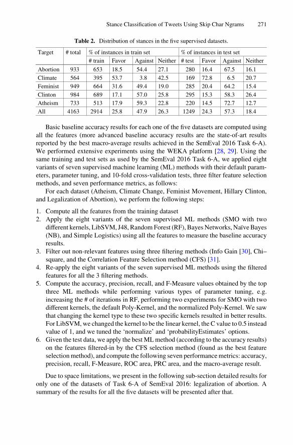
Table 2. Distribution of stances in the five supervised datasets.
Target # total % of instances in train set % of instances in test set# train Favor Against Neither # test Favor Against Neither
Abortion 933 653 18.5 54.4 27.1 280 16.4 67.5 16.1Climate 564 395 53.7 3.8 42.5 169 72.8 6.5 20.7Feminist 949 664 31.6 49.4 19.0 285 20.4 64.2 15.4Clinton 984 689 17.1 57.0 25.8 295 15.3 58.3 26.4Atheism 733 513 17.9 59.3 22.8 220 14.5 72.7 12.7All 4163 2914 25.8 47.9 26.3 1249 24.3 57.3 18.4
Basic baseline accuracy results for each one of the five datasets are computed usingall the features (more advanced baseline accuracy results are the state-of-art resultsreported by the best macro-average results achieved in the SemEval 2016 Task 6-A).We performed extensive experiments using the WEKA platform [28, 29]. Using thesame training and test sets as used by the SemEval 2016 Task 6-A, we applied eightvariants of seven supervised machine learning (ML) methods with their default param‐eters, parameter tuning, and 10-fold cross-validation tests, three filter feature selectionmethods, and seven performance metrics, as follows:
For each dataset (Atheism, Climate Change, Feminist Movement, Hillary Clinton,and Legalization of Abortion), we perform the following steps:
1. Compute all the features from the training dataset2. Apply the eight variants of the seven supervised ML methods (SMO with two
different kernels, LibSVM, J48, Random Forest (RF), Bayes Networks, Naïve Bayes(NB), and Simple Logistics) using all the features to measure the baseline accuracyresults.
3. Filter out non-relevant features using three filtering methods (Info Gain [30], Chi–square, and the Correlation Feature Selection method (CFS) [31].
4. Re-apply the eight variants of the seven supervised ML methods using the filteredfeatures for all the 3 filtering methods.
5. Compute the accuracy, precision, recall, and F-Measure values obtained by the topthree ML methods while performing various types of parameter tuning, e.g.increasing the # of iterations in RF, performing two experiments for SMO with twodifferent kernels, the default Poly-Kernel, and the normalized Poly-Kernel. We sawthat changing the kernel type to these two specific kernels resulted in better results.For LibSVM, we changed the kernel to be the linear kernel, the C value to 0.5 insteadvalue of 1, and we tuned the ‘normalize’ and ‘probabilityEstimates’ options.
6. Given the test data, we apply the best ML method (according to the accuracy results)on the features filtered-in by the CFS selection method (found as the best featureselection method), and compute the following seven performance metrics: accuracy,precision, recall, F-Measure, ROC area, PRC area, and the macro-average result.
Due to space limitations, we present in the following sub-section detailed results foronly one of the datasets of Task 6-A of SemEval 2016: legalization of abortion. Asummary of the results for all the five datasets will be presented after that.
Stance Classification of Tweets Using Skip Char Ngrams 271
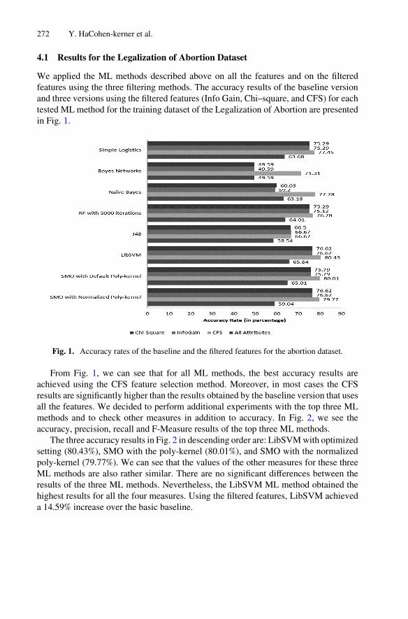
4.1 Results for the Legalization of Abortion Dataset
We applied the ML methods described above on all the features and on the filteredfeatures using the three filtering methods. The accuracy results of the baseline versionand three versions using the filtered features (Info Gain, Chi–square, and CFS) for eachtested ML method for the training dataset of the Legalization of Abortion are presentedin Fig. 1.
Fig. 1. Accuracy rates of the baseline and the filtered features for the abortion dataset.
From Fig. 1, we can see that for all ML methods, the best accuracy results areachieved using the CFS feature selection method. Moreover, in most cases the CFSresults are significantly higher than the results obtained by the baseline version that usesall the features. We decided to perform additional experiments with the top three MLmethods and to check other measures in addition to accuracy. In Fig. 2, we see theaccuracy, precision, recall and F-Measure results of the top three ML methods.
The three accuracy results in Fig. 2 in descending order are: LibSVM with optimizedsetting (80.43%), SMO with the poly-kernel (80.01%), and SMO with the normalizedpoly-kernel (79.77%). We can see that the values of the other measures for these threeML methods are also rather similar. There are no significant differences between theresults of the three ML methods. Nevertheless, the LibSVM ML method obtained thehighest results for all the four measures. Using the filtered features, LibSVM achieveda 14.59% increase over the basic baseline.
272 Y. HaCohen-kerner et al.
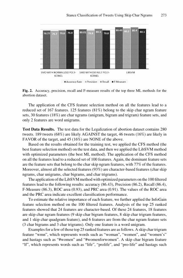
Fig. 2. Accuracy, precision, recall and F-measure results of the top three ML methods for theabortion dataset.
The application of the CFS feature selection method on all the features lead to areduced set of 167 features. 125 features (81%) belong to the skip char ngram featuresets, 30 features (18%) are char ngrams (unigram, bigram and trigram) feature sets, andonly 2 features are word unigrams.
Test Data Results. The test data for the Legalization of abortion dataset contains 280tweets. 189 tweets (68%) are likely AGAINST the target, 46 tweets (16%) are likely inFAVOR of the target, and 45 (16%) are NONE of the above.
Based on the results obtained for the training test, we applied the CFS method (thebest feature selection method) on the test data, and then we applied the LibSVM methodwith optimized parameters (the best ML method). The application of the CFS methodon all the features lead to a reduced set of 100 features. Again, the dominant feature setsare the feature sets that belong to the char skip ngram features, with 77% of the features.Moreover, almost all the selected features (93%) are character-based features (char skipngrams, char unigrams, char bigrams, and char trigrams).
The application of the LibSVM method with optimized parameters on the 100 filteredfeatures lead to the following results: accuracy (86.43), Precision (86.2), Recall (86.4),F-Measure (86.3), ROC area (0.93), and PRC area (0.91). The values of the ROC areaand the PRC area indicate excellent classification performance.
To estimate the relative importance of each feature, we further applied the InfoGainfeature selection method on the 100 filtered features. Analysis of the top 25 rankedfeatures showed that 24 features are character-based. Of these 24 features, 18 featuresare skip char ngram features (9 skip char bigram features, 8 skip char trigram features,and 1 skip char quadgram feature), and 6 features are from the char ngram feature sets(3 char bigrams and 3 char trigrams). Only one feature is a word unigram.
Examples for a few of those top 25 ranked features are as follows. A skip char trigramfeature “wmn”, which represents words such as “woman”, “women”, and “women’s”and hastags such as “#women” and “#womenforwomen”. A skip char bigram feature“lf”, which represents words such as “life”, “prolife”, and “pro-life” and hastags such
Stance Classification of Tweets Using Skip Char Ngrams 273

as “#everylifematters” and “#ProLifeYouth”. A char bigram “wo”, which is commonto some frequent relevant words and hastags such as “woman”, “women”, “women’s”,“#women”, and “work”, and also of non-relevant frequent words such as “would”. Theonly word unigram, which is among the top ranked features is “men”, a group of peoplewhich also has what to tweet about abortion.
The main conclusion from these results is that most of the top features are characterngrams and skip character ngrams. These features serve as generalized features thatinclude within them semantically close words and hastags, and their declensions. Thesefeatures allow to overcome problems such as noise and sparse data and enable successfulclassification.
Comparison to the Contest Results. In the contest, organized by the SemEval 2016 Task6-A [14] for all the test datasets, the organizers used the macro-average measure as theevaluation metric for the task. The macro-average (also called Favg) is defined as:
Favg = (Ffavor + Fagainst) ∕ 2 (1)
where Ffavor and Fagainst are defined as follows:
Ffavor = 2PfavorRfavor ∕ (Pfavor + Rfavor) (2)
Fagainst = 2PagainstRagainst∕ (Pagainst + Ragainst) (3)
Our results were: Fagainst = 90.7, Ffavor = 73.8, and Favg = 82.25. The score of82.25 is significantly higher than the Favg results of all the 19 competitors, includingthe best Favg result (66.42) obtained by the baseline SVM-ngrams team using all thepossible word ngrams (this team was not a part of the official competition) and the bestFavg result (63.32) achieved by the DeepStance team (a part of the official competition)using ngrams, word embedding vectors, sentiment analysis features such as those drawnfrom sentiment lexicons [32], and stance bearing hashtags.
In contrast to the Favg scores of many of the competitors of the SemEval 2016 Task6-A, that were obtained using thousands of ngrams and hundreds of word embeddingfeatures, our Favg score is significantly better mainly probably due to the use of the CFSfeature selection method and the use of only 100 derived features where 93 of them arecharacter-based features and 77 of them are skip char ngram features.
4.2 Summary of the Results for All Five Datasets
Table 3 presents a summary of the results of our algorithm for all the five test datasetsand Table 4 presents a comparison of the Favg values and an analysis of our features.
General findings that can be derived from Table 3 are: (1) The best ML methods arethe two SVM’s versions and Naïve Bayes; (2) The best filtering method is CFS; (3) Thenumber of the filtered features is relatively very small (between 53 to 111); and (4) Thevalues of all measures are relatively high (around 85% and up) for all test datasets.
274 Y. HaCohen-kerner et al.
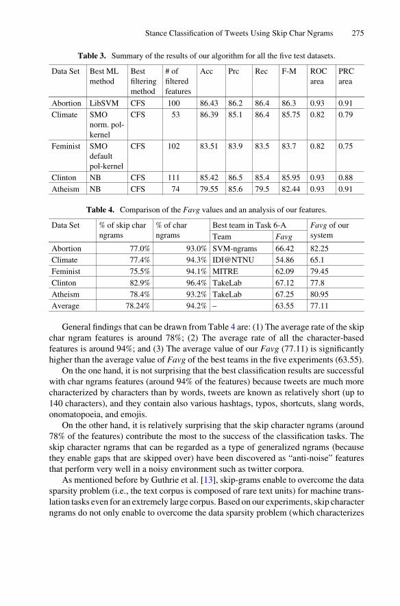
Table 4. Comparison of the Favg values and an analysis of our features.
Data Set % of skip charngrams
% of charngrams
Best team in Task 6-A Favg of oursystemTeam Favg
Abortion 77.0% 93.0% SVM-ngrams 66.42 82.25Climate 77.4% 94.3% IDI@NTNU 54.86 65.1Feminist 75.5% 94.1% MITRE 62.09 79.45Clinton 82.9% 96.4% TakeLab 67.12 77.8Atheism 78.4% 93.2% TakeLab 67.25 80.95Average 78.24% 94.2% – 63.55 77.11
General findings that can be drawn from Table 4 are: (1) The average rate of the skipchar ngram features is around 78%; (2) The average rate of all the character-basedfeatures is around 94%; and (3) The average value of our Favg (77.11) is significantlyhigher than the average value of Favg of the best teams in the five experiments (63.55).
On the one hand, it is not surprising that the best classification results are successfulwith char ngrams features (around 94% of the features) because tweets are much morecharacterized by characters than by words, tweets are known as relatively short (up to140 characters), and they contain also various hashtags, typos, shortcuts, slang words,onomatopoeia, and emojis.
On the other hand, it is relatively surprising that the skip character ngrams (around78% of the features) contribute the most to the success of the classification tasks. Theskip character ngrams that can be regarded as a type of generalized ngrams (becausethey enable gaps that are skipped over) have been discovered as “anti-noise” featuresthat perform very well in a noisy environment such as twitter corpora.
As mentioned before by Guthrie et al. [13], skip-grams enable to overcome the datasparsity problem (i.e., the text corpus is composed of rare text units) for machine trans‐lation tasks even for an extremely large corpus. Based on our experiments, skip characterngrams do not only enable to overcome the data sparsity problem (which characterizes
Table 3. Summary of the results of our algorithm for all the five test datasets.
Data Set Best MLmethod
Bestfilteringmethod
# offilteredfeatures
Acc Prc Rec F-M ROCarea
PRCarea
Abortion LibSVM CFS 100 86.43 86.2 86.4 86.3 0.93 0.91Climate SMO
norm. pol-kernel
CFS 53 86.39 85.1 86.4 85.75 0.82 0.79
Feminist SMOdefaultpol-kernel
CFS 102 83.51 83.9 83.5 83.7 0.82 0.75
Clinton NB CFS 111 85.42 86.5 85.4 85.95 0.93 0.88Atheism NB CFS 74 79.55 85.6 79.5 82.44 0.93 0.91
Stance Classification of Tweets Using Skip Char Ngrams 275

short text corpora) but also help to overcome noisy problems (e.g., misspellings, onoma‐topoeia, replicated characters, and slang words), which also characterize short textcorpora.
5 Summary, Conclusions and Future Work
In this study, we present an implementation of stance classification tasks based mainlyon a limited number of features, which contain mainly char ngrams features in generaland char skip ngrams in particular. To the best of our knowledge, we are the first toperform successful stance classification using mainly skip character ngrams.
The macro-average results obtained by our algorithm are significantly higher thanthe state-of-art results reported by the best macro-average results achieved in theSemEval 2016 Task 6-A [14] for all the five released datasets of tweets in the frameworkof task-A (the supervised framework).
In contrast to the competitors of the SemEval 2016 Task 6-A, that did not use anychar skip ngrams but rather used thousands of ngrams and hundreds of word embeddingfeatures, our algorithm uses a limited number of features (53–111) derived by the CFSselection method, mainly character-based features where most of them are skip charngram features.
Our experiments show that two feature sets are very helpful for stance classificationof tweets: (1) char ngrams features in general probably because tweets are much morecharacterized by characters than by words, tweets are relatively short (up to 140 char‐acters), and contain also various typos, shortcuts, hashtags, slang words, onomatopoeia,and emojis and (2) skip character ngrams in particular probably because they serve asgeneralized ngrams that allow to overcome problems such as noise and sparse data.
In order to examine the usefulness of character ngrams in general and skip characterngrams in particular we suggest the following future research proposals: conductingadditional experiments for larger social corpora of various types of short text files writtenin various languages based on more feature sets and applying additional supervised MLmethods such as deep learning methods.
Acknowledgments. The authors thank three anonymous reviewers for their help and fruitfulcomments.
References
1. Liu, B., Zhang, L.: A survey of opinion mining and sentiment analysis. In: Aggarwal, C.,Zhai, C. (eds.) Mining Text Data, pp. 415–463. Springer, Boston (2012). https://doi.org/10.1007/978-1-4614-3223-4_13
2. Mohammad, S.M., Zhu, X., Kiritchenko, S., Martin, J.: Sentiment, emotion, purpose, andstyle in electoral tweets. Inf. Process. Manage. 51(4), 480–499 (2015)
3. Basave, C., He, A.E., He, Y., Liu, K., Zhao, J.: A weakly supervised bayesian model forviolence detection in social media (2013)
276 Y. HaCohen-kerner et al.

4. Somasundaran, S., Wiebe, J.: Recognizing stances in ideological on-line debates. In:Proceedings of the NAACL HLT 2010 Workshop on Computational Approaches to Analysisand Generation of Emotion in Text, pp. 116–124. Association for Computational Linguistics(2010)
5. Murakami, A., Raymond, R.: Support or oppose? Classifying positions in online debates fromreply activities and opinion expressions. In: Proceedings of the 23rd International Conferenceon Computational Linguistics: Posters, pp. 869–875. Association for ComputationalLinguistics (2010)
6. Anand, P., Walker, M., Abbott, R., Tree, J.E.F., Bowmani, R., Minor, M.: Cats rule and dogsdrool!: classifying stance in online debate. In Proceedings of the 2nd Workshop onComputational Approaches to Subjectivity and Sentiment Analysis, pp. 1–9. Association forComputational Linguistics (2011)
7. Sridhar, D., Foulds, J., Huang, B., Getoor, L., Walker, M.: Joint models of disagreement andstance in online debate. In: Annual Meeting of the Association for Computational Linguistics(2015)
8. Thomas, M., Pang, B., Lee, L.: Get out the vote: determining support or opposition fromCongressional floor-debate transcripts. In: Proceedings of the 2006 Conference on EmpiricalMethods in Natural Language Processing, pp. 327–335. Association for ComputationalLinguistics (2006)
9. Yessenalina, A., Yue, Y., Cardie, C.: Multi-level structured models for document-levelsentiment classification. In: Proceedings of EMNLP, pp. 1046–1056 (2010)
10. Burfoot, C., Bird, S., Baldwin, T.: Collective classification of congressional floor-debatetranscripts. In: Proceedings of the 49th Annual Meeting of the Association for ComputationalLinguistics: Human Language Technologies-Volume 1, pp. 1506–1515. Association forComputational Linguistics (2011)
11. Agrawal, R., Rajagopalan, S., Srikant, R., Xu, Y.: Mining newsgroups using networks arisingfrom social behavior. In: Proceedings of WWW, pp. 529–535 (2003)
12. Rajendran, P., Bollegala, D., Parsons, S.: Contextual stance classification of opinions: a steptowards enthymeme reconstruction in online reviews. In: Proceedings of the 3rd Workshopon Argument Mining, pp. 31–39. Association for Computational Linguistics, Berlin (2016)
13. Guthrie, D., Allison, B., Liu, W., Guthrie, L., Wilks, Y.: A closer look at skip-gram modelling.In: Proceedings of the 5th International Conference on Language Resources and Evaluation(LREC-2006), pp. 1222–1225 (2006)
14. Mohammad, S.M., Kiritchenko, S., Sobhani, P., Zhu, X., Cherry, C.: SemEval-2016 task 6:detecting stance in tweets. In: Proceedings of SemEval, pp. 31–41 (2016)
15. Xu, R., Zhou, Yu., Wu, D., Gui, L., Du, J., Xue, Y.: Overview of NLPCC Shared Task 4:stance detection in Chinese microblogs. In: Lin, C.-Y., Xue, N., Zhao, D., Huang, X., Feng,Y. (eds.) ICCPOL/NLPCC -2016. LNCS (LNAI), vol. 10102, pp. 907–916. Springer, Cham(2016). https://doi.org/10.1007/978-3-319-50496-4_85
16. Jans, B., Bethard, S., Vulić, I., Moens, M.F.: Skip n-grams and ranking functions forpredicting script events. In: Proceedings of the 13th Conference of the European Chapter ofthe Association for Computational Linguistics, pp. 336–344. Association for ComputationalLinguistics (2012)
17. Sidorov, G., Velasquez, F., Stamatatos, E., Gelbukh, A., Chanona-Hernández, L.: Syntacticn-grams as machine learning features for natural language processing. Expert Syst. Appl.41(3), 853–860 (2014)
18. Fernández, J., Gutiérrez, Y., Gómez, J.M., Martınez-Barco, P.: GPLSI: supervised sentimentanalysis in twitter using skipgrams. In: Proceedings of the 8th International Workshop onSemantic Evaluation (SemEval 2014), number SemEval, pp. 294–299 (2014)
Stance Classification of Tweets Using Skip Char Ngrams 277

19. Dhondt, E., Verberne, S., Weber, N., Koster, C., Boves, L.: Using skipgrams and pos-basedfeature selection for patent classification. Comput. Linguist. Neth. J. 2, 52–70 (2012)
20. HaCohen-Kerner, Y., Beck, H., Yehudai, E., Rosenstein, M., Mughaz, D.: Cuisine:classification using stylistic feature sets and/or name-based feature sets. J. Am. Soc. Inform.Sci. Technol. 61(8), 1644–1657 (2010)
21. HaCohen-Kerner, Y., Beck, H., Yehudai, E., Mughaz, D.: Stylistic feature sets as classifiersof documents according to their historical period and ethnic origin. Appl. Artif. Intell. 24(9),847–862 (2010)
22. Mohammad, S.M., Kiritchenko, S., Zhu, X.: National Research Council Canada (NRC) Hashtagunigram Lexicon (2013). http://saifmohammad.com/WebPages/SCL.html. Accessed 18 Apr 2017
23. https://www.cs.uic.edu/~liub/FBS/sentiment-analysis.html. Accessed 18 Apr 201724. http://mpqa.cs.pitt.edu/lexicons/subj_lexicon/. Accessed 18 Apr 201725. https://www.ling.upenn.edu/courses/Fall_2003/ling001/penn_treebank_pos.html. Accessed
18 Apr 201726. http://nlp.stanford.edu/software/tagger.shtml. Accessed 18 Apr 201727. Klein, D., Manning, C.D.: Accurate unlexicalized parsing. In: Proceedings of the 41st Annual
Meeting on Association for Computational Linguistics, vol. 1, pp. 423–430. Association forComputational Linguistics (2003)
28. Witten, I.H., Frank, E.: Data Mining: Practical Machine Learning Tools and Techniques, 2ndedn. Morgan Kaufmann Series in Data Management Systems. Morgan Kaufmann, San Mateo(2005)
29. Hall, M.: Correlation-based feature selection for machine learning. Doctoral dissertation, TheUniversity of Waikato (1999)
30. Yang, Y., Pedersen, J.O.: A comparative study on feature selection in text categorization. In:Icml, pp. 412–420 (1997)
31. Hall, M., Frank, E., Holmes, G., Pfahringer, B., Reutemann, P., Witten, I.H.: The WEKAdata mining software. ACM SIGKDD Explor. Newsl. 11(1), 10 (2009)
32. Kiritchenko, S., Zhu, X., Mohammad, S.M.: Sentiment analysis of short informal texts. J.Artif. Intell. Res. 50, 723–762 (2014)
278 Y. HaCohen-kerner et al.

Structural Semantic Models for AutomaticAnalysis of Urban Areas
Gianni Barlacchi1,2(B), Alberto Rossi3, Bruno Lepri3,and Alessandro Moschitti1,4
1 University of Trento, Trento, [email protected], [email protected]
2 SKIL - Telecom Italia, Trento, Italy3 Bruno Kessler Foundation (FBK), Trento, Italy
{alrossi,lepri}@fbk.eu4 Qatar Computing Research Institute, HBKU, Doha, Qatar
Abstract. The growing availability of data from cities (e.g., traffic flow,human mobility and geographical data) open new opportunities for pre-dicting and thus optimizing human activities. For example, the auto-matic analysis of land use enables the possibility of better administrat-ing a city in terms of resources and provided services. However, suchanalysis requires specific information, which is often not available forprivacy concerns. In this paper, we propose a novel machine learningrepresentation based on the available public information to classify themost predominant land use of an urban area, which is a very commontask in urban computing. In particular, in addition to standard featurevectors, we encode geo-social data from Location-Based Social Networks(LBSNs) into a conceptual tree structure that we call Geo-Tree. Then,we use such representation in kernel machines, which can thus performaccurate classification exploiting hierarchical substructure of concepts asfeatures. Our extensive comparative study on the areas of New Yorkand its boroughs shows that Tree Kernels applied to Geo-Trees are veryeffective improving the state of the art up to 18% in Macro-F1.
1 Introduction
The demographic trend clearly shows an increasing concentration of people inhuge cities. By 2030, 9% of the world population is expected to live in just41 mega-cities, each one with more than 10M inhabitants. Thus, the growingavailability of data [2] makes it possible to discover new interesting aspects aboutcities and its life at a fine unprecedented granularity.
A fundamental challenge that policy makers and urban planners are dealingwith is land use classification, which plays an important role for infrastructureplanning and development, real-estate evaluations, and authorizations of busi-ness permits. More in detail, policy makers and urban planners need to associatedifferent urban areas with specific human activities (e.g., residential, industrial,business, nightlife and others). However, traditional survey-based approachesc© Springer International Publishing AG 2017Y. Altun et al. (Eds.): ECML PKDD 2017, Part III, LNAI 10536, pp. 279–291, 2017.https://doi.org/10.1007/978-3-319-71273-4_23
280 G. Barlacchi et al.
to classify areas are time consuming and very costly to be applied to modernhuge cities. Therefore, automatic approaches using novel sources of data (e.g.,data from mobile phones, LBSNs, etc.) have been proposed. For example, [19]designed supervised and unsupervised approaches to infer New York City (NYC)land use from check-in. A check-in usually consists of latitude and longitude coor-dinates associated with additional metadata such as the venue where the userchecked-in, comments and photos. Such data can be extracted from LBSNs likeFoursquare1, a social network application that provides the number and typeof activities present in the target area (e.g., Arts & Entertainment, NightlifeSpot, etc.). The approach basically used feature vectors, mainly consisting of thenumber of check-in with the associated activity inferred from the Foursquarecategory of the place (e.g., eating if the check-in is done in a restaurant). AsGold Standard, the authors used data provided by the NYC Department of CityPlanning in 2013 mapped on a grid of 200× 200 m.
In this paper, we represent geographical areas in two different ways: (i) asa bag-of-concepts (BOC), e.g., Arts and Entertainment, College and University,Event, Food extracted from the Foursquare description of the area; and (ii) asthe same concepts above organized in a tree, reflecting the hierarchical categorystructure of Foursquare activities. We designed kernels combining BOC vectorswith Tree Kernels (TKs) [6,9,10,17] applied to concept trees and used them inSupport Vector Machines (SVMs). This way, our model (i) can learn complexstructural and semantic patterns encoded in our hierarchical conceptualization ofan area and (ii) highly improves the accuracy of standard classification methodsbased on BOC. Our GeoTK represents an interesting novelty as we show thatTKs not only can capture semantic information from natural language text,e.g., as shown for semantic role labeling [12] and question answering [3,15], butthey can also convey conceptual features from the hierarchy above to performsemantic inference, such as deciding which is the major activity of a land. Ourapproach is largely applicable as (i) it can use any hierarchical category structurefor POIs categories (e.g., OpenStreet Map POIs data); and (ii) many cities offeropen access to their land use data.
Finally, we carry out a study with different granularities of the areas to beanalyzed. This also enables to analyze the trade-off between the precision intargeting the area of interest and the accuracy with which we carry out theestimation. More in detail, we divide the NYC area in squares with edges of50, 100, 200 and 250 m and, for each cell, we classify its most predominant landuse class (e.g., Residential, Commercial, Manufacturing, etc.). Our extensiveexperimentation, including a comparative study as well as the use of severalmachine learning models, shows that GeoTKs are very effective and improve thestate of the art up to 18% in Macro-F1.
The reminder of this paper is organized as follows, Sect. 2 introduces therelated work, Sect. 3 describes the task and the related data, Sect. 4 presents
1 https://foursquare.com.

Structural Semantic Models for Automatic Analysis of Urban Areas 281
our hierarchical tree representation and our GeoTK. Then, Sect. 5 illustrates theevaluation of our approach, and finally Sect. 6 derives some conclusions.
2 Related Work
Several works have targeted land use inference by means of different sources ofinformation. For example, [18] built a framework that, using human mobilitypatterns derived from taxicab trajectories and Point Of Interests (POIs), classi-fies the functionality of an area for the city of Beijing. The model is similar to theone used for topic discovery in a textual document, where the functionality ofan area is the topic, the region is the document, and POIs and mobility patternsare metadata and words, respectively. Specifically, [18] have used an advancedmodel combining Latent Dirichlet Allocation (LDA) with Dirichlet MultinomialRegression (DMR), in order to insert also information coming from the POIs(metadata). Hence, for each region, after the parameter estimation with DMR,they have a vector representing the intensity of each topic. This vector is thenused to aggregate formal regions having similar functions by k-means clustering.
Similarly, [1] proposed a spatio-temporal approach for the detection of func-tional regions. They exploited three different clustering algorithms by using dif-ferent set of features extracted from Foursquare’s POIs and check-in activities inManhattan (New York). This task permits to better understand how the func-tionality of a city’s region changes over time. Other works have used geo-taggeddata from social networks: for example, [8] used tweets as input data to predictthe land use of a certain area of Manhattan. Moreover, they try to infer POIsfrom tweets’ patterns clustering the surface with Self-Organizing-Map, then char-acterizing each region with a specific tweet pattern and finally using k-means toinfer land use. Again, [19] have used check-in data to compare unsupervised andsupervised approaches to land use inference.
Finally, some works have also used Call Detail Records (CDRs) [7,8,13,16],which are typically used by mobile phone operators for billing purposes. Thisdata registers the time and type of the communication (e.g., incoming calls, Inter-net, outgoing SMS), and the radio base station handling the communication. Forexample, [16] have used CDRs jointly with a Random Forest classifier to build atime-varying land use classification for the city of Boston. The intuition behindthis work is to mine a time-variant relation between movement patterns andland use. In particular, they perform a Random Forest prediction and then theycompare it with the predictions obtained for the neighboring regions, applyinga sort of consensus validation (e.g., they modify the prediction if a certain num-ber of neighbors belong to a different uniform function). This way, they modeldifferent land uses for different temporal slots of the day.
Compared to the state of the art, the main novelties introduced by ourwork are the following: (i) we model the hierarchical semantic information ofFoursquare using GeoTK, thus adding powerful structural features in our clas-sification models; and (ii) we study how the size of the grid impacts on theaccuracy of different models, thus investigating the trade-off between granular-ity of the analysis and accuracy. It should be also noted that, in contrast to

282 G. Barlacchi et al.
previous work, GeoTK does not rely on external resources (e.g., mobile phonedata) or heavy features engineering in addition to the structural kernel model.
3 Datasets
We use the shape file of New York provided by the NYC government2. Thisfile is publicly available and contains the entire shape of New York divided inthe 5 boroughs: Manhattan, Brooklyn, Staten Island, Bronx, and Queens. Then,we build a grid over the entire city in order to enable our classification task.The goal is to infer the land use of a region given a target label and a featurerepresentation of the region. In the next subsections, we describe (i) the land usedata and labels utilized by our approach, and (ii) the Foursquare’s POIs usedto obtain a feature representation of the land of a region.
3.1 Land Use
In our study, we use MapPluto, a freely available dataset provided by the NYCgovernment, which contains precise geo-referenced information for each city’sborough. For example, it provides the precise category and shape for each build-ing in the city (Fig. 1). More in detail, it contains the following land use cate-gories: (i) One and Two Family Buildings, (ii) Multi-Family Walk-Up Buildings,(iii) Multi-Family Elevator Buildings, (iv) Mixed Residential and CommercialBuildings, (v) Commercial and Office Buildings, (vi) Industrial and Manufac-turing Buildings, (vii) Transportation and Utility, (viii) Public Facilities andInstitutions, (ix) Open Space and Outdoor Recreation, (x) Parking Facilities,and (xi) Vacant Land. Land use information is very fine-grained, and in mostcases there is only one land use assigned to one building, thus making it very diffi-cult to determine the land use with just POI information. A reasonable trade-offbetween classification accuracy and the desired area granularity consists in seg-menting the regions in squared cells: each cell will refer to more than one landuse but we consider the predominant class as its primary use.
3.2 Foursquare’s Point of Interests
We extracted 206,602 POIs from the entire NYC. As for the land use data, wehave several sources of information, but we focused on the ten macro-categoriesof the POIs, each one specialized in maximum four levels of detail. These levelsfollow a hierarchical structure3, where each level of a category has a finite num-ber of subcategories as node children. For instance, the first level of POIs maincategories is constituted by: (i) Arts and Entertainment, (ii) College and Uni-versity, (iii) Event, (iv) Food, (v) Nightlife Spot, (vi) Outdoors and Recreation,
2 http://www1.nyc.gov/site/planning/data-maps/open-data/districts-download-metadata.page.
3 https://developer.foursquare.com/categorytree.

Structural Semantic Models for Automatic Analysis of Urban Areas 283
Fig. 1. Example of land use distribution in New York City.
(vii) Professional and Other Places, (viii) Residence, (ix) Shop and Service, and(x) Travel and Transport. The second level includes 437 categories whereas thethird level contains a smaller number of categories, 345.
4 Semantic Structural Models for Land Use Analysis
Previous works [4,13,14] have mainly used features extracted from LBSNs (e.g.,Foursquare’s POIs) in the XGboost algorithm [5]. However, these feature vectorshave several limitations such as (i) the small amount of information available forthe target area and (ii) their inherent scalar nature, which does not capture theexistence and the type of relations between different POIs. Here, we propose amuch powerful approach based on TKs applied to a semantic structure based onthe hierarchical organization of the Foursquare categories.
4.1 Bag-of-Concepts
The most straightforward way to represent an area by means of Foursquaredata is to use its POIs. Every venue is hierarchically categorized (e.g., Profes-sional and Other Places → Medical Center → Doctor’s office) and the categoriesare used to produce an aggregated representation of the area. We use this fea-ture representation by aggregating all the venues together, namely we count themacro-level category (e.g., Food) in all the POIs that we found in any cell grid.This way, we generate the Bag-Of-Concepts (BOC) feature vectors, counting thenumber of each activity under each macro-category.
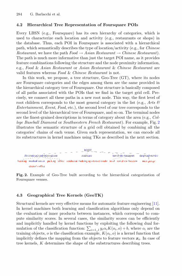
284 G. Barlacchi et al.
4.2 Hierarchical Tree Representation of Foursquare POIs
Every LBSN (e.g., Foursquare) has its own hierarchy of categories, which isused to characterize each location and activity (e.g., restaurants or shops) inthe database. Thus, each POI in Foursquare is associated with a hierarchicalpath, which semantically describes the type of location/activity (e.g., for ChineseRestaurant, we have the path Food → Asian Restaurant → Chinese Restaurant).The path is much more informative than just the target POI name, as it providesfeature combinations following the structure and the node proximity information,e.g., Food & Asian Restaurant or Asian Restaurant & Chinese Restaurant arevalid features whereas Food & Chinese Restaurant is not.
In this work, we propose, a tree structure, Geo-Tree (GT), where its nodesare Foursquare categories and the edges among them are the same provided inthe hierarchical category tree of Foursquare. Our structure is basically composedof all paths associated with the POIs that we find in the target grid cell. Pre-cisely, we connect all these paths in a new root node. This way, the first level ofroot children corresponds to the most general category in the list (e.g., Arts &Entertainment, Event, Food, etc.), the second level of our tree corresponds to thesecond level of the hierarchical tree of Foursquare, and so on. The terminal nodesare the finest-grained descriptions in terms of category about the area (e.g., Col-lege Baseball Diamond or Southwestern French Restaurant). For example, Fig. 2illustrates the semantic structure of a grid cell obtained by combining all thecategories’ chains of each venue. Given such representation, we can encode allits substructures in kernel machines using TKs as described in the next section.
Fig. 2. Example of Geo-Tree built according to the hierarchical categorization ofFoursquare venues.
4.3 Geographical Tree Kernels (GeoTK)
Structural kernels are very effective means for automatic feature engineering [11].In kernel machines both learning and classification algorithms only depend onthe evaluation of inner products between instances, which correspond to com-pute similarity scores. In several cases, the similarity scores can be efficientlyand implicitly handled by kernel functions by exploiting the following dual for-mulation of the classification function:
∑i=1..l yiαiK(oi, o) + b, where oi are the
training objects, o is the classification example, K(oi, o) is a kernel function thatimplicitly defines the mapping from the objects to feature vectors xi . In case oftree kernels, K determines the shape of the substructures describing trees.

Structural Semantic Models for Automatic Analysis of Urban Areas 285
4.4 Tree Kernels
In the majority of machine learning approaches, data examples are transformedin feature vectors, which in turn are used in dot products for carrying out bothlearning and classification steps. Kernel Machines (KMs) allow for replacing thedot product with kernel functions, which compute the dot product directly fromexamples (i.e., they avoid the transformation of examples in vectors).
Given two input trees, TKs evaluate the number of substructures, also calledfragments, that they have in common. More formally, let F = {f1, f2, . . . ..fF}be the space of all possible tree fragments and χi(n) an indicator function suchthat it is equal to 1 if the target f1 is rooted in n, equal to 0 otherwise. TKs overT1 and T2 are defined by TK(T1, T2) =
∑n1∈NT1
∑n2∈NT2
Δ(n1, n2), where NT1
e NT2 are the set of nodes of T1 and T2 and
Δ(n1, n2) =F∑
i=1
χi(n1)χi(n2) (1)
represents the number of common fragments rooted at nodes n1 and n2. Thenumber and the type of fragments generated depends on the type of the usedtree kernel functions, which, in turn, depends on Δ(n1, n2).
Syntactic Tree Kernels (STK). Its computation is carried out by usingΔSTK(n1, n2) in Eq. 1 defined as follows (in a syntactic tree, each node can beassociated with a production rule):
(i) if the productions at n1 and n2 are different ΔSTK(n1, n2) = 0;(ii) if the productions at n1 and n2 are the same, and n1 and n2 have
only leaf children then ΔSTK(n1, n2) = λ; and(iii) if the productions at n1 and n2 are the same, and n1 and n2 are
not pre-terminals then ΔSTK(n1, n2) = λ∏l(n1)
j=1 (1 + ΔSTK(cjn1, cjn2
)),
where l(n1) is the number of children of n1 and cjn is the j-th child of thenode n. Note that, since the productions are the same, l(n1) = l(n2) and thecomputational complexity of STK is O(|NT1 ||NT2 |) but the average running timetends to be linear, i.e., O(|NT1 |+|NT2 |), for natural language syntactic trees [10].
Finally, by adding the following step:
(0) if the nodes n1 and n2 are the same then ΔSTK(n1, n2) = λ,
also the individual nodes will be counted by ΔSTK . We call this kernel STKb.
The Partial Tree Kernel (PTK). [10] generalizes a large class of tree ker-nels as it computes one of the most general tree substructure spaces. Given twotrees, PTK considers any connected subset of nodes as possible features of thesubstructure space. Its computation is carried out by Eq. 1 using the followingΔPTK function:
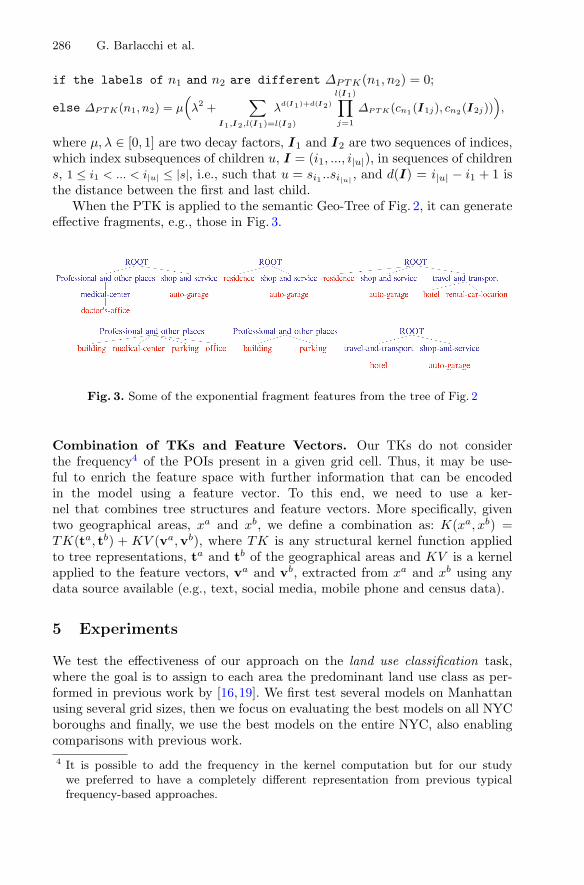
286 G. Barlacchi et al.
if the labels of n1 and n2 are different ΔPTK(n1, n2) = 0;
else ΔPTK(n1, n2) = μ(λ2 +
∑
I1,I2,l(I1)=l(I2)
λd(I 1)+d(I 2)
l(I1)∏
j=1
ΔPTK(cn1(I1j), cn2(I2j))),
where μ, λ ∈ [0, 1] are two decay factors, I1 and I2 are two sequences of indices,which index subsequences of children u, I = (i1, ..., i|u|), in sequences of childrens, 1 ≤ i1 < ... < i|u| ≤ |s|, i.e., such that u = si1 ..si|u| , and d(I) = i|u| − i1 + 1 isthe distance between the first and last child.
When the PTK is applied to the semantic Geo-Tree of Fig. 2, it can generateeffective fragments, e.g., those in Fig. 3.
Fig. 3. Some of the exponential fragment features from the tree of Fig. 2
Combination of TKs and Feature Vectors. Our TKs do not considerthe frequency4 of the POIs present in a given grid cell. Thus, it may be use-ful to enrich the feature space with further information that can be encodedin the model using a feature vector. To this end, we need to use a ker-nel that combines tree structures and feature vectors. More specifically, giventwo geographical areas, xa and xb, we define a combination as: K(xa, xb) =TK(ta, tb) + KV (va,vb), where TK is any structural kernel function appliedto tree representations, ta and tb of the geographical areas and KV is a kernelapplied to the feature vectors, va and vb, extracted from xa and xb using anydata source available (e.g., text, social media, mobile phone and census data).
5 Experiments
We test the effectiveness of our approach on the land use classification task,where the goal is to assign to each area the predominant land use class as per-formed in previous work by [16,19]. We first test several models on Manhattanusing several grid sizes, then we focus on evaluating the best models on all NYCboroughs and finally, we use the best models on the entire NYC, also enablingcomparisons with previous work.4 It is possible to add the frequency in the kernel computation but for our study
we preferred to have a completely different representation from previous typicalfrequency-based approaches.
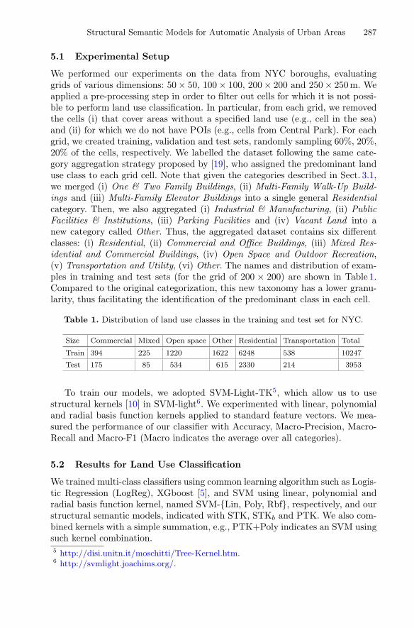
Structural Semantic Models for Automatic Analysis of Urban Areas 287
5.1 Experimental Setup
We performed our experiments on the data from NYC boroughs, evaluatinggrids of various dimensions: 50 × 50, 100 × 100, 200 × 200 and 250 × 250 m. Weapplied a pre-processing step in order to filter out cells for which it is not possi-ble to perform land use classification. In particular, from each grid, we removedthe cells (i) that cover areas without a specified land use (e.g., cell in the sea)and (ii) for which we do not have POIs (e.g., cells from Central Park). For eachgrid, we created training, validation and test sets, randomly sampling 60%, 20%,20% of the cells, respectively. We labelled the dataset following the same cate-gory aggregation strategy proposed by [19], who assigned the predominant landuse class to each grid cell. Note that given the categories described in Sect. 3.1,we merged (i) One & Two Family Buildings, (ii) Multi-Family Walk-Up Build-ings and (iii) Multi-Family Elevator Buildings into a single general Residentialcategory. Then, we also aggregated (i) Industrial & Manufacturing, (ii) PublicFacilities & Institutions, (iii) Parking Facilities and (iv) Vacant Land into anew category called Other. Thus, the aggregated dataset contains six differentclasses: (i) Residential, (ii) Commercial and Office Buildings, (iii) Mixed Res-idential and Commercial Buildings, (iv) Open Space and Outdoor Recreation,(v) Transportation and Utility, (vi) Other. The names and distribution of exam-ples in training and test sets (for the grid of 200 × 200) are shown in Table 1.Compared to the original categorization, this new taxonomy has a lower granu-larity, thus facilitating the identification of the predominant class in each cell.
Table 1. Distribution of land use classes in the training and test set for NYC.
Size Commercial Mixed Open space Other Residential Transportation Total
Train 394 225 1220 1622 6248 538 10247
Test 175 85 534 615 2330 214 3953
To train our models, we adopted SVM-Light-TK5, which allow us to usestructural kernels [10] in SVM-light6. We experimented with linear, polynomialand radial basis function kernels applied to standard feature vectors. We mea-sured the performance of our classifier with Accuracy, Macro-Precision, Macro-Recall and Macro-F1 (Macro indicates the average over all categories).
5.2 Results for Land Use Classification
We trained multi-class classifiers using common learning algorithm such as Logis-tic Regression (LogReg), XGboost [5], and SVM using linear, polynomial andradial basis function kernel, named SVM-{Lin, Poly, Rbf}, respectively, and ourstructural semantic models, indicated with STK, STKb and PTK. We also com-bined kernels with a simple summation, e.g., PTK+Poly indicates an SVM usingsuch kernel combination.5 http://disi.unitn.it/moschitti/Tree-Kernel.htm.6 http://svmlight.joachims.org/.
288 G. Barlacchi et al.
Fig. 4. Accuracy of common machinelearning models on different cell sizes inManhattan.
Fig. 5. Accuracy of GeoTKs accordingto different cell sizes of Manhattan.
Fig. 6. Accuracy of kernel combinations using BOC vectors and GeoTKs according todifferent cell sizes of Manhattan.
We first tested our models individually just on Manhattan using differentgrid sizes. Figures 4 and 5 show the accuracy of the multi-classifier for differentmodels according to different granularity of the sampling grid. We note thatSVM-Poly, XGboost and LogReg show comparable accuracy. PTK and STKb
perform a little bit less than the feature vector models. Interestingly, the kernelcombinations in Fig. 6 provide the best results. This is an important finding asXGboost is acknowledged to be the state of the art for land use classification.Additionally, when the size of the grid cell becomes larger, the accuracy of TKsdegrades faster than the one of kernels based on feature vectors, mainly becausethe conceptual tree becomes too large. After the preliminary experiments above,we selected the most accurate models on Manhattan and tested them on theother boroughs of NYC. Table 2 shows that TKs are more accurate than vectors-based models and the combinations further improve both models.
In the final experiments, we tested our best models on the entire NYC witha grid of 200× 200. We first tuned the following parameters on a validation set:(i) the decay factors μ and λ for TK, (ii) C value for all the SVM approaches,and the specific parameters, i.e., degree in poly and γ in RBF kernels, (iii) theimportant and the parameters of XGBoost such as the maximum depth of thetree and the minimum sum of weights of all observations in a child node.
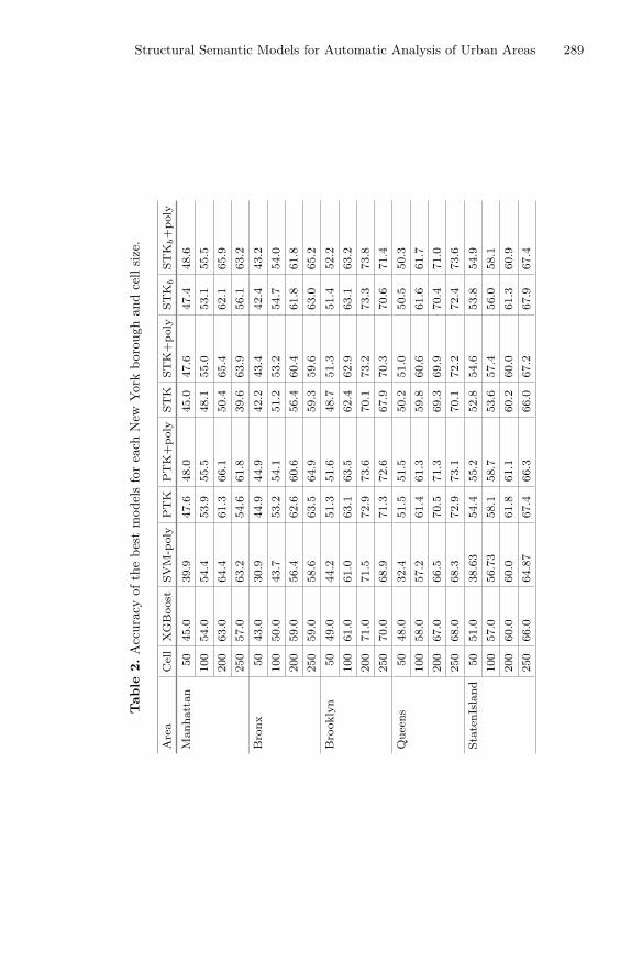
Structural Semantic Models for Automatic Analysis of Urban Areas 289
Table
2.A
ccura
cyofth
ebes
tm
odel
sfo
rea
chN
ewY
ork
boro
ugh
and
cell
size
.
Area
Cell
XGBoost
SVM-poly
PTK
PTK+poly
STK
STK+poly
STK
bSTK
b+poly
Manhattan
50
45.0
39.9
47.6
48.0
45.0
47.6
47.4
48.6
100
54.0
54.4
53.9
55.5
48.1
55.0
53.1
55.5
200
63.0
64.4
61.3
66.1
50.4
65.4
62.1
65.9
250
57.0
63.2
54.6
61.8
39.6
63.9
56.1
63.2
Bronx
50
43.0
30.9
44.9
44.9
42.2
43.4
42.4
43.2
100
50.0
43.7
53.2
54.1
51.2
53.2
54.7
54.0
200
59.0
56.4
62.6
60.6
56.4
60.4
61.8
61.8
250
59.0
58.6
63.5
64.9
59.3
59.6
63.0
65.2
Brooklyn
50
49.0
44.2
51.3
51.6
48.7
51.3
51.4
52.2
100
61.0
61.0
63.1
63.5
62.4
62.9
63.1
63.2
200
71.0
71.5
72.9
73.6
70.1
73.2
73.3
73.8
250
70.0
68.9
71.3
72.6
67.9
70.3
70.6
71.4
Queens
50
48.0
32.4
51.5
51.5
50.2
51.0
50.5
50.3
100
58.0
57.2
61.4
61.3
59.8
60.6
61.6
61.7
200
67.0
66.5
70.5
71.3
69.3
69.9
70.4
71.0
250
68.0
68.3
72.9
73.1
70.1
72.2
72.4
73.6
StatenIsland
50
51.0
38.63
54.4
55.2
52.8
54.6
53.8
54.9
100
57.0
56.73
58.1
58.7
53.6
57.4
56.0
58.1
200
60.0
60.0
61.8
61.1
60.2
60.0
61.3
60.9
250
66.0
64.87
67.4
66.3
66.0
67.2
67.9
67.4
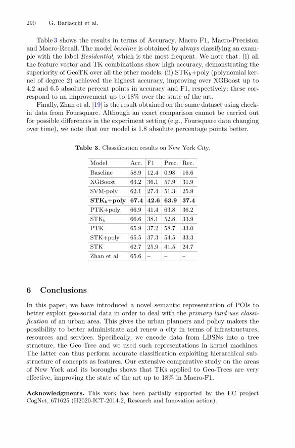
290 G. Barlacchi et al.
Table 3 shows the results in terms of Accuracy, Macro F1, Macro-Precisionand Macro-Recall. The model baseline is obtained by always classifying an exam-ple with the label Residential, which is the most frequent. We note that: (i) allthe feature vector and TK combinations show high accuracy, demonstrating thesuperiority of GeoTK over all the other models. (ii) STKb+poly (polynomial ker-nel of degree 2) achieved the highest accuracy, improving over XGBoost up to4.2 and 6.5 absolute percent points in accuracy and F1, respectively: these cor-respond to an improvement up to 18% over the state of the art.
Finally, Zhan et al. [19] is the result obtained on the same dataset using check-in data from Foursquare. Although an exact comparison cannot be carried outfor possible differences in the experiment setting (e.g., Foursquare data changingover time), we note that our model is 1.8 absolute percentage points better.
Table 3. Classification results on New York City.
Model Acc. F1 Prec. Rec.
Baseline 58.9 12.4 0.98 16.6
XGBoost 63.2 36.1 57.9 31.9
SVM-poly 62.1 27.4 51.3 25.9
STKb+poly 67.4 42.6 63.9 37.4
PTK+poly 66.9 41.4 63.8 36.2
STKb 66.6 38.1 52.8 33.9
PTK 65.9 37.2 58.7 33.0
STK+poly 65.5 37.3 54.5 33.3
STK 62.7 25.9 41.5 24.7
Zhan et al. 65.6 – – –
6 Conclusions
In this paper, we have introduced a novel semantic representation of POIs tobetter exploit geo-social data in order to deal with the primary land use classi-fication of an urban area. This gives the urban planners and policy makers thepossibility to better administrate and renew a city in terms of infrastructures,resources and services. Specifically, we encode data from LBSNs into a treestructure, the Geo-Tree and we used such representations in kernel machines.The latter can thus perform accurate classification exploiting hierarchical sub-structure of concepts as features. Our extensive comparative study on the areasof New York and its boroughs shows that TKs applied to Geo-Trees are veryeffective, improving the state of the art up to 18% in Macro-F1.
Acknowledgments. This work has been partially supported by the EC projectCogNet, 671625 (H2020-ICT-2014-2, Research and Innovation action).

Structural Semantic Models for Automatic Analysis of Urban Areas 291
References
1. Assem, H., Xu, L., Buda, T.S., O’Sullivan, D.: Spatio-temporal clustering approachfor detecting functional regions in cities. In: ICTAI, pp. 370–377. IEEE (2016)
2. Barlacchi, G., De Nadai, M., Larcher, R., Casella, A., Chitic, C., Torrisi, G.,Antonelli, F., Vespignani, A., Pentland, A., Lepri, B.: A multi-source dataset ofurban life in the city of Milan and the Province of Trentino. Sci. Data 2, 150055(2015)
3. Barlacchi, G., Nicosia, M., Moschitti, A.: Sacry: syntax-based automatic crosswordpuzzle resolution system. In: ACL-IJCNLP 2015, p. 79 (2015)
4. Calabrese, F., Di Lorenzo, G., Ratti, C.: Human mobility prediction based onindividual and collective geographical preferences. In: ITSC, pp. 312–317. IEEE(2010)
5. Chen, T., Guestrin, C.: Xgboost: a scalable tree boosting system. In: KDD, pp.785–794. ACM, New York (2016)
6. Collins, M., Duffy, N.: New ranking algorithms for parsing and tagging: kernelsover discrete structures, and the voted perceptron. In: ACL (2002)
7. De Nadai, M., Staiano, J., Larcher, R., Sebe, N., Quercia, D., Lepri, B.: The deathand life of great Italian cities: a mobile phone data perspective. In: Proceedings ofthe 25th International Conference on World Wide Web, pp. 413–423. InternationalWorld Wide Web Conferences Steering Committee (2016)
8. Frias-Martinez, V., Soto, V., Hohwald, H., Frias-Martinez, E.: Characterizingurban landscapes using geolocated tweets. In: SocialCom, pp. 239–248. IEEE(2012)
9. Gartner, T.: A survey of kernels for structured data. ACM SIGKDD Explor. Newsl.5(1), 49–58 (2003)
10. Moschitti, A.: Efficient convolution kernels for dependency and constituent syn-tactic trees. In: Furnkranz, J., Scheffer, T., Spiliopoulou, M. (eds.) ECML 2006.LNCS (LNAI), vol. 4212, pp. 318–329. Springer, Heidelberg (2006). https://doi.org/10.1007/11871842 32
11. Moschitti, A.: Making tree kernels practical for natural language learning. In:EACL, vol. 113, p. 24 (2006)
12. Moschitti, A., Pighin, D., Basili, R.: Tree kernels for semantic role labeling. Com-put. Linguist. 34(2), 193–224 (2008)
13. Noulas, A., Mascolo, C., Frias-Martinez, E.: Exploiting foursquare and cellulardata to infer user activity in urban environments. In: MDM, vol. 1, pp. 167–176.IEEE (2013)
14. Noulas, A., Scellato, S., Mascolo, C., Pontil, M.: Exploiting semantic annotationsfor clustering geographic areas and users in location-based social networks. Soc.Mob. Web 11(2) (2011)
15. Severyn, A., Moschitti, A.: Automatic feature engineering for answer selection andextraction. EMNLP 13, 458–467 (2013)
16. Toole, J.L., Ulm, M., Gonzalez, M.C., Bauer, D.: Inferring land use from mobilephone activity. In: SIGKDD International Workshop on Urban Computing, pp.1–8. ACM (2012)
17. Vishwanathan, S.V.N., Smola, A.J.: Fast kernels for string and tree matching. In:Becker, S., Thrun, S., Obermayer, K. (eds.) NIPS, pp. 569–576. MIT Press (2002)
18. Yuan, J., Zheng, Y., Xie, X.: Discovering regions of different functions in a cityusing human mobility and POIs. In: KDD, pp. 186–194. ACM (2012)
19. Zhan, X., Ukkusuri, S.V., Zhu, F.: Inferring urban land use using large-scale socialmedia check-in data. Netw. Spat. Econ. 14(3–4), 647–667 (2014)
Taking It for a Test Drive: A HybridSpatio-Temporal Model for Wildlife Poaching
Prediction Evaluated Througha Controlled Field Test
Shahrzad Gholami1(B), Benjamin Ford1, Fei Fang2, Andrew Plumptre3,Milind Tambe1, Margaret Driciru4, Fred Wanyama4, Aggrey Rwetsiba4,
Mustapha Nsubaga5, and Joshua Mabonga5
1 University of Southern California, Los Angeles, USA{sgholami,benjamif,tambe}@usc.edu
2 Harvard University, Boston, MA 02138, [email protected]
3 Wildlife Conservation Society, New York City, NY 10460, [email protected]
4 Uganda Wildlife Authority, Kampala, Uganda{margaret.driciru,fred.wanyama,aggrey.rwetsiba}@ugandawildlife.org
5 Wildlife Conservation Society, Kampala, Uganda{mnsubuga,jmabonga}@wcs.org
Abstract. Worldwide, conservation agencies employ rangers to protectconservation areas from poachers. However, agencies lack the manpowerto have rangers effectively patrol these vast areas frequently. While pastwork has modeled poachers’ behavior so as to aid rangers in planningfuture patrols, those models’ predictions were not validated by extensivefield tests. In this paper, we present a hybrid spatio-temporal model thatpredicts poaching threat levels and results from a five-month field test ofour model in Uganda’s Queen Elizabeth Protected Area (QEPA). To ourknowledge, this is the first time that a predictive model has been evalu-ated through such an extensive field test in this domain. We present twomajor contributions. First, our hybrid model consists of two components:(i) an ensemble model which can work with the limited data common tothis domain and (ii) a spatio-temporal model to boost the ensemble’s pre-dictions when sufficient data are available. When evaluated on real-worldhistorical data from QEPA, our hybrid model achieves significantly bet-ter performance than previous approaches with either temporally-awaredynamic Bayesian networks or an ensemble of spatially-aware models.Second, in collaboration with the Wildlife Conservation Society andUganda Wildlife Authority, we present results from a five-month con-trolled experiment where rangers patrolled over 450 sq km across QEPA.We demonstrate that our model successfully predicted (1) where snaringactivity would occur and (2) where it would not occur; in areas wherewe predicted a high rate of snaring activity, rangers found more snares
Shahrzad Gholami and Benjamin Ford are both first authors of this paper.
c© Springer International Publishing AG 2017Y. Altun et al. (Eds.): ECML PKDD 2017, Part III, LNAI 10536, pp. 292–304, 2017.https://doi.org/10.1007/978-3-319-71273-4_24
A Hybrid Spatio-Temporal Model for Wildlife Poaching Prediction 293
and snared animals than in areas of lower predicted activity. These find-ings demonstrate that (1) our model’s predictions are selective, (2) ourmodel’s superior laboratory performance extends to the real world, and(3) these predictive models can aid rangers in focusing their efforts toprevent wildlife poaching and save animals.
Keywords: Predictive models · Ensemble techniquesGraphical models · Field test evaluation · Wildlife protectionWildlife poaching
1 Introduction
Wildlife poaching continues to be a global problem as key species are huntedtoward extinction. For example, the latest African census showed a 30% declinein elephant populations between 2007 and 2014 [1]. Wildlife conservation areashave been established to protect these species from poachers, and these areasare protected by park rangers. These areas are vast, and rangers do not havesufficient resources to patrol everywhere with high intensity and frequency.
At many sites now, rangers patrol and collect data related to snares they con-fiscate, poachers they arrest, and other observations. Given rangers’ resource con-straints, patrol managers could benefit from tools that analyze these data andprovide future poaching predictions. However, this domain presents unique chal-lenges. First, this domain’s real-world data are few, extremely noisy, and incom-plete. To illustrate, one of rangers’ primary patrol goals is to find wire snares, whichare deployed by poachers to catch animals. However, these snares are usually well-hidden (e.g., in dense grass), and thus rangers may not find these snares and (incor-rectly) label an area as not having any snares. Second, poaching activity changesover time, andpredictivemodelsmust account for this temporal component.Third,because poaching happens in the real world, there are mutual spatial and neighbor-hood effects that influence poaching activity. Finally, while field tests are crucial indetermining a model’s efficacy in the world, the difficulties involved in organizingand executing field tests often precludes them.
Previous works in this domain have modeled poaching behavior with real-world data. Based on data from a Queen Elizabeth Protected Area (QEPA)dataset, [6] introduced a two-layered temporal graphical model, CAPTURE,while [4] constructed an ensemble of decision trees, INTERCEPT, that accountedfor spatial relationships. However, these works did not (1) account for bothspatial and temporal components nor (2) validate their models via extensivefield testing.
In this paper, we provide the following contributions. (1) We introduce anew hybrid model that enhances an ensemble’s broad predictive power witha spatio-temporal model’s adaptive capabilities. Because spatio-temporal mod-els require a lot of data, this model works in two stages. First, predictions aremade with an ensemble of decision trees. Second, in areas where there are suf-ficient data, the ensemble’s prediction is boosted via a spatio-temporal model.

294 S. Gholami et al.
(2) In collaboration with the Wildlife Conservation Society and the UgandaWildlife Authority, we designed and deployed a large, controlled experiment toQEPA. Across 27 areas we designated across QEPA, rangers patrolled approxi-mately 452 km over the course of five months; to our knowledge, this is the largestcontrolled experiment and field test of Machine Learning-based predictive mod-els in this domain. In this experiment, we tested our model’s selectiveness: is ourmodel able to differentiate between areas of high and low poaching activity?
In experimental results, (1) we demonstrate our model’s superior perfor-mance over the state-of-the-art [4] and thus the importance of spatio-temporalmodeling. (2) During our field test, rangers found over three times more snaringactivity in areas where we predicted higher poaching activity. When account-ing for differences in ranger coverage, rangers found twelve times the number offindings per kilometer walked in those areas. These results demonstrate that (i)our model is selective in its predictions and (ii) our model’s superior predictiveperformance in the laboratory extends to the real world.
2 Background and Related Work
Spatio-temporal models have been used for prediction tasks in image and videoprocessing. Markov Random Fields (MRF) were used by [11,12] to capturespatio-temporal dependencies in remotely sensed data and moving object detec-tion, respectively.
Critchlow et al. [2] analyzed spatio-temporal patterns in illegal activity inUganda’s Queen Elizabeth Protected Area (QEPA) using Bayesian hierarchicalmodels. With real-world data, they demonstrated the importance of consideringthe spatial and temporal changes that occur in illegal activities. However, inthis work and other similar works with spatio-temporal models [8,9], no stan-dard metrics were provided to evaluate the models’ predictive performance (e.g.,precision, recall). As such, it is impossible to compare our predictive models’ per-formance to theirs. While [3] was a field test of [2]’s work, [8,9] do not conductfield tests to validate their predictions in the real-world.
In the Machine Learning literature, [6] introduced a two-layered temporalBayesian Network predictive model (CAPTURE) that was also evaluated onreal-world data from QEPA. CAPTURE, however, assumes one global set ofparameters for all of QEPA which ignores local differences in poachers’ behavior.Additionally, the first layer, which predicts poaching attacks, relies on the currentyear’s patrolling effort which makes it impossible to predict future attacks (sincepatrols haven’t happened yet). While CAPTURE includes temporal elementsin its model, it does not include spatial components and thus cannot captureneighborhood specific phenomena. In contrast to CAPTURE, [4] presented abehavior model, INTERCEPT, based on an ensemble of decision trees and wasdemonstrated to outperform CAPTURE. While their model accounted for spa-tial correlations, it did not include a temporal component. In contrast to thesepredictive models, our model addresses both spatial and temporal components.
It is vital to validate predictive models in the real world, and both [3,4] haveconducted field tests in QEPA. [4] conducted a one month field test in QEPA

A Hybrid Spatio-Temporal Model for Wildlife Poaching Prediction 295
and demonstrated promising results for predictive analytics in this domain.Unlike the field test we conducted, however, that was a preliminary field testand was not a controlled experiment. On the other hand, [3] conducted a con-trolled experiment where their goal, by selecting three areas for rangers to patrol,was to maximize the number of observations sighted per kilometer walked bythe rangers. Their test successfully demonstrated a significant increase in illegalactivity detection at two of the areas, but they did not provide comparable eval-uation metrics for their predictive model. Also, our field test was much larger inscale, involving 27 patrol posts compared to their 9 posts.
3 Wildlife Crime Dataset: Features and Challenges
This study’s wildlife crime dataset is from Uganda’s Queen Elizabeth ProtectedArea (QEPA), an area containing a wildlife conservation park and two wildlifereserves, which spans about 2,520 km2. There are 37 patrol posts situated acrossQEPA from which Uganda Wildlife Authority (UWA) rangers conduct patrolsto apprehend poachers, remove any snares or traps, monitor wildlife, and recordsigns of illegal activity. Along with the amount of patrolling effort in each area,the dataset contains 14 years (2003–2016) of the type, location, and date ofwildlife crime activities.
Rangers lack the manpower to patrol everywhere all the time, and thus illegalactivity may be undetected in unpatrolled areas. Patrolling is an imperfect pro-cess, and there is considerable uncertainty in the dataset’s negative data points(i.e., areas being labeled as having no illegal activity); rangers may patrol anarea and label it as having no snares when, in fact, a snare was well-hiddenand undetected. These factors contribute to the dataset’s already large classimbalance; there are many more negative data points than there are positivepoints (crime detected). It is thus necessary to consider models that estimatehidden variables (e.g., whether an area has been attacked) and also to evaluatepredictive models with metrics that account for this uncertainty, such as thosein the Positive and Unlabeled Learning (PU Learning) literature [5]. We divideQEPA into 1 km2 grid cells (a total of 2,522 cells), and we refer to these cellsas targets. Each target is associated with several static geospatial features suchas terrain (e.g., slope), distance values (e.g., distance to border), and animaldensity. Each target is also associated with dynamic features such as how oftenan area has been patrolled (i.e., coverage) and observed illegal activities (e.g.,snares) (Fig. 1).
4 Models and Algorithms
4.1 Prediction by Graphical Models
Markov Random Field (MRF). To predict poaching activity, each target,at time step t ∈ {t1, ..., tm}, is represented by coordinates i and j within theboundary of QEPA. In Fig. 2(a), we demonstrate a three-dimensional network

296 S. Gholami et al.
(a) Snare (b) QEPA grid
Fig. 1. Photo credit: UWA ranger
(a) Spatio-temporal model (b) Geo-Clusters
Fig. 2. Geo-clusters and graphical model
for spatio-temporal modeling of poaching events over all targets. Connectionsbetween nodes represent the mutual spatial influence of neighboring targets andalso the temporal dependence between recurring poaching incidents at a target.ati,j represents poaching incidents at time step t and target i, j. Mutual spatialinfluences are modeled through first-order neighbors (i.e., ati,j connects to ati±1,j ,ati,j±1 and at−1
i,j ) and second-order neighbors (i.e., ati,j connects to ati±1,j±1); forsimplicity, the latter is not shown on the model’s lattice. Each random variabletakes a value in its state space, in this paper, L = {0, 1}.
To avoid index overload, henceforth, nodes are indexed by serial numbers,S = {1, 2, ..., N} when we refer to the three-dimensional network. We intro-duce two random fields, indexed by S, with their configurations: A = {a =(a1, ..., aN )|ai ∈ L, i ∈ S}, which indicates an actual poaching attack occurredat targets over the period of study, and O = {o = (o1, ..., oN )|oi ∈ L, i ∈ S}indicates a detected poaching attack at targets over the period of study. Dueto the imperfect detection of poaching activities, the former represents the hid-den variables, and the latter is the known observed data collected by rangers,shown by the gray-filled nodes in Fig. 2(a). Targets are related to one anothervia a neighborhood system, Nn, which is the set of nodes neighboring n andn �∈ Nn. This neighborhood system considers all spatial and temporal neigh-bors. We define neighborhood attackability as the fraction of neighbors that themodel predicts to be attacked: uNn
=∑
n∈Nnan/|Nn|.
The probability, P (ai|uNn,α), of a poaching incident at each target n at
time step t is represented in Eq. 1, where α is a vector of parameters weightingthe most important variables that influence poaching; Z represents the vectorof time-invariant ecological covariates associated with each target (e.g., animaldensity, slope, forest cover, net primary productivity, distance from patrol post,town and rivers [2,7]). The model’s temporal dimension is reflected through notonly the backward dependence of each an, which influences the computation ofuNn
, but also in the past patrol coverage at target n, denoted by ct−1n , which
models the delayed deterrence effect of patrolling efforts.
p(an = 1|uNn,α) =
e−α [Z ,uNn ,ct−1n ,1]ᵀ
1 + e−α [Z ,uNn ,ct−1n ,1]ᵀ
(1)
Given an, on follows a conditional probability distribution proposed in Eq. 2,which represents the probability of rangers detecting a poaching attack at targetn.

A Hybrid Spatio-Temporal Model for Wildlife Poaching Prediction 297
The first column of the matrix denotes the probability of not detecting or detectingattacks if an attack has not happened, which is constrained to 1 or 0 respectively.In other words, it is impossible to detect an attack when an attack has not hap-pened. The second column of the matrix represents the probability of not detect-ing or detecting attacks in the form of a logistic function if an attack has happened.Since it is less rational for poachers to place snares close to patrol posts and moreconvenient for rangers to detect poaching signs near the patrol posts, we assumeddpn (distance from patrol post) and ctn (patrol coverage devoted to target n at timet) are the major variables influencing rangers’ detection capabilities. Detectabilityat each target is represented in Eq. 2, where β is a vector of parameters that weightthese variables.
p(on|an) =
[p(on = 0|an = 0) p(on = 0|an = 1,β)
p(on = 1|an = 0) p(on = 1|an = 1,β)
]=
⎡⎢⎢⎣
1,1
1 + e−β [dpn,ctn,1]ᵀ
0,e−β [dpn,ctn,1]ᵀ
1 + e−β [dpn,ctn,1]ᵀ
⎤⎥⎥⎦ (2)
We assume that (o,a) is pairwise independent, meaning p(o,a) =∏n∈S p(on, an).
EM Algorithm to Infer on MRF. We use the Expectation-Maximization(EM) algorithm to estimate the MRF model’s parameters θ = {α,β}. For com-pleteness, we provide details about how we apply the EM algorithm to ourmodel. Given a joint distribution p(o,a|θ) over observed variables o and hid-den variables a, governed by parameters θ, EM aims to maximize the likelihoodfunction p(o|θ) with respect to θ. To start the algorithm, an initial setting forthe parameters θold is chosen. At E-step, p(a|o,θold) is evaluated, particularly,for each node in MRF model:
p(an|on,θold) =p(on|an,βold).p(an|uold
Nn,αold)
p(on)(3)
M-step calculates θnew, according to the expectation of the complete log likeli-hood, log p(o,a|θ), given in Eq. 4.
θnew = arg maxθ
∑
an∈Lp(a|o,θold). log p(o,a|θ) (4)
To facilitate calculation of the log of the joint probability distribution,log p(o,a|θ), we introduce an approximation that makes use of uold
Nn, represented
in Eq. 5.
log p(o,a|θ) =∑
n∈S
∑
an∈Llog p(on|an,β) + log p(an|uold
Nn,α) (5)
Then, if convergence of the log likelihood is not satisfied, θold ← θnew, andrepeat.

298 S. Gholami et al.
Dataset Preparation for MRF. To split the data into training and testsets, we divided the real-world dataset into year-long time steps. We trained themodel’s parameters θ = {α,β} on historical data sampled through time steps(t1, ..., tm) for all targets within the boundary. These parameters were used topredict poaching activity at time step tm+1, which represents the test set forevaluation purposes. The trade-off between adding years’ data (performance)vs. computational costs led us to use three years (m = 3). The model was thustrained over targets that were patrolled throughout the training time period(t1, t2, t3). We examined three training sets: 2011–2013, 2012–2014, and 2013–2015 for which the test sets are from 2014, 2015, and 2016, respectively.
Capturing temporal trends requires a sufficient amount of data to be collectedregularly across time steps for each target. Due to the large amount of missinginspections and uncertainty in the collected data, this model focuses on learningpoaching activity only over regions that have been continually monitored in thepast, according to Definition 1. We denote this subset of targets as Sc.
Definition 1. Continually vs. occasionally monitoring: A target i, j iscontinually monitored if all elements of the coverage sequence are positive; ctki,j >0,∀k = 1, ...,m where m is the number of time steps. Otherwise, it is occasionallymonitored.
Experiments with MRF were conducted in various ways on each data set.We refer to (a) a global model with spatial effects as GLB-S, which consistsof a single set of parameters θ for the whole QEPA, and (b) a global modelwithout spatial effects (i.e., the parameter that corresponds to uNn
is set to0) as GLB. The spatio-temporal model is designed to account for temporaland spatial trends in poaching activities. However, since learning those trendsand capturing spatial effects are impacted by the variance in local poachers’behaviors, we also examined (c) a geo-clustered model which consists of multiplesets of local parameters throughout QEPA with spatial effects, referred to asGCL-S, and also (d) a geo-clustered model without spatial effects (i.e., theparameter that corresponds to uNn
is set to 0) referred to as GCL.Figure 2(b) shows the geo-clusters generated by Gaussian Mixture Models
(GMM), which classifies the targets based on the geo-spatial features, Z, alongwith the targets’ coordinates, (xi,j , yi,j), into 22 clusters. The number of geo-clusters, 22, are intended to be close to the number of patrol posts in QEPAsuch that each cluster contains one or two nearby patrol posts. With that beingconsidered, not only are local poachers’ behaviors described by a distinct set ofparameters, but also the data collection conditions, over the targets within eachcluster, are maintained to be nearly uniform.
4.2 Prediction by Ensemble Models
A Bagging ensemble model or Bootstrap aggregation technique, called Bag-ging, is a type of ensemble learning which bags some weak learners, such asdecision trees, on a dataset by generating many bootstrap duplicates of the

A Hybrid Spatio-Temporal Model for Wildlife Poaching Prediction 299
dataset and learning decision trees on them. Each of the bootstrap duplicatesare obtained by randomly choosing M observations out of M with replacement,where M denotes the training dataset size. Finally, the predicted response of theensemble is computed by taking an average over predictions from its individualdecision trees. To learn a Bagging ensemble, we used the fitensemble functionof MATLAB 2017a. Dataset preparation for the Bagging ensemble model isdesigned to find the targets that are liable to be attacked [4]. A target is assumedto be attackable if it has ever been attacked; if any observations occurred in theentire training period for a given target, that target is labeled as attackable. Forthis model, the best training period contained 5 years of data.
4.3 Hybrid of MRF and Bagging Ensemble
Since the amount and regularity of data collected by rangers varies across regionsof QEPA, predictive models perform differently in different regions. As such, wepropose using different models to predict over them; first, we used a Baggingensemble model, and then improved the predictions in some regions using thespatio-temporal model. For global models, we used MRF for all continually mon-itored targets. However, for geo-clustered models, for targets in the continuallymonitored subset, Sq
c , (where temporally-aware models can be used practically),the MRF model’s performance varied widely across geo-clusters according toour experiments. q indicates clusters and 1 ≤ q ≤ 22. Thus, for each q, if theaverage Catch Per Unit Effort (CPUE), outlined by Definition 2, is relativelylarge, we use the MRF model for Sq
c . In Conservation Biology, CPUE is an indi-rect measure of poaching activity abundance. A larger average CPUE for eachcluster corresponds to more frequent poaching activity and thus more data forthat cluster. Consequently, using more complex spatio-temporal models in thoseclusters becomes more reasonable.
Definition 2. Average CPUE is∑
n∈Sqcon/
∑n∈Sq
cctn in cluster q.
To compute CPUE, effort corresponds to the amount of coverage (i.e., 1 unit =1 km walked) in a given target, and catch corresponds to the number of observa-tions. Hence, for 1 ≤ q ≤ 22, we will boost selectively according to the averageCPUE value; some clusters may not be boosted by MRF, and we would only useBagging ensemble model for making predictions on them. Experiments on his-torical data show that selecting 15% of the geo-clusters with the highest averageCPUE results in the best performance for the entire hybrid model (discussed inthe Evaluation Section).
5 Evaluations and Discussions
5.1 Evaluation Metrics
The imperfect detection of poaching activities in wildlife conservation areas leadsto uncertainty in the negative class labels of data samples [4]. It is thus vital
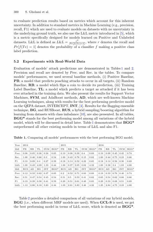
300 S. Gholami et al.
to evaluate prediction results based on metrics which account for this inherentuncertainty. In addition to standard metrics in Machine Learning (e.g., precision,recall, F1) which are used to evaluate models on datasets with no uncertainty inthe underlying ground truth, we also use the L&L metric introduced in [5], whichis a metric specifically designed for models learned on Positive and Unlabeleddatasets. L&L is defined as L&L = r2
Pr[f(Te)=1] , where r denotes the recall andPr[f(Te) = 1] denotes the probability of a classifier f making a positive classlabel prediction.
5.2 Experiments with Real-World Data
Evaluation of models’ attack predictions are demonstrated in Tables 1 and 2.Precision and recall are denoted by Prec. and Rec. in the tables. To comparemodels’ performances, we used several baseline methods, (i) Positive Baseline,PB; a model that predicts poaching attacks to occur in all targets, (ii) RandomBaseline, RB; a model which flips a coin to decide its prediction, (iii) TrainingLabel Baseline, TL; a model which predicts a target as attacked if it has beenever attacked in the training data. We also present the results for Support VectorMachines, SVM, and AdaBoost methods, AD, which are well-known MachineLearning techniques, along with results for the best performing predictive modelon the QEPA dataset, INTERCEPT, INT, [4]. Results for the Bagging ensembletechnique, BG, and RUSBoost, RUS, a hybrid sampling/boosting algorithm forlearning from datasets with class imbalance [10], are also presented. In all tables,BGG* stands for the best performing model among all variations of the hybridmodel, which will be discussed in detail later. Table 1 demonstrates that BGG*outperformed all other existing models in terms of L&L and also F1.
Table 1. Comparing all models’ performances with the best performing BGG model.
Year 2014 2015 2016
Mdl PB RB TL SVM BGG* PB RB TL SVM BGG* PB RB TL SVM BGG*
Prec. 0.06 0.05 0.26 0.24 0.65 0.10 0.08 0.39 0.4 0.69 0.10 0.09 0.45 0.45 0.74
Rec. 1.00 0.46 0.86 0.3 0.54 1.00 0.43 0.78 0.15 0.62 1.00 0.44 0.75 0.23 0.66
F1 0.10 0.09 0.4 0.27 0.59 0.18 0.14 0.52 0.22 0.65 0.18 0.14 0.56 0.30 0.69
L&L 1.00 0.43 4.09 1.33 6.44 1.00 0.37 3.05 0.62 4.32 1.00 0.38 3.4 1.03 4.88
Mdl RUS AD BG INT BGG* RUS AD BG INT BGG* RUS AD BG INT BGG*
Prec. 0.12 0.33 0.62 0.37 0.65 0.2 0.52 0.71 0.63 0.69 0.19 0.53 0.76 0.40 0.74
Rec. 0.51 0.47 0.54 0.45 0.54 0.51 0.5 0.53 0.41 0.62 0.65 0.54 0.62 0.66 0.66
F1 0.19 0.39 0.58 0.41 0.59 0.29 0.51 0.61 0.49 0.65 0.29 0.53 0.68 0.51 0.69
L&L 1.12 2.86 6.18 5.83 6.44 1.03 2.61 3.83 3.46 4.32 1.25 2.84 4.75 2.23 4.88
Table 2 provides a detailed comparison of all variations of our hybrid models,BGG (i.e., when different MRF models are used). When GCL-S is used, we getthe best performing model in terms of L&L score, which is denoted as BGG*.
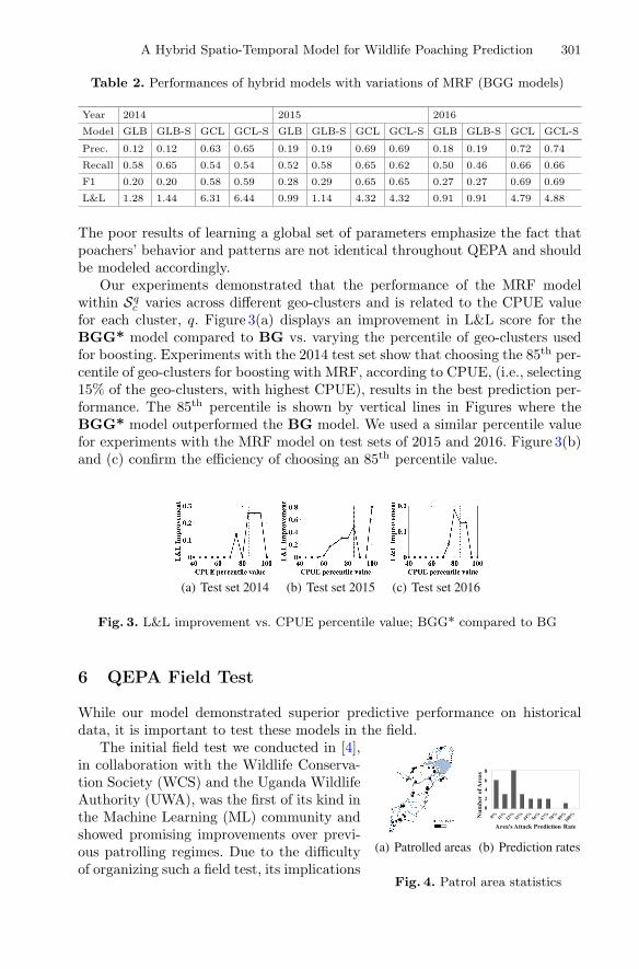
A Hybrid Spatio-Temporal Model for Wildlife Poaching Prediction 301
Table 2. Performances of hybrid models with variations of MRF (BGG models)
Year 2014 2015 2016
Model GLB GLB-S GCL GCL-S GLB GLB-S GCL GCL-S GLB GLB-S GCL GCL-S
Prec. 0.12 0.12 0.63 0.65 0.19 0.19 0.69 0.69 0.18 0.19 0.72 0.74
Recall 0.58 0.65 0.54 0.54 0.52 0.58 0.65 0.62 0.50 0.46 0.66 0.66
F1 0.20 0.20 0.58 0.59 0.28 0.29 0.65 0.65 0.27 0.27 0.69 0.69
L&L 1.28 1.44 6.31 6.44 0.99 1.14 4.32 4.32 0.91 0.91 4.79 4.88
The poor results of learning a global set of parameters emphasize the fact thatpoachers’ behavior and patterns are not identical throughout QEPA and shouldbe modeled accordingly.
Our experiments demonstrated that the performance of the MRF modelwithin Sq
c varies across different geo-clusters and is related to the CPUE valuefor each cluster, q. Figure 3(a) displays an improvement in L&L score for theBGG* model compared to BG vs. varying the percentile of geo-clusters usedfor boosting. Experiments with the 2014 test set show that choosing the 85th per-centile of geo-clusters for boosting with MRF, according to CPUE, (i.e., selecting15% of the geo-clusters, with highest CPUE), results in the best prediction per-formance. The 85th percentile is shown by vertical lines in Figures where theBGG* model outperformed the BG model. We used a similar percentile valuefor experiments with the MRF model on test sets of 2015 and 2016. Figure 3(b)and (c) confirm the efficiency of choosing an 85th percentile value.
(a) Test set 2014 (b) Test set 2015 (c) Test set 2016
Fig. 3. L&L improvement vs. CPUE percentile value; BGG* compared to BG
6 QEPA Field Test
While our model demonstrated superior predictive performance on historicaldata, it is important to test these models in the field.
(a) Patrolled areas
0
2
4
6
8
Num
ber
of A
reas
Area's Attack Prediction Rate
(b) Prediction rates
Fig. 4. Patrol area statistics
The initial field test we conducted in [4],in collaboration with the Wildlife Conserva-tion Society (WCS) and the Uganda WildlifeAuthority (UWA), was the first of its kind inthe Machine Learning (ML) community andshowed promising improvements over previ-ous patrolling regimes. Due to the difficultyof organizing such a field test, its implications

302 S. Gholami et al.
were limited: only two 9-km2 areas (18 km2) of QEPA were patrolled by rangersover a month. Because of its success, however, WCS and UWA graciously agreedto a larger scale, controlled experiment: also in 9 km2 areas, but rangers patrolled27 of these areas (243 km2, spread across QEPA) over five months; this is thelargest to-date field test of ML-based predictive models in this domain. We showthe areas in Fig. 4(a). Note that rangers patrolled these areas in addition to otherareas of QEPA as part of their normal duties.
This experiment’s goal was to determine the selectiveness of our model’ssnare attack predictions: does our model correctly predict both where there areand are not snare attacks? We define attack prediction rate as the proportion oftargets (a 1 km by 1 km cell) in a patrol area (3 by 3 cells) that are predictedto be attacked. We considered two experiment groups that corresponded to ourmodel’s attack prediction rates from November 2016 to March 2017: High (group1) and Low (group 2). Areas that had an attack prediction rate of 50% or greaterwere considered to be in a high area (group 1); areas with less than a 50% ratewere in group 2. For example, if the model predicted five out of nine targetsto be attacked in an area, that area was in group 1. Due to the importance ofQEPA for elephant conservation, we do not show which areas belong to whichexperiment group in Fig. 4(a) so that we do not provide data to ivory poachers.
To start, we exhaustively generated all patrol areas such that (1) each patrolarea was 3 × 3 km2, (2) no point in the patrol area was more than 5 km away fromthe nearest ranger patrol post, and (3) no patrol area was patrolled too frequentlyor infrequently in past years (to ensure that the training data associated with allareas was of similar quality); in all, 544 areas were generated across QEPA. Then,using the model’s attack predictions, each area was assigned to an experimentgroup. Because we were not able to test all 544 areas, we selected a subset suchthat no two areas overlapped with each other and no more than two areas wereselected for each patrol post (due to manpower constraints). In total, 5 areas ingroup 1 and 22 areas in group 2 were chosen. Note that this composition arosedue to the preponderance of group 2 areas (see Table 3). We provide a breakdownof the areas’ exact attack prediction rates in Fig. 4(b); areas with rates below56% (5/9) were in group 2, and for example, there were 8 areas in group 2 with arate of 22% (2/9). Finally, when we provided patrols to the rangers, experimentgroup memberships were hidden to prevent effects where knowledge of predictedpoaching activity would influence their patrolling patterns and detection rates.
Table 3. Patrol area group memberships
Experiment group Exhaustive patrol area groups Final patrol area groups
High (1) 50 (9%) 5 (19%)
Low (2) 494 (91%) 22 (81%)

A Hybrid Spatio-Temporal Model for Wildlife Poaching Prediction 303
6.1 Field Test Results and Discussion
The field test data we received was in the same format as the historical data.However, because rangers needed to physically walk to these patrol areas, wereceived additional data that we have omitted from this analysis; observationsmade outside of a designated patrol area were not counted. Because we onlypredicted where snaring activity would occur, we have also omitted other obser-vation types made during the experiment (e.g., illegal cattle grazing). We presentresults from this five-month field test in Table 4. To provide additional contextfor these results, we also computed QEPA’s park-wide historical CPUE (fromNovember 2015 to March 2016): 0.04.
Table 4. Field test results: observations
Experiment group Observation count (%) Mean count (std) Effort (%) CPUE
High (1) 15 (79%) 3 (5.20) 129.54 (29%) 0.12
Low (2) 4 (21%) 0.18 (0.50) 322.33 (71%) 0.01
Areas with a high attack prediction rate (group 1) had significantly moresnare sightings than areas with low attack prediction rates (15 vs. 4). This isdespite there being far fewer group 1 areas than group 2 areas (5 vs. 22); onaverage, group 1 areas had 3 snare observations whereas group 2 areas had0.18 observations. It is worth noting the large standard deviation for the meanobservation counts; the standard deviation of 5.2, for the mean of 3, signifiesthat not all areas had snare observations. Indeed, two out of five areas in group1 had snare observations. However, this also applies to group 2’s areas: only 3out of 22 areas had snare observations.
We present Catch per Unit Effort (CPUE) results in Table 4. When account-ing for differences in areas’ effort, group 1 areas had a CPUE that was over tentimes that of group 2 areas. Moreover, when compared to QEPA’s park-widehistorical CPUE of 0.04, it is clear that our model successfully differentiatedbetween areas of high and low snaring activity. The results of this large-scalefield test, the first of its kind for ML models in this domain, demonstrated thatour model’s superior predictive performance in the laboratory extends to thereal world.
7 Conclusion
In this paper, we presented a hybrid spatio-temporal model to predict wildlifepoaching threat levels. Additionally, we validated our model via an extensivefive-month field test in Queen Elizabeth Protected Area (QEPA) where rangerspatrolled over 450 km2 across QEPA—the largest field-test to-date of MachineLearning-based models in this domain. On real-world historical data from QEPA,our hybrid model achieves significantly better performance than prior work. Onthe data collected from our field test, we demonstrated that our model success-fully differentiated between areas of high and low snaring activity. These findings

304 S. Gholami et al.
demonstrated that our model’s predictions are selective and also that its supe-rior laboratory performance extends to the real world. Based on these promisingresults, future work will focus on deploying these models as part of a softwarepackage to UWA to aid in planning future anti-poaching patrols.
Acknowledgments. This research was supported by MURI grant W911NF-11-1-0332, NSF grant with Cornell University 72954-10598 and partially supported by Har-vard Center for Research on Computation and Society fellowship. We are grateful to theWildlife Conservation Society and the Uganda Wildlife Authority for supporting datacollection in QEPA. We also thank Donnabell Dmello for her help in data processing.
References
1. Great Elephant Census: The great elephant census—a Paul G. Allen project. PressRelease, August 2016
2. Critchlow, R., Plumptre, A., Driciru, M., Rwetsiba, A., Stokes, E., Tumwesigye,C., Wanyama, F., Beale, C.: Spatiotemporal trends of illegal activities from ranger-collected data in a Ugandan National Park. Conserv. Biol. 29(5), 1458–1470 (2015)
3. Critchlow, R., Plumptre, A.J., Alidria, B., Nsubuga, M., Driciru, M., Rwetsiba, A.,Wanyama, F., Beale, C.M.: Improving law-enforcement effectiveness and efficiencyin protected areas using ranger-collected monitoring data. Conserv. Lett. 10(5),572–580 (2017). Wiley Online Library
4. Kar, D., Ford, B., Gholami, S., Fang, F., Plumptre, A., Tambe, M., Driciru, M.,Wanyama, F., Rwetsiba, A., Nsubaga, M., et al.: Cloudy with a chance of poach-ing: adversary behavior modeling and forecasting with real-world poaching data.In: Proceedings of the 16th Conference on Autonomous Agents and MultiAgentSystems, pp. 159–167 (2017)
5. Lee, W.S., Liu, B.: Learning with positive and unlabeled examples using weightedlogistic regression. In: ICML, vol. 3 (2003)
6. Nguyen, T.H., Sinha, A., Gholami, S., Plumptre, A., Joppa, L., Tambe, M., Driciru,M., Wanyama, F., Rwetsiba, A., Critchlow, R., et al.: CAPTURE: a new predictiveanti-poaching tool for wildlife protection. In: AAMAS, pp. 767–775 (2016)
7. O’Kelly, H.J.: Monitoring Conservation Threats, Interventions, and Impacts onWildlife in a Cambodian Tropical Forest, p. 149. Imperial College, London (2013)
8. Rashidi, P., Wang, T., Skidmore, A., Mehdipoor, H., Darvishzadeh, R., Ngene, S.,Vrieling, A., Toxopeus, A.G.: Elephant poaching risk assessed using spatial andnon-spatial Bayesian models. Ecol. Model. 338, 60–68 (2016)
9. Rashidi, P., Wang, T., Skidmore, A., Vrieling, A., Darvishzadeh, R., Toxopeus, B.,Ngene, S., Omondi, P.: Spatial and spatiotemporal clustering methods for detectingelephant poaching hotspots. Ecol. Model. 297, 180–186 (2015)
10. Seiffert, C., Khoshgoftaar, T.M., Van Hulse, J., Napolitano, A.: Rusboost: a hybridapproach to alleviating class imbalance. IEEE SMC-A Syst. Hum. 40(1), 185–197(2010)
11. Solberg, A.H.S., Taxt, T., Jain, A.K.: A Markov random field model for classifica-tion of multisource satellite imagery. IEEE TGRS 34(1), 100–113 (1996)
12. Yin, Z., Collins, R.: Belief propagation in a 3d spatio-temporal MRF for movingobject detection. In: IEEE CVPR, pp. 1–8. IEEE (2007)
Unsupervised Signature Extractionfrom Forensic Logs
Stefan Thaler1(B), Vlado Menkovski1, and Milan Petkovic1,2
1 Technical University of Eindhoven,Den Dolech 12, 5600 MB Eindhoven, Netherlands
{s.m.thaler,v.menkovski}@tue.nl2 Philips Research Laboratories,
High Tech Campus 34, Eindhoven, [email protected]
Abstract. Signature extraction is a key part of forensic log analysis. Itinvolves recognizing patterns in log lines such that log lines that origi-nated from the same line of code are grouped together. A log signatureconsists of immutable parts and mutable parts. The immutable partsdefine the signature, and the mutable parts are typically variable para-meter values. In practice, the number of log lines and signatures can bequite large, and the task of detecting and aligning immutable parts ofthe logs to extract the signatures becomes a significant challenge. Wepropose a novel method based on a neural language model that out-performs the current state-of-the-art on signature extraction. We use anRNN auto-encoder to create an embedding of the log lines. Log linesembedded in such a way can be clustered to extract the signatures in anunsupervised manner.
Keywords: Information forensic · RNN auto-encoderNeural language model · Log clustering · Signature extraction
1 Introduction
An important step of an information forensic investigation is log analysis. Logscontain valuable information for reconstructing incidents that have happenedon a computer system. In this context, a log line is a sequence of tokens thatgive information about the state of a process that created this log line. Thetokens of each log lines are partially natural language and partially structureddata. Tokens may be words, numbers, variables or punctuation characters suchas brackets, colons or dots.
Log signatures are the print statements that produce the log lines. Log sig-natures have fixed parts and may have variable parts. Fixed parts consist ofa sequence of tokens of arbitrary length that uniquely identify signatures. Thevariable parts may also be of arbitrary length and variable parts in log lines thatoriginate from the same signature differ.c© Springer International Publishing AG 2017Y. Altun et al. (Eds.): ECML PKDD 2017, Part III, LNAI 10536, pp. 305–316, 2017.https://doi.org/10.1007/978-3-319-71273-4_25

306 S. Thaler et al.
The goal of a forensic investigator is to uncover a sequence of events froma forensic log that reveal a security incident. The sequence of events describesthe actions that the users of this computer system took. Traces of these actionsare typically stored in logs. Similar events may have different log lines associatedwith them because the variable part reports the state of the system at that time,which makes finding such events difficult. Knowing the log signatures of a logenable a forensic investigator to group together log lines that belong to the sameevent, even though the log lines differ. Finding such signatures is challengingbecause of the unknown number of signatures and the unknown number andposition of fixed parts. Signature extraction is the process of finding a set of logsignatures given a set of log lines.
State-of-the-art approaches identify log signatures based on the position andfrequency of tokens [1,12,23]. These approaches typically assume that frequentwords define the fixed parts of the signature. This assumption holds if the ratioof log lines per signature in the analyzed log is high. This can be the case formany application logs where the tokens of fixed signature parts are repeated witha high frequency. However, in information forensics, logs commonly have manysignatures but few log lines per signature. In this case, the number of occurrenceof tokens of variable parts may be higher than fixed tokens, which can cause aconfusion of which tokens are fixed and which ones are variable. Confusing fixedtokens with variable ones leads to signatures that match too few log lines, andmixing variable tokens with fixed ones will result into signatures that will matchtoo few log lines.
To address the challenge of signature extraction from forensic logs, we pro-pose to use a method that takes contextual information about the tokens intoaccount. Our approach is inspired by recent advances in the NLP domain, wheresequence-to-sequence models have been successfully used to capture natural lan-guage [3,9].
Signature B
LSTM decoder
LSTM encoder
Signature AEmbedded Space
h
userSession opened root ( uid = 0 )
userSession opened root ( uid = 0 )Target:reversedlog line
Input:log line
Fig. 1. We first embed forensic log lines using an RNN auto-encoder. We then clusterthe embedded log lines and assign them to a signature.
Typically, sequence-to-sequence models consist of two recurrent neural net-works (RNNs), an encoder network and a decoder network. The encoder networklearns to represent an input sequence, and the decoder learns to construct the
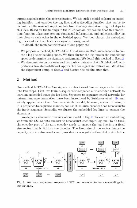
Unsupervised Signature Extraction from Forensic Logs 307
output sequence from this representation. We use such a model to learn an encod-ing function that encodes the log line, and a decoding function that learns toreconstruct the reversed input log line from this representation. Figure 1 depictsthis idea. Based on the findings in the NLP domain, we assume that this embed-ding function takes into account contextual information, and embeds similar loglines close to each other in the embedded space. We then cluster the embeddedlog lines and use the clusters as signature assignment.
In detail, the main contributions of our paper are:
– We propose a method, LSTM-AE+C, that uses an RNN auto-encoder to cre-ate a log line embedding space. We then cluster the log lines in the embeddingspace to determine the signature assignment. We detail this method in Sect. 2.
– We demonstrate on our own and two public datasets that LSTM-AE+C out-performs two state-of-the-art approaches for signature extraction. We detailthe experiment setup in Sect. 3 and discuss the results after that.
2 Method
Our method LSTM-AE+C for signature extraction of forensic logs can be dividedinto two steps. First, we train a sequence-to-sequence auto-encoder network tolearn an embedded space for log lines. Sequence-to-sequence neural networks fornatural language translation have been introduced by Sutskever et al. [19] andwidely applied since then. We use a similar model, however, instead of using itin a sequence-to-sequence manner, we use it as auto-encoder that reconstructsthe input sequence. Secondly, we cluster the embedded log lines to extract thesignatures.
We depict a schematic overview of our model in Fig. 2. To learn an embeddingwe train the LSTM auto-encoder to reconstruct each input log line. To do that,the encoder part of the auto-encoder needs to encode the log line into a fixedsize vector that is fed into the decoder. The fixed size of the vector limits thecapacity of the auto-encoder and provides for a regularization that restricts the
Fig. 2. We use a sequence-to-sequence LSTM auto-encoder to learn embeddings forour log lines.

308 S. Thaler et al.
auto-encoder from learning an identity function. We use that representation asembedding for the log lines. In the remaining section we will first detail thecomponents of our model and their relationships to each other, then detail thelearning objective and finally describe how we extract signatures.
2.1 Model
The input to our model is log lines. We treat log lines as a sequence of tokensof length n, where a token can be a word, variable part or delimiter. The set ofunique tokens is our input vocabulary, where each token in the vocabulary getsa unique id.
Since the number of such tokens in a log can be potentially very large, welearn a dense representation for the tokens of our log lines. To get these denserepresentations, we use a token embedding matrix E(v×u), where v is the uniquenumber of tokens that we have in our token vocabulary and u is the numberof hidden units of the encoder network. The index of each row of E is also theposition of v in the vocabulary. We denote an in E embedded token as w.
Next, want to learn the log line embedding. To do so, we learn an encoderfunction ENC using an LSTM [7], which is a variant of a recurrent neural net-work. We chose an LSTM for both the encoder and decoder, because it addressesthe vanishing gradient problem. he(t) is the hidden encoder state at time step t,and y
(t)e is the encoder output at time step t. w
(t)e is the embedded input word
for time step t. We use the encoding state and and input word at each timestep to calculate the next state and the next output. We discard all output s ofthe encoder. We use the final hidden state h
(n)e to embed our log lines. h
(n)e also
serves as initial hidden state for our decoder network.
(y(t)e , h(t+1)
e ) = ENC(w(t)e , h(t)
e )
Our decoder function DEC is trained to learn to reconstruct the reversesequence S′ given the last hidden state h
(n)e of our encoding network. The struc-
ture of the network is identical to the encoder, except we feed the network thereverse sequence of embedded tokens as input.
(y(t)d , h
(t+1)d ) = DEC(w(t)
d , h(t)d )
From the decoder outputs y(t)d we predict the reverse sequence of tokens S′.
Calculating a softmax function for a large token vocabulary is computationallyvery expensive because the softmax function is calculated as the sum over allpotential classes. Therefore, we predict the output tokens of our decoder sequenceusing sampled softmax [8]. Sampled softmax is a candidate training method thatapproximates the desired softmax function by solving a task that does not requirepredicting the correct token from all token. Instead, the task sampled softmaxsolves is to identify the correct token from a randomly drawn sample of tokens.

Unsupervised Signature Extraction from Forensic Logs 309
2.2 Objective
To embed our log lines in an embedded space, the model needs to maximize theprobability of predicting a reversed sequence of tokens S′ given a sequence oftokens S. In other words, we want to train the encoding network to learn anembedding that contains enough information for the decoder to reconstruct it.However, as an effect of the regularization, we expect the model to use the struc-ture to use the structure of the log lines to create a more efficient representation,that in turn allows us to extract the signatures.
θ∗ = arg maxθ
∑
(S,S′)
log p(S′|S; θ)
θ are the parameters of our model, S represents a log line, and S′ representsa reversed log line.
S is a sequence of tokens of arbitrary length. To model the joint probabilityover S′
0, . . . , S′t−1 given S and θ, it is common to use the chain rule for proba-
bilities.
log p(S′|S, θ) =n∑
t=0
log p(S′t|S, θ, S′
0, . . . , S′t−1)
When training the network, S and S′ are the inputs and the targets ofone training example. We calculate the sum of equation 2.2 per batch usingRMSProp [22]. We detail the hyper parameters of the training process inSect. 3.3.
2.3 Extracting Signatures
After the training of our auto-encoder model is complete, we use encoding net-work to generate the embedded vector. We expect that due to the lregularizationstructurally similar log lines will be embedded close to each other, which enablesus to use a clustering algorithm to group log lines which belong to the samesignature.
Since forensic logs may be very large, we cluster the embedded log lines usingthe BIRCH algorithm [27]. BIRCH is an iterative algorithm that dynamicallybuilds a height-balanced cluster feature tree. The algorithm has an almost lin-ear runtime complexity on the number of training examples, and it does notrequire the whole dataset to be stored in memory. These two properties makethe algorithm well suited for applications on large datasets.
3 Experiments
We compare our method to LogCluster [23] and IPLoM [11]. Many algorithmshave been designed to be applied to a special type of application log, where thenumber of signatures is known up front. However, in an information forensic

310 S. Thaler et al.
context the forensic logs that are being analyzed stem from an unknown system,which means that the number of signatures is not known up front. Therefore it isimportant that IPLoM and LogCluster do not require a fixed amount of clustersas a hyper parameter. Furthermore, in a study by He et al. [6], IPLoM and SLCTwere amongst the best-performing signature extraction algorithms. LogCluster isthe improved version of SLTC that addresses multiple shortcomings of SLCT. Wethus assume the LogCluster would have outperformed SLCT in He’s evaluation.For IPLoM, we use the implementation provided by [6]. For LogCluster we usethe implementation provided by the author online1. We implemented our ownmethod LSTM-AE+C in Tensorflow version 1.0.1. Our experiments are availableon GitHub2.
3.1 Evaluation Metrics
To assess our approach, we treat the log signature extraction problem as logclustering problem because log clustering and log signature extraction are relatedproblems [20]. The key difference between clustering and signature extraction is,that the goal of a clustering approach is the find the best clusters according tosome metric, whereas the goal of signature extraction is to find the right set ofsignatures. This set of signatures does not have to be the best set of clusters.
We evaluate the quality of the retrieved clusters of all our evaluatedapproaches with two metrics: the V-Measure [15] and the adjusted mutual infor-mation [24]. The V-Measure is the harmonic mean between the homogeneityand the completeness of clusters. It is based on the conditional entropy of theclusters. The adjusted mutual information describes the mutual information ofdifferent cluster labels, adjusted for chance. It is normalized to the size of theclusters. Both approaches are independent of permutations on the true and pre-dicted labels. The values of the V-Measure and the adjusted mutual informationcan range from 0.0 to 1.0. In both cases, 1.0 means perfect clusters and 0.0 meansrandom label assignment.
Additionally, we assess the cluster quality for clusters retrieved with LSTM-AE+C using the Silhouette score. The Silhouette score measures the tightnessand separation of clusters and only depends on the partition of the data [16]. Itranges between −1.0 and 1.0, where a negative score means many wrong clusterassignments and 1.0 means perfect clustering.
We validate the stability of our approaches using 10-fold, randomly sub-sampled 10000 log lines [10]. In Sect. 3.4, we report the average scores for ourmetrics and their standard deviation.
3.2 Datasets
We use three logs to evaluate and compare our method: a forensic log thatwe extracted from a virtual machine hard drive and the system logs of two
1 https://ristov.github.io/logcluster/.2 https://github.com/stefanthaler/2017-ecml-forensic-unsupervised.

Unsupervised Signature Extraction from Forensic Logs 311
Table 1. The log file statistics are as follows
Log name Lines Signatures Unique tokens
Forensic 11.023 852 4.114
BlueGene/L 474.796 355 114.495
Spirit2 716.577 691 59.972
high-performance cluster computers, BlueGene/L(BGL) and Spirit [13]. Anoverview over the log statistics is presented in Table 1.
We created our forensic log by extracting it from a Ubuntu 16.04 systemimage disk using the open source log2timeline tool3. We manually created thesignatures for this dataset by looking at the Ubuntu source code. The differencebetween a forensic log and a system log is that a forensic log contains informa-tion from multiple log files on the examined system, whereas a system log onlycontains the logs that were reported by the system daemon. The system log ispart of the forensic log, but it also contains other logs, which typically leads tomore complexity in such log files.
BlueGene/L(BGL) was a high-performance cluster that was installed inthe Lawrence Livermore National Labs. The publicly available system log wasrecorded during March 6th and April 1st in 2006. It consists of 4.747.963 loglines in total. In our experiments, we use a stratified sample which has 474.796log lines. We manually extracted the signatures for this log file.
Spirit was a high-performance cluster that was installed in the SandiaNational Labs. The publicly available system log was recorded during Janu-ary 1st and the 11th of July in 2006. It consists of 272.298.969 log lines in total.In our experiments, we use a stratified sample which has 716.577 lines. We alsoextracted the signatures for this log by hand.
The BlueGene/L and the Spirit logs are publicly available and can be down-loaded from the Usenix webpage4. We publish our dataset on GitHub5.
For all three log files, we removed fixed position data such as timestamps ordates at the beginning of each log message. In the case of our forensic log wecompletely removed these columns. In the case of the other two logs, we replacedthe fixed elements with special token, such as TIME STAMP. We added thispreprocessing because it reduces the sequence complexity, but it does not reducethe quality of the extracted signatures.
3.3 Hyper Parameters and Training Details
IPLoM supports the following parameters: File support threshold (FST), whichcontrols the number of clusters found; partition support threshold (PST), whichlimits the backtracking of the algorithm; upper bound (UB) and lower bound3 https://github.com/log2timeline/.4 https://www.usenix.org/cfdr-data.5 https://github.com/stefanthaler/2017-ecml-forensic-unsupervised.
312 S. Thaler et al.
(LB) which control when to split a cluster and cluster goodness threshold(CGT) [11]. We evaluate IPLoM by performing a grid search on the followingparameter ranges: FST between 1 and 20 in 1 steps, PST of 0.05, UB between0.5 and 0.9 in 0.1 steps, LB, between 0.1–0.5 in 0.1 steps and CGT between 0.3and 0.6 in 0.1 steps. We chose the parameters according to the guidelines of theoriginal paper.
LogCluster supports two main parameters: support threshold (ST), whichcontrols the minimum amount of patterns and the word frequency (WF), whichsets the frequency of words within a log line. We evaluate LogCluster by per-forming grid search using the following parameter ranges: ST between 1 and3000 in and WF of 0.3, 0.6 and 0.9.
We generate each input token sequence by splitting a log line at each specialcharacter. Furthermore, we add a special token at the beginning and the endof the sequence that marks the beginning and the end of a sequence. Within abatch, sequences are zero-padded to the longest sequence in this batch, and zeroinputs are ignored during training.
All embeddings and LSTM cells had 256 units. Both encoder and decodernetwork had a 1-layer LSTM. We trained all our LSTM auto-encoders for tenepochs using RMSProp [22]. We used a learning rate of 0.02 and decayed thelearning rate by 0.95 after every epoch. Each training batch had 200 examplesand the maximum length number of steps to unroll the LSTM auto-encoder was200. We used 500 samples to calculate the sampled softmax loss. We used dropouton the decoder network outputs [17] to prevent overfitting and to regularize ournetwork to learn independent representations. Finally, we clip the gradients ofour LSTM encoder and LSTM decoder at 0.5 to avoid exploding gradients [14].
The hyper parameters and the architecture of our model were empiricallydetermined. We tried LSTMs with attention mechanism [3], batch normalization,multiple layers of LSTMs, and more units. However, these measures had littleeffect on the quality of the clusters; therefore we chose the simplest possiblearchitecture. We used the same architecture and hyper parameters for all ourexperiments.
The second step in our method is to cluster the embedded log lines to findsignatures. We cluster the embedded log lines using the BIRCH cluster algo-rithm [27]. We performed the clustering using grid search on distance thresholdsbetween 1 and 50 in 0.5 steps, and a branching factor of either 15, 30 or 50.
3.4 Results
We report the results of our experiments in Table 2. Each value reports thebest performing hyper parameter settings. Each score is the average of 10-foldrandom sub-sampling followed by the standard deviation of this average. Wedo not report on the Silhouette score for LogCluster and IPLoM because bothalgorithms do not provide a means to calculate the distance between differentlog lines.

Unsupervised Signature Extraction from Forensic Logs 313
Table 2. Log clustering evaluation, best averages and standard deviation.
Log file Approach V-Measure Adj. Mut. Inf. Silhouette
Forensic LogCluster [23] 0.904 ±0.000 0.581 ±0.000 N/A
IPLoM [11] 0.825± 0.001 0.609± 0.001 N/A
LSTM-AE+C (Ours) 0.935± 0.002 0.864± 0.004 0.705± 0.001
BlueGene/L LogCluster [23] 0.592± 0.004 0.225± 0.005 N/A
IPLoM [11] 0.828± 0.003 0.760± 0.005 N/A
LSTM-AE+C (ours) 0.948± 0.005 0.900± 0.001 0.827± 0.002
Spirit LogCluster [23] 0.829± 0.002 0.677± 0.004 N/A
IPLoM [11] 0.920± 0.004 0.895± 0.003 N/A
LSTM-AE+C (ours) 0.930± 0.010 0.902± 0.008 0.815± 0.004
3.5 Discussion of Results
As can be seen from Table 2, our approach significantly outperforms the twoword-frequency based baseline approaches on the three datasets, both regardingV-Measure and Adjusted Mutual Information. The standard deviation is below0.005 in all reported experiments, which indicates that clustering is consistentlystable over the datasets.
For all three log files we obtain a Silhouette score of greater than 0.70, whichindicates that the cluster algorithm has found a strong structure in the embed-ded log lines. The weakest structure has been found in the Forensic log. Wehypothesize that the high signature-to-log-line ratio in this log causes the lowerSilhouette score.
Finding the optimal number of clusters for a clustering or signature extractionapproach is a well-known problem. We do not address the topic of finding theoptimal number of signatures in this paper, but it is a fundamental researchtopic in many methods for finding the optimal number of clusters have beenproposed, for example [18,21].
4 Related Work
Log signature extraction has been studied to achieve a variety of goals suchas anomaly and fault detection in logs [5], pattern detection [1,12,23], profilebuilding [23], or compression of logs [12,20].
Most of the approaches use word-position or word-frequency based heuristicsto extract signatures from logs. Tang et al. propose to use frequent word-bigramsto obtain signatures [20]. Fu et al. propose to use a weighted word-edit distancefunction to extract signatures [5]. Makanju et al. use the log line length as well asword frequencies to extract signatures [11]. Vaarandi et al. use word frequenciesand word correlation scores to determine the fixed parts of log lines and therebythe signatures [23]. Xu et al. propose a method that is not base on statistical

314 S. Thaler et al.
features of the log lines. Instead, they propose to create to extract the signaturesfrom the source code [26].
Recently, RNN sequence-to-sequence models have been successfully appliedfor neural language modeling and statistical machine translation tasks [2,3,19].Apart from that, Johnson et al. demonstrated on a large scale that sequence-to-sequence models can be used to allow translation between languages even ifexplicit training data from source to target language is not available [9].
Auto-encoders have been successfully applied to clustering tasks, such asclustering text and images [25]. Variational recurrent auto-encoders have beenused to cluster music snippets [4].
5 Conclusion and Future Work
We have presented the LSTM-AE+C a method for clustering forensic logsaccording to their log signatures. Knowing that log lines belong to the samesignature enables a forensic investigator to run more sophisticated analysis ona forensic log, for example, to reconstruct security incidents. Our method usestwo components: an LSTM encoder and a hierarchical clustering algorithm. TheLSTM encoder is trained as part of an auto-encoder on a log in an unsupervisedfashion, and then the clustering algorithm assigns embedded log lines to theirsignature.
Experiments on three different datasets show that this method outperformstwo state-of-the-art algorithms on clustering log lines based on their signaturesboth in V-Measure and adjusted mutual information. Moreover, we find that theSilhouette score of all found clusters by our method are greater than 0.70, whichindicates strongly structured clusters.
One potential way of improving this method is to add a regularization termthat aids the auto-encoder in embedding the clustering. Adding a regularizationterm could be a possible way to inject domain knowledge in the learning processand therefore increase the quality of the learned representation. For example, onecould penalize the reconstruction loss of likely variable parts such as memoryaddresses, numbers or dates less.
Furthermore, we intend to investigate whether the attention mechanism ofattentive LSTMs could be used to identify mutable and fixed parts of log lines.Finally, another future direction to our approach is to extract signatures thatare human-interpretable. One potential way of addressing this is by using thedecoder network to sample log lines from the embedding space.
Acknowledgment. This work has been partially funded by the Dutch national pro-gram COMMIT under the Big Data Veracity project.
Unsupervised Signature Extraction from Forensic Logs 315
References
1. Aharon, M., Barash, G., Cohen, I., Mordechai, E.: One graph is worth a thousandlogs: uncovering hidden structures in massive system event logs. In: Buntine, W.,Grobelnik, M., Mladenic, D., Shawe-Taylor, J. (eds.) ECML PKDD 2009. LNCS(LNAI), vol. 5781, pp. 227–243. Springer, Heidelberg (2009). https://doi.org/10.1007/978-3-642-04180-8 32
2. Cho, K., van Merrienboer, B., Gulcehre, C., Bahdanau, D., Bougares, F., Schwenk,H., Bengio, Y.: Learning phrase representations using RNN encoder-decoder forstatistical machine translation. In: Proceedings of the 2014 Conference on Empir-ical Methods in Natural Language Processing (EMNLP), pp. 1724–1734 (2014).http://arxiv.org/abs/1406.1078
3. Bahdana, D., Bahdanau, D., Cho, K., Bengio, Y.: Neural machine translation byjointly learning to align and translate. In: ICLR 2015, pp. 1–15 (2014). http://arxiv.org/abs/1409.0473v3
4. Fabius, O., van Amersfoort, J.R.: Variational recurrent auto-encoders. arXivpreprint arXiv:1412.6581 (2014)
5. Fu, Q., Lou, J.g., Wang, Y., Li, J.: Execution anomaly detection in distributedsystems through unstructured log analysis. In: ICDM, vol. 9, pp. 149–158 (2009)
6. He, P., Zhu, J., He, S., Li, J., Lyu, M.R.: An evaluation study on log parsingand its use in log mining. In: Proceedings - 46th Annual IEEE/IFIP InternationalConference on Dependable Systems and Networks (DSN 2016), pp. 654–661 (2016)
7. Hochreiter, S., Schmidhuber, J.: Long short-term memory. Neural Comput. 9(8),1735–1780 (1997)
8. Jean, S., Cho, K., Memisevic, R., Bengio, Y.: On using very large target vocabularyfor neural machine translation (2014). http://arxiv.org/abs/1412.2007
9. Johnson, M., Schuster, M., Le, Q.V., Krikun, M., Wu, Y., Chen, Z.,Thorat, N., Viegas, F., Wattenberg, M., Corrado, G., et al.: Google’s multilingualneural machine translation system: enabling zero-shot translation. arXiv preprintarXiv:1611.04558 (2016)
10. Lange, T., Roth, V., Braun, M.L., Buhmann, J.M.: Stability-based validation ofclustering solutions. Neural Comput. 16(6), 1299–1323 (2004)
11. Makanju, A., Zincir-Heywood, A.N., Milios, E.E.: A lightweight algorithm for mes-sage type extraction in system application logs. IEEE Trans. Knowl. Data Eng.24(11), 1921–1936 (2012)
12. Makanju, A.A.O., Zincir-Heywood, A.N., Milios, E.E.: Clustering event logs usingiterative partitioning. In: Proceedings of the 15th ACM SIGKDD InternationalConference on Knowledge Discovery and Data Mining (KDD 2009), p. 1255. ACM(2009)
13. Oliner, A.J., Stearley, J.: What supercomputers say: a study of five system logstoday’s menu motivation data seven insights recommendations. In: DSN, pp. 575–584. IEEE (2007)
14. Pascanu, R., Mikolov, T., Bengio, Y.: On the difficulty of training recurrent neuralnetworks. In: ICML, vol. 28, no. 3, pp. 1310–1318 (2013)
15. Rosenberg, A., Hirschberg, J.: V-Measure: a conditional entropy-based externalcluster evaluation measure. In: EMNLP-CoNLL, vol. 7, pp. 410–420 (2007)
16. Rousseeuw, P.J.: Silhouettes: a graphical aid to the interpretation and validationof cluster analysis. J. Comput. Appl. Math. 20, 53–65 (1987)
17. Srivastava, N., Hinton, G.E., Krizhevsky, A., Sutskever, I., Salakhutdinov, R.:Dropout: a simple way to prevent neural networks from overfitting. J. Mach. Learn.Res. 15(1), 1929–1958 (2014)

316 S. Thaler et al.
18. Sugar, C.A., James, G.M.: Finding the number of clusters in a dataset: aninformation-theoretic approach. J. Am. Statist. Assoc. 98(463), 750–763 (2003)
19. Sutskever, I., Vinyals, O., Le, Q.V.: Sequence to sequence learning with neuralnetworks. In: NIPS, pp. 1–9 (2014)
20. Tang, L., Li, T., Perng, C.S.: LogSig: generating system events from raw textuallogs. In: CIKM, pp. 785–794. ACM (2011)
21. Tibshirani, R., Walther, G., Hastie, T.: Estimating the number of clusters in adata set via the gap statistic. J. R. Statist. Soc. Ser. B (Statist. Methodol.) 63(2),411–423 (2001)
22. Tieleman, T., Hinton, G.: Lecture 6.5-rmsprop: divide the gradient by a runningaverage of its recent magnitude. COURSERA Neural Netw. Mach. Learn. 4(2),26–31 (2012)
23. Vaarandi, R., Pihelgas, M.: LogCluster - a data clustering and pattern miningalgorithm for event logs. In: 12th International Conference on Network and ServiceManagement (CNSM 2015), pp. 1–8. IEEE Computer Society (2015)
24. Vinh, N.X., Epps, J., Bailey, J.: Information theoretic measures for clusteringscomparison: variants, properties, normalization and correction for chance. J. Mach.Learn. Res. 11, 2837–2854 (2010)
25. Xie, J., Girshick, R., Farhadi, A.: Unsupervised deep embedding for clusteringanalysis. arXiv preprint arXiv:1511.06335 (2015)
26. Xu, W., Huang, L., Fox, A., Patterson, D., Jordan, M.I., Huang, L., Fox, A.,Patterson, D., Jordan, M.I.: Detecting large-scale system problems by mining con-sole logs. In: 22nd ACM Symposium on Operating Systems Principles, pp. 117–131.ACM (2009)
27. Zhang, T., Ramakrishnan, R., Livny, M.: BIRCH: an efficient data clusteringmethod for very large databases. In: ACM SIGMOD Record, vol. 25, pp. 103–114. ACM (1996)

Urban Water Flow and Water Level PredictionBased on Deep Learning
Haytham Assem1(B), Salem Ghariba2, Gabor Makrai3, Paul Johnston4,Laurence Gill4, and Francesco Pilla2
1 Cognitive Computing Group, Innovation Exchange, IBM, Dublin, [email protected]
2 Department of Planning and Environmental Policy,University College Dublin, Dublin, Ireland{salem.ghariba,francesco.pilla}@ucd.ie
3 York Centre for Complex Systems Analysis (YCCSA),University of York, Heslington, York, UK
[email protected] Department of Civil, Structural, and Environmental Engineering,
Trinity College Dublin, Dublin, Ireland{pjhnston,laurence.gill}@tcd.ie
Abstract. The future planning, management and prediction of waterdemand and usage should be preceded by long-term variation analysisfor related parameters in order to enhance the process of developingnew scenarios whether for surface-water or ground-water resources. Thispaper aims to provide an appropriate methodology for long-term pre-diction for the water flow and water level parameters of the Shannonriver in Ireland over a 30-year period from 1983–2013 through a frame-work that is composed of three phases: city wide scale analytics, datafusion, and domain knowledge data analytics phase which is the mainfocus of the paper that employs a machine learning model based on deepconvolutional neural networks (DeepCNNs). We test our proposed deeplearning model on three different water stations across the Shannon riverand show it out-performs four well-known time-series forecasting models.We finally show how the proposed model simulate the predicted waterflow and water level from 2013–2080. Our proposed solution can be veryuseful for the water authorities for better planning the future allocationof water resources among competing users such as agriculture, demoticand power stations. In addition, it can be used for capturing abnormali-ties by setting and comparing thresholds to the predicted water flow andwater level.
Keywords: Deep learning · Water managementConvolutional neural networks · Urban computing
1 Introduction
Simulating and forecasting the daily time step for the hydrological parame-ters especially daily water flow (streamflow) and water level with sort of highc© Springer International Publishing AG 2017Y. Altun et al. (Eds.): ECML PKDD 2017, Part III, LNAI 10536, pp. 317–329, 2017.https://doi.org/10.1007/978-3-319-71273-4_26

318 H. Assem et al.
accuracy on the catchment scale is a key role in the management process of waterresource systems. Reliable models and projections can be hugely used as a toolby water authorities in the future allocation of the water resource among com-peting users such as agriculture, demotic and power stations. Catchment char-acteristics are important aspects in any hydrological forecasting and modelingprocess. The performance of modeling and projection methods for single hydro-metric station varies according to its catchment climatic zone and characteristics.Karran et al. [11] state that methods that are proven as effective for modelingstreamflow in the water abundant regions might be unusable for the dryer catch-ments, where water scarcity is a reality due to the intermittent nature of streams.Climate characteristics may severely affect the performance of different forecast-ing methods in different catchments and this area of research still requires muchmore exploration. The understanding of streamflow and water level dynamics isvery important, which is described by various physical mechanisms occurring ona wide range of temporal and spatial scales [20]. Simulating these mechanismsand relations can be executed by physical, conceptual or data-driven models.However physical and conceptual models are the only current ways for providingphysical interpretations and illustrations into catchment-scale processes, theyhave been criticized for being difficult to implement for high-resolution time-scale prediction, in addition to the need too many different types of data sets,which are usually very difficult to obtain. In general, physical and conceptualmodels are very difficult to run and the more resolution they have, the moredata they need, which leads to over parametrize complex models [1].
Fig. 1. Shannon river catchments and segments.
In this paper, we introduce a water management framework for the aim ofproviding insights of how to better allocate water resources by providing a highlyaccurate forecasting model based on deep convolutional neural networks (termedas DeepCNNs in the rest of the paper) for predicting the water flow and water

Urban Water Flow and Water Level Prediction Based on Deep Learning 319
level for the Shannon river in Ireland, the longest river in Ireland at 360.5 km.It drains the Shannon River Basin which has an area of 16,865 km2, one fifthof the area of Ireland. Figure 1 shows Shannon river segments and catchmentsacross Ireland. To the best of our knowledge, this paper is the first to exploreand show the effectiveness of the deep learning models in the hydrology domainfor long-term projections by employing deep convolutional network model andcomparing its performance and showing that it out-performs other well-knowntime series forecasting models. We organize the paper as follows: Sect. 2 reviewsthe related work and identify our exact contribution with respect to the state-of-the-art. Section 3 introduces our proposed framework for water management.Section 4 presents the proposed architecture of the deep convolutional neuralnetworks. Section 5 describes the experiments illustrates our results. Finally, weconclude the paper in Sect. 6.
2 Related Work
Artificial Neural Networks (ANNs) have been used in hydrology in many appli-cations such as water flow (stream flow) modeling, water quality assessment andsuspended sediment load predictions. The first uses for ANN in hydrology isintroduced initially in the early 1990s [3], which find the method useful for fore-casting process in the hydrological application. The ANN then has been usedin many hydrological applications to confirm the usefulness and to model differ-ent hydrological parameters, as stream flow. The multi-layer perceptron (MLP)ANN models seem to be the most used ANN algorithms, which are optimizedwith a back-propagation algorithm, these models are improved the short-termhydrological forecasts. Examples of recent remarkable published applications forthe use of ANN in hydrology are as follows [2,12]. Support Vector Machines(SVMs) have been recently adapted to the hydrology applications that is firstlyused in 2006 by Khan and Coulibaly in [13], who state that SVR model outperforms MLP ANNs in 3–12 month water levels predictions of a lake, then theuse of SVM in hydrology has been promoted and recommended in many studies’as described in [4] from the use of flood stages, storm surge prediction, streamflow modeling to even daily evapotranspiration estimations.
The limited ability to process the non-stationary data is the biggest concernof the machine learning techniques applied to the hydrology domain, which leadsto the recent application of hybrid models, where the input data are preprocessedfor non-stationary characteristics first and then run through the post processingmachine learning models to deal with the non-linearity issues. Wavelet transfor-mation combined with machine learning models has been proven to give highlyaccurate and reliable short-term projections. The most popular hybrid modelis the wavelet transform coupled with an artificial neural network (WANN).Kim and Valdes [14] is one of the first hydrological applications of the WANNmodel, which address the area of forecasting drought in the Conchos River Basin,Mexico, then many following published studies provide the application of WANNin streamflow forecasting and many research areas in hydrological modeling and

320 H. Assem et al.
prediction. In general, all the studies that compare between the ANN and WANNconclude that the WANN models have outperformed the stand alone ANNs [3].Furthermore, wavelet transform coupled with SVM/SVR (WSVM/WSVR) hasbeen proposed to be used in hydrology applications. To the best of our knowl-edge, there is a very little research into the application of this hybrid model forstreamflow forecasting and there is no application on water level forecasting.
Karran et al. [11] compares the use of four different models, artificial neuralnetworks (ANNs), support vector regression (SVR), wavelet-ANN, and wavelet-SVR for one single station in each watershed of Mediterranean, Oceanic, andHemiboreal watershed, the results show that SVR based models performed bestoverall. Kisi et al. [16] have applied the WSVR models with different methods tomodel monthly streamflow and find that the WSVR models outperformed thestand alone SVR. From the previous state-of-the-art work, we have concludedthat the previous mentioned machine learning models (ANNs, SVMs, WANNS,and WSVMs) are the most well-studied and well-known in the field of hydrology.Hence, we build in this paper four baselines employing the previous mentionedmodels for having a fair comparison for our proposed deep convolutional neuralnetworks across three various water stations. To the best of our knowledge, thispaper is the first to adapt Deep Learning technique in the hydrology domain andshowing better accuracy across three water stations compared to state-of-the-artmodels used in the hydrology applications.
3 Water Management Framework
In this section, we summarize the three phases for the proposed frameworkfor predicting water flow and water level through multistage analytics process.(a) City wide scale data analytics: This phase is composed mainly of twosteps, the first step utilize the dynamically spatial distributed water balancemodel integrating the climate and land use changes. This stage use a wide rangeof input parameters and grids including seasonally climate variables and changes,land use and its seasonal parameters and future changes, seasonal groundwaterdepth, soil properties, topography, and slope. The output of this step is sev-eral parameters including runoff, recharge, interception, evapotranspiration, soilevaporation, transpiration including total uncertainties or error in the water bal-ance. We utilize runoff from this step as an extracted feature to be passed tothe data storage (please refer to [6] for the description of the used model). In thesecond step, we gathered the data for the temp-max and temp-min from MetEireann1 from 1983–2013, the national meteorological service in Ireland. We fur-ther simulated the future temperatures from 2013–2080 using statistical downscaling model as described in [7]. (b) Data Fusion: In this phase, we followa stage-based fusion method [22] in which we fused the features extracted fromthe previous stage with the two observed outputs for water flow and water levelfrom 1983–2013. Furthermore, we normalize and scale the data and store it in a
1 http://www.met.ie.
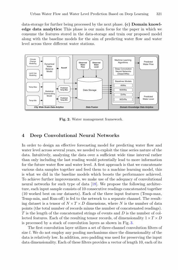
Urban Water Flow and Water Level Prediction Based on Deep Learning 321
data-storage for further being processed by the next phase. (c) Domain knowl-edge data analytics: This phase is our main focus for the paper in which weconsume the features stored in the data-storage and train our proposed modelalong with the baseline models for the aim of predicting water flow and waterlevel across three different water stations.
Climate Change Modeling
Land Use Modeling
Dynamical Water
Balance Model
Runoff
Statistical Downscaling
Model
Temp-Max
Temp-Min
Predicted Temp-Max
Predicted Temp-Min
Data Storage
Observed Water Flow
ObservedWater Level
Predicted Water Flow
Predicted Water Level
Machine Learning Algorithms
City Wide Scale Data Anlytics Data Fusion Domain Knowledge Data Anlytics
Deep Convolution Neural Networks
(DeepCNNs)
ANNs
WANNs
SVRs
WSVRs
Baselines Models
Fig. 2. Water management framework.
4 Deep Convolutional Neural Networks
In order to design an effective forecasting model for predicting water flow andwater level across several years, we needed to exploit the time series nature of thedata. Intuitively, analyzing the data over a sufficient wide time interval ratherthan only including the last reading would potentially lead to more informationfor the future water flow and water level. A first approach is that we concatenatevarious data samples together and feed them to a machine learning model, thisis what we did in the baseline models which boosts the performance achieved.To achieve further improvements, we make use of the adequacy of convolutionalneural networks for such type of data [18]. We propose the following architec-ture, each input sample consists of 10 consecutive readings concatenated together(10 worked best on our datasets). Each of the three input features (Temp-max,Temp-min, and Run-off) is fed to the network to a separate channel. The result-ing dataset is a tensor of N ×T ×D dimensions, where N is the number of datapoints (the total number of records minus the number of concatenated readings).T is the length of the concatenated strings of events and D is the number of col-lected features. Each of the resulting tensor records, of dimensionality 1×T ×Dis processed by a stack of convolution layers as shown in Fig. 3.
The first convolution layer utilizes a set of three-channel convolution filters ofsize l. We do not employ any pooling mechanisms since the dimensionality of thedata is relatively low. In addition, zero padding was used for preserving the inputdata dimensionality. Each of these filters provides a vector of length 10, each of its
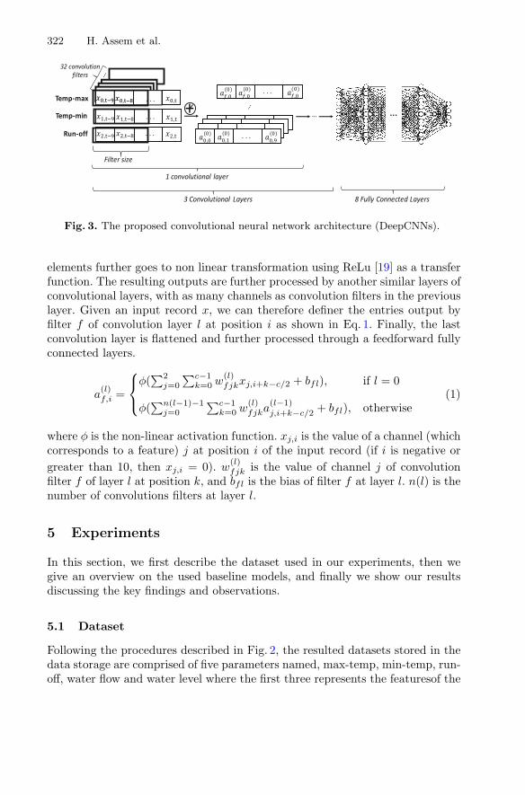
322 H. Assem et al.
Fig. 3. The proposed convolutional neural network architecture (DeepCNNs).
elements further goes to non linear transformation using ReLu [19] as a transferfunction. The resulting outputs are further processed by another similar layers ofconvolutional layers, with as many channels as convolution filters in the previouslayer. Given an input record x, we can therefore definer the entries output byfilter f of convolution layer l at position i as shown in Eq. 1. Finally, the lastconvolution layer is flattened and further processed through a feedforward fullyconnected layers.
a(l)f,i =
⎧⎨
⎩
φ(∑2
j=0
∑c−1k=0 w
(l)fjkxj,i+k−c/2 + bfl), if l = 0
φ(∑n(l−1)−1
j=0
∑c−1k=0 w
(l)fjka
(l−1)j,i+k−c/2 + bfl), otherwise
(1)
where φ is the non-linear activation function. xj,i is the value of a channel (whichcorresponds to a feature) j at position i of the input record (if i is negative orgreater than 10, then xj,i = 0). w
(l)fjk is the value of channel j of convolution
filter f of layer l at position k, and bfl is the bias of filter f at layer l. n(l) is thenumber of convolutions filters at layer l.
5 Experiments
In this section, we first describe the dataset used in our experiments, then wegive an overview on the used baseline models, and finally we show our resultsdiscussing the key findings and observations.
5.1 Dataset
Following the procedures described in Fig. 2, the resulted datasets stored in thedata storage are comprised of five parameters named, max-temp, min-temp, run-off, water flow and water level where the first three represents the featuresof the

Urban Water Flow and Water Level Prediction Based on Deep Learning 323
trained models while the later two represents the outputs of the models. Theused parameters can be defined as follows:
– max-temp, min-temp: These are the highest and lowest temperaturesrecorded in ◦C during each day in the dataset.
– run-off: Runoff is described as the part of the water cycle that flows over landas surface water instead of being absorbed into groundwater or evaporatingand is measured in mm.
– water flow: Water flow (streamflow) is the volume of water that movesthrough a specific point in a stream during a given period of time (one dayin our case) and is measured in m3/sec.
– water level: This parameter indicates the maximum height reached by thewater in the river during the day and is measured in m.
The previous parameters in the dataset are for 30-years (1983–2013) resultingin 11,392 samples where each sample represents a day. The datasets formulatedrelated to three different water hydrometric stations named, Inny, lower-shannon,and suck.
5.2 Baselines
In this section we describe the baseline models that have been developed forassessing the performance of the proposed deep convolutional neural network. Wechoose two very popular ordinary machine learning algorithms that has alreadyshown success in hyrdology, Artificial Neural Networks (ANNs) [8] and SupportVector Machines (SVMs) [4]. In addition, we choose two wavelet transformationmodels that have shown stable outcomes and in particular for the time-seriesforecasting problems, Wavelet-ANNs (WANNs) and Wavelet-SVMs (WSVMs).
– ANNs: We developed three layer feed-forward neural network employingbackpropogation algorithm. An automated RapidMinder algorithm proposedin [17] is utilized for optimizing the number of neurons in the hidden layerwith setting the number of epochs to 500, learning rate to 0.1 and momentumto 0.1 as well.
– SVMs: We developed SVM with non-linear dot kernel which requires twoparameters to be configured by the user, namely cost (C) and epsilon (ε). Weset C to 0.0001 and ε to 0.001. The selected combination was adjusted to themost precision that could be acquired through a trial and error process for amore localized optimization for the model parameters.
We used Discrete Wavelet Transforms (DWTs) to decompose the original timeseries into a time-frequency representation at different scales (wavelet sub-timesseries). In this type of baselines, we set the level of decomposition to 3, twolevels of details and one level of approximations. The signals were decomposedusing the redundant trous algorithm [5] in conjunction with the non-symmetricdb1 wavelet as the mother function2. Three sets of wavelet sub-time series were2 The using of the atrous algorithm with the db1 wavelet mother function is a result
of the optimizing Python Wavelet tool [9].
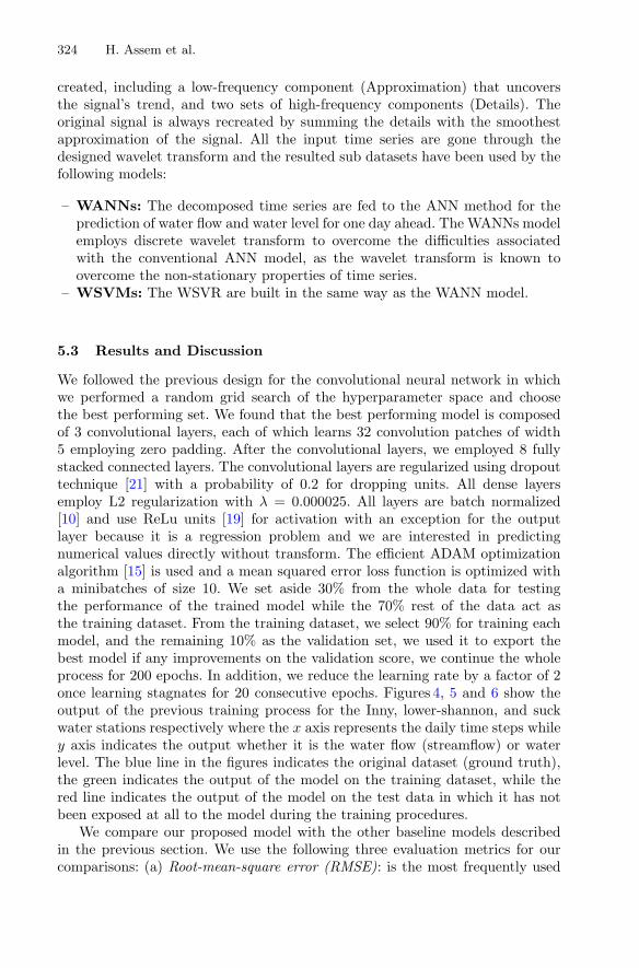
324 H. Assem et al.
created, including a low-frequency component (Approximation) that uncoversthe signal’s trend, and two sets of high-frequency components (Details). Theoriginal signal is always recreated by summing the details with the smoothestapproximation of the signal. All the input time series are gone through thedesigned wavelet transform and the resulted sub datasets have been used by thefollowing models:
– WANNs: The decomposed time series are fed to the ANN method for theprediction of water flow and water level for one day ahead. The WANNs modelemploys discrete wavelet transform to overcome the difficulties associatedwith the conventional ANN model, as the wavelet transform is known toovercome the non-stationary properties of time series.
– WSVMs: The WSVR are built in the same way as the WANN model.
5.3 Results and Discussion
We followed the previous design for the convolutional neural network in whichwe performed a random grid search of the hyperparameter space and choosethe best performing set. We found that the best performing model is composedof 3 convolutional layers, each of which learns 32 convolution patches of width5 employing zero padding. After the convolutional layers, we employed 8 fullystacked connected layers. The convolutional layers are regularized using dropouttechnique [21] with a probability of 0.2 for dropping units. All dense layersemploy L2 regularization with λ = 0.000025. All layers are batch normalized[10] and use ReLu units [19] for activation with an exception for the outputlayer because it is a regression problem and we are interested in predictingnumerical values directly without transform. The efficient ADAM optimizationalgorithm [15] is used and a mean squared error loss function is optimized witha minibatches of size 10. We set aside 30% from the whole data for testingthe performance of the trained model while the 70% rest of the data act asthe training dataset. From the training dataset, we select 90% for training eachmodel, and the remaining 10% as the validation set, we used it to export thebest model if any improvements on the validation score, we continue the wholeprocess for 200 epochs. In addition, we reduce the learning rate by a factor of 2once learning stagnates for 20 consecutive epochs. Figures 4, 5 and 6 show theoutput of the previous training process for the Inny, lower-shannon, and suckwater stations respectively where the x axis represents the daily time steps whiley axis indicates the output whether it is the water flow (streamflow) or waterlevel. The blue line in the figures indicates the original dataset (ground truth),the green indicates the output of the model on the training dataset, while thered line indicates the output of the model on the test data in which it has notbeen exposed at all to the model during the training procedures.
We compare our proposed model with the other baseline models describedin the previous section. We use the following three evaluation metrics for ourcomparisons: (a) Root-mean-square error (RMSE): is the most frequently used
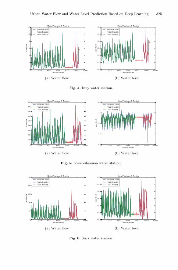
Urban Water Flow and Water Level Prediction Based on Deep Learning 325
Fig. 4. Inny water station.
Fig. 5. Lower-shannon water station.
Fig. 6. Suck water station.
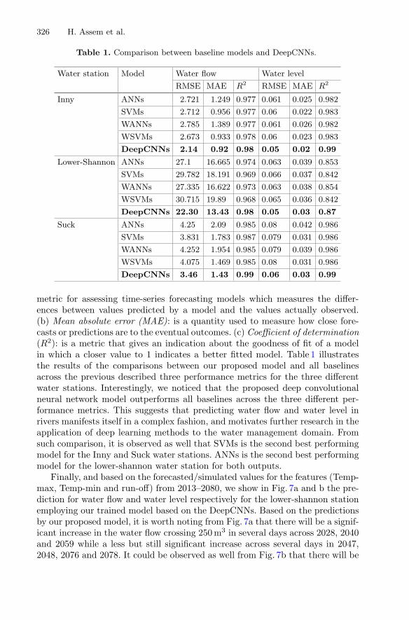
326 H. Assem et al.
Table 1. Comparison between baseline models and DeepCNNs.
Water station Model Water flow Water level
RMSE MAE R2 RMSE MAE R2
Inny ANNs 2.721 1.249 0.977 0.061 0.025 0.982
SVMs 2.712 0.956 0.977 0.06 0.022 0.983
WANNs 2.785 1.389 0.977 0.061 0.026 0.982
WSVMs 2.673 0.933 0.978 0.06 0.023 0.983
DeepCNNs 2.14 0.92 0.98 0.05 0.02 0.99
Lower-Shannon ANNs 27.1 16.665 0.974 0.063 0.039 0.853
SVMs 29.782 18.191 0.969 0.066 0.037 0.842
WANNs 27.335 16.622 0.973 0.063 0.038 0.854
WSVMs 30.715 19.89 0.968 0.065 0.036 0.842
DeepCNNs 22.30 13.43 0.98 0.05 0.03 0.87
Suck ANNs 4.25 2.09 0.985 0.08 0.042 0.986
SVMs 3.831 1.783 0.987 0.079 0.031 0.986
WANNs 4.252 1.954 0.985 0.079 0.039 0.986
WSVMs 4.075 1.469 0.985 0.08 0.031 0.986
DeepCNNs 3.46 1.43 0.99 0.06 0.03 0.99
metric for assessing time-series forecasting models which measures the differ-ences between values predicted by a model and the values actually observed.(b) Mean absolute error (MAE): is a quantity used to measure how close fore-casts or predictions are to the eventual outcomes. (c) Coefficient of determination(R2): is a metric that gives an indication about the goodness of fit of a modelin which a closer value to 1 indicates a better fitted model. Table 1 illustratesthe results of the comparisons between our proposed model and all baselinesacross the previous described three performance metrics for the three differentwater stations. Interestingly, we noticed that the proposed deep convolutionalneural network model outperforms all baselines across the three different per-formance metrics. This suggests that predicting water flow and water level inrivers manifests itself in a complex fashion, and motivates further research in theapplication of deep learning methods to the water management domain. Fromsuch comparison, it is observed as well that SVMs is the second best performingmodel for the Inny and Suck water stations. ANNs is the second best performingmodel for the lower-shannon water station for both outputs.
Finally, and based on the forecasted/simulated values for the features (Temp-max, Temp-min and run-off) from 2013–2080, we show in Fig. 7a and b the pre-diction for water flow and water level respectively for the lower-shannon stationemploying our trained model based on the DeepCNNs. Based on the predictionsby our proposed model, it is worth noting from Fig. 7a that there will be a signif-icant increase in the water flow crossing 250 m3 in several days across 2028, 2040and 2059 while a less but still significant increase across several days in 2047,2048, 2076 and 2078. It could be observed as well from Fig. 7b that there will be

Urban Water Flow and Water Level Prediction Based on Deep Learning 327
a significant rise of water level crossing 33.4 m in several days in 2021 and bitless in 2032, 2044, 2045 and others as well. These results should be very usefulfor further being assessed by water authorities for building mitigation plans forthe impact of such increase as well as better planning for water allocation acrossvarious competing users.
Fig. 7. Predictions of water flow and water level for lower-shannon water station from2013–2080 using the DeepCNNs proposed model.
6 Conclusion and Outlook
This paper presents the application of a new data-driven methods for model-ing and predicting daily water flow and water level on the catchment scale forthe Shannon river in Ireland. We have designed a deep convolutional networkarchitecture to exploit the time-series nature of the data. Using several featurescaptured at real across three various water stations, we have shown that the pro-posed convolutional network outperforms other four well-known time series fore-casting models (ANNs, SVMs, WANNs and WSVMs). The inputs to the modelsconsist of a combination of 30-years daily time series data sets (1983–2013),which can be divided between observed data sets (maximum temperature, min-imum temperature, water level and water flow) and simulated data set, runoff.Based on the proposed deep convolutional network model, we further show thepredictions of the water flow and water level for the lower-shannon water stationfrom the duration of 2013–2080. Our proposed solution should be very useful forwater authorities in the future allocation of water resources among competingusers such as agriculture, demotic and power stations. In addition, it could for-mulate the basis of a decision support system by setting thresholds on water flowand water level predictions for the sake of creating accurate emergency alarmsfor capturing any expected abnormalities for the Shannon river.
References
1. Beven, K.J., et al.: Streamflow Generation Processes. IAHS Press, Wallingford(2006)
2. Chattopadhyay, P.B., Rangarajan, R.: Application of ann in sketching spatial non-linearity of unconfined aquifer in agricultural basin. Agric. Water Manag. 133,81–91 (2014)

328 H. Assem et al.
3. Daniell, T.: Neural networks. Applications in hydrology and water resources engi-neering. In: National Conference Publication - Institute of Engineers. Australia(1991)
4. Deka, P.C., et al.: Support vector machine applications in the field of hydrology:a review. Appl. Soft Comput. 19, 372–386 (2014)
5. Dutilleux, P.: An implementation of the algorithme atrous to compute the wavelettransform. In: Combes, J.M., Grossmann, A., Tchamitchian, P. (eds.) Wavelets.IPTI, pp. 298–304. Springer, Heidelberg (1989). https://doi.org/10.1007/978-3-642-75988-8 29
6. Gharbia, S.S., Alfatah, S.A., Gill, L., Johnston, P., Pilla, F.: Land use scenariosand projections simulation using an integrated gis cellular automata algorithms.Model. Earth Syst. Environ. 2(3), 151 (2016)
7. Gharbia, S.S., Gill, L., Johnston, P., Pilla, F.: Multi-GCM ensembles performancefor climate projection on a GIS platform. Model. Earth Syst. Environ. 2(2), 1–21(2016)
8. Govindaraju, R.S., Rao, A.R.: Artificial Neural Networks in Hydrology, vol. 36.Springer Science & Business Media, Heidelberg (2013). https://doi.org/10.1007/978-94-015-9341-0
9. Hanke, M., Halchenko, Y.O., Sederberg, P.B., Hanson, S.J., Haxby, J.V., Pollmann,S.: PyMVPA: a python toolbox for multivariate pattern analysis of FMRI data.Neuroinformatics 7(1), 37–53 (2009)
10. Ioffe, S., Szegedy, C.: Batch normalization: accelerating deep network training byreducing internal covariate shift. arXiv preprint arXiv:1502.03167 (2015)
11. Karran, D.J., Morin, E., Adamowski, J.: Multi-step streamflow forecasting usingdata-driven non-linear methods in contrasting climate regimes. J. Hydroinformatics16(3), 671–689 (2014)
12. Kenabatho, P., Parida, B., Moalafhi, D., Segosebe, T.: Analysis of rainfall andlarge-scale predictors using a stochastic model and artificial neural network forhydrological applications in Southern Africa. Hydrol. Sci. J. 60(11), 1943–1955(2015)
13. Khan, M.S., Coulibaly, P.: Application of support vector machine in lake waterlevel prediction. J. Hydrol. Eng. 11(3), 199–205 (2006)
14. Kim, T.W., Valdes, J.B.: Nonlinear model for drought forecasting based on a con-junction of wavelet transforms and neural networks. J. Hydrol. Eng. 8(6), 319–328(2003)
15. Kingma, D., Ba, J.: ADAM: a method for stochastic optimization. arXiv preprintarXiv:1412.6980 (2014)
16. Kisi, O., Cimen, M.: A wavelet-support vector machine conjunction model formonthly streamflow forecasting. J. Hydrol. 399(1), 132–140 (2011)
17. Klinkenberg, R.: RapidMiner: Data Mining Use Cases and Business AnalyticsApplications. Chapman and Hall/CRC, Boca Raton (2013)
18. LeCun, Y., Bengio, Y., et al.: Convolutional networks for images, speech, and timeseries. In: The Handbook of Brain Theory and Neural Networks, vol. 3361, No. 10(1995)
19. Nair, V., Hinton, G.E.: Rectified linear units improve restricted Boltzmannmachines. In: Proceedings of the 27th International Conference on Machine Learn-ing (ICML 2010), pp. 807–814 (2010)
20. Sivakumar, B.: Forecasting monthly streamflow dynamics in the Western UnitedStates: a nonlinear dynamical approach. Environ. Model. Softw. 18(8), 721–728(2003)

Urban Water Flow and Water Level Prediction Based on Deep Learning 329
21. Srivastava, N., Hinton, G.E., Krizhevsky, A., Sutskever, I., Salakhutdinov, R.:Dropout: a simple way to prevent neural networks from overfitting. J. Mach. Learn.Res. 15(1), 1929–1958 (2014)
22. Zheng, Y.: Methodologies for cross-domain data fusion: an overview. IEEE Trans.Big Data 1(1), 16–34 (2015)

Using Machine Learning for Labour MarketIntelligence
Roberto Boselli1,2, Mirko Cesarini1,2, Fabio Mercorio1,2(B),and Mario Mezzanzanica1,2
1 Department of Statistics and Quantitative Methods, University of Milano-Bicocca,Milan, Italy
[email protected] CRISP Research Centre, University of Milano-Bicocca, Milan, Italy
Abstract. The rapid growth of Web usage for advertising job positionsprovides a great opportunity for real-time labour market monitoring.This is the aim of Labour Market Intelligence (LMI), a field that isbecoming increasingly relevant to EU Labour Market policies design andevaluation. The analysis of Web job vacancies, indeed, represents a com-petitive advantage to labour market stakeholders with respect to classicalsurvey-based analyses, as it allows for reducing the time-to-market of theanalysis by moving towards a fact-based decision making model. In thispaper, we present our approach for automatically classifying million Webjob vacancies on a standard taxonomy of occupations. We show how thisproblem has been expressed in terms of text classification via machinelearning. Then, we provide details about the classification pipelines weevaluated and implemented, along with the outcomes of the validationactivities. Finally, we discuss how machine learning contributed to theLMI needs of the European Organisation that supported the project.
Keywords: Machine learning · Text classificationGovernmental application
1 Introduction
In recent years, the European Labour demand conveyed through specialised Webportals and services has grown exponentially. This also contributed to introducethe term “Labour Market Intelligence” (LMI), that refers to the use and designof AI algorithms and frameworks to analyse Labour Market Data for supportingdecision making. This is the case ofWeb job vacancies, that are job advertisementscontaining two main text fields: a title and a full description. The title shortlysummarises the job position, while the full description field usually includes theposition details and the relevant skills that the employee should hold.
There is a growing interest in designing and implementing real LMI applica-tions to Web Labour Market data for supporting the policy design and evalu-ation activities through evidence-based decision-making. In 2010 the Europeanc© Springer International Publishing AG 2017Y. Altun et al. (Eds.): ECML PKDD 2017, Part III, LNAI 10536, pp. 330–342, 2017.https://doi.org/10.1007/978-3-319-71273-4_27

Machine Learning for LMI 331
Commission has published the communication “A new impetus for EuropeanCooperation in Vocational Education and Training (VET) to support the Europe2020 strategy”,1 aimed at promoting education systems in general, and VET inparticular. In 2016, the European Commission’s highlighted the importance ofVocational and Educational activities, as they are “valued for fostering job-specific and transversal skills, facilitating the transition into employment andmaintaining and updating the skills of the workforce according to sectorial,regional, and local needs”.2 In 2016, the EU and Eurostat launched the ESSnetBig Data project, involving 22 EU member states with the aim of “integratingbig data in the regular production of official statistics, through pilots exploringthe potential of selected big data sources and building concrete applications”.
The rationale behind all these initiatives is that reasoning over Web jobvacancies represents an added value for both public and private labour mar-ket operators to deeply understand the Labour Market dynamics, occupations,skills, and trends: (i) by reducing the time-to-market with respect to classicalsurvey-based analyses (results of official Labour Market surveys actually requireup to one year before being available); (ii) by overcoming the linguistic bound-aries through the use of standard classification systems rather than proprietaryones; (iii) by representing the resulting knowledge over several dimensions (e.g.,territory, sectors, contracts, etc.) at different level of granularity and (iv) byevaluating and comparing international labour markets to support fact-baseddecision making.
Contribution. In this paper we present our approach for classifying Web jobvacancies, we designed and realised within a research call-for-tender3 for theCedefop EU organisation4. Specifically, the goal of this project was twofold:first, the evaluation of the effectiveness of using Web Job vacancies for LMIactivities through a feasibility study, second, the realisation of a working pro-totype that collects and analyses Web job vacancies over 5 Countries (UnitedKingdom, Ireland, Czech Republic, Italy, and Germany) for obtaining near-realtime labour market information. Here we focus on the classification task show-ing the performances achieved by three classification pipelines we evaluated forrealising the system.
We begin by discussing related work in Sect. 2. In Sect. 3 we discuss howthe problem of classifying Web job vacancies has been solved through machinelearning, providing details on the feature extraction techniques used. Section 4
1 Publicly available at https://goo.gl/Goluxo.2 The Commission Communication “A New Skills Agenda for Europe” COM (2016)
381/2, available at https://goo.gl/Shw7bI.3 “Real-time Labour Market information on skill requirements: feasibility study and
working prototype”. Cedefop Reference number AO/RPA/VKVET-NSOFRO/Real-time LMI/010/14. Contract notice 2014/S 141-252026 of 15/07/2014 https://goo.gl/qNjmrn.
4 Cedefop European agency supports the development of European Vocational Educa-tion and Training (VET) policies and contributes to their implementation - http://www.cedefop.europa.eu/.
332 R. Boselli et al.
provides the experimental results about the evaluation of three distinct pipelinesemployed. Section 5 concludes the paper and describes the ongoing research.
2 Related Work
Labour Market Intelligence is an emerging cross-disciplinary field of studies thatis gaining research interests in both industrial and academic communities.
Industries. Information extraction from unstructured texts in the labour marketdomain mainly focused on the e-recruitment process (see, e.g., [19]) attemptingto support or automate the resume management by matching candidate profileswith job descriptions using machine learning approaches [11,30,32]. Concern-ing companies, their need to automatize Human Resource (HR) departmentactivities is strong; as a consequence, a growing amount of commercial skill-matching products have been developed in the last years, for instance, Burning-Glass, Workday, Pluralsight, EmployInsight, and TextKernel. To date, the onlycommercial solution that uses international standard taxonomies is Janzz: a Webbased platform to match labour demand and supply in both public and privatesectors. It also provides APIs access to its knowledge base, but it is not aimedat classifying job vacancies. Worth of mentioning is Google Job Search API, apay-as-you-go service announced in 2016 for classifying job vacancies throughthe Google Machine Learning service over O*NET, that is the US standardoccupation taxonomy. Though this commercial service is still a closed alpha, itis quite promising and also sheds the light on the needs for reasoning with Webjob vacancies using a common taxonomy as baseline.
Literature. Since the early 1990s, text classification (TC) has been an activeresearch topic. It has been defined as “the activity of labelling natural lan-guage texts with thematic categories from a predefined set” [29]. Most populartechniques are based on the machine learning paradigm, according to which anautomatic text classifier is created by using an inductive process able to learn,from a set of pre-classified documents, the characteristics of the categories ofinterest.
In the recent literature, text classification has proven to give good results incategorizing many real-life Web-based data such as, for instance, news and socialmedia [15,33], and sentiment analysis [20,25]. To the best of our knowledge, textclassifiers have not been applied yet to the classification of Web job vacanciespublished on several Web sites for analysing the Web job market of a geographicalarea, and this system is the first example in this direction.
All these approaches are quite relevant and effective, and they also make evi-dence of the importance of the Web for labour market information. Nonetheless,they differ from our approach in two aspects. First, we aim to classify job vacan-cies according to a target classification system for building a (language inde-pendent) knowledge base for analyses purposes, rather than matching resumeson job vacancies. Furthermore, resumes are usually accurately written by can-didates whilst Web advertisements are written in a less accurate way, and this

Machine Learning for LMI 333
quality issue might have unpredictable effects on the information derived fromthem (see, e.g. [6,9,21,22] for practical applications). Second, the system aimsat producing analyses based on standard taxonomies to support the fact-baseddecision making activities of several stakeholders.
3 Text Classification in LMI
The Need for a Standard Occupations Taxonomy. The use of proprietary andlanguage-dependent taxonomies can prevent the effective monitoring and evalu-ation of Labour Market dynamics across national borders. For these reasons, agreat effort has been made by International organisations for designing standardclassifications systems, that would act as a lingua-franca for the Labour Marketto overcome the linguistic boundaries as well. One of the most important classi-fication system designed for this purposes is ISCO: The International StandardClassification of Occupations has been developed by the International LabourOrganization as a four-level classification that represents a standardised way fororganising the labour market occupations. In 2014, ISCO has been extendedthrough ESCO: the multilingual classification system of European Skills, Com-petences, Qualifications and Occupations, that is emerging as the Europeanstandard for supporting the whole labour market intelligence over 24 EU lan-guages. Basically, the ESCO data model includes the ISCO hierarchical structureas a whole and extends it through a taxonomy of skills, competences and quali-fications.
3.1 The Classification Task
Text categorisation aims at assigning a Boolean value to each pair (dj , ci) ∈D × C where D is a set of documents and C a set of predefined categories. Atrue value assigned to (dj , ci) indicates document dj to be set under the categoryci, while a false value indicates dj cannot be assigned under ci. In our scenario,we consider a set of job vacancies J as a collection of documents each of whichhas to be assigned to one (and only one) ISCO occupation code. We can modelthis problem as a text classification problem, relying on the definition of [29].
Formally speaking, let J = {J1, . . . , Jn} be a set of job vacancies, the classi-fication of J under the ESCO classification system consists of |O| independentproblems of classifying each job vacancy J ∈ J under a given ESCO occupationcode oi for i = 1, . . . , |O|. Then, a classifier is a function ψ : J × O → {0, 1}that approximates an unknown target function ψ : J × O → {0, 1}. Clearly, aswe deal with a single-label classifier, ∀j ∈ J the following constraint must hold:∑
o∈O ψ(j, o) = 1.In this paper, job vacancies are classified according to the 4th level of the
ISCO taxonomy (and the corresponding multilingual concepts of the ESCOontology) as further detailed in the next sections. The choice of the ISCO 4th
level (also referred as ISCO 4 digits classification) is a trade-off between thegranularity of occupations (the more digits the better) and the effort to develop

334 R. Boselli et al.
an automatic classifier (the fewer digits the better). The job vacancy classifica-tion is translated into a supervised machine learning text classification problem,namely a multiclass single label classification problem i.e., a job offer is classifiedto one and only one 4 digits ISCO code over a set of 436 available ones.
Within this project we decided to use titles for occupation classification.Indeed, in our very preliminary studies [2] we experimentally observed that titlesare often concise and highly focused on describing the proposed occupationswhile other topics are hardly dealt, making titles suitable for the classificationtask.
3.2 Feature Extraction
Two feature extraction methods have been evaluated for classifying job occupa-tion, namely: Bag of Word Approach, and Word2Vec, that we describe in thefollowing.
Bag of Word Feature Extraction. Titles were pre-processed according to thefollowing steps: (i) html tag removal, (ii) html entities and symbol replacement,(iii) tokenization, (iv) lower case reduction, (v) stop words removal (using thestop-words list provided by the NLTK framework [5]), (vi) stemming (using theSnowball stemmer), (vii) n-grams frequency computation (actually, unigram andbigram frequencies were computed, n-grams which appear less than 4 times orthat appear in more than 30% of the documents are discarded, since they arenot significant for classification). Each title is pre-processed according to theprevious steps and is transformed into a set of n-gram frequencies.
Word2Vec Feature Extraction. Each word in a title was replaced by a cor-responding vector of an n-dimensional space. We used a vector representation ofwords belonging to the family of neural language models [3] and specifically weused the Word2Vec [23,24] representation.
In neural language models, every word is mapped to a unique vector, givena word w and its context k (n words nearby w), the concatenation or sum ofthe vectors of the context words is then used as features for prediction of theword w [24]. This problem can be viewed as a machine learning problem wheren context words are fed into a neural network that should be trained to predictthe corresponding word, according to the Continuous Bag of Words (CBOW)model proposed in [23].
The word vector representations are the coefficient of the internal layers ofthe neural network, for more details the interested reader can refer to [24]. Theword vectors are also called word embeddings.
After the training ends, words with similar meaning are mapped to a similarposition in the vector space [23]. For example, “powerful” and “strong” are closeto each other, whereas “powerful” and “Paris” are more distant. The word vectordifferences also carry meaning.
We used the GENSIM [27] implementation of Word2Vec to identify the vec-tor representations of the words. Since Word2Vec requires huge text corpora forproducing meaningful vectors, we used all the downloaded job vacancies to train

Machine Learning for LMI 335
the Word2Vec (the unlabelled dataset, about 6 Million of job vacancies, as out-lined in Sect. 4.1). The 6 Million job vacancy texts underwent the steps from (i)to (vi) of the processing pipeline described in Subsect. 3.2 before being used fortraining the Word2Vec model. Actually, the Wod2Vec model was trained usingvectors of size equals to 300 using the CBOW training algorithm.
The Word2Vec embeddings were used to process the titles of the labelleddataset introduced in Sect. 4.1 as follows: steps from (i) to (vi) of the processingpipeline described in Subsect. 3.2 were executed on titles. The first 15 tokensof titles where considered (i.e., tokens exceeding the 15th were dropped, as theaffected titles account for less than 0.2% of total vacancies). Each word in thetitle was replaced by the corresponding (word) vector, e.g., given a set of n titleseach one composed by 15 words, the output of the substitution can be viewed asa 3-dimensional array (e.g., a 3-dimensional matrix or a 3-dimensional tensor)of the shape: [n documents, 15, word vector dimension].
4 Experimental Results
This section introduces the evaluation performed on the several classificationpipelines and the dataset used.
4.1 Datasets
Two datasets have been considered in the experiments outlined in this section:
Labelled. A set of 35,936 job vacancies manually labelled using 4 digits ISCOcode. Not all the 4 digits ISCO occupations are present in the dataset, only271 out of 436 ISCO codes were actually found. It is worth to mention thatISCO tries to categorize all possible occupations, but some are hardly foundon the Web (e.g., 9624 Water and firewood collectors5). The interested readercan refer to [13] for further information.
Unlabelled. A set of 6,005,916 unlabelled vacancies. The vacancies have beencollected for one year scraping 7 web sites focusing on the UK and Irish JobMarket. For each vacancy both a title and a full description is available.
The labelled dataset was used to train a classifier to be used later to identifythe ISCO occupations on the unlabelled vacancy dataset. The latter was used tocompute the Word2Vec word embeddings.
In the following sections, the classification pipelines we have evaluated areintroduced. For evaluation purposes, the labelled dataset was randomly split intotrain and test (sub)sets containing respectively 75% and 25% of the vacancies.The vacancies of each ISCO code were distributed in the two subsets using thesame proportions.
5 Tasks include cutting and collecting wood from forests for sale in market or for ownconsumption . . . drawing water from wells, rivers or ponds, etc. for domestic use.

336 R. Boselli et al.
4.2 Classification Pipelines
This subsection will introduce the several classification pipelines which havebeen evaluated for classifying job vacancies. Each pipeline has parameters whoseoptimal values have been found performing a Grid Search as detailed in Sect. 4.3.
BoW - SVM. The BoW feature extraction pipeline (described in Sect. 3.2) wasused on the (labelled) training dataset and the results were used to feed twoclassifiers, namely Linear SVM and Gaussian SVM, the latter also known asradial basis function (RBF) SVM kernel [8]. They will be called LinearSVM andRBF SVM hereafter.
According to [14], SVM is well suited to the particular properties of texts,namely high dimensional feature spaces, few irrelevant features (dense con-cept vector), and sparse instance vectors. The parameters evaluated duringthe grid search are C ∈ {0.01, 0.1, 1, 10, 100} for LinearSVM classifier, whileC ∈ {0.01, 0.1, 1}× Gamma ∈ {0.1, 1, 10} for RBF SVM.
BoW - Neural Network. The BoW feature extraction pipeline (described inSect. 3.2) was also used to feed the fully connected neural networks describedbelow. Each neural network has an input of size 5,820 (the number of featuresproduced by the feature extraction pipeline) and an output of size 271 (thenumber of ISCO codes in the training set). Each layer (if not otherwise specified)use the Linear Rectifier as non linearity, excluding the last layer which usesSoftmax. In the networks described below each fully connected layer is precededby a batch normalization layer [12], whose purpose is to accelerate the networktraining (and it doesn’t have an effect on the classification performances).
– (FCNN1) is a 4 layer neural network having 2 hidden layers: a batch normal-ization and a fully connected layer of size 3, 000.
– (FCNN2) is a 5 layer neural network, having 4 hidden layers: two fully con-nected layers respectively of 3, 900 and 2, 000 neuron size, each one precededby a batch normalization layer.
Word2Vec - Convolutional Neural Networks. Convolutional Neural Net-works (CNNs) are a type of Neural Network where the first layers act as filtersto identify patterns in the input data set and consequently to work on a moreabstract representation of the input. CNNs were originally employed in Com-puter Vision, the interested reader can refer to [17,18,28] for more details. CNNshave been employed to solve text classification tasks [7,16].
In this paper, we evaluated the convolutional neural network described inTable 1 over the results of the Word2Vec pipeline described in Sect. 3.2.
The first two convolutional layers perform a convolution over the Word2Vecfeatures producing as output respectively the results of 200 and 100 filters. Atthe end of the latter convolutional layer, each title can be viewed as a matrixof 15 × 100 (respectively, the number of words and the quantity of filter valuescomputed on each word embedding). The FeaturePoolLayer averages the 15values for each filter, at the end of this layer each title can be viewed as a vector
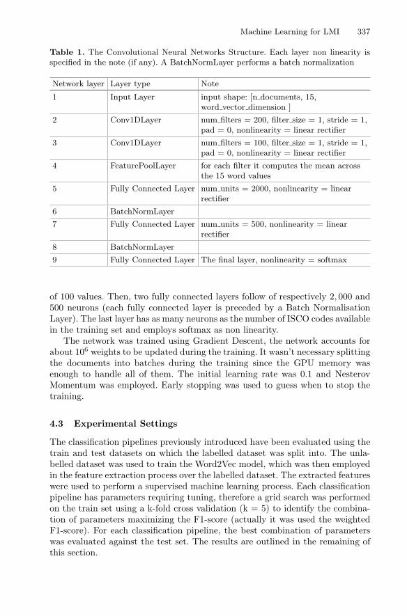
Machine Learning for LMI 337
Table 1. The Convolutional Neural Networks Structure. Each layer non linearity isspecified in the note (if any). A BatchNormLayer performs a batch normalization
Network layer Layer type Note
1 Input Layer input shape: [n documents, 15,word vector dimension ]
2 Conv1DLayer num filters = 200, filter size = 1, stride = 1,pad = 0, nonlinearity = linear rectifier
3 Conv1DLayer num filters = 100, filter size = 1, stride = 1,pad = 0, nonlinearity = linear rectifier
4 FeaturePoolLayer for each filter it computes the mean acrossthe 15 word values
5 Fully Connected Layer num units = 2000, nonlinearity = linearrectifier
6 BatchNormLayer
7 Fully Connected Layer num units = 500, nonlinearity = linearrectifier
8 BatchNormLayer
9 Fully Connected Layer The final layer, nonlinearity = softmax
of 100 values. Then, two fully connected layers follow of respectively 2, 000 and500 neurons (each fully connected layer is preceded by a Batch NormalisationLayer). The last layer has as many neurons as the number of ISCO codes availablein the training set and employs softmax as non linearity.
The network was trained using Gradient Descent, the network accounts forabout 106 weights to be updated during the training. It wasn’t necessary splittingthe documents into batches during the training since the GPU memory wasenough to handle all of them. The initial learning rate was 0.1 and NesterovMomentum was employed. Early stopping was used to guess when to stop thetraining.
4.3 Experimental Settings
The classification pipelines previously introduced have been evaluated using thetrain and test datasets on which the labelled dataset was split into. The unla-belled dataset was used to train the Word2Vec model, which was then employedin the feature extraction process over the labelled dataset. The extracted featureswere used to perform a supervised machine learning process. Each classificationpipeline has parameters requiring tuning, therefore a grid search was performedon the train set using a k-fold cross validation (k = 5) to identify the combina-tion of parameters maximizing the F1-score (actually it was used the weightedF1-score). For each classification pipeline, the best combination of parameterswas evaluated against the test set. The results are outlined in the remaining ofthis section.
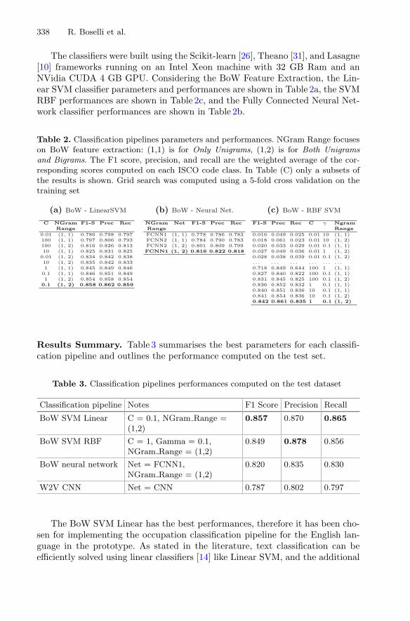
338 R. Boselli et al.
The classifiers were built using the Scikit-learn [26], Theano [31], and Lasagne[10] frameworks running on an Intel Xeon machine with 32 GB Ram and anNVidia CUDA 4 GB GPU. Considering the BoW Feature Extraction, the Lin-ear SVM classifier parameters and performances are shown in Table 2a, the SVMRBF performances are shown in Table 2c, and the Fully Connected Neural Net-work classifier performances are shown in Table 2b.
Table 2. Classification pipelines parameters and performances. NGram Range focuseson BoW feature extraction: (1,1) is for Only Unigrams, (1,2) is for Both Unigramsand Bigrams. The F1 score, precision, and recall are the weighted average of the cor-responding scores computed on each ISCO code class. In Table (C) only a subsets ofthe results is shown. Grid search was computed using a 5-fold cross validation on thetraining set
(a) BoW - LinearSVM
C NGram F1-S Prec RecRange
0.01 (1, 1) 0.786 0.798 0.797100 (1, 1) 0.797 0.806 0.793100 (1, 2) 0.816 0.826 0.81310 (1, 1) 0.825 0.831 0.825
0.01 (1, 2) 0.834 0.842 0.83810 (1, 2) 0.835 0.842 0.8331 (1, 1) 0.845 0.849 0.846
0.1 (1, 1) 0.846 0.851 0.8491 (1, 2) 0.854 0.858 0.854
0.1 (1, 2) 0.858 0.862 0.859
(b) BoW - Neural Net.
NGram Net F1-S Prec RecRangeFCNN1 (1, 1) 0.778 0.786 0.783FCNN2 (1, 1) 0.784 0.790 0.783FCNN2 (1, 2) 0.801 0.809 0.799FCNN1 (1, 2) 0.816 0.822 0.818
(c) BoW - RBF SVM
F1-S Prec Rec C γ NgramRange
0.016 0.049 0.025 0.01 10 (1, 1)0.018 0.061 0.023 0.01 10 (1, 2)0.020 0.033 0.029 0.01 0.1 (1, 1)0.027 0.049 0.036 0.01 1 (1, 2)0.028 0.038 0.039 0.01 0.1 (1, 2). . . . . . . . . . . . . . . . . .0.718 0.849 0.644 100 1 (1, 1)0.827 0.840 0.822 100 0.1 (1, 1)0.831 0.845 0.825 100 0.1 (1, 2)0.836 0.852 0.832 1 0.1 (1, 1)0.840 0.851 0.836 10 0.1 (1, 1)0.841 0.854 0.836 10 0.1 (1, 2)0.842 0.861 0.835 1 0.1 (1, 2)
Results Summary. Table 3 summarises the best parameters for each classifi-cation pipeline and outlines the performance computed on the test set.
Table 3. Classification pipelines performances computed on the test dataset
Classification pipeline Notes F1 Score Precision Recall
BoW SVM Linear C = 0.1, NGram Range =(1,2)
0.857 0.870 0.865
BoW SVM RBF C = 1, Gamma = 0.1,NGram Range = (1,2)
0.849 0.878 0.856
BoW neural network Net = FCNN1,NGram Range = (1,2)
0.820 0.835 0.830
W2V CNN Net = CNN 0.787 0.802 0.797
The BoW SVM Linear has the best performances, therefore it has been cho-sen for implementing the occupation classification pipeline for the English lan-guage in the prototype. As stated in the literature, text classification can beefficiently solved using linear classifiers [14] like Linear SVM, and the additional

Machine Learning for LMI 339
complexity of non-linear classification does not tend to pay for itself [1], exceptfor some special data sets. Considering the Word2Vec Convolutional Neural Net-work, the performances are shown in Table 3, the authors would have expectedbetter results, and the matter calls for further experiments.
4.4 Results Validation by EU Organisation
The project provided two main outcomes to the Cedefop EU Agency that sup-ported it. On one side, a feasibility study, that has not been addressed in thispaper, reporting some best practices identified by labour market experts involvedwithin the project and belonging to the ENRLMM.6 As a major result, theproject provided a working prototype that has been deployed at Cedefop in June2016 and it is currently running on the Cedefop Datacenter. In Fig. 1 we reporta snapshot from a demo dashboard that provides an overview of the occupa-tion trends over the period June-September 2015 collecting up to 700 K uniqueWeb job vacancies. To date, the system collected 7+ million job vacancies overthe 5 EU countries, and it is among a selection of research projects of Italianuniversities framed within a Big Data context [4].
Below we report an example of how the classified job vacancies could beused to support LMI monitoring, focusing only on 4-months scraping data. Onemight closely looks at the differences between countries in terms of labour marketdemands. Comparing UK against Italy, we can see that “Sales, Marketing anddevelopment managers” are the most requested occupations at ESCO (level 2)in the UK over this period whilst, rolling up on ESCO level 1 we can observethat “Professionals” are mainly asked in the “Information and Communication”sector, followed by “Administrative and support service activities” accordingto the NACE taxonomy. Furthermore, the type of contract is usually specifiedoffering permanent contracts. Differently, the Italian labour market, that has ajob vacancy posting rate ten times lower than UK over the same period, is lookingat Business Service Agents requested in the “Manufacturing” field offering oftentemporary contracts.
Interactive Demos. Due to the space restrictions, the dashboard in Fig. 1 andsome other demo dashboards have been made available online: Industry andOccupation Dashboard at https://goo.gl/bdqMkz, Time-Series Dashboard athttps://goo.gl/wwqjhz, and Occupations Dashboard at https://goo.gl/M1E6x9
Project Results Validation. Finally, the project results have been discussed andendorsed in a workshop which took place in Thessaloniki, in December 2015.7
The methodology and the results obtained have been validated as effective by
6 The Network on Regional Labour Market Monitoring, http://www.regionallabourmarketmonitoring.net/.
7 The Workshop agenda and participants list is available at https://goo.gl/71Oc7A.
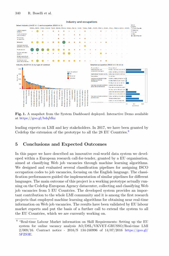
340 R. Boselli et al.
Fig. 1. A snapshot from the System Dashboard deployed. Interactive Demo availableat https://goo.gl/bdqMkz
leading experts on LMI and key stakeholders. In 2017, we have been granted byCedefop the extension of the prototype to all the 28 EU Countries.8
5 Conclusions and Expected Outcomes
In this paper we have described an innovative real-world data system we devel-oped within a European research call-for-tender, granted by a EU organisation,aimed at classifying Web job vacancies through machine learning algorithms.We designed and evaluated several classification pipelines for assigning ISCOoccupation codes to job vacancies, focusing on the English language. The classi-fication performances guided the implementation of similar pipelines for differentlanguages. The main outcome of this project is a working prototype actually run-ning on the Cedefop European Agency datacenter, collecting and classifying Webjob vacancies from 5 EU Countries. The developed system provides an impor-tant contribution to the whole LMI community and it is among the first researchprojects that employed machine learning algorithms for obtaining near real-timeinformation on Web job vacancies. The results have been validated by EU labourmarket experts and put the basis of a further call to extend the system to allthe EU Countries, which we are currently working on.
8 “Real-time Labour Market information on Skill Requirements: Setting up the EUsystem for online vacancy analysis AO/DSL/VKVET-GRUSSO/Real-time LMI2/009/16. Contract notice - 2016/S 134-240996 of 14/07/2016 https://goo.gl/5FZS3E.

Machine Learning for LMI 341
References
1. Aggarwal, C.C., Zhai, C.: A survey of text classification algorithms. In: Aggar-wal, C., Zhai, C. (eds.) Mining Text Data, pp. 163–222. Springer, Boston (2012).https://doi.org/10.1007/978-1-4614-3223-4 6
2. Amato, F., Boselli, R., Cesarini, M., Mercorio, F., Mezzanzanica, M., Moscato,V., Persia, F., Picariello, A.: Challenge: processing web texts for classifying joboffers. In: 2015 IEEE International Conference on Semantic Computing (ICSC),pp. 460–463 (2015)
3. Bengio, Y., Ducharme, R., Vincent, P., Jauvin, C.: A neural probabilistic languagemodel. J. Mach. Learn. Res. 3, 1137–1155 (2003)
4. Bergamaschi, S., Carlini, E., Ceci, M., Furletti, B., Giannotti, F., Malerba, D.,Mezzanzanica, M., Monreale, A., Pasi, G., Pedreschi, D., et al.: Big data researchin Italy: a perspective. Engineering 2(2), 163–170 (2016)
5. Bird, S., Klein, E., Loper, E.: Natural Language Processing with Python: AnalyzingText with the Natural Language Toolkit. O’Reilly Media Inc., Sebastopol (2009)
6. Boselli, R., Mezzanzanica, M., Cesarini, M., Mercorio, F.: Planning meets datacleansing. In: The 24th International Conference on Automated Planning andScheduling (ICAPS 2014), pp. 439–443. AAAI (2014)
7. Collobert, R., Weston, J.: A unified architecture for natural language processing:deep neural networks with multitask learning. In: The 25th International Confer-ence on Machine Learning, pp. 160–167. ICML, ACM (2008)
8. Cortes, C., Vapnik, V.: Support-vector networks. Mach. Learn. 20(3), 273–297(1995)
9. Dasu, T.: Data glitches: monsters in your data. In: Sadiq, S. (ed.) Handbook ofData Quality, pp. 163–178. Springer, Heidelberg (2013). https://doi.org/10.1007/978-3-642-36257-6 8
10. Dieleman, S., Schluter, J., Raffel, C., Olson, E., Sønderby, S.K., Nouri, D., et al.:Lasagne: first release, August 2015. https://doi.org/10.5281/zenodo.27878
11. Hong, W., Zheng, S., Wang, H.: Dynamic user profile-based job recommender sys-tem. In: Computer Science and Education (ICCSE). IEEE (2013)
12. Ioffe, S., Szegedy, C.: Batch normalization: Accelerating deep network training byreducing internal covariate shift. arXiv preprint arXiv:1502.03167 (2015)
13. International standard classification of occupations (2012). Accessed 11 Nov 201614. Joachims, T.: Text categorization with support vector machines: learning with
many relevant features. In: Nedellec, C., Rouveirol, C. (eds.) ECML 1998. LNCS,vol. 1398, pp. 137–142. Springer, Heidelberg (1998). https://doi.org/10.1007/BFb0026683
15. Khan, F.H., Bashir, S., Qamar, U.: TOM: Twitter opinion mining framework usinghybrid classification scheme. Decis. Support Syst. 57, 245–257 (2014)
16. Kim, Y.: Convolutional neural networks for sentence classification. arXiv preprintarXiv:1408.5882 (2014)
17. Krizhevsky, A., Sutskever, I., Hinton, G.E.: ImageNet classification with deep con-volutional neural networks. In: Advances in Neural Information Processing Systems25, pp. 1097–1105. Curran Associates, Inc. (2012)
18. Lee, H., Grosse, R., Ranganath, R., Ng, A.Y.: Convolutional deep belief networksfor scalable unsupervised learning of hierarchical representations. In: The 26thAnnual International Conference on Machine Learning, ICML 2009, pp. 609–616.ACM (2009)

342 R. Boselli et al.
19. Lee, I.: Modeling the benefit of e-recruiting process integration. Decis. SupportSyst. 51(1), 230–239 (2011)
20. Melville, P., Gryc, W., Lawrence, R.D.: Sentiment analysis of blogs by combininglexical knowledge with text classification. In: ACM SIGKDD International Con-ference on Knowledge Discovery and Data Mining. ACM (2009)
21. Mezzanzanica, M., Boselli, R., Cesarini, M., Mercorio, F.: Data quality sensitivityanalysis on aggregate indicators. In: Helfert, M., Francalanci, C., Filipe, J. (eds.)Proceedings of the International Conference on Data Technologies and Applica-tions, Data 2012, pp. 97–108. INSTICC (2012)
22. Mezzanzanica, M., Boselli, R., Cesarini, M., Mercorio, F.: A model-based evalua-tion of data quality activities in KDD. Inf. Process. Manag. 51(2), 144–166 (2015)
23. Mikolov, T., Chen, K., Corrado, G., Dean, J.: Efficient estimation of word repre-sentations in vector space. arXiv preprint arXiv:1301.3781 (2013)
24. Mikolov, T., Sutskever, I., Chen, K., Corrado, G.S., Dean, J.: Distributed repre-sentations of words and phrases and their compositionality. In: Advances in NeuralInformation Processing Systems, pp. 3111–3119 (2013)
25. Pang, B., Lee, L., Vaithyanathan, S.: Thumbs up?: sentiment classification usingmachine learning techniques. In: Proceedings of the ACL-02 Conference on Empir-ical Methods in Natural Language Processing, vol. 10, pp. 79–86. Association forComputational Linguistics (2002)
26. Pedregosa, F., Varoquaux, G., Gramfort, A., Michel, V., Thirion, B., Grisel, O.,Blondel, M., Prettenhofer, P., Weiss, R., Dubourg, V., Vanderplas, J., Passos, A.,Cournapeau, D., Brucher, M., Perrot, M., Duchesnay, E.: Scikit-learn: machinelearning in Python. J. Mach. Learn. Res. 12, 2825–2830 (2011)
27. Rehurek, R., Sojka, P.: Software framework for topic modelling with large cor-pora. In: Proceedings of the LREC 2010 Workshop on New Challenges for NLPFrameworks, pp. 45–50. ELRA, Valletta, May 2010. http://is.muni.cz/publication/884893/en
28. Schmidhuber, J.: Deep learning in neural networks: an overview. Neural Netw. 61,85–117 (2015)
29. Sebastiani, F.: Machine learning in automated text categorization. ACM Comput.Surv. (CSUR) 34(1), 1–47 (2002)
30. Singh, A., Rose, C., Visweswariah, K., Chenthamarakshan, V., Kambhatla, N.:Prospect: a system for screening candidates for recruitment. In: Proceedings of the19th ACM International Conference on Information and Knowledge Management,pp. 659–668. ACM (2010)
31. Theano Development Team: Theano: A Python framework for fast computation ofmathematical expressions. arXiv e-prints abs/1605.02688, May 2016. http://arxiv.org/abs/1605.02688
32. Yi, X., Allan, J., Croft, W.B.: Matching resumes and jobs based on relevancemodels. In: Proceedings of the 30th Annual International ACM SIGIR Conferenceon Research and Development in Information Retrieval, pp. 809–810. ACM (2007)
33. Zubiaga, A., Spina, D., Martınez-Unanue, R., Fresno, V.: Real-time classificationof twitter trends. JASIST 66(3), 462–473 (2015)

Nectar Track

Activity-Driven Influence Maximizationin Social Networks
Rohit Kumar1,4(B), Muhammad Aamir Saleem1,2, Toon Calders1,3,Xike Xie5, and Torben Bach Pedersen2
1 Universite Libre de Bruxelles, Brussels, [email protected]
2 Aalborg University, Aalborg, Denmark3 Universiteit Antwerpen, Antwerp, Belgium
4 Universitat Politecnica de Catalunya (BarcelonaTech), Barcelona, Spain5 University of Science and Technology of China, Hefei, China
Abstract. Interaction networks consist of a static graph with a time-stamped list of edges over which interaction took place. Examples ofinteraction networks are social networks whose users interact with eachother through messages or location-based social networks where peo-ple interact by checking in to locations. Previous work on finding influ-ential nodes in such networks mainly concentrate on the static struc-ture imposed by the interactions or are based on fixed models for whichparameters are learned using the interactions. In two recent works, how-ever, we proposed an alternative activity data driven approach based onthe identification of influence propagation patterns. In the first work,we identify so-called information-channels to model potential pathwaysfor information spread, while the second work exploits how users in alocation-based social network check in to locations in order to identifyinfluential locations. To make our algorithms scalable, approximate ver-sions based on sketching techniques from the data streams domain havebeen developed. Experiments show that in this way it is possible to effi-ciently find good seed sets for influence propagation in social networks.
1 Introduction
Understanding how information propagates in a network has a broad range ofapplications like viral marketing [6], epidemiology and outdoor marketing [7].For example, imagine a computer games company that has budget to handout samples of their new product to 50 gamers, and want to do so in a waythat achieves maximal exposure. In that situation the company would like totarget those customers that have maximal influence on social media. For thispurpose they monitor interactions between gamers, and learn from these inter-actions which ones are the most influential. Notice that for the company it isalso important that the selected people are not only influential, but that theircombined influence should be maximal; selecting 50 highly influential gamersin the same sub-community is likely less effective than targeting less influen-tial users but from different communities. This example is a typical instance ofc© Springer International Publishing AG 2017Y. Altun et al. (Eds.): ECML PKDD 2017, Part III, LNAI 10536, pp. 345–348, 2017.https://doi.org/10.1007/978-3-319-71273-4_28

346 R. Kumar et al.
the Influence maximization problem [6]. The common ingredients of an influencemaximization problem are: a graph in which the nodes represent users of a socialnetwork, an information propagation model, and a target number of seed nodesthat need to be identified such that they jointly maximize the influence spreadin the network under the given propagation model.
Earlier works in this area studied different propagation models, such as linearthreshold (LT) or independent cascade (IC) models [3], the complexity of theinfluence maximization problem under these models, and efficient heuristic algo-rithms. For instance, Kempe et al. [3] proved that the influence maximizationproblem under the LT and IC models is NP-hard and they provided a greedyalgorithm to select seed sets using maximum marginal gain. As the model wasbased on Monte Carlo simulations it was not very scalable for large graphs.
A critical issue in the application of influence maximization algorithms is thatof selecting the right propagation model. Most of these propagation models relyon parameters such as the influence a user exerts on his/her neighbors. Therefore,a second important line of work deals with learning these parameters based onobservations. For instance, in a social network we could observe that user a likinga post is often followed by user b, who is friend of a, liking the same post. Insuch a case it is plausible that user a has a high influence on user b, and hencethat the parameter expressing the influence of a on b should get a high value.The parameter learning problem is hence, based on a record of activities in thenetwork, estimate the most likely parameter setting for explaining the observedpropagation. The resulting optimized model can then be used to address theproblem of selecting the best seed nodes. Goyal et al. [2] proposed the firstsuch data based approach to find influential users in a social network. Theyestimate the influence probability of one user on his/her friend by observing allthe different activities the friend follows in a given time window divided by totalnumber of activities done by the user.
All these works share one property: they are based on models and if activitydata is used, it is only indirectly to estimate model parameters. Recently, how-ever, new, model-independent and purely data-driven methods have emerged.Our two papers, [7] published at WSDM and [4] published at EDBT should beplaced in this category of data-based approaches.
2 Data-Driven Information Maximization
In [4] we proposed a new time constrained model to consider real interactiondata to identify influence of every node in an interaction network [5]. The cen-tral idea in our approach is to mine frequent information channels betweendifferent nodes and use the presence of an information channel as an indica-tion of possible influence among the nodes. An information channel(ic(u, v)) isa sequence of interactions between nodes u and v forming a path in the net-work which respects the time order. As such, an information channel representsa potential way information could have flown in the interaction network. Aninteraction could be bidirectional, for instance a chat or call between two users

Activity-Driven Influence Maximization in Social Networks 347
where information flows in both directions, or uni-directional where informationflows from one user to another, for example in an email interaction or a re-tweet.
Fig. 1. Information channelsbetween different nodes in thenetwork. Every node is a user ina social network and the edgesrepresents an interaction betweenusers.
Figure 1 illustrates the notion of an infor-mation channel. There are interactions fromuser a → b and c → e at 9 AM, from b → dand b → c at 9:05 AM and d → f at 9:10AM. These interactions form an interactionnetwork. There is an information channela → c via the temporal path a → b → c butthere is no information channel from a �→ eas there is no time respecting path from ato e. We define the duration(dur(ic(u, v)))of an information channel as the time differ-ence of the first and last interaction on theinformation channel. For example, the dura-tion of the information channel a → b → cis 10 min. There could be multiple information channels of different durationsbetween two nodes in a network. The intuition of the information channel notionis that node u could only have sent information to node v if there exists a timerespecting series of interactions connecting these two nodes. Therefore, nodesthat can reach many other nodes through information channels are more likelyto influence other nodes than nodes that have information channels to only fewnodes. This notion is captured by the influence reachability set. The Influencereachability set (IRS) σ(u) of a node u in a network G(V, E) is defined as the setof all the nodes to which u has an information channel.
In [4] we presented a one-pass algorithm to find the IRS of all nodes in aninteraction network. We developed a time-window based HyperLogLog sketch [1]to compactly store the IRS of all the nodes and provided a greedy algorithm todo influence maximization.
3 Finding Influential Locations
Check-ins
H2 M1
T1 T2
H1
d, i
d, ii
g
a, f
b, c, e
d
a, f, h
locUsers
t=1 t=2 t=3T1 b, c, e, f a, h fT2 a, h f, g aM1 g i dH1 − b, c, d, e iH2 d, i − −
Fig. 2. Running example of aLBSN [7]. Nodes in the graph arethe locations visited by users a–h. Edges are the movement ofuser between locations in a timewindow.
Outdoor marketing can also benefit from thesame data based approach to maximize influ-ence spread [7]. Recently, with the pervasive-ness of location-aware devices, social networkdata is often complemented with geographi-cal information, known as location-based socialnetworks (LBSNs). In [7] we study naviga-tion patterns of users based on LBSN data todetermine influence of a location on anotherlocation. Using the LBSN data we constructan interaction graph with nodes as locationsand the edges representing the users travelingbetween locations. For example, in Fig. 2 there

348 R. Kumar et al.
is an edge from location T1 to T2 due to users a and f visiting both locationswithin one trip.
We define the influence of a location by its capacity to spread its visitors toother locations. The intuition behind this definition is that good locations to seedwith messages such as outdoor marketing promotions, are locations from whichits visitors go to many other locations thus spreading the message. Thus, locationinfluence indirectly captures the capability of a location to spread a message toother geographical regions. For example, if a company wants to distribute free t-shirts to promote some media campaign in a city, it would get maximum exposureby selecting neighborhoods such that the visitors of these neighborhood spreadto maximum other neighborhoods in the city. In [7] we provide an exact on-linealgorithm and a more memory-efficient but approximate variant based on theHyperLogLog sketch to maintain a data structure called Influence Oracle thatallows to greedily find a set of influential locations.
4 Conclusion
In both of our works, through simulation experiments, we have shown that thedata driven approach is quite accurate in modeling influence spread in the net-work. We also used time window based variations of the HyperLogLog sketch asan alternative to capture the influence set of every node in the network enablingus to scale our algorithms to very high data volumes.
Acknowledgement. This work was supported by the Fonds de la RechercheScientifique-FNRS under Grant(s) no. T.0183.14 PDR. Xike Xie is supported by theCAS Pioneer Hundred Talents Program and the Fundamental Research Funds for theCentral Universities.
References
1. Flajolet, P., Fusy, E., Gandouet, O., Meunier, F.: Hyperloglog: the analysis of anear-optimal cardinality estimation algorithm. In: DMTCS Proceedings (2008)
2. Goyal, A., Bonchi, F., Lakshmanan, L.V.: A data-based approach to social influencemaximization. Proc. VLDB Endowment 5(1), 73–84 (2012)
3. Kempe, D., Kleinberg, J., Tardos, E.: Maximizing the spread of influence througha social network. In: KDD (2003)
4. Kumar, R., Calders, T.: Information propagation in interaction networks. In: EDBT(2017)
5. Kumar, R., Calders, T., Gionis, A., Tatti, N.: Maintaining sliding-window neigh-borhood profiles in interaction networks. In: Appice, A., Rodrigues, P.P., SantosCosta, V., Gama, J., Jorge, A., Soares, C. (eds.) ECML PKDD 2015. LNCS (LNAI),vol. 9285, pp. 719–735. Springer, Cham (2015). https://doi.org/10.1007/978-3-319-23525-7 44
6. Richardson, M., Domingos, P.: Mining knowledge-sharing sites for viral marketing.In: KDD (2002)
7. Saleem, M.A., Kumar, R., Calders, T., Xie, X., Pedersen, T.B.: Location influencein location-based social networks. In: WSDM (2017)

An AI Planning System for Data Cleaning
Roberto Boselli1,2, Mirko Cesarini1,2, Fabio Mercorio1,2(B),and Mario Mezzanzanica1,2
1 Department of Statistics and Quantitative Methods,University of Milano-Bicocca, Milan, Italy
[email protected] CRISP Research Centre, University of Milano-Bicocca, Milan, Italy
Abstract. Data Cleaning represents a crucial and error prone activityin KDD that might have unpredictable effects on data analytics, affectingthe believability of the whole KDD process. In this paper we describe howa bridge between AI Planning and Data Quality communities has beenmade, by expressing both the data quality and cleaning tasks in termsof AI planning. We also report a real-life application of our approach.
Keywords: AI planning · Data quality · Data cleaning · ETL
1 Introduction and Motivation
A challenging issue in data quality is to automatically check the quality of asource dataset and then to identify cleaning activities, namely a sequence ofactions able to cleanse a dirty dataset. Data quality is a domain-dependentconcept, usually defined as “fitness for use”, thus reaching a satisfying level ofdata quality strongly depends on the analysis purposes. Focusing on consistency,which can be seen as “the violation of semantic rules defined over a set of dataitems” [1], the state-of-the-art solutions mainly rely on functional dependencies(FDs) and their variants, that are powerful in specifying integrity constraints.Consistency requirements are usually defined on either a single tuple, two tuples,or a set of tuples [4]. Though the first two kind of constraints can be modelledthrough FDs, the latter one requires reasoning with a (finite but variable inlength) set of data items (e.g., time-related data), and this makes the use ofFD-based approaches uneffective (see, e.g., [4,10]). This is the case of logitudi-nal data (aka historical or time-series data), which provide knowledge about agiven subject, object or phenomena observed at multiple sampled time points.In addition, it is well known that FDs are expressive enough to model staticconstraints, which evaluate the current state of the database, but they do nottake into account how the database state has evolved over time [3]. Furthermore,though FDs enable the detection of errors, they cannot be used as guidance tofix them [9].
In such a context graphs or tree formalisms are deemed also appropriate tomodel the expected data behaviour, that formalises how the data should evolvec© Springer International Publishing AG 2017Y. Altun et al. (Eds.): ECML PKDD 2017, Part III, LNAI 10536, pp. 349–353, 2017.https://doi.org/10.1007/978-3-319-71273-4_29

350 R. Boselli et al.
over time for being considered as consistent, and this makes the exploration-based technique (as AI Planning) a good candidate for the data quality task.The idea that underlies our work is to cast the problem of checking the con-sistency of a set of data items as a planning problem. This, in turn, allowsusing off-the-shelf AI planning tools to perform two separated tasks: (i) to catchinconsistencies and (ii) to synthesise a sequence of actions able to cleanse any(modelled) inconsistencies found in the data. In this paper we summarise resultsfrom our recent works on data consistency checking [15] and cleaning [2,14].
AI Planning at a Glance. Planning in Artificial Intelligence is about the deci-sion making performed by computer programs when trying to achieve some goal.It requires to synthesise a sequence of actions that will transform a system config-uration, step by step, into the desired one (i.e., the goal state). Roughly, planningrequires two main elements: (i) the domain, i.e., a set of states of the environmentS together with the set of actions A specifying the transitions between these states;(ii) the problem, that consists of the set of facts whose composition determine aninitial state s0 ∈ S of the environment, and a set of facts G ⊆ S that models thegoals of the planning taks. A solution (aka plan) is a bounded sequence of actionsa1, . . . , an that can be applied to reach a goal configuration. Planning formalismsare expressive enough to model complex temporal constraints, then a cleaning app-roach based on AI planning might allow domain experts to concentrate on whatquality constraintshave tobemodelled rather thanonhow to check them.Recently,AI Planning contributed to the trace alignment problem in the context of BusinessProcess Modelling [5].
2 A Data Cleaning Approach Framed Within KDD
Our approach requires to map a sequence of events as actions of a planningdomain, so that AI planning algorithms can be exploited to find inconsistenciesand to fix them. Intuitively, let us consider an events sequence ε = e0, e2, . . . ,en−1. Each event ei will contain a number of observation variables whose eval-uation determines a snapshot of the subject’s state1 at time point i, namely si.Then, the evaluation of any further event ei+1 might change the value of one ormore state variables of si, generating a new state si+1.
We encode the expected subjects’ behaviour (the so-called consistency model)as a transition system. A consistent trajectory represents a sequence of eventsthat does not violate any consistency constraints. Given a ε event sequenceas input, the planner deterministically determines a trajectory π = s0e0s1 . . .sn−1en−1sn on the finite state system explored (i.e., a plan) where each statesi+1 results by applying event ei on si. Once a model describing the evolutionof an event sequence has been defined, we detect quality issues by solving aplanning problem where a consistency violation is the goal condition. If a planis found by a planning system, the event sequence is marked as inconsistent inthe original data quality problem. Our system works in three steps (Fig. 1).
1 A value assignment to a set of finite-domain state variables.

An AI Planning System for Data Cleaning 351
Step 1 [Universal Checker]. We simulate the execution of all the eventsequences - within a finite-horizon - summarising all the inconsistencies foundduring the exploration2 into an object, we call Universal Checker (UCK), thatrepresents a taxonomy of the inconsistencies that may affect a data source. TheUCK computed can be seen as a list of tuples (id, si, ai), that specifies the incon-sistency with id might arise in a state si as consequence of applying ai.
Step 2 [Universal Cleanser]. For any given tuple (id, si, ai) of the UniversalChecker, we construct a new planning problem which differs from the previousone in terms of both initial and goal states: (i) the new initial state is si, that is aconsistent state where the event ei can be applied leading to an inconsistent statesi+1; (ii) the new goal is to be able to “execute action ai”. Intuitively, a cleaningaction sequence applied to state si transforms it into a state sj where action ai
can be applied without violating any consistency rules. To this end, the plannerexplores the state space and collects all the optimal corrections according to agiven criterion. The output of this phase is a Universal Cleanser. Informally,it can be seen as a set of policies, computed off-line, able to bring the systemto the goal from any state reachable from the initial ones (see, e.g., [8,12]). Inour context, the universal cleanser is a lookup table that returns a sequence ofactions able to fix an event ei occurring in a state sj .
Fig. 1: A graphical representation ofthe Consistency Verification and CleaningProcess.
Step 3 [Cleanse the Data]. Givena set of event sequences D = {ε1, . . . ,εn} the system uses the planner toverify the consistency of each εi. Ifan inconsistency is found, the systemretrieves its identifier from the Uni-versal Checker, and then selects thecleaning actions sequence through alook-up on the Universal Cleanser.
The Universal Cleanser presentstwo important features that makesit effective in dealing with real data:first, it is synthesised off-line andonly summarises cost-optimal actionsequences. Clearly, the cost functionis domain-dependent and usually driven by the purposes of the analysis (we dis-cussed how to select different cleaning alternatives in [13,14]). Second, the UCis data-independent as it has been synthesised by considering all the (bounded)event sequences, thus any data sources conform to the model can be handled.Our approach has been implemented on top of the UPMurphi planner [6,7].
2 Notice that this task can be accomplished by forcing the planner to continue thesearch even if a goal has been found.
352 R. Boselli et al.
Real-life Application3. Our approach has been applied to the mandatory commu-nication4 domain, that models labour market data of Italian citizens at regionallevel. Here, inconsistencies represent career transitions not permitted by theItalian Labour Law. Thanks to our approach, we synthesised both the UniversalChecker and Cleanser for the domain (i.e., 342 distinct inconsistencies foundand up to 3 cleaning action sequence synthesised for each). The system hasbeen employed within the KDD process that analysed the real career sequencesof 214,432 citizens composed of 1,248,751 mandatory notifications. For detailsabout the quality assessment see [15] whilst for cleaning details see [14].
3 Concluding Remarks
We presented a general approach that expresses Data quality and cleaning tasksin terms of AI Planning problem, connecting two distinct research areas. Ourapproach has been formalised and fully-implemented on top of the UPMurphiplanner, and applied to a real-life example analysing and cleaning million recordsconcerning labour market movements of Italian citizens.
We are working on (i) including machine-learning algorithms to identify themost suited cleaning action, and (ii) applying our approach to build training setsfor data cleaning tools based on machine-learning (e.g., [11]).
References
1. Batini, C., Scannapieco, M.: Data Quality: Concepts, Methodologies and Tech-niques. Data-Centric Systems and Applications. Springer, New York (2006)
2. Boselli, R., Cesarini, M., Mercorio, F., Mezzanzanica, M.: Planning meets datacleansing. In: The 24th ICAPS. AAAI Press (2014)
3. Chomicki, J.: Efficient checking of temporal integrity constraints using boundedhistory encoding. ACM Trans. Database Syst. (TODS) 20(2), 149–186 (1995)
4. Dallachiesa, M., Ebaid, A., Eldawy, A., Elmagarmid, A.K., Ilyas, I.F., Ouzzani,M., Tang, N.: NADEEF: a commodity data cleaning system. In: SIGMOD (2013)
5. De Giacomo, G., Maggi, F.M., Marrella, A., Patrizi, F.: On the disruptive effec-tiveness of automated planning for LTLf-based trace alignment. In: AAAI (2017)
6. Della Penna, G., Intrigila, B., Magazzeni, D., Mercorio, F.: UPMurphi: a tool foruniversal planning on PDDL+ problems. In: The 19th ICAPS, pp. 106–113 (2009)
7. Della Penna, G., Intrigila, B., Magazzeni, D., Mercorio, F.: A PDDL+ benchmarkproblem: the batch chemical plant. In: ICAPS, pp. 222–224. AAAI Press (2010)
8. Della Penna, G., Magazzeni, D., Mercorio, F.: A universal planning system forhybrid domains. Appl. Intell. 36(4), 932–959 (2012)
9. Fan, W., Li, J., Ma, S., Tang, N., Yu, W.: Towards certain fixes with editing rulesand master data. Proc. VLDB Endowment 3(1–2), 173–184 (2010)
3 This work was partially supported within a Research Project granted by the CRISPResearch Centre and Arifl Agency (Regional Agency for Education and Labour.
4 The Italian Ministry of Labour and Welfare: Annual report about the CO system,available at http://goo.gl/XdALYd last accessed may 2017.

An AI Planning System for Data Cleaning 353
10. Hao, S., Tang, N., Li, G., He, J., Ta, N., Feng, J.: A novel cost-based model fordata repairing. IEEE Trans. Knowl. Data Eng. 29(4) (2017)
11. Krishnan, S., Wang, J., Wu, E., Franklin, M.J., Goldberg, K.: ActiveClean:Interactive data cleaning while learning convex loss models. arXiv preprintarXiv:1601.03797 (2016)
12. Mercorio, F.: Model checking for universal planning in deterministic and non-deterministic domains. AI Commun. 26(2), 257–259 (2013)
13. Mezzanzanica, M., Boselli, R., Cesarini, M., Mercorio, F.: Data quality sensitivityanalysis on aggregate indicators. In: DATA, pp. 97–108 (2012)
14. Mezzanzanica, M., Boselli, R., Cesarini, M., Mercorio, F.: A model-based approachfor developing data cleansing solutions. ACM J. Data Inf. Q. 5(4), 1–28 (2015)
15. Mezzanzanica, M., Boselli, R., Cesarini, M., Mercorio, F.: A model-based evalua-tion of data quality activities in KDD. Inf. Process. Manag. 51(2), 144–166 (2015)
Comparing Hypotheses About Sequential Data:A Bayesian Approach and Its Applications
Florian Lemmerich1(B), Philipp Singer1,2,3,4, Martin Becker2,Lisette Espin-Noboa1, Dimitar Dimitrov1, Denis Helic3, Andreas Hotho2,
and Markus Strohmaier1,4
1 GESIS - Leibniz Institute for the Social Sciences, Mannheim, Germany{florian.lemmerich,lisette.espin-noboa,dimitar.dimitrov,
markus.strohmaier}@gesis.org2 University of Wurzburg, Wurzburg, Germany{becker,hotho}@informatik.uni-wuerzburg.de3 Graz University of Technology, Graz, Austria
[email protected] RWTH Aachen, Aachen, Germany
Abstract. Sequential data can be found in many settings, e.g., assequences of visited websites or as location sequences of travellers. Toimprove the understanding of the underlying mechanisms that generatesuch sequences, the HypTrails approach provides for a novel data analysismethod. Based on first-order Markov chain models and Bayesian hypoth-esis testing, it allows for comparing a set of hypotheses, i.e., beliefs abouttransitions between states, with respect to their plausibility consideringobserved data. HypTrails has been successfully employed to study phe-nomena in the online and the offline world. In this talk, we want to givean introduction to HypTrails and showcase selected real-world applica-tions on urban mobility and reading behavior on Wikipedia.
1 Introduction
Today, large collections of data are available in the form of sequences of transi-tions between discrete states. For example, people move between different loca-tions in a city, users navigate between web pages on the world wide web, orusers listen to sequences of songs of a music streaming platform. Analyzingsuch datasets can leverage the understanding of behavior in these applicationdomains. In typical machine learning and data mining approaches, parameters ofa model (e.g., Markov chains) are learned automatically in order to capture thedata generation process and make predictions. However, it is then often difficultto interpret the learned parameters or to relate them to basic intuitions andexisting theories about the data, specifically if many parameters are involved.
This work summarizes a previous publication presenting the HypTrails approach [5]and three selected papers [1–3] that utilize it.
c© Springer International Publishing AG 2017Y. Altun et al. (Eds.): ECML PKDD 2017, Part III, LNAI 10536, pp. 354–357, 2017.https://doi.org/10.1007/978-3-319-71273-4_30
Comparing Hypotheses About Sequential Data 355
In a recently introduced line of research, we therefore aim to establish an alter-native approach: we develop a method that allows to capture the belief in thegeneration of sequential data as Bayesian priors over parameters and then com-pare such hypotheses with respect to their plausibility given observed data. Inthis work, we want to showcase our general approach [5], which we call HypTrails,and present some practical applications in various domains [1–3], i.e., sequencesof visited locations derived from photos uploaded to Flickr, taxi directions inManhattan, and navigation of readers in Wikipedia.
2 Bayesian Hypotheses Comparison in Sequential Data
For comparing hypotheses about the transition behavior in sequence data, we fol-low a Bayesian approach. As an underlying model, we utilize first-order Markovchain models. Such models assume a memory-less transition process between dis-crete states. That means that the probability of the next visited state dependsonly on the current one. The parameters of this model, i.e., the transition prob-abilities pij between the states, can be written as a single matrix.
In HypTrails, we want to compare a set of hypotheses H1, . . . , Hn with respectto how well they can explain the generation of the observed data. Each of thehypotheses captures a belief in the transition between the states as derived fromtheory in the application domain, from other related datasets, or from humanintuition. To specify a hypothesis, the user can express a belief matrix, in whicha high value in a cell (i, j) reflects a belief that transitions between the states iand j are more common. With HypTrails, these belief matrices are then auto-matically transformed into Bayesian Dirichlet priors over the model parameters(i.e., the transition probabilities in the Markov chain). This transformation canbe performed for different concentration parameters κ. A higher value of κ gen-erates a prior that corresponds to a stronger belief in the hypothesis. For eachhypothesis Hi, and each concentration parameter κ, we can then compute themarginal likelihood P (D|Hi) of the data given the hypothesis. Given our model,the marginal likelihood can efficiently be computed in closed form. The higherthe marginal likelihood of a hypothesis is, the more plausible it appears to bewith respect to the observed data. For quantifying the support of one hypothe-sis over another, we utilize Bayes Factors, a Bayesian alternative to frequentistsp-values, which can directly be interpreted with lookup tables [4]. For a set ofhypotheses, the marginal likelihoods induce an ordering of the hypotheses withrespect to their plausibility given the data. However, the plausibility of hypothe-ses is always only checked relatively against each other. Therefore, often a simplehypothesis is used as a baseline, e.g., the uniform hypothesis that assumes alltransitions to be equally likely.
To compare hypotheses, all priors should be derived using the same beliefstrength κ. To make comparisons across different belief strength, HypTrailsresults are typically visualized as line plots, in which each line corresponds to onehypothesis. The x-axis specifies different values of the concentration parameterκ, and the y-axis describes the marginal likelihood of a hypothesis, cf. Fig. 1.
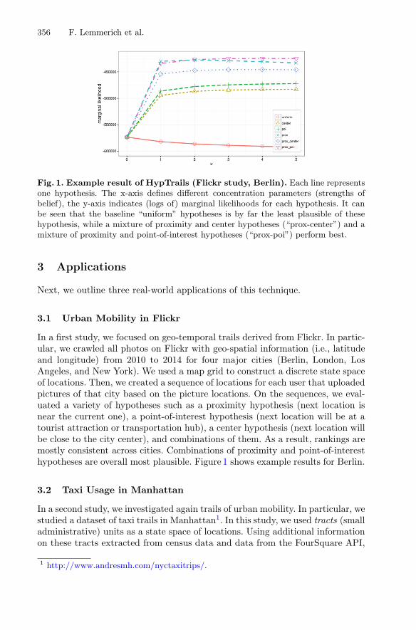
356 F. Lemmerich et al.
Fig. 1. Example result of HypTrails (Flickr study, Berlin). Each line representsone hypothesis. The x-axis defines different concentration parameters (strengths ofbelief), the y-axis indicates (logs of) marginal likelihoods for each hypothesis. It canbe seen that the baseline “uniform” hypotheses is by far the least plausible of thesehypothesis, while a mixture of proximity and center hypotheses (“prox-center”) and amixture of proximity and point-of-interest hypotheses (“prox-poi”) perform best.
3 Applications
Next, we outline three real-world applications of this technique.
3.1 Urban Mobility in Flickr
In a first study, we focused on geo-temporal trails derived from Flickr. In partic-ular, we crawled all photos on Flickr with geo-spatial information (i.e., latitudeand longitude) from 2010 to 2014 for four major cities (Berlin, London, LosAngeles, and New York). We used a map grid to construct a discrete state spaceof locations. Then, we created a sequence of locations for each user that uploadedpictures of that city based on the picture locations. On the sequences, we eval-uated a variety of hypotheses such as a proximity hypothesis (next location isnear the current one), a point-of-interest hypothesis (next location will be at atourist attraction or transportation hub), a center hypothesis (next location willbe close to the city center), and combinations of them. As a result, rankings aremostly consistent across cities. Combinations of proximity and point-of-interesthypotheses are overall most plausible. Figure 1 shows example results for Berlin.
3.2 Taxi Usage in Manhattan
In a second study, we investigated again trails of urban mobility. In particular, westudied a dataset of taxi trails in Manhattan1. In this study, we used tracts (smalladministrative) units as a state space of locations. Using additional informationon these tracts extracted from census data and data from the FourSquare API,
1 http://www.andresmh.com/nyctaxitrips/.
Comparing Hypotheses About Sequential Data 357
we investigated more than 60 hypotheses such as “taxis drive to tracts withsimilar ethnic distribution” or “taxis will drive to popular locations w.r.t. check-ins”. We also performed spatio-temporal clustering of the sequence data andapplied HypTrails on the individual clusters to find behavioral traits that aretypical for certain times and places. For instance, we discovered a group of taxirides to locations with a high density of party venues on weekend nights.
3.3 Link Usage in Wikipedia
In another work, we studied transitions between articles in the online encyclope-dia Wikipedia. In particular, we were interested in which links on a Wikipediapage get frequently used. For that purpose, we applied HypTrails on a recentlypublished dataset of all transitions between Wikipedia pages for one month2
using the set of all articles as state space. For constructing hypotheses, we con-sidered hypotheses based on visual features of the links (e.g., “links in the leadparagraph get clicked more often” or “links in the main text get clicked moreoften”), hypothesis based on text similarity between articles, and hypothesesbased on the structure of the link network of Wikipedia articles. As a result,hypotheses that assume people to prefer links at the top and left-hand side, andhypotheses that express a belief in more frequent usage of links towards theperiphery of the article network are most plausible.
4 Conclusion
In this work, we gave a short introduction into the HypTrails approach thatallows to compare the plausibility of hypotheses about the generation of a sequen-tial datasets. Additionally, we described three real-world applications of thistechnique for studying urban mobility and reading behavior in Wikipedia.
References
1. Becker, M., Singer, P., Lemmerich, F., Hotho, A., Helic, D., Strohmaier, M.: Pho-towalking the city: comparing hypotheses about urban photo trails on Flickr. In:International Conference on Social Informatics (SocInfo), pp. 227–244 (2015)
2. Dimitrov, D., Singer, P., Lemmerich, F., Strohmaier, M.: What makes a link suc-cessful on Wikipedia? In: International World Wide Web Conference, pp. 917–926(2017)
3. Espın Noboa, L., Lemmerich, F., Singer, P., Strohmaier, M.: Discovering and char-acterizing mobility patterns in urban spaces: a study of Manhattan taxi data. In:International Workshop on Location and the Web, pp. 537–542 (2016)
4. Kass, R.E., Raftery, A.E.: Bayes factors. J. Am. Stat. Assoc. 90(430), 773–795(1995)
5. Singer, P., Helic, D., Hotho, A., Strohmaier, M.: Hyptrails: a Bayesian approachfor comparing hypotheses about human trails on the web. In: International WorldWide Web Conference, pp. 1003–1013 (2015)
2 https://datahub.io/dataset/wikipedia-clickstream.
Data-Driven Approaches for Smart Parking
Fabian Bock1(B), Sergio Di Martino2, and Monika Sester1
1 Institute of Cartography and Geoinformatics, Leibniz University Hannover,Hannover, Germany
{bock,sester}@ikg.uni-hannover.de2 Department of Electrical Engineering and Information Technologies,
University of Naples “Federico II”, Naples, [email protected]
Abstract. Finding a parking space is a key problem in urban scenarios,often due to the lack of actual parking availability information for drivers.Modern vehicles, able to identify free parking spaces using standard on-board sensors, have been proven to be effective probes to measure parkingavailability. Nevertheless, spatio-temporal datasets resulting from probevehicles pose significant challenges to the machine learning and datamining communities, due to volume, noise, and heterogeneous spatio-temporal coverage. In this paper we summarize some of the approacheswe proposed to extract new knowledge from this data, with the final goalto reduce the parking search time. First, we present a spatio-temporalanalysis of the suitability of taxi movements for parking crowd-sensing.Second, we describe machine learning approaches to automatically gen-erate maps of parking spots and to predict parking availability. Finally,we discuss some open issues for the ML/KDD community.
1 Introduction
Very often, in urban scenarios, drivers have to roam at the end of their trips onthe search for a parking space, worsening the overall traffic and wasting time andfuel [5]. Smart Parking refers to Information and Communication Technologysolutions meant to improve parking search by providing information about park-ing locations and their actual or estimated availability. While it is rather trivialto gather parking availability information for parking facilities, it becomes trickyfor on-street parking, where there are mainly two sensing strategies: stationaryor mobile collection. The former relies on sensors embedded in the road infras-tructure, continuously measuring whether stalls are free or occupied. However, itis too expensive to cover a wider city area with those sensors. The latter mainlyexploits participatory or opportunistic crowd-sensing solutions from mobile appsor probe vehicles [6], that can occasionally detect free parking spaces. Mobilesensors are pretty cheap to deploy in comparison to the stationary ones butthe quality and the spatio-temporal resolution of the obtainable data streams islower, posing many challenges for the automatic extraction of useful knowledge.
In this paper, we give an overview of some approaches we used to exploitmobile sensor data for Smart Parking scenarios. In particular, in Sect. 2 wec© Springer International Publishing AG 2017Y. Altun et al. (Eds.): ECML PKDD 2017, Part III, LNAI 10536, pp. 358–362, 2017.https://doi.org/10.1007/978-3-319-71273-4_31
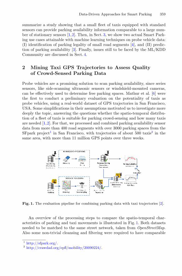
Data-Driven Approaches for Smart Parking 359
summarize a study showing that a small fleet of taxis equipped with standardsensors can provide parking availability information comparable to a large num-ber of stationary sensors [1,2]. Then, in Sect. 3, we show two actual Smart Park-ing use cases attainable with machine learning techniques on probe vehicle data:(I) identification of parking legality of small road segments [4], and (II) predic-tion of parking availability [3]. Finally, issues still to be faced by the ML/KDDCommunity are discussed in Sect. 4.
2 Mining Taxi GPS Trajectories to Assess Qualityof Crowd-Sensed Parking Data
Probe vehicles are a promising solution to scan parking availability, since seriessensors, like side-scanning ultrasonic sensors or windshield-mounted cameras,can be effectively used to determine free parking spaces. Mathur et al. [6] werethe first to conduct a preliminary evaluation on the potentiality of taxis asprobe vehicles, using a real-world dataset of GPS trajectories in San Francisco,USA. Some simplifications in their assumptions motivated us to investigate moredeeply the topic, answering the questions whether the spatio-temporal distribu-tion of a fleet of taxis is suitable for parking crowd-sensing and how many taxisare needed [1,2]. For that, we processed and combined parking availability sensordata from more than 400 road segments with over 3000 parking spaces from theSFpark project1 in San Francisco, with trajectories of about 500 taxis2 in thesame area, with more than 11 million GPS points over three weeks.
Fig. 1. The evaluation pipeline for combining parking data with taxi trajectories [2].
An overview of the processing steps to compare the spatio-temporal char-acteristics of parking and taxi movements is illustrated in Fig. 1. Both datasetsneeded to be matched to the same street network, taken from OpenStreetMap.Also some non-trivial cleansing and filtering were required to have comparable
1 http://sfpark.org/.2 http://crawdad.org/epfl/mobility/20090224/.
360 F. Bock et al.
datasets. The taxi trajectories were then aggregated to compute a typical weeklybehavior per road segment. Assuming that taxis would have observed parkingavailability each time they traversed a road segment, we calculated a dataset ofparking observations achievable by taxis by downsampling the stationary sensordata according to the timestamps of taxi visits per road segment. The actualparking availability was then estimated from the last observation of the taxis.
In a direct comparison of the parking availability information from mobileand stationary sensors, we found that the regular trips of 300 taxis (about 20%of all licensed taxis in San Francisco at that time) were sufficient to cover theSFpark project area in San Francisco with a maximal deviation of ±1 parkingspaces with respect to stationary sensors in more than 85% of the cases. Thisresult is remarkable since the taxi coverage revealed strong variability with thetime of day, but can be explained by the fact that parking turnover showeda similar time dependence. The time until the next taxi visit was less than30 min for about 60% of all road segments and time instants. Therefore, weconcluded that the spatio-temporal movements of taxis are well suited to crowd-sense parking availability.
3 Machine Learning Approaches for On-Street ParkingInformation
In this section we describe two use cases for Smart Parking we can derive on topof the data stream coming from probe vehicles.
Learning Parking Legality from Locations of Parked Vehicles. The location ofparking lanes and the legality of parking in a specific spot is the first relevantinformation for drivers looking for a free space. Parking might be not allowed infront of e.g. garage exits, or even for a full road if the road is narrow. Thus, driversshould focus their search on areas with many parking spaces. As the location ofparking spaces is often unknown to non-local drivers and on-street parking mapsdo not exist in many cities, we developed a crowd-sensing approach to learn theparking legality from the location of parked vehicles at different time instants [4].For every small road segment unit, several spatial and temporal features wereextracted and a binary decision was performed to distinguish legal from illegalparking spots. Multiple classifiers were evaluated on parking availability data,collected on 9 trips with a probe vehicle on more than five kilometers of potentialparking spaces. Results show that the random forest classifier achieved the bestresults. However, also k-means clustering plus a simple classification heuristicperformed nearly as good as the first one, without the need for costly trainingdata.
Predicting Parking Availability. Based on the parking availability information,a prediction is useful to provide a suggestion to drivers approaching their des-tination. There exist some data-driven prediction approaches in the literature[5], mostly formulated as a regression problem and only considering input data
Data-Driven Approaches for Smart Parking 361
at a constant frequency. Since most of the drivers are rather interested whetheror not there is at least one free parking space in a road segment and what isthe corresponding probability, we reformulated the problem as a binary classi-fication task that also is robust for irregular sampling [3]. As features, we usedthe last observations of the sensors in a road segment as well as the aggregatedobservations up to a certain distance in the surroundings, the parking capacity,and the time of day and day of week. We evaluated the approach using a randomforest classifier with data from the SFpark project. Results show that the binaryparking availability of a road segment can be predicted with a F1-score of about75% for 30 min ahead.
4 Conclusions and Open Issues
Crowd-sensing vehicles, measuring the on-street parking availability during theirregular trips, represent a new source for large amounts of parking data thatpromise to mitigate parking search problems. For example, maps of parkingspaces can be automatically generated, parking availability predicted, and searchrecommendations given to frustrated drivers. However, due to the highly irregu-lar spatio-temporal coverage of the generated data, also new research challengesarise for these applications. As the highly irregular sampling needs to be consid-ered, standard time series approaches cannot be applied to predict parking avail-ability. Also, as parking is a very dynamic phenomenon, extracting the trends inparking occupancy from the fluctuating data remains a challenge. Another openquestion is how learned models can be transferred to other cities. Finally, it isalso very relevant to investigate whether additional approaches are necessary forirregular events like concerts or sport matches.
References
1. Bock, F., Attanasio, Y., Di Martino, S.: Spatio-temporal road coverage of probevehicles: a case study on crowd-sensing of parking availability with taxis. In: Bregt,A., Sarjakoski, T., van Lammeren, R., Rip, F. (eds.) GIScience 2017. LNGC, pp.165–184. Springer, Cham (2017). https://doi.org/10.1007/978-3-319-56759-4 10
2. Bock, F., Di Martino, S.: How many probe vehicles do we need to collect on-streetparking information? In: 2017 International Conference on Models and Technologiesfor Intelligent Transportation Systems (MT-ITS). IEEE (2017)
3. Bock, F., Di Martino, S., Sester, M.: What are the potentialities of crowdsourcingfor dynamic maps of on-street parking spaces? In: Proceedings of the 9th ACMSIGSPATIAL International Workshop on Computational Transportation Science(IWCTS 2016), pp. 19–24. ACM, New York (2016)
4. Bock, F., Liu, J., Sester, M.: Learning on-street parking maps from position infor-mation of parked vehicles. In: Sarjakoski, T., Santos, M.Y., Sarjakoski, L.T. (eds.)Geospatial Data in a Changing World. LNGC, pp. 297–314. Springer, Cham (2016).https://doi.org/10.1007/978-3-319-33783-8 17

362 F. Bock et al.
5. Lin, T., Rivano, H., Moul, F.L.: A survey of smart parking solutions. IEEE Trans.Intell. Transp. Syst. PP(99), 1–25 (2017)
6. Mathur, S., Jin, T., Kasturirangan, N., Chandrasekaran, J., Xue, W., Gruteser,M., Trappe, W.: ParkNet: drive-by sensing of road-side parking statistics. In: Pro-ceedings of the 8th International Conference on Mobile Systems, Applications, andServices, pp. 123–136. ACM, New York (2010)
Image Representation, Annotation and Retrievalwith Predictive Clustering Trees
Ivica Dimitrovski1(B), Dragi Kocev2, Suzana Loskovska1, and Saso Dzeroski2
1 University of Ss Cyril and Methodius, Skopje, Macedonia{ivica.dimitrovski,suzana.loshkovska}@finki.ukim.mk
2 Jozef Stefan Institute, Ljubljana, Slovenia{Dragi.Kocev,Saso.Dzeroski}@ijs.si
Abstract. In this paper, we summarize our work on using the predictiveclustering framework for image analysis. More specifically, we have usedpredictive clustering trees to generate image representations, that canthen be used to perform image retrieval and/or image annotation. Wehave evaluated the proposed method for performing image retrieval ongeneral purpose images [6], and annotation of general purpose images[5], medical images [3] and diatom images [4].
Keywords: Image representation · Image retrievalImage annotation · Multi-target prediction · Predictive clustering
1 Introduction
The overwhelming increase in the amount of available visual information, espe-cially digital images, has brought up a pressing need to develop efficient andaccurate systems for image representation, retrieval and annotation. Most suchsystems for image analysis use the bag-of-visual-words representation of images.However, the computational bottleneck in all such systems is the construction ofthe visual codebook, i.e., obtaining the visual words. This is typically performedby clustering hundreds of thousands or millions of local descriptors, where theresulting clusters correspond to visual words. Each image is then represented bya histogram of the distribution of its local descriptors across the codebook.
The major issue in retrieval systems is that by increasing the sizes of theimage databases, the number of local descriptors to be clustered increasesrapidly: Thus, using conventional clustering techniques is infeasible. While exist-ing approaches are able to solve the efficiency issue, a part of the discriminativepower of the codebook is sacrificed for this. Considering this, we propose toconstruct the visual codebook by using predictive clustering trees (PCTs) [1],which can be constructed and executed efficiently and have good predictive per-formance.
PCTs are a generalization of decision trees towards the task of structuredoutput prediction, including multi-target regression, (hierarchical) multi-label
c© Springer International Publishing AG 2017Y. Altun et al. (Eds.): ECML PKDD 2017, Part III, LNAI 10536, pp. 363–367, 2017.https://doi.org/10.1007/978-3-319-71273-4_32

364 I. Dimitrovski et al.
classification and time series prediction. Moreover, the definition of descriptive,clustering and target attributes is flexible thus facilitating the learning of bothunsupervised and supervised trees. Furthermore, to increase the stability of themodel, we propose to use random forests of PCTs [7]. We create a randomforest of PCTs that represents the codebook, i.e., is used to generate the imagerepresentation.
The images represented with the bag-of-visual-words can then be used to per-form image retrieval and/or annotation. In the former, the indexing structurefor performing the retrieval is the same structure representing the codebook –the random forest of PCTs. We evaluate the proposed bag-of-visual-words app-roach for image retrieval on five benchmark reference datasets. The results revealthat the proposed method produces a visual codebook with superior discrimi-native power and thus better retrieval performance while maintaining excellentcomputational efficiency [6].
Additional complexity of image annotation arises from the complexity of thelabels used for annotation: Typically, an image depicts more than one object,hence more than one label should be assigned for that image. Moreover, theremight be some structure among the labels, such as a hierarchy of labels. Toaddress this additional complexity, we learn ensembles of PCTs to exploit thepotential relations that may exist among the labels. We have evaluated thisapproach on three tasks: multi-label classification of general purpose images [5],and hierarchical multi-label classification of medical images [3], as well as diatomimages [4]. The results of the evaluation show that we achieve state-of-the-artpredictive performance.
The remainder of this paper is organized as follows. We next briefly presentthe predictive clustering framework. We then outline the method for constructingimage representations. Finally, we describe the evaluation of this approach, firstfor image retrieval and then for image annotation.
2 Predictive Clustering Framework
Predictive Clustering Trees (PCTs) [1] generalize decision trees and can be usedfor a variety of learning tasks including different types of prediction and clus-tering. The PCT framework views a decision tree as a hierarchy of clusters: thetop-node of a PCT corresponds to one cluster containing all data, which is recur-sively partitioned into smaller clusters while moving down the tree. The leavesrepresent the clusters at the lowest level of the hierarchy and each leaf is labeledwith its cluster’s prototype (prediction). One of the most important steps in thePCT algorithm is the test selection procedure. For each node, a test is selectedby using a heuristic function computed on the training examples. The heuris-tic used in this algorithm for selecting the attribute tests in the internal nodesis the reduction in variance caused by partitioning the instances. Maximizingthe variance reduction maximizes cluster homogeneity and improves predictiveperformance.
Image Representation, Annotation and Retrieval 365
In this work, we used three instantiations of PCTs for the tasks of multi-target regression (MTR), multi-label classification (MLC) and hierarchical multi-label classification (HMC). For the MTR task, the variance is calculated as thesum of the normalized variances of the target variables. For the MLC task, weused the sum of the Gini indices of the labels, while for the HMC task, thevariance is calculated by using a weighted Euclidean distance that considers thehierarchy of the labels. The prototype function returns as a prediction the tuplewith the mean values of the target variables, calculated by using the traininginstances that belong to the given leaf.
3 PCTs for Image Representation
The proposed method for constructing the visual codebook is as follows. First,we randomly select a subset of the local (SIFT) descriptors from all of the train-ing images [8]. Next, the selected local descriptors constitute the training setused to construct a PCT. For the construction of a PCT, we set the descriptiveattributes (i.e., the 128 dimensional vector of the local descriptor) to be also tar-get and clustering attributes. Note that this feature is a unique characteristic ofthe predictive clustering framework. The PCTs are computationally efficient: itis very fast to both construct them and use them to make predictions. However,tree learning is unstable, i.e., the structure of the learned tree can change sub-stantially for small changes in the training data [2]. To overcome this limitationand to further improve the discriminative power of the indexing structure, weuse an ensemble (i.e., random forest) of PCTs. The overall codebook is obtainedby concatenating the codebooks from each tree.
4 PCTs for Image Retrieval
In the proposed system, a PCT (or a random forest of PCTs) representsthe search/indexing structure used to retrieve images similar to query images.Namely, for each image descriptor (i.e., each training example used to constructthe PCTs), we keep a unique index/identifier. The identifier consists of the imageID from which the local descriptor was extracted coupled with a descriptor ID.This indexing allows for faster computation of the image similarities.
We have evaluated the proposed improvement of the bag-of-visual words app-roach on three reference datasets and two additional datasets of 100 K imagesand 1 M images, comparing it to two state-of-the-art methods based on approx-imate k-means and extremely randomized tree ensembles. The results from theexperimental evaluation reveal the following. First and foremost, our systemexhibits better retrieval performance by 6–8% (mean average precision) thanboth competing methods at the same efficiency. Additionally, the increase of thenumber of local descriptors and number of PCTs used to create the indexingstructure improve the retrieval performance of the system.

366 I. Dimitrovski et al.
5 PCTs for Hierarchical Annotation of Images
We first use our system for multi-label annotation of general purpose images[5]. We compare the efficiency and the discriminative power of the proposedapproach to the literature standard of using k-means clustering. The resultsreveal that our approach is much more efficient in terms of computational time(24.4 times faster) and produces a visual codebook with better discriminativepower as compared to k-means clustering. Moreover, the difference in predictiveperformance increases with the average number of labels per image.
Next, we evaluate the performance of ensembles of PCTs for HMC (bag-ging and random forests) on the task of annotation of medical images using thehierarchy from the DICOM header [3]. The experiments on the IRMA databaseshow that random forests of PCTs for HMC outperform SVMs for flat classifica-tion. The average difference is 17 points for the ImageCLEF2007 and 20 pointsfor the ImageCLEF2008 dataset (a point in the hierarchical evaluation measureroughly corresponds to one completely misclassified image). Additionally, therandom forests are the fastest method; they are 10 times faster than baggingand 5.5 times faster than the SVMs.
Finally, for the task of hierarchical annotation of diatom images, by usingrandom forests of PCTs for HMC, we obtained the best results on the differentvariants of the ADIAC database of diatom images [4]: The obtained predictivepower of our method was in the range 96–98%. More specifically, we outper-formed a variety of methods for annotation that use SVMs, bagged decision treesand neural networks. Finally, we used these annotations in an on-line annotationsystem to assist taxonomists in identifying a wide range of different diatoms.
Acknowledgments. We would like to acknowledge the support of the European Com-mission through the project MAESTRA - Learning from Massive, Incompletely anno-tated, and Structured Data (Grant number ICT-2013-612944).
References
1. Blockeel, H., Raedt, L.D., Ramon, J.: Top-down induction of clustering trees. In:Proceedings of the 15th International Conference on Machine Learning, pp. 55–63.Morgan Kaufmann (1998)
2. Breiman, L.: Random forests. Mach. Learn. 45(1), 5–32 (2001)3. Dimitrovski, I., Kocev, D., Loskovska, S., Dzeroski, S.: Hierarchical annotation of
medical images. Pattern Recognit. 44(10–11), 2436–2449 (2011)4. Dimitrovski, I., Kocev, D., Loskovska, S., Dzeroski, S.: Hierarchical classification
of diatom images using ensembles of predictive clustering trees. Ecol. Inform. 7(1),19–29 (2012)
5. Dimitrovski, I., Kocev, D., Loskovska, S., Dzeroski, S.: Fast and efficient visualcodebook construction for multi-label annotation using predictive clustering trees.Pattern Recognit. Lett. 38, 38–45 (2014)
6. Dimitrovski, I., Kocev, D., Loskovska, S., Dzeroski, S.: Improving bag-of-visual-words image retrieval with predictive clustering trees. Inf. Sci. 329, 851–865 (2016)

Image Representation, Annotation and Retrieval 367
7. Kocev, D., Vens, C., Struyf, J., Dzeroski, S.: Tree ensembles for predicting structuredoutputs. Pattern Recognit. 46(3), 817–833 (2013)
8. Lowe, D.G.: Distinctive image features from scale-invariant keypoints. Int. J. Com-put. Vis. 60(2), 91–110 (2004)

Music Generation Using Bayesian Networks
Tetsuro Kitahara(B)
College of Humanities and Sciences, Nihon University,3-25-40, Sakurajosui, Stagaya-ku, Tokyo 156-8550, Japan
http://www.kthrlab.jp/
Abstract. Music generation has recently become popular as an appli-cation of machine learning. To generate polyphonic music, one must con-sider both simultaneity (the vertical consistency) and sequentiality (thehorizontal consistency). Bayesian networks are suitable to model bothsimultaneity and sequentiality simultaneously. Here, we present musicgeneration models based on Bayesian networks applied to chord voicing,four-part harmonization, and real-time chord prediction.
1 Introduction
Music is widely known as an application domain of machine learning. However,in the beginning of the 21st century, recognition/analysis tasks were activelystudied, such as music transcription and genre classification. But recently, thenumber of studies devoted to music generation has been increasing (e.g., [1]).
When generating polyphonic music, one must consider two-directional con-sistencies: simultaneity (i.e., the vertical or pitch-axis consistency) and sequen-tiality (i.e., the horizontal or time-axis consistency). Our team has investigatedmusic generation models considering both simultaneity and sequentiality usingBayesian networks [2–4]. Here, we present our models applied to chord voicing [2],four-part harmonization [3], and real-time chord prediction [4].
2 Assumed Music Structure and Fundamental Model
Suppose that a chord progression C = [c1, c2, · · ·, cN ] (ci: chord symbol) existsin a piece of music. Each chord ci (e.g., Am) is played with a particularvoicing (a(1)i , a
(2)i , · · ·, a(K)
i ) (a(k)i : note name (a.k.a. pitch class)) (e.g., (C,E, A)). As noted in Introduction, a set of simultaneous notes (a(1)i , a
(2)i , · · ·, a(K)
i )should be harmonically consistent with one other, and each sequence A(k) =[a(k)1 , a
(k)2 , · · ·, akN ] should be temporally smooth. At the same time, a melody
M = [m1,1,m1,2, · · ·,m2,1, · · · ] exists, where mi,j represents the note name ofthe j-th note in the i-th chord region. The sequences of chords, voicings, and
This work was supported by JSPS KAKENHI Grant Numbers 16K16180, 16H01744,16KT0136, and 17H00749.
c© Springer International Publishing AG 2017Y. Altun et al. (Eds.): ECML PKDD 2017, Part III, LNAI 10536, pp. 368–372, 2017.https://doi.org/10.1007/978-3-319-71273-4_33
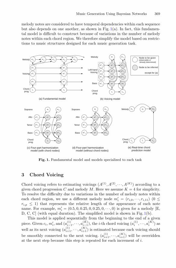
Music Generation Using Bayesian Networks 369
melody notes are considered to have temporal dependencies within each sequencebut also depends on one another, as shown in Fig. 1(a). In fact, this fundamen-tal model is difficult to construct because of variations in the number of melodynotes within each chord region. We therefore simplify the model based on restric-tions to music structures designed for each music generation task.
Fig. 1. Fundamental model and models specialized to each task
3 Chord Voicing
Chord voicing refers to estimating voicings (A(1), A(2), · · ·, A(K)) according to agiven chord progression C and melody M . Here we assume K = 4 for simplicity.To resolve the difficulty due to variations in the number of melody notes withineach chord region, we use a different melody node m′
i = (ri,0, · · ·, ri,11) (0 ≤ri,p ≤ 1) that represents the relative length of the appearance of each notename. For example, m′
i = (0.5, 0, 0.25, 0, 0.25, 0, · · ·, 0) is given for a melody [E,D, C, C] (with equal duration). The simplified model is shown in Fig. 1(b).
This model is applied sequentially from the beginning to the end of a givenpiece. Given ci, m′
i, and (a(1)i−1, · · ·, a(K)i−1), the i-th chord voicing (a(1)i , · · ·, a(K)
i ) aswell as its next voicing (a(1)i+1, · · ·, a(K)
i+1) is estimated because each voicing shouldbe smoothly connected to the next voicing. (a(1)i+1, · · ·, a(K)
i+1) will be overriddenat the next step because this step is repeated for each increment of i.

370 T. Kitahara
An example of chord voicing is shown in Fig. 2. The model has been trainedwith 30 jazz pieces arranged for the electronic organ. Listening tests conductedby music experts revealed that 94.7% of the chord voicings were acceptable.
Fig. 2. An example of voicing (excerpted)
4 Four-Part Harmonization
Here, we focus on harmonization. Unlike voicing, a sequence of chord symbols isnot given—it has to be estimated. For simplicity, we adopt the “one chord for onemelody note” assumption. Based on this assumption, the Bayesian network canbe simplified to that shown in Fig. 1(c). Here we assume K = 3. This problem iscalled four-part harmonization because the harmony consists of four voices (i.e.,soprano, alto, tenor, and bass). Furthermore, we constructed a Bayesian networkin which the chord nodes are removed (Fig. 1(d)) because the chord symbols aresometimes too ambiguous.
Fig. 3. Example of harmonization (left: model with chord nodes, right: model withoutchord nodes)
Figure 3 shows an example of harmonization using these two models. Ourobjective quantitative evaluation reveals that the model shown in Fig. 1(d) gen-erates more temporally smooth harmonies than the model shown in Fig. 1(c)even though harmonizations with the former model tend to contain slightly moredissonant sounds.
5 Real-Time Chord Prediction
Finally, we apply our Bayesian network to real-time chord prediction. Musicexperts can often precisely predict the next chord by listening to the currentchord, even if they are not familiar with the piece being played. This ability
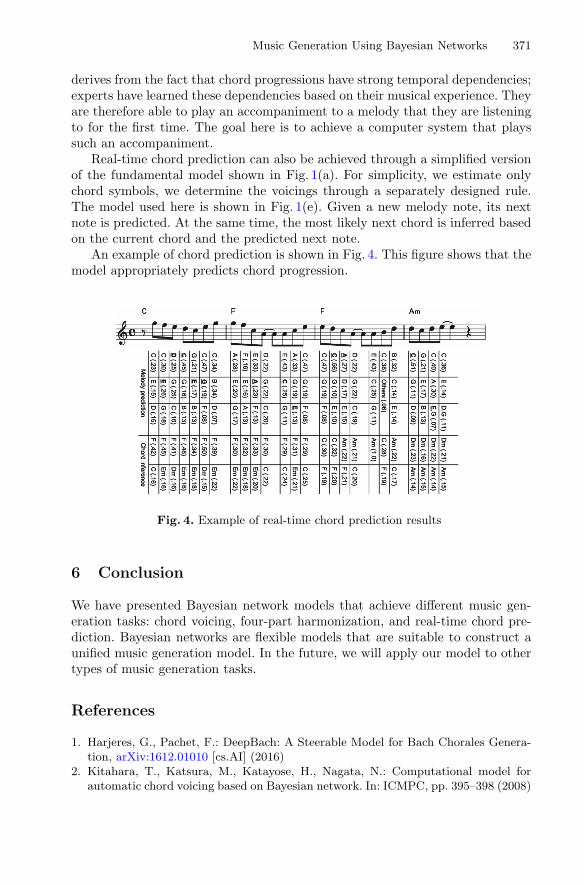
Music Generation Using Bayesian Networks 371
derives from the fact that chord progressions have strong temporal dependencies;experts have learned these dependencies based on their musical experience. Theyare therefore able to play an accompaniment to a melody that they are listeningto for the first time. The goal here is to achieve a computer system that playssuch an accompaniment.
Real-time chord prediction can also be achieved through a simplified versionof the fundamental model shown in Fig. 1(a). For simplicity, we estimate onlychord symbols, we determine the voicings through a separately designed rule.The model used here is shown in Fig. 1(e). Given a new melody note, its nextnote is predicted. At the same time, the most likely next chord is inferred basedon the current chord and the predicted next note.
An example of chord prediction is shown in Fig. 4. This figure shows that themodel appropriately predicts chord progression.
Fig. 4. Example of real-time chord prediction results
6 Conclusion
We have presented Bayesian network models that achieve different music gen-eration tasks: chord voicing, four-part harmonization, and real-time chord pre-diction. Bayesian networks are flexible models that are suitable to construct aunified music generation model. In the future, we will apply our model to othertypes of music generation tasks.
References
1. Harjeres, G., Pachet, F.: DeepBach: A Steerable Model for Bach Chorales Genera-tion, arXiv:1612.01010 [cs.AI] (2016)
2. Kitahara, T., Katsura, M., Katayose, H., Nagata, N.: Computational model forautomatic chord voicing based on Bayesian network. In: ICMPC, pp. 395–398 (2008)

372 T. Kitahara
3. Suzuki, S., Kitahara, T.: Four-part harmonization using Bayesian networks: prosand cons of introducing chord nodes. J. New Music Res. 43(3), 331–353 (2014)
4. Kitahara, T., Totani, N., Tokuami, R., Katayose, H.: BayesianBand: jam session sys-tem based on mutual prediction by user and system. In: Natkin, S., Dupire, J. (eds.)ICEC 2009. LNCS, vol. 5709, pp. 179–184. Springer, Heidelberg (2009). https://doi.org/10.1007/978-3-642-04052-8 17

Phenotype Inference from Textand Genomic Data
Maria Brbić1, Matija Piškorec1, Vedrana Vidulin1, Anita Kriško2,Tomislav Šmuc1, and Fran Supek1,3(B)
1 Ruđer Bošković Institute, Zagreb, Croatia2 Mediterranean Institute of Life Sciences, Split, Croatia
3 Centre for Genomic Regulation, Barcelona, [email protected]
Abstract. We describe ProTraits, a machine learning pipeline that sys-tematically annotates microbes with phenotypes using a large amount oftextual data from scientific literature and other online resources, as wellas genome sequencing data. Moreover, by relying on a multi-view non-negative matrix factorization approach, ProTraits pipeline is also able todiscover novel phenotypic concepts from unstructured text. We presentthe main components of the developed pipeline and outline challengesfor the application to other fields.
Keywords: Phenotypic trait · Microbes · Comparative genomicsLate fusion · Text mining · Non-negative matrix factorization
1 Introduction
With the development of next-generation DNA sequencing techniques, the num-ber of available microbial genomes has rapidly increased. However, this explosivegrowth of genomics data is not followed by the phenotypic annotations of organ-isms, such as growth at extreme temperatures, resistance to radiation, or theability to cause disease in plants, animals or humans. The systematic annota-tion of organisms with phenotypic traits is of importance for discovering theassociations between genes to phenotypes that would suggest a biological basisfor various traits. Existing databases [7,11] rely on manual annotation of organ-isms, which results in limited coverage. On the other hand, there is a vast amountof unstructured data with phenotype descriptions available in scientific articlesand other textual resources. Motivated by this abundance of genomic and of tex-tual data, we developed ProTraits [2] - a machine learning-based pipeline thatsystematically assigns predictions across large number of organisms and phe-notypes. Along with predicting existing phenotypic labels, ProTraits pipelineis also able to define novel phenotypic concepts from unstructured text usinga multi-view approach based on non-negative matrix factorization followed byclustering and manual curation. Here, we briefly describe main components of
c© Springer International Publishing AG 2017Y. Altun et al. (Eds.): ECML PKDD 2017, Part III, LNAI 10536, pp. 373–377, 2017.https://doi.org/10.1007/978-3-319-71273-4_34
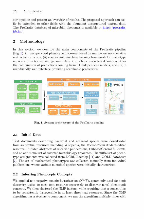
374 M. Brbić et al.
our pipeline and present an overview of results. The proposed approach can eas-ily be extended to other fields with the abundant unstructured textual data.The ProTraits database of microbial phenomes is available at http://protraits.irb.hr/.
2 Methodology
In this section, we describe the main components of the ProTraits pipeline(Fig. 1): (i) unsupervised phenotype discovery based on multi-view non-negativematrix factorization; (ii) a supervised machine learning framework for phenotypeinference from textual and genomic data; (iii) a late-fusion based component forthe combination of predictions coming from 11 independent models, and (iv) auser-friendly web interface providing searchable predictions.
Fig. 1. System architecture of the ProTraits pipeline
2.1 Initial Data
Text documents describing bacterial and archaeal species were downloadedfrom six textual resources including Wikipedia, the MicrobeWiki student-editedresource, PubMed abstracts of scientific publications, PubMedCentral full-texts,and an additional set of assorted microbiology resources. The initial set of pheno-type assignments was collected from NCBI, BacMap [11] and GOLD databases[7]. The set of biochemical phenotypes was collected manually from individualpublications where various microbial species were initially characterized.
2.2 Inferring Phenotypic Concepts
We applied non-negative matrix factorization (NMF), commonly used for topicdiscovery tasks, to each text resource separately to discover novel phenotypicconcepts. We then clustered the NMF factors, while requiring that a concept hasto be consistently discoverable in at least three text resources. Since the NMFalgorithm has a stochastic component, we ran the algorithm multiple times with
Phenotype Inference from Text and Genomic Data 375
different random seeds while also varying the number of factors parameter, inorder to maximize the diversity of discovered concepts. These groups were thenexamined by an expert and those describing new phenotypes were retained andused in the same way as labels collected from the existing databases. In total,we discovered 113 non-redundant novel phenotypic concepts.
2.3 Phenotype Prediction
In the phenotype prediction task, the learning examples were species and theclass label was the presence/absence of a phenotype in that species. A separatemodel was trained for each of the 424 phenotypes and 10-fold cross-validationused to estimate the accuracy. Once a model was learned, it was applied to thespecies with unknown phenotypic annotations. To make the functioning of ourmodels more interpretable to biologists, we also provide sets of most importantfeatures of all models.
Predictions from textual data. We used bag-of-words representation with tf-idf weighting of word frequencies across documents assigned to species in a giventext corpus. A Support vector machine (SVM) classifier with a linear kernel wastrained on all combinations of text resources and phenotypes.
Predictions from genome data. We constructed five different genomic repre-sentations for each microbial species: (i) the proteome composition [1,9]; (ii) thegene repertoire encoded as presence/absence of Clusters of Orthologous Groups(COG) gene families [4,6]; (iii) co-occurrence of species across environmentalsequencing data sets [3]; (iv) gene neighborhoods [8] encoded as pairwise chro-mosomal distances between gene family members; and (v) genomic signaturesof translation efficiency in gene families [5,10]. Again, we trained models on allcombinations of representations and phenotypes. We used the Random Forest(RF) classifier which we found to outperform other tested algorithms.
Combining predictions. To combine predictions from different models andprovide an interpretable estimate of confidence in each prediction, the confidencescores of each prediction were converted to precisions, based on cross-validationprecision-recall curves. Precision scores for organisms in the initially unlabeledset of organisms were calculated via linear interpolation between the neighboringconfidence points and then assigned to both positive and negative class for eachprediction and further adjusted to account for difference in class sizes, ensuringthat the minimum precision of each class is 0, regardless of the number of posi-tive/negative examples. The systematic validation performed by two experts ona random sample of 2, 500 predictions showed that the precisions combined usinglate fusion schemes agree well with human judgment, particularly when requiringagreement of two independent models (either text or genomics-derived).
Web interface and results. In summary, ProTraits covers 3, 046 microbialorganisms and 424 microbial phenotypes. It provides predictions across six tex-tual resources and five independent genomic representations. At the precision

376 M. Brbić et al.
threshold higher than 0.9, ProTraits assigns ≈545,000 novel annotations, out ofwhich ≈308,000 are supported in two or more independent predictions. A webinterface at http://protraits.irb.hr/ provides precision scores across 11 individ-ual predictors and an integrated score calculated using the two-votes late fusionscheme.
3 Challenges and Conclusions
Training separate classifiers for each of the phenotypes does not scale well interms of computation time required, especially for high-dimensional genomicdatasets. However, using existing multi-label classifiers was not straightforwardfor our datasets since most of the target values were missing. Another challengewas collecting initial labels, as this requires tedious manual curation. While thetwo existing microbial phenotype databases alleviated this problem in our work,for other important problems in the life sciences, similar databases may not beavailable. Crucially, the input of field experts has allowed us to validate predic-tions and inferred concepts, demonstrating that our models are trustworthy.
Acknowledgments. This work has been funded by the by the European Union FP7grants ICT-2013-612944 (MAESTRA) and Croatian Science Foundation grants HRZZ-9623.
References
1. Brbić, M., Warnecke, T., Kriško, A., Supek, F.: Global shifts in genome and pro-teome composition are very tightly coupled. Genome Biol. Evol. 7, 1519–1532(2015)
2. Brbić, M., Piškorec, M., Vidulin, V., Kriško, A., Šmuc, T., Supek, F.: The landscapeof microbial phenotypic traits and associated genes. Nucleic Acids Res. 44, 10074–10090 (2016)
3. Chaffron, S., Rehrauer, H., Pernthaler, J., von Mering, C.: A global network ofcoexisting microbes from environmental and whole-genome sequence data. GenomeRes. 20, 947–959 (2010)
4. Feldbauer, R., Schulz, F., Horn, M., Rattei, T.: Prediction of microbial phenotypesbased on comparative genomics. BMC Bioinform. 16, 1–8 (2015)
5. Kriško, A., Copić, T., Gabaldón, T., Lehner, B., Supek, F.: Inferring gene functionfrom evolutionary change in signatures of translation efficiency. Genome Biol. 15,R44 (2014)
6. MacDonald, N.J., Beiko, R.G.: Efficient learning of microbial genotype-phenotypeassociation rules. Bioinformatics 26, 1834–1840 (2010)
7. Reddy, T.B.K., Thomas, A.D., Stamatis, D., Bertsch, J., Isbandi, M., Jansson, J.,Mallajosyula, J., Pagani, I., Lobos, E.A., Kyrpides, N.C.: The Genomes OnLineDatabase (GOLD) v. 5: a metadata management system based on a four level(meta)genome project classification. Nucleic Acids Res. 43, D1099–1106 (2015)
8. Rogozin, I.B., Makarova, K.S., Murvai, J., Czabarka, E., Wolf, Y.I., Tatusov,R.L., Szekely, L.A., Koonin, E.V.: Connected gene neighborhoods in prokaryoticgenomes. Nucleic Acids Res. 30, 2212–2223 (2002)

Phenotype Inference from Text and Genomic Data 377
9. Smole, Z., Nikolic, N., Supek, F., Šmuc, T., Sbalzarini, I.F., Kriško, A.: Proteomesequence features carry signatures of the environmental niche of prokaryotes. BMCEvol. Biol. 11–26 (2011)
10. Supek, F., Škunca, N., Repar, J., Vlahoviček, K., Šmuc, T.: Translational selectionis ubiquitous in prokaryotes. PLoS Genet. 6, e1001004 (2010)
11. Stothard, P., Van Domselaar, G., Shrivastava, S., Guo, A., O’Neill, B., Cruz, J.,Ellison, M., Wishart, D.S.: BacMap: an interactive picture atlas of annotated bac-terial genomes. Nucleic Acids Res. 33, D317–D320 (2005)
Process-Based Modeling and Designof Dynamical Systems
Jovan Tanevski1(B), Nikola Simidjievski1, Ljupco Todorovski1,2,and Saso Dzeroski1
1 Jozef Stefan Institute, Ljubljana, Slovenia{jovan.tanevski,nikola.simidjievski,saso.dzeroski}@ijs.si
2 University of Ljubljana, Ljubljana, [email protected]
Abstract. Process-based modeling is an approach to constructingexplanatory models of dynamical systems from knowledge and data. Theknowledge encodes information about potential processes that explainthe relationships between the observed system entities. The resultingprocess-based models provide both an explanatory overview of the sys-tem components and closed-form equations that allow for simulatingthe system behavior. In this paper, we present three recent improve-ments of the process-based approach: (i) improving predictive perfor-mance of process-based models using ensembles, (ii) extending the scopeof process-based models towards handling uncertainty and (iii) address-ing the task of automated process-based design.
1 Introduction
Process-based modeling (PBM) supports knowledge discovery by learning under-standable and communicable models of dynamical systems. PBM uses domain-specific knowledge as declarative bias in combination with observed time-seriesdata to address the task of modeling real-world systems. It performs both struc-ture identification and parameter estimation, resulting in a process-based modelwhich specifies a set of differential equations. In turn, such models accuratelycapture the complex and nonlinear behavior of a dynamical system through time.
Learning models of dynamical systems is a supervised machine learning task:the predictive variables correspond to observed system variables, while the tar-gets correspond to their time derivatives. However, the task bears two specificproperties that limit the use of traditional machine learning approaches. First,the resulting models take the form of a set of entities, processes and differentialequations, i.e., artifacts used by scientists and engineers to construct explana-tory models. On the other hand, machine learning methods operate on classesof predictive models that generalize well over arbitrary data, while keeping thecomplexity of training and evaluation procedures low. Second, the observed vari-ables are measured at consecutive time points, so the data instances breach thecommon assumption of their mutual independence.c© Springer International Publishing AG 2017Y. Altun et al. (Eds.): ECML PKDD 2017, Part III, LNAI 10536, pp. 378–382, 2017.https://doi.org/10.1007/978-3-319-71273-4_35
Process-Based Modeling and Design of Dynamical Systems 379
The PBM approach relies on the paradigm of computational scientificdiscovery [3] and more specifically, on approaches to inductive process modeling.On one hand, research in this area has a long tradition and has been applied toa variety of domains [1,2,10,11]. However, while successful, it has been at themargins of mainstream machine learning. On the other hand, the PBM approachhas so far focused primarily on applications within a narrow class of problemsthat emphasize descriptive and deterministic models at output, given a singledata type at input. In terms of output, such models are typically simulated andanalyzed using the learning data. Therefore, they have a tendency to overfit– rendering them incapable at accurately predicting future system’s behavior.Also, these models do not capture the intrinsic uncertainty of the interactionsin the system. They always predict exactly the same behavior of the systemat output in a deterministic manner: determined only by initial conditions andignoring the uncertainty in real-world systems. In terms of input, an assumptionof the PBM is that time-series of observations are always available and sufficient.This, however, does not hold for problems with limited observability or tasks,such as design, where different types of input are required.
In response, our recent developments of the PBM approach have aimed atbridging the gap between machine learning and domains of application withinphysical and life sciences. We address the limitations of the PBM approachby broadening the classes of tasks it can address. We build on the traditionof constant performance improvement, but also extend the scope of potentialapplications. In particular, to improve the performance on the task of predictivemodeling, we support the learning of different types of ensembles of process-basedmodels [4–6]. Next, we extended the output to include process-based models thatdescribe stochastic interactions [7]. Finally, in order to address tasks of modelingdynamical systems under limited observability and tasks of design of dynamicalsystems, we consider different types of input data. Namely, in addition to time-series of observations of system variables we allow for the definition of expectedproperties of the behavior of the dynamical system [8,9].
2 Methods
The PBM learning task takes domain-specific knowledge and time-series dataat input (Fig. 1). The resulting model comprises system variables represented asentities and their interactions that define the underlying model structure rep-resented as processes. This representation allows for straightforward mapping ofprocess-based models into a set of differential equations. The model parametersare fitted to the data using evolutionary optimization methods with the sum-of-squares loss function as the objective. The PBM approach, however, adds anextra layer to the model equations. In particular, the models are constructedusing components from a library of domain-knowledge, represented by templateentities and processes. These templates encode taxonomies of variable and con-stant properties of the constituents in the dynamical systems as well as the tax-onomies of processes (interactions) among them. The (partial) instantiations of
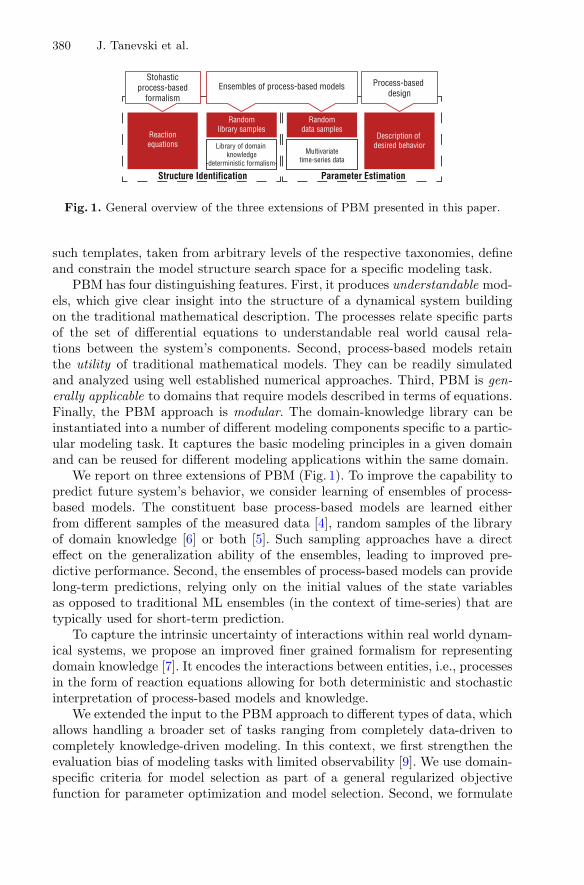
380 J. Tanevski et al.
Structure Identification Parameter Estimation
Library of domain knowledge
-deterministic formalism-
Reactionequations
Randomlibrary samples
Randomdata samples
Multivariatetime-series data
Description of desired behavior
Stohastic process-based
formalismEnsembles of process-based models Process-based
design
Fig. 1. General overview of the three extensions of PBM presented in this paper.
such templates, taken from arbitrary levels of the respective taxonomies, defineand constrain the model structure search space for a specific modeling task.
PBM has four distinguishing features. First, it produces understandable mod-els, which give clear insight into the structure of a dynamical system buildingon the traditional mathematical description. The processes relate specific partsof the set of differential equations to understandable real world causal rela-tions between the system’s components. Second, process-based models retainthe utility of traditional mathematical models. They can be readily simulatedand analyzed using well established numerical approaches. Third, PBM is gen-erally applicable to domains that require models described in terms of equations.Finally, the PBM approach is modular. The domain-knowledge library can beinstantiated into a number of different modeling components specific to a partic-ular modeling task. It captures the basic modeling principles in a given domainand can be reused for different modeling applications within the same domain.
We report on three extensions of PBM (Fig. 1). To improve the capability topredict future system’s behavior, we consider learning of ensembles of process-based models. The constituent base process-based models are learned eitherfrom different samples of the measured data [4], random samples of the libraryof domain knowledge [6] or both [5]. Such sampling approaches have a directeffect on the generalization ability of the ensembles, leading to improved pre-dictive performance. Second, the ensembles of process-based models can providelong-term predictions, relying only on the initial values of the state variablesas opposed to traditional ML ensembles (in the context of time-series) that aretypically used for short-term prediction.
To capture the intrinsic uncertainty of interactions within real world dynam-ical systems, we propose an improved finer grained formalism for representingdomain knowledge [7]. It encodes the interactions between entities, i.e., processesin the form of reaction equations allowing for both deterministic and stochasticinterpretation of process-based models and knowledge.
We extended the input to the PBM approach to different types of data, whichallows handling a broader set of tasks ranging from completely data-driven tocompletely knowledge-driven modeling. In this context, we first strengthen theevaluation bias of modeling tasks with limited observability [9]. We use domain-specific criteria for model selection as part of a general regularized objectivefunction for parameter optimization and model selection. Second, we formulate

Process-Based Modeling and Design of Dynamical Systems 381
the novel task of process-based design of dynamical systems [8]. This approachdoes not take measured data at input, but is completely based on the descriptionof desired properties of the behavior of a dynamical system. We further gener-alize the task by taking advantage of methods for simultaneous optimization ofmultiple conflicting objectives (desired properties of the behavior). We use thecomplete information from the Pareto front of optimal solutions (obtained forevery candidate design) to rank the designs and make a well informed selection.
3 Significance and Challenges
The methodology for learning ensembles of PBMs extends the scope of thetraditional ensemble paradigm in machine learning towards modeling dynam-ical systems. It improves the generalization power of PBMs, providing moreaccurate simulation of the future behavior of the modeled systems. The pro-posed methodology employs four different methods for constructing ensemblesof process-based models. Each of these significantly improves the predictive per-formance (on average up to 60% of relative improvement) over individual modelson tasks of modeling population dynamics in three lake ecosystems [4–6].
The extension of the PBM approach towards stochastic process-based mod-els has allowed us to model dynamical systems that are out of the scope ofdeterministic models. We have demonstrated that the stochastic PBM is capa-ble of reconstructing known, manually constructed models from synthetic andreal-world data in the domains of systems biology and epidemiology [7].
The capability of PBM to handle different inputs and multiple model-ing objectives has led to important contributions in the domains of systemsand synthetic biology. In particular, PBM can address the problem of highstructural uncertainty (many candidate model structures) and incomplete data(i.e., limited observability of the system variables). In system biology, our app-roach can alleviate the model selection problem by strengthening the evaluationbias with introducing domain-specific model selection criteria [9]. In syntheticbiology, we can now use PBM to solve the task of automated design. Our resultsshow that PBM is capable of reconstructing known/good designs, as well asproposing novel alternative designs of a synthetic stochastic switch and a syn-thetic oscillator [8].
Note, finally, that all three extensions of the PBM approach are designed andimplemented as independent modular components. Therefore, they are interop-erable. They can be, in principle, arbitrarily combined and applied to novel tasks,such as learning ensembles of stochastic process-based models.
Several challenges, that we are aware of and currently working on, remain inPBM. The exhaustive combinatorial search currently in use is computationallyinefficient and does not scale well with the number of candidate model struc-tures. It is therefore necessary to integrate methods for heuristic search in ourcurrent implementation. An alternative approach to reducing search complexityis to use higher-level constraints on model structures that are more expressivethan the current constraints. They can be based on the topological properties

382 J. Tanevski et al.
of the candidate model structures, or can define a probability distribution overthe model structures. Finally, both process-based modeling and design requirefurther evaluation on other related domains, such as neurobiology, systems phar-macology and systems medicine, or on completely new domains. The new appli-cations will most certainly open up new directions for improvement of the PBMapproach.
Acknowledgements. The authors acknowledge the financial support of the SlovenianResearch Agency (research core funding No. P2-0103, No. P5-0093 and projectNo. N2-0056 Machine Learning for Systems Sciences) and the Ministry of Education,Science and Sport of Slovenia (agreement No. C3330-17-529021).
References
1. Bridewell, W., Langley, P., Todorovski, L., Dzeroski, S.: Inductive process mod-elling. Mach. Learn. 71, 109–130 (2008)
2. Dzeroski, S., Langley, P., Todorovski, L.: Computational discovery of scientificknowledge. In: Dzeroski, S., Todorovski, L. (eds.) Computational Discovery of Sci-entific Knowledge. LNCS (LNAI), vol. 4660, pp. 1–14. Springer, Heidelberg (2007).https://doi.org/10.1007/978-3-540-73920-3 1
3. Langley, P., Simon, H.A., Bradshaw, G.L., Zytkow, J.M.: Scientific Discovery:Computational Explorations of the Creative Processes. MIT Press, Cambridge(1992)
4. Simidjievski, N., Todorovski, L., Dzeroski, S.: Predicting long-term populationdynamics with bagging and boosting of process-based models. Expert Syst. Appl.42(22), 8484–8496 (2015)
5. Simidjievski, N., Todorovski, L., Dzeroski, S.: Learning ensembles of process-basedmodels by bagging of random library samples. In: Calders, T., Ceci, M., Malerba,D. (eds.) DS 2016. LNCS (LNAI), vol. 9956, pp. 245–260. Springer, Cham (2016).https://doi.org/10.1007/978-3-319-46307-0 16
6. Simidjievski, N., Todorovski, L., Dzeroski, S.: Modeling dynamic systems withefficient ensembles of process-based models. PLoS One 11(4), 1–27 (2016)
7. Tanevski, J., Todorovski, L., Dzeroski, S.: Learning stochastic process-based mod-els of dynamical systems from knowledge and data. BMC Syst. Biol. 10(1), 1–30(2016)
8. Tanevski, J., Todorovski, L., Dzeroski, S.: Process-based design of dynamical bio-logical systems. Sci. Rep. 6(1), 1–13 (2016)
9. Tanevski, J., Todorovski, L., Kalaidzidis, Y., Dzeroski, S.: Domain-specific modelselection for structural identification of the Rab5-Rab7 dynamics in endocytosis.BMC Syst. Biol. 9(1), 1–31 (2015)
10. Todorovski, L., Bridewell, W., Shiran, O., Langley, P.: Inducing hierarchical processmodels in dynamic domains. In: Proceedings of the Twentieth National Conferenceon Artificial Intelligence, pp. 892–897. AAAI Press (2005)
11. Cerepnalkoski, D., Taskova, K., Todorovski, L., Atanasova, N., Dzeroski, S.: Theinfluence of parameter fitting methods on model structure selection in automatedmodeling of aquatic ecosystems. Ecol. Model. 245, 136–165 (2012)
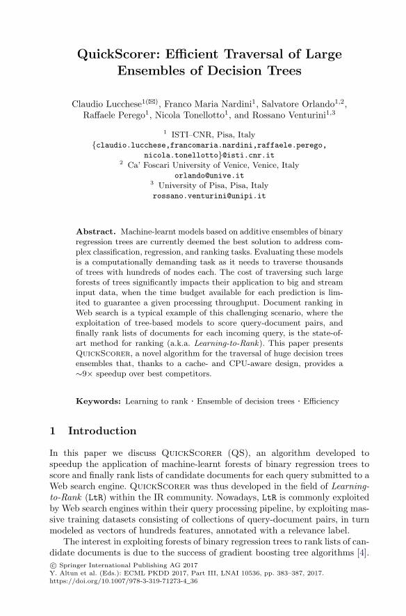
QuickScorer: Efficient Traversal of LargeEnsembles of Decision Trees
Claudio Lucchese1(B), Franco Maria Nardini1, Salvatore Orlando1,2,Raffaele Perego1, Nicola Tonellotto1, and Rossano Venturini1,3
1 ISTI–CNR, Pisa, Italy{claudio.lucchese,francomaria.nardini,raffaele.perego,
nicola.tonellotto}@isti.cnr.it2 Ca’ Foscari University of Venice, Venice, Italy
[email protected] University of Pisa, Pisa, [email protected]
Abstract. Machine-learnt models based on additive ensembles of binaryregression trees are currently deemed the best solution to address com-plex classification, regression, and ranking tasks. Evaluating these modelsis a computationally demanding task as it needs to traverse thousandsof trees with hundreds of nodes each. The cost of traversing such largeforests of trees significantly impacts their application to big and streaminput data, when the time budget available for each prediction is lim-ited to guarantee a given processing throughput. Document ranking inWeb search is a typical example of this challenging scenario, where theexploitation of tree-based models to score query-document pairs, andfinally rank lists of documents for each incoming query, is the state-of-art method for ranking (a.k.a. Learning-to-Rank). This paper presentsQuickScorer, a novel algorithm for the traversal of huge decision treesensembles that, thanks to a cache- and CPU-aware design, provides a∼9× speedup over best competitors.
Keywords: Learning to rank · Ensemble of decision trees · Efficiency
1 Introduction
In this paper we discuss QuickScorer (QS), an algorithm developed tospeedup the application of machine-learnt forests of binary regression trees toscore and finally rank lists of candidate documents for each query submitted to aWeb search engine. QuickScorer was thus developed in the field of Learning-to-Rank (LtR) within the IR community. Nowadays, LtR is commonly exploitedby Web search engines within their query processing pipeline, by exploiting mas-sive training datasets consisting of collections of query-document pairs, in turnmodeled as vectors of hundreds features, annotated with a relevance label.
The interest in exploiting forests of binary regression trees to rank lists of can-didate documents is due to the success of gradient boosting tree algorithms [4].c© Springer International Publishing AG 2017Y. Altun et al. (Eds.): ECML PKDD 2017, Part III, LNAI 10536, pp. 383–387, 2017.https://doi.org/10.1007/978-3-319-71273-4_36

384 C. Lucchese et al.
This kind of algorithms is considered the state-of-the-art LtR solution foraddressing complex ranking problems [5]. In search engines, these forests areexploited within a two-stage architecture. While the first stage retrieves a set ofpossibly relevant documents matching the user query, such expensive LtR-basedscorers, optimized for high precision, are exploited in the second stage to re-rankthe set of candidate documents coming from the first stage. The time budgetavailable to re-rank the candidate documents is limited, due to the incomingrate of queries and the users’ expectations in terms of response time. Therefore,devising techniques and strategies to speed up document ranking without losingin quality is definitely an urgent research topic in Web search [9].
Strongly motivated by these considerations, the IR community has startedto investigate computational optimizations to reduce the scoring time of themost effective LtR rankers based on ensembles of regression trees, by exploitingadvanced features of modern CPUs and carefully exploiting memory hierarchies.Among those, the best competitor of QuickScorer is vPRED [1].
We argue that QuickScorer can also be exploited in different time-sensitivescenarios and each time it is needed to use a large forest of binary decision trees,e.g., random forest, for classification/regression purposes and apply it to big andstream data with strict processing throughput requirements.
2 QuickScorer
Given a query-document pair (q, di), represented by a feature vector x, a LtRmodel based on an additive ensemble of regression trees predicts a relevance scores(x) used for ranking a set of documents. Typically, a tree ensemble encompassesseveral binary decision trees, denoted by T = {T0, T1, . . .}. Each internal (orbranching) node in Th is associated with a Boolean test over a specific featurefφ ∈ F , and a constant threshold γ ∈ R. Tests are of the form x[φ] ≤ γ, and,during the visit, the left branch is taken iff the test succeeds. Each leaf nodestores the tree prediction, representing the potential contribution of the treeto the final document score. The scoring of x requires the traversal of all theensemble’s trees and it is computed as a weighted sum of all the tree predictions.
Algorithm 1 illustrates QS [3,7]. One important result is that QS computess(x) by only identifying the branching nodes whose test evaluates to false, calledfalse nodes. For each false node detected in Th ∈ T , QS updates a bitvector asso-ciated with Th, which stores information that is eventually exploited to identifythe exit leaf of Th that contributes to the final score s(x). To this end, QS main-tains for each tree Th ∈ T a bitvector leafidx[h], made of Λ bits, one per leaf.Initially, every bit in leafidx[h] is set to 1. Moreover, each branching node isassociated with a bitvector mask, still of Λ bits, identifying the set of unreachableleaves of Th in case the corresponding test evaluates to false. Whenever a falsenode is visited, the set of unreachable leaves leafidx[h] is updated througha logical AND (∧) with mask. Eventually, the leftmost bit set in leafidx[h]identifies the leaf corresponding to the score contribution of Th, stored in thelookup table leafvalues.
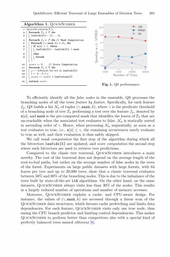
QuickScorer: Efficient Traversal of Large Ensembles of Decision Trees 385
Algorithm 1. QuickScorer1 QuickScorer(x,T):2 foreach Th ∈ T do3 leafidx[h]← 11 . . . 11
4 foreach fφ ∈ F do // Mask Computation5 foreach (γ, mask, h) ∈ Nφ do6 if x[φ] > γ then7 leafidx[h]← leafidx[h] ∧ mask
8 else9 break
10 score ← 0 // Score Computation11 foreach Th ∈ T do12 j ← leftmost bit set in leafidx[h]13 l ← h · Λ + j14 score ← score + leafvalues[l]
15 return score
1000 5000 10000 20000Number of Trees
5
6
7
8
9
10
Speedu
pw.r.t.VPRED
vQS
BWQS
QS
Fig. 1. QS performance.
To efficiently identify all the false nodes in the ensemble, QS processes thebranching nodes of all the trees feature by feature. Specifically, for each featurefφ, QS builds a list Nφ of tuples (γ, mask, h), where γ is the predicate thresholdof a branching node of tree Th performing a test over the feature fφ, denoted byx[φ], and mask is the pre-computed mask that identifies the leaves of Th that areun-reachable when the associated test evaluates to false. Nφ is statically sortedin ascending order of γ. Hence, when processing Nφ sequentially, as soon as atest evaluates to true, i.e., x[φ] ≤ γ, the remaining occurrences surely evaluateto true as well, and their evaluation is thus safely skipped.
We call mask computation the first step of the algorithm during which allthe bitvectors leafidx[h] are updated, and score computation the second stepwhere such bitvectors are used to retrieve tree predictions.
Compared to the classic tree traversal, QuickScorer introduces a mainnovelty. The cost of the traversal does not depend on the average length of theroot-to-leaf paths, but rather on the average number of false nodes in the treesof the forest. Experiments on large public datasets with large forests, with 64leaves per tree and up to 20,000 trees, show that a classic traversal evaluatesbetween 50% and 80% of the branching nodes. This is due to the imbalance of thetrees built by state-of-the-art LtR algorithms. On the other hand, on the samedatasets, QuickScorer always visits less than 30% of the nodes. This resultsin a largely reduced number of operations and number of memory accesses.
Moreover, QuickScorer exploits a cache- and CPU-aware design. Forinstance, the values of (γ, mask, h) are accessed through a linear scan of theQuickScorer data structures, which favours cache prefetching and limits datadependencies. For each feature, QuickScorer visits only one true node, thuseasing the CPU branch predictor and limiting control dependencies. This makesQuickScorer to perform better than competitors also with a special kind ofperfectly balanced trees named oblivious [6].

386 C. Lucchese et al.
The design of QuickScorer makes it possible to introduce two furtherimprovements. Firstly, for large LtR models, the forest can be split into multipleblocks of trees, sufficiently small to allow the data structure of a single block toentirely fit into the third-level CPU cache. We name BlockWise-QS (BWQS)the resulting variant. This cache-aware algorithm reduces the cache miss ratiofrom more than 10% to less than 1%. Secondly, the scoring can be vectorized soas to score multiple documents simultaneously. In V-QuickScorer (vQS) [8]vectorization is achieved through AVX 2.0 instructions and 256-bits wide regis-ters. In such setting, up to 8 documents can be processed simultaneously.
Figure 1 compares QS, BWQS, and vQS against the best competitorvPRED. The test was performed on a large dataset, with a model with 64leaves per tree and varying the number of trees of the forest.
3 Discussion
In this work, we focused on tree ensembles to tackle the LtR problem. Decisiontree ensembles are a popular and effective machine learning tool beyond LtR.Their success is witnessed by the Kaggle 2015 competitions, where most of thewinning solutions exploited MART models, and by the KDD Cup 2015, whereMART-based algorithms were used by all the top 10 teams [2].
In the LtR scenario, the time budget available for applying a model is limitedand must be satisfied. Therefore large models, despite being more accurate,cannot be used because of their high evaluation cost. QS, a novel algorithmfor the traversal of decision trees ensembles, is an answer to this problem asit provides ∼9× speedup over state-of-the-art competitors. Moreover, the needof efficient traversal strategies goes beyond the LtR scenario, for instance whensuch models are used to classify big data collections. For all these reasons, webelieve that QS can help scientists from the data mining community to speed-upthe process of evaluating highly effective tree-based models over big and streamdatasets.
References
1. Asadi, N., Lin, J., de Vries, A.P.: Runtime optimizations for tree-based machinelearning models. IEEE TKDE 26(9), 2281–2292 (2014)
2. Chen, T., Guestrin, C.: XGBoost: A scalable tree boosting system. In: Proceedingsof SIGKDD, pp. 785–794. ACM (2016)
3. Dato, D., Lucchese, C., Nardini, F.M., Orlando, S., Perego, R., Tonellotto, N.,Venturini, R.: Fast ranking with additive ensembles of oblivious and non-obliviousregression trees. ACM TOIS 35(2), 1–31 (2016)
4. Friedman, J.H.: Greedy function approximation: a gradient boosting machine. Ann.Stat. 29, 1189–1232 (2000)
5. Gulin, A., Kuralenok, I., Pavlov, D.: Winning The transfer learning track of yahoo!’slearning to rank challenge with YetiRank. In: Yahoo! Learning to Rank Challenge,pp. 63–76 (2011)

QuickScorer: Efficient Traversal of Large Ensembles of Decision Trees 387
6. Langley, P., Sage, S.: Oblivious decision trees and abstract cases. In: Working Notesof the AAAI-94 Workshop on Case-Based Reasoning, pp. 113–117. AAAI Press(1994)
7. Lucchese, C., Nardini, F.M., Orlando, S., Perego, R., Tonellotto, N., Venturini,R.: QuickScorer: a fast algorithm to rank documents with additive ensembles ofregression trees. In: Proceedings of SIGIR, pp. 73–82. ACM (2015)
8. Lucchese, C., Nardini, F.M., Orlando, S., Perego, R., Tonellotto, N., Venturini, R.:Exploiting CPU SIMD extensions to speed-up document scoring with tree ensem-bles. In: Proceedings of SIGIR, pp. 833–836. ACM (2016)
9. Segalovich, I.: Machine learning in search quality at Yandex. Presentation at theIndustry Track of SIGIR (2010)

Recent Advances in Kernel-BasedGraph Classification
Nils M. Kriege(B) and Christopher Morris
Department of Computer Science, TU Dortmund University, Dortmund, Germany{nils.kriege,christopher.morris}@tu-dortmund.de
Abstract. We review our recent progress in the development of graphkernels. We discuss the hash graph kernel framework, which makes thecomputation of kernels for graphs with vertices and edges annotated withreal-valued information feasible for large data sets. Moreover, we sum-marize our general investigation of the benefits of explicit graph featuremaps in comparison to using the kernel trick. Our experimental studieson real-world data sets suggest that explicit feature maps often providesufficient classification accuracy while being computed more efficiently.Finally, we describe how to construct valid kernels from optimal assign-ments to obtain new expressive graph kernels. These make use of thekernel trick to establish one-to-one correspondences. We conclude by adiscussion of our results and their implication for the future developmentof graph kernels.
1 Introduction
In various domains such as chemo- and bioinformatics, or social network anal-ysis large amounts of graph structured data is becoming increasingly prevalent.Classification of these graphs remains a challenge as most graph kernels eitherdo not scale to large data sets or are not applicable to all types of graphs. In thefollowing we briefly summarize related work before discussing our recent progressin the development of efficient and expressive graphs kernels.
1.1 Related Work
In recent years, various graph kernels have been proposed. Gartner et al. [5]and Kashima et al. [8] simultaneously developed graph kernels based on randomwalks, which count the number of walks two graphs have in common. Since then,random walk kernels have been studied intensively, see, e.g., [7,10,13,19,21].Kernels based on shortest paths were introduced by Borgwardt et al. [1] and arecomputed by performing 1-step walks on the transformed input graphs, whereedges are annotated with shortest-path lengths. A drawback of the approachesmentioned above is their high computational cost. Therefore, a different line ofresearch focuses particularly on scalable graph kernels. These kernels are typi-cally computed by explicit feature maps, see, e.g., [17,18]. This allows to bypassc© Springer International Publishing AG 2017Y. Altun et al. (Eds.): ECML PKDD 2017, Part III, LNAI 10536, pp. 388–392, 2017.https://doi.org/10.1007/978-3-319-71273-4_37

Recent Advances in Kernel-Based Graph Classification 389
the computation of a gram matrix of quadratic size by applying fast linear clas-sifiers [2]. Moreover, graph kernels using assignments have been proposed [4],and were recently applied to geometric embeddings of graphs [6].
2 Recent Progress in the Design of Graph Kernels
We give an overview of our recent progress in the development of scalable andexpressive graph kernels.
2.1 Hash Graph Kernels
In areas such as chemo- or bioinformatics edges and vertices of graphs are oftenannotated with real-valued information, e.g., physical measurements. It has beenshown that these attributes can boost classification accuracies [1,3,9]. Previousgraph kernels that can take these attributes into account are relatively slow andemploy the kernel trick [1,3,9,15]. Therefore, these approaches do not scale tolarge graphs and data sets. In order to overcome this, we introduced the hashgraph kernel framework in [14]. The idea is to iteratively turn the continuousattributes of a graph into discrete labels using randomized hash functions. Thisallows to apply fast explicit graph feature maps, e.g., [17], which are limitedto discrete annotations. In each iteration we sample new hash functions andcompute the feature map. Finally, the feature maps of all iterations are com-bined into one feature map. In order to obtain a meaningful similarity betweenattributes in R
d, we require that the probability of collision Pr[h1(x) = h2(y)]of two independently chosen random hash functions h1, h2 : Rd → N equals anadequate kernel on R
d. Equipped with such a hash function, we derived approx-imation results for several state-of-the-art kernels which can handle continuousinformation. Moreover, we derived a variant of the Weisfeiler-Lehman subtreekernel which can handle continuous attributes.
Our extensive experimental study showed that instances of the hash graphkernel framework achieve state-of-the-art classification accuracies while beingorders of magnitudes faster than kernels that were specifically designed to handlecontinuous information.
2.2 Explicit Graph Feature Maps
Explicit feature maps of kernels for continuous vectorial data are known formany popular kernels like the Gaussian kernel [16] and are heavily applied inpractice. These techniques cannot be used to obtain approximation guaranteesin the hash graph kernel framework. Therefore, in a different line of work, wedeveloped explicit feature maps with the goal to lift the known approximationresults for kernels on continuous data to kernels for graphs annotated with con-tinuous data [11]. More specifically, we investigated how general convolutionkernels are composed from base kernels and how to construct corresponding fea-ture maps. We applied our results to widely used graph kernels and analyzed

390 N. M. Kriege and C. Morris
for which kernels and graph properties computation by explicit feature maps isfeasible and actually more efficient. We derived approximative, explicit featuremaps for state-of-the-art kernels supporting real-valued attributes. Empiricallywe observed that for graph kernels like GraphHopper [3] and Graph Invariant [15]approximative explicit feature maps achieve a classification accuracy close to theexact methods based on the kernel trick, but required only a fraction of theirrunning time. For the shortest-path kernel [1] on the other hand the approachfails in accordance to our theoretical analysis.
Moreover, we investigated the benefits of employing the kernel trick when thenumber of features used by a kernel is very large [10,11]. We derived feature mapsfor random walk and subgraph kernels, and applied them to real-world graphswith discrete labels. Experimentally we observed a phase transition when com-paring running time with respect to label diversity, walk lengths and subgraphsize, respectively, confirming our theoretical analysis.
2.3 Optimal Assignment Kernels
For non-vectorial data, Frohlich et al. [4] proposed kernels for graphs derivedfrom an optimal assignment between their vertices, where vertex attributes arecompared by a base kernel. However, it was shown that the resulting similar-ity measure is not necessarily a valid kernel [20,21]. Hence, in [12], we studiedoptimal assignment kernels in more detail and investigated which base kernelslead to valid kernels. We characterized a specific class of kernels and showedthat it is equivalent to the kernels obtained from a hierarchical partition oftheir domain. When such kernels are used as base kernel the optimal assignment(i) yields a valid kernel; and (ii) can be computed in linear time by histogramintersection given the hierarchy. We demonstrated the versatility of our resultsby deriving novel graph kernels based on optimal assignments, which are shownto improve over their convolution-based counterparts. In particular, we proposedthe Weisfeiler-Lehman optimal assignment kernel, which performs favorable com-pared to state-of-the-art graph kernels on a wide range of data sets.
3 Conclusion
We gave an overview about our recent progress in kernel-based graph classifica-tion. Our results show that explicit graph feature maps can provide an efficientcomputational alternative for many known graph kernels and practical applica-tions. This is the case for kernels supporting graphs with continuous attributesand for those limited to discrete labels, even when the number of features is verylarge. Assignment kernels, on the other hand, are computed by histogram inter-section and thereby again employ the kernel trick. This suggests to study theapplication of non-linear kernels to explicit graph feature maps in more detailas future work.

Recent Advances in Kernel-Based Graph Classification 391
Acknowledgement. We would like to thank the co-authors of our publications [10–12,14]. This research was supported by the German Science Foundation (DFG) withinthe Collaborative Research Center SFB 876 “Providing Information by Resource-Constrained Data Analysis”, project A6.
References
1. Borgwardt, K.M., Kriegel, H.P.: Shortest-path kernels on graphs. In: IEEE Inter-national Conference on Data Mining, pp. 74–81 (2005)
2. Fan, R.E., Chang, K.W., Hsieh, C.J., Wang, X.R., Lin, C.J.: LIBLINEAR: a libraryfor large linear classification. J. Mach. Learn. Res. 9, 1871–1874 (2008)
3. Feragen, A., Kasenburg, N., Petersen, J., Bruijne, M.D., Borgwardt, K.: Scalablekernels for graphs with continuous attributes. In: Advances in Neural InformationProcessing Systems, pp. 216–224 (2013)
4. Frohlich, H., Wegner, J.K., Sieker, F., Zell, A.: Optimal assignment kernels forattributed molecular graphs. In: 22nd International Conference on Machine Learn-ing, pp. 225–232 (2005)
5. Gartner, T., Flach, P., Wrobel, S.: On graph kernels: hardness results and efficientalternatives. In: Scholkopf, B., Warmuth, M.K. (eds.) COLT-Kernel 2003. LNCS(LNAI), vol. 2777, pp. 129–143. Springer, Heidelberg (2003). https://doi.org/10.1007/978-3-540-45167-9 11
6. Johansson, F.D., Dubhashi, D.: Learning with similarity functions on graphs usingmatchings of geometric embeddings. In: 21st ACM SIGKDD International Confer-ence on Knowledge Discovery and Data Mining, pp. 467–476 (2015)
7. Kang, U., Tong, H., Sun, J.: Fast random walk graph kernel. In: SIAM InternationalConference on Data Mining, pp. 828–838 (2012)
8. Kashima, H., Tsuda, K., Inokuchi, A.: Marginalized kernels between labeledgraphs. In: 20th International Conference on Machine Learning, pp. 321–328 (2003)
9. Kriege, N., Mutzel, P.: Subgraph matching kernels for attributed graphs. In: 29thInternational Conference on Machine Learning (2012)
10. Kriege, N., Neumann, M., Kersting, K., Mutzel, M.: Explicit versus implicit graphfeature maps: a computational phase transition for walk kernels. In: IEEE Inter-national Conference on Data Mining, pp. 881–886 (2014)
11. Kriege, N.M., Neumann, M., Morris, C., Kersting, K., Mutzel, P.: A unifying viewof explicit and implicit feature maps for structured data: Systematic studies ofgraph kernels. CoRR abs/1703.00676 (2017). http://arxiv.org/abs/1703.00676
12. Kriege, N.M., Giscard, P.-L., Wilson, R.C.: On valid optimal assignment kernelsand applications to graph classification. In: Advances in Neural Information Pro-cessing Systems, pp. 1615–1623 (2016)
13. Mahe, P., Ueda, N., Akutsu, T., Perret, J.L., Vert, J.P.: Extensions of marginalizedgraph kernels. In: Twenty-First International Conference on Machine Learning, pp.552–559 (2004)
14. Morris, C., Kriege, N.M., Kersting, K., Mutzel, P.: Faster kernel for graphs withcontinuous attributes via hashing. In: IEEE International Conference on Data Min-ing, pp. 1095–1100 (2016)
15. Orsini, F., Frasconi, P., De Raedt, L.: Graph invariant kernels. In: Twenty-FourthInternational Joint Conference on Artificial Intelligence, pp. 3756–3762 (2015)
16. Rahimi, A., Recht, B.: Random features for large-scale kernel machines. In:Advances in Neural Information Processing Systems, pp. 1177–1184 (2008)

392 N. M. Kriege and C. Morris
17. Shervashidze, N., Schweitzer, P., van Leeuwen, E.J., Mehlhorn, K., Borgwardt,K.M.: Weisfeiler-Lehman graph kernels. J. Mach. Learn. Res. 12, 2539–2561 (2011)
18. Shervashidze, N., Vishwanathan, S.V.N., Petri, T.H., Mehlhorn, K., Borgwardt,K.M.: Efficient graphlet kernels for large graph comparison. In: Twelfth Interna-tional Conference on Artificial Intelligence and Statistics, pp. 488–495 (2009)
19. Sugiyama, M., Borgwardt, K.M.: Halting in random walk kernels. In: Advances inNeural Information Processing Systems, pp. 1639–1647 (2015)
20. Vert, J.P.: The optimal assignment kernel is not positive definite. CoRRabs/0801.4061 (2008). http://arxiv.org/abs/0801.4061
21. Vishwanathan, S.V.N., Schraudolph, N.N., Kondor, R., Borgwardt, K.M.: Graphkernels. J. Mach. Learn. Res. 11, 1201–1242 (2010)

Demo Track

ASK-the-Expert: Active Learning BasedKnowledge Discovery Using the Expert
Kamalika Das1(B), Ilya Avrekh2, Bryan Matthews2, Manali Sharma3,and Nikunj Oza4
1 USRA, NASA Ames Research Center, Moffett Field, Moffett Field, CA, [email protected]
2 SGT Inc., NASA Ames Research Center, Moffett Field, Moffett Field, CA, USA{ilya.avrekh-1,bryan.l.matthews}@nasa.gov
3 Samsung Semiconductor Inc., San Jose, CA, [email protected]
4 NASA Ames Research Center, Moffett Field, Moffett Field, CA, [email protected]
Abstract. Often the manual review of large data sets, either forpurposes of labeling unlabeled instances or for classifying meaningfulresults from uninteresting (but statistically significant) ones is extremelyresource intensive, especially in terms of subject matter expert (SME)time. Use of active learning has been shown to diminish this reviewtime significantly. However, since active learning is an iterative processof learning a classifier based on a small number of SME-provided labelsat each iteration, the lack of an enabling tool can hinder the process ofadoption of these technologies in real-life, in spite of their labor-savingpotential. In this demo we present ASK-the-Expert, an interactive toolthat allows SMEs to review instances from a data set and provide labelswithin a single framework. ASK-the-Expert is powered by an activelearning algorithm for training a classifier in the backend. We demon-strate this system in the context of an aviation safety application, butthe tool can be adopted to work as a simple review and labeling tool aswell, without the use of active learning.
Keywords: Active learning · Graphical user interface · ReviewLabeling
1 Introduction
Active learning is an iterative process that requires feedback on instances froma subject matter expert (SME) in an interactive fashion. The idea in active
M. Sharma—This work was done when the author was a student at Illinois Instituteof Technology.The rights of this work are transferred to the extent transferable according to title17 U.S.C. 105.
c© Springer International Publishing AG 2017Y. Altun et al. (Eds.): ECML PKDD 2017, Part III, LNAI 10536, pp. 395–399, 2017.https://doi.org/10.1007/978-3-319-71273-4_38
396 K. Das et al.
learning is to bootstrap an initial classifier with a few examples from each classthat have been labeled by the SME. Traditional active learning approaches selectan informative instance from the unlabeled data set and ask SMEs to review theinstance and provide a label. This process continues iteratively until a desiredlevel of performance is achieved by the classifier or when the budget (allottedresources) for the SME is exhausted. Much of the research in active learningsimulates this interaction between the learner and the SME. In particular, alllabels are collected from the SME a priori and during the active learning process,the relevant labeled instances are revealed to the learner, based on its requests ateach iteration. The problem of using such retrospective evaluation of an activelearning algorithm is twofold. Firstly, the lack of availability of an interactiveinterface is largely responsible for the generally low adoption of active learningalgorithms in practical scenarios. Secondly, the simulated environment fails toachieve the biggest benefit associated with the use of active learning: reduction ofSME review time. This is because the SME has to review and label all examplesa priori. Therefore, for utilizing active learning frameworks in situations of lowavailability of labeled data, it is important to have an interactive tool that allowsSMEs to review and label instances only when asked by the learner.
2 Application and Demo Scenario
A major focus of the commercial aviation community is discovery of unknownsafety events in flight operational data through the use of unsupervised anomalydetection algorithms. However, anomalies found using such approaches areabnormal only in the statistical sense, i.e., they may or may not represent anoperationally significant event (e.g. represent a real safety concern). After analgorithm produces a list of statistical anomalies, an SME must review the listto identify those that are operationally relevant for further investigation. Usually,less than 1% of the hundreds or thousands of statistical anomalies turn out to beoperationally relevant. Therefore, substantial time and effort is spent examininganomalies that are not of interest and it is essential to optimize this review pro-cess in order to reduce SME labeling efforts (man hours spent in investigatingresults). A recently developed active learning method [2] incorporates SME feed-back in the form of rationales for classification of flights to build a classifier thatcan distinguish between uninteresting and operationally significant anomalieswith 70% fewer labels compared to manual review and comparable accuracy.
To the best of our knowledge, there exists no published work that describessuch software tools for review and annotation of numerical data using activelearning. There are some image and video annotation tools that collect labels,such as LabelMe from MIT CSAIL [1]. Additionally there are active learningpowered text labeling tools, such as Abstrackr [3] designed specifically for medi-cal experts for citation review and labeling. The major difference between theseannotator tools and our tool is the absence of context in our case. Unlike in thecase of image or text data where the information is self-contained in the instancebeing reviewed, in our case, we have to enable the tool to obtain additional con-textual information and visualize the feature space on demand. Other domains
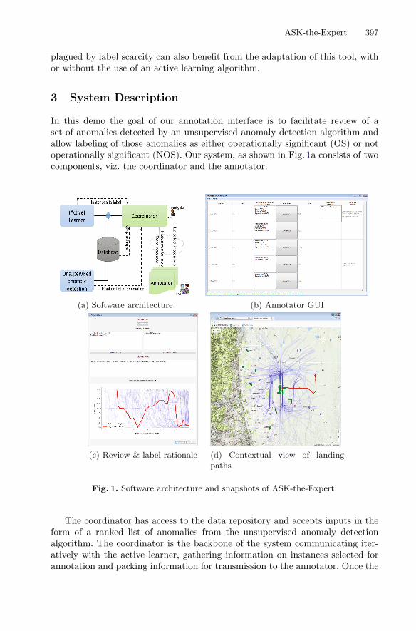
ASK-the-Expert 397
plagued by label scarcity can also benefit from the adaptation of this tool, withor without the use of an active learning algorithm.
3 System Description
In this demo the goal of our annotation interface is to facilitate review of aset of anomalies detected by an unsupervised anomaly detection algorithm andallow labeling of those anomalies as either operationally significant (OS) or notoperationally significant (NOS). Our system, as shown in Fig. 1a consists of twocomponents, viz. the coordinator and the annotator.
(a) Software architecture (b) Annotator GUI
(c) Review & label rationale (d) Contextual view of landingpaths
Fig. 1. Software architecture and snapshots of ASK-the-Expert
The coordinator has access to the data repository and accepts inputs in theform of a ranked list of anomalies from the unsupervised anomaly detectionalgorithm. The coordinator is the backbone of the system communicating iter-atively with the active learner, gathering information on instances selected forannotation and packing information for transmission to the annotator. Once the

398 K. Das et al.
annotator collects and sends the labeled instances, the coordinator performs twotasks: (i) resolve labeling conflicts across multiple SMEs through the use of amajority voting scheme or by invoking an investigator review, and (ii) automatethe construction of new rationale features as conjunctions and/or disjunctionsof raw data features based on the rationale notes entered by the SME in theannotation window. All data exchange between the coordinator and the anno-tator happens through cloud based storage. The annotator, shown in Fig. 1b isthe graphical user interface that the SMEs work with and needs to be installedat the SME end. When the annotator is opened, it checks for new data packets(to be labeled) on the cloud. If new examples need annotation, the annotatorwindow displays the list of examples ranked in the order of importance alongwith the features identified to be the most anomalous. Clicking on the annotatebutton next to each example, the SME can delve deeper into that example inorder to provide a label for that instance. The functions of the annotator include(i) obtaining examples to be labeled from the cloud and displaying them to theSME, (ii) allowing review of individual features as well as feature interactions(shown in Fig. 1c), and (iii) occasionally providing additional context informa-tion by looking at additional data sources (for example, plotting flight pathsin the context of other flights landing on the same runway at a certain airportusing geographical data from maps, as shown in Fig. 1d). Multiple annotatorscan be used simultaneously by different SMEs to label the same or different setsof examples. Once the labeled examples are submitted by the annotator, thecoordinator collects and consolidates them and sends them back to the learner.
Demo Plan: We will demonstrate the ASK-the-Expert tool for an aviationsafety case study. Since the data cubes for normal and anomalous flights are pro-prietary information, the database will be hosted in our laptop. The coordinatortool will be live and running at NASA, gathering the latest set of flights thatneed to be labeled and uploading them on the cloud. We will demonstrate howthe SMEs can review new examples in the context of other flights and providelabels. Their feedback will be sent back to the learner through the coordina-tor for the next iteration of classifier learning after incorporating new rationalefeatures.
Acknowledgments. This work is supported in part by a Center Innovation Fund(CIF) 2017 grant at NASA Ames Research Center and in part by the NASA Aero-nautics Mission Directorate. Manali Sharma was supported by the National ScienceFoundation CAREER award no. IIS-1350337.

ASK-the-Expert 399
References
1. Russell, B., Torralba, A., Murphy, K., Freeman, W.: LabelMe: a database and web-based tool for image annotation. Int. J. Comput. Vis. 77(1), 157–173 (2007)
2. Sharma, M., Das, K., Bilgic, M., Matthews, B., Nielsen, D., Oza, N.: Active learningwith rationales for identifying operationally significant anomalies in aviation. In:Proceedings of European Conference on Machine Learning and Knowledge Discoveryin Databases, ECML-PKDD 2016, pp. 209–225 (2016)
3. Wallace, B., Small, K., Brodley, C., Lau, J., Trikalinos, T.: Deploying an interac-tive machine learning system in an evidence-based practice center: Abstrackr. In:Proceedings of the 2nd ACM SIGHIT International Health Informatics Symposium,pp. 819–824 (2012)
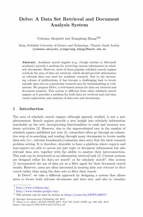
Delve: A Data Set Retrieval and DocumentAnalysis System
Uchenna Akujuobi and Xiangliang Zhang(B)
King Abdullah University of Science and Technology, Thuwal, Saudi Arabia{uchenna.akujuobi,xiangliang.zhang}@kaust.edu.sa
Abstract. Academic search engines (e.g., Google scholar or Microsoftacademic) provide a medium for retrieving various information on schol-arly documents. However, most of these popular scholarly search enginesoverlook the area of data set retrieval, which should provide informationon relevant data sets used for academic research. Due to the increas-ing volume of publications, it has become a challenging task to locatesuitable data sets on a particular research area for benchmarking or eval-uations. We propose Delve, a web-based system for data set retrieval anddocument analysis. This system is different from other scholarly searchengines as it provides a medium for both data set retrieval and real timevisual exploration and analysis of data sets and documents.
1 Introduction
The area of scholarly search engines although sparsely studied, is not a newphenomenon. Search engines provide a new insight into scholarly informationsearchable on the web, incorporating functionalities to rank and measure aca-demic activities [3]. However, due to the unprecedented rate in the number ofscholarly papers published per year [4], researchers often go through an exhaus-tive step of re-searching and reading through many documents to locate usabledata sets (i.e., relevant benchmark/evaluation data sets) that fits their researchproblem setting. It is therefore, desirable to have a platform where experts andnon-experts are able to access not just topic or document information but alsorelevant data sets, together with the ability to analyze their interconnection.This task can be structured as an information retrieval task [5]. Current systemsare designed either for data set search1 or for scholarly search2. One system[1] incorporated the use of data set as a filter agent for their document searchresults. However, users are often interested in locating data sets relevant to theirsearch rather than using the data sets to filter their search.
In Delve3, we take a different approach by designing a system that allowsusers to locate both relevant documents and data sets, and also to visualize
1 http://www.re3data.org/.2 http://www.scholar.google.com/.3 The system can be seen in action at https://youtu.be/bF6PUj8801U.
c© Springer International Publishing AG 2017Y. Altun et al. (Eds.): ECML PKDD 2017, Part III, LNAI 10536, pp. 400–403, 2017.https://doi.org/10.1007/978-3-319-71273-4_39

Delve: A Data Set Retrieval and Document Analysis System 401
and analyze their relationship network. Delve borrows ideas from label propaga-tion [2] algorithm and adopts methods proposed in ParsCit [6] for text mining.Our system also provides a simple and easy-to-use interface built on the d3.js4
framework which facilitates visualization and analysis of papers and data sets.
2 System Design
Our data set was constructed with an initial focus on academic documents pub-lished in 17 different conferences and journals between 2001 to 2015, includ-ing ICDE, KDD, TKDE, VLDB, CIKM, NIPS, ICML, ICDM, PKDD, SDM,WSDM, AAAI, IJCAI, DMKD, WWW, KAIS and TKDD. Using the Microsoftgraph data set5, we then extended these documents, adding their references andthe references of their references (up to 2 hops away). In total, we currently have2,116,429 academic publications from more than 1000 different conferences andjournals.
Data Set and Document Analysis. Our system is built on the citation graphof these more than 2 million papers. Formally, in a directed citation graph G ={V,E}, two nodes vi and vj are linked by edge E(vi; vj) if vi cites vj . Since thesystem is designed for data set relevant retrieval, an edge E(vi; vj) between vi andvj can be labeled as: 1 - if vi cites vj because vi uses the data set available/usedin vj ; and 0 - otherwise. Then based on the labels, we can extract the data setlabeled citations. The initial labeling work was conducted by crowd-sourcing onpapers and data sets cited by papers published in ICDE, KDD, ICDM, SDM andTKDE from 2001 to 2014. These labels (accounting for 5% of the whole graphedges) have been manually verified to be correct by three qualified participants.Due to the high cost, it is infeasible to label the remaining 95% of edges manually.Therefore, the main challenging task is to develop a correct and yet efficientalgorithm to efficiently assign labels to the large amount of unlabeled edgesusing the limited amount of verified labels. To solve this problem, we developeda semi-supervised learning method “link label propagation algorithm” usingideas borrowed from label propagation algorithm [2].
Label Assignment. The original label propagation (LP) algorithm predictslabels for nodes, our task is to predict labels for edges. Therefore we restructurethe original graph to G′ = {V ′, E′} where V ′ is the set of edges E in graph G,and E′ is the set of generated edges. The edges E′ are generated by linking eachedge Ei in G (V ′
i in G′) to the top 10 similar edges Ej (V ′j in G′) that have the
same target node as Ei or where the target node of Ei is the source node of Ej .To define the similarity between citations, we extract the number of data setkeywords6 from each citation context (i.e. the sentences which encompass thecitations). We then defined a Gaussian similarity score between pairs of edges(Ei, Ej) Simij = exp(−‖di−dj‖2
2σ2 ), where di = nd
nc. nd is the number of data set
4 https://d3js.org/.5 https://academicgraph.blob.core.windows.net/graph-2015-11-06/index.html.6 Manually compiled list of data set related words.
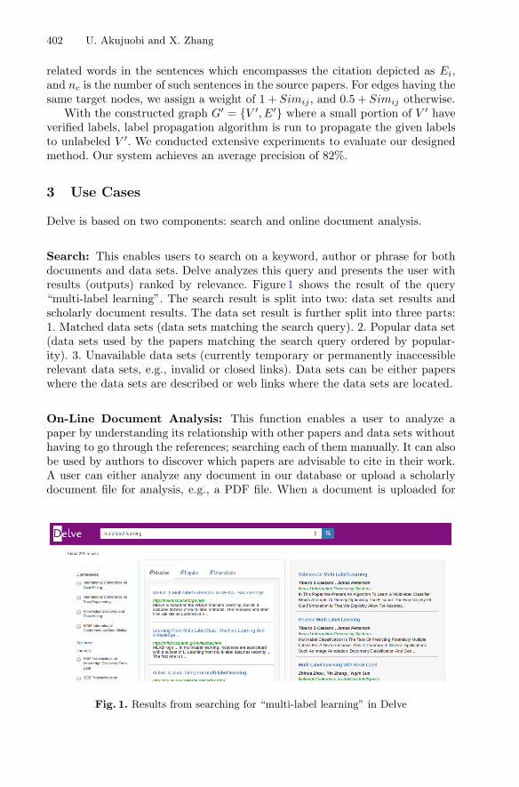
402 U. Akujuobi and X. Zhang
related words in the sentences which encompasses the citation depicted as Ei,and nc is the number of such sentences in the source papers. For edges having thesame target nodes, we assign a weight of 1 + Simij , and 0.5 + Simij otherwise.
With the constructed graph G′ = {V ′, E′} where a small portion of V ′ haveverified labels, label propagation algorithm is run to propagate the given labelsto unlabeled V ′. We conducted extensive experiments to evaluate our designedmethod. Our system achieves an average precision of 82%.
3 Use Cases
Delve is based on two components: search and online document analysis.
Search: This enables users to search on a keyword, author or phrase for bothdocuments and data sets. Delve analyzes this query and presents the user withresults (outputs) ranked by relevance. Figure 1 shows the result of the query“multi-label learning”. The search result is split into two: data set results andscholarly document results. The data set result is further split into three parts:1. Matched data sets (data sets matching the search query). 2. Popular data set(data sets used by the papers matching the search query ordered by popular-ity). 3. Unavailable data sets (currently temporary or permanently inaccessiblerelevant data sets, e.g., invalid or closed links). Data sets can be either paperswhere the data sets are described or web links where the data sets are located.
On-Line Document Analysis: This function enables a user to analyze apaper by understanding its relationship with other papers and data sets withouthaving to go through the references; searching each of them manually. It can alsobe used by authors to discover which papers are advisable to cite in their work.A user can either analyze any document in our database or upload a scholarlydocument file for analysis, e.g., a PDF file. When a document is uploaded for
Fig. 1. Results from searching for “multi-label learning” in Delve

Delve: A Data Set Retrieval and Document Analysis System 403
Fig. 2. Final output of uploaded file analysis in Delve (Color figure online)
analysis, Delve mines and analyzes the document text, translates the results as aquery and displays the result as a visual citation graph, as shown in Fig. 2, whichgives the result of analyzing Multi-label methods for prediction with sequentialdata [7]. We would like to point out that this paper is not in our system at themoment of writing this paper. However, based on its references and citations,our system can analyze its relevant papers and visualize the citation relations.
Note that in Fig. 2, the blue edges indicate data set relevant relationships,and the size of the nodes show its importance in the network measured basedits citations in the subgraph. Mouse hovering over a node displays the item titleand clicking on a node displays more information about the item. In addition,the red edges show a non data set relevant relationship, and broken edges haveunknown labels. The unknown labels can be inferred using label propagation.
References
1. Semantic Scholar: Web. https://www.semanticscholar.org. Accessed 21 Feb 20172. Fujiwara, Y., Irie, G.: Efficient label propagation. In: ICML-2014 (2014)3. Ortega, J.L.: Academic Search Engines: A Quantitative Outlook. Elsevier (2014)4. National Science Board: Science and engineering indicators. National Science Foun-
dation, Arlington (2012)5. Sathiaseelan, J.G.R.: A technical study on Information Retrieval using web mining
techniques. In: ICIIECS (2015)6. Councill, I.G., et al.: ParsCit: an open-source CRF reference string parsing package.
In: LREC (2008)7. Read, J., et al.: Multi-label methods for prediction with sequential data. Pattern
Recognit. 63, 45–55 (2017)
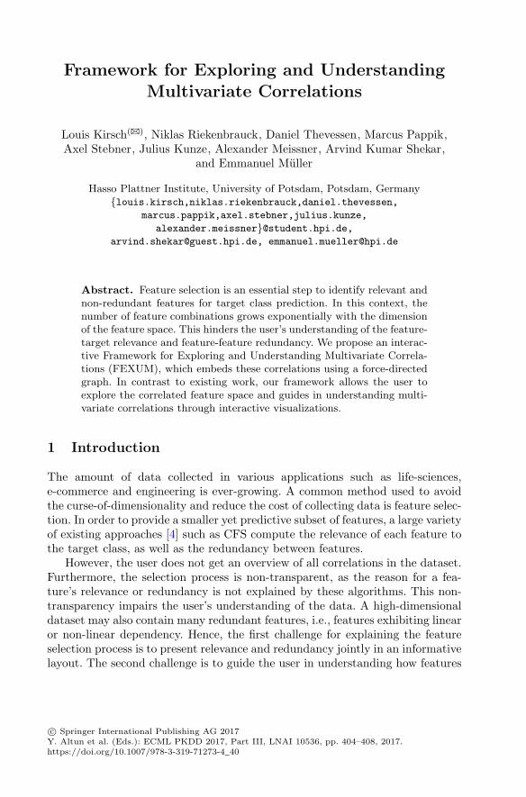
Framework for Exploring and UnderstandingMultivariate Correlations
Louis Kirsch(B), Niklas Riekenbrauck, Daniel Thevessen, Marcus Pappik,Axel Stebner, Julius Kunze, Alexander Meissner, Arvind Kumar Shekar,
and Emmanuel Muller
Hasso Plattner Institute, University of Potsdam, Potsdam, Germany{louis.kirsch,niklas.riekenbrauck,daniel.thevessen,
marcus.pappik,axel.stebner,julius.kunze,
alexander.meissner}@student.hpi.de,[email protected], [email protected]
Abstract. Feature selection is an essential step to identify relevant andnon-redundant features for target class prediction. In this context, thenumber of feature combinations grows exponentially with the dimensionof the feature space. This hinders the user’s understanding of the feature-target relevance and feature-feature redundancy. We propose an interac-tive Framework for Exploring and Understanding Multivariate Correla-tions (FEXUM), which embeds these correlations using a force-directedgraph. In contrast to existing work, our framework allows the user toexplore the correlated feature space and guides in understanding multi-variate correlations through interactive visualizations.
1 Introduction
The amount of data collected in various applications such as life-sciences,e-commerce and engineering is ever-growing. A common method used to avoidthe curse-of-dimensionality and reduce the cost of collecting data is feature selec-tion. In order to provide a smaller yet predictive subset of features, a large varietyof existing approaches [4] such as CFS compute the relevance of each feature tothe target class, as well as the redundancy between features.
However, the user does not get an overview of all correlations in the dataset.Furthermore, the selection process is non-transparent, as the reason for a fea-ture’s relevance or redundancy is not explained by these algorithms. This non-transparency impairs the user’s understanding of the data. A high-dimensionaldataset may also contain many redundant features, i.e., features exhibiting linearor non-linear dependency. Hence, the first challenge for explaining the featureselection process is to present relevance and redundancy jointly in an informativelayout. The second challenge is to guide the user in understanding how features
c© Springer International Publishing AG 2017Y. Altun et al. (Eds.): ECML PKDD 2017, Part III, LNAI 10536, pp. 404–408, 2017.https://doi.org/10.1007/978-3-319-71273-4_40

Framework for Exploring and Understanding Multivariate Correlations 405
are correlated as opposed to merely returning a correlation score. We addressthese two challenges by contributing FEXUM, a framework that provides:
(1) A visual embedding of feature correlations (relevances and redundancies).(2) User-reviewable multivariate correlations.
This leads to a more comprehensible selection process in comparison to state-of-the-art tools, reflected in Table 1. While most tools focus on fully-automatedstatistical selection of features, with FEXUM we aim at explaining traditionalblack-box algorithms. KNIME is a renowned tool that offers filter-based fea-ture selection using linear correlation and variance measures. However, withoutcustomized extensions, it does not address feature redundancy during selection.RapidMiner and Weka take redundancy into account, but do not provide anoverview of all feature correlations. Additionally, they do not explain the reasonfor the relevance of a feature.
Table 1. Comparison of feature selection tools
Tools Relevance Redundancy Correlation overview Correlation explanation
KNIME ✓ ✗ ✗ ✗RapidMiner ✓ ✓ ✗ ✗Weka ✓ ✓ ✗ ✗FEXUM ✓ ✓ ✓ ✓
2 FEXUM
FEXUM is an application that allows instant access with a web browser. Weachieve this by basing our infrastructure on AngularJS and the Django webframework. To ensure scalability for large datasets, we distribute computationsto multiple machines with Celery. The entire framework is open source andavailable online1.
2.1 Relevance-Redundancy Embedding
As explained in Sect. 1, existing feature ranking methods do not provide a com-prehensive overview of correlations that facilitate exploring the dataset. There-fore, our goal is to simultaneously visualize all feature correlations to the target(relevance) and pairwise correlations (redundancy). We allow for arbitrary rele-vance and redundancy measures. For now, we employ the concept of conditionaldependence from [2] to quantify the correlations.
However, it is computationally expensive to calculate the redundancy scorefor all feature pairs. We propose, hence, to infer the redundancy scores heuristi-cally from random subsets. The pseudo-code for this computation is made avail-able online2. Our visualization provides a layout in which a smaller distance of a1 https://github.com/KDD-OpenSource/fexum.2 https://github.com/KDD-OpenSource/fexum-hics/blob/master/FPR.pdf.
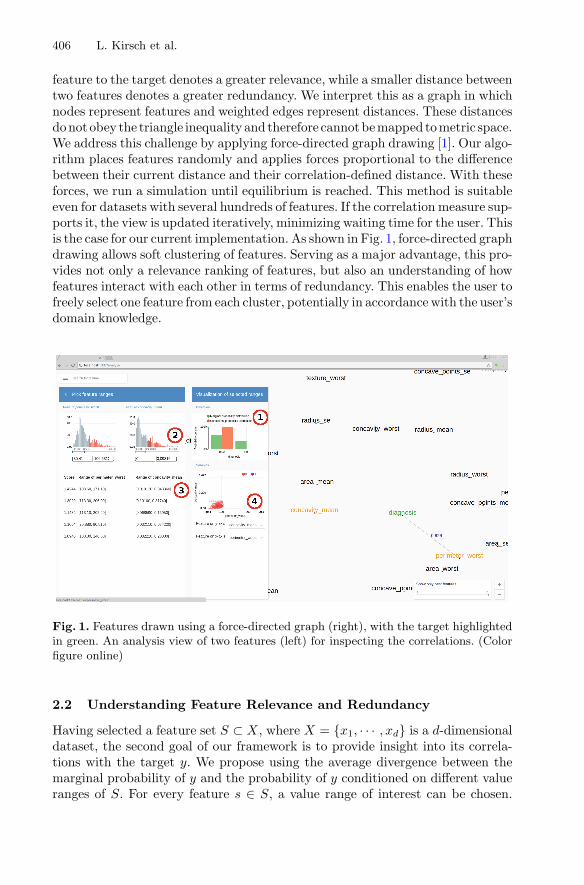
406 L. Kirsch et al.
feature to the target denotes a greater relevance, while a smaller distance betweentwo features denotes a greater redundancy. We interpret this as a graph in whichnodes represent features and weighted edges represent distances. These distancesdonot obey the triangle inequality and therefore cannotbemapped tometric space.We address this challenge by applying force-directed graph drawing [1]. Our algo-rithm places features randomly and applies forces proportional to the differencebetween their current distance and their correlation-defined distance. With theseforces, we run a simulation until equilibrium is reached. This method is suitableeven for datasets with several hundreds of features. If the correlation measure sup-ports it, the view is updated iteratively, minimizing waiting time for the user. Thisis the case for our current implementation. As shown in Fig. 1, force-directed graphdrawing allows soft clustering of features. Serving as a major advantage, this pro-vides not only a relevance ranking of features, but also an understanding of howfeatures interact with each other in terms of redundancy. This enables the user tofreely select one feature from each cluster, potentially in accordance with the user’sdomain knowledge.
Fig. 1. Features drawn using a force-directed graph (right), with the target highlightedin green. An analysis view of two features (left) for inspecting the correlations. (Colorfigure online)
2.2 Understanding Feature Relevance and Redundancy
Having selected a feature set S ⊂ X, where X = {x1, · · · , xd} is a d-dimensionaldataset, the second goal of our framework is to provide insight into its correla-tions with the target y. We propose using the average divergence between themarginal probability of y and the probability of y conditioned on different valueranges of S. For every feature s ∈ S, a value range of interest can be chosen.

Framework for Exploring and Understanding Multivariate Correlations 407
If a feature s correlates with the target feature y, there exists a value range of swhich changes the distribution of y in contrast to y’s marginal distribution [2].
As shown in Fig. 1, our framework allows specifying the respective valuerange per feature using value sliders. Therefore, both bivariate and multivariatecorrelations can be detected. Our framework guides the user with four essentialcomponents for understanding correlations with the target.
Both the target’s marginal probability distribution and the distribution con-ditioned on the selected value ranges are rendered in Fig. 1: (1). Changing valueranges updates this plot in real-time, allowing the user to test hypotheses evalu-ated according to the resulting divergence from the marginal distribution. Iden-tifying the right hypotheses becomes challenging with more features to consider.To address this, value ranges that maximally violate the assumption of sta-tistical independence w.r.t. the target feature are highlighted in a histogramabove the sliders in (2). This tells the user which ranges strongly contribute tobivariate correlations. Nevertheless, it is still difficult to find multivariate cor-relations. Therefore, a table in (3) suggests multiple configurations, where eachconfiguration specifies a value range for each s ∈ S. Each configuration is scoredbased on the divergence of its probability distribution and only the highest scor-ing configurations are displayed. Selecting one of these suggestions updates therespective value range sliders and the probability distribution plot. Finally, incase y is categorical, we visualize the data points within the value ranges in ourtwo dimensional scatter plot in (4), each data point colorized according to itsrespective class.
2.3 Demonstration
FEXUM can be used with a wide range of datasets, supplied through upload bythe user. While it is currently in use in industry, we will demonstrate our frame-work on publicly available datasets from medical, social and physical applica-tions. As an example, we now show how our framework enhances feature selectionfor the Wisconsin Breast Cancer (Diagnostic) dataset [3] in Fig. 1.
In the rendering of our force-directed graph, we observe varied feature rele-vance scores and clusters of redundant features. In particular, features derivedfrom similar properties such as radius mean and radius worst achieve compa-rable relevances and are highly redundant to each other. Based on this firstimpression, we decide to have a closer look at the most relevant feature perime-ter worst . We can easily find influential value ranges in the analysis view, becausethey are highlighted in red in the histogram. The overall relevance score can becorroborated by analyzing several individual value ranges, which can be chosenbased on the framework’s recommendations or expert knowledge.
Since we support multivariate correlations, the current subset can be itera-tively expanded in a similar fashion. As demonstrated, the framework guides inexploration and review of correlations.

408 L. Kirsch et al.
References
1. Fruchterman, T.M., Reingold, E.M.: Graph drawing by force-directed placement.Softw. Pract. Exp. 21(11), 1129–1164 (1991)
2. Keller, F., Muller, E., Bohm, K.: HiCS: high contrast subspaces for density-basedoutlier ranking. In: ICDE (2012)
3. Lichman, M.: UCI machine learning repository (2013). http://archive.ics.uci.edu/ml.Accessed 17 Apr 2017
4. Molina, L.C., Belanche, L., Nebot, A.: Feature selection algorithms: a survey andexperimental evaluation. In: ICDM (2003)
Lit@EVE : Explainable Recommendation Basedon Wikipedia Concept Vectors
M. Atif Qureshi(B) and Derek Greene
Insight Center for Data Analytics, University College Dublin,Dublin, Republic of Ireland
{muhammad.qureshi,derek.greene}@ucd.ie
Abstract. We present an explainable recommendation system fornovels and authors, called Lit@EVE, which is based on Wikipedia con-cept vectors. In this system, each novel or author is treated as a conceptwhose definition is extracted as a concept vector through the applicationof an explainable word embedding technique called EVE. Each dimen-sion of the concept vector is labelled as either a Wikipedia article or aWikipedia category name, making the vector representation readily inter-pretable. In order to recommend items, the Lit@EVE system uses thesevectors to compute similarity scores between a target novel or author andall other candidate items. Finally, the system generates an ordered listof suggested items by showing the most informative features as human-readable labels, thereby making the recommendation explainable.
1 Introduction
Recently, considerable attention has been paid to providing meaningful explana-tions for decisions made by algorithms [5]. On the legislative side, the EuropeanUnion has approved regulations that requires a “right to explanation” in relationto any user-facing algorithm [2]. This increased emphasis on the need for explain-able decision-making algorithms is the first motivation for our work. As furthermotivation, increasingly recommender systems attempt to offer serendipitoussuggestions, where the items being recommended are relevant but also poten-tially different from those items which they users seen previously [3]. To addressboth of these motivations, we propose the Lit@EVE system, which makes useof Wikipedia articles and categories as a rich source of structured features.Furthermore, to explain the similarity between items, the system makes useof our previously-proposed word embedding algorithm called EVE [6]. Wordembedding algorithms generate real-valued representation for words or conceptsin a vector space, allowing simple comparisons to be made between them by oper-ating over their corresponding vectors. In the case of EVE, the dimensions ofthis space are human-readable, as each dimension represents a single Wikipediaarticle or category. We demonstrate this approach in the context of recommend-ing books and authors, where EVE concept vectors are used to represent bothauthors and their literary works.c© Springer International Publishing AG 2017Y. Altun et al. (Eds.): ECML PKDD 2017, Part III, LNAI 10536, pp. 409–413, 2017.https://doi.org/10.1007/978-3-319-71273-4_41

410 M. A. Qureshi and D. Greene
Recently, Chang et al. [1] described a crowdsourcing-based framework forgenerating natural language explanations which relies on specific human-generated annotations, whereas our system harnesses the ongoing work ofWikipedia editors, and automatically assigns labels to explain a given recom-mendation. Moreover, the use of a rich set of Wikipedia articles and categoriesas features helps to highlight serendipitous aspects of recommended items whichare otherwise difficult to discover.
2 System Overview
We now present an overview of the Lit@EVE system. First, we discuss thedataset used to build our recommender, then we discuss the corresponding EVEword embeddings, and finally we show how recommendations are generated usingthe system.
2.1 Dataset
Our dataset is based on the curated “Wikiproject novels”1 list which contains49,999 Wikipedia entries (as of 20 April 2017) relating to literature. Many ofthese entries correspond to novels, although some denote other literary concepts,such as genres, publishers, and tropes. In order to exclusively extract novels,we include only those with a Wikipedia info box that contains an “author”attribute. This filtered set has 18,572 entries corresponding to novels. From theauthor attribute of each entry, we discovered 2,512 unique authors. Our combineddataset contains both the novel and author entries.
2.2 Concept Embeddings
The EVE algorithm generates a vector embedding of each word or concept bymapping it to a Wikipedia article2 [6]. For example, the concept “Harry Potter”is mapped to the Wikipedia article of the novel “Harry Potter”. After identi-fying the concept article, EVE generates a vector with dimensions quantifyingthe association of the mapped article with other Wikipedia articles and cate-gories. In the case of articles, EVE exploits the hyperlink structure of Wikipedia.Specifically, associations are calculated as a normalised sum of the number ofincoming and outgoing links between the concept article and other Wikipediaarticles. Furthermore, a self-citation is also added for the concept article. Toquantify associations with Wikipedia categories, EVE propagates scores fromthe concept article to other related Wikipedia categories – e.g., “Harry Potter”has related categories “Fantasy novel series”, “Witchcraft in written fiction”,etc. Each of the related categories receives a uniform score which is propagatedto neighbouring categories (i.e., super and sub categories) by means of a factor
1 https://en.wikipedia.org/wiki/Wikipedia:WikiProject Novels.2 Either an exact match or a best match.

Lit@EVE : Explainable Recommendation Based on Wikipedia Concept 411
called jump probability. The propagation continues until a maximum hop count isreached, which prevents topical drift. The final embedding vector for the conceptis constructed from the associations for all articles and categories. For furtherdetails on the construction of embedding vectors refer to our paper on EVE [6].We apply this process for all novels and authors in our dataset. The resultingvectors form the input for Lit@EVE to generate explainable recommendations.
2.3 Lit@EVE Recommendations
Lit@EVE generates recommendations via a two step process. Firstly, it embedsdomain-specific knowledge in the EVE vectors, and then it applies a similarityfunction to these vectors to rank candidate recommendations.
Domain-specific vector rescaling: To generate recommendations, we elimi-nate rare dimensions from the EVE vector embeddings for novels and authorsand incorporate domain-specific knowledge in the vector embeddings. This isdone as follows. First, we calculate the item frequency of each dimension (i.e.,the number of novels or authors with a non-zero association for this value).Dimensions with a frequency <3 are eliminated from the model. This limits thedimensionality to 156,553 unique features for novels and authors. Next, we scalethe dimensions by the inverse item frequency of each dimension. Furthermore,each association of the Wikipedia hyperlink in the vector representation is scaledby the importance of the Wikipedia hyperlink which is calculated by PageRankscore [4]. Finally, the vectors are normalised to unit length.
Generating recommendations: The rescaled vectors representing novels andauthors are used to generate recommendations. For a target novel or author,we calculate cosine similarities between that item and the rest of the items inthe dataset. The candidate list is then sorted by similarity to identify the toprecommended items. Each recommended item is explained by the most infor-mative features i.e., the embedding dimensions which maximise the similarityscore between the target and recommend item; we select top-n informative fea-tures where n equals 10 for this demonstration. The explanation correspondingto the informative feature is the label of that dimension (e.g. “American HorrorNovelist”).
3 User Interface
Figure 1 shows the query-based exploratory interface of Lit@EVE. Users mayquery or select an item (a novel or author) which allows for further explo-ration through explainable recommendations. Each novel suggested to a useris explained through features such as “Novels Set In Kansas”, while each sug-gested author is also explained with features such as “British Writers”. Alter-natively, users may opt to browse items strongly associated with features, suchas “Fantasy Novels” or “Victorian Novelists”. The following use-cases illustratethe various aspects of recommendations generated by Lit@EVE :

412 M. A. Qureshi and D. Greene
Fig. 1. The Lit@EVE interface supports three selection levels – novels, authors, andfeatures.
– Selecting the novel “Harry Potter and the Order of the Phoenix” suggests“The Lord of the Rings” as the recommended novel, with common featuressuch as both being “BILBY Award-winning works”, both being “Sequel Nov-els”, and both involving a plot having “Fictional Prisons”.
– Selecting the author “Terry Pratchett” offers a list of similar author rec-ommendations e.g. “John Fowles”. Both are explained with common featuressuch as “English Humanists”, “English Atheists”, “20th-century English Nov-elists”.
– Selecting the feature “Nautical Fiction” offers a list of novel recommenda-tions from genres such as “Adventure novel”, “Historical Fiction”, and “Chil-dren’s fantasy novel”. This may be interesting to a user who is interested in“Nautical Fiction” who would like to browse novels from different genreswhich incorporate aspects of nautical fiction.
An interesting aspect of the explanations associated with our recommendationsis the granularity at which they help users to discover serendipitous aspectsaround a given novel or author. For instance, in the first use case above, thefeature “BILBY Award-winning works” connects diverse works that have wonthis children’s book award, potentially allowing users to make serendipitousdiscoveries of novels of this type. For further details on the unique aspects of

Lit@EVE : Explainable Recommendation Based on Wikipedia Concept 413
recommendations generated by Lit@EVE, we refer the reader to an online videodemonstration of the system3.
Acknowledgments. This publication has emanated from research conducted with thesupport of Science Foundation Ireland (SFI) under Grant Number SFI/12/RC/2289.
References
1. Chang, S., Harper, F.M., Terveen, L.: Crowd-based personalized natural languageexplanations for recommendations. In: Proceedings of the 10th ACM Conference onRecommender Systems, pp. 175–182. ACM (2016)
2. Goodman, B., Flaxman, S.: European union regulations on algorithmic decision-making and a “right to explanation”. arXiv preprint arXiv:1606.08813 (2016)
3. Kotkov, D., Wang, S., Veijalainen, J.: A survey of serendipity in recommender sys-tems. Knowl.-Based Syst. 111, 180–192 (2016)
4. Page, L., Brin, S., Motwani, R., Winograd, T.: The PageRank citation ranking:bringing order to the web. Technical report, Stanford InfoLab (1999)
5. Qiu, L., Gao, S., Cheng, W., Guo, J.: Aspect-based latent factor model by integrat-ing ratings and reviews for recommender system. Knowl.-Based Syst. 110, 233–243(2016)
6. Qureshi, M.A., Greene, D.: EVE: explainable vector based embedding techniqueusing Wikipedia. arXiv preprint arXiv:1702.06891 (2017)
3 http://mlg.ucd.ie/liteve/.

Monitoring Physical Activity and Mental StressUsing Wrist-Worn Device and a Smartphone
Bozidara Cvetkovic(B), Martin Gjoreski, Jure Sorn, Pavel Maslov,and Mitja Lustrek
Department of Intelligent Systems, Jozef Stefan Institute,Jamova 39, 1000 Ljubljana, Slovenia
Abstract. The paper presents a smartphone application for monitoringphysical activity and mental stress. The application utilizes sensor datafrom a wristband and/or a smartphone, which can be worn in variouspockets or in a bag in any orientation. The presence and location of thedevices are used as contexts for the selection of appropriate machine-learning models for activity recognition and the estimation of humanenergy expenditure. The stress-monitoring method uses two machine-learning models, the first one relying solely on physiological sensor dataand the second one incorporating the output of the activity monitoringand other context information. The evaluation showed that we recognizea wide range of atomic activities with the accuracy of 87%, and thatwe outperform the state-of-the art consumer devices in the estimationof energy expenditure. In stress monitoring we achieved the accuracy of92% in a real-life setting.
Keywords: Machine-learning · Activity recognitionEstimation of energy expenditure · Mental stress detectionWrist-worn device · Smartphone
1 Introduction
A typical worker in the competitive labor market of developed countries spendslong hours in an office (sitting disease) under high mental stress. Since it isacknowledged that a lack of physical activity and mental stress contribute tothe development of various diseases, poor mental health and decreased qualityof life, it is crucial to increase the self-awareness of the population and providesolutions to improve their lifestyle. Wearable devices and mobile applicationswith accurate monitoring of physical activity and mental stress modules couldoffer such solutions.
The popularity of physical activity monitoring is seen in the number of smart-phone applications, dedicated devices and smartwatch applications available onthe market. The majority of smartphone-only or wristband-only applications arec© Springer International Publishing AG 2017Y. Altun et al. (Eds.): ECML PKDD 2017, Part III, LNAI 10536, pp. 414–418, 2017.https://doi.org/10.1007/978-3-319-71273-4_42

Monitoring Physical Activity and Mental Stress 415
either based on step counting, or use a metric called activity counts which cor-relates motion intensity with the human energy expenditure (EE) using a singleregression equation [1]. Such approaches are somewhat effective only for monitor-ing ambulatory activities. More accurate approaches recognize the user’s activityusing activity recognition (AR) and utilize it as a machine-learning feature forestimation of EE (activity-based approaches). However, these approaches do nothandle the varying location and orientation of the smartphone, which limits theirreal-life performance.
Monitoring mental stress using commercial and unobtrusive devices is a newand challenging topic, which is why few dedicated devices are available on themarket. Until now, the most advanced approach was cStress [2], which utilizesan ECG sensor and is suitable for everyday use. However, the authors proposedreplacing the somewhat uncomfortable ECG sensor with a wrist device, andbetter exploiting the information on the user’s context.
We present a mobile application that uses machine learning on smartphone-and wristband sensor data for real-time activity monitoring and mental stressdetection. The monitoring automatically adapts to the devices in use and to theorientation and location of the smartphone on the body. The stress detectionuses the outputs of the activity monitoring and other information as context toimprove the performance.
2 System Implementation and Methods with Evaluation
Our system is implemented on standard Android smartphone. It connects to theMicrosoft Band 2 wristband over Bluetooth and collects and processes the sensordata from both devices. It perform the activity and mental stress monitoring inreal time. The results are shared over MQTT protocol with a web applicationfor visual presentation and demonstration.
2.1 Physical Activity Monitoring Method
The physical activity monitoring method is composed of six steps (left side andgreen-shaded modules of Fig. 1). The inputs are accelerometer and physiologi-cal data from a smartphone and/or wristband. The outputs are the recognized
Fig. 1. Pipeline for physical activity and stress monitoring. (Color figure online)
416 B. Cvetkovic et al.
activity and the estimated energy expenditure in MET (1 MET is defined as theenergy expended at rest, while around 20 MET is expended at extreme exertion).The first step uses heuristics to detect the devices currently present on the user’sbody. If the smartphone is present, the method anticipates a walking period of10 s, which is detected using a machine-learning model (second step). The walk-ing segment is used for normalizing the orientation of the smartphone (thirdstep). The normalized data is fed into the location detection machine-learningmodel, which is trained to recognize whether the smartphone is in the trouserspocket, jacket or a bag (fourth step). The present devices and the recognizedlocation serve as context for the selection of an appropriate machine-learningmodel for activity recognition. We trained eight models, one for each locationand combination of the devices, and one for the smartphone before orientationis normalized. The AR is performed on 2-s data windows and the EE estimationon 10-s data windows. The reader is referred to [3] for details.
The evaluation of the method was performed on dataset of ten volunteersperforming a scenario of predefined activities (lying, sitting, standing, walking,Nordic walking, running, cycling, home chores, gardening, etc.). The volunteerswere equipped with smartphones, a wristband and an indirect calorimeter forobtaining ground-truth EE. The evaluation was done with the leave-one-subject-out approach. We achieved the AR accuracy of 87%, and the mean absoluteerror of the EE estimation of 0.64 MET which outperforms the state-of-the-artcommercial device Bodymedia (error of 1.03 MET).
2.2 Stress Monitoring Method
The mental stress monitoring method is composed of two steps presented in blue-shaded modules of Fig. 1. The first step is a laboratory stress detector, which isa machine-learning model trained to distinguish stressful vs. non-stressful eventsbased on physiological data recorded in a laboratory, where stress was inducedby solving mathematical problems under time pressure [4]. The detection isperformed on 4-min data. In real life, there are many situations that inducea similar arousal to stress (e.g., exercise), so the laboratory stress detector isinaccurate. The algorithm is enhanced with a context-based stress detector whichuses as input the predictions of the laboratory stress detector, as well as theinformation on the physical activity and other context information (e.g., time ofthe day, history of predictions), to perform a stress detection every 20 min.
The evaluation of the method was performed on a dataset of 55 days of fourvolunteers leading their lives as normal. They were equipped with a wristbandand a mobile application to label ground-truth stress. The evaluation was donewith the leave-one-subject-out approach. We achieved the classification accuracyof 92% and the F-measure of 79% (the results without the context were 17%points worse).
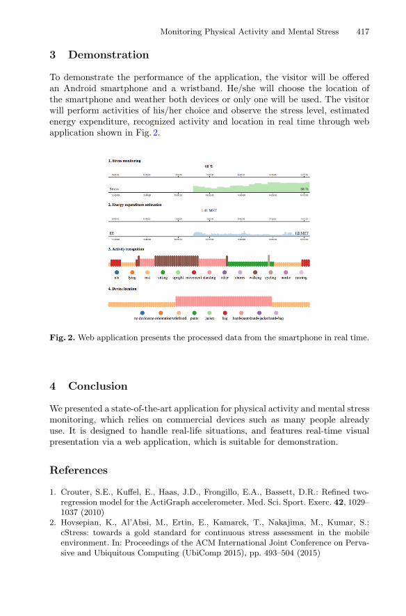
Monitoring Physical Activity and Mental Stress 417
3 Demonstration
To demonstrate the performance of the application, the visitor will be offeredan Android smartphone and a wristband. He/she will choose the location ofthe smartphone and weather both devices or only one will be used. The visitorwill perform activities of his/her choice and observe the stress level, estimatedenergy expenditure, recognized activity and location in real time through webapplication shown in Fig. 2.
Fig. 2. Web application presents the processed data from the smartphone in real time.
4 Conclusion
We presented a state-of-the-art application for physical activity and mental stressmonitoring, which relies on commercial devices such as many people alreadyuse. It is designed to handle real-life situations, and features real-time visualpresentation via a web application, which is suitable for demonstration.
References
1. Crouter, S.E., Kuffel, E., Haas, J.D., Frongillo, E.A., Bassett, D.R.: Refined two-regression model for the ActiGraph accelerometer. Med. Sci. Sport. Exerc. 42, 1029–1037 (2010)
2. Hovsepian, K., Al’Absi, M., Ertin, E., Kamarck, T., Nakajima, M., Kumar, S.:cStress: towards a gold standard for continuous stress assessment in the mobileenvironment. In: Proceedings of the ACM International Joint Conference on Perva-sive and Ubiquitous Computing (UbiComp 2015), pp. 493–504 (2015)

418 B. Cvetkovic et al.
3. Cvetkovic, B., Szeklicki, R., Janko, V., Lutomski, P., Lustrek, M.: Real-time activitymonitoring with a wristband and a smartphone. Inf. Fusion (2017)
4. Gjoreski, M., Gjoreski, H., Lustrek, M., Gams, M.: Continuous stress detection usinga wrist device: in laboratory and real life. In: UbiComp Adjunct, pp. 1185–1193(2016)
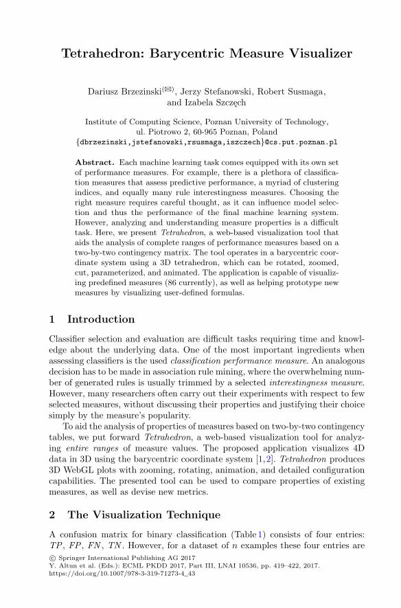
Tetrahedron: Barycentric Measure Visualizer
Dariusz Brzezinski(B), Jerzy Stefanowski, Robert Susmaga,and Izabela Szczech
Institute of Computing Science, Poznan University of Technology,ul. Piotrowo 2, 60-965 Poznan, Poland
{dbrzezinski,jstefanowski,rsusmaga,iszczech}@cs.put.poznan.pl
Abstract. Each machine learning task comes equipped with its own setof performance measures. For example, there is a plethora of classifica-tion measures that assess predictive performance, a myriad of clusteringindices, and equally many rule interestingness measures. Choosing theright measure requires careful thought, as it can influence model selec-tion and thus the performance of the final machine learning system.However, analyzing and understanding measure properties is a difficulttask. Here, we present Tetrahedron, a web-based visualization tool thataids the analysis of complete ranges of performance measures based on atwo-by-two contingency matrix. The tool operates in a barycentric coor-dinate system using a 3D tetrahedron, which can be rotated, zoomed,cut, parameterized, and animated. The application is capable of visualiz-ing predefined measures (86 currently), as well as helping prototype newmeasures by visualizing user-defined formulas.
1 Introduction
Classifier selection and evaluation are difficult tasks requiring time and knowl-edge about the underlying data. One of the most important ingredients whenassessing classifiers is the used classification performance measure. An analogousdecision has to be made in association rule mining, where the overwhelming num-ber of generated rules is usually trimmed by a selected interestingness measure.However, many researchers often carry out their experiments with respect to fewselected measures, without discussing their properties and justifying their choicesimply by the measure’s popularity.
To aid the analysis of properties of measures based on two-by-two contingencytables, we put forward Tetrahedron, a web-based visualization tool for analyz-ing entire ranges of measure values. The proposed application visualizes 4Ddata in 3D using the barycentric coordinate system [1,2]. Tetrahedron produces3D WebGL plots with zooming, rotating, animation, and detailed configurationcapabilities. The presented tool can be used to compare properties of existingmeasures, as well as devise new metrics.
2 The Visualization Technique
A confusion matrix for binary classification (Table 1) consists of four entries:TP , FP , FN , TN . However, for a dataset of n examples these four entries arec© Springer International Publishing AG 2017Y. Altun et al. (Eds.): ECML PKDD 2017, Part III, LNAI 10536, pp. 419–422, 2017.https://doi.org/10.1007/978-3-319-71273-4_43

420 D. Brzezinski et al.
Table 1. Confusion matrix for two-class classification
Fig. 1. Tetrahedron
sum-constrained, as n = TP+FP+FN +TN . Therefore, for a given constant n,any three values in the confusion matrix uniquely define the fourth value. Thisproperty allows to visualize any classification performance measure based on thetwo-class confusion matrix using a 4D barycentric coordinate system, tailored tosum-constrained data. The same holds for any 2 × 2 matrix, for example, thoseused to define rule interestingness measures [2].
The barycentric coordinate system is a coordinate system in which pointlocations are specified relatively to hyper-sides of a simplex. A 4D barycentriccoordinate system is a tetrahedron, where each dimension is represented as oneof the four vertices. Choosing vectors that represent TP , FP , FN , TN as verticesof a regular tetrahedron in a 3D space, one arrives at a barycentric coordinatesystem depicted in Fig. 1.
In this system, every confusion matrix [TP FNFP TN ] is represented as a point of
the tetrahedron. Let us illustrate this fact with a few examples. Figure 1 showsa skeleton of a tetrahedron with four exemplary points:
– one located in vertex TP, which represents [ n 00 0 ],
– one located in the middle of edge TP–FP, which represents[
n/2 0n/2 0
],
– one located in the middle of face �TP–FP–FN, which represents[
n/3 n/3n/3 0
],
– one located in the middle of the tetrahedron, which represents[
n/4 n/4n/4 n/4
].
One way of understanding this representation is to imagine a point in the tetra-hedron as the center of mass of the examples in a confusion matrix. If all nexamples are true positives, then the entire mass of the predictions is at TP andthe point coincides with vertex TP. If all examples are false negatives, the pointlies on vertex FN, etc. Generally, whenever a > b (a, b ∈ {TP ,FN ,FP ,TN })then the point is closer to the vertex corresponding to a rather than b.
Using the barycentric coordinate system makes it possible to depict the origi-nally 4D data (two-class confusion matrices) as points in 3D. Moreover, an addi-tional variable based on the depicted four values may be rendered as color. In thepresented tool, we adapt this procedure to color-code the values of classificationperformance and rule interestingness measures. A more in-depth description ofthe visualization and its possible applications can be found in [1,2].
Tetrahedron: Barycentric Measure Visualizer 421
3 Tool Overview
The described visualization technique has been implemented as an interactiveweb-based application. An online version, compatible with all modern web brow-sers across different client platforms, is publicly available1. The application canvisualize 86 predefined 4D measures, including 21 classification measures, 16rule interestingness measures, and 49 general-purpose formulas based on a two-by-two matrix. The user can also visualize custom measures by providing theirformula. The main functionalities of the application are:
– Interactive 3D tetrahedron visualization. The visualization (Fig. 2a)supports: 86 predefined measures, rotating, zooming, four rendering preci-sions, saving as an html with WebGL, and exporting images. The user maychoose to visualize external views, inner layers, and control point-padding.
– Cross-sections. A useful way of visualizing measure values can also beachieved be cutting the tetrahedron with a plane and analyzing the obtainedslice. In this application the user can visualize cross-sections (Fig. 2b) whichcorrespond to different class distributions. Interestingly, this particular kindof cross-sections produces a 2D space analogous to that used in ROC charts.
– Parameter animations. Several of the application options can be animated.These options can change the visualization parameters automatically in con-stant intervals creating an animation (Fig. 2c). Such animations can be use-ful when attempting to analyze: consecutive layers of the tetrahedron, the
Fig. 2. Application overview
1 https://dabrze.shinyapps.io/Tetrahedron/. Source codes at: https://github.com/dabrze/tetrahedron (MIT License).

422 D. Brzezinski et al.
Fig. 3. Visualizations of classification accuracy (Color figure online)
impact of measure parameters (e.g. the impact of β in Fβ-score), or the effectof changing class distributions on cross-sections.
– Custom measure definition. It is possible to define a custom measure tobe visualized by providing its formula (Fig. 2d).
Since classification accuracy is one of the most intuitive performance mea-sures, let us use it to exemplify visualizations produced by our tool with thedefault (blue: 0, red: 1) color map. One can notice that confusion matrices witha high number of FP and FN result in low accuracy (blue), whereas high TPand TN yield high accuracy (red). Cross-sections for two different class ratiosshow that on imbalanced data high accuracy can be achieved by trivial majorityclassifiers. More examples of visual-based analyses can be found in [1,2] (Fig. 3).
4 Conclusions
We propose Tetrahedron, a web-based visualization tool for analyzing and proto-typing measures based on a two-by-two matrix. Its main features include: inter-active 3D WebGL barycentric plots, zooming, parameter animation, performingcross-sections, providing custom measure formulas, and saving plots with a singleclick. Such functionality facilitates visual inspection of various measure proper-ties, such as determining measure monotonicity, symmetries, maximas, or unde-fined values. Thus, the presented tool can be used to gain further understandingof existing machine learning measures, as well as devise new ones.
Acknowledgments. NCN DEC-2013/11/B/ST6/00963, PUT Statutory Funds.
References
1. Brzezinski, D., Stefanowski, J., Susmaga, R., Szczech, I.: Visual-based analysis ofclassification measures with applications to imbalanced data. arXiv:1704.07122
2. Susmaga, R., Szczech, I.: Can interestingness measures be usefully visualized? Int.J. Appl. Math. Comp. Sci. 25(2), 323–336 (2015)
TF Boosted Trees: A Scalable TensorFlowBased Framework for Gradient Boosting
Natalia Ponomareva1(B), Soroush Radpour2, Gilbert Hendry3, Salem Haykal2,Thomas Colthurst3, Petr Mitrichev4, and Alexander Grushetsky2
1 Google, Inc., New York, [email protected]
2 Google, Inc., Mountain View, USA3 Google, Inc., Cambridge, USA
4 Google, Inc., Zurich, Switzerland
Abstract. TF Boosted Trees (TFBT) is a new open-sourced frame-work for the distributed training of gradient boosted trees. It is basedon TensorFlow, and its distinguishing features include a novel architec-ture, automatic loss differentiation, layer-by-layer boosting that results insmaller ensembles and faster prediction, principled multi-class handling,and a number of regularization techniques to prevent overfitting.
Keywords: Distributed gradient boosting · TensorFlow
1 Introduction
Gradient boosted trees are popular machine learning models. Since their intro-duction in [3] they have gone on to dominate many competitions on real-worlddata, including Kaggle and KDDCup [2]. In addition to their excellent accuracy,they are also easy to use, as they deal well with unnormalized, collinear, missing,or outlier-infected data. They can support custom loss functions and are ofteneasier to interpret than neural nets or large linear models. Because of their pop-ularity, there are now many gradient boosted tree implementations, includingscikit-learn [7], R gbm [8], Spark MLLib [5], LightGBM [6], XGBoost [2].
In this paper, we introduce another optimized and scalable gradient boostedtree library, TF Boosted Trees (TFBT), which is built on top of theTensorFlow framework [1]. TFBT incorporates a number of novel algorith-mic improvements to the gradient boosting algorithm, including new per-layer boosting procedure which offers improved performance on some problems.TFBT is open source, and available in the main TensorFlow distribution undercontrib/boosted trees.
2 TFBT Features
In Table 1 we provide a brief comparison between TFBT and some existinglibraries. Additionally, TFBT provides the following.c© Springer International Publishing AG 2017Y. Altun et al. (Eds.): ECML PKDD 2017, Part III, LNAI 10536, pp. 423–427, 2017.https://doi.org/10.1007/978-3-319-71273-4_44
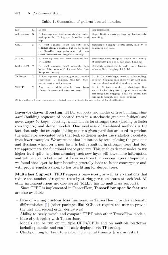
424 N. Ponomareva et al.
Table 1. Comparison of gradient boosted libraries.
Lib D? Losses Regularization
scikit-learn N R: least squares, least absolute dev, huber
and quantile. C : logistic, Max-Ent and
exp
Depth limit, shrinkage, bagging, feature sub-
sampling
GBM N R: least squares, least absolute dev,
t-distribution, quantile, huber. C : logis-
tic, Max-Ent, exp, poisson & right cen-
sored observations. Supports ranking
Shrinkage, bagging, depth limit, min # of
examples per node
MLLib Y R: least squared and least absolute dev.
C : logistic
Shrinkage, early stopping, depth limit, min #
of examples per node, min gain, bagging
Light GBM Y R: least squares, least absolute dev,
huber, fair, poisson. C : logistic, Max-Ent.
Supports ranking
Dropout, shrinkage, # leafs limit, feature
subsampling, bagging, L1 & L2
XGBoost Y R: least squares, poisson, gamma, tweedie
regression. C : logistic, Max-Ent. Sup-
ports ranking and custom
L1 & L2, shrinkage, feature subsampling,
dropout, bagging, min child weight and gain,
limit on depth and # of nodes, pruning
TFBT Y Any twice differentiable loss from
tf.contrib.losses and custom losses
L1 & L2, tree complexity, shrinkage, line
search for learning rate, dropout, feature sub-
sampling and bagging, limit on depth and
min node weight, pre- post- pruning
D? is whether a library supports distributed mode. R stands for regression, C for classification.
Layer-by-Layer Boosting. TFBT supports two modes of tree building: stan-dard (building sequence of boosted trees in a stochastic gradient fashion) andnovel Layer-by-Layer boosting, which allows for stronger trees (leading to fasterconvergence) and deeper models. One weakness of tree-based methods is thefact that only the examples falling under a given partition are used to producethe estimator associated with that leaf, so deeper nodes use statistics calculatedfrom fewer examples. We overcome that limitation by recalculating the gradientsand Hessians whenever a new layer is built resulting in stronger trees that bet-ter approximate the functional space gradient. This enables deeper nodes to usehigher level splits as priors meaning each new layer will have more informationand will be able to better adjust for errors from the previous layers. Empiricallywe found that layer-by-layer boosting generally leads to faster convergence and,with proper regularization, to less overfitting for deeper trees.
Multiclass Support. TFBT supports one-vs-rest, as well as 2 variations thatreduce the number of required trees by storing per-class scores at each leaf. Allother implementations use one-vs-rest (MLLib has no multiclass support).
Since TFBT is implemented in TensorFlow, TensorFlow specific featuresare also available
– Ease of writing custom loss functions, as TensorFlow provides automaticdifferentiation [1] (other packages like XGBoost require the user to providethe first and second order derivatives).
– Ability to easily switch and compare TFBT with other TensorFlow models.– Ease of debugging with TensorBoard.– Models can be run on multiple CPUs/GPUs and on multiple platforms,
including mobile, and can be easily deployed via TF serving.– Checkpointing for fault tolerance, incremental training & warm restart.
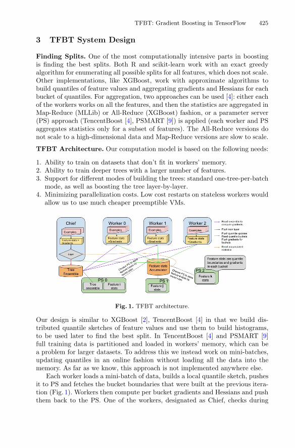
TFBT: Gradient Boosting in TensorFlow 425
3 TFBT System Design
Finding Splits. One of the most computationally intensive parts in boostingis finding the best splits. Both R and scikit-learn work with an exact greedyalgorithm for enumerating all possible splits for all features, which does not scale.Other implementations, like XGBoost, work with approximate algorithms tobuild quantiles of feature values and aggregating gradients and Hessians for eachbucket of quantiles. For aggregation, two approaches can be used [4]: either eachof the workers works on all the features, and then the statistics are aggregated inMap-Reduce (MLLib) or All-Reduce (XGBoost) fashion, or a parameter server(PS) approach (TencentBoost [4], PSMART [9]) is applied (each worker and PSaggregates statistics only for a subset of features). The All-Reduce versions donot scale to a high-dimensional data and Map-Reduce versions are slow to scale.
TFBT Architecture. Our computation model is based on the following needs:
1. Ability to train on datasets that don’t fit in workers’ memory.2. Ability to train deeper trees with a larger number of features.3. Support for different modes of building the trees: standard one-tree-per-batch
mode, as well as boosting the tree layer-by-layer.4. Minimizing parallelization costs. Low cost restarts on stateless workers would
allow us to use much cheaper preemptible VMs.
Fig. 1. TFBT architecture.
Our design is similar to XGBoost [2], TencentBoost [4] in that we build dis-tributed quantile sketches of feature values and use them to build histograms,to be used later to find the best split. In TencentBoost [4] and PSMART [9]full training data is partitioned and loaded in workers’ memory, which can bea problem for larger datasets. To address this we instead work on mini-batches,updating quantiles in an online fashion without loading all the data into thememory. As far as we know, this approach is not implemented anywhere else.
Each worker loads a mini-batch of data, builds a local quantile sketch, pushesit to PS and fetches the bucket boundaries that were built at the previous itera-tion (Fig. 1). Workers then compute per bucket gradients and Hessians and pushthem back to the PS. One of the workers, designated as Chief, checks during

426 N. Ponomareva et al.
Algorithm 1. Chief and Workers’ work1: procedure CalculateStatistics(ps, model, stamp, batch data, loss fn)2: predictions ← model.predict(BATCH DATA)3: quantile stats ← calculate quantile stats(BATCH DATA)4: push stats(PS,quantile stats, stamp) � PS updates quantiles5: current boundaries ← fetch latest boundaries(PS, stamp)6: gradients, hessians ← calculate derivatives(predictions,LOSS FN)7: gradients, hessians ← aggregate(current boundaries,gradients, hessians)8: push stats(PS,gradients, hessians, size(BATCH DATA), stamp)
9: procedure DoWork(ps, loss fn, is chief) � Runs on workers and 1 chief10: while true do11: BATCH DATA ← read data batch()12: model ← fetch latest model(PS)13: stamp ← model.stamp token14: CalculateStatistics(PS,model, stamp, BATCH DATA,LOSS FN)15: if is chief & get num examples(PS, stamp) ≥ N PER LAY ER then16: next stamp ← stamp + 117: stats ← flush(PS, stamp, next stamp) � Update stamp, returns stats18: build layer(PS, model, next stamp, stats) � PS updates ensemble
each iteration if the PS have accumulated enough statistics for the current layerand if so, starts building the new layer by finding best splits for each of thenodes in the layer. Code that finds the best splits for each feature is executed onthe PS that have accumulated the gradient statistics for the feature. The Chiefreceives the best split for every leaf from the PS and grows a new layer on thetree.
Once the Chief adds a new layer, both gradients and quantiles become stale.To avoid stale updates, we introduce an abstraction called StampedResource -a TensorFlow resource with an int64 stamp. Tree ensemble, as well as gradientsand quantile accumulators are all stamped resources with such token. When theworker fetches the model, it gets the stamp token which is then used for allthe reads and writes to stamped resources until the end of the iteration. Thisguarantees that all the updates are consistent and ensures that Chief doesn’tneed to wait for Workers for synchronization, which is important when usingpreemptible VMs. Chief checkpoints resources to disk and workers don’t holdany state, so if they are restarted, they can load a new mini-batch and continue.
References
1. Abadi, M., et al.: TensorFlow: large-scale machine learning on heterogeneous dis-tributed systems. In: OSDI (2016)
2. Chen, T., et al.: XGBoost: a scalable tree boosting system. CoRR (2016)3. Friedman, J.H.: Greedy function approximation: a gradient boosting machine. Ann.
Stat. 29, 1189–1232 (2000)4. Jiang, J., Jiang, J., Cui, B., Zhang, C.: TencentBoost: a gradient boosting tree sys-
tem with parameter server. In: 33rd IEEE International Conference on Data Engi-neering, ICDE 2017, San Diego, CA, USA, 19–22 April 2017, pp. 281–284 (2017).https://doi.org/10.1109/ICDE.2017.87

TFBT: Gradient Boosting in TensorFlow 427
5. Meng, X., Bradley, J.K., Yavuz, B., Sparks, E.R., Venkataraman, S., Liu, D., Free-man, J., Tsai, D.B., Amde, M., Owen, S., Xin, D., Xin, R., Franklin, M.J., Zadeh,R., Zaharia, M., Talwalkar, A.: MLlib: machine learning in Apache Spark. CoRR(2015). http://arxiv.org/abs/1505.06807
6. Microsoft: Microsoft/dmtk (2013). https://github.com/microsoft/dmtk7. Pedregosa, F., Varoquaux, G., Gramfort, A., Michel, V., Thirion, B., Grisel, O.,
Blondel, M., Prettenhofer, P., Weiss, R., Dubourg, V., Vanderplas, J., Passos, A.,Cournapeau, D., Brucher, M., Perrot, M., Duchesnay, E.: Scikit-learn: machinelearning in Python. J. Mach. Learn. Res. 12, 2825–2830 (2011)
8. Ridgeway, G.: Generalized boosted models: a guide to the GBM package (2005)9. Zhou, J., et al.: PSMART: parameter server based multiple additive regression trees
system. In: WWW 2017 Companion (2017)
TrajViz: A Tool for Visualizing Patternsand Anomalies in Trajectory
Yifeng Gao(B), Qingzhe Li, Xiaosheng Li, Jessica Lin, and Huzefa Rangwala
George Mason University, Fairfax, USA{ygao12,qli10,xli22,jessica}@gmu.edu, [email protected]
Abstract. Visualizing frequently occurring patterns and potentiallyunusual behaviors in trajectory can provide valuable insights into activ-ities behind the data. In this paper, we introduce TrajViz, a motif (fre-quently repeated subsequences) based visualization software that detectspatterns and anomalies by inducing “grammars” from discretized spa-tial trajectories. We consider patterns as a set of sub-trajectories withunknown lengths that are spatially similar to each other. We demon-strate that TrajViz has the capacity to help users visualize anomaliesand patterns effectively.
1 Introduction
With the rapid growth of tracking technology, a large amount of trajectory dataare generated from users’ daily activities. Discovering frequently occurring pat-terns (motifs) and potentially unusual behaviors can be used to summarize theoverwhelming amount of trajectories data and obtain meaningful knowledge. Inthis paper, we present TrajViz, a software that visualizes patterns and anomaliesin trajectory datasets. TrajViz extends our previous work in time series motifdiscovery [1] to sub-trajectory pattern visualization. We consider patterns as aset of sub-trajectories with unknown lengths that are spatially similar to eachother. We use a grid-based discretization approach to remove the speed informa-tion and adapt a grammar-based motif discovery algorithm, Iterative Sequitur(ItrSequitur), to discover the patterns. We design a user-friendly interface toallow visualization of repeated, as well as unusual sub-trajectories within thedatasets.
2 Relate Work and Overview of TrajViz
Previously, we introduced a grammar-based motif discovery framework [7], whichuses Sequitur [4], a grammar induction algorithm, to find approximate motifsof variable lengths in time series. However, the unique characteristics and chal-lenges associated with spatial trajectory data make it unsuitable and difficult toapply the algorithms directly on trajectory data. In [5], the authors introducedSTAVIS, a trajectory analytical system that uses grammar induction to infervariable-length patterns. However, its definition of “pattern” is based on timec© Springer International Publishing AG 2017Y. Altun et al. (Eds.): ECML PKDD 2017, Part III, LNAI 10536, pp. 428–431, 2017.https://doi.org/10.1007/978-3-319-71273-4_45
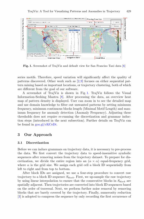
TrajViz: A Tool for Visualizing Patterns and Anomalies in Trajectory 429
Fig. 1. Screenshot of TrajViz and default view for San Franciso Taxi data [6]
series motifs. Therefore, speed variation will significantly affect the quality ofpatterns discovered. Other work such as [2,9] focuses on either sequential pat-tern mining based on important locations, or trajectory clustering, both of whichare different from the goal of our software.
A screenshot of TrajViz is shown in Fig. 1. TrajViz follows the VisualInformation-Seeking Mantra [8]. After processing the data, an overview heatmap of pattern density is displayed. User can zoom in to see the detailed mapand use domain knowledge to filter out unwanted patterns by setting minimumfrequency, minimum continuous blocks length (Minimal Motif Length) and max-imum frequency for anomaly detection (Anomaly Frequency). Adjusting thesethresholds does not require re-running the discretization and grammar induc-tion steps (introduced in the next subsection). Further details on TrajViz canbe found in goo.gl/cKCeDt.
3 Our Approach
3.1 Discretization
Before we can induce grammars on trajectory data, it is necessary to pre-processthe data. We first convert the trajectory data to speed-insensitive symbolicsequences after removing noises from the trajectory dataset. To prepare for dis-cretization, we divide the entire region into an (α × α) equal-frequency grid,where α is the grid size. We assign each grid cell a block ID sequentially fromleft to right and from top to bottom.
After block IDs are assigned, we use a four-step procedure to convert rawtrajectory to a block ID sequence Sblock. First, we up-sample the raw trajectoryby using linear interpolation to ensure that the consecutive blocks in Sblock arespatially adjacent. Then trajectories are converted into block ID sequences basedon the order of traversal. Next, we perform further noise removal by removingblocks that are barely covered by the trajectory. Finally, numerosity reduction[3] is adopted to compress the sequence by only recording the first occurrence of
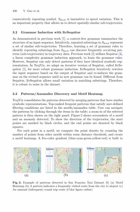
430 Y. Gao et al.
consecutively repeating symbol. Sblock is insensitive to speed variation. This isan important property that allows us to detect spatially-similar sub-trajectories.
3.2 Grammar Induction with ItrSequitur
As demonstrated in previous work [7], a context-free grammar summarizes thestructure of an input sequence. Intuitively, repeated substrings in Sblock representa set of similar sub-trajectories. Therefore, learning a set of grammar rules toidentify repeating substrings from Sblock can discover frequently occurring pat-terns (sub-trajectories) in trajectory data. Previous work [5] utilizes Sequitur [4],a linear complexity grammar induction approach, to learn the grammar rules.However, Sequitur can only detect patterns if they have identical symbolic rep-resentation. In TrajViz, we adapt an iterative version of Sequitur, called ItrSe-quitur [1], for more robust grammar induction. ItrSequitur iteratively rewritesthe input sequence based on the output of Sequitur and re-induces the gram-mar on the revised sequence until no new grammar can be found. Different fromSequitur, ItrSequitur allows small variation in matching substrings. Therefore,it is robust to noise in the dataset.
3.3 Patterns/Anomalies Discovery and Motif Heatmap
TrajViz consolidates the patterns detected by merging patterns that have similarsymbolic representations. Top-ranked frequent patterns that satisfy user-definedfiltering conditions are listed in the motifs/anomalies table. User can navigatethe patterns by clicking through the items in the table; a zoom-in of the selectedpattern is then shown on the right panel. Figure 2 shows screenshots of a motifand an anomaly detected. To show the direction of the trajectories, the startpoints are marked by black circles, and the end points are denoted by blacksquares.
For each point in a motif, we compute the point density by counting thenumber of points from other motifs within some distance threshold, and createa motif heatmap. A five-color gradient (blue-cyan-green-yellow-red) is built to
Fig. 2. Example of patterns detected in San Franciso Taxi Dataset [6] (a) MotifHeatmap (b) A pattern indicates a frequently visited route from the city to airport (c)An unusual (infrequent) round trip route (Color figure online)
TrajViz: A Tool for Visualizing Patterns and Anomalies in Trajectory 431
linearly map the densities to their specific colors. The most dense points havethe red colors while the least dense ones are in blue.
To find anomalies, we create a trajectory rule-density curve by counting thenumber of grammar rules covering each consecutive pair of block IDs (we considera pair at a time in order to preserve the direction of the trajectory). The intuitionis that, an anomalous subsequence would have zero or very few repetitions, hencelow rule-density. TrajViz finds low-density subsequences within a trajectory andmarks them as unusual routes (Fig. 2(c)).
4 Target Audience
TrajViz provides an efficient, interpretable, and user-interactive mechanism tounderstand functional activities behind massive trajectory data. TrajViz targetsa diverse audience including researchers, practitioners, and scientists who areinterested in discovering patterns in trajectory data.
Acknowledgements. We would like to thank Ranjeev Mittu at the Naval ResearchLab (NRL) for the support and valuable suggestions on our work.
References
1. Gao, Y., Lin, J., Rangwala, H.: Iterative grammar-based framework for discoveringvariable-length time series motifs. In: 2016 15th IEEE International Conference onMachine Learning and Applications (ICMLA), pp. 7–12. IEEE (2016)
2. Lee, J.-G., Han, J., Li, X., Gonzalez, H.: Traclass: trajectory classification usinghierarchical region-based and trajectory-based clustering. Proc. VLDB Endow. 1(1),1081–1094 (2008)
3. Lin, J., Keogh, E., Wei, L., Lonardi, S.: Experiencing sax: a novel symbolic repre-sentation of time series. Data Min. Knowl. Disc. 15(2), 107–144 (2007)
4. Nevill-Manning, C.G., Witten, I.H.: Identifying hierarchical strcture in sequences:a linear-time algorithm. J. Artif. Intell. Res. (JAIR) 7, 67–82 (1997)
5. Oates, T., Boedihardjo, A.P., Lin, J., Chen, C., Frankenstein, S., Gandhi, S.: Motifdiscovery in spatial trajectories using grammar inference. In: Proceedings of the22nd ACM International Conference on Conference on Information & KnowledgeManagement, pp. 1465–1468. ACM (2013)
6. Piorkowski, M., Sarafijanovic-Djukic, N., Grossglauser, M.: A parsimonious modelof mobile partitioned networks with clustering. In: 2009 First International Com-munication Systems and Networks and Workshops, pp. 1–10. IEEE (2009)
7. Senin, P., Lin, J., Wang, X., Oates, T., Gandhi, S., Boedihardjo, A.P., Chen, C.,Frankenstein, S., Lerner, M.: GrammarViz 2.0: a tool for grammar-based patterndiscovery in time series. In: Calders, T., Esposito, F., Hullermeier, E., Meo, R. (eds.)ECML PKDD 2014. LNCS (LNAI), vol. 8726, pp. 468–472. Springer, Heidelberg(2014). https://doi.org/10.1007/978-3-662-44845-8 37
8. Shneiderman, B.: The eyes have it: a task by data type taxonomy for informationvisualizations. In: IEEE Symposium on Visual Languages, 1996. Proceedings, pp.336–343. IEEE (1996)
9. Zheng, Y., Zhang, L., Xie, X., Ma, W.-Y.: Mining interesting locations and travelsequences from GPS trajectories. In: Proceedings of the 18th International Confer-ence on World Wide Web, pp. 791–800. ACM (2009)

TrAnET: Tracking and Analyzing the Evolutionof Topics in Information Networks
Livio Bioglio, Ruggero G. Pensa(B) , and Valentina Rho
Department of Computer Science, University of Turin, Turin, Italy{livio.bioglio,ruggero.pensa,valentina.rho}@unito.it
Abstract. This paper presents a system for tracking and analyzing theevolution and transformation of topics in an information network. Thesystem consists of four main modules for pre-processing, adaptive topicmodeling, network creation and temporal network analysis. The coremodule is built upon an adaptive topic modeling algorithm adoptinga sliding time window technique that enables the discovery of ground-breaking ideas as those topics that evolve rapidly in the network.
Keywords: Information diffusion · Topic modelingCitation networks
1 Introduction
Information diffusion is an important and widely-studied topic in computa-tional social science and network analytics due to its applications to socialmedia/network analysis, viral marketing campaigns, influence maximization andprediction. An information diffusion process takes place when some nodes (e.g.,customers, social profiles, scientific authors) influence some of their neighbors inthe network which, in their turn, influence some of their respective neighbors.The definition of “influence” depends on the application. In mouth-to-mouthviral campaign, a user who bought a product at time t influence their neighborsif they buy the same product at time t + δ. In bibliographic networks, author ainfluences author b when a and b are connected by some relationship (e.g., col-laboration, co-authorship, citation) and either b cites one of the papers publishedby author a, or author b publish in the same topic as author a [2].
In this paper we propose a system for topic diffusion analysis based on adaptiveand scalable Latent Dirichlet Annotation (LDA [1]) that uses a different notion ofinfluence: for a given topic x, author a influences author b when b publish at timet + δ a paper that cites some papers covering topic x and authored by a at timet. Moreover, our focus is on topic evolution rather than on ranking authors, suchas in [5]. Our system, in fact, enables the discovery of groundbreaking topics andideas, which are defined as topics that evolve rapidly in the network. Accordingto our definition, the most interesting topics are those that influence many newresearch topics, thus stimulating new research ideas. By setting different diffusionc© Springer International Publishing AG 2017Y. Altun et al. (Eds.): ECML PKDD 2017, Part III, LNAI 10536, pp. 432–436, 2017.https://doi.org/10.1007/978-3-319-71273-4_46
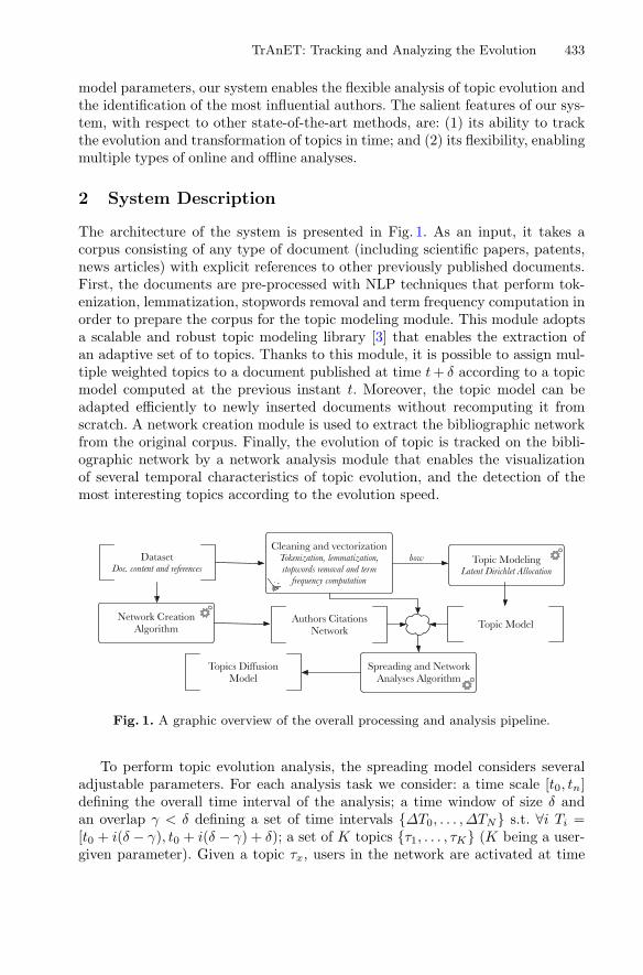
TrAnET: Tracking and Analyzing the Evolution 433
model parameters, our system enables the flexible analysis of topic evolution andthe identification of the most influential authors. The salient features of our sys-tem, with respect to other state-of-the-art methods, are: (1) its ability to trackthe evolution and transformation of topics in time; and (2) its flexibility, enablingmultiple types of online and offline analyses.
2 System Description
The architecture of the system is presented in Fig. 1. As an input, it takes acorpus consisting of any type of document (including scientific papers, patents,news articles) with explicit references to other previously published documents.First, the documents are pre-processed with NLP techniques that perform tok-enization, lemmatization, stopwords removal and term frequency computation inorder to prepare the corpus for the topic modeling module. This module adoptsa scalable and robust topic modeling library [3] that enables the extraction ofan adaptive set of to topics. Thanks to this module, it is possible to assign mul-tiple weighted topics to a document published at time t + δ according to a topicmodel computed at the previous instant t. Moreover, the topic model can beadapted efficiently to newly inserted documents without recomputing it fromscratch. A network creation module is used to extract the bibliographic networkfrom the original corpus. Finally, the evolution of topic is tracked on the bibli-ographic network by a network analysis module that enables the visualizationof several temporal characteristics of topic evolution, and the detection of themost interesting topics according to the evolution speed.
Fig. 1. A graphic overview of the overall processing and analysis pipeline.
To perform topic evolution analysis, the spreading model considers severaladjustable parameters. For each analysis task we consider: a time scale [t0, tn]defining the overall time interval of the analysis; a time window of size δ andan overlap γ < δ defining a set of time intervals {ΔT0, . . . ,ΔTN} s.t. ∀i Ti =[t0 + i(δ − γ), t0 + i(δ − γ) + δ); a set of K topics {τ1, . . . , τK} (K being a user-given parameter). Given a topic τx, users in the network are activated at time

434 L. Bioglio et al.
ΔT0 if they publish a paper covering topic τx during ΔT0. Users are activated attime ΔTi (i > 0) if they cite any paper that contributed to the activation of theusers at time ΔTi−1. A paper p is said to cover a topic τx if LDA has assignedτx to paper p with a weight greater than a user-specified threshold.
The whole process is driven within an interactive Jupyter notebook1. Allmodules are implemented in Python. All data are stored in a MongoDB2
database server. The system runs on Windows, Linux and Mac OS X oper-ating systems using a standard computing platform (e.g., any multi-core IntelCore iX CPU, and 8 GB RAM) and does not require any high-performance GPUarchitecture.
3 Demonstration
Dataset. The dataset used for TrAnET demonstration is a subset of the scien-tific papers citations network. This dataset is created by automatically mergingtwo datasets originally extracted through ArnetMiner [4]: the DBLP and ACMcitation networks3. The demonstration focuses on papers published from 2000to 2014 within a set of preselected venues, for a total of about 155,000 papers.
Text Processing and Topic Extraction. The input data given to the topicextraction module is obtained as the result of the cleaning and vectorizationprocess performed on the concatenation of paper title and abstract, as describedin the previous section. In particular, the cleaning module ignores terms thatappears only once in the dataset and in more than 80% of the documents. Thetopic extraction is performed on the whole dataset using Latent Dirichlet Alloca-tion, searching for 50 topics. The topic model is then used to assign a weightedlist of topics to each paper in the dataset. In our demonstration, we consideronly topic assignments with weight greater than 0.2.
Example of Topic Evolution. To explain how our tool works, the analysison two representative topics (namely, topics 6 and 34) is shown here: their key-words, sized according to their weight within the topic, are described in Fig. 2aand b, respectively. These topics have been chosen because they are assignedto a comparable number of papers (4498 for topic 6 and 6079 for topic 34)and authors (8430 for topic 6 and 8776 for topic 34). Moreover, they exhibit avery similar publication trend. According to Fig. 2c, which shows the cumulativenumber of authors that have published for the first time a paper on each topicin each year, the two trends are almost indistinguishable. This result (similar towhat can be computed by [2]) shows that these topics have a similar diffusiontrend in the bibliographic network. However, there is a strong difference in theevolution speed, as shown in Fig. 2d. Topic 34 (information retrieval) evolves1 https://jupyter.org/.2 https://www.mongodb.com/.3 https://aminer.org/citation.
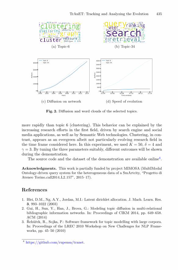
TrAnET: Tracking and Analyzing the Evolution 435
(a) Topic-6 (b) Topic-34
(c) Diffusion on network (d) Speed of evolution
Fig. 2. Diffusion and word clouds of the selected topics.
more rapidly than topic 6 (clustering). This behavior can be explained by theincreasing research efforts in the first field, driven by search engine and socialmedia applications, as well as by Semantic Web technologies. Clustering, in con-trast, appears as an evergreen albeit not particularly evolving research field inthe time frame considered here. In this experiment, we used K = 50, δ = 4 andγ = 3. By tuning the three parameters suitably, different outcomes will be shownduring the demonstration.
The source code and the dataset of the demonstration are available online4.
Acknowledgments. This work is partially funded by project MIMOSA (MultIModalOntology-driven query system for the heterogeneous data of a SmArtcity, “Progetto diAteneo Torino call2014 L2 157”, 2015–17).
References
1. Blei, D.M., Ng, A.Y., Jordan, M.I.: Latent dirichlet allocation. J. Mach. Learn. Res.3, 993–1022 (2003)
2. Gui, H., Sun, Y., Han, J., Brova, G.: Modeling topic diffusion in multi-relationalbibliographic information networks. In: Proceedings of CIKM 2014, pp. 649–658.ACM (2014)
3. Rehurek, R., Sojka, P.: Software framework for topic modelling with large corpora.In: Proceedings of the LREC 2010 Workshop on New Challenges for NLP Frame-works, pp. 45–50 (2010)
4 https://github.com/rupensa/tranet.

436 L. Bioglio et al.
4. Tang, J., Zhang, J., Yao, L., Li, J., Zhang, L., Su, Z.: ArnetMiner: extraction andmining of academic social networks. In: KDD 2008, pp. 990–998 (2008)
5. Xiong, C., Power, R., Callan, J.: Explicit semantic ranking for academic search viaknowledge graph embedding. In: Proceedings of WWW 2017, pp. 1271–1279. ACM(2017)
WHODID: W eb-Based Interfacefor Human-Assisted Factory Operations
in Fault Detection, Identification and Diagnosis
Pierre Blanchart(B) and Cedric Gouy-Pailler
CEA, LIST, 91191 Gif-sur-Yvette Cedex, [email protected]
Abstract. We present WHODID: a turnkey intuitive web-based inter-face for fault detection, identification and diagnosis in production units.Fault detection and identification is an extremely useful feature and isbecoming a necessity in modern production units. Moreover, the largedeployment of sensors within the stations of a production line has enabledthe close monitoring of products being manufactured. In this context,there is a high demand for computer intelligence able to detect and isolatefaults inside production lines, and to additionally provide a diagnosis formaintenance on the identified faulty production device, with the purposeof preventing subsequent faults caused by the diagnosed faulty devicebehavior. We thus introduce a system which has fault detection, isola-tion, and identification features, for retrospective and on-the-fly moni-toring and maintenance of complex dynamical production processes. Itprovides real-time answers to the questions: “is there a fault?”, “wheredid it happen?”, “for what reason?”. The method is based on a posteriorianalysis of decision sequences in XGBoost tree models, using recurrentneural networks sequential models of tree paths.
The particularity of the presented system is that it is robust to miss-ing or faulty sensor measurements, it does not require any modeling ofthe underlying, possibly exogenous manufacturing process, and providesfault diagnosis along with confidence level in plain English formulations.The latter can be used as maintenance directions by a human operatorin charge of production monitoring and control.
Keywords: Production units · Fault detection and identificationMaintenance operator friendly · Tree ensemble · Gradient boostingLSTM-RNN networks
1 Introduction
Modern factories operation and optimization rely on fine-grained monitoring ofmachines and products. Besides classical purposes such as energy optimizationand smart production planning, there is a high demand for systems able to detectand isolate the location of faults occurring in production chains. Thus there hasc© Springer International Publishing AG 2017Y. Altun et al. (Eds.): ECML PKDD 2017, Part III, LNAI 10536, pp. 437–441, 2017.https://doi.org/10.1007/978-3-319-71273-4_47
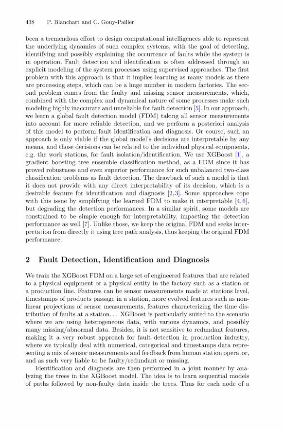
438 P. Blanchart and C. Gouy-Pailler
been a tremendous effort to design computational intelligences able to representthe underlying dynamics of such complex systems, with the goal of detecting,identifying and possibly explaining the occurrence of faults while the system isin operation. Fault detection and identification is often addressed through anexplicit modeling of the system processes using supervised approaches. The firstproblem with this approach is that it implies learning as many models as thereare processing steps, which can be a huge number in modern factories. The sec-ond problem comes from the faulty and missing sensor measurements, which,combined with the complex and dynamical nature of some processes make suchmodeling highly inaccurate and unreliable for fault detection [5]. In our approach,we learn a global fault detection model (FDM) taking all sensor measurementsinto account for more reliable detection, and we perform a posteriori analysisof this model to perform fault identification and diagnosis. Or course, such anapproach is only viable if the global model’s decisions are interpretable by anymeans, and those decisions can be related to the individual physical equipments,e.g. the work stations, for fault isolation/identification. We use XGBoost [1], agradient boosting tree ensemble classification method, as a FDM since it hasproved robustness and even superior performance for such unbalanced two-classclassification problems as fault detection. The drawback of such a model is thatit does not provide with any direct interpretability of its decision, which is adesirable feature for identification and diagnosis [2,3]. Some approaches copewith this issue by simplifying the learned FDM to make it interpretable [4,6],but degrading the detection performances. In a similar spirit, some models areconstrained to be simple enough for interpretability, impacting the detectionperformance as well [7]. Unlike those, we keep the original FDM and seeks inter-pretation from directly it using tree path analysis, thus keeping the original FDMperformance.
2 Fault Detection, Identification and Diagnosis
We train the XGBoost FDM on a large set of engineered features that are relatedto a physical equipment or a physical entity in the factory such as a station ora production line. Features can be sensor measurements made at stations level,timestamps of products passage in a station, more evolved features such as non-linear projections of sensor measurements, features characterizing the time dis-tribution of faults at a station. . . XGBoost is particularly suited to the scenariowhere we are using heterogeneous data, with various dynamics, and possiblymany missing/abnormal data. Besides, it is not sensitive to redundant features,making it a very robust approach for fault detection in production industry,where we typically deal with numerical, categorical and timestamps data repre-senting a mix of sensor measurements and feedback from human station operator,and as such very liable to be faulty/redundant or missing.
Identification and diagnosis are then performed in a joint manner by ana-lyzing the trees in the XGBoost model. The idea is to learn sequential modelsof paths followed by non-faulty data inside the trees. Thus for each node of a
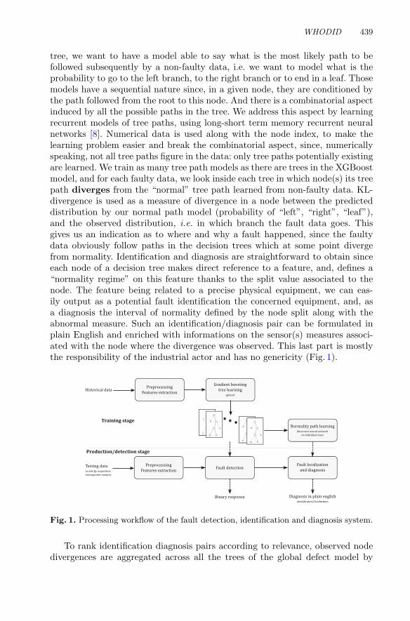
WHODID 439
tree, we want to have a model able to say what is the most likely path to befollowed subsequently by a non-faulty data, i.e. we want to model what is theprobability to go to the left branch, to the right branch or to end in a leaf. Thosemodels have a sequential nature since, in a given node, they are conditioned bythe path followed from the root to this node. And there is a combinatorial aspectinduced by all the possible paths in the tree. We address this aspect by learningrecurrent models of tree paths, using long-short term memory recurrent neuralnetworks [8]. Numerical data is used along with the node index, to make thelearning problem easier and break the combinatorial aspect, since, numericallyspeaking, not all tree paths figure in the data: only tree paths potentially existingare learned. We train as many tree path models as there are trees in the XGBoostmodel, and for each faulty data, we look inside each tree in which node(s) its treepath diverges from the “normal” tree path learned from non-faulty data. KL-divergence is used as a measure of divergence in a node between the predicteddistribution by our normal path model (probability of “left”, “right”, “leaf”),and the observed distribution, i.e. in which branch the fault data goes. Thisgives us an indication as to where and why a fault happened, since the faultydata obviously follow paths in the decision trees which at some point divergefrom normality. Identification and diagnosis are straightforward to obtain sinceeach node of a decision tree makes direct reference to a feature, and, defines a“normality regime” on this feature thanks to the split value associated to thenode. The feature being related to a precise physical equipment, we can eas-ily output as a potential fault identification the concerned equipment, and, asa diagnosis the interval of normality defined by the node split along with theabnormal measure. Such an identification/diagnosis pair can be formulated inplain English and enriched with informations on the sensor(s) measures associ-ated with the node where the divergence was observed. This last part is mostlythe responsibility of the industrial actor and has no genericity (Fig. 1).
Fig. 1. Processing workflow of the fault detection, identification and diagnosis system.
To rank identification diagnosis pairs according to relevance, observed nodedivergences are aggregated across all the trees of the global defect model by
440 P. Blanchart and C. Gouy-Pailler
computing in which proportion an individual tree score contributes to the globaldefect score and reweighing accordingly. It enables a ranking of potential faultdiagnosis by decreasing order of relevance. This human readable output thenallows an operator in charge of production chain maintenance and control toaddress the problem in the right place.
3 Interface Operation
The interface operation is demonstrated in Fig. 2: the operator selects a produc-tion line in the hierarchical view in Fig. 2d and a faulty product in the side menuin Fig. 2a, and obtains a view of the selected line which shows the product par-cours through stations along with fault diagnosis shown as tooltips in the stationswhere a problem was identified (Fig. 2a). A full fault report in plain English isdisplayed in panel Fig. 2b. The view in Fig. 2c shows algorithmic insights aboutthe model and would not be visible to a production monitoring operator.
Fig. 2. User-Interface overview. (a) Faults (orange stations) are reported on the pathof product P3516 through stations in line 3 (red), and detailed in the tip. (b) Full faultdiagnosis of P3516 with their respective confidence levels in brackets. (c) Decision pathof P3516 (in red) in tree T5, with one node divergence (in orange) referring to a fault instation S29. (d) Hierarchical view of the factory (lines – stations). (Color figure online)
References
1. Chen, T., Guestrin, C.: XGBoost: a scalable tree boosting system. In: ACMSIGKDD International Conference on Knowledge Discovery and Data Mining (2016)
2. Tulio Ribeiro, M., Singh, S., Guestrin, C.: “Why Should I Trust You?”: explainingthe predictions of any classifier. In: ACM SIGKDD International Conference onKnowledge Discovery and Data Mining (2016)

WHODID 441
3. Lipton, Z. C.: The mythos of model interpretability. In: ICML Workshop on HumanInterpretability in Machine Learning (WHI 2016) (2016)
4. Hara, S., Hayashi, K.: Making tree ensembles interpretable. In: ICML Workshop onHuman Interpretability in Machine Learning (WHI 2016) (2016)
5. Sobhani-Tehrani, E., Khorasani, K.: Fault Diagnosis of Nonlinear Systems Usinga Hybrid Approach. Springer, London (2009). https://doi.org/10.1007/978-0-387-92907-1
6. Gallego-Ortiz, C., Martel, A.L.: Interpreting extracted rules from ensemble of trees:application to computer-aided diagnosis of breast MRI. In: ICML Workshop onHuman Interpretability in Machine Learning (WHI 2016) (2016)
7. Letham, B., Rudin, C., McCormick, T.H., Madigan, D.: Interpretable classifiersusing rules and Bayesian analysis: building a better stroke prediction model. Ann.Appl. Stat. 9(3), 1350–1371 (2015)
8. Hochreiter, S., Schmidhuber, J.: Long short-term memory. Neural Comput. 9(8),1735–1780 (1997)
Author Index
Achab, Mastane II-389Adegeest, Jasper N. III-114Adriaens, Florian II-53Agustsson, Eirikur II-775Aksan, Emre I-119Akujuobi, Uchenna III-400Al Hasan, Mohammad I-753Amini, Massih-Reza II-205Anand, Saket III-27Ando, Shin I-770Angiulli, Fabrizio I-3Arai, Tomohiro II-657Assem, Haytham III-317Auclair, E. II-158Aussem, Alex I-169Avrekh, Ilya III-395
Baba, Yukino II-657Bailly, Adeline II-528Barbieri, Nicola I-684Barlacchi, Gianni III-279Basile, Teresa M. A. I-203Becker, Martin III-354Belfodil, Adnene II-442Bhutani, Mukul III-153Bian, Jiang I-187Bindel, David I-651Bioglio, Livio III-432Biswas, Arijit III-153Blanchart, Pierre III-437Blau, Yochai I-256Bock, Fabian III-358Bockhorst, Joseph III-179Bocklisch, Tom I-239Böhm, Christian I-601Bollegala, Danushka II-754Borgwardt, Karsten II-826Boselli, Roberto III-330, III-349Boulet, Benoit III-39Brantingham, Patricia L. III-253Brbić, Maria III-373Brefeld, U. II-269Brouwer, Thomas I-513Brzezinski, Dariusz III-419
Burkhardt, Sophie II-189Bustos, Benjamin II-528Buza, Krisztian II-322
Caelen, Olivier I-20Calders, Toon III-345Camps-Valls, Gustau I-339Cao, Bokai I-272, III-228Cao, Lei II-843Cao, Longbing II-285Cao, Xuezhi I-799Cao, Yun I-151Cardoso, Ângelo III-102Cazalens, Sylvie II-442Cerqueira, Vítor II-478Cesarini, Mirko III-330, III-349Chalapathy, Raghavendra I-36Chamberlain, Benjamin Paul III-102, III-191Chandrashekaran, Akshay I-477Chang, Shih-Chieh III-64Chang, Xiaojun I-103Chapel, Laetitia II-528Chawla, Nitesh V. II-622Chawla, Sanjay I-36Cheema, Gullal Singh III-27Chen, Ke I-87Chen, Ling I-103Chen, Mickaël II-175Chen, Rui III-3Chen, Wei I-187Chen, Yu-Ting III-64Cheung, Yiu-ming I-564Ciere, Michael II-222Claypool, Kajal III-52Clémençon, Stephan II-389Cliche, Mathieu I-135Clingerman, Christopher II-690Coenen, Frans I-786, II-754Cohen, Snir II-575Colthurst, Thomas III-423Cooper, Gregory II-142Costabello, Luca I-668Crammer, Koby II-355Crestani, Fabio II-253
Cui, Xia II-754Cutajar, Kurt I-323Cvetković, Božidara III-414
da Silva, Eliezer de Souza I-530Dani, Harsh I-52Das, Kamalika III-395De Bie, Tijl II-53de Montjoye, Yves-Alexandre III-140De Smedt, Johannes II-20De Weerdt, Jochen II-20Decubber, Stijn III-15Deeva, Galina II-20Deisenroth, Marc Peter III-191Del Ser, Javier II-591Demuzere, Matthias III-15Denoyer, Ludovic II-175Deutsch, Matthäus I-307Di Martino, Sergio III-358Di Mauro, Nicola I-203Diligenti, Michelangelo I-410Dimitrakakis, Christos II-126Dimitrov, Dimitar III-354Dimitrovski, Ivica III-363Ding, Jianhui I-717Dong, Yuxiao II-622Driciru, Margaret III-292Drobyshevskiy, Mikhail I-634Duan, Yitao II-89Duckett, Michael III-216Duivesteijn, Wouter III-114Džeroski, Sašo III-363, III-378Dzyuba, Vladimir II-425
Eaton, Eric II-690Elghazel, Haytham I-169Espin-Noboa, Lisette III-354Esposito, Floriana I-203
Faloutsos, Christos I-68, II-3, II-606Fan, Hangbo I-223Fang, Fei III-292Farzami, Tara III-114Felbo, Bjarke III-140Filippone, Maurizio I-323Fitzsimons, Jack I-323Foks, Gerson III-114Ford, Benjamin III-292Frasconi, Paolo I-737
Frellsen, Jes I-513Frery, Jordan I-20Fujii, Keisuke III-127Fung, Glenn III-179
Gallinari, Patrick II-405Galy-Fajou, Théo I-307Gañán, Carlos II-222Gao, Lianli I-223Gao, Xiang III-241Gao, Yifeng III-428Garivier, Aurélien II-389Gärtner, Thomas II-338George, Kevin III-216Germain, Pascal II-205Ghalwash, Mohamed II-495, II-721Ghariba, Salem III-317Gholami, Shahrzad III-292Giannini, Francesco I-410Gill, Laurence III-317Gionis, Aristides I-701Gisselbrecht, Thibault II-405Gjoreski, Martin III-414Glässer, Uwe III-253Gómez-Chova, Luis I-339Gori, Marco I-410Gouy-Pailler, Cédric III-437Goyal, Anil II-205Granziol, Diego I-323Greene, Derek III-409Gregorová, Magda II-544Grushetsky, Alexander III-423Gsponer, Severin II-37Guan, Jihong II-809Guo, Minyi I-717
Habrard, Amaury I-20, II-737HaCohen-kerner, Yaakov III-266Han, Jiawei I-288Hartvigsen, Thomas III-52Haulcomb, Mallory III-216Havelka, Jiří II-73Haykal, Salem III-423He, Kun I-651He, Tao I-223He, Xiao II-826He-Guelton, Liyun I-20Heldt, Waleri II-559Helic, Denis III-354
444 Author Index

Hendricks, Dieter III-166Hendry, Gilbert III-423Hess, Sibylle I-547Hilliges, Otmar I-119Hooi, Bryan I-68, II-3, II-606Hopcroft, John E. I-651Höppner, F. II-461Hotho, Andreas III-354Hu, Liang II-285Hu, Xiaohua II-641Huang, Chao II-622Huang, Chun Yuan I-770Hüllermeier, Eyke II-559Humby, Clive III-191
Ido, Ziv III-266Ifrim, Georgiana II-37Inaba, Yuki III-127Iwata, Tomoharu I-582, II-238
Jabbari, Fattaneh II-142Jaeger, Manfred I-737Jereminov, Marko II-606Jha, Abhay III-77Jia, Weijia I-717Johnston, Paul III-317Joty, Shafiq I-753Ju, Peng III-89Juan, Da-Cheng III-64
Kalousis, Alexandros II-544Kamp, Michael II-338Kashima, Hisashi II-238, II-657Kawahara, Yoshinobu I-582, III-127Kemper, Peter III-204Kersting, Kristian I-374Kirsch, Louis III-404Kitahara, Tetsuro III-368Kloft, Marius I-307Kocarev, Ljupco II-305Kocev, Dragi III-363Kohjima, Masahiro II-373Korshunov, Anton I-634Kowsari, Kamran I-356Kramer, Stefan II-189Krawczyk, Bartosz II-512Kriege, Nils M. III-388Kriško, Anita III-373Kshirsagar, Meghana II-673
Kuhlman, Caitlin II-843Kumar, Piyush III-216Kumar, Rohit III-345Kunze, Julius III-404Kveton, Branislav I-493
Lamarre, Philippe II-442Lamba, Hemank I-68Lamprier, Sylvain II-405Lanchantin, Jack I-356Lane, Ian R. I-477Langseth, Helge I-530Laparra, Valero I-339Lee, You-Luen III-64Lehmann, Sune III-140Lei, Dongming I-288Lemmerich, Florian III-354Leow, Alex D. III-228Lepri, Bruno III-279Li, Jiyi II-657Li, Jundong I-52Li, Limin II-826Li, Qingzhe III-428Li, Xiaosheng III-428Li, Yi II-89Lijffijt, Jefrey II-53Lin, Jessica III-428Lió, Pietro I-513Little, Duncan A. III-102Liu, C. H. Bryan III-102Liu, Cancheng III-241Liu, Huan I-52Liu, Jiajun III-3Liu, Shenghua II-3Liu, Tie-Yan I-187, I-816Liu, Wenhe I-103Liu, Xiaoguang I-187Loskovska, Suzana III-363Lozano, Aurélie C. II-673Lozano, José A. II-591Lucchese, Claudio III-383Luštrek, Mitja III-414
Ma, Shiheng I-717Mabonga, Joshua III-292Machlica, Lukáš II-73Madeka, Dhruv I-135Maggini, Marco I-410Makrai, Gabor III-317
Author Index 445
Malinowski, Simon II-528Manco, Giuseppe I-684Mannor, Shie II-575Marchand-Maillet, Stéphane II-544Maslov, Pavel III-414Mateo-García, Gonzalo I-339Matsubayashi, Tatsushi II-373Matsushima, Shin I-460Matthews, Bryan III-395Meissner, Alexander III-404Meladianos, Polykarpos I-617Melvin, Sara III-89Mengshoel, Ole J. I-493Menkovski, Vlado III-305Menon, Aditya Krishna I-36Mercorio, Fabio III-330, III-349Mezzanzanica, Mario III-330, III-349Michaeli, Tomer I-256Minervini, Pasquale I-668Miralles, Diego G. III-15Mitrichev, Petr III-423Miwa, Shotaro II-657Morik, Katharina I-547Moroshko, Edward II-355Morris, Christopher III-388Morvant, Emilie II-205Moschitti, Alessandro III-279Mukherjee, Tathagata III-216Müller, Emmanuel I-239, III-404Muñoz, Emir I-668Muñoz-Marí, Jordi I-339
Narassiguin, Anil I-169Nardini, Franco Maria III-383Nguyen, Hanh T. H. II-705Nikolentzos, Giannis I-617Nováček, Vít I-668Nsubaga, Mustapha III-292
Obradovic, Zoran II-305, II-495, II-721Oregi, Izaskun II-591Orlando, Salvatore III-383Osborne, Michael I-323Osting, Braxton I-427Oza, Nikunj III-395
Paige, Brooks I-390Pandey, Amritanshu II-606Papagiannopoulou, Christina III-15
Pappik, Marcus III-404Paquet, Jared Devin III-216Pasiliao, Eduardo III-216Pavlovski, Martin II-305Pechenizkiy, Mykola III-114Pedersen, Torben Bach III-345Peer, Evertjan III-114Pensa, Ruggero G. III-432Pentland, Alex ‘Sandy’ III-140Perego, Raffaele III-383Pérez, Aritz II-591Pérez-Suay, Adrián I-339Perry, Daniel J. I-427Peska, Ladislav II-322Petkovic, Milan III-305Pevný, Tomáš II-73Peyrard, N. II-158Pfeffer, Jürgen I-68Pileggi, Larry II-606Pilla, Francesco III-317Pinto, Fábio II-478Piškorec, Matija III-373Plant, Claudia I-601Plantevit, Marc II-442Plumptre, Andrew III-292Polania, Luisa III-179Ponomareva, Natalia III-423Prasse, Paul II-73Pratt, Harry I-786Precup, Doina III-39Putman, Thijs III-114
Qi, Yanjun I-356Qin, Tao I-816Qu, Hongtao III-241Qureshi, M. Atif III-409
Radpour, Soroush III-423Rafailidis, Dimitrios II-253Rai, Piyush II-792Ramampiaro, Heri I-530Ramsey, Joseph II-142Rangwala, Huzefa III-428Redko, Ievgen II-737Reece, Steven II-109Ren, Xiang I-288Rho, Valentina III-432Riekenbrauck, Niklas III-404Ritacco, Ettore I-684
446 Author Index
Roberts, Stephen J. II-109, III-166Roberts, Stephen I-323Rodriguez, Daniel III-216Roqueiro, Damian II-826Rosenberg, David I-135Rossi, Alberto III-279Roychoudhury, Shoumik II-495Rozenshtein, Polina I-701Rundensteiner, Elke II-843, III-52Runfola, Daniel M. III-204Rwetsiba, Aggrey III-292
Sabbadin, R. II-158Sabourin, Anne II-389Saha, Tanay Kumar I-753Saleem, Muhammad Aamir III-345Sanchez, Heider II-528Sánchez, Patricia Iglesias I-239Sanyal, Subhajit III-153Sawada, Hiroshi II-373Scheffer, Tobias II-73Schmidt-Thieme, Lars II-705Schuster, Ingmar I-390Sebban, Marc I-20, II-737Sejdinovic, Dino I-390Sekhon, Arshdeep I-356Sen, Cansu III-52Sester, Monika III-358Shahir, Hamed Yaghoubi III-253Shaker, Ammar II-559Shang, Jingbo I-288Sharma, Manali III-395Shekar, Arvind Kumar I-239, III-404Shen, Jiaming I-288Shi, Pan I-651Shi, Qiquan I-564Shin, Kijung I-68Simidjievski, Nikola III-378Simpson, Edwin II-109Singer, Philipp III-354Singh, Ritambhara I-356Skryjomski, Przemysław II-512Smailagic, Asim II-3Šmuc, Tomislav III-373Smyth, Barry II-37Soares, Carlos II-478Sobek, T. II-461Song, Hyun Ah II-606Song, Jingkuan I-223Šorn, Jure III-414
Spirtes, Peter II-142Spurr, Adrian I-119Srisa-an, Witawas III-228Stavrakas, Yannis I-617Stebner, Axel III-404Stefanowski, Jerzy III-419Stojkovic, Ivan II-305, II-721Straehle, Christoph Nikolas I-239Strathmann, Heiko I-390Strohmaier, Markus III-354Sun, Lichao III-228Sun, Shizhao I-187Sun, Xin I-601Sundsøy, Pål III-140Supek, Fran III-373Susmaga, Robert III-419Sutton, Richard S. I-445Szczȩch, Izabela III-419Szörényi, Balázs II-575
Takeuchi, Koh I-582Tambe, Milind III-292Tanevski, Jovan III-378Tatti, Nikolaj I-701Tavakol, M. II-269Tavenard, Romain II-528Tayebi, Mohammad A. III-253Thaler, Stefan III-305Thevessen, Daniel III-404Tian, Fei I-816Tian, Kai II-809Tibo, Alessandro I-737Timofte, Radu II-775Todorovski, Ljupčo III-378Tonellotto, Nicola III-383Torgo, Luís II-478Tseng, Xuan-An III-64Turdakov, Denis I-634Tziortziotis, Nikolaos II-126
Ukkonen, Antti II-425Ullrich, Katrin II-338
van Eeten, Michel II-222Van Gool, Luc II-775van Leeuwen, Matthijs II-425Vandenbussche, Pierre-Yves I-668Vazirgiannis, Michalis I-617Veeriah, Vivek I-445
Author Index 447
Venturini, Rossano III-383Vergari, Antonio I-203Verhoest, Niko E. C. III-15Verma, Vinay Kumar II-792Vernade, Claire II-389Vial, Romain I-374Vidulin, Vedrana III-373Vishwanathan, S. V. N. I-460Vogt, Martin II-338
Waegeman, Willem III-15Wang, Beilun I-356Wang, Boyu III-39Wang, Dong II-622Wang, Kun I-717Wang, Qian I-87Wang, Shoujin II-285Wang, Shuhao III-241Wang, Wei III-89Wang, Yuqi III-228Wanyama, Fred III-292Weerts, Hilde J. P. III-114Wei, Xiaokai I-272Wenzel, Florian I-307Whitaker, Ross T. I-427Williams, Bryan I-786Wistuba, Martin II-705Wrobel, Stefan II-338Wu, Di III-39Wu, Xian II-622Wu, Xintao I-832Wu, Zeqiu I-288
Xia, Yingce I-816Xiang, Yang I-832Xie, Sihong I-272
Xie, Xike III-345Xu, Jian II-622Xu, Wei II-89, III-241Xu, Zhao I-374
Ya’akobov, Ronen III-266Yan, Yizhou II-843Yang, Eunho II-673Yang, Yi I-103Ye, Wei I-601Yee, Connie I-135Young, Sean III-89Yu, Nenghai I-816Yu, Philip S. I-272, III-228Yu, Shi III-179Yu, Tong I-493Yu, Wenchao III-89Yu, Yong I-151, I-799Yuan, Shuhan I-832Yun, Hyokun I-460
Zang, Yizhou II-641Zhang, Guoxi II-238Zhang, Shangtong I-445Zhang, Weinan I-151Zhang, Xiangliang III-400Zhang, Xinhua I-460Zhao, Jianing III-204Zhao, Qibin I-564Zheng, Panpan I-832Zheng, Yalin I-786Zhou, Fang II-305Zhou, Linfei I-601Zhou, Shuigeng II-809Zhou, Zhiming I-151
448 Author Index
Related Documents