COMS4771, Columbia University Machine Learning 4771 Instructors: Adrian Weller and Ilia Vovsha

Welcome message from author
This document is posted to help you gain knowledge. Please leave a comment to let me know what you think about it! Share it to your friends and learn new things together.
Transcript

COMS4771, Columbia University
Machine Learning
4771
Instructors:
Adrian Weller and Ilia Vovsha

COMS4771, Columbia University
Topic 2: Basic concepts of Bayesians and Frequentists
•Properties of PDFs
•Bayesians & Frequentists
•ML, MAP and Full Bayes
•Example: Coin Toss
•Bernoulli Priors
•Conjugate Priors
•Bayesian decision theory
COMS4771, Columbia University
Properties of PDFs•Review some basics of probability theory
•First, pdf is a function, multiple inputs, one output:
•Function’s output is always non-negative:
•Can have discrete or continuous inputs or both:
•Summing over the domain of all inputs gives unity:
p x
1,…,x
n( ) ( )
10.3, , 1 0.2
n
p X X= = =…
p x
1,…,x
n( )≥ 0
( )1 2 3 4
1, 0, 0, 3.1415p X X X X= = = =
p x,y( )x=−∞
∞
∫y=−∞
∞
∫ dxdy = 1
p x,y( )x
∑y
∑ = 1 0.4 0.1
0.3 0.2
Continuous�integral, Discrete�sum
0
1
0 1
X
Y
ProbabilityDistributionFunction
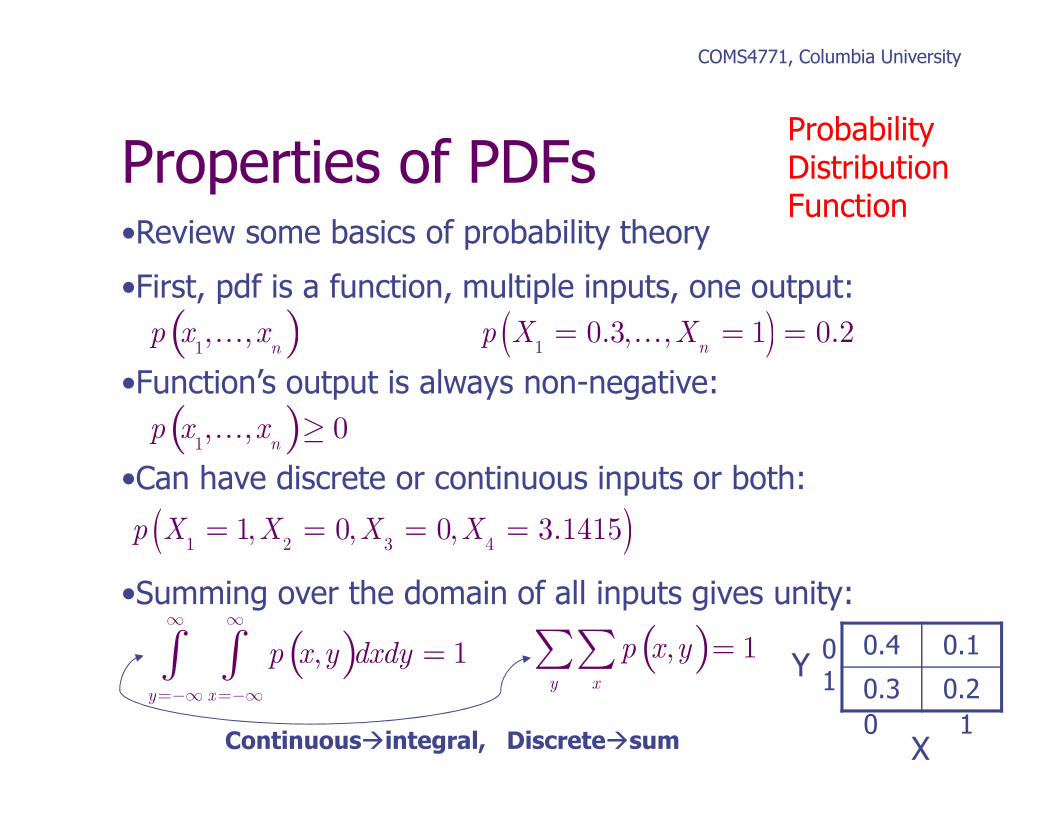
Properties of PDFs
COMS4771, Columbia University(Bishop PRML 1.2.1)
CDF Cumulative
Distribution
Function
D

COMS4771, Columbia University
Properties of PDFs•Marginalizing: integrate/sum out a variable leaves a
marginal distribution over the remaining ones…
•Conditioning: if a variable ‘y’ is ‘given’ we get aconditional distribution over the remaining ones…
•Bayes Rule: mathematically just redo conditioningbut has a deeper meaning (1764)… if wehave x being data and θ being a model
p x,y( )
y∑ = p x( )
p x | y( )=
p x,y( )p y( )
p θ | x( )=p x | θ( )p θ( )
p x( )posterior
likelihood
evidence
prior
COMS4771, Columbia University
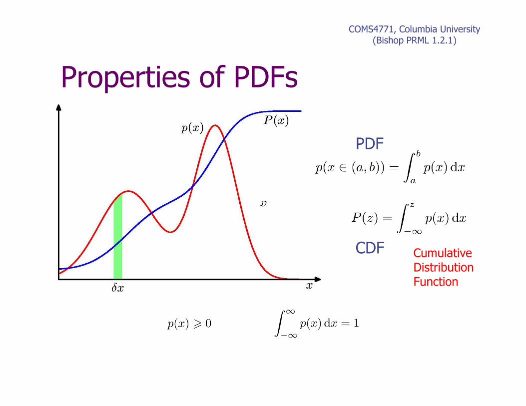
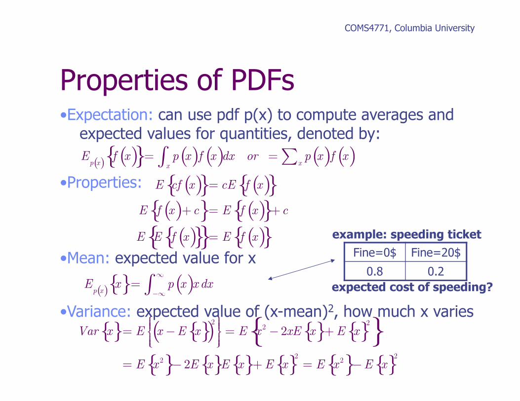
Properties of PDFs•Expectation: can use pdf p(x) to compute averages and
expected values for quantities, denoted by:
•Properties:
•Mean: expected value for x
•Variance: expected value of (x-mean)2, how much x varies E
p x( )x{}= p x( )x
−∞
∞
∫ dx
Fine=0$ Fine=20$
0.8 0.2
example: speeding ticket
expected cost of speeding?
E
p x( )f x( ){ }= p x( )f x( )
x∫ dx or = p x( )f x( )
x∑
Var x{}= E x −E x{}( )2
= E x
2− 2xE x{}+ E x{}
2{ }= E x
2{ }− 2E x{}E x{}+ E x{}2
= E x2{ }−E x{}
2
E cf x( ){ }= cE f x( ){ }E f x( )+c{ }= E f x( ){ }+c
E E f x( ){ }{ }= E f x( ){ }
COMS4771, Columbia University
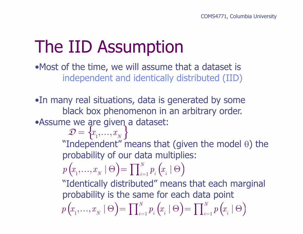
The IID Assumption•Most of the time, we will assume that a dataset is
independent and identically distributed (IID)
•In many real situations, data is generated by someblack box phenomenon in an arbitrary order.
•Assume we are given a dataset:
“Independent” means that (given the model θ) theprobability of our data multiplies:
“Identically distributed” means that each marginalprobability is the same for each data point
p x
1,…,x
N| Θ( )= p
ixi| Θ( )
i=1
N
∏
D = x
1,…,x
N{ }
p x
1,…,x
N| Θ( )= p
ixi| Θ( )
i=1
N
∏ = p xi| Θ( )
i=1
N
∏
Ex: Is a coin fair?
COMS4771, Columbia University
A stranger tells you his coin is fair.
Let’s assume tosses are iid with P(H)=µ.
He tosses it 4 times, gets H H T H.
What can you say about µ?
COMS4771, Columbia University
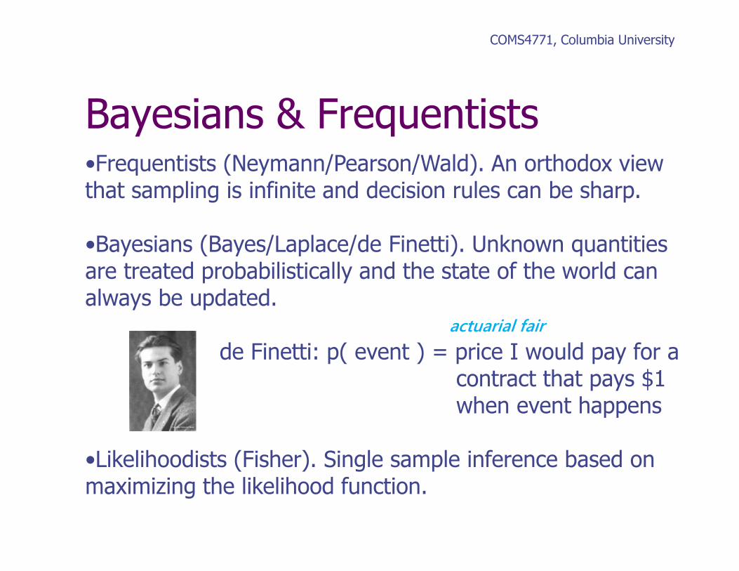
Bayesians & Frequentists•Frequentists (Neymann/Pearson/Wald). An orthodox view that sampling is infinite and decision rules can be sharp.
•Bayesians (Bayes/Laplace/de Finetti). Unknown quantities are treated probabilistically and the state of the world can always be updated.
de Finetti: p( event ) = price I would pay for acontract that pays $1when event happens
•Likelihoodists (Fisher). Single sample inference based on maximizing the likelihood function.
actuarial fair

COMS4771, Columbia University
Bayesians & Frequentists•Frequentists:
•Data are a repeatable random sample - there is a frequency •Underlying parameters remain constant during this repeatable process•Parameters are fixed
•Bayesians:•Data are observed from the realized sample.•Parameters are unknown and described probabilistically•Data are fixed

COMS4771, Columbia University
Frequentists
•Frequentists: classical / objective view / no priorsevery statistician should compute same p(x) so no priorscan’t have a p(event) if it never happenedavoid p(θ), there is 1 true model, not distribution of thempermitted: p
θ(x,y) forbidden: p(x,y|θ)
Frequentist inference: estimate one best model θuse the Maximum Likelihood Estimator (ML)(unbiased & minimum variance)do not depend on Bayes rule for learning
( )
( )1 2
|
Data
arg m x
, ,
a
,n
MLp
x x x
θθθ
=
=
…
D
D
COMS4771, Columbia University
Bayesians
•Bayesians: subjective view / priors are okput a distribution or pdf on all variables in the problemeven models & deterministic quantities (speed of light)use a prior p(θ) on the model θ before seeing any data
Bayesian inference: use Bayes rule for learning, integrateover all model (θ) unknown variables

COMS4771, Columbia University
Bayesian Inference•Bayes rule can lead us to maximum likelihood•Assume we have a prior over models p(θ)
•How to pick p(θ)?Pick simpler θ is betterPick form for mathematical convenience
•We have data (can assume IID):
•Want to get a model to compute:
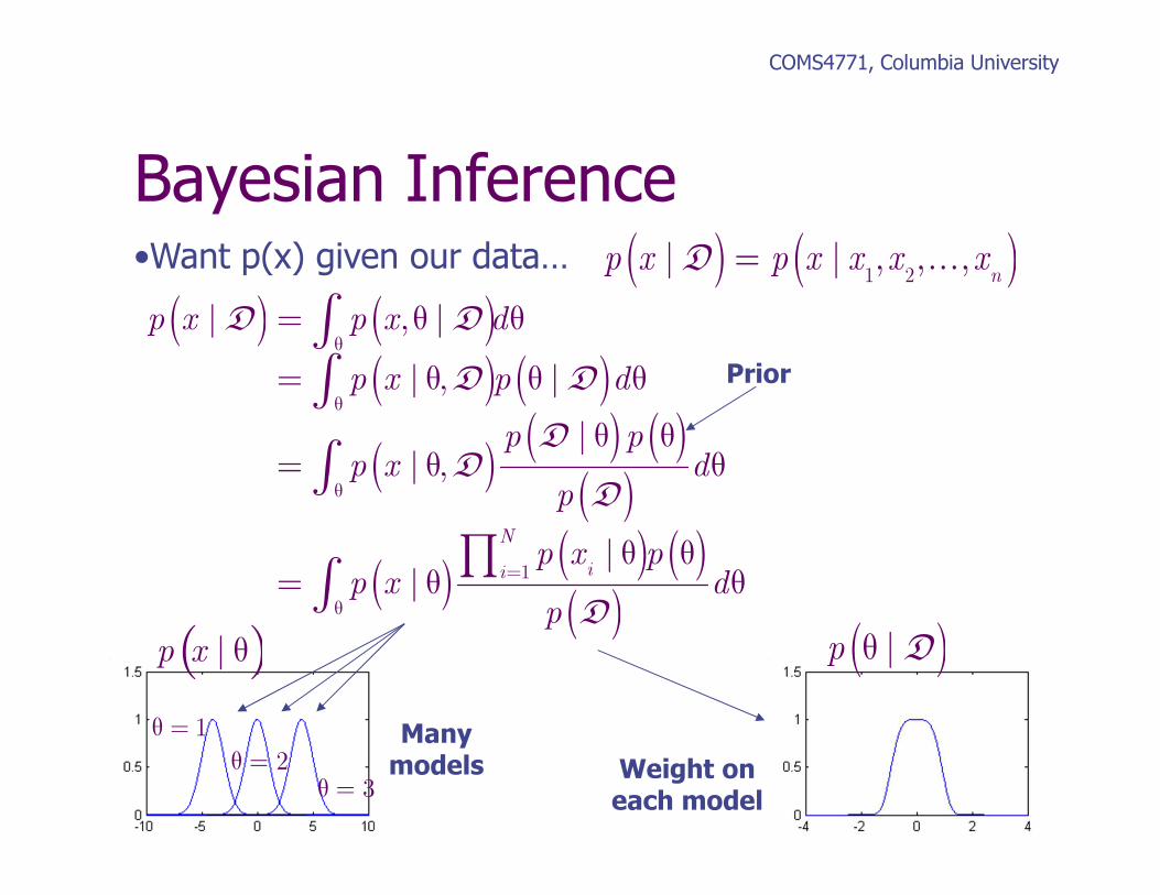
•Want p(x) given our data… How to proceed?
( )( ) ( )
( )
||
p x p
p x
p x
θ θθ =
posterior
likelihood
evidence
prior
{ }D1 2, , ,
Nx x x= …
( )p x
( )p θ
COMS4771, Columbia University
Bayesian Inference•Want p(x) given our data… ( ) ( )D
1 2| | , , ,
n
p x p x x x x= …
( ) ( )( ) ( )
( )( ) ( )
( )
( )( ) ( )( )
D D
D D
DD
D
D
1
| , |
| , |
|| ,
||
N
ii
p x p x d
p x p d
p pp x d
p
p x pp x d
p
θ
θ
θ
=
θ
= θ θ
= θ θ θ
θ θ= θ θ
θ θ= θ θ
∫∫
∫
∏∫
p x | θ( ) ( )D|p θ
Manymodels Weight on
each model
θ = 1
θ = 2
θ = 3
Prior
COMS4771, Columbia University
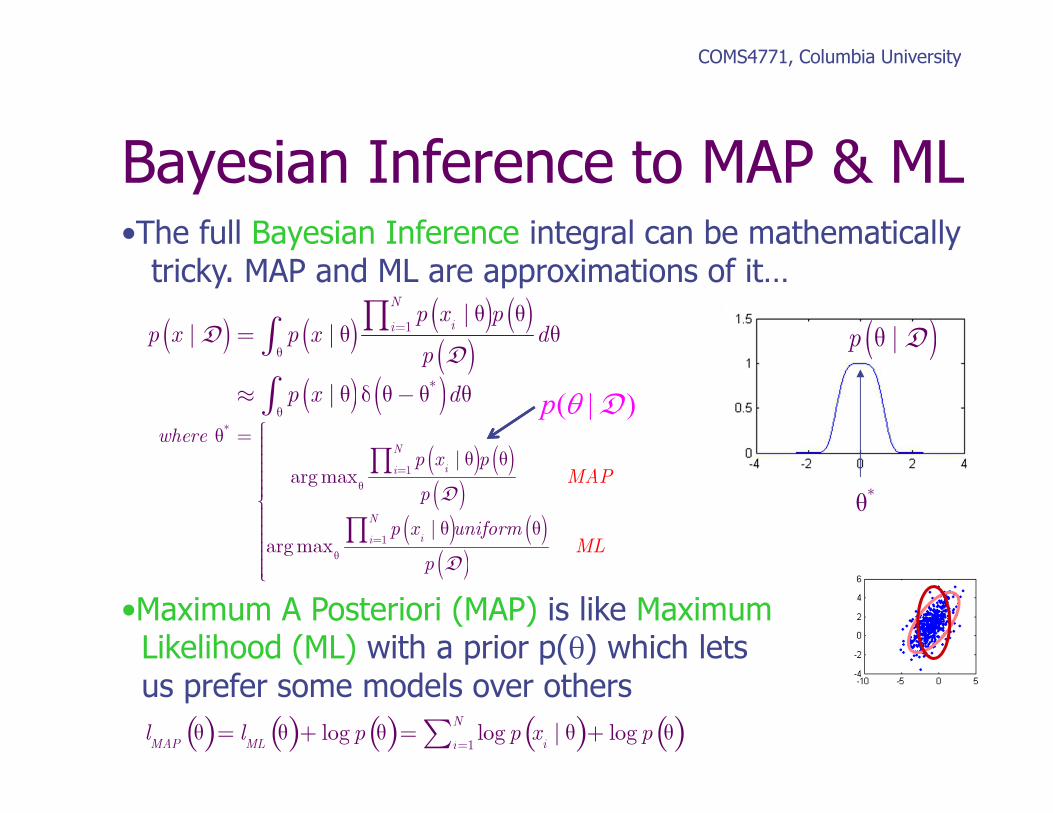
Bayesian Inference to MAP & ML•The full Bayesian Inference integral can be mathematicallytricky. MAP and ML are approximations of it…
•Maximum A Posteriori (MAP) is like MaximumLikelihood (ML) with a prior p(θ) which letsus prefer some models over others
( ) ( )( ) ( )( )
( ) ( )
DD
1
*
|| |
|
N
iip x p
p x p x dp
p x d
=
θ
θ
θ θ= θ θ
≈ θ δ θ − θ θ
∏∫
∫
( ) ( )( )
( ) ( )( )
D
D
*
1
1
|argmax
|argmax
N
ii
N
ii
where
p x p
p
p x
MAP
MLuniform
p
=
θ
=
θ
θ =
θ θ θ θ
∏
∏
( )D|p θ
θ*
lMAP
θ( )= lML
θ( )+ log p θ( )= log p xi| θ( )
i=1
N
∑ + log p θ( )
( | )p θ D

Ex: Is a coin fair?
COMS4771, Columbia University
A stranger tells you his coin is fair.
Let’s assume tosses are iid with P(H)=µ.
He tosses it 4 times, gets H H T H.
What can you say about µ?
( ), , ,H H T H=D
COMS4771, Columbia University
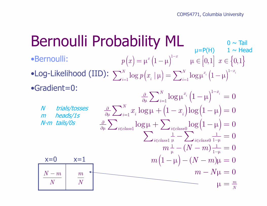
Bernoulli Probability ML•Bernoulli:
•Log-Likelihood (IID):
•Gradient=0:
( ) ( ) { }1
1 0,1 0,1x
x
p x x−
= − ∈ ∈ µ
µ µ
( ) ( )1
1 1log | log 1
ii
xN N x
ii ip x
−
= =
= −µ µ µ∑ ∑
( )( ) ( )
( )
( )
1
1
1
1 0
1 1
11 0
1 1
1
log 1 0
log 1 log 1 0
log log 1 0
0
( ) 0
1 ( ) 0
0
ii
xN x
i
N
i ii
i class i class
i class i class
m
N
x x
m N m
m N m
m N
−∂
∂ =
∂
∂ =
∂
∂ ∈ ∈
µ
µ
µ
µ µ
µ
−∈ ∈
µ−
− =
+ − − =
+ − =
− =
− − =
− − − =
µ µ
µ µ
µ µ
µ µ
µ
− =
=
µ
∑
∑
∑ ∑∑ ∑
x=0 x=1
m
N
N m
N
−
0 ~ Tail1 ~ Headµ=P(H)
N trials/tossesm heads/1sN-m tails/0s
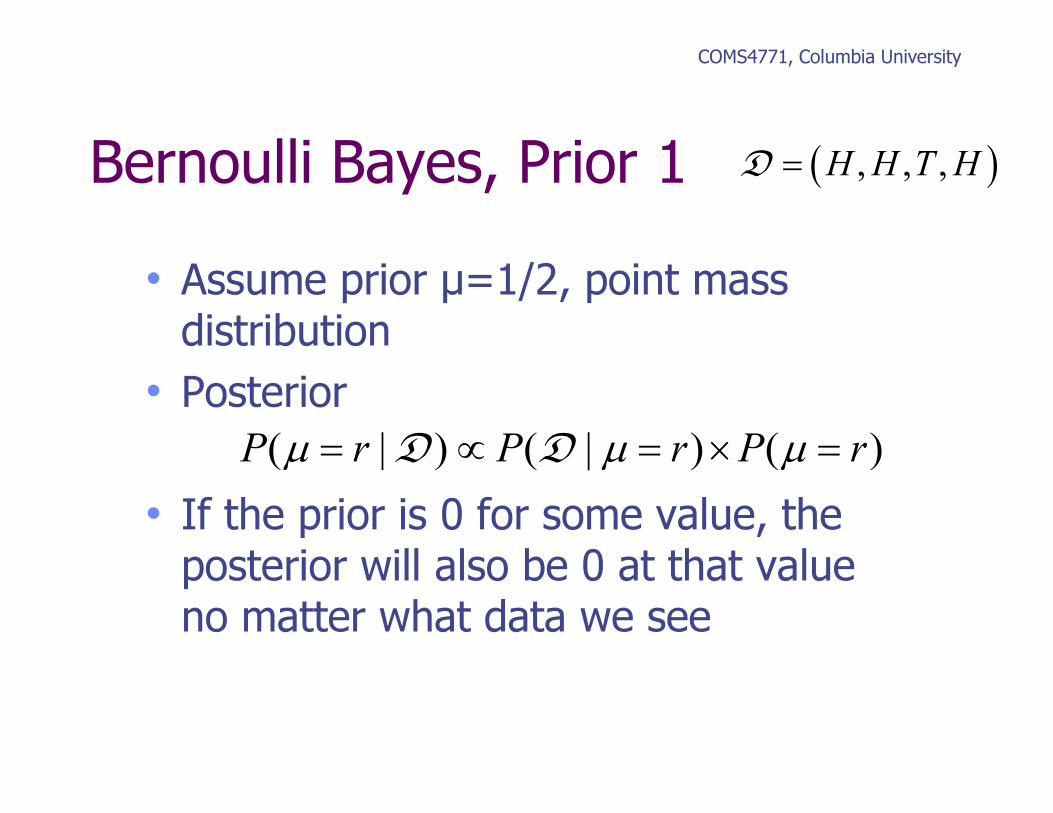
Bernoulli Bayes, Prior 1
• Assume prior µ=1/2, point mass distribution
• Posterior
• If the prior is 0 for some value, the posterior will also be 0 at that value no matter what data we see
COMS4771, Columbia University
( ), , ,H H T H=D
( ) ( || ) ( )P Pr r P rµ µ µ= = ×∝ =D D

Bernoulli Bayes, Prior 2
• Allow some chance of bias
• Prior P(µ=1/2) = 1-b
P(µ=3/4) = b
• Posterior
COMS4771, Columbia University
( ), , ,H H T H=D
4
3
( ) ( |
3 1( ) ( |
4
1 1 1 1| ) ( ) (1 )
2 2 2 2
3 3 3| ) ( )
4 4 44
P
bP
P bP
P P
µ µ µ
µ µ µ
= = × = = × −
= = × =
∝
∝ = ×
D D
D D
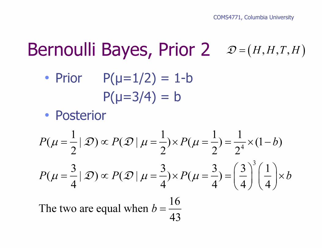
Bernoulli Bayes, Prior 2
• Prior P(µ=1/2) = 1-b
P(µ=3/4) = b
• Posterior
COMS4771, Columbia University
( ), , ,H H T H=D
4
3
1 1 1 1| ) ( ) (1 )
2 2 2 2
3 3 3| ) ( )
4 4 4
The two are equal
( ) ( |
3 1
when
( ) ( |4 4
16
43
P b
P b
b
P P
P P
µ µ µ
µ µ µ
= = × = = × −
= = × = = ×
∝
∝
=
D D
D D

Bernoulli Bayes, Prior 3
• Uniform prior
COMS4771, Columbia University
( ), , ,H H T H=D
3
13
0
3
| ) ( )
) (1 )
1 1 1(1 )
4 5 20
Hence posterior | (1 )
Notice for tosses with m
( ) ( |
( |
( ) 20
, tails,
( |
Does this sugg
heads
est a convenient
) (1 )
prior?
m N m
P P
P
P r
N m
r r P r
r r r
r r dr
r r rP
r r
N
µ µ µ
µ
µ
µ−
= = × =
=
∝
= −
− = − =
= −
= = −
=
−
∫
D D
D
D
D
[0,1]Uµ ∼
Where’s the mode?
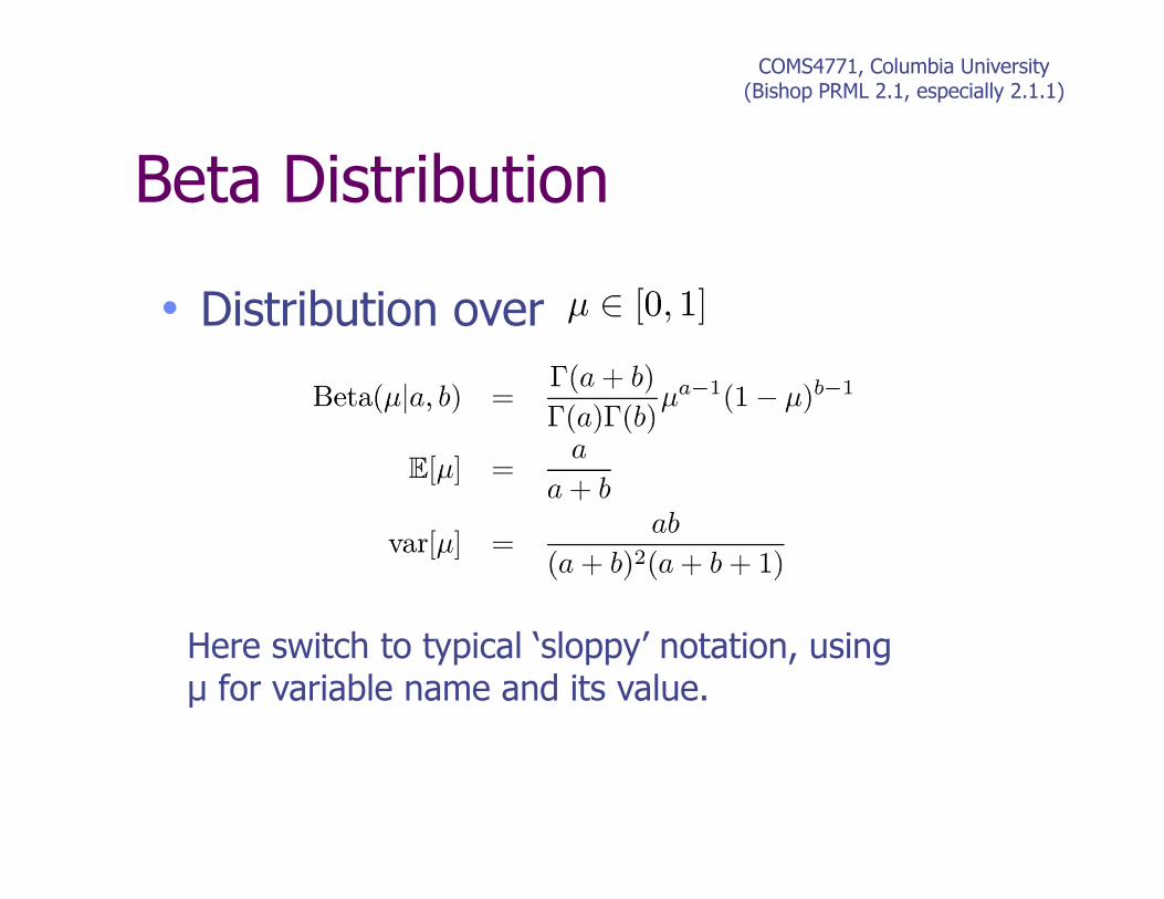
Beta Distribution
• Distribution over
COMS4771, Columbia University(Bishop PRML 2.1, especially 2.1.1)
Here switch to typical ‘sloppy’ notation, using µ for variable name and its value.

Bernoulli Bayes, Beta Prior
The Beta distribution provides the conjugate prior for the Bernoulli distribution, i.e. the posterior distribution has the same form as the prior.
effective number of observations +1
All distributions in the Exponential Family (includes multinomial, Gaussian, Poisson) have convenient conjugate priors (Bishop PRML 2.4).
COMS4771, Columbia University(Bishop PRML 2.1, especially 2.1.1)

Beta Distribution
COMS4771, Columbia University(Bishop PRML 2.1, especially 2.1.1)
Which distribution is this?

Prior · Likelihood = Posteriornormalized
COMS4771, Columbia University(Bishop PRML 2.1, especially 2.1.1)
Example:
a=2, b=2 a=3, b=2Single observationH or x=1
Recall our earlier example of a Uniform prior, check this works…
)(p µ ( | )p µD |( )p µ D

Properties of the Posterior
As the size of the data set, N, grows
COMS4771, Columbia University(Bishop PRML 2.1, especially 2.1.1)
0
0 0
2var[
[ ]
] 0( ) ( 1)
N
ML
N N
N N
N N N N
a a m m
a b a m b N m N
a b
a b a b
µ µ
µ
+= = → =
+ + + + −
= →
+ + +
E
This is typical behavior for Bayesian learning.

Prediction under the PosteriorWhat is the probability that the next coin toss will land heads up?
COMS4771, Columbia University(Bishop PRML 2.1, especially 2.1.1)
N
N N
a
a b+
( ) 1 1 1, ,, 3,N N
H H a bT H= ⇒ = + = +D

Bayesian Decision Theory
• Initially assume just 2 classes
• Given input data we want to determine which class is optimal
• Various possible criteria
• Need either directly (discriminative)
• Or by Bayes,
(generative)
• Divide input space into decision regions separated by decision boundaries such that
• How might we choose boundaries?
COMS4771, Columbia University(Bishop PRML 1.5)
1 2, C C
x
|( )k
p xC
( , ( || )
( )
) ) ( )
( )( k k k
k
p x p xx
p x
pp
p x= =
C C CC
1 2,R R
assign k k
x∈ ⇒R C
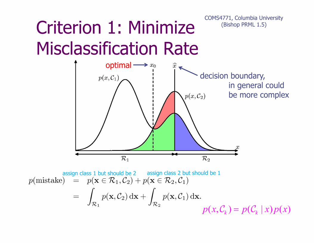
Criterion 1: Minimize Misclassification Rate
COMS4771, Columbia University(Bishop PRML 1.5)
decision boundary,in general couldbe more complex
optimal
( , ) ( | ) ( )k k
p x p x p x=C C
assign class 1 but should be 2 assign class 2 but should be 1

Criterion 2: Minimize Expected LossExample loss matrix:
classify medical images as ‘cancer’ or ‘normal’
DecisionTruth
COMS4771, Columbia University(Bishop PRML 1.5)
Now
Choose regions to minimize Expected LossjR
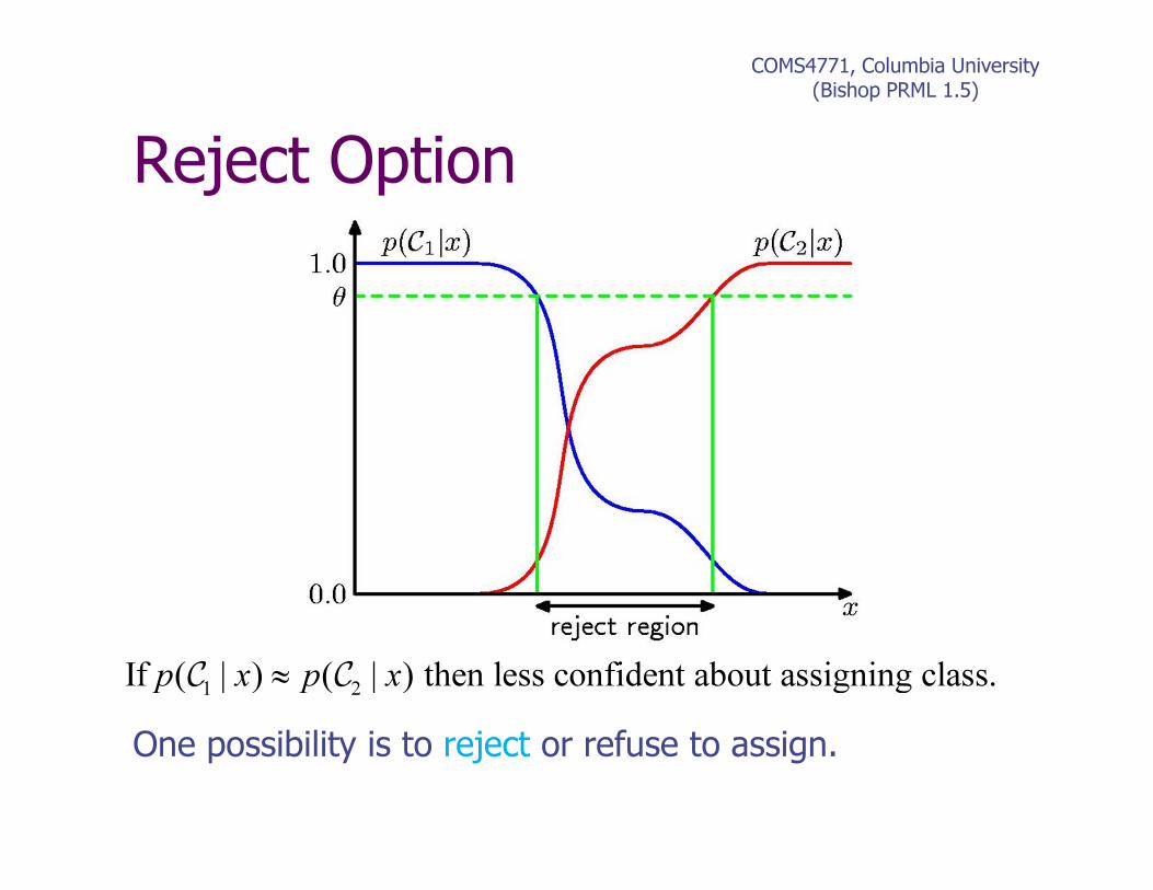
Reject Option
COMS4771, Columbia University(Bishop PRML 1.5)
1 2| ) ( | ) then less confident about assigning claI s( s.f x p xp ≈C C
One possibility is to reject or refuse to assign.
Related Documents