MA 112/227 PROBABILITY LECTURE NOTES - …cathal/Teaching/Lecture_notes...MA 112/227 PROBABILITY LECTURE NOTES Cathal Seoighe Room C204 (Aras De Brun´ ), [email protected]´

MA 112/227 PROBABILITYLECTURE NOTES

Cathal Seoighe Room C204 (Aras De Brun), [email protected]

GENERAL INFORMATION

SYLLABUS

The role of probability theory in modelling random phenomena and instatistical decision making

sample spaces and events

some basic probability formulae

conditional probability and independence

Bayes’ formula

counting techniques

discrete and continuous random variables

hypergeometric and binomial distributions

Poisson distributions

normal distributions

the distribution of the sample mean when sampling from a normal distri-bution

the Central Limit Theorem with applications including normal approxi-mations to binomial distributions.

SAMPLE TEXTS (most of these texts include statistics as well aschapters on probability that are relevant to this course)

Wackerly, Mendenhall, and Scheaffer Mathematical statistics with applica-tions, 6th Ed. Main Library 519.5 MEN

Freund, John E. Modern Elementary Statistics 519.5 FRE

Wonnacott, Thomas H. Introductory Statistics Main Library 519.5 WON

Lipschutz, Seymour Schaum’s outline of theory and problems of introduc-tion to probability and statistics. Main Library 519.2 LIP

1

Freund, John E. John E. Freund’s mathematical statistics : with applica-tions. 2004 (and other versions) Main Library 519.5 FRE (also versionswith authors Miller, Irwin]

Pestman, Wiebe R., Mathematical statistics : an introduction 1998 MainLibrary 519.5 PES Mendenhall, William Mathematical statistics with ap-plications 1990 Main Library 519.5 MEN

SAMPLE ELECTRONIC RESOURCES:

Click on some of the On-Line texts athttp://people.hofstra.edu/liora p schmelkin/weblink/methods.html

A textbook is available online athttp://www.dartmouth.edu/∼chance/teaching aids/books articles/probabilitybook/amsbook.mac.pdf. This is a relatively advanced textbook but it doescover the material in this course.

Lectures: Tuesdays at 11:10 am in AC 201 and Thursdays at 11:10 am inAC202.

Tutorials: TBA. Commencement date will be announced in class.

Assessment: Assessment will consist of homework, class test, and a final exam.Please attend all lectures

2

These notes contain a synopsis of the theory that will be covered in this course,followed by worked example questions.

Why study probability?

In the real world we often want to predict what will happen (e.g. what is thechance of 6 numbers right in the next draw of the Lotto; many applications inscience, communications, finance, gambling, weather forecasting, and just aboutall fields of human endeavour). Probability is also the basis of all of statistics.It crops up pretty much everywhere from biology to games to psychology.

What is Probability?

There is still some debate about how to think about probability and the issuescan become quite philosophical (what is it? how should we interpret it? is itsubjective? etc.) Mathematically, the picture is clearer. Probabilities have tosatisfy certain properties - e.g. a probabilty can never be a negative number.These properties are provided later, together with a brief overview of some ofthe different interpretations of probability.

Some definitions

Experiment: In probability, an experiment is anything that gives rise to adefined set of possible outcomes. E.g. toss a con once, roll a die twice, pick aperson at random from the cancer unit of a hospital, measure the temperaturetomorrow, count the number of cars that arrive on Campus between 9am and9:01 am on a random day). By definition, an experiment is the process by whichwe obtain data, and is intended to include scientific experiments and observa-tional studies; note that an experiment implies more control over extraneousvariables than happens in a observational study.

Sample space: The sample space, Ω (or S), is the set of all possible outcomesof the experiment.

For example, if the ‘experiment’ is a single die toss the sample space is 1,2,3,4,5,6

Event: A subset A of Ω is called an event. A singleton subset is referred toas an elementary event or basic outcome or sample point. An event is said tooccur if the outcome of the experiment is a member of the set A.

For example, an even number coming up in a single die toss is an event. In thiscase A = 2,4,6. An event can contain a single sample point, e.g. A = 1 isthe event that a one comes up in a single die toss.

Probability: A probability function assigns a number (its probability) to eachevent A (i.e. it is a mapping from events to numbers on the real line). There

3

are some technical issues that have to do with what kinds of subsets can haveprobabilitites assigned to them, but these are beyond the scope of this course.

Back to the definition of probability

Classical or “equally likely” definition of probability If Ω has a finitenumber of equally likely elements, then we compute P (A) from the formulaP (A) = # elements in A

# elements in Ω .

Empirical or statistical or relative frequency definition of probabilityP (A) is defined as the limit, as N −→ ∞, of the proportion of times A willoccur in N repetitions of the experiment.

Logical or Bayesian or subjective definition of probability : Probabilityindicates the degree of plausibility of a proposition, given the available evidence.Emphasizes the conditional nature of probability (always depends on what youknow). Seen as an extension of Aristotolean logic to accommodate uncertainty.

Axiomatic definition of probability: As seen above, we can think of aprobability as a mathematical function that maps the subsets of Ω to the realnumbers. In order for this function to be called a probability function it has tosatisfy certain criteria (given next).

Probability axioms (Kolmogorov)

A probability function on subsets of Ω must satisfy these conditions

1. P (Ω) = 1, where Ω is the sample space.

2. P (A) ≥ 0 for all A.

3. P (∪∞i=1Ai) =∑∞

i=1 P (Ai) if Ai, i = 1, 2, ...,∞ are pairwise disjoint, i.e.mutually exclusive (i.e. Ai ∩Aj = ∅).

Tools for solving probability problems

Most basic problems in probability can be solved using a combination of therules of probability and combinatorics (i.e. counting). These rules are listedbelow. In class we will derive most of the probability formulae from the axiomsabove.

4

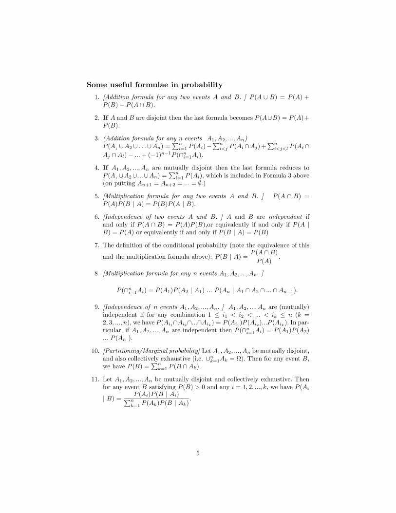
Some useful formulae in probability

1. [Addition formula for any two events A and B. ] P (A ∪ B) = P (A) +P (B)− P (A ∩B).

2. If A and B are disjoint then the last formula becomes P (A∪B) = P (A)+P (B).

3. (Addition formula for any n events A1, A2, ..., An)P (A1 ∪A2 ∪ . . .∪An) =

∑ni=1 P (Ai)−

∑ni<j P (Ai ∩Aj)+

∑ni<j<l P (Ai ∩

Aj ∩Al)− ... + (−1)n−1P (∩ni=1Ai).

4. If A1, A2, ..., An are mutually disjoint then the last formula reduces toP (A1 ∪A2∪ ...∪An) =

∑ni=1 P (Ai), which is included in Formula 3 above

(on putting An+1 = An+2 = ... = ∅.)

5. [Multiplication formula for any two events A and B. ] P (A ∩ B) =P (A)P (B | A) = P (B)P (A | B).

6. [Independence of two events A and B. ] A and B are independent ifand only if P (A ∩ B) = P (A)P (B),or equivalently if and only if P (A |B) = P (A) or equivalently if and only if P (B | A) = P (B)

7. The definition of the conditional probability (note the equivalence of this

and the multiplication formula above): P (B | A) =P (A ∩B)

P (A).

8. [Multiplication formula for any n events A1, A2, ..., An. ]

P (∩ni=1Ai) = P (A1)P (A2 | A1) ... P (An | A1 ∩A2 ∩ ... ∩An−1).

9. [Independence of n events A1, A2, ..., An. ] A1, A2, ..., An are (mutually)independent if for any combination 1 ≤ i1 < i2 < ... < ik ≤ n (k =2, 3, ..., n), we have P (Ai1∩Ai2∩...∩Aik

) = P (Ai1)P (Ai2)...P (Aik). In par-

ticular, if A1, A2, ..., An are independent then P (∩ni=1Ai) = P (A1)P (A2)

... P (An ).

10. [Partitioning/Marginal probability] Let A1, A2, ..., An be mutually disjoint,and also collectively exhaustive (i.e. ∪n

k=1Ak = Ω). Then for any event B,we have P (B) =

∑nk=1 P (B ∩Ak).

11. Let A1, A2, ..., An be mutually disjoint and collectively exhaustive. Thenfor any event B satisfying P (B) > 0 and any i = 1, 2, ..., k, we have P (Ai

| B) =P (Ai)P (B | Ai)∑n

k=1 P (Ak)P (B | Ak).

5

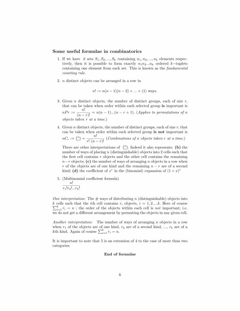
Some useful formulae in combinatorics

1. If we have k sets S1, S2, ..., Sk containing n1, n2, ..., nk elements respec-tively, then it is possible to form exactly n1n2...nk ordered k−tupletscontaining one element from each set. This is known as the fundamentalcounting rule.

2. n distinct objects can be arranged in a row in

n! := n(n− 1)(n− 2)× ...× (1) ways.

3. Given n distinct objects, the number of distinct groups, each of size r,that can be taken when order within each selected group is important is

nPr :=n!

(n− r)!= n(n − 1)...(n − r + 1). (Applies to permutations of n

objects taken r at a time.)

4. Given n distinct objects, the number of distinct groups, each of size r, thatcan be taken when order within each selected group is not important is

nCr :=(nr

)=

n!r! (n− r)!

(Combinations of n objects taken r at a time.)

There are other interpretations of(nr

). Indeed it also represents: (b) the

number of ways of placing n (distinguishable) objects into 2 cells such thatthe first cell contains r objects and the other cell contains the remainingn−r objects; (c) the number of ways of arranging n objects in a row whenr of the objects are of one kind and the remaining n − r are of a secondkind; (d) the coefficient of xr in the (binomial) expansion of (1 + x)r

5. (Multinomial coefficient formula)n!

r1!r2!...rk!

One interpretation: The # ways of distributing n (distinguishable) objects intok cells such that the ith cell contains ri objects, i = 1, 2, ...k. Here of course∑k

i=1 ri = n ; the order of the objects within each cell is not important; i.e.we do not get a different arrangement by permuting the objects in any given cell.

Another interpretation: The number of ways of arranging n objects in a rowwhen r1 of the objects are of one kind, r2 are of a second kind, ..., rk are of akth kind. Again of course

∑ki=1 ri = n.

It is important to note that 5 is an extension of 4 to the case of more than twocategories.

End of formulae

6

Discrete random variables

Often what we are interested in is some number which is associated with theoutcome of the experiment rather than in the detailed outcome of the experi-ment. For example, when we flip a coin a number of times, we might not be somuch interested in the sides that come up, but rather in the number of timeseach side arises. Similarly, when a person is picked at random, we may well notbe interested in the person’s name, but rather some number associated withhim/her, such as height or weight or income. The fact that so often the out-comes in probability experiments are mapped to numbers leads to the conceptof the random variable

A random variable X is a function that associates a number with each ele-ment of the sample space S of an experiment. An easier way to think about athis is that a random variable X represents a numerical quantity, the value ofwhich depends on the outcome of the experiment.

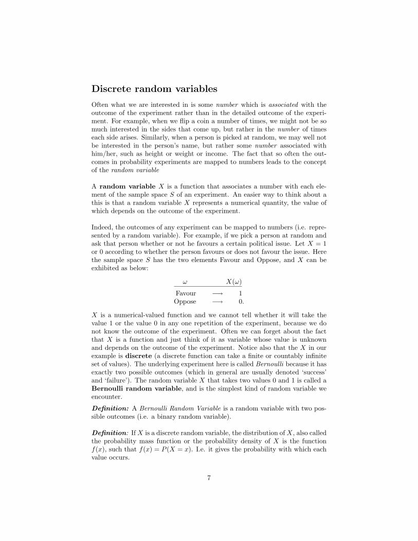
Indeed, the outcomes of any experiment can be mapped to numbers (i.e. repre-sented by a random variable). For example, if we pick a person at random andask that person whether or not he favours a certain political issue. Let X = 1or 0 according to whether the person favours or does not favour the issue. Herethe sample space S has the two elements Favour and Oppose, and X can beexhibited as below:

ω X(ω)

Favour −→ 1Oppose −→ 0.

X is a numerical-valued function and we cannot tell whether it will take thevalue 1 or the value 0 in any one repetition of the experiment, because we donot know the outcome of the experiment. Often we can forget about the factthat X is a function and just think of it as variable whose value is unknownand depends on the outcome of the experiment. Notice also that the X in ourexample is discrete (a discrete function can take a finite or countably infiniteset of values). The underlying experiment here is called Bernoulli because it hasexactly two possible outcomes (which in general are usually denoted ‘success’and ‘failure’). The random variable X that takes two values 0 and 1 is called aBernoulli random variable, and is the simplest kind of random variable weencounter.

Definition: A Bernoulli Random Variable is a random variable with two pos-sible outcomes (i.e. a binary random variable).

Definition: If X is a discrete random variable, the distribution of X, also calledthe probability mass function or the probability density of X is the functionf(x), such that f(x) = P (X = x). I.e. it gives the probability with which eachvalue occurs.

7

Note that in any discrete distribution, the probabilities are non-negative andmust add to one; this is another definition of a distribution.

Mean and Variance

The mean and variance are often used to summarize a distribution.

Definition: Let X be a discrete random variable. The mean value of X orexpected value of X,or population mean (sometimes loosely called the averagevalue of X) is the centre of gravity of the distribution of X and is defined as

µ := E(X) =∑

x

xP (X = x)

(that is, multiply each value x of X by its probability P (X = x) and add).

The E here stands for Expected. Another word for the mean of the distributionis the expected value.

Definition: The variance of X, also called the population variance, is definedby:

V ar(X) =∑

x

(x− µ)2P (X = x)

Finally, the standard deviation of X, which is traditionally given the symbolσ, is simply σ =

√V ar(X). The standard deviation rather than the variance

of a distribution is often quoted and for this reason the variance is sometimesreferred to as σ2.

Interpretation of µ and σE(X) (the mean of the distribution) is the ‘long-term average’ value of the ran-dom variable. For example, suppose you are involved in a work sweepstake.Each week you get ¿20 if you win and have a probability of 0.04 of winningand probability 0.96 of not winning. After a large number of weeks you wouldexpect to have won about 4% of the time. The formula for E(X) is logical: ifyou play the game many many times, you will win about 4% of the time andget ¿20 and lose about 96% of the time and get ¿0. If this went on for 1000weeks you would expect to come away with about 1000 × (0.04× ¿20 +0.96׿0 = 1000× 0.8

Your long-term average (i.e. E(X)) winnings would be 1000×0.81000 = 0.8

In a real sense it is worth about 80 cents to you per week to play this sweepstake.Of course if you are paying ¿1 per week to play you can expect to make a net

8

loss in the long term.

Somewhat similarly, σ2 tells you how large, on average, (x−µ)2 is (the formulafor the variance just multiplies each value of (x − µ)2 by how likely that valueis to occur and adds them all up). This tells you something about how far, onaverage, you are from the mean of the distribution.

For example, consider two students who take a course with continuous assess-ment. One student is eratic and only hands in some of the assignments, butthe assignmetns completed are done well. The other student completes all theassignment but does a mediocre job each time. Suppose both students get agrade of 50% for the course. The marks of the first student would be expectedto show a higher variance from the mean, reflecting his eratic behaviour.

Two important discrete distributions

The binomial and hypergeometric distributions both occur in problems in-volving the number of successes or failures in n Bernoulli trials (recall that aBernoulli trial is an experiment that can have one of two possible outcomes).

Binomial distribution

Consider a random variable, X, which represents the number of successes wewill obtain in n independent Bernoulli trials. If p denotes the probability of asuccess on any one trial then

P (X = x) =(nx

)px(1− p)n−x, x = 0, 1, 2, ..., n. .

Formal definition: A random variable X has a binomial distribution withparameters n and p [abbreviated X ∼ Bin(n, p)] if its mass function, f(x) is

f(x) := P (X = x) =(nx

)px(1− p)n−x, x = 0, 1, 2, ..., n. .

[Some texts use π or θ for p. Note also that many texts denote 1 − p by theletter q, denoting the probability of failure on any one trial.]

Mean and variance of the binomial distribution

If X is a binomially distributed random variable, then the mean and varianceof X are

E(X) := µX := µ = np, and V ar(X) := σ2X := σ2 = np(1− p).

9

Hypergeometric distribution

Consider now the number of successes we obtain when n items are taken withoutreplacement from a population that consists of N items, of which a are of onekind (successes) and the remaining N −a are of a second kind (failures). Unlikein the case of the binomial random variable the number of successes you haveobtained so far influences whether the next trial is a success or not, becausethe number of successes in the population is reduced by one every time yousample a success. I.e. p, the probability of sampling a success, changes in thehypergeometric case but remains fixed for the binomial

Formal definition: A random variable X has a hypergeometric distributionif its mass function is

f(x) := P (X = x) =

(ax

)(N−an−x

)(Nn

) , x = 0, 1, 2, ...,min(a, n).

Mean and variance of the hypergeometric distribution

If X is a hypergeometric random variable, then the mean and variance of X are

E(X) := µX := µ = n aN , and V ar(X) := σ2

X := σ2 = n aN (1− a

N )N−nN−1 .

How do I know if I should use the binomial or hypergeometric?Consider an experiment that consists of n identical trials, where each trial isBernoulli (i.e. has only two possible outcomes, ‘success’ and ‘failure’), e.g. pickn people at random from a room and observe if the person is male or female,pick n companies at random and observe if each individual company made aprofit or loss last year. To find the distribution of X, the number of successes inthe n trials, use the hypergeometric below if the trials involve sampling withoutreplacement from a finite population and use the binomial formula below if thetrials are independent and the probability of a success is the same from trial totrial (as in choosing people with replacement from a room, or tossing a coin ntimes).

Note: In situations where the hypergeometric is appropriate, you can approxi-mate it using the (easier) binomial if n/N ≤ 0.05.

The Poisson process

The Poisson process arises when we want to model the number of arrivals inan interval of time or space. Here we use the word arrivals in a broad sense tomean occurrences of something in space or events in time).

10

Examples of processes that produce arrivals are:

the observation of disintegration of atoms of a radioactive substance,

the occurrence of goals in a football game, the occurrence of defects in asheet of carpet,

the occurrence of phone calls to a telephone exchange throughout the day,

the occurrence of typographical errors in a manuscript, etc.

In each of the above, the following three assumptions seem reasonable

1. In a small time interval or amount of space, the probability of occurrenceof the event of interest is proportional to the size of the interval (e.g., it istwice as likely to find a defect in the next two metres of carpet as in thenext metre, it is five times as likely that a goal will be scored in the nextfive minutes of a soccer game as in the next minute);

2. The probability of two or more occurrences in small time or space intervalis negligible compared with the probability of one occurrence (e.g. thechance of two or more goals in the next minute of a soccer game is muchless likely than the probability of one goal, the chance of two or morepeople arriving at the bank in the next second is very small comparedwith the probability of one person arriving, etc.);

3. Arrivals in non-overlapping intervals are independent (e.g. the number ofarrivals at the bank between 10 and 10:01 am should not affect the numberof arrivals between 11:00 and 11:01 am).

Using these assumptions it is possible to show that X := the number of ar-rivals/occurrences in any time period of length t (or region of size t) has adistribution of the following form, for some positive number α :

f(x) = P (X = x) = e−αt (αt)x

x!, x = 0, 1, 2, ...,∞ (*)

(Question: Why is (*) a probability mass function?)The number α represents the arrival rate, i.e. the mean number of arrivals perunit time. It can be shown that E(X) = αt and that in fact V ar(X) is also αt.

Poisson approximation to the Binomial

Suppose that the Binomial distribution with parameters n and p is appropriatemodel for a random variable X. If n ≥ 20 and p ≤ 0.05, it can be shown thatthe Poisson distribution (with αt = np) can be used instead, as a good approx-imation, to work out probabilities about X. The approximation is excellent ifn ≥ 100 and np ≤ 10.

11

Continuous random variables

A random variable is called continuous if it can take values anywhere in aninterval. For a continuous random variable X, we shall consider a curve, calledthe density function f(x) of X such that the area under this curve between anytwo points a and b gives the probability that X lies between a and b. (Such afunction f(x) will be non-negative for every real number x, and the total areaunder it will be one.)

Definition: The probability density function, f(x), of a random variable, X,is the function such that

∫ b

af(x) = P (a ≤ X ≤ b)

An alternative way to describe a continuous random variable is through thecumulative distribution function. The cumulative distribution function, F (x),gives the probability that the random variable takes on a value less than orequal to x.

Definition: The cumulative distribution function, F , of a random variable isthe function such that F (x) = P (X ≤ x)

If X is a continuous random variable, the definitions of the population meanµ = E(X), the population variance σ2 = V ar(X), and the population standarddeviation σ =

√V ar(X) require calculus but the interpretation is relatively

straightforward. If we took a large sample of a the random variable and calcu-lated the mean and variance of the sample (called the sample mean and samplevariance, respectively), then the mean and variance of the continuous randomvariable would be approximated by the sample mean and sample variance. Ofcourse, this also holds true for discrete random variables.

An important continuous random variable: The normal dis-tribution

Continuous random variables that have a normal distribution are the most fre-quently encountered, as a consequence of the Central Limit Theorem (see next).The height of a random person, the sales of a company on a random day, themark of a random student on an exam, etc., are all often modelled by a normaldistribution. The density function of a normal random variable X that hasmean µ and variance σ2 is given by

f(x) =1√2πσ

exp−12σ2

(x− µ)2

,−∞ < x < ∞.

12

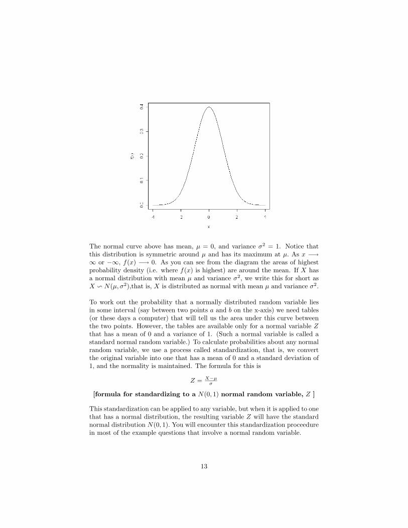
The normal curve above has mean, µ = 0, and variance σ2 = 1. Notice thatthis distribution is symmetric around µ and has its maximum at µ. As x −→∞ or −∞, f(x) −→ 0. As you can see from the diagram the areas of highestprobability density (i.e. where f(x) is highest) are around the mean. If X hasa normal distribution with mean µ and variance σ2, we write this for short asX v N(µ, σ2),that is, X is distributed as normal with mean µ and variance σ2.

To work out the probability that a normally distributed random variable liesin some interval (say between two points a and b on the x-axis) we need tables(or these days a computer) that will tell us the area under this curve betweenthe two points. However, the tables are available only for a normal variable Zthat has a mean of 0 and a variance of 1. (Such a normal variable is called astandard normal random variable.) To calculate probabilities about any normalrandom variable, we use a process called standardization, that is, we convertthe original variable into one that has a mean of 0 and a standard deviation of1, and the normality is maintained. The formula for this is

Z = X−µσ

[formula for standardizing to a N(0, 1) normal random variable, Z ]

This standardization can be applied to any variable, but when it is applied to onethat has a normal distribution, the resulting variable Z will have the standardnormal distribution N(0, 1). You will encounter this standardization proceedurein most of the example questions that involve a normal random variable.

13

The Central Limit Theorem

Definition A sequence of random variables X1, X2, ..., Xn constitutes a ran-dom sample if they are independent and identically distributed (iid).

Independence means that fX1,X2,...,Xn(x1, x2, ..., xn) = Πni=1fXi(xi), for all val-

ues xi of Xi, i = 1, 2, ..., n. This is analogous to the definition of independence wehad for events, extended to continuous random variables. It is a mathematicalway of specifying that the next value to appear in the sample is not influencedby the values that have been sampled so far.

Identically distributed means that the Xi have the same distribution, i.e. fXi(x)

is the same for all i = 1, 2, ..., n.

For example, do you think that the heights X1, X2, ..., X10 of the next 10 peopleyou observe at random constitute a random sample? (if you think the answeris no, then you are either implying that the heights are not independent of eachother and/or that some one of the observations is more likely to be bigger thansome other.)

Do you think that the sales X1, X2, ..., X10 over the next 10 years of a randomlyselected retail company are a random sample? (Answer: Probably not – thereis surely a correlation over time.)

Theorem 1 Suppose we take a random sample X1, X2, ..., Xn of size n from apopulation that has mean µ and variance σ2. Let X := 1

n

∑ni=1 Xi be the mean

of the random sample. Then

(a) if the population has a normal distribution (that is, if X v N(µ, σ2), whereX denotes one random member of the population) then the distribution of X isnormal with mean µ and variance σ2/n, that is,

X v N(µ, σ2

n ).

(b) [The Central Limit Theorem] No matter what distribution the populationhas, provided n is large, the distribution of X is approximately normal with meanµ and variance σ2/n. That is,

X ≈ N(µ, σ2

n ).

Often “n large” is taken as meaning that “n > 30”. It is well worth your whileunderstanding the last theorem, because it is the basis of many applications instatistical inference.

The square root of the variance of X is, by definition, the standard deviation ofX. Its formula is σ√

nand this is often called the standard error of the mean.

14

Sampling methods

Suppose that we have a finite population (e.g. the population could representall students at NUI, Galway, or all voters in Ireland, or all cancer patients ina given hospital) of size N and that we wish to take a sample of size n fromthis population . The objective of survey designs is (like all branches of statis-tical inference) to maximize the amount of information (about the population)contained in the sample for a fixed cost, or to minimize cost for a fixed samplesize. Methods of data collection include personal interviews, telephone inter-views, self-administered questionnaires, direct observation and examination ofrecords.

Some problems that can arise in attempting to obtain a representative sampleinclude systematic bias caused by e.g. non-response, sensitive questions, etc.We briefly describe some sample designs that incorporate randomness (whichwill permit reduction of bias and enable probability statements to be given tojustify inferences made).

Simple random sampling

By definition, this design gives each sample of size n an equal chance, 1/(Nn

),

of being selected. Each individual in the population will have a probability of(11

)(N−1n−1

)(Nn

) =(N−1)!

(n−1)!(N−n)!

N !n!(N−n)!

=n

Nof being included in the sample. Inferences

can be made about certain parameters based on this design For example, wecan use the sample mean daily sales, x, over 10 business days of a certain re-tail store as an estimate of the population mean daily sales µ over the year, orthe blood pressure of 10 students as an estimate of the population mean bloodpressure µ of all students in this class. Also, we can use the sample propor-tion, p, of smokers in a random sample of 100 Galwegians as an estimate ofthe population proportion, p, of smokers in Galway. It is important to notethat p is a special case of the sample mean x. To see this, imagine assigning1 to everyone in the population who smokes, and 0 to each non-smoker. Theith person sampled will then have value xi = 1 or 0. The sample mean is then

(as always) x = 1n

n∑i=1

xi. But this is clearly the sample proportion, p, of smokers.

Remark: As long as the population size N is reasonably large, the theory ofinference based on the above simple random sampling – where the samplingis assumed to be without replacement – is essentially the same as if we aresampling with replacement from a finite population, or taking a random samplefrom an infinite population.

15

Stratified random sampling

Here the population (e.g. students at NUI, Galway) is divided into L subpopu-lations called strata (e.g. 2 strata consisting of males and females, or five stratarepresenting the different colleges in NUI Galway) and a simple random sampleis taken from each stratum. There should be little variability among the unitswithin a given stratum (i.e. the strata should be homogeneous).

Reasons for stratification: The idea is that by dividing the population intosubpopulations we can (i) obtain information about these subpopulations, (ii)reduce costs due to administrative convenience, and (most importantly) (iii)usually get improved estimation of population parameters than would be possi-ble from a simple random sample. Note that if we stratify according to sex, forexample, we would ensure to obtain some females and some males, whereas asimple random sample might not include enough females, and this would leadto poor estimation if females tend to think differently about certain issues thanmales.

For this reason stratification generally leads to better estimates than simplerandom sampling if the items within the strata are fairly homogeneous (andthere is heterogeneity between strata).

Sample sizes in stratified random sampling: How many items ni should wetake from the ith stratum, i = 1, 2, ..., L? Intuitively, if one stratum is muchlarger than another, we should (other things being equal) take more units fromthat population. With probability proportional to size (also called proportionalallocation), the number to take from stratum i is

ni = nNi

N , i = 1, 2, ..., L (proportional allocation formula)

where Ni is the number of units in stratum i.

If one stratum has much larger variance than another, then intuitively, we shouldtake more items from that stratum to ‘get a handle’ on what is happening in thatstratum. Assuming that we have the same cost associated with sampling anyitem, the method of optimal allocation, that is, the allocation that minimizesthe variance of the sample mean is to sample the following number of units fromstratum i :

ni = n Niσi

N1σ1+N2σ2+...+NLσL, i = 1, 2, ..., L (optimal allocation formula)

where σi is the standard deviation in the ith stratum.

Cluster samplingIn cluster sampling, we divide the population into groups (clusters) such thatwithin each cluster the units are as heterogeneous (different) as possible, andone cluster should be similar to another. We then take a random sample of

16

clusters and our sample consists of all the units in these clusters. Clustering iseffective when a frame (listing) of the population elements is either unavailableor difficult to obtain and when the cost of obtaining observations increases withthe distance between units.

Other Sampling StrategiesOther methods of sampling include systematic sampling, ratio estimation, re-gression estimation, quota sampling, and multi-stage sampling. This last is anextension of cluster sampling. In two-stage cluster sampling, for example, wemight take a random sample of city blocks, and then a random sample of build-ings within these blocks. We then survey all occupants of these buildings.

Sample mean and sample standard deviation

If you take a random sample of size, n, from a population then the samplemean is

X :=1n

n∑i=1

xi

This is the same notion of average that is familiar in everyday life. A keyproperty of the sample mean is that it is an unbiased estimate of the populationmean. I.e.

E(X) = µ

Most people would find this intuitively obvious. Essentially, this formula saysthat if I take a large enough random sample, e.g. of NUI Galway students andmeasure their heights, I would expect the average of my sample to be the sameas the population average (i.e. the average height of all NUI Galway students).

Given that we now know the expected value of X, can we say something aboutit’s variance? It turns out that

V ar(X) =σ2

n

This last formula is incredibly important because it tells you something abouthow far the sample mean (X) can stray from its expected value (the populationmean). Combining this with the Central Limit Theorm allows us to say withconfidence what the probability is that the population mean has any particularvalue, given the mean of a random sample from the population.Lastly, the sample variance is like the average of the squared difference be-tween my sampled values and the sample mean. Mathematically:

17

s2 :=1

n− 1

n∑i=1

(xi − X)2

The sample variance is an unbiased estimate of the population variance. Givena large enough sample we could estimate the population variance to arbitraryprecision via the sample variance.

In the above formula there is a technical reason for dividing the sum by n − 1rather than by n that has to do with the fact that the mean, X, has been es-timated from the sample. If you are the kind of person who enjoys worryingabout the technical details then you can think about it like this: If you hada sample of size 1 you would have no information at all about the populationvariance. A sample of size 2 gives you one piece of information about the popu-lation variance - i.e. the distance between your two sample points, which comesinto the above formula in the form of their distances from their midpoint. Asample of size 3 gives 2 pieces of information about the variance, etc...

Normal approximation to binomial distribution

Examples: Let X = the number of heads we will obtain in n flips of a cointhat has probability p of coming up heads; or let X = the the number of people,in a random sample of n voters, who will vote for a particular candidate in anelection in Ireland, when the population proportion of people who will vote forthe candidate is p.

In the examples above, we know from earlier that X vBin(n, p), [i.e. X hasthe binomial distribution with parameters n and p]. Thus the probability massfunction of X is

f(x) = P (X = x) =(nx

)px(1− p)n−x, x = 0, 1, 2, ..., n .

If n is large (more precisely if np and np(1 − p) are both at least 5), it followsfrom the Central Limit Theorem that:

the distribution of X is approx. N(µ, σ2) where µ = np and σ2 = np(1− p) (⊗)

This means that we can calculate binomial probabilities fairly accurately bygetting areas under a normal curve that has the same mean and variance as thebinomial.

Letting p := Xn be the sample proportion of successes, we can write the above

result as

the distribution of p is approximately N(p, p(1−p)n )

18

End of theory section

19

Worked examples

Sample spaces, events and their probabilities

1. Among the 20 students in this class, 10 study Arts, 12 have blue eyes and4 are both Arts students and have blue eyes.

(a) Using A for the event that a random student studies Arts and B for theevent that a random student has blue eyes, write the above informationsymbolically.

(b) Find P (A|B), P (B|A) and P (A ∪B) and P (A ∩B).

(c) Are the events A and B (i) disjoint (i.e. mutually exclusive), (ii)independent?

Solution: (a) #A = 10 #B = 12 #(A ∩B) = 4(b) P (A|B) = P (A∩B)

P (B) =4201220

(c) (i) Not disjoint since A∩B 6= ∅ (ii) Not independent since P (A∩B) 6=P (A)× P (B)

2. A card is picked at random from a pack of 52 cards. Let A1 be the eventthat the selected card is a Jack, let A2 be the event that the card is aKing, and let A3 be the even that the card is a Diamond. Are the eventsA1 and A2 (i) disjoint (i.e. mutually exclusive), (ii) independent?

Solution: (i) No. It’s possible for a card to be both a diamond and a king(i.e. the king of diamonds) (ii) Yes. Knowing that the card is a king doesnot change the probability that the card is a diamond (and vice versa).

3. [Multiple choice format] Among the 681 finishers in the marathon, therewere 215 women and 466 men. Ten of the women and 87 of the men wereover the age of 50. (a) What is the probability that a randomly sampledparticipant is a man or is over the age of 50?

A) 87/681 B) 302/681 C) 87/466 D) 476/681

Solution: D. Let A,B and C be the events that the participant is a male,female or over 50, respectively. P (A ∪ C) = P (A) + P (C)− P (A ∩ C) =466+97−87

681

4. Suppose a single participant is randomly chosen from the 681 finishers.What is the conditional probability that the individual is a man, giventhe information that the individual is over the age of 50?

A) 87/466 B) 87/97 C) 97/681 D) 466/681

Solution: P (A|C) = P (A∩C)P (C) =

8768197681

= 8797

5. There are seven days in the week. Assume that with 7 randomly selectedpeople in a room, each of these days is equally likely to occur as the dayof the week of birth for each person. Find the minimum number of people

20

such that the probability is at least 0.35 that two or more of the peopleare born on the same day of the week.

Solution: The probability that no two of n people are born on the same

day is7!

(7−n)!

7n . The probability that they are all born on different days isone minus this. By trial and error you can show that this probability is0.3878 for n = 3 (and that 3 is the first value of n for which this probabilityis greater than or equal to 0.35).

Example 5. A man is accused of having murdered his business partner. The businesspartner was murdered in their shared office after hours in an apparentburglary. Based on witness statements and forensic evidence obtained atthe scene and at the man’s home the state probabilist has calculated thatthe man’s probability of guilt is 90%. New evidence in the form of phonerecords now emerges, showing that the man was in the vicinity of the officeafter five O’clock. The man normally kept regular office hours and phonerecords show that over the previous 100 days he was in the vicinity of theoffice after five on just three occasions. What is the probability that theman is guilty following the analysis of this new evidence?

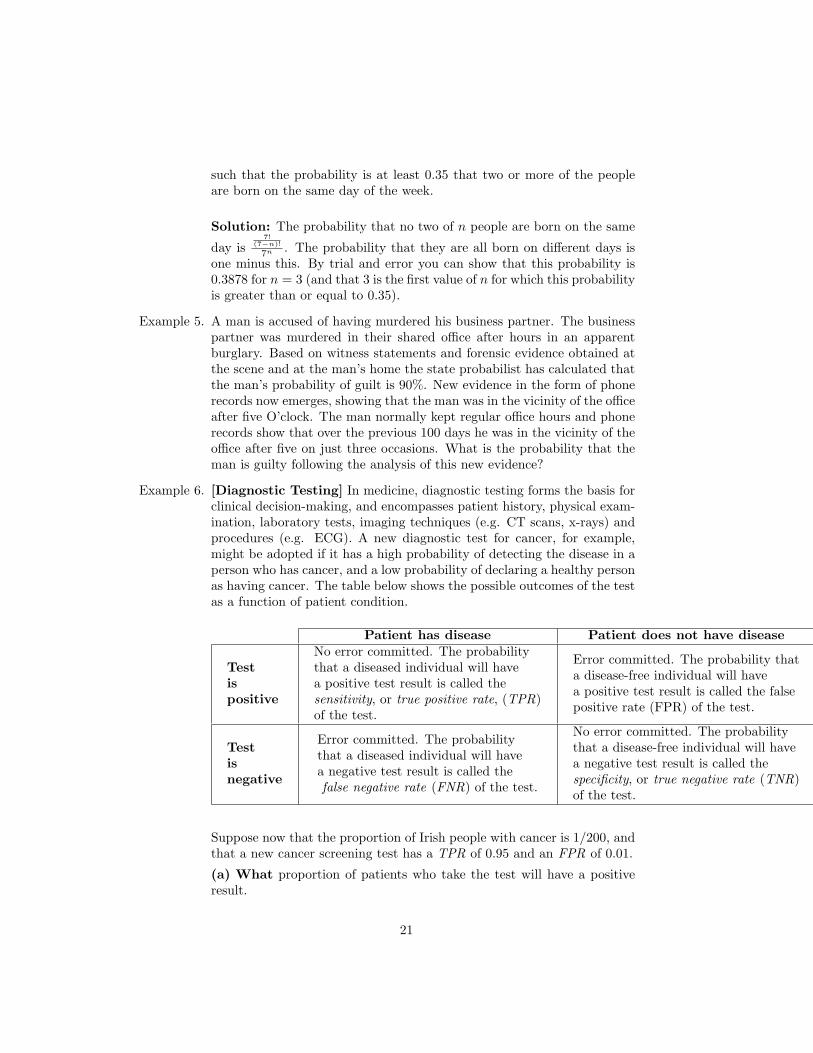
Example 6. [Diagnostic Testing] In medicine, diagnostic testing forms the basis forclinical decision-making, and encompasses patient history, physical exam-ination, laboratory tests, imaging techniques (e.g. CT scans, x-rays) andprocedures (e.g. ECG). A new diagnostic test for cancer, for example,might be adopted if it has a high probability of detecting the disease in aperson who has cancer, and a low probability of declaring a healthy personas having cancer. The table below shows the possible outcomes of the testas a function of patient condition.

Patient has disease Patient does not have disease

Testispositive

No error committed. The probabilitythat a diseased individual will havea positive test result is called thesensitivity, or true positive rate, (TPR)of the test.

Error committed. The probability thata disease-free individual will havea positive test result is called the falsepositive rate (FPR) of the test.

Testisnegative

Error committed. The probabilitythat a diseased individual will havea negative test result is called thefalse negative rate (FNR) of the test.

No error committed. The probabilitythat a disease-free individual will havea negative test result is called thespecificity, or true negative rate (TNR)of the test.

Suppose now that the proportion of Irish people with cancer is 1/200, andthat a new cancer screening test has a TPR of 0.95 and an FPR of 0.01.

(a) What proportion of patients who take the test will have a positiveresult.

21

(b) Given that a patient has a positive result, what is the probabilitythat he/she has cancer?

[Answer : Using formula 15) on Some Useful Formulae in Probability, weget

(a) 1200 × 0.95 + 199

200 × 0.01,while for b) we use Bayes’ Formula (i.e. 16) on

Some Useful Formulae in Probability) to get1

200×0.95

answer in a) .]

6. Box A contains two gold coins, Box B contains two silver coins, and BoxC contains one gold and one silver coin. A box is chosen at random anda coin selected from it. If the selected coin is Gold, what is the prob-ability that the other coin in the selected box is Gold (i.e. what is theprobability that the selection was made from Box A?) [Answer: UsingBayes’ Formula (or use a tree diagram or Venn diagram), we get answer

13×1

13×1+ 1

3×0+ 13×

12

= 23 .

Note: Many people think that the answer to this problem should be 12 .

This misses the point that if we selected a gold coin it is in fact more likelythat we were drawing from A than from C.

7. Birthdays Suppose that there are r randomly selected individuals in aroom. What is the probability that at least two of them have the samebirthday (i.e. born on the same month and day)?

[Note: Ignore leap years, so assume 365 days in a year, and assume thateach person has a probability of 1

365 of being born on any particular day.]

Solution: P (at least two have same birthday) = 1−P (no two have samebirthday) =

1−P

1st personis born onany day

and

2nd personis born on a day

differentfrom the first

and . . . and

rth personis born on a daydifferent from

the previous r − 1

=

by independence

1−P

1st personis born onany day

P

2nd person

is born on a daydifferent

from the first

×...× P

rth person

is born on a daydifferent fromprevious r − 1

= 1− 365

365× 364

365× ...×

365− r + 1365

.

That is, if we let pr be the probability that at least two of r people have

the same birthday, then pr = 1− 365365

× 364365

×

...×365− r + 1

365(*)

22

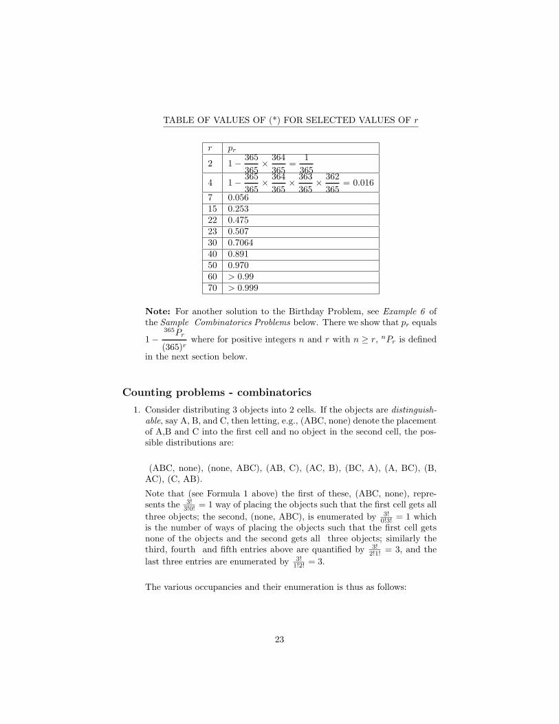
TABLE OF VALUES OF (*) FOR SELECTED VALUES OF r

r pr

2 1− 365365

× 364365

=1

3654 1− 365

365× 364

365× 363

365× 362

365= 0.016

7 0.05615 0.25322 0.47523 0.50730 0.706440 0.89150 0.97060 > 0.9970 > 0.999

Note: For another solution to the Birthday Problem, see Example 6 ofthe Sample Combinatorics Problems below. There we show that pr equals

1−365Pr

(365)rwhere for positive integers n and r with n ≥ r, nPr is defined

in the next section below.

Counting problems - combinatorics

1. Consider distributing 3 objects into 2 cells. If the objects are distinguish-able, say A, B, and C, then letting, e.g., (ABC, none) denote the placementof A,B and C into the first cell and no object in the second cell, the pos-sible distributions are:

(ABC, none), (none, ABC), (AB, C), (AC, B), (BC, A), (A, BC), (B,AC), (C, AB).

Note that (see Formula 1 above) the first of these, (ABC, none), repre-sents the 3!

3!0! = 1 way of placing the objects such that the first cell gets allthree objects; the second, (none, ABC), is enumerated by 3!

0!3! = 1 whichis the number of ways of placing the objects such that the first cell getsnone of the objects and the second gets all three objects; similarly thethird, fourth and fifth entries above are quantified by 3!

2!1! = 3, and thelast three entries are enumerated by 3!

1!2! = 3.

The various occupancies and their enumeration is thus as follows:

23

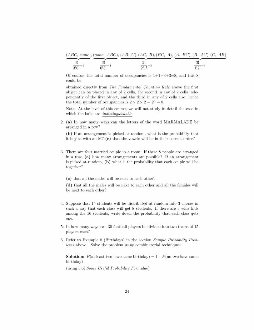
(ABC, none)︸ ︷︷ ︸3!

3!0!=1

, (none, ABC)︸ ︷︷ ︸3!

0!3!=1

, (AB, C), (AC, B), (BC, A)︸ ︷︷ ︸3!

2!1!=3

, (A, BC), (B, AC), (C, AB)︸ ︷︷ ︸3!

1!2!=3

Of course, the total number of occupancies is 1+1+3+3=8, and this 8could be

obtained directly from The Fundamental Counting Rule above the firstobject can be placed in any of 2 cells, the second in any of 2 cells inde-pendently of the first object, and the third in any of 2 cells also; hencethe total number of occupancies is 2× 2× 2 = 23 = 8.

Note: At the level of this course, we will not study in detail the case inwhich the balls are indistinguishable.

2. (a) In how many ways can the letters of the word MARMALADE bearranged in a row?

(b) If an arrangement is picked at random, what is the probability thatit begins with an M? (c) that the vowels will be in their correct order?

3. There are four married couple in a room. If these 8 people are arrangedin a row, (a) how many arrangements are possible? If an arrangementis picked at random, (b) what is the probability that each couple will betogether?

(c) that all the males will be next to each other?

(d) that all the males will be next to each other and all the females willbe next to each other?

4. Suppose that 15 students will be distributed at random into 3 classes insuch a way that each class will get 8 students. If there are 3 whiz kidsamong the 16 students, write down the probability that each class getsone.

5. In how many ways can 30 football players be divided into two teams of 15players each?

6. Refer to Example 8 (Birthdays) in the section Sample Probability Prob-lems above. Solve the problem using combinatorial techniques.

Solution: P (at least two have same birthday) = 1−P (no two have samebirthday)

(using 5.of Some Useful Probability Formulae)

24

= 1− # of groups of r different days that can be chosen from 365 days# of groups of r days that can be taken from 365 days = 1−

365Pr

(365)r

Note that this answer is the same as that given in (*) of the solution toExample 8 in the section Sample Probability Problems above because

1 −365Pr

(365)r= 1 −

(365)!(365−r)!

(365)r= 1 −

365× 364× ...× (365− r + 1)

(365)r= 1 −

365365

× 364365

× ...×365− r + 1

365

Note also that in our derivation above, we used 365Pr and not(365r

)because

the order within each group of r birthdays is important (compare 3 and4 in the Useful Combinatorial Formulae section above). For example, ifyou have a birthday on January 1 and I have birthday on January 2, thatis quite a different event than you having birthday on January 2 and mehaving birthday on January 1.

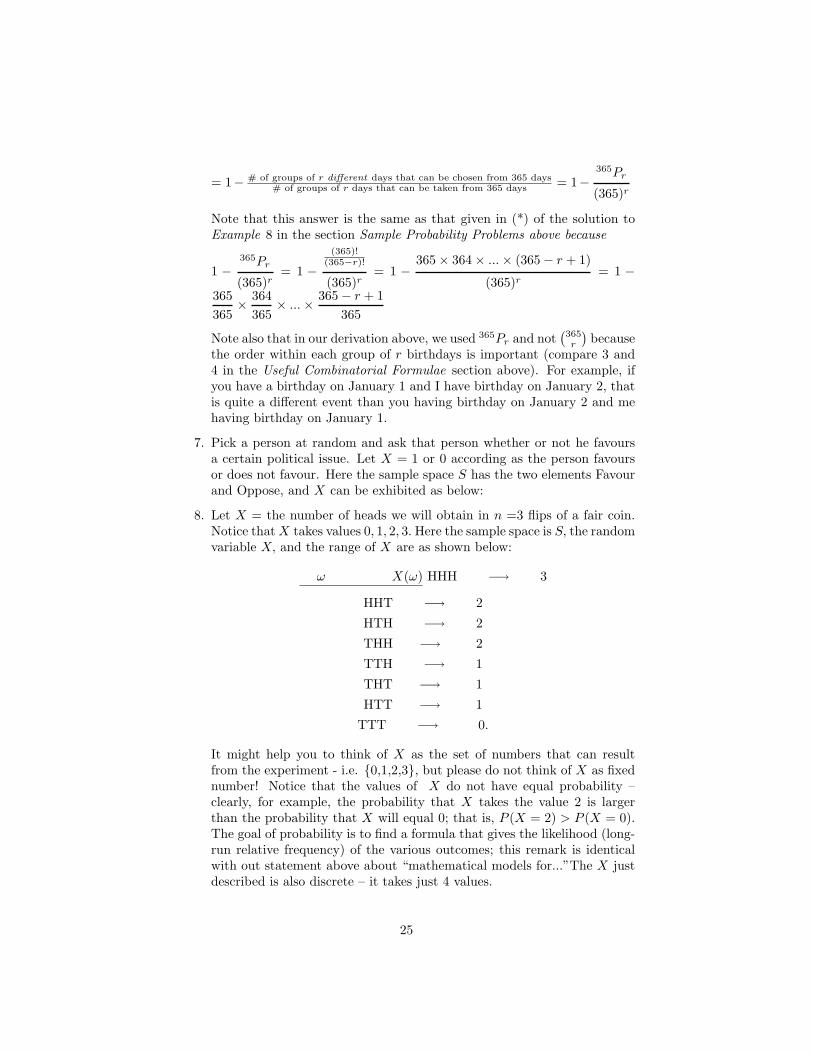
7. Pick a person at random and ask that person whether or not he favoursa certain political issue. Let X = 1 or 0 according as the person favoursor does not favour. Here the sample space S has the two elements Favourand Oppose, and X can be exhibited as below:

8. Let X = the number of heads we will obtain in n =3 flips of a fair coin.Notice that X takes values 0, 1, 2, 3. Here the sample space is S, the randomvariable X, and the range of X are as shown below:

ω X(ω) HHH −→ 3

HHT −→ 2

HTH −→ 2

THH −→ 2

TTH −→ 1

THT −→ 1

HTT −→ 1

TTT −→ 0.

It might help you to think of X as the set of numbers that can resultfrom the experiment - i.e. 0,1,2,3, but please do not think of X as fixednumber! Notice that the values of X do not have equal probability –clearly, for example, the probability that X takes the value 2 is largerthan the probability that X will equal 0; that is, P (X = 2) > P (X = 0).The goal of probability is to find a formula that gives the likelihood (long-run relative frequency) of the various outcomes; this remark is identicalwith out statement above about “mathematical models for...”The X justdescribed is also discrete – it takes just 4 values.

25

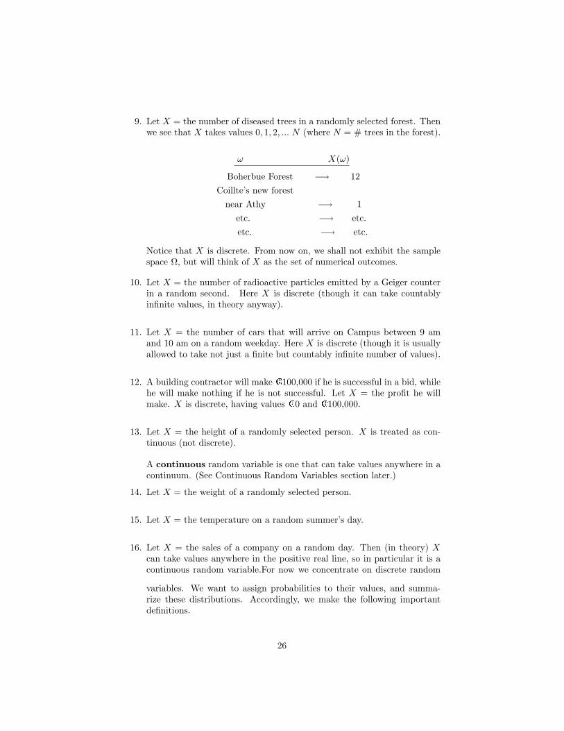
9. Let X = the number of diseased trees in a randomly selected forest. Thenwe see that X takes values 0, 1, 2, ... N (where N = # trees in the forest).

ω X(ω)

Boherbue Forest −→ 12Coillte’s new forest

near Athy −→ 1etc. −→ etc.etc. −→ etc.

Notice that X is discrete. From now on, we shall not exhibit the samplespace Ω, but will think of X as the set of numerical outcomes.

10. Let X = the number of radioactive particles emitted by a Geiger counterin a random second. Here X is discrete (though it can take countablyinfinite values, in theory anyway).

11. Let X = the number of cars that will arrive on Campus between 9 amand 10 am on a random weekday. Here X is discrete (though it is usuallyallowed to take not just a finite but countably infinite number of values).

12. A building contractor will make ¿100,000 if he is successful in a bid, whilehe will make nothing if he is not successful. Let X = the profit he willmake. X is discrete, having values ¿0 and ¿100,000.

13. Let X = the height of a randomly selected person. X is treated as con-tinuous (not discrete).

A continuous random variable is one that can take values anywhere in acontinuum. (See Continuous Random Variables section later.)

14. Let X = the weight of a randomly selected person.

15. Let X = the temperature on a random summer’s day.

16. Let X = the sales of a company on a random day. Then (in theory) Xcan take values anywhere in the positive real line, so in particular it is acontinuous random variable.For now we concentrate on discrete random

variables. We want to assign probabilities to their values, and summa-rize these distributions. Accordingly, we make the following importantdefinitions.

26

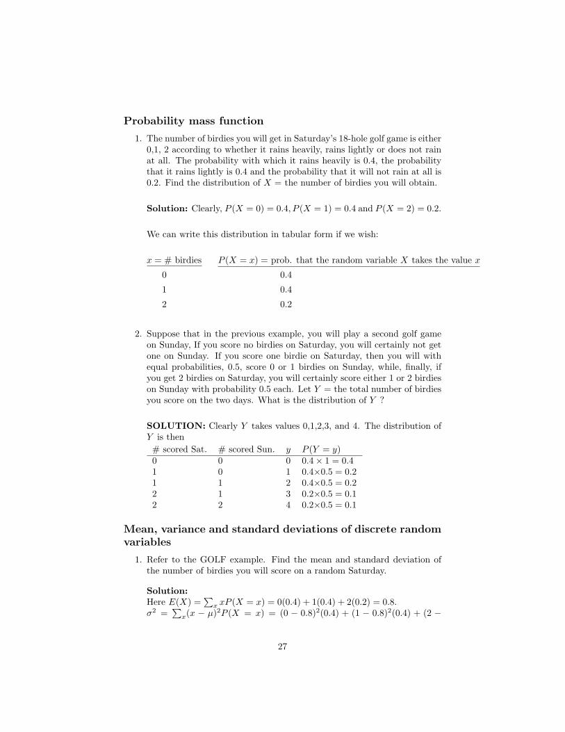
Probability mass function

1. The number of birdies you will get in Saturday’s 18-hole golf game is either0,1, 2 according to whether it rains heavily, rains lightly or does not rainat all. The probability with which it rains heavily is 0.4, the probabilitythat it rains lightly is 0.4 and the probability that it will not rain at all is0.2. Find the distribution of X = the number of birdies you will obtain.

Solution: Clearly, P (X = 0) = 0.4, P (X = 1) = 0.4 and P (X = 2) = 0.2.

We can write this distribution in tabular form if we wish:

x = # birdies P (X = x) = prob. that the random variable X takes the value x

0 0.4

1 0.4

2 0.2

2. Suppose that in the previous example, you will play a second golf gameon Sunday, If you score no birdies on Saturday, you will certainly not getone on Sunday. If you score one birdie on Saturday, then you will withequal probabilities, 0.5, score 0 or 1 birdies on Sunday, while, finally, ifyou get 2 birdies on Saturday, you will certainly score either 1 or 2 birdieson Sunday with probability 0.5 each. Let Y = the total number of birdiesyou score on the two days. What is the distribution of Y ?

SOLUTION: Clearly Y takes values 0,1,2,3, and 4. The distribution ofY is then# scored Sat. # scored Sun. y P (Y = y)0 0 0 0.4× 1 = 0.41 0 1 0.4×0.5 = 0.21 1 2 0.4×0.5 = 0.22 1 3 0.2×0.5 = 0.12 2 4 0.2×0.5 = 0.1

Mean, variance and standard deviations of discrete randomvariables

1. Refer to the GOLF example. Find the mean and standard deviation ofthe number of birdies you will score on a random Saturday.

Solution:Here E(X) =

∑x xP (X = x) = 0(0.4) + 1(0.4) + 2(0.2) = 0.8.

σ2 =∑

x(x − µ)2P (X = x) = (0 − 0.8)2(0.4) + (1 − 0.8)2(0.4) + (2 −

27

0.8)2(0.2) = 0.256 + 0.016 + 0.288 = 0.56. Hence the standard deviationof X is σ =

√0.56 = 0.7483.

There is another formula, which is often a more convenient way of calcu-lating the variance: ∑

x

x2P (X = x)− µ2forσ2

In this case we would obtain σ2 = (0)2(0.4)+(1)2(0.4)+(2)2(0.2)−(0.8)2 =1.2− 0.64 = 0.56,

and hence σ =√

0.56 = 0.7483 as above.]

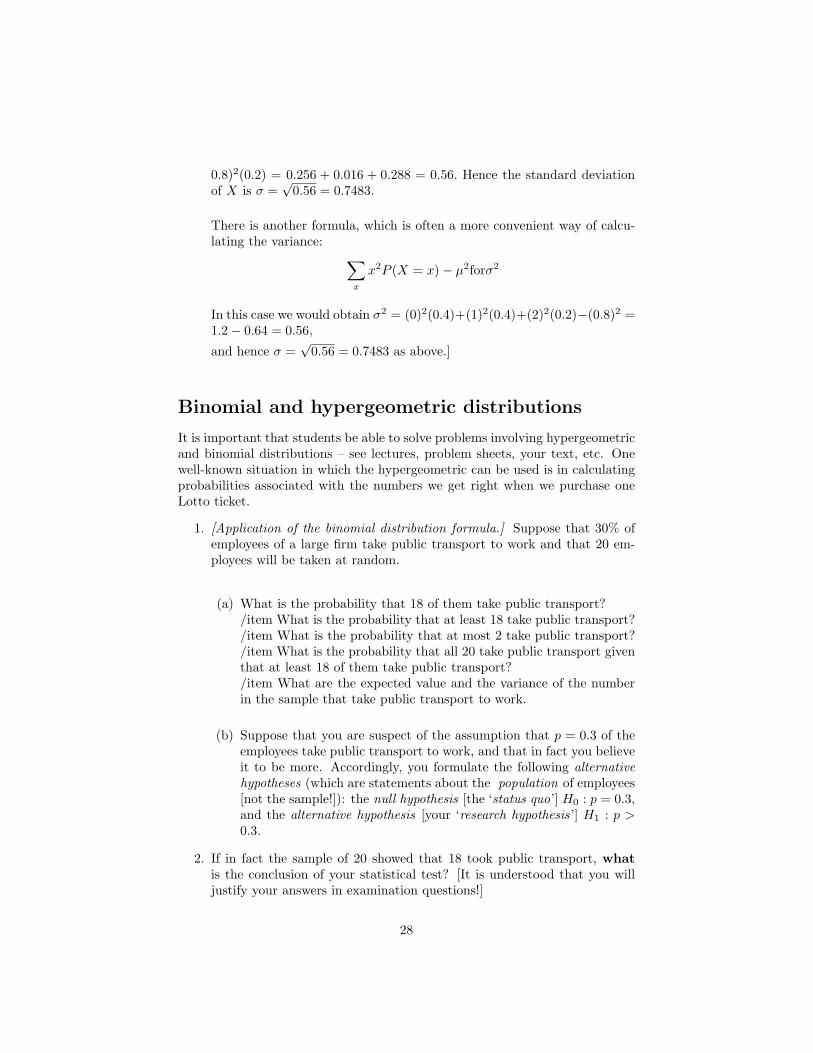
Binomial and hypergeometric distributions

It is important that students be able to solve problems involving hypergeometricand binomial distributions – see lectures, problem sheets, your text, etc. Onewell-known situation in which the hypergeometric can be used is in calculatingprobabilities associated with the numbers we get right when we purchase oneLotto ticket.

1. [Application of the binomial distribution formula.] Suppose that 30% ofemployees of a large firm take public transport to work and that 20 em-ployees will be taken at random.

(a) What is the probability that 18 of them take public transport?/item What is the probability that at least 18 take public transport?/item What is the probability that at most 2 take public transport?/item What is the probability that all 20 take public transport giventhat at least 18 of them take public transport?/item What are the expected value and the variance of the numberin the sample that take public transport to work.

(b) Suppose that you are suspect of the assumption that p = 0.3 of theemployees take public transport to work, and that in fact you believeit to be more. Accordingly, you formulate the following alternativehypotheses (which are statements about the population of employees[not the sample!]): the null hypothesis [the ‘status quo’] H0 : p = 0.3,and the alternative hypothesis [your ‘research hypothesis’] H1 : p >0.3.

2. If in fact the sample of 20 showed that 18 took public transport, whatis the conclusion of your statistical test? [It is understood that you willjustify your answers in examination questions!]

28

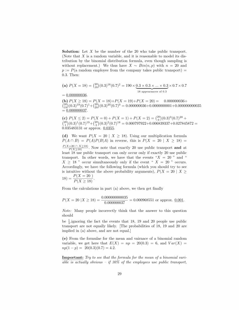
Solution: Let X be the number of the 20 who take public transport.(Note that X is a random variable, and it is reasonable to model its dis-tribution by the binomial distribution formula, even though sampling iswithout replacement.) We thus have X ∼ Bin(n, p) with n = 20 andp := P (a random employee from the company takes public transport) =0.3. Then:

(a) P (X = 18) =(2018

)(0.3)18(0.7)2 = 190× 0.3× 0.3× ...× 0.3︸ ︷︷ ︸

18 appearances of 0.3

× 0.7× 0.7

= 0.000000036.

(b) P (X ≥ 18) = P (X = 18)+P (X = 19)+P (X = 20) = 0.000000036+(2019

)(0.3)19(0.7)1+

(2020

)(0.3)20(0.7)0 = 0.000000036+0.0000000001+0.000000000035

= 0.000000037.

(c) P (X ≤ 2) = P (X = 0) + P (X = 1) + P (X = 2) =(200

)(0.3)0(0.7)20 +(

201

)(0.3)1(0.7)19+

(202

)(0.3)2(0.7)18 = 0.000797922+0.006839337+0.027845872 =

0.035483131 or approx. 0.0355.

(d) We want P (X = 20 | X ≥ 18). Using our multiplication formulaP (A ∩ B) = P (A)P (B|A) in reverse, this is P (X = 20 | X ≥ 18) =P (X=20 ∩ X≥18)

P (X≥18) . Now note that exactly 20 use public transport and atleast 18 use public transport can only occur only if exactly 20 use publictransport. In other words, we have that the events “X = 20 ” and “X ≥ 18 ” occur simultaneously only if the event “ X = 20 ” occurs.Accordingly, we have the following formula (which you should try to seeis intuitive without the above probability arguments), P (X = 20 | X ≥

18) =P (X = 20 )P (X ≥ 18)

.

From the calculations in part (a) above, we then get finally

P (X = 20 |X ≥ 18) =0.000000000035

0.000000037= 0.000968551 or approx. 0.001.

Note: Many people incorrectly think that the answer to this questionshould

be 13 ,ignoring the fact the events that 18, 19 and 20 people use public

transport are not equally likely. [The probabilities of 18, 19 and 20 areimplied in (a) above, and are not equal.]

(e) From the formulae for the mean and vairnace of a binomial randomvariable, we get here that E(X) = np = 20(0.3) = 6, and V ar(X) =np(1− p) = 20(0.3)(0.7) = 4.2.

Important: Try to see that the formula for the mean of a binomial vari-able is actually obvious – if 30% of the employees use public transport,

29

then in a random sample of 20, you’d expect 20×0.3 = 6 to be usingpublic transport. The interpretation of the mean and variance of any ran-dom variable are similar to those given in the context of Lotto winningsin Problem 3 below. Ensure that you understand them.

(f) We would conclude that p > 0.3. Why? Well, if the null hypothesisH0 was true, then only 30% of employees use public transport. For arandom sample of 20 employees, we showed in (b) above that under thisnull hypothesis (i.e. if this null hypothesis is true), the chance of observing18 or more taking public transport is only 0.000000037, or about 1 chancein 27 million! This is a very small probability, so either a very very rareevent occurred, or our H0 is false.

It is reasonable then to reject the null hypothesis and conclude H1. [If youdo not understand this, note that all that is being said is that if only 30%of the population use public transport, it would be very unlikely to get asample result at least as extreme as we got. Notice that if p > .3, e.g. ifp = .9, then the sample result of 18 would not be unlikely. It makes sensethen to conclude that p exceeds 0.3.]

USEFUL NOTE : In any significance testing problem the p-value ofthe statistical test is the probability of obtaining a sample re-sult at least as extreme as that which we did observe, whenthe null hypothesis is true. If this p-value is deemed ‘too small’, thenwe say that our sample result (= 18 in the above example) is statisticallysignificant, and we reject the null hypothesis.

[Note: You should practice other binomial problems. For example, startwith something like: suppose that 1% of screws produced in a manufactur-ing process are defective; suppose that 51% of births are females; supposethat 60% of items sold in a store are priced at more than £20 and soon. Then in a random sample that will be taken, work out answers toquestions similar to those in (a) – (e) above.]

3. Let X be a discrete random variable. Prove that the two formulas youhave seen for V ar(X) are identical.

Solution:

We must prove that∑

x(x− µ)2P (X = x) =∑

x x2P (X = x)− µ2.

This follows from the following calculation:∑x(x− µ)2P (X = x) =

∑x(x2 + µ2 − 2µx)P (X = x) =

why?∑x x2P (X = x) +

∑x µ2P (X = x)−

∑x 2µxP (X = x) =

30

∑x x2P (X = x) + µ2

∑x P (X = x)− 2µ

∑x xP (X = x)

[since constants can be taken outside summations]

=∑

x x2P (X = x) + µ2 (1)− 2µ(µ) [since∑

x P (X = x) = 1 (why?)

Poisson process

1. Suppose that the number of goals in a random Celtic football game has aPoisson distribution with, on average, 2 goals per game. Find the proba-bility of

(a) one goal in the next game,

(b) at least one goal in the next game,

(c) one goal in the next two games.

Solution: In (*), we put α = 2 throughout the question. Let X =the number of goals scored in one random game. Then (a) P (X =

1) =put t=1 and x=1 in (*)

e−2 (2)1

1!= 2e−2.

(This is approximately 0.2707 using a calculator.)

(b) P (X ≥ 1) =(working with the complement saves much work)

1−P (X = 0) =put t=1 and x=0 in (*)

1− e−2 (2)0

0!= 1− e−2 . ‘ Now let Y = the number of goals scored in the

next two games. Then

(c) P (Y = 1) =put t=2 and x=1 in (*)

e−4 (4)1

1!= 4e−4 .

[Note: This result could have been derived by partitioning as in formula(15) of Useful Probability Formulae, as follows. P (one goal in the next twogames) = P (one goal in the first game and no goal in the second game) +

P (no goal in the first game and one goal in the second game)

=by independence – see (A3)

P (one goal in the first game)P (no goal in the sec-

ond game) +

P (no goal in the first game)P ( one goal in the second game) =using (*) with α=2, t=1, and x=0, 1

e−2 (2)1

1!e−2 (2)0

0!+ e−2 (2)0

0!e−2 (2)1

1!= 4e−4, as above.

31

2. In the last example, calculate the probability that two goals will be scoredin the next game given that at least one goal will be scored.

Solution: We require

P (X = 2 |X ≥ 1) =multiplication formula

P (X = 2 ∩ X ≥ 1)P (X ≥ 1)

=why?

P (X = 2)P (X ≥ 1)

=

P (X = 2)1− P (X = 0)

=using (*)

e−2 (2)2

2!

1− e−2(2)0

0!

=2

e2 − 1.

Poisson approximation to the Binomial

1. Suppose that 1% of screws produced in a factory are defective. If 100screws are selected at random, what is the (a) exact and (b) approximateprobability that 5 of them will be defective.

Solution: Let X = the number of defectives in the random sample ofn = 100.

We require P (X = 5).

(a) Using the binomial distribution function P (X = x) =(nx

)θx(1−θ)n−x,

x = 0, 1, 2, ..., n

with n = 100, θ = P (a random bolt is defective) = 0.01, and x = 5, wehave P (X = 5) =

(1005

)(0.01)5(1− 0.01)95 = 0.0029.

(b) Using the Poisson approximation to the binomial ) we use the formula(*) with λ = αt = expected number of defectives in the sample = θn =(0.01)100 = 1.

Then P (X = 5) $ e−1 (1)5

5!= 0.0031.

(Notice how close the two answers are, but how much easier the Poissonis.)

Normal random variables

1. Suppose that heights of people have a normal distribution with meanµ = 68 and standard deviation σ = 3. (a) What proportion of people haveheights above 71? (b) What proportion of people have heights below 62?(c) If 2.5% of people have heights above a, what is a?

Solution: Let X = height of a random person. Then we are given thatX v N(µ, σ2) with µ = 68 and σ = 3.

32

(a) We want P (X > 71). Using the standardization formula (*) above, we

find that this is P (X > 71) = P (X − µ

σ>

71− µ

σ) = P (Z >

71− 683

) =

P (Z > 1) = 0.1587. Here, and elsewhere unless stated otherwise, Z de-notes a N(0, 1) random variable, and we have used standard normal tablesto get the number 0.1587.

(b) Similarly, P (X < 62) = P (Z < −2) =by symmetry

P (Z > 2) = 0.0228.

(c) We want a so that P (X > a) = 0.025. (Notice that this is just areversal of the type of question in (b) above.

Standardizing, we have P (Z >a− 68

3) = 0.025. Hence form N(0, 1) ta-

bles, or the information in the question, we geta− 68

3= 1.96. Hence

a = 68 + 3× 1.96 = 73.88.

Central Limit Theorem

1. Refer to our “heights” example above. Suppose that 100 people will beselected at random. What is the probability that their mean height Xwill exceed 71?

Solution: We require P (X > 71). From the above theorem, X vN(µ, σ2

n ), so we just apply our standardization procedure (*). We get

P (X > 71) = P (X − µ

σ/√

n>

71− µ

σ/√

n) = P (Z >

71− 683/√

100) = P (Z > 10) $ 0.

(Note that we cannot find the number 10 in our z-tables, but the tablesgive the area above 3.09 to be about 0.001, so the area above 10 must beextremely close to 0.)

Note that by the Central Limit Theorem, it was not necessary to knowthat the distribution of the population was normal. this is because ourcalculation relied on knowledge of the distribution of X, and the CentralLimit Theorem says that this distribution is approximately normal any-way, since the sample size n is large. Thus the answer we obtained wouldbe approximately correct anyway.

2. Refer again to our HEIGHTS examples above. Suppose that µ is actuallyunknown. In estimating µ, would you prefer to use the value x of onerandom person’s height X, or the value x of the mean X of 100 randomlyselected peoples’ heights?

Solution: Intuitively, you’d prefer to use the mean x (surely, the moreobservations you take from a population, the more information we obtainabout some unknown aspect of this population!) But let’s answer thequestion rigorously. The distribution of each of X and X are normalwith the same mean µ (the population mean). But while X has standarddeviation σ = 3, X has standard deviation σ√

n= 3√

100= 0.3. This means

33

that we are much more likely to get a value of X “close” to µ than we are ofgetting a value of X “close” to µ. Here is another more mathematical wayof providing an answer: First note that from standard normal distributiontables, we see that if we have a standard normal variable Z, then P (−1 <Z < 1) = 0.6826, P (−2 < Z < 2) = 0.9544, P (−2 < Z < 2) = 0.9987.These numbers are useful to remember, and state that about 68%, 95%,and practically all, values of a normal variable lie within, ± one standarddeviation, ±two standard deviations, and ±three standard deviations ofthe mean of the variable. Hence [see the standardization formula (*)above], since X−µ

σ and X−µσ/√

neach have the standard normal distribution,

we find for example that P (−1 < X−µσ < 1) = 0.6826 and P (−1 < X−µ

σ/√

n<

1) = 0.6826. That is, P (−σ < X − µ < σ) = 0.6826 and P (−σ/√

n <X−µ < σ/

√n) = 0.6826, i.e. (since, in our example, σ = 3 and n = 100),

P (−3 < X − µ < 3) = 0.6826 and P (−0.3 < X − µ < 0.3) = 0.6826.We thus see that with probability approx. 0.68, X will lie within only adistance 3 of µ, while with probability approx. 0.68, X will be within 0.3of µ. This confirms our preference for using X rather than one randomobservation X. Also check that the bigger the sample size, the more likelyit is that X will lie within any given distance of µ (replace n = 100 by,e.g., n = 1, 000 above).

Sampling methods

1. It is desired to take a sample of 100 students from an university that has10, 000 students. Suppose we divide the population into two strata, malesand females, and that there are 6, 000 male students and 4, 000 femalestudents in the university. How many of each sex should be included inthe sample of 100 if we use proportional allocation?

Solution: We would take 100 × 600010000 = 60 males and 100 × 4000

10000 = 40females.

2. Refer to the last example and suppose that the survey of 100 studentsis to be conducted to estimate the mean annual consumption, µ, of beerby students at NUI, Galway. Suppose that the standard deviation of thenumber of units of beer consumed by males and females are σ1 = 100 andσ2 = 50, respectively. [Note: If these standard deviations were unknown,we’d estimate them by the sample standard deviations got from a pilotstudy, or by some other method.] How many students from each stratumshould be taken if optimal allocation is used?

Solution: The number of males we should sample is

100× 6000×1006000×100+4000×50 = 75

and the number of females will equal

34

100× 4000×506000×100+4000×50 = 25

[this 25 could more easily be obtained by subtracting 75 from the totalsample size of 100].

3. Refer to the last example. Suppose that the mean number of units ofalcohol consumed by the 75 males in the past year turned out to be x1 =800 and that the mean for the 25 females was x2 = 100. What is the bestestimate of µ?

Solution:75× 800 + 25× 100

75 + 25= 625.

Note that this is a weighted average,n1n x1+ n2

n x2 = 75100×800+ 25

100×100 =625, of the two sample means 800 and 100, with weights given by theproportions of males ( 75

100 ) and females ( 25100 ) in the sample of 100. If you

have difficulty with this, note that we would estimate µ by means of thesample mean number of units drank. This sample mean is of course

total number of units drank by the 100 students in the sampletotal number of students in the sample =

total number of units drank by the 75 males + total number of units drank by the 25 females100 =

75×800+25×100100 = 625.

It is important to note that the correct answer is not the ordinary average800+100

100 = 450 of the numbers 800 and 100.

Sampling distributions

The purpose of the following long exercise is to give you an intuitive feelingfor how sample means and sample standard deviations relate to the populationmean and standard deviation. Some students may find this exercise very helpful,others less so. If you do not find it is helping you to improve your understandingof this topic you can skip it.

Recall that statistics is primarily concerned with making valid inferences aboutpopulations based on information contained in samples taken from these popu-lations. In this sheet, we will examine some ideas that are key throughout thecourse in estimating unknown population parameters from the values of samplestatistics. For illustrative purposes, we will take a known population, but notethat in practise this will not be the case.Consider the following population consisting of the 3 elements: 1, 2, 3.We first calculate the mean and variance of the population.The mean and variance are got using the following general formulae for themean and variance of any finite population y1, y2, ..., yN:

Population mean := µ = 1N

∑Ni=1 yi (1)

35

We get µ = 13 (1 + 2 + 3) = 2 (2)

Also, we have the following formula for the variance of any finite populationy1, y2, ..., yN:Population variance := σ2 = 1

N

∑Ni=1(yi − µ)2 (3)

We thus obtain σ2 = 13

[(1− 2)2 + (2− 2)2 + (3− 2)2

]= 2

3 (4)Alternatively and equivalently, we can imagine a random variable X takingvalues 1,2 and 3 with probabilities

P (X = x) =13, x = 1, 2, 3.

This distribution is shown in table form below.

TABLE 1x P (X = x)1 1/32 3/33 1/3

Then note that the above population is equivalent to this random variable andits distribution. Then using the following formula for the mean (i.e. the expectedvalue) of any discrete random variable Y

E(Y ) =∑

yP (Y = y) (5)

We getµ = E(X) = 1× 1

3 + 2× 13 + 3× 1

3 = 2 (6)agreeing with (2).

Also, we obtain the variance of X by using either of the following formulae forthe variance of any discrete random variable Y :

σ2 = V ar(Y ) = E(Y − E(Y ))2 =∑

(y − E(Y ))2P (Y = y) (7)We thus get σ2 = V ar(X) = (1− 2)2 × 1

3 + (2− 2)2 × 13 + (3− 2)2 × 1

3 = 23 (8)

agreeing with (4) above.

Remark 2 We could have used another equivalent formula for the variance (3);this equivalent formula is.

V ar(X) = EX2 − E2(X) (9)

which since our X is discrete here, becomes∑x2P (Y = x)− E2(X)

(Check that this again gives 23 in our example).

36

Remark 3 ASIDE: If X was continuous with density f(x), we would haveused the following formulae for the mean and variance:

µ = E(X) =∫

xf(x)dx (10)andσ2 = V ar(X) = E(X − E(X))2 =

∫(x− E(X))2f(x)dx =

EX2 − E2(X) =∫

x2 f(x)dx− µ2 (11)

Remark 4 In all cases, the population standard deviation is always defined asσ = +

√σ2 (12)

We now study samples of size n = 2 taken with replacement from the abovepopulation. Note that in the real world, only one sample is taken (with-

out replacement), but by examining every possible sample, we can getan idea of how good any one sample would be in giving informationabout the population.

The possible samples are: (1,1), (1,2), (2,1), (1,3), (3,1), (2,2,), (2,3), (3,2),(3,3).We will calculate the mean and variance of each sample and construct twodistributions.Note that the mean and variance of any set of numbers x1, x2, ..., xn are, re-spectively,

Sample Mean:= x := 1n

∑ni=1 xi (13)

andSample Variance:= s2 := 1

n−1

∑ni=1(xi − x)2 = 1

n−1

[∑ni=1 x2

i − nx2]

(14)You can try to fill in the following table (a few of the rows are already completed)

TABLE 2Samples Sample mean x Sample variance s2 Sample st. dev. s =

√s2

1, 1 1+12 = 1

12−1(1− 1)2

+(1− 1)2 = 0√

0 = 0

1, 2 1+22 = 1.5

12−1(1− 1.5)2

+(2− 1.5)2 = 12

√12

2, 12, 21, 3 2 2

√2

3, 12, 3 2.5 1

2

√12

3, 23, 3

37

We next calculate the average of all the sample means, and the average of allthe sample variances.Let X be the mean of a random sample, and let S2 be the variance of a randomsample.

We get [using (1)] that the mean of the population of all nine x values isE(X) = 2+1.5+1.5+2+2+2+2.5+2.5+3

9 = 2. (15)

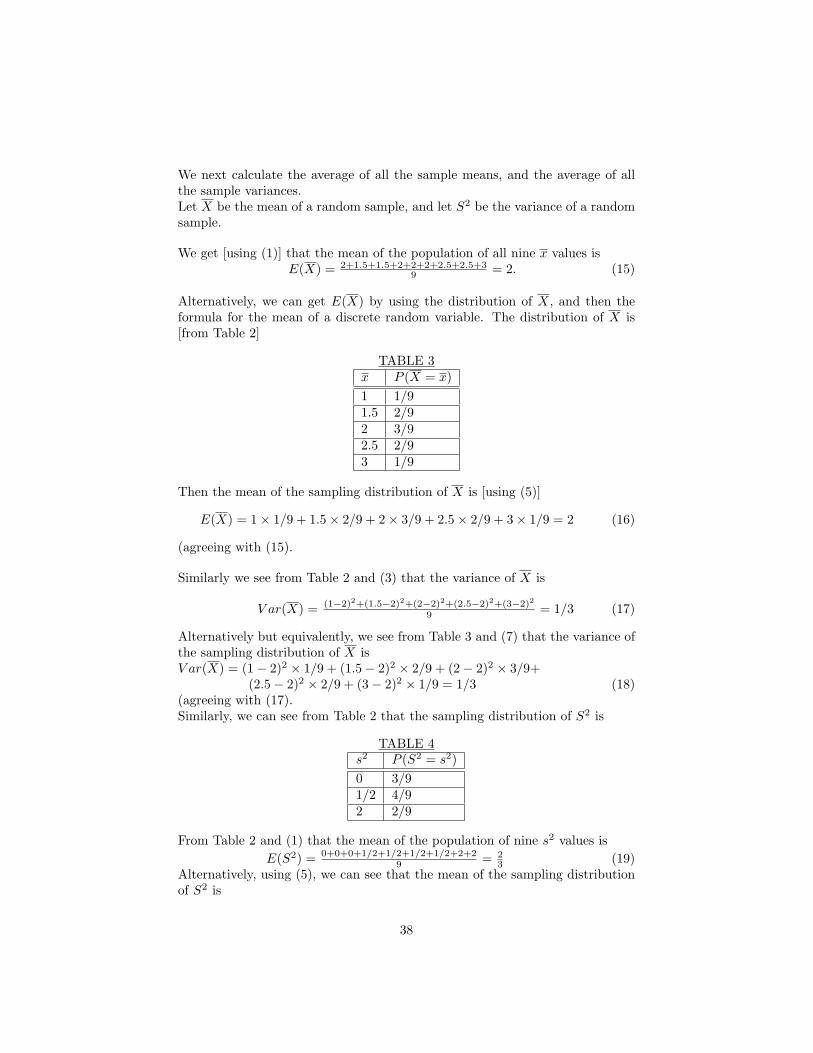
Alternatively, we can get E(X) by using the distribution of X, and then theformula for the mean of a discrete random variable. The distribution of X is[from Table 2]

TABLE 3x P (X = x)1 1/91.5 2/92 3/92.5 2/93 1/9

Then the mean of the sampling distribution of X is [using (5)]

E(X) = 1× 1/9 + 1.5× 2/9 + 2× 3/9 + 2.5× 2/9 + 3× 1/9 = 2 (16)

(agreeing with (15).

Similarly we see from Table 2 and (3) that the variance of X is

V ar(X) = (1−2)2+(1.5−2)2+(2−2)2+(2.5−2)2+(3−2)2

9 = 1/3 (17)

Alternatively but equivalently, we see from Table 3 and (7) that the variance ofthe sampling distribution of X isV ar(X) = (1− 2)2 × 1/9 + (1.5− 2)2 × 2/9 + (2− 2)2 × 3/9+

(2.5− 2)2 × 2/9 + (3− 2)2 × 1/9 = 1/3 (18)(agreeing with (17).Similarly, we can see from Table 2 that the sampling distribution of S2 is

TABLE 4s2 P (S2 = s2)0 3/91/2 4/92 2/9

From Table 2 and (1) that the mean of the population of nine s2 values isE(S2) = 0+0+0+1/2+1/2+1/2+1/2+2+2

9 = 23 (19)

Alternatively, using (5), we can see that the mean of the sampling distributionof S2 is

38

E(S2) = 0× 3/9 + 1/2× 4/9 + 2× 2/9 = 6/9 = 2/3 (20)Alternatively,using (5), we can see that the mean of the sampling distributionof S2 is

E(S2) = 0× 3/9 + 1/2× 4/9 + 2× 2/9 = 6/9 = 2/3 (21)From (15) or (16 ) and (2) or (6), we see that

E(X) = µ (22)that is, the mean of all the sample means is the population mean,i.e. the mean of all the samples means is the populations mean,i.e. the expected value of the random sample mean X is thepopulation mean µ.Also comparing (17) or (18) with (4) or (8) we see that

V ar(X) = σ2/n (23)

That is, the variance of all the sample means is the population variance dividedby the sample size.Finally, notice from (4) or (8) with (20) or (21), we see that

E(S2) = σ2 (24)

Summarizing, we have the following important properties:

Remark 5 (Important general properties of the sample mean X and sample variance S2)If a random sample of size n is taken without replacement from an infinite pop-ulation (or from as finite population when sampling is with replacement) thathas mean µ and variance σ2, then the sample mean X and sample variance S2

satisfyE(X) = µ (25)V ar(X) = σ2/n (26)

and

E(S2) = σ2 (27)

In particular then, X and S2 are unbiased estimators of µ and σ2, respectively.This is because any estimator is said to be an unbiased estimator of a parameterif the mean of the distribution of that estimator is the parameter.

Remark 6 It is helpful to note think of µ and σ as the limit, as the sample sizen tends to ∞, of x and s, respectively.

Remark 7 In practise, we will not know the elements of the population and inparticular will not know the parameters µ and σ2. We are allowed to take onesample from the population. Ask yourself if you think that the sample mean xwould be a good estimate of µ. From (22) or (25) we see that it is unbiased forµ. From (23) you can see that if n is large, the variance of X will decrease. Inparticular, you can see that you’d prefer to take as big a sample size as is feasible

39

(taking cost, time and other considerations into account). Putting this anotherway, you’d be more likely to get a sample mean that is close to the unknown µ ifyou take a big sample size than if you take a small sample size. These pointsare very important!

Normal approximation to the binomial distribution

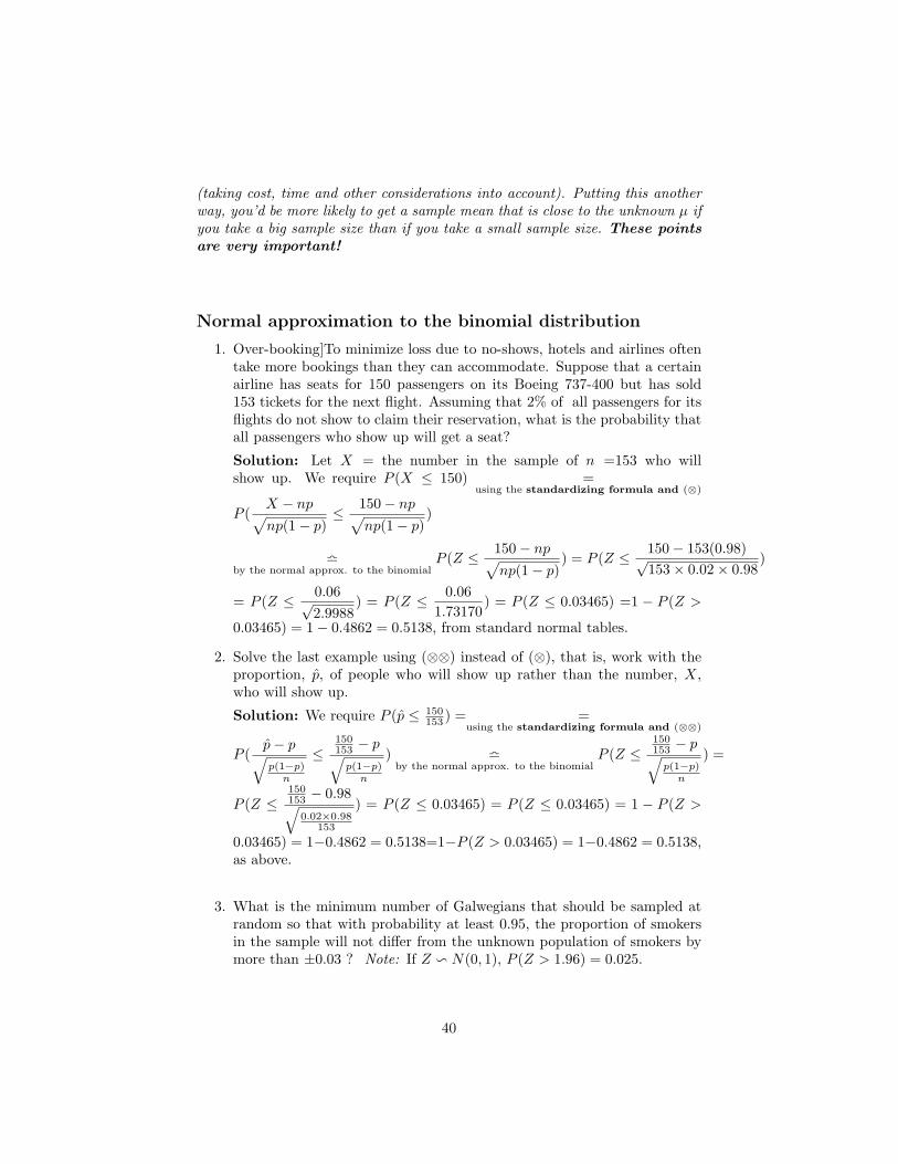
1. Over-booking]To minimize loss due to no-shows, hotels and airlines oftentake more bookings than they can accommodate. Suppose that a certainairline has seats for 150 passengers on its Boeing 737-400 but has sold153 tickets for the next flight. Assuming that 2% of all passengers for itsflights do not show to claim their reservation, what is the probability thatall passengers who show up will get a seat?

Solution: Let X = the number in the sample of n =153 who willshow up. We require P (X ≤ 150) =

using the standardizing formula and (⊗)

P (X − np√np(1− p)

≤ 150− np√np(1− p)

)

lby the normal approx. to the binomial

P (Z ≤ 150− np√np(1− p)

) = P (Z ≤ 150− 153(0.98)√153× 0.02× 0.98

)

= P (Z ≤ 0.06√2.9988

) = P (Z ≤ 0.061.73170

) = P (Z ≤ 0.03465) =1 − P (Z >

0.03465) = 1− 0.4862 = 0.5138, from standard normal tables.

2. Solve the last example using (⊗⊗) instead of (⊗), that is, work with theproportion, p, of people who will show up rather than the number, X,who will show up.

Solution: We require P (p ≤ 150153 ) = =

using the standardizing formula and (⊗⊗)

P (p− p√p(1−p)

n

≤150153 − p√

p(1−p)n

) lby the normal approx. to the binomial

P (Z ≤150153 − p√

p(1−p)n

) =

P (Z ≤150153 − 0.98√

0.02×0.98153

) = P (Z ≤ 0.03465) = P (Z ≤ 0.03465) = 1 − P (Z >

0.03465) = 1−0.4862 = 0.5138=1−P (Z > 0.03465) = 1−0.4862 = 0.5138,as above.

3. What is the minimum number of Galwegians that should be sampled atrandom so that with probability at least 0.95, the proportion of smokersin the sample will not differ from the unknown population of smokers bymore than ±0.03 ? Note: If Z v N(0, 1), P (Z > 1.96) = 0.025.

40

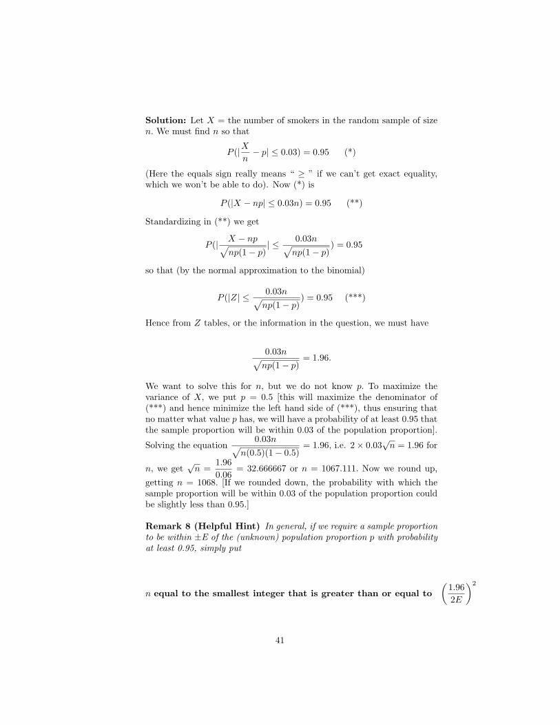
Solution: Let X = the number of smokers in the random sample of sizen. We must find n so that

P (|Xn− p| ≤ 0.03) = 0.95 (*)

(Here the equals sign really means “ ≥ ” if we can’t get exact equality,which we won’t be able to do). Now (*) is

P (|X − np| ≤ 0.03n) = 0.95 (**)

Standardizing in (**) we get

P (| X − np√np(1− p)

| ≤ 0.03n√np(1− p)

) = 0.95

so that (by the normal approximation to the binomial)

P (|Z| ≤ 0.03n√np(1− p)

) = 0.95 (***)

Hence from Z tables, or the information in the question, we must have

0.03n√np(1− p)

= 1.96.

We want to solve this for n, but we do not know p. To maximize thevariance of X, we put p = 0.5 [this will maximize the denominator of(***) and hence minimize the left hand side of (***), thus ensuring thatno matter what value p has, we will have a probability of at least 0.95 thatthe sample proportion will be within 0.03 of the population proportion].

Solving the equation0.03n√

n(0.5)(1− 0.5)= 1.96, i.e. 2× 0.03

√n = 1.96 for

n, we get√

n =1.960.06

= 32.666667 or n = 1067.111. Now we round up,

getting n = 1068. [If we rounded down, the probability with which thesample proportion will be within 0.03 of the population proportion couldbe slightly less than 0.95.]

Remark 8 (Helpful Hint) In general, if we require a sample proportionto be within ±E of the (unknown) population proportion p with probabilityat least 0.95, simply put

n equal to the smallest integer that is greater than or equal to(

1.962E

)2

41