M24- Std Error & r-square 1 Department of ISM, University of Alabama, 1992-2003 Lesson Objectives Understand how to calculate and interpret the “r-square”

M24- Std Error & r-square 1 Department of ISM, University of Alabama, 1992-2003

Lesson Objectives

Understand how to calculate and interpret the “r-square” value.

Understand how to calculate and interpretthe “standard error of regression”.

Learn more about doing regression in Minitab.


Two measures of Two measures of “How Well Does the Line “How Well Does the Line

Fit the Data?”Fit the Data?”

Two measures of Two measures of “How Well Does the Line “How Well Does the Line

Fit the Data?”Fit the Data?”

1. Standard Error of Estimation,

= SQRT of (Mean Square Error)

2. r- Square


Variation in the Variation in the YY values values

SST = SSR + SSE

total = variation + variationvariation accounted unaccounted in Y for by the for by the regression regression

can be split into identifiable parts:


Y

X-axis

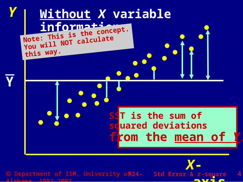
Without X variable information:

SST is the sum of squared deviationsfrom the mean of Y.

Y

Note: This is the concept.

You will NOT calculate

this way.


Y^Using X variable information:Y

X-axis

SSE is the sum of squared deviations from the regression line.

Note: This is the concept.

You will NOT calculate

this way.

Each deviationis a “residual”.


Calculations

SST = (n–1)sy2

SSE

SSR =

Total Variation:

Unaccounted forby regression:

Accounted forby regression:

e 2i=

SST - SSE

3=


Weight vs. Height example:

SSE = 868.06

SST = 4858.00

SSR =

See file M22 &

file M23; or

use computer

output!

See file M22 &

file M23; or

use computer

output!

Example 1, continued


n - 2

e 2 i

Mean Square Error (MSE)

MSE =



Mean Square Error (MSE)

SSE n - 2MSE =

Standard Error of Estimation:Standard Error of Estimation:

MSE = 289.3 = 17.0 lb.

Estimate of “Std. Dev. around the fitted line.”

=

=



r 2 = the “r-square” value r 2 = the “r-square” value

“is the fraction of the total variation of Y accounted for by using regression.”

variation of Y “accounted for”

total variation of Yr

2 =

SSRSSR

SSTSSTrr

22 = =or


0 0 rr22 1.0 1.0

r2 = 0.0 no regression effect;X is NOT useful.

r2 = 1.0 perfect fit to the data;X is USEFUL!


Calculating r2, for Wt vs. Ht

or, have the computer do it for you!

or, have the computer do it for you!

SSR

SSTr2 =

3989.94

4858= = .8213



Equivalently,

r2 = 1.0 - SSE

SST

total variation

“UNaccounted for”


r 2 (correlation)2

= .8213 = (.9063)2

Equivalently,

r2 is also called the “coefficient of determination”“coefficient of determination”r2 is also called the “coefficient of determination”“coefficient of determination”

For the weight-height data:



For the weight-height data:

““82.1% of the total variation 82.1% of the total variation of the of the body weightsbody weights is is accounted for by using accounted for by using

heightheight as a as a predictor variable.”predictor variable.”

r 2

= .8213 Interpretation:


L.O.P.


“ “ % of the total variation % of the total variation of of the the YY-variable-variable is is

accounted for by using accounted for by using thethe XX-variable-variable as a as a predictor variable.”predictor variable.”

r 2

interpretation in general:

L.O.P.


Std. Error of Estimation:

MSE = 289.4 = 17.0 lb.

““The estimated std. dev. ofThe estimated std. dev. ofbody weights body weights around thearound theregression lineregression line is 17.0 pounds.” is 17.0 pounds.”

Interpretation:


L.O.P.


““The estimated std. dev. ofThe estimated std. dev. ofthe the YY-variable-variable around the around theregression line is regression line is unitsunits.”.”

L.O.P.

estimation the regression variation around the regression line

interpretation in general:

Std. Error of


Regression

Error

Total

Source ofVariation

degrees offreedom

Sum ofSquares

MeanSquares

F-Ratio

1*

n – 2**

n - 1

* Number of X-variables used, “k”** n – 1 - k

SSR

SSE

SST

MSR

MSE

SY2

Source DF SS MS =SS

dfF =

MSR

MSE

F

Analysis of Variance Table

Analysis of Variance Table

Regression

Error

Total

Source ofVariation

degrees offreedom

Sum ofSquares

MeanSquares

F-Ratio

1

3

4

3989.94

868.06

4858.00

3989.94

289.35

1214.50

Source DF SS MS =SS

dfF =

MSR

MSE

13.79

Variance of Variance of YY without without XX::Variance of Variance of YY withwith XX::



Y

If we have data for the response variable, but no knowledge of an X-variable, what is the best estimate of the mean of Y?


Y

X

Y

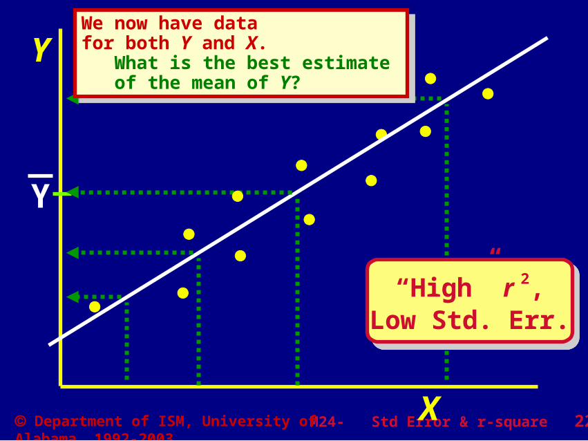
“High” r 2,Low Std. Err.

We now have data for both Y and X. What is the best estimate of the mean of Y?

We now have data for both Y and X. What is the best estimate of the mean of Y?


Y

X

Y

Lower r2,Higher Std. Err.

Lower r 2,Higher Std. Err.

Y

X

Yr 2 = ,

Std. Err. =

Why?

e i2

=SSE =

SST =


RegressionRegression

AnalysisAnalysis

in Minitabin Minitab

RegressionRegression

AnalysisAnalysis

in Minitabin Minitab

More


Example 4 Can the “depth” of lakes Can the “depth” of lakes

be estimated using “surface area”?be estimated using “surface area”?

Lakes in Vilas and Oneida counties in northern Wisconsin from the years 1959-1963.


Regression Analysis

The regression equation isDepth = 28.2 + 0.00726 Area

Predictor Coef StDev T PConstant 28.187 2.443 11.54 0.000Area 0.007262 0.004277 1.70 0.094

S = 17.81 R-Sq = 4.0% R-Sq(adj) = 2.6%

Analysis of VarianceSource DF SS MS F PRegression 1 914.9 914.9 2.88 0.094Error 69 21891.0 317.3Total 70 22805.9

Max. depth in feetsurface area acresData in Mtbwin/data/lake.

Example 4 Estimate depth of lakes using surface area?Estimate depth of lakes using surface area?


Regression Analysis



S = 17.81 R-Sq = 4.0% R-Sq(adj) = 2.6%


Max. depth in feetsurface area acresData in Mtbwin/data/lake.“t” measures how many standard

errors the estimated coefficient is from “zero.”

P-value: a measure of the likelihoodthat the true coefficient is “zero.”



40003000200010000

9080706050403020100

Area

Dep

th

0

2s2s

Example 4 Depth of Lakes (feet) vs. Surface Area (acres)


5448423630

605040302010

0-10-20-30

FITS1

RE

SI1

Example 4 Estimate depth of lakes … Estimate depth of lakes …


How do you determine if theX-variable is a useful predictor?

33See slides 2211

in the previous section.


Regression Analysis



S = 17.81 R-Sq = 4.0% R-Sq(adj) = 2.6%


Max. depth in feetsurface area in acresData in Mtbwin/data/lake.


The P-value for “surface area” IS SMALL (<.10).Conclusion:The “area” coefficient is NOT zero!The “area” coefficient is NOT zero!“Surface area” IS a useful predictor“Surface area” IS a useful predictor of the mean of “depth”. of the mean of “depth”.

Could “area”Could “area”have a truehave a truecoefficient thatcoefficient thatis actually “zero”?is actually “zero”?

Could “area”Could “area”have a truehave a truecoefficient thatcoefficient thatis actually “zero”?is actually “zero”?

Depth of Lakes (feet) vs. Surface Area (acres)

40003000200010000

9080706050403020100

Area

Dep

th

0

2s2s

Where would theline be if theoutlier is removed? ______________.

Example 4


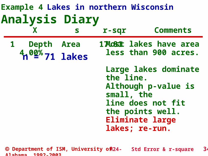
Analysis DiaryStep Y X s r-sqr Comments

1 Depth Area 17.81 4.00% Most lakes have area less than 900 acres. Large lakes dominate the line.Although p-value is small, the line does not fit the points well.Eliminate large lakes; re-run.

Example 4 Lakes in northern Wisconsin

n = 71 lakes


The regression equation isDepth = 25.3 + 0.0226 Area Predictor Coef SE Coef T PConstant 25.325 3.380 7.49 0.000Area 0.02265 0.01454 1.56 0.124 S = 18.00 R-Sq = 3.7% Analysis of Variance Source DF SS MS F PRegression 1 785.8 785.8 2.43 0.124Residual Error 64 20726.1 323.8Total 65 21511.9

Max. depth in feetsurface area in acresData in Mtbwin/data/lake.


n = 66 lakes


700600500400300200100 0

90

80

70

60

50

40

30

20

10

0

Area

De

pth

S = 17.9957 R-Sq = 3.7 % R-Sq(adj) = 2.1 %

Depth = 25.3253 + 0.0226494 Area

Regression Plot


n = 66 lakes

2s2s



1 Depth Area 17.81 4.00% Most lakes have area less than 900 acres. Large lakes dominate.Although p-value is small, the line does not fit the points well.Eliminate large lakes; re-run.

2 Depth Area 18.00 3.70%

n = 71 lakes

Lakes larger than 900 acres in surface area are removed andthe population is redefined. The p-value for “area” is 0.124. “Surface area” is NOT a goodpredictor of lake “depth.”

n = 66 lakes

Example 4 Lakes < 900 acres in northern Wisconsin


How helpful is “engine size” for estimating “mpg”?

Example 5


How helpful is engine size for estimating mpg?

Regression Analysis

The regression equation ismpg_city = 29.3 - 0.0480 displace

113 cases used 4 cases contain missing valuesPredictor Coef StDev T P

Constant 29.2651 0.7076 41.36 0.000displace 0.047967 0.004154 -11.55 0.000

S = 2.880 R-Sq = 54.6% R-Sq(adj) = 54.2%


displacement in cubic in.mpg_city in ??? Data in Car89 Data

Example 5


How helpful is engine size for estimating mpg?Regression Analysis

The regression equation ismpg_city = 29.3 - 0.0480 displace

113 cases used 4 cases contain missing valuesPredictor Coef StDev T P

Constant 29.2651 0.7076 41.36 0.000displace 0.047967 0.004154 -11.55 0.000

S = 2.880 R-Sq = 54.6% R-Sq(adj) = 54.2%


displacement in cubic in.mpg_city in ??? Data in Car89 Data

Example 5

The P-value for “displacement” IS SMALL (<.10).Conclusion:The The “displacement”“displacement” coefficient is NOT zero! coefficient is NOT zero!“Displacement” IS a useful predictor“Displacement” IS a useful predictor of the mean of “mpg_city”. of the mean of “mpg_city”. (But, …(But, …

“t” measures how many standard errors the estimated coefficient is from “zero.”

P-value: a measure of the likelihoodthat the true coefficient is “zero.”


mpg_city vs. displacementmpg_city vs. displacement

35025015050

35

30

25

20

15

displace

mpg

_city

S = 2.88 Is this a good fit? The data pattern appears curved; we can do better!

Example 5


Plot of residuals vs. Y-hatsPlot of residuals vs. Y-hats

27221712

10

5

0

-5

-10

FITS1

RE

SI1

S = 2.88

mpg_city vs. displacementmpg_city vs. displacementExample 5

Apply a transformationin the next section.



1 mpg displac 2.880 54.6%

Slope of “displacement” in not zero; but plot indicates a curvedpattern.Transform a variable and re-run.

Example 5 “mpg_city” versus engine “displacement”

2 to be done in next section.


Which variable is a better predictor of the rating of professional football quarterbacks, percent of touchdown passes or percent of interceptions?

Page 626, Problem 15.23

Example 6


Rating TD% Inter% 96.8 5.6 2.6 92.3 5.1 2.6 87.1 5.4 3.2 86.4 5.0 3.0 85.4 4.0 2.4 84.4 5.0 3.7 83.4 5.2 3.7

Problem 15.23, Page 626

Quarterback Steve Young Joe Montana Brett Favre Dan Marino Mark Brunnell Jim Kelly Roger Staubach

Example 6


Regression Analysis: Rating versus TD%

The regression equation isRating = 65.2 + 4.52 TD%

Predictor Coeff SE Coef T PConstant 65.18 18.90 3.45 0.018TD% 4.520 3.731 1.21 0.280

S = 4.655 R-Sq = 22.7% R-Sq(adj) = 7.2%

Analysis of VarianceSource DF SS MS F PRegression 1 31.82 31.82 1.47 0.280Residual Error 5 108.36 21.67Total 6 140.17

Problem 15.23, Page 626Example 6


Regression Analysis: Rating vs. Interception%

The regression equation isRating = 105 - 5.66 Inter%

Predictor Coef SE Coef T PConstant 105.121 9.767 10.76 0.000Inter% -5.663 3.183 -1.78 0.135

S = 4.144 R-Sq = 38.8% R-Sq(adj) = 26.5%




Which X variable is better for predicting the mean of “Rating”?

What criteria should be used?

TD%

Inter%

Std Error R-Square ______ _______

______ _______


Neither is great;Neither is great;look at plots.look at plots.Neither is great;Neither is great;look at plots.look at plots.


3.53.02.5

95

90

85

Inter%

Ra

ting

S = 4.14354 R-Sq = 38.8 % R-Sq(adj) = 26.5 %

Rating = 105.121 - 5.66273 Inter%

Regression Plot

5.55.04.54.0

95

90

85

TD%

Ra

ting

S = 4.65529 R-Sq = 22.7 % R-Sq(adj) = 7.2 %

Rating = 65.1768 + 4.52018 TD%

Regression Plot

TD% Inter%



Regression Analysis: Rating versus TD%, Inter%

The regression equation isRating = 75.5 + 7.23 TD% - 7.93 Inter%

Predictor Coef SE Coef T PConstant 75.545 7.632 9.90 0.001TD% 7.226 1.543 4.68 0.009Inter% -7.929 1.479 -5.36 0.006

S = 1.819 R-Sq = 90.6% R-Sq(adj) = 85.8%


This is a “multiple regression”Problem 15.23, Page 626Example 7


Which X variable is better for predicting the mean of “Rating”?

TD%

Inter%

Std Error R-Square _______ ________

_______ ________

TD% & Inter% _______ ________

Together, the two variables predict much better than either one individually.



Rating = 75.5 + 7.23 TD% - 7.93 Inter%

Std Error = 1.8190, R-Square = 90.6%

Prediction model for QB Ratings

Notes:Model is based on only n = 7 quarterbacks who played over a 30 year period.


Final Model:


NFL Quarterback Ratings for 2002 season.

NFL Quarterback Ratings.MTW

D:\Edd\Edd\Classes\ST260\data sets

http://espn.go.com/nfl/statistics/glossary.htmlSource:

12

12

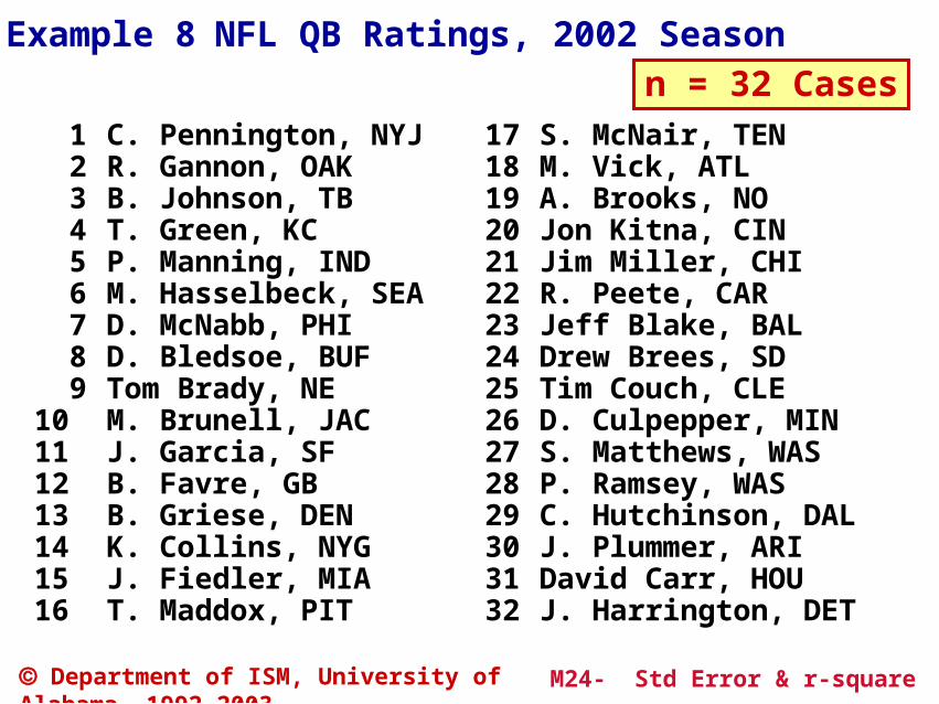
NFL QB Ratings, 2002 SeasonExample 8


C. Pennington, NYJR. Gannon, OAKB. Johnson, TBT. Green, KCP. Manning, INDM. Hasselbeck, SEAD. McNabb, PHID. Bledsoe, BUFTom Brady, NEM. Brunell, JACJ. Garcia, SFB. Favre, GBB. Griese, DENK. Collins, NYGJ. Fiedler, MIAT. Maddox, PIT

S. McNair, TENM. Vick, ATLA. Brooks, NOJon Kitna, CINJim Miller, CHIR. Peete, CARJeff Blake, BALDrew Brees, SDTim Couch, CLED. Culpepper, MINS. Matthews, WASP. Ramsey, WASC. Hutchinson, DALJ. Plummer, ARIDavid Carr, HOUJ. Harrington, DET

1 2 3 4 5 6 7 8 910111213141516

17181920212223242526272829303132


n = 32 Cases


COM CompletionsATT AttemptsCOM% Percentage of completed passesYDS Total YardsYPA Yards per attemptLNG Longest pass playTD Touchdown passesTD% Touchdown percentage TD passes / pass attemptsINT Interceptions thrownINT% Interception percentage Interceptions / pass attemptsSK SacksSYD Sacked yards lostRAT Passer (QB) Rating

Variables MeasuredVariables MeasuredNFL QB Ratings, 2002 SeasonExample 8

k = 12 X-variables


Analysis of Variance Source DF SS MS F PRegression 12 2895.52 241.29 12347.02 0.000Residual Error 19 0.37 0.02Total 31 2895.89

The regression equation isQB Rating = 0.30 - 0.0170 COM + 0.00266 ATT + 0.920 COM% + 0.00123 YDS + 3.59 YPA + 0.00342 LNG - 0.0236 TD + 3.41 TD% - 0.0233 INT - 4.09 INT% - 0.00699 SK + 0.00181 SYD


Minitab output

What is the R-Square?

How many X-variables? How many cases?


10090807060

0.2

0.1

0.0

-0.1

-0.2

Fitted Value

Res

idu

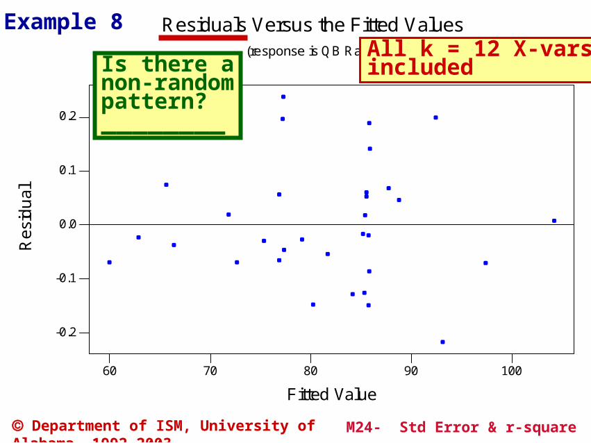
alResiduals Versus the Fitted Values

(response is QB Ratin)

Example 8 All k = 12 X-vars. includedIs there a

non-randompattern?________

Predictor Coef SE Coef T PConstant 0.302 1.641 0.18 0.856COM -0.016982 0.007611 -2.23 0.038ATT 0.002657 0.003952 0.67 0.509COM% 0.91976 0.03536 26.01 0.000YDS 0.0012311 0.0005133 2.40 0.027YPA 3.5921 0.2369 15.16 0.000LNG 0.003418 0.002331 1.47 0.159TD -0.02358 0.04552 -0.52 0.610TD% 3.4065 0.2086 16.33 0.000INT -0.02333 0.04706 -0.50 0.626INT% -4.0876 0.2165 -18.88 0.000SK -0.006990 0.007671 -0.91 0.374SYD 0.001806 0.001335 1.35 0.192S = 0.1398 R-Sq = 100.0% R-Sq(adj) = 100.0%


Minitab output All k = 12 X-vars. included

Do we need all 12 variables? Which is least useful?



Comments:

1. Always leave the constant termconstant term in the model.

2.2. Never delete more than ONENever delete more than ONE X-variable per run;re-run the regression at each step, each time deleing only one variable.

3. A “backward eliminationbackward elimination” can speed-up the process.

4. At the last step, re-assess your modelre-assess your model bychecking the residual plots again.



Backward Elimination ProcessBackward Elimination ProcessStep Step Var. Out?Var. Out? t p s R t p s R2 2 Action Action

1 INT -.023 .626 .14099.99 2 ATT .48 .639 .137 99.99

DeleteDelete

Re-run regression with one less variable;determine the least useful of the remainingvariables. (Look for the largest P-value).

Re-run regression with one less variable;determine the least useful of the remainingvariables. (Look for the largest P-value).



Backward Elimination ProcessBackward Elimination ProcessStep Step Var. Out?Var. Out? t p s R t p s R2 2 Action Action

1 INT -.023 .626 .14099.99 2 ATT .48 .639 .137 99.99

6 LNG 2.04 .053 .136 99.98

3 TD -.43 .674 .135 99.99 4 SK -.87 .394 .132 99.99 5 SYD 1.61 .121 .131 99.99

10 INT% -8.09 .000 2.030 96.02 9 YPA 66.01 .000 .162 99.98 8 COM -1.36 .186 .160 99.98 7 YDS 2.65 .014 .144 99.98

13 Constant 9.67 0.00012 COM% 8.63 .000 5.260 73.0011 TD% 5.80 .000 3.640 86.71

DeleteDelete


The regression equation isQB Rating = 2.13 + 0.833 COM% + 4.20 YPA + 3.29 TD% - 4.19 INT%

Predictor Coef SE Coef T PConstant 2.1295 0.4179 5.10 0.000COM% .832514 0.008313 100.14 0.000YPA 4.19967 0.06362 66.01 0.000TD% 3.29368 0.04121 79.92 0.000INT% -4.18577 0.03856 -108.56 0.000

S = 0.1622 R-Sq = 100.0%

Analysis of Variance

Source DF SS MS F PRegression 4 2895.18 23.79 27500.39 0.000Residual Error 27 0.71 0.03Total 31 2895.89

Example 8 Result after dropping 8 X-variables:


10090807060

0.3

0.2

0.1

0.0

-0.1

-0.2

-0.3

Fitted Value

Res

idu

alResiduals Versus the Fitted Values

(response is QB Ratin) k = 4 X-vars. included.

Is there anon-randompattern?

NoNo


2.1295 0.8325 4.1997 3.2937-4.1858

ConstantCompletions per AttemptYards per AttemptTD per AttemptInterception per Attempt

RegressionEstimates

Final Prediction Model Final Prediction Model NFL QB Ratings, 2002NFL QB Ratings, 2002

Example 8

Std Error = 0.160, R-Square = 99.98%

Variables

Result using 4 X-variables:


Step 1: Complete passes divided by pass attempts. Subtract 0.3, then divide by 0.2

Step 2: Passing yards divided by pass attempts. Subtract 3, then divide by 4.

Step 3: Touchdown passes divided by pass attempts, then divide by .05.

Step 4: Start with .095, and subtract interceptions divided by attempts. Divide the difference by .04.

The sum of each step cannot be greater than 2.375or less than zero.Add the sum of the Steps 1 through 4,multiply by 100 and divide by 6.

Actual Rating Formula:NFL QB Ratings, 2002 SeasonExample 8


RegressionEstimates

2.1295 0.8325 4.1997 3.2937-4.1858

2.0833 0.8333 4.1667 3.3333-4.1667

Actual Values*

* Ignoring limits for each part.


ConstantCOMP%YPATD%INT%

Comparison of true to estimatesComparison of true to estimates






















































































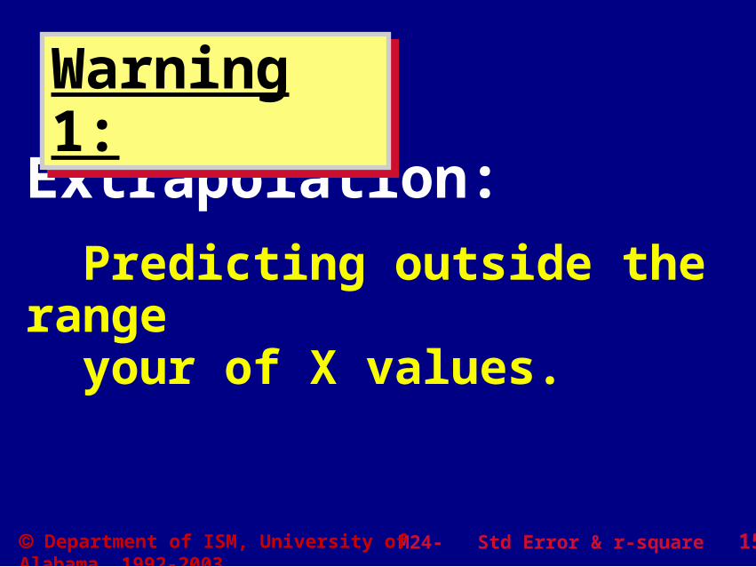
Extrapolation:

Predicting outside the range your of X values.

Warning 1: Warning 1:


A strong relationship between Y and X does not imply “cause and effect.”




Be sure your model looksreasonable!

Remember to DTDP.


Summarizing the relationship between X and Y

Estimating the mean level of Y for a given value of X

Predicting future values of Y for given values of X

Uses of the regression line:

M24- Std Error & r-square 1 Department of ISM, University of Alabama, 1992-2003 Lesson Objectives Understand how to calculate and interpret the “r-square”

Documents

r square slide

m24 std error rsquare

rsquare value

calculating r

department of ism

university of alabama

ssr sst r

total variation of y