Lyman-Alpha-Emitting Galaxies at z = 2.1 in ECDF-S: Building Blocks of Typical Present-day Galaxies?

Astrophysical Journal, in press

Lyα-Emitting Galaxies at z = 2.1 in ECDF-S: Building Blocks of Typical

Present-day Galaxies?1

Lucia Guaita2, Eric Gawiser3, Nelson Padilla2, Harold Francke2, Nicholas A. Bond3,

Caryl Gronwall4, Robin Ciardullo4, John J. Feldmeier5, Shawn Sinawa4,

Guillermo A. Blanc6, Shanil Virani7

[email protected]

ABSTRACT

We discovered a sample of 250 Lyα emitting (LAE) galaxies at z ' 2.1 in an ultra-

deep 3727A narrow-band MUSYC image of the Extended Chandra Deep Field-South.

LAEs were selected to have rest-frame equivalent widths (EW) > 20 A and emission

line fluxes FLyα > 2.0× 10−17 erg cm−2 s−1, after carefully subtracting the continuum

contributions from narrow-band photometry. The median emission line flux of our

sample is FLyα = 4.2× 10−17 erg cm−2 s−1, corresponding to a median Lyα luminosity

LLyα = 1.3 × 1042 erg s−1 at z ' 2.1. At this flux our sample is ≥ 90 % complete.

Approximately 4% of the original NB-selected candidates were detected in X-rays by

Chandra, and 7% were detected in the rest-frame far-UV by GALEX; these objects were

eliminated to minimize contamination by AGN and low-redshift galaxies. At LLyα ≥1.3 × 1042 erg s−1, the equivalent width distribution is unbiased and is represented

by an exponential with scale-length 83 ±10 A. Above this same luminosity threshold,

we find a number density of 1.5 ± 0.5 × 10−3 Mpc−3. Neither the number density of

LAEs nor the scale-length of their EW distribution show significant evolution from

z ' 3 to z ' 2. We used the rest-frame UV luminosity to estimate a median star

formation rate of 4 M yr−1. The median rest-frame UV slope, parametrized by the

color B−R, is that typical of dust-free, 0.5-1 Gyr old or moderately dusty, 300-500 Myr

old population. Approximately 30% of our sample is consistent with being very young

(age < 100 Myr) galaxies without dust. Approximately 40% of the sample occupies the

2Departmento de Astronomia y Astrofisica, Universidad Catolica de Chile, Santiago, Chile

3Department of Physics and Astronomy, Rutgers, The State University of New Jersey, Piscataway, NJ 08854

4Department of Astronomy&Astrophysics Penn State University, State College, PA 16802

5Department of Physics and Astronomy, Youngstown State University, Ohio 44555-2001

6Department of Astronomy, University of Texas at Austin, Austin, TX 78712

7Department of Astronomy, Yale University, New Haven, CT 06520-8101

arX

iv:0

910.

2244

v2 [

astr

o-ph

.CO

] 9

Mar

201

0

– 2 –

z ∼ 2 star-forming galaxy locus in the UV R two color diagram, but the true percentage

could be significantly higher taking into account photometric errors. Clustering analysis

reveals that LAEs at z ' 2.1 have r0 = 4.8 ± 0.9 Mpc, corresponding to a bias factor

b = 1.8± 0.3. This implies that z ' 2.1 LAEs reside in dark matter halos with median

masses log(M/M) = 11.5+0.4−0.5, which are among of the lowest-mass halos yet probed

at this redshift. We used the Sheth & Tormen conditional mass function to study the

descendants of these LAEs and found that their typical present-day descendants are

local galaxies with L∗ properties, like the Milky Way.

Subject headings: galaxies: photometry – surveys – galaxies: high-redshift – galaxies:

star formation

1. Introduction

The search for high-redshift star-forming galaxies advanced rapidly with the introduction of

the Lyman Break Galaxies (LBG) technique (Guhathakurta et al. 1990, Steidel & Hamilton 1992,

Steidel et al. 1999) that takes advantage of the lack of flux at wavelengths shorter than the Lyman

break at 912 A rest frame due to absorption of ionizing photons by neutral hydrogen, located

in stellar atmospheres, in the interstellar medium (ISM), and in the intergalactic medium (IGM)

between galaxies. At z = 3 the break is located in the observed U band and at higher redshift it

moves into optical and infrared bands. This has allowed an exploration of star-forming galaxies at

redshifts 3 ≤ z ≤ 8 via imaging from ground and space (e.g. Steidel et al. 2003, Bouwens et al. 2006,

Ouchi et al. 2008) and spectroscopy on 8–10 meter telescopes (e.g. Shapley et al. 2001, Shapley

et al. 2003). A significant fraction of high redshift LBGs show the Lyα line in emission (Shapley

et al. 2001). This emission offers additional information about the process of star formation inside

these galaxies and radiative transfer in their ISM.

Looking for galaxies with Lyα in emission has become an important photometric technique that

permits us to find faint (R ∼ 27) star-forming galaxies at high redshift. This technique consists of

comparing the flux density measured in a narrow-band filter, revealing observed-frame Lyα emission

to that found in the broad-band filters, representing the continuum. Thanks to the intensity of

this emission line, the resulting Lyα emitting (LAE) galaxies provide a special population of high

redshift galaxies. The properties of LAEs have been extensively studied at z ≥ 3 (e.g. Ouchi et al.

2005, Venemans et al. 2005, Gawiser et al. 2006b, Gronwall et al. 2007, Nilsson et al. 2007). LAE

samples are composed primarily of galaxies fainter in the continuum than LBGs; Lyα Emitting

galaxies therefore probe the lowest bolometric luminosities at high redshift.

1Based on observations obtained at Cerro Tololo Inter-American Observatory, a division of the National Optical

Astronomy Observatory, which is operated by the Association of Universities for Research in Astronomy, Inc., under

cooperative agreement with the National Science Foundation.

– 3 –

Theoretical models, that include radiative transfer inside star-forming galaxies (Verhamme

et al. 2006, Schaerer & Verhamme 2008, Verhamme et al. 2008, Atek et al. 2009), were also developed

to understand how Lyα photons form in HII regions and then escape the galaxy, depending on

resonant scattering by neutral hydrogen, dust absorption and velocity dispersion in the interstellar

medium. The amount of dust and the interstellar medium geometry can affect the escape of Lyα

photons and hence the shape of the line. Clumpy media could permit Lyα photons to escape, even

if the galaxy is not dust-free (Neufeld 1991, Finkelstein et al. 2008, Finkelstein et al. 2009).

Spectral Energy Distribution (SED) fitting of the stacked multi-wavelength photometry of

z ' 3 LAEs (Gawiser et al. 2007, Lai et al. 2008) shows they are a young (median starburst age

of ∼ 20 Myr), low stellar mass (M∼ 109 M), modest SFR (median SFR ∼ 2 M yr−1), low dust

(AV ≤0.2) population of galaxies in an active phase of star formation. SEDs have also shown older

population best fits for subsamples of LAEs at z > 3 (Pirzkal et al. 2007, Ono et al. 2009, Nilsson

et al. 2009). SED fitting of individual galaxies showed older ages, higher stellar mass and more

dust for continuum-bright LAEs drawn from LBG samples (Shapley et al. 2001, Tapken et al. 2007,

Pentericci et al. 2009). Stiavelli et al. (2001) had also shown redder colors for some LAEs at z ' 2.4.

Recently Nilsson et al. 2009 presented the first results of observations of LAEs at z ' 2.3, inferring

evolution in the properties from z ∼ 3 to z ∼ 2, with more diversity in photometric properties at

z ' 2.3.

Clustering analysis of LAEs showed z ≥ 4 LAE bias factors (Kovac et al. 2007, Ouchi et al.

2004) expected for progenitors of massive elliptical galaxies in the local Universe, while z ' 3.1

LAEs could be progenitors of L∗ galaxies (Gawiser et al. 2007). Semi-analytical simulations were

also able to reproduce these results (Orsi et al. 2008). Lower redshift observations, including

clustering, will reveal evolution from high to low redshift. For this reason we were motivated to

study LAE samples at redshift around 2. This will trace the star formation properties of this type

of galaxy at the epoch of the peak of cosmic star formation density (Madau et al. 1998, Giavalisco

et al. 2004). It also promises to reveal z ∼ 0 descendants of LAEs at z ' 2.1.

In this paper we describe the results from ultra-deep 3727 A narrow-band MUSYC (MUlti-

walengthSurvey Yale Chile, Gawiser et al. 2006a) imaging of the 998 arcmin2 Extended Chandra

Deep Field-South. In sections 2 and 3 we present the observations and the data reduction. In

Section 4 we summarize the selection of the LAE sample and estimate the possible contaminants.

We present the properties of the LAE sample in Section 5: number density, star formation rate,

colors and clustering. In Section 6 we discuss the results and derive conclusions.

We assume a ΛCDM cosmology consistent with WMAP 5-year results (Dunkley et al. 2009,

their table 2), adopting the mean parameters Ωm = 0.26, ΩΛ = 0.74, H0 = 70 km sec−1 Mpc−1,

σ8 = 0.8.

– 4 –

2. Observations

Our observations of the Extended Chandra Deep Field-South (ECDF-S) were carried out at

the CTIO Blanco 4m telescope, using the MOSAIC II CCD camera (eight 2048 × 4096 CCDs, each

with two amplifiers). We took advantage of public broad-band UBV RI images of ECDF-S taken

with WFI at the ESO 2.2m telescope, processed by the Garching-Bonn Deep Survey (GaBODS,

Hildebrandt et al. 2006), and reprojected to match the MUSYC BV R image (Table 1).2 We use

NB3727 to detect the Lyα emission line flux and a weighted combination of U and B to measure

the continuum flux density. Fig. 1 shows the transmission curves of these filters.

We used the narrow-band filter with response centered at 3727 A (FWHM=50 A), originally

designed to detect the [OII] emission line, corresponding to the Lyα emission line wavelength at

z = 2.07 ± 0.02. Our field was imaged during 2007, December 3 − 13, using hour-long exposures

to avoid the read-out noise limit (see Table 2). The total exposure time was about 36 hours and

the median seeing of the run was 1.4”. The raw images cover a field of view of 36×36 arcmin2, the

ECDF-S (central coordinates Right Ascension = 3h32m29s, angular Declination = -27o48′47”).

3. Data Reduction

The NB3727 narrow-band data were reduced using the IRAF mscred package designed to

process MOSAIC frames. We followed the NDWFS (NOAO Deep Wide-Field Survey) cookbook 3

as modified by Gawiser et al. (2006a) plus a few additional steps described below. The principal

steps in the reduction process were:

i) Creating and applying an improved Bad Pixel Mask (BPM). To better represent the distribution

of bad pixels and columns than the default BPM, we combined together all the twilight flats and all

the object frames of the run in the NB3727 filter. We used the sflatcombine task, which takes into

account the difference in signal levels (exposure times), to make a median combination of the input

frames. The features in the combined frame represent bad pixels and columns that are present in

all the frame files. Applying the ccdproc task to all the raw bias, sky flat and object frames, we

replaced the updated version of BPM regions through linear interpolation between good pixels;

ii) Improving the World Coordinate System (WCS) information provided in the header of the raw

object frames, using interactively the msccmatch task. To estimate the astrometric correction,

we built a list of point (stellarity parameter > 0.8) sources from the MUSYC ECDF-S catalog 4,

detected in a deep composition of B, V , R bands. The sources are uniformly distributed in the

field, not saturated, but bright enough (11 < B < 21, 10 < R < 18) to be seen in the narrow-band

image;

2These images will be available as part of the MUSYC public data release, labelled v2.

3http://www.noao.edu/noao/noaodeep/ReductionOpt/frames.html

4http://www.astro.yale.edu/MUSYC/

– 5 –

iii) Removing cosmic rays (CRs), particularly important given the single frame exposure time of

one hour. We used LACOSMIC software package (van Dokkum 2001 5) with 4 iterations. Cosmic

ray pixels (image features with sharp edges) were replaced by the median of the surrounding good

pixels. We chose a contrast limit between CR and underlying object equal to 5, as required for a

conservative discrimination between bright stars and cosmic rays and a CR detection limit designed

for HST space images. These CR pixels are added to the BPM;

iv) Transforming the MOSAIC frames into tangent plane projected images with mscimage. To be

able to stack all the images of the run into one deep image, we used the MUSYC BV R image as a

reference to define the tangent point, orientation and the pixel scale of 0.267′′ pixel−1;

v) Matching signal levels using mscimatch. We defined a scaling between each exposure frame,

comparing the intensities of a sample of point sources from the MUSYC BV R catalog. We sep-

arated all the hour-long NB3727 images into two groups of ∼18 hours each that we call the first

(1H) and second (2H) half of the run. We later used the two halves of the run to search for spurious

sources revealed by significant flux variations between the two halves;

vi) Stacking of all the first and second half images, following the point-source-optimized weighting

procedure developed by Gawiser et al. (2006a). In Table 3 we show the properties of all the images

of the run. As the final step of the image reduction, we applied mscimatch to the two halves to

scale them in intensity and then performed a weighted stack of the two halves to create the final

NB3727 image of the full run. The overall seeing of the final image is 1.4′′;

vii) Estimating and subtracting the sky background using the Source Extractor program (SExtrac-

tor, Bertin & Arnouts 1996). The sky background was estimated as the average of the background

counts in boxes of 64 × 64 pixels and then the average was median-filtered smoothed across six 64

× 64 pixel boxes;

viii) Shifting and trimming our final stacked image to have the same size and areal coverage as our

reference MUSYC BV R and hence the other MUSYC broad-band images, covering 31.6’ × 31.6’

at 0.267 arcsec/pixel scale (Gawiser et al. 2006a);

ix) Normalized to effective exposure time of one second and added photometric calibration for the

final NB3727 image and both halves. As the photometric calibration was determined using Galactic

stars, for extragalactic studies we subtracted off the factor Aλ = 0.05 mags, as appropriate for the

near-UV wavelength range and E(B-V) = 0.01 at this location, to account for extinction by dust

in the Milky Way (Schlegel et al. 1998). Photometric calibration of NB3727 via Landolt standard

and spectrophotometric standard stars proved challenging, so we adjusted the nominal photomet-

ric calibration by 0.35 magnitude to set the median UB−NB3727 color (defined in §4) to zero in

AUTO photometry. This causes star colors to match those predicted by Pickles (1998) templates

to within 0.1 magnitudes.

5http://www.astro.yale.edu/dokkum/lacosmic

– 6 –

4. SAMPLE SELECTION

We extracted sources following the method described in Gawiser et al. (2006a). We used SEx-

tractor to detect and extract sources from the final NB3727 image. We filtered by the approximate

PSF (a 9×9 pixel Gaussian grid with FWHM 5 pixels) and required a minimum of one pixel above

the chosen threshold of 0.8 sigma. We optimized this detection threshold to detect the highest

number of sources while avoiding a large percentage of spurious ones. We estimated the number of

spurious objects, assuming symmetrical background fluctuations, by running SE on the “negative”

of the narrow-band image (narrow-band image multiplied by “-1”) and counting the number of

negative detections as a function of our parameters.

We ran SExtractor in dual mode with the NB3727 narrow band as the detection image and

each of the MUSYC broad bands (UBV RIzJHK plus U38) and the 1H and 2H stacks as the

measurement images. For each of 19455 sources in the NB3727 catalog, this measured their cor-

responding fluxes in the other bands. We used the corrected-aperture method from Gawiser et al.

2006a to convert optimized-aperture to total APCORR fluxes. Most objects in our NB3727 de-

tected catalog have relatively low signal-to-noise. By comparing with the higher S/N broad-band

images, we found an 0.1” rms offset between the narrow-band detection image centroid and the

better-determined broad-band centroid, implying a consequent 13% underestimate of broad-band

flux of our catalog objects. Bright sources do not exhibit these centroiding errors, so it is not a

problem of astrometry. To compensate this loss, we increased the broad-band APCORR fluxes by

this amount. The signal-to-noise for point sources in the NB3727 stacked image was optimized

using an aperture diameter of 1.4′′ which contains 40% of the signal for point sources. In the case

of broad-band images, the optimal aperture had 1.2” diameter, which contains 41% of U and 43%

of B point source flux.

LAE candidates were selected with the following criteria:

1. Narrow-band detection at 5σ significance. We chose objects with magnitudes brighter than the

typical 5σ NB3727 detection limit of magnitude 25.1, corresponding to Lyα line fluxes, FLyα >

2.0×10−17 erg sec−1 cm−2 and luminosities, LLyα > 6.4×1041 erg sec−1, after carefully subtracting

the continuum contributions from narrow-band photometry (see Appendix for details, equations

(A1)-(A10)). 16,872 objects of our catalog satisfy this “global” signal-to-noise criterion.

2. Local signal-to-noise > 5. Our analysis of detections in the negative image indicated that

the global S/N criterion would still leave 33 fake sources. These fake sources are concentrated in

the region of the amplifier with the highest readout noise. Even though SExtractor uses a semi-

local measurement of the background rms as a detection threshold, we found that applying an

additional cut of the ratio between the aperture flux and the photometric error on it bigger than

5, faper/σfaper > 5, eliminated all but 7 of the detections in the negative image. Implementing

this criterion, most of the excluded objects are located in the region of that noisiest amplifier,

that would otherwise have been classified as LAEs. 15,882 objects satisfy the first and this second

criteria.

3. Narrow-band excess corresponding to EW> 20A . We defined a color UB−NB3727 as the

– 7 –

difference in magnitudes between the UB and NB3727 flux densities (see Appendix, equations

(A12),(A13),(A14)), where UB refers to the linear combination of U and B flux densities, fUB =

0.8fU +0.2fB, motivated by the central wavelengths of the filters. A positive value of UB−NB3727

indicates an excess in the narrow-band flux density. In order to obtain an Equivalent Width

(EW) rest-frame cut of EW >20 A (Gronwall et al. 2007, §5.2 of this paper), we required UB-

NB3727>0.73. (Fig. 2). This generated an initial list of 367 LAE candidates.

4. 1σ significance of the narrow-band excess versus a pure continuum spectrum. We required

fNB3727 − fUB >√σ2(fNB3727) + σ2(fUB) (1)

to avoid contamination by continuum-only objects whose narrow-band photometry fluctuated up-

wards or continuum photometry fluctuated downwards due to Poisson statistics. While this only

requires the presence of a narrow-band flux density excess at 1σ significance, combined with the

requirement of UB−NB3727> 0.73, it appears to avoid most such contaminants, at the cost of

some incompleteness as discussed further in §4.1. It also has the benefit of eliminating a number

of objects with poor photometry from the sample by virtue of their larger photometric uncertain-

ties. Most objects that passed the previous criteria, but were eliminated by this one, are faint (AB

magnitude NB3727∼24.0) and extended (NB3727 half light radius >1.4′′). They consist of multiple

objects in the deepest BV R image that are blended by the larger NB3727 PSF into single faint ob-

jects centered between the BV R object positions. In this case, aperture photometry at the NB3727

centroid underestimates the continuum flux, leading to a false narrow-band excesses. Because the

APCORR pipeline includes an extended object correction and flux uncertainty increase based upon

the half light radius, these objects have large enough uncertainty in their narrow-band flux excess

to be eliminated by this criterion. 48 objects are excluded after including this requirement, leaving

319 objects.

5. Lack of variation in narrow-band flux between first and second half stacks. We exclude four

objects for which

|f1H − f2H | > 3√σ2

1H + σ22H (2)

where f1H and f2H correspond to an object’s flux density in the stacked NB3727 images of the first

and second halves of the run and σ represents the uncertainty on each.

As the two halves of the run are separated by only a few nights, even AGN are unlikely to show

measurable variability on these time-scales. Hence this is primarily a method for eliminating

objects whose narrow-band excess appears spurious, perhaps coming from a single image due to an

incompletely subtracted cosmic ray or from a contiguous set of images due to a systematic flaw in

bias subtraction or flat-fielding. After this correction, 315 objects remain.

6. No saturated pixels. We exclude objects satisfying the above criteria that had a maximum

SExtractor flag≥ 4, implying either uncorrected bad pixels in o2 (4 objects), detections too close

to the image border to trust (2 objects), or continuum magnitude bright enough to saturate in at

least one band (0 objects at this stage) leaving 309 objects.

7. Not consistent with cross-talk contamination from a bright star. The electronic coupling of

adjacent amplifiers on MOSAIC II is a serious obstacle for narrow-band excess searches, as a

– 8 –

number of the couplings produce echoes that have the same dithering pattern as real objects. A

careful analysis of bright star positions versus locations of narrow-band excess sources determined

the cross-talk offset to be ±2100±10 pixels in declination and 0±10 pixels in right ascension. These

offsets were used to generate a cross-talk mask that excluded 15 of our original LAE candidates

with only 2 such matches expected by chance. Visual inspection and analysis of the EW of these

objects implies that the vast majority were indeed spurious, so this masking should cause negligible

incompleteness in our sample. After the exclusion of these 15 cross-talks, 294 objects remain in the

list.

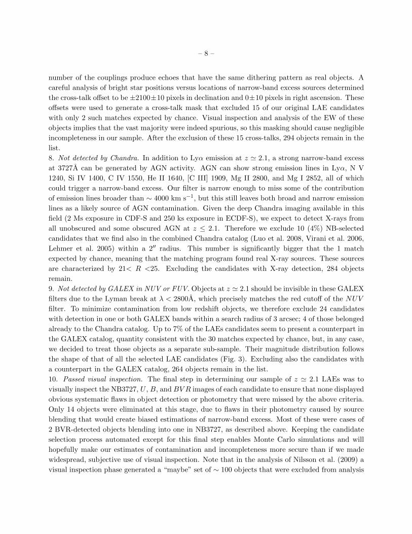
8. Not detected by Chandra. In addition to Lyα emission at z ' 2.1, a strong narrow-band excess

at 3727A can be generated by AGN activity. AGN can show strong emission lines in Lyα, N V

1240, Si IV 1400, C IV 1550, He II 1640, [C III] 1909, Mg II 2800, and Mg I 2852, all of which

could trigger a narrow-band excess. Our filter is narrow enough to miss some of the contribution

of emission lines broader than ∼ 4000 km s−1, but this still leaves both broad and narrow emission

lines as a likely source of AGN contamination. Given the deep Chandra imaging available in this

field (2 Ms exposure in CDF-S and 250 ks exposure in ECDF-S), we expect to detect X-rays from

all unobscured and some obscured AGN at z ≤ 2.1. Therefore we exclude 10 (4%) NB-selected

candidates that we find also in the combined Chandra catalog (Luo et al. 2008, Virani et al. 2006,

Lehmer et al. 2005) within a 2′′ radius. This number is significantly bigger that the 1 match

expected by chance, meaning that the matching program found real X-ray sources. These sources

are characterized by 21< R <25. Excluding the candidates with X-ray detection, 284 objects

remain.

9. Not detected by GALEX in NUV or FUV. Objects at z ' 2.1 should be invisible in these GALEX

filters due to the Lyman break at λ < 2800A, which precisely matches the red cutoff of the NUV

filter. To minimize contamination from low redshift objects, we therefore exclude 24 candidates

with detection in one or both GALEX bands within a search radius of 3 arcsec; 4 of those belonged

already to the Chandra catalog. Up to 7% of the LAEs candidates seem to present a counterpart in

the GALEX catalog, quantity consistent with the 30 matches expected by chance, but, in any case,

we decided to treat those objects as a separate sub-sample. Their magnitude distribution follows

the shape of that of all the selected LAE candidates (Fig. 3). Excluding also the candidates with

a counterpart in the GALEX catalog, 264 objects remain in the list.

10. Passed visual inspection. The final step in determining our sample of z ' 2.1 LAEs was to

visually inspect the NB3727, U , B, andBV R images of each candidate to ensure that none displayed

obvious systematic flaws in object detection or photometry that were missed by the above criteria.

Only 14 objects were eliminated at this stage, due to flaws in their photometry caused by source

blending that would create biased estimations of narrow-band excess. Most of these were cases of

2 BVR-detected objects blending into one in NB3727, as described above. Keeping the candidate

selection process automated except for this final step enables Monte Carlo simulations and will

hopefully make our estimates of contamination and incompleteness more secure than if we made

widespread, subjective use of visual inspection. Note that in the analysis of Nilsson et al. (2009) a

visual inspection phase generated a “maybe” set of ∼ 100 objects that were excluded from analysis

– 9 –

despite not presenting obvious flaws; our approach is the opposite, which has significant advantages

for achieving completeness. We will discuss possible sources of contamination in the next section.

Our final sample consists of 250 z ' 2.1 LAEs in 998 arcmin2.

4.1. Contamination Estimates

In our sample analysis we considered four possible remaining sources of contamination:

1. Spurious objects, manifesting as pure NB3727 emitters with zero continuum, which causes signif-

icant fractional uncertainties on the broad-band flux densities. We conducted detailed simulations

of false object detection by using SExtractor to search for objects in the “negative” image defined

above using identical detection parameters. This predicts that our sample of LAEs includes 7 false

objects, all of them with 24<NB3727<25.1, UB-NB3727 > 0.7, UB-NB3727 > 0 at 1σ. An em-

pirical analysis was also performed. Since false objects detected in NB3727 have zero continuum,

photometric errors should push half to positive and half to negative flux densities in our deepest

continuum image, BV R, due to the symmetry of fluctuations. Hence finding 1 LAE with negative

flux density in BV R yields a best estimate of 2 spurious objects. Combining these two approaches

and the following discussion in the Appendix, we estimate contamination by 4+3−2 spurious sources.

We found counterparts in the GEMS 6 HST-ACS V -band images for 90% of our LAEs. Since LAEs

are selected via emission-line excess, no continuum is required, but this analysis does set an upper

limit of 10% for our contamination by spurious objects (which should not have GEMS counter-

parts). Similarly we found a 70% counterpart match rate between z ' 2.1 LAEs and the MUSYC

BV R catalog, which are not as deep as GEMS V -band and therefore place a weaker constraint on

contamination by spurious objects.

2. Continuum only objects that show an NB3727 excess due to photometric noise. We assume that

continuum-only contaminants are in the range 24 < NB3727 < 25.1, as the few brighter candidates

would have good photometry. We fit with a Gaussian curve the distribution of the UB−NB3727

color for the original catalog of objects with 24 < NB3727 < 25.1 (Fig. 2b). As the Gaussian

σ is equal to 0.2, we are selecting objects above 3.5σ using our color cut. Comparing the ratio

between the integrated area at UB−NB3727 > 0.73 and under the Gaussian curve in the range

−0.5 ≤ UB-NB3727 ≤ 0.5, and accounting for uncertainties in the Gaussian fit, we estimate that

5+10−3 contaminants belong to the sample selected via UB−NB3727 > 0.73.

3. Lower redshift emission line galaxies i.e., [O II] emitters. We expect virtually none of these ob-

jects to contaminate our sample, due to their tiny number density at rest-frame EW> 20A (Hogg

et al. 1998) and the small volume available for z'0 objects. Local Universe [OII] emitters would

be several arcsec across, so would stand out clearly in our catalogs. In any case the exclusion of

GALEX detected sources should rule out this contribution.

4. Obscured AGN, which are capable of triggering a narrow-band excess through their narrow

6http://www.mpia-hd.mpg.de/GEMS/gems.htm

– 10 –

emission lines. Since we found 10 AGN as X-ray sources in the Chandra catalog and some of those

may be obscured or Compton thick, and most models predict a roughly equal number of obscured

and unobscured AGN at this redshift (Treister et al. 2004), we set an upper limit on residual AGN

contamination of 10±10 objects. This will be probed via follow-up spectroscopy. Note that heavily

obscured AGN may not show any emission lines at all and therefore would not be found in our

sample; this reinforces confidence in our upper limit. We stacked 66 LAEs in our sample with

coverage in the 2Ms CDFS image (Luo et al. 2009) and found 3σ upper limits for the soft-band

(hard-band) stacked flux of 4×10−18 (2 ×10−17) erg s−1 cm−2, corresponding to a luminosity of

1.3 ×1041 (6.7×1041) erg s−1 at z = 2.1. The observed soft-band implies a 3σ upper limit on the

average SFR of 30 M yr−1 (Ranalli et al. 2003). Compared to our typical rest-UV SFR of 4 Myr−1 this implies that the dust correction must be less than a factor of seven. Because individual

X-ray detections above the 2Ms flux limit of 2×10−17 erg s−1 cm−2 were removed from our LAE

sample in this region, any AGN remaining must have soft-band luminosity below 7×1041 erg s−1. In

the extreme case, 20% of our sample could contain low-luminosity AGN just below this threshold;

this provides a weaker constraint on AGN contamination than those mentioned above.

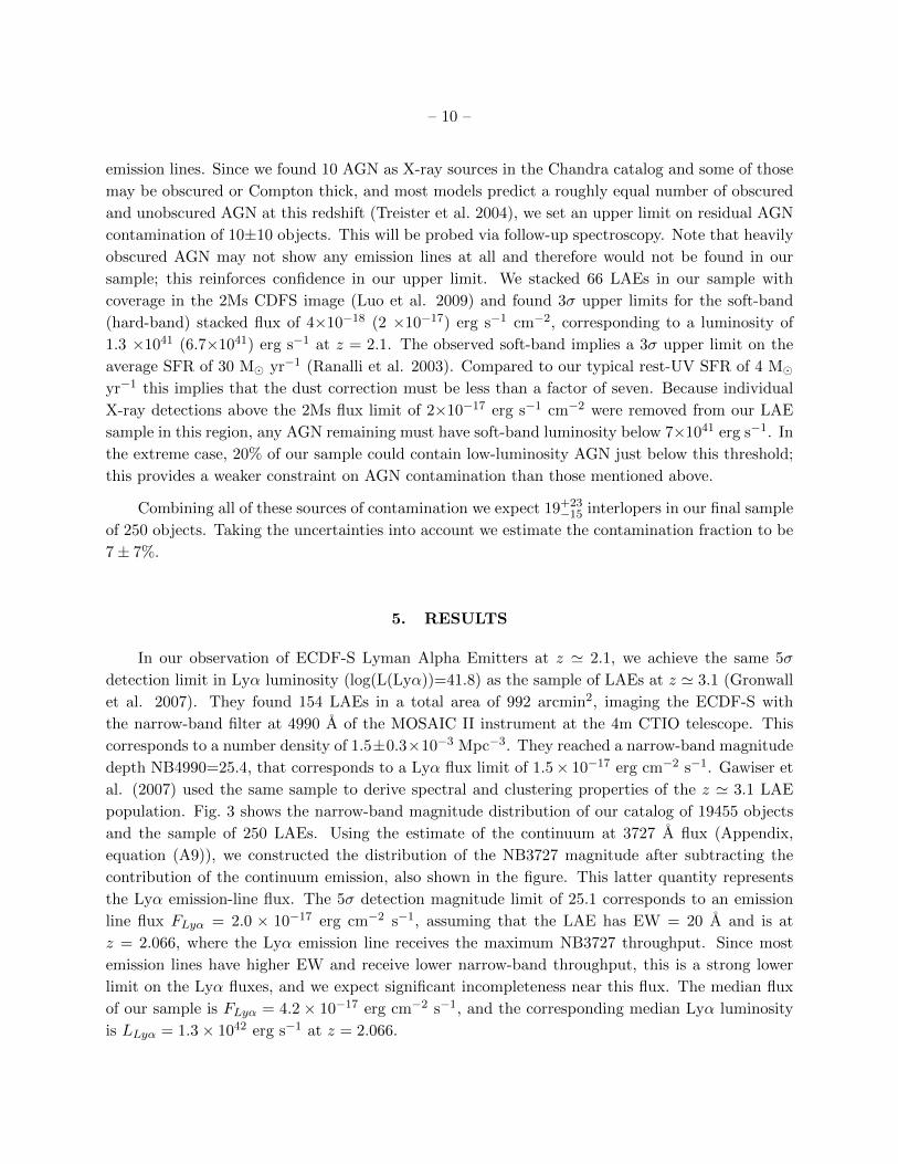
Combining all of these sources of contamination we expect 19+23−15 interlopers in our final sample

of 250 objects. Taking the uncertainties into account we estimate the contamination fraction to be

7± 7%.

5. RESULTS

In our observation of ECDF-S Lyman Alpha Emitters at z ' 2.1, we achieve the same 5σ

detection limit in Lyα luminosity (log(L(Lyα))=41.8) as the sample of LAEs at z ' 3.1 (Gronwall

et al. 2007). They found 154 LAEs in a total area of 992 arcmin2, imaging the ECDF-S with

the narrow-band filter at 4990 A of the MOSAIC II instrument at the 4m CTIO telescope. This

corresponds to a number density of 1.5±0.3×10−3 Mpc−3. They reached a narrow-band magnitude

depth NB4990=25.4, that corresponds to a Lyα flux limit of 1.5× 10−17 erg cm−2 s−1. Gawiser et

al. (2007) used the same sample to derive spectral and clustering properties of the z ' 3.1 LAE

population. Fig. 3 shows the narrow-band magnitude distribution of our catalog of 19455 objects

and the sample of 250 LAEs. Using the estimate of the continuum at 3727 A flux (Appendix,

equation (A9)), we constructed the distribution of the NB3727 magnitude after subtracting the

contribution of the continuum emission, also shown in the figure. This latter quantity represents

the Lyα emission-line flux. The 5σ detection magnitude limit of 25.1 corresponds to an emission

line flux FLyα = 2.0 × 10−17 erg cm−2 s−1, assuming that the LAE has EW = 20 A and is at

z = 2.066, where the Lyα emission line receives the maximum NB3727 throughput. Since most

emission lines have higher EW and receive lower narrow-band throughput, this is a strong lower

limit on the Lyα fluxes, and we expect significant incompleteness near this flux. The median flux

of our sample is FLyα = 4.2× 10−17 erg cm−2 s−1, and the corresponding median Lyα luminosity

is LLyα = 1.3× 1042 erg s−1 at z = 2.066.

– 11 –

5.1. Number density of LAEs and AGN

We estimate both the catalog and our sample to be ∼50% complete at the limiting magnitude

of NB3727=25.1 and to be 90% complete at NB3727=24.8. We determined these photometric limits

by adding artificial stars to our survey fields in groups of 2000, and repeating until the limits were

well defined (1,680,000 artificial stars in all). We therefore estimate 30±10% incompleteness for the

sample as a whole. The candidates excluded for having GALEX counterparts appear no different

in their magnitude distribution (Fig. 3) and match the expected number of chance coincidences

with the large GALEX catalog. We therefore expect that excluding these 24 objects has caused

∼10% additional incompleteness for a total of 40±10%. Because our filter shape matches that used

by Gronwall et al. (2007), we follow their analysis. Assuming the same effective filter width as in

Gronwall et al. (2007) (80% of the FWHM), we estimate a comoving volume of 124500 Mpc3 in

∆ z =0.033 (z =2.082-2.049). Therefore the number density of z ' 2.1 LAEs to our selection limits

is estimated to be 250/124500 = 2.0×10−3 Mpc−3. Given the 7% contamination estimated above,

this suggests a factor of 0.93/0.6 = 1.5 correction to our nominal number density for the sample

as a whole. We derive a total number density at NB3727 < 25.1 (corrected for incompleteness) of

3.1 ± 0.9 × 10−3 Mpc−3 at z ' 2.1, for which the errors are calculated as the sum in quadrature

of the uncertainties in the incompleteness factors, the sample variance due to large scale structure

for this volume (Somerville et al. 2004) equal to ∼25%, and the Poisson error. In the total survey

area our number density corresponds to a surface density of 0.4±0.1 LAEs arcmin−2. The number

density of LAEs at z ' 2.1 can also be defined as 12 ± 4 arcmin−2 per unit of redshift. Gronwall

et al. 2007 calculated 4.6± 0.4 arcmin−2 per unit of redshift.

For comparison with models and other surveys, it is critical to measure the number density of

LAEs above a fixed Lyα luminosity limit. At the lowest Lyα luminosities in our survey, there is a

strong selection effect, with only low-EW objects able to make the NB3727 < 25.1 cut due to their

continuum contribution to the narrow-band photometry. However, above the Lyα luminosity limit

of 1.3×1042 erg s−1 (Fig. 4a), the sample has no selection effect on EW and is > 90% complete and

we calculate a number density (corrected for incompleteness) of 1.5±0.5×10−3 Mpc−3. Restricting

the z ' 3.1 LAE sample Gronwall et al. (2007) to this same luminosity limit, its number density

becomes 1.1± 0.2× 10−3 Mpc−3. This corresponds to an evolution factor of 1.4± 0.5 from z ' 3.1

to z ' 2.1. We reach twice as deep a Lyα luminosity limit as Nilsson et al. (2009). They selected

their sample at z ' 2.3 at a 5σ detection limit of 25.3 magnitudes in a 3” aperture diameter,

using a FWHM=129 A filter. Restricting our sample to match their luminosity limit of 2.8 ×1042

erg sec−1, we find a number density of 0.65± 0.2× 10−3 Mpc−3, consistent with their 0.62× 10−3

Mpc−3, which was also corrected for incompleteness.

In the volume of our survey we found 10 X-ray sources (4% of our NB-selected catalog) within

a search radius of 2”, optimized to avoid random matches; 4 of them were also found in the GALEX

catalog. If all of these objects lie at z ' 2.1, this implies a number density of Lyα-detected AGN

of 8.0 × 10−5 Mpc−3, but since an unknown fraction of these objects are at other redshifts this

is an upper limit. At z ' 2.3 Nilsson et al. (2009) found 13% (private communication) of their

– 12 –

candidates to be X-ray sources detected by Chandra using a search radius of 5”. This initially

sounds like a disagreement with our ”AGN fraction” of 4%, which does not change when we use a

5” Chandra search radius. However, we note that the number of X-ray sources selected via narrow-

band excess by Nilsson et al. (2009) corresponds to a consistent number density of ∼10−4 Mpc−3

under the same unlikely assumption that all of the objects lie at z ' 2.1. Restricting our sample

to the 2x brighter luminosity limit of Nilsson et al. (2009), we find that the percentage of X-ray

sources increases to 10%, so the results are fully consistent. Because X-ray detected narrow-band

excess objects are found selectively on the bright end of the narrow-band magnitude distribution,

the inferred number density is far more useful than the percentage given the variations in Lyα

luminosity limit between surveys.

5.2. Equivalent Width distribution

As described in the Appendix, equation (A14), the UB−NB3727 color is related to the

observed-frame equivalent width (EW) of the Lyα line of the galaxy, via a relation that depends

on the total filter transmission curves. We used this to solve for EW given observed UB−NB3727

colors. As we can see from the left panel of the Fig. 4a for log(L(Lyα)) ≥ 42.1 the sample is

unbiased in the sense of equivalent width versus Lyα luminosity. In fact the 5σ detection limit

selection, represented by the solid lines in the figure, requires that faint objects in Lyα luminosity

(log(L(Lyα)) < 42.1) have low equivalent widths (EW mostly less than 50 A), so that the sum

of their continuum and emission-line contributions gives them sufficient narrow-band flux density.

For this reason we restrict the sample to the brighter half to build the EW distribution. The

distribution of the rest-frame EW (= EWobs(1+z) ) of the brighter candidates is represented in Fig. 4b as

a black histogram. We fit the distribution with an exponential law dN/dEW=N exp−EW/W0 , that

represents the best fit. In the same figure we also show an exponential law as used in Gronwall

et al. (2007) (dashed cyan curve) and Nilsson et al. (2009) (orange dotted curve). Fixing the

normalization to produce the right total number of objects, we get a best-fit exponential scale of

w0 = 83+10−10 A. This characteristic equivalent width is comparable to that measured at z ' 3.1 by

Grownwall et al. (2007), w0 = 76+11−8 A, but it is greater than the value measured by Nilsson et al.

(2009) at z ' 2.3, w0 = 48.5± 1.7 A. For a continuum-selected population of galaxies, for example

LBGs, we expect objects with Lyα either in emission, in absorption or with no line, in a roughly

Gaussian distribution of EW centered at zero (Shapley et al. 2003). For this reason, we also fit the

distribution of equivalent width with a Gaussian function dN/dEW=N exp−EW2/2σ2

, truncated at

EW> 20A and found a best fit Gaussian centered at zero with σgauss = 90+10−10 (reduced χ2 = 1.05,

calculated with Poisson errors). However, the exponential is a better fit (reduced χ2 = 0.9). We

compare this Gaussian fit with that calculated by Ouchi et al. (2008) at z ' 3.1. Our σgauss value

is smaller than their vale of σgauss = 130 ± 10, implying in average smaller EWs for the objects

in our brighter half of the sample. This result is also related to a possible evolution from z ' 5.7

(σgauss = 270) as they claim.

– 13 –

5.3. Star Formation Rates

As indicated by Kennicutt (1998), in the range 1500-2800 A the UV continuum is nearly flat

in Lν and is a good estimator of the star formation rate:

SFR(UV ) = 1.4 · 10−28 · Lν(1500− 2800A)(erg/sec/Hz). (3)

This assumes a constant SFR over timescales longer than the lifetime of the dominant UV emitting

population, at least 108 years a Salpeter IMF and that Lν has been corrected for dust extinction.

Spectral Energy Distribution (SED) fitting of typical LAE spectra at z ' 3.1 (Gawiser et al. 2007)

shows that dust is negligible in most LAEs, which are observed in a nearly dust−free phase of star

formation. We assume here that no dust correction is necessary, making our UV SFRs formally

lower limits. We used the R band flux density at ∼ 2000 A as the estimator of the z ' 2.1 LAE

rest-frame UV continuum via

Lν(UV )(erg sec−1 Hz−1) = fν,R(µJy) · 10−29 ·4πD2

L

(1 + z), (4)

where DL is the luminosity distance at z ' 2.1. Using different rest-frame UV flux estimators, such

as B or V band, we observed differences in SFR values of up to 20 %.

From recombination line estimators and scaling Hα relation, it is possible to calculate the SFR

from Lyα emission line luminosity:

SFR(Lyα) = 9.1 · 10−43 · L(Lyα)(erg/sec), (5)

where L(Lyα) is the integrated luminosity in the Lyα emission line in ergs s−1,

L(Lyα) = fν,NB · 10−29 · 4πD2L ·

∫(c/λ2)TNB(λ)dλ

TEL. (6)

Here, TEL = T (λEL) is the transmission of the NB filter at the wavelength of the emission line,

where the expected value is < TEL > (Appendix, equation (A4)) and fν,NB is the flux in µJy in

the NB3727 narrow-band filter after subtracting the continuum (see §2).

Fig. 5 compares the SFRs measured from UV and Lyα. The reduced density of objects at the

upper left (SFR(UV)> 10 M yr−1) and lower left (SFR(UV)< 2 M yr−1 and SFR(Lyα)< 1 Myr−1) of the plot is at least partially caused by our rest-frame EW>20A and 5σ detection limit

selections. Due to resonant scattering of neutral hydrogen, Lyα photons are preferentially absorbed

by dust. Hence the ratio between the SFR estimated from UV continuum and Lyα emission can

give an indication on the dust content of typical LAEs at z ' 2.1. The median of the ratio for the

objects of the sample with fluxes above the 90% completeness is ∼ 1.5, consistent with the value

found for LAEs at z ' 3.1 (Gronwall et al. 2007). However, we observe a scatter around these

median values, due to photometric errors, mainly at faint R band magnitudes, or intrinsic galaxy

diversity. A forthcoming spectral energy distribution analysis (Guaita et al. 2010, in preparation)

– 14 –

will reveal typical galaxy properties, such as dust, age and SFR more precisely. So far our best

estimation of the typical SFR of the sample is from the UV estimator, median SFR(UV) equal to

4.0± 0.5 M yr−1. This is a moderate value of SFR, in agreement with the SED results derived at

z ' 3.1 (Gawiser et al. 2007).

5.4. Rest-Ultraviolet Colors

Fig. 6 shows R as a function of the B − R color and the distribution of B − R colors of our

sample of 250 objects. In this Figure, we also plot the median B−R color with error bars showing

the median uncertainty in this color for bins of width 0.5 mags in R-band. The scatter is bigger

than the photometric errors for R < 25, but is comparable for 25 < R < 27. The part of the plot

with R > 27 is occupied by few objects consistent with being pure emission line objects.

The majority of LAEs are blue. We see an almost constant scatter in B−R as a function of R.

Also, as the photometric errors are smaller at brighter magnitude and comparable to the observed

scatter at the faint end, there is a larger intrinsic scatter in B −R at brighter R. The distribution

of objects in the R vs B −R plot shows a relatively uniform occupation of the −0.5 < B −R < 1

range. The median B−R color of the sample is 0.16, for a subsample of R < 25 LAEs the median

is 0.38, and for the subsample of R ≥ 25 it is 0.07. There are a few very bright objects (R > 24)

that occupy a red tail of the B−R color distribution. These are characterized by log(L(Lyα)) < 42.

Gronwall et al. (2007) found that the median R band magnitude of the z ' 3.1 LAE sample is

27, fainter than the R = 25.5 detection limit of Lyman Break Galaxies (LBG, Steidel et al. 2003).

Similarly, the median R magnitude (Fig. 7a) of our z ' 2.1 LAE sample is 25.3, meaning that

roughly half of our LAEs could be selected as BX star-forming galaxies (SFGs) by the criteria of

Steidel et al. (2003). However, this overlap further depends upon the rest-UV (UV R) continuum

colors of the galaxies. By subtracting the contribution of the emission line from the U band

magnitude (Appendix, fν,U,only continuum), we generate the pure continuum Ucorr−V color. Fig. 7b

shows the two-color diagram, Ucorr − V vs V −R. The solid lines delimit the LBG region (upper

polygon) and the “BX” region corresponding to SFGs at 2 ≤ z ≤ 2.7 (central polygon). These

regions were generated using the Bruzual & Charlot (2003) code, assuming a constant star formation

rate and a range of ages between 1Myr and 2Gyr . We simulated colors for the MUSYC filter

transmission curves, including a dust extinction law (Calzetti 2000) parametrized by 0 < E(B −V ) < 0.3 and absorption by the IGM (Madau 1995).

The median Ucorr − V color of the sample is 0.7, while the median V −R color is 0.12. Hence

the typical LAE at z ' 2.1 is located in the lower part of the selection region of BX galaxies, as

expected given the 2 ≤ z ≤ 2.7 range of the latter. Indeed, 40% of R < 25.5 LAEs at z ' 2.1

occupy the BX region, with more scatter for galaxies with fainter continuum (Fig. 7b). This is

the challenge of the narrow-band technique; we expect to find emission lines from continuum faint,

therefore less massive, SF galaxies. 84/250 objects in our sample meet the BX colors in UV R and

– 15 –

60/250 meet both the colors and the typical magnitude requirement of R < 25.5.

5.5. Clustering analysis

We calculated the angular correlation function (Fig. 8b) of our sample of candidates distributed

as in Fig. 8a and, after projecting it, the correlation length, r0, and bias factor following Francke

et al. (2008).

The angular correlation function, ω(θ), was calculated using the Landy & Szalay (Landy &

Szalay 1993) estimator. We used a random catalog of one hundred times the number of our observed

data objects to minimize Poisson noise in the calculation of random-random pairs. The observed

angular correlation function was deprojected to the spatial correlation function ξ(r) = ( rr0 )−γ ,

following Simon (2007). The fit to the angular correlation function was performed in a two-step

manner: first, the double integral of the redshift distribution was calculated (in comoving radial

distance scale) and tabulated as a function of θ and γ. Then the function ω ideal(θ, r0, γ) was

formed by multiplying by the rγ0 factor (fixing γ = 1.8). The fitting function is ”ω ideal - IC”,

where IC represents the integral constraint, IC=∫

(ω(θ) RR(θ) dθ = 0.05681. Finally the fitting

function ω model = ω ideal - IC was fitted to the estimated correlation function ωLandy&Szalay,

using χ2.

We corrected for the contamination factor estimated in §4 as the contribution of unclustered

contaminants. As the contamination rate is so low, the presence of clustered contaminants would

make little difference. The uncertainty in the contamination estimate (7%) has been propagated

into the error bar for r0 and added in quadrature to its total error budget. We found r0 = 4.8± 0.9

Mpc, fitting θ from 40 to 600”. This was chosen to avoid the 1-halo term at small scales and to

avoid sampling noise at big scales. In Fig. 8a we can observe hints of a large-scale inhomogeneity

in the spatial distribution of the LAE candidates at δ > −27.75 and RA > 53.1. We are in the

process of confirming via spectroscopy the candidates in that region. We find that the correlation

lengths calculated including or excluding these candidates are consistent and their only effect on

the angular correlation function can be found at scales ∼720”, outside the angular range of our

fit. In order to compare our result to other galaxy populations, we used the Sheth & Tormen

(1999) conditional mass function to predict the expected bias evolution as a function of redshift

(Fig. 9). The bias evolution tracks plotted in this diagram were calculated from the median of

the mass distribution of descendants for a family of dark matter halo masses at high redshift. The

dashed lines correspond to conditional mass function trajectories for bias evolution from Sheth &

Tormen theory. These curves are drawn starting at effective bias values of 2,3,4,5,6,7,8 and 9 at a

redshift of 6.0, corresponding to halo populations with median masses of log(M/M) = 8.4, 9.7,

10.4, 10.9, 11.3, 11.6, 11.9, and 12.1, respectively at that epoch. The bias factor represents the

amplitude of galaxy over-densities versus those of dark matter and it is our preferred quantity for

clustering strength comparisons. In the same figure we show the measured values of bias factor for

LAEs and other star-forming galaxies as a function of redshift. Green circles represent the bias

– 16 –

values calculated for this sample of LAEs and that from Gronwall et al. (2007) at z ' 3.1. LAEs

were observed to be the least clustered population at z ∼3 (Gawiser et al. 2007) with a bias factor

b = 1.9+0.4−0.5.

In this survey, we measured a bias factor b = 1.8 ± 0.3 for our sample of LAEs at z ' 2.1,

corresponding to a median dark matter halo mass of log(M/M) = 11.5+0.4−0.5 for the population.

Using the estimation of the mass function from Sheth & Tormen (1999), the number density of the

z ' 2.1 halos of that median mass is 7.2+19.2−4.5 ×10−3 Mpc−3, about four times smaller than what we

calculated at z ' 3.1 (30+250−23 × 10−3 Mpc−3). So the occupation fraction, calculated by the ratio

between the number density of LAEs and the number density of the halo population, rises from

the 5+10−4 found at z ' 3.1 to 43+115

−30 at z ' 2.1, due to the increase in the LAE number density,

although the increase is not statistically significant given the large uncertainties. Following the

conditional mass function tracks to z = 0, the interesting result is that LAEs at z ' 2.1 appear to

be progenitors of present-day L∗ galaxies.

6. DISCUSSION AND CONCLUSIONS

We imaged the ECDF-S using a NB3727 narrow-band filter, corresponding to the wavelength

of Lyα emission at z ' 2.1. Following the formalism described in the Appendix, we applied the

color cut UB−NB3727> 0.73 and additional significance criteria that yielded a sample of 250 LAEs.

In our observation we achieve the same 5σ detection limit in Lyα luminosity (log(L(Lyα))=41.8) as

the sample of LAEs at z ' 3.1 (Gronwall et al. 2007, Gawiser et al. 2007). Therefore we are able

to look for indications of evolution between z ∼2 - 3. Concentrating on z ∼ 2, we compare LAEs

with star-forming galaxies (Steidel’s BX sample), which can also show the Lyα line in emission.

In many cases our analysis concentrates on the typical properties of the LAE sample as a whole;

it is important to remember that there will always be cases of individual LAEs whose physical

properties differ considerably from those of the typical LAE.

The magnitude distribution of LAEs at z ' 2.1 (Fig. 3) is consistent with that predicted by the

z ' 3.1 LAE Lyα luminosity function, but with about twice the normalization, i.e. total number

density. As reported in §5.1 we calculated a LAE number density of 3.1±0.9×10−3 Mpc−3, taking

into account the estimated incompleteness of the sample, an evolution in the number density of a

factor of 2.1 ± 0.7 versus 1.5 ± 0.3 × 10−3 Mpc−3 reported by Gawiser et al. (2007) at z ' 3.1.

Our number density is consistent with the value, found by Nilsson et al. (2009) at z ' 2.3 when

we restricted our analysis to objects matching their ∼ 2× brighter luminosity limit. At the Lyα

luminosity limit, at which the sample is complete, we calculate a number density of 1.5±0.5×10−3

Mpc−3, that implies an increasing factor of 1.4 ± 0.5, consistent with that calculated for all the

sample.

We derive the equivalent width distribution (§5.2), representative of the z ' 2.1 LAE sample in

Fig. 4. As we can see in Fig. 4a, for log(L(Lyα)) ≥ 42.1 the sample is unbiased in the sense of rest-

– 17 –

frame equivalent width versus Lyα luminosity. We consider the unbiased brighter half of the sample

to build the histogram in Fig. 4b. Fitting this distribution with an exponential law, this is consistent

with that from Gronwall et al. (2007) for the sample at z ' 3.1 and broader than that found at

z ' 2.3 by Nilsson et al. (2009). In Fig. 4 we associated the value EW = 400 A to the objects

characterized by an unphysical equivalent width (Appendix, equation A14). The objects with

EWrest−frame > 250 present UB > 27. Most of the objects in the sample with EWrest−frame < 50

also have log(L(Lyα)) < 42.1, meaning that their continuum flux boosted them above the narrow-

band catalog detection limit. This behavior was less prevalent at z ' 3.1 by Gronwall et al. (2007),

although the 5σ detection limit creates a similar trend, as shown by the blue curve in Fig. 4a. As it

is described in the Appendix, we estimate the observed EW from the observed color UB−NB3727.

Those estimations are in perfect agreement with those obtained from continuum flux density and

Lyα emission line flux. As described in Dayal et al. (2009), the measured EW at the border of the

galaxies can be increased by the cooling of collisionally interstellar medium excited HI atoms, while

the continuum almost remains unchanged, but intergalactic medium absorption can attenuate Lyα

flux and so decrease the observed EW.

The Lyα luminosity reveals star formation activity inside a galaxy (§5.3). Log(L(Lyα)) = 42.1,

the median Lyα luminosity of our sample, corresponds to SFR(Lyα) = 1.2 M yr−1, as indicated

by the dashed-dotted line of Fig. 5. In the same figure we observe the range of SFR(UV) values.

The median LAE at z ' 2.1 has a moderate SFR(UV) of ∼ 4 M yr−1. The ratio of ∼1.5 in

the values of SFR(UV)/SFR(Lyα), for the unbiased half of the sample, is caused by potentially

complex radiative transfer of Lyα photons in the dusty, possibly clumpy interstellar medium inside

the galaxies (Atek et al. 2009). Given the overlap in clustering bias it is worth considering whether

z ' 2.1 LAEs could populate the low (stellar) mass tail of continuum-selected star-forming galaxies

at z ∼ 2. We find that the LAE SFR(UV) is 10 times lower than that calculated from UV continuum

and Hα line emission by Steidel et al. (2004) for star-forming galaxies at z ∼ 2. The Kennicutt

estimator, used to derive the star formation rate from UV continuum, assumes that the galaxy is

at least 107 yr old with roughly constant SFR.

We find (§5.4) that 240/250 (96%) of z ' 2.1 LAEs are blue (B − R)< 1, with 73/250 (30%)

having (B − R)< 0. This is in good agreement with the z ' 3.1 sample in both criteria. In fact

at z ' 3.1, LAEs with R < 25 have median color B − R = 0.53 (Gronwall et al. 2007). Our

result agrees with the findings of Nilsson et al. (2009) at z ' 2.3 in the fraction of LAEs having

(B − R)> 0, but their conclusion that most LAEs are “red” depended on considering all objects

with rising spectra in fν to be red. A reasonable split of galaxies into blue and red is achieved

by using (B − R)= 1 as the dividing line, and we suspect that the sample of Nilsson et al. (2009)

will show similar properties when this is applied. In fact looking at their Fig. 4 and deriving the

behavior of the color B−R from the slope β(B−R), we see that their galaxies are essentially blue,

based on our definition.

The appearance of bimodality in the LAE rest-UV color at R < 25 is intriguing. The blue

branch is presumably dominated by young, dust-free star-forming galaxies, since unobscured (blue)

– 18 –

AGN should have been eliminated from our sample due to their X-ray emission. The red branch

may contain obscured (dust-reddened) AGN, galaxies with Lyα emission from recent starbursts

but an overall older or dustier stellar population and low-redshift interlopers that will be identified

via follow-up spectroscopy. We calculated the evolutionary tracks of galaxies at z∼2 in the U −Bvs B−R plane, generated using the GALAXEV (Bruzual & Charlot 2003) code for a constant star

formation rate and a range of masses from 25 Myr to 1 Gyr, parameters consistent with LAE SED

fits. We see that a 500 Myr old galaxy with dust absorption AV = 0 has color B − R = 0. If it is

star forming, the U − B color, corrected for IGM absorption, is also close to zero. Increasing the

age the color B − R becomes slightly bigger than 0. However increasing the amount of dust, for

example to AV ∼1, typical for reddened LBG, the star-forming galaxy can assume B −R=0.5-0.6.

The color B − R=1 is achieved by galaxies with significantly more dust than that measured for

typical star-forming populations. There is a smaller difference in B −R between young (< 5× 108

yr) and old (> 5× 108 yr) star-forming populations than the difference produced by the increasing

reddening. The observed median(B − R) = 0.16 is typical of star-forming galaxies with AV = 0

and ages of 0.5-1 Gyr or can be consistent with moderate AV and age 300-500 Myr. Approximately

30 % of our sample with negative B −R color is consistent with being very young (age<100 Myr)

galaxies without dust.

We divide in bins of 0.5 magnitude in R and construct Table 4, which shows the magnitude

range, the median color, EW, SFR from Lyα and SFR from the UV continuum. These values are

transformed into intrinsic ones, taking into account the dust and gas amount (parametrized by

stellar E(B-V) and Eg(B-V) ) and radiative transfer effects. The median colors lie inside the “BX”

region except for the faintest bins which have large photometric uncertainties.

As expected we observe that the EW values are bigger for the objects that are fainter in the

continuum. We calculated EWrest−frame > 250 for objects with UB > 27. Statistical fluctuations

related to such a faint continua can produce an over-estimation of the equivalent width of these

objects. We observe that bright-continuum objects (UB < 24.5) are also bright in Lyα luminosity.

For low-EW LAEs (UB −NB3727 just ' 0.73), as expected, the SFR(UV) is significantly bigger

than the SFR(Lyα). In the table we also report the standard deviations in the R magnitude bins.

In the last column the scatter error is less meaningful, because of the proportionality between R

flux density and SFR(UV). It is seen that the scatter is as big as the corresponding quantity. In

B −R color it is consistent with that was observed in Fig. 6.

The clustering analysis (§5.5) gives information about the LAEs at z ' 2.1 as a population

and their evolution to redshift zero. In Fig. 9 we see that LAEs at very high redshift (z > 4, Ou

sign, H09 sign) can evolve into massive LBG at z ∼3 and also reach, in the local Universe, the bias

factor typical of elliptical massive galaxies, corresponding to luminosity between 2.5 and 6.0 L* (as

indicated by the points in the figure) and halo masses greater than 4.47 × 1013 M. Looking at

z ∼ 3 (Gawiser et al. 2007) LAEs were observed to be blue galaxies and to be characterized by lower

clustering than other galaxy samples at that redshift. They can evolve into star-forming galaxies at

z ∼ 2 (A0 sign) and then to L∗ galaxies in the local Universe. At z ' 2.1 we calculate a bias factor

– 19 –

b = 1.8±0.3 for our sample of LAEs. This value is consistent with that found using the conditional

mass function for progenitors of L∗ galaxies in the local Universe. It is also consistent with the

value calculated for the subset of “BX” galaxies dimmest in K-band (KV ega > 21.5, Adelberger

et al. 2005b); that is low mass galaxies. This clustering result matches that of dark matter halos

with median masses of log(M/M) = 11.5+0.4−0.5, which are some of the lowest halo masses probed

at this redshift. Our result shows that z ∼ 2 LAEs could also be descendants of z ' 3.1 LAEs,

depending on how long dust-free star formation occurs and on possible cyclical repetitions of star

formation phases. As LAEs at z ' 2.1 are consistent with being the progenitors of present-day and

L∗ galaxies at z = 0, they are likely building blocks of local galaxies with properties similar to the

Milky Way and median halo mass ≥ 2× 1012 M.

We acknowledge helpful conversations with Steven Finkelstein, Peter Kurczynski, Cedric Lacey,

Sangeeta Malhotra, Kim Nilsson, Laura Pentericci, Naveen Reddy, James Rhoads, Bram Venemans,

Yujin Yang and the unknown referee for the very useful comments on the paper. We thank the

anonymous referee for her/his very helpful suggestions that improved the paper. We are grateful

for support from Fondecyt (#1071006), Fondap 15010003, Proyecto Conicyt/Programa de Finan-

ciamiento Basal para Centro Cientficos y Tecnolgicos de Excelencia (PFB06), Proyecto Mecesup 2

PUC0609, ALMA-SOCHIAS fund for travel grants. This material is based on work supported by

the National Science Foundation under grant AST-0807570 and AST-0807885, by the Department

of Energy under grant DE-FG02-08ER41560 and DE-FG02-08ER41561, and by NASA through an

award issued by JPL/Caltech. E.G. thanks the Berkeley Center for Cosmological Physics and the

Aspen Center for Physics for hospitality during the preparation of this paper. L.G thanks Rutgers

University for hosting her during collaborative research.

Facilities: Blanco

A. Appendix: Calculation of Equivalent Width

We derived the pure continuum flux and the pure emission line flux from the observed fluxes

in NB3727 and in the combination of U and B broad bands.

We model the LAE spectrum as an intrinsically constant continuum in frequency (Cν) plus a delta-

function emission line in which the intergalactic medium (IGM) absorption is assumed negligible,

i.e.

fν,EL(λ) = FELλ2EL

cδ(λEL), (A1)

fν,c(λ) = e−τeff (λ)Cν , (A2)

where FEL is the integrated flux inside the line in erg cm−2 sec−1, equal to EWobs · fλ,c(λEL) and

Cν is the continuum flux density in erg cm−2 sec−1 Hz−1. Both emission line and continuum flux

– 20 –

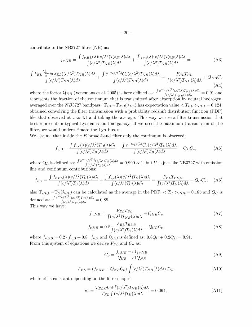
contribute to the NB3727 filter (NB) as:

fν,NB =

∫fν,EL(λ)(c/λ2)TNB(λ)dλ∫

(c/λ2)TNB(λ)dλ+

∫fν,c(λ)(c/λ2)TNB(λ)dλ∫

(c/λ2)TNB(λ)dλ= (A3)

∫FEL

λ2ELc δ(λEL)(c/λ2)TNB(λ)dλ∫

(c/λ2)TNB(λ)dλ+

∫e−τeff (λ)Cν(c/λ2)TNB(λ)dλ∫

(c/λ2)TNB(λ)dλ=

FELTEL∫(c/λ2)TNB(λ)dλ

+QNBCν

(A4)

where the factor QNB (Venemans et al. 2005) is here defined as:∫e−τeff (λ)(c/λ2)TNB(λ)dλ∫

(c/λ2)TNB(λ)dλ= 0.91 and

represents the fraction of the continuum that is transmitted after absorption by neutral hydrogen,

averaged over the NB3727 bandpass. TEL=TNB(λEL) has expectation value < TEL >PDF= 0.124,

obtained convolving the filter transmission with a probability redshift distribution function (PDF)

like that observed at z ' 3.1 and taking the average. This way we use a filter transmission that

best represents a typical Lyα emission line galaxy. If we used the maximum transmission of the

filter, we would underestimate the Lyα fluxes.

We assume that inside the B broad-band filter only the continuum is observed:

fν,B =

∫fν,c(λ)(c/λ2)TB(λ)dλ∫

(c/λ2)TB(λ)dλ=

∫e−τeff (λ)Cν(c/λ2)TB(λ)dλ∫

(c/λ2)TB(λ)dλ= QBCν , (A5)

where QB is defined as:∫e−τeff (λ)(c/λ2)TB(λ)dλ∫

(c/λ2)TB(λ)dλ= 0.999 ∼ 1, but U is just like NB3727 with emission

line and continuum contributions:

fν,U =

∫fν,EL(λ)(c/λ2)TU (λ)dλ∫

(c/λ2)TU (λ)dλ+

∫fν,c(λ)(c/λ2)TU (λ)dλ∫

(c/λ2)TU (λ)dλ=

FELTEL,U∫(c/λ2)TU (λ)dλ

+QUCν , (A6)

also TEL,U=TU (λEL) can be calculated as the average in the PDF, < TU >PDF= 0.185 and QU is

defined as:∫e−τeff (λ)(c/λ2)TU (λ)dλ∫

(c/λ2)TU (λ)dλ= 0.89.

This way we have:

fν,NB =FELTEL∫

(c/λ2)TNB(λ)dλ+QNBCν (A7)

fν,UB = 0.8FELTEL,U∫

(c/λ2)TU (λ)dλ+QUBCν . (A8)

where fν,UB = 0.2 · fν,B + 0.8 · fν,U and QUB is defined as: 0.8QU + 0.2QB = 0.91.

From this system of equations we derive FEL and Cν as:

Cν =fν,UB − c1fν,NBQUB − c1QNB

(A9)

FEL = (fν,NB −QNBCν)

∫(c/λ2)TNB(λ)dλ/TEL (A10)

where c1 is constant depending on the filter shapes:

c1 =TEL,U0.8

∫(c/λ2)TNB(λ)dλ

TEL∫

(c/λ2)TU (λ)dλ= 0.064, (A11)

– 21 –

where the fνs are the observed flux densities, estimated in µJy by us. We estimated the continuum

subtracted emission line flux density as fν,NB − QNBCν = 1.07(fν,NB − fν,UB). To define the

broad-band color U − V , we need to subtract from the U band the contribution of the emission

line in the U transmission filter as:

fν,U,only continuum = fν,U − fELν,U = fν,U −FELTEL,U∫

(c/λ2)TU (λ)dλ.

The UB − NB3727 color is calculated from the ratio of observed fluxes fν,NB and fν,UB. As we

introduced before FEL/fλ,c(λEL) = EWobs, so we replaced FEL = EWobsCν(c/λ2EL), taking into

account the IGM absorption. So:

fν,NB = CνQNB +EWobsCν(c/λ2

EL)TEL∫(c/λ2)TNB(λ)dλ

(A12)

and

fν,UB = CνQUB +0.8 EWobsCν(c/λ2

EL)TEL,U∫(c/λ2)TU (λ)dλ

(A13)

For EWobs = 20× (1+z) = 61 A, hencefν,NBfν,UB

= 1.97.

Therefore:

UB −NB3727 = 2.5 log(fν,NBfν,UB

) > 0.73 (A14)

is the color cut we are using as the first selection criterion of LAEs to select galaxies with rest-frame

EW bigger than 20 A. Plugging equations (A12), (A13) into the equality of (A14), we derive an

expression for

EWobs = A/B, (A15)

where

A = QNB −QUB10((UB−NB3727)/2.5) (A16)

and

B =0.8TEL,U (c/λ2

EL)10((UB−NB3727)/2.5)∫(c/λ2)TU (λ)dλ

−TEL(c/λ2

EL)∫(c/λ2)TNB(λ)dλ

(A17)

In the case in which the EWobs is infinite, for the pure emission line objects, the parts of the

expressions containing EW dominate and the EWobs simplifies, giving a maximum theoretical

value of UB-NB3727 = 2.5 log(15.42) = 2.97. Spurious objects that appear only in the narrow-

band should have infinite UB-NB3727, but may scatter below the maximum theoretical value due

to photometric errors. Real LAEs often have faint continuum, so photometric errors can scatter

their UB-NB3727 color above this theoretical maximum. Hence the maximum cannot be used as a

sharp discriminator between real and fake objects, and it is inevitable that a few objects will appear

to have EWobs =∞. Among our LAEs, 4 of them have these “unphysical” values of UB−NB3727,

consistent with our upper limit on spurious objects found above, but we do not know which of these

objects are truly spurious or simply fell prey to negative noise fluctuations in their UB continua.

In Fig. 4 we associated the value EW=400 A to these 4 objects.

– 22 –

REFERENCES

Adelberger, K. L., Steidel, C. C., Pettini, M., Shapley, A. E., Reddy, N. A., & Erb, D. K. 2005a,

ApJ, 619, 697

Adelberger, K. L., Erb, D. K., Steidel, C. C., Reddy, N. A., Pettini, M., & Shapley, A. E. 2005b,

ApJ, 620, L75

Atek, H., Kunth, D., Schaerer, D., Hayes, M., Deharveng, J. M., Ostlin, G., & Mas-Hesse, J. M.

2009, A&A, 506, L1

Bahcall, N. A., Dong, F., Hao, L., Bode, P., Annis, J., Gunn, J. E., & Schneider, D. P. 2003, ApJ,

599, 814

Bertin, E. & Arnouts, S. 1996, A&AS, 117, 393

Blanc, G. A., Lira, P., Barrientos, L. F., Aguirre, P., Francke, H., Taylor, E. N., Quadri, R.,

Marchesini, D., Infante, L., Gawiser, E., Hall, P. B., Willis, J. P., Herrera, D., & Maza, J.

2008, ApJ, 681, 1099

Bouwens, R. J., Illingworth, G. D., Blakeslee, J. P., & Franx, M. 2006, ApJ, 653, 53

Bruzual, G. & Charlot, S. 2003, MNRAS, 344, 1000

Coil, A. L., Newman, J. A., Croton, D., Cooper, M. C., Davis, M., Faber, S. M., Gerke, B. F.,

Koo, D. C., Padmanabhan, N., Wechsler, R. H., & Weiner, B. J. 2008, ApJ, 672, 153

Dunkley, J., Komatsu, E., Nolta, M. R., Spergel, D. N., Larson, D., Hinshaw, G., Page, L., Bennett,

C. L., Gold, B., Jarosik, N., Weiland, J. L., Halpern, M., Hill, R. S., Kogut, A., Limon, M.,

Meyer, S. S., Tucker, G. S., Wollack, E., & Wright, E. L. 2009, ApJS, 180, 306

Finkelstein, S. L., Rhoads, J. E., Malhotra, S., Grogin, N., & Wang, J. 2008, ApJ, 678, 655

Finkelstein, S. L., Rhoads, J. E., Malhotra, S., & Grogin, N. 2009, ApJ, 691, 465

Francke, H., Gawiser, E., Lira, P., Treister, E., Virani, S., Cardamone, C., Urry, C. M., van

Dokkum, P., & Quadri, R. 2008, ApJ, 673, L13

Gawiser, E., van Dokkum, P. G., Herrera, D., Maza, J., Castander, F. J., Infante, L., Lira, P.,

Quadri, R., Toner, R., Treister, E., Urry, C. M., Altmann, M., Assef, R., Christlein, D.,

Coppi, P. S., Duran, M. F., Franx, M., Galaz, G., Huerta, L., Liu, C., Lopez, S., Mendez,

R., Moore, D. C., Rubio, M., Ruiz, M. T., Toft, S., & Yi, S. K. 2006a, ApJS, 162, 1

Gawiser, E., van Dokkum, P. G., Gronwall, C., Ciardullo, R., Blanc, G. A., Castander, F. J.,

Feldmeier, J., Francke, H., Franx, M., Haberzettl, L., Herrera, D., Hickey, T., Infante, L.,

Lira, P., Maza, J., Quadri, R., Richardson, A., Schawinski, K., Schirmer, M., Taylor, E. N.,

Treister, E., Urry, C. M., & Virani, S. N. 2006b, ApJ, 642, L13

– 23 –

Gawiser, E., Francke, H., Lai, K., Schawinski, K., Gronwall, C., Ciardullo, R., Quadri, R., Orsi,

A., Barrientos, L. F., Blanc, G. A., Fazio, G., Feldmeier, J. J., Huang, J.-S., Infante, L.,

Lira, P., Padilla, N., Taylor, E. N., Treister, E., Urry, C. M., van Dokkum, P. G., & Virani,

S. N. 2007, ApJ, 671, 278

Giavalisco, M., Dickinson, M., Ferguson, H. C., Ravindranath, S., Kretchmer, C., Moustakas, L. A.,

Madau, P., Fall, S. M., Gardner, J. P., Livio, M., Papovich, C., Renzini, A., Spinrad, H.,

Stern, D., & Riess, A. 2004, ApJ, 600, L103

Gronwall, C., Ciardullo, R., Hickey, T., Gawiser, E., Feldmeier, J. J., van Dokkum, P. G., Urry,

C. M., Herrera, D., Lehmer, B. D., Infante, L., Orsi, A., Marchesini, D., Blanc, G. A.,

Francke, H., Lira, P., & Treister, E. 2007, ApJ, 667, 79

Guhathakurta, P., Tyson, J. A., & Majewski, S. R. 1990, ApJ, 357, L9

Hildebrandt, H., Erben, T., Dietrich, J. P., Cordes, O., Haberzettl, L., Hetterscheidt, M., Schirmer,

M., Schmithuesen, O., Schneider, P., Simon, P., & Trachternach, C. 2006, A&A, 452, 1121

Hildebrandt, H., Pielorz, J., Erben, T.., van Waerbeke, L., Simon, P., & Capak, P. 2009, A&A,

498, 725

Hogg, D. W., Cohen, J. G., Blandford, R., & Pahre, M. A. 1998, ApJ, 504, 622

Kovac, K., Somerville, R. S., Rhoads, J. E., Malhotra, S., & Wang, J. 2007, ApJ, 668, 15

Lai, K., Huang, J.-S., Fazio, G., Gawiser, E., Ciardullo, R., Damen, M., Franx, M., Gronwall, C.,

Labbe, I., Magdis, G., & van Dokkum, P. 2008, ApJ, 674, 70

Landy, S. D. & Szalay, A. S. 1993, ApJ, 412, 64

Lee, K., Giavalisco, M., Gnedin, O. Y., Somerville, R. S., Ferguson, H. C., Dickinson, M., & Ouchi,

M. 2006, ApJ, 642, 63

Lehmer, B. D., Brandt, W. N., Alexander, D. M., Bauer, F. E., Schneider, D. P., Tozzi, P., Bergeron,

J., Garmire, G. P., Giacconi, R., Gilli, R., Hasinger, G., Hornschemeier, A. E., Koekemoer,

A. M., Mainieri, V., Miyaji, T., Nonino, M., Rosati, P., Silverman, J. D., Szokoly, G., &

Vignali, C. 2005, ApJS, 161, 21

Luo, B., Bauer, F. E., Brandt, W. N., Alexander, D. M., Lehmer, B. D., Schneider, D. P., Brusa,

M., Comastri, A., Fabian, A. C., Finoguenov, A., Gilli, R., Hasinger, G., Hornschemeier,

A. E., Koekemoer, A., Mainieri, V., Paolillo, M., Rosati, P., Shemmer, O., Silverman, J. D.,

Smail, I., Steffen, A. T., & Vignali, C. 2008, ApJS, 179, 19

Madau, P. 1995, ApJ, 441, 18

Madau, P., Pozzetti, L., & Dickinson, M. 1998, ApJ, 498, 106

– 24 –

Neufeld, D. A. 1991, ApJ, 370, L85

Nilsson, K. K., Møller, P., Moller, O., Fynbo, J. P. U., Micha lowski, M. J., Watson, D., Ledoux,

C., Rosati, P., Pedersen, K., & Grove, L. F. 2007, A&A, 471, 71

Nilsson, K. K., Tapken, C., Møller, P., Freudling, W., Fynbo, J. P. U., Meisenheimer, K., Laursen,

P., & Ostlin, G. 2009, A&A, 498, 13

Ono, Y., Ouchi, M., Shimasaku, K., Akiyama, M., Dunlop, J., Farrah, D., Lee, J. C., McLure, R.,

Okamura, S., & Yoshida, M. 2009, ArXiv e-prints

Orsi, A., Lacey, C. G., Baugh, C. M., & Infante, L. 2008, MNRAS, 391, 1589

Ouchi, M., Shimasaku, K., Furusawa, H., Miyazaki, M., Doi, M., Hamabe, M., Hayashino, T.,

Kimura, M., Kodaira, K., Komiyama, Y., Matsuda, Y., Miyazaki, S., Nakata, F., Okamura,

S., Sekiguchi, M., Shioya, Y., Tamura, H., Taniguchi, Y., Yagi, M., & Yasuda, N. 2003, ApJ,

582, 60

Ouchi, M., Shimasaku, K., Okamura, S., Furusawa, H., Kashikawa, N., Ota, K., Doi, M., Hamabe,

M., Kimura, M., Komiyama, Y., Miyazaki, M., Miyazaki, S., Nakata, F., Sekiguchi, M.,

Yagi, M., & Yasuda, N. 2004, ApJ, 611, 685

Ouchi, M., Hamana, T., Shimasaku, K., Yamada, T., Akiyama, M., Kashikawa, N., Yoshida, M.,

Aoki, K., Iye, M., Saito, T., Sasaki, T., Simpson, C., & Yoshida, M. 2005, ApJ, 635, L117

Ouchi, M., Shimasaku, K., Akiyama, M., Simpson, C., Saito, T., Ueda, Y., Furusawa, H., Sekiguchi,

K., Yamada, T., Kodama, T., Kashikawa, N., Okamura, S., Iye, M., Takata, T., Yoshida,

M., & Yoshida, M. 2008, ApJS, 176, 301

Pentericci, L., Grazian, A., Fontana, A., Castellano, M., Giallongo, E., Salimbeni, S., & Santini, P.

2009, A&A, 494, 553

Pickles, A. J. 1998, PASP, 110, 863

Pirzkal, N., Malhotra, S., Rhoads, J. E., & Xu, C. 2007, ApJ, 667, 49

Quadri, R., van Dokkum, P., Gawiser, E., Franx, M., Marchesini, D., Lira, P., Rudnick, G., Herrera,

D., Maza, J., Kriek, M., Labbe, I., & Francke, H. 2007, ApJ, 654, 138

Ranalli, P., Comastri, A., & Setti, G. 2003, A&A, 399, 39

Schaerer, D. & Verhamme, A. 2008, A&A, 480, 369

Schlegel, D. J., Finkbeiner, D. P., & Davis, M. 1998, ApJ, 500, 525

Shapley, A. E., Steidel, C. C., Adelberger, K. L., Dickinson, M., Giavalisco, M., & Pettini, M. 2001,

ApJ, 562, 95

– 25 –

Shapley, A. E., Steidel, C. C., Pettini, M., & Adelberger, K. L. 2003, ApJ, 588, 65

Sheth, R. K. & Tormen, G. 1999, MNRAS, 308, 119

Simon, P. 2007, A&A, 473, 711

Somerville, R. S., Lee, K., Ferguson, H. C., Gardner, J. P., Moustakas, L. A., & Giavalisco, M.

2004, ApJ, 600, L171

Steidel, C. C. & Hamilton, D. 1992, AJ, 104, 941

Steidel, C. C., Adelberger, K. L., Giavalisco, M., Dickinson, M., & Pettini, M. 1999, ApJ, 519, 1

Steidel, C. C., Adelberger, K. L., Shapley, A. E., Pettini, M., Dickinson, M., & Giavalisco, M. 2003,

ApJ, 592, 728

Steidel, C. C., Shapley, A. E., Pettini, M., Adelberger, K. L., Erb, D. K., Reddy, N. A., & Hunt,

M. P. 2004, ApJ, 604, 534

Stiavelli, M., Scarlata, C., Panagia, N., Treu, T., Bertin, G., & Bertola, F. 2001, ApJ, 561, L37

Tapken, C., Appenzeller, I., Noll, S., Richling, S., Heidt, J., Meinkohn, E., & Mehlert, D. 2007,

A&A, 467, 63

Treister, E., Urry, C. M., Chatzichristou, E., Bauer, F., Alexander, D. M., Koekemoer, A., Van

Duyne, J., Brandt, W. N., Bergeron, J., Stern, D., Moustakas, L. A., Chary, R.-R., Conselice,

C., Cristiani, S., & Grogin, N. 2004, ApJ, 616, 123

van Dokkum, P. G. 2001, PASP, 113, 1420

Venemans, B. P., Rottgering, H. J. A., Miley, G. K., Kurk, J. D., De Breuck, C., Overzier, R. A.,

van Breugel, W. J. M., Carilli, C. L., Ford, H., Heckman, T., Pentericci, L., & McCarthy,

P. 2005, A&A, 431, 793

Verhamme, A., Schaerer, D., & Maselli, A. 2006, A&A, 460, 397

Verhamme, A., Schaerer, D., Atek, H., & Tapken, C. 2008, A&A, 491, 89

Virani, S. N., Treister, E., Urry, C. M., & Gawiser, E. 2006, AJ, 131, 2373

Zehavi, I., Zheng, Z., Weinberg, D. H., Frieman, J. A., Berlind, A. A., Blanton, M. R., Scoccimarro,

R., Sheth, R. K., Strauss, M. A., Kayo, I., Suto, Y., Fukugita, M., Nakamura, O., Bahcall,

N. A., Brinkmann, J., Gunn, J. E., Hennessy, G. S., Ivezic, Z., Knapp, G. R., Loveday, J.,

Meiksin, A., Schlegel, D. J., Schneider, D. P., Szapudi, I., Tegmark, M., Vogeley, M. S., &

York, D. G. 2005, ApJ, 630, 1

This preprint was prepared with the AAS LATEX macros v5.2.

– 26 –

Fig. 1.— Transmission curve of the NB3727 narrow-band filter (blue) at MOSAIC II and of the

U (magenta) and B (cyan) broad-band filters at WFI. The filter transmission curves have been

multiplied by the detector quantum efficiency and the atmospheric transmission at one airmass. A

typical Lyα galaxy template is also shown in black.

– 27 –

Fig. 2.— Left panel: UB-NB3727 color versus NB3727 magnitude. Black points represent the

total sample of 19455 sources, while the red circles represent the LAE candidates. The horizontal

red line represents the cut at rest-frame equivalent width bigger than 20 A (UB-NB3727> 0.73).

The vertical line represent the 5σ detection limit of the survey at NB3727 = 25.1. Right panel:

UB-NB3727 color distribution for those objects in the initial catalog with 24<NB3727<25.1. The

Gaussian fit is obtained considering the range -0.5≤UB-NB3727≤0.5. The σ of the best fit Gaussian

curve is 0.2. This means that our color cut UB-NB3727>0.73 is selecting objects above 3.5σ.

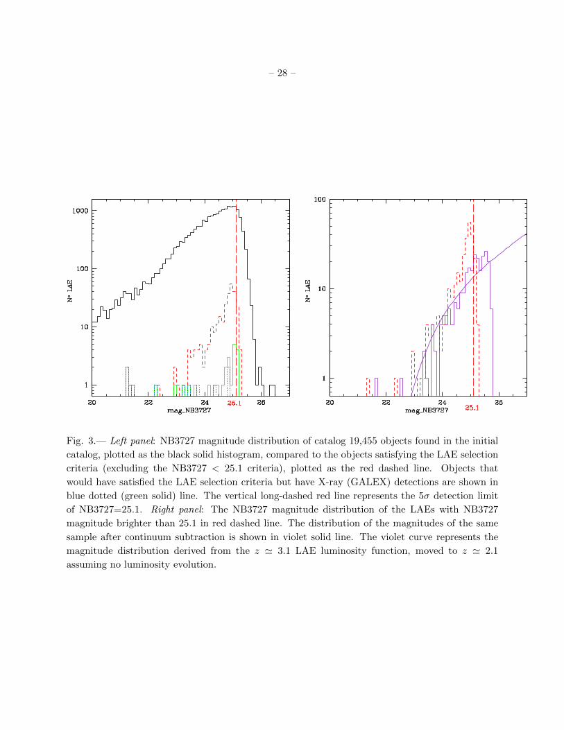
– 28 –

Fig. 3.— Left panel: NB3727 magnitude distribution of catalog 19,455 objects found in the initial

catalog, plotted as the black solid histogram, compared to the objects satisfying the LAE selection

criteria (excluding the NB3727 < 25.1 criteria), plotted as the red dashed line. Objects that

would have satisfied the LAE selection criteria but have X-ray (GALEX) detections are shown in

blue dotted (green solid) line. The vertical long-dashed red line represents the 5σ detection limit

of NB3727=25.1. Right panel: The NB3727 magnitude distribution of the LAEs with NB3727

magnitude brighter than 25.1 in red dashed line. The distribution of the magnitudes of the same

sample after continuum subtraction is shown in violet solid line. The violet curve represents the

magnitude distribution derived from the z ' 3.1 LAE luminosity function, moved to z ' 2.1

assuming no luminosity evolution.

– 29 –

Fig. 4.— Left panel: Rest-frame equivalent width (EW) versus logarithmic Lyα luminosity for

our sample of 250 z ' 2.1 LAEs in red triangles and the sample of 154 z ' 3.1 LAEs in blue

squares. The solid lines represent the 5σ detection limit in magnitude of the samples, in red for

the z ' 2.1 LAE survey and in blue for the z ' 3.1 survey. At log(L(Lyα)) ≥ 42.1 the z ' 2.1

sample appears to be unbiased in the sense of rest-frame EW versus Lyα luminosity. The black

horizontal line represents the cut at rest-frame EW > 20 A. Right panel: Distribution of rest-frame

equivalent widths for the z ' 2.1 LAEs with log(L(Lyα)) ≥ 42.1. The black solid line represents

its exponential best-fit. In cyan dashed line we show the best-fit exponential for z ' 3.1 LAEs

from Gronwall et al. (2007) and in orange dotted line we show the best-fit exponential for z ' 2.3

LAEs from Nilsson et al. (2009). The magenta long-dashed line represents the Gaussian fit of the

histogram. As a comparison we show the Gaussian fit by Ouchi et al. (2008) as the lower blue

dotted line. The bin at EW = 400 A includes formally infinite EW estimations i.e., objects whose

continuum photometry is dimmer than should be possible even for a pure emission line, although

this can be caused by photometric noise.

– 30 –

Fig. 5.— SFR(UV) versus SFR(Lyα), also labeled with R mag versus monochromatic NB3727

flux for our sample of 250 LAEs. The vertical dashed line represents the limit flux of the survey

(estimated using the maximum transmission filter value and rest-frame EW= 20 A), while the

dash-dotted line represents 90% completeness limit. The diagonal dotted line represents the case in

which SFR(UV)=SFR(Lyα). The magenta dashed line represents the case in which the SFR(UV) is

equal to the SFR(Lyα)× the median-ratio(SFR(UV)/SFR(Lyα) = 1.5), for the part of the sample

that is complete. The points at R = 30 represent objects for which the measured flux in R band is

negative. The reduced density of objects at the upper left (SFR(UV)> 10 Myr−1) and lower left

(SFR(UV)< 2 M yr−1 and SFR(Lyα)< 1 M yr−1) of the plot is at least partially caused by our

rest-frame EW>20A and 5σ detection limit selections.

– 31 –

Fig. 6.— Left panel: Broad-band R magnitude as function of B − R color. The median value of

B − R and median photometric uncertainty in each 0.5 R magnitude bin are shown by triangles

and error bars respectively. For R ≥ 27 the median B − R = −0.9 ± 1.4 and it is represented by

the lower triangle and its error bar. Right panel: B−R color distribution. The vertical dashed line

represents B −R = 1 below which there are the colors of the majority of the LAEs in our sample.

Fig. 7.— Left panel: R magnitude distribution of the LAE sample. The vertical dashed line is

drawn at R = 25. Right panel: Two-color diagram for R < 25 (blue) and R > 25 (red). Red

(blue) error bars show median Ucorr − V and V −R colors and uncertainties of the faint (bright)

subsamples. Cyan points are z < 1.4 MUSYC spectroscopic catalog objects.

– 32 –

ó ó

ó

ó

ó

óóóó

ó

óó ó ó

ó

óóó

ó

ó

0 200 400 600 800

0.0

0.5

1.0

Θ @arcsecD

ΩLA

EHΘL

Fig. 8.— Upper panel: Declination versus right ascension plot, showing the spatial distribution of

the 250 LAEs. Lower panel: Angular correlation function generated from our sample of 250 LAEs

in black triangles. The blue solid curve is the best power law fit to the data, calculated from 40

to 600 arcsec. This range is chosen to avoid the 1-halo term at small scales and to avoid sampling

noise at big scales.

– 33 –

äø

ø

ø

ø

ø

è

è

ø

ø

ø

ø

ø

ç

çç

ç

ç

ää

ø

ø

ø

ø

ø

èèèè

øø

ì

ì

ì

ì

This Result

Ga07,LAE

F08,LBG

Q07,DRG

Q07,K<21

sBzK

B08,pBzK

A05a

A05a

A05bK<20.5

A05b20.5<K<21.5

A05bK>21.5

L06

L06z<26

L06z<26.5

K07

Ou03

Ou04i<26

Ou04z<25.8

H09

H09i<26

H09z<26.5

0.1 L*0.4 L*

2.5 L*

6.0 L*

Rich Clusters

C08 Red

C08Blue

1.0 L*

0 1 2 3 4 50

1

2

3

4

5

6

7

redshift

bias

fact

or

Fig. 9.— Bias evolution in redshift for a variety of galaxy populations. Stars are galaxies selected

from their UV colors/magnitudes, diamonds are K selected, filled circles are narrow-band selected

and open circles are low-redshift samples. The result from this work at z ' 2.1 is plotted in green

assuming a contamination fraction of 7±7%, together with the MUSYC LAE result from Gawiser

et al. (2007) at z ' 3.1 (G07). Other results from MUSYC are also in color, namely: LBGs at z ∼ 3

in blue (F08) from Francke et al. (2008), K-selected galaxies and Distant Red Galaxies (DRG) at

z ' 2.6 from Quadri et al. (2007) (Q07), and both passive and star-forming, BzK-selected galaxies

from Blanc et al. (2008) (B08), in orange. The labels for other literature results correspond to:

z ' 1.7 color selected galaxies and LBG (A05a) from Adelberger et al. (2005a), z ' 2.1 color

selected galaxies divided by their K magnitude (A05b) from Adelberger et al. (2005b), LBGs at

z ' 3, z ' 4, z ' 5 (L06, H09) from Lee et al. (2006) and from Hildebrandt et al. (2009), LBGs

at z ' 4 and 5 (Ou04) from Ouchi et al. (2004), high-z LAE measurements (Ou03, K07) from

Ouchi et al. (2003) and Kovac et al. (2007). At intermediate redshift, z ∼ 1, galaxies separated

by color (C08) come from Coil et al. (2008). Low redshift (z ∼ 0) galaxies, labeled by their

optical luminosity, come from Zehavi et al. (2005) and the single point for rich galaxy clusters from

Bahcall et al. (2003). The dashed line corresponds to conditional mass function trajectories for

bias evolution from Sheth & Tormen theory.

– 34 –

Table 1. LOG OF ALL BANDS

Band Telescope Exposure Time(s) 5σ detection limit

NB3727 4m CTIO 128700 25.1

U 2.2m La Silla 78891 26.1

B 2.2m La Silla 69431 26.9

V 2.2m La Silla 104603 26.5

R 2.2m La Silla 87653 26.5

Table 2. LOG OF NARROW BAND OBSERVATIONS

(UT) starting date NB Exposure (s) Seeing FWHM (′′) Conditions

2007 Dec., 3rd 10800 1.4 Full nt, cloudless

2007 Dec., 4rd 7200 1.5 Half nt, cloudless

2007 Dec., 5th 21600 1.3 Full nt, cloudless

2007 Dec., 6th 10800 1.3 Half nt, cloudless

2007 Dec., 7th 21600 1.4 Full nt, cloudless

2007 Dec., 8th 10800 1.7 Half nt, cloudless

2007 Dec., 9th 18000 1.6 Full nt, cloudless

2007 Dec., 10th 3600 1.1 Half nt, cloudless

2007 Dec., 11th 14400 1.2 Full nt, cloudless

2007 Dec., 12th 9900 1.3 Half nt, cloudless

Note. — The seeing here reported is the mean of the mode of the seeing estimations

for each night.

Full nt = full night allocated

Half nt = second half of the night allocated

– 35 –

Table 3. LOG OF NARROW BAND IMAGES PROPERTIES

image airmass MSCSCALE skyRMS seeing (′′) weight

3dec 1 1.002 1.000 7.97 1.35 0.00858

3dec 2 1.042 1.037 8.11 1.26 0.00871

3dec 3 1.154 1.128 8.68 1.63 0.00376

4dec 1 1.066 1.215 7.20 1.59 0.00500

4dec 2 1.203 1.305 7.44 1.46 0.00493

5dec 1 1.091 1.199 6.16 1.65 0.00642

5dec 2 1.016 1.149 6.34 1.23 0.01207

5dec 3 1.003 1.168 6.74 1.18 0.01104

5dec 4 1.051 1.203 6.84 1.16 0.01034

5dec 5 1.172 1.287 7.21 1.29 0.00687

5dec 6 1.411 1.470 7.71 1.39 0.00400

6dec 1 1.072 1.178 7.14 1.42 0.00697

6dec 2 1.218 1.257 7.59 1.30 0.00641

6dec 3 1.504 1.472 8.27 1.34 0.00373

7dec 1 1.104 1.055 8.16 1.62 0.00495

7dec 2 1.019 1.044 8.24 1.44 0.00647

7dec 3 1.003 1.056 8.64 1.41 0.00600

7dec 4 1.049 1.073 8.92 1.32 0.00619

7dec 5 1.168 1.000 8.87 1.14 0.00979

7dec 6 1.404 1.135 9.66 1.22 0.00589

8dec 1 1.099 1.062 7.95 1.44 0.00752

8dec 2 1.268 1.184 8.15 1.60 0.00463

8dec 3 1.599 1.505 8.76 2.06 0.00130

9dec 1 1.093 1.00 7.51 1.60 0.00761

9dec 2 1.016 0.987 7.23 1.57 0.00881

9dec 3 1.003 0.994 7.17 1.63 0.00814

9dec 4 1.003 1.014 7.66 1.38 0.00961

9dec 5 1.169 1.092 8.16 1.64 0.00512

10dec 1 1.435 1.184 8.29 1.14 0.00800

11dec 1 1.001 0.969 6.40 0.99 0.02291

11dec 2 1.036 1.003 6.55 0.97 0.02072

11dec 3 1.143 1.067 6.65 1.30 0.01279

11dec 4 1.356 1.208 6.79 1.53 0.00706

– 36 –

Table 3—Continued

image airmass MSCSCALE skyRMS seeing (′′) weight

12dec 1 1.142 1.073 7.40 0.99 0.01397

12dec 2 1.355 1.216 7.84 1.21 0.00786

12dec 3 1.775 1.989 6.98 1.57 0.00233

– 37 –

Tab

le4.

Pro

per

ties

ofL

AE

sb

inn

edby

conti

nu

um

mag

nit

ud

e

Rm

inR

max

nu

mb

erof

ob

ject

sB

-RU

corr

-VV

-RU

B-N

B3727

EWrestframe

SF

R(L

yα

)S

FR

(UV

)

-24.0

15

0.6±

0.7

1.1±

1.0

0.1±

0.5

1.0±

0.2

30±

13

1.5±

7.4

15.6±

12.3

24.0

24.5

20

0.5±

0.4

1.2±

0.6

0.3±

0.2

0.8±

0.2

25±

11

1.0±

1.5

10.0±

1.5

24.5

25.0

51

0.4±

0.3

0.9±

0.4

0.2±

0.2

0.9±

0.2

28±

11

1.0±

0.6

6.6±

0.8

25.0

25.5

62

0.2±

0.2

0.7±

0.5

0.1±

0.2

1.0±

0.3

32±

30

1.0±

0.9

4.1±

0.6

25.5

26.0

39

0.1±

0.3

0.6±

0.5

0.0±

0.2

1.2±

0.4

43±

48

1.1±

0.7

2.8±

0.4

26.0

26.5

25

-0.0±

0.2

0.5±

0.7

0.1±

0.4

1.7±

0.3

96±

51

1.4±

1.1

1.7±

0.2

26.5

27.0

19

-0.0±

0.8

-0.1±

0.7

0.1±

0.4

1.7±

0.4

101±

130

1.5±

0.4

1.1±

0.2

27.0

-19

-0.3±

1.4

-0.2±

1.5

-0.6±

1.7

2.0±

1.1

150±

456

1.5±

0.2

0.4±

0.3

Note

.—

Th

eR

,B

-R,

Uco

rr-V

,V

-R,

UB

-NB

3727,

EW

(A)

an

dS

FR

s(M

yr−

1)

are

the

med

ian

inth

eR

magn

itu

de

bin

sin

the

ran

ge

bet

wee

nR

min

an

dR

max.

Th

eer

rors

show

nare

the

stan

dard

dev

iati

on

inea

chb

in.