Lyapunov stability analysis for nonlinear delay systems under ...

Almutairi et al. Advances in Difference Equations (2021) 2021:186 https://doi.org/10.1186/s13662-021-03344-6

R E S E A R C H Open Access

Lyapunov stability analysis for nonlineardelay systems under random effects andstochastic perturbations with applications infinance and ecologyAbdulwahab Almutairi1, H. El-Metwally2, M.A. Sohaly2* and I.M. Elbaz2,3

*Correspondence:[email protected] Department, Facultyof Science, Mansoura University,Mansoura, EgyptFull list of author information isavailable at the end of the article

AbstractThis manuscript is involved in the study of stability of the solutions of functionaldifferential equations (FDEs) with random coefficients and/or stochastic terms. Wefocus on the study of different types of stability of random/stochastic functionalsystems, specifically, stochastic delay differential equations (SDDEs). Introducingappropriate Lyapunov functionals enables us to investigate the necessary conditionsfor stochastic stability, asymptotic stochastic stability, asymptotic mean squarestability, mean square exponential stability, global exponential mean square stability,and practical uniform exponential stability. Some examples with numericalsimulations are presented to strengthen the theoretical results. Using our theoreticalstudy, important aspects of epidemiological and ecological mathematical models canbe revealed. In ecology, the dynamics of Nicholson’s blowflies equation is studied.Conditions of stochastic stability and stochastic global exponential stability of theequilibrium point at which the blowflies become extinct are investigated. In finance,the dynamics of the Black–Scholes market model driven by a Brownian motion withrandom variable coefficients and time delay is also studied.

Keywords: Stochastic delay models; Stochastic stability; Mean square stability;Practical uniform stability; Exponential stability; Nicholson’s blowflies model;Black–Scholes market model

1 IntroductionMany applications in many disciplines assume that the future state of the system is inde-pendent of the past states and is only determined by the current state. This is known asthe causality principle which is only an approximation to the true situation of the system.Consequently, it is practical to consider the past states of the system. A real system shouldbe modeled by differential equations involving delays in time [1, 2]. The past dependencehas been assumed in the differential equation through the state variable and not its deriva-tive. Hence, this paper focuses on the retarded (delayed) differential equations (DDEs) in

© The Author(s) 2021. This article is licensed under a Creative Commons Attribution 4.0 International License, which permits use,sharing, adaptation, distribution and reproduction in any medium or format, as long as you give appropriate credit to the originalauthor(s) and the source, provide a link to the Creative Commons licence, and indicate if changes were made. The images or otherthird party material in this article are included in the article’s Creative Commons licence, unless indicated otherwise in a credit lineto the material. If material is not included in the article’s Creative Commons licence and your intended use is not permitted bystatutory regulation or exceeds the permitted use, you will need to obtain permission directly from the copyright holder. To view acopy of this licence, visit http://creativecommons.org/licenses/by/4.0/.

Almutairi et al. Advances in Difference Equations (2021) 2021:186 Page 2 of 32

the form

dx(t)dt

= μ(t, x(t), xt

). (1)

For h > 0, let C := C([–h, 0],Rn) denote a Banach space of continuous functions: [–h, 0] →R

n with respect to the supremum norm ‖φ‖ := sups∈[–h,0] |φ(s)|. In (1), xt := x(t + s), –h ≤s ≤ 0, and the initial history function is

x(t0) = φ, φ ∈ C([–h, 0]

). (2)

Equation (1) with (2) is involved in many interesting mathematical problems. Different de-lay differential equations are primarily taken from ecological and financial science litera-ture. There are many disciplines such as, but not limited to, population dynamics, ecology,economy, and neural networks [2, 3]. Many recent works dedicated to the delay differentialequations and the fractional differential equations can be found in [4–13]. Many numeri-cal studies dedicated to fractional models in epidemiology can be found in [14–17].

The deterministic models do not preserve the natural uncertainty of the dynamicsof the system, whereas the random/stochastic systems preserve all types of the uncer-tainty. Stochastic delay differential equations can be considered as DEs with random ele-ments and/or stochastic terms with time delays. In this paper, we propose the uncertaintythrough perturbing the system by the Brownian motion or through assuming that the co-efficients, initial conditions, and forcing terms are random variables or stochastic terms.We shall insert the stochastic term involving the Brownian motion, and this technique isa kind of non-parametric stochastic perturbation, then (1)–(2) become

⎧⎨

⎩dx(t) = μ(t, xt) dt + σ (t, xt) dB(t), xt := x(t + s), –h < s ≤ t0,

x(t0) = φ, φ ∈ C([–h, 0]).(3)

This system describes the real world problems in an effective way. SDDEs have beenapplied in biology, finance, neural networks, ecology, etc. Many works can be found in[18, 19]. The probabilistic behavior of x(t) in (3) is restricted to a specific pattern which isGaussian distribution as the source of randomness is the Wiener process. In (3), μ,σ arecontinuous functionals defined on [t0,∞) ×C([–h, 0]) and are assumed to satisfy the localLipschitz condition, i.e., for L > 0, |μ1(t, xt) – μ1(t, x∗

t )| ≤ L|xt – x∗t |, obviously, | ∂μ(t,xt )

∂x | < L,and also for σ . The stochastic process B(t) : [t0,∞) → R is a one-dimensional Brownianmotion defined on the complete probability space (�,F ,FB

t ,P), where FBt is the filtration

generated by it up to time t [20].We will also discuss the random delay differential equations (RDDEs) with discrete delay

τ > 0 in the form

dx(t,ω) = μ(t,ω, x(t,ω), x(t – τ ,ω)

)dt, (4)

where ω belongs to the underlying probability space (�,F ,P). Via the outcome ω, the un-certainty is introduced. This is another way to introduce the uncertainty by assuming thatthe inputs (coefficients, initial conditions, forcing terms, etc.) are random variables and/orstochastic processes. In this case, we have a wider type of probability distributions such

Almutairi et al. Advances in Difference Equations (2021) 2021:186 Page 3 of 32

as Gaussian, gamma, beta, binomial, etc. And this provides a great flexibility in dealingwith the real life applications. Many applications regarding the RDDEs can be found in[21–24].

Many authors have studied the existence and uniqueness of the stochastic delay differen-tial equations, for more details, see [25]. The SDDE has a unique global solution x(t, t0,φ)for any given initial history function x0 = φ ∈ C([–h, 0]). Our study assumes two importantassumptions as follows.

Assumption 1 Assume that the two functionals μ and σ satisfy the following conditions:

μ(t, 0) = 0, σ (t, 0) = 0.

Then system (3) admits the trivial solution, and hence stochastic stability, mean squarestability, and global mean square exponential stability have received very much attention.

If the origin is not the equilibrium point, then practical stability guarantees the stabilityand boundedness of all paths in a certain ball of the center at the origin.

Assumption 2 For practical global uniform stability, if μ and σ satisfy

μ(t, 0) �= 0, σ (t, 0) �= 0,

then our study of stability of SDDE will be in a small neighborhood (ball Br) of the origin.

Constructing appropriate Lyapunov functions/functionals is an effective way in thestudy of stability of deterministic and stochastic systems, more details can be found in[18, 25, 26]. Introducing suitable Lyapunov functionals implies various types of stabilitywith different stability conditions. This manuscript uses the Lyapunov functionals to in-vestigate the asymptotic stochastic stability, global mean square exponential stability ofthe zero solution of (3). And practical stability of (3) is also studied when the origin isnot necessarily an equilibrium point. It is worthy to study the global exponential meansquare stability while many researchers did not. Regardless of the initial history functionof the system, global exponential stability makes any trajectory tend to the attractor of thesystem. Moreover, the paper discusses the asymptotic mean square stability of (3) withrandom coefficients. Many works regarding the stability of random/stochastic dynamicalsystems are considered in [27–29].

With regard to the applications, the main application in our manuscript is Nicholson’sblowflies equation perturbed by white noise. This model is one of the major problems inecology which describes the dynamics of the population of the Australian sheep blowfly,Lucilia cuprina, which is known as Nicholson’s blowfly. The author in [30] introduced thedifferential equation that models the population dynamics of this blowfly with delay in theform

dx(t)dt

= px(t – τ )e–ax(t–τ ) – δx(t), (5)

where x(t) is the population of the mature adults at time t. All parameters p, a, δ ∈ [0,∞),where p represents the maximum daily production rate of eggs per capita, a–1 is the size

Almutairi et al. Advances in Difference Equations (2021) 2021:186 Page 4 of 32

at which the population reproduces at the maximum rate, δ is the adult death rate of percapita daily, and τ > 0 is the delay in the production process.

Model (5) admits only the trivial solution (x = 0) if the basic reproduction ratio of thesystem R0 < 1, where R0 = p

δ. The species become extinct due to the global stability of the

zero solution of (5), see [31]. Many authors have studied the dynamics of this equation[31–35], and stochastically [36–38].

We shall introduce the necessary and sufficient conditions for stochastic stability andstochastic global exponential stability of the trivial equilibrium of (5) under the influenceof Brownian motion.

Moreover, we study the Black–Scholes delay market model driven by a Brownian motionwith random variable coefficients. This model has become the most known way to modelpricing options in financial markets. It was shown firstly in 1973 by [39]. Many authorshave studied the stochastic volatility of this model, see [40–42]. Generally, the stability ofa stochastic fractional Black–Scholes market model has been studied by [43], for example.

For the numerical simulation, this paper uses the algorithm of an Euler–Maruyamascheme which was shown by [44]. The solution of (3) can be written in the integral form

x(t) = φ +∫ t

t0

μ(s, x(s), xs

)ds +

∫ t

t0

σ(s, x(s), xs

)dB(s). (6)

The last integral is called an Itô stochastic integral. B(t) is discretized by dividing the inter-val [0, T] into N sub-intervals, then t = T

N . And Bn = Btn+1 –Btn , where Bn ∼ N(0,t).Then the stochastic integral

∫ T0 σ (s, x) dB(s) ≈ ∑N

n=0 σ (tn, xn)(Btn+1 – Btn ). The step size tmust be small enough for better numerical approximations. From solution (6),

∫ tn+1

tn

μ(s, x) ds ≈ μ(tn, xn)t and∫ tn+1

tn

σ (s, x) dB(s) ≈ σ (tn, xn)Bn.

Then, the Euler–Maruyama scheme has the form

xn+1 = xn + μ(tn, xn)t + σ (tn, xn)Bn. (7)

x(tn) is the data required in the scheme and x(tn+1) is the resulting process at tn+1. TheEM scheme is strongly convergent with order 0.5, i.e., if we want to decrease the error 10times, the step size should be smaller 100 times. t cannot be too small because of timeand the computational errors. [45] studied the convergence rate of this scheme. There arealternative numerical schemes like the Milstein scheme (which is more accurate becauseof the second order “correction” term added to the scheme), firstly shown by [46], and theRunge–Kutta scheme. With order 1, these schemes are strongly convergent, i.e., by reduc-ing the error 10 times, t must be smaller 10 times. The Runge–Kutta scheme requirescomputing the derivatives, so we avoid it at present.

This manuscript is organized as follows. Section 2 is devoted to some important pre-liminaries. A rigorous mathematical study of stability with proofs of some important the-orems is presented in Sect. 3. Stability of the stochastic Nicholson’s blowflies model andthe Black–Scholes model with random coefficients is presented in Sect. 4. Some numeri-cal examples with stability regions and computer simulations are shown in Sect. 5. Resultsand discussions are presented in Sect. 6.

Almutairi et al. Advances in Difference Equations (2021) 2021:186 Page 5 of 32

2 PreliminariesNotations ([20, 47–49])

1. Define Sh = {x ∈Rn,‖x‖ < h} and K as the family of all continuous nondecreasing

functions υ : R+ →R+ such that υ(x) > 0∀x > 0 and υ(0) = 0.2. L2

Ft{�;R} is the family of R-valued Ft-measurable random variables ζ such that

E|ζ |2 < ∞.3. L2{[a, b];R} is the family of R-valued Ft-adapted square-integrable processes

{X(t)}a≤t≤b such that

∫ b

a

∣∣X(t)∣∣2 dt < ∞, a.s.

4. Let M2([0, T],R) denote the family of processes in L2{[a, b];R} such that

E

(∫ b

a

∣∣X(t)∣∣2 dt

)< ∞.

Definition 2.1 ([26]) The Lyapunov function V(t, x) defined on [t0,∞) × Sh is positivedefinite if V(t, 0) ≡ 0, and V(t, x) ≥ υ(x) for all (t, x) ∈ [0,∞) × Sh, where υ(x) ∈ K. TheLyapunov function V(t, x) is negative definite if –V(t, x) is positive definite.

Definition 2.2 ([26]) The positive definite function υ(‖x(t)‖) is radially unbounded ifυ(‖x(t)‖) → ∞ as x → ∞. The Lyapunov functional V(t, xt) is positive definite and ra-dially unbounded if there exists υ(‖x(t)‖) such that V(t, xt) ≥ υ(‖x(t)‖).

The zero-mean property of the stochastic integral in (6) is useful, so we state withoutproof this property in the next theorem, and the proof is stated in [50].

Theorem 2.1 Let X(t) ∈M2([0, T],R), i.e., E∫ b

a |X(s)|2 ds < ∞. Then, for 0 ≤ t0 ≤ t1 < T ,

E

(∫ t1

t0

X(s) dBs

)= 0.

Define the differential operator L associated with (3) by

L =∂

∂t+

n∑

i=1

μi∂

∂xi+

12

n∑

i,j=1

[σ T · σ ]

i,j∂2

∂xi∂xj.

This operator can be applied to the Lyapunov function V(t, xt) : [t0,∞) × Sh →R+, then

LV(t, xt) =∂V∂t

+ μT ∂V∂x

+12

Tr[σ T ∂2

∂x2 σ

], (8)

which is called an Itô formula, T is the transposition, and Tr is the trace of the matrix.

Definition 2.3 ([22]) Let X, Y be random variables, for real numbers n > 1, m > 1 with1n + 1

m = 1,

E[|XY |] ≤ (

E[Xn]) 1

n(E

[Y m]) 1

m , (9)

Almutairi et al. Advances in Difference Equations (2021) 2021:186 Page 6 of 32

which is called Hölder’s inequality. In particular, for n = m = 2, we have the Cauchy–Schwarz inequality. For square-integrable functions f , g on [a, b],

∣∣∣∣

∫ b

af (x)g(x) dx

∣∣∣∣ ≤

(∫ b

af 2(x) dx

) 12(∫ b

ag2(x) dx

) 12

.

Lemma 2.1 ([51]) Let σ (t, xt) : [t0,∞) ×C[–h, 0] and let α,β , T be arbitrary positive num-bers, then

P

[sup

t0≤t≤T

[∫ t

t0

σ (s, xs) dB(s) –α

2

∫ t

t0

σ 2(s, xs) ds]

> β

]≤ e–αβ , (10)

this is known as the exponential martingale inequality.

Definition 2.4 ([25, 52]) The zero solution of (3) is:1. Stochastically stable (stable in probability) if for ε ∈ (0, 1),� > 0,∃δ = δ(ε,�) > 0 and

‖φ‖ < δ such that P[|x(t,φ)| < �] ≥ 1 – ε.2. Stochastically asymptotically stable if it is stochastically stable and

P[limt→∞ x(t,φ) = 0] ≥ 1 – ε.3. Stable in the large if it is stochastically stable and P[limt→∞ x(t,φ) = 0] = 1.4. Uniformly stable if, for ε > 0,∃δ = δ(ε) which is independent of t0 and ‖φ‖ < δ such

that |x(t, t0,φ)| < ε.5. Mean square stable if, for each ε > 0,∃δ > 0 and ‖φ‖2 < δ such that E|x(t,φ)|2 < ε.6. Asymptotically mean square stable if it is mean square stable and

limt→∞ E|x(t,φ)|2 = 0.7. Globally exponentially mean square stable if it is mean square stable and ∀δ > 0,

∃λ > 0, K(δ) > 0 such that E|x(t, t0,φ)|2 ≤ K(δ)e–λ(t–t0).

As we mentioned earlier, we will investigate the stability of the solutions with respectto small neighborhood of the origin. Sometimes the state of a system is probably unstableand then the system may oscillate near this state. It is more suitable to address anothernotion of stability. Practical stability concepts have been introduced by [53–55]. Often,the practical stability is referred to as ultimate roundness with a fixed bound.

Definition 2.5 The ball Br is stochastically practically uniformly stable if for each 0 < ε <1, r ≥ 0, and k > r there exist δ = δ(ε, k) and ‖φ‖ < δ such that

P[∣∣x(t)

∣∣ < k, t ≥ t0 ≥ 0] ≤ 1 – ε.

Definition 2.6 System (3) is practically uniformly exponentially mean square stable ifthere exists r > 0 such that the ball Br is practically uniformly exponentially stable a.s.,i.e.,

limt→∞ sup

1t

log(∣∣x(t, t0,φ)

∣∣2 – r

) ≤ 0.

Definition 2.7 System (3) is practically uniformly exponentially unstable if there existsr > 0 such that the ball Br is practically uniformly exponentially unstable a.s., i.e.,

limt→∞ inf

1t

log(∣∣x(t, t0,φ)

∣∣2 – r

) ≥ 0.

Almutairi et al. Advances in Difference Equations (2021) 2021:186 Page 7 of 32

3 Stability theory of random/ stochastic DDEIn this section, we show the proofs of stability theorems. Based on Assumption 1,Sects. 3.1, 3.2, and 3.3 investigate theorems of asymptotic stochastic stability, global meansquare exponential stability of (3) under the influence of white noise, initial stochastic pro-cess, and/or random variable coefficients. Based on Assumption 2, Sect. 3.4 investigatesthe practical stability of the solution of (3).

3.1 Stochastic stability and asymptotic stochastic stabilityTheorem 3.1 The zero solution of (3) is stochastically stable.

Proof The Lyapunov functional V(t, xt) ∈ C2,1(R+ × C[–h, 0],R+) is positive definite. As-sume that 0 < ε < 1 and � > 0, one can find by the continuity and the boundedness ofV(t, xt)at t0 that

sup‖xt‖∈Qδ

V(t0,φ) ≤ ευ(�),

where Qδ = {u ∈ C[–h, 0] : ‖u‖ < δ}, then δ < �. Now, define κ = inf(t ≥ t0;‖x(t)‖ /∈ Q�),then applying Itô formula (8) to the Lyapunov functional V(t, xt) implies

dV(κ ∧ t, xκ∧t) = LV(t, xt) dt + σ (t, xt)∂V(t, xt)

∂xdB(t),

V(κ ∧ t, xκ∧t) – V(t0,φ) =∫ κ∧t

t0

LV(s, xs) ds +∫ κ∧t

t0

σ (s, xs)∂V(s, xs)

∂xdB(s),

EV(κ ∧ t, xκ∧t) = EV(t0,φ) + E

∫ κ∧t

t0

LV(s, xs) ds.

Since V(t, xt) is a Lyapunov functional candidate with LV(t, xt) ≤ 0, then

EV(κ ∧ t, xκ∧t) ≤ V(t0,φ), (11)

and for κ < t we have

ευ(�) ≤ EV(κ , xκ ) ≤ V(t0,φ),

P(κ ≤ t)υ(�) ≤ EV(κ , xκ ) ≤ V(t0,φ).

We obtain P(κ ≤ t) ≤ ε, then P(κ < ∞) ≤ ε as t → ∞, then for t ≥ t0

P(∣∣x(t,φ)

∣∣ < �

)= 1 – P(κ < ∞) ≥ 1 – ε. �

Theorem 3.2 The zero solution of (3) is stochastically asymptotically stable.

Proof Choosing 0 ≤ δ ≤ h2 for h > 0 and 0 < ε < 1, from the previous theorem we have

P

(∣∣x(t,φ)

∣∣ <

h2

)≥ 1 –

ε

2. (12)

Almutairi et al. Advances in Difference Equations (2021) 2021:186 Page 8 of 32

Define κα = inf(t ≥ 0;‖x(t)‖ ≤ α) and κh = inf(t ≥ 0;‖x(t)‖ ≥ h2 ). By Itô’s formula, we have

dV(κα ∧ t ∧ κh, xκα∧t∧κh ) = LV(t, xt) dt + σ (t, xt)∂V(t, xt)

∂xdB(t),

V(κα ∧ t ∧ κh, xκα∧t∧κh ) – V(t0,φ)

=∫ κα∧t∧κh

t0

LV(s, xs) ds +∫ κα∧t∧κh

t0

σ (s, xs)∂V(s, xs)

∂xdB(s),

EV(κα ∧ t ∧ κh, xκα∧t∧κh ) = V(t0,φ) + E

∫ κα∧t∧κh

t0

LV(s, xs) ds.

Assume that V(t, xt) has infinitesimal upper bound with LV(t, xt) ≤ –υ(‖x(t)‖), then

0 ≤ EV(κα ∧ t ∧ κh, xκα∧t∧κh ) ≤ V(t0,φ) – E

[υ(α)

∫ κα∧t∧κh

t0

ds]

= V(t0,φ) – υ(α)E(κα ∧ t ∧ κh – t0)(13)

implies υ(α)E(κα ∧ t ∧ κh – t0) ≤ V(t0,φ). From (12), P(κh < ∞) ≤ ε2 , and as t → ∞,

P(κα ∧ κh < ∞) = 1 ≤ P(κα < ∞) + P(κh < ∞) ≤ P(κα < ∞) +ε

2.

Now, let 0 < α < β < h2 (β is arbitrary), then P(|x(t,φ)| < β) ≥ 1 – ε

2 and

P

(lim

t→∞∣∣x(t,φ)

∣∣ ≤ β

)≥ P

({κα < ∞} ∩ {∣∣x(t,φ)∣∣ ≤ β

})

= P(κα < ∞)P(∣∣x(t,φ)

∣∣ ≤ β | κα < ∞)

≥(

1 –ε

2

)(1 –

ε

2

)≥ 1 – ε.

Since β is arbitrary, thereforeP(limt→∞ |x(t,φ)| = 0) ≥ 1–ε, and this proves the asymptoticstochastic stability. �

Theorem 3.3 The zero solution of (3) is stochastically asymptotically stable in the large.

Proof Let 0 < ε < 1, ‖φ‖ < δ, α be sufficiently large, and V(t, xt) be radially unbounded,then

lim‖xt‖>αV(t0,φ) ≤ ε

2υ(δ) ≤ ε

2V(t, xt). (14)

Define κ = inf(t ≥ 0;‖x(t)‖ ≥ α), then

EV(κ ∧ t, xκ∧t) = V(t0,φ) + E

∫ κ∧t

t0

LV(s, xs) ds ≤ V(t0,φ).

From (14), we have

EV(κ ∧ t, xκ∧t) ≥ 2εV(t0,φ)P(κ < t).

Almutairi et al. Advances in Difference Equations (2021) 2021:186 Page 9 of 32

Hence, P(κ < t) ≤ ε2 , i.e., P(κ < ∞) ≤ ε

2 as t → ∞. Therefore P(|x(t,φ)| < α) ≥ 1 – ε2 and

we can show that P(|x(t,φ)| = 0) ≥ 1 – ε by following the same argument of the previoustheorem. �

3.2 Global exponential mean square stabilityTheorem 3.4 The zero solution of (3) is globally exponentially mean square stable.

Proof Let ci > 0, i = 1, 2, . . . , choose a Lyapunov positive definite functional V(t, xt) ≥c1[x(t)]2 with a negative definite functional LV(t, xt) ≤ –c2[x(t)]2 and V(t0,φ) ≤ c3‖φ‖2

which guarantees the boundedness of V(t, xt) at t = t0. The Lyapunov functional is mono-tone nonincreasing, i.e.,

E[V(t, xt)

] ≤ E[V(t0,φ)

].

Then the zero solution is stable in mean square as

E[x(t)

]2 ≤ 1c1E

[V(t, xt)

] ≤ 1c1E

[V(t0,φ)

] ≤ c4‖φ‖2 < ∞.

And x(t) is a square-integrable stochastic process as

∫ t

t0

E[x(s)

]2 ds ≤ –1c2

E[V(t, xt) – V(t0,φ)

] ≤ 1c2E

[V(t0,φ)

] ≤ c5‖φ‖2 < ∞.

For mean square exponential stability, for λ > 0, we have V(t, xt) ≥ c1eλt[x(t)]2, so

E[x(t)

]2 ≤ 1c1

e–λtE

[V(t, xt)

] ≤ 1c1

e–λtE

[V(t0,φ)

] ≤ c4‖φ‖2.

For global stability, for t ≥ t0, choose a proper constant α ∈ [0, 1) such that

|α|eεh < 1. (15)

Now, define the Lyapunov functional

V(t, xt) =(1 + |α|)eεt[x(t)

]2 +∫ t

t–heεsx2(s) ds,

which implies

V(t0,φ) ≤ (1 + |α|)eεt0‖φ‖2 + heεt0‖φ‖2.

From Itô formula (8)

dV(t, xt) = LV(t, xt) dt + Vx(t, xt)σ (t, xt) dB(t),

we get

E[V(t, xt

]– E

[V(t0,φ)

]= E

∫ t

t–hLV(s, xs) ds + E

[∫ t

t–hVx(s, xs)σ (s, xs) dB(s)

].

Almutairi et al. Advances in Difference Equations (2021) 2021:186 Page 10 of 32

The last term vanishes by the zero-mean property of stochastic integral (Theorem 2.1).Therefore,

E[V(t, xt

]– E

[V(t0,φ)

] ≤ 0.

Then

(1 + |α|)eεt

E[x(t)

]2 ≤ E[V(t, xt)

] ≤ E[V(t0,φ)

] ≤ (1 + |α|)eεt0‖φ‖2 + heεt0‖φ‖2.

Assume that M = (1 + |α| + h) ≥ 1, then

E∣∣x2(t)+

∣∣α

∣∣x2(t)

∣∣ ≤ M‖φ‖2e–ε(t–t0).

Using the inequality |a + b| ≥ |a| – |b| implies

E∣∣x(t)

∣∣2 ≤ |α|E[

x(t)]2 + E

∣∣x2(t)+

∣∣α

∣∣x2(t)

∣∣

≤ |α|E[x(t – h)

]2 + M‖φ‖2e–ε(t–t0).

Then, by the induction and (15), we have to prove the global stability by proving

E∣∣x(t)

∣∣2 ≤ M‖φ‖2

1 – |α|eεh e–ε(t–t0), t ≥ t0. (16)

Firstly, for [t0, t0 + h),

E∣∣x(t)

∣∣2 ≤ |α|E[x(t – h)

]2 + M‖φ‖2e–ε(t–t0)

≤ ‖φ‖2[|α| + Me–ε(t–t0)]

≤ M‖φ‖2[|α| + e–ε(t–t0)]

≤ M‖φ‖2e–ε(t–t0)[1 + |α|eεh]

≤ M‖φ‖2

1 – |α|eεh e–ε(t–t0).

(17)

For [t0 + h, t0 + 2h) and using (17), we deduce

E∣∣x(t)

∣∣2 ≤ |α|E[

x(t – h)]2 + M‖φ‖2e–ε(t–t0)

≤ M‖φ‖2e–ε(t–t0) + |α|[M‖φ‖2e–ε(t–h–t0)(1 + |α|eεh)]

= M‖φ‖2e–ε(t–t0) + M‖φ‖2e–ε(t–t0)[|α|eεh + |α|2e2εh]

= M‖φ‖2e–ε(t–t0)[1 + |α|eεh + |α|2e2εh]

≤ M‖φ‖2

1 – |α|eεh e–ε(t–t0).

Similarly, for [t0 + nh, t0 + (n + 1)h), n = 1, 2, . . . , we get

E∣∣x(t)

∣∣2 ≤ |α|E[x(t – h)

]2 + M‖φ‖2e–ε(t–t0)

Almutairi et al. Advances in Difference Equations (2021) 2021:186 Page 11 of 32

≤ M‖φ‖2e–ε(t–t0)[1 + |α|eεh + |α|2e2εh + · · · + |α|n+1e(n+1)εh]

≤ M‖φ‖2

1 – |α|eεh e–ε(t–t0).

Then (16) holds. Consequently, the zero solution of (3) is globally exponentially meansquare stable. �

Theorem 3.5 Exponential mean square stability implies almost sure exponential stabilityof the zero solution of (3).

Proof For ci > 0, assume that the Lyapunov functional V(t, xt) satisfies

V(t, xt) ≥ c1∣∣x(t)

∣∣2,

LV(t, xt) ≤ c2V(t, xt),

[V(t, xt)

]2 ≤ 1c3

[Vx(t, xt)σ (t, xt)

]2.

Then we have to prove that

lim supt→∞

log(x(t,φ))t

≤ 2c2 – c3

for c3 > 2c2. From exponential mean square stability, E|x(t,φ)|2 ≤ c1e–λt , λ > 0, and x(t,φ)is square-integrable satisfies the Lipschitz condition such that

∣∣E[x(t1,φ)

]2 – E[x(t2,φ)

]2∣∣ ≤ c2(t1 – t2).

Therefore, E|x(t1,φ)|2 ≤ e–λt2 + c2(t1 – t2). Applying Itô’s lemma to x2(t), from theBurkholder–Davis–Gundy inequality [56] and the definition of exponential stability, onegets

E

[sup

t2≤t≤t2+1

∥∥x(t,φ)∥∥2

]≤ c3e–λt2 .

Then, for arbitrary 0 < ε < λ,

P

[sup

t2≤t≤t2+1

∥∥x(t,φ)

∥∥2 > e–λt2+εt2

]≤ c3e–εt2 .

From the Borel–Cantelli lemma [57], we have

supt2≤t≤t2+1

∥∥x(t,φ)∥∥2 ≤ e–λt2+εt2 .

Therefore, lim supt→∞1t log‖x(t,φ)‖2 ≤ –(λ–ε)t2

t2+1 . For arbitrary ε, we deduce

lim supt→∞

1t

log∥∥x(t,φ)

∥∥2 ≤ –λ + ε. �

Almutairi et al. Advances in Difference Equations (2021) 2021:186 Page 12 of 32

3.3 DDE with random/stochastic inputsConsider the Itô type DDE with discrete delay and an initial function as a stochastic pro-cess:

⎧⎨

⎩dx(t,ω) = f (t, xt) dt + g(t, xt) dB(t), t ≥ t0,

x(t0,ω) = φ(t,ω).(18)

The initial function is assumed to be a second-order stochastic process defined on theprobability space (�,F ,P) and x(t,ω) := x(t) is the solution stochastic process. The con-tinuous functionals are assumed to satisfy the following conditions, for φ1(t),φ2(t) fromC[–h, t0]:

∣∣f1(t,φ1(t)

)– f2

(t,φ2(t)

)∣∣2 ≤∫ ∞

0

∣∣φ1(–s) – φ2(–s)∣∣2 dr1(s),

∣∣g1

(t,φ1(t)

)– g2

(t,φ2(t)

)∣∣2 ≤∫ ∞

0

∣∣φ1(–s) – φ2(–s)

∣∣2 dr2(s),

(19)

with∫ ∞

0 dri(s) < ∞, ri(t) for i = 1, 2 are nondecreasing bounded functions.

Theorem 3.6 The zero solution of (18) is asymptotically mean square stable.

Proof For convenience stochastic Lyapunov functional V(t, xt ,ω) := V(t, xt) which is pos-itive definite, i.e., for ci > 0,∀i, V(t, xt) ≥ c1[x(t,ω)]2, and LV(t, xt) ≤ –c2[x(t,ω)]2. Then

E[V(t, xt) – V

(t0,φ(t,ω)

)] ≤ –c2

∫ t

t0

E∣∣x(τ ,ω)

∣∣2 dτ ,

and this implies EV(t, xt) ≤ EV(t0,φ(t,ω)). Together with guaranteeing the boundednessof Lyapunov functional at t = t0,V(t0,φ(t,ω)) ≤ c3‖φ(t,ω)‖2, one gets

c1E∣∣x(t,ω)

∣∣2 ≤ EV(t, xt) ≤ EV

(t0,φ(t,ω)

) ≤ c3∥∥φ(t,ω)

∥∥2.

Therefore, the trivial solution is mean square stable as

supt≥t0

E∣∣x(t,ω)

∣∣2 ≤ c3

c1

∥∥φ(t,ω)∥∥2, (20)

and the solution x(t,ω) is square-integrable as

∫ t

t0

E∣∣x(τ ,ω)

∣∣2 dτ ≤ –1

c2E

[V(t, xt) – V

(t0,φ(t,ω)

)]

≤ 1c2EV

(t0,φ(t,ω)

)

≤ c3

c2

∥∥φ(t,ω)

∥∥2 < ∞.

Now, applying Itô formula (8) to the function x2(t,ω), one gets

d[x(t,ω)

]2 = L[x(t,ω)

]2 dt +∂[x(t,ω)]2

∂xg(t, xt) dB(t)

Almutairi et al. Advances in Difference Equations (2021) 2021:186 Page 13 of 32

=[2x(t,ω)f

(t, x(t)

)+ g2(t, x(t)

)]dt + 2x(t,ω)g

(t, x(t)

)dB(t).

Then

E[x(t,ω)

]2 – E[x(t0,ω)

]2 =∫ t

t0

E[2x(τ ,ω)f

(τ , x(τ )

)+ g2(τ , x(τ )

)]dτ

+ 2∫ t

t0

E[x(τ ,ω)g

(τ , x(τ )

)]dB(τ ).

From (19), (20), and for positive constants M1, M2,

2E[x(t,ω)f (t, xt)

] ≤ E[[

x(t,ω)]2 + f 2(t, xt)

]

≤ E[x(t,ω)

]2 + E

∫ ∞

0x(t – s) dr1(s)

≤ M1,

and E[g2(t, xt)] ≤ E∫ ∞

0 x(t – s) dr2(s) ≤ M2. Therefore, E[x(t,ω)]2 satisfies the Lipschitzcondition as

∣∣E

[x(t,ω)

]2 – E[x(t0,ω)

]2∣∣ ≤ M(t – t0)

for positive constant M. Hence, from (20), limt→∞ E|x(t,ω)|2 = 0, which completes theproof. �

Consider the Itô type SDDE with random coefficients

⎧⎨

⎩dx(t,ω) = a(ω)f (t, xt) dt + b(ω)g(t, xt) dB(t), t ≥ t0

x(t0) = φ, φ ∈ C[–h, 0].(21)

a(ω), b(ω) are assumed to be fourth-order random variables defined on the probabilityspace (�,F ,P) and φ(t) is an initial deterministic function.

Theorem 3.7 The zero solution of (21) is asymptotically mean square stable if1. a(ω), b(ω) are fourth-order random variables.2. x(t,ω) := x(t) is a fourth-integrable stochastic process.

Proof The zero solution is mean square stable and x(t,ω) is square-integrable as in theprevious theorem. For mean square asymptotic stability, applying Itô formula (8) to theLyapunov functional V(t, xt ,ω) = |x(t,ω)|2, one gets

d∣∣x(t,ω)

∣∣2

= L∣∣x(t,ω)

∣∣2 dt +∂|x(t,ω)|2

∂xb(ω)g(t, xt) dB(t)

=[2∣∣a(ω)x(t,ω)

∣∣f

(t, x(t)

)+ b2(ω)g2(t, x(t)

)]dt + 2

∣∣b(ω)x(t,ω)

∣∣g

(t, x(t)

)dB(t),

dE[∣∣x(t,ω)

∣∣2]

Almutairi et al. Advances in Difference Equations (2021) 2021:186 Page 14 of 32

= E[2∣∣a(ω)x(t,ω)

∣∣f(t, x(t)

)+ b2(ω)g2(t, x(t)

)]dt +

[2∣∣b(ω)x(t,ω)

∣∣g(t, x(t)

)]dB(t),

∣∣E∣∣x(t,ω)

∣∣2 – E∣∣x(t0,ω)

∣∣2∣∣

=∫ t

t0

E[2a(ω)

∣∣x(τ ,ω)∣∣f

(τ , x(τ )

)+ b2(ω)g2(τ , x(τ )

)]dτ

+ 2∫ t

t0

E[∣∣b(ω)x(τ ,ω)

∣∣g

(τ , x(τ )

)]dB(τ ).

From (19), Cauchy–Schwarz inequality (9) and for positive constants M1, M2,

2E[∣∣a(ω)x(t,ω)

∣∣f (t, xt)

] ≤ E[∣∣x(t,ω)

∣∣2 + a2(ω)f 2(t, xt)

]

≤ E∣∣x(t,ω)

∣∣2 +[E

(a4(ω)

)] 12[E

(f 4(t, xt)

)] 12

≤ E∣∣x(t,ω)

∣∣2 +[E

(a4(ω)

)] 12

[E

(∫ ∞

0x4(t – s) dr1(s)

)] 12

≤ M1.

Analogously,

E[b2(ω)g2(t, x(t)

)] ≤ [E

(b4(ω)

)] 12

[E

(∫ ∞

0x4(t – s) dr2(s)

)] 12 ≤ M2.

Therefore, E|x(t,ω)|2 satisfies the Lipschitz condition as

∣∣E∣∣x(t,ω)

∣∣2 – E∣∣x(t0,ω)

∣∣2∣∣ ≤ M(t – t0)

for positive constant M. Hence, from (20)

limt→∞E

∣∣x(t,ω)∣∣2 = 0,

which completes the proof. �

3.4 Practical uniform stability and instabilityThis subsection is devoted to the study of stability of the SDDEs when the origin is not anequilibrium point, we can study the stability of all solution paths in the neighborhood ofa ball that is centered at the origin. υ1,υ2,υ3, and V(t, ·) are required to be defined in theneighborhood of the origin. Under Assumption 2, and the ball Br := {x ∈ R : ‖x(t)‖ ≤ r},we state the following theorems.

Theorem 3.8 The solution of (3) is stochastically practically uniformly stable if1. V(t, xt) has infinitesimal upper bound;2. LV(t, xt) ≤ R(t) – υ3(‖x(t)‖), R(t) is integrable and nonnegative with limt→∞ R(t) = 0.

Proof To prove this, it is sufficient to prove that the ball Br is globally stochastically uni-formly stable. Assume 0 < ε < 1 and 0 < r < l. Also, assume 0 < δ < 1 such that υ1(l) > M

ε

Almutairi et al. Advances in Difference Equations (2021) 2021:186 Page 15 of 32

for δ < l and M > 0. Easily we can see from uniform stability and the infinitesimal upperbound property of V that

υ1(∥∥x(t)

∥∥) ≤ V(t, xt) ≤ V(t0,φ) ≤ υ2(‖φ‖) ≤ υ2(δ) ≤ υ1(l).

Therefore,

supφ∈Qδ

V(t0,φ) ≤ ευ1(l) – M.

Define κ = inf{t ≥ 0 : |x(t)| ≥ l}, and from Itô’s formula we get

dV(t ∧ κ , xt∧κ ) = LV(t, xt) + σ (t, xt)∂V(t, xt)

∂xdB(t),

V(t ∧ κ , xt∧κ ) – V(t0,φ) =∫ t∧κ

t0

LV(s, xs) ds +∫ t∧κ

t0

σ (s, xs)∂V(s, xs)

∂xdB(s),

E[V(t ∧ κ , xt∧κ )

]

= E[V(t0,φ)

]+ E

[∫ t∧κ

t0

LV(s, xs) ds]

+ E

[∫ t∧κ

t0

σ (s, xs)∂V(s, xs)

∂xdB(s)

]

≤ E[V(t0,φ)

]+ E

[∫ t∧κ

t0

R(s) ds]

– E

[∫ t∧κ

t0

ν3(∣∣x(s)

∣∣)ds

]

≤ E[V(t0,φ)

]+ E

[∫ t∧κ

t0

R(s) ds]

≤ E[V(t0,φ)

]+ E

[∫ ∞

t0

R(s) ds]

≤ E[V(t0,φ)

]+ M.

For κ < t,

E[V(t ∧ κ , xt∧κ )

] ≥ P(κ < t)E[V(κ , xκ )

]

≥ P(κ < t)E[υ1(l)

],

and this implies

P(κ < t)E[υ1(l)

] ≤ E[V(t ∧ κ , xt∧κ )

] ≤ V(t0,φ) + M ≤ εE[υ1(l)

].

As t → ∞, P(κ < ∞) ≤ ε, therefore P(|x(t,φ)| < l) ≥ 1 – ε with ‖φ‖ < δ. The ball Br isglobally stochastically practically uniformly stable if we choose r small, 0 < r < δ with ‖φ‖ <r, we deduce supt≥t0 |x(t,φ)| < l. �

Theorem 3.9 The solution of system (3) is practically uniformly exponentially stable inmean square provided that

1. V(t, xt) ≥ ‖x(t)‖2;2. |σ (t, xt) ∂V(t,xt )

∂x |2 ≥ c1V2(t, xt);3. LV(t, xt) ≤ c2V(t, xt) + r,

where V(t, xt) ∈ C2,1(R+ × C[–h, 0],R+), r ≥ 1 and constants c1 ≥ 0, c2 ∈R.

Almutairi et al. Advances in Difference Equations (2021) 2021:186 Page 16 of 32

Proof Applying Itô’s lemma to logV(t, xt) yields

d logV(t, xt)

=∂ logV(t, xt)

∂tdt +

∂ logV(t, xt)∂x

dx +∂2 logV(t, xt)

∂x2 dx2

=∂ logV(t, xt)

∂tdt + μ(t, xt)

∂ logV(t, xt)∂x

dt + σ (t, xt)∂ logV(t, xt)

∂xdB(t)

+∂2 logV(t, xt)

∂x2 dx2

=1

V(t, xt)∂V(t, xt)

∂tdt +

μ(t, xt)V(t, xt)

∂V(t, xt)∂x

dt +σ (t, xt)V(t, xt)

∂V(t, xt)∂x

dB(t)

+12σ 2(t, xt)

[1

V(t, xt)∂2V(t, xt)

∂x2 –1

V2(t, xt)

(∂V(t, xt)

∂x

)2]dB2(t)

=1

V(t, xt)

[∂V(t, xt)

∂t+ μ(t, xt)

∂V(t, xt)∂x

+12σ 2(t, xt)

∂2V(t, xt)∂x2

]dt

+σ (t, xt)V(t, xt)

∂V(t, xt)∂x

dB(t) –12

σ 2(t, xt)V2(t, xt)

(∂V(t, xt)

∂x

)2

dt

=1

V(t, xt)[LV(t, xt)

]dt –

12

(σ (t, xt)V(t, xt)

∂V(t, xt)∂x

)2

+σ (t, xt)V(t, xt)

∂V(t, xt)∂x

dB(t).

From condition 3, we have LV(t,xt )V(t,xt ) ≤ c2 + r

V(t,xt ) , then

logV(t, xt)

≤ logV(t0,φ) +∫ t

t0

c2 ds +∫ t

t0

r‖x(s)‖2 ds –

12

∫ t

t0

(σ (s, xs)V(s, xs)

∂V(s, xs)∂x

)2

ds

+∫ t

t0

σ (s, xs)V(s, xs)

∂V(s, xs)∂x

dB(s).

(22)

Choose 0 < ε < 1 and T arbitrary, then from the exponential martingale inequality (10),

P

{sup

t0≤t≤T

[∫ t

t0

σ (s, xs)V(s, xs)

∂V(s, xs)∂x

dB(s) –ε

2

∫ t

t0

∣∣∣∣σ (s, xs)V(s, xs)

∂V(s, xs)∂x

∣∣∣∣

2

ds]

>2ε

log T}

≤ 1T2 ,

and this means

∫ t

t0

σ (s, xs)V(s, xs)

∂V(s, xs)∂x

dB(s) ≤ 2ε

log T +ε

2

∫ t

t0

∣∣∣∣σ (s, xs)V(s, xs)

∂V(s, xs)∂x

∣∣∣∣

2

ds. (23)

Let t0 = 0. Substituting into (22) by (23) and from condition 2, we have

logV(t, xt)

≤ logV(0,φ) + c2t + t –12

∫ t

0c1 ds +

2ε

log T +ε

2

∫ t

0c1 ds

Almutairi et al. Advances in Difference Equations (2021) 2021:186 Page 17 of 32

= logV(0,φ) +2ε

log T –12((1 – ε)c1 – 2(c2 + 1)

)t,

1t

logV(t, xt) ≤ logV(0,φ) + 2ε

log Tt

–12((1 – ε)c1 – 2(c2 + 1)

),

limt→∞

1t

logV(t, xt) ≤ –12((1 – ε)c1 – 2(c2 + 1)

).

We have V(t, xt) ≥ ‖x(t)‖2 ≥ ‖x(t)‖2 – r. Hence, a.s.

limt→∞

1t

log(E

∣∣x(t)∣∣2 – r

) ≤ –12((1 – ε)c1 – 2(c2 + 1)

)

for (1 – ε)c1 > 2(c2 + 1). �

Theorem 3.10 The solution of system (3) is almost sure practically uniformly exponen-tially unstable if we reverse the inequalities in the previous theorem.

Proof The same as in the previous theorem, one gets

logV(t, xt)

≥ logV(0,φ) +∫ t

0c2 ds +

∫ t

0

rV(s, xs)

–12

∫ t

0c1 ds +

∫ t

0

σ (s, xs)V(s, xs)

∂V(s, xs)∂x

dB(s).

The quadratic variation of∫ t

0σ (s,xs)V(s,xs)

∂V(s,xs)∂x dB(s) is finite as

∫ t

0

(σ (s, xs)V(s, xs)

∂V(s, xs)∂x

)2

ds ≤∫ t

0c1 ds = c1t,

with

limt→∞

1t

∫ t

t0

σ (s, xs)V(s, xs)

∂V(s, xs)∂x

dB(s) → 0,

by the law of large numbers for martingales. Therefore,

logV(t, xt) ≥ logV(0,φ) +12

(2c2 – c1)t.

Hence, for V(t, xt) ≤ ‖x(t)‖2 – r,

limt→∞ inf

1t

log(E

∣∣x(t)∣∣2 – r

) ≥ 12

(2c2 – c1),

and this proves the a.s. globally uniformly exponential instability in mean square for 2c2 ≥c1. �

4 Applications4.1 Stochastic Nicholson’s blowflies modelSystem (5) is exposed to stochastic perturbation in the form of white noise which is as-sumed to be proportional to the deviation of the current state of the system from the zero

Almutairi et al. Advances in Difference Equations (2021) 2021:186 Page 18 of 32

solution. Therefore, the stochastic version of (5) will be in the form⎧⎨

⎩dx(t) = (px(t – τ )e–ax(t–τ ) – δx(t)) dt + σx(t) dB(t),

x(s) = φ(s), s ∈ [–τ , 0],φ ∈ C([–τ , 0],R).(24)

The parameter σ represents the intensity of the noise. Here, we will investigate the neces-sary conditions of mean square stability of the zero solution of the corresponding linearsystem which are the same conditions of stochastic stability of the nonlinear system (24).Moreover, stochastic global exponential stability of the zero equilibrium is discussed.

Proposition 4.1 Assume p(1 + τ (p + δ)) ≤ δ – σ 2

2 , then the zero solution of (24) is stochas-tically stable.

Proof Consider the linear part of (24) using e–ax(t–τ ) = 1–ax(t –τ )+O(x(t –τ )) and neglectO(x(t – τ )), we get the corresponding process y(t)

dy(t) =(py(t – τ ) – δy(t)

)dt + σy(t) dB(t). (25)

By introducing the Lyapunov functional V = V1 + V2, choose V1 in the form

V1(t, yt) =(

y(t) + p∫ t

t–τ

y(s) ds)2

+ p2∫ t

t–τ

ds∫ t

sy2(s) ds.

Itô lemma (8) implies

dV1(t, yt)

= 2(

y(t) + p∫ t

t–τ

Y (s) ds)

(py(t – τ ) – δy(t) + py(t) – py(t – τ )

)dt

+ σ 2y2(t) dt + p2τy2(t) dt – p2∫ t

t–τ

y2(s) ds + 2σy(t)(

y(t) + p∫ t

t–τ

y(s) ds)

dB(t)

=(2p – 2δ + σ 2 + p2τ

)y2(t) dt + 2p2y(t)

∫ t

t–τ

y(s) ds

– p2∫ t

t–τ

y2(s) ds – 2pδy(t)∫ t

t–τ

y(s) ds

+ 2σy(t)(

y(t) + p∫ t

t–τ

y(s) ds)

dB(t).

Since

2p2Y (t)∫ t

t–τ

y(s) ds ≤ p2τy2(t) + p2∫ t

t–τ

y2(s) ds,

–2pδy(t)∫ t

t–τ

y(s) ds ≤ pδτy2(t) + pδ

∫ t

t–τ

y2(s) ds.

Therefore,

dV1(t, yt) ≤ (2p – 2δ + σ 2 + 2p2τ + pδτ

)y2(t) dt + 2σy(t)

(y(t) + p

∫ t

t–τ

y(s) ds)

dB(t)

Almutairi et al. Advances in Difference Equations (2021) 2021:186 Page 19 of 32

+ pδ

∫ t

t–τ

y2(s) ds.

Choose V2 in the form

V2(t, yt) = pδ

∫ t

t–τ

ds∫ t

sy2(s) ds.

Then

dV(t, yt) = dV1 + dV2

≤ (2p – 2δ + σ 2 + 2p2τ + pδτ

)y2(t) dt + pδ

∫ t

t–τ

y2(s) ds + pδτy2(t) dt

– pδ

∫ t

t–τ

y2(s) ds + 2σy(t)(

y(t) + p∫ t

t–τ

y(s) ds)

dB(t)

= 2(

p(1 + τ (p + δ)

)– δ +

σ 2

2

)y2(t) dt + 2σy(t)

(y(t) + p

∫ t

t–τ

y(s) ds)

dB(t).

Taking the expectation and from the zero-mean property of the stochastic integral, wehave

dE[V(t, yt)]dt

≤ 2(

p(1 + τ (p + δ)

)– δ +

σ 2

2

)E

[y2(t)

], (26)

which is negative definite if

p(1 + τ (p + δ)

) ≤ δ –σ 2

2. (27)

Then

E[V(t, yt) – V(t0,φ)

] ≤ 2(

p(1 + τ (p + δ)

)– δ +

σ 2

2

)∫ t

t0

E[y2(s)

]ds.

From∫ t

t0E[y2(s)] ds < ∞ and condition (27), we arrive at

E[y2(t)

] ≤ E[V(t, yt)

] ≤ E[V(t0,φ)

] ≤ sups∈[–τ ,0]

E[φ2(s)

]. (28)

Therefore, from (26) and (28), for M = 2(p(1 + τ (p + δ)) – δ + σ 2

2 ), we get

dE[V(t, yt)]dt

≤ ME[V(t, yt))

].

So,

E[V(t, yt)

] ≤ eMt .

E[y2(t)] satisfies the Lipschitz condition with limt→∞ E[y2(t)] = 0. Therefore, criterion (27)is necessary for the mean square asymptotic stability for the zero equilibrium of (25) andthe stochastic stability of (24). �

Almutairi et al. Advances in Difference Equations (2021) 2021:186 Page 20 of 32

Proposition 4.2 Assume p < δ, then the zero solution of (24) is stochastically globally ex-ponentially stable if

p ≤ min

{1λ

e–ετ , 2δ –1λ

– ε – σ 2}

, (29)

where λ = 1 + | pδ| ≥ 1.

Proof Choose a proper constant pδ

∈ [0, 1) such that

∣∣∣∣pδ

∣∣∣∣e

ετ < 1. (30)

According to (25), define the Lyapunov functional

V(t, yt) =(

1 +∣∣∣∣pδ

∣∣∣∣

)eεt[y(t)

]2 +∫ t

t–τ

eεsy2(t)(s) ds. (31)

Using (8), then

LV(t, yt)

= εeεt(

1 +∣∣∣∣pδ

∣∣∣∣

)y2(t) + 2eεt

(1 +

∣∣∣∣pδ

∣∣∣∣

)y(t)

[py(t – τ ) – δy(t)

]

+ εeεt(

1 +∣∣∣∣pδ

∣∣∣∣

)σ 2y2(t) + eεty2(t) – eε(t–τ )y2(t – τ )

≤ εeεt(

1 +∣∣∣∣pδ

∣∣∣∣

)y2(t) + pεeεt

(1 +

∣∣∣∣pδ

∣∣∣∣

)[y2(t) + y2(t – τ )

]

– 2δeεt(

1 +∣∣∣∣pδ

∣∣∣∣

)y2(t) + εeεt

(1 +

∣∣∣∣pδ

∣∣∣∣

)σ 2y2(t) + εeεty2(t) – εeε(t–τ )y2(t – τ )

= eεt[((

1 +∣∣∣∣pδ

∣∣∣∣

)[ε + p – 2δ + σ 2] + 1

)y2(t) +

(p(

1 +∣∣∣∣pδ

∣∣∣∣

)– e–εt

)y2(t – τ )

].

Taking the expectation implies

E[LV(t, yt)

] ≤ eεt[((

1 +∣∣∣∣pδ

∣∣∣∣

)[ε + p – 2δ + σ 2] + 1

)E

[y2(t)

]

+(

p(

1 +∣∣∣∣pδ

∣∣∣∣

)– e–εt

)E

[y2(t – τ )

]].

We can see that, for λ = 1 + | pδ| and p < δ, E[LV(t, yt)] ≤ 0 if

p + σ 2 + ε ≤ 2δ –1λ

,

p ≤ 1λ

e–ετ .

These inequalities imply condition (29). Now, from Lyapunov functional (31), we have

(1 +

∣∣∣∣pδ

∣∣∣∣

)eεt

E[y(t)

]2 ≤ E[V(t, yt)

] ≤ E[V(t0,φ)

] ≤(

1 +∣∣∣∣pδ

∣∣∣∣

)eεt0‖φ‖2 + τeεt0‖φ‖2.

Almutairi et al. Advances in Difference Equations (2021) 2021:186 Page 21 of 32

Assume that M = (1 + | pδ| + τ ) ≥ 1, therefore

E∣∣y(t)2+

∣∣α

∣∣y(t)2∣∣ ≤ M‖φ‖2e–ε(t–t0).

Then

E∣∣y(t)

∣∣2 ≤

∣∣∣∣pδ

∣∣∣∣E

[y(t)

]2 + E∣∣y2(t)+

∣∣pδ

∣∣y2(t)

∣∣

≤∣∣∣∣pδ

∣∣∣∣E

[y(t – h)

]2 + M‖φ‖2e–ε(t–t0).

Then, by the induction and (30), we have to prove the global stability by proving

E∣∣y(t)

∣∣2 ≤ M‖φ‖2

1 – | pδ|eετ

e–ε(t–t0), t ≥ t0.

This can be done by following the same argument of Theorem 3.4 with |α| = | pδ|. Therefore,

the zero solution of (25) is globally exponentially mean square stable under condition (29)which is the same condition of stochastic stability of the nonlinear system (24). �

4.2 The random delay Black–Scholes market modelConsider the stochastic Black–Scholes model driven by random variable coefficients inthe form

x(t,ω) = –A(ω)x(t,ω) + σ (ω)x(t – h,ω)B(t), h > 0, (32)

this is a model of volatility in finance of the process of asset prices. The process {x(t), t ≥ 0}is the price of a stock with a nonnegative random variable drift A(ω), the volatility randomvariable σ (ω), and a Wiener process B(t).

Proposition 4.3 Equation (32) is:1. Stable in probability if only A(ω) is a nonnegative random variable.2. Asymptotically stable in probability if ‖A(ω)‖2 + σ‖σ (ω)‖2

4 < λh – 1, λ > 0.3. Stable in the large.4. Mean square exponentially stable if ‖A(ω)‖2 + σ‖σ (ω)‖2

4 < λh – 1, λ > 0.5. Mean square stable if ‖σ (ω)‖2

4 < 2‖A(ω)‖2.6. Almost sure practically uniformly exponentially stable if ‖A(ω)‖2 > 0.5.

Proof Consider the random Lyapunov function V(t, x(t,ω)) = x2(t,ω)e–λht with λ > 0.Then

LV(t, x(t,ω)

)= –λhx2(t,ω)e–λht – 2A(ω)x2(t,ω)e–λht + σ 2(ω)x2(t – h,ω)e–λht . (33)

For stochastic stability, the last term vanishes for sufficiently large λ in (33). Therefore,according to inequality (11) of Theorem 3.1, LV(t, xt ,ω) ≤ 0 and equation (32) is stochas-tically stable if only A(ω) is a nonnegative random variable. For asymptotic stochastic sta-bility, consider the Lyapunov functional V(t, xt ,ω) = [x2(t,ω) + σ 2(ω)

∫ tt–h x2(s,ω) ds]e–λht .

Almutairi et al. Advances in Difference Equations (2021) 2021:186 Page 22 of 32

It is enough to prove ELV ≤ –υ(‖x(t)‖), υ(‖x(t)‖) ∈K according to Theorem 3.2. It is easyto verify the decrescent property of the considered Lyapunov functional as for M1, M2 > 0,M1 ≤ e–λht ≤ M2, then V(t, xt ,ω) ≤ M2[x2(t,ω) + σ 2(ω)

∫ tt–h x2(s,ω) ds].

ELV(t, xt ,ω) =[–λhE

[x2(t,ω)

]+ E

[(1 + A2(ω) + σ 2(ω)

)x2(t,ω)

]]e–λht

≤ –[λh – 1 –

∥∥A(ω)∥∥2

4 –∥∥σ (ω)

∥∥24

]E

[x2(t,ω)

]e–λht .

Then, according to Theorem 3.7, ‖A(ω)‖2 +σ‖σ (ω)‖24 < λh – 1 is a condition of the asymp-

totic stochastic stability which is the same condition of mean square exponential stabil-ity according to Theorem 3.4. Now, from Theorem 3.3, we can see that V is radially un-bounded as

lim‖xt‖→∞ inft≥0

V(t, xt ,ω) = ∞.

Therefore, (32) is stable in the large. For mean square stability, consider the Lyapunovfunctional V(t, xt ,ω) = x2(t,ω) + σ 2(ω)

∫ tt–h x2(s,ω) ds, which implies

ELV(t, xt ,ω) ≤ [–2

∥∥A(ω)

∥∥

2 +∥∥σ (ω)

∥∥2

4

]E

[x2(t,ω)

].

The condition of mean square stability is ‖σ (ω)‖24 < 2‖A(ω)‖2 according to Theorems 3.4,

3.7.For practical stability, consider the Lyapunov functional V(t, xt ,ω) = x2(t,ω). Then

LV(t, xt ,ω) = –2A(ω)x2(t,ω) + σ 2(ω)x2(t – h,ω).

Hence,

V(t, xt ,ω) ≥ ∥∥x(t,ω)∥∥2,

∣∣∣∣σ (t, xt ,ω)

∂V(t, xt ,ω)∂x

∣∣∣∣

2

= 4σ 2(ω)x2(t,ω)x2(t – h,ω) ≥ 0.

And

ELV(t, xt ,ω) ≤ –2∥∥A(ω)

∥∥

2E[x2(t,ω)

]+

∥∥σ (ω)

∥∥2

4E[x2(t – h,ω)

]+ 1.

According to the conditions of Theorem 3.9 and the conditions on the random variablesin Theorem 3.7, the constants c1 = 0 and c2 = –2‖A(ω)‖2. Then

c1 > 2(c2 + 1) = –4∥∥A(ω)

∥∥

2 + 2.

Consequently, for

r =∥∥σ (ω)

∥∥2

4E[x2(t – h,ω)

]+ 1

and

∣∣x(t,ω)∣∣ >

√∥∥σ (ω)∥∥2

4E[x2(t – h,ω)

]+ 1,

Almutairi et al. Advances in Difference Equations (2021) 2021:186 Page 23 of 32

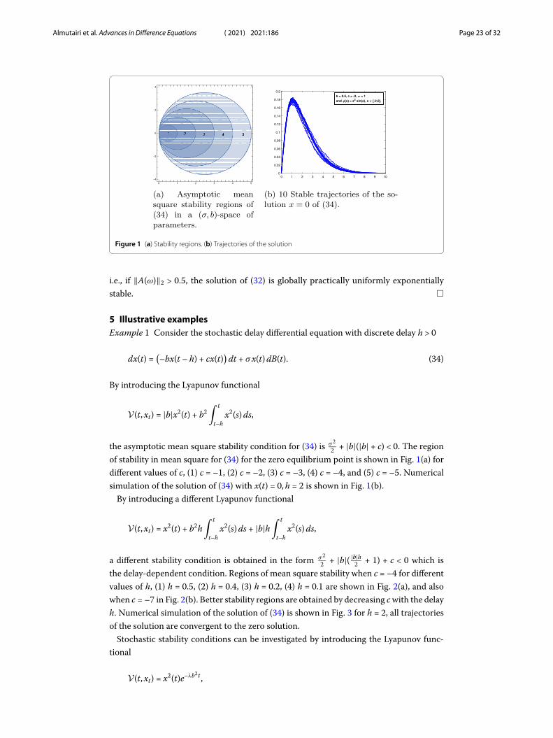
Figure 1 (a) Stability regions. (b) Trajectories of the solution

i.e., if ‖A(ω)‖2 > 0.5, the solution of (32) is globally practically uniformly exponentiallystable. �

5 Illustrative examplesExample 1 Consider the stochastic delay differential equation with discrete delay h > 0

dx(t) =(–bx(t – h) + cx(t)

)dt + σx(t) dB(t). (34)

By introducing the Lyapunov functional

V(t, xt) = |b|x2(t) + b2∫ t

t–hx2(s) ds,

the asymptotic mean square stability condition for (34) is σ 2

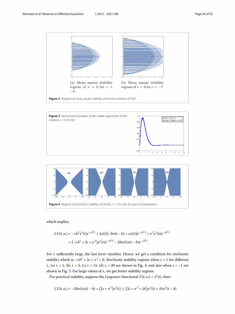
2 + |b|(|b| + c) < 0. The regionof stability in mean square for (34) for the zero equilibrium point is shown in Fig. 1(a) fordifferent values of c, (1) c = –1, (2) c = –2, (3) c = –3, (4) c = –4, and (5) c = –5. Numericalsimulation of the solution of (34) with x(t) = 0, h = 2 is shown in Fig. 1(b).

By introducing a different Lyapunov functional

V(t, xt) = x2(t) + b2h∫ t

t–hx2(s) ds + |b|h

∫ t

t–hx2(s) ds,

a different stability condition is obtained in the form σ 2

2 + |b|( |b|h2 + 1) + c < 0 which is

the delay-dependent condition. Regions of mean square stability when c = –4 for differentvalues of h, (1) h = 0.5, (2) h = 0.4, (3) h = 0.2, (4) h = 0.1 are shown in Fig. 2(a), and alsowhen c = –7 in Fig. 2(b). Better stability regions are obtained by decreasing c with the delayh. Numerical simulation of the solution of (34) is shown in Fig. 3 for h = 2, all trajectoriesof the solution are convergent to the zero solution.

Stochastic stability conditions can be investigated by introducing the Lyapunov func-tional

V(t, xt) = x2(t)e–λb2t ,

Almutairi et al. Advances in Difference Equations (2021) 2021:186 Page 24 of 32

Figure 2 Regions of mean square stability of the zero solution of (34)

Figure 3 Numerical simulation of ten stable trajectories of thesolution x = 0 of (34)

Figure 4 Regions of stochastic stability of (34) for c = 1 in a (σ ,b)-space of parameters

which implies

LV(t, xt) = –λb2x2(t)e–λb2t + 2x(t)(–bx(t – h) + cx(t)

)e–λb2t + σ 2x2(t)e–λb2t

=(–λb2 + 2c + σ 2)x2(t)e–λb2t – 2bx(t)x(t – h)e–λb2t .

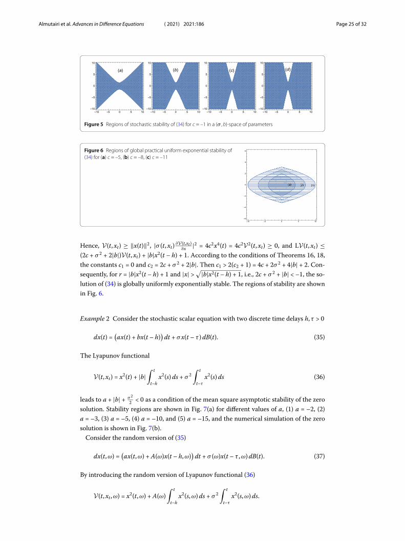
For λ sufficiently large, the last term vanishes. Hence, we get a condition for stochasticstability which is –λb2 + 2c + σ 2 < 0. Stochastic stability regions when c = 1 for differentλ, (a) λ = 1, (b) λ = 5, (c) λ = 15, (d) λ = 20 are shown in Fig. 4, and also when c = –1 areshown in Fig. 5. For large values of λ, we get better stability regions.

For practical stability, suppose the Lyapunov functional V(t, xt) = x2(t), then

LV(t, xt) = –2bx(t)x(t – h) +(2c + σ 2)x2(t) ≤ (

2c + σ 2 + |b|)x2(t) + |b|x2(t – h).

Almutairi et al. Advances in Difference Equations (2021) 2021:186 Page 25 of 32

Figure 5 Regions of stochastic stability of (34) for c = –1 in a (σ ,b)-space of parameters

Figure 6 Regions of global practical uniform exponential stability of(34) for (a) c = –5, (b) c = –8, (c) c = –11

Hence, V(t, xt) ≥ ‖x(t)‖2, |σ (t, xt) ∂V(t,xt )∂x |2 = 4c2x4(t) = 4c2V2(t, xt) ≥ 0, and LV(t, xt) ≤

(2c + σ 2 + 2|b|)V(t, xt) + |b|x2(t – h) + 1. According to the conditions of Theorems 16, 18,the constants c1 = 0 and c2 = 2c + σ 2 + 2|b|. Then c1 > 2(c2 + 1) = 4c + 2σ 2 + 4|b| + 2. Con-sequently, for r = |b|x2(t – h) + 1 and |x| >

√|b|x2(t – h) + 1, i.e., 2c + σ 2 + |b| < –1, the so-lution of (34) is globally uniformly exponentially stable. The regions of stability are shownin Fig. 6.

Example 2 Consider the stochastic scalar equation with two discrete time delays h, τ > 0

dx(t) =(ax(t) + bx(t – h)

)dt + σx(t – τ ) dB(t). (35)

The Lyapunov functional

V(t, xt) = x2(t) + |b|∫ t

t–hx2(s) ds + σ 2

∫ t

t–τ

x2(s) ds (36)

leads to a + |b| + σ 2

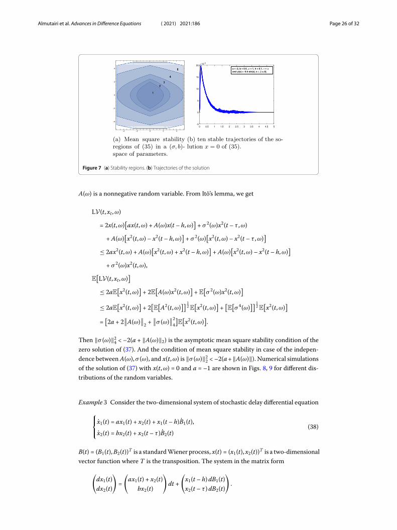
2 < 0 as a condition of the mean square asymptotic stability of the zerosolution. Stability regions are shown in Fig. 7(a) for different values of a, (1) a = –2, (2)a = –3, (3) a = –5, (4) a = –10, and (5) a = –15, and the numerical simulation of the zerosolution is shown in Fig. 7(b).

Consider the random version of (35)

dx(t,ω) =(ax(t,ω) + A(ω)x(t – h,ω)

)dt + σ (ω)x(t – τ ,ω) dB(t). (37)

By introducing the random version of Lyapunov functional (36)

V(t, xt ,ω) = x2(t,ω) + A(ω)∫ t

t–hx2(s,ω) ds + σ 2

∫ t

t–τ

x2(s,ω) ds.

Almutairi et al. Advances in Difference Equations (2021) 2021:186 Page 26 of 32

Figure 7 (a) Stability regions. (b) Trajectories of the solution

A(ω) is a nonnegative random variable. From Itô’s lemma, we get

LV(t, xt ,ω)

= 2x(t,ω)[ax(t,ω) + A(ω)x(t – h,ω)

]+ σ 2(ω)x2(t – τ ,ω)

+ A(ω)[x2(t,ω) – x2(t – h,ω)

]+ σ 2(ω)

[x2(t,ω) – x2(t – τ ,ω)

]

≤ 2ax2(t,ω) + A(ω)[x2(t,ω) + x2(t – h,ω)

]+ A(ω)

[x2(t,ω) – x2(t – h,ω)

]

+ σ 2(ω)x2(t,ω),

E[LV(t, xt ,ω)

]

≤ 2aE[x2(t,ω)

]+ 2E

[A(ω)x2(t,ω)

]+ E

[σ 2(ω)x2(t,ω)

]

≤ 2aE[x2(t,ω)

]+ 2

[E

[A2(t,ω)

]] 12 E

[x2(t,ω)

]+

[E

[σ 4(ω)

]] 12 E

[x2(t,ω)

]

=[2a + 2

∥∥A(ω)

∥∥

2 +∥∥σ (ω)

∥∥2

4

]E

[x2(t,ω)

].

Then ‖σ (ω)‖24 < –2(a + ‖A(ω)‖2) is the asymptotic mean square stability condition of the

zero solution of (37). And the condition of mean square stability in case of the indepen-dence between A(ω),σ (ω), and x(t,ω) is ‖σ (ω)‖2

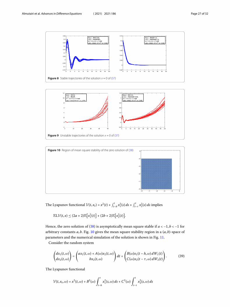
2 < –2(a +‖A(ω)‖). Numerical simulationsof the solution of (37) with x(t,ω) = 0 and a = –1 are shown in Figs. 8, 9 for different dis-tributions of the random variables.

Example 3 Consider the two-dimensional system of stochastic delay differential equation

⎧⎨

⎩x1(t) = ax1(t) + x2(t) + x1(t – h)B1(t),

x2(t) = bx2(t) + x2(t – τ )B2(t)(38)

B(t) = (B1(t), B2(t))T is a standard Wiener process, x(t) = (x1(t), x2(t))T is a two-dimensionalvector function where T is the transposition. The system in the matrix form

(dx1(t)dx2(t)

)

=

(ax1(t) + x2(t)

bx2(t)

)

dt +

(x1(t – h) dB1(t)x2(t – τ ) dB2(t)

)

.

Almutairi et al. Advances in Difference Equations (2021) 2021:186 Page 27 of 32

Figure 8 Stable trajectories of the solution x = 0 of (37)

Figure 9 Unstable trajectories of the solution x = 0 of (37)

Figure 10 Region of mean square stability of the zero solution of (38)

The Lyapunov functional V(t, xt) = x2(t) +∫ t

t–h x21(s) ds +

∫ tt–τ

x22(s) ds implies

ELV(t, x) ≤ (2a + 2)E[x2

1(t)]

+ (2b + 2)E[x2

2(t)].

Hence, the zero solution of (38) is asymptotically mean square stable if a < –1, b < –1 forarbitrary constants a, b. Fig. 10 gives the mean square stability region in a (a, b)-space ofparameters and the numerical simulation of the solution is shown in Fig. 11.

Consider the random system

(dx1(t,ω)dx2(t,ω)

)

=

(ax1(t,ω) + A(ω)x2(t,ω)

bx2(t,ω)

)

dt +

(B(ω)x1(t – h,ω) dW1(t)C(ω)x2(t – τ ,ω) dW2(t)

)

. (39)

The Lyapunov functional

V(t, xt ,ω) = x2(t,ω) + B2(ω)∫ t

t–hx2

1(s,ω) ds + C2(ω)∫ t

t–τ

x22(s,ω) ds

Almutairi et al. Advances in Difference Equations (2021) 2021:186 Page 28 of 32

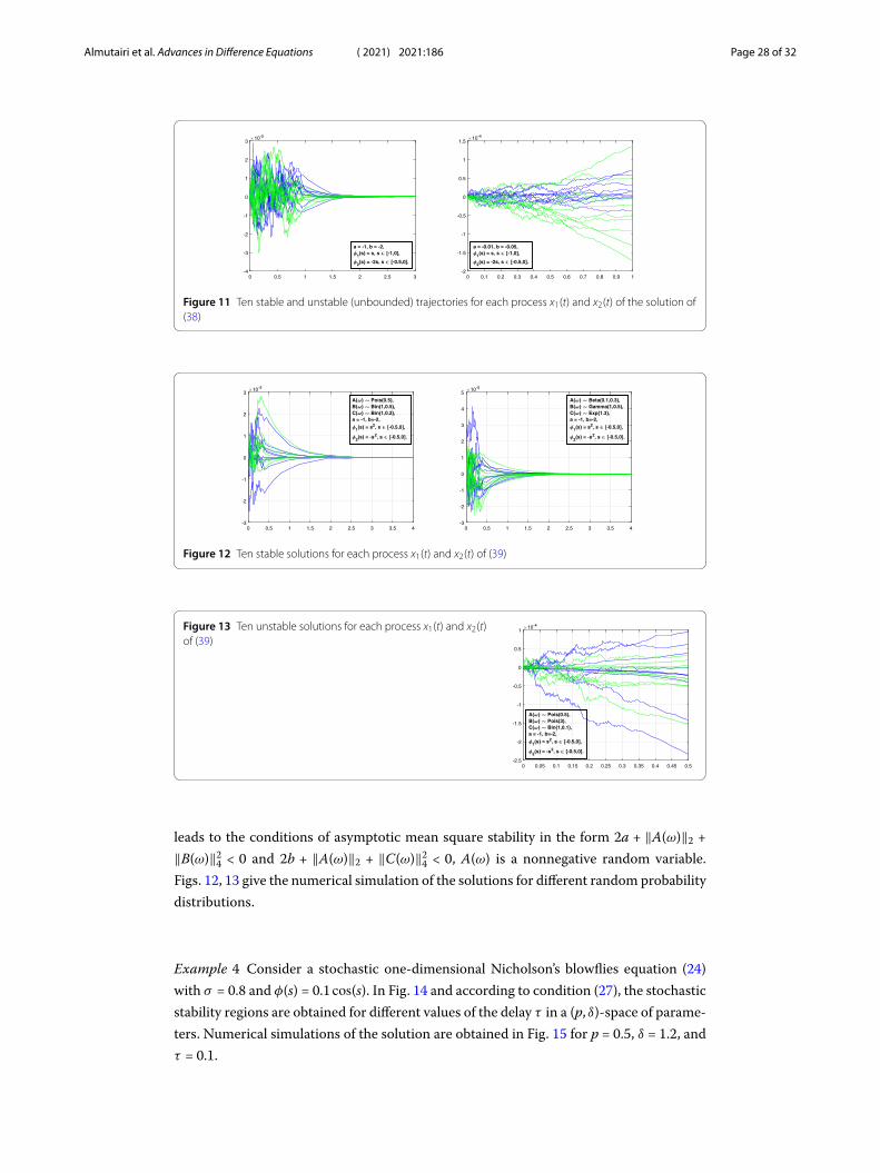
Figure 11 Ten stable and unstable (unbounded) trajectories for each process x1(t) and x2(t) of the solution of(38)

Figure 12 Ten stable solutions for each process x1(t) and x2(t) of (39)

Figure 13 Ten unstable solutions for each process x1(t) and x2(t)of (39)

leads to the conditions of asymptotic mean square stability in the form 2a + ‖A(ω)‖2 +‖B(ω)‖2

4 < 0 and 2b + ‖A(ω)‖2 + ‖C(ω)‖24 < 0, A(ω) is a nonnegative random variable.

Figs. 12, 13 give the numerical simulation of the solutions for different random probabilitydistributions.

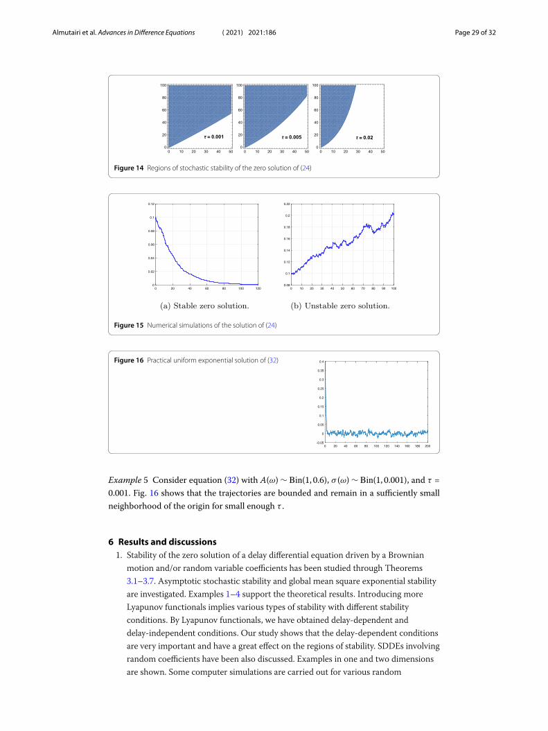
Example 4 Consider a stochastic one-dimensional Nicholson’s blowflies equation (24)with σ = 0.8 and φ(s) = 0.1 cos(s). In Fig. 14 and according to condition (27), the stochasticstability regions are obtained for different values of the delay τ in a (p, δ)-space of parame-ters. Numerical simulations of the solution are obtained in Fig. 15 for p = 0.5, δ = 1.2, andτ = 0.1.

Almutairi et al. Advances in Difference Equations (2021) 2021:186 Page 29 of 32

Figure 14 Regions of stochastic stability of the zero solution of (24)

Figure 15 Numerical simulations of the solution of (24)

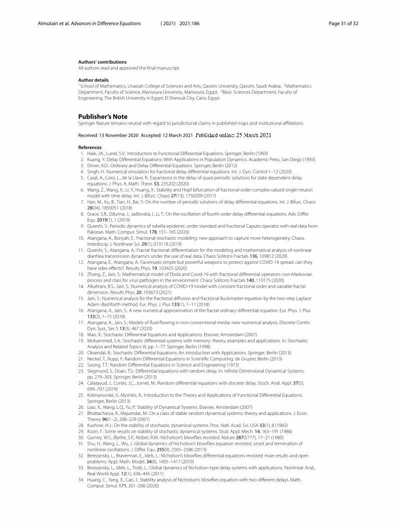
Figure 16 Practical uniform exponential solution of (32)

Example 5 Consider equation (32) with A(ω) ∼ Bin(1, 0.6), σ (ω) ∼ Bin(1, 0.001), and τ =0.001. Fig. 16 shows that the trajectories are bounded and remain in a sufficiently smallneighborhood of the origin for small enough τ .

6 Results and discussions1. Stability of the zero solution of a delay differential equation driven by a Brownian

motion and/or random variable coefficients has been studied through Theorems3.1–3.7. Asymptotic stochastic stability and global mean square exponential stabilityare investigated. Examples 1–4 support the theoretical results. Introducing moreLyapunov functionals implies various types of stability with different stabilityconditions. By Lyapunov functionals, we have obtained delay-dependent anddelay-independent conditions. Our study shows that the delay-dependent conditionsare very important and have a great effect on the regions of stability. SDDEs involvingrandom coefficients have been also discussed. Examples in one and two dimensionsare shown. Some computer simulations are carried out for various random

Almutairi et al. Advances in Difference Equations (2021) 2021:186 Page 30 of 32

probability distributions. These random variables provide various patterns to thesolution stochastic process and make the model more attractive. The mainapplication in this paper is Nicholson’s blowflies model. Propositions 4.1, 4.2 havestudied the stochastic stability and stochastic global exponential stability for the zerosolution, respectively. Regions of stability of the zero solution at which these blowfliesbecome extinct are shown. These regions become better for small values of delay τ .Regarding the financial market application, Proposition 4.3 has studied the stabilityof a stochastic Black–Scholes model with random variable coefficients.

2. Theorems 3.8, 3.9 have studied the practical stability of the solution when the originis not necessarily an equilibrium point. By these theorems, we have concluded that alltrajectories of the solution of the Black–Scholes model are practically uniformlyexponentially stable. According to Example 5, for small enough τ and ‖A(ω)‖2 ≥ 1

2 ,almost all trajectories are bounded and remain in a sufficiently small neighborhoodof the origin.

By stochastic mathematical epidemiological and ecological models, we can reveal themechanisms that influence the transmission and control the disease. Stochastic modelsare proposed to capture the uncertainty and variations in the transmission of the diseases.Many recent works dedicated to stochastic epidemiological and ecological models can befound in [37, 38, 40, 41, 50, 52, 58–61]. There is still considerable uncertainty with regardto the study of stability, therefore we have addressed the stochastic global exponentialand practical stability. Mathematically, we have focused on the qualitative theory (stabil-ity of equilibria) of stochastic/random systems in a rigorous way. From ecological point ofview, dynamics of stochastic Nicholson’s blowflies models is studied. We claim that ourapproach can be extended to various biological, ecological, and economical models. Thisapproach will reveal some important aspects of these models.

7 Conclusion and further directionsIn this paper, we have studied the stability of Nicholson’s blowflies model and Black–Scholes market model based on some important proven theorems in asymptotic stochas-tic stability, global exponential mean square stability, and practical uniform exponentialstability. Our results on Nicholson’s blowflies model can be extended to its general formknown as the stochastic neoclassical growth model, for γ > 0,γ �= 1

dx(t) =(pxγ (t – τ )e–ax(t–τ ) – δx(t)

)dt + σx(t) dB(t).

Moreover, we hope that our findings will be useful for models driven by fractional Brow-nian motion (FBM).

AcknowledgementsNot applicable.

FundingThis work was supported by the Mathematics Department - Mansoura University of Egypt.

Availability of data and materialsThe data sets generated and/or analyzed during the current study are available from the corresponding author onreasonable request.

Competing interestsThe authors declare that they have no competing interests.

Almutairi et al. Advances in Difference Equations (2021) 2021:186 Page 31 of 32

Authors’ contributionsAll authors read and approved the final manuscript.

Author details1School of Mathematics, Unaizah College of Sciences and Arts, Qassim University, Qassim, Saudi Arabia. 2MathematicsDepartment, Faculty of Science, Mansoura University, Mansoura, Egypt. 3Basic Sciences Department, Faculty ofEngineering, The British University in Egypt, El Sherouk City, Cairo, Egypt.

Publisher’s NoteSpringer Nature remains neutral with regard to jurisdictional claims in published maps and institutional affiliations.

Received: 13 November 2020 Accepted: 12 March 2021

References1. Hale, J.K., Lunel, S.V.: Introduction to Functional Differential Equations. Springer, Berlin (1993)2. Kuang, Y.: Delay Differential Equations: With Applications in Population Dynamics. Academic Press, San Diego (1993)3. Driver, R.D.: Ordinary and Delay Differential Equations. Springer, Berlin (2012)4. Singh, H.: Numerical simulation for fractional delay differential equations. Int. J. Dyn. Control 1–12 (2020)5. Casal, A., Corsi, L., de la Llave, R.: Expansions in the delay of quasi-periodic solutions for state dependent delay

equations. J. Phys. A, Math. Theor. 53, 235202 (2020)6. Wang, Z., Wang, X., Li, Y., Huang, X.: Stability and Hopf bifurcation of fractional-order complex-valued single neuron

model with time delay. Int. J. Bifurc. Chaos 27(13), 1750209 (2017)7. Han, M., Xu, B., Tian, H., Bai, Y.: On the number of periodic solutions of delay differential equations. Int. J. Bifurc. Chaos

28(04), 1850051 (2018)8. Grace, S.R., Džurina, J., Jadlovská, I., Li, T.: On the oscillation of fourth-order delay differential equations. Adv. Differ.

Equ. 2019(1), 1 (2019)9. Qureshi, S.: Periodic dynamics of rubella epidemic under standard and fractional Caputo operator with real data from

Pakistan. Math. Comput. Simul. 178, 151–165 (2020)10. Atangana, A., Bonyah, E.: Fractional stochastic modeling: new approach to capture more heterogeneity. Chaos,

Interdiscip. J. Nonlinear Sci. 29(1), 013118 (2019)11. Qureshi, S., Atangana, A.: Fractal-fractional differentiation for the modeling and mathematical analysis of nonlinear

diarrhea transmission dynamics under the use of real data. Chaos Solitons Fractals 136, 109812 (2020)12. Atangana, E., Atangana, A.: Facemasks simple but powerful weapons to protect against COVID-19 spread: can they

have sides effects?. Results Phys. 19, 103425 (2020)13. Zhang, Z., Jain, S.: Mathematical model of Ebola and Covid-19 with fractional differential operators: non-Markovian

process and class for virus pathogen in the environment. Chaos Solitons Fractals 140, 110175 (2020)14. Alkahtani, B.S., Jain, S.: Numerical analysis of COVID-19 model with constant fractional order and variable fractal

dimension. Results Phys. 20, 103673 (2021)15. Jain, S.: Numerical analysis for the fractional diffusion and fractional Buckmaster equation by the two-step Laplace

Adam–Bashforth method. Eur. Phys. J. Plus 133(1), 1–11 (2018)16. Atangana, A., Jain, S.: A new numerical approximation of the fractal ordinary differential equation. Eur. Phys. J. Plus

133(2), 1–15 (2018)17. Atangana, A., Jain, S.: Models of fluid flowing in non-conventional media: new numerical analysis. Discrete Contin.

Dyn. Syst., Ser. S 13(3), 467 (2020)18. Mao, X.: Stochastic Differential Equations and Applications. Elsevier, Amsterdam (2007)19. Mohammed, S.A.: Stochastic differential systems with memory: theory, examples and applications. In: Stochastic

Analysis and Related Topics VI, pp. 1–77. Springer, Berlin (1998)20. Oksendal, B.: Stochastic Differential Equations: An Introduction with Applications. Springer, Berlin (2013)21. Neckel, T., Rupp, F.: Random Differential Equations in Scientific Computing. de Gruyter, Berlin (2013)22. Soong, T.T.: Random Differential Equations in Science and Engineering (1973)23. Siegmund, S., Doan, T.S.: Differential equations with random delay. In: Infinite Dimensional Dynamical Systems,

pp. 279–303. Springer, Berlin (2013)24. Calatayud, J., Cortés, J.C., Jornet, M.: Random differential equations with discrete delay. Stoch. Anal. Appl. 37(5),

699–707 (2019)25. Kolmanovskii, V., Myshkis, A.: Introduction to the Theory and Applications of Functional Differential Equations.

Springer, Berlin (2013)26. Liao, X., Wang, L.Q., Yu, P.: Stability of Dynamical Systems. Elsevier, Amsterdam (2007)27. Bhattacharya, R., Majumdar, M.: On a class of stable random dynamical systems: theory and applications. J. Econ.

Theory 96(1–2), 208–229 (2001)28. Kushner, H.J.: On the stability of stochastic dynamical systems. Proc. Natl. Acad. Sci. USA 53(1), 8 (1965)29. Kozin, F.: Some results on stability of stochastic dynamical systems. Stud. Appl. Mech. 14, 163–191 (1986)30. Gurney, W.S., Blythe, S.P., Nisbet, R.M.: Nicholson’s blowflies revisited. Nature 287(5777), 17–21 (1980)31. Shu, H., Wang, L., Wu, J.: Global dynamics of Nicholson’s blowflies equation revisited, onset and termination of

nonlinear oscillations. J. Differ. Equ. 255(9), 2565–2586 (2013)32. Berezansky, L., Braverman, E., Idels, L.: Nicholson’s blowflies differential equations revisited: main results and open

problems. Appl. Math. Model. 34(6), 1405–1417 (2010)33. Berezansky, L., Idels, L., Troib, L.: Global dynamics of Nicholson-type delay systems with applications. Nonlinear Anal.,

Real World Appl. 12(1), 436–445 (2011)34. Huang, C., Yang, X., Cao, J.: Stability analysis of Nicholson’s blowflies equation with two different delays. Math.

Comput. Simul. 171, 201–206 (2020)

Almutairi et al. Advances in Difference Equations (2021) 2021:186 Page 32 of 32

35. Wang, W., Wang, L., Chen, W.: Existence and exponential stability of positive almost periodic solution forNicholson-type delay systems. Nonlinear Anal., Real World Appl. 12(4), 1938–1949 (2011)

36. Hien, L.V.: Global asymptotic behaviour of positive solutions to a non-autonomous Nicholson’s blowflies model withdelays. J. Biol. Dyn. 8(1), 135–144 (2014)

37. Wang, W., Shi, C., Chen, W.: Stochastic Nicholson-type delay differential system. Int. J. Control 1–8 (2019)38. Wang, W., Wang, L., Chen, W.: Stochastic Nicholson’s blowflies delayed differential equations. Appl. Math. Lett. 87,

20–26 (2019)39. Black, F., Scholes, M.: The pricing of options and corporate liabilities. J. Polit. Econ. 81(3), 637–654 (1973)40. Ghysels, E., Harvey, A.C., Renault, E.: Stochastic volatility. Handb. Stat. 14, 119–191 (1996)41. Ekström, E., Tysk, J.: The Black–Scholes equation in stochastic volatility models. J. Math. Anal. Appl. 368(2), 498–507

(2010)42. Ricciardi, L.M., Sacerdote, L.: The Ornstein–Uhlenbeck process as a model for neuronal activity. Biol. Cybern. 35(1), 1–9

(1979)43. Zeng, C., Chen, Y., Yang, Q.: Almost sure and moment stability properties of fractional order Black–Scholes model.

Fract. Calc. Appl. Anal. 16(2), 317–331 (2013)44. Maruyama, G.: Continuous Markov processes and stochastic equations. Rend. Circ. Mat. Palermo 4(1), 1–48 (1955)45. Bokil, V.A., Gibson, N.L., Nguyen, S.L., Thomann, E.A., Waymire, E.C.: An Euler–Maruyama method for diffusion

equations with discontinuous coefficients and a family of interface conditions. J. Comput. Appl. Math. 368, 112545(2020)

46. Milshtein, G.N.: Teor. Veroâtn. Primen. (in Russian) 19(3), (1974)47. Sohaly, M.A., Yassen, M.T., Elbaz, I.M.: Stochastic consistency and stochastic stability in mean square sense for Cauchy

advection problem. J. Differ. Equ. Appl. 24(1), 59–67 (2018)48. Yassen, M.T., Sohaly, M.A., Random, E.I.M.: Crank–Nicolson scheme for random heat equation in mean square sense.

Am. J. Comput. Math. 6(2), 66–73 (2016)49. Yassen, M.T., Sohaly, M.A., Elbaz, I.M.: Stochastic solution for Cauchy one-dimensional advection model in mean

square calculus. J. Assoc. Arab Univ. Basic Appl. Sci. 24, 263–270 (2017)50. El-Metwally, H., Sohaly, M.A., Elbaz, I.M.: Stochastic global exponential stability of disease-free equilibrium of HIV/AIDS

model. Eur. Phys. J. Plus 135(10), 1–14 (2020)51. Mao, X.: Exponential Stability of Stochastic Differential Equations. Dekker, New York (1994)52. Khasminskii, R.: Stochastic Stability of Differential Equations. Springer, Berlin (2011)53. Villafuerte, R., Mondié, S., Poznyak, A.: Practical stability of time delay systems: LMI’s approach. In: 2008 47th IEEE

Conference on Decision and Control, pp. 4807–4812. IEEE Press, New York (2008)54. La Salle, J., Lefschetz, S.: Stability by Lyapunov’s Direct Method with Applications. Academic Press, London (1961)55. Lakshmikantham, V., Leela, S., Martynyuk, A.: Practical Stability of Nonlinear Systems. World Scientific, Singapore

(1990)56. Friz, P., Victoir, N.: The Burkholder–Davis–Gundy inequality for enhanced martingales. In: Séminaire de Probabilités

XLI, pp. 421–438. Springer, Berlin (2008)57. Chandra, T.K.: The Borel–Cantelli Lemma. Springer, Berlin (2012)58. Gray, A., Greenhalgh, D., Hu, L., Mao, X., Pan, J.: A stochastic differential equation SIS epidemic model. SIAM J. Appl.

Math. 71(3), 876–902 (2011)59. Cai, S., Cai, Y., Mao, X.: A stochastic differential equation SIS epidemic model with two independent Brownian

motions. J. Math. Anal. Appl. 474(2), 1536–1550 (2019)60. Britton, T.: Stochastic epidemic models: a survey. Math. Biosci. 225(1), 24–35 (2010)61. Schurz, H., Tosun, K.: Stability of stochastic SIS model with disease deaths and variable diffusion rates. Electron. J. Qual.

Theory Differ. Equ. 2019 14, (2019)