Lyapunov Exponents versus Expansivity and Sensitivity in Cellular Automata

File: DISTL2 047401 . By:CV . Date:29:05:98 . Time:10:58 LOP8M. V8.B. Page 01:01Codes: 3974 Signs: 1894 . Length: 45 pic 0 pts, 190 mm

journal of complexity 14, 210�233 (1998)

Lyapunov Exponents versus Expansivity andSensitivity in Cellular Automata*

Michele Finelli

Dipartimento di Matematica, Universita� di Siena,Via del Capitano 15, I-53100 Siena, Italy

E-mail: finelli�cs.unibo.it

Giovanni Manzini

Dipartimento di Scienze e Tecnologie Avanzate, Via Cavour 84, I-15100 Alessandria, Italy,and Instituto di Matematica Computazionale, CNR, Via S. Maria 46, I-56126 Pisa, Italy

E-mail: manzini�mfn.al.unipmn.it

and

Luciano Margara

Dipartimento di Scienze dell 'Informazione, Universita� di Bologna,Mura Anteo Zamboni 7, I-40127 Bologna, Italy

E-mail: margara�cs.unibo.it

Received November 11, 1996

We establish a connection between the theory of Lyapunov exponents and theproperties of expansivity and sensitivity to initial conditions for a particular classof discrete time dynamical systems; cellular automata (CA). The main contributionof this paper is the proof that all expansive cellular automata have positiveLyapunov exponents for almost all the phase space configurations. In addition, weprovide an elementary proof of the non-existence of expansive CA in any dimensiongreater than 1. In the second part of this paper we prove that expansivity in dimen-sion greater than 1 can be recovered by restricting the phase space to a suitable sub-set of the whole space. To this extent we describe a 2-dimensional CA which isexpansive over a dense uncountable subset of the whole phase space. Finally, wehighlight the different behavior of expansive and sensitive CA for what concerns thespeed at which perturbations propagate. � 1998 Academic Press

article no. CM980474

2100885-064X�98 �25.00Copyright � 1998 by Academic PressAll rights of reproduction in any form reserved.

* A preliminary version of this paper appeared in the Proceedings of the 2nd Conferenceon Cellular Automata for Research and Industry (ACRI'96), Milan, Italy, 1996.


1. INTRODUCTION

The notion of chaos is very appealing, and it has intrigued many scien-tists (see [2, 3, 14, 17, 20] for some works on the properties that charac-terize a chaotic process). In the case of discrete time dynamical systems(DTDS) defined on a metric space, many definitions of chaos are based onthe notion of sensitivity (see for example [8, 13, 17]). We now recall thedefinition of sensitivity to initial conditions for a generic DTDS (X, F ).Here, we assume that X is equipped with a distance d and that the mapF : X � X is continuous on X according to the metric topology inducedby d.

Definition 1 (Sensitivity). A DTDS (X, F ) is sensitive to initial condi-tions if and only if there exists $>0 such that

\x # X \=>0 _y # X _n�0: d(x, y)<= and d(F n(x), F n( y))>$.

The value $ is called the sensitivity constant.

Intuitively, a map is sensitive to initial conditions, or simply sensitive, ifthere exist points arbitrarily close to x which eventually separate from x byat least $ under iteration of F. We emphasize that not all points near xneed eventually separate from x, but there must be at least one such pointin every neighborhood of x. If a map is sensitive to initial conditions, then,for all practical purposes, the dynamics of the map defies numericalapproximation. Small errors in computation which are introduced byround-off may become magnified upon iteration. The results of numericalcomputation of an orbit, no matter how accurate, may be completelydifferent from the real orbit.

A property stronger than sensitivity is expansivity. Expansivity differsfrom sensitivity in that all nearby points eventually separate by at least $.It is easy to verify that expansive CA are sensitive to initial conditions.

Definition 2 (Expansivity). A DTDS (X, F ) is expansive if and only ifthere exists $>0 such that

\x, y # X x{ y _n�0: d(F n(x), F n( y))>$.

The value $ is called the expansivity constant.

Sometimes the definition of expansivity given above is referred to asforward or positive expansivity in order to distinguish it from the notion ofexpansivity given for invertible (one-to-one) dynamical systems where``_n�0'' is replaced by ``_n # Z.''

211LYAPUNOV EXPONENTS


In the case of differentiable spaces there is another parameter which isoften used for detecting chaotic behaviors: Lyapunov exponents. We definethem for a map F : I � I, where I is a real interval.

Definition 3 (Lyapunov Exponents). Let (I, F ) be a DTDS. TheLyapunov exponent *(x) of x # X is defined by

*(x)= limn � �

1n

log \dF n(x)dx + .

Lyapunov exponents can be easily generalized to higher dimensions.Usually, a DTDS (I, F ) is said to be chaotic at x # X if and only if *(x)>0.

In this paper we wish to discuss the role played by time in the definitionsof expansivity, sensitivity and Lyapunov exponents. According toDefinition 2, a DTDS (X, F ) is said to be expansive if and only if after anunspecified number of applications of F, every pair of configurations, nomatter how close they are, are separated by a preassigned constant value $.The same consideration can be done for a sensitive DTDS. (X, F ) is expan-sive even if the number of iterations needed for separating is of the orderof 10100. In other words, a quantitative measure of time does not come intoplay in determining the expansivity of a DTDS. This is one of the maincriticisms made by those who prefer a Lyapunov exponent based approachfor defining chaos.

Time plays a fundamental role in the definition of Lyapunov exponents.In fact, if *(x)>0, we have

dF n(x)dx

&:n*(x),

where :>1. This means that F at x shows an exponential rate divergencein time. Unfortunately, Lyapunov exponents have many other drawbacks.The main one is that in many cases they cannot be computed in a closeform and one needs to approximate them by time consuming and, some-times, unreliable computer simulations (as in the case of CA).

In this paper we prove that, for cellular automata, the criticisms made bythe supporters of the Lyapunov exponents to the expansivity property arenot well founded. In fact, we show that every expansive CA must havealmost all Lyapunov exponents uniformly bounded away from zero by aconstant $ which only depends on the CA we consider. In other words,expansivity implies positive Lyapunov exponents. Note that the task ofverifying expansivity appears to be simpler than the computation of theLyapunov exponents. In [9], the authors define a large class of expansiveCA which contains additive and non-additive ones, while in [16] the class

212 FINELLI, MANZINI, AND MARGARA


of expansive additive CA is characterized in terms of a simple property ofthe coefficients of the local rule.

The main results of this paper can be summarized as follows.

1. Let (X, F ) be any expansive CA with expansivity constant $. Letx, y # X be any pair of distinct configurations whose distance is =. Thenumber of iterations needed by F for separating x and y by at least $depends only on = and is of the order of log($�=) (Corollary 4.5). Inaddition, we show that a similar result does not hold for sensitive CA(Example 3).

2. Every expansive CA (X, F ) has positive (uniformly bounded awayfrom zero) Lyapunov exponents over a set Y�X of configurations of fullmeasure. A slightly weaker result holds also for those configurationsbelonging to X"Y (Theorem 5.2).

3. We provide an elementary proof of the non existence of D-dimen-sional CA for D�2 (Theorem 4.4). A (much more complex) proof of thisresult has been given by Shereshevsky [19, Corollary 2] in the moregeneral setting of group actions by endomorphisms. We also show thatexpansivity can be achieved in dimension greater than 1 if we restrict our-selves to a suitable subset of the phase space. More precisely, we show thatthere exists a 2-dimensional CA (X, F ) which is expansive on a denseinvariant subset of X (Theorem 6.3).

The rest of this paper is organized as follows. In Section 2 we give basicdefinitions and notations. In Section 3 we review the notion of Lyapunovexponents for CA and we recall some known results concerning CA andLyapunov exponents. In Section 4 we prove the main results on expansiveCA and we highlight some differences among expansive CA and generalexpansive maps. In Section 5 we show the relationship between expansivityand Lyapunov exponents in CA. In Section 6 we prove the existence of CAwhich are expansive over a dense subset of the whole space but are notglobally expansive. In Section 7 we compare the behavior of expansive andsensitive CA for what concerns the number of iterations required toseparate neighboring configurations. Section 8 contains some concludingremarks.

2. DEFINITIONS AND NOTATIONS

Let A=[0, 1, ..., p&1] be a finite alphabet of cardinality p�2. Weconsider the space of configurations

AZD=[c | c : ZD � A],



which consists of all functions from ZD into A. For example, each elementof AZ2

can be visualized as an infinite 2-dimensional lattice in which eachcell contains an element of A.

Let s�1. A neighborhood frame of size s is an ordered set of distinctvector u� 1 , u� 2 , ..., u� s # ZD. Given f : As � A, a D-dimensional CA based onthe local rule f is the pair (AZD

, F ), where F : AZD� AZD

, is the globaltransition map defined as follows. For every c # AZD

the configuration F(c)is such that for every v� # ZD,

[F(c)](v� )= f (c(v� +u� 1), ..., c(v� +u� s)).

In other words, the content of cell v� in the configuration F(c) is a functionof the content of cells v� +u� 1 , ..., v� +u� s in the configuration c. Note that thelocal rule f and the neighborhood frame completely determine F.

Example 1. When s=1 and f is the identity map, we have

[F(c)](v� )=c(v� +u� 1).

Hence, the global transition map F is simply a shift of the configurationspace AZD

. In this case, we say that F is a shift map and we denote itby _u� 1. A fundamental property of the shift maps is that they commutewith the global map of any other CA. That is, for any u� # ZD and c # AZD

,we have _u� (F(c))=F(_u� (c)).

For 1-dimensional CA, we use a simplified notation. Let f : A2k+1 � A,be any map. A 1-dimensional CA based on the local rule f is a pair(AZ, F ), where F : AZ � AZ, is defined by

[F(c)](i)= f (c(i&k), ..., c(i+k)), c # AZ, i # Z.

We say that k is the radius of f. Note that, even if f (x&k , ..., x&1 , x0 ,x1 , ..., xk) must depend on at least one between x&k and xk , in general fdoes not depend on all the 2k+1 variables x&k , ..., xk .

Example 2. An important 1-dimensional CA is the right shift map(AZ, _) defined by

[_(c)](i)=c(i&1).

The global map _ corresponds to the local rule f (x&1 , x0 , x1)=x&1 . Theinverse of _ is the left shift map defined by [_&1(c)](i)=c(i+1) which



corresponds to the local rule f (x&1 , x0 , x1)=x1 . For j�0 the iterated map_ j is such that

[_ j (c)](i)=c(i& j), c # AZ, i # Z. (1)

In the following we use _ j with j<0 to denote the map _&1 iterated | j |times. Note that, using this notation, (1) holds for any j # Z.

In order to specialize the notions of sensitivity and expansitivity to thecase of D-dimensional CA, we need to introduce a distance mapping overthe space AZD

. In the literature there are many examples of distance map-pings over AZD

(see for example [4, 5, 10, 11, 15]). Most of them induceover AZD

the so-called product topology.1 With this topology, AZDis a

compact and totally disconnected space and every CA is a uniformly con-tinuous map.

Among all the distances over AZDthat induce the product topology we

use the following one which enables us to prove our results in the simplestway. Given x, y # AZD

such that x{ y we define

(x, y) �=min[&v� &� | v� # ZD and x(v� ){ y(v� )],

where &v� &� is the maximum of the absolute value of the components of v� .Define

d(x, y)={0,2&(x, y)�,

if x= y,if x{ y.

(2)

The distance d has been used for example in [4, 15].Throughout the paper, F(c) will denote the result of the application of

the map F to the configuration c, and c(v� ) will denote the value of theentry with coordinates v� of the configuration c. We recursively define F n(c)by F n(c)=F(F n&1(c)), where F 0(c)=c.

3. LYAPUNOV EXPONENTS FOR CA

The notion of Lyapunov exponents given in Definition 3 can be appliedonly to differentiable spaces. Since AZ is not a differentiable space, for CAwe need an ad hoc definition. In this section we recall the definition of


1 The product topology over AZDis that induced by the discrete topology on A.


Lyapunov exponents for the special case of 1-dimensional CA given in[18]. There, the authors introduce quantities analogous to Lyapunovexponents of smooth dynamical systems with the aim of describing thelocal instability of orbits in CA.

For every x # AZ and s�0 we set

W &s (x)=[ y # AZ : y(i)=x(i) for all i�&s],

W +s (x)=[ y # AZ : y(i)=x(i) for all i�s].

We have that W +i (x)/W +

i+1(x) and W &i (x)/W &

i+1(x). For every n�0we define

4� &n (x)=min[s�0: F n(W &

0 (x))/W &s (F n(x))],

4� +n (x)=min[s�0: F n(W +

0 (x))/W +s (F n(x))].

Intuitively, for the CA defined by F the value 4� +n (x) [4� &

n (x)] measureshow far a perturbation front moves right [left] in time n if the front isinitially located at i=0. Finally, we consider the shift invariant quantities

4&n (x)=max

j # Z4� &

n (_ j (x)), 4+n (x)=max

j # Z4� +

n (_ j (x)),

where _ denotes the right shift map defined in Example 2. Intuitively, thevalue 4� +

n (_ j (x)) [4� &n (_ j (n))] measures how far a perturbation front

moves right [left] in time n if the front is initially located at j.The values *+(x) and *&(x) defined by

*+(x)= limn � �

1n

4+n (x) *&(x)= lim

n � �

1n

4&n (x) (3)

are called respectively the right and left Lyapunov exponents of the CA Ffor the configuration x. The limits in (3) do not necessarily exist for allx # AZ. However, the following result holds.

Theorem 3.1 [18]. For any _-invariant and F-invariant measure +defined on AZ, there exists a set Y�X of full measure (+(Y)=1) such thatfor every x # Y the limits (3) exist.

Typical examples of _-invariant and F-invariant measures are theso-called Bernoulli product measures (see [7] for details).



4. SOME PROPERTIES OF EXPANSIVE CELLULAR AUTOMATA

In this section we study the properties of expansive functions over acompact metric space. In particular, we consider the case in which we aregiven a function F : X � X such that

_*>0: \x, y # X, d(F(x), F( y))�*d(x, y). (4)

Using calculus terminology, if (4) holds we say that F is a Lipschitz func-tion with parameter *. The reason for which we are interested in Lipschitzfunctions is that the global transition map F associated to a CA alwayssatisfies (4). In this case, the parameter * can be easily obtained from theradius of the local rule.

For any pair x, y # X, by (4) we have d(F n(x), F n( y))�*nd(x, y). hence,the distance d(F n(x), F n( y)) cannot grow arbitrarily fast. Our main interestis to get lower bounds on how fast this distance can grow for expansivemaps. Our main purpose is to prove some properties of expansive CAwhich will be used in the following sections. However, in doing so we willalso highlight the different behaviors of expansive CA with respect togeneral expansive Lipschitz functions.

Lemma 4.1. Let (X, d ) be a compact metric space, and F : X � X be anexpansive Lipschitz function. Then, we can find =$>0 such that for all =,0<=<=$, there exists n=n(=) such that

\x, y # X =�d(x, y)�=$ O _k�n : d(F k(x), F k( y))>2d(x, y). (5)

Proof. Assume F is expansive with parameter $, and let * denote theLipschitz constant of the function F. Note that we must have *>1otherwise F cannot be expansive. We prove the theorem for =$=$�6. Let=<=$. Assume by contradiction that

\n _xn , yn : =�d(xn , yn)�=$ and

d(F k(xn), F k( yn))�2d(xn , yn) \k�n.

Since X is a compact space, we can build two sequences xi , yi such that

=�d(xi , yi)�=$, limi � �

xi=x~ , limi � �

yi= y~ , (6)

and

d(F k(x i), F k( yi))�2d(xi , y i) \k�i. (7)



Moreover, we can assume that

d(xi , x~ )<$3

*&i, d( yi , y~ )<$3

*&i. (8)

By the triangle inequality, we have for all i,

d(x~ , y~ )�d(xi , yi)&d(x~ , xi)&d( yi , y~ )�=&2$3

*&i,

which implies x~ { y~ . For the expansivity of F there exists m such thatd(F m(x~ ), F m( y~ ))>$. Using again the triangle inequality, together with (8),we get

d(F m(xm), F m( ym))

�d(F m(x~ ), F m( y~ ))&d(F m(x~ ), F m(xm))&d(F m( y~ ), F m( ym))

>$&*md(x~ , xm)&*md( y~ , ym)

>$&$3

&$3

=$3

.

Since =$�$�6, we have

d(F m(xm), F m( ym))>2=$�2d(xm , ym),

which is impossible since it contradicts the hypothesis (7). K

Note that the above lemma can be applied several times to prove that wecan have an arbitrarily large growth of the initial distance. More precisely,let =$ and n(=) be given as in Lemma 4.1. Then, for any integer t>0 and=�=$2&t, we have

=�d(x, y)�=$2t O _k�(t+1) n(=) : d(F k(x), F k( y))>2t+1d(x, y). (9)

It is straightforward to verify that any map which satisfies (5) is expan-sive with parameter =$. Next theorem establishes that it suffices that (5)



holds on a dense subset of X to guarantee that F is expansive over thewhole space.

Theorem 4.2. let (X, d ) be a compact metric space, and F : X � X be aLipschitz function. Let Y be any dense subset of X such that F(Y )�Y. Ifthere exists =$ such that for all =<=$ we can find n=n(=) such that

\x, y # Y, =�d(x, y)�=$ O _k�n : d(F k(x), F k( y))�2d(x, y),

(10)

then F is expansive over X.

Proof. We prove that F is expansive with parameter =$�3 by showingthat

\x, y # X, x{ y, d(x, y)�=$�4 O _k : d(F k(x), F k( y))>=$�3.

Let x, y # X with d(x, y)�=$�4, and let n=n(d(x, y)�2). Since Y is a densesubset, we can find x~ , y~ # Y such that

d(x, x~ )�d(x, y)�4, d( y, y~ )�d(x, y)�4, (11)

and

*nWlog2(2=$�d(x, y))X d(x, x~ )<=$�3, *nWlog2(2=$�d(x, y))X d( y, y~ )<=$�3, (12)

where * denotes the Lipschitz constant for F (note that we must have *>1otherwise (10) cannot hold). By (11), using the triangle inequality, we get

d(x~ , y~ )�d(x, y)&d(x, x~ )&d( y, y~ )�d(x, y)�2.

Since x~ , y~ # Y, by (10) we know that there exists k�nWlog2(=$�d(x~ , y~ ))Xsuch that

d(F k(x~ ), F k( y~ ))�=$.

Moreover, since d(x~ , y~ )�d(x, y)�2, we have

k�nWlog2(2=$�d(x, y))X. (13)



Using the triangle inequality, we get

d(F k(x), F k( y))

�d(F k(x~ ), F k( y~ ))&d(F k(x), F k(x~ ))&d(F k( y), F k( y~ ))

�=$&*kd(x, x~ )&*kd( y, y~ )

>=$&=$3

&=$3

==$3

.

where the last inequality follows from (13) and (12). K

We now show that Lemma 4.1 implies that for expansive CA any dif-ference between two configurations propagates with a constant speed. Inother words, if we get x$ by modifying a configuration x, the iteration ofan expansive map F will spread this ``perturbation'' with a speed which canbe bounded from below. In addition, we give a bound which is uniform,that is, it holds for any configuration x. As we will see, this is a very strongcharacterization of expansive CA and we will use it many times in the restof the paper.

Lemma 4.3. Let (AZD, F ) be a D-dimensional CA over the finite

alphabet A. The map F is expansive if and only if there exist {, m such thatfor all x, y # AZD

, x{ y, we have

(x, y) ��{ O _k�m such that (F k(x), F k( y)) �<(x, y) � . (14)

Proof. We prove the result for D=2, the general case being analogous.The `ònly if '' part is straightforward. If (14) holds, then for everyx, y # AZ2

, x{ y, there exists n�0 such that (F n(x), F n( y)) �<{ whichimplies d(F n(x), F n( y))�2&{. Hence, F is expansive with constant $, forany $<2&{.

Assume now F is expansive. To prove the `ìf '' part, we first show that(14) holds for all x, y # AZ2

such that (x, y)�={. Then, using the factthat F commutes with any 2-dimensional shift _(i, j), we prove (14) also for(x, y)�>{. Let =$ be defined as in Lemma 4.1, and let { be the smallestinteger such that 2&{�=$. By Lemma 4.1, we know that there exists m suchthat

2&{�d(x, y)�=$ O _k�m : d(F k(x), F k( y))>2d(x, y). (15)


Assume now (x, y) �={. Since d(x, y)=2&{, by (15) there exists k�msuch that

d(F k(x), F k( y))>2d(x, y)=21&{,

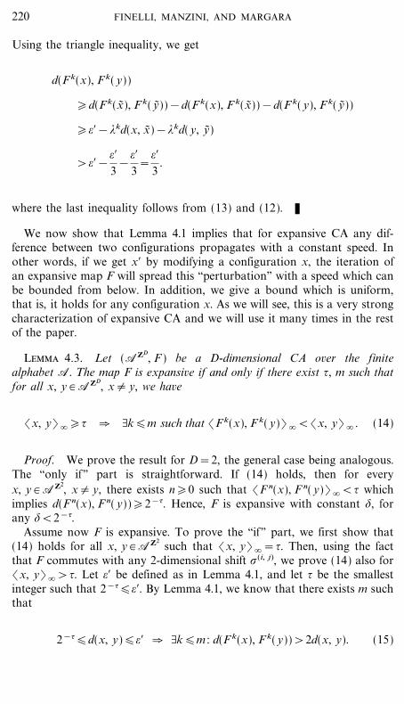
which implies (F k(x), F k( y)) �<{ as claimed.Consider now any t>{ and let (x, y) �=t. One can see that there

exists u� # Z2 such that &u� &�=t&{ and (_u� (x), _u� ( y)) �={ (see Fig. 1).Since (_u� (x), _u� ( y)) �={, we know that there exists k�m such that

[F k(_u� (x))](v� ){[F k(_u� ( y))](v� )

for some v� # Z2 with &v� &�<{. Since F k and _u� commutes, we get

[_u� (F k(x))](v� ){[_u� (F k(x))](u� ),

which implies

[F k(x)](v� +u� ){[F k( y)](v� +u� ).

This yields

(F k(x), F k( y)) ��&v� +u� &��&v� &�+&u� &�<{+(t&{)=t.

Hence, within m steps we have (F k(x), F k( y)) �<(x, y) � as claimed. K

FIG. 1. Each lattice represents a portion of Z2 centered at the origin (0, 0). Black circlesdenote the sites where configurations differ. We have (x, y) �={+2 (left), and (_(&2, &1)(x),_(&2, &1)( y)) �={ (right).



The characterization of Lemma 4.3 makes it possible to give an elemen-tary proof of the non-existence of D-dimensional CA for D�2. Our proofuses a pigeon-hole argument to show that, for D�2, differences amongconfigurations cannot propagate with a constant speed as required byLemma 4.3. We include this proof since it is considerably simpler than theproof given in [19].

Theorem 4.4. There are no expansive D-dimensional CA for D�2.

Proof. Let p=|A|. We prove the result for D=2, but the same reason-ing can be applied for all D�2. For any positive integer t, we define theset Qt /Z2 as

Qt=[v� # Z2 | &v� &��t].

Clearly, |Qt |=(2t+1)2. Assume F is expansive, and let {, m denote thevalues given by Lemma 4.3. Let z be any configuration in AZ2

. For r>{we define Bz, r as the set of configurations which coincide with z outside Qr .That is,

Bz, r=[x # AZ2| x(v� )=z(v� ) \v� � Qr].

Clearly, |Bz, r |= p |Qr|= p(2r+1)2. Consider now any pair x, y # Bz, r . We

have (x, y)��r, hence, by Lemma 4.3,

_k, 0�k�(r&{) m, such that (F k(x), F k( y)) ��{. (16)

In other words, for some k�m the two configurations F k(x) and F k( y)must differ inside Q{ . We prove that F cannot be expansive by showingthat this is not possible for all pairs x, y # Bz, r . For any configuration x, letx(Q{) denote the set of values assumed by x inside Q{ . For x # Bz, r , wedefine the orbit of x as the set

Ox= .(r&{) m

i=0

[F i (x)](Q{).

The orbit Ox represents the values assumed inside Q{ by the sequence x,F(x), F 2(x), ..., F (r&{) m(x). If F is expansive, all orbits Ox , for x # Bz, r ,must be distinct (otherwise (16) is violated). We prove that this isimpossible by showing that, for r sufficiently large, the number of possibleorbits is less than |Bz, r |. The number of distinct orbits is given by( p |Q{| )(r&{) m which asymptotically is rp4{2(r&{) m. Since m and { are con-stants, we have that for r large enough this is less than |Bz, r |= p(2r+1)2

. K



An immediate consequence of Lemma 4.3 is that for expansive CALemma 4.1 holds in a much stronger sense. More precisely, we can find alower bound to the number of iterations required to double the originaldistance which holds even for arbitrarily close points.

Corollary 4.5. Let (AZ, F ) be an expansive 1-dimensional CA. Then,there exist =>0 and an integer n such that

\x, y # X, 0{d(x, y)�= O _k�n : d(F k(x), F k( y))�2d(x, y). (17)

Note that Lemma 4.3 holds independently of the particular metric weuse. This is not true for Corollary 4.5. In fact, it takes little effort to provethat there exist metrics which induce the product topology for whichCorollary 4.5 does not hold (see for example the metric proposed in [11]).

5. EXPANSIVITY AND LYAPUNOV EXPONENTS INCELLULAR AUTOMATA

In the previous section we have shown that for any expansive CA thereis a lower bound to the speed at which ``perturbations'' propagate(Lemma 4.3 and Corollary 4.5). A remarkable consequence of this fact isthat expansive CA have positive Lyapunov exponents. In order to provethis result we need a preliminary lemma.

Lemma 5.1. Let (AZ, F ) be an expansive 1-dimensional CA. For everyx # AZ, let 4+

n (x), 4&n (x) be defined as in Section 3. Then, there exists a

constant c>0 such that

lim supn � �

1n

4+n (x)�c and lim sup

n � �

1n

4&n (x)�c.

Proof. Since F is expansive, by Lemma 4.3 we can find {, m such that

\y, z # AZ ( y, z)��{ O _k�m: (F k( y), F k(z))�<( y, z)� . (18)

We prove the lemma by showing that there exists an infinite set of integers[nj] j>0 such that

1nj

4&nj

(x)�1m

(the proof for 4+n (x) is similar).



Let x~ be a configuration such that x~ (0){x(0) and x~ (i)=x(i) for i{0.For any integer j>0, let yj=_ j+{(x) and y~ j=_ j+{(x~ ). By construction, wehave

( yj , y~ j) �= j+{. (19)

By applying (18) j times we get that there exists nj� jm such that

(F nj ( yj), F nj ( y~ j)) ��{. (20)

This means that while yj=_ j+s(x) and y~ j=_ j+s(x~ ) differ only at positionj+{, F nj ( yj) and F nj ( y~ j) must be differ at positions �{. Since 4&

nj(x)

measures how far a perturbation can move left in nj steps, we have

1nj

4&nj

(x)�j

nj�

1m

as claimed. To complete the proof we must show that the set [nj]j>0

contains an infinite number of elements. To see this note that, by (19) and(20), we have

d( yj , y~ j)=2& j&{ and d(F nj ( yj), F nj ( y~ j))�2&{,

which yields

d(F nj ( yj), F nj ( y~ j))�2 jd( y j , y~ j).

Since F is a Lipschitz function, we must have nj> j�log2 * which proves ourclaim. K

We are now ready to prove the main result concerning Lyapunovexponents.

Theorem 5.2. let (AZ, F ) be an expansive 1-dimensional CA, and let Ydenote the subset of AZ for which the right and left Lyapunov exponents(*+ and *&) exist. Then, there exists a constant c>0 such that for all x # Y,

*+(x)�c and *&(x)�c.

Moreover, for any _ invariant and F-invariant measure + there exists a+-measurable set Z+ such that Z+ �Y and +(Z+)=1.



Proof. Since *+(x) and *&(x) are defined as

*+(x)= limn � �

1n

4+n (x), *&(x)= lim

n � �

1n

4&n (x)

if the limits exist they cannot be smaller than the constant c given byLemma 5.1. The second part of the theorem follow directly by Theorem 3.1. K

Note that, if F is expansive it is also surjective (see for example [9]). Bya result in [6] we know that the Haar measure is F-invariant and_-invariant and therefore satisfies the hypothesis of Theorem 5.2.

6. EXPANSIVITY OVER INVARIANT SUBSPACES

In this section we prove that there exist non-expansive D-dimensionalCA which are expansive on a subset Y of the whole phase space. Moreover,the subset Y can be chosen to be a dense subset of the whole space. ForD�2 this result is particularly significant since it shows that expansivitycan be achieved if we restrict our attention to suitable subset of theconfiguration space AZD

.A similar analysis, applied to different dynamical properties (topological

transitivity and sensitivity to initial conditions), has been carried out byKnudsen [14] in the general framework of continuous transformations ofbounded metric spaces. He proved the following result.

Theorem 6.1 [14]. Let F : X � X, be a continuous transformation of abounded metric space (X, d ). Let Y be a dense subset of X such thatF(Y )�Y. Then F is topologically transitive [resp. sensitive to initialconditions] over Y iff it is topologically transitive [resp. sensitive to initialconditions] over X.

Given a CA (AZD, F ) we say that X�AZD

is an invariant subspace iffF(X )�X. If X is invariant, we say that (X, F ) is a subsystem of (AZD

, F ).If X is also a dense subset of AZD

we say that (X, F ) is a dense subsystemof (AZD

, F ). Note that X is a dense subset of AZDiff for every x # AZD

andk>0 there exists x$ # X such that (x, x$) �>k.

Theorem 6.1 guarantees that if a map F is transitive [sensitive] over aparticular dense invariant subset of the phase space, then F is transitive[sensitive] over any other dense invariant subset and on the whole space.The results of this section show that expansive maps have a differentbehavior.



Theorem 6.2. There exists a CA ([0, 1]Z, F ) which is not expansive butit has an expansive dense subsystem (X, F ).

Proof. Let F : [0, 1]Z � [0, 1]Z be defined by

[F(x)](i)=(x(i)+x(i+1)) mod 2 x # [0, 1]Z, i # Z. (21)

F is a linear map and it is not expansive by Theorem 7 in [16]. Let

X=[x # [0, 1]Z : _k(x)=x for some k>0]

denote the set of spatially periodic configurations. One can easily verifythat (X, F ) is a dense subsystem of ([0, 1]Z, F ). We prove the theorem byshowing that F is expansive over X.

Given any pair of distinct configurations x, y # X, let k, h>0 be suchthat x=_k(x) and y=_h( y). Then, for every m # Z,

x(i){ y(i) O x(i+mkh){ y(i+mkh). (22)

For x, y # X, define

(x, y) +�=min[i�0: x(i){ y(i)], (x, y) &

�=max[i<0: x(i){ y(i)].

The symbol (x, y) +� [(x, y) &

�] denotes the smallest non-negative [thelargest negative] position in which x and y differ. Both (x, y) +

� and(x, y) &

� are well defined in view of (22). By (21) we have

(x, y) &�<(x, y) +

�&1 O {(F(x), F( y)) &��(x, y) &

�

(F(x), F( y)) +�=(x, y) +

�&1(23)

We prove that F is expansive over X with parameter $=1�2. Let x, y # Xbe such that d(x, y)�1�8; by (2) we have

(x, y) &��&3 and (x, y) +

��3.

By (23) we get that after k=(x, y) +�&1 iterations (F k(x), F k( y)) +

�=1,which implies d(F k(x), F k( y))>1�2.

This completes the proof. K

Note that a result similar to Corollary 4.5 cannot hold if a map Fis expansive only over a dense subspace X/AZ. That is, the number ofiterations required to double the distance between two configurationscannot be uniformly bounded. Analogously, a result similar to Lemma 4.3



does not hold for expansive subsystems. For example, for the subsystemgiven in Theorem 6.2 it easy to see that for every t�1 and n>0 thereexist xn , yn # X such that (xn , yn) �=t and (F i (xn), F i ( yn)) ��t fori=1, ..., n.

We now show that also in the 2-dimensional case there exist (non-expan-sive) CA which are expansive over a dense subset of the whole space. Notethat the construction given below can be easily generalized to show thatthe same result holds true also for D>2.

Theorem 6.3. There exists a 2-dimensional CA ([0, 1]Z2, F ) which has

an expansive dense subsystem (Y, F ).

Proof. Let F#_(&1, &1). The map F is simply a one-step shift in thedirection of the main diagonal of the lattice. The construction of the subsetY over which F is expansive is quite complex. The basic idea is to force anypair of configurations x, y # Y to differ on infinitely many positions situatedalong the main diagonal of the lattice. The iteration of the map F will moveone of these differences to position (0, 0) so that, by (2), for some k>0 wehave d(F k(x), F k( y))=1.

Let X denote the set of configurations x # [0, 1]Z2such that: (a) there

exists only a finite number of pairs (i, j) such that i{ j and x(i, j){0, and(b) there exists k # Z such that for every i>k we have x(i, i)=0. We splitany configuration x # X into two parts: the body and the tail. The body Bx

of x is the smallest square region of the lattice which satisfies the followingproperties:

1. the cells on the diagonal of Bx have coordinates (i, i), i.e., thediagonal of Bx lies on the main diagonal of the lattice;

2. each cell not in Bx which contains 1 lies on the main diagonal ofthe lattice, that is, Bx contains all off-diagonal 1's;

3. let (u, u) denote the coordinates of the upper right corner of Bx ;for every i>u we have x(i, i)=0.

Let (l, l ) denote the coordinates of the lower left corner of Bx . The tailTx of x is defined by

Tx=[x(l&1, l&1), x(l&2, l&2), x(l&3, l&3), ...].

Note that, by construction, all nonzero cells of x belongs to Bx _ Tx . LetC be the map which associates to each body Bx the binary sequenceobtained by reading the entries of Bx row by row, left to right, from topto bottom. Let E : [0, 1]* � N be any injective map, where [0, 1]* denotes


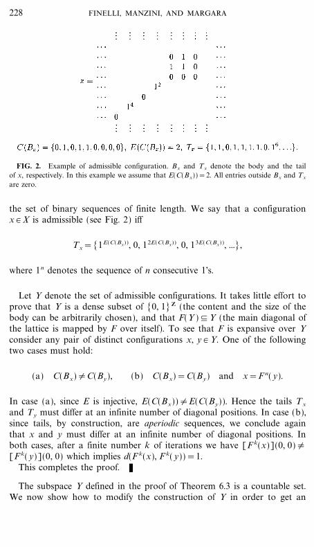
FIG. 2. Example of admissible configuration. Bx and Tx denote the body and the tailof x, respectively. In this example we assume that E(C(Bx))=2. All entries outside Bx and Tx

are zero.

the set of binary sequences of finite length. We say that a configurationx # X is admissible (see Fig. 2) iff

Tx=[1E(C(Bx)), 0, 12E(C(Bx)), 0, 13E(C(Bx)), ...],

where 1n denotes the sequence of n consecutive 1's.

Let Y denote the set of admissible configurations. It takes little effort toprove that Y is a dense subset of [0, 1]Z (the content and the size of thebody can be arbitrarily chosen), and that F(Y )�Y (the main diagonal ofthe lattice is mapped by F over itself). To see that F is expansive over Yconsider any pair of distinct configurations x, y # Y. One of the followingtwo cases must hold:

(a) C(Bx){C(By), (b) C(Bx)=C(By) and x=F n( y).

In case (a), since E is injective, E(C(Bx)){E(C(By)). Hence the tails Tx

and Ty must differ at an infinite number of diagonal positions. In case (b),since tails, by construction, are aperiodic sequences, we conclude againthat x and y must differ at an infinite number of diagonal positions. Inboth cases, after a finite number k of iterations we have [F k(x)](0, 0){[F k( y)](0, 0) which implies d(F k(x), F k( y))=1.

This completes the proof. K

The subspace Y defined in the proof of Theorem 6.3 is a countable set.We now show how to modify the construction of Y in order to get an



uncountable subspace Y$ such that (Y$, F ) is still an expansive dense sub-system.

We use the notation introduced in the proof of Theorem 6.3. Let x # Xand n=E(C(Bx)). Now we say that x is an admissible configuration if

Tx=[1n, 0, a1 , 0, 12n, 0, a2 , 0, 13n, ..., 1 in, 0, ai , 0, 1(i+1) n, ...],

where the binary sequence [aj] j # N is any sequence which satisfies thefollowing conditions:

1. aq=0, if q is not a prime power;

2. apn=apm , for every prime p and every pair of positive integers n, m.

Let Y$ denote the new set of admissible configurations. Note that, sincethere are infinitely many primes, there are uncountable many sequences[aj] j # N which can appear in the tail of admissible configurations. Hence,the set Y$ is uncountable. With some additional work with respect to theproof of Theorem 6.3 it is possible to prove that any pair of distinctconfigurations x, y # Y$ must differ on infinitely many diagonal positions.This implies that (Y$, F ) is expansive subsystem as claimed.

7. EXPANSIVITY VERSUS SENSITIVITY INCELLULAR AUTOMATA

In this section we consider sensitive Lipschitz functions over compactmetric spaces. Since the definitions of sensitivity and expansivity aresimilar, it is natural to ask whether results analogous to Lemma 4.1 andCorollary 4.5 hold true also for sensitive CA. As we will see, this is not thecase since sensitive and expansive maps turn out to have a quite differentbehavior.

The following example shows a sensitive 1-dimensional Ca (AZ, F ) suchthat

\n _=n , xn : d(xn , y)�=n

O d(F k(xn), F k( y))�2d(xn , y) for 0�k�n. (24)

In other words, there is no upper bound to the number of iterationsrequired to double the distance between two arbitrarily close configura-tions or, equivalently, there is no upper bound to the number of iterationsrequired to move a perturbation front of at least one position.


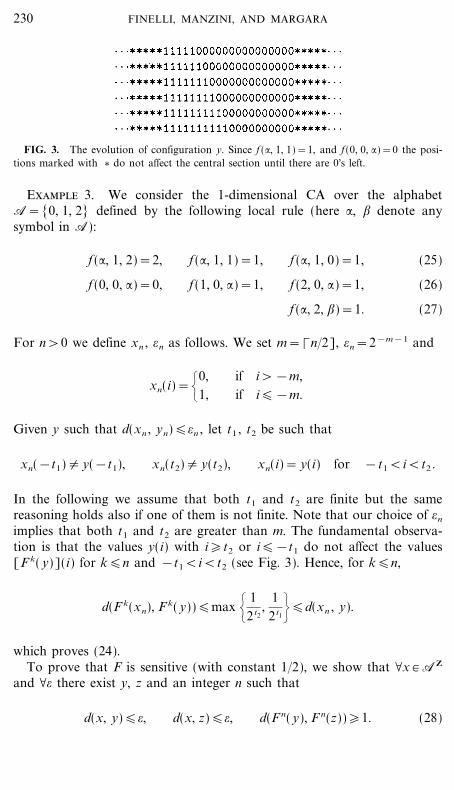
FIG. 3. The evolution of configuration y. Since f (:, 1, 1)=1, and f(0, 0, :)=0 the posi-tions marked with V do not affect the central section until there are 0's left.

Example 3. We consider the 1-dimensional CA over the alphabetA=[0, 1, 2] defined by the following local rule (here :, ; denote anysymbol in A):

f (:, 1, 2)=2, f (:, 1, 1)=1, f (:, 1, 0)=1, (25)

f (0, 0, :)=0, f (1, 0, :)=1, f (2, 0, :)=1, (26)

f (:, 2, ;)=1. (27)

For n>0 we define xn , =n as follows. We set m= Wn�2], =n=2&m&1 and

xn(i)={0, if i>&m,1, if i�&m.

Given y such that d(xn , yn)�=n , let t1 , t2 be such that

xn(&t1){ y(&t1), xn(t2){ y(t2), xn(i)= y(i) for &t1<i<t2 .

In the following we assume that both t1 and t2 are finite but the samereasoning holds also if one of them is not finite. Note that our choice of =n

implies that both t1 and t2 are greater than m. The fundamental observa-tion is that the values y(i) with i�t2 or i�&t1 do not affect the values[F k( y)](i) for k�n and &t1<i<t2 (see Fig. 3). Hence, for k�n,

d(F k(xn), F k( y))�max { 12t2

,1

2t1=�d(xn , y).

which proves (24).To prove that F is sensitive (with constant 1�2), we show that \x # AZ

and \= there exist y, z and an integer n such that

d(x, y)�=, d(x, z)�=, d(F n( y), F n(z))�1. (28)


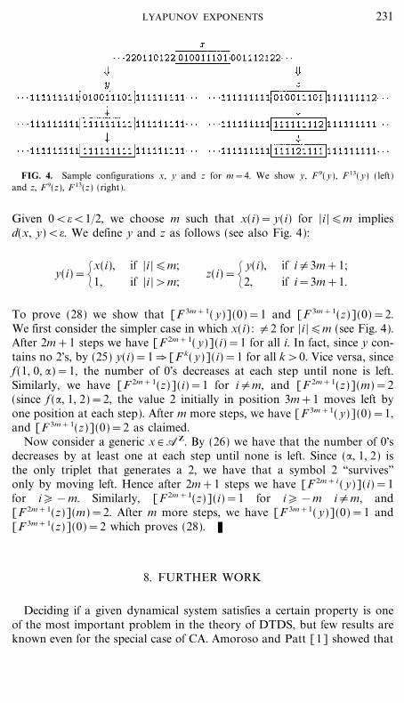
FIG. 4. Sample configurations x, y and z for m=4. We show y, F 9( y), F 13( y) (left)and z, F 9(z), F 13(z) (right).

Given 0<=<1�2, we choose m such that x(i)= y(i) for |i |�m impliesd(x, y)<=. We define y and z as follows (see also Fig. 4):

y(i)={x(i),1,

if |i |�m;if |i |>m;

z(i)={ y(i),2,

if i{3m+1;if i=3m+1.

To prove (28) we show that [F 3m+1( y)](0)=1 and [F 3m+1(z)](0)=2.We first consider the simpler case in which x(i) : {2 for |i |�m (see Fig. 4).After 2m+1 steps we have [F 2m+1( y)](i)=1 for all i. In fact, since y con-tains no 2's, by (25) y(i)=1 O [F k( y)](i)=1 for all k>0. Vice versa, sincef (1, 0, :)=1, the number of 0's decreases at each step until none is left.Similarly, we have [F 2m+1(z)](i)=1 for i{m, and [F 2m+1(z)](m)=2(since f (:, 1, 2)=2, the value 2 initially in position 3m+1 moves left byone position at each step). After m more steps, we have [F 3m+1( y)](0)=1,and [F 3m+1(z)](0)=2 as claimed.

Now consider a generic x # AZ. By (26) we have that the number of 0'sdecreases by at least one at each step until none is left. Since (:, 1, 2) isthe only triplet that generates a 2, we have that a symbol 2 ``survives''only by moving left. Hence after 2m+1 steps we have [F 2m+i ( y)](i)=1for i�&m. Similarly, [F 2m+1(z)](i)=1 for i�&m i{m, and[F 2m+1(z)](m)=2. After m more steps, we have [F 3m+1( y)](0)=1 and[F 3m+1(z)](0)=2 which proves (28). K

8. FURTHER WORK

Deciding if a given dynamical system satisfies a certain property is oneof the most important problem in the theory of DTDS, but few results areknown even for the special case of CA. Amoroso and Patt [1] showed that



surjectivity and injectivity of 1-dimensional CA are decidable properties,while Kari [12] proved that the same properties are undecidable in anydimension greater than 1. The decidability of expansivity and other topo-logical properties (such as sensitivity, transitivity, denseness of periodicorbits, etc.) are challenging open problems.

Our results suggest that expansivity of CA could be a decidable property.The crucial observation is that Lemma 4.3 guarantees that an expansivebehavior must become apparent, i.e., algorithmically detectable, aftera bounded number of iterations. Indeed, using Lemma 4.3 and working outsome hairy details, it is possible to prove that expansivity is at least semi-decidable, i.e., there exists an algorithm which, in finite time, answersyes if it receives as input an expansive CA. We are currently investigatingalgorithms for testing non-expansivity.

ACKNOWLEDGMENT

We thank A. Maass for the many valuable comments on an early version of the manuscript.

REFERENCES

1. Amoroso, S., and Patt, Y. (1972), Decision procedures for surjectivity and injectivity ofparallel maps for tessellation structures, J. Comput. System Sci. 6, 448�464.

2. Assaf, D., IV, and Coppel, W. A. (1992), Definition of chaos, Amer. Math. Monthly 99,865.

3. Banks, J., Brooks, J., Cairns, G., Davis, G., and Stacey, P., (1992), On the Devaney'sdefinition of chaos, Amer. Math. Monthly 99, 332�334.

4. Blanchard, F., Kurka, P., and Maass, A. (1997), Topological and measure-theoreticproperties of one-dimensional cellular automata, Physica D 103, 86�99.

5. Cattaneo, G., Formenti, G., Margara, L., and Mazoyer, J. (1997), A shift-invariant metricon SZ inducing a non-trivial topology, in ``22nd International Symposium on Mathemati-cal Foundations of Computer Science (MFCS'97),'' Springer-Verlag, Berlin�New York.

6. Coven, E., and Paul, M. (1974), Endomorphisms of irreducible subshifts of finite type,Math. Systems Theory 8, 167�175.

7. Denker, M., Grillenberger, C., and Sigmund, K. (1976), `Èrgodic Theory on CompactSpaces,'' Lecture Notes in Mathematics, Vol. 127, Springer-Verlag, Berlin�New York.

8. Devaney, R. L. (1989), `Àn Introduction to Chaotic Dynamical Systems,'' Addison�Wesley, Reading, MA.

9. Fagnani, F., and Margara, L. Expansivity, permutivity, and chaos for cellular automata,Theory Comput. Systems, to appear.

10. Garzon, M. (1995), ``Models of Massive Parallelism,'' EATCS Texts in Theoretical Com-puter Science, Springer-Verlag, Berlin�New York.

11. Hedlund, G. A. (1969), Endomorphism and automorphism of the shift dynamical system,Math. Systems Theory 3, 320�375.



12. Kari, J. (1994), Reversibility and surjectivity problems of cellular automata, J. Comput.System Sci. 48, 149�182.

13. Knudsen, C. (1994), `Àspects on Noninvertible Dynamics and Chaos,'' Ph.D. thesisPhysics Department, Technical University of Denmark.

14. Knudsen, C. (1994), Chaos without nonperiodicity, Amer. Math. Monthly 101, 563�565.

15. Kurka, P. (1997), Equicontinuity and attractors in cellular automata, Ergodic TheoryDynam. Systems 17, 417�433.

16. Manzini, G., and Margara, L. (1997), A complete and efficiently computable topologicalclassification of D-dimensional linear cellular automata over Zm, in ``24th InternationalColloquium on Automata Languages and Programming (ICALP'97),'' Springer-Verlag,Berlin�New York.

17. Martelli, M. (1994), ``Discrete Dynamical Systems and Chaos,'' Pitman Monographs andSurveys in Pure and Applied Science, Vol. 62, Longman, Harlow�New York.

18. Shereshevsky, M. A. (1992), Lyapunov exponents for one-dimensional cellular automata,J. Nonlinear Sci. 2, 1�8.

19. Shereshevsky, M. A. (1993), Expansiveness, entropy and polynomial growth for groupsacting on subshifts by automorphisms, Indag. Math. (N.S) 4, 203�210.

20. Vellekoop, M., and Berglund, R. (1994), On intervals, transitivity=chaos, Amer. Math.Monthly 101, 353�355.

� � � � � � � � � �


Lyapunov Exponents versus Expansivity and Sensitivity in Cellular Automata

Documents