Lyapunov-Based Economic Model Predictive Control for ...

Lyapunov-Based Economic ModelPredictive Control for Detecting andHandling Actuator and SimultaneousSensor/Actuator Cyberattacks onProcess Control SystemsHenrique Oyama, Dominic Messina, Keshav Kasturi Rangan and Helen Durand*

Department of Chemical Engineering and Materials Science, Wayne State University, Detroit, MI, United States

The controllers for a cyber-physical system may be impacted by sensor measurementcyberattacks, actuator signal cyberattacks, or both types of attacks. Prior work in ourgroup has developed a theory for handling cyberattacks on process sensors. However,sensor and actuator cyberattacks have a different character from one another. Specifically,sensor measurement attacks prevent proper inputs from being applied to the process bymanipulating the measurements that the controller receives, so that the control law plays arole in the impact of a given sensor measurement cyberattack on a process. In contrast,actuator signal attacks prevent proper inputs from being applied to a process bybypassing the control law to cause the actuators to apply undesirable control actions.Despite these differences, this manuscript shows that we can extend and combinestrategies for handling sensor cyberattacks from our prior work to handle attacks onactuators and to handle cases where sensor and actuator attacks occur at the same time.These strategies for cyberattack-handling and detection are based on the Lyapunov-based economic model predictive control (LEMPC) and nonlinear systems theory. We firstreview our prior work on sensor measurement cyberattacks, providing several newinsights regarding the methods. We then discuss how those methods can beextended to handle attacks on actuator signals and then how the strategies forhandling sensor and actuator attacks individually can be combined to produce astrategy that is able to guarantee safety when attacks are not detected, even if bothtypes of attacks are occurring at once.We also demonstrate that the other combinations ofthe sensor and actuator attack-handling strategies cannot achieve this same effect.Subsequently, we provide a mathematical characterization of the “discoverability” ofcyberattacks that enables us to consider the various strategies for cyberattackdetection presented in a more general context. We conclude by presenting a reactorexample that showcases the aspects of designing LEMPC.

Keywords: cyber-physical system, economic model predictive control, nonlinear systems, cyberattack detection,sensor attack, actuator attack

Edited by:Gianvito Vilé,

Politecnico di Milano, Italy

Reviewed by:Jinfeng Liu,

University of Alberta, CanadaAlexander William Dowling,University of Notre Dame,

United States

*Correspondence:Helen Durand

[email protected]

Specialty section:This article was submitted to

Computational Methods in ChemicalEngineering,

a section of the journalFrontiers in Chemical Engineering

Received: 06 November 2021Accepted: 24 January 2022

Published: 01 April 2022

Citation:Oyama H, Messina D, Rangan KK and

Durand H (2022) Lyapunov-BasedEconomic Model Predictive Control forDetecting and Handling Actuator and

Simultaneous Sensor/ActuatorCyberattacks on Process

Control Systems.Front. Chem. Eng. 4:810129.

doi: 10.3389/fceng.2022.810129

Frontiers in Chemical Engineering | www.frontiersin.org April 2022 | Volume 4 | Article 8101291

ORIGINAL RESEARCHpublished: 01 April 2022

doi: 10.3389/fceng.2022.810129

http://crossmark.crossref.org/dialog/?doi=10.3389/fceng.2022.810129&domain=pdf&date_stamp=2022-04-01

https://www.frontiersin.org/articles/10.3389/fceng.2022.810129/full





http://creativecommons.org/licenses/by/4.0/

mailto:[email protected]

https://doi.org/10.3389/fceng.2022.810129

https://www.frontiersin.org/journals/chemical-engineering

www.frontiersin.org

https://www.frontiersin.org/journals/chemical-engineering#articles


https://www.frontiersin.org/journals/chemical-engineering#editorial-board

https://doi.org/10.3389/fceng.2022.810129

1 INTRODUCTION

Cyber-physical systems (CPSs) integrate various physicalprocesses with computer and communication infrastructures,which allows enhanced process monitoring and control.Although CPSs open new avenues for advanced manufacturing(Davis et al., 2015) in terms of increased production efficiency,the quality of the production, and cost reduction, this integrationalso opens these systems to malicious cyberattacks that canexploit vulnerable communication channels between thedifferent layers of the system. In addition to process andnetwork cybersecurity concerns, data collection devices such assensors and final control elements such as actuators (and signalsto or from them) are also potential candidates that can be subjectto cyberattacks (Tuptuk and Hailes, 2018). Sophisticated andmalicious cyberattacks may affect industrial profits and even posea threat to the safety of individuals working on site, whichmotivates attack-handling strategies that are geared towardproviding safety assurances for autonomous systems.

There exist multiple points of susceptibility in a CPSframework ranging from communication networks andprotocols to sensor measurement and control signaltransmission, requiring the development of appropriate controland detection techniques to tackle such cybersecurity challenges(Pasqualetti et al., 2013). To better understand these concerns,vulnerability identification (Ani et al., 2017) has been studied bycombining people, process, and technology perspectives. Aprocess engineering-oriented overview of different attackevents has been discussed in Setola et al. (2019) to illustratethe impacts on industrial control system platforms. In order toaddress concerns related to control components, resilient controldesigns based on state estimates have been proposed for detectingand preventing attacks in works such as Ding et al. (2020) andCárdenas et al. (2011), wherein the latter cyberattack-resilientcontrol frameworks compare state estimates based on models ofthe physical process and state measurements to detectcyberattacks. Ye and Luo (2019) address a scenario whereactuator faults and cyberattacks on sensors or actuators occursimultaneously by using a control policy based on the Lyapunovtheory and adaptation and Nussbaum-type functions.

Cybersecurity-related studies have also been carried out in thecontext of model-predictive control (MPC; Qin and Badgwell,2003), an optimization-based control methodology thatcomputes optimal control actions to a process. Specifically, fornonlinear systems, Durand (2018) investigated various MPCtechniques with economics-based objective functions [knownas economic model predictive controllers (EMPCs) (Ellis et al.,2014a; Rawlings et al., 2012)] when only false sensormeasurements are considered. Chen et al. (2020) integrated aneural network-based attack detection approach initiallyproposed in Wu et al. (2018) with a two-fold controlstructure, in which the upper layer is a Lyapunov-based MPCdesigned to ensure closed-loop stability after attacks are flagged.A methodology that may be incorporated as a criterion for EMPCdesign has been proposed in Narasimhan et al. (2021), in which acontrol parameter screening based on a residual-based attackdetection scheme classifies multiplicative sensor-controller

attacks on a process as “detectable,” “undetectable,” and“potentially detectable” under certain conditions. In addition, ageneral description of “cyberattack discoverability” (i.e., a certainsystem’s capability to detect attacks) without a rigorousmathematical formalism has been addressed in Oyama et al.(2021).

Prior work in our group has explored the interaction betweencyberattack detection strategies, MPC/EMPC design, and stabilityguarantees. In particular, our prior works have primarily focusedon studying and developing control/detection mechanisms forscenarios in which either actuators or sensors are attacked(Oyama and Durand, 2020; Rangan et al., 2021; Oyama et al.,2021; Durand and Wegener, 2020). For example, Oyama andDurand (2020) proposed three cyberattack detection conceptsthat are integrated with the control framework Lyapunov-basedEMPC (Heidarinejad et al., 2012a). Advancing this work, Ranganet al. (2021) and Oyama et al. (2021) proposed ways to considercyberattack detection strategies and the challenges in cyberattack-handling for nonlinear processes whose dynamics change withtime. In the present manuscript, we extend our prior work (whichcovered sensor measurement cyberattack-handling with control-theoretic guarantees and actuator cyberattack-handling withoutguarantees) to develop strategies for maintaining safety whenactuator attacks are not detected (assuming that no attack occurson the sensors). These strategies are inspired by the first detectionconcept in Oyama and Durand (2020) but with a modifiedimplementation strategy to guarantee that even when anundetected actuator attack occurs, the state measurement andactual closed-loop state are maintained inside a safe region ofoperation throughout the next sampling period.

The primary challenge addressed by this work is the questionof how to develop an LEMPC-based strategy for handling sensorand actuator cyberattacks occurring at once. The reason that thisis a challenge is that some of the concepts discussed for handlingsensor and actuator cyberattacks only work if the other (sensorsor actuators) is not under an attack. A major contribution of thepresent manuscript, therefore, is elucidating which sensor andactuator attack-handling methods can be combined to providesafety in the presence of undetected attacks, even if bothundetected sensor and actuator attacks are occurring at thesame time. To cast this discussion in a broader framework, wealso present a nonlinear systems definition of cyberattack“discoverability,” which provides fundamental insights intohow attacks can fly under the radar of detection policies.Finally, we elucidate the properties of cyberattack-handlingusing LEMPC through simulation studies.

The manuscript is organized as follows: following somepreliminaries that clarify the class of systems underconsideration and the control design (LEMPC) from whichthe cyberattack detection and handling concepts presented inthis work are derived, we review the sensor measurementcyberattack detection and handling policies from Oyama andDurand (2020), which form the basis for the development of theactuator signal cyberattack-handling and combined sensor/actuator cyberattack-handling policies subsequently developed.Subsequently, we propose strategies for detecting and handlingcyberattacks on process actuators when the sensor measurements


Oyama et al. LEMPC for Simultaneous Sensor and Actuator Cyberattacks


www.frontiersin.org


remain intact that are able to maintain safety even when actuatorcyberattacks are undetected. We then utilize the insights anddevelopments of the prior sections to clarify which sensor andactuator attack-handling policies can be combined to achievesafety in the presence of combined sensor and actuatorcyberattacks. We demonstrate that there are combinations ofmethods that can guarantee safety in the presence of undetectedattacks, even if these attacks occur on both sensors and actuatorsat the same time (though the other combinations of the discussedmethods cannot achieve this). Further insights on the interactionsbetween the detection strategies and control policies for nonlinearsystems are presented via a fundamental nonlinear systemsdefinition of discoverability. The work is concluded with areactor study that probes the question of the practicality of thedesign of control systems that meet the theoretical guarantees forachieving cyberattack-resilience.

2 PRELIMINARIES

2.1 NotationThe Euclidean norm of a vector is indicated by |·|, and thetranspose of a vector x is denoted by xT. A continuousfunction α: [0, a) → [0, ∞) is said to be of class K if it isstrictly increasing and α(0) = 0. Set subtraction is designated byx ∈ A/B ≔ {x ∈ Rn : x ∈ A, x∉B}. Finally, a level set of a positivedefinite function V is denoted by Ωρ ≔ {x ∈ Rn : V(x) ≤ ρ}.

2.2 Class of SystemsThis work considers the following class of nonlinear systems:

_x t( ) � f x t( ), u t( ), w t( )( ) (1)where x ∈ X ⊂ Rn and w ∈W ⊂ Rz (W≔{w ∈ Rz | |w| ≤ θw, θw > 0})are the state and disturbance vectors, respectively. The inputvector function u ∈ U ⊂ Rm, where U≔{u ∈ Rm| |u| ≤ umax}. f islocally Lipschitz on X × U × W, and we consider that the“nominal” system of Eq. 1 (w ≡ 0) is stabilizable such thatthere exist an asymptotically stabilizing feedback control lawh(x), a sufficiently smooth Lyapunov function V, and class Kfunctions αi(·), i = 1, 2, 3, 4, where

α1 |x|( )≤V x( )≤ α2 |x|( ) (2a)zV x( )zx

f x, h x( ), 0( )≤ − α3 |x|( ) (2b)zV x( )zx

∣∣∣∣∣∣∣∣∣∣∣∣∣∣≤ α4 |x|( ) (2c)

h x( ) ∈ U (2d)∀ x ∈D ⊂ Rn (D is an open neighborhood of the origin). We defineΩρ ⊂ D to be the stability region of the nominal closed-loopsystem under the controller h(x) and require that it be chosensuch that x ∈ X, ∀x ∈ Ωρ. Furthermore, we consider that h(x)satisfies the following equation:

|hi x( ) − hi x( )|≤ Lh|x − x| (3)for all x, x ∈ Ωρ, with Lh > 0, where hi is the i-th component of h.

Since f is locally Lipschitz and V(x) is a sufficiently smoothfunction, the following holds:

|f x1, u, w( ) − f x2, u, 0( )|≤ Lx|x1 − x2| + Lw|w| (4a)zV x1( )zx

f x1, u, w( ) − zV x2( )zx

f x2, u, 0( )∣∣∣∣∣∣∣

∣∣∣∣∣∣∣≤ Lx′ |x1 − x2|+ Lw′ |w| (4b)

|f x1, u1, w( ) − f x1, u2, w( )|≤ Lu|u1 − u2| (4c)|f x, u, w( )|≤Mf (5)

∀x1, x2 ∈ Ωρ, u, u1, u2 ∈ U and w ∈ W, where Lx, Lx′ , Lw, Lw′ , Lu,and Mf are positive constants.

We also assume that there are M sets of measurementsyi ∈ Rqi , i = 1, . . . , M, available at tk as follows:

yi t( ) � ki x t( )( ) + vi t( ) (6)where ki is a vector-valued function, and vi represents themeasurement noise associated with the measurements yi. Weassume that the measurement noise is bounded(i.e., vi ∈ Vi ≔ vi ∈ Rqi | |vi|≤ θv,i, θv,i > 0{ ) and thatmeasurements of each yi are continuously available. For eachof the M sets of measurements, we assume that there exists adeterministic observer [e.g., a high-gain observer Ahrens andKhalil (2009)] described by the following dynamic equation:

_zi � Fi ϵi, zi, yi( ) (7)where zi is the estimate of the process state from the i-th observer,i = 1, . . . , M, Fi is a vector-valued function, and ϵi > 0. When acontroller h(zi) with Eq. 7 is used to control the closed-loopsystem of Eq. 1, we consider that Assumption 1 and Assumption2 below hold.

Assumption 1. Ellis et al. (2014b), Lao et al. (2015) There existpositive constants θpw, θ

pv,i, such that for each pair {θw, θv,i} with

θw ≤ θpw, θv,i ≤ θpv,i, there exist 0 < ρ1,i < ρ, em0i > 0 and ϵpLi > 0,

ϵpUi > 0 such that if x(0) ∈ Ωρ1,i, |zi(0)−x(0)| ≤ em0i, andϵi ∈ (ϵpLi, ϵpUi), the trajectories of the closed-loop system arebounded in Ωρ, ∀ t ≥ 0.

Assumption 2. Ellis et al. (2014b), Lao et al. (2015) There existsepmi > 0 such that for each emi ≥ epmi, there exists tbi(ϵi) such that|zi(t) − x(t)|≤ emi, ∀ t≥ tbi(ϵi).

3 ECONOMIC MODEL PREDICTIVECONTROL

EMPC Ellis et al. (2014a) is an optimization-based control designfor which the control actions are computed via the followingoptimization problem:

minu t( )∈S Δ( )

∫tk+N

tk

Le ~x τ( ), u τ( )( ) dτ (8a)

s.t. _~x t( ) � f ~x t( ), u t( ), 0( ) (8b)~x tk( ) � x tk( ) (8c)




www.frontiersin.org


~x t( ) ∈ X, ∀ t ∈ tk, tk+N[ ) (8d)u t( ) ∈ U, ∀ t ∈ tk, tk+N[ ) (8e)

where N is called the prediction horizon, and u(t) is a piecewise-constant input trajectory with N pieces, where each piece is heldconstant for a sampling period with time length Δ. Theeconomics-based stage cost Le of Eq. 8a is evaluatedthroughout the prediction horizon using the future predictionsof the process state ~x from the model of Eq. 8b (the nominalmodel of Eq. 1) initialized from the state measurement at tk (Eq.8c). The process constraints of Eq. 8d, Eq. 8e are state and inputconstraints, respectively. A receding or moving horizonimplementation strategy is employed, i.e., the optimizationproblem is solved every Δ time units (at each sampling timetk) such that the first of the N pieces of the input vector trajectorythat is the optimal solution is applied to the process. The optimalsolution at tk is denoted by up(ti|tk), where i = k, . . . , k + N−1.

Additional constraints that can be added to the formulation inEq. 8 to produce a formulation of EMPC that takes advantage ofthe Lyapunov-based controller h(·), called Lyapunov-basedEMPC [LEMPC Heidarinejad et al. (2012a)], are as follows:

V ~x t( )( )≤ ρe′, ∀ t ∈ tk, tk+N[ ), if x tk( ) ∈ Ωρe′ (9a)zV ~x tk( )( )

zxf ~x tk( ), u tk( ), 0( )

≤zV ~x tk( )( )

zxf ~x tk( ), h ~x tk( )( ), 0( ), if ~x tk( ) ∈ Ωρ/Ωρe′

(9b)

where Ωρe′ ⊂ Ωρ is a subset of the stability region that makes Ωρ

forward invariant under the controller of Eqs 8–9.

4 CYBERATTACK DETECTION ANDCONTROL STRATEGIES USING LEMPCUNDER SINGLE ATTACK-TYPESCENARIOS: SENSOR ATTACKS

The major goal of this work is to extend the strategies for LEMPC-based sensor measurement cyberattack detection and handlingfrom Oyama and Durand (2020) to handle actuator attacks andsimultaneous sensor measurement and actuator attacks. For theclarity of this discussion, we first review the three cyberattackdetection mechanisms from Oyama and Durand (2020).

This section therefore considers a single attack-type scenario(i.e., only the sensor readings are impacted by attacks). The firstcontrol/detection strategy proposed in Oyama and Durand (2020)switches between a full-state feedback LEMPC and variations onthat control design that are randomly generated over time to probefor cyberattacks by evaluating state trajectories for which it istheoretically known that a Lyapunov function must decreasebetween subsequent sampling times. The second control/detection strategy also uses full-state feedback LEMPC, but thedetection is achieved by evaluating the state predictions based onthe current and prior state measurements to flag an attack whilemaintaining the closed-loop state within a predefined safe regionover one sampling period after an undetected attack is applied. The

third control/detection strategy was developed using outputfeedback LEMPC, and the detection is attained by checkingamong multiple redundant state estimates to flag that an attackis happening when the state estimates do not agree while stillensuring closed-loop stability under sufficient conditions (whichinclude the assumption that at least one of the estimators cannot beaffected by the attack). In addition to reviewing the key features ofthis design, this section will provide several clarifications that werenot provided in Oyama and Durand (2020) to enable us to buildupon these methods in future sections.

4.1 Control/Detection Strategy 1-S UsingLEMPC in the Presence of Sensor AttacksThe control/detection strategy 1-S, which corresponds to the firstdetection concept proposed in Oyama and Durand (2020), usesfull-state feedback LEMPC as the baseline controller and randomlydevelops other LEMPC formulations with Eq. 9b always activatedthat are used in place of the baseline controller for short periods oftime to potentially detect if an attack is occurring. We definespecific times at which the switching between the baseline 1-LEMPC and the j-th LEMPC, j > 1, happens. Particularly, ts,j isdefined as the switching time at which the j-LEMPC is used to drivethe closed-loop state to the randomly generated j-th steady-state,and te,j is the time at which the j-LEMPC switches back tooperation under the 1-LEMPC.

The baseline 1-LEMPC is formulated as follows, which is usedif te,j−1 ≤ t < ts,j, j = 2, . . . , where te,1 = 0:

minu1 t( )∈S Δ( )

∫tk+N

tk

Le ~x1 τ( ), u1 τ( )( ) dτ (10a)

s.t. _~x1 t( ) � f1 ~x1 t( ), u1 t( ), 0( ) (10b)~x1 tk( ) � x1 tk( ) (10c)

~x1 t( ) ∈ X1, ∀ t ∈ tk, tk+N[ ) (10d)u1 t( ) ∈ U1, ∀ t ∈ tk, tk+N[ ) (10e)

V1 ~x1 t( )( )≤ ρe,1′ , ∀ t ∈ tk, tk+N[ ), if ~x1 tk( ) ∈ Ωρe,1′ (10f )zV1 ~x1 tk( )( )

zxf1 ~x1 tk( ), u1 tk( ), 0( )

≤zV1 ~x1 tk( )( )

zxf1 ~x1 tk( ), h1 ~x1 tk( )( ), 0( ), if ~x1 tk( ) ∈ Ωρ1/Ωρe,1′

(10g)where x1(tk) is used, with a slight abuse of the notation, to reflectthe state measurement in a deviation variable form from theoperating steady state. In addition, in the remainder of this work,fi (i ≥ 1) represents the right-hand side of Eq. 1 when it is writtenin a deviation variable form from the i-th steady state. uirepresents the input vector in a deviation variable form fromthe steady-state input associated with the i-th steady state. Xi andUi correspond to the state and input constraint sets in a deviationvariable form from the i-th steady state. In addition, ρi and ρe,i′ areassociated with the i-th steady state. The addition of a subscript ito the functions in Eq. 2 (to form hi,Vi, and αj,i, j = 1, 2, 3, 4) orMf

also signifies association with the i-th steady state.The j-th LEMPC, j > 1, which is used for t ∈ [ts,j, te,j), is

formulated as follows:




www.frontiersin.org


minuj t( )∈S Δ( )

∫tk+N

tk

Le ~xj τ( ), uj τ( )( ) dτ (11a)

s.t. _~xj t( ) � fj ~xj t( ), uj t( ), 0( ) (11b)~xj tk( ) � xj tk( ) (11c)

~xj t( ) ∈ Xj, ∀ t ∈ tk, tk+N[ ) (11d)uj t( ) ∈ Uj, ∀ t ∈ tk, tk+N[ ) (11e)

zVj ~xj tk( )( )zx

fj ~xj tk( ), uj tk( ), 0( )≤zVj ~xj tk( )( )

zxfj ~xj tk( ), hj ~xj tk( )( ), 0( ) (11f )

where xj(tk) represents the state measurement in a deviationvariable form from the j-th steady state.

The implementation strategy for this detection method is asfollows (the stability region subsets are thoroughly detailed inOyama and Durand (2020) but reviewed in Remark 1):

1) At a sampling time tk, the baseline 1-LEMPC receives the statemeasurement ~x1(tk). Go to Step 2.

2) At tk, a random number ζ is generated. If this number fallswithin a range that has been selected to start probing forcyberattacks, randomly generate a j-th steady state, j > 1, witha stability region Ωρj ⊂ Ωρsamp2,1

that has a steady-state inputwithin the input bounds, contains the state measurement~xj(tk), and where ~xj(tk) ∈ Ωρh,j/Ωρs,j. Set ts,j = tk, choosete,j = tk+1, and go to Step 4. Otherwise, if ζ falls in a rangethat has not been chosen to start probing for cyberattacks orthe j-th steady state cannot be generated to meet theconditions above (which include the consideration of thedifferent levels of stability regions), go to Step 3.

3) If ~x1(tk) ∈ Ωρe,1′ , go to Step 3a. Else, go to Step 3b.a) Compute control signals for the subsequent sampling

period with Eq. 10f of the 1-LEMPC activated. Go toStep 6.

b) Compute control signals for the subsequent samplingperiod with Eq. 10g of the 1-LEMPC activated. Go toStep 6.

4) The j-LEMPC receives the state measurement ~xj(tk) andcontrols the process according to Eq. 11. Evaluate theLyapunov function profile throughout the sampling period.If Vj does not decrease by the end of the sampling periodfollowing ts,j, or if ~xj(t) ∉ Ωρ1 at any time for t ∈ [tk, tk+1),detect that the process is potentially under a cyberattack andmitigating actions may be applied. Otherwise, go to Step 5.

5) At te,j, switch back to operation under the baseline 1-LEMPC.Go to Step 6.

6) Go to Step 1 (k ← k + 1).

The first theorem presented in Oyama and Durand (2020) andreplicated below guarantees the closed-loop stability of theprocess of Eq. 1 under the LEMPCs of Eqs 10–11 under theimplementation strategy described above in the absence of sensorcyberattacks. To follow this and the other theorems that will bepresented in this work, the impacts of bounded measurementnoise and disturbances on the process state trajectory are

characterized in Proposition 1 below, and the bound on thevalue of the Lyapunov function at different points in the stabilityregion is defined in Proposition 2.

Proposition 1. Ellis et al. (2014b), Lao et al. (2015) Consider thesystems below:

_xi � fi xi t( ), ui t( ), w t( )( ) (12a)_~xi � fi ~xi t( ), ui t( ), 0( ) (12b)

where |xi(t0) − ~xi(t0)|≤ δ with t0 = 0. If xi(t), ~xi(t) ∈ Ωρi for t ∈[0, T], then there exists a function fW,i(·, ·) such that

|xi t( ) − ~xi t( )|≤fW,i δ, t − t0( ) (13)for all xi(t), ~xi(t) ∈ Ωρi, ui ∈ Ui, and w ∈ W, with

fW,i s, τ( ) ≔ s + Lw,iθwLx,i

( )eLx,iτ − Lw,iθwLx,i

(14)

Proposition 2. Ellis et al. (2014b) Let Vi(·) represent theLyapunov function of the nominal system of Eq. 1, in adeviation form from the i-th steady state, under the controllerhi(·) that satisfies Eqs 2, 3 for the system of Eq. 1 when it is in adeviation variable form from the i-th steady state. Then, thereexists a function fVi such that

Vi �x( )≤Vi �x′( ) + fVi |�x − �x′|( ) (15)∀�x, �x′ ∈ Ωρi where fVi(·) is given by

fVi s( ) ≔ α4,i α−11,i ρi( )( )s +MVis

2 (16)where MVi is a positive constant.

Theorem 1. Oyama and Durand (2020) Consider the closed-loopsystem of Eq. 1 under the implementation strategy described aboveand in the absence of a false sensor measurement cyberattackwhere each controller hj(·), j ≥ 1, used in each j-LEMPCmeets theinequalities in Eqs 2, 3 with respect to the j-th dynamic model.Let ϵWj > 0, Δ > 0, N≥ 1, Ωρj ⊂ Ωρsamp2,1 ⊂ Ωρ1 ⊂ X1 for j > 1,ρj > ρh,j > ρmin ,j > ρs,j > ρs,j′ > 0, where Ωρh,j is defined as thesmallest level set of Ωρj that guarantees that if Vj(~xj(tk))≤ ρh,j,Vj(xj(tk))≤ ρj, and ρ1 > ρsamp2,1 > ρsamp,1 > ρe,1′ > ρmin ,1 >ρs,1 > ρs,1′ > 0 (where Ωρsamp,1

is defined as a level set of Ωρ1 thatguarantees that if x1(tk) ∈ Ωρ1/Ωρsamp,1, then ~x1(tk) ∈ Ωρ1/Ωρe,1′ )satisfy

−α3,j α−12,j ρs,j′( )( ) + Lx,j′ Mf,jΔ≤ − ϵw,j/Δ, j � 1, 2, . . . (17)

ρe,1′ + fV,1 fW,1 δ,Δ( )( )≤ ρsamp2,1 (18)−α3,1 α−1

2,1 ρe,1′( )( ) + Lx,1′ Mf,1Δ + Lx,1′ δ + Lw,1′ θw ≤ − ϵw,1′ /Δ (19)−α3,j α−1

2,j ρs,j( )( ) + Lx,j′ Mf,jΔ + Lx,j′ δ + Lw,j′ θw ≤ − ϵw,j′ /Δ,j � 1, 2, 3, . . . (20)

ρmin ,j � max Vj xj t( )( ) : xj tk( ) ∈ Ωρs,j′ , t ∈ tk, tk+1[ ), uj ∈ Uj{ },j � 1, 2, . . . (21)




www.frontiersin.org


ρsamp2,1 ≥max V1 x1 t( )( ) : x1 tk( ) ∈ Ωρsamp,1/Ωρe,1′ ,{

t ∈ tk, tk+1[ ), u1 ∈ U1} (22)ρ1 ≥max V1 ~x1 tk( )( ): x1 tk( ) ∈ Ωρsamp2,1

{ } (23)ρj � max Vj xj tk( )( ): ~xj tk( ) ∈ Ωρh,j{ }, j � 2, 3, . . . (24)

ρs,j′ <min Vj xj tk( )( ): ~xj tk( ) ∈ Ωρj/Ωρs,j{ }, j � 1, 2, . . . (25)

If ~x1(t0) ∈ Ωρsamp2,1, x1(t0) ∈ Ωρsamp2,1

, and |~xj(tk) − xj(tk)|≤ δ, k= 0, 1, . . . , then the closed-loop state is maintained inΩρsamp2,1

andthe state measurement is inΩρ1 when the 1-LEMPC is activated att0 and for te,j−1 ≤ t< ts,j or when the j-LEMPC is activated forts,j ≤ t< te,j under the implementation strategy described above,and the closed-loop state and the state measurement aremaintained within Ωρ1 for t≥ 0. Furthermore, in the samplingperiod after ts,j, if ~xj(tk) ∈ Ωρj/Ωρs,j,Vj decreases and xj(t) ∈ Ωρjfor t ∈ [tk, tk+1).

An important clarification regarding the strategy describedabove that provides more detail compared to (Oyama andDurand, 2020) and aids in understanding the extensions ofthis method developed later in this work for handling actuatorattacks is that the decrease in Vj in Theorem 1 is a decrease in Vj

along the closed-loop state trajectory of the actual state (not themeasurement). Specifically, that statement in the theorem comesfrom the following equation in the proof of Theorem 1 inOyama and Durand (2020), which provides an upper boundon _Vj along the actual closed-loop state trajectory from tk totk+1 under an input computed by the j-LEMPC when followingthe implementation strategy described above (i.e., ~xj(tk) ∈ Ωρh,j/Ωρs,j)when Eq. 20 is satisfied:

zVj xj τ( )( )zx

fj xj τ( ), uj tk( ), w τ( )( )≤ − α3,j α−12,j ρs,j( )( )+ Lx,j′ Mf,jΔ + Lx,j′ δ + Lw,j′ θw ≤ − ϵw,j′ /Δ (26)

This expression indicates that Vj(xj(t))≤Vj(xj(t0))−ϵw,j′ (t−t0)

Δ , giving a minimum decrease in Vj of ϵw,j′ over thesampling period. If this decrease is enough to overcome anymeasurement noise, such as if

ϵw,j′ > max~xj tk( )∈Ωρh,j/Ωρs,j

min Vj ~xj tk( )( ): ~xj tk( ) ∈ Ωρh,j/Ωρs,j{ }∣∣∣∣∣∣∣∣

−max Vj ~xj tk+1( )( ): ~xj tk( ) ∈ Ωρh,j/Ωρs,j,{uj ∈ Uj, |xj tp( ) − ~xj tp( )|≤ θv,j, p � k, k + 1}| (27)

when the input is computed by the j-LEMPC (where θv,1represents the measurement noise when the full-state feedbackis available), then the state measurement must also be decreasedby the end of the sampling period. However, at any giventime instant, it is not guaranteed to be decreasing due to thenoise. An unusual amount of increase could help to flag theattack before a sampling period is over, although this would comefrom recognizing atypical behavior (essentially patternrecognition).

The reasoning behind the selection of the presented bound onϵw,j′ is as follows: the lack of a decrease in the Lyapunov functionvalue between tk and tk+1 is meant to flag an attack. However, withsensor noise, it is possible that Eq. 26 can hold (which reflects adecrease in the value of Vj evaluated along the trajectory of theactual closed-loop state) but that the decrease in Vj caused by Eq.26 is not enough to ensure that Vj evaluated at the measuredvalues of the closed-loop state (instead of the actual values)decreases between tk and tk+1. For example, consider the casein which the value of Vj barely decreases over a sampling period,so that Vj can be treated as approximately constant. If the noise inthe measurements is large, it may then be possible thatVj(~xj(tk))<Vj(~xj(tk+1)), even though Vj slightly decreasedalong the actual closed-loop state trajectory (if, for example,the noise originally takes Vj(~xj(tk)) to the minimum possiblevalue, it could be for a given Vj(xj(tk)), but then at the nextsampling time, the Lyapunov function evaluated at themeasurement is the maximum possible value that it couldtake). Equation 27 ensures that even if this occurs, thedecrease in Vj along the actual closed-loop state trajectory isenough to ensure that the maximum value of Vj(~xj(tk+1)) is lessthan the minimum value of Vj(~xj(tk)).

Remark 1. The following relation between the different stabilityregions has been characterized for Detection Strategy 1-S:ρ1 > ρsamp2,1 > ρsamp,1 > ρe,1′ > ρmin ,1 > ρs,1 > ρs,1′ > 0 (which musthold when the baseline 1-LEMPC is used) andρj > ρh,j > ρmin ,j > ρs,j > ρs,j′ > 0 for j > 1 (which must holdwhen the j-LEMPC is used). The regions Ωρsamp,1

, Ωρs,j, andΩρh,j are important to define due to the presence ofmeasurement noise (Oyama and Durand, 2020). Specifically,Ωρj, j = 1, 2, . . . has been defined as an invariant set in whichthe closed-loop state is maintained, andΩρe,1′ is a region utilized indistinguishing between whether Eq. 10f or Eq. 10g is activated inEq. 10. Ωρs,j′ , j = 1, 2, . . . , is defined as a region such that if theactual state is within Ωρs,j′ at a sampling time, the maximumdistance that the closed-loop state would be able to go within asampling period is into Ωρmin ,j

. Furthermore, we define the regionΩρs,j such that if the state measurement is within Ωρh,j/Ωρs,j at tk,the actual state is outside of Ωρs,j′ . Ωρsamp,1

is characterized as aregion where, if the actual state is inside this region at a samplingtime, the maximum distance that the closed-loop state would beable to travel within a sampling period is into Ωρsamp2,1

. Ωρsamp2,1is

then defined to be a subset of Ωρ1 so that the maximum distancethat the closed-loop state could go when the state measurement iswithin Ωρe,1′ but the actual state is outside of this region is stillinside Ωρ1. To ensure that the actual state at tk is inside Ωρj, wedefine the region Ωρh,j ⊂ Ωρj such that if the state measurement iswithin Ωρh,j at tk, the actual state is inside Ωρj.

4.2 Control/Detection Strategy 2-S UsingLEMPC in the Presence of Sensor AttacksThe control/detection strategy 2-S, which corresponds to thesecond detection concept in Oyama and Durand (2020), has beendeveloped using only the 1-LEMPC of Eq. 10, and it flags false




www.frontiersin.org


sensor measurements based on state predictions from the processmodel from the last state measurement. If the norm of thedifference between the state predictions and the currentmeasurements is above a threshold, the measurement isidentified as a potential sensor attack. Otherwise, if the normis below this threshold, even if the measurement was falsified, theclosed-loop state can be maintained inside Ωρ1, under sufficientconditions Oyama and Durand (2020), for a sampling periodafter the attack is applied for the process operated under anLEMPC that follows the implementation strategy below, where~x1(tk|tk−1) denotes the prediction of the state ~x1 at tk evaluated byintegrating the process model of Eq. 10b from a measurement attk−1 until tk:

1) At sampling time tk, if |~x1(tk|tk−1) − ~x1(tk|tk)|> ], flag that acyberattack is happening and go to Step 1a. Else, go to Step 1b.a) Mitigating actions may be applied (e.g., a backup policy

such as the use of redundant controller or an emergencyshut-down mode).

b) Operate the process under the 1-LEMPC of Eq. 10 whileimplementing an auxiliary detection mechanism toattempt to flag any undetected attack at tk. tk ← tk+1.Go to Step 1.

The second theorem presented in Oyama and Durand (2020),which is replicated below, guarantees the closed-loop stability ofthe process of Eq. 1 under the 1-LEMPC of Eq. 10 under theimplementation strategy described above before a sensor attackoccurs and for at least one sampling period after the attack.

Theorem 2. Oyama and Durand (2020) Consider the system ofEq. 1 in closed loop under the implementation strategy describedin Section 4.2 based on a controller h1(·) that satisfies theassumptions of Eqs 2, 3. Let the conditions of Theorem 1hold with ts,j � ∞, j = 2, 3, . . . , and δ ≥fW,1(θv,1,Δ) + ]. If~x1(t0) ∈ Ωρsamp2,1

⊂ Ωρ1 and x1(t0) ∈ Ωρsamp2,1, then x1(t) ∈ Ωρsamp2,1

and the state measurement at each sampling time is in Ωρ1 for alltimes before a sampling time tA that a cyberattack falsifies a statemeasurement, and x1(t) ∈ Ωρsamp2,1

for t ∈ [tA, tA + Δ), if theattack is not detected at tA.

In Theorem 2, δ represents the deviation between the statemeasurement and the actual state that can be tolerated with theprovided closed-loop stability guarantees. If there is no attack, δcorresponds to measurement noise. If there is an attack, then δreflects the largest possible deviation of the falsified statemeasurement from the actual state that can be tolerated whilethe guarantees in the theorem are obtained.

We now provide some additional insights into this strategycompared to Oyama and Durand (2020) in preparation for adiscussion about cyberattack “discoverability” later in this work.Specifically, the reason that closed-loop stability can only beguaranteed for a sampling period after an attack in Theorem 2is due to the use of a state prediction in detecting the attack.Specifically, Theorem 2 ensures that ~x1(t) ∈ Ωρ1 andx1(t) ∈ Ωρsamp2,1

for t < tA. According to Oyama and Durand(2020), to demonstrate that x1(t) ∈ Ωρsamp2,1

for t ∈ [tA, tA + Δ), weconsider the measurements ~x1(tk−1|tk−1) and ~x1(tk|tk), and the

predicted state ~x1(t|tk−1) from the nominal model of Eq. 10b fort ∈ [tk−1, tk]. Then, as the measurement noise is bounded,|~x1(tk−1|tk−1) − x1(tk−1)|≤ θv,1 and Proposition 1 gives

|x1 tk( ) − ~x1 tk|tk−1( )|≤fW,1 θv,1,Δ( ) (28)If an attack is not flagged at tk,

|x1 tk( )− ~x1 tk|tk( )|≤ |x1 tk( )− ~x1 tk|tk−1( )+ ~x1 tk|tk−1( )− ~x1 tk|tk( )|≤fW,1 θv,1,Δ( )+ |~x1 tk|tk−1( )− ~x1 tk|tk( )|≤fW,1 θv,1,Δ( )+] (29)

We note that Eqs 28, 29 assume that there is no attack or anundetected attack at tk−1, respectively, so that|~x1(tk−1|tk−1) − x1(tk−1)|≤ θv,1, which is used in deriving thesubsequent requirements on δ that are used to select theparameters of the LEMPC of Eq. 10 to satisfy Theorem 2. Ifthere is an attack on the sensor measurements at tk−1, it is nolonger necessarily true that |~x1(tk−1|tk−1) − x1(tk−1)|≤ θv,1, sothat the remainder of the proof would no longer follow. Onecan see this more explicitly by propagating the bounds in Eqs 28,29. Specifically, Eq. 29 allows for the potential that though|x1(tk) − ~x1(tk|tk)|≤fW,1(θv,1) + ], ~x1(tk|tk) could be falsified.To see the bound on the difference between the statemeasurement and the actual state that could potentially occurat the next sampling time, we use the fact that |x1(tk) −~x1(tk|tk)|≤ δ from Eq. 29 to derive the following bound likeEq. 28:

|x1 tk+1( ) − ~x1 tk+1|tk( )|≤fW,1 δ,Δ( ) (30)Then, if an attack is not flagged at tk+1, following a procedure

similar to that in Eq. 29 gives

|x1 tk+1( ) − ~x1 tk+1|tk+1( )|≤fW,1 δ,Δ( ) + ] (31)It is reasonable to expect that ] would be set greater than θv,1

since it is reasonable to expect that |~x1(tp|tp−1) − ~x1(tp|tp)|, p =0, 1, . . . , could reach values around θv,1 given the bound on thenoise; however, whether or not this is the case, the definition offW,1 indicates that the maximum potential difference between theactual state and the (falsified) state measurement is growing withtime [i.e., θv,1 < fW,1(θv,1, Δ) + ] < fW,1(δ, Δ) + ]]. One could alsoconsider developing δ by performing the analysis of Eqs 28, 29, asis begun in Eqs 30, 31, to obtain a δ that is larger (resulting ingreater conservatism in the selection of the LEMPC parameters inTheorem 2 when it is still possible to satisfy the conditions of thattheorem with larger values of δ) but that allows multiple samplingperiods of the closed-loop state remaining inΩρ1 after an attack ifdesired. Though this is only a maximum bound (i.e., thedifference does not necessarily grow in the manner described),this analysis highlights a fundamental difference betweenmeasurement noise and disturbances and cyberattacks.Specifically, whereas the conditions of Theorem 2 guaranteerecursive feasibility and closed-loop stability in the presence ofsufficiently small bounded measurement noise and sufficientlysmall bounded plant/model mismatch, they cannot make long-term stability guarantees in the presence of false sensormeasurements because effectively, those destroy feedback overan extended period of time and leave the process operating in acondition where the inputs being applied are not necessarily tied




www.frontiersin.org


to the actual or even approximate value of the state (whereasthe approximate value of the state may be known from sensorreadings in the presence of disturbances and measurementnoise). We also highlight that the above discussion can bethought of more generally. For example, one could see how itmight become challenging to guarantee resilience againstattacks that only slightly offset the measured value of theprocess state from a predicted value by considering theconcept that with noise and disturbances, one would expectthat there would be a set of potential initial states that mightall be consistent with the noise and disturbance distribution,process model, and measurements. From these initial states,there are potential state trajectories that could all beconsistent with the noise and disturbance distribution,process model, and measurements. When feedback isavailable, it re-restricts the possible range of allowablestates from which potentially reasonable final states couldbe computed once again. In the absence of feedback,the possible final states from the first prediction are thenreasonable initial conditions for a second prediction, which,in the presence of noise and disturbances, could potentiallysignificantly expand the number of states that could beconsistent with the state. This indicates the mechanism bywhich an attack could be deceptive.

4.3 Control/Detection Strategy 3-S UsingLEMPC in the Presence of Sensor AttacksThe Detection Strategy 3-S, which corresponds to the thirddetection concept proposed in Oyama and Durand (2020),utilizes multiple redundant state estimators (where weassume that not all of them are impacted by the falsesensor measurements) integrated with an output feedbackLEMPC and ensures that the closed-loop state is maintainedin a safe region of operation for all the times that no attacksare detected. The output feedback LEMPC designed for thisdetection strategy receives a state estimate z1 from one of theredundant state estimators (the estimator used to providestate estimates to the LEMPC will be denoted as the i = 1estimator) at tk, where the notation follows that of Eq. 10with Eq. 10c replaced by ~x1(tk) � z1(tk) (we willsubsequently refer to this LEMPC as the output feedbackLEMPC of Eq. 10).

This implementation strategy assumes that the process hasalready been run successfully in the absence of attacks under theoutput feedback LEMPC of Eq. 8 for some time such that |zi(t) −x(t)|≤ ϵpmi for all i = 1, . . . , M before an attack:

1) At sampling time tk, if |zi(tk)−zj(tk)| > ϵmax, i = 1, . . . ,M, j = 1,. . . ,M, or z1(tk) ∉Ωρ (where z1 is the state estimate used in theLEMPC design), flag that a cyberattack is occurring and go toStep 1a. Else, go to Step 1b.a) Mitigating actions may be applied (e.g., a backup policy

such as the use of redundant controller or an emergencyshut-down mode).

b) Operate using the output feedback LEMPC of Eq. 10. tk←tk+1. Go to Step 1.

Detection Strategy 3-S guarantees that any cyberattacks thatwould drive the closed-loop state out of Ωρ1 will be detectedbefore this occurs. It flags cyberattacks by evaluating the norm ofthe difference between state estimates. If this norm is above athreshold, which represents “normal” process behavior, thecontrol system is recognized as under a potential sensorattack. To determine a threshold, Oyama and Durand (2020)designed the following bound:

|zi t( ) − zj t( )| � |zi t( ) − x t( ) + x t( ) − zj t( )|≤ |zi t( ) − x t( )|+|zj t( ) − x t( )| ≤ ϵij ≔ epmi + epmj( )≤ ϵmax ≔ max ϵij{ } (32)

for all i ≠ j, i = 1, . . . ,M, j = 1, . . . ,M, as long as t ≥ tq = max{tb1,. . . , tbM}. Therefore, abnormal behavior can be detected if|zi(tk) − zj(tk)|> ϵmax if tk > tq (this avoids false detections).

The worst-case difference between the state estimate used bythe output feedback LEMPC of Eq. 10 and the actual value of theprocess state under the implementation strategy above when anattack is not flagged is described in Proposition 3.

Proposition 3. Oyama and Durand (2020) Consider the systemof Eq. 1 under the implementation strategy of Section 4.3 whereM> 1 state estimators provide the independent estimates of theprocess state and at least one of these estimators is not impactedby false state measurements (and the attacks do not begin untilafter tq). If a sensor measurement cyberattack is not flagged at tkaccording to the implementation strategy, then the worst-casedifference between zi, i ≥ 1, and the actual state x(tk) is given by

|zi tk( ) − x tk( )|≤ ϵpM ≔ ϵmax +max epmj{ }, j � 1, . . . ,M (33)The third theorem presented in Oyama andDurand (2020), which

is replicated below, guarantees the closed-loop stability of the processof Eq. 1 under the LEMPC of Eq. 10 under the implementationstrategy described above when a sensor cyberattack is not flagged.

Theorem 3. Consider the system of Eq. 1 in a closed loop underthe output feedback LEMPC of Eq. 10 based on an observer andcontroller pair satisfying Assumption 1 and Assumption 2 andformulated with respect to the i = 1 measurement vector, andformulated with respect to a controller h(·) that meets Eqs 2, 3.Let the conditions of Proposition 3 hold, and θw ≤ θpw, θv,i ≤ θ

pv,i,

ϵi ∈ (ϵpLi, ϵpUi), and |zi(t0) − x(t0)|≤ em0i, for i = 1, . . . ,M. Also, letϵW,1 > 0, Δ > 0, Ωρ1 ⊂ X, and ρ1 > ρmax > ρ1,1 > ρe,1′ >ρmin ,1 > ρs,1 > 0, satisfy

ρe,1′ ≤ ρmax

−max fV fW ϵpM,Δ( )( ),Mf max tz1,Δ{ }α4 α−11 ρmax( )( ){ } (34)ρe,1′ ≤ ρ1 − fV fW ϵpM,Δ( )( ) − fV ϵpM( ) (35)

−α3 α−12 ρs,1( )( ) + Lx′ MfΔ + ϵpM( ) + Lw′ θw ≤ − ϵW,1/Δ (36)

ρmin ,1 �max V x t( )( )|V x tk( )( )≤ρs,1, t ∈ tk, tk+1[ ), u ∈ U{ } (37)ρmin ,1 + fV fW ϵpM,Δ( )( )≤ ρ1 (38)

ρmax + fV ϵpM( )≤ ρ1 (39)where tz1 is the first sampling time after tb1, and fv and fw aredefined as in Proposition 1 and Proposition 2 for i = 1 but with the




www.frontiersin.org


subscripts dropped. Then, if x(t0) ∈ Ωρe,1′ , x(t) ∈ Ωρmaxfor all t≥ 0

and z1(th) ∈ Ωρ1 for th ≥max {Δ, tz1} until a cyberattack isdetected according to the implementation strategy in Section4.3, if the attack occurs after tq.

Detection Strategy 3-S does not require the knowledge ofwhich state estimate is false or whether or not it is used by theLEMPC; nevertheless, the proposed approach requires at leastone estimator to provide accurate estimates of the actual state sothat one of them can check the others (to ensure that there is not acase where all could be consistent but incorrect). As for the otherstrategies, we conclude with some discussions of this method thatprovide insights beyond those discussed in Oyama and Durand(2020), here in the form of remarks.

Remark 2. The role ofΩρ1,1 is to ensure, according to Assumption1 and Assumption 2, that there exists some time before theclosed-loop state, initialized within Ωρ1,1, leaves Ωρ1. Here,x(t0) ∈ Ωρe,1′ , which is taken to be a subset of Ωρ1,1 for thisreason. Specifically, Assumption 1 states that the state of theclosed-loop system of Eq. 1 under inputs computed from the statefeedback (with the state feedback not yet meeting the bound inAssumption 2) remains within Ωρ1 at all times by starting withinthe interior of Ωρ1 so that in the time before tb1, the fact that |z1−x(t)| > em1 does not cause the closed-loop state of the system ofEq. 1 to reach the boundary of Ωρ1 before |z1−x(t)| ≤ em1, afterwhich point it is assumed that the feedback control law that isstabilizing when it is provided the full-state feedback is receivingstate estimates close enough to x to maintain the closed-loop statewithin Ωρ1 after tb1. This is true in Theorem 3, where the set inwhich the closed-loop state is initialized must be sufficiently smallsuch that before tb1, the closed-loop state under the controlactions computed by the LEMPC cannot leave Ωρ1 (even if thestate estimates used as the initial condition in the controller arebad). This means, however, that the convergence time tb1 for theobserver must be sufficiently small to prevent ρe,1′ from needing tobe prohibitively small to ensure that the closed-loop state wouldstay within Ωρ1 before tb1 if it is initialized within Ωρe,1′ .

Remark 3. Assumption 1 and Assumption 2 are essentially usedin Detection Strategy 3-S to imply the existence of observers withconvergence time periods that are independent of the controlactions applied (i.e., they converge, and stay converged, regardlessof the actual control actions applied). High-gain observers are anexample of an observer that can meet this assumption (Ahrensand Khalil 2009) for bounded x, u, and w. This is critical to theability of the multiple observers to remain converged when theprocess is being controlled by an LEMPC receiving inputs basedon the state feedback of only one of them, so that the others areevolving independently of the inputs to the closed-loop system.

Remark 4. We only guarantee in Theorem 3 that z1(t) ∈ Ωρ1,rather than that zj(t) ∈ Ωρ1, for all t ≥ 0 until a cyberattack isdetected. This is because z1(t) ∈ Ωρ1 is required for feasibility ofthe LEMPC, and the other estimates are not used by the LEMPCand thus they do not impact feasibility. If it was desired to utilizean estimate not impacted by cyberattacks in place of z1 if an attackon z1 is discovered, one could develop the parameters of the M

possible LEMPCs to meet the requirements of Theorem 3 andthen select the operating conditions for the i = 1 estimator to becontained in the intersection of the stability regions of all of theothers such that any of the other estimators could begin to be usedat a sampling time if the i = 1 estimator is detected to becompromised at that time. This would require being able toknow which of the estimators is not attacked to switch to thecorrect one when the i = 1 estimator is discovered to be attacked.

Remark 5. Larger values of epmi (i.e., less accurate state estimates)lead to a larger upper bound ϵpM in Proposition 3, then resulting ina more conservative ρe,1′ according to Theorem 3. This indicatesthat there is a trade-off between the accuracy of the available stateestimators to probe for cyberattacks and the design value of ρe,1′ toensure closed-loop stability under the proposed output feedbackLEMPC cyberattack detection strategy.

Remark 6. The methods for attack detection (Strategies 1-S, 2-S,and 3-S) do not distinguish between sensor faults andcyberattacks. Therefore, they could flag faults as attacks (andtherefore, it may be more appropriate to use them as anomalydetection with a subsequent diagnosis step). The benefit, however,is that they provide resilience against attacks if the issue is anattack (which can be designed to be malicious) and not a fault(which may be less likely to occur in a state that an attacker mightfind particularly attractive). They also flag issues that do notsatisfy theoretical safety guarantees, which may make it beneficialto flag the issues regardless of the cause.

5 CYBERATTACK DETECTION ANDCONTROL STRATEGIES USING LEMPCUNDER SINGLE ATTACK-TYPESCENARIOS: ACTUATOR ATTACKS

The methods described above from Oyama and Durand (2020)were developed for handling cyberattacks on process sensormeasurements. In such a case, the actuators receive the signalsthat the controller calculated, but the signal that the controllercalculated is not appropriate for the actual process state. Thisrequires the methods to, in a sense, rely on the control actions toshow that the sensor measurements are not correct. In contrast,when an attack occurs on the actuator signal, the controller nolonger plays a role in which signal the actuators receive. Thismeans that the sensor measurements must be used to show thatthe control actions are not correct. This difference raises thequestion of whether the three detection strategies of the priorsection can handle actuator attacks or not. This section thereforeseeks to address the question of whether it is trivial to utilize thesensor attack-handling techniques from Oyama and Durand(2020) for handling actuator attacks, or if there are furtherconsiderations.

We begin by considering the direct extension of all threemethods, in which Detection Strategies 1-S, 2-S, and 3-S areutilized in a case where the sensor measurements are intact butthe actuators are attacked. In this work, actuator output attacks




www.frontiersin.org


will be considered to happen when 1) the code in the controllerhas been attacked and reformulated so that it no longer computesthe control action according to an established control law; 2) thecontrol action computed by a controller is replaced by a roguecontrol signal; or 3) a control action is received by the actuatorbut subsequently modified at the actuator itself.

When Detection Strategy 1-S is utilized but the actuators areattacked, then at random times, it is intended to utilize the j-LEMPC (however, because of the attack, the control actions fromthe j-LEMPC are not applied). For an actuator attacker to flyunder the radar of the detection strategy, the attacker would needto force a net decrease in Vj along the measured state trajectorybetween the beginning and end of a sampling period and wouldneed to ensure that the closed-loop state measurement does notleave Ωρ1 at any point in the sampling period (according to theimplementation strategy in Section 4.1). This restricts the set ofinputs that an attacker can provide in place of those coming fromthe controller without being detected during a probing maneuverto those that ensure that the closed-loop state does not exit Ωρ1throughout the sampling period (ultimately maintaining theclosed-loop state within a safe operating region if that regionis a superset ofΩρ1). Thus, during a probing maneuver, DetectionStrategy 1-S, with the flagging of attacks both when Vj along themeasurement trajectory does not decrease by the end of asampling period and when the state measurement leaves Ωρ1at any point during a sampling period, provides greaterprotection from the impacts of attacks on safety when theactuators are attacked than when the sensors are attacked.Specifically, whereas there is no guarantee that an undetectedsensor attack would not cause a safety issue when using DetectionStrategy 1-S, when an actuator attack occurs instead, then overthe sampling period during which a probing maneuver isundertaken, an actuator attacker is unable to cause a safetyissue for the closed-loop system without being detected(because the sensor measurements are correct and would flagthis problematic behavior before the attacker could cause theclosed-loop state to leave a safe operating region). However,because the value of the Lyapunov function at the statemeasurements is only being checked at the beginning and endof the sampling period, it is possible that the actual closed-loopstate could move out of Ωρ1 over a sampling period when a rogueactuator output is applied, and furthermore that at such a point,the measurement may not show this due to the noise. Therefore,to handle the actuator attacks, it is necessary to add conservatismto the design of the safe operating region compared toΩρ1, so thatinstead of maintaining the state measurements and closed-loopstate within Ωρ1 only, they are maintained in the supersets of itthat prevent the closed-loop state from leaving a safe operatingregion in the presence of noise and problematic inputs before asampling period is over. A method for devising such regions isshown in a later section in the context of a combined sensor andactuator attack-handling strategy that makes use of thismethodology. If this conservatism is added, then if an actuatorattack occurs in a sampling period during which a probingmaneuver occurs but it is undetected, the closed-loop state ismaintained within the safe operating region. When no probingmaneuver is occurring, then if the Lyapunov function evaluated at

the state measurement is increasing over a sampling period whenthe closed-loop state is outside of Ωρe,1′ , it may be possible that anattack is occurring and that this could be flagged to attempt tocatch the attack before the closed-loop state leaves Ωρ1; however,as discussed in Section 4.3, in the presence of boundedmeasurement noise, it is possible that Vj may notmonotonically decrease when evaluated using the statemeasurements so that care must be taken in flagging atemporary increase in Vj as a cyberattack to avoidcharacterizing measurement noise as an attack.

An improved version of Detection Strategy 1-S when there areactuator cyberattacks would only probe constantly for attacks(i.e., the implementation strategy would be the same as that inSection 4.1, except that the probing occurs at every samplingtime, instead of at random sampling times; this implementationstrategy assumes that the regions meeting the requirements inStep 2 in Section 4.1 can be found at every sampling time,although reviewing when this is possible in detail can be a subjectof future work). In this case, since at every sampling time, theattacker would be constrained to choose inputs that cannot causethe state measurement to leave Ωρ1, the attacker can neverperform an undetected attack that drives the closed-loop stateout of a safe operating region before it is detected. This indicatesthat this modified version of Detection Strategy 1-S (referred tosubsequently as Detection Strategy 1-A) is resilient tocyberattacks on actuators in the sense that it is able to preventan undetected attack from causing safety issues. In light of thequestion of whether it is trivial to extend Detection Strategy 1-S tohandle actuator attacks, we note that Detection Strategy 1-A,which performs continuous probing, is performed in a differentmanner than Detection Strategy 1-S. Specifically, randomprobing is used in Detection Strategy 1-S to attempt tosurprise an attacker, because the element of surprise is a partof what that algorithm has to counter the fact that the sensormeasurements are incorrect. In contrast, Detection Strategy 1-Adoes not need to have randomized or unpredictable probing; itinherits its closed-loop stability properties from the fact that itsdesign forces the cyberattacker into a corner in terms of whatinputs they can apply, even if they fully knew how DetectionStrategy 1-A worked, without being detected. This indicates thatthere is not a 1-to-1 correspondence between how a sensorcyberattack should be handled and how an actuatorcyberattack should be handled, with approximately the samestrategy. Furthermore, for this strategy, we see a flip in itspower between the sensor and actuator attack-handling casesin that Detection Strategy 1-S cannot guarantee safety when afalsified state measurement is provided to the j-LEMPC but canguarantee safety in the presence of an actuator attack during thesampling period after a probing maneuver is initiated if the statemeasurements are correct.

To further explore how the sensor attack-handling strategiesfrom Oyama and Durand (2020) extend to actuator cyberattackhandling, we next consider the use of Detection Strategy 2-S foractuator attacks. This detection strategy is based on statepredictions. These predictions must be computed under someinputs, so it is first necessary to consider which inputs these arefor the actuator attack extension. Several options for inputs that




www.frontiersin.org


could be used in making the state predictions include an inputcomputed by a redundant control system, an approximation ofthe expected control output (potentially obtained via fitting thedata between state measurements and (non-attacked) controlleroutputs to a data-driven model), or a signal from the actuator if itis reflective of what was actually implemented. If an actuatorsignal reflective of the control action that was actuallyimplemented is received and a redundant control system isavailable, these can be used to cross-check whether theactuator output is correct. This would rapidly catch an attackif the signals are not the same. However, if there is no fullyredundant controller (e.g., if actuator signals are available butonly an approximation of the expected control output is alsoavailable) or if there is a concern that the actuator signals may bespoofed (and there is either a redundant control system or anapproximation of the expected control output also available),then state measurements can be used (in the spirit of DetectionStrategy 2-S as described in Section 4.2) to attempt to handleattacks.

The motivation for considering this latter case in which statemeasurements and predictions are used to check whether anactuator attack is occurring is as follows: the difference betweenthe redundant control system output or approximation of thecontrol system output and the control output of the LEMPC thatis expected to be used to control the process can be checked apriori, before the controller is put online. This will result in aknown upper bound ϵu between control actions that might becomputed by the LEMPC and those of the redundant orapproximate controller (for the redundant controller, ϵu = 0)for a given state measurement. If the state measurements areintact, then the state measurements and predictions under theredundant or approximate controller can be compared to assessthe accuracy of the input that was actually applied. The redundantor approximate controller can be used to estimate the input thatshould be applied to the process, and state predictions can bemade using the nominal model of Eq. 1 to check whether theinput that was actually applied to the system seems to besufficiently similar to the input that was expected (in the sensethat it causes the control action that was actually applied tomaintain the state measurement in an expected operating region),as it would have under the control action in the absence of anactuator attack, and keeps the norm of the difference between thestate prediction and measurement below a bound. Even if ϵu = 0,process disturbances and measurement noise could cause thestate prediction at the end of a sampling period over which acontrol action is applied to not fully match the measurement;however, if the error between the prediction and measurement islarger than a bound ]u that should hold under normal operationconsidering the noise, value of ϵu, and plant/model mismatch, thissignifies that there is another source of error in the statepredictions beyond what was anticipated, which can beexpected to come from the input applied to the processdeviating more significantly from what it should have beenthan was expected (i.e., an actuator attack is flagged). Becausethe state measurements are correct, the state predictions arealways initiated from a reasonably accurate approximation ofthe closed-loop state; therefore, with sufficient conservatism in

the design of Ωρ1 and a constant monitoring of whether the statemeasurement leaves that region, the closed-loop state can beprevented from leaving a safe operating region within a samplingperiod before an attack is detected. We will call the resultingstrategy Detection Strategy 2-A. A method for designing asufficiently conservative control strategy is shown in a latersection in the context of a combined sensor and actuatorattack-handling strategy that makes use of this methodology.In contrast to Detection Strategy 2-S that can only ensure safeoperation for at least one sampling period after a sensor attack isimplemented, Detection Strategy 2-A, like Detection Strategy 1-A, can be made fully resilient to actuator cyberattacks in the sensethat an undetected attack could not cause safety issues. As long asthe actual and predicted inputs are sufficiently close in a normsense (within ϵu of one another), and the disturbances andmeasurement noise are bounded, then the deviations betweenthe actual and predicted input act as bounded plant/modelmismatch (if no attack is detected) that an LEMPC can bedesigned to handle such that the actual state and predictedstate trajectories can still be kept inside a safe region ofoperation under actuator attacks with the monitoring ofwhether the state measurement leaves Ωρ1. Once again, we seethat the modifications to Detection Strategy 2-S, and casting it ina form applicable to actuator attacks rather than sensor attacks,significantly enhances the power of the strategy compared to whatcan be guaranteed with sensor attacks only.

So far, the extended versions of Detection Strategy 1-S and of2-S to the actuator-handling case have been more powerfulagainst actuator attacks than Detection Strategies 1-S and 2-Shave been against sensor attacks. In contrast, attempting to utilizeDetection Strategy 3-S, which enabled safety to be maintained forall times if a sensor measurement attack was undetected (and atleast one redundant estimator was not), may result in a strategythat appears to be weaker in the face of actuator attacks. One ofthe assumptions of Detection Strategy 3-S in Section 4.3 is that anobserver exists that satisfies the conditions in Assumption 1 andAssumption 2. High-gain observers can meet this assumption,and under sufficient conditions, they meet this assumptionregardless of the actual value of the input (which wasimportant for achieving the results in Theorem 3 as noted inRemark 3). However, this means that in the case that only theinputs are awry, the state estimates would still be intact because ofthe convergence assumption, such that they will not deviate fromone another in the desired way and Detection Strategy 3-S couldnot be used as an effective detection strategy for actuator attackswith such estimators. Although a further investigation of whetherother types of observer designs or assumptions could be moreeffective in designing an actuator attack-handling strategy basedon Detection Strategy 3-S (to be referred to as Detection Strategy3-A) could be pursued, these insights again indicate that there arefundamental differences between utilizing the detection strategiesfor actuator attack-handling compared to sensor attack-handling.The discussion throughout this section therefore seems to suggestthat the integrated control and detection frameworks presentedabove have structures that make them more or less relevant tocertain types of attacks and that also affect the extent to whichthey move toward flexible and lean frameworks with minimal




www.frontiersin.org


redundancy for cyberattack detection, compared to relying onredundant systems. For example, Detection Strategy 3-S relies onredundant state estimators for detecting sensor attacks, butDetection Strategy 2-A relies on having a redundant controllerfor detecting actuator attacks. It is interesting in light of this thatDetection Strategies 1-A and 1-S do not require redundantcontrol laws but do require many different steady-states to beselected over time.We can also note that the strength of DetectionStrategies 1-A and 2-A against actuator attacks above comespartially from the ability of the combined detection and controlpolicies in those cases to set expectations for what the sensorsignals should look like that, if not violated, indicate safeoperation, and if violated, can flag an attack before safeoperation is compromised. As will be discussed later, this hasrelevance to the notions of cyberattack discoverability in that tocause attacks to be discoverable, integrated detection and controlneed to be performed such that the control theory can set theexpectations for detection to be different if there is an attack orimpending safety issue from an attack compared to if not, to forceattacks to show themselves. A part of the power of a theory-basedcontrol law like Detection Strategy 1-A or 2-A against actuatorattacks is the ability to perform that expectation setting.

6 MOTIVATION FOR DETECTIONSTRATEGIES FOR ACTUATOR ANDSENSOR ATTACKSThe above sections addressed how LEMPC might be used forhandling sensor attacks or actuator attacks individually. In thissection, we utilize a process example to motivate further work onexploring how LEMPC might be used to handle both sensor andactuator attacks. Specifically, consider the nonlinear processmodel below, which consists of a continuous stirred tankreactor (CSTR) with a second-order, exothermic, irreversiblereaction of the form A→B with the following dynamics:

_CA � F

VCA0 − CA( ) − k0e

− ERgTC2

A (40)

_T � F

VT0 − T( ) − ΔHk0

ρLCpe− ERgTC2

A + Q

ρLCpV(41)

where the states are the reactant concentration of species A (CA)and temperature in the reactor (T). The manipulated input is CA0

(the reactant feed concentration of species A). The values of theparameters of the CSTRmodel (F, V, k0, E, Rg, T0, ρL, ΔH, and Cp)are taken from (Heidarinejad et al., 2012b). The vectors ofdeviation variables for the states and input from theiroperating steady-state values,x1s � [CAs Ts]T � [2.00 kmol/m3 350.20 K]T, CA0s = 4.0 kmol/m3, respectively, are x1 � [x1,1 x1,2]T � [CA − CAs T − Ts]T andu1 = CA0−CA0s. The process model represented by Eqs 40, 41 isnumerically integrated using the explicit Euler method with theintegration step of 10–4 h. The stage cost, for which the timeintegral is desired to be maximized, is selected to beLe � k0e−E/(RgT)C2

A. The sampling period was set to Δ = 0.01h, with the prediction horizon set to N = 10. The initial conditionfor the closed-loop state was 0.7 kmol/m3 below the steady-state

value for CA and 30 K below the steady-state value for T. TheLEMPC simulations were performed using fmincon on a Lenovomodel 80XN x64-based ideapad 320 with an Intel(R) Core(TM)i7-7500U CPU at 2.70 GHz, 2,904 Mhz, running Windows 10Enterprise, in MATLAB R2016b. To ensure that the fminconsolver status was that it stated it had found a local minimum, avariety of initial guesses for the solver were made at a samplingtime if it did not find a local minimum using the first guess.

The Lyapunov-based stability constraints in Eqs 9a, 9b weredesigned using a quadratic Lyapunov function V1 = xTPx, whereP = [110.11 0; 0 0.12]. The Lyapunov-based controller utilizedwas a proportional controller of the form h1(x1) � −1.6x1,1 −0.01x1,2 (Heidarinejad et al., 2012b) subject to input constraints (|u1| ≤ 3.5 kmol/m3). The stability region was set to ρ1 = 440(i.e., Ωρ1 � {x ∈ R2: V1(x)≤ ρ1}) and ρe,1′ � 330. The LEMPCreceives full-state feedback, which is sent to the LEMPC atsynchronous time instants tk. The controller receives a statemeasurement subject to bounded measurement noise, and theprocess is subject to bounded disturbances. Specifically, the noiseis represented by a standard normal distribution with mean zero,standard deviations of 0.0001 kmol/m3 and 0.001 K, and boundsof 0.00001 kmol/m3 and 0.0005 K for the concentration of thereactant and reactor temperatures, respectively. In addition,disturbances were added to the right-hand side of thedifferential equations describing the rates of change of CA andT with zero mean and standard deviations of 0.05 kmol/m3 h and2 K/h, and bounds of 0.005 kmol/m3 h and 1 K/h, respectively.Normally distributed random numbers were implemented usingthe randn function in MATLAB, with a seed of 10 to the randomnumber generator rng.

We first seek to gain insight into the differences between singleattack-type cases and simultaneous sensor and actuator attacks.To gain these insights, we will use the strategies inspired by thedetection strategies discussed above, but not meeting thetheoretical conditions, so that these are not guaranteed to haveresilience against any types of attacks (some discussion of movingtoward getting theoretical parameters for LEMPC, whichelucidates that obtaining the parameters that guaranteecyberattack-resilience for LEMPC formulations in practiceshould be a subject of future work, will be provided later inthis work). Despite the fact that there are no guarantees that anyof the strategies used in this example that attempt to detect attackswill do so with the parameters selected, this example still providesa number of fundamental insights into the differentcharacteristics of single attack types compared to simultaneoussensor and actuator attacks, providing motivation for the nextresults in this work. We also consider that the attack detectionmechanisms are put online at the same time as the cyberattackoccurs (0.4 h) so that we do not consider that they would haveflagged, for example, the changes in the sensor measurementsunder a sensor measurement attack between the times prior to 0.4and 0.4 h.

The case studies to be undertaken in moving towardunderstanding the differences between single and multipleattack-type scenarios involve an LEMPC where the constraintof Eq. 9b is enforced at the sampling time, followed by theconstraints of the form of Eq. 9a enforced at the end of all




www.frontiersin.org


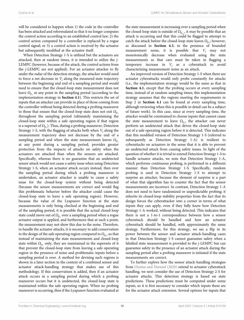
sampling periods. The first study involves an attack monitoringstrategy that involves checking whether the closed-loop state isoverall driven toward the origin over a sampling period (if it isnot, a possibility of an attack will be flagged). We implementattacks at 0.4 h; sensor attacks are implemented such that themeasurement received by the sensor at 0.4 h would be faulty, andan actuator attack would be implemented by replacing the inputcomputed for the time period between 0.4 and 0.41 h with analternative input. When no attack occurs in the sampling periodfollowing 0.4 h of operation, the Lyapunov function evaluated atthe actual state and at the state measurement decreases over thesubsequent sampling period, as shown in Figures 1, 2.

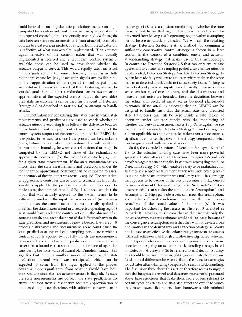
If instead we consider the case where only a rogue actuatoroutput with the form u = 0.5 kmol/m3 is provided to the processfor a sampling period after 0.4 h of operation, Figures 1, 2 showthat the Lyapunov function profile increases over one samplingperiod after the attack policy is applied, when the Lyapunovfunction is evaluated for both the actual state and the measuredstate, and thus, this single attack event would be flagged by theselected monitoring methodology. Consider now the case whereonly a false state measurement for reactant concentration, withthe form x1 + 0.5 kmol/m3, is continuously provided to thecontroller after 0.4 h of operation. This false sensormeasurement causes the Lyapunov function value to decreasealong the measurement trajectory, as can be seen in Figure 2,showing that this attack would not be detected by the strategy.However, it also decreases along the actual closed-loop statetrajectory in this case (Figure 1) so that no safety issueswould occur in this sampling period. This is thus a case whenindividual attacks would either be flagged over the subsequentsampling period or would not drive the closed-loop state toward

the boundary of the safe operating region over that samplingperiod. Due to the large (order-of-magnitude) difference in thevalue of V1 evaluated along the measured state trajectory betweenthe case that the sensor attack is applied and that no attack occurs,as shown in Figure 1, it could be argued that this type of attackcould be flagged by the steep jump in V1 between the times priorto the sensor attack that occurs at 0.4 and 0.4 h. However, becausewe assumed that the method for checking V1 was not put onlineuntil 0.4 h, we assume that it does not have a record of the priorvalue of V1 so that we can focus on the trends in this singlesampling period after the attacks.

We now consider two scenarios involving the combinations ofsensor and actuator attacks. First, we combine the two attacks justdescribed (i.e., false measurements are continuously provided tothe controller and detection policies, which have the form x1 +0.5 kmol/m3, and rogue actuator outputs with the form u =0.5 kmol/m3 are provided directly to the actuators to replaceany inputs computed by the controller). This attack is applied tothe process after 0.4 h of operation and subsequently referred toas the “baseline” combined actuator and sensor attack because itis a straightforward extension of the two separate attack policies.In this case, the value of V1 increases along the measurementtrajectory and also increases for the actual closed-loop state sothat this attack would be flagged by the proposed policy. In somesense, the addition of the actuator attack made the fact that thesystemwas under some type of attack “more visible” to this detectionpolicy than in the sensor attack-only case (although the individualsensor attack was not causing the closed-loop state to move towardthe boundary of the safe operating region so that the lack of detectionof an attack in that case would not be considered problematic).

FIGURE 1 | Actual V1 profiles over one sampling period after 0.4 h ofoperation for the process example described above in the presence of noattacks (“None”), only actuator cyberattacks (“Actuator”), only sensor attacks(“Sensor”), the baseline combined actuator and sensor attacks(“Combined”), and the stealthy combined sensor and actuator attack(“Stealthy”). The plots for the actuator attack, baseline combined actuator andsensor attack, and stealthy sensor and actuator attack are overlaid due to allhaving the same input (the false actuator signal) over the sampling period.

FIGURE2 | V1 profiles evaluated using the statemeasurements over onesampling period after 0.4 h of operation for the process example describedabove in the presence of no attacks (“None”), only actuator cyberattacks(“Actuator”), only sensor attacks (“Sensor”), the baseline combinedactuator and sensor attacks (“Combined”), and the stealthy combined sensorand actuator attack (“Stealthy”). The plots for no attack and for the stealthycombined sensor and actuator attack are overlaid because the stealthy attackprovides the no-attack sensor trajectory to the detection device to evadedetection.




www.frontiersin.org


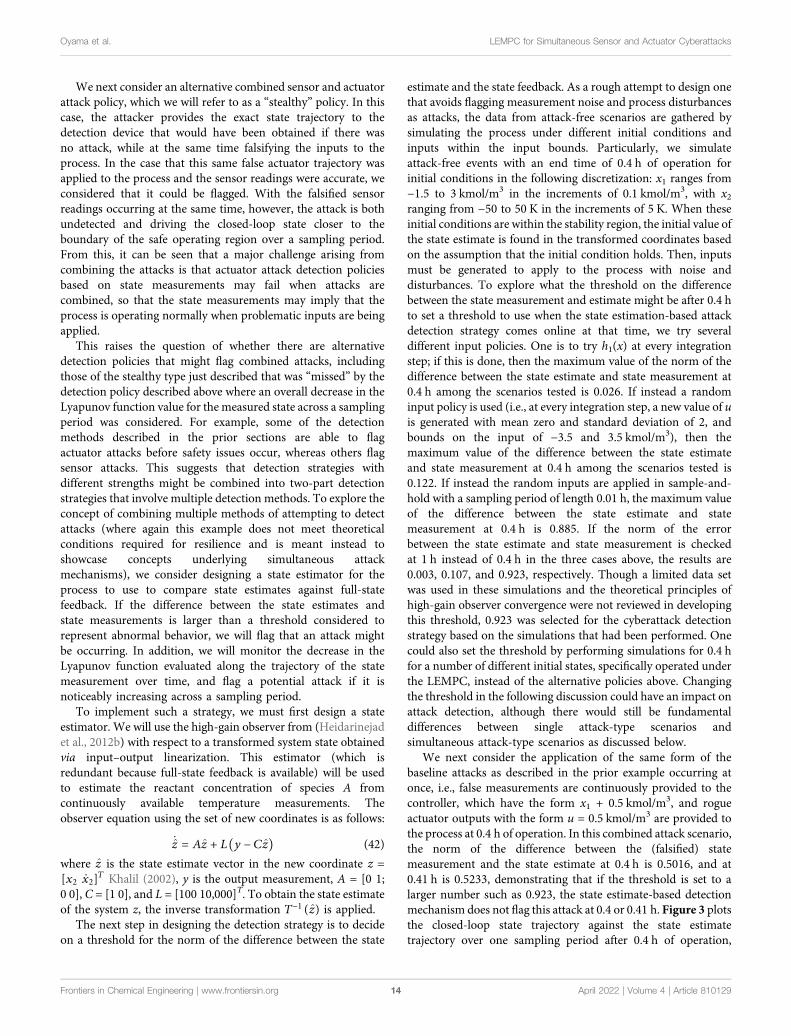
We next consider an alternative combined sensor and actuatorattack policy, which we will refer to as a “stealthy” policy. In thiscase, the attacker provides the exact state trajectory to thedetection device that would have been obtained if there wasno attack, while at the same time falsifying the inputs to theprocess. In the case that this same false actuator trajectory wasapplied to the process and the sensor readings were accurate, weconsidered that it could be flagged. With the falsified sensorreadings occurring at the same time, however, the attack is bothundetected and driving the closed-loop state closer to theboundary of the safe operating region over a sampling period.From this, it can be seen that a major challenge arising fromcombining the attacks is that actuator attack detection policiesbased on state measurements may fail when attacks arecombined, so that the state measurements may imply that theprocess is operating normally when problematic inputs are beingapplied.

This raises the question of whether there are alternativedetection policies that might flag combined attacks, includingthose of the stealthy type just described that was “missed” by thedetection policy described above where an overall decrease in theLyapunov function value for the measured state across a samplingperiod was considered. For example, some of the detectionmethods described in the prior sections are able to flagactuator attacks before safety issues occur, whereas others flagsensor attacks. This suggests that detection strategies withdifferent strengths might be combined into two-part detectionstrategies that involve multiple detection methods. To explore theconcept of combining multiple methods of attempting to detectattacks (where again this example does not meet theoreticalconditions required for resilience and is meant instead toshowcase concepts underlying simultaneous attackmechanisms), we consider designing a state estimator for theprocess to use to compare state estimates against full-statefeedback. If the difference between the state estimates andstate measurements is larger than a threshold considered torepresent abnormal behavior, we will flag that an attack mightbe occurring. In addition, we will monitor the decrease in theLyapunov function evaluated along the trajectory of the statemeasurement over time, and flag a potential attack if it isnoticeably increasing across a sampling period.

To implement such a strategy, we must first design a stateestimator. We will use the high-gain observer from (Heidarinejadet al., 2012b) with respect to a transformed system state obtainedvia input–output linearization. This estimator (which isredundant because full-state feedback is available) will be usedto estimate the reactant concentration of species A fromcontinuously available temperature measurements. Theobserver equation using the set of new coordinates is as follows:

_z � Az + L y − Cz( ) (42)where z is the state estimate vector in the new coordinate z �[x2 _x2]T Khalil (2002), y is the output measurement, A = [0 1;0 0], C = [1 0], and L = [100 10,000]T. To obtain the state estimateof the system z, the inverse transformation T−1(z) is applied.

The next step in designing the detection strategy is to decideon a threshold for the norm of the difference between the state

estimate and the state feedback. As a rough attempt to design onethat avoids flagging measurement noise and process disturbancesas attacks, the data from attack-free scenarios are gathered bysimulating the process under different initial conditions andinputs within the input bounds. Particularly, we simulateattack-free events with an end time of 0.4 h of operation forinitial conditions in the following discretization: x1 ranges from−1.5 to 3 kmol/m3 in the increments of 0.1 kmol/m3, with x2ranging from −50 to 50 K in the increments of 5 K. When theseinitial conditions are within the stability region, the initial value ofthe state estimate is found in the transformed coordinates basedon the assumption that the initial condition holds. Then, inputsmust be generated to apply to the process with noise anddisturbances. To explore what the threshold on the differencebetween the state measurement and estimate might be after 0.4 hto set a threshold to use when the state estimation-based attackdetection strategy comes online at that time, we try severaldifferent input policies. One is to try h1(x) at every integrationstep; if this is done, then the maximum value of the norm of thedifference between the state estimate and state measurement at0.4 h among the scenarios tested is 0.026. If instead a randominput policy is used (i.e., at every integration step, a new value of uis generated with mean zero and standard deviation of 2, andbounds on the input of −3.5 and 3.5 kmol/m3), then themaximum value of the difference between the state estimateand state measurement at 0.4 h among the scenarios tested is0.122. If instead the random inputs are applied in sample-and-hold with a sampling period of length 0.01 h, the maximum valueof the difference between the state estimate and statemeasurement at 0.4 h is 0.885. If the norm of the errorbetween the state estimate and state measurement is checkedat 1 h instead of 0.4 h in the three cases above, the results are0.003, 0.107, and 0.923, respectively. Though a limited data setwas used in these simulations and the theoretical principles ofhigh-gain observer convergence were not reviewed in developingthis threshold, 0.923 was selected for the cyberattack detectionstrategy based on the simulations that had been performed. Onecould also set the threshold by performing simulations for 0.4 hfor a number of different initial states, specifically operated underthe LEMPC, instead of the alternative policies above. Changingthe threshold in the following discussion could have an impact onattack detection, although there would still be fundamentaldifferences between single attack-type scenarios andsimultaneous attack-type scenarios as discussed below.

We next consider the application of the same form of thebaseline attacks as described in the prior example occurring atonce, i.e., false measurements are continuously provided to thecontroller, which have the form x1 + 0.5 kmol/m3, and rogueactuator outputs with the form u = 0.5 kmol/m3 are provided tothe process at 0.4 h of operation. In this combined attack scenario,the norm of the difference between the (falsified) statemeasurement and the state estimate at 0.4 h is 0.5016, and at0.41 h is 0.5233, demonstrating that if the threshold is set to alarger number such as 0.923, the state estimate-based detectionmechanism does not flag this attack at 0.4 or 0.41 h. Figure 3 plotsthe closed-loop state trajectory against the state estimatetrajectory over one sampling period after 0.4 h of operation,




www.frontiersin.org


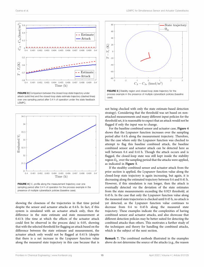
showing the closeness of the trajectories in that time perioddespite the sensor and actuator attacks at 0.4 h. In fact, if thissystem is simulated with an actuator attack only, then thedifference in the state estimate and state measurement at0.41 h (the time at which the effects of the actuator attackcould first be observed in the process data) is 0.05, showingthat with the selected threshold for flagging an attack based on thedifference between the state estimate and measurement, theactuator attack only would not be flagged at 0.41 h (despitethat there is a net increase in the Lyapunov function valuealong the measured state trajectory in this case because that is

not being checked with only the state estimate-based detectionstrategy). Considering that the threshold was set based on non-attacked measurements and many different input policies for thethreshold set, it is reasonable to expect that an attack would not beflagged if only the input was to change.

For the baseline combined sensor and actuator case, Figure 4shows that the Lyapunov function increases over the samplingperiod after 0.4 h along the measurement trajectory. Therefore,like the case where only the Lyapunov function was checked toattempt to flag this baseline combined attack, the baselinecombined sensor and actuator attack can be detected here aswell between 0.4 and 0.41 h. Though the attack occurs and isflagged, the closed-loop state was still kept inside the stabilityregionΩρ1 over the sampling period that the attacks were applied,as indicated in Figure 5.

If the stealthy combined sensor and actuator attack from theprior section is applied, the Lyapunov function value along theclosed-loop state trajectory is again increasing, but again, it isdecreasing along the estimated trajectory between 0.4 and 0.41 h.However, if this simulation is run longer, then the attack iseventually detected via the deviation of the state estimatesfrom the state measurements exceeding the 0.923 threshold, at0.45 h. In the case that only the Lyapunov function value alongthe measured state trajectories is checked until 0.45 h, no attack isyet detected, as the Lyapunov function value continues todecrease from 0.4 to 0.45 h along the measured statetrajectory. These examples indicate the complexities of havingcombined sensor and actuator attacks, and also showcase thatdifferent detection policies may be better suited for detecting thecombined attacks than others. This motivates a further study ofthe techniques and theory for handling the combined attacks,which is the subject of the next section.

Remark 7. The combined methods illustrated in the examplesabove do not determine the source of the attacks (e.g., the reason

FIGURE 3 |Comparison between the closed-loop state trajectory underattack (solid line) and the closed-loop state estimate trajectory (dashed lines)over one sampling period after 0.4 h of operation under the state feedbackLEMPC.

FIGURE 4 | V1 profile along the measurement trajectory over onesampling period after 0.4 h of operation for the process example in thepresence of multiple cyberattack policies (baseline case).

FIGURE 5 | Stability region and closed-loop state trajectory for theprocess example in the presence of multiple cyberattack policies (baselinecase).




www.frontiersin.org


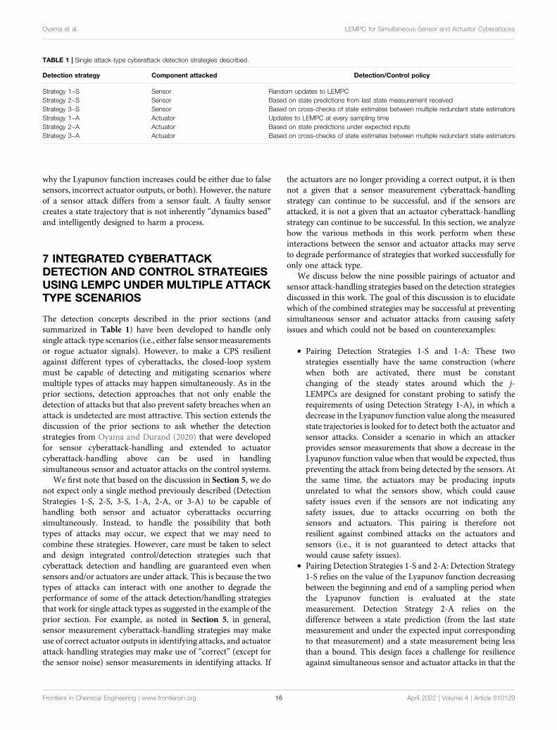
why the Lyapunov function increases could be either due to falsesensors, incorrect actuator outputs, or both). However, the natureof a sensor attack differs from a sensor fault. A faulty sensorcreates a state trajectory that is not inherently “dynamics based”and intelligently designed to harm a process.

7 INTEGRATED CYBERATTACKDETECTION AND CONTROL STRATEGIESUSING LEMPC UNDER MULTIPLE ATTACKTYPE SCENARIOS

The detection concepts described in the prior sections (andsummarized in Table 1) have been developed to handle onlysingle attack-type scenarios (i.e., either false sensor measurementsor rogue actuator signals). However, to make a CPS resilientagainst different types of cyberattacks, the closed-loop systemmust be capable of detecting and mitigating scenarios wheremultiple types of attacks may happen simultaneously. As in theprior sections, detection approaches that not only enable thedetection of attacks but that also prevent safety breaches when anattack is undetected are most attractive. This section extends thediscussion of the prior sections to ask whether the detectionstrategies from Oyama and Durand (2020) that were developedfor sensor cyberattack-handling and extended to actuatorcyberattack-handling above can be used in handlingsimultaneous sensor and actuator attacks on the control systems.

We first note that based on the discussion in Section 5, we donot expect only a single method previously described (DetectionStrategies 1-S, 2-S, 3-S, 1-A, 2-A, or 3-A) to be capable ofhandling both sensor and actuator cyberattacks occurringsimultaneously. Instead, to handle the possibility that bothtypes of attacks may occur, we expect that we may need tocombine these strategies. However, care must be taken to selectand design integrated control/detection strategies such thatcyberattack detection and handling are guaranteed even whensensors and/or actuators are under attack. This is because the twotypes of attacks can interact with one another to degrade theperformance of some of the attack detection/handling strategiesthat work for single attack types as suggested in the example of theprior section. For example, as noted in Section 5, in general,sensor measurement cyberattack-handling strategies may makeuse of correct actuator outputs in identifying attacks, and actuatorattack-handling strategies may make use of “correct” (except forthe sensor noise) sensor measurements in identifying attacks. If

the actuators are no longer providing a correct output, it is thennot a given that a sensor measurement cyberattack-handlingstrategy can continue to be successful, and if the sensors areattacked, it is not a given that an actuator cyberattack-handlingstrategy can continue to be successful. In this section, we analyzehow the various methods in this work perform when theseinteractions between the sensor and actuator attacks may serveto degrade performance of strategies that worked successfully foronly one attack type.

We discuss below the nine possible pairings of actuator andsensor attack-handling strategies based on the detection strategiesdiscussed in this work. The goal of this discussion is to elucidatewhich of the combined strategies may be successful at preventingsimultaneous sensor and actuator attacks from causing safetyissues and which could not be based on counterexamples:

• Pairing Detection Strategies 1-S and 1-A: These twostrategies essentially have the same construction (wherewhen both are activated, there must be constantchanging of the steady states around which the j-LEMPCs are designed for constant probing to satisfy therequirements of using Detection Strategy 1-A), in which adecrease in the Lyapunov function value along the measuredstate trajectories is looked for to detect both the actuator andsensor attacks. Consider a scenario in which an attackerprovides sensor measurements that show a decrease in theLyapunov function value when that would be expected, thuspreventing the attack from being detected by the sensors. Atthe same time, the actuators may be producing inputsunrelated to what the sensors show, which could causesafety issues even if the sensors are not indicating anysafety issues, due to attacks occurring on both thesensors and actuators. This pairing is therefore notresilient against combined attacks on the actuators andsensors (i.e., it is not guaranteed to detect attacks thatwould cause safety issues).

• Pairing Detection Strategies 1-S and 2-A: Detection Strategy1-S relies on the value of the Lyapunov function decreasingbetween the beginning and end of a sampling period whenthe Lyapunov function is evaluated at the statemeasurement. Detection Strategy 2-A relies on thedifference between a state prediction (from the last statemeasurement and under the expected input correspondingto that measurement) and a state measurement being lessthan a bound. This design faces a challenge for resilienceagainst simultaneous sensor and actuator attacks in that the

TABLE 1 | Single attack-type cyberattack detection strategies described.

Detection strategy Component attacked Detection/Control policy

Strategy 1−S Sensor Random updates to LEMPCStrategy 2−S Sensor Based on state predictions from last state measurement receivedStrategy 3−S Sensor Based on cross-checks of state estimates between multiple redundant state estimatorsStrategy 1−A Actuator Updates to LEMPC at every sampling timeStrategy 2−A Actuator Based on state predictions under expected inputsStrategy 3−A Actuator Based on cross-checks of state estimates between multiple redundant state estimators




www.frontiersin.org


detection strategies for both types of policies depend on thestate measurements. Since the state measurements here arefalsified, this gives room for any actuator signal to beutilized, and then the sensors to provide readings thatsuggest that the Lyapunov function is decreasing and thatthe prediction error is within a bound. Thus, in this strategy,because there is no way to cross-check whether the sensormeasurements are correct when there is also an actuatorattack, safety is not guaranteed when there are undetectedsimultaneous attacks.

• Pairing Detection Strategies 1-S and 3-A: Detection Strategy1-S relies on the state measurement creating a decrease inthe Lyapunov function, while Detection Strategy 3-A relieson redundant state estimates being sufficiently close to oneanother. If Detection Strategy 1-S is not constantly activated(i.e., there is no continuous probing), then becauseDetection Strategy 3-A may not be guaranteed to detectactuator attacks and Detection Strategy 1-S may not detectthem between probing times as described in Section 5, thisstrategy may not be resilient against actuator attacks (andthus also may not be against simultaneous actuator andsensor attacks). However, a slight modification to thestrategy to achieve constant probing under DetectionStrategy 1-S, forming the pairing of Detection Strategies3-S and 1-A (because Detection Strategies 3-A and 3-S areequivalent in how they are performed) is resilient againstsimultaneous sensor and actuator attacks, as is furtherdiscussed below. If instead of probing, Ωρ1 is designed tobe a sufficiently conservative subset of a safe operatingregion, then it could be checked whether at any time, thestate measurement leavesΩρ1 to flag the attacks; this strategywould also follow similarly to the strategy for detectingattacks using the combination of Detection Strategies 3-Sand 1-A for which a proof is provided in a subsequentsection.

• Pairing Detection Strategies 2-S and 1-A: This strategy facessimilar issues to the combination of Detection Strategies 1-Sand 2-A above. Specifically, these strategies again utilizestate measurements only to flag attacks, allowing rogueactuator inputs to be applied at the same time as falsestate measurements without allowing the attacks to beflagged.

• Pairing Detection Strategies 2-S and 2-A: This is a casewhere only state measurements are being used to flagattacks, so like other methods above where this isinsufficient to prevent the masking of rogue actuatortrajectories by false sensor measurements, this strategy isalso not resilient against attacks.

• Pairing Detection Strategies 2-S and 3-A: Detection Strategy2-S is based on the expected difference between statepredictions and actual states, and Detection Strategy 3-Ais based on checking the difference between multipleredundant state estimates. If the threshold for DetectionStrategy 2-S is redesigned (forming a pairing that we term asthe combination of Detection Strategies 2-A and 3-S belowsince the threshold redesign must account for actuatorattacks as described for Detection Strategy 2-A above to

avoid false alarms), the strategy would be resilient tosimultaneous actuator and sensor attacks. This is furtherdetailed in the subsequent sections (although it requires thatat least one state estimator is not impacted by the attacks).

• Pairing Detection Strategies 3-S and 1-A: This detectionstrategy can be made resilient against simultaneous actuatorand sensor attacks and receives further attention in thefollowing sections to demonstrate and discuss this (thoughat least one state estimator cannot be impacted by theattacks).

• Pairing Detection Strategies 3-S and 2-A: This strategy canbe made resilient for adequate thresholds on the stateprediction and state estimate-based detection metrics andwill be further detailed below.

• Pairing Detection Strategies 3-S and 3-A: This strategy facesthe challenge that it may not enable actuator attacks to bedetected because both Detection Strategy 3-S and DetectionStrategy 3-A are dependent only on state estimates, whichmay not reveal incorrect inputs as discussed in Section 5.Therefore, it would not be resilient for a case when actuatorand sensor attacks could both occur if the redundantobserver threshold holds regardless of the applied input.

The above discussion highlights that to handle both the sensorand actuator attacks, a combination strategy cannot be based onsensor measurements alone. In the following sections, we detailhow the combination strategies using Detection Strategies 3-Sand 1-A, and 3-S and 2-A, can be made resilient againstsimultaneous sensor and actuator attacks in the sense that, aslong as at least one state estimate is not impacted by a false sensormeasurement attack, the closed-loop state is always maintainedwithin a safe operating region if attacks are undetected, even ifboth attack types occur at once. We note that the assumptionsthat the detectors are intact (e.g., that at least one estimator is notimpacted by false sensor measurements or that a state predictionerror-based metric is evaluated against its threshold) implies thatother information technology (IT)-based defenses at the plant aresuccessful, indicating that the role of these strategies at this stageof development is not in replacing IT-based defenses but inproviding extra layers of protection if there are concerns thatthe attacks could reach the controller itself (while leaving somesensor measurements and detectors uncompromised).

7.1 Simultaneous Sensor and ActuatorAttack-Handling via Detection Strategies3-S and 1-A: Formulation andImplementationIn the spirit of the individual strategies Detection Strategy 3-S andDetection Strategy 1-A, a combined policy (to be termedDetection Strategy 1/3) can be developed that uses redundantstate estimates to check for sensor attacks (assuming that at leastone of the estimates is not impacted by any attack), and also usesdifferent LEMPCs at every sampling time that are designedaround different steady-states but contained within a subset ofa safe operating region Ωρsafe (the subsets are called Ωρi ⊂ Ωρsafe).Under sufficient conditions (which will be clarified in the next




www.frontiersin.org


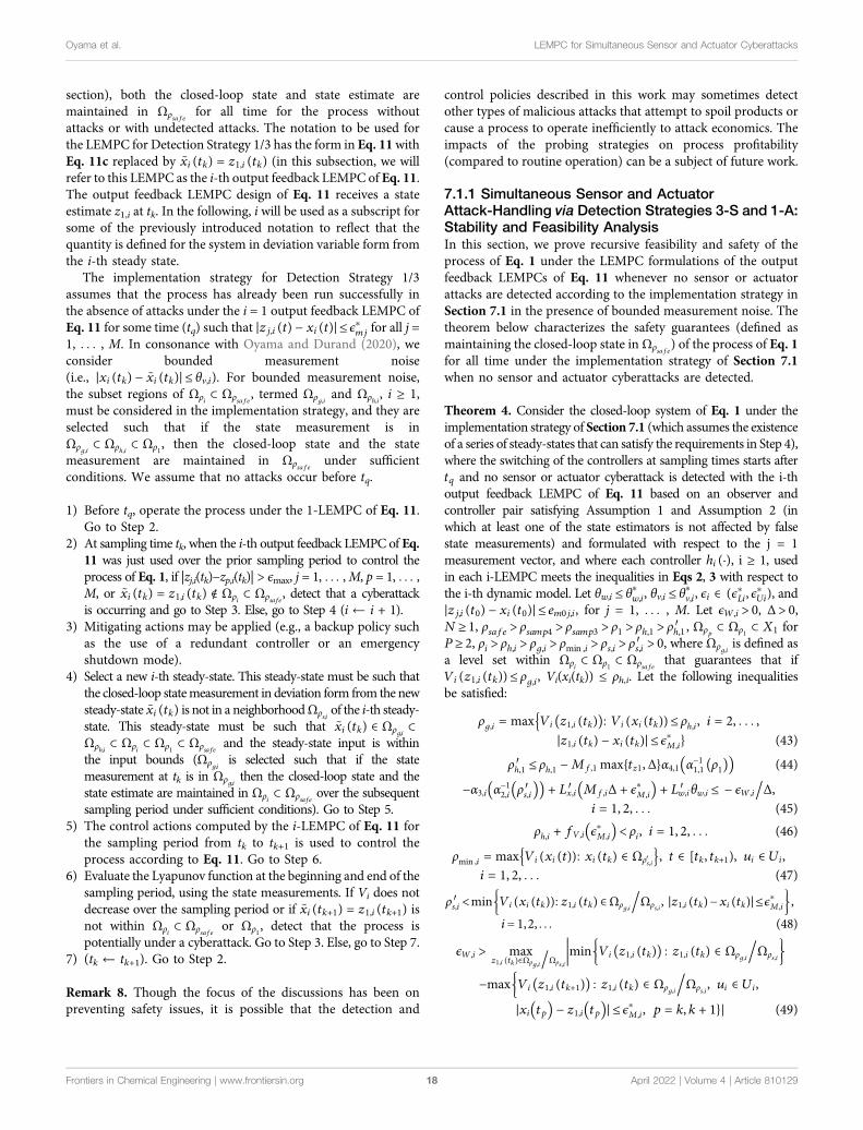
section), both the closed-loop state and state estimate aremaintained in Ωρsafe for all time for the process withoutattacks or with undetected attacks. The notation to be used forthe LEMPC for Detection Strategy 1/3 has the form in Eq. 11withEq. 11c replaced by ~xi(tk) � z1,i(tk) (in this subsection, we willrefer to this LEMPC as the i-th output feedback LEMPC of Eq. 11.The output feedback LEMPC design of Eq. 11 receives a stateestimate z1,i at tk. In the following, i will be used as a subscript forsome of the previously introduced notation to reflect that thequantity is defined for the system in deviation variable form fromthe i-th steady state.

The implementation strategy for Detection Strategy 1/3assumes that the process has already been run successfully inthe absence of attacks under the i = 1 output feedback LEMPC ofEq. 11 for some time (tq) such that |zj,i(t) − xi(t)|≤ ϵpmj for all j =1, . . . , M. In consonance with Oyama and Durand (2020), weconsider bounded measurement noise(i.e., |xi(tk) − ~xi(tk)|≤ θv,i). For bounded measurement noise,the subset regions of Ωρi ⊂ Ωρsafe, termed Ωρg,i and Ωρh,i, i ≥ 1,must be considered in the implementation strategy, and they areselected such that if the state measurement is inΩρg,i ⊂ Ωρh,i ⊂ Ωρ1, then the closed-loop state and the statemeasurement are maintained in Ωρsafe under sufficientconditions. We assume that no attacks occur before tq.

1) Before tq, operate the process under the 1-LEMPC of Eq. 11.Go to Step 2.

2) At sampling time tk, when the i-th output feedback LEMPC of Eq.11 was just used over the prior sampling period to control theprocess of Eq. 1, if |zj,i(tk)−zp,i(tk)| > ϵmax, j = 1, . . . ,M, p = 1, . . . ,M, or ~xi(tk) � z1,i(tk) ∉ Ωρi ⊂ Ωρsafe, detect that a cyberattackis occurring and go to Step 3. Else, go to Step 4 (i ← i + 1).

3) Mitigating actions may be applied (e.g., a backup policy suchas the use of a redundant controller or an emergencyshutdown mode).

4) Select a new i-th steady-state. This steady-state must be such thatthe closed-loop statemeasurement in deviation form from the newsteady-state ~xi(tk) is not in a neighborhoodΩρs,i of the i-th steady-state. This steady-state must be such that ~xi(tk) ∈ Ωρg,i ⊂Ωρh,i ⊂ Ωρi ⊂ Ωρ1 ⊂ Ωρsafe and the steady-state input is withinthe input bounds (Ωρg,i is selected such that if the statemeasurement at tk is in Ωρg,i then the closed-loop state and thestate estimate are maintained in Ωρi ⊂ Ωρsafe over the subsequentsampling period under sufficient conditions). Go to Step 5.

5) The control actions computed by the i-LEMPC of Eq. 11 forthe sampling period from tk to tk+1 is used to control theprocess according to Eq. 11. Go to Step 6.

6) Evaluate the Lyapunov function at the beginning and end of thesampling period, using the state measurements. If Vi does notdecrease over the sampling period or if ~xi(tk+1) � z1,i(tk+1) isnot within Ωρi ⊂ Ωρsafe or Ωρ1, detect that the process ispotentially under a cyberattack. Go to Step 3. Else, go to Step 7.

7) (tk ← tk+1). Go to Step 2.

Remark 8. Though the focus of the discussions has been onpreventing safety issues, it is possible that the detection and

control policies described in this work may sometimes detectother types of malicious attacks that attempt to spoil products orcause a process to operate inefficiently to attack economics. Theimpacts of the probing strategies on process profitability(compared to routine operation) can be a subject of future work.

7.1.1 Simultaneous Sensor and ActuatorAttack-Handling via Detection Strategies 3-S and 1-A:Stability and Feasibility AnalysisIn this section, we prove recursive feasibility and safety of theprocess of Eq. 1 under the LEMPC formulations of the outputfeedback LEMPCs of Eq. 11 whenever no sensor or actuatorattacks are detected according to the implementation strategy inSection 7.1 in the presence of bounded measurement noise. Thetheorem below characterizes the safety guarantees (defined asmaintaining the closed-loop state inΩρsafe) of the process of Eq. 1for all time under the implementation strategy of Section 7.1when no sensor and actuator cyberattacks are detected.

Theorem 4. Consider the closed-loop system of Eq. 1 under theimplementation strategy of Section 7.1 (which assumes the existenceof a series of steady-states that can satisfy the requirements in Step 4),where the switching of the controllers at sampling times starts aftertq and no sensor or actuator cyberattack is detected with the i-thoutput feedback LEMPC of Eq. 11 based on an observer andcontroller pair satisfying Assumption 1 and Assumption 2 (inwhich at least one of the state estimators is not affected by falsestate measurements) and formulated with respect to the j = 1measurement vector, and where each controller hi(·), i ≥ 1, usedin each i-LEMPC meets the inequalities in Eqs 2, 3 with respect tothe i-th dynamic model. Let θw,i ≤ θpw,i, θv,i ≤ θpv,i, ϵi ∈ (ϵpLi, ϵpUi), and|zj,i(t0) − xi(t0)|≤ em0j,i, for j = 1, . . . , M. Let ϵW,i > 0, Δ> 0,N≥ 1, ρsafe > ρsamp4 > ρsamp3 > ρ1 > ρh,1 > ρh,1′ , Ωρp ⊂ Ωρ1 ⊂ X1 forP≥ 2, ρi > ρh,i > ρg,i > ρmin ,i > ρs,i > ρs,i′ > 0, where Ωρg,i is defined asa level set within Ωρi ⊂ Ωρ1 ⊂ Ωρsafe that guarantees that ifVi(z1,i(tk))≤ ρg,i, Vi(xi(tk)) ≤ ρh,i. Let the following inequalitiesbe satisfied:

ρg,i � max Vi z1,i tk( )( ): Vi xi tk( )( )≤ ρh,i, i � 2, . . . ,{|z1,i tk( ) − xi tk( )|≤ ϵpM,i} (43)

ρh,1′ ≤ ρh,1 −Mf,1 max tz1,Δ{ }α4,1 α−11,1 ρ1( )( ) (44)−α3,i α

−12,i ρs,i′( )( ) + Lx,i′ Mf,iΔ + ϵpM,i( ) + Lw,i′ θw,i ≤ − ϵW,i/Δ,

i � 1, 2, . . . (45)ρh,i + fV,i ϵpM,i( )< ρi, i � 1, 2, . . . (46)

ρmin ,i � max Vi xi t( )( ): xi tk( ) ∈ Ωρs,i′{ }, t ∈ tk, tk+1[ ), ui ∈ Ui,

i � 1, 2, . . . (47)ρs,i′ <min Vi xi tk( )( ): z1,i tk( ) ∈Ωρg,i/Ωρs,i , |z1,i tk( )−xi tk( )|≤ϵpM,i{ },

i� 1,2, . . . (48)ϵW,i > max

z1,i tk( )∈Ωρg,i/Ωρs,i

min Vi z1,i tk( )( ) : z1,i tk( ) ∈ Ωρg,i/Ωρs,i{ }∣∣∣∣∣∣∣

−max Vi z1,i tk+1( )( ) : z1,i tk( ) ∈ Ωρg,i/Ωρs,i, ui ∈ Ui,{|xi tp( ) − z1,i tp( )|≤ ϵpM,i, p � k, k + 1}| (49)




www.frontiersin.org


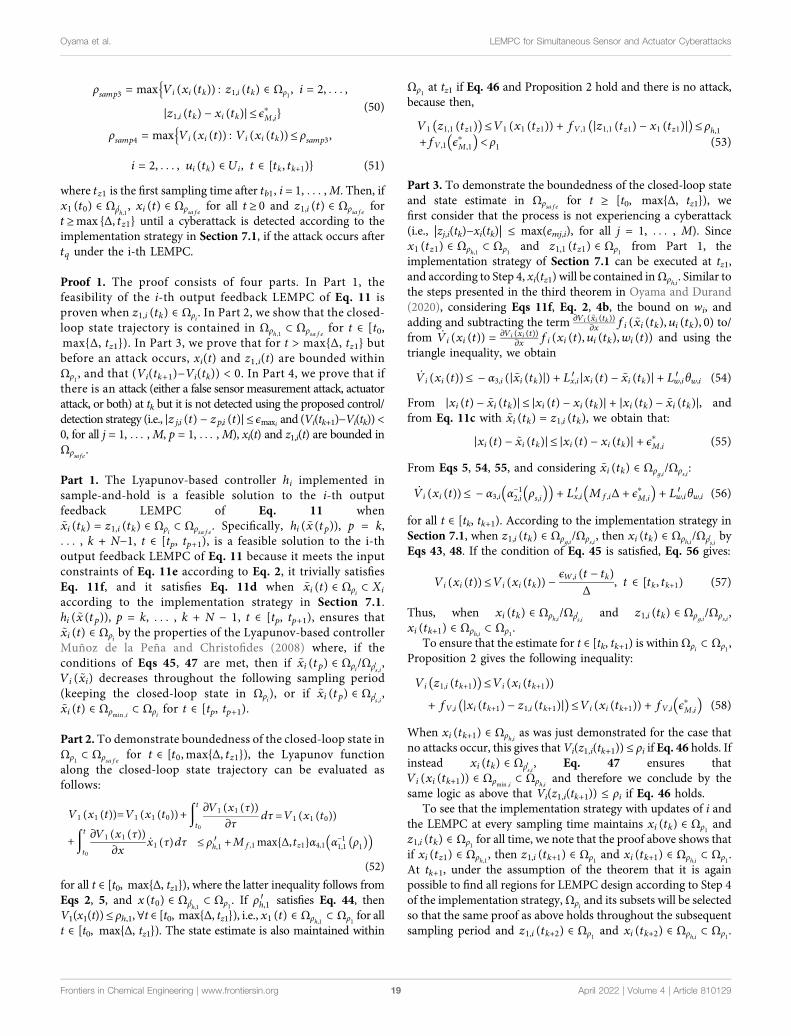
ρsamp3 � max Vi xi tk( )( ) : z1,i tk( ) ∈ Ωρ1, i � 2, . . . ,{|z1,i tk( ) − xi tk( )|≤ ϵpM,i} (50)

ρsamp4 � max Vi xi t( )( ) : Vi xi tk( )( )≤ ρsamp3,{i � 2, . . . , ui tk( ) ∈ Ui, t ∈ tk, tk+1[ )} (51)

where tz1 is the first sampling time after tb1, i = 1, . . . ,M. Then, ifx1(t0) ∈ Ωρh,1′ , xi(t) ∈ Ωρsafe for all t≥ 0 and z1,i(t) ∈ Ωρsafe fort≥max {Δ, tz1} until a cyberattack is detected according to theimplementation strategy in Section 7.1, if the attack occurs aftertq under the i-th LEMPC.

Proof 1. The proof consists of four parts. In Part 1, thefeasibility of the i-th output feedback LEMPC of Eq. 11 isproven when z1,i(tk) ∈ Ωρi. In Part 2, we show that the closed-loop state trajectory is contained in Ωρh,1 ⊂ Ωρsafe for t ∈ [t0,max{Δ, tz1}). In Part 3, we prove that for t > max{Δ, tz1} butbefore an attack occurs, xi(t) and z1,i(t) are bounded withinΩρ1, and that (Vi(tk+1)−Vi(tk)) < 0. In Part 4, we prove that ifthere is an attack (either a false sensor measurement attack, actuatorattack, or both) at tk but it is not detected using the proposed control/detection strategy (i.e., |zj,i(t) − zp,i(t)|≤ ϵmaxi and (Vi(tk+1)−Vi(tk))<0, for all j = 1, . . . ,M, p = 1, . . . ,M), xi(t) and z1,i(t) are bounded inΩρsafe.

Part 1. The Lyapunov-based controller hi implemented insample-and-hold is a feasible solution to the i-th outputfeedback LEMPC of Eq. 11 when~xi(tk) � z1,i(tk) ∈ Ωρi ⊂ Ωρsafe. Specifically, hi(~x(tp)), p = k,. . . , k + N−1, t ∈ [tp, tp+1), is a feasible solution to the i-thoutput feedback LEMPC of Eq. 11 because it meets the inputconstraints of Eq. 11e according to Eq. 2, it trivially satisfiesEq. 11f, and it satisfies Eq. 11d when ~xi(t) ∈ Ωρi ⊂ Xi

according to the implementation strategy in Section 7.1.hi(~x(tp)), p = k, . . . , k + N − 1, t ∈ [tp, tp+1), ensures that~xi(t) ∈ Ωρi by the properties of the Lyapunov-based controllerMuñoz de la Peña and Christofides (2008) where, if theconditions of Eqs 45, 47 are met, then if ~xi(tp) ∈ Ωρi/Ωρs,i′ ,Vi(~xi) decreases throughout the following sampling period(keeping the closed-loop state in Ωρi), or if ~xi(tp) ∈ Ωρs,i′ ,~xi(t) ∈ Ωρmin ,i

⊂ Ωρi for t ∈ [tp, tp+1).

Part 2. To demonstrate boundedness of the closed-loop state inΩρ1 ⊂ Ωρsafe for t ∈ [t0,max{Δ, tz1}), the Lyapunov functionalong the closed-loop state trajectory can be evaluated asfollows:

V1 x1 t( )( )�V1 x1 t0( )( )+∫t0

t zV1 x1 τ( )( )zτ

dτ �V1 x1 t0( )( )+∫

t0

t zV1 x1 τ( )( )zx

_x1 τ( )dτ ≤ ρh,1′ +Mf,1max Δ, tz1{ }α4,1 α−11,1 ρ1( )( )(52)

for all t ∈ [t0, max{Δ, tz1}), where the latter inequality follows fromEqs 2, 5, and x(t0) ∈ Ωρh,1′ ⊂ Ωρ1. If ρh,1′ satisfies Eq. 44, thenV1(x1(t))≤ ρh,1, ∀t ∈ [t0, max{Δ, tz1}), i.e., x1(t) ∈ Ωρh,1 ⊂ Ωρ1 for allt ∈ [t0, max{Δ, tz1}). The state estimate is also maintained within

Ωρ1 at tz1 if Eq. 46 and Proposition 2 hold and there is no attack,because then,

V1 z1,1 tz1( )( )≤V1 x1 tz1( )( ) + fV,1 |z1,1 tz1( ) − x1 tz1( )|( )≤ ρh,1+fV,1 ϵpM,1( )< ρ1 (53)

Part 3. To demonstrate the boundedness of the closed-loop stateand state estimate in Ωρsafe for t ≥ [t0, max{Δ, tz1}), wefirst consider that the process is not experiencing a cyberattack(i.e., |zj,i(tk)−xi(tk)| ≤ max(emj,i), for all j = 1, . . . , M). Sincex1(tz1) ∈ Ωρh,1 ⊂ Ωρ1 and z1,1(tz1) ∈ Ωρ1 from Part 1, theimplementation strategy of Section 7.1 can be executed at tz1,and according to Step 4, xi(tz1) will be contained inΩρh,i. Similar tothe steps presented in the third theorem in Oyama and Durand(2020), considering Eqs 11f, Eq. 2, 4b, the bound on wi, andadding and subtracting the term zVi(~xi(tk))

zx fi(~xi(tk), ui(tk), 0) to/from _Vi(xi(t)) � zVi(xi(t))

zx fi(xi(t), ui(tk), wi(t)) and using thetriangle inequality, we obtain

_Vi xi t( )( )≤ − α3,i |~xi tk( )|( ) + Lx,i′ |xi t( ) − ~xi tk( )| + Lw,i′ θw,i (54)From |xi(t) − ~xi(tk)|≤ |xi(t) − xi(tk)| + |xi(tk) − ~xi(tk)|, andfrom Eq. 11c with ~xi(tk) � z1,i(tk), we obtain that:

|xi t( ) − ~xi tk( )|≤ |xi t( ) − xi tk( )| + ϵpM,i (55)From Eqs 5, 54, 55, and considering ~xi(tk) ∈ Ωρg,i/Ωρs,i:

_Vi xi t( )( )≤ − α3,i α−12,i ρs,i( )( ) + Lx,i′ Mf,iΔ + ϵpM,i( ) + Lw,i′ θw,i (56)

for all t ∈ [tk, tk+1). According to the implementation strategy inSection 7.1, when z1,i(tk) ∈ Ωρg,i/Ωρs,i, then xi(tk) ∈ Ωρh,i/Ωρs,i′ byEqs 43, 48. If the condition of Eq. 45 is satisfied, Eq. 56 gives:

Vi xi t( )( )≤Vi xi tk( )( ) − ϵW,i t − tk( )Δ , t ∈ tk, tk+1[ ) (57)

Thus, when xi(tk) ∈ Ωρh,i/Ωρs,i′ and z1,i(tk) ∈ Ωρg,i/Ωρs,i,xi(tk+1) ∈ Ωρh,i ⊂ Ωρ1.

To ensure that the estimate for t ∈ [tk, tk+1) is withinΩρi ⊂ Ωρ1,Proposition 2 gives the following inequality:

Vi z1,i tk+1( )( )≤Vi xi tk+1( )( )+ fV,i |xi tk+1( ) − z1,i tk+1( )|( )≤Vi xi tk+1( )( ) + fV,i ϵpM,i( ) (58)

When xi(tk+1) ∈ Ωρh,i as was just demonstrated for the case thatno attacks occur, this gives thatVi(z1,i(tk+1)) ≤ ρi if Eq. 46 holds. Ifinstead xi(tk) ∈ Ωρs,i′ , Eq. 47 ensures thatVi(xi(tk+1)) ∈ Ωρmin ,i

⊂ Ωρh,i and therefore we conclude by thesame logic as above that Vi(z1,i(tk+1)) ≤ ρi if Eq. 46 holds.

To see that the implementation strategy with updates of i andthe LEMPC at every sampling time maintains xi(tk) ∈ Ωρ1 andz1,i(tk) ∈ Ωρ1 for all time, we note that the proof above shows thatif xi(tz1) ∈ Ωρh,1, then z1,i(tk+1) ∈ Ωρ1 and xi(tk+1) ∈ Ωρh,i ⊂ Ωρ1.At tk+1, under the assumption of the theorem that it is againpossible to find all regions for LEMPC design according to Step 4of the implementation strategy,Ωρi and its subsets will be selectedso that the same proof as above holds throughout the subsequentsampling period and z1,i(tk+2) ∈ Ωρ1 and xi(tk+2) ∈ Ωρh,i ⊂ Ωρ1.




www.frontiersin.org


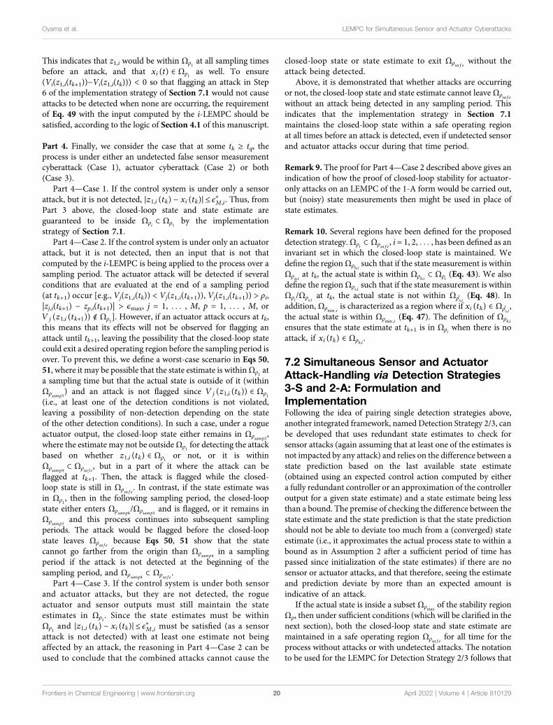
This indicates that z1,i would be within Ωρ1 at all sampling timesbefore an attack, and that xi(t) ∈ Ωρ1 as well. To ensure(Vi(z1,i(tk+1))−Vi(z1,i(tk))) < 0 so that flagging an attack in Step6 of the implementation strategy of Section 7.1 would not causeattacks to be detected when none are occurring, the requirementof Eq. 49 with the input computed by the i-LEMPC should besatisfied, according to the logic of Section 4.1 of this manuscript.

Part 4. Finally, we consider the case that at some tk ≥ tq, theprocess is under either an undetected false sensor measurementcyberattack (Case 1), actuator cyberattack (Case 2) or both(Case 3).

Part 4—Case 1. If the control system is under only a sensorattack, but it is not detected, |z1,i(tk) − xi(tk)|≤ ϵpM,i. Thus, fromPart 3 above, the closed-loop state and state estimate areguaranteed to be inside Ωρi ⊂ Ωρ1 by the implementationstrategy of Section 7.1.

Part 4—Case 2. If the control system is under only an actuatorattack, but it is not detected, then an input that is not thatcomputed by the i-LEMPC is being applied to the process over asampling period. The actuator attack will be detected if severalconditions that are evaluated at the end of a sampling period(at tk+1) occur [e.g., Vj(z1,i(tk)) < Vj(z1,i(tk+1)), Vj(z1,i(tk+1)) > ρi,|zj,i(tk+1) − zp,i(tk+1)| > ϵmax, j = 1, . . . , M, p = 1, . . . , M, orVj(z1,i(tk+1)) ∉ Ωρ1]. However, if an actuator attack occurs at tk,this means that its effects will not be observed for flagging anattack until tk+1, leaving the possibility that the closed-loop statecould exit a desired operating region before the sampling period isover. To prevent this, we define a worst-case scenario in Eqs 50,51, where it may be possible that the state estimate is withinΩρ1 ata sampling time but that the actual state is outside of it (withinΩρsamp3

) and an attack is not flagged since Vj(z1,i(tk)) ∈ Ωρ1(i.e., at least one of the detection conditions is not violated,leaving a possibility of non-detection depending on the stateof the other detection conditions). In such a case, under a rogueactuator output, the closed-loop state either remains in Ωρsamp3

,where the estimate may not be outsideΩρ1 for detecting the attackbased on whether z1,i(tk) ∈ Ωρ1 or not, or it is withinΩρsamp4

⊂ Ωρsafe, but in a part of it where the attack can beflagged at tk+1. Then, the attack is flagged while the closed-loop state is still in Ωρsafe. In contrast, if the state estimate wasin Ωρ1, then in the following sampling period, the closed-loopstate either enters Ωρsamp4

/Ωρsamp3and is flagged, or it remains in

Ωρsamp3and this process continues into subsequent sampling

periods. The attack would be flagged before the closed-loopstate leaves Ωρsafe because Eqs 50, 51 show that the statecannot go farther from the origin than Ωρsamp4

in a samplingperiod if the attack is not detected at the beginning of thesampling period, and Ωρsamp4

⊂ Ωρsafe.Part 4—Case 3. If the control system is under both sensor

and actuator attacks, but they are not detected, the rogueactuator and sensor outputs must still maintain the stateestimates in Ωρ1. Since the state estimates must be withinΩρ1 and |z1,i(tk) − xi(tk)|≤ ϵpM,i must be satisfied (as a sensorattack is not detected) with at least one estimate not beingaffected by an attack, the reasoning in Part 4—Case 2 can beused to conclude that the combined attacks cannot cause the

closed-loop state or state estimate to exit Ωρsafe without theattack being detected.

Above, it is demonstrated that whether attacks are occurringor not, the closed-loop state and state estimate cannot leaveΩρsafewithout an attack being detected in any sampling period. Thisindicates that the implementation strategy in Section 7.1maintains the closed-loop state within a safe operating regionat all times before an attack is detected, even if undetected sensorand actuator attacks occur during that time period.

Remark 9. The proof for Part 4—Case 2 described above gives anindication of how the proof of closed-loop stability for actuator-only attacks on an LEMPC of the 1-A form would be carried out,but (noisy) state measurements then might be used in place ofstate estimates.

Remark 10. Several regions have been defined for the proposeddetection strategy.Ωρi ⊂ Ωρsafe, i = 1, 2, . . . , has been defined as aninvariant set in which the closed-loop state is maintained. Wedefine the regionΩρh,i such that if the state measurement is withinΩρg,i at tk, the actual state is within Ωρh,i ⊂ Ωρi (Eq. 43). We alsodefine the regionΩρs,i such that if the state measurement is withinΩρi/Ωρs,i at tk, the actual state is not within Ωρs,i′ (Eq. 48). Inaddition, Ωρmin ,i

is characterized as a region where if xi(tk) ∈ Ωρs,i′ ,the actual state is within Ωρmin ,i

(Eq. 47). The definition of Ωρh,iensures that the state estimate at tk+1 is in Ωρi when there is noattack, if xi(tk) ∈ Ωρh,i.

7.2 Simultaneous Sensor and ActuatorAttack-Handling via Detection Strategies3-S and 2-A: Formulation andImplementationFollowing the idea of pairing single detection strategies above,another integrated framework, named Detection Strategy 2/3, canbe developed that uses redundant state estimates to check forsensor attacks (again assuming that at least one of the estimates isnot impacted by any attack) and relies on the difference between astate prediction based on the last available state estimate(obtained using an expected control action computed by eithera fully redundant controller or an approximation of the controlleroutput for a given state estimate) and a state estimate being lessthan a bound. The premise of checking the difference between thestate estimate and the state prediction is that the state predictionshould not be able to deviate too much from a (converged) stateestimate (i.e., it approximates the actual process state to within abound as in Assumption 2 after a sufficient period of time haspassed since initialization of the state estimates) if there are nosensor or actuator attacks, and that therefore, seeing the estimateand prediction deviate by more than an expected amount isindicative of an attack.

If the actual state is inside a subset Ωρmaxof the stability region

Ωρ, then under sufficient conditions (which will be clarified in thenext section), both the closed-loop state and state estimate aremaintained in a safe operating region Ωρsafe for all time for theprocess without attacks or with undetected attacks. The notationto be used for the LEMPC for Detection Strategy 2/3 follows that




www.frontiersin.org


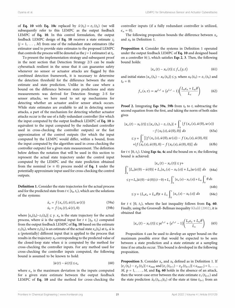
of Eq. 10 with Eq. 10c replaced by ~x(tk) � z1(tk) (we willsubsequently refer to this LEMPC as the output feedbackLEMPC of Eq. 10. In this control formulation, the outputfeedback LEMPC design of Eq. 10 receives a state estimate zj(j = 1, . . . , M) from one of the redundant state estimators (theestimator used to provide state estimates to the proposed LEMPCthat controls the process will be denoted as the j = 1 estimator) at tk.

To present the implementation strategy and subsequent proofin the next section that Detection Strategy 2/3 can be madecyberattack resilient in the sense that it can guarantee safetywhenever no sensor or actuator attacks are flagged by thiscombined detection framework, it is necessary to determinethe detection threshold for the difference between the stateestimate and state prediction. Unlike in the case where abound on the difference between state predictions and statemeasurements was derived for Detection Strategy 2-S forsensor attacks, we here need to set up mechanisms fordetecting whether an actuator and/or sensor attack occurs.While state estimates are available to aid in detecting sensorattacks, a part of the mechanism for detecting whether actuatorattacks occur is the use of a fully redundant controller (for whichthe input computed by the output feedback LEMPC of Eq. 10 isequivalent to the input computed by the redundant controllerused in cross-checking the controller outputs) or the fastapproximation of the control outputs (for which the inputcomputed by the LEMPC would differ, within a bound, fromthe input computed by the algorithm used in cross-checking thecontroller outputs) for a given state measurement. The definitionbelow defines the notation that will be used in this section torepresent the actual state trajectory under the control inputcomputed by the LEMPC and the state prediction obtainedfrom the nominal (w ≡ 0) process model of Eq. 1 under thepotentially approximate input used for cross-checking the controloutputs.

Definition 1. Consider the state trajectories for the actual processand for the predicted state from t ∈ [t0, t1), which are the solutionsof the systems:

_xa � f xa t( ), �u t( ), w t( )( ) (59a)_xb � f xb t( ), u t( ), 0( ) (59b)

where |xa(t0)−z1(t0)| ≤ γ. xa is the state trajectory for the actualprocess, where �u is the optimal input for t ∈ [t0, t1) computedfrom the output feedback LEMPC of Eq. 10 based on the estimatez1(t0), where z1(t0) is an estimate of the actual state xa(t0) at t0. u isa (potentially) different input that is applied to the process thatresults in the trajectory xb corresponding to the predicted value ofthe closed-loop state when u is computed by the method forcross-checking the controller inputs. For any method used forcross-checking the controller inputs computed, the followingbound is assumed to be known to hold:

|�u t( ) − u t( )|≤ ϵu (60)where ϵu is the maximum deviation in the inputs computedfor a given state estimate between the output feedbackLEMPC of Eq. 10 and the method for cross-checking the

controller inputs (if a fully redundant controller is utilized,ϵu = 0).

The following proposition bounds the difference between xaand xb in Definition 1.

Proposition 4. Consider the systems in Definition 1 operatedunder the output feedback LEMPC of Eq. 10 and designed basedon a controller h(·), which satisfies Eqs 2, 3. Then, the followingbound holds:

|xa t( ) − xb t( )|≤fu γ, t( ) (61)and initial states |xa(t0) − xb(t0)|≤ γ, where xb(t0) � z1(t0) andt0 = 0:

fu s, τ( ) ≔ seLxt + eLxt − 1( ) Luϵu + Lwθ

Lx( ) (62)

Proof 2. Integrating Eqs 59a, 59b from t0 to t, subtracting thesecond equation from the first, and taking the norm of both sidesgives

|xa t( ) − xb t( )|≤ |xa t0( ) − z1 t0( )| + ∫0

t |f xa s( ), �u 0( ), w s( )( )−f xb s( ), u 0( ), 0( )| ds (63a)

≤ γ + ∫0

t |f xa s( ), �u 0( ), w s( )( ) − f xb s( ), �u 0( ), 0( )|[+|f xb s( ), �u 0( ), 0( ) − f xb s( ), u 0( ), 0( )|] ds (63b)

for t ∈ [0, t1). Using Eqs 4a, 4c and the bound on w, the followingbound is achieved:

|xa t( ) − xb t( )|≤ γ+∫0

tLu|�u 0( ) − u 0( )| + Lx|xa s( ) − xb s( )| + Lw|w s( )|[ ] ds (64a)

≤γ+Lu|�u 0( )− u 0( )| t−0( )+Lx∫0

t |xa s( )−xb s( )|+Lw∫0

tθ ds

(64b)≤ γ + Luϵu + Lwθ( )t + Lx ∫

0

t |xa s( ) − xb s( )| ds (64c)

for t ∈ [0, t1), where the last inequality follows from Eq. 60.Finally, using the Gronwall–Bellman inequality Khalil (2002), it isobtained that

|xa t( ) − xb t( )|≤ γeLxt + eLxt − 1( ) Luϵu + Lwθ

Lx( ) (65)

Proposition 4 can be used to develop an upper bound on themaximum possible error that would be expected to be seenbetween a state prediction and a state estimate at a samplingtime if no attacks occur. This bound is developed in the followingproposition.

Proposition 5. Consider xa and xb defined as in Definition 1. If|zj(tk) − zp(tk)|< ϵmax and |zj(tk+1) − zp(tk+1)|< ϵmax, j = 1, . . . ,M, p = 1, . . . , M, and Eq. 60 holds in the absence of an attack,then the worst-case error between the state estimate z1(tk+1) andthe state prediction ~xb(tk+1|tk) of the state at time tk+1 from an




www.frontiersin.org


estimate obtained at time tk in the absence of an attack on theactuators or sensors is given by

|z1 tk+1( ) − ~xb tk+1|tk( )|≤ ϵpM + fu ϵpM,Δ( ) (66)

Proof 3. Using Proposition 3 and Proposition 4 along with Eq.32, we obtain

|z1 tk+1( )− ~xb tk+1|tk( )|≤ |z1 tk+1( )−xa tk+1( )|+ |xa tk+1( )− ~xb tk+1|tk( )|≤ϵpM +fu |xa tk( )−z1 tk( )|,Δ( )≤ϵpM +fu ϵpM,Δ( )

(67)Proposition 5 demonstrates that if an upper bound ]u ≥ ϵpM +

fu(ϵpM,Δ) is placed on |z1(tk+1) − ~xb(tk+1|tk)|, then a cyberattackcould be flagged if |z1(tk+1) − ~xb(tk+1|tk)|> ]u without creatingfalse alarms, as |z1(tk+1) − ~xb(tk+1|tk)| should never becomegreater than ]u if no attack is occurring according to the proofof the proposition.

We now describe the implementation strategy of DetectionStrategy 2/3, which assumes that the process has already been runsuccessfully in the absence of attacks under the output feedbackLEMPC of Eq. 10 for some time (tq) such that |zj(t) − x(t)|≤ ϵpmjfor all j = 1, . . . , M.

1) At sampling time tk, when the output feedback LEMPC of Eq.10 is used to control the process of Eq. 1, if |zj(tk)−zp(tk)| >ϵmax or |zj(tk−1)−zp(tk−1)| > ϵmax, j = 1, . . . ,M, p = 1, . . . ,M, or~x(tk) � z1(tk) ∉ Ωρ (where z1 is the state estimate used in theproposed LEMPC design that controls the process), detectthat a cyberattack is occurring and go to Step 2. If no attack isflagged, check whether |~x(tk|tk−1) − z1(tk)|> ]u (where]u ≥ ϵpM + fu(ϵpM,Δ)). If yes, flag that a cyberattack ishappening and go to Step 2. Else, go to Step 3.

2) Mitigating actions may be applied (e.g., a backup policy suchas the use of redundant controller or an emergency shutdownmode).

3) Control the process using the output feedback LEMPC of Eq.10. Go to Step 4.

4) (tk ← tk+1). Go to Step 1.

7.2.1 Simultaneous Sensor and ActuatorAttack-Handling via Detection Strategies 3-S and 2-A:Stability and Feasibility AnalysisIn this section, we prove recursive feasibility and stability of theprocess of Eq. 1 under the proposed output feedback LEMPC ofEq. 10 whenever no sensor or actuator attacks are detectedaccording to the implementation strategy in Section 7.2 in thepresence of bounded plant/model mismatch, controller cross-check error, and measurement noise. The following theoremcharacterizes the safety guarantees of the process of Eq. 1 forall time under the implementation strategy of Section 7.2 whensensor and actuator cyberattacks are not detected. As forDetection Strategy 1/3, because the actuator cyberattackswould not be detected according to the implementationstrategy in Section 7.2 until a sampling period after they hadoccurred (since they are being detected by their action on the stateestimates, which would not be obvious until they have had achance to impact the closed-loop state), it is necessary to define

supersets Ωρsamp3and Ωρsamp4

of Ωρ, but which are contained inΩρsafe, to set the size of Ωρ with respect to Ωρsafe to ensure that Ωρ

is defined in a sufficiently conservative fashion such that even ifthe closed-loop state is driven out ofΩρ, the closed-loop state willstill always be in Ωρsafe and the state estimate will go out of Ωρ

before the actual closed-loop state leaves Ωρsafe.

Theorem 5. Consider the closed-loop system of Eq. 1 underthe implementation strategy of Section 7.2, in which nosensor or actuator cyberattack is detected using theproposed output feedback LEMPC of Eq. 10 based on anobserver and controller pair satisfying Assumption 1 andAssumption 2 and formulated with respect to the i = 1measurement vector and a controller h(·) that meets Eqs 2,3. Let the conditions of Proposition 3 and Proposition 4 hold,and θw ≤ θpw, θv,i ≤ θ

pv,i, ϵi ∈ (ϵpLi, ϵpUi), and |zi(t0) − x(t0)|≤ em0i,

for i = 1, . . . , M. Also, let ϵW,1 > 0, Δ > 0, Ωρ ⊂ X, andρsafe > ρsamp4 > ρsamp3 > ρ> ρmax > ρ1,1 > ρe,1′ > ρmin ,1 > ρs,1 > 0, satisfy:ρe,1′ ≤ ρmax

−max fV fW ϵpM,Δ( )( ),Mf max tz1,Δ{ }α4 α−11 ρmax( )( ){ } (68)ρe,1′ ≤ ρ − fV fW ϵpM,Δ( )( ) − fV ϵpM( ) (69)

−α3 α−12 ρs,1( )( ) + Lx′ MfΔ + ϵpM( ) + Lw′ θw ≤ − ϵW,1/Δ (70)ρmin ,1 � max V x t + Δ( )( )|V x t( )( )≤ ρs,1{ } (71)

ρmin ,1 + fV fW ϵpM,Δ( )( )≤ ρ (72)ρmax + fV ϵpM( )≤ ρ (73)

ρsamp3 � max V x tk( )( ) : z1 tk( ) ∈ Ωρ, |z1 tk( ) − x tk( )|≤ ϵpM{ }(74)

ρsamp4 �max V x t( )( ) :V x tk( )( )≤ ρsamp3, u tk( ) ∈U, t ∈ tk, tk+1[ ){ }(75)

where tz1 is the first sampling time after tb1, and fv, fw, and fu

are defined as in Proposition 1, Proposition 2 (with thesubscripts dropped), and Proposition 4. Then, ifx(t0) ∈ Ωρe,1, x(t) ∈ Ωρmax

for all t≥ 0 and z1(th) ∈ Ωρ forth ≥max {Δ, tz1} until a cyberattack is detected according tothe implementation strategy in Section 7.2, if the attack occursafter tq.

Proof 4. The output feedback LEMPC of Eq. 10 has the sameform as in Oyama and Durand (2020). Therefore, in the absenceof attacks or in the presence of sensor attacks only, we obtain thesame results as in Oyama and Durand (2020). Specifically,feasibility follows when z1(tk) ∈ Ωρ as proven in Oyama andDurand (2020). Since z1(tk) ∉ Ωρ flags an attack according to theimplementation strategy of Section 7.2, there will not be a timebefore an attack is detected that z1(tk) ∉ Ωρ before an attack, sothat the problem would not be infeasible before an attack. Also asdemonstrated in Oyama andDurand (2020), the closed-loop statetrajectory is contained inΩρmax

for t ∈ [t0, max{Δ, tz1}), and beforean attack occurs when t ≥ max{Δ, tz1}, x(t) is bounded withinΩρmax

and z1(t) is bounded within Ωρ. Furthermore, it followsfrom Proposition 3 and Proposition 5 that the implementationstrategy of Section 7.2 will not detect measurement noise,




www.frontiersin.org


controller cross-check error, or bounded plant/model mismatchas attacks, such that there will be no false detections. It remains todemonstrate that if there is an attack at tk but it is not detectedusing the proposed methodology (i.e., | zi(tk)−zj(tk)| ≤ ϵmax,|zi(tk−1)−zj(tk−1)| ≤ ϵmax, for all i = 1, . . . , M, j = 1, . . . , M,~x(tk) � z1(tk) ∈ Ωρ, and |~x(tk|tk−1) − z1(tk)|≤ ]u), then z1(tk+1)and x(t), t ∈ [tk, tk+1), are bounded in Ωρsafe.

If the control system is under only a sensor attack, but it is notdetected, then under the conditions of Theorem 5, the closed-loop state remains inside Ωρmax

⊂ Ωρsafe and the state estimateremains within Ωρsafe under the implementation strategy ofSection 7.2, following Oyama and Durand (2020).

If the control system is under only an actuator attack, then viathe same steps as in the proof of Theorem 4 for Case 4—Part 2withΩρ1 replaced byΩρ, the attack will be detected before it drivesthe closed-loop state out of Ωρsafe. The same proof demonstratesthat when simultaneous sensor and actuator attacks occur, theclosed-loop state will not be driven out ofΩρsafe before an attack isdetected. Applying these proofs recursively indicates that underthis implementation strategy, an attack is detected before theclosed-loop state leaves Ωρsafe.

Remark 11. The proof for actuator-only attacks for Theorem 5described above gives an indication of how the proof of closed-loop stability for actuator-only attacks on an LEMPC of the 2-Aform would be carried out, but state measurements might then beused in place of state estimates, with the bound developed on thedifference between the state estimate and state prediction updatedto be between the measurement and prediction.

8 CYBERATTACK DISCOVERABILITY FORNONLINEAR SYSTEMS

The above sections reviewed a variety of cyberattack-handlingmechanisms that rely on specific detection strategies designed intandem with the controllers. None of those strategies, in themanner discussed, detects every attack, but some ensure thatsafety is maintained when the attacks are not detected. This raisesthe question of when detection mechanisms can detect attacksand when they cannot. This section is devoted to a discussion ofthese points. In Oyama et al. (2021), we first presented the notionsof cyberattack discoverability for nonlinear systems in adiscussionary sense (i.e., a stealthy attack is fundamentally“dynamics-based” or a “process-aware policy” and could flyunder the radar of any reasonable detection method; on theother hand, a “non-stealthy” attack can be viewed as the one inwhich the attack policy is not within the bounds of a detectionthreshold and could promptly be flagged as a cyberattack using areasonable detection method). In this section, we present themathematical characterizations of nonlinear systems cyberattackdiscoverability that allow us to cast the various attack detectionand handling strategies explored in this work in a unifiedframework and to more deeply understand the principles bywhich they succeed or do not succeed in attack detection.

We begin by developing a nonlinear systems definition ofcyberattack discoverability as follows:

Definition 2. (Cyberattack Discoverability): Consider the statetrajectories from t ∈ [t0, t1) that are the solutions of the systems:

_xa t( ) � f xa t( ), ua x0 + va( ), wa t( )( ) (76)_xb t( ) � f xb t( ), ub x0 + vb( ), wb t( )( ) (77)

where ua(x0 + va) and ub(x0 + vb) are the inputs to the process fort ∈ [t0, t1) computed from a controller when the controller receivesa measurement ~xa(t0) � x0 + va (with |va|≤ θva) or ~xb(t0) � x0 +vb (with |vb|≤ θvb), respectively. If a reasonable detection methodwould be able to distinguish between the xa and xb trajectories, thenthe system is said to be cyberattack discoverable. Otherwise, it issaid to be cyberattack undiscoverable.

This definition of cyberattack discoverability is related towhether multiple valid measurements or multiple valid inputscould be measured or could be possible from a given state at acertain time, obscuring whether what is presented to the detectionalgorithm is correct. Cyberattacks can involve deliberate changesof the information that might make them observable. Detecting acyberattack purely from process physics data may be challengingbecause it requires developing the “expectations” of what theprocess data should be, which should be derived either fromexperience or a model. If the data from which predictions aremade or conclusions are drawn are falsified, it may be difficult todetermine the appropriate expectation.

We now present a number of comments on the methodsdiscussed in this work and how these methods can be understoodin light of a broader discoverability context:

• If there are sensor attacks only, the functions ua and ub inDefinition 2 may be the same, with the different argumentsx0 + va and x0 + vb. If an actuator only is attacked, x0 + va andx0 + vb can be the same.

• The detection strategies presented in this work haveimplicitly relied on Definition 2. They have attempted,when an attack would cause a safety issue, to force thatattack to be discoverable, by making, for example, the statemeasurement under an expected control action ua(x0 + va)different from the state measurement under a rogue policyub(x0 + vb). We have seen methods fail to detect attackswhen they cannot force this difference to appear. Thisfundamental perspective has the benefit of allowing us tobetter understand where the benefits and limitations of eachof the methods arise from, which can guide future work bysuggesting what aspects of strategies that fail would need tochange to make them viable.

• The definition presented in this section helps to clarify thequestion of what the fundamental nature of a cyberattack is,in particular a stealthy attack, that may distinguish it fromdisturbances. Specifically, consider a robust controllerdesigned to ensure that any process disturbance withinthe bounds of what is allowed for the control systemshould maintain the closed-loop state inside a safe regionof operation for all time if no attack is occurring. In otherwords, the plant–model mismatch is accounted for duringthe control design stage and does not cause the feedback ofthe state to be lost. However, a stealthy attack is essentially aprocess-aware policy or an intelligent adversary that can




www.frontiersin.org


modify the sensor measurements and/or actuator outputsthrough attack policies with a specific goal of making itimpossible to distinguish between the actual and falsifieddata. The result of this is that stealthy attacks could fly underthe radar of any reasonable detection mechanism and thusthe control actions applied to the process may not bestabilizing. We have previously examined an extremecase of an undiscoverable attack in Oyama et al. (2021),where the attack was performed on the state measurementsof a continuous stirred tank reactor by generatingmeasurements that followed the state trajectory thatwould be taken under a different realization of theprocess disturbances and measurement noise andproviding these to the controller. This would make thestealthy sensor attack, at every sampling time, appearvalid to a detection strategy that is not generating falsealarms.

• If a system is continuously monitored before and after anattack and the pair {wb, vb} does not follow the samedisturbance and noise distribution as the pair {wa, va} inDefinition 2, a cyberattack could conceivably be flagged by adetection method that is able to discern that.

• We note that although Definition 2 implies that if theattacker knows the process model and disturbance andnoise distributions, they could implement an attackpolicy such that xa and xb trajectories cannot bedistinguished (in the sense that one cannot be flagged asabnormal); cyberattack undiscoverability does notnecessarily imply the loss of closed-loop stability.Specifically, if the closed-loop state trajectory (xa) and thefalse closed-loop state trajectory (xb) are “close enough”such that a Lyapunov function decreases along the closed-loop state trajectory in both cases under the inputscomputed for both, then the closed-loop state may stillbe maintained within a desired operating region under theattack. This is implied by the fact that conservativelydesigned controllers can handle sufficiently smallmeasurement noise (as, for example, in DetectionStrategy 3-S described above). As a further example,consider that an attacker seeks to develop a falsified statemeasurement trajectory using disturbances w2 that are inthe same distribution as those (w1) impacting the actualprocess for a closed-loop system under an explicit controlpolicy h(x) with full-state feedback:

_x1 t( ) � f x1 t( ), h x2 t( )( ), w1 t( )( ) (78)_x2 t( ) � f x2 t( ), h x2 t( )( ), w2 t( )( ) (79)

Depending on the trajectories of w1 and w2 (i.e., how theattacker’s simulated noise/disturbance profile deviates fromthat which is experienced by the true process over time), theclosed-loop system of Eqs 78, 79 may maintain x1 in abounded operating region (i.e., it may be stabilizing for theactual process system) or it may not. A nonlinear systemsanalysis [via, for example, the Lyapunov stability theory forthe different potential functions of w1(t) and w2(t)] could be

used to evaluate what types of disturbance/noise realizationsand corresponding falsified conditions would enable a“dynamics-based” attack with this structure to bedestabilizing. This is the same conclusion as was drawnin cases where one of the detection strategies describedabove was not effective at detecting an attack; many of theundetected attacks described did not prevent safety issues,which was the premise of the simultaneous actuator andsensor detection policies.

• Definition 2 assumes that no change in the processdynamics occurs. If the process dynamics change overtime, the state trajectories, which are the solutions of thesystem indicated in the cyberattack discoverabilitydefinition, may significantly differ from the statetrajectories prior to this change. If the detection schemewould then be set up to compare expectations under the oldand new process models, the change in process dynamicsmay be erroneously flagged as a cyberattack. In Rangan et al.(2021), for example, we provide a two-fold control/detection mechanism to prevent false attack detectionwhen the variations in the process dynamics are considered.

• Though methods for making cyberattacks discoverablemight benefit from the knowledge of the distribution ofthe noise and disturbances (to better distinguish Eqs 76, 77),the various detection strategies developed in this work makeno consideration for statistics; they look only at the boundson disturbances and sensor measurements. The onlyrequirements made on the attacks are that the sensormeasurement cyberattacks keep the state measurementsin the regions that do not flag the attacks (e.g., subsets ofthe stability region), and that the inputs remain in the inputbounds (which must be true physically). Strategies such asthose described in Sections 7.1, 7.2 were demonstrated toavoid false-positive detections of attacks by using thesebounds instead of distributional information for the noiseand disturbances.

9 PROBING THE PRACTICALITY OFLEMPC-BASEDCYBERATTACK-RESILIENT CONTROLDESIGN

The results above suggest that if controllers can be designed tosatisfy the theoretical requirements discussed in the priorsections, there would be benefits to using them from acybersecurity perspective. However, an important question thatarises from these studies is how easy it might be to designcontrollers satisfying the theoretical requirements (and if itwould be practical at all) and what the answer to this questionsuggests about how the future work in cyberattack-resilientLEMPC should continue. In our prior work (Oyama et al.2021), a number of simulations of a sensor measurementcyberattack-handling LEMPC that can also account for thechanges in the process dynamics were performed. The results




www.frontiersin.org


indicated that checking that the parameters of the control law anddetection strategy (such as thresholds used in the detection policyor ρe) prevent cyberattacks from being successful can bechallenging if it is performed using only a limited number ofsimulations. This suggests that either a significant number ofsimulations may be needed to design cyberattack-resilientLEMPCs (which would be expected to be a challenging way todesign these controllers due to the interactions between thevarious parameters and could also still potentially leave systemvulnerabilities if the simulations are not able to fully cover everypossible issue), or a method for obtaining the parameters of theLEMPCs that meet the theory would be needed.

In this section, we seek to provide some initial insights intoobtaining parameters for an LEMPC that meet the theory. Tomake progress on this, we remove some of the complexity of theproblem by focusing on how to obtain the theoretical parametersnot of the more specialized LEMPCs for cyberattack-resilientcontrol discussed in this work, but instead for the originalLEMPC developed in Heidarinejad et al. (2012a). Thisdiscussion is used to motivate future work in seeking toextend the initial results presented here on obtaining LEMPCparameters to more comprehensive methods for obtaining theseparameters that could then be scaled to the cyberattack-resilientforms of LEMPC to eliminate the vulnerabilities.

9.1 LEMPC: Meeting TheoreticalRequirements in Control DesignBefore moving to a study working toward obtaining LEMPCparameters for a CSTR example, we first discuss a number ofpreliminaries regarding this topic. First, since this section will focuson the standard LEMPC of Eqs 8, 9, instead of its cyberattack-resilient form, we consider Proposition 2 (where in the remainderof this section; we will neglect the subscript i for the simplicity ofnotation) and the following proposition and theorem.

Proposition 6. Mhaskar et al. (2012), Heidarinejad et al. (2012a)Consider the following two systems:

_xa � f xa t( ), u t( ), w t( )( ) (80a)_xb � f xb t( ), u t( ), 0( ) (80b)

with initial states of xa(t0) ∈ Ωρ and xb(t0) ∈ Ωρ. There exists aclass K function fW(·) that satisfies the following equations∀ xa, xb ∈ Ωρ and ∀ w ∈ W:

|xa t( ) − xb t( )|≤ �fW t − t0( ) (81a)where �fW τ( ) ≔ Lwθw

LxeLxτ − 1( ) (81b)

Theorem 6. Heidarinejad et al. (2012a) Consider the system ofEq. 1 in closed loop under the LEMPC design of Eqs 8, 9 based ona controller h(x) that satisfies the conditions of Eq. 2. Let ϵw > 0,Δ> 0, and ρ> ρe > ρmin > ρs > 0 satisfy

ρe′ ≤ ρ − fV�fW Δ( )( ) (82)

and

−α3 α−12 ρs( )( ) + Lx′MfΔ + Lw′ θw ≤ − ϵw/Δ (83)where

fV s( ) � α4 α−11 ρ( )( )s +Mvs

2 (84)for Mv as a positive constant. If x(t0) ∈ Ωρ and N≥ 1 where

ρmin � max V x t( )( ) : V x tk( )( )≤ ρs, t ∈ tk, tk+1[ ), u tk( ) ∈ U{ }(85)

then the state x(t) of the closed-loop system is always bounded inΩρ and is ultimately bounded in Ωρmin

.The conditions of Theorem 6 involve many functions and

parameters that must relate to one another in a specific way.Finding all of these functions and parameters has the potential tobe somewhat cumbersome, particularly for larger systems. Forexample, from Eq. 83, it can be seen that Δ cannot be too large (orelse the left-hand side of Eq. 83 will not be negative); however,what “too large” means is unclear. One idea for attempting tosatisfy the theory is to set up mechanisms for moving theparameters in desirable directions (e.g., smaller values of Δ),hoping that will be “enough.” One idea like this was explored inour prior work Durand and Messina (2020). In that work, wefocused specifically on the relationship between ρe′ and Δ. FromEq. 82, it can be seen that larger values of ρe′ require smaller valuesof Δ; however, how large ρe′ can be for a given value of Δ is notobvious without obtaining all controller parameters to ensure thatthey meet the set of all equations in Theorem 6. As the samplingperiod approaches 0, the value of ρe′ might be able to be madelarger while retaining stability guarantees.

In practice, the value of Δ will always be nonzero and isgenerally limited by the computation time of the LEMPC.However, we consider that there may be more frequentmeasurements from sensors than the frequency of the LEMPCcomputation. Therefore, in Durand and Messina (2020), wesuggested attempting to utilize a desired ρe′ in the LEMPC,and then to use sensor measurements obtained multiple timesthroughout each Δ and activating a back-up explicit stabilizingcontroller capable of driving the closed-loop state toward theorigin when the closed-loop state leavesΩρe′ . Due to the increasedfrequency of measurements, the amount of time that may elapsebetween the time the closed-loop state leaves Ωρe′ and the nextsensor measurement that detects the departure is decreased,which may allow Ωρe′ to take a wider range of valuescompared to the standard LEMPC formulation. However,despite the fact that this is a possibility, this still does notrigorously address how to develop an LEMPC that meets thetheoretical requirements and is therefore not a method thatwould be expected to translate to a cyberattack-resilientLEMPC design.

One of the first steps in designing an LEMPC design accordingto the theory is obtaining functions such as V and h. A variety ofstudies have been performed related to designing Lyapunovfunctions and stabilizing control laws. For example, h(x) couldbe designed with methods such as the linear quadratic regulator(LQR) (Bemporad et al., 2002; Griffith, 2018) or Sontag’s formulaLin and Sontag (1991) (the latter for input-affine process models).




www.frontiersin.org


Methods have been explored for constructing Lyapunovfunctions such as sum of squares (SOS) decomposition(Papachristodoulou and Prajna, 2002). For an LEMPC, it isnot only functions such as V and h that must be found, butalso other functions such as αi, i = 1, 2, 3, 4, such that allconditions of Theorem 6 are satisfied.

However, to design a “good” LEMPC meeting Theorem 6, wewould like to find parameters such as h and V that have specialproperties; in particular, we would like them to cause the LEMPCto: 1) have parameters such as Δ that allow it to be physicallyimplemented on existing systems; and 2) provide significantprofit (the most possible with physically-implementableversions of the parameters). In the study in the next section,we will start with an assumed h,V, and ρ, and then see what valuesparameters such as Δ would take, to see if they are physicallyrealizable. This will provide insight into some potential challengesof practically designing an LEMPC where the theory is met.

Remark 12. As a comment on the last paragraph above, weremark that the requirements noted form a sort of optimizationproblem for h and V. To gain insight into the task, we could askwhether it would be possible to form the set of every possible h(Lipschitz continuous functions) and V (positive definitefunctions) and then to search within this set for h and Vcombinations that not only satisfy fundamental objectives ofthese functions (such as satisfaction of Eqs 2a, 2b) but whichalso enable the resulting h and V to cause all other parameters ofthe LEMPC to satisfy the two objectives of the LEMPC in theprior paragraph. We might begin by considering suggestingforms of h and V and then finding their form viaoptimization based on techniques in Brunton et al. (2016).Specifically, Brunton et al. (2016) develops potential dynamicmodels by guessing the terms that may appear on the right-handside and then attempting to use a sparse regression to locatewhich of those should be used to represent the process dynamics.This begs the question of whether a form for h might be guessed,and then an optimization problem solved in which thecoefficients of the terms of the form of h are the decisionvariables and the constraints enforce _V to be negative at manypoints in a discretization of the state-space, to determine a form ofh systematically. Because this relates h and V to an optimizationproblem, a method like this might have flexibility to then becombined with other strategies for optimizing the h and V choiceto attempt to achieve the goals in the paragraph above. However,even for this preliminary optimization problem concept that doesnot explicitly account for those alternative goals, without carefulstructuring, the resulting optimization problem is not guaranteedto be feasible. We can analyze this from a fundamental control-theoretic perspective. First, we note that for a given discretizationof the state-space, there does not necessarily exist any input policythat, at all points in the state-space, can drive the closed-loop stateto the origin (this only occurs within the region of attraction).Second, even if the discretization of the state-space beingexamined only includes the region of attraction, the inputtrajectory that could drive the closed-loop state to the originfrom a given initial condition in that portion of the state-spacedoes not necessarily stay within that discretized region or cause a

given V to decrease (i.e., the region of attraction is independentfrom V). Therefore, guessing a form of h to search for a controldesign that might make _V negative via optimization of its terms(with the subsequent goal of modifying the problem to accountfor other goals we would like to achieve with these functions) mayhave limitations. Even if it was possible to suggest a form of h thatcould approximate many functions, for each V, there is an upperbound on it where the level set is in the region of attraction (it isnot possible to consider beyond that ρ). The question asked iswhich h and V combination with an upper bound on V below thethreshold for that V gives the maximum EMPC profit andimplementable parameters. This could be explored in a bruteforce fashion by looking at every possible value of V, for eachfinding the maximum value of ρ, testing it for every possible valueof h, obtaining the resulting control parameters, and seeing thebest profit among those with reasonable control parameters, andselecting the one with the best profit. The challenge with doingthis is the need to test every point and every function (and thenalso there is no guarantee that practically implementableparameters will be obtained). If there is a finite set of h’s, it isnot guaranteed that there is one that is stabilizing in that set. Theguarantee is that there is some trajectory u that is stabilizing in theregion of attraction, but whether that includes the ones that areallowed once the function is parametrized is not guaranteed. Thisdiscussion indicates that considering how to obtain optimal andpractical designs of LEMPCs will require many questions to beaddressed beyond what is presented in the subsequent section as apreliminary step in moving toward developing LEMPCs withparameters related to the full control theory.

9.1.1 Obtaining Control-Theoretic Parameters forLEMPC Applied to a CSTRIn this section, we provide a brute force-type method forexploring the parameters of an LEMPC that might be morealigned with the theory than assumed values. The brute force-type approach does not ensure that all of the parameters meet thetheory, but it provides many insights into the shortcomings ofthis initial approach for attempting to obtain the parameters tomotivate further studies on this topic and potential challengeswith the parameters that might be obtained.

We consider the nonlinear process model of Eqs 40, 41. Themanipulated inputs are CA0 (the reactant feed concentration ofspecies A) and Q (the heat rate input), with the bounds of 0.5 ≤CA0 ≤ 7.5 kmol/m3 and –5.0 × 105 ≤Q ≤ 5.0 × 105 kJ/h. The valuesof the parameters of the CSTRmodel are presented inTable 2. Anopen-loop asymptotically stable steady-state occurs at CAs =1.2 kmol/m3 and Ts = 438.2 K, where the subscript s indicatesthe steady-state values. In the control formulation, the state andinput vectors are represented using deviation variables as xT =[CA−CAs T−Ts] and uT = [CA0–CA0s Q–Qs], respectively.

According to Theorem 6, the first step in finding the control-theoretic parameters for LEMPC is to find a controller h(x)satisfying Eq. 2 so that Ωρ, V, and h in the LEMPC of Eqs 8,9 can be defined. In general, it may be challenging to find thefunctions α1, α2, α3, α4, and h(x) satisfying the requirements ofEq. 2. The input-affine form of Eqs 40, 41 allows Sontag’sformula (Lin and Sontag 1991) to be used for h(x) (assuming




www.frontiersin.org


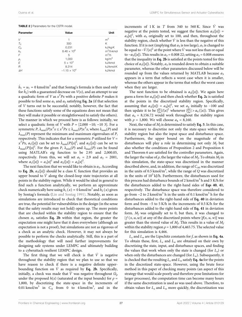
h1 � u1 � 0 kmol/m3 and that Sontag’s formula is then used onlyfor h2) with a guaranteed decrease on V(x), and an attempt to usea quadratic form of V as xTPx with a positive definite P makes itpossible to find some α1 and α2 satisfying Eq. 2a (if that selectionof V turns out to be successful; notably, however, the fact thatthese functions satisfy some of the equations does not mean thatthey will make it possible or straightforward to satisfy the others).The manner in which we proceed here is as follows: initially, weselect a quadratic form of V with P = [2,000 −10; −10 3]. For asymmetric P, λmin(P)x

Tx ≤ xTPx ≤ λmax(P)xTx, where λmin(P) and

λmax(P) represent the minimum and maximum eigenvalues of P,respectively. This indicates that for a symmetric P utilized for V =xTPx, α1(|x|) can be set to λmin(P)|x|

2, and α2(|x|) can be set toλmax(P)|x|

2. For the given P, λmin(P) and λmax(P) can be foundusing MATLAB’s eig function to be 2.95 and 2,000.05,respectively. From this, we will set a1 = 2.9 and a2 = 2001,where α1(|x|) = a1|x|

2 and α2(|x|) = a2|x|2.

The next function that we would like to obtain is α3. Accordingto Eq. 2b, α3(|x|) should be a class K function that provides anupper bound to _V along the closed-loop state trajectories at allpoints in the stability region. While it would be ideal in general tofind such a function analytically, we perform an approximatecheck numerically here using h1(x) � 0 kmol/m3 and h2(x) givenby Sontag’s formula (Lin and Sontag 1991). Notably, as soon assimulations are introduced to check that theoretical conditionsare true, the potential for vulnerabilities in the design (in the sensethat the safety results may not hold) opens up. The more pointsthat are checked within the stability region to ensure that thechosen α3 satisfies Eq. 2b within that region, the greater theexpectation one might have that it does everywhere (although anexpectation is not a proof), but simulations are not as rigorous ofa check as an analytic check. However, it may not always bepossible to perform the checks analytically. Still, this is a part ofthe methodology that will need further improvements fordesigning safe systems under LEMPC and ultimately buildingto a cyberattack-resilient LEMPC design.

The first thing that we will check is that _V is negativethroughout the stability region that we plan to use so that wehave reason to check if there is a negative definite upper-bounding function on _V as required by Eq. 2b. Specifically,initially, a check was made that _V was negative throughout Ωρ

under the proposed h(x) (saturated at the input bounds) for ρ =1,800, by discretizing the state-space in the increments of0.01 kmol/m3 in CA from 0 to 4 kmol/m3, and in the

increments of 1 K in T from 340 to 560 K. Since _V wasnegative at the points tested, we suggest the function α3(|x|) =a3|x|

2, with a3 originally set to 100, and then, throughout thestability region, check whether _V is less than the negative of thisfunction. If it is not (implying that a3 is too large), a3 is changed tobe equal to − _V/|x|2 at the point where _Vwas not less than or equalto −α3(|x|). This results in a3 = 0.008 22; setting a3 = 0.008 ensuresthat the inequality in Eq. 2b is satisfied at the points tested for thischoice of α3(|x|). Notably, a3 is rounded down to obtain a suitableparameter, whereas the other parameters discussed below will berounded up from the values returned by MATLAB because a3appears in a term that reflects a worst case when it is smaller,whereas the others appear in the terms that reflect the worst caseswhen they are larger.

The next function to be obtained is α4(|x|). We again hereguess a form for α4(|x|) and then check whether Eq. 2c is satisfiedat the points in the discretized stability region. Specifically,assuming that α4(|x|) = a4|x|

2, we set a4 initially to −100 andthen update it to be |zVzx|/|x|2 whenever |zVzx|> α4(|x|). This givesthat a4 = 8,156.72 would work throughout the stability regionwith ρ = 1,800. We will choose a4 = 8,160.

Next, the value ofMf is determined to satisfy Eq. 5. In this case,it is necessary to discretize not only the state-space within thestability region but also the input space and disturbance space.Furthermore, the upper bound on the magnitude of thedisturbances will play a role in determining not only Mf butalso whether the conditions of Proposition 2 and Proposition 6and Theorem 6 are satisfied for the controller parameters. Again,the larger the value of ρ, the larger the value ofMf. To obtainMf inthis simulation, the state-space was discretized in the mannerdescribed above, and, in addition, the range of CA0 was discretizedin the units of 0.5 kmol/m3, while the range of Q was discretizedin the units of 105 kJ/h. Furthermore, the disturbances used forthis process had disturbance bounds of 2 kmol/m3 h and 5 K/h forthe disturbances added to the right-hand sides of Eqs 40, 41,respectively. The disturbance space was therefore considered togo from −2 to 2 kmol/m3 h in the units of 0.1 kmol/m3 h for thedisturbances added to the right-hand side of Eq. 40 in deviationform and from −5 to 5 K/h in the increments of 0.5 K/h for thedisturbances added to the right-hand side of Eq. 41 in deviationform. Mf was originally set to 0, but then, it was changed to|f(x, u, w)| at any of the discretized points where |f(x, u, w)| wasgreater than the stored value of Mf. This results in a value of Mf

within the stability region ρ = 1,800 of 4,465.75. The selected valuefor this simulation is 4,466.

Lx and Lw are the Lipschitz constants for f, as shown in Eq. 4a.To obtain these, first, Lx and Lw are obtained on their own bydiscretizing the state, input, and disturbance spaces, and findingthe values that work when only the state is changed (for Lx) orwhen only the disturbances are changed (for Lw). Subsequently, itis checked that the resulting Lx and Lw satisfy Eq. 4a for the pointsin the discretized state-space. However, using the brute forcemethod in this paper of checking many points (an aspect of thisstrategy that would scale poorly and therefore pose limitations forlarger processes), the computation time can become many hoursif the same discretization is used as was used above. Therefore, toobtain values for Lx and Lw more quickly, the discretization was

TABLE 2 | Parameters for the CSTR model.

Parameter Value Unit

V 1 m3

T0 300 KCp 0.231 kJ/kg·Kk0 8.46 × 106 m3/h·kmolF 5 m3/hρL 1,000 kg/m3

E 5 × 104 kJ/kmolR 8.314 kJ/kmol·KΔH −1.15 × 104 kJ/kmol




www.frontiersin.org


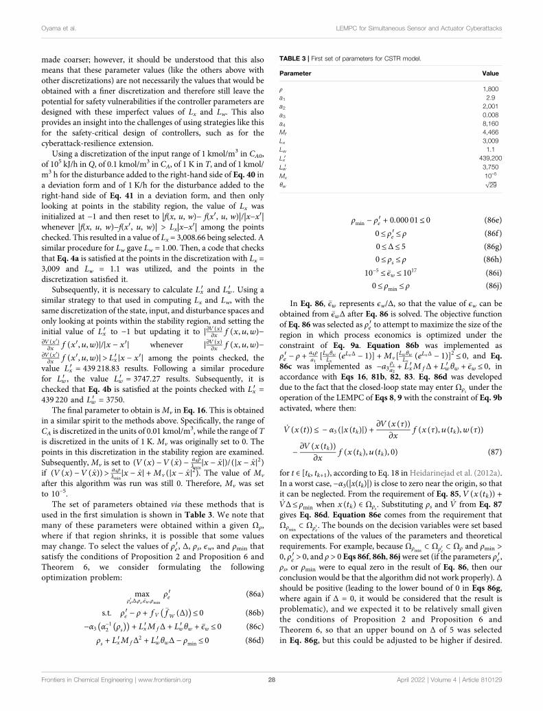
made coarser; however, it should be understood that this alsomeans that these parameter values (like the others above withother discretizations) are not necessarily the values that would beobtained with a finer discretization and therefore still leave thepotential for safety vulnerabilities if the controller parameters aredesigned with these imperfect values of Lx and Lw. This alsoprovides an insight into the challenges of using strategies like thisfor the safety-critical design of controllers, such as for thecyberattack-resilience extension.

Using a discretization of the input range of 1 kmol/m3 in CA0,of 105 kJ/h in Q, of 0.1 kmol/m3 in CA, of 1 K in T, and of 1 kmol/m3 h for the disturbance added to the right-hand side of Eq. 40 ina deviation form and of 1 K/h for the disturbance added to theright-hand side of Eq. 41 in a deviation form, and then onlylooking at points in the stability region, the value of Lx wasinitialized at −1 and then reset to |f(x, u, w)− f(x′, u, w)|/|x−x′|whenever |f(x, u, w)−f(x′, u, w)| > Lx|x−x′| among the pointschecked. This resulted in a value of Lx = 3,008.66 being selected. Asimilar procedure for Lw gave Lw = 1.00. Then, a code that checksthat Eq. 4a is satisfied at the points in the discretization with Lx =3,009 and Lw = 1.1 was utilized, and the points in thediscretization satisfied it.

Subsequently, it is necessary to calculate Lx′ and Lw′ . Using asimilar strategy to that used in computing Lx and Lw, with thesame discretization of the state, input, and disturbance spaces andonly looking at points within the stability region, and setting theinitial value of Lx′ to −1 but updating it to |zV(x)zx f(x, u, w)−zV(x′)zx f(x′, u, w)|/|x − x′| whenever |zV(x)zx f(x, u, w)−

zV(x′)zx f(x′, u, w)|> Lx′ |x − x′| among the points checked, the

value Lx′ � 439 218.83 results. Following a similar procedurefor Lw′ , the value Lw′ � 3747.27 results. Subsequently, it ischecked that Eq. 4b is satisfied at the points checked with Lx′ �439 220 and Lw′ � 3750.

The final parameter to obtain isMv in Eq. 16. This is obtainedin a similar spirit to the methods above. Specifically, the range ofCA is discretized in the units of 0.01 kmol/m3, while the range of Tis discretized in the units of 1 K. Mv was originally set to 0. Thepoints in this discretization in the stability region are examined.Subsequently, Mv is set to (V(x) − V(x) − a4ρ

λmin|x − x|)/(|x − x|2)

if (V(x) − V(x))> a4ρλmin

|x − x| +Mv(|x − x|2). The value of Mv

after this algorithm was run was still 0. Therefore, Mv was setto 10–5.

The set of parameters obtained via these methods that isused in the first simulation is shown in Table 3. We note thatmany of these parameters were obtained within a given Ωρ,where if that region shrinks, it is possible that some valuesmay change. To select the values of ρe′, Δ, ρs, ϵw, and ρmin thatsatisfy the conditions of Proposition 2 and Proposition 6 andTheorem 6, we consider formulating the followingoptimization problem:

maxρe′,Δ,ρs ,�ϵw,ρmin

ρe′ (86a)s.t. ρe′ − ρ + fV

�fW Δ( )( )≤ 0 (86b)−α3 α−1

2 ρs( )( ) + Lx′MfΔ + Lw′ θw + �ϵw ≤ 0 (86c)ρs + Lx′MfΔ2 + Lw′ θwΔ − ρmin ≤ 0 (86d)

ρmin − ρe′ + 0.000 01≤ 0 (86e)0≤ ρe′≤ ρ (86f )0≤Δ≤ 5 (86g)0≤ ρs ≤ ρ (86h)

10−5 ≤ �ϵw ≤ 1017 (86i)0≤ ρmin ≤ ρ (86j)

In Eq. 86, �ϵw represents ϵw/Δ, so that the value of ϵw can beobtained from �ϵwΔ after Eq. 86 is solved. The objective functionof Eq. 86 was selected as ρe′ to attempt to maximize the size of theregion in which process economics is optimized under theconstraint of Eq. 9a. Equation 86b was implemented asρe′ − ρ + a4ρ

a1[LwθwLx

(eLxΔ − 1)] +Mv[LwθwLx(eLxΔ − 1)]2 ≤ 0, and Eq.

86c was implemented as −a3ρsa2 + Lx′MfΔ + Lw′ θw + �ϵw ≤ 0, inaccordance with Eqs 16, 81b, 82, 83. Eq. 86d was developeddue to the fact that the closed-loop state may enter Ωρs under theoperation of the LEMPC of Eqs 8, 9 with the constraint of Eq. 9bactivated, where then:

_V x t( )( )≤ − α3 |x tk( )|( ) + zV x τ( )( )zx

f x τ( ), u tk( ), w τ( )( )

− zV x tk( )( )zx

f x tk( ), u tk( ), 0( ) (87)

for t ∈ [tk, tk+1), according to Eq. 18 in Heidarinejad et al. (2012a).In a worst case, −α3(|x(tk)|) is close to zero near the origin, so thatit can be neglected. From the requirement of Eq. 85, V(x(tk)) +_VΔ≤ ρmin when x(tk) ∈ Ωρs. Substituting ρs and _V from Eq. 87gives Eq. 86d. Equation 86e comes from the requirement thatΩρmin

⊂ Ωρe′ . The bounds on the decision variables were set basedon expectations of the values of the parameters and theoreticalrequirements. For example, because Ωρmin

⊂ Ωρe′ ⊂ Ωρ and ρmin >0, ρe′ > 0, and ρ > 0 Eqs 86f, 86h, 86jwere set (if the parameters ρe′,ρs, or ρmin were to equal zero in the result of Eq. 86, then ourconclusion would be that the algorithm did not work properly). Δshould be positive (leading to the lower bound of 0 in Eqs 86g,where again if Δ = 0, it would be considered that the result isproblematic), and we expected it to be relatively small giventhe conditions of Proposition 2 and Proposition 6 andTheorem 6, so that an upper bound on Δ of 5 was selectedin Eq. 86g, but this could be adjusted to be higher if desired.

TABLE 3 | First set of parameters for CSTR model.

Parameter Value

ρ 1,800a1 2.9a2 2,001a3 0.008a4 8,160Mf 4,466Lx 3,009Lw 1.1Lx′ 439,200Lw′ 3,750Mv 10–5

θw��29

√




www.frontiersin.org


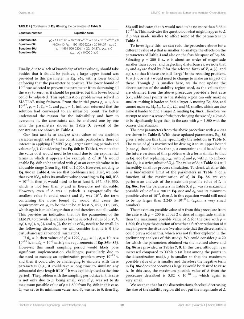
Finally, due to a lack of knowledge of what value �ϵw should takebesides that it should be positive, a large upper bound wasprovided to this parameter in Eq. 86i, with a lower boundenforcing that the parameter be positive. The lower bound of10–5 was selected to prevent the parameter from decreasing allthe way to zero, as it should be positive, but this lower boundcould be adjusted. This optimization problem was solved inMATLAB using fmincon. From the initial guess ρe′ � 1, Δ =10–12, ρs = 1, �ϵw � 1, and ρmin = 1, fmincon returned that thesolution had converged to an infeasible point. To betterunderstand the reason for the infeasibility and how toovercome it, the constraints can be analyzed one by onewith the parameters shown in Table 3. Several of theconstraints are shown in Table 4.

Our first task is to analyze what values of the decisionvariables might satisfy these constraints, particularly those ofinterest in applying LEMPC (e.g., larger sampling periods andvalues of ρe′). Considering first Eq. 86b in Table 4, we note thatthe value of Δ would need to be small due to the exponentialterms in which Δ appears (for example, Δ of 10–5 h wouldenable Eq. 86b to be satisfied with ρe′ at an example value in itsallowable range (from Eq. 86f) of 1,000). However, moving toEq. 86c in Table 4, we see that problems arise. First, we notethat even if �ϵw takes its smallest value according to Eq. 86i, if Δ= 10–5 h, then ρs would need to be at least 9, 957, 459, 550,which is not less than ρ and is therefore not allowable.However, even if Δ was 0 (which is asymptotically thesmallest value it could reach) and �ϵw was 10–5, the termcontaining the noise bound θw would still cause therequirement on ρs to be that it be at least 5, 051, 116, 305,which again is much larger than ρ and therefore not allowable.This provides an indication that for the parameters of theLEMPC to provide guarantees for the selected values of ρ, V, h,α1(·), α2(·), α3(·), and α4(·), the value of θw needs to be small. Inthe following discussion, we will consider that it is 0 (nodisturbances/plant-model mismatch).

If θw = 0, then values of ρe′ � 1799, ρmin = 11, ρs = 10, Δ =10–15 h, and �ϵw � 10−5 satisfy the requirements of Eqs 86b–86j.However, this small sampling period would likely posesignificant implementation challenges, particularly due tothe need to execute an optimization problem every 10–15 h,and then it could also be challenging to simulate with theseparameters (e.g., it could take a long time to simulate anysubstantial time length if 10–15 h was explicitly used as the timeperiod). The problem with the sampling period size in this caseis not only due to ρs being small; even if ρs was set to itsmaximum possible value of ρ = 1,800 from Eq. 86h in this case,�ϵw was set to its minimum value, and θw was set to 0, then Eq.

86c still indicates that Δ would need to be no more than 3.66 ×10–12 h. This motivates the question of what might happen to Δif ρ was made smaller to affect some of the parameters inTable 3.

To investigate this, we can redo the procedure above for adifferent value of ρ that is smaller, to analyze the effects on theparameters of Table 3 and also on the feasible space of Eq. 86.Selecting ρ = 200 (i.e., ρ is about an order of magnitudesmaller than above) and neglecting disturbances, we note thata1 and a2 are fixed by P for the selected form of V, α1(·), andα2(·), so that if these are still “large” in the resulting problem,V, α1(·), or α2(·) would need to change to make an impact onthese. Though ρ is smaller here, we do not update thediscretization of the stability region used, as the values thatare obtained from the above procedure provide a best case(i.e., additional points in the stability region can only make a3smaller, making it harder to find a larger Δ meeting Eq. 86c, andcannot make a4,Mf, Lx, Lw, Lx′ , Lw′ , andMv smaller, which can alsomake it harder to find a larger Δ meeting Eq. 86c). Therefore, weattempt to obtain a sense of whether changing the size of ρ allows Δto be significantly larger than in the case with ρ = 1,800 with thecoarser discretization.

The new parameters from the above procedure with ρ = 200are shown in Table 5. With these updated parameters, Eq. 86gives a solution this time, specifically the solution in Table 6.The value of ρe′ is maximized by driving it to its upper bound(since ρe′ should be less than ρ, a constraint could be added inthe future versions of this problem with a form similar to thatin Eq. 86e but replacing ρmin with ρe′ and ρe with ρ, to enforcethatΩρe′ is a strict subset ofΩρ). The value of Δ in Table 6 is stillincredibly small for process simulation. To check whether thisis a fundamental limit of the parameters in Table 5 or afunction of the maximization of ρe′ in Eq. 86, we canperform an analysis of the maximum possible value of Δ inEq. 86c. For the parameters in Table 5, if ρs was its maximumpossible value of ρ = 200 in Eq. 86c and �ϵw was its minimumpossible value of 10–5, then Δ in this equation would still needto be no larger than 2.245 × 10–10 h (again, a very smallnumber).

The maximum possible value of Δ from this procedure fromthe case with ρ = 200 is about 2 orders of magnitude smallerthan the maximum possible value of Δ for the case with ρ =1,800; this begs the question of whether a further reduction of ρmay improve the situation (we also note that the discretizationcould play a role in this, which was not further explored in thepreliminary analyses of this study). We could consider ρ = 20for which the parameters obtained via the method above andEq. 86 are provided in Tables 7, 8. In this case, although a3 isincreased compared to Table 5 (at least among the points inthe discretization used), ρ is smaller so that the maximumpossible value of ρs is smaller and therefore the negative termin Eq. 86c does not become as large as would be desired to raiseΔ. In this case, the maximum possible value of Δ from theprocedure described is 3.82 × 10–10 h, which again isvery small.

We see then that for the discretizations checked, decreasingthe size of the stability region did not put the magnitude of Δ

TABLE 4 | Constraints of Eq. 86 using the parameters of Table 3.

Equation number Equation form

Equation 86b ρe′ − 11 770.90 + 9970.90e3009Δ + 3.88 × 10−11e6018Δ ≤0Equation 86c −4.00 × 10−6ρs + 1961 556 520Δ + 20194.37 + �ϵw ≤0Equation 86d ρs + 1961 556 520Δ2 + 20,194.37Δ−ρmin ≤ 0Equation 86e ρmin − ρe′ + 0.000 01≤0




www.frontiersin.org


in a reasonable range for the selected for h, V, and αi, i = 1, 2, 3,4. This gives a greater insight into Remark 12, which indicatedthat it is necessary to select h and V such that reasonableparameters can be obtained. Future work could explore otherfunctions h, V, and αi, i = 1, 2, 3, 4 for this process to seewhether there exists any that could result in more reasonablevalues of Δ or not. The results of this section also shed light onwhat changes could aid in making Δ larger (for example, it isseen above that a major reason why Δ is so small in eachsimulation is because a3 is small compared to a2 in each caseand ρs is limited in magnitude by ρ, causing the only negativeterm in Eq. 86c to be small, and then since the terms thatmultiply Δ are large for the given shape of Ωρ, Δmust be smallin each case to prevent the positive term containing Δ fromoverwhelming the negative term containing ρs and preventing�ϵw from being positive as required by Eq. 86i). Although theseresults have not focused directly on the cybersecurity ofcontrol systems, they give some indication of the challengesthat would be faced in working toward developing the controlparameters of a cyberattack-resilient LEMPC meeting thetheory in this work. They indicate that meeting the theoryrequires better strategies than that used in this section forpreventing vulnerabilities.

10 CONCLUSION

This work extended the control/detection strategies developed inOyama and Durand (2020) to handle actuator attacks and caseswhere actuator and sensor attacks can occur simultaneously. Forthe event where multiple attacks are considered, several

integrated control/detection frameworks that pair thedetection strategies designed for single attack-type events wereinvestigated. It was demonstrated that certain combinations ofthe detection strategies can be ineffective to flag both types ofcyberattacks evaluated in this work, while others create acyberattack-resilient structure that enables the detection ofindividual or simultaneous sensor and actuator attack typeswhile ensuring safe operation even if undetected attacksoccur. In particular, the pairing of Detection Strategies 1-Aand 3-S and the pairing of Detection Strategies 2-A and 3-Swere shown to be resilient against both types of cyberattacks. Themajor benefits of these methods are that multiple attackscenarios can be discovered, which adds a layer of protection,and closed-loop stability is guaranteed if an attack policy is notflagged by these two-piece structures. Finally, to characterize thefundamental nature of sensor and actuator attacks, wemathematically defined the concept of cyberattackdiscoverability in the context of process control and stealthyattack policies, which may provide insights for future detectionstrategy development. The potential practical challenges withdesigning LEMPCs meeting theoretical conditions, a precursorstudy for getting the parameters of cyberattack-resilientLEMPCs, elucidated some of the potential challenges withobtaining the parameters meeting the theory that could beaddressed in future work.

DATA AVAILABILITY STATEMENT

The raw data supporting the conclusion of this article will bemade available by the authors, without undue reservation. The

TABLE 5 | Second set of parameters for CSTR model.

Parameter Value

ρ 200a1 2.9a2 2,001a3 1.14a4 8,160Mf 2,660Lx 1,554Lw 0Lx′ 190,800Lw′ 0Mv 10–5

θw 0

TABLE 6 | Equation 86 parameters from the second set of parameters for CSTRmodel in Table 5.

Parameter Value

ρe′ 200.00Δ 1.40 × 10–11

ρs 37.49�ϵw 0.0071ρmin 45.092

TABLE 7 | Third set of parameters for CSTR model.

Parameter Value

ρ 20a1 2.9a2 2,001a3 11.15a4 5,601Mf 2,294Lx 1,221Lw 0Lx′ 126,910Lw′ 0Mv 10–5

θw 0

TABLE 8 | Equation 86 parameters from the third set of parameters for CSTRmodel in Table 7.

Parameter Value

ρe′ 20.00Δ 7.09 × 10–11

ρs 11.11�ϵw 0.021ρmin 13.93




www.frontiersin.org


codes generated for this study will be uploaded to: https://durand.eng.wayne.edu/PublicationResources/index.html.

AUTHOR CONTRIBUTIONS

HO worked on writing the manuscript and developing conceptsand simulations for the manuscript. DM aided in developingsimulations used for obtaining the results in the work and inwriting portions of the work. KR aided in development of theactuator cyberattack-handling procedure. HD supervised thework and aided in writing and editing the manuscript andsimulations and conceptualizing the methodology.

FUNDING

Financial support from the Air Force Office of Scientific Research(award number FA9550-19-1-0059), National ScienceFoundation CNS-1932026 and CBET-1839675, and WayneState University is gratefully acknowledged.

ACKNOWLEDGMENTS

We would like to thank the reviewers, who provided tremendoushelp and insights in their comments that aided us greatly indeveloping the final version of this manuscript.

REFERENCES

Ahrens, J. H., and Khalil, H. K. (2009). High-gain Observers in the Presence ofMeasurement Noise: A Switched-Gain Approach. Automatica 45, 936–943.doi:10.1016/j.automatica.2008.11.012

Ani, U. P. D., He, H., and Tiwari, A. (2017). Review of Cybersecurity Issues inIndustrial Critical Infrastructure: Manufacturing in Perspective. J. CyberSecurity Technol. 1, 32–74. doi:10.1080/23742917.2016.1252211

Bemporad, A., Morari, M., Dua, V., and Pistikopoulos, E. N. (2002). The ExplicitLinear Quadratic Regulator for Constrained Systems. Automatica 38, 3–20.doi:10.1016/s0005-1098(01)00174-1

Brunton, S. L., Proctor, J. L., and Kutz, J. N. (2016). Discovering GoverningEquations from Data by Sparse Identification of Nonlinear DynamicalSystems. Proc. Natl. Acad. Sci. USA 113, 3932–3937. doi:10.1073/pnas.1517384113

Cárdenas, A. A., Amin, S., Lin, Z.-S., Huang, Y.-L., Huang, C.-Y., and Sastry, S.(2011). “Attacks against Process Control Systems: Risk Assessment, Detection,and Response,” in Proceedings of the ACM Asia Conference on Computer &Communications Security, Hong Kong, China.

Chen, S., Wu, Z., and Christofides, P. D. (2020). A Cyber-Secure Control-DetectorArchitecture for Nonlinear Processes. AIChE J. 66, e16907. doi:10.1002/aic.16907

Davis, J., Edgar, T., Graybill, R., Korambath, P., Schott, B., Swink, D., et al. (2015).Smart Manufacturing. Annu. Rev. Chem. Biomol. Eng. 6, 141–160. doi:10.1146/annurev-chembioeng-061114-123255

Ding, D., Han, Q.-L., Ge, X., and Wang, J. (2020). Secure State Estimation andControl of Cyber-Physical Systems: A Survey. IEEE Trans. Syst. Man,Cybernetics: Syst. 51, 176–190.

Durand, H. (2018). A Nonlinear Systems Framework for Cyberattack Preventionfor Chemical Process Control Systems. Mathematics 6, 44. doi:10.3390/math6090169

Durand, H., and Messina, D. (2020). “Enhancing Practical Tractability ofLyapunov-Based Economic Model Predictive Control,” in Proceedings ofthe American Control Conference, Denver, Colorado, 2018–2023. doi:10.23919/acc45564.2020.9147880

Durand, H., and Wegener, M. (2020). Mitigating Safety Concerns and Profit/production Losses for Chemical Process Control Systems underCyberattacks via Design/control Methods. Mathematics 8, 499. doi:10.3390/math8040499

Ellis, M., Durand, H., and Christofides, P. D. (2014a). A Tutorial Review ofEconomic Model Predictive Control Methods. J. Process Control. 24,1156–1178. doi:10.1016/j.jprocont.2014.03.010

Ellis, M., Zhang, J., Liu, J., and Christofides, P. D. (2014b). Robust MovingHorizon Estimation Based Output Feedback Economic Model PredictiveControl. Syst. Control. Lett. 68, 101–109. doi:10.1016/j.sysconle.2014.03.003

Griffith, D. W. (2018). “Advances in Nonlinear Model Predictive Control for Large-Scale Chemical Process Systems,”. Ph.D. thesis (Pittsburgh, Pennsylvania:Carnegie Mellon University).

Heidarinejad, M., Liu, J., and Christofides, P. D. (2012a). Economic ModelPredictive Control of Nonlinear Process Systems Using LyapunovTechniques. AIChE J. 58, 855–870. doi:10.1002/aic.12672

Heidarinejad, M., Liu, J., and Christofides, P. D. (2012b). State-estimation-basedEconomic Model Predictive Control of Nonlinear Systems. Syst. Control. Lett.61, 926–935. doi:10.1016/j.sysconle.2012.06.007

Khalil, H. K. (2002). Nonlinear Systems. Third edn. Upper Saddle River, NewJersey: Prentice-Hall.

Lao, L., Ellis, M., Durand, H., and Christofides, P. D. (2015). Real-timePreventive Sensor Maintenance Using Robust Moving Horizon Estimationand Economic Model Predictive Control. AIChE J. 61, 3374–3389. doi:10.1002/aic.14960

Lin, Y., and Sontag, E. D. (1991). A Universal Formula for Stabilization withBounded Controls. Syst. Control. Lett. 16, 393–397. doi:10.1016/0167-6911(91)90111-q

Mhaskar, P., Liu, J., and Christofides, P. D. (2012). Fault-tolerant Process Control:Methods and Applications. Berlin, Germany: Springer Science & BusinessMedia.

Muñoz de la Peña, D., and Christofides, P. D. (2008). Lyapunov-based ModelPredictive Control of Nonlinear Systems Subject to Data Losses. IEEE Trans.Automat. Contr. 53, 2076–2089. doi:10.1109/tac.2008.929401

Narasimhan, S., El-Farra, N. H., and Ellis, M. J. (2021). Detectability-basedController Design Screening for Processes under MultiplicativeCyberattacks. AIChE J. 68, e17430. doi:10.1002/aic.17430

Oyama, H., and Durand, H. (2020). Integrated Cyberattack Detection and ResilientControl Strategies Using Lyapunov-Based Economic Model Predictive Control.AIChE J. 66, e17084. doi:10.1002/aic.17084

Oyama, H., Rangan, K. K., and Durand, H. (2021). Handling of Stealthy Sensor andActuator Cyberattacks on Evolving Nonlinear Process Systems. J. Adv.Manufacturing Process. 3, e10099. doi:10.1002/amp2.10099

Papachristodoulou, A., and Prajna, S. (2002). “On the Construction of LyapunovFunctions Using the Sum of Squares Decomposition,” in Proceedings of theIEEE Conference on Decision and Control (Las Vegas, Nevada: IEEE), Vol. 3,3482–3487.

Pasqualetti, F., Dörfler, F., and Bullo, F. (2013). Attack Detection and Identificationin Cyber-Physical Systems. IEEE Trans. Automat. Contr. 58, 2715–2729. doi:10.1109/tac.2013.2266831

Qin, S. J., and Badgwell, T. A. (2003). A Survey of Industrial Model PredictiveControl Technology. Control. Eng. Pract. 11, 733–764. doi:10.1016/s0967-0661(02)00186-7

Rangan, K. K., Oyama, H., and Durand, H. (2021). Integrated CyberattackDetection and Handling for Nonlinear Systems with Evolving ProcessDynamics under Lyapunov-Based Economic Model Predictive Control.Chem. Eng. Res. Des. 170, 147–179. doi:10.1016/j.cherd.2021.03.024

Rawlings, J. B., Angeli, D., and Bates, C. N. (2012). “Fundamentals of EconomicModel Predictive Control,” in Proceedings of the IEEE Conference on Decisionand Control, Maui, Hawaii, 3851–3861. doi:10.1109/cdc.2012.6425822

Setola, R., Faramondi, L., Salzano, E., and Cozzani, V. (2019). An Overview ofCyber Attack to Industrial Control System. Chem. Eng. Trans. 77,907–912.



https://durand.eng.wayne.edu/PublicationResources/index.html

https://durand.eng.wayne.edu/PublicationResources/index.html

https://doi.org/10.1016/j.automatica.2008.11.012

https://doi.org/10.1080/23742917.2016.1252211

https://doi.org/10.1016/s0005-1098(01)00174-1

https://doi.org/10.1073/pnas.1517384113

https://doi.org/10.1073/pnas.1517384113

https://doi.org/10.1002/aic.16907


https://doi.org/10.1146/annurev-chembioeng-061114-123255

https://doi.org/10.1146/annurev-chembioeng-061114-123255

https://doi.org/10.3390/math6090169


https://doi.org/10.23919/acc45564.2020.9147880

https://doi.org/10.23919/acc45564.2020.9147880



https://doi.org/10.1016/j.jprocont.2014.03.010

https://doi.org/10.1016/j.sysconle.2014.03.003






https://doi.org/10.1016/0167-6911(91)90111-q

https://doi.org/10.1016/0167-6911(91)90111-q

https://doi.org/10.1109/tac.2008.929401



https://doi.org/10.1002/amp2.10099

https://doi.org/10.1109/tac.2013.2266831

https://doi.org/10.1109/tac.2013.2266831

https://doi.org/10.1016/s0967-0661(02)00186-7

https://doi.org/10.1016/s0967-0661(02)00186-7

https://doi.org/10.1016/j.cherd.2021.03.024

https://doi.org/10.1109/cdc.2012.6425822


www.frontiersin.org


Tuptuk, N., and Hailes, S. (2018). Security of Smart Manufacturing Systems.J. Manufacturing Syst. 47, 93–106. doi:10.1016/j.jmsy.2018.04.007

Wu, Z., Albalawi, F., Zhang, J., Zhang, Z., Durand, H., and Christofides, P. D.(2018). Detecting and Handling Cyber-Attacks in Model PredictiveControl of Chemical Processes. Mathematics 6, 22. doi:10.3390/math6100173

Ye, D., and Luo, S. (2019). A Co-design Methodology for Cyber-Physical Systemsunder Actuator Fault and Cyber Attack. J. Franklin Inst. 356, 1856–1879.doi:10.1016/j.jfranklin.2019.01.009

Conflict of Interest: The authors declare that the research was conducted in theabsence of any commercial or financial relationships that could be construed as apotential conflict of interest.

Publisher’s Note: All claims expressed in this article are solely those of the authorsand do not necessarily represent those of their affiliated organizations, or those ofthe publisher, the editors and the reviewers. Any product that may be evaluated inthis article, or claim that may be made by its manufacturer, is not guaranteed orendorsed by the publisher.

Copyright © 2022 Oyama, Messina, Rangan and Durand. This is an open-accessarticle distributed under the terms of the Creative Commons Attribution License (CCBY). The use, distribution or reproduction in other forums is permitted, provided theoriginal author(s) and the copyright owner(s) are credited and that the originalpublication in this journal is cited, in accordance with accepted academic practice.No use, distribution or reproduction is permitted which does not comply withthese terms.



https://doi.org/10.1016/j.jmsy.2018.04.007



https://doi.org/10.1016/j.jfranklin.2019.01.009

https://creativecommons.org/licenses/by/4.0/

https://creativecommons.org/licenses/by/4.0/


www.frontiersin.org


Lyapunov-Based Economic Model Predictive Control for ...

Documents