THÈSE présentée à L’U NIVERSITÉ B ORDEAUX Ecole doctorale des Sciences Physiques et de l’Ingénieur par Victor Grimblatt P OUR OBTENIR LE GRADE DE D OCTEUR L’U NIVERSITÉ B ORDEAUX S PÉCIALITÉ : ÉLECTRONIQUE ————————— DESIGN OF AN INTEGRATED DIGITAL CIRCUIT FOR THE I NTERNET OF THINGS (I OT) APPLIED TO AGRONOMY ————————— Soutenue le : 22 Octobre 2021 Après avis de : M. Giovanni DE MICHELI Full Professor EPFL Rapporteur Andrei VLADIMIRESCU Full Professor University of California Berkeley Rapporteur Devant la commission d’examen formée de : M. Giovanni DE MICHELI Full Professor EPFL Rapporteur Danilo DEMARCHI Professore Associato Politecnico di Torino Examinateur Yann DEVAL Professeur Bordeaux INP Président Antun DOMIC Former CTO Synopsys Examinateur Guillaume FERRÉ Maitre de Conférences, HDR Bordeaux INP Co-encadrant Christophe J ÉGO Professeur Bordeaux INP Directeur Francois RIVET Maitre de Conférences, HDR Bordeaux INP Co-encadrant Andrei VLADIMIRESCU Full Professor University of California Berkeley Rapporteur

Welcome message from author
This document is posted to help you gain knowledge. Please leave a comment to let me know what you think about it! Share it to your friends and learn new things together.
Transcript
THÈSE
présentée à
L’UNIVERSITÉ BORDEAUXEcole doctorale des Sciences Physiques et de l’Ingénieur
par Victor GrimblattPOUR OBTENIR LE GRADE DE
DOCTEUR
L’UNIVERSITÉ BORDEAUX
SPÉCIALITÉ : ÉLECTRONIQUE
—————————DESIGN OF AN INTEGRATED DIGITAL CIRCUIT FOR THE INTERNET OF THINGS (IOT)
APPLIED TO AGRONOMY
—————————
Soutenue le : 22 Octobre 2021
Après avis de :
M. Giovanni DE MICHELI Full Professor EPFL Rapporteur
Andrei VLADIMIRESCU Full Professor University of California Berkeley Rapporteur
Devant la commission d’examen formée de :
M. Giovanni DE MICHELI Full Professor EPFL Rapporteur
Danilo DEMARCHI Professore Associato Politecnico di Torino Examinateur
Yann DEVAL Professeur Bordeaux INP Président
Antun DOMIC Former CTO Synopsys Examinateur
Guillaume FERRÉ Maitre de Conférences, HDR Bordeaux INP Co-encadrant
Christophe JÉGO Professeur Bordeaux INP Directeur
Francois RIVET Maitre de Conférences, HDR Bordeaux INP Co-encadrant
Andrei VLADIMIRESCU Full Professor University of California Berkeley Rapporteur
2
”Il y a des hommes qui luttent un jour et ils sont bons,
autres luttent un an et ils sont meilleurs,
il y a ceux qui luttent pendant de nombreuses années et ils sont très bons,
mais il y a ceux qui luttent toute leur vie et ceux-là sont les indispensables”
Bertolt Brecht

Remerciements
A Maria Luisa, Nicolas et Apolo,
à ma famille,
à mes amis.
A mes professeurs et encadrants,
au laboratoire IMS.
Contents
List of Abbreviations 15
List of Notations 17
Introduction 19
1 IoT and Smart Agriculture 231.1 Motivations . . . . . . . . . . . . . . . . . . . . . . . . . . . . . . . . . . . . . . . . . 24
1.2 Problem Definition . . . . . . . . . . . . . . . . . . . . . . . . . . . . . . . . . . . . . 28
1.2.1 The Plant - P . . . . . . . . . . . . . . . . . . . . . . . . . . . . . . . . . . . . 29
1.2.2 The Soil - S . . . . . . . . . . . . . . . . . . . . . . . . . . . . . . . . . . . . . 31
1.2.3 The Environment - E . . . . . . . . . . . . . . . . . . . . . . . . . . . . . . . . 38
1.2.4 Summary . . . . . . . . . . . . . . . . . . . . . . . . . . . . . . . . . . . . . . 40
1.3 Technologies for Agriculture . . . . . . . . . . . . . . . . . . . . . . . . . . . . . . . . 41
1.3.1 Internet of Things . . . . . . . . . . . . . . . . . . . . . . . . . . . . . . . . . . 41
1.3.2 Communication technology - LPWAN . . . . . . . . . . . . . . . . . . . . . . . 44
1.3.3 State of the Art . . . . . . . . . . . . . . . . . . . . . . . . . . . . . . . . . . . 46
1.4 My Contributions . . . . . . . . . . . . . . . . . . . . . . . . . . . . . . . . . . . . . . 49
2 How to Measure Important Parameters for Plant Growth and Health 512.1 Parameters Measurement . . . . . . . . . . . . . . . . . . . . . . . . . . . . . . . . . . 52
2.1.1 Measurement of Water . . . . . . . . . . . . . . . . . . . . . . . . . . . . . . . 53
2.1.2 Measurement of Nutrients . . . . . . . . . . . . . . . . . . . . . . . . . . . . . 55
2.1.3 Soil pH Measurement . . . . . . . . . . . . . . . . . . . . . . . . . . . . . . . 58
2.1.4 Soil Temperature Measurement . . . . . . . . . . . . . . . . . . . . . . . . . . 61
2.1.5 Soil Salinity Measurement . . . . . . . . . . . . . . . . . . . . . . . . . . . . . 62
2.1.6 The Light . . . . . . . . . . . . . . . . . . . . . . . . . . . . . . . . . . . . . . 63
2.1.7 The Weather . . . . . . . . . . . . . . . . . . . . . . . . . . . . . . . . . . . . 63
2.1.8 Summary . . . . . . . . . . . . . . . . . . . . . . . . . . . . . . . . . . . . . . 63
5
6 Contents
2.2 Experimental Laboratory at Home . . . . . . . . . . . . . . . . . . . . . . . . . . . . . 64
2.2.1 Experiment 1: Chives - Spring . . . . . . . . . . . . . . . . . . . . . . . . . . . 64
2.2.2 Experiment 2 - Cherry tomatoes - Summer . . . . . . . . . . . . . . . . . . . . 68
2.2.3 Experiment 3 - Cherry tomatoes - Summer . . . . . . . . . . . . . . . . . . . . 72
2.2.4 Experiment 4 - Bell Pepper - End of Fall . . . . . . . . . . . . . . . . . . . . . 74
2.3 Parameters Measurement and their Interrelation . . . . . . . . . . . . . . . . . . . . . . 76
3 A Dedicated SoC for Smart Agriculture 793.1 The IoT System and the SoC . . . . . . . . . . . . . . . . . . . . . . . . . . . . . . . . 80
3.1.1 Main Architecture of the System . . . . . . . . . . . . . . . . . . . . . . . . . . 82
3.1.2 Proof of Concept . . . . . . . . . . . . . . . . . . . . . . . . . . . . . . . . . . 84
3.1.3 SoC Architecture . . . . . . . . . . . . . . . . . . . . . . . . . . . . . . . . . . 86
3.2 SoC Design Flow . . . . . . . . . . . . . . . . . . . . . . . . . . . . . . . . . . . . . . 90
3.2.1 Register Transfer Level (RTL) Generation . . . . . . . . . . . . . . . . . . . . . 91
3.2.2 FPGA Implementation Option . . . . . . . . . . . . . . . . . . . . . . . . . . . 92
3.2.3 ASIC Implementation Option . . . . . . . . . . . . . . . . . . . . . . . . . . . 93
3.3 IP Usage . . . . . . . . . . . . . . . . . . . . . . . . . . . . . . . . . . . . . . . . . . . 97
3.3.1 The processor . . . . . . . . . . . . . . . . . . . . . . . . . . . . . . . . . . . . 97
3.3.2 Memories . . . . . . . . . . . . . . . . . . . . . . . . . . . . . . . . . . . . . . 97
3.3.3 I/O Peripherals . . . . . . . . . . . . . . . . . . . . . . . . . . . . . . . . . . . 97
3.4 SoC and System Power Analysis . . . . . . . . . . . . . . . . . . . . . . . . . . . . . . 98
3.5 Connecting the SoC to the Outside World . . . . . . . . . . . . . . . . . . . . . . . . . 99
4 The AgriFood Community 1034.1 The Community I have Found and Where It is Now . . . . . . . . . . . . . . . . . . . . 104
4.1.1 Seasonal School . . . . . . . . . . . . . . . . . . . . . . . . . . . . . . . . . . 104
4.1.2 FoodCAS Community . . . . . . . . . . . . . . . . . . . . . . . . . . . . . . . 107
4.2 How Technology Can Help to Feed the Humanity . . . . . . . . . . . . . . . . . . . . . 108
4.3 My Contribution to the AgriFood Community . . . . . . . . . . . . . . . . . . . . . . . 111
4.4 Next Steps and Future Research . . . . . . . . . . . . . . . . . . . . . . . . . . . . . . 114
4.4.1 Lack of Low-Power and Low-Cost Sensors . . . . . . . . . . . . . . . . . . . . 115
4.4.2 Equation, model and interrelation of plant’s parameters . . . . . . . . . . . . . . 115
4.4.3 Better understanding of plants growth for better IoT systems . . . . . . . . . . . 118
4.4.4 Enhance capabilities of the SoC . . . . . . . . . . . . . . . . . . . . . . . . . . 121
4.5 Conclusion . . . . . . . . . . . . . . . . . . . . . . . . . . . . . . . . . . . . . . . . . 121
Conclusion 123
6
Contents 7
Publications 125
Bibliography 127
A Appendix A 135A.1 Nutrients . . . . . . . . . . . . . . . . . . . . . . . . . . . . . . . . . . . . . . . . . . 136
A.1.1 Macronutrients . . . . . . . . . . . . . . . . . . . . . . . . . . . . . . . . . . . 136
A.1.2 Micronutrients . . . . . . . . . . . . . . . . . . . . . . . . . . . . . . . . . . . 137
A.2 Soil Temperature . . . . . . . . . . . . . . . . . . . . . . . . . . . . . . . . . . . . . . 139
A.2.1 Amount of Heat Supplied at the Surface . . . . . . . . . . . . . . . . . . . . . . 139
A.2.2 Amount of Heat Dissipated from the Surface . . . . . . . . . . . . . . . . . . . 139
A.2.3 Soil Temperature Effects . . . . . . . . . . . . . . . . . . . . . . . . . . . . . . 139
A.3 Light . . . . . . . . . . . . . . . . . . . . . . . . . . . . . . . . . . . . . . . . . . . . . 140
A.3.1 Light Quantity . . . . . . . . . . . . . . . . . . . . . . . . . . . . . . . . . . . 140
A.3.2 Light Quality . . . . . . . . . . . . . . . . . . . . . . . . . . . . . . . . . . . . 141
A.3.3 Light Duration . . . . . . . . . . . . . . . . . . . . . . . . . . . . . . . . . . . 142
B Appendix B 143B.1 Floorplan . . . . . . . . . . . . . . . . . . . . . . . . . . . . . . . . . . . . . . . . . . 144
B.2 SoC Gate Count . . . . . . . . . . . . . . . . . . . . . . . . . . . . . . . . . . . . . . . 145
B.3 RAM Bits Allocation . . . . . . . . . . . . . . . . . . . . . . . . . . . . . . . . . . . . 147
B.4 Core Registers . . . . . . . . . . . . . . . . . . . . . . . . . . . . . . . . . . . . . . . . 147
B.5 Instructions . . . . . . . . . . . . . . . . . . . . . . . . . . . . . . . . . . . . . . . . . 149
B.6 Interrupts . . . . . . . . . . . . . . . . . . . . . . . . . . . . . . . . . . . . . . . . . . 153
B.7 PADs . . . . . . . . . . . . . . . . . . . . . . . . . . . . . . . . . . . . . . . . . . . . 155
Abstract 161
7

8 Contents
8
List of Figures
1.1 Planetary Boundaries [1] . . . . . . . . . . . . . . . . . . . . . . . . . . . . . . . . . . 25
1.2 Doughnut Economy [2] . . . . . . . . . . . . . . . . . . . . . . . . . . . . . . . . . . . 27
1.3 Arable Land in Hectares/Person [3] . . . . . . . . . . . . . . . . . . . . . . . . . . . . 27
1.4 Farm size distribution [4] . . . . . . . . . . . . . . . . . . . . . . . . . . . . . . . . . . 29
1.5 Global Land Use for Food Production [5] . . . . . . . . . . . . . . . . . . . . . . . . . 30
1.6 Observation of nutrient deficiency on leaves . . . . . . . . . . . . . . . . . . . . . . . . 31
1.7 Soil Texture Pyramid [6] . . . . . . . . . . . . . . . . . . . . . . . . . . . . . . . . . . 32
1.8 Capillaries Forces . . . . . . . . . . . . . . . . . . . . . . . . . . . . . . . . . . . . . . 33
1.9 Soil Moisture Content . . . . . . . . . . . . . . . . . . . . . . . . . . . . . . . . . . . . 34
1.10 The effect of soil pH on nutrient availability [7] . . . . . . . . . . . . . . . . . . . . . . 37
1.11 IoT Disambiguation [8] . . . . . . . . . . . . . . . . . . . . . . . . . . . . . . . . . . . 41
1.12 IoT Architecture [9] . . . . . . . . . . . . . . . . . . . . . . . . . . . . . . . . . . . . . 43
2.1 Sensor types based on their operating principles [10] . . . . . . . . . . . . . . . . . . . 56
2.2 Colorimeter system [11] . . . . . . . . . . . . . . . . . . . . . . . . . . . . . . . . . . 57
2.3 Relation NPK and RGB - Wavelengths in nm . . . . . . . . . . . . . . . . . . . . . . . 57
2.4 A prototype sensor NPK . . . . . . . . . . . . . . . . . . . . . . . . . . . . . . . . . . 58
2.5 The Atlas Scientific pH Probe [12] . . . . . . . . . . . . . . . . . . . . . . . . . . . . . 60
2.6 Classification of temperature sensors [13] . . . . . . . . . . . . . . . . . . . . . . . . . 61
2.7 DS18B20 - Simplified block diagram [14] . . . . . . . . . . . . . . . . . . . . . . . . . 62
2.8 Experiment 1 - Chives / Spring . . . . . . . . . . . . . . . . . . . . . . . . . . . . . . . 65
2.9 Soil temperature and soil moisture over time . . . . . . . . . . . . . . . . . . . . . . . . 66
2.10 Soil temperature over soil moisture . . . . . . . . . . . . . . . . . . . . . . . . . . . . . 67
2.11 Experiment 2 - Cherry Tomatoes / Summer . . . . . . . . . . . . . . . . . . . . . . . . 69
2.12 Experiment 2 - Cherry Tomatoes / Summer . . . . . . . . . . . . . . . . . . . . . . . . 70
2.13 Soil moisture resistive and capacitive sensors over time . . . . . . . . . . . . . . . . . . 71
2.14 Soil temperature and environment temperature over time . . . . . . . . . . . . . . . . . 72
9
10 List of Figures
2.15 Environment temperature over soil moisture . . . . . . . . . . . . . . . . . . . . . . . . 72
2.16 Soil temperature and soil moisture over time for a dry soil . . . . . . . . . . . . . . . . . 73
2.17 Soil temperature and soil moisture over time for a wet soil . . . . . . . . . . . . . . . . 74
2.18 Soil and environment temperature over time - End of Fall . . . . . . . . . . . . . . . . . 75
2.19 Moisture over time - End of Fall . . . . . . . . . . . . . . . . . . . . . . . . . . . . . . 76
3.1 Design Flow for the IoT System . . . . . . . . . . . . . . . . . . . . . . . . . . . . . . 81
3.2 Edge architecture overview . . . . . . . . . . . . . . . . . . . . . . . . . . . . . . . . . 83
3.3 Edge architecture overview . . . . . . . . . . . . . . . . . . . . . . . . . . . . . . . . . 84
3.4 Prototype on DesignWare EM Starter Kit . . . . . . . . . . . . . . . . . . . . . . . . . 85
3.5 Internal view of the prototype . . . . . . . . . . . . . . . . . . . . . . . . . . . . . . . . 85
3.6 External view of the prototype . . . . . . . . . . . . . . . . . . . . . . . . . . . . . . . 85
3.7 SoC main architecture . . . . . . . . . . . . . . . . . . . . . . . . . . . . . . . . . . . . 87
3.8 32 bits processor AHB bus based system . . . . . . . . . . . . . . . . . . . . . . . . . . 89
3.9 SoC architecture . . . . . . . . . . . . . . . . . . . . . . . . . . . . . . . . . . . . . . . 89
3.10 Synopsys recommended SoC design Flow . . . . . . . . . . . . . . . . . . . . . . . . . 90
3.11 ARChitect instantiation window . . . . . . . . . . . . . . . . . . . . . . . . . . . . . . 91
3.12 FPGA implementation options . . . . . . . . . . . . . . . . . . . . . . . . . . . . . . . 93
3.13 SoC top level schematic . . . . . . . . . . . . . . . . . . . . . . . . . . . . . . . . . . . 95
3.14 CPU schematic . . . . . . . . . . . . . . . . . . . . . . . . . . . . . . . . . . . . . . . 95
3.15 Memories schematic . . . . . . . . . . . . . . . . . . . . . . . . . . . . . . . . . . . . 95
3.16 Top level of the SoC including muxes and decoders . . . . . . . . . . . . . . . . . . . . 101
3.17 PAD schematic . . . . . . . . . . . . . . . . . . . . . . . . . . . . . . . . . . . . . . . 101
4.1 IEEE CAS seasonal school flyer . . . . . . . . . . . . . . . . . . . . . . . . . . . . . . 106
4.2 Seasonal school book cover . . . . . . . . . . . . . . . . . . . . . . . . . . . . . . . . . 106
4.3 FoodCAS 2021 Program . . . . . . . . . . . . . . . . . . . . . . . . . . . . . . . . . . 108
4.4 United Nations Sustainable Development Goals [15] . . . . . . . . . . . . . . . . . . . 110
4.5 Regenerative agriculture principles [16] . . . . . . . . . . . . . . . . . . . . . . . . . . 110
4.6 My Lettuces . . . . . . . . . . . . . . . . . . . . . . . . . . . . . . . . . . . . . . . . . 112
4.7 My tomatoes . . . . . . . . . . . . . . . . . . . . . . . . . . . . . . . . . . . . . . . . 113
4.8 Vegetables . . . . . . . . . . . . . . . . . . . . . . . . . . . . . . . . . . . . . . . . . . 116
4.9 Cherries . . . . . . . . . . . . . . . . . . . . . . . . . . . . . . . . . . . . . . . . . . . 117
4.10 Nuts . . . . . . . . . . . . . . . . . . . . . . . . . . . . . . . . . . . . . . . . . . . . . 117
4.11 Greenhouse . . . . . . . . . . . . . . . . . . . . . . . . . . . . . . . . . . . . . . . . . 118
4.12 Lettuce eaten by birds . . . . . . . . . . . . . . . . . . . . . . . . . . . . . . . . . . . . 120
10

List of Figures 11
A.1 Light compensation point and light saturation point . . . . . . . . . . . . . . . . . . . . 141
11

12 List of Figures
12
List of Tables
1.1 Mobility of Nutrients . . . . . . . . . . . . . . . . . . . . . . . . . . . . . . . . . . . . 35
1.2 Plant Response to Humidity [17] . . . . . . . . . . . . . . . . . . . . . . . . . . . . . . 40
1.3 Growth Parameters . . . . . . . . . . . . . . . . . . . . . . . . . . . . . . . . . . . . . 40
2.1 Parameters and Sensors . . . . . . . . . . . . . . . . . . . . . . . . . . . . . . . . . . . 64
2.2 Experiments Summary . . . . . . . . . . . . . . . . . . . . . . . . . . . . . . . . . . . 76
3.1 Architecture features after synthesis . . . . . . . . . . . . . . . . . . . . . . . . . . . . 94
3.2 Architecture features after physical synthesis without pads . . . . . . . . . . . . . . . . 96
3.3 SoC layout without Pads . . . . . . . . . . . . . . . . . . . . . . . . . . . . . . . . . . 96
3.4 Power consumption of the architecture . . . . . . . . . . . . . . . . . . . . . . . . . . . 98
3.5 PAD Truth Table . . . . . . . . . . . . . . . . . . . . . . . . . . . . . . . . . . . . . . 100
4.1 Next Steps . . . . . . . . . . . . . . . . . . . . . . . . . . . . . . . . . . . . . . . . . . 122
B.1 SoC Gate Count . . . . . . . . . . . . . . . . . . . . . . . . . . . . . . . . . . . . . . . 146
B.2 RAM Bits Allocation . . . . . . . . . . . . . . . . . . . . . . . . . . . . . . . . . . . . 147
B.3 SoC core registers . . . . . . . . . . . . . . . . . . . . . . . . . . . . . . . . . . . . . . 148
B.4 SoC’s instructions . . . . . . . . . . . . . . . . . . . . . . . . . . . . . . . . . . . . . 152
B.5 SoC’s interrupts . . . . . . . . . . . . . . . . . . . . . . . . . . . . . . . . . . . . . . 154
B.6 Input PADs distribution . . . . . . . . . . . . . . . . . . . . . . . . . . . . . . . . . . 159
13

14 List of Tables
14
List of Abbreviations
3GPP 3rd Generation Partnership Project
A/D Analog-to-Digital
AAF Anti-Aliasing Filter
ADC Analog-to-Digital Converter
ADMS Automated Decision-Making Systems
AHB Advanced High-performance bus
APB Advanced Peripheral bus
ASIC Application-Specific Integrated Circuit
CAGR Compound Annual Growth Rate
CCT Customer confidence tests
CES Consumer Electronic Show
CMOS Complementary MOS
DAC Digital-to-analog converter
DCCM Data Closely Coupled Memory
DSP Digital Signal Processor
DUT Device Under Test
EC electrical conductivity
ENOB Effective Number of Bits
FAO Food and Agriculture Organization
FC Field Capacity
FoodCAS Circuits and Systems for better quality foods
GHG Greenhouse Gas
GPIO General Purpose Input/Output
GSM Global System for Mobile
HW Hardware
I2C Inter-Integrated Circuit
IC Integrated Circuit
ICCM Instruction Closely Coupled Memory
15
16 List of Tables
ICECS International Conference on Electronics, Circuits, and Systems
IoT Internet of Things
IP Intellectual Property
ISCAS International Symposium on Circuits and Systems
ISFET Ion Sensitive Field Electric Transistor
IT irrigation threshold
Lab@Home Laboratory at Home
Li-Fi Light Fidelity
LoRa Long Range
LPWAN Low-Power Wide Area Network
MIPS Million Instructions Per Second
MOS Metal Oxide Semiconductor
NB-IoT Narrowband-IoT
NPK Nitrogen, Phosphorous, and Potassium
PA Precision Agriculture
PCB Printed Circuit Board
PLS Post Layout Simulation
PPA Performance, Power and Area
PWM Pulse-Width Modulation
PWP Permanent Wilting Point
RDF Reference Design Flow
RF Radio-Frequency
RPMA Random phase multiple access
RTD resistance temperature detector
RTL Register Transfer Level
SDG Sustainable Development Goals
SIG Special Interest Group
SNR Signal-to-Noise ratio
SoC System on Chip
SPI Serial Peripheral Interface
SPICE Simulation Program with Integrated Circuit Emphasis
STA Static Time Analysis
SW Software
TDR Time-Domain Reflectometer
UART Universal Asynchronous Receiver-Transmitter
UN United Nations
UPF Unified Power Format
UV ultraviolet
VHDL Very high-speed integrated circuits Hardware Description Language
VOC Volatile Organic Compound
16
List of Notations
E Environment
ET Environment Temperature
G Growth of the plant
L Light
Nu Nutrients
P Plant
pH potential of Hydrogen
Rh Air Relative Humidity
S Soil
Sa Salinity
ST Soil Temperature
W Water
We Weather
17

18 List of Tables
18
Introduction
World population keeps on growing. There are almost 8 billions people on the planet, and the estimation
is that there is going to be 10 billions by 2050. Based on these numbers, the Food and Agriculture Or-
ganization of the United Nations (FAO) estimates that agricultural production needs to increase by 70%
to be able to feed the whole population in 2050. On the other hand, agriculture is responsible for the
excess on 4 out off the 9 planetary boundaries presented in the Chapter 1, especially the biosphere in-
tegrity and biogeochemical flows. Agriculture is then facing an enormous dilemma: how to increase the
productivity while taking into account the planetary boundaries. Small and medium farmers are looking
for techniques that could help them to increase their productivity, so they can face the feeding issue the
humanity will encounter in the next decades. However, increasing the productivity without a change in
the way they produce will continue to impact the planet boundaries and the global warming as well. It is
important and even mandatory to find a different way to handle food production while keeping the planet
safe.
Smart Agriculture and Agriculture 4.0 have been trying to address this problem through the design
and implementation of electronic systems based on the Automated Decision Making Systems (ADMS)
and the Internet of Things (IoT) concepts. Those systems provide reasonable results in an important
number of cases, however their usage at small and medium farms is very low, which is,by the way, the
majority of farms around the world. It has been found that small and medium farmers are far from tech-
nology mostly because its cost and because technology for the agriculture is difficult to implement and
use. Several solutions available in the market are mounted on tractors or other agricultural machines,
so the power consumed by those solutions is not a real issue as the supply is coming from the machine
they are installed. Small and medium farmers, especially in under developed countries, do not have this
kind of equipment. So, to be able to provide a useful system to small and medium farmers, a system
that can help them to improve their productivity without affecting the planet, a system that is low power,
low cost, and easy is what is needed. All those requirements have to be considered in the design and
implementation of such a system.
Besides that, an important part of the commercial systems for agriculture are based on platforms
19
20 List of Tables
or components out off the shelf that are not always the best choice for the target applications as they
can be too expensive, they can consume too much power, and even they are not adapted to the agricul-
tural environment (outdoor and dirty environment). In addition, those system are not considering all the
parameters influencing plant growth and health. They are not customized by species and they consider
that all soils are identical which is not the case. More details about this consideration are presented in
Chapters 1 and 2.
The main objective of this research work is the study of the parameters affecting plant growth
and health and how to use them on an IoT system dedicated to small and medium farmers. As this IoT
system has to be specific to the agricultural applications, a specific circuit (SoC) is designed taking in
consideration the requirements that have been defined for small and medium farmers.
Chapter 1 introduces the motivations of the research work. Then, a deep analysis of the param-
eters influencing the growth and health of plants is presented. The ones that are selected for the IoT
system being designed as part of this research work are mentioned. An equation modeling the growth of
plants is also sketched as part of this chapter. Technologies applied to the agriculture are studied based
on a detailed state of the art analysis. The chapter also includes information on suitable communication
technologies for the target applications. The chapter ends with an explanation of my contributions to the
technology applied to agriculture and a detailed description of the requirements of the system for small
and medium farmers that is designed as part of this research work.
Chapter 2 presents a detailed analysis on how the parameters affecting the growth and health of
plants and presented in Chapter 1 can be measured and added to an IoT system dedicated to agriculture.
To validate the usage of the presented sensors and the architecture of the system designed, several ex-
periments with crops and sensors are detailed and some preliminary conclusions about the interaction
between parameters are mentioned. These conclusions are considered for the rest of the research work
and for the growth equation presented in Chapter 1.
Chapter 3 details the design of a dedicated SoC for smart agriculture, based on the requirements
presented in the previous chapters (Chapters 1 and 2). It includes the main characteristics of the SoC, the
used design flow, the used IP for its implementation, and the results of the design presenting the power,
performance, and area (PPA) of the SoC. An analysis of the energy required by the system in operation
is also presented and a battery is proposed for the implementation of the system in the field, considering
that the system should be operational for at least three years without human intervention.
20
List of Tables 21
Chapter 4 depicts the AgriFood community I have encountered, which I helped growing during
the past 5 years. I discussed on how technology can help to feed the humanity and I listed my actions
inside the AgriFood community. Finally, I draw the next steps for this research and for the technology
for the AgriFood in general. Several research topics are presented in this Chapter and I hope they will
influence the AgriFood community to work on the directions I’m proposing.
Smart agriculture or Agriculture 4.0 is a passionate topic and a lot of additional things can still
be done as a continuation of this work. I invite the community to read this manuscript thinking of how
we can improve the productivity of the soil without impacting the planet. I hope that several ideas and
projects will come to your mind and together we will be able to feed a growing population and save our
planet.
This document presents the work I have done over almost 4 years during my PhD. This work
have created several scientific publications, keynotes, and workshops that are detailed in the Publication
section of this document (4.5).
21

22 List of Tables
22
CHAPTER
1IOT AND SMART
AGRICULTURE
Sommaire1.1 Motivations . . . . . . . . . . . . . . . . . . . . . . . . . . . . . . . . . . . . . . . . 24
1.2 Problem Definition . . . . . . . . . . . . . . . . . . . . . . . . . . . . . . . . . . . . 28
1.2.1 The Plant - P . . . . . . . . . . . . . . . . . . . . . . . . . . . . . . . . . . . 29
1.2.2 The Soil - S . . . . . . . . . . . . . . . . . . . . . . . . . . . . . . . . . . . . 31
1.2.3 The Environment - E . . . . . . . . . . . . . . . . . . . . . . . . . . . . . . . 38
1.2.4 Summary . . . . . . . . . . . . . . . . . . . . . . . . . . . . . . . . . . . . . 40
1.3 Technologies for Agriculture . . . . . . . . . . . . . . . . . . . . . . . . . . . . . . 41
1.3.1 Internet of Things . . . . . . . . . . . . . . . . . . . . . . . . . . . . . . . . . 41
1.3.2 Communication technology - LPWAN . . . . . . . . . . . . . . . . . . . . . . 44
1.3.3 State of the Art . . . . . . . . . . . . . . . . . . . . . . . . . . . . . . . . . . 46
1.4 My Contributions . . . . . . . . . . . . . . . . . . . . . . . . . . . . . . . . . . . . 49
23
24 Chapter 1. IoT and Smart Agriculture
1.1 Motivations
Few years ago, I was in my countryside house and I realized that it could be good idea to plant some
crops. So, I could get some organic and good food for my own consumption. I started with some
tomatoes and lettuces. Tomatoes grew very well and I was able to eat a good tomato salad that was
fantastic: nice color and great taste. I also did my own tomato sauce, that was also great. Lettuces were
quite different and I faced several issues. Only 10 lettuces out of the 50 I planted grew. I was surprised
as I irrigated my lettuces in the same way I did for my tomatoes and the results were so different. As an
engineer and researcher I started to study how plants grow and I found that irrigation is not enough. I
found that the grow and health of crops depend on a lot of different physical processes and parameters
that can be monitored and even some of them controlled so we can ensure that they are kept at reasonable
values.
During my research I also found that agriculture was one of the biggest responsible for the emission of
the Greenhouse Gas (GHG). According to the Food and Agriculture Organization (FAO) United Nations
(UN) one third of global GHG emissions is caused by agriculture, forestry, and change of land use. At
the same time the agriculture is one of the most climate-sensitive sectors, so climate change is a major
challenge for agriculture. I have also found that agriculture is the heaviest consumer of planet’s available
freshwater using more than 70% of "blue water". Agriculture demand of water is estimated to increase
by 19% by 2050. An important part of this water is wasted as irrigation is not controlled, as I did for my
lettuces.
I also found that population is growing and we will need to produce more food to be able to meet the
"food safety" defined by United Nations. It is complicated to talk about increasing the productivity as
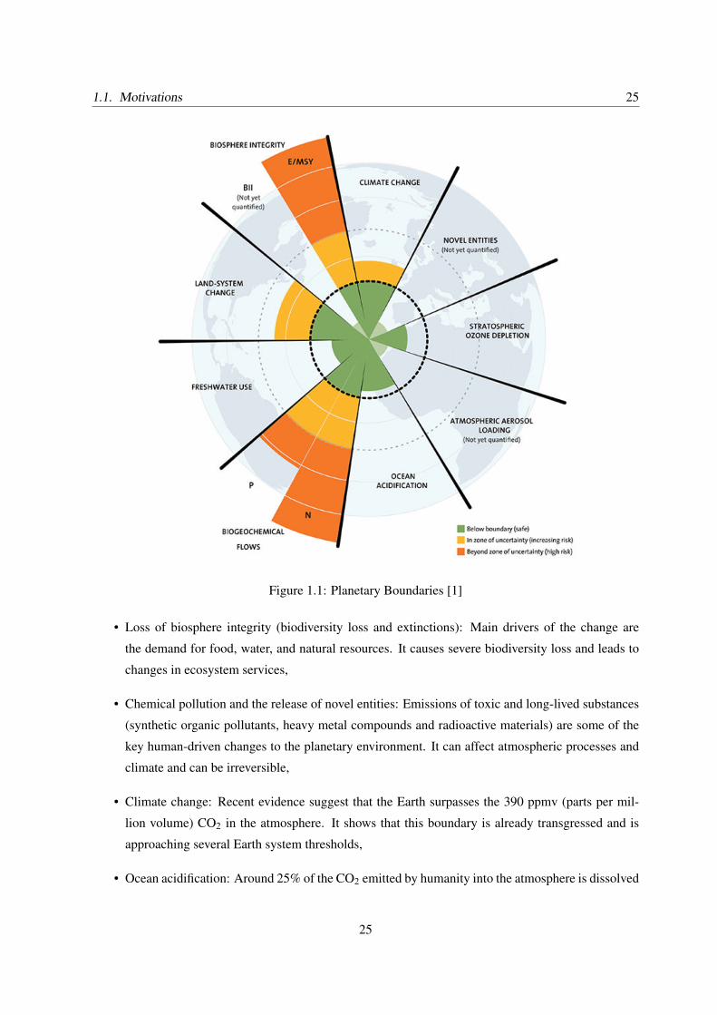
agriculture affects at least four out of nine planetary boundaries. Planetary boundaries and their current
values are presented in Figure 1.1 and defined according to [1].
• Stratospheric ozone depletion: The stratospheric ozone layer filters out ultraviolet (UV) radiation
from the sun. If UV radiation is not filtered, because the ozone layer decreased, it will reach the
ground level causing skin cancer in humans and damaging the terrestrial and marine biological
systems,
24
1.1. Motivations 25
Figure 1.1: Planetary Boundaries [1]
• Loss of biosphere integrity (biodiversity loss and extinctions): Main drivers of the change are
the demand for food, water, and natural resources. It causes severe biodiversity loss and leads to
changes in ecosystem services,
• Chemical pollution and the release of novel entities: Emissions of toxic and long-lived substances
(synthetic organic pollutants, heavy metal compounds and radioactive materials) are some of the
key human-driven changes to the planetary environment. It can affect atmospheric processes and
climate and can be irreversible,
• Climate change: Recent evidence suggest that the Earth surpasses the 390 ppmv (parts per mil-
lion volume) CO2 in the atmosphere. It shows that this boundary is already transgressed and is
approaching several Earth system thresholds,
• Ocean acidification: Around 25% of the CO2 emitted by humanity into the atmosphere is dissolved
25
26 Chapter 1. IoT and Smart Agriculture
in the oceans. Being in the ocean it forms carbonic acid, altering ocean chemistry and decreasing
the pH of the surface. Acidity reduces the available carbonate ions, which is essential for many
marine species for shell and skeleton formation,
• Freshwater consumption and the global hydrological cycle: This cycle is strongly affected by cli-
mate change and its boundary is linked to the climate boundary. Human pressure is the main
driving force determining the functioning and distribution of freshwater systems. Water is becom-
ing a scarce resource. It is estimated that by 2050 some 52% of the world population will live in
water-stressed regions [18],
• Land system change: Land is converted to human use around the planet. Forests, grasslands,
wetlands and other vegetation types have been converted to agricultural land. This change is one
of the main driving force of the reduction in biodiversity and it is impacting water flows and the
cycle of carbon, nitrogen and phosphorous among other important elements,
• Nitrogen and phosphorus flows to the biosphere and oceans: These two elements are essential for
plant growth and farmers use fertilizers to add those elements to the crops affecting the biochemical
cycles of them,
• Atmospheric aerosol loading: It influences the Earth’s climate system. When they interact with
water vapour, they affect the hydrological cycle impacting cloud formation and global-scale and
regional patterns of atmospheric circulation. They also affect climate as they change the reflection
and absorption of solar radiation in the atmosphere.
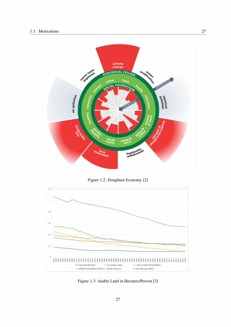
Going deeper in this topic, I also found an economic theory that not only includes the planetary bound-
aries I already mentioned, but also the UN Sustainable Development Goals (SDG) [19]. This economic
work, created by Kate Raworth, is very well described in her book "Doughnut Economy: Seven Ways
to Think Like a 21st-Century Economist" [2]. Raworth proposes that all economic considerations and
growths should be inside the two borders of the doughnut. The upper limit, ecological ceiling, is given
by the planetary boundaries, while the lower limit, social foundation, is provided by the UN SDGs. Fig-
ure 1.2 shows how the doughnut is configured in Raworth theory. Agriculture should also follow the
doughnut principle.
Finally, I found that we are facing a decrease in arable land as cities are growing, so there is less and
less land to be used by agriculture. According to FAO, the arable land at the beginning of the 1960s was
almost 0.5 ha/person. Nowadays, it is only 0.2 ha/person. Figure 1.3 presents the arable land in hectares
in different regions of the world from 1961 to 2018. It depicts how the arable land has been decreasing
in the last 50 years.
26
1.1. Motivations 27
Figure 1.2: Doughnut Economy [2]
Figure 1.3: Arable Land in Hectares/Person [3]
27
28 Chapter 1. IoT and Smart Agriculture
The humanity and the agriculture are facing an enormous dilemma: How to feed a growing population
having less land to grow crops, meeting the food security goals defined by UN FAO, and keeping plane-
tary boundaries in the safety zone?
I consider that this problem is an interesting challenge for electronics and information technologies: In-
ternet of Things (IoT) came immediately to my mind as well as Precision Agriculture (PA) based on
Automated Decision-Making Systems (ADMS). I started to look at different systems that are already
available in the market and how they are used. At that moment, I found that more than 80% of the
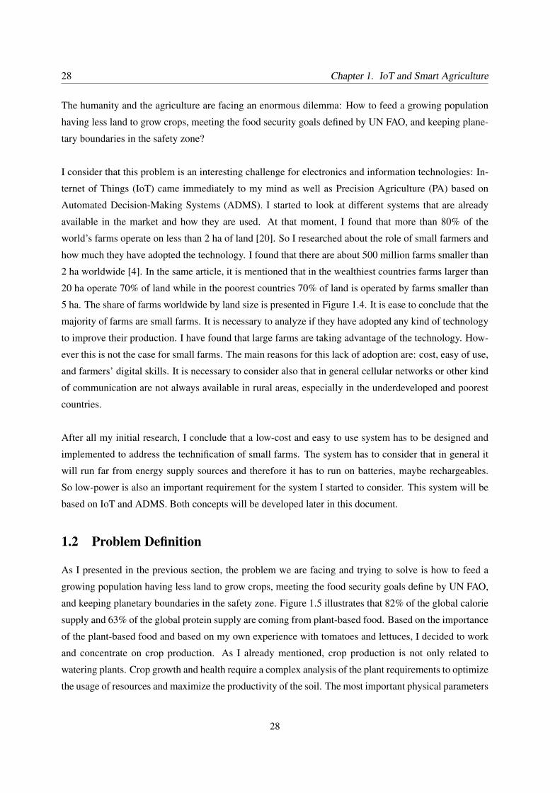
world’s farms operate on less than 2 ha of land [20]. So I researched about the role of small farmers and
how much they have adopted the technology. I found that there are about 500 million farms smaller than
2 ha worldwide [4]. In the same article, it is mentioned that in the wealthiest countries farms larger than
20 ha operate 70% of land while in the poorest countries 70% of land is operated by farms smaller than
5 ha. The share of farms worldwide by land size is presented in Figure 1.4. It is ease to conclude that the
majority of farms are small farms. It is necessary to analyze if they have adopted any kind of technology
to improve their production. I have found that large farms are taking advantage of the technology. How-
ever this is not the case for small farms. The main reasons for this lack of adoption are: cost, easy of use,
and farmers’ digital skills. It is necessary to consider also that in general cellular networks or other kind
of communication are not always available in rural areas, especially in the underdeveloped and poorest
countries.
After all my initial research, I conclude that a low-cost and easy to use system has to be designed and
implemented to address the technification of small farms. The system has to consider that in general it
will run far from energy supply sources and therefore it has to run on batteries, maybe rechargeables.
So low-power is also an important requirement for the system I started to consider. This system will be
based on IoT and ADMS. Both concepts will be developed later in this document.
1.2 Problem Definition
As I presented in the previous section, the problem we are facing and trying to solve is how to feed a
growing population having less land to grow crops, meeting the food security goals define by UN FAO,
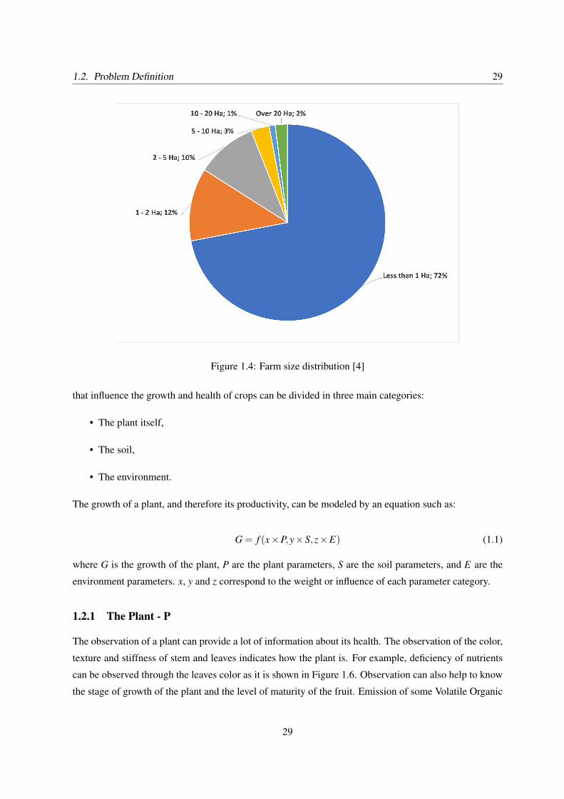
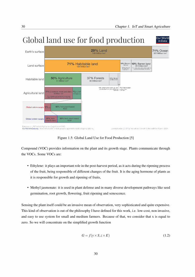
and keeping planetary boundaries in the safety zone. Figure 1.5 illustrates that 82% of the global calorie
supply and 63% of the global protein supply are coming from plant-based food. Based on the importance
of the plant-based food and based on my own experience with tomatoes and lettuces, I decided to work
and concentrate on crop production. As I already mentioned, crop production is not only related to
watering plants. Crop growth and health require a complex analysis of the plant requirements to optimize
the usage of resources and maximize the productivity of the soil. The most important physical parameters
28
1.2. Problem Definition 29
Figure 1.4: Farm size distribution [4]
that influence the growth and health of crops can be divided in three main categories:
• The plant itself,
• The soil,
• The environment.
The growth of a plant, and therefore its productivity, can be modeled by an equation such as:
G = f (x×P,y×S,z×E) (1.1)
where G is the growth of the plant, P are the plant parameters, S are the soil parameters, and E are the
environment parameters. x, y and z correspond to the weight or influence of each parameter category.
1.2.1 The Plant - P
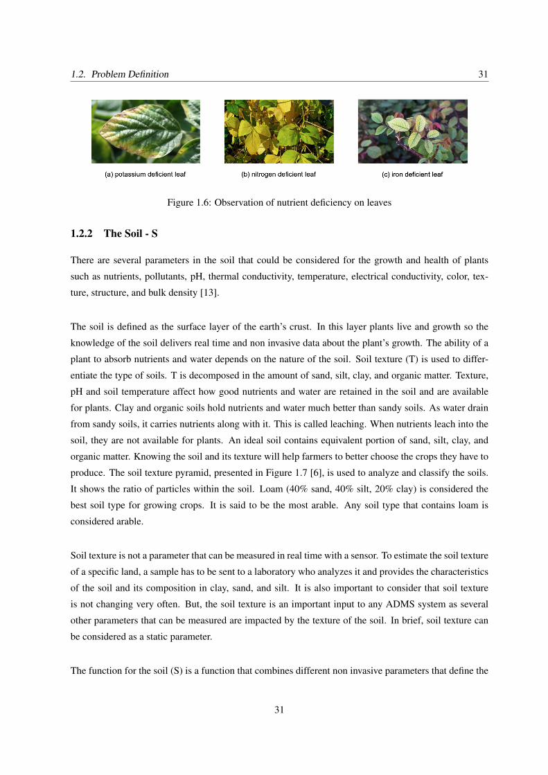
The observation of a plant can provide a lot of information about its health. The observation of the color,
texture and stiffness of stem and leaves indicates how the plant is. For example, deficiency of nutrients
can be observed through the leaves color as it is shown in Figure 1.6. Observation can also help to know
the stage of growth of the plant and the level of maturity of the fruit. Emission of some Volatile Organic
29
30 Chapter 1. IoT and Smart Agriculture
Figure 1.5: Global Land Use for Food Production [5]
Compound (VOC) provides information on the plant and its growth stage. Plants communicate through
the VOCs. Some VOCs are:
• Ethylene: it plays an important role in the post-harvest period, as it acts during the ripening process
of the fruit, being responsible of different changes of the fruit. It is the aging hormone of plants as
it is responsible for growth and ripening of fruits,
• Methyl jasmonate: it is used in plant defense and in many diverse development pathways like seed
germination, root growth, flowering, fruit ripening and senescence.
Sensing the plant itself could be an invasive mean of observation, very sophisticated and quite expensive.
This kind of observation is out of the philosophy I have defined for this work, i.e. low-cost, non invasive,
and easy to use system for small and medium farmers. Because of that, we consider that x is equal to
zero. So we will concentrate on the simplified growth function
G = f (y×S,z×E) (1.2)
30
1.2. Problem Definition 31
Figure 1.6: Observation of nutrient deficiency on leaves
1.2.2 The Soil - S
There are several parameters in the soil that could be considered for the growth and health of plants
such as nutrients, pollutants, pH, thermal conductivity, temperature, electrical conductivity, color, tex-
ture, structure, and bulk density [13].
The soil is defined as the surface layer of the earth’s crust. In this layer plants live and growth so the
knowledge of the soil delivers real time and non invasive data about the plant’s growth. The ability of a
plant to absorb nutrients and water depends on the nature of the soil. Soil texture (T) is used to differ-
entiate the type of soils. T is decomposed in the amount of sand, silt, clay, and organic matter. Texture,
pH and soil temperature affect how good nutrients and water are retained in the soil and are available
for plants. Clay and organic soils hold nutrients and water much better than sandy soils. As water drain
from sandy soils, it carries nutrients along with it. This is called leaching. When nutrients leach into the
soil, they are not available for plants. An ideal soil contains equivalent portion of sand, silt, clay, and
organic matter. Knowing the soil and its texture will help farmers to better choose the crops they have to
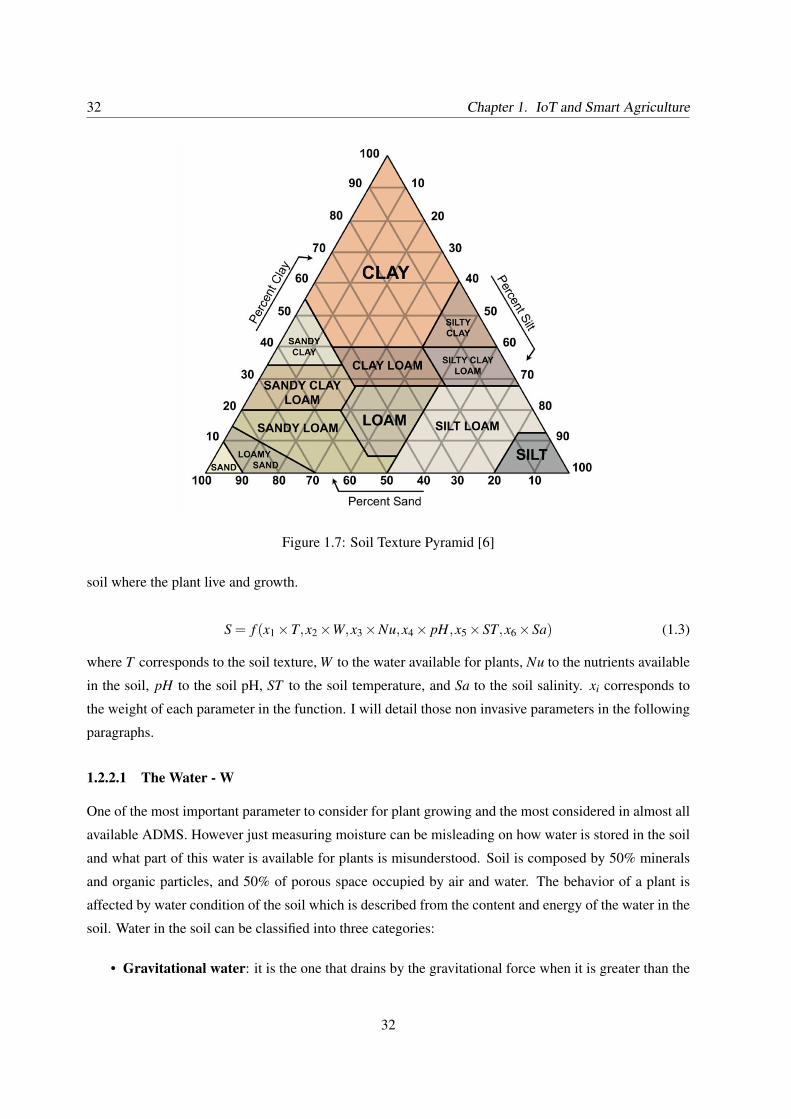
produce. The soil texture pyramid, presented in Figure 1.7 [6], is used to analyze and classify the soils.
It shows the ratio of particles within the soil. Loam (40% sand, 40% silt, 20% clay) is considered the
best soil type for growing crops. It is said to be the most arable. Any soil type that contains loam is
considered arable.
Soil texture is not a parameter that can be measured in real time with a sensor. To estimate the soil texture
of a specific land, a sample has to be sent to a laboratory who analyzes it and provides the characteristics
of the soil and its composition in clay, sand, and silt. It is also important to consider that soil texture
is not changing very often. But, the soil texture is an important input to any ADMS system as several
other parameters that can be measured are impacted by the texture of the soil. In brief, soil texture can
be considered as a static parameter.
The function for the soil (S) is a function that combines different non invasive parameters that define the
31
32 Chapter 1. IoT and Smart Agriculture
Figure 1.7: Soil Texture Pyramid [6]
soil where the plant live and growth.
S = f (x1 ×T,x2 ×W,x3 ×Nu,x4 × pH,x5 ×ST,x6 ×Sa) (1.3)
where T corresponds to the soil texture, W to the water available for plants, Nu to the nutrients available
in the soil, pH to the soil pH, ST to the soil temperature, and Sa to the soil salinity. xi corresponds to
the weight of each parameter in the function. I will detail those non invasive parameters in the following
paragraphs.
1.2.2.1 The Water - W
One of the most important parameter to consider for plant growing and the most considered in almost all
available ADMS. However just measuring moisture can be misleading on how water is stored in the soil
and what part of this water is available for plants is misunderstood. Soil is composed by 50% minerals
and organic particles, and 50% of porous space occupied by air and water. The behavior of a plant is
affected by water condition of the soil which is described from the content and energy of the water in the
soil. Water in the soil can be classified into three categories:
• Gravitational water: it is the one that drains by the gravitational force when it is greater than the
32
1.2. Problem Definition 33
Figure 1.8: Capillaries Forces
soil retention force. The value of this force is determined by the diameter of the porous. The plants
can absorb this water; however, it is not available for long time.
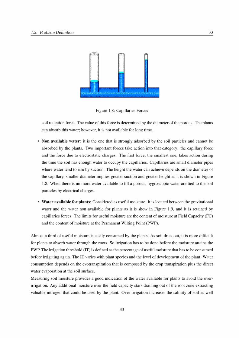
• Non available water: it is the one that is strongly adsorbed by the soil particles and cannot be
absorbed by the plants. Two important forces take action into that category: the capillary force
and the force due to electrostatic charges. The first force, the smallest one, takes action during
the time the soil has enough water to occupy the capillaries. Capillaries are small diameter pipes
where water tend to rise by suction. The height the water can achieve depends on the diameter of
the capillary, smaller diameter implies greater suction and greater height as it is shown in Figure
1.8. When there is no more water available to fill a porous, hygroscopic water are tied to the soil
particles by electrical charges.
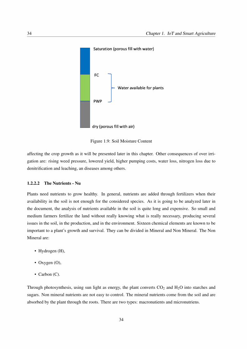
• Water available for plants: Considered as useful moisture. It is located between the gravitational
water and the water non available for plants as it is show in Figure 1.9, and it is retained by
capillaries forces. The limits for useful moisture are the content of moisture at Field Capacity (FC)
and the content of moisture at the Permanent Wilting Point (PWP).
Almost a third of useful moisture is easily consumed by the plants. As soil dries out, it is more difficult
for plants to absorb water through the roots. So irrigation has to be done before the moisture attains the
PWP. The irrigation threshold (IT) is defined as the percentage of useful moisture that has to be consumed
before irrigating again. The IT varies with plant species and the level of development of the plant. Water
consumption depends on the evotranspiration that is composed by the crop transpiration plus the direct
water evaporation at the soil surface.
Measuring soil moisture provides a good indication of the water available for plants to avoid the over-
irrigation. Any additional moisture over the field capacity stars draining out of the root zone extracting
valuable nitrogen that could be used by the plant. Over irrigation increases the salinity of soil as well
33
34 Chapter 1. IoT and Smart Agriculture
Figure 1.9: Soil Moisture Content
affecting the crop growth as it will be presented later in this chapter. Other consequences of over irri-
gation are: rising weed pressure, lowered yield, higher pumping costs, water loss, nitrogen loss due to
denitrification and leaching, an diseases among others.
1.2.2.2 The Nutrients - Nu
Plants need nutrients to grow healthy. In general, nutrients are added through fertilizers when their
availability in the soil is not enough for the considered species. As it is going to be analyzed later in
the document, the analysis of nutrients available in the soil is quite long and expensive. So small and
medium farmers fertilize the land without really knowing what is really necessary, producing several
issues in the soil, in the production, and in the environment. Sixteen chemical elements are known to be
important to a plant’s growth and survival. They can be divided in Mineral and Non Mineral. The Non
Mineral are:
• Hydrogen (H),
• Oxygen (O),
• Carbon (C).
Through photosynthesis, using sun light as energy, the plant converts CO2 and H2O into starches and
sugars. Non mineral nutrients are not easy to control. The mineral nutrients come from the soil and are
absorbed by the plant through the roots. There are two types: macronutients and micronutriens.
34
1.2. Problem Definition 35
• Macronutrients,
– Primary: Nitrogen (N), Phosphorous (P), and Potassium (K),
– Secondary: Calcium (Ca), Magnesium (Mg), and Sulfur (S).
• Micronutrients: Boron (B), Copper (Cu), Iron (Fe), Chloride (Cl), Manganese (Mn), Molybdenum
(Mo), and Zinc (Zn).
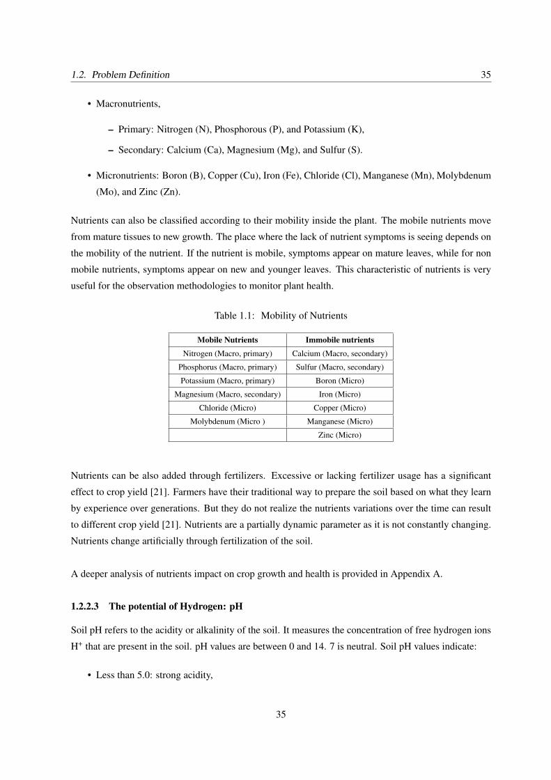
Nutrients can also be classified according to their mobility inside the plant. The mobile nutrients move
from mature tissues to new growth. The place where the lack of nutrient symptoms is seeing depends on
the mobility of the nutrient. If the nutrient is mobile, symptoms appear on mature leaves, while for non
mobile nutrients, symptoms appear on new and younger leaves. This characteristic of nutrients is very
useful for the observation methodologies to monitor plant health.
Table 1.1: Mobility of Nutrients
Mobile Nutrients Immobile nutrients
Nitrogen (Macro, primary) Calcium (Macro, secondary)
Phosphorus (Macro, primary) Sulfur (Macro, secondary)
Potassium (Macro, primary) Boron (Micro)
Magnesium (Macro, secondary) Iron (Micro)
Chloride (Micro) Copper (Micro)
Molybdenum (Micro ) Manganese (Micro)
Zinc (Micro)
Nutrients can be also added through fertilizers. Excessive or lacking fertilizer usage has a significant
effect to crop yield [21]. Farmers have their traditional way to prepare the soil based on what they learn
by experience over generations. But they do not realize the nutrients variations over the time can result
to different crop yield [21]. Nutrients are a partially dynamic parameter as it is not constantly changing.
Nutrients change artificially through fertilization of the soil.
A deeper analysis of nutrients impact on crop growth and health is provided in Appendix A.
1.2.2.3 The potential of Hydrogen: pH
Soil pH refers to the acidity or alkalinity of the soil. It measures the concentration of free hydrogen ions
H+ that are present in the soil. pH values are between 0 and 14. 7 is neutral. Soil pH values indicate:
• Less than 5.0: strong acidity,
35
36 Chapter 1. IoT and Smart Agriculture
• Between 5.0 and 6.0: moderate acidity,
• Between 6.5 and 7.5: neutral,
• Between 7.5 and 8.5: moderate alkalinity,
• Over than 8.5: strong alkalinity.
The pH scale was created to simplify the expression of H+. pH corresponds to the logarithm of the
reciprocal of the H+.
pH =−log(H+)
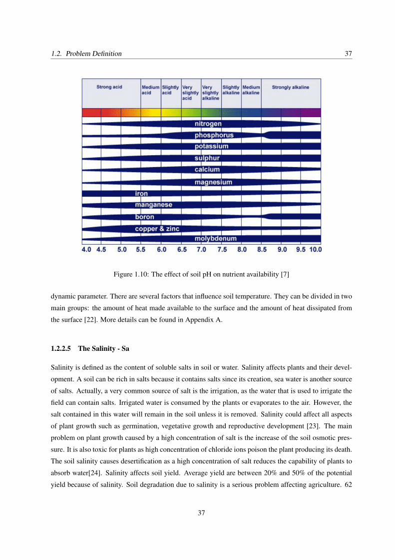
Soil pH outside the neutral range impacts the availability of nutrients. The pH is one of the most im-
portant soil properties that affects the availability of nutrients. pH is of great importance to plant roots
and microbial activity. Macronutrients tend to be less available in soil with low pH, i.e. more acid soils.
Micronutrients tend to be less available in soils with high pH, i.e. more alkaline soils. Additionally, pH
can also affects soil bacteria, nutrient leaching, toxic elements, and soil structure. For example, plant
nutrients leach out of soils with strong acidity much more rapidly than neutral pH soils. Aluminum may
become toxic in certain soils that have a strong acidity (below 5.0). pH is not an indication of fertility
but it affects the availability of nutrients as it is indicated in Figure 1.10. Suitable pH value depends on
species. For example blueberries need a more acid soil than tomatoes.
pH is a partially dynamic parameter as it can change with the rain and/or with the irrigation.
1.2.2.4 The Soil Temperature - ST
Soil is a major storage for heat. It behaves as a reservoir that stores energy during the day and as a source
that displays heat to the surface during the night. Soil temperature governs:
• Physical processes,
• Chemical processes,
• Biological processes.
The amount of received radiation affects soil temperature and some biological processes such as seed
germination, seedling emergence, plant root growth, and nutrient availability [22]. The soil temperature
modifies the rate of organic matter decomposition and the mineralization of organic materials in the soil.
It also affects water retention, transmission, and availability to plants. It is a function of the heat flux and
heat exchanges between soil and atmosphere, with seasonal daily variation. Soil temperature is a fully
36
1.2. Problem Definition 37
Figure 1.10: The effect of soil pH on nutrient availability [7]
dynamic parameter. There are several factors that influence soil temperature. They can be divided in two
main groups: the amount of heat made available to the surface and the amount of heat dissipated from
the surface [22]. More details can be found in Appendix A.
1.2.2.5 The Salinity - Sa
Salinity is defined as the content of soluble salts in soil or water. Salinity affects plants and their devel-
opment. A soil can be rich in salts because it contains salts since its creation, sea water is another source
of salts. Actually, a very common source of salt is the irrigation, as the water that is used to irrigate the
field can contain salts. Irrigated water is consumed by the plants or evaporates to the air. However, the
salt contained in this water will remain in the soil unless it is removed. Salinity could affect all aspects
of plant growth such as germination, vegetative growth and reproductive development [23]. The main
problem on plant growth caused by a high concentration of salt is the increase of the soil osmotic pres-
sure. It is also toxic for plants as high concentration of chloride ions poison the plant producing its death.
The soil salinity causes desertification as a high concentration of salt reduces the capability of plants to
absorb water[24]. Salinity affects soil yield. Average yield are between 20% and 50% of the potential
yield because of salinity. Soil degradation due to salinity is a serious problem affecting agriculture. 62
37
38 Chapter 1. IoT and Smart Agriculture
millions ha are affected by salinity worldwide [25].
Salinity is a partially dynamic parameter as it can change with the rain and/or with the irrigation. There
are two types of salinity:
• Natural salinity (primary): Caused by natural processes (salt deposition caused by rain, rock degra-
dation and dissolution of minerals, and groundwater rising to the surface by capillarity,
• Secondary salinity: Caused by humans (irrigation management, irrigation with saline water, fer-
tilisers application, and inadequate drainage conditions.
1.2.3 The Environment - E
Plants grow also on environmental characteristics. The function of the environment (E) depends on
several parameters that define the place where the plant grows.
E = f (x1 ∗L,x2 ∗ET,x3 ∗We,x3 ∗Rh)
where L corresponds to the light captured by the plant, ET corresponds to the environment temperature,
We to the weather, and Rh to the air relative humidity. xi correspond to the weight of each parameter in
the function.
1.2.3.1 The Light - L
Plants use light, water, and carbon dioxide (CO2) to produce sugar, which is converted to ATP (Adenosine
5’-triphosphate) by cellular respiration. This conversion is made through photosynthesis. Charles Darwin
defined the light effect on plants as "Heliotropism prevails so extensively among the higher plants, that
there are extremely few, of which some part, either the stem, flower-peduncle, petiole, or leaf, does not
bend towards a lateral light" [26].
Light is a fully dynamic parameter and can be artificially changed only on greenhouses. Light is mainly
sun light except when greenhouses are considered, using artificial means to produce the light needed by
plants. The light features are: light quantity, light quality, and light duration [27]. More details can be
found in Appendix A.
1.2.3.2 Environmental Temperature
Rate of plant growth and development is dependent upon the temperature surrounding the plant. Each
species has a specific temperature range represented by a minimum, maximum, and optimum. Environ-
mental temperature is one of the most important factors of plant development. With climate change, it is
38
1.2. Problem Definition 39
expected that extreme temperatures will be faced more often, affecting plant productivity.
Pollination is one of the stages of phenology most sensitive to temperature extremes in all species. Tem-
perature extremes would significantly affect productivity [28]. Water deficit and excess water in the soil
increase the effects of temperature. For that reason, it is very important to understand the interaction
of temperature and water to develop more effective adaptation strategies to face the impact of greater
temperatures. A review from Barlow et al. [29] on the effect of extreme temperatures in wheat showed
that frost caused sterility and abortion of formed grains, while heat caused reduction in grain number and
reduced the duration of the grain filling period.
Environmental temperature is a fully dynamic parameter. It can be artificially modified.
1.2.3.3 The Weather - We
The weather plays a major role on crop growth and it has to be monitored periodically. So farmers can act
if weather conditions are not convenient for the crops they have. For instance, heavy rain, hail or storms
in summer can affect tomato production. Morning frost can affect the production of fruits if they happen
during the flowering of trees. Strong winds may affect the production of fruits during the flowering of
trees. Very high temperatures can affect lettuce production.
Consequences of extreme weather cannot be handled by an ADMS system. However knowing them in
advance could produce alarms to the farmer so mitigation actions can be taken on time.
Weather is a fully dynamic parameter and cannot be artificially modified except in greenhouses.
1.2.3.4 Air Relative Humidity - Rh
[30] states that "Relative humidity is the amount of water vapor in the air relative to the maximum amount
of vapor water that the air can hold at a certain temperature." The level of relative humidity affects when
and how plants open the stomata on the leaves. Stomata is used by plants to transpire (breathe). On
warm weathers plants may close the stomata to reduce the water losses. Stomata also act as a cooling
mechanism.
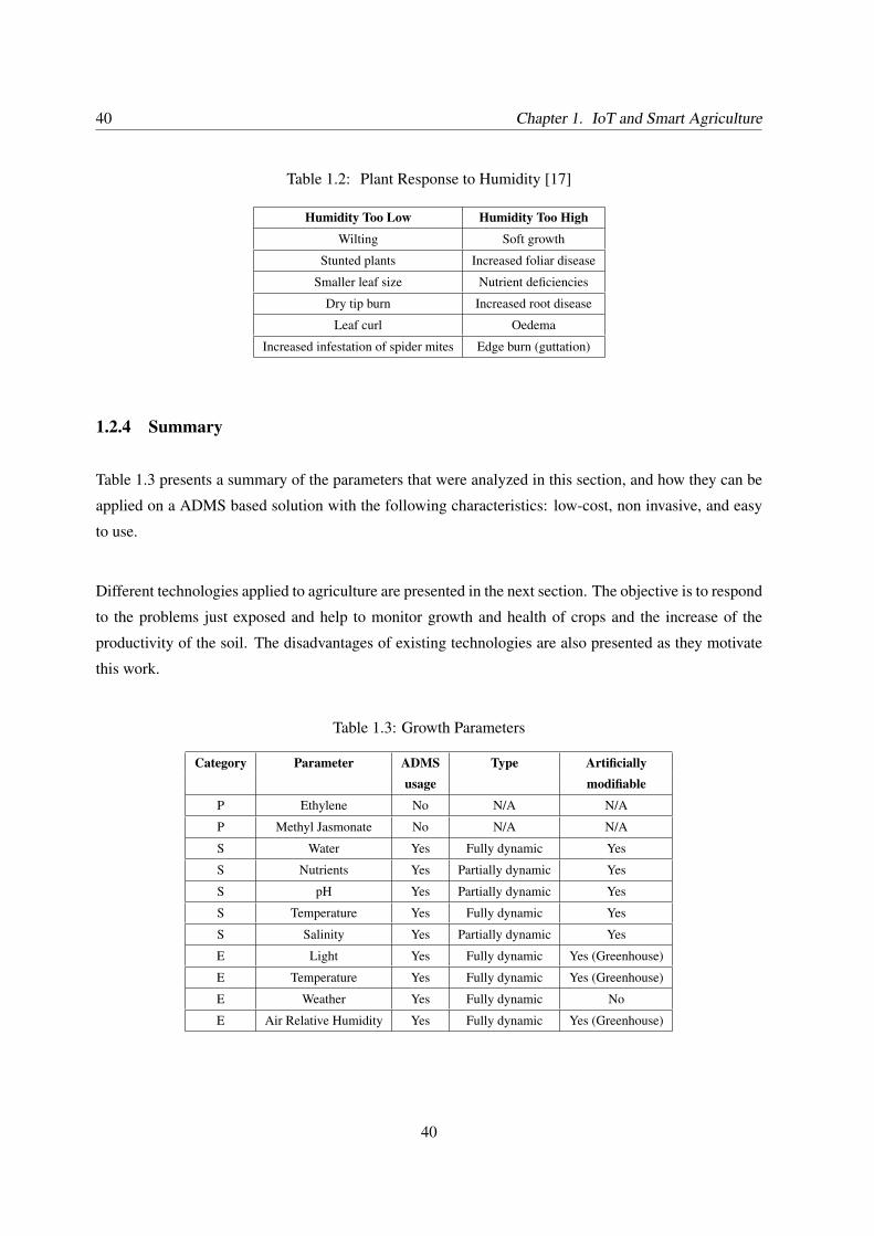
Plants respond in different ways to humidity. Table 1.2 summarizes different plants reaction to humidity.
Air relative humidity is a fully dynamic parameter and cannot be artificially modified except in green-
houses.
39
40 Chapter 1. IoT and Smart Agriculture
Table 1.2: Plant Response to Humidity [17]
Humidity Too Low Humidity Too High
Wilting Soft growth
Stunted plants Increased foliar disease
Smaller leaf size Nutrient deficiencies
Dry tip burn Increased root disease
Leaf curl Oedema
Increased infestation of spider mites Edge burn (guttation)
1.2.4 Summary
Table 1.3 presents a summary of the parameters that were analyzed in this section, and how they can be
applied on a ADMS based solution with the following characteristics: low-cost, non invasive, and easy
to use.
Different technologies applied to agriculture are presented in the next section. The objective is to respond
to the problems just exposed and help to monitor growth and health of crops and the increase of the
productivity of the soil. The disadvantages of existing technologies are also presented as they motivate
this work.
Table 1.3: Growth Parameters
Category Parameter ADMS Type Artificiallyusage modifiable
P Ethylene No N/A N/A
P Methyl Jasmonate No N/A N/A
S Water Yes Fully dynamic Yes
S Nutrients Yes Partially dynamic Yes
S pH Yes Partially dynamic Yes
S Temperature Yes Fully dynamic Yes
S Salinity Yes Partially dynamic Yes
E Light Yes Fully dynamic Yes (Greenhouse)
E Temperature Yes Fully dynamic Yes (Greenhouse)
E Weather Yes Fully dynamic No
E Air Relative Humidity Yes Fully dynamic Yes (Greenhouse)
40
1.3. Technologies for Agriculture 41
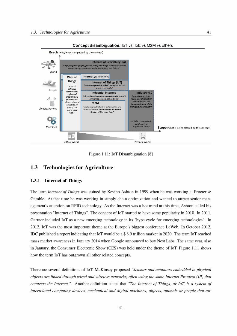
Figure 1.11: IoT Disambiguation [8]
1.3 Technologies for Agriculture
1.3.1 Internet of Things
The term Internet of Things was coined by Kevinh Ashton in 1999 when he was working at Procter &
Gamble. At that time he was working in supply chain optimization and wanted to attract senior man-
agement’s attention on RFID technology. As the Internet was a hot trend at this time, Ashton called his
presentation "Internet of Things". The concept of IoT started to have some popularity in 2010. In 2011,
Gartner included IoT as a new emerging technology in its "hype cycle for emerging technologies". In
2012, IoT was the most important theme at the Europe’s biggest conference LeWeb. In October 2012,
IDC published a report indicating that IoT would be a $ 8.9 trillion market in 2020. The term IoT reached
mass market awareness in January 2014 when Google announced to buy Nest Labs. The same year, also
in January, the Consumer Electronic Show (CES) was held under the theme of IoT. Figure 1.11 shows
how the term IoT has outgrown all other related concepts.
There are several definitions of IoT. McKinsey proposed "Sensors and actuators embedded in physical
objects are linked through wired and wireless networks, often using the same Internet Protocol (IP) that
connects the Internet.". Another definition states that "The Internet of Things, or IoT, is a system of
interrelated computing devices, mechanical and digital machines, objects, animals or people that are
41
42 Chapter 1. IoT and Smart Agriculture
provided with unique identifiers and the ability to transfer data over a network without requiring human-
to-human or human-to-computer interaction." [31]. It can also be stated that the IoT is the network of
physical devices, vehicles, home appliances, and other items embedded with electronics, software, sen-
sors, actuators, and network connectivity. It enables these objects to collect and exchange data. Each
“thing” is uniquely identifiable through its embedded computing system but is able to interoperate within
the existing Internet infrastructure.
The IoT allows objects to be sensed or controlled remotely across a public or private network infras-
tructure, creating opportunities for more direct integration of the physical world into computer-based
systems, and resulting in improved efficiency, accuracy and economic benefit in addition to reduced
human intervention. When IoT is augmented with sensors and actuators, the technology becomes an
instance of the more general class of cyber-physical systems, which also encompasses technologies such
as smart grids, virtual power plants, smart homes, intelligent transportation and smart cities. "Things", in
the IoT sense, can refer to a wide variety of devices such as heart monitoring implants, biochip transpon-
ders on farm animals, cameras streaming live feeds of wild animals in coastal waters, automobiles with
built-in sensors, DNA analysis devices for environmental/food/pathogen monitoring, or field operation
devices that assist firefighters in search and rescue operations. Legal scholars suggest regarding "things"
as an "inextricable mixture of hardware, software, data and service". These devices collect useful data
with the help of various existing technologies and then autonomously flow the data between other de-
vices. The quick expansion of Internet-connected objects is also expected to generate large amounts of
data from diverse locations, with the consequent necessity for quick aggregation of the data. So better
and more efficient methodologies and algorithms to index, store, and process such data will be necessary.
“IoT is no longer just the next phase of the Internet — it’s fundamentally reshaping the core character-
istics of the internet as we know it.” [32]. According to Maciej Kranz [32], IoT changes are impacting
the core characteristics of the Internet, and is touching several business domains such as agricultural and
environmental with several applications: smart irrigation and fertilization, smart lighting in nesting or
poultry farming, livestock health and asset tracking, preventative maintenance on remote farming equip-
ment, drone-based land surveys, farm-to-market supply chain efficiencies with asset tracking, robotic
farming, and volcanic and fault line monitoring for predictive disasters. Smart irrigation and fertilization
will be analyzed as part of this work.
Masayoshi Son, Chairman and CEO of SoftBank Group and Chairman of Arm Holdings, said that more
than a trillion of IoT devices will be built between 2017 and 2035. In 2015, report form Harvard Business
Review [33] there will be not a single industry that won’t benefit from the IoT.
42
1.3. Technologies for Agriculture 43
Figure 1.12: IoT Architecture [9]
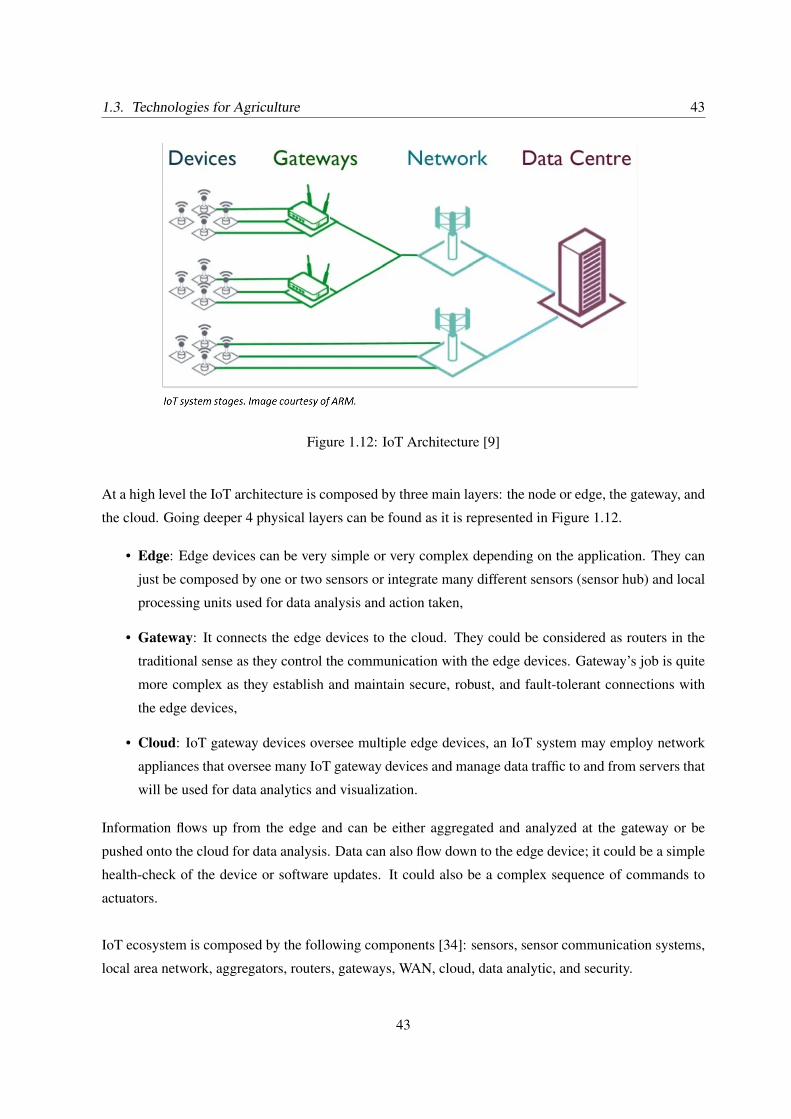
At a high level the IoT architecture is composed by three main layers: the node or edge, the gateway, and
the cloud. Going deeper 4 physical layers can be found as it is represented in Figure 1.12.
• Edge: Edge devices can be very simple or very complex depending on the application. They can
just be composed by one or two sensors or integrate many different sensors (sensor hub) and local
processing units used for data analysis and action taken,
• Gateway: It connects the edge devices to the cloud. They could be considered as routers in the
traditional sense as they control the communication with the edge devices. Gateway’s job is quite
more complex as they establish and maintain secure, robust, and fault-tolerant connections with
the edge devices,
• Cloud: IoT gateway devices oversee multiple edge devices, an IoT system may employ network
appliances that oversee many IoT gateway devices and manage data traffic to and from servers that
will be used for data analytics and visualization.
Information flows up from the edge and can be either aggregated and analyzed at the gateway or be
pushed onto the cloud for data analysis. Data can also flow down to the edge device; it could be a simple
health-check of the device or software updates. It could also be a complex sequence of commands to
actuators.
IoT ecosystem is composed by the following components [34]: sensors, sensor communication systems,
local area network, aggregators, routers, gateways, WAN, cloud, data analytic, and security.
43
44 Chapter 1. IoT and Smart Agriculture
An important topic to consider when analyzing IoT is the edge computing which considers that data is
stored and processed on or as close as possible to the device generating the data [35]. Gartner estimates
that the percentage of enterprise-generated-data created and processed outside of a traditional, centralized
data center will go from 10% in 2019 to 75% by 2025. One of the most important benefits of edge
computing is to process the data in real time. On the other hand, it eliminates the latency associated with
transmitting data over a network. Latency can be a showstopper for certain applications that request real
time processing. Also edge computing enables data processing in that be the case for agriculture.
1.3.2 Communication technology - LPWAN
In general, cellular communication is not available in rural areas or it is quite expensive to be considered
for a IoT system. Even in the developed countries the access to networks that can be used to transfer data
is not always available, in under developed countries the problem is even worst.
As a response to that issue, Low-Power Wide Area Network (LPWAN) emerged as a term, not as a new
technology standard in 2013. LPWAN is a class of wireless technologies suitable to the specific needs of
machine-to-machine and IoT devices [36].
LPWAN is a wireless wide area network used to interconnect low-bandwith, battery-powered devices
that transmit low bit rates over long ranges. It operates at a lower cost and greater power efficiency than
traditional mobile networks. They can support an important number of connected devices in a large area
[37].
LPWAN can work with packets from 10 to 1.000 bytes at uplink speeds up to 200 Kbps. The range can
go from 2 km to 1.000 km depending on the technology. Most of existing LPWAN technologies are
based on a star topology where each endpoint is connected to a common central point.
According to James Brehm & Associates, 86% of all IoT devices use less than 3 MB of data per month.
3rd Generation Partnership Project (3GPP) estimates that 99% of LPWAN devices consume or will con-
sume less than 150 KB of date per month [37]. Cellular networks have poor battery life and have gaps
in coverage. IoT devices are deployed for several years and for the case of agriculture in places where it
is hard to consider changing the battery, so low-power to keep the system alive is a must.
LPWAN technologies are used in several IoT applications including smart metering, smart lighting, asset
monitoring and tracking, smart cities, precision agriculture, livestock monitoring, energy management,
and others.
44
1.3. Technologies for Agriculture 45
There are several types of LPWAN. Moreover, they can be licensed or unlicensed. The most important
and most used LPWAN technologies are [37]:
• Sigfox: Proprietary and unlicensed. It is one of the most widely deployed nowadays. It runs
over a public network in the 868 MHz or 902 MHz band. It enables only a single operator per
country. Packet size is limited to 150 messages of 12 bytes per day. Messages can be delivered
over distances of 30-50 km. in rural areas, 3 - 10 km. in urban areas and up to 1.000 km. in
line-of-site applications. Downlink packets are limited to four messages of 8 bytes per day,
• Random phase multiple access (RPMA): Proprietary. It has a range up to 50 km. line of sight and
5 - 10 km. nonline of sight. It runs in the 2.4 GHz band so it can have interference with Wi-Fi,
Bluetooth, and physical structures. It is the one with the highest consumption,
• Long Range (LoRa): Unlicensed. Specified by the LoRa Alliance. It transmits in several sub-
gigahertz frequencies so it is less susceptible to interference. It allows user to define the packet size.
While open source, the transceiver chip is only available from Semtech Corporation. LoRaWAN
is the media access control layer protocol that manages the communication between devices and
the gateway,
• Weightless SIG: It has developed three LPWAN standards (Unidirectional Weightless-N, bidirec-
tional Weightless-P and Weightless-W). Weightless-N and Weightless-P are more popular as they
have a longer battery life than Weightless-W. Weightless-N and Weightless-P run in the sub-1 GHz
unlicensed spectrum. They also support a licensed spectrum operation at 12.5 kHz narrowband
technology,
• Narrowband-IoT (NB-IoT): Part of the 3GPP. It operates on the licensed spectrum on existing cel-
lular infrastructure. NB-IoT (CAT-NB1) operates on existing LTE and Global System for Mobile
(GSM) infrastructure. It offers uplink and downlink rates of 200 Kbps and it uses only 200 kHz of
available bandwidth,
• LTE-M: Also part of the 3GPP. It operates on the licensed spectrum on existing cellular infras-
tructure. LTE-M (CAT-M1) has higher bandwidth than NB-IoT, and the highest bandwidth of any
LPWAN technology.
• Other technologies: GreenOFDM from GreenWaves Technologies, DASH7 from Haystack Tech-
nologies Inc., Symphony Link from Link Labs Inc., ThingPark Wireless from Actility, Ultra Nar-
row Band from various companies including Telensa, Nwave and Sigfox, and WAVIoT.
45
46 Chapter 1. IoT and Smart Agriculture
1.3.3 State of the Art
PA enables to improve crop yields and to assist management decisions using high technology sensor and
analysis tools [38]. PA is a concept to increase production, reduce labor time, and ensure the effective
management of fertilizers and irrigation processes. PA is a management tool providing information to
the farmer to make better decisions.
Smart agriculture refers to the usage of technologies like IoT, sensors, location systems, robots and ar-
tificial intelligence on the farm. The ultimate goal is increasing the quality and quantity of the crops
while optimizing the human labor. Smart agriculture systems make decisions and act without human
intervention.
Several research have tried to model the growth of plants and it is important to mention the mathematical
model published by Gilad, Hardenberg, Provenzale, Shachak, and Meron [39] where a model for a single
plant with water as a limited resource is introduced. This model considers three dynamic variables, the
biomass density, the soil-water density, and the surface water. Hunt, Causton, Shipley and Askew [40]
presented a modern tool for classical plant analysis. Bessonov and Volpert provided a lot of information
about plant growth model in their book Dynamical Model of Plant Growth [41]. Another useful docu-
ment on plant growth modeling was produced by Fourcaud, Zhang, Stokes, Lambers, and Körner [42].
From all those models we can easily conclude that water is one of the most important factors for plants
growth.
Salinity remote measurement has also been a topic of research as sending samples to a specialized labo-
ratory is expensive and time consuming. Metternicht and Zinck presented an overview of various sensors
and approaches used for remote identification of areas affected by salinity [43].
IoT has been the selected technology to monitor and control plant irrigation according to an article pub-
lished by Romit Atta "At the turn of the century, none of the 525 million farms across the world had
sensor technology. Cut to 2025, and we will witness more than 620 million sensors being used”, “ al-
most 2 billion smart agro-sensors expected to be in active use by 2050”. In the same article it is also
stated "Between 2017 and 2022, the agricultural IoT market is set to expand at a mighty impressive
Compound Annual Growth Rate (CAGR) of around 16% - 17%" [44]. Romit Atta also states that “Lack
of power water management has been a long-standing bane of the primary sector." and continue "After
research we found that close to 60% of water released for agricultural gets wasted – due to overwatering,
runoffs, contamination, and other related issues”.
46
1.3. Technologies for Agriculture 47
Several IoT applications have been developed in countries where agriculture plays an important role in
the country economy, especially China and India. In general those systems make data capture by sen-
sors and data analysis in the cloud implying higher cost and higher power consumption. This approach
is relevant in places where connection to the internet is available. However, this is not the case in the
underdeveloped countries, where sending data to the cloud is almost infeasible. On the other hand, even
if the connection is available, the cost might make this solution as a non-practical one when considering
small and medium farmers.
Shareef and Viswanathan [45] present an agricultural monitoring system based on sensors and transfer-
ring the data to the cloud for processing using Light Fidelity (Li-Fi) technology. All data are processed
in the cloud and the system provides alarms and messages to farmers through a mobile application.
Namani and Gonen present an IoT system for smart agriculture based on drones and cloud computing
[46]. According to Namani and Gonen several autonomous technique are used to inspect the health
state of the farm. One of those techniques is the satellites that monitor the farm and record data that is
processed in the cloud. This technique is not convenient for small farms and the usage of drones can
substitute the satellite as they are more convenient and cheaper for small farmers. Namani and Gonen
state that drones in combination with IoT and cloud computing technologies, can help in real-time data
extraction, evaluation and solutions to the agricultural farming. In their solution Namani and Gonen
present a system based on drones that identifies pests, weeds and diseases of plants, estimates crop yield,
provides data on soil fertility, and measures irrigation.
Kassim presents the existing IoT applications in Precision Agriculture by defining 4 main domains [47]:
• Weather monitoring: Monitor critical weather parameters that impact the growth of crops including
temperature, humidity, wind, air pressure, etc. Data is collected by sensors and sent to the cloud
for analysis,
• Soil conditions monitoring: One of the most demanding practices. Parameters include soil humid-
ity, pH, moisture and temperature,
• Disease monitoring: Help farmers to make informed decisions. Image processing and machine
learning are used the the health of plants,
• Irrigation monitoring: Takes current weather and soil conditions in account. Irrigation is done only
when it is necessary.
Goap, Sharma, Shukla, and Krishna add the concept of machine learning to the IoT based irrigation
47
48 Chapter 1. IoT and Smart Agriculture
system presented at [48] to predict the irrigation requirements of a field using sensed data.
Dos Santos, Pessin, da Costa, and da Rosa Righi presented their system, AgriPrediction, that combines
a wireless network with a prediction engine to indicate potential crop issues [49].
It should be noted that the COVID pandemic has accelerated the use of Digital Agriculture as it is
presented by Arathoon, Raithatha and Tricarico in [50]. The key findings of this study are:
• COVID-19 has shown the necessity of a resilient and efficient agricultural value chain,
• The pandemic has shown the ability of digital tools to help smallholder farmers to overcome several
pain points, making them more resilient to future problems,
• The pandemic has accelerated the adoption of digital agriculture, however several points have
to be improved in the future: challenges related to availability and access to technology, digital
technology will increase the division between female and male farmers, and risk of misinformation
because of social media platforms usage.
Patidar, Khatri and Gurjar presented the design of an Application Specific Integrated Circuit (ASIC) for
PA and they made a test on a FPGA [51]. Another similar work was presented by Madhukar and Reddy
in their publication about a SoC for PA implemented on FPGA [52]. Regarding System on Chip (SoC)
or ASIC there is not too much literature as almost all research and industrial applications are prototypes
and built on platforms. Prototypes are made on Arduino and Raspberry Pi while products are made on
out-off-the shelf processors.
In this section, four main research topics have been presented: mathematical model of plant growth, IoT
and precision agriculture, machine learning and artificial intelligence in smart agriculture, and SoC for
smart agriculture.
For the first one, the mathematical model, I have analyzed several documents and I have found that so
far it is difficult to state that a model can represent the growth of plants. The problem is quite complex
and too many variables should be considered.
Regarding IoT and Precision Agriculture I have found a lot of material that show how sensors and sys-
tems can be used to improve the productivity of the soil. In general, the systems that I have studied
take in consideration one or two parameters and process in the cloud. Those systems help in same way
farmers to define when to irrigate based on the information they have, however the information is quite
incomplete and could recommend irrigation when it is not needed as not all parameters are analyzed by
48
1.4. My Contributions 49
the system.
The third one, machine learning and artificial intelligence, is more recent. The aim of those systems is
to be able to predict actions based on historical data and current conditions. They can predict irrigation
needs or health of the crops.
Finally, I have not found too much literature about SoC for precision agriculture, just a couple of papers
that present a FPGA solution. This is a topic that needs a lot of research and one of the reasons I decided
to design a SoC as part of my thesis.
1.4 My Contributions
After a deep analysis of the facts that motivate me to work on IoT for agriculture combined with current
world situation and the State of the Art, I have found that in general small and medium farmers are not
getting the attention they need: A system taking in account this important part of the agricultural produc-
tion is clearly necessary. Additionally, it is important to understand that the growth and health of plants
depend on several physical parameters, chemical parameters, and processes and measure just moisture is
not enough. Just measuring moisture can even conduct to over irrigation, creating more problems to the
plant.
Specific requirements have to be considered for crop production on small to medium farms:
• Low-power as the device has to work for at least 3 years far from any power supply,
• Able to process data at the edge as communications are not always available in the rural areas, and
even if they are, their cost can be prohibitive,
• Low-cost as small to medium farmers do not have the possibility to invest in technology. Their
production gives them just what they need to live in some cases,
• Easy to use as the target users do not have digital skills.
I decided to design an IoT system for crop monitoring to improve the productivity of the soil while keep-
ing the environment safe, which is the main objective of this thesis.
To accomplish these restrictions my system consists of:
• SoC,
49
50 Chapter 1. IoT and Smart Agriculture
• Peripherals I/Os (Analog-to-Digital Converter (ADC), Digital-to-analog converter (DAC), Pulse-
Width Modulation (PWM), Inter-Integrated Circuit (I2C), Serial Peripheral Interface (SPI), Uni-
versal Asynchronous Receiver-Transmitter (UART)),
• LoRa communication chip,
• Battery.
The system works on low-power and is able to:
• Get data from sensors connected through peripheral I/Os,
• Process data in the edge,
• Drive actuators connected through peripheral I/Os,
• Send information to the cloud for further analysis,
• Send analysis and/or results to the farmer.
As it was mentioned earlier, the system is designed for small to medium farmers. Low-cost is a require-
ment that is considered in all steps of the design of the system.
The document is organized as follows:
Chapter 2 presents how to measure the different parameters already analyzed and the available sen-
sors that can be used for this purpose. It also presents several experiments using the sensors that were
realized during my research work. As it will be detailed in the chapter, most of the experiments were
conducted at home because of the COVID pandemic.
Chapter 3 presents the SoC that was designed as part of this research work. Design flow, used IPs,
FPGA prototyping, and resulting layout are detailed in this chapter.
Chapter 4 presents the Smart Agriculture community I have created and the research activities we are
doing to bring technology to the farms to improve not only the productivity of the farm but also to
improve the life of the farmer and his family while keeping the planet safe.
50
CHAPTER
2HOW TO MEASURE
IMPORTANT PARAMETERS
FOR PLANT GROWTH AND
HEALTH
Sommaire2.1 Parameters Measurement . . . . . . . . . . . . . . . . . . . . . . . . . . . . . . . . 52
2.1.1 Measurement of Water . . . . . . . . . . . . . . . . . . . . . . . . . . . . . . 53
2.1.2 Measurement of Nutrients . . . . . . . . . . . . . . . . . . . . . . . . . . . . 55
2.1.3 Soil pH Measurement . . . . . . . . . . . . . . . . . . . . . . . . . . . . . . 58
2.1.4 Soil Temperature Measurement . . . . . . . . . . . . . . . . . . . . . . . . . 61
2.1.5 Soil Salinity Measurement . . . . . . . . . . . . . . . . . . . . . . . . . . . . 62
2.1.6 The Light . . . . . . . . . . . . . . . . . . . . . . . . . . . . . . . . . . . . . 63
2.1.7 The Weather . . . . . . . . . . . . . . . . . . . . . . . . . . . . . . . . . . . 63
2.1.8 Summary . . . . . . . . . . . . . . . . . . . . . . . . . . . . . . . . . . . . . 63
2.2 Experimental Laboratory at Home . . . . . . . . . . . . . . . . . . . . . . . . . . . 64
2.2.1 Experiment 1: Chives - Spring . . . . . . . . . . . . . . . . . . . . . . . . . . 64
2.2.2 Experiment 2 - Cherry tomatoes - Summer . . . . . . . . . . . . . . . . . . . 68
2.2.3 Experiment 3 - Cherry tomatoes - Summer . . . . . . . . . . . . . . . . . . . 72
2.2.4 Experiment 4 - Bell Pepper - End of Fall . . . . . . . . . . . . . . . . . . . . 74
2.3 Parameters Measurement and their Interrelation . . . . . . . . . . . . . . . . . . . 76
51
52 Chapter 2. How to Measure Important Parameters for Plant Growth and Health
In Chapter 1, the problem related to the growth and health of plants has been presented emphasizing
the role the technology can play to help small and medium farmers to improve their productivity while
keeping the planetary boundaries at a reasonable level. In this second chapter different methodologies
to measure the parameters presented in Chapter 1 and influencing the plant growth and health are
analyzed based on the requirements defined for this system: low-power, low-cost , easy-to-use, in-situ,
and real-time. Several experiments are also presented to validate several of the stated hypothesis and
the interrelation between parameters. A summary of the chosen methodologies and the available sensors
are discussed at the end of this chapter.
2.1 Parameters Measurement
Crop’s yield depends on physical parameters that have to be measured and controlled. Each of these
should be evaluated to determine whether it is relevant to be integrated into an IoT system for small and
medium-size farms based on the defined restrictions for this kind of systems:
• Ease of measurement: different options have to be analyzed for each parameter,
• Cost of the measurement: it has to be affordable for farmers, especially small to medium farmers,
• Timing of measurement: real-time or a given periodicity. The periodicity has to be analyzed by
testing different approaches per parameter to find a good trade-off between accuracy, power, and
measurement cost,
• Accuracy of measurement: sensors accuracy and positioning of sensors. Positioning and distance
between sensors will be analysed in the future, once data will be sufficient to draw conclusions,
• Able to work on a ADMS IoT system, i.e. able to work remotely in the field,
• Measurement signal processing: cloud or edge computing, definition of parameters interrelations.
These restrictions are the drive of the analysis that is detailed in this chapter and should be considered
for each parameter.
52
2.1. Parameters Measurement 53
In Chapter 1, parameters influencing plant growth and health were presented and classified in three main
categories: The plant itself, the soil, and the environment. Sensing physical parameters as the ones
presented in the previous section is a challenging task as several options exist for each parameter. The
selection of the most convenient sensors depends on the restrictions of the system (low-cost, low-power,
real-time, easy-to-use, and suitable for small to medium farmers). Bogue presents different sensors for
PA in [53]. In this publication, Bogue considers field measurement and air measurement. He presents
the different sensors existing for both type of measurement. Main type of sensors according to Bogue
are: optical sensors, sensors on agricultural machines and robots, and fixed sensors and sensor networks
[53].
Sensing all the parameters already presented is not feasible for a system with the requirements it has to
meet. For that reason, this research work is concentrated on the soil parameters as they are non invasive
and provide sufficient information to analyze and control the growth and health of plants. The aim of
the project is to impact on crop productivity through alarms to farmers or automatic actions based on the
measurement of the selected non invasive parameters, so the growth and health of plants are ensured.
2.1.1 Measurement of Water
There are two ways to measure soil moisture according to Garg et al. [54]: direct inspection, and meter
and sensors. For the purpose of this work, meter and sensor methodology is considered. Those sensors
measure water content at the root zone. Zasueta and Xin [55] presented the different methodologies used
to measure the moisture of the soil by proposing 6 different categories: gravimetric, nuclear, electromag-
netic, tensiometric, hygrometric, remote sensing process, and optical.
Gravimetric technique is the most common and widely used. It consists in oven-drying a soil sample
from the field and determines the water content compared to a mass of dry soil. This technique is expen-
sive and cannot be used on a real-time system as the sample has to be sent to a laboratory which takes
at least 24 hours to provide some results. This constraint does not meet the real-time requirement of the
system. The accuracy of this technique is very high and the measurement does not depend on the salinity
and the type of the soil [55].
Nuclear techniques are not on the scope of this work as they are expensive and tricky to implement and
use.
Electromagnetic techniques measure the effect of moisture on the electrical properties of the soil. Three
kinds of sensors can be found in this category:
53
54 Chapter 2. How to Measure Important Parameters for Plant Growth and Health
• Resistive Sensors: Resistivity of the soil depends on moisture content. It can be measured between
electrodes in the soil, or through the measure of the resistivity of a material in equilibrium with the
soil. The value of the resistivity depends on ion concentration as well as on moisture concentration,
so a calibration step is necessary.
• Capacitive Sensors: Moisture can be computed through its effect on dielectric constant. The mea-
sure of the capacitance between two electrodes inserted in the soil is performed to make the com-
putation. Dielectric constant is proportional to the moisture content. Calibration is also required
for this type of sensors.
• Time-Domain Reflectometer (TDR): It is based on the estimation of the propagation of electro-
magnetic waves. Velocity and attenuation of the propagation depend on soil properties such as
water content and electrical conductivity. It measures the dielectric constant that provides a good
estimation of the water content. The determination of water content is independent of soil texture,
temperature, and salt content. Sensors that exploit this technology are quite costly.
Tensiometric techniques measure the matrix potential (capillaric tension) using a tensiometer. Tensiome-
ters are commercially available from different sources. Response time of this system is quite long (2 to
3 hours). So, it cannot be used on real-time systems. Actually, this approach is complicated to use and
expensive.
Hygrometric techniques are based on the relationship between moisture content in porous materials and
the relative humidity of the immediate atmosphere. The thermal inertia of a porous medium depends on
moisture content. So, soil surface temperature can be used as an indication of moisture.
Remote sensing processes are based on satellites, drones, radars, and other contactless techniques. The
measurement of the moisture depends on the reflected or emitted electromagnetic energy by the soil. The
intensity of the radiations varies based on the dielectric properties and soil temperature. This system is
quite costly and complex.
Optical techniques depend on the changes of the light due to soil characteristics.
The resistive and capacitive sensors meet cost, real-time, and ease-of-use requirements. The resistive
sensor FC28 [56] and the capacitive sensor SEN0193 [57] are selected to perform experimental mea-
surements. Those sensors are manufactured by several vendors and their specifications can be easily
found. The selected sensors do not provide the exact value of the soil humidity but an approximate value
that allow the system to estimate if the soil is wet or dry. This is enough for the purpose of a ADMS
54
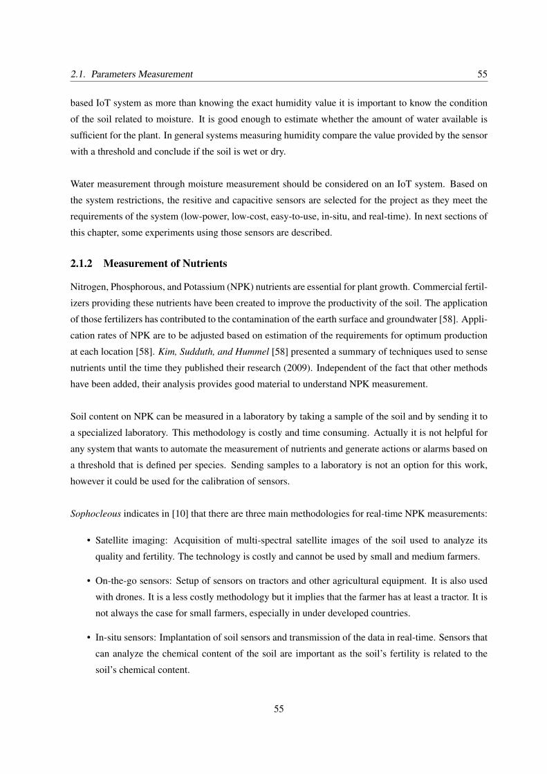
2.1. Parameters Measurement 55
based IoT system as more than knowing the exact humidity value it is important to know the condition
of the soil related to moisture. It is good enough to estimate whether the amount of water available is
sufficient for the plant. In general systems measuring humidity compare the value provided by the sensor
with a threshold and conclude if the soil is wet or dry.
Water measurement through moisture measurement should be considered on an IoT system. Based on
the system restrictions, the resitive and capacitive sensors are selected for the project as they meet the
requirements of the system (low-power, low-cost, easy-to-use, in-situ, and real-time). In next sections of
this chapter, some experiments using those sensors are described.
2.1.2 Measurement of Nutrients
Nitrogen, Phosphorous, and Potassium (NPK) nutrients are essential for plant growth. Commercial fertil-
izers providing these nutrients have been created to improve the productivity of the soil. The application
of those fertilizers has contributed to the contamination of the earth surface and groundwater [58]. Appli-
cation rates of NPK are to be adjusted based on estimation of the requirements for optimum production
at each location [58]. Kim, Sudduth, and Hummel [58] presented a summary of techniques used to sense
nutrients until the time they published their research (2009). Independent of the fact that other methods
have been added, their analysis provides good material to understand NPK measurement.
Soil content on NPK can be measured in a laboratory by taking a sample of the soil and by sending it to
a specialized laboratory. This methodology is costly and time consuming. Actually it is not helpful for
any system that wants to automate the measurement of nutrients and generate actions or alarms based on
a threshold that is defined per species. Sending samples to a laboratory is not an option for this work,
however it could be used for the calibration of sensors.
Sophocleous indicates in [10] that there are three main methodologies for real-time NPK measurements:
• Satellite imaging: Acquisition of multi-spectral satellite images of the soil used to analyze its
quality and fertility. The technology is costly and cannot be used by small and medium farmers.
• On-the-go sensors: Setup of sensors on tractors and other agricultural equipment. It is also used
with drones. It is a less costly methodology but it implies that the farmer has at least a tractor. It is
not always the case for small farmers, especially in under developed countries.
• In-situ sensors: Implantation of soil sensors and transmission of the data in real-time. Sensors that
can analyze the chemical content of the soil are important as the soil’s fertility is related to the
soil’s chemical content.
55
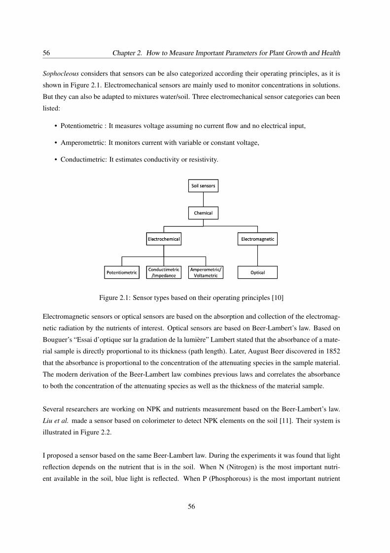
56 Chapter 2. How to Measure Important Parameters for Plant Growth and Health
Sophocleous considers that sensors can be also categorized according their operating principles, as it is
shown in Figure 2.1. Electromechanical sensors are mainly used to monitor concentrations in solutions.
But they can also be adapted to mixtures water/soil. Three electromechanical sensor categories can been
listed:
• Potentiometric : It measures voltage assuming no current flow and no electrical input,
• Amperometrtic: It monitors current with variable or constant voltage,
• Conductimetric: It estimates conductivity or resistivity.
Figure 2.1: Sensor types based on their operating principles [10]
Electromagnetic sensors or optical sensors are based on the absorption and collection of the electromag-
netic radiation by the nutrients of interest. Optical sensors are based on Beer-Lambert’s law. Based on
Bouguer’s “Essai d’optique sur la gradation de la lumière” Lambert stated that the absorbance of a mate-
rial sample is directly proportional to its thickness (path length). Later, August Beer discovered in 1852
that the absorbance is proportional to the concentration of the attenuating species in the sample material.
The modern derivation of the Beer-Lambert law combines previous laws and correlates the absorbance
to both the concentration of the attenuating species as well as the thickness of the material sample.
Several researchers are working on NPK and nutrients measurement based on the Beer-Lambert’s law.
Liu et al. made a sensor based on colorimeter to detect NPK elements on the soil [11]. Their system is
illustrated in Figure 2.2.
I proposed a sensor based on the same Beer-Lambert law. During the experiments it was found that light
reflection depends on the nutrient that is in the soil. When N (Nitrogen) is the most important nutri-
ent available in the soil, blue light is reflected. When P (Phosphorous) is the most important nutrient
56
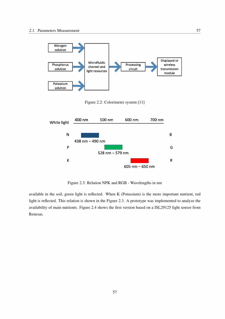
2.1. Parameters Measurement 57
Figure 2.2: Colorimeter system [11]
Figure 2.3: Relation NPK and RGB - Wavelengths in nm
available in the soil, green light is reflected. When K (Potassium) is the more important nutrient, red
light is reflected. This relation is shown in the Figure 2.3. A prototype was implemented to analyze the
availability of main nutrients. Figure 2.4 shows the first version based on a ISL29125 light sensor from
Renesas.
57
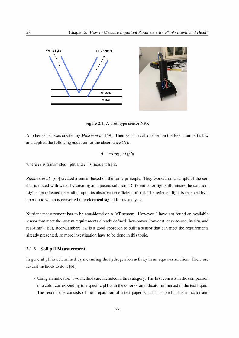
58 Chapter 2. How to Measure Important Parameters for Plant Growth and Health
Figure 2.4: A prototype sensor NPK
Another sensor was created by Masrie et al. [59]. Their sensor is also based on the Beer-Lambert’s law
and applied the following equation for the absorbance (A):
A =−log10 ∗ I1/I0
where I1 is transmitted light and I0 is incident light.
Ramane et al. [60] created a sensor based on the same principle. They worked on a sample of the soil
that is mixed with water by creating an aqueous solution. Different color lights illuminate the solution.
Lights get reflected depending upon its absorbent coefficient of soil. The reflected light is received by a
fiber optic which is converted into electrical signal for its analysis.
Nutrient measurement has to be considered on a IoT system. However, I have not found an available
sensor that meet the system requirements already defined (low-power, low-cost, easy-to-use, in-situ, and
real-time). But, Beer-Lambert law is a good approach to built a sensor that can meet the requirements
already presented, so more investigation have to be done in this topic.
2.1.3 Soil pH Measurement
In general pH is determined by measuring the hydrogen ion activity in an aqueous solution. There are
several methods to do it [61]
• Using an indicator: Two methods are included in this category. The first consists in the comparison
of a color corresponding to a specific pH with the color of an indicator immersed in the test liquid.
The second one consists of the preparation of a test paper which is soaked in the indicator and
58
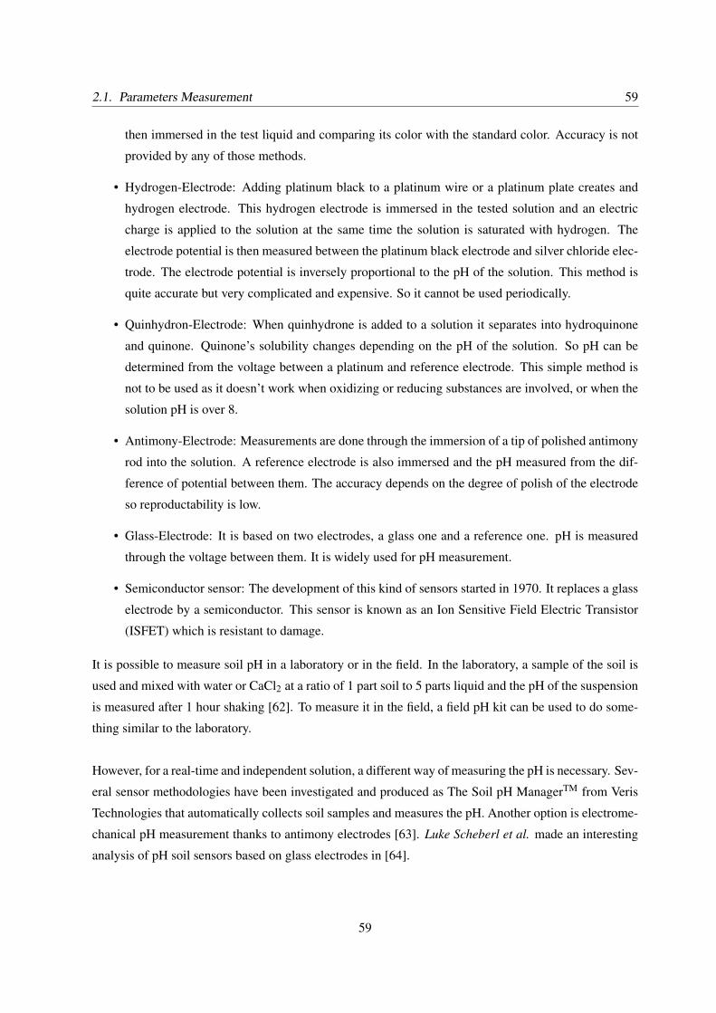
2.1. Parameters Measurement 59
then immersed in the test liquid and comparing its color with the standard color. Accuracy is not
provided by any of those methods.
• Hydrogen-Electrode: Adding platinum black to a platinum wire or a platinum plate creates and
hydrogen electrode. This hydrogen electrode is immersed in the tested solution and an electric
charge is applied to the solution at the same time the solution is saturated with hydrogen. The
electrode potential is then measured between the platinum black electrode and silver chloride elec-
trode. The electrode potential is inversely proportional to the pH of the solution. This method is
quite accurate but very complicated and expensive. So it cannot be used periodically.
• Quinhydron-Electrode: When quinhydrone is added to a solution it separates into hydroquinone
and quinone. Quinone’s solubility changes depending on the pH of the solution. So pH can be
determined from the voltage between a platinum and reference electrode. This simple method is
not to be used as it doesn’t work when oxidizing or reducing substances are involved, or when the
solution pH is over 8.
• Antimony-Electrode: Measurements are done through the immersion of a tip of polished antimony
rod into the solution. A reference electrode is also immersed and the pH measured from the dif-
ference of potential between them. The accuracy depends on the degree of polish of the electrode
so reproductability is low.
• Glass-Electrode: It is based on two electrodes, a glass one and a reference one. pH is measured
through the voltage between them. It is widely used for pH measurement.
• Semiconductor sensor: The development of this kind of sensors started in 1970. It replaces a glass
electrode by a semiconductor. This sensor is known as an Ion Sensitive Field Electric Transistor
(ISFET) which is resistant to damage.
It is possible to measure soil pH in a laboratory or in the field. In the laboratory, a sample of the soil is
used and mixed with water or CaCl2 at a ratio of 1 part soil to 5 parts liquid and the pH of the suspension
is measured after 1 hour shaking [62]. To measure it in the field, a field pH kit can be used to do some-
thing similar to the laboratory.
However, for a real-time and independent solution, a different way of measuring the pH is necessary. Sev-
eral sensor methodologies have been investigated and produced as The Soil pH ManagerTM from Veris
Technologies that automatically collects soil samples and measures the pH. Another option is electrome-
chanical pH measurement thanks to antimony electrodes [63]. Luke Scheberl et al. made an interesting
analysis of pH soil sensors based on glass electrodes in [64].
59
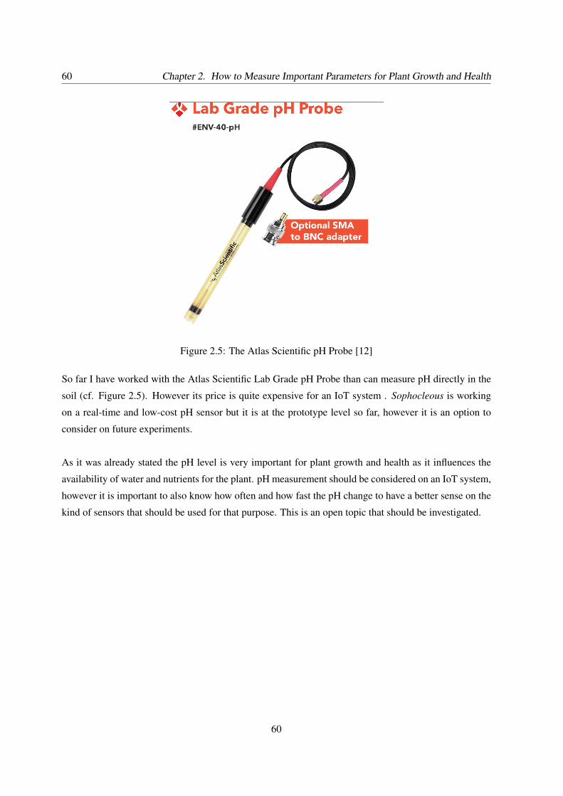
60 Chapter 2. How to Measure Important Parameters for Plant Growth and Health
Figure 2.5: The Atlas Scientific pH Probe [12]
So far I have worked with the Atlas Scientific Lab Grade pH Probe than can measure pH directly in the
soil (cf. Figure 2.5). However its price is quite expensive for an IoT system . Sophocleous is working
on a real-time and low-cost pH sensor but it is at the prototype level so far, however it is an option to
consider on future experiments.
As it was already stated the pH level is very important for plant growth and health as it influences the
availability of water and nutrients for the plant. pH measurement should be considered on an IoT system,
however it is important to also know how often and how fast the pH change to have a better sense on the
kind of sensors that should be used for that purpose. This is an open topic that should be investigated.
60
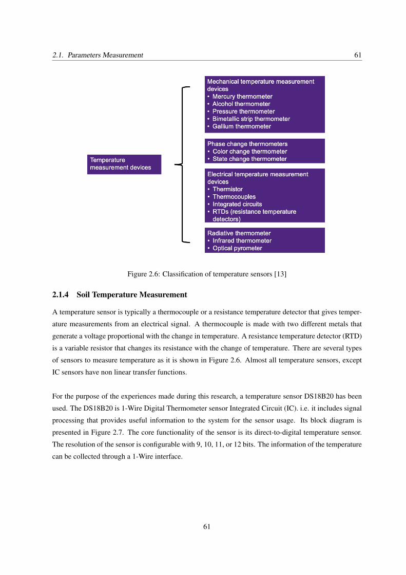
2.1. Parameters Measurement 61
Figure 2.6: Classification of temperature sensors [13]
2.1.4 Soil Temperature Measurement
A temperature sensor is typically a thermocouple or a resistance temperature detector that gives temper-
ature measurements from an electrical signal. A thermocouple is made with two different metals that
generate a voltage proportional with the change in temperature. A resistance temperature detector (RTD)
is a variable resistor that changes its resistance with the change of temperature. There are several types
of sensors to measure temperature as it is shown in Figure 2.6. Almost all temperature sensors, except
IC sensors have non linear transfer functions.
For the purpose of the experiences made during this research, a temperature sensor DS18B20 has been
used. The DS18B20 is 1-Wire Digital Thermometer sensor Integrated Circuit (IC). i.e. it includes signal
processing that provides useful information to the system for the sensor usage. Its block diagram is
presented in Figure 2.7. The core functionality of the sensor is its direct-to-digital temperature sensor.
The resolution of the sensor is configurable with 9, 10, 11, or 12 bits. The information of the temperature
can be collected through a 1-Wire interface.
61
62 Chapter 2. How to Measure Important Parameters for Plant Growth and Health
Figure 2.7: DS18B20 - Simplified block diagram [14]
Soil temperature has to be considered in an IoT system as the one defined as part of this work. Sensors
meeting the system requirements are available and could be used. A temperature sensor, that meet all
restrictions has been selected, DS18B20. It is used in the experiments that are presented in the next
sections of this chapter.
2.1.5 Soil Salinity Measurement
Soil salinity is measured by passing an electric current between two electrodes of a salinity meter. The
electrical conductivity (EC) is affected by the concentration and composition of dissolved salts. As salts
increase the conductivity of a solution, high EC indicates high salinity. The salinity is measured in
deciSiemens per meter (dS/m), or in EC, or in parts per million (ppm). One can note that 1 dS/m is
equivalent to 1.000 EC and to 640 ppm.
Corwin [65] states that five methods have been proposed to determine the soil salinity at field scales:
visual crop observation, electrical conductance of soil solution extracts, in situ measurement of electrical
resistivity, non invasive measurement of electrical conductance, and in-situ measurement of electrical
conductance .
The methods mentioned above are quite expensive and not suitable for a low-cost and low-power IoT
system. A more suitable method to measure the soil salinity is through electrical conductivity sensors,
such as the TEROS-12 which can also measure other parameters as soil volumetric water content and
temperature. Others available sensors are the PS-2195 from PASCO and 5000L from ENVCO. Roux
presented a capacitive sensor that could be used for real-time systems [66]. All those sensors are still
62
2.1. Parameters Measurement 63
quite expensive, so their usage in an IoT system with the requirements already stated (low-power, low-
cost, easy-to-use, in-situ, and real-time) is not possible.
Soil salinity is an important parameter that should be measured. However the cost of a sensor to be able
to get the salinity value in an IoT system is still too high. So more researches have to be done in this
domain to find or build a low-cost and low-power EC sensor to get the salinity value in real-time. As for
the pH, it is important to know what makes salinity to change and how often and how fast it can change.
2.1.6 The Light
Outdoor plantations are exposed to sun light composed by all necessary wavelengths. Its measurement
provides information regarding the quality and quantity of the light. No direct action can be taken. Indoor
plantations are exposed to artificial light. Its measurement is more accurate and can lead to automatic
actions to ensure an efficient production. Only ultraviolet, blue, red, and far red are required. Thus,
specific LEDs to measure the intensity of those colors (wavelengths) are proposed for the IoT system.
There are several sensors to measure the intensity of the light, such as photodiodes and phototransistors
of each color in the light. It is possible t mention the ISL2915 [67] and the GY-302 BH1750 [68].
Light measurement could be considered in an IoT system when working in greenhouses.
2.1.7 The Weather
Weather station data can be used by in an IoT system. The system can capture data from weather stations
through Internet and analyze it to generate the corresponding alarms to the farmer. Information coming
from weather stations can also be useful to define the best moment to irrigate as high temperatures and
fast winds influence the evotranspiration.
Weather information is considered in the presented IoT system as an input of the system.
2.1.8 Summary
Table 2.1 presents the different parameters associated with their measurement methodology, the selected
sensor and how they meet the requirements defined at the beginning of the chapter
It can be noted that despite the fact that there are several methodologies to measure the parameters that
have been defined, very few sensors that meet all the requirements of the system are available. Conse-
quently, it limits the effectiveness of the system under design. As several sensors that could meet the
requirements are under development, the designed system has to be flexible. Indeed additional sensors
should be added in the future.
63
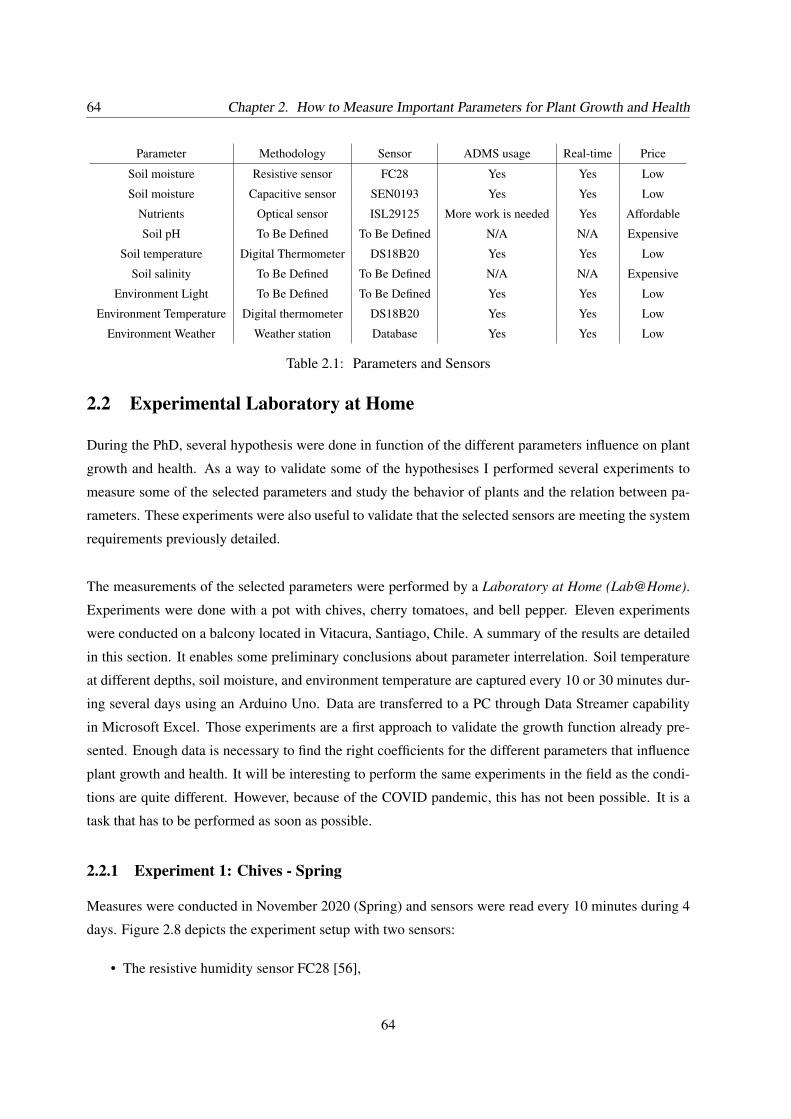
64 Chapter 2. How to Measure Important Parameters for Plant Growth and Health
Parameter Methodology Sensor ADMS usage Real-time Price
Soil moisture Resistive sensor FC28 Yes Yes Low
Soil moisture Capacitive sensor SEN0193 Yes Yes Low
Nutrients Optical sensor ISL29125 More work is needed Yes Affordable
Soil pH To Be Defined To Be Defined N/A N/A Expensive
Soil temperature Digital Thermometer DS18B20 Yes Yes Low
Soil salinity To Be Defined To Be Defined N/A N/A Expensive
Environment Light To Be Defined To Be Defined Yes Yes Low
Environment Temperature Digital thermometer DS18B20 Yes Yes Low
Environment Weather Weather station Database Yes Yes Low
Table 2.1: Parameters and Sensors
2.2 Experimental Laboratory at Home
During the PhD, several hypothesis were done in function of the different parameters influence on plant
growth and health. As a way to validate some of the hypothesises I performed several experiments to
measure some of the selected parameters and study the behavior of plants and the relation between pa-
rameters. These experiments were also useful to validate that the selected sensors are meeting the system
requirements previously detailed.
The measurements of the selected parameters were performed by a Laboratory at Home (Lab@Home).
Experiments were done with a pot with chives, cherry tomatoes, and bell pepper. Eleven experiments
were conducted on a balcony located in Vitacura, Santiago, Chile. A summary of the results are detailed
in this section. It enables some preliminary conclusions about parameter interrelation. Soil temperature
at different depths, soil moisture, and environment temperature are captured every 10 or 30 minutes dur-
ing several days using an Arduino Uno. Data are transferred to a PC through Data Streamer capability
in Microsoft Excel. Those experiments are a first approach to validate the growth function already pre-
sented. Enough data is necessary to find the right coefficients for the different parameters that influence
plant growth and health. It will be interesting to perform the same experiments in the field as the condi-
tions are quite different. However, because of the COVID pandemic, this has not been possible. It is a
task that has to be performed as soon as possible.
2.2.1 Experiment 1: Chives - Spring
Measures were conducted in November 2020 (Spring) and sensors were read every 10 minutes during 4
days. Figure 2.8 depicts the experiment setup with two sensors:
• The resistive humidity sensor FC28 [56],
64
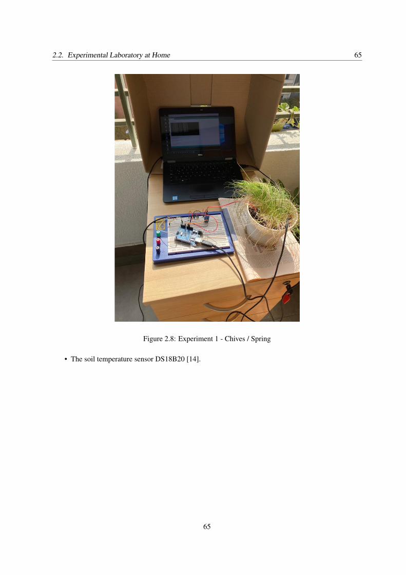
2.2. Experimental Laboratory at Home 65
Figure 2.8: Experiment 1 - Chives / Spring
• The soil temperature sensor DS18B20 [14].
65
66 Chapter 2. How to Measure Important Parameters for Plant Growth and Health
Moisture have small changes during 2 days and rapidly move to a different situation and will remain
there as it is shown in Figure 2.9. Soil was irrigated at the beginning of the experiment. From there the
plant started to absorb water based on the specific species needs. After a couple of days in which the
sensor delivered different values within the wet zone, the sensor provided a value indicating that the soil
was dry. Once the dry situation was confirmed by several measurements, the plant was irrigated.
Figure 2.9: Soil temperature and soil moisture over time
It is important to remember that the quantity of water that the plant is absorbing is not measured. Ac-
tually, the measurement is done on the humidity of the soil. Plant’s thirst is measured indirectly. Soil
temperature follows a typical wave for a Mediterranean climate such as Santiago climate. Soil Tem-
perature (ST) is following a sine wave over time. So it could be represented as ST = x ∗ sinz where z
66
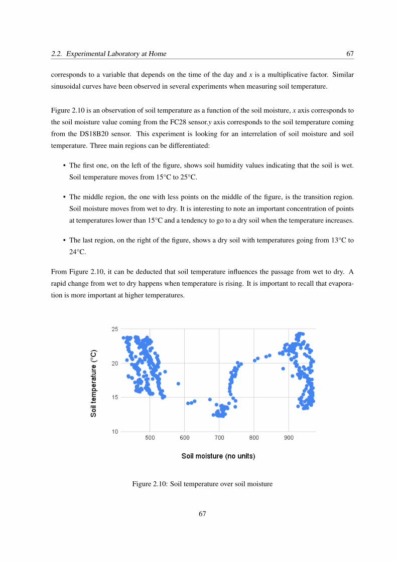
2.2. Experimental Laboratory at Home 67
corresponds to a variable that depends on the time of the day and x is a multiplicative factor. Similar
sinusoidal curves have been observed in several experiments when measuring soil temperature.
Figure 2.10 is an observation of soil temperature as a function of the soil moisture, x axis corresponds to
the soil moisture value coming from the FC28 sensor.y axis corresponds to the soil temperature coming
from the DS18B20 sensor. This experiment is looking for an interrelation of soil moisture and soil
temperature. Three main regions can be differentiated:
• The first one, on the left of the figure, shows soil humidity values indicating that the soil is wet.
Soil temperature moves from 15°C to 25°C.
• The middle region, the one with less points on the middle of the figure, is the transition region.
Soil moisture moves from wet to dry. It is interesting to note an important concentration of points
at temperatures lower than 15°C and a tendency to go to a dry soil when the temperature increases.
• The last region, on the right of the figure, shows a dry soil with temperatures going from 13°C to
24°C.
From Figure 2.10, it can be deducted that soil temperature influences the passage from wet to dry. A
rapid change from wet to dry happens when temperature is rising. It is important to recall that evapora-
tion is more important at higher temperatures.
Figure 2.10: Soil temperature over soil moisture
67
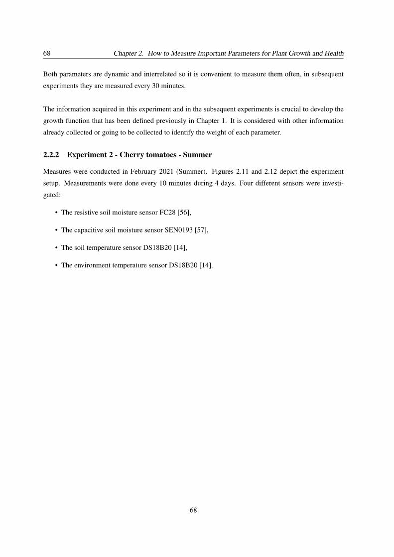
68 Chapter 2. How to Measure Important Parameters for Plant Growth and Health
Both parameters are dynamic and interrelated so it is convenient to measure them often, in subsequent
experiments they are measured every 30 minutes.
The information acquired in this experiment and in the subsequent experiments is crucial to develop the
growth function that has been defined previously in Chapter 1. It is considered with other information
already collected or going to be collected to identify the weight of each parameter.
2.2.2 Experiment 2 - Cherry tomatoes - Summer
Measures were conducted in February 2021 (Summer). Figures 2.11 and 2.12 depict the experiment
setup. Measurements were done every 10 minutes during 4 days. Four different sensors were investi-
gated:
• The resistive soil moisture sensor FC28 [56],
• The capacitive soil moisture sensor SEN0193 [57],
• The soil temperature sensor DS18B20 [14],
• The environment temperature sensor DS18B20 [14].
68
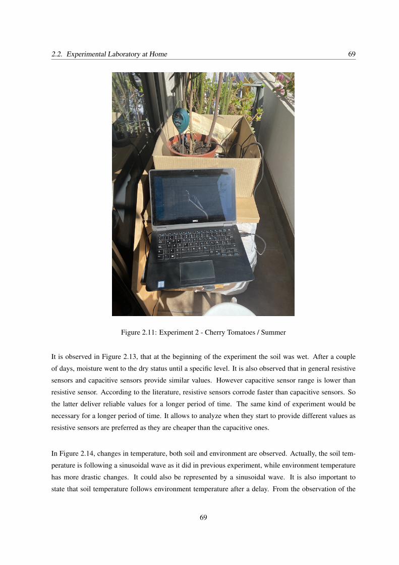
2.2. Experimental Laboratory at Home 69
Figure 2.11: Experiment 2 - Cherry Tomatoes / Summer
It is observed in Figure 2.13, that at the beginning of the experiment the soil was wet. After a couple
of days, moisture went to the dry status until a specific level. It is also observed that in general resistive
sensors and capacitive sensors provide similar values. However capacitive sensor range is lower than
resistive sensor. According to the literature, resistive sensors corrode faster than capacitive sensors. So
the latter deliver reliable values for a longer period of time. The same kind of experiment would be
necessary for a longer period of time. It allows to analyze when they start to provide different values as
resistive sensors are preferred as they are cheaper than the capacitive ones.
In Figure 2.14, changes in temperature, both soil and environment are observed. Actually, the soil tem-
perature is following a sinusoidal wave as it did in previous experiment, while environment temperature
has more drastic changes. It could also be represented by a sinusoidal wave. It is also important to
state that soil temperature follows environment temperature after a delay. From the observation of the
69
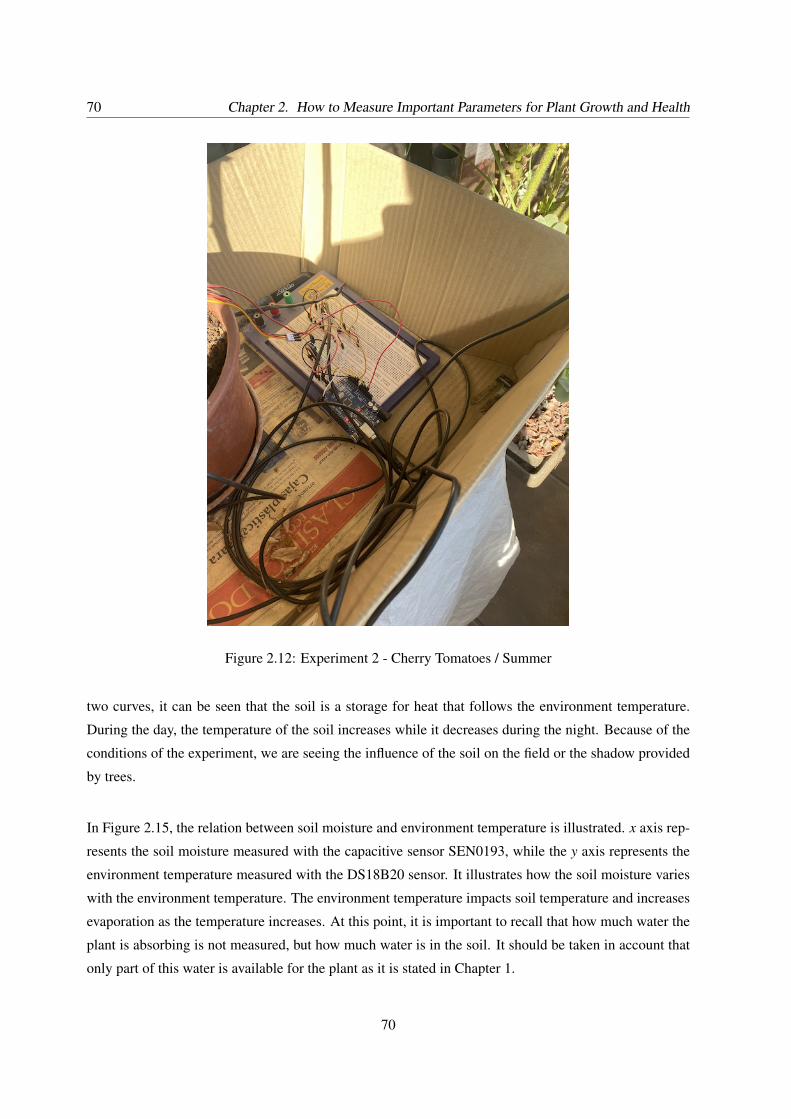
70 Chapter 2. How to Measure Important Parameters for Plant Growth and Health
Figure 2.12: Experiment 2 - Cherry Tomatoes / Summer
two curves, it can be seen that the soil is a storage for heat that follows the environment temperature.
During the day, the temperature of the soil increases while it decreases during the night. Because of the
conditions of the experiment, we are seeing the influence of the soil on the field or the shadow provided
by trees.
In Figure 2.15, the relation between soil moisture and environment temperature is illustrated. x axis rep-
resents the soil moisture measured with the capacitive sensor SEN0193, while the y axis represents the
environment temperature measured with the DS18B20 sensor. It illustrates how the soil moisture varies
with the environment temperature. The environment temperature impacts soil temperature and increases
evaporation as the temperature increases. At this point, it is important to recall that how much water the
plant is absorbing is not measured, but how much water is in the soil. It should be taken in account that
only part of this water is available for the plant as it is stated in Chapter 1.
70
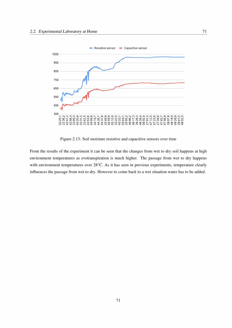
2.2. Experimental Laboratory at Home 71
Figure 2.13: Soil moisture resistive and capacitive sensors over time
From the results of the experiment it can be seen that the changes from wet to dry soil happens at high
environment temperatures as evotranspiration is much higher. The passage from wet to dry happens
with environment temperatures over 28°C. As it has seen in previous experiments, temperature clearly
influences the passage from wet to dry. However to come back to a wet situation water has to be added.
71
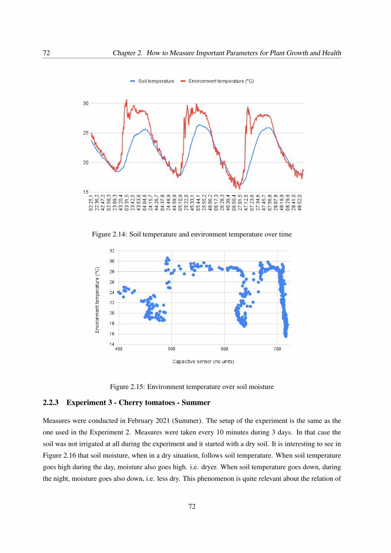
72 Chapter 2. How to Measure Important Parameters for Plant Growth and Health
Figure 2.14: Soil temperature and environment temperature over time
Figure 2.15: Environment temperature over soil moisture
2.2.3 Experiment 3 - Cherry tomatoes - Summer
Measures were conducted in February 2021 (Summer). The setup of the experiment is the same as the
one used in the Experiment 2. Measures were taken every 10 minutes during 3 days. In that case the
soil was not irrigated at all during the experiment and it started with a dry soil. It is interesting to see in
Figure 2.16 that soil moisture, when in a dry situation, follows soil temperature. When soil temperature
goes high during the day, moisture also goes high. i.e. dryer. When soil temperature goes down, during
the night, moisture goes also down, i.e. less dry. This phenomenon is quite relevant about the relation of
72
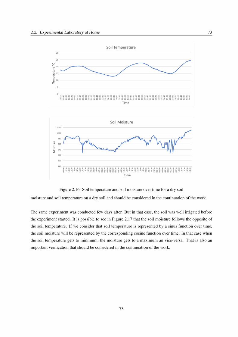
2.2. Experimental Laboratory at Home 73
Figure 2.16: Soil temperature and soil moisture over time for a dry soil
moisture and soil temperature on a dry soil and should be considered in the continuation of the work.
The same experiment was conducted few days after. But in that case, the soil was well irrigated before
the experiment started. It is possible to see in Figure 2.17 that the soil moisture follows the opposite of
the soil temperature. If we consider that soil temperature is represented by a sinus function over time,
the soil moisture will be represented by the corresponding cosine function over time. In that case when
the soil temperature gets to minimum, the moisture gets to a maximum an vice-versa. That is also an
important verification that should be considered in the continuation of the work.
73
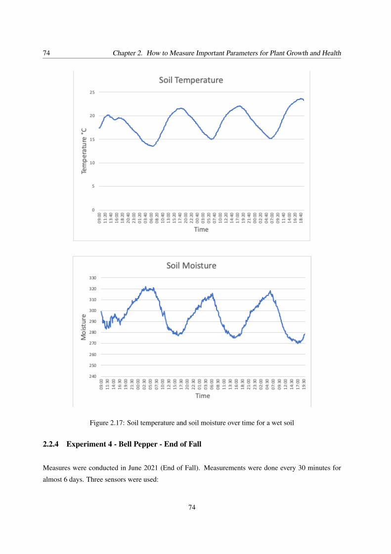
74 Chapter 2. How to Measure Important Parameters for Plant Growth and Health
Figure 2.17: Soil temperature and soil moisture over time for a wet soil
2.2.4 Experiment 4 - Bell Pepper - End of Fall
Measures were conducted in June 2021 (End of Fall). Measurements were done every 30 minutes for
almost 6 days. Three sensors were used:
74
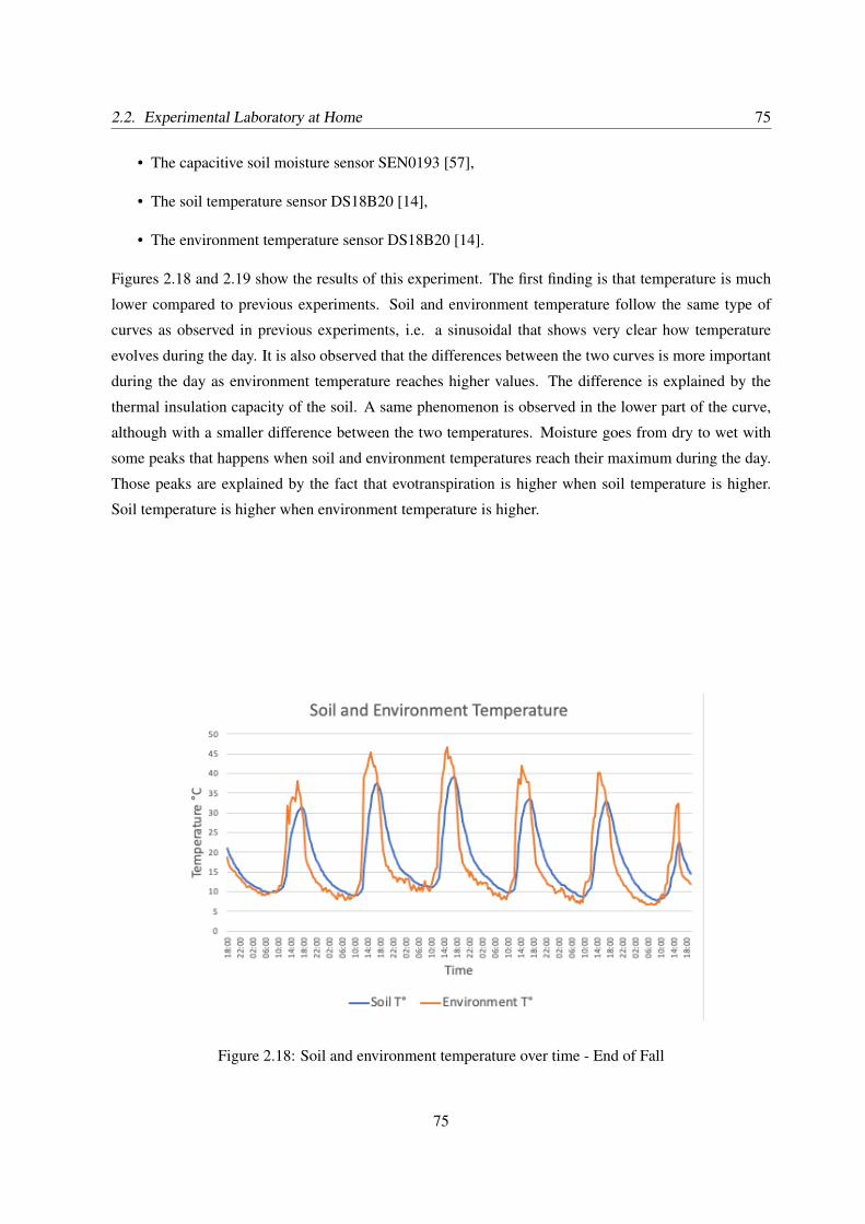
2.2. Experimental Laboratory at Home 75
• The capacitive soil moisture sensor SEN0193 [57],
• The soil temperature sensor DS18B20 [14],
• The environment temperature sensor DS18B20 [14].
Figures 2.18 and 2.19 show the results of this experiment. The first finding is that temperature is much
lower compared to previous experiments. Soil and environment temperature follow the same type of
curves as observed in previous experiments, i.e. a sinusoidal that shows very clear how temperature
evolves during the day. It is also observed that the differences between the two curves is more important
during the day as environment temperature reaches higher values. The difference is explained by the
thermal insulation capacity of the soil. A same phenomenon is observed in the lower part of the curve,
although with a smaller difference between the two temperatures. Moisture goes from dry to wet with
some peaks that happens when soil and environment temperatures reach their maximum during the day.
Those peaks are explained by the fact that evotranspiration is higher when soil temperature is higher.
Soil temperature is higher when environment temperature is higher.
Figure 2.18: Soil and environment temperature over time - End of Fall
75
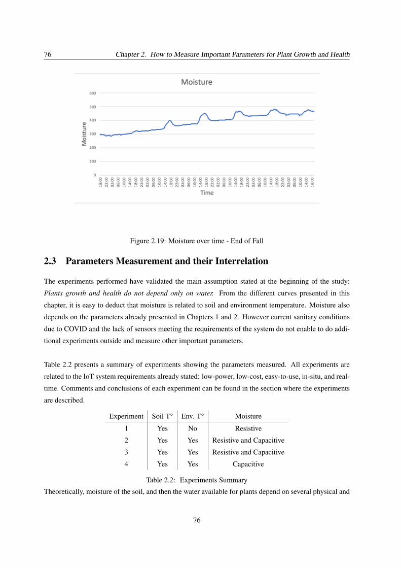
76 Chapter 2. How to Measure Important Parameters for Plant Growth and Health
Figure 2.19: Moisture over time - End of Fall
2.3 Parameters Measurement and their Interrelation
The experiments performed have validated the main assumption stated at the beginning of the study:
Plants growth and health do not depend only on water. From the different curves presented in this
chapter, it is easy to deduct that moisture is related to soil and environment temperature. Moisture also
depends on the parameters already presented in Chapters 1 and 2. However current sanitary conditions
due to COVID and the lack of sensors meeting the requirements of the system do not enable to do addi-
tional experiments outside and measure other important parameters.
Table 2.2 presents a summary of experiments showing the parameters measured. All experiments are
related to the IoT system requirements already stated: low-power, low-cost, easy-to-use, in-situ, and real-
time. Comments and conclusions of each experiment can be found in the section where the experiments
are described.
Experiment Soil T° Env. T° Moisture
1 Yes No Resistive
2 Yes Yes Resistive and Capacitive
3 Yes Yes Resistive and Capacitive
4 Yes Yes Capacitive
Table 2.2: Experiments Summary
Theoretically, moisture of the soil, and then the water available for plants depend on several physical and
76
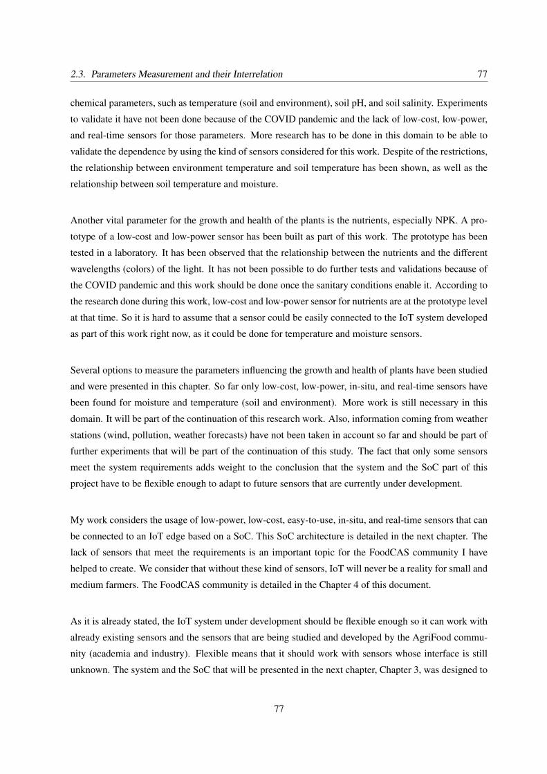
2.3. Parameters Measurement and their Interrelation 77
chemical parameters, such as temperature (soil and environment), soil pH, and soil salinity. Experiments
to validate it have not been done because of the COVID pandemic and the lack of low-cost, low-power,
and real-time sensors for those parameters. More research has to be done in this domain to be able to
validate the dependence by using the kind of sensors considered for this work. Despite of the restrictions,
the relationship between environment temperature and soil temperature has been shown, as well as the
relationship between soil temperature and moisture.
Another vital parameter for the growth and health of the plants is the nutrients, especially NPK. A pro-
totype of a low-cost and low-power sensor has been built as part of this work. The prototype has been
tested in a laboratory. It has been observed that the relationship between the nutrients and the different
wavelengths (colors) of the light. It has not been possible to do further tests and validations because of
the COVID pandemic and this work should be done once the sanitary conditions enable it. According to
the research done during this work, low-cost and low-power sensor for nutrients are at the prototype level
at that time. So it is hard to assume that a sensor could be easily connected to the IoT system developed
as part of this work right now, as it could be done for temperature and moisture sensors.
Several options to measure the parameters influencing the growth and health of plants have been studied
and were presented in this chapter. So far only low-cost, low-power, in-situ, and real-time sensors have
been found for moisture and temperature (soil and environment). More work is still necessary in this
domain. It will be part of the continuation of this research work. Also, information coming from weather
stations (wind, pollution, weather forecasts) have not been taken in account so far and should be part of
further experiments that will be part of the continuation of this study. The fact that only some sensors
meet the system requirements adds weight to the conclusion that the system and the SoC part of this
project have to be flexible enough to adapt to future sensors that are currently under development.
My work considers the usage of low-power, low-cost, easy-to-use, in-situ, and real-time sensors that can
be connected to an IoT edge based on a SoC. This SoC architecture is detailed in the next chapter. The
lack of sensors that meet the requirements is an important topic for the FoodCAS community I have
helped to create. We consider that without these kind of sensors, IoT will never be a reality for small and
medium farmers. The FoodCAS community is detailed in the Chapter 4 of this document.
As it is already stated, the IoT system under development should be flexible enough so it can work with
already existing sensors and the sensors that are being studied and developed by the AgriFood commu-
nity (academia and industry). Flexible means that it should work with sensors whose interface is still
unknown. The system and the SoC that will be presented in the next chapter, Chapter 3, was designed to
77
78 Chapter 2. How to Measure Important Parameters for Plant Growth and Health
have different interfaces so it can accept new sensors.
All these constraints reemphasize the main statement of this project, smart agriculture for small and
medium farmers cannot be done with existing systems and sensors as it is quite expensive and consumes
a lot of power. Also the communication ways those systems have do not meet the requirement of low-
cost or are unavailable in rural areas. In the next chapter, an IoT system designed for the purpose of IoT
systems for smart agriculture considering especially small to medium farmers is presented. This system
is composed by a SoC (system on a chip) containing a 32 bits processor able to do edge computing,
instructions and data memories, and several peripherals I/Os for the connection of existing sensors and
sensors under development. The system also considers a LoRa interface that provides low-cost commu-
nication with the cloud through a LoRa gateway. The amount of data to be transmitted justifies the usage
of LPWAN systems, among them LoRa has been selected because it is low-power and low-cost. LoRa is
also easy to deploy in the field so it meets the requirements stated for the IoT system implement during
this study.
78
CHAPTER
3A DEDICATED SOC FOR
SMART AGRICULTURE
Sommaire3.1 The IoT System and the SoC . . . . . . . . . . . . . . . . . . . . . . . . . . . . . . 80
3.1.1 Main Architecture of the System . . . . . . . . . . . . . . . . . . . . . . . . . 82
3.1.2 Proof of Concept . . . . . . . . . . . . . . . . . . . . . . . . . . . . . . . . . 84
3.1.3 SoC Architecture . . . . . . . . . . . . . . . . . . . . . . . . . . . . . . . . . 86
3.2 SoC Design Flow . . . . . . . . . . . . . . . . . . . . . . . . . . . . . . . . . . . . . 90
3.2.1 Register Transfer Level (RTL) Generation . . . . . . . . . . . . . . . . . . . . 91
3.2.2 FPGA Implementation Option . . . . . . . . . . . . . . . . . . . . . . . . . . 92
3.2.3 ASIC Implementation Option . . . . . . . . . . . . . . . . . . . . . . . . . . 93
3.3 IP Usage . . . . . . . . . . . . . . . . . . . . . . . . . . . . . . . . . . . . . . . . . 97
3.3.1 The processor . . . . . . . . . . . . . . . . . . . . . . . . . . . . . . . . . . . 97
3.3.2 Memories . . . . . . . . . . . . . . . . . . . . . . . . . . . . . . . . . . . . . 97
3.3.3 I/O Peripherals . . . . . . . . . . . . . . . . . . . . . . . . . . . . . . . . . . 97
3.4 SoC and System Power Analysis . . . . . . . . . . . . . . . . . . . . . . . . . . . . 98
3.5 Connecting the SoC to the Outside World . . . . . . . . . . . . . . . . . . . . . . 99
79
80 Chapter 3. A Dedicated SoC for Smart Agriculture
The main parameters that affect plants growth and health have been presented, detailing their impact
on productivity. Some of the presented parameters where chosen to be part of the system that was
designed. The measurement technologies and the available sensors were presented having in mind the
requirements of the system: low-power, low-cost, easy-to-use, in-situ, and real-time. Some experiments
using soil temperature as well as soil moisture were also detailed. They provide some interesting insights
and ideas about parameter interrelation It has also been shown that sensors for some parameters that
are compliant with the proposed requirements exist only at the prototype level, so additional research is
still necessary in this domain. In this chapter, the IoT system, especially the designed SoC, are presented.
Some specifications and justification are provided for the different components that are part of the system
and the SoC. The system design flow and the SoC design flow are also presented in details. The used
IP in the SoC is detailed as well as the main results of the SoC, Performance, Power and Area (PPA) at
different levels of the design flow.
3.1 The IoT System and the SoC
It has been stated in the previous chapters that an IoT system for agriculture considering small and
medium farmers must have at least the following characteristics:
• Low-power as the device has to work for at least 3 years far from any power supply,
• Able to process data at the edge as communications are not always available in the rural areas, and
even if they are, their cost can be prohibitive,
• Low-cost as small and medium farmers do not have the possibility to invest in technology,
• Easy-to-use as the target users do not have digital skills.
After a deep analysis of the requirements and the state of the art of precision and smart agriculture, I have
concluded that the system should act as a smart edge and be able to process the data through according
to the edge computing principles [35]. So, the edge is composed by a SoC capturing data from sensors,
analyzing it, and taking the corresponding actions that could be a direct action on the crops such as ir-
rigation or fertilization, or a message to the farmer. The system should also be able to send data to the
80
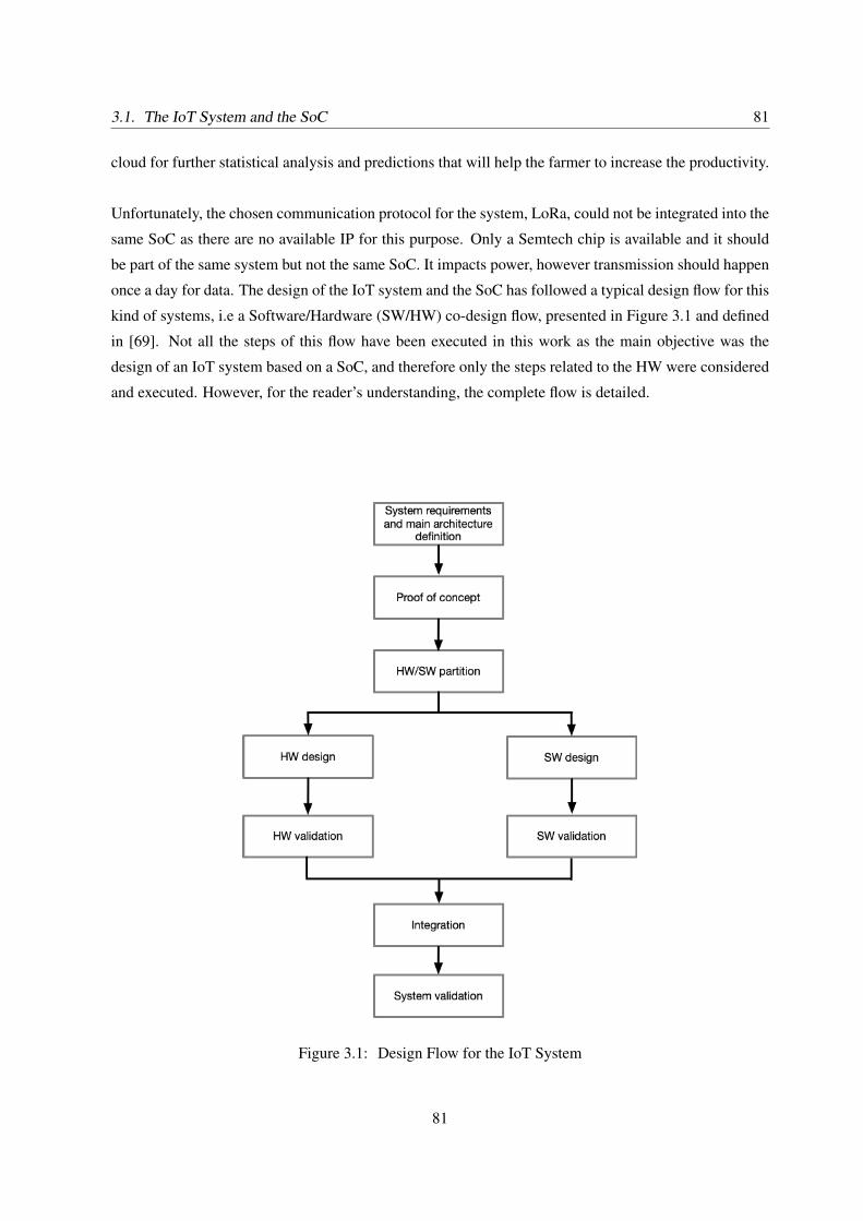
3.1. The IoT System and the SoC 81
cloud for further statistical analysis and predictions that will help the farmer to increase the productivity.
Unfortunately, the chosen communication protocol for the system, LoRa, could not be integrated into the
same SoC as there are no available IP for this purpose. Only a Semtech chip is available and it should
be part of the same system but not the same SoC. It impacts power, however transmission should happen
once a day for data. The design of the IoT system and the SoC has followed a typical design flow for this
kind of systems, i.e a Software/Hardware (SW/HW) co-design flow, presented in Figure 3.1 and defined
in [69]. Not all the steps of this flow have been executed in this work as the main objective was the
design of an IoT system based on a SoC, and therefore only the steps related to the HW were considered
and executed. However, for the reader’s understanding, the complete flow is detailed.
Figure 3.1: Design Flow for the IoT System
81
82 Chapter 3. A Dedicated SoC for Smart Agriculture
• System requirements and main architecture features: The requirements of the system, e.g. an
IoT smart agriculture system, are defined and agreed with the potential users of the system, in that
case the small and medium farmers. It is very important at that step to listen the potential users as
they have a lot of knowledge that should be used by the system under design. During this step the
main architecture of the system is drafted.
• Proof of concept: A first version of the system is generated from a development platform. The
purpose of this step is to validate that the requirements of the system can be reached. In the case
of this work a Synopsys DesignWare ARC EM Starter Kit [70] was selected.
• HW/SW partition: The design team has decided which parts of the system will be implemented
in HW and which parts in SW. Once the partition is defined, the work is separated in two parts,
one related to the HW design, and the other one to the SW design. In general, two different
teams design separately these two parts. For the work of this thesis, an SoC including a proces-
sor, Instruction Closely Coupled Memory (ICCM), Data Closely Coupled Memory (DCCM), and
peripheral I/Os will be designed as HW of the system. The SW of the system should include the
drivers for the peripheral I/Os. For the purpose of this document, only the HW design, specifically
the SoC design will be detailed.
• HW design: All the HW of the system is designed. For this work, the design of the SoC was
completed.
• HW validation: The designed HW is validated against the requirements of the system that have
to be reached through the HW.
• SW design: The SW defined for the system is developed. This step is not part of this work. Only
some programs were developed during the proof of concept step and other routines to validate the
SoC.
• SW validation: Several tests and regressions test are executed to validate the SW of the system
and checking its compliance with the requirements.
• Integration: HW and SW are integrated conforming a system that meets the defined requirements.
• System validation: The whole system is validated running the test cases used to validate the
SW and some additional ones that are created during the development of the SW and during the
integration HW/SW. The regression tests are also applied to validate the system.
3.1.1 Main Architecture of the System
The main architecture of the IoT edge is presented in Figure 3.2. The edge has at least five main parts:
82
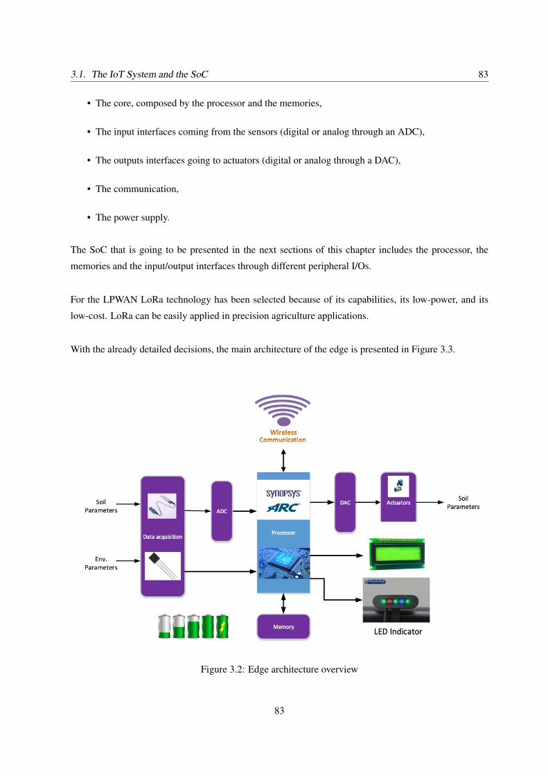
3.1. The IoT System and the SoC 83
• The core, composed by the processor and the memories,
• The input interfaces coming from the sensors (digital or analog through an ADC),
• The outputs interfaces going to actuators (digital or analog through a DAC),
• The communication,
• The power supply.
The SoC that is going to be presented in the next sections of this chapter includes the processor, the
memories and the input/output interfaces through different peripheral I/Os.
For the LPWAN LoRa technology has been selected because of its capabilities, its low-power, and its
low-cost. LoRa can be easily applied in precision agriculture applications.
With the already detailed decisions, the main architecture of the edge is presented in Figure 3.3.
Figure 3.2: Edge architecture overview
83
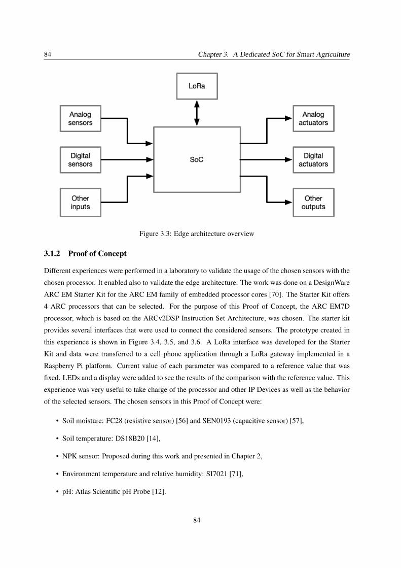
84 Chapter 3. A Dedicated SoC for Smart Agriculture
Figure 3.3: Edge architecture overview
3.1.2 Proof of Concept
Different experiences were performed in a laboratory to validate the usage of the chosen sensors with the
chosen processor. It enabled also to validate the edge architecture. The work was done on a DesignWare
ARC EM Starter Kit for the ARC EM family of embedded processor cores [70]. The Starter Kit offers
4 ARC processors that can be selected. For the purpose of this Proof of Concept, the ARC EM7D
processor, which is based on the ARCv2DSP Instruction Set Architecture, was chosen. The starter kit
provides several interfaces that were used to connect the considered sensors. The prototype created in
this experience is shown in Figure 3.4, 3.5, and 3.6. A LoRa interface was developed for the Starter
Kit and data were transferred to a cell phone application through a LoRa gateway implemented in a
Raspberry Pi platform. Current value of each parameter was compared to a reference value that was
fixed. LEDs and a display were added to see the results of the comparison with the reference value. This
experience was very useful to take charge of the processor and other IP Devices as well as the behavior
of the selected sensors. The chosen sensors in this Proof of Concept were:
• Soil moisture: FC28 (resistive sensor) [56] and SEN0193 (capacitive sensor) [57],
• Soil temperature: DS18B20 [14],
• NPK sensor: Proposed during this work and presented in Chapter 2,
• Environment temperature and relative humidity: SI7021 [71],
• pH: Atlas Scientific pH Probe [12].
84
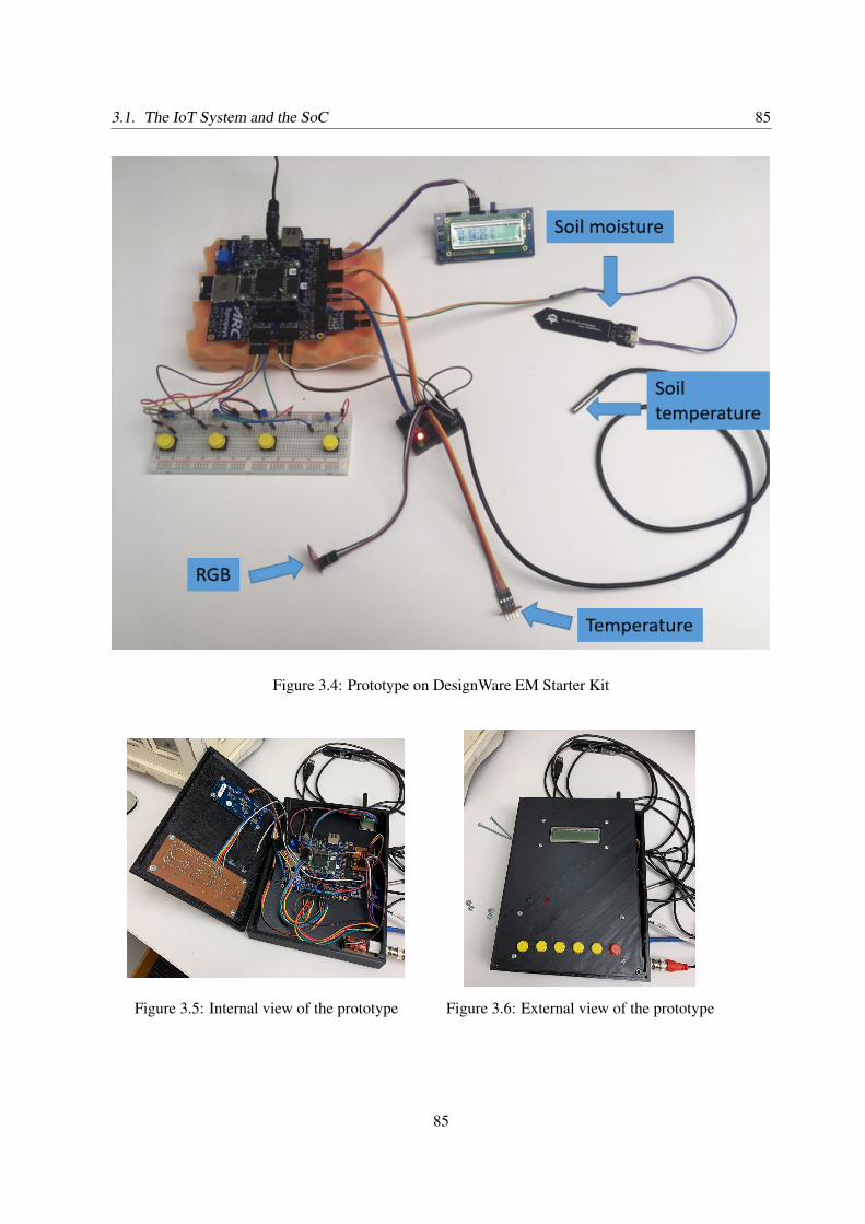
3.1. The IoT System and the SoC 85
Figure 3.4: Prototype on DesignWare EM Starter Kit
Figure 3.5: Internal view of the prototype Figure 3.6: External view of the prototype
85
86 Chapter 3. A Dedicated SoC for Smart Agriculture
All defined objectives were met during this experiment. The Proof of Concept considered the usage
of buttons to select the parameter to be measured, a display to show the measured values, and LEDs
indicating if the measured value was over a threshold for the specific parameter: red means over the
threshold and green means below the threshold. For each parameter, a driver for the corresponding
connection with the platform was selected and implemented (I2C, SPI, 1-wire, etc.).
3.1.3 SoC Architecture
As presented in Chapter 1, the majority of existing systems uses an out of the shelf platform and only
measure soil moisture and soil temperature. They are usually built around a standard and universal elec-
tronic device, platform, or processor that is not necessarily designed with respect to the application as
they are not optimized in terms of system cost and power consumption. Based on the research I have
focused on IoT systems for small and medium farmers, I propose an approach where cost and power are
the main requirements and taking also in considerations additional parameters such as soil salinity, soil
pH, nutrients, etc. To achieve all those requirements, a SoC has been designed as part of this work. The
SoC should also be able to store data for at least 2 days to prevent connectivity issues.
Smart Agriculture, implies the capture of some parameters through sensors and the incorporation of ad-
ditional data, such as weather or soil texture, the process of the captured values in the edge, the activation
of actuators, and the transmission of the data for information and for further analysis. So, the SoC should
contain at least a processor, an ICCM, a DCCM, and some I/O peripherals. The choice of I/O peripherals
is an additional design challenge, as more peripherals involves more area and larger power consumption.
However, it is important to keep the flexibility of the system. For that reason, it has been decided to
restrict 2 peripheral per type, except for I2C and SPI, where only one master peripheral was included.
Designers of systems using this SoC will have to pay attention to power and optimize it through the se-
lection of sensors and the SW development. It will also be convenient to have the communication system
inside the SoC. However for the selected communication technology, an external component will be used.
The general architecture of the designed SoC is detailed in Figure 3.7. One can see the core of the
processor considering a three steps pipeline (fetch, execute, and commit), an ICCM, a DCCM, and the
required Interrupt Controller and the System Control. 12 I/O peripherals have been added to the SoC.
They are described later in the chapter. The selection of the quantity and type of I/O answer the flexibility
requirement argued in Chapter 2. It is quite difficult to define what could be used in the future. So, a
trade-off between flexibility, area, and power consumption has been made.
Two memories have been allocated. One for the ICCM and another one for the DCCM. These memories
86
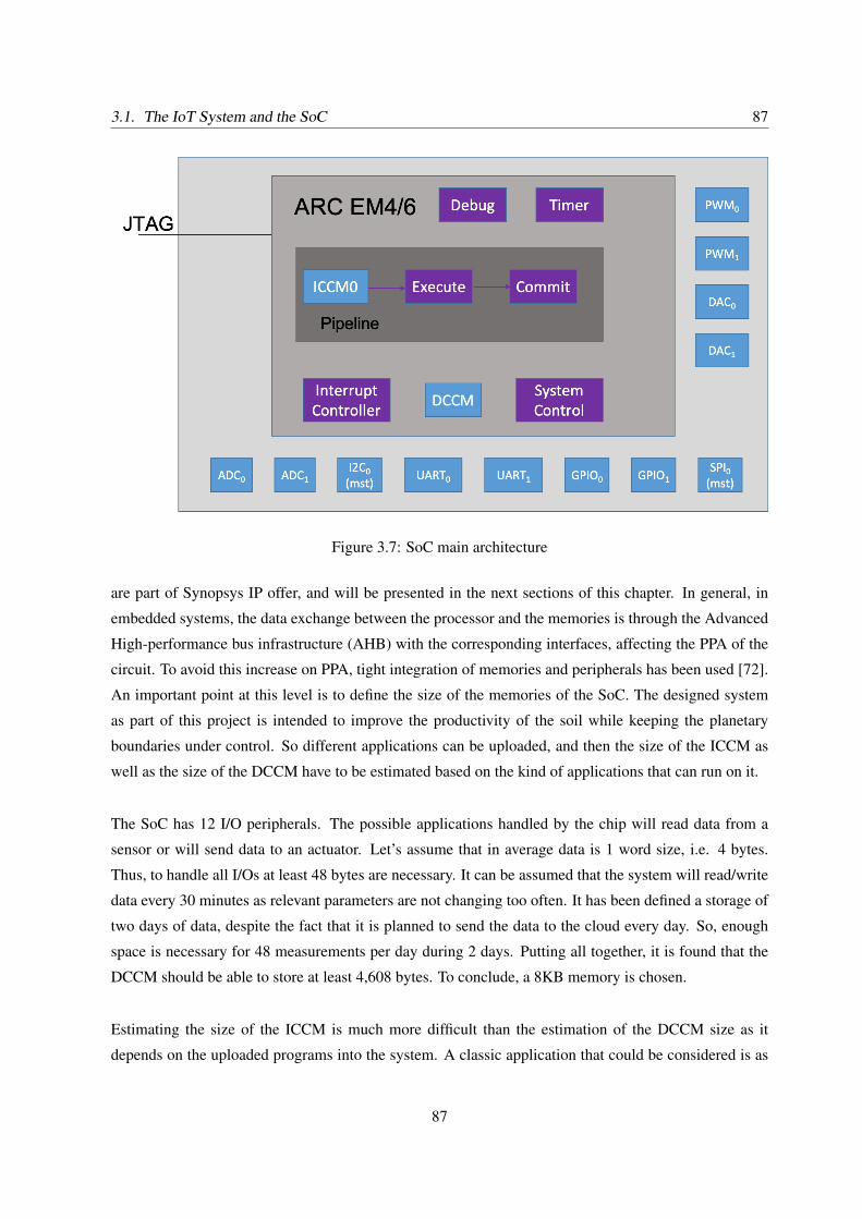
3.1. The IoT System and the SoC 87
Figure 3.7: SoC main architecture
are part of Synopsys IP offer, and will be presented in the next sections of this chapter. In general, in
embedded systems, the data exchange between the processor and the memories is through the Advanced
High-performance bus infrastructure (AHB) with the corresponding interfaces, affecting the PPA of the
circuit. To avoid this increase on PPA, tight integration of memories and peripherals has been used [72].
An important point at this level is to define the size of the memories of the SoC. The designed system
as part of this project is intended to improve the productivity of the soil while keeping the planetary
boundaries under control. So different applications can be uploaded, and then the size of the ICCM as
well as the size of the DCCM have to be estimated based on the kind of applications that can run on it.
The SoC has 12 I/O peripherals. The possible applications handled by the chip will read data from a
sensor or will send data to an actuator. Let’s assume that in average data is 1 word size, i.e. 4 bytes.
Thus, to handle all I/Os at least 48 bytes are necessary. It can be assumed that the system will read/write
data every 30 minutes as relevant parameters are not changing too often. It has been defined a storage of
two days of data, despite the fact that it is planned to send the data to the cloud every day. So, enough
space is necessary for 48 measurements per day during 2 days. Putting all together, it is found that the
DCCM should be able to store at least 4,608 bytes. To conclude, a 8KB memory is chosen.
Estimating the size of the ICCM is much more difficult than the estimation of the DCCM size as it
depends on the uploaded programs into the system. A classic application that could be considered is as
87
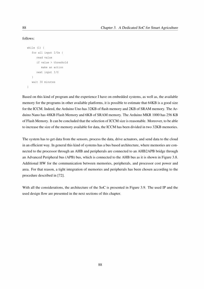
88 Chapter 3. A Dedicated SoC for Smart Agriculture
follows:
while (1) {
for all input I/Os {
read value
if value > threshold
make an action
next input I/O
}
wait 30 minutes
}
Based on this kind of program and the experience I have on embedded systems, as well as, the available
memory for the programs in other available platforms, it is possible to estimate that 64KB is a good size
for the ICCM. Indeed, the Arduino Uno has 32KB of flash memory and 2KB of SRAM memory. The Ar-
duino Nano has 48KB Flash Memory and 6KB of SRAM memory. The Arduino MKR 1000 has 256 KB
of Flash Memory. It can be concluded that the selection of ICCM size is reasonable. Moreover, to be able
to increase the size of the memory available for data, the ICCM has been divided in two 32KB memories.
The system has to get data from the sensors, process the data, drive actuators, and send data to the cloud
in an efficient way. In general this kind of systems has a bus based architecture, where memories are con-
nected to the processor through an AHB and peripherals are connected to an AHB2APB bridge through
an Advanced Peripheral bus (APB) bus, which is connected to the AHB bus as it is shown in Figure 3.8.
Additional HW for the communication between memories, peripherals, and processor cost power and
area. For that reason, a tight integration of memories and peripherals has been chosen according to the
procedure described in [72].
With all the considerations, the architecture of the SoC is presented in Figure 3.9. The used IP and the
used design flow are presented in the next sections of this chapter.
88
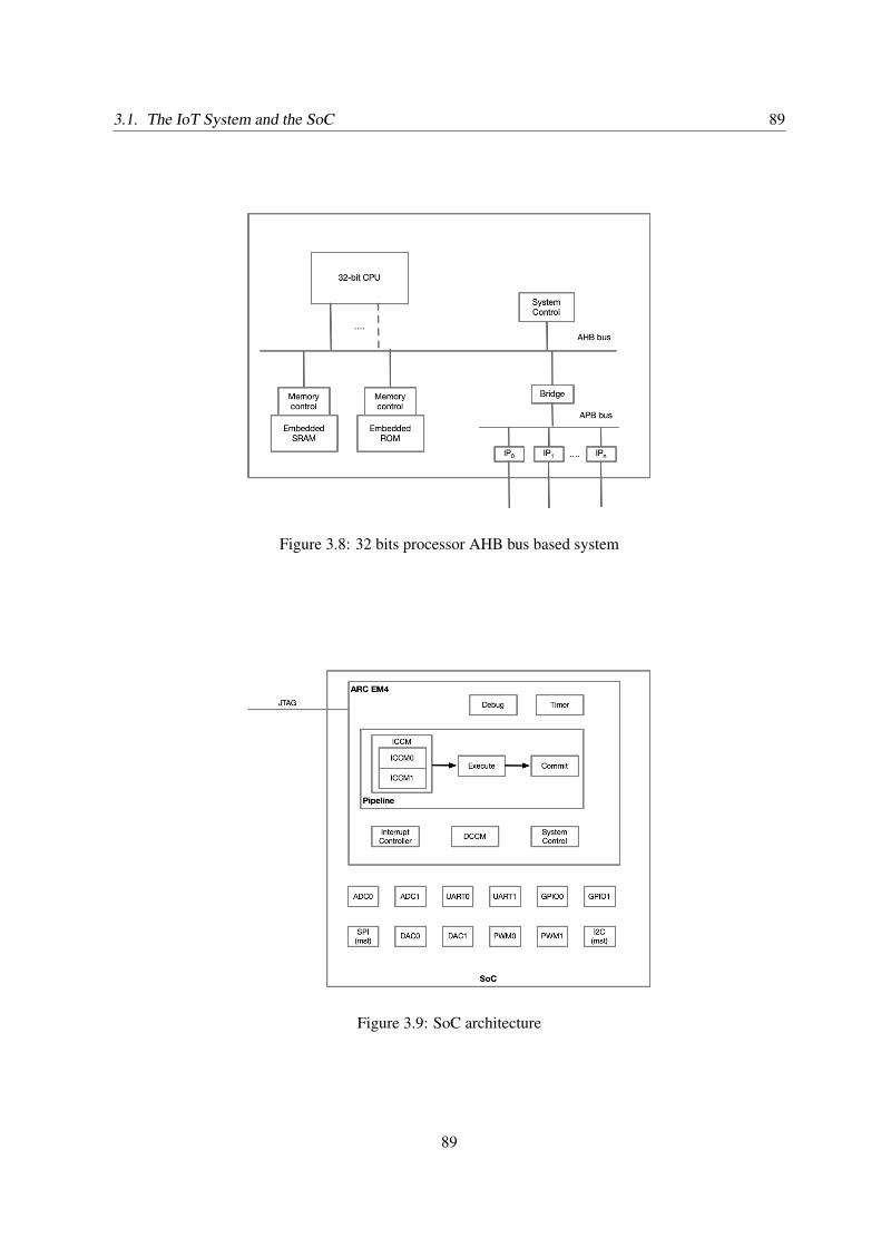
3.1. The IoT System and the SoC 89
Figure 3.8: 32 bits processor AHB bus based system
Figure 3.9: SoC architecture
89
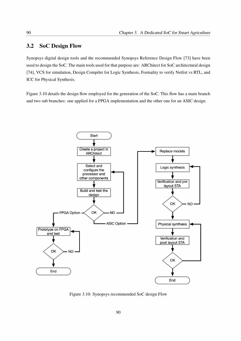
90 Chapter 3. A Dedicated SoC for Smart Agriculture
3.2 SoC Design Flow
Synopsys digital design tools and the recommended Synopsys Reference Design Flow [73] have been
used to design the SoC. The main tools used for that purpose are: ARChitect for SoC architectural design
[74], VCS for simulation, Design Compiler for Logic Synthesis, Formality to verify Netlist vs RTL, and
ICC for Physical Synthesis.
Figure 3.10 details the design flow employed for the generation of the SoC. This flow has a main branch
and two sub branches: one applied for a FPGA implementation and the other one for an ASIC design.
Figure 3.10: Synopsys recommended SoC design Flow
90
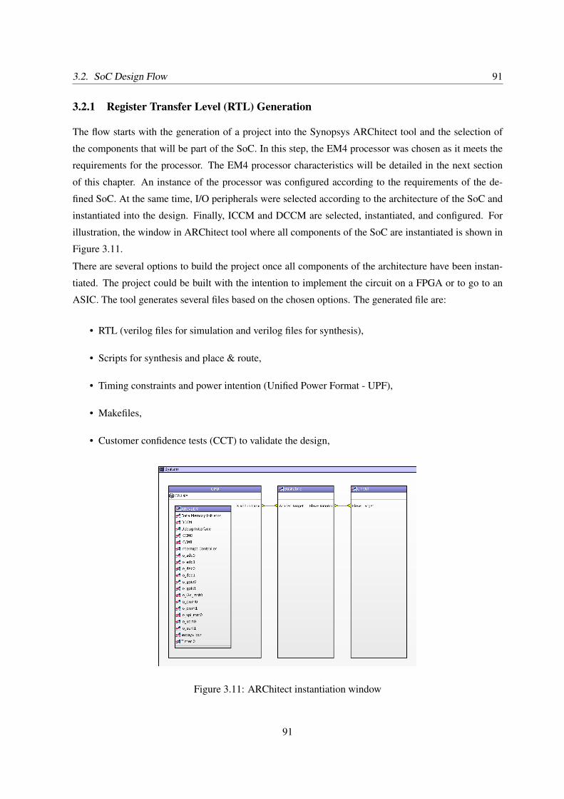
3.2. SoC Design Flow 91
3.2.1 Register Transfer Level (RTL) Generation
The flow starts with the generation of a project into the Synopsys ARChitect tool and the selection of
the components that will be part of the SoC. In this step, the EM4 processor was chosen as it meets the
requirements for the processor. The EM4 processor characteristics will be detailed in the next section
of this chapter. An instance of the processor was configured according to the requirements of the de-
fined SoC. At the same time, I/O peripherals were selected according to the architecture of the SoC and
instantiated into the design. Finally, ICCM and DCCM are selected, instantiated, and configured. For
illustration, the window in ARChitect tool where all components of the SoC are instantiated is shown in
Figure 3.11.
There are several options to build the project once all components of the architecture have been instan-
tiated. The project could be built with the intention to implement the circuit on a FPGA or to go to an
ASIC. The tool generates several files based on the chosen options. The generated file are:
• RTL (verilog files for simulation and verilog files for synthesis),
• Scripts for synthesis and place & route,
• Timing constraints and power intention (Unified Power Format - UPF),
• Makefiles,
• Customer confidence tests (CCT) to validate the design,
Figure 3.11: ARChitect instantiation window
91
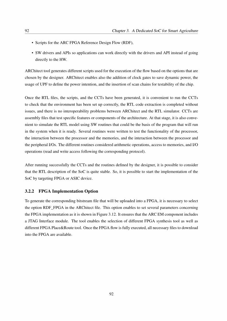
92 Chapter 3. A Dedicated SoC for Smart Agriculture
• Scripts for the ARC FPGA Reference Design Flow (RDF),
• SW drivers and APIs so applications can work directly with the drivers and API instead of going
directly to the HW.
ARChitect tool generates different scripts used for the execution of the flow based on the options that are
chosen by the designer. ARChitect enables also the addition of clock gates to save dynamic power, the
usage of UPF to define the power intention, and the insertion of scan chains for testability of the chip.
Once the RTL files, the scripts, and the CCTs have been generated, it is convenient to run the CCTs
to check that the environment has been set up correctly, the RTL code extraction is completed without
issues, and there is no interoperability problems between ARChitect and the RTL simulator. CCTs are
assembly files that test specific features or components of the architecture. At that stage, it is also conve-
nient to simulate the RTL model using SW routines that could be the basis of the program that will run
in the system when it is ready. Several routines were written to test the functionality of the processor,
the interaction between the processor and the memories, and the interaction between the processor and
the peripheral I/Os. The different routines considered arithmetic operations, access to memories, and I/O
operations (read and write access following the corresponding protocol).
After running successfully the CCTs and the routines defined by the designer, it is possible to consider
that the RTL description of the SoC is quite stable. So, it is possible to start the implementation of the
SoC by targeting FPGA or ASIC device.
3.2.2 FPGA Implementation Option
To generate the corresponding bitstream file that will be uploaded into a FPGA, it is necessary to select
the option RDF_FPGA in the ARChitect file. This option enables to set several parameters concerning
the FPGA implementation as it is shown in Figure 3.12. It ensures that the ARC EM component includes
a JTAG Interface module. The tool enables the selection of different FPGA synthesis tool as well as
different FPGA Place&Route tool. Once the FPGA flow is fully executed, all necessary files to download
into the FPGA are available.
92
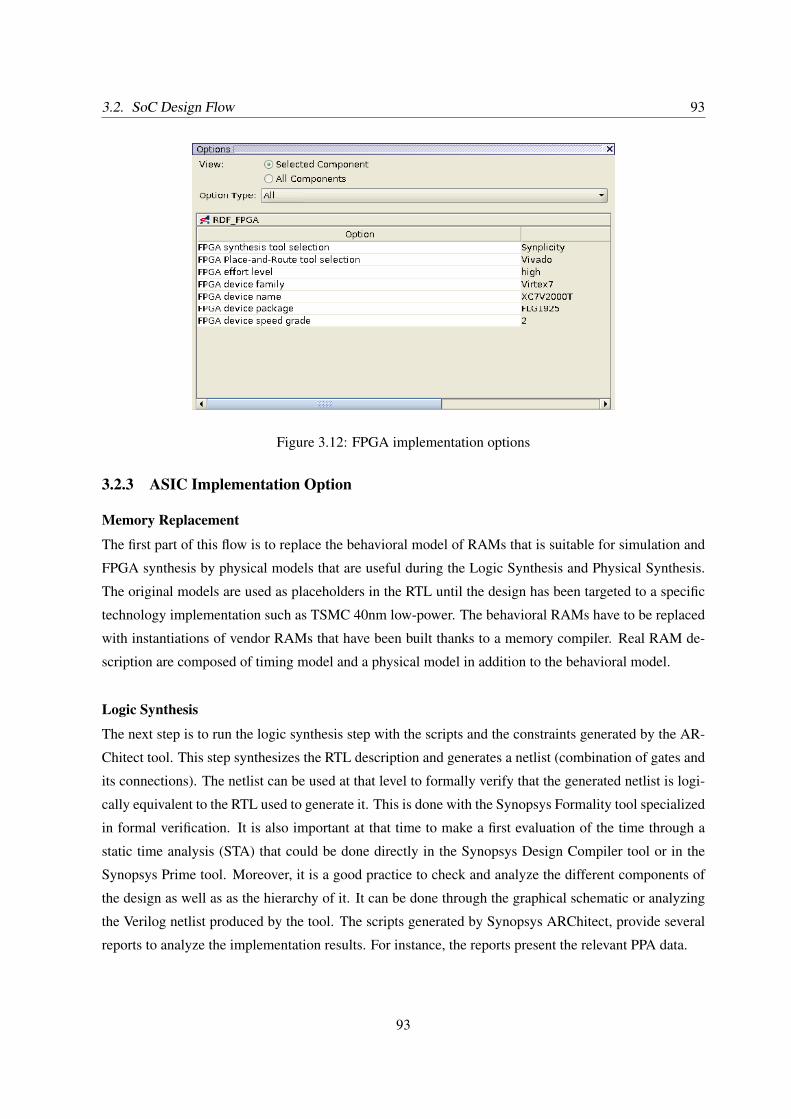
3.2. SoC Design Flow 93
Figure 3.12: FPGA implementation options
3.2.3 ASIC Implementation Option
Memory Replacement
The first part of this flow is to replace the behavioral model of RAMs that is suitable for simulation and
FPGA synthesis by physical models that are useful during the Logic Synthesis and Physical Synthesis.
The original models are used as placeholders in the RTL until the design has been targeted to a specific
technology implementation such as TSMC 40nm low-power. The behavioral RAMs have to be replaced
with instantiations of vendor RAMs that have been built thanks to a memory compiler. Real RAM de-
scription are composed of timing model and a physical model in addition to the behavioral model.
Logic Synthesis
The next step is to run the logic synthesis step with the scripts and the constraints generated by the AR-
Chitect tool. This step synthesizes the RTL description and generates a netlist (combination of gates and
its connections). The netlist can be used at that level to formally verify that the generated netlist is logi-
cally equivalent to the RTL used to generate it. This is done with the Synopsys Formality tool specialized
in formal verification. It is also important at that time to make a first evaluation of the time through a
static time analysis (STA) that could be done directly in the Synopsys Design Compiler tool or in the
Synopsys Prime tool. Moreover, it is a good practice to check and analyze the different components of
the design as well as as the hierarchy of it. It can be done through the graphical schematic or analyzing
the Verilog netlist produced by the tool. The scripts generated by Synopsys ARChitect, provide several
reports to analyze the implementation results. For instance, the reports present the relevant PPA data.
93
94 Chapter 3. A Dedicated SoC for Smart Agriculture
The generated netlist has two main blocks on the top level: one block containing the memories, u_srams
and another one containing the rest of the chip (cpu, peripherals, jtag, etc.), u_cpu. Figure 3.13 shows
the schematic of the top level of the SoC after synthesis. The two main blocks are highlighted. Figures
3.14 and 3.15 present the details of each block. The characteristics of the SoC at that level of the design
are summarized in Table 3.1
Parameter Value Unit
# of ports 44048 N/A
# of nets 89095 N/A
# of cells 45965 N/A
# of combinational cells 36356 N/A
# of sequential cells 8608 N/A
# of memories 4 N/A
# of buf/inv 9340 N/A
Combinational area 39610.620467 um2
Buf/Inv area 5767.750978 um2
Non combinational area 40935.738191 um
Memories area 284252.375000 um2
Total cell area 364798.733657 um2
Dynamic power 2.7433 mw
Leakage Power 207.2277 uw
Critical Path Length - mem2reg 4.26 ns
Critical Path Length - reg2mem 4.31 ns
Critical Path Length - reg2reg 4.62 ns
Critical Path Length - in2reg 1.14 ns
Critical Path Length - reg2out 1.30 ns
Table 3.1: Architecture features after synthesis
Physical SynthesisDuring the physical synthesis, the netlist is converted into a layout. For this step, the Synopsys tool ICC2
was applied. The physical synthesis is composed by three main steps: Floorplanning, Place and Route.
A layout is in general composed by three types of reference cells:
• Macro cells (ROMs, RAMs, physical IP blocks),
• Standard cells (nand2, inv, buff, ...),
• Pad cells (input, output, bidirectional, Vdd, Vss).
The placement of the Macro and Pad cells have to be selected by the designer during the floorplanning
step. The main objective is to minimize the length of connection between the different blocks. The
94
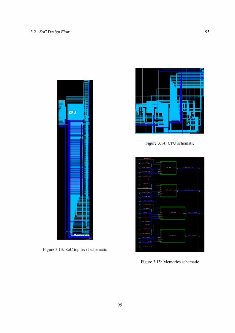
3.2. SoC Design Flow 95
Figure 3.13: SoC top level schematic
Figure 3.14: CPU schematic
Figure 3.15: Memories schematic
95
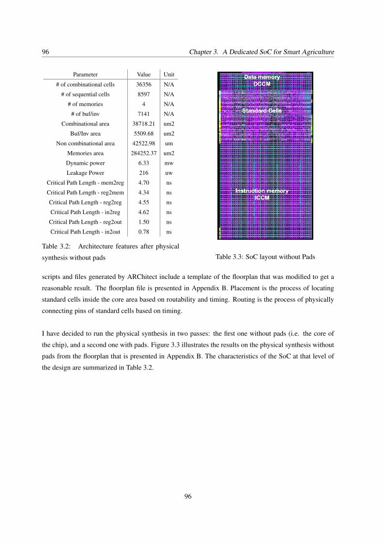
96 Chapter 3. A Dedicated SoC for Smart Agriculture
Parameter Value Unit
# of combinational cells 36356 N/A
# of sequential cells 8597 N/A
# of memories 4 N/A
# of buf/inv 7141 N/A
Combinational area 38718.21 um2
Buf/Inv area 5509.68 um2
Non combinational area 42522.98 um
Memories area 284252.37 um2
Dynamic power 6.33 mw
Leakage Power 216 uw
Critical Path Length - mem2reg 4.70 ns
Critical Path Length - reg2mem 4.34 ns
Critical Path Length - reg2reg 4.55 ns
Critical Path Length - in2reg 4.62 ns
Critical Path Length - reg2out 1.50 ns
Critical Path Length - in2out 0.78 ns
Table 3.2: Architecture features after physical
synthesis without pads Table 3.3: SoC layout without Pads
scripts and files generated by ARChitect include a template of the floorplan that was modified to get a
reasonable result. The floorplan file is presented in Appendix B. Placement is the process of locating
standard cells inside the core area based on routability and timing. Routing is the process of physically
connecting pins of standard cells based on timing.
I have decided to run the physical synthesis in two passes: the first one without pads (i.e. the core of
the chip), and a second one with pads. Figure 3.3 illustrates the results on the physical synthesis without
pads from the floorplan that is presented in Appendix B. The characteristics of the SoC at that level of
the design are summarized in Table 3.2.
96
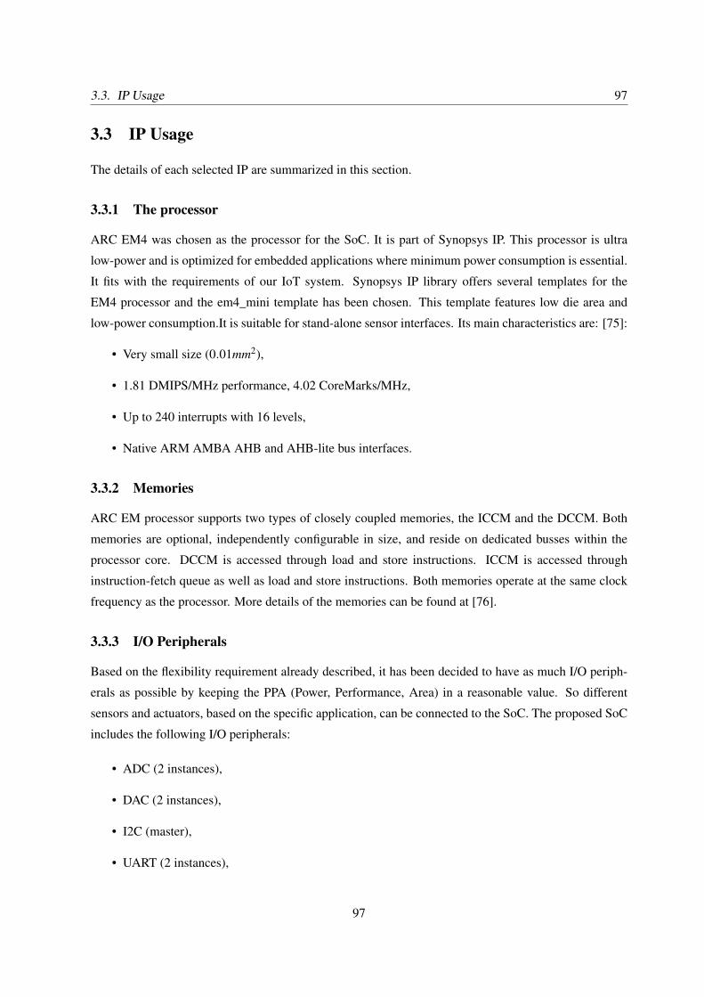
3.3. IP Usage 97
3.3 IP Usage
The details of each selected IP are summarized in this section.
3.3.1 The processor
ARC EM4 was chosen as the processor for the SoC. It is part of Synopsys IP. This processor is ultra
low-power and is optimized for embedded applications where minimum power consumption is essential.
It fits with the requirements of our IoT system. Synopsys IP library offers several templates for the
EM4 processor and the em4_mini template has been chosen. This template features low die area and
low-power consumption.It is suitable for stand-alone sensor interfaces. Its main characteristics are: [75]:
• Very small size (0.01mm2),
• 1.81 DMIPS/MHz performance, 4.02 CoreMarks/MHz,
• Up to 240 interrupts with 16 levels,
• Native ARM AMBA AHB and AHB-lite bus interfaces.
3.3.2 Memories
ARC EM processor supports two types of closely coupled memories, the ICCM and the DCCM. Both
memories are optional, independently configurable in size, and reside on dedicated busses within the
processor core. DCCM is accessed through load and store instructions. ICCM is accessed through
instruction-fetch queue as well as load and store instructions. Both memories operate at the same clock
frequency as the processor. More details of the memories can be found at [76].
3.3.3 I/O Peripherals
Based on the flexibility requirement already described, it has been decided to have as much I/O periph-
erals as possible by keeping the PPA (Power, Performance, Area) in a reasonable value. So different
sensors and actuators, based on the specific application, can be connected to the SoC. The proposed SoC
includes the following I/O peripherals:
• ADC (2 instances),
• DAC (2 instances),
• I2C (master),
• UART (2 instances),
97
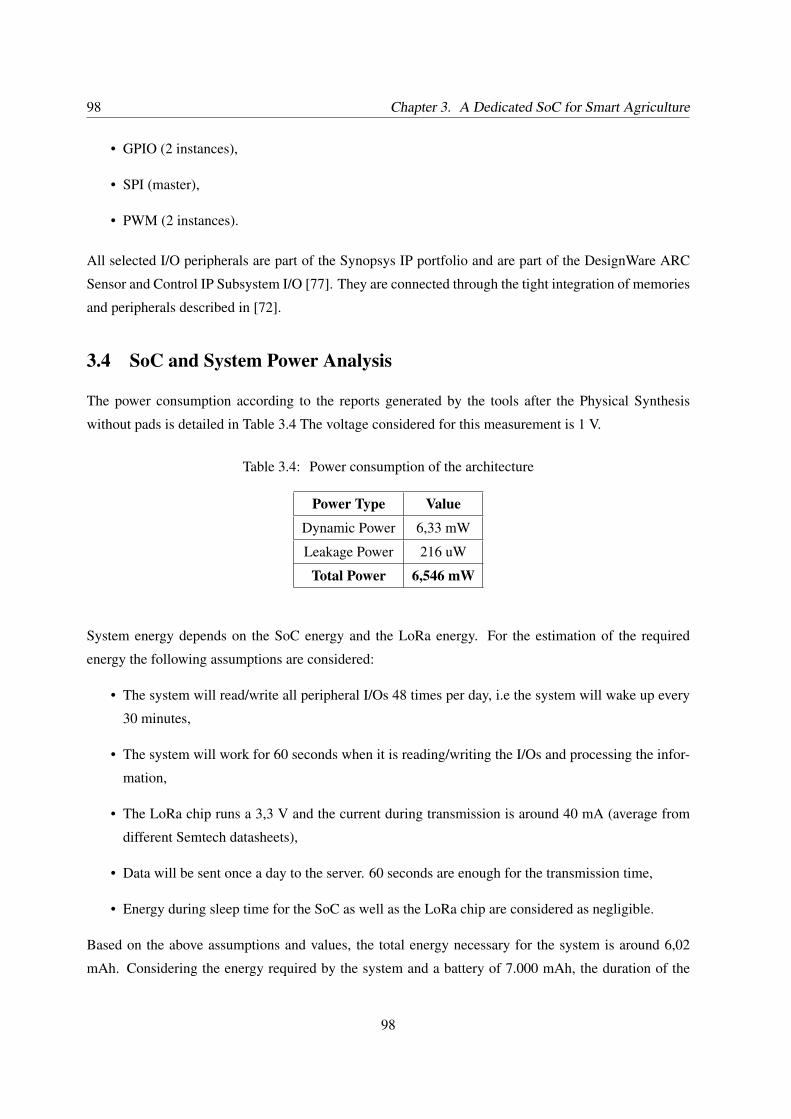
98 Chapter 3. A Dedicated SoC for Smart Agriculture
• GPIO (2 instances),
• SPI (master),
• PWM (2 instances).
All selected I/O peripherals are part of the Synopsys IP portfolio and are part of the DesignWare ARC
Sensor and Control IP Subsystem I/O [77]. They are connected through the tight integration of memories
and peripherals described in [72].
3.4 SoC and System Power Analysis
The power consumption according to the reports generated by the tools after the Physical Synthesis
without pads is detailed in Table 3.4 The voltage considered for this measurement is 1 V.
Table 3.4: Power consumption of the architecture
Power Type Value
Dynamic Power 6,33 mW
Leakage Power 216 uW
Total Power 6,546 mW
System energy depends on the SoC energy and the LoRa energy. For the estimation of the required
energy the following assumptions are considered:
• The system will read/write all peripheral I/Os 48 times per day, i.e the system will wake up every
30 minutes,
• The system will work for 60 seconds when it is reading/writing the I/Os and processing the infor-
mation,
• The LoRa chip runs a 3,3 V and the current during transmission is around 40 mA (average from
different Semtech datasheets),
• Data will be sent once a day to the server. 60 seconds are enough for the transmission time,
• Energy during sleep time for the SoC as well as the LoRa chip are considered as negligible.
Based on the above assumptions and values, the total energy necessary for the system is around 6,02
mAh. Considering the energy required by the system and a battery of 7.000 mAh, the duration of the
98
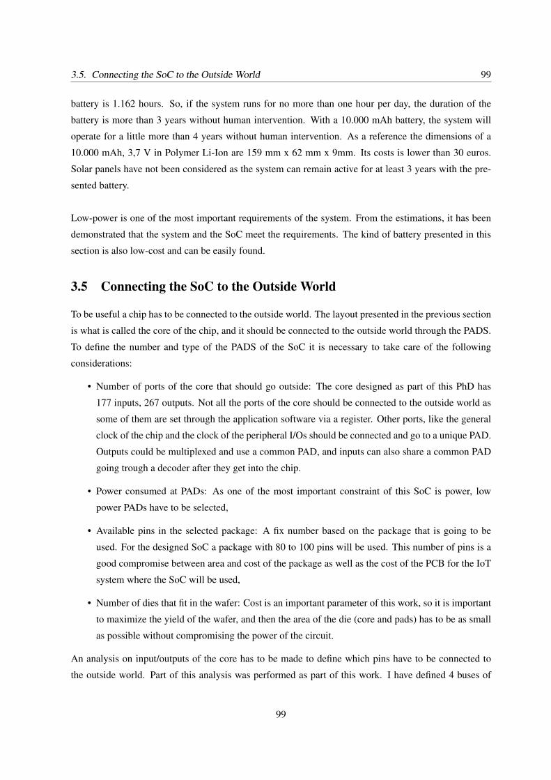
3.5. Connecting the SoC to the Outside World 99
battery is 1.162 hours. So, if the system runs for no more than one hour per day, the duration of the
battery is more than 3 years without human intervention. With a 10.000 mAh battery, the system will
operate for a little more than 4 years without human intervention. As a reference the dimensions of a
10.000 mAh, 3,7 V in Polymer Li-Ion are 159 mm x 62 mm x 9mm. Its costs is lower than 30 euros.
Solar panels have not been considered as the system can remain active for at least 3 years with the pre-
sented battery.
Low-power is one of the most important requirements of the system. From the estimations, it has been
demonstrated that the system and the SoC meet the requirements. The kind of battery presented in this
section is also low-cost and can be easily found.
3.5 Connecting the SoC to the Outside World
To be useful a chip has to be connected to the outside world. The layout presented in the previous section
is what is called the core of the chip, and it should be connected to the outside world through the PADS.
To define the number and type of the PADS of the SoC it is necessary to take care of the following
considerations:
• Number of ports of the core that should go outside: The core designed as part of this PhD has
177 inputs, 267 outputs. Not all the ports of the core should be connected to the outside world as
some of them are set through the application software via a register. Other ports, like the general
clock of the chip and the clock of the peripheral I/Os should be connected and go to a unique PAD.
Outputs could be multiplexed and use a common PAD, and inputs can also share a common PAD
going trough a decoder after they get into the chip.
• Power consumed at PADs: As one of the most important constraint of this SoC is power, low
power PADs have to be selected,
• Available pins in the selected package: A fix number based on the package that is going to be
used. For the designed SoC a package with 80 to 100 pins will be used. This number of pins is a
good compromise between area and cost of the package as well as the cost of the PCB for the IoT
system where the SoC will be used,
• Number of dies that fit in the wafer: Cost is an important parameter of this work, so it is important
to maximize the yield of the wafer, and then the area of the die (core and pads) has to be as small
as possible without compromising the power of the circuit.
An analysis on input/outputs of the core has to be made to define which pins have to be connected to
the outside world. Part of this analysis was performed as part of this work. I have defined 4 buses of
99
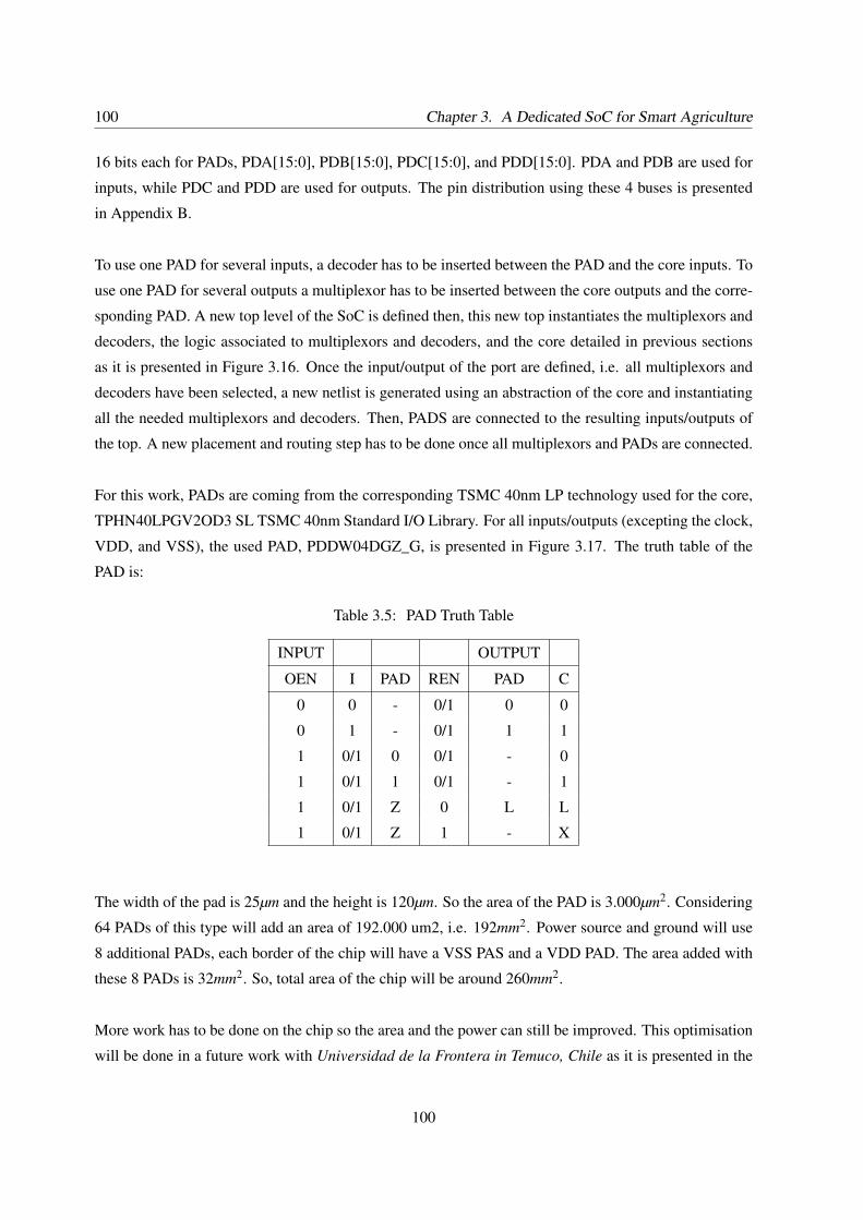
100 Chapter 3. A Dedicated SoC for Smart Agriculture
16 bits each for PADs, PDA[15:0], PDB[15:0], PDC[15:0], and PDD[15:0]. PDA and PDB are used for
inputs, while PDC and PDD are used for outputs. The pin distribution using these 4 buses is presented
in Appendix B.
To use one PAD for several inputs, a decoder has to be inserted between the PAD and the core inputs. To
use one PAD for several outputs a multiplexor has to be inserted between the core outputs and the corre-
sponding PAD. A new top level of the SoC is defined then, this new top instantiates the multiplexors and
decoders, the logic associated to multiplexors and decoders, and the core detailed in previous sections
as it is presented in Figure 3.16. Once the input/output of the port are defined, i.e. all multiplexors and
decoders have been selected, a new netlist is generated using an abstraction of the core and instantiating
all the needed multiplexors and decoders. Then, PADS are connected to the resulting inputs/outputs of
the top. A new placement and routing step has to be done once all multiplexors and PADs are connected.
For this work, PADs are coming from the corresponding TSMC 40nm LP technology used for the core,
TPHN40LPGV2OD3 SL TSMC 40nm Standard I/O Library. For all inputs/outputs (excepting the clock,
VDD, and VSS), the used PAD, PDDW04DGZ_G, is presented in Figure 3.17. The truth table of the
PAD is:
Table 3.5: PAD Truth Table
INPUT OUTPUT
OEN I PAD REN PAD C
0 0 - 0/1 0 0
0 1 - 0/1 1 1
1 0/1 0 0/1 - 0
1 0/1 1 0/1 - 1
1 0/1 Z 0 L L
1 0/1 Z 1 - X
The width of the pad is 25µm and the height is 120µm. So the area of the PAD is 3.000µm2. Considering
64 PADs of this type will add an area of 192.000 um2, i.e. 192mm2. Power source and ground will use
8 additional PADs, each border of the chip will have a VSS PAS and a VDD PAD. The area added with
these 8 PADs is 32mm2. So, total area of the chip will be around 260mm2.
More work has to be done on the chip so the area and the power can still be improved. This optimisation
will be done in a future work with Universidad de la Frontera in Temuco, Chile as it is presented in the
100
3.5. Connecting the SoC to the Outside World 101
next chapter.
Figure 3.16: Top level of the SoC including muxes and decoders
Figure 3.17: PAD schematic
101
102 Chapter 3. A Dedicated SoC for Smart Agriculture
102
CHAPTER
4THE AGRIFOOD
COMMUNITY
Sommaire4.1 The Community I have Found and Where It is Now . . . . . . . . . . . . . . . . . 104
4.1.1 Seasonal School . . . . . . . . . . . . . . . . . . . . . . . . . . . . . . . . . 104
4.1.2 FoodCAS Community . . . . . . . . . . . . . . . . . . . . . . . . . . . . . . 107
4.2 How Technology Can Help to Feed the Humanity . . . . . . . . . . . . . . . . . . 108
4.3 My Contribution to the AgriFood Community . . . . . . . . . . . . . . . . . . . . 111
4.4 Next Steps and Future Research . . . . . . . . . . . . . . . . . . . . . . . . . . . . 114
4.4.1 Lack of Low-Power and Low-Cost Sensors . . . . . . . . . . . . . . . . . . . 115
4.4.2 Equation, model and interrelation of plant’s parameters . . . . . . . . . . . . . 115
4.4.3 Better understanding of plants growth for better IoT systems . . . . . . . . . . 118
4.4.4 Enhance capabilities of the SoC . . . . . . . . . . . . . . . . . . . . . . . . . 121
4.5 Conclusion . . . . . . . . . . . . . . . . . . . . . . . . . . . . . . . . . . . . . . . . 121
103
104 Chapter 4. The AgriFood Community
During my research work, I found that an AgriFood community was existing. I approached its members
and started to participate actively. The community has helped me to better understand the agribusiness
issues and how technology can help to address those issues and to feed the growing humanity. I also
found that a lot of research is being done by this community and several specialists are working on
different topics related to the agribusiness. In this chapter, I present the community and my contribution
to it. I also present how the technology can help to feed a growing humanity while keeping planetary
boundaries under control. Finally, I present the next steps of my work and the perspectives of this
research work.
4.1 The Community I have Found and Where It is Now
When I started my PhD, I have not only looked at the technology that was applied to agriculture but
also at the community that was around the topic. My first interaction with the community was in 2018
when I presented a paper in International Conference on Electronics, Circuits, and Systems (ICECS),
held in Bordeaux, France. A session related to IoT and food was specifically organized. Thus, I was
able to meet several researchers that were involved on technology for the agribusiness. At the end of
the session, I was invited to participate and to submit a paper to the next Circuits and Systems for better
quality foods (FoodCAS) conference that was going to be held at the next International Symposium on
Circuits and Systems (ISCAS) in Sapporo, Japan in 2019. Then, I submitted a paper to FoodCAS 2019,
which was accepted and presented. During FoodCAS 2019, I met additional people involved in the topic
and I started to participate in the community. I volunteered to be the Technical Program Committee
(TPC) Chair of FoodCAS 2020, held virtually in October 2020. Between the two FoodCAS editions, I
increased my participation and interest on the technology and its application to the agribusiness.
4.1.1 Seasonal School
In parallel with the preparation of FoodCAS 2020, I submitted to IEEE CASS (Circuits and Systems
Society) a proposal for a seasonal school on technology for the agribusiness, entitled Technology and
Agribusiness: How Technology is Impacting Agribusiness. It was held virtually in November 2020.
19 speakers presented their work on different topics related to the technology for agribusiness and the
agronomy. A flyer of the school is presented in Figure 4.1. The following talks were presented at the
104
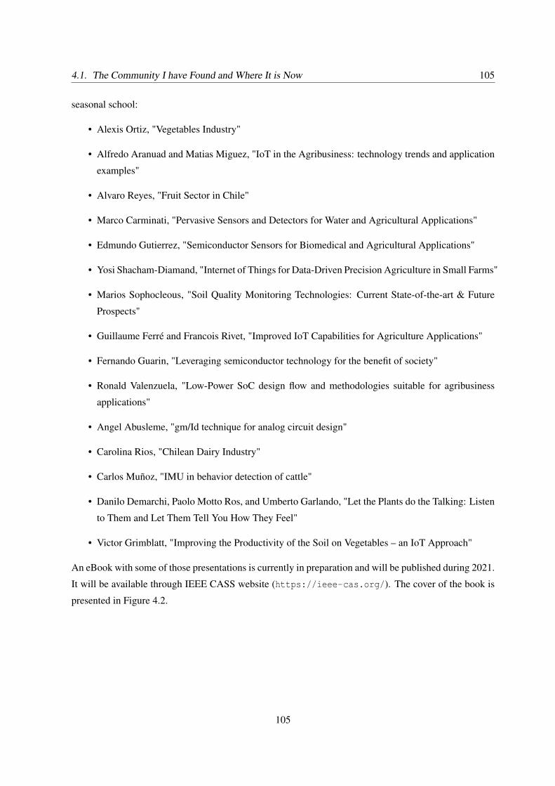
4.1. The Community I have Found and Where It is Now 105
seasonal school:
• Alexis Ortiz, "Vegetables Industry"
• Alfredo Aranuad and Matias Miguez, "IoT in the Agribusiness: technology trends and application
examples"
• Alvaro Reyes, "Fruit Sector in Chile"
• Marco Carminati, "Pervasive Sensors and Detectors for Water and Agricultural Applications"
• Edmundo Gutierrez, "Semiconductor Sensors for Biomedical and Agricultural Applications"
• Yosi Shacham-Diamand, "Internet of Things for Data-Driven Precision Agriculture in Small Farms"
• Marios Sophocleous, "Soil Quality Monitoring Technologies: Current State-of-the-art & Future
Prospects"
• Guillaume Ferré and Francois Rivet, "Improved IoT Capabilities for Agriculture Applications"
• Fernando Guarin, "Leveraging semiconductor technology for the benefit of society"
• Ronald Valenzuela, "Low-Power SoC design flow and methodologies suitable for agribusiness
applications"
• Angel Abusleme, "gm/Id technique for analog circuit design"
• Carolina Rios, "Chilean Dairy Industry"
• Carlos Muñoz, "IMU in behavior detection of cattle"
• Danilo Demarchi, Paolo Motto Ros, and Umberto Garlando, "Let the Plants do the Talking: Listen
to Them and Let Them Tell You How They Feel"
• Victor Grimblatt, "Improving the Productivity of the Soil on Vegetables – an IoT Approach"
An eBook with some of those presentations is currently in preparation and will be published during 2021.
It will be available through IEEE CASS website (https://ieee-cas.org/). The cover of the book is
presented in Figure 4.2.
105
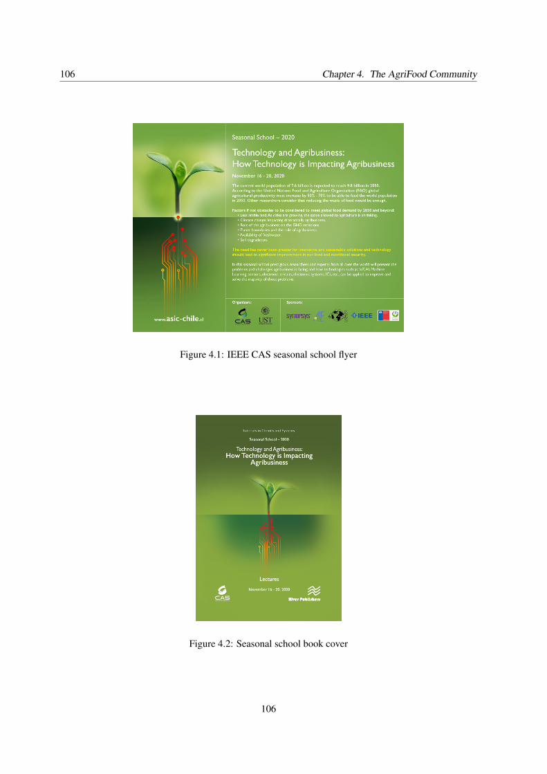
106 Chapter 4. The AgriFood Community
Figure 4.1: IEEE CAS seasonal school flyer
Figure 4.2: Seasonal school book cover
106
4.1. The Community I have Found and Where It is Now 107
4.1.2 FoodCAS Community
FoodCAS 2020 was held virtually with a greater attendance. The program of the conference is presented
in Figure 4.3. During the conference, I was invited to give an overview of IoT and the agribusiness. At
the end of the conference, I was invited to co-chair the FoodCAS 2021 edition, held virtually in May
2021. During this edition, I presented the different actions that the community was planning to do:
• CASS Special Interest Group (SIG) - Electronics for Agrifood: The creation of the SIG was
approved by CASS and I chair this group for the next 2 years. The group has already over 30
members interested in the different topics the SIG is going to address,
• 2nd Seasonal School on Agribusiness and Technology: The name of the 2nd school is Feeding a
growing population. During the school the agribusineess issues to feed a growing population will
be discussed from the agricultural and the circuits and systems prospective. The topics covered by
this second edition of the school will be: meat industry, dairy industry, fertilization, sensors for
agriculture, soil analysis in real-time (analyzed deeply in this work), electronics for agrifood, the
growth and health of plants (analyzed deeply in this work), aquaculture, and food waste process
and reutilization. This second edition was approved by CASS with the highest score among all
proposed seasonal schools and will be held virtually in November 2021,
• Agrifood conference: Yearly conference covering important topics for the food and agriculture
domains. The next edition will be held in August - September 2022 time frame in Torino, Italy.
The 2023 edition is scheduled to be held in Uruguay,
• Agrifood CASIF (Industry Forum): The objective of the forum is to increase the interaction
between the Agrifood research community with the industry,
• Transactions on Agrifood Electronics (TAFE): Specialized journal on electronics for Agrifood.
TAFE will be launched during 2022 Agrifood Conference.
New activities will be proposed in the future and the group will include not only people from the elec-
tronics and systems world, but also from agronomy and food industry.
107
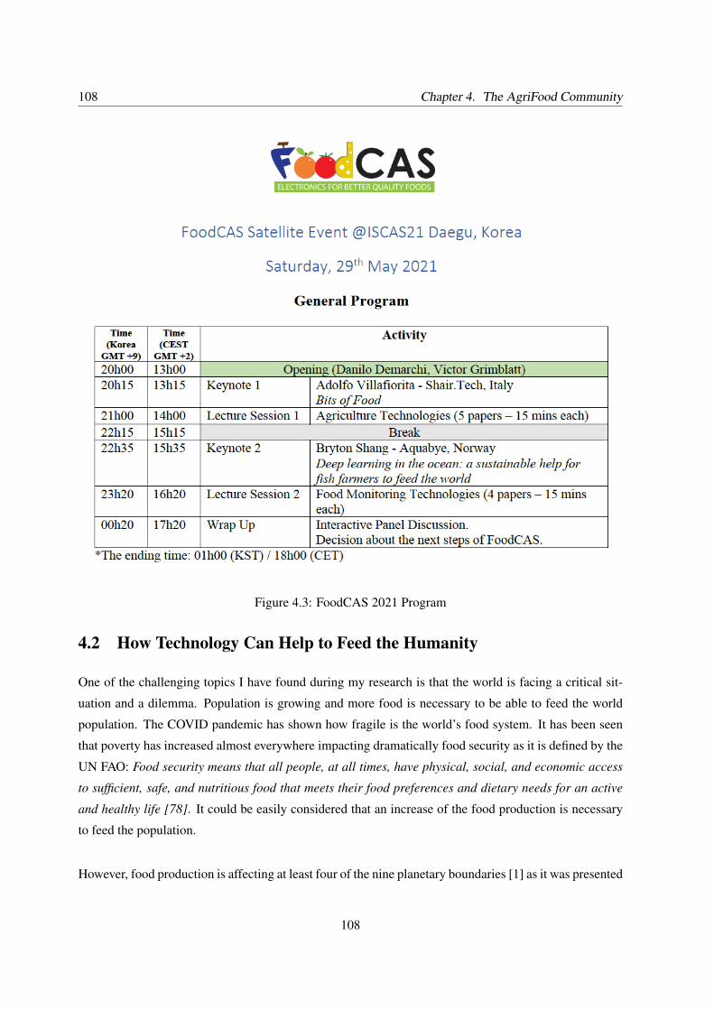
108 Chapter 4. The AgriFood Community
Figure 4.3: FoodCAS 2021 Program
4.2 How Technology Can Help to Feed the Humanity
One of the challenging topics I have found during my research is that the world is facing a critical sit-
uation and a dilemma. Population is growing and more food is necessary to be able to feed the world
population. The COVID pandemic has shown how fragile is the world’s food system. It has been seen
that poverty has increased almost everywhere impacting dramatically food security as it is defined by the
UN FAO: Food security means that all people, at all times, have physical, social, and economic access
to sufficient, safe, and nutritious food that meets their food preferences and dietary needs for an active
and healthy life [78]. It could be easily considered that an increase of the food production is necessary
to feed the population.
However, food production is affecting at least four of the nine planetary boundaries [1] as it was presented
108
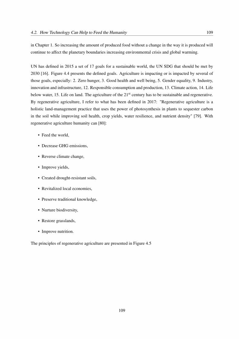
4.2. How Technology Can Help to Feed the Humanity 109
in Chapter 1. So increasing the amount of produced food without a change in the way it is produced will
continue to affect the planetary boundaries increasing environmental crisis and global warming.
UN has defined in 2015 a set of 17 goals for a sustainable world, the UN SDG that should be met by
2030 [16]. Figure 4.4 presents the defined goals. Agriculture is impacting or is impacted by several of
those goals, especially: 2. Zero hunger, 3. Good health and well being, 5. Gender equality, 9. Industry,
innovation and infrastructure, 12. Responsible consumption and production, 13. Climate action, 14. Life
below water, 15. Life on land. The agriculture of the 21st century has to be sustainable and regenerative.
By regenerative agriculture, I refer to what has been defined in 2017: "Regenerative agriculture is a
holistic land-management practice that uses the power of photosynthesis in plants to sequester carbon
in the soil while improving soil health, crop yields, water resilience, and nutrient density" [79]. With
regenerative agriculture humanity can [80]:
• Feed the world,
• Decrease GHG emissions,
• Reverse climate change,
• Improve yields,
• Created drought-resistant soils,
• Revitalized local economies,
• Preserve traditional knowledge,
• Nurture biodiversity,
• Restore grasslands,
• Improve nutrition.
The principles of regenerative agriculture are presented in Figure 4.5
109
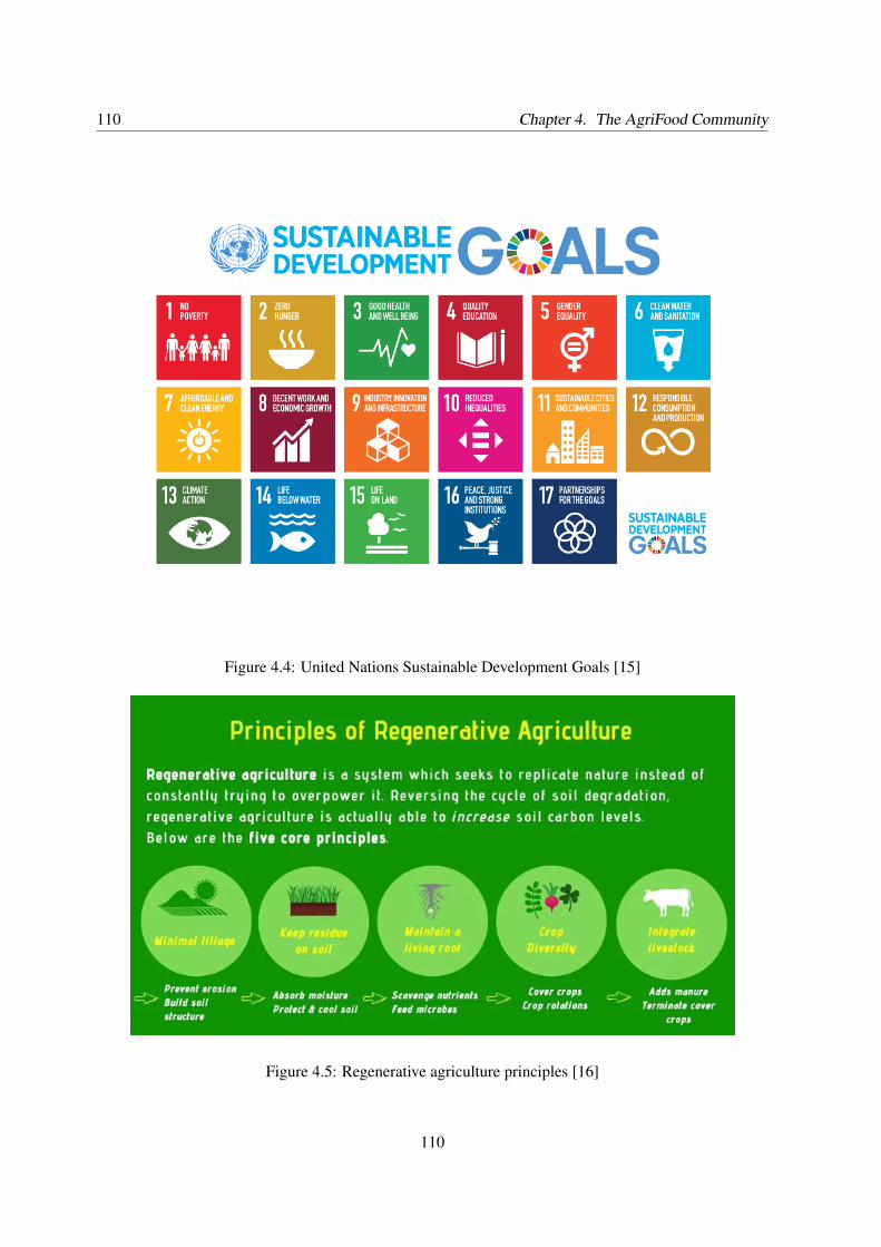
110 Chapter 4. The AgriFood Community
Figure 4.4: United Nations Sustainable Development Goals [15]
Figure 4.5: Regenerative agriculture principles [16]
110
4.3. My Contribution to the AgriFood Community 111
The presented dilemma is how to feed a growing population without affecting the planetary boundaries
and even how to decrease the impact of the agribusiness in the boundaries. The way food is produced
is affecting negatively some of the 17 UN SDG, so they should be considered when analyzing the prob-
lem. It is also necessary to look at the regenerative agriculture principles when looking at the agriculture
situation and how to solve the different issues presented in this work. Technology could be one of the
solutions. However, it has to be applied understanding the agribusiness as well as the physical and chem-
ical processes that impact the growth and health of plants and thus their productivity. For example, the
amount of water consumed by a plant depends on its stage of development and the texture of the soil.
Technology without a thorough understanding of plant growth is useless and even counterproductive.
Systems that will be proposed for the agriculture should take into account how a plant grows and how
to impact on productivity considering at the same the impact of the productivity in the planet and the
Humanity.
In this research work, I have studied the behavior of plants and the different parameters that impact its
growth and health. I have designed a system that measures part of those parameters and defines when
irrigation and fertilization is necessary. Over irrigation and over fertilization not only impact plants
growth but also the Earth. Under irrigation and under fertilization are also affecting plants and the Earth.
So, the good and right point has to be reached. Technology can be the key factor to make the precise
irrigation and fertilization a reality.
4.3 My Contribution to the AgriFood Community
During my research work, I have found several topics which kept my attention. My research has always
been oriented by those topics and how I was able to influence them. These topics are:
• Agriculture contribution to global warning, other planet issues and the UN SDG,
• Regenerative agriculture,
• Lack of IoT and electronic systems considering the process of plants’ growth,
• Lack of IoT and electronic systems for small and medium farmers,
• Lack of interaction between farmers and agronomists with electronics and system engineers,
• Low level of technification of the agribusiness, especially small and medium farmers.
As presented in Chapter 1, agriculture is an important contributor of global warming and is responsible
for least four planet boundaries that are at risk level. Agriculture is also impacting negatively several of
111
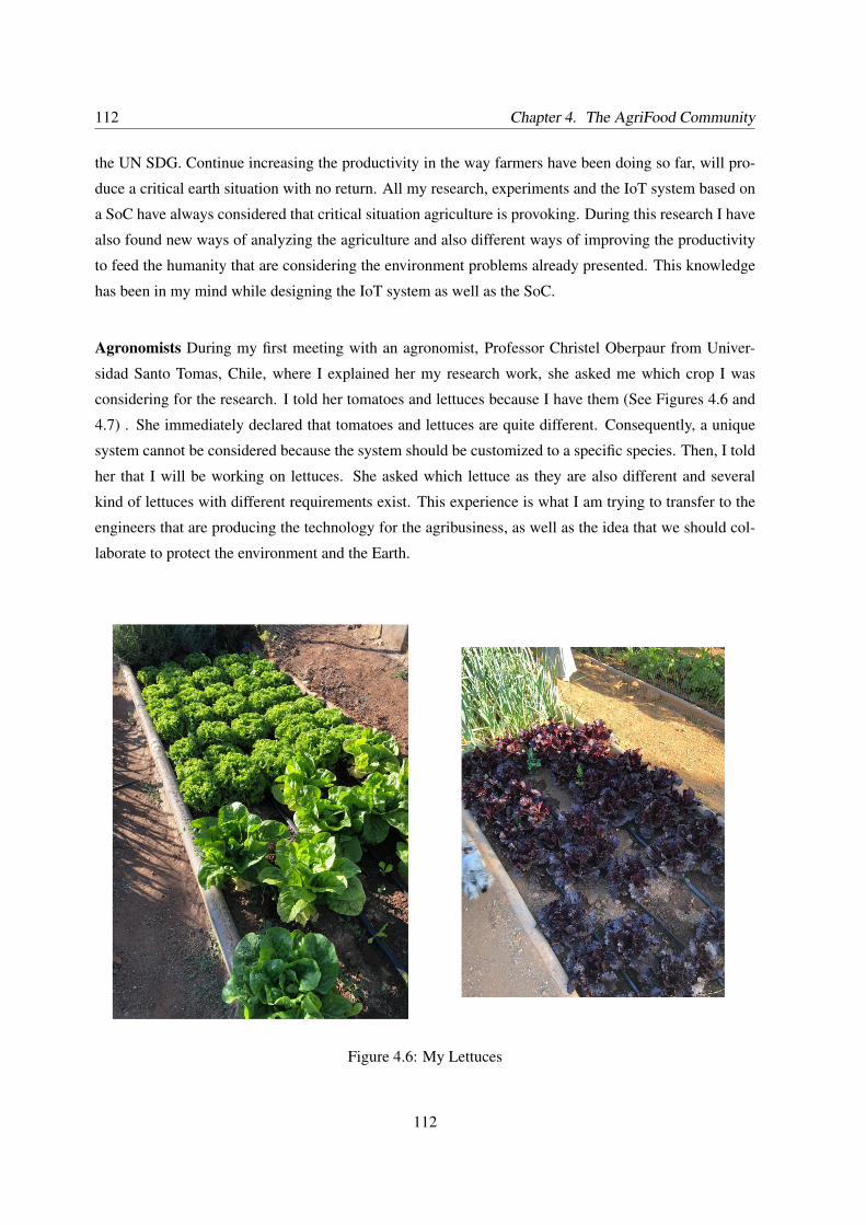
112 Chapter 4. The AgriFood Community
the UN SDG. Continue increasing the productivity in the way farmers have been doing so far, will pro-
duce a critical earth situation with no return. All my research, experiments and the IoT system based on
a SoC have always considered that critical situation agriculture is provoking. During this research I have
also found new ways of analyzing the agriculture and also different ways of improving the productivity
to feed the humanity that are considering the environment problems already presented. This knowledge
has been in my mind while designing the IoT system as well as the SoC.
Agronomists During my first meeting with an agronomist, Professor Christel Oberpaur from Univer-
sidad Santo Tomas, Chile, where I explained her my research work, she asked me which crop I was
considering for the research. I told her tomatoes and lettuces because I have them (See Figures 4.6 and
4.7) . She immediately declared that tomatoes and lettuces are quite different. Consequently, a unique
system cannot be considered because the system should be customized to a specific species. Then, I told
her that I will be working on lettuces. She asked which lettuce as they are also different and several
kind of lettuces with different requirements exist. This experience is what I am trying to transfer to the
engineers that are producing the technology for the agribusiness, as well as the idea that we should col-
laborate to protect the environment and the Earth.
Figure 4.6: My Lettuces
112
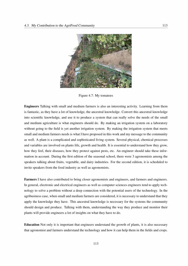
4.3. My Contribution to the AgriFood Community 113
Figure 4.7: My tomatoes
Engineers Talking with small and medium farmers is also an interesting activity. Learning from them
is fantastic, as they have a lot of knowledge, the ancestral knowledge. Convert this ancestral knowledge
into scientific knowledge, and use it to produce a system that can really solve the needs of the small
and medium agriculture is what engineers should do. By making an irrigation system on a laboratory
without going to the field is yet another irrigation system. By making the irrigation system that meets
small and medium farmers needs is what I have proposed in this work and my message to the community
as well. A plant is a complicated and sophisticated living system. Several physical, chemical processes
and variables are involved on plants life, growth and health. It is essential to understand how they grow,
how they feel, their diseases, how they protect against pests, etc. An engineer should take these infor-
mation in account. During the first edition of the seasonal school, there were 3 agronomists among the
speakers talking about fruits, vegetable, and dairy industries. For the second edition, it is scheduled to
invite speakers from the food industry as well as agronomists.
Farmers I have also contributed to bring closer agronomists and engineers, and farmers and engineers.
In general, electronic and electrical engineers as well as computer sciences engineers tend to apply tech-
nology to solve a problem without a deep connection with the potential users of the technology. In the
agribusiness case, when small and medium farmers are considered, it is necessary to understand that they
apply the knowledge they have. This ancestral knowledge is necessary for the systems the community
should design and produce. Talking with them, understanding the way they produce and monitor their
plants will provide engineers a lot of insights on what they have to do.
Education Not only it is important that engineers understand the growth of plants, it is also necessary
that agronomist and farmers understand the technology and how it can help them in the fields and crops.
113
114 Chapter 4. The AgriFood Community
Technology has to become a friend and a partner to agronomist and farmers. For that purpose, an edu-
cation initiative has to be taken in account to spread the technology and its benefits for the agribusiness.
The agronomists from Universidad Santo Tomas who participated to the first seasonal school, declared
that they learnt a lot listening engineers. Several ideas come to their mind to improve the productivity
of the soil through technology. I have already done some actions on the education prospective introduc-
ing the technology to agronomist through an IoT for Agronomist course that I lectured at Universidad
Santo Tomas. I taught how to build an IoT system with an Arduino and several sensors to monitor
plants growth. Right now, I am the responsible of two agronomist engineering thesis at Universidad
Santo Tomas. Those thesis cover different topics regarding moisture measurement and how it impacts
the growth and health of plants covering different types of plants such as oranges and lettuces.
4.4 Next Steps and Future Research
After more than three years of research about plant growth and health, and the design and implementation
of an IoT system based on a dedicated SoC, I can state that this is just a beginning. When I started this
research work, I was thinking as a typical engineer considering that technology can solve the agriculture
problem of productivity. But now, my knowledge is sufficient to propose a solution on how to handle
the agricultural problem. Plants are living beings whose development is complex and depends on many
internal and external factors. Understanding the behavior of plants is the basis of any system intended to
increase their productivity.
Several interesting topics that need more research are presented here. Some of those topics that are
keeping my attention are:
• Lack of low-power and low-cost sensors for some of the parameters influencing plants growth and
health,
• Equation and model of plant’s growth and interrelation between measured parameters,
• Better understanding of plants growth for better IoT systems,
• Sensor accuracy over time,
• Other parameters not yet considered,
• Adding more capabilities to the SoC,
• Manufacturing the designed SoC and characterize it,
• Build the IoT system and deploy it.
114
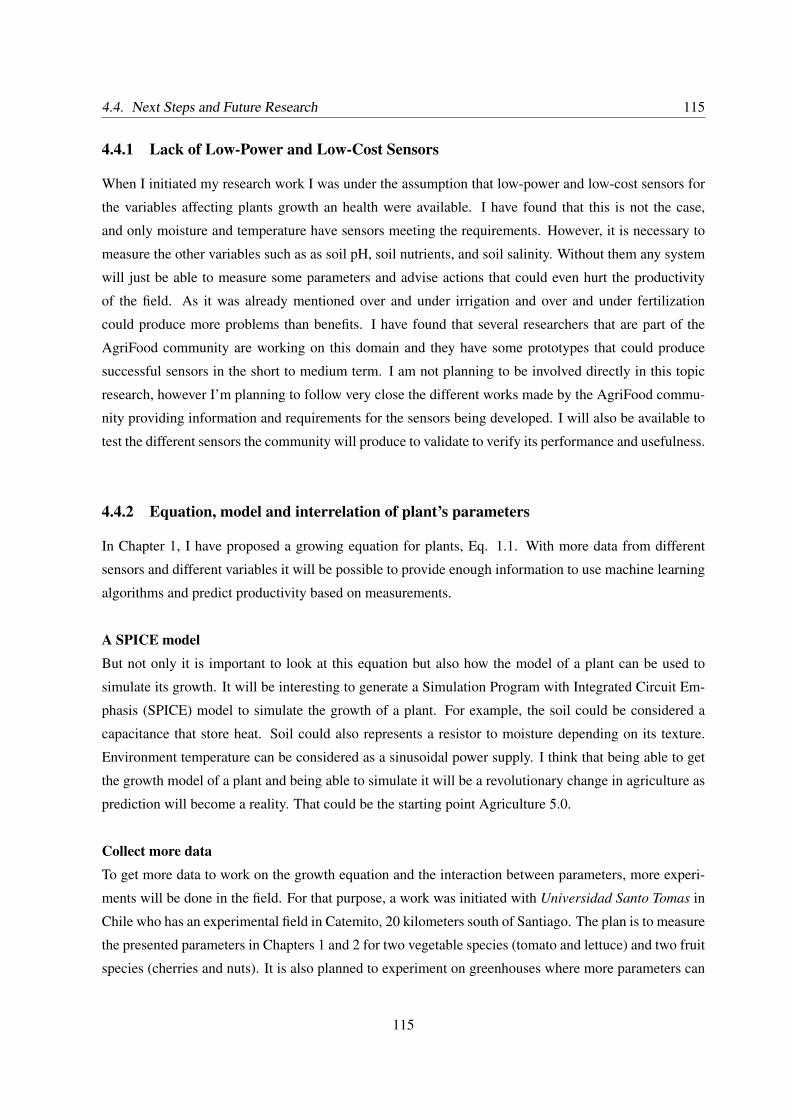
4.4. Next Steps and Future Research 115
4.4.1 Lack of Low-Power and Low-Cost Sensors
When I initiated my research work I was under the assumption that low-power and low-cost sensors for
the variables affecting plants growth an health were available. I have found that this is not the case,
and only moisture and temperature have sensors meeting the requirements. However, it is necessary to
measure the other variables such as as soil pH, soil nutrients, and soil salinity. Without them any system
will just be able to measure some parameters and advise actions that could even hurt the productivity
of the field. As it was already mentioned over and under irrigation and over and under fertilization
could produce more problems than benefits. I have found that several researchers that are part of the
AgriFood community are working on this domain and they have some prototypes that could produce
successful sensors in the short to medium term. I am not planning to be involved directly in this topic
research, however I’m planning to follow very close the different works made by the AgriFood commu-
nity providing information and requirements for the sensors being developed. I will also be available to
test the different sensors the community will produce to validate to verify its performance and usefulness.
4.4.2 Equation, model and interrelation of plant’s parameters
In Chapter 1, I have proposed a growing equation for plants, Eq. 1.1. With more data from different
sensors and different variables it will be possible to provide enough information to use machine learning
algorithms and predict productivity based on measurements.
A SPICE modelBut not only it is important to look at this equation but also how the model of a plant can be used to
simulate its growth. It will be interesting to generate a Simulation Program with Integrated Circuit Em-
phasis (SPICE) model to simulate the growth of a plant. For example, the soil could be considered a
capacitance that store heat. Soil could also represents a resistor to moisture depending on its texture.
Environment temperature can be considered as a sinusoidal power supply. I think that being able to get
the growth model of a plant and being able to simulate it will be a revolutionary change in agriculture as
prediction will become a reality. That could be the starting point Agriculture 5.0.
Collect more dataTo get more data to work on the growth equation and the interaction between parameters, more experi-
ments will be done in the field. For that purpose, a work was initiated with Universidad Santo Tomas in
Chile who has an experimental field in Catemito, 20 kilometers south of Santiago. The plan is to measure
the presented parameters in Chapters 1 and 2 for two vegetable species (tomato and lettuce) and two fruit
species (cherries and nuts). It is also planned to experiment on greenhouses where more parameters can
115
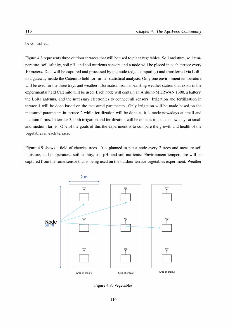
116 Chapter 4. The AgriFood Community
be controlled.
Figure 4.8 represents three outdoor terraces that will be used to plant vegetables. Soil moisture, soil tem-
perature, soil salinity, soil pH, and soil nutrients sensors and a node will be placed in each terrace every
10 meters. Data will be captured and processed by the node (edge computing) and transferred via LoRa
to a gateway inside the Catemito field for further statistical analysis. Only one environment temperature
will be used for the three trays and weather information from an existing weather station that exists in the
experimental field Catemito will be used. Each node will contain an Arduino MKRWAN 1300, a battery,
the LoRa antenna, and the necessary electronics to connect all sensors. Irrigation and fertilization in
terrace 1 will be done based on the measured parameters. Only irrigation will be made based on the
measured parameters in terrace 2 while fertilization will be done as it is made nowadays at small and
medium farms. In terrace 3, both irrigation and fertilization will be done as it is made nowadays at small
and medium farms. One of the goals of this the experiment is to compare the growth and health of the
vegetables in each terrace.
Figure 4.9 shows a field of cherries trees. It is planned to put a node every 2 trees and measure soil
moisture, soil temperature, soil salinity, soil pH, and soil nutrients. Environment temperature will be
captured from the same sensor that is being used on the outdoor terrace vegetables experiment. Weather
Figure 4.8: Vegetables
116

4.4. Next Steps and Future Research 117
information will come from the existing weather station. Data will be processed locally and transferred
through LoRa to a gateway and will be studied to see how the parameters evolve on a cherry produc-
tion. A similar experiment will be conducted with nuts as shown in Figure 4.10. The objective of this
experiment is also to see how measurements can help to improve productivity.
Figure 4.9: Cherries
Figure 4.10: Nuts
117
118 Chapter 4. The AgriFood Community
Experiments on a greenhouseFinally, experiments will be done on a greenhouse as depicted in Figure 4.11 with two trays using let-
tuces. The analysis of how others parameters behave and what are their influence on plant growth and
health thanks to their artificial modification. The expected outcome of those experiments are:
• Verification of the growth function presented previously,
• Definition of parameters weight,
• Find out the optimum measurement periodicity for each parameter per species,
• Find out the optimum distance between sensors,
• Analyze and model the interaction between parameters.
For the purpose of this work, and to be able to execute the experiments, high-cost and even high-power
sensors will be used. I am planning to be fully involved in these experiments and on the conclusions the
experiments will provide.
4.4.3 Better understanding of plants growth for better IoT systems
Understanding plants and its behavior is critical to understand their growth and being able to control
it. I have presented the topic in the first and second chapter of this thesis. However more work is still
Figure 4.11: Greenhouse
118
4.4. Next Steps and Future Research 119
necessary. With this knowledge, values coming from sensors can be better handled by IoT systems. For
example, the amount of water consumed by plants is different depending on the species and the devel-
opment stage of the plant. I have not found any system that is customized at that level of detail. Other
important variables such as soil texture are not considered by any system I have found. The amount of
water and the periodicity of irrigation also depends on the type of soil. Adding this kind of knowledge
to an IoT system for agriculture is what will make the difference between what exist today and what is
needed. I know that several researchers of the AgriFood community are also analyzing this topic and
proposing some ideas into their specific domain, e.g. sensors. It is necessary to continue developing our
knowledge and its applications to the future systems that will be developed. I’m planning to be fully
involved in this topic.
Sensor accuracy over time Sensors used by the IoT system are intended to be placed in the field and
they should work for longtime without any human intervention. For an ADMS IoT system as the one
presented in this manuscript, a three years duration without human intervention is considered reasonable.
So, it is important to verify the service life of the sensors that will be used. Experiments have to be made
to verify the accuracy of sensors over time, for that purpose a methodology to simulate the time (3 years)
have to be find and used with all the selected sensors. I am not planning to be fully involved in this topic,
however I will contribute with my measurements and comments to the people working on the sensors in
the AgriFood community.
Other parameters not yet consideredThis work have analyzed and considered some parameters affecting plant growth and health. The con-
sidered parameters are mostly soil parameters as it is clearly detailed in Chapter 1. However other
parameters can also influence the growth and health of plants, such as pests, insects, and birds among
others. Lettuce beds are planted when they have their first two leaves, but many of them are eaten by
birds as it shown in Figure 4.12. Farmers use ancestral knowledge to scare the birds, having a good suc-
cess rate, but measuring the presence of birds and automatically activating some form of bird repellent
will improve soil productivity. Other environment parameters and phenomena such as wing and frost
should also be considered. For example wind increases the evotranspiration, so the plant needs more
water. Using current wind speed and predictions from weather stations will also help to improve the
productivity of the soil and the quantity of water used for irrigation. Frost when fruit trees are in bloom
causes freezing of the blossom and loss of fruit. A warning to farmers indicating the situation will allow
them to take some actions and avoids the lose of production.
Being close to farmers will provide a lot of information and insights of parameters to be measured and
119
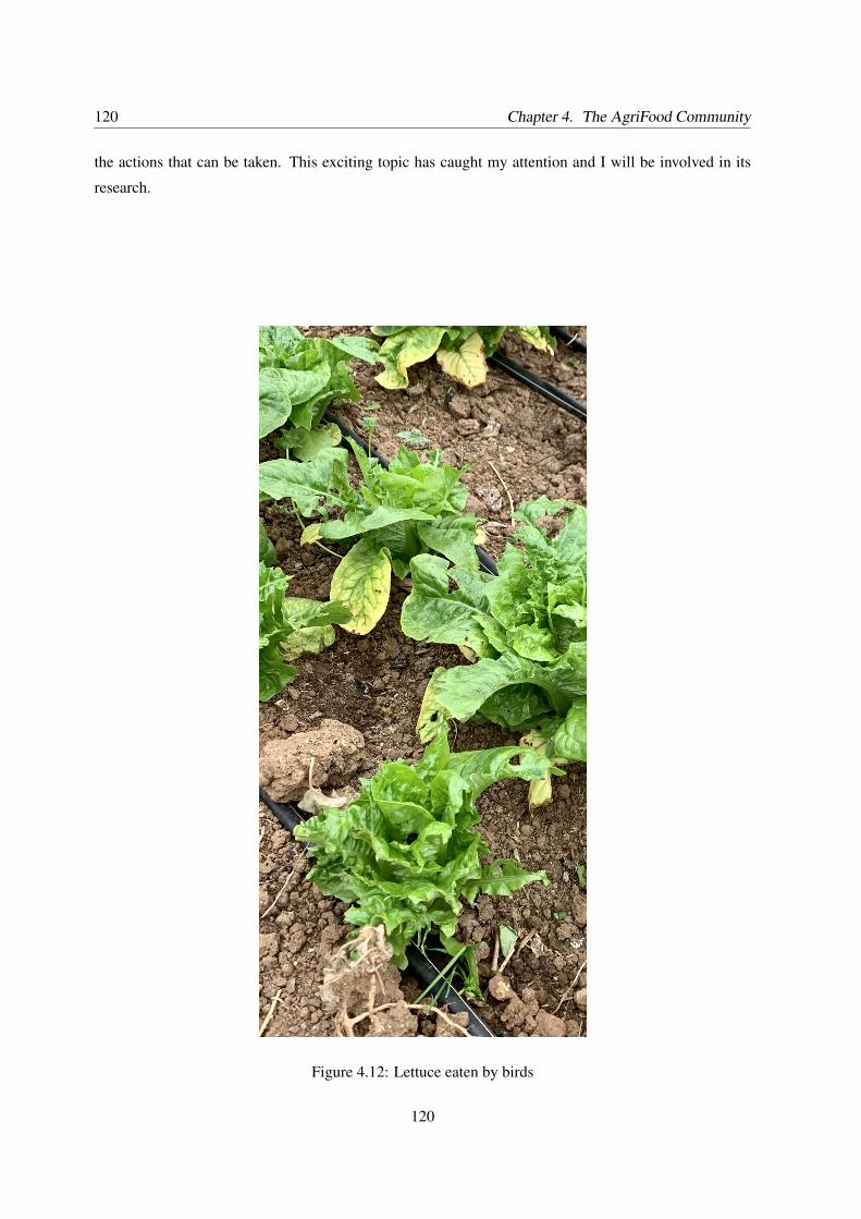
120 Chapter 4. The AgriFood Community
the actions that can be taken. This exciting topic has caught my attention and I will be involved in its
research.
Figure 4.12: Lettuce eaten by birds
120
4.5. Conclusion 121
4.4.4 Enhance capabilities of the SoC
The communication technology chosen for the IoT system cannot be integrated into the SoC I have
designed. I am planning to continue my research on this topic and find a way, even using another compa-
rable communication technology, to integrate the communication into the SoC decreasing the total area
and the power of the system.
Fabrication and characterization of the SoCI have stated in this document that to accomplish the requirements of the low-cost and low-power system
a dedicated SoC designed for smart agriculture applications is essential. I have worked on the design of
the SoC. I have presented the layout of the chip as part of this work. However it is necessary to continue
in this path and fabricate the chip. So the proposed IoT system is prepared and tested in the field. That
implies that all necessary steps form the final layout generation to the produced and working chip are
done. The deployment of the system on small and medium farmers is the step that could conclude this
work.
I have just started a project with Universidad de la Frontera, Temuco, Chile, who are interested in this
SoC for an IoT system dedicated to the dairy industry. I will work with them to conclude the design and
the manufacturing of the chip.
Deployment of the IoT systemIt is important to build the edge of the proposed IoT system including the communication technology,
Lora. Necessary actuators should be defined and implemented. Also, the edge should be able to transmit
data to a server in the cloud once a day for further analysis. I’m also planning to be involved on this
continuation of the work.
4.5 Conclusion
Smart agriculture and Agriculture 4.0 are terms that consider the usage of technology on the agriculture.
Several researchers and companies around the world are working on this domain as it is so important for
the preservation of the humanity. It is necessary to feed more people in the next 30 years and it is also
necessary to get that necessary food without impacting the planet and its environment. An important
community exists and is growing through collaboration between its members. This community has to
face several challenges and they are all urgent and need to be solved as soon as possible. I have concen-
trated my research on plants that grow in the soil, and I have detailed how they grow and the parameters
121
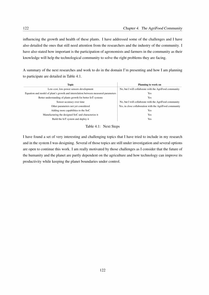
122 Chapter 4. The AgriFood Community
influencing the growth and health of these plants. I have addressed some of the challenges and I have
also detailed the ones that still need attention from the researchers and the industry of the community. I
have also stated how important is the participation of agronomists and farmers in the community as their
knowledge will help the technological community to solve the right problems they are facing.
A summary of the next researches and work to do in the domain I’m presenting and how I am planning
to participate are detailed in Table 4.1.
Topic Planning to work on
Low-cost, low-power sensors development No, but I will collaborate with the AgriFood community
Equation and model of plant’s growth and interrelation between measured parameters Yes
Better understanding of plants growth for better IoT systems Yes
Sensor accuracy over time No, but I will collaborate with the AgriFood community
Other parameters not yet considered Yes, in close collaboration with the AgriFood community
Adding more capabilities to the SoC Yes
Manufacturing the designed SoC and characterize it Yes
Build the IoT system and deploy it Yes
Table 4.1: Next Steps
I have found a set of very interesting and challenging topics that I have tried to include in my research
and in the system I was designing. Several of those topics are still under investigation and several options
are open to continue this work. I am really motivated by those challenges as I consider that the future of
the humanity and the planet are partly dependent on the agriculture and how technology can improve its
productivity while keeping the planet boundaries under control.
122
Conclusion
When I started this research work considering the problem about productivity and irrigation of plants,
that I had in my own field, especially vegetables. I had in mind that the use of technology was the right
approach to solve the issue I was having. I was also assuming that farmers, especially small and medium,
were facing a similar problem. Then, I started to look at what was being done around the world and I
found that the problem I was seeing in my field was a bigger issue and it was happening worldwide.
Continuing with my research, I found that very few solutions considering plant’s growth were developed
at that time, and I also found that an important part of the research in this domain were done in countries
were agriculture played an important role in their economies. Firstly, I thought that a general solution,
was not the right approach and a specific solution for agriculture were to be designed. This idea guided
all my research work.
I started to study how a plant growth and how to take care of the health of plants and I have presented
what I have learnt and formalized in Chapter 1. It is possible then to conclude that a plant is a com-
plex living system and its growth depends on several physical and chemical parameters that I presented
in the chapter. Looking for a mathematical model that includes all the presented parameters will en-
able to predict in some way the growth and therefore the productivity of a field. Another conclusion of
this study of plants is that different species have different requirements. A unique IoT system is not pos-
sible, and IoT systems have to be customized based on the species and the environment they will operate.
I have also found that agriculture as it is done nowadays is impacting negatively the planet boundaries
and the global warming. A big dilemma has to be solved if productivity of the soil has to be increased.
The question there is how to increase soil productivity while keeping the planet safe? I considered that
technology could be a direction to solve the dilemma and will allow farmers to increase the yield of their
land without impacting the planet.
In Chapter 2, I studied how to measure the parameters I considered important to monitor and control the
growth and health of plants, having in mind small and medium farmers. For them, the cost of an IoT
system is important and my research was oriented to low-cost sensors or systems to measure the defined
123
124 Chapter 4. The AgriFood Community
parameters. I have found that low-cost sensors exist only for some of the necessary parameters used to
monitor and control the growth and health of a plant. A second conclusion is that low-cost sensors are
necessary to implement any technological solution in small and medium farms. But not only low-cost is
needed for the sensors and the IoT system considered as part of this research work. Low-power is also
important as the system has to work for several years, without any human intervention. So the requested
sensors have to be together low-power and low-cost.
With all this knowledge in mind, I designed in Chapter 3 a SoC and an IoT system based on the SoC
meeting the following requirements: low-cost, low-power, easy-to-use, in-situ, and real-time. With this
system, a new way of doing agriculture can be considered. The SoC has been designed with satisfactory
results. The power consumed by the SoC and by the system are low. A 10.000 mAH battery the system
can last up to 3 years without human intervention. Regarding low-cost, only sensors for soil temperature
and soil humidity have been found meeting the system requirements, so a lot of work is still to be done
in this domain to be able to build a useful system for small and medium farmers.
I have found an interesting community working on different topics related to agriculture and technology.
This community gave me a lot of knowledge that was the basis for my own research and the SoC and
IoT system I have designed. I contributed a lot to the community and I am still actively collaborating as
I think that by joining the efforts of several researchers, the improvement of agriculture through technol-
ogy will be possible. Not only it is necessary to increase the yield of the soil but it is mandatory to do it
keeping in mind that the salvation of the planet is in our hands.
I have demonstrated that technology should be the driver for a new way to do agriculture and produce
food. I have also explained that a specific system is necessary if the productivity has to be increased
while keeping the planetary boundaries under control and at levels where there is no major risk for the
planet. The system I am considering and I have designed is an IoT edge based on a SoC. The system is
flexible and can be connected to different kind of sensors and actuators, and send data to the cloud as
well. The system can also be customized based on species and environment.
The work is still in progress as it is shown in Chapter 4. Several topics need further investigation and
development. Sensors to be created, modelling the growth of a plant, study the interaction between
physical and chemical parameters influencing the growth of a plant, adding additional parameters to be
measured, manufacturing the SoC and the IoT system are some of the next steps I propose and consider
to do. The achievement of those steps will allow small and medium farmers to use the technology to
improve their productivity while keeping the planet safe.
124
Publications
Journals
[ J1 ] V. Grimblatt, C. Jégo, G. Ferré and F. Rivet, "How to Feed a Growing population - An IoT
Approach to Crop Health and Growth," in IEEE Journal on Emerging and Selected Topics in
Circuits and Systems (JETCAS), doi: 10.1109/JETCAS.2021.3099778.
International Conferences
[ C1 ] V. Grimblatt, G. Ferré, F. Rivet, C. Jego and N. Vergara, "Precision AgriPrecision Agriculture -
Improving The Soil Yield Using Internet of Things," ICECS 2018, 2018
[ C2 ] V. Grimblatt, G. Ferré, F. Rivet, C. Jego and N. Vergara, "Precision Agriculture for Small to
Medium Size Farmers — An IoT Approach," 2019 IEEE International Symposium on Circuits
and Systems (ISCAS), 2019, pp. 1-5, doi: 10.1109/ISCAS.2019.8702563.
[ C3 ] V. Grimblatt, "IoT for Agribusiness: An overview," 2020 IEEE 11th Latin American Symposium
on Circuits and Systems (LASCAS), 2020, pp. 1-4, doi: 10.1109/LASCAS45839.2020.9068986.
[ C4 ] V. Grimblatt, "The Challenge of Agriculture: Increase the Productivity in a Sustainable Way"
Forum on Specification and Design Languages, FDL 2021, September 2021.
Books
[ B1 ] V. Grimblatt, "Technology and Agribusiness: How Technology is Impacting Agribusiness" River
Publishers, August 2021, ISBN 9788770225977
Talks
[ T1 ] V. Grimblatt, "Smart Agriculture - How To Improve the Throughput of the Soil using IoT?"
Multicore and multiprocessor SoC (MPSoC) 2018, http://www.mpsoc-forum.org/speakers/
page/Victor_Grimblatt.html
125
126 Chapter 4. The AgriFood Community
[ T2 ] V. Grimblatt, "IoT for Agronomists - An Introduction" Universidad Santo Tomas, Santiago,
Chile, April 2019
[ T3 ] V. Grimblatt. C. Jego, G. Ferré, F. R ivet, "A SoC for IoT Applied to Smart Agriculture" Multicore
and multiprocessor SoC (MPSoC) 2019, , http://www.mpsoc-forum.org/speakers/
page/Victor_Grimblatt.html
[ T4 ] V. Grimblatt, "Tecnologías en la industria 4.0 y su uso en el sector agrícola. Experiencias a nivel
mundial" Aplicación de las Tecnologías de la Industria 4.0 en el Sector Agrícola, November 20,
2019, https://www.virtualpro.co\/eventos\/aplicacion-de-las-tecnologias-de-la-industria-4-0-en-el-sector-agricola
[ T5 ] V. Grimblatt, "The Application of Technology in the Agribusiness" Escola Sul de Microeletrônica
(EMicro 2020), April 30, 2020, https://www.youtube.com/watch?v=RQJgEBDaHWI
[ T6 ] V. Grimblatt, "Agribusiness and technology - an Overview" FoodCAS 2020, October 22, 2020,
[ T7 ] V. Grimblatt, "To Drink or to Die, that is the question. When IoT can save us before getting
thirsty . . . and hungry." Bordeaux IEEE Bee, December 4, 2020,
[ T8 ] V. Grimblatt, "How to feed a growing population while conserving the planet’s resources – IoT
to the Rescue" IEEE IoT Webinar, August 11, 2021,
Courses
[ Co1 ] IoT for Agronomist, October - November 2020
[ Co2 ] "Improving the Productivity of the Soil – An IoT Approach", 1st IEEE CAS Seasonal School
Technology and Agribusiness: How the Technology is Impacting the Agribusiness November 2020
126
Bibliography
[1] J. Lokrantz/Azote based on Steffen et al. Planetary Boundaries. https://www.
stockholmresilience.org/research/planetary-boundaries.html, 2015.
[2] Kate Raworth. Doughnut Economics: Seven Ways to Think Like a 21st-Century Economist. Chelsea
Green Publishing, 2017.
[3] The World Bank. World Bank. https://data.worldbank.org/.
[4] Sarah K. Lowder, Jakob Skoet, and Terri Raney. The number, size, and distribution of farms,
smallholder farms, and family farms worldwide. World Development, 87:16–29, November 2016.
[5] Our World in Data. Land Use. https://ourworldindata.org/land-use.
[6] ameliamurtha. Soil Texture Pyramid. https://ameliamurtha.wordpress.com/2016/02/28/
the-soil-texture-pyramid/.
[7] Susie Roques, Sarah Kendall, K.A. Smith, Paul Newell Price, and P. Berry. Review of the non-npks
nutrient requirements of uk cereals and oilseed rape. 2013.
[8] Knud Lasse Lueth. Why the Internet of Things is called Internet of Things: Definition, history,
disambiguation. https://iot-analytics.com/internet-of-things-definition/#:~:
text=A%20brief%20history%20of%20the%20Internet%20of%20Things&text=But%20the%
20actual%20term%20%E2%80%9CInternet,new%20exciting%20technology%20called%
20RFID.
[9] Daniel Nenni and Mitch Heins. Custom SoCs for IoT: Simplified. SCRIBD, 2018.
[10] Sophocleous Marios and Julius Georgiou. Precision agriculture: Challenges in sensors and elec-
tronics for real-time soil and plant monitoring. In 2017 IEEE Biomedical Circuits and Systems
Conference (BioCAS), pages 1–4, 2017.
[11] Rui-Tao Liu, Lu-Qi Tao, Bo Liu, Xiang-Guang Tian, Mohammad Mohammad, Yi Yang, and Tian-
ling Ren. A miniaturized on-chip colorimeter for detecting npk elements. Sensors, 16:1234, 08
2016.
127
128 Bibliography
[12] Lab Grade ph Probe. https://atlas-scientific.com/ph-probe.
[13] Almaw Aniley, Naveen Kumar, and Akshaya Kumar. Soil temperature sensors in agriculture and
the role of nanomaterials in temperature sensors preparation. pages 363–372, 01 2017.
[14] DS18B20. https://www.maximintegrated.com/en/products/sensors/DS18B20.html#
tech-docs.
[15] Principles of regenerative agriculture. https://ourgoodbrands.com/
what-is-regenerative-agriculture-why-matters/.
[16] United Nations sustainable development goals. https://sdgs.un.org/goals.
[17] Susan Parent. How Does Humidity Influence Crop Quality? https://www.pthorticulture.
com/en/training-center/how-does-humidity-influence-crop-quality/.
[18] Water Footprint Network. Water Stress. https://waterfootprint.org/en/about-us/news/
news/water-stress-affect-52-worlds-population-2050/.
[19] United Nations. United Nations SDGS. https://sdgs.un.org/.
[20] Shenggen Fan and Christopher Rue. Role of Smallholder Farms in a Changing World, pages 13–28.
Springer International Publishing, 2020.
[21] John Carlo Puno, Edwin Sybingco, Elmer Dadios, Ira Valenzuela, and Joel Cuello. Determination
of soil nutrients and ph level using image processing and artificial neural network. In 9th Inter-
national Conference on Humanoid, Nanotechnology, Information Technology, Communication and
Control, Environment, and Management (HNICEM ), 2017.
[22] M. Onwuka. Effects of soil temperature on some soil properties and plant growth. Adv. Plants
Agric, Res 8, 2018.
[23] Pooja Shrivastava and Rajesh Kumar. Soil salinity: A serious environmental issue and plant growth
promoting bacteria as one of the tools for its alleviation. Saudi Journal of Biological Sciences,
22(2):123–131, 2015.
[24] Rui Manuel Almeida Machado and Ricardo Paulo Serralheiro. Soil salinity: Effect on vegetable
crop growth. management practices to prevent and mitigate soil salinization. Horticulturae, 3(2),
2017.
[25] Shabbir A. Shahid, Mohammad Zaman, and Lee Heng. Soil Salinity: Historical Perspectives and
a World Overview of the Problem, pages 43–53. Springer International Publishing, Cham, 2018.
128
Bibliography 129
[26] Charles Darwin. The Power of Movement in Plants. Cambridge Library Collection - Darwin,
Evolution and Genetics. Cambridge University Press, 2009.
[27] Jose Chen Lopez. Influence of Light on Crop Growth. https://www.pthorticulture.com/en/
training-center/influence-of-light-on-crop-growth/.
[28] Jerry L. Hatfield and John H. Prueger. Temperature extremes: Effect on plant growth and develop-
ment. Weather and Climate Extremes, 10:4–10, 2015. USDA Research and Programs on Extreme
Events.
[29] K.M. Barlow, B.P. Christy, G.J. O’Leary, P.A. Riffkin, and J.G. Nuttall. Simulating the impact of
extreme heat and frost events on wheat crop production: A review. Field Crops Research, 171:109–
119, 2015.
[30] Polygon. How Humidity Affects the Growth of Plants. https://www.polygongroup.com/en-US/
blog/how-humidity-affects-the-growth-of-plants/#:~:text=Relative%20humidity%
20is%20the%20amount,hold%20at%20a%20certain%20temperature.&text=When%
20surrounded%20by%20warm%20temperatures,a%20grower%20to%20fertilize%20it.
[31] Alexander S. Gillis. Internet of Things - IoT. =
https://internetofthingsagenda.techtarget.com/definition/Internet-of-Things-IoT.
[32] Maciej Kranz. 7 ways IoT is reshaping the internet. https://www.networkworld.com/article/
3234749/7-ways-iot-is-reshaping-the-internet.html.
[33] Michael E. Porter and James E. Heppelmann. How Smart, Connected Products Are Transforming
Companies. http://bit.ly/1LXG2NM, 2015.
[34] Perry Lea. Internet of Things for Architects. Packt, 2018.
[35] Crystal Bedell. How Edge Computing Technology Is Reshaping
the IoT Landscape. https://www.iotworldtoday.com/2019/12/13/
how-edge-computing-technology-is-reshaping-the-iot-landscape/, 2019.
[36] Thales. Low Power Wide Area Technology. https://www.thalesgroup.com/en/
markets/digital-identity-and-security/iot/resources/innovation-technology/
low-power-wide-area-technology.
[37] Sharon Shea. Low Power Wide Area Network. https://internetofthingsagenda.
techtarget.com/definition/LPWAN-low-power-wide-area-network.
129
130 Bibliography
[38] Keith Fuglie. Precision Agriculture. https://www.sciencedirect.com/topics/
earth-and-planetary-sciences/precision-agriculture, 2016.
[39] E. Gilad, J. von Hardenberg, A. Provenzale, M. Shachak, and E. Meron. A mathematical model of
plants as ecosystem engineers. Journal of Theoretical Biology, 244(4):680–691, 2007.
[40] Hunt R. Causton and Shipley B. Askew. A modern tool for classical plant growth analysis. Annals
of botany, 90(4):485–488, 2002.
[41] N. Bessonov. Dynamical models of plant growth. 2006.
[42] Thierry Fourcaud, Xiaopeng Zhang, Alexia Stokes, Hans Lambers, and Christian Körner. Plant
Growth Modelling and Applications: The Increasing Importance of Plant Architecture in Growth
Models. Annals of Botany, 101(8):1053–1063, 04 2008.
[43] G.I Metternicht and J.A Zinck. Remote sensing of soil salinity: potentials and constraints. Remote
Sensing of Environment, 85(1):1–20, 2003.
[44] Romit Atta. Farming 2.0: How does IoT help Agriculture domain? https://netmanias.com/
en/post/blog/12735/iot/farming-2-0-how-does-iot-help-agriculture-domain#:
~:text=Apart%20from%20generating%20crop%20and,done%20in%20the%20right%
20amounts., 2017.
[45] Mahammad Shareef Mekala and P. Viswanathan. A novel technology for smart agriculture based
on iot with cloud computing. In 2017 International Conference on I-SMAC (IoT in Social, Mobile,
Analytics and Cloud) (I-SMAC), pages 75–82, 2017.
[46] Sriveni Namani and Bilal Gonen. Smart agriculture based on iot and cloud computing. In 2020
3rd International Conference on Information and Computer Technologies (ICICT), pages 553–556,
2020.
[47] Mohamed Rawidean Mohd Kassim. Iot applications in smart agriculture: Issues and challenges. In
2020 IEEE Conference on Open Systems (ICOS), pages 19–24, 2020.
[48] Amarendra Goap, Deepak Sharma, A.K. Shukla, and C. Rama Krishna. An iot based smart irri-
gation management system using machine learning and open source technologies. Computers and
Electronics in Agriculture, 155:41–49, 2018.
[49] Uélison Jean L. dos Santos, Gustavo Pessin, Cristiano André da Costa, and Rodrigo da Rosa Righi.
Agriprediction: A proactive internet of things model to anticipate problems and improve production
in agricultural crops. Computers and Electronics in Agriculture, 161:202–213, 2019. BigData and
DSS in Agriculture.
130
Bibliography 131
[50] GSMA. COVID-19: Accelerating the Use of Digital Agricul-
ture. https://www.gsma.com/mobilefordevelopment/resources/
covid-19-accelerating-the-use-of-digital-agriculture/, 2021.
[51] Jitendra Patidar, Rajesh Khatri, and R.C. Gurjar. Precision agriculture system using verilog hard-
ware description language to design an asic. In 2019 3rd International Conference on Electronics,
Materials Engineering Nano-Technology (IEMENTech), 2019.
[52] B. Moses Madhukar and V. Padmanabha Reddy. Design and development of fpga based wireless
soc for precision agriculture. European Journal of Molecular & Clinical Medicine, 8(1):1687–
1706, 2021.
[53] Robert Bogue. Sensors key to advances in precision agriculture. Sensor Review, 37:1–6, 01 2017.
[54] Anchit Garg, Priyamitra Munoth, and Rohit Goyal. Application of soil moisture sensors in agricul-
ture: A review. 12 2016.
[55] Fedro S. Zazueta and Jiannong Xin. Soil moisture sensors. Bulletin 292, Florida Cooperative
Extension Service, Institute of Food and Agricultural Sciences, University of Florida, 04 1994.
[56] FC28. https://components101.com/modules/soil-moisture-sensor-module.
[57] SEN0193. https://media.digikey.com/pdf/Data%20Sheets/DFRobot%20PDFs/SEN0193_
Web.pdf.
[58] Hak-Jin Kim, Kenneth A. Sudduth, and John W. Hummel. Soil macronutrient sensing for precision
agriculture. J. Environ. Monit., 11:1810–1824, 2009.
[59] Marianah Masrie, Mohamad Syamim Aizuddin Rosman, Rosidah Sam, and Zuriati Janin. Detec-
tion of nitrogen, phosphorus, and potassium (npk) nutrients of soil using optical transducer. In
2017 IEEE 4th International Conference on Smart Instrumentation, Measurement and Application
(ICSIMA), 2017.
[60] Deepa Ramane, Supriya Patil, and A. Shaligram. Detection of npk nutrients of soil using fiber optic
sensor. 02 2015.
[61] LAQUA. Ways of Measuring pH. https://www.horiba.
com/es/application/material-property-characterization/
water-analysis/water-quality-electrochemistry-instrumentation/
the-story-of-ph-and-water-quality/the-story-of-ph/ways-of-measuring-ph/.
131
132 Bibliography
[62] Victorian Resources Online. Measuring and Interpreting Soil pH. http://vro.agriculture.
vic.gov.au/dpi/vro/vrosite.nsf/pages/soilhealth_measure_ph.
[63] Michael Schirrmann, Robin Gebbers, Eckart Kramer, and Jan Seidel. Soil ph mapping with an
on-the-go sensor. Sensors, 11(1):573–598, 2011.
[64] Luke Scheberl, Bryant C. Scharenbroch, Les P. Werner, Jacob R. Prater, and Kelby L. Fite. Evalua-
tion of soil ph and soil moisture with different field sensors: Case study urban soil. Urban Forestry
& Urban Greening, 38:267–279, 2019.
[65] Dennis Corwin. Soil Salinity Measurement, pages 852–857. 01 2003.
[66] Julien Roux, Jean-Yves Fourniols, Georges Soto-Romero, and Christophe Escriba. A connected
soil humidity and salinity sensor for precision agriculture. In 2018 International Conference on
Computational Science and Computational Intelligence (CSCI), pages 1028–1031, 2018.
[67] ISL29125. https://www.renesas.com/us/en/document/dst/isl29125-datasheet.
[68] GY-302 BH1750. http://wiki.sunfounder.cc/index.php?title=GY-302_BH1750_
Digital_Light_Intensity_Module.
[69] Hardware/Software Co-Design. Springer Netherlands, 1996.
[70] DesignWare ARC EM Starter Kit. https://www.synopsys.com/dw/ipdir.php?ds=arc_em_
starter_kit.
[71] I2C Humidity and temperature Sensor. https://www.silabs.com/documents/public/
data-sheets/Si7021-A20.pdf.
[72] Synopsys. Building an Efficient, Tightly Coupled Embedded Sys-
tem Using an Extensible Processor. https://semiengineering.com/
building-an-efficient-tightly-coupled-embedded-system-using-an-extensible-processor/.
[73] DesignWare® ARC® Synopsys ASIC Reference Design Flow User’s Guide. =
https://www.synopsys.com/dw/doc.php/iip/dwc_arc_vpx5x2_dsp/latest/doc/ARC_Synopsys_ASIC_RDF_User_Guide.pdf.
[74] DesignWare® ARChitect User’s Guide. https://spdocs.synopsys.com/dow_retrieve/
O-2018.09/arc/architect/ARChitect_UserGuide/cover.pdf.
[75] ARC EM4. https://www.synopsys.com/dw/ipdir.php?ds=arc-em4-em6.
[76] DesignWare ARC EM Databook. https://www.synopsys.com/dw/doc.php/iip/DWC_ARC_EM/
5.10a/ARC_EM_Databook.pdf.
132
Bibliography 133
[77] Designware ARC Sensor and Control IP Subsystem Databook. https://www.synopsys.com/
dw/doc.php/iip/dwc_sensor_subsystem/latest/doc/SensorControlSubsystem_CTRL_
Databook.pdf.
[78] Food Security. https://www.ifpri.org/topic/food-security.
[79] Regenerative Agriculture. https://www.greenamerica.org/healthy-soil-cool-climate/
regenerative-agriculture-101.
[80] Regeneration International. https://regenerationinternational.org/
why-regenerative-agriculture/.
133

134 Bibliography
134
APPENDIX
AAPPENDIX A
SommaireA.1 Nutrients . . . . . . . . . . . . . . . . . . . . . . . . . . . . . . . . . . . . . . . . . 136
A.1.1 Macronutrients . . . . . . . . . . . . . . . . . . . . . . . . . . . . . . . . . . 136
A.1.2 Micronutrients . . . . . . . . . . . . . . . . . . . . . . . . . . . . . . . . . . 137
A.2 Soil Temperature . . . . . . . . . . . . . . . . . . . . . . . . . . . . . . . . . . . . . 139
A.2.1 Amount of Heat Supplied at the Surface . . . . . . . . . . . . . . . . . . . . . 139
A.2.2 Amount of Heat Dissipated from the Surface . . . . . . . . . . . . . . . . . . 139
A.2.3 Soil Temperature Effects . . . . . . . . . . . . . . . . . . . . . . . . . . . . . 139
A.3 Light . . . . . . . . . . . . . . . . . . . . . . . . . . . . . . . . . . . . . . . . . . . 140
A.3.1 Light Quantity . . . . . . . . . . . . . . . . . . . . . . . . . . . . . . . . . . 140
A.3.2 Light Quality . . . . . . . . . . . . . . . . . . . . . . . . . . . . . . . . . . . 141
A.3.3 Light Duration . . . . . . . . . . . . . . . . . . . . . . . . . . . . . . . . . . 142
135
136 Appendix A. Appendix A
A.1 Nutrients
A.1.1 Macronutrients
Nitrogen (N)
• Part of all living cells and is necessary to all proteins, enzymes and metabolic processes involved
in the synthesis and transfer of energy,
• Part of chlorophyll, green pigment responsible of photosynthesis,
• Helps with rapid growth, increasing seed and fruit production, and improving the quality of leaf
and forage crops,
• Comes from fertilizer application and from the air, water or rainfall contributes very little nitrogen.
Phosphorous (P)
• Essential part of the photosynthesis,
• Involved in the formation of all oils, sugars, and starches,
• Helps with transformation of solar energy into chemical energy,
• Effects rapid growth,
• Encourages blooming and root growth,
• Comes from fertilizer, bone meal, and superphosphate.
Potassium (K)
• Absorbed by plants in larger amount than any other mineral element except nitrogen,
• Helps in the building of proteins, photosynthesis, fruit quality, and reduction of diseases,
• Supplied by soil minerals, organic materials, and fertilizer.
Calcium - Ca
136
A.1. Nutrients 137
• Essential part of the cell wall structure,
• Provides for normal transport and retention of other elements,
• Provides for strength in the plant,
• Helps activate plant enzymes needed for growth,
• Comes from soil minerals, organic materials, fertilizers, and dolomitic limestone.
Magnesium (Mg)
• Part of the chlorophyll,
• Essential for photosynthesis,
• Helps activate enzymes needed for growth,
• Comes from soil mineral, organic material, fertilizers, and dolomitic limestone.
Sulfur (S)
• Essential for protein production,
• Promotes activity and development of enzymes and vitamins,
• Helps in chlorophyll formation,
• Improves root growth and seed production,
• Help with vigorous plant growth and resistance to cold,
• Supplied to the soil from rainwater,
• Added in some fertilizer as an impurity.
A.1.2 Micronutrients
Boron (B)
• Helps in the use of nutrients and regulate other nutrients,
• Aids production of sugar and carbohydrates,
• Essential for seed and fruit development,
• Comes from organic matter and borax.
137
138 Appendix A. Appendix A
Copper (Cu)
• Important for reproductive growth,
• Aids root metabolism,
• Helps in the utilization of proteins.
Chloride (Cl)
• Aids plant metabolism,
• Found in the soil.
Iron (Fe)
• Essential for formation of chlorophyll,
• Sources are soil, iron sulfate, iron chelate.
Manganese (Mn)
• Involved with enzymes in breakdown of carbohydrates and nitrogen metabolism,
• Soil is a source of manganese.
Molybdenum (Mo)
• Helps in the use of nitrogen,
• Soil is a source of molybdenum.
Zinc (Zn)
• Essential for the transformation of carbohydrates,
• Regulates consumption of sugars,
• Part of the enzyme system,
• Sources are soil, zinc oxide, zinc sulfate, zinc chelate.
Micro-nutrients are necessary in reasonable quantities (Boron, Copper, Iron, Chloride, Manganese,
Molybdenum, and Zinc). It is quite complicated to measure all those nutrients, however it is impor-
tant to know how they are important and in some cases which ones have to be measured and controlled.
138
A.2. Soil Temperature 139
A.2 Soil Temperature
A.2.1 Amount of Heat Supplied at the Surface
It depends on several factors:
• Soil color: Dark soils absorb more heat than light color soils,
• Soil mulch: Mulch materials inhibit evaporation and increase soil moisture, in consequence, the
surface serves to insulate heat reducing soil temperature,
• Slope of the land surface: Radiation that reaches the surface at an angle is scattered over a wider
area than the same amount of solar radiation reaching the surface of the land at right angles,
• Vegetative cover: Vegetation is a thermal insulator and affects soil temperature,
• Organic matter content: Organic matter increases the capacity of hold water. It also contributes to
the dark color of the soil. Both properties increase heat’s absorption,
• Evaporation: The greater the rate of evaporation, the more the soil is cooled and temperature
decreases,
• Solar radiation: Corresponds to the amount of heat from the sun that reaches the soil. An increase
of solar radiation increases soil temperature.
A.2.2 Amount of Heat Dissipated from the Surface
It depends on several factors:
• Soil moisture: The flow of heat is higher in a wet soil. The rate of heat dissipation increases with
moisture content,
• Bulk density: High bulk density increases the rate at which heat energy passes through a unit cross
sectional area of the soil.
A.2.3 Soil Temperature Effects
A.2.3.1 Soil Temperature Effect on Biological Soil Properties and Plant Growth
• Bioactivity: Soil temperature between 10°C and 28°C influences soil respiration by
– Increasing the activity of extracellular enzymes that degrade polymeric organic matter,
– Increasing microbial retake of soluble substrates,
139
140 Appendix A. Appendix A
– Increasing microbial respiration,
• Micro-organisms: Require temperatures between 10°C – 35.6°C,
• Macro-organisms: require temperatures between 10°C – 24°C,
• Organic matter decomposition: At temperatures below 0°C the accumulation of soil matter in-
creases due to the slow rate of decomposition. Temperatures between 2°C – 38°C increase organic
matter decomposition.
A.2.3.2 Soil Temperature Effect on Physical Properties
• Soil structure: Increase in temperature produces less clay and more silt-sized particles,
• Aggregate stability: It increases above 30°C,
• Moisture content: Increasing soil temperature decreases water viscosity, allowing more water to
percolate through the soil profile,
• Aeration: High temperature encourages micro-organism activity, increasing the production of car-
bon dioxide.
A.2.3.3 Soil Temperature Effect on Plant Growth
It influences water and nutrient uptake, as well as root and shoot growth.
• Water uptake: Decreases with low temperature, reducing the rate of photosynthesis,
• Nutrient uptake: An increase in soil temperature increases metabolic activities in micro-organisms,
stimulating the availability of nutrients. It has been observed that at low soil temperature, nutrient
uptake is reduced because of high water viscosity and low activity of root nutrient transport,
• Root growth: Increasing soil temperature improves root growth.
A.3 Light
A.3.1 Light Quantity
The rate of the photosynthesis is dependent on the light quantity. Each type of plant starts the photosyn-
thesis at different light energy levels, called the light compensation point. This point starts when light
energy is enough for photosynthetic activity to generate more oxygen than is required by the plant for
respiration. Also, the release of CO2 through plant respiration must be less than the total CO2 used by
the plant for photosynthesis. In other words
140
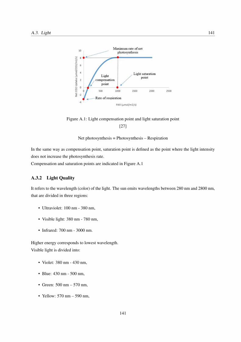
A.3. Light 141
Figure A.1: Light compensation point and light saturation point
[27]
Net photosynthesis = Photosynthesis – Respiration
In the same way as compensation point, saturation point is defined as the point where the light intensity
does not increase the photosynthesis rate.
Compensation and saturation points are indicated in Figure A.1
A.3.2 Light Quality
It refers to the wavelength (color) of the light. The sun emits wavelengths between 280 nm and 2800 nm,
that are divided in three regions:
• Ultraviolet: 100 nm - 380 nm,
• Visible light: 380 nm - 780 nm,
• Infrared: 700 nm - 3000 nm.
Higher energy corresponds to lowest wavelength.
Visible light is divided into:
• Violet: 380 nm - 430 nm,
• Blue: 430 nm - 500 nm,
• Green: 500 nm – 570 nm,
• Yellow: 570 nm – 590 nm,
141
142 Appendix A. Appendix A
• Orange: 590 nm – 630 nm,
• Red: 630 nm – 770 nm.
Photosynthetic Active Radiation (PAR) is defined as the range where plants photosynthesize. This range
is between 400 nm and 700 nm. The chlorophyll in leaves is responsible for absorbing the PAR; it has
two peaks of absorption: blue and red. Different colors have different effects:
• Ultraviolet: Causes DNA damage and reduces photosynthesis rate. Flowering and pollination
decrease. Seed development is also affected. Ultraviolet A can produce plant elongation,
• Blue: It is one of the absorption peaks. It is related to chlorophyll production, so photosynthetic
process is more efficient in the presence of blue light. It is responsible for vegetative and leaf
growth. It is important for seedlings and young plants as it reduces plant stretching,
• Red: The other absorption peak. The photoreceptor phytochrome is more sensitive to and respond
to red light. Regulates flowering and fruiting. It helps to the stem diameter increase and promotes
branching,
• Far red: Causes plant elongation and triggers flowering in long-day plants.
Plants can differentiate between day and night based on the red and far red light. In the morning, red light
is strong, so the plant recognizes that the day begin. In the evening far red light is stronger indicating the
beginning of the night.
Another important factor to consider is the ratio between red light and far red light. A low ratio produces
plant elongation.
A.3.3 Light Duration
Photoperiodism is the response of an organism (plant) to a change in day light. Photoperiodism impacts
flowering. There are 3 categories of plants
• Short-day: Flowers only when the day length is shorter than the night,
• Long-day: Flowers when the day length is longer than the night,
• Day-neutral: Flowers regardless of the day length.
142
APPENDIX
BAPPENDIX B
SommaireB.1 Floorplan . . . . . . . . . . . . . . . . . . . . . . . . . . . . . . . . . . . . . . . . . 144
B.2 SoC Gate Count . . . . . . . . . . . . . . . . . . . . . . . . . . . . . . . . . . . . . 145
B.3 RAM Bits Allocation . . . . . . . . . . . . . . . . . . . . . . . . . . . . . . . . . . . 147
B.4 Core Registers . . . . . . . . . . . . . . . . . . . . . . . . . . . . . . . . . . . . . . 147
B.5 Instructions . . . . . . . . . . . . . . . . . . . . . . . . . . . . . . . . . . . . . . . . 149
B.6 Interrupts . . . . . . . . . . . . . . . . . . . . . . . . . . . . . . . . . . . . . . . . . 153
B.7 PADs . . . . . . . . . . . . . . . . . . . . . . . . . . . . . . . . . . . . . . . . . . . 155
143
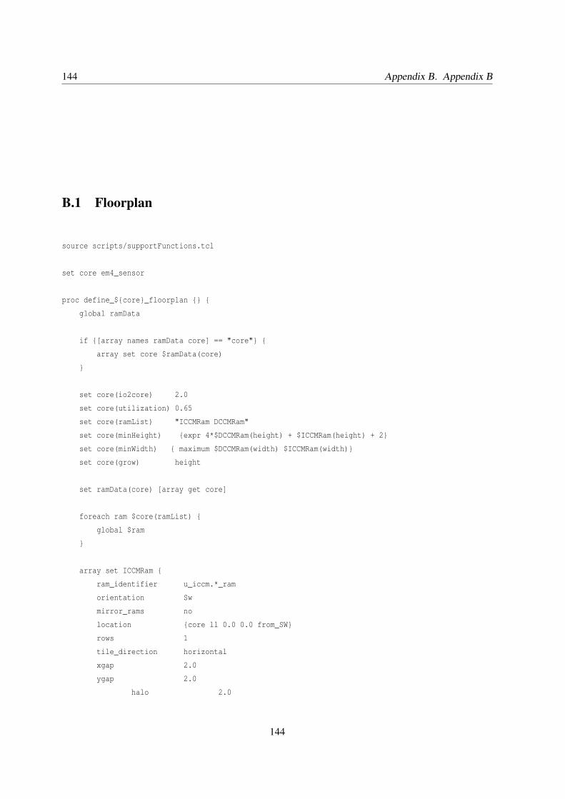
144 Appendix B. Appendix B
B.1 Floorplan
source scripts/supportFunctions.tcl
set core em4_sensor
proc define_${core}_floorplan {} {
global ramData
if {[array names ramData core] == "core"} {
array set core $ramData(core)
}
set core(io2core) 2.0
set core(utilization) 0.65
set core(ramList) "ICCMRam DCCMRam"
set core(minHeight) {expr 4*$DCCMRam(height) + $ICCMRam(height) + 2}
set core(minWidth) { maximum $DCCMRam(width) $ICCMRam(width)}
set core(grow) height
set ramData(core) [array get core]
foreach ram $core(ramList) {
global $ram
}
array set ICCMRam {
ram_identifier u_iccm.*_ram
orientation Sw
mirror_rams no
location {core ll 0.0 0.0 from_SW}
rows 1
tile_direction horizontal
xgap 2.0
ygap 2.0
halo 2.0
144
B.2. SoC Gate Count 145
volt_area CCM
}
array set DCCMRam {
ram_identifier u_dccm_ram
orientation Nw
mirror_rams no
location {core ul 0.0 0.0 from_NW}
rows 1
tile_direction vertical
xgap 2.0
ygap 2.0
halo 2.0
volt_area CCM
}
foreach ram $core(ramList) {
set ramData($ram) [array get $ram]
}
}
define_${core}_floorplan
B.2 SoC Gate Count
Table B.1 presents the gate count for the block of the SoC.
145
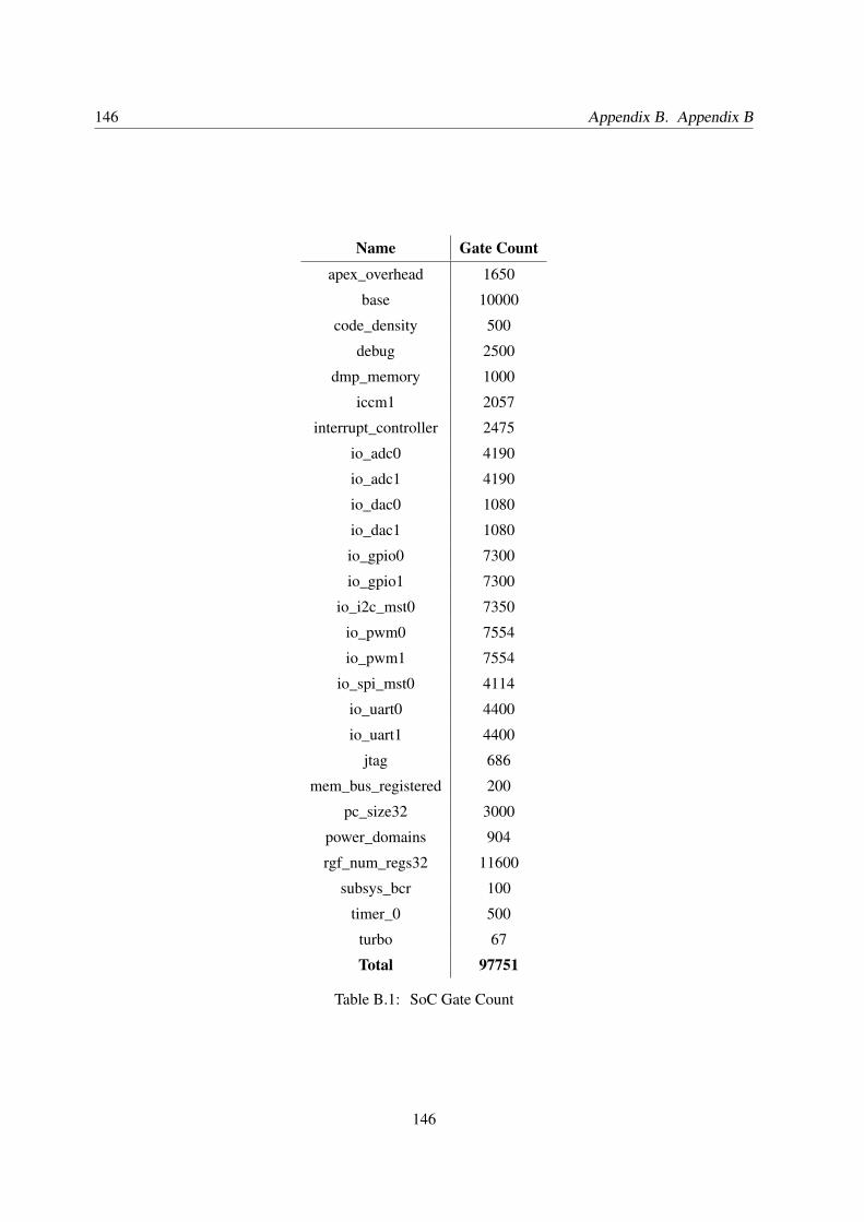
146 Appendix B. Appendix B
Name Gate Count
apex_overhead 1650
base 10000
code_density 500
debug 2500
dmp_memory 1000
iccm1 2057
interrupt_controller 2475
io_adc0 4190
io_adc1 4190
io_dac0 1080
io_dac1 1080
io_gpio0 7300
io_gpio1 7300
io_i2c_mst0 7350
io_pwm0 7554
io_pwm1 7554
io_spi_mst0 4114
io_uart0 4400
io_uart1 4400
jtag 686
mem_bus_registered 200
pc_size32 3000
power_domains 904
rgf_num_regs32 11600
subsys_bcr 100
timer_0 500
turbo 67
Total 97751
Table B.1: SoC Gate Count
146
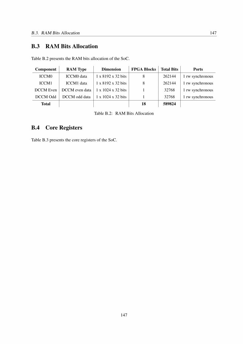
B.3. RAM Bits Allocation 147
B.3 RAM Bits Allocation
Table B.2 presents the RAM bits allocation of the SoC.
Component RAM Type Dimension FPGA Blocks Total Bits Ports
ICCM0 ICCM0 data 1 x 8192 x 32 bits 8 262144 1 rw synchronous
ICCM1 ICCM1 data 1 x 8192 x 32 bits 8 262144 1 rw synchronous
DCCM Even DCCM even data 1 x 1024 x 32 bits 1 32768 1 rw synchronous
DCCM Odd DCCM odd data 1 x 1024 x 32 bits 1 32768 1 rw synchronous
Total 18 589824
Table B.2: RAM Bits Allocation
B.4 Core Registers
Table B.3 presents the core registers of the SoC.
147
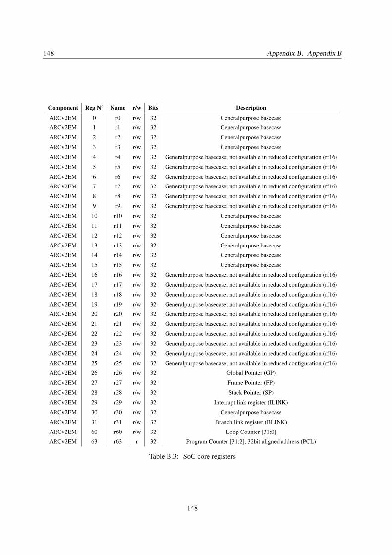
148 Appendix B. Appendix B
Component Reg N° Name r/w Bits Description
ARCv2EM 0 r0 r/w 32 Generalpurpose basecase
ARCv2EM 1 r1 r/w 32 Generalpurpose basecase
ARCv2EM 2 r2 r/w 32 Generalpurpose basecase
ARCv2EM 3 r3 r/w 32 Generalpurpose basecase
ARCv2EM 4 r4 r/w 32 Generalpurpose basecase; not available in reduced configuration (rf16)
ARCv2EM 5 r5 r/w 32 Generalpurpose basecase; not available in reduced configuration (rf16)
ARCv2EM 6 r6 r/w 32 Generalpurpose basecase; not available in reduced configuration (rf16)
ARCv2EM 7 r7 r/w 32 Generalpurpose basecase; not available in reduced configuration (rf16)
ARCv2EM 8 r8 r/w 32 Generalpurpose basecase; not available in reduced configuration (rf16)
ARCv2EM 9 r9 r/w 32 Generalpurpose basecase; not available in reduced configuration (rf16)
ARCv2EM 10 r10 r/w 32 Generalpurpose basecase
ARCv2EM 11 r11 r/w 32 Generalpurpose basecase
ARCv2EM 12 r12 r/w 32 Generalpurpose basecase
ARCv2EM 13 r13 r/w 32 Generalpurpose basecase
ARCv2EM 14 r14 r/w 32 Generalpurpose basecase
ARCv2EM 15 r15 r/w 32 Generalpurpose basecase
ARCv2EM 16 r16 r/w 32 Generalpurpose basecase; not available in reduced configuration (rf16)
ARCv2EM 17 r17 r/w 32 Generalpurpose basecase; not available in reduced configuration (rf16)
ARCv2EM 18 r18 r/w 32 Generalpurpose basecase; not available in reduced configuration (rf16)
ARCv2EM 19 r19 r/w 32 Generalpurpose basecase; not available in reduced configuration (rf16)
ARCv2EM 20 r20 r/w 32 Generalpurpose basecase; not available in reduced configuration (rf16)
ARCv2EM 21 r21 r/w 32 Generalpurpose basecase; not available in reduced configuration (rf16)
ARCv2EM 22 r22 r/w 32 Generalpurpose basecase; not available in reduced configuration (rf16)
ARCv2EM 23 r23 r/w 32 Generalpurpose basecase; not available in reduced configuration (rf16)
ARCv2EM 24 r24 r/w 32 Generalpurpose basecase; not available in reduced configuration (rf16)
ARCv2EM 25 r25 r/w 32 Generalpurpose basecase; not available in reduced configuration (rf16)
ARCv2EM 26 r26 r/w 32 Global Pointer (GP)
ARCv2EM 27 r27 r/w 32 Frame Pointer (FP)
ARCv2EM 28 r28 r/w 32 Stack Pointer (SP)
ARCv2EM 29 r29 r/w 32 Interrupt link register (ILINK)
ARCv2EM 30 r30 r/w 32 Generalpurpose basecase
ARCv2EM 31 r31 r/w 32 Branch link register (BLINK)
ARCv2EM 60 r60 r/w 32 Loop Counter [31:0]
ARCv2EM 63 r63 r 32 Program Counter [31:2], 32bit aligned address (PCL)
Table B.3: SoC core registers
148
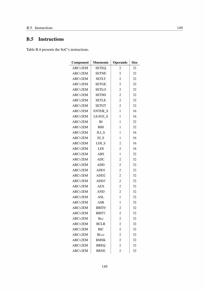
B.5. Instructions 149
B.5 Instructions
Table B.4 presents the SoC’s instructions.
Component Mnemonic Operands SizeARCv2EM SETEQ 2 32
ARCv2EM SETNE 2 32
ARCv2EM SETLT 2 32
ARCv2EM SETGE 2 32
ARCv2EM SETLO 2 32
ARCv2EM SETHS 2 32
ARCv2EM SETLE 2 32
ARCv2EM SETGT 2 32
ARCv2EM ENTER_S 1 16
ARCv2EM LEAVE_S 1 16
ARCv2EM BI 1 32
ARCv2EM BIH 1 32
ARCv2EM JLI_S 1 16
ARCv2EM EI_S 1 16
ARCv2EM LDI_S 2 16
ARCv2EM LDI 2 16
ARCv2EM ABS 1 32
ARCv2EM ADC 2 32
ARCv2EM ADD 2 32
ARCv2EM ADD1 2 32
ARCv2EM ADD2 2 32
ARCv2EM ADD3 2 32
ARCv2EM AEX 2 32
ARCv2EM AND 2 32
ARCv2EM ASL 1 32
ARCv2EM ASR 1 32
ARCv2EM BBIT0 2 32
ARCv2EM BBIT1 2 32
ARCv2EM Bcc 2 32
ARCv2EM BCLR 2 32
ARCv2EM BIC 2 32
ARCv2EM BLcc 2 32
ARCv2EM BMSK 2 32
ARCv2EM BREQ 2 32
ARCv2EM BRNE 2 32
149
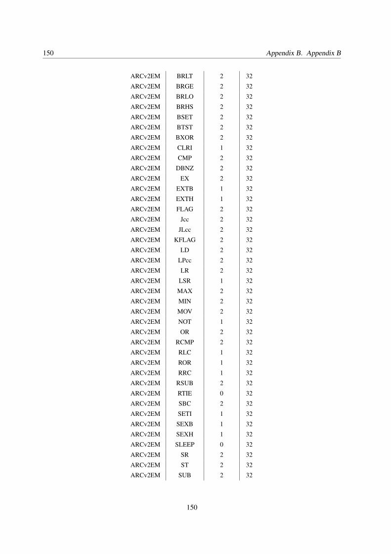
150 Appendix B. Appendix B
ARCv2EM BRLT 2 32
ARCv2EM BRGE 2 32
ARCv2EM BRLO 2 32
ARCv2EM BRHS 2 32
ARCv2EM BSET 2 32
ARCv2EM BTST 2 32
ARCv2EM BXOR 2 32
ARCv2EM CLRI 1 32
ARCv2EM CMP 2 32
ARCv2EM DBNZ 2 32
ARCv2EM EX 2 32
ARCv2EM EXTB 1 32
ARCv2EM EXTH 1 32
ARCv2EM FLAG 2 32
ARCv2EM Jcc 2 32
ARCv2EM JLcc 2 32
ARCv2EM KFLAG 2 32
ARCv2EM LD 2 32
ARCv2EM LPcc 2 32
ARCv2EM LR 2 32
ARCv2EM LSR 1 32
ARCv2EM MAX 2 32
ARCv2EM MIN 2 32
ARCv2EM MOV 2 32
ARCv2EM NOT 1 32
ARCv2EM OR 2 32
ARCv2EM RCMP 2 32
ARCv2EM RLC 1 32
ARCv2EM ROR 1 32
ARCv2EM RRC 1 32
ARCv2EM RSUB 2 32
ARCv2EM RTIE 0 32
ARCv2EM SBC 2 32
ARCv2EM SETI 1 32
ARCv2EM SEXB 1 32
ARCv2EM SEXH 1 32
ARCv2EM SLEEP 0 32
ARCv2EM SR 2 32
ARCv2EM ST 2 32
ARCv2EM SUB 2 32
150
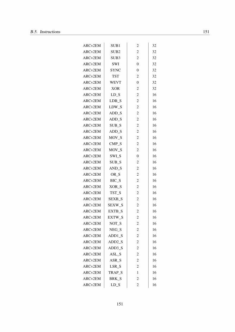
B.5. Instructions 151
ARCv2EM SUB1 2 32
ARCv2EM SUB2 2 32
ARCv2EM SUB3 2 32
ARCv2EM SWI 0 32
ARCv2EM SYNC 0 32
ARCv2EM TST 2 32
ARCv2EM WEVT 0 32
ARCv2EM XOR 2 32
ARCv2EM LD_S 2 16
ARCv2EM LDB_S 2 16
ARCv2EM LDW_S 2 16
ARCv2EM ADD_S 2 16
ARCv2EM ADD_S 2 16
ARCv2EM SUB_S 2 16
ARCv2EM ADD_S 2 16
ARCv2EM MOV_S 2 16
ARCv2EM CMP_S 2 16
ARCv2EM MOV_S 2 16
ARCv2EM SWI_S 0 16
ARCv2EM SUB_S 2 16
ARCv2EM AND_S 2 16
ARCv2EM OR_S 2 16
ARCv2EM BIC_S 2 16
ARCv2EM XOR_S 2 16
ARCv2EM TST_S 2 16
ARCv2EM SEXB_S 2 16
ARCv2EM SEXW_S 2 16
ARCv2EM EXTB_S 2 16
ARCv2EM EXTW_S 2 16
ARCv2EM NOT_S 2 16
ARCv2EM NEG_S 2 16
ARCv2EM ADD1_S 2 16
ARCv2EM ADD2_S 2 16
ARCv2EM ADD3_S 2 16
ARCv2EM ASL_S 2 16
ARCv2EM ASR_S 2 16
ARCv2EM LSR_S 2 16
ARCv2EM TRAP_S 1 16
ARCv2EM BRK_S 2 16
ARCv2EM LD_S 2 16
151
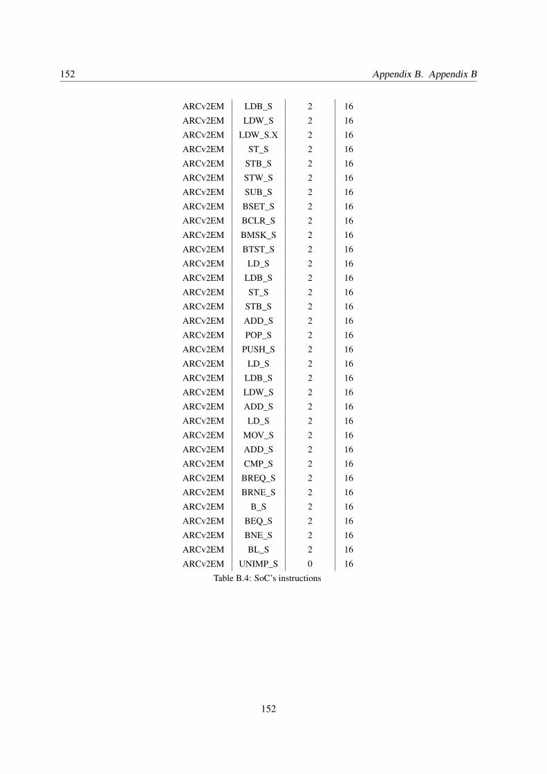
152 Appendix B. Appendix B
ARCv2EM LDB_S 2 16
ARCv2EM LDW_S 2 16
ARCv2EM LDW_S.X 2 16
ARCv2EM ST_S 2 16
ARCv2EM STB_S 2 16
ARCv2EM STW_S 2 16
ARCv2EM SUB_S 2 16
ARCv2EM BSET_S 2 16
ARCv2EM BCLR_S 2 16
ARCv2EM BMSK_S 2 16
ARCv2EM BTST_S 2 16
ARCv2EM LD_S 2 16
ARCv2EM LDB_S 2 16
ARCv2EM ST_S 2 16
ARCv2EM STB_S 2 16
ARCv2EM ADD_S 2 16
ARCv2EM POP_S 2 16
ARCv2EM PUSH_S 2 16
ARCv2EM LD_S 2 16
ARCv2EM LDB_S 2 16
ARCv2EM LDW_S 2 16
ARCv2EM ADD_S 2 16
ARCv2EM LD_S 2 16
ARCv2EM MOV_S 2 16
ARCv2EM ADD_S 2 16
ARCv2EM CMP_S 2 16
ARCv2EM BREQ_S 2 16
ARCv2EM BRNE_S 2 16
ARCv2EM B_S 2 16
ARCv2EM BEQ_S 2 16
ARCv2EM BNE_S 2 16
ARCv2EM BL_S 2 16
ARCv2EM UNIMP_S 0 16
Table B.4: SoC’s instructions
152
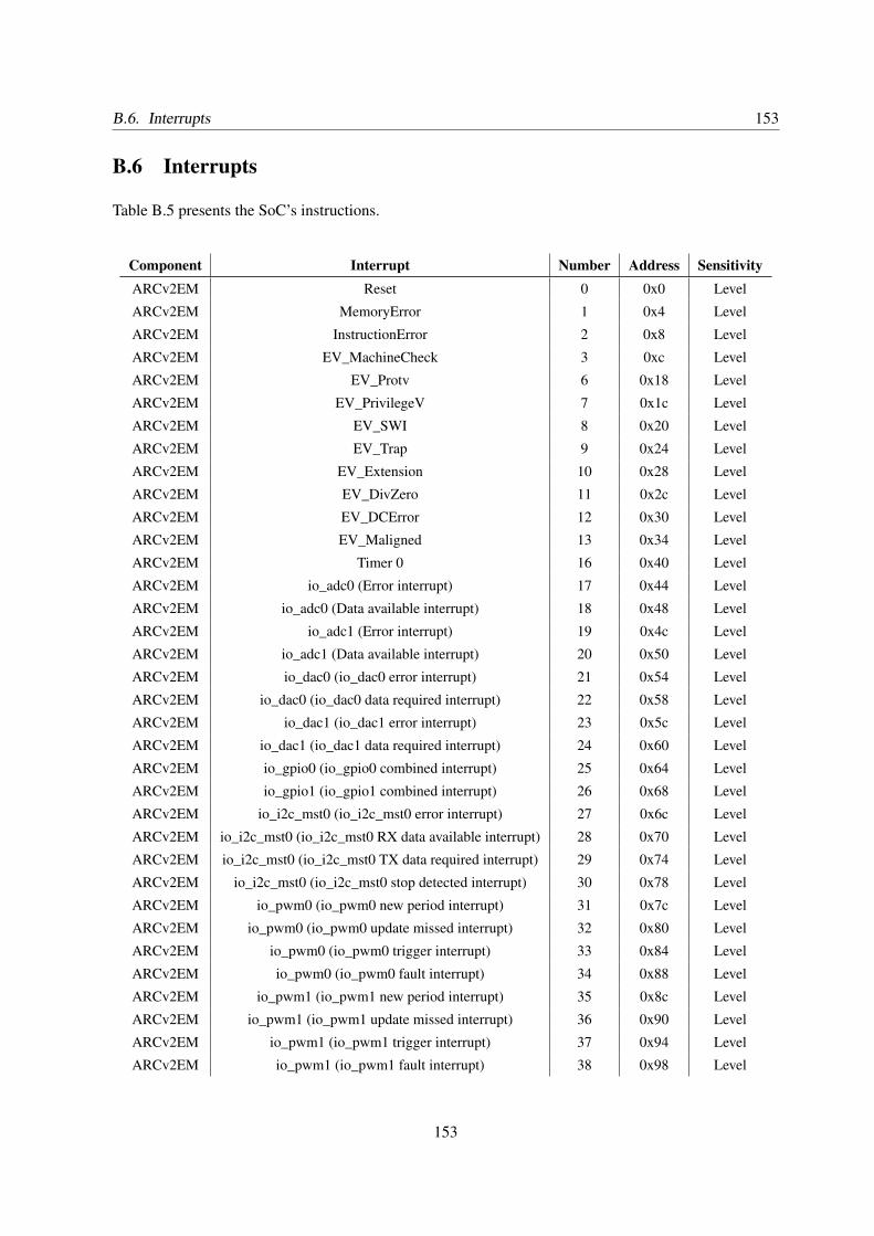
B.6. Interrupts 153
B.6 Interrupts
Table B.5 presents the SoC’s instructions.
Component Interrupt Number Address SensitivityARCv2EM Reset 0 0x0 Level
ARCv2EM MemoryError 1 0x4 Level
ARCv2EM InstructionError 2 0x8 Level
ARCv2EM EV_MachineCheck 3 0xc Level
ARCv2EM EV_Protv 6 0x18 Level
ARCv2EM EV_PrivilegeV 7 0x1c Level
ARCv2EM EV_SWI 8 0x20 Level
ARCv2EM EV_Trap 9 0x24 Level
ARCv2EM EV_Extension 10 0x28 Level
ARCv2EM EV_DivZero 11 0x2c Level
ARCv2EM EV_DCError 12 0x30 Level
ARCv2EM EV_Maligned 13 0x34 Level
ARCv2EM Timer 0 16 0x40 Level
ARCv2EM io_adc0 (Error interrupt) 17 0x44 Level
ARCv2EM io_adc0 (Data available interrupt) 18 0x48 Level
ARCv2EM io_adc1 (Error interrupt) 19 0x4c Level
ARCv2EM io_adc1 (Data available interrupt) 20 0x50 Level
ARCv2EM io_dac0 (io_dac0 error interrupt) 21 0x54 Level
ARCv2EM io_dac0 (io_dac0 data required interrupt) 22 0x58 Level
ARCv2EM io_dac1 (io_dac1 error interrupt) 23 0x5c Level
ARCv2EM io_dac1 (io_dac1 data required interrupt) 24 0x60 Level
ARCv2EM io_gpio0 (io_gpio0 combined interrupt) 25 0x64 Level
ARCv2EM io_gpio1 (io_gpio1 combined interrupt) 26 0x68 Level
ARCv2EM io_i2c_mst0 (io_i2c_mst0 error interrupt) 27 0x6c Level
ARCv2EM io_i2c_mst0 (io_i2c_mst0 RX data available interrupt) 28 0x70 Level
ARCv2EM io_i2c_mst0 (io_i2c_mst0 TX data required interrupt) 29 0x74 Level
ARCv2EM io_i2c_mst0 (io_i2c_mst0 stop detected interrupt) 30 0x78 Level
ARCv2EM io_pwm0 (io_pwm0 new period interrupt) 31 0x7c Level
ARCv2EM io_pwm0 (io_pwm0 update missed interrupt) 32 0x80 Level
ARCv2EM io_pwm0 (io_pwm0 trigger interrupt) 33 0x84 Level
ARCv2EM io_pwm0 (io_pwm0 fault interrupt) 34 0x88 Level
ARCv2EM io_pwm1 (io_pwm1 new period interrupt) 35 0x8c Level
ARCv2EM io_pwm1 (io_pwm1 update missed interrupt) 36 0x90 Level
ARCv2EM io_pwm1 (io_pwm1 trigger interrupt) 37 0x94 Level
ARCv2EM io_pwm1 (io_pwm1 fault interrupt) 38 0x98 Level
153
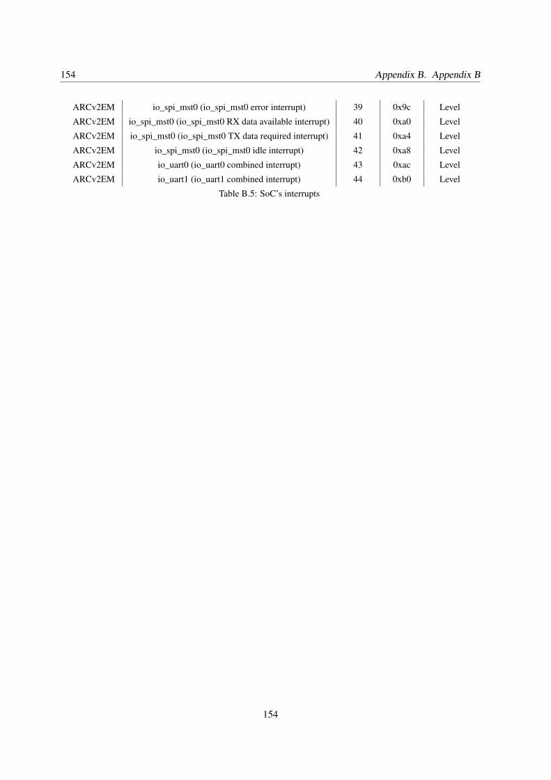
154 Appendix B. Appendix B
ARCv2EM io_spi_mst0 (io_spi_mst0 error interrupt) 39 0x9c Level
ARCv2EM io_spi_mst0 (io_spi_mst0 RX data available interrupt) 40 0xa0 Level
ARCv2EM io_spi_mst0 (io_spi_mst0 TX data required interrupt) 41 0xa4 Level
ARCv2EM io_spi_mst0 (io_spi_mst0 idle interrupt) 42 0xa8 Level
ARCv2EM io_uart0 (io_uart0 combined interrupt) 43 0xac Level
ARCv2EM io_uart1 (io_uart1 combined interrupt) 44 0xb0 Level
Table B.5: SoC’s interrupts
154
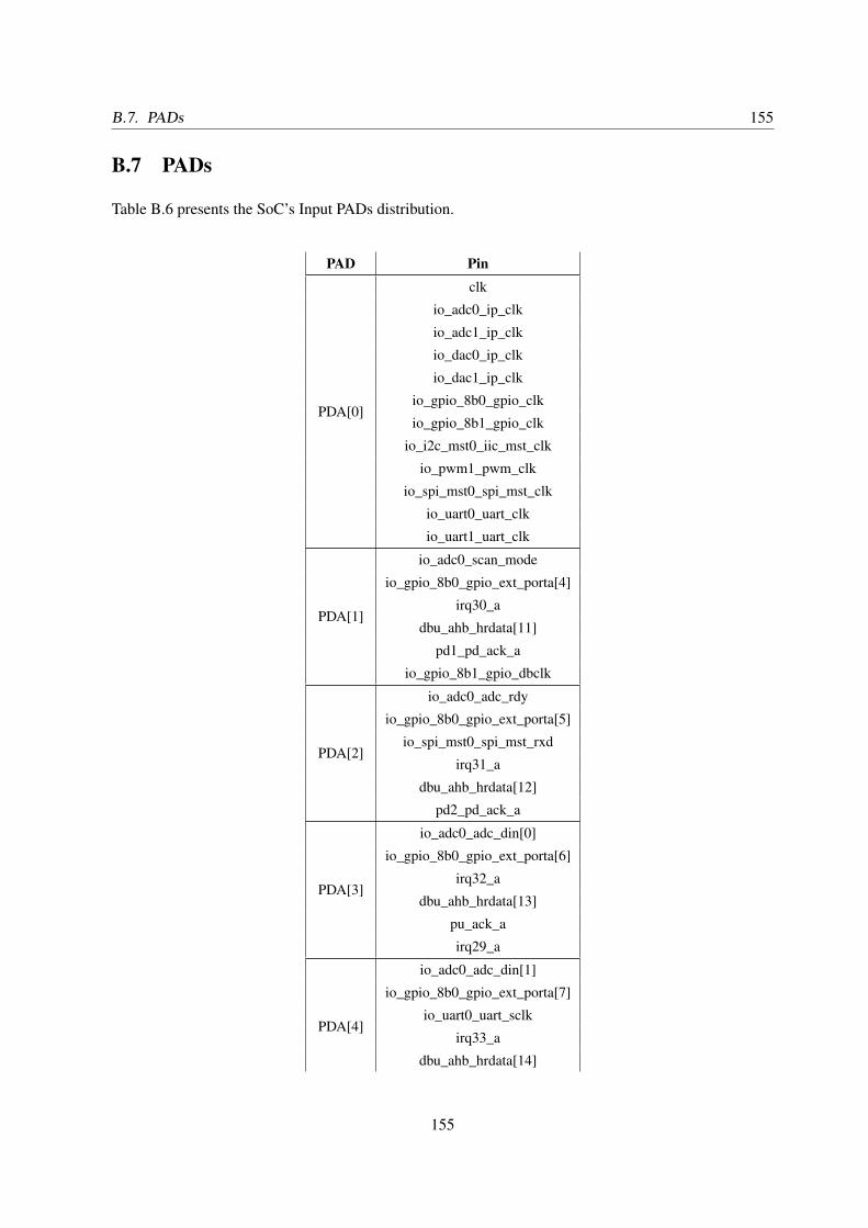
B.7. PADs 155
B.7 PADs
Table B.6 presents the SoC’s Input PADs distribution.
PAD Pin
PDA[0]
clk
io_adc0_ip_clk
io_adc1_ip_clk
io_dac0_ip_clk
io_dac1_ip_clk
io_gpio_8b0_gpio_clk
io_gpio_8b1_gpio_clk
io_i2c_mst0_iic_mst_clk
io_pwm1_pwm_clk
io_spi_mst0_spi_mst_clk
io_uart0_uart_clk
io_uart1_uart_clk
PDA[1]
io_adc0_scan_mode
io_gpio_8b0_gpio_ext_porta[4]
irq30_a
dbu_ahb_hrdata[11]
pd1_pd_ack_a
io_gpio_8b1_gpio_dbclk
PDA[2]
io_adc0_adc_rdy
io_gpio_8b0_gpio_ext_porta[5]
io_spi_mst0_spi_mst_rxd
irq31_a
dbu_ahb_hrdata[12]
pd2_pd_ack_a
PDA[3]
io_adc0_adc_din[0]
io_gpio_8b0_gpio_ext_porta[6]
irq32_a
dbu_ahb_hrdata[13]
pu_ack_a
irq29_a
PDA[4]
io_adc0_adc_din[1]
io_gpio_8b0_gpio_ext_porta[7]
io_uart0_uart_sclk
irq33_a
dbu_ahb_hrdata[14]
155
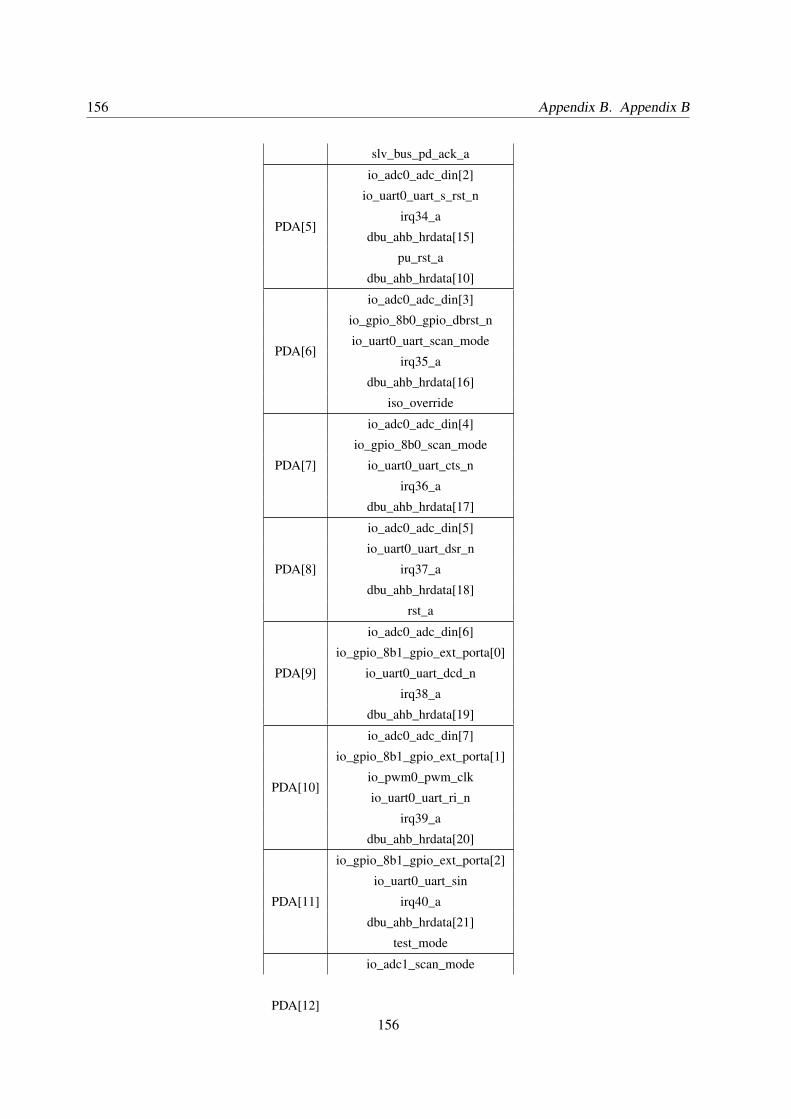
156 Appendix B. Appendix B
slv_bus_pd_ack_a
PDA[5]
io_adc0_adc_din[2]
io_uart0_uart_s_rst_n
irq34_a
dbu_ahb_hrdata[15]
pu_rst_a
dbu_ahb_hrdata[10]
PDA[6]
io_adc0_adc_din[3]
io_gpio_8b0_gpio_dbrst_n
io_uart0_uart_scan_mode
irq35_a
dbu_ahb_hrdata[16]
iso_override
PDA[7]
io_adc0_adc_din[4]
io_gpio_8b0_scan_mode
io_uart0_uart_cts_n
irq36_a
dbu_ahb_hrdata[17]
PDA[8]
io_adc0_adc_din[5]
io_uart0_uart_dsr_n
irq37_a
dbu_ahb_hrdata[18]
rst_a
PDA[9]
io_adc0_adc_din[6]
io_gpio_8b1_gpio_ext_porta[0]
io_uart0_uart_dcd_n
irq38_a
dbu_ahb_hrdata[19]
PDA[10]
io_adc0_adc_din[7]
io_gpio_8b1_gpio_ext_porta[1]
io_pwm0_pwm_clk
io_uart0_uart_ri_n
irq39_a
dbu_ahb_hrdata[20]
PDA[11]
io_gpio_8b1_gpio_ext_porta[2]
io_uart0_uart_sin
irq40_a
dbu_ahb_hrdata[21]
test_mode
PDA[12]
io_adc1_scan_mode
156
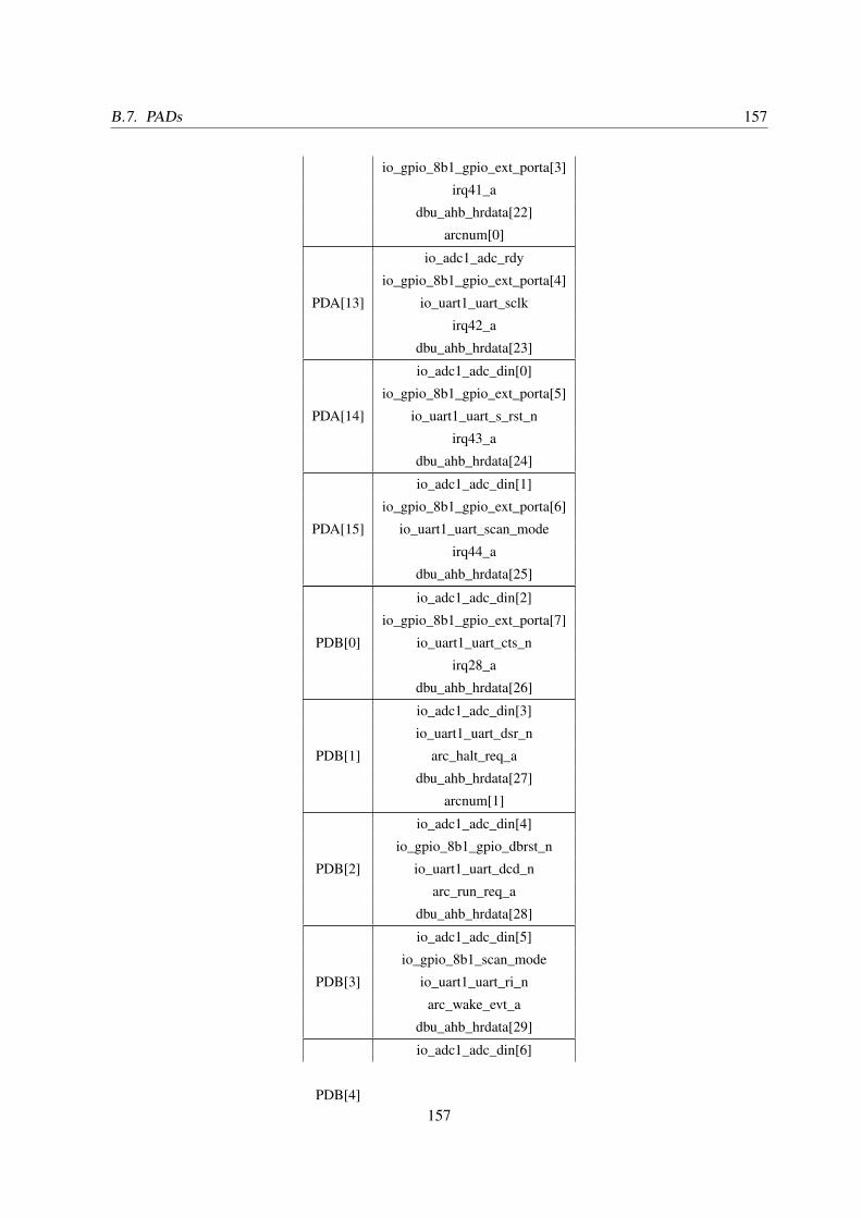
B.7. PADs 157
io_gpio_8b1_gpio_ext_porta[3]
irq41_a
dbu_ahb_hrdata[22]
arcnum[0]
PDA[13]
io_adc1_adc_rdy
io_gpio_8b1_gpio_ext_porta[4]
io_uart1_uart_sclk
irq42_a
dbu_ahb_hrdata[23]
PDA[14]
io_adc1_adc_din[0]
io_gpio_8b1_gpio_ext_porta[5]
io_uart1_uart_s_rst_n
irq43_a
dbu_ahb_hrdata[24]
PDA[15]
io_adc1_adc_din[1]
io_gpio_8b1_gpio_ext_porta[6]
io_uart1_uart_scan_mode
irq44_a
dbu_ahb_hrdata[25]
PDB[0]
io_adc1_adc_din[2]
io_gpio_8b1_gpio_ext_porta[7]
io_uart1_uart_cts_n
irq28_a
dbu_ahb_hrdata[26]
PDB[1]
io_adc1_adc_din[3]
io_uart1_uart_dsr_n
arc_halt_req_a
dbu_ahb_hrdata[27]
arcnum[1]
PDB[2]
io_adc1_adc_din[4]
io_gpio_8b1_gpio_dbrst_n
io_uart1_uart_dcd_n
arc_run_req_a
dbu_ahb_hrdata[28]
PDB[3]
io_adc1_adc_din[5]
io_gpio_8b1_scan_mode
io_uart1_uart_ri_n
arc_wake_evt_a
dbu_ahb_hrdata[29]
PDB[4]
io_adc1_adc_din[6]
157
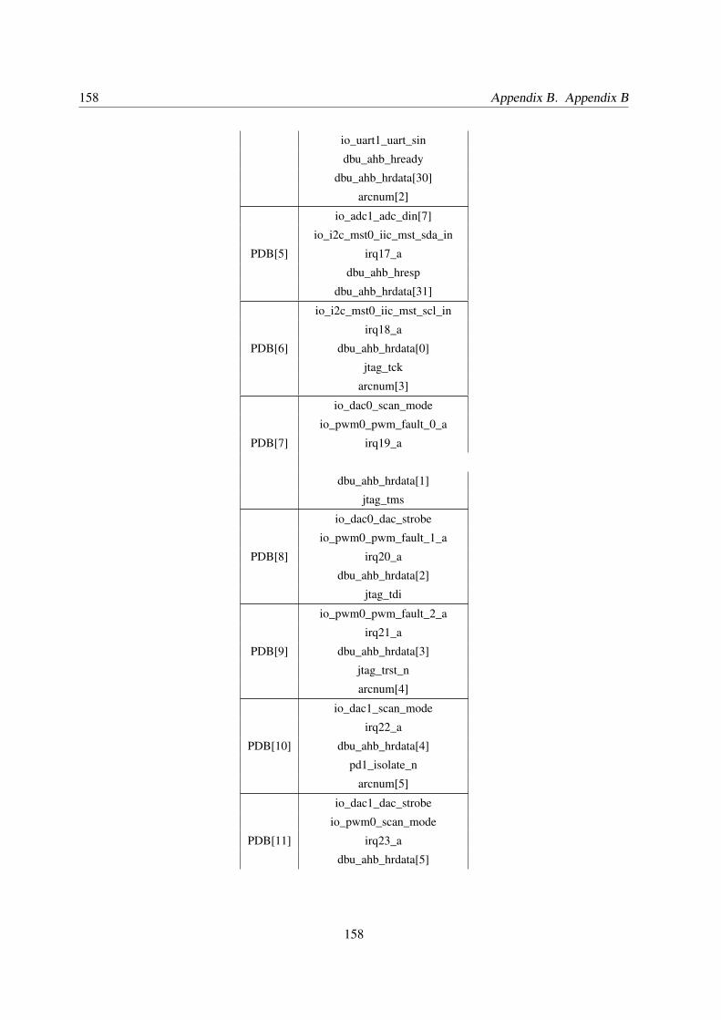
158 Appendix B. Appendix B
io_uart1_uart_sin
dbu_ahb_hready
dbu_ahb_hrdata[30]
arcnum[2]
PDB[5]
io_adc1_adc_din[7]
io_i2c_mst0_iic_mst_sda_in
irq17_a
dbu_ahb_hresp
dbu_ahb_hrdata[31]
PDB[6]
io_i2c_mst0_iic_mst_scl_in
irq18_a
dbu_ahb_hrdata[0]
jtag_tck
arcnum[3]
PDB[7]
io_dac0_scan_mode
io_pwm0_pwm_fault_0_a
irq19_a
dbu_ahb_hrdata[1]
jtag_tms
PDB[8]
io_dac0_dac_strobe
io_pwm0_pwm_fault_1_a
irq20_a
dbu_ahb_hrdata[2]
jtag_tdi
PDB[9]
io_pwm0_pwm_fault_2_a
irq21_a
dbu_ahb_hrdata[3]
jtag_trst_n
arcnum[4]
PDB[10]
io_dac1_scan_mode
irq22_a
dbu_ahb_hrdata[4]
pd1_isolate_n
arcnum[5]
PDB[11]
io_dac1_dac_strobe
io_pwm0_scan_mode
irq23_a
dbu_ahb_hrdata[5]
158
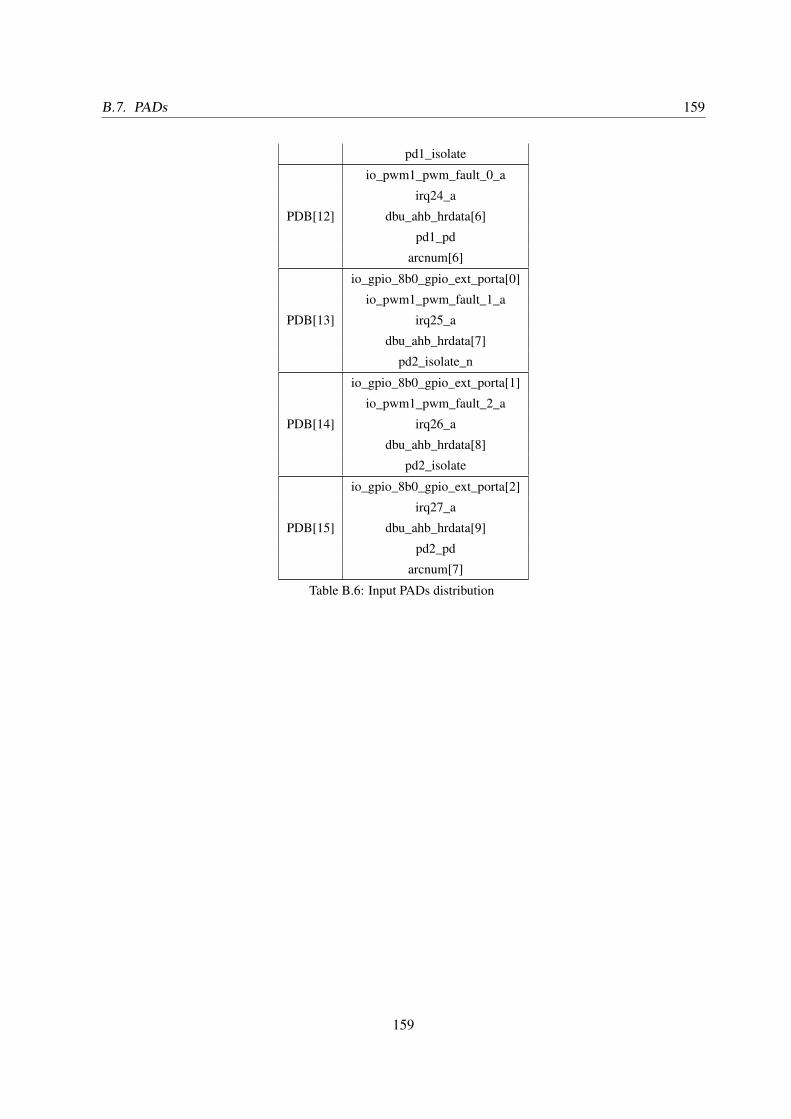
B.7. PADs 159
pd1_isolate
PDB[12]
io_pwm1_pwm_fault_0_a
irq24_a
dbu_ahb_hrdata[6]
pd1_pd
arcnum[6]
PDB[13]
io_gpio_8b0_gpio_ext_porta[0]
io_pwm1_pwm_fault_1_a
irq25_a
dbu_ahb_hrdata[7]
pd2_isolate_n
PDB[14]
io_gpio_8b0_gpio_ext_porta[1]
io_pwm1_pwm_fault_2_a
irq26_a
dbu_ahb_hrdata[8]
pd2_isolate
PDB[15]
io_gpio_8b0_gpio_ext_porta[2]
irq27_a
dbu_ahb_hrdata[9]
pd2_pd
arcnum[7]
Table B.6: Input PADs distribution
159

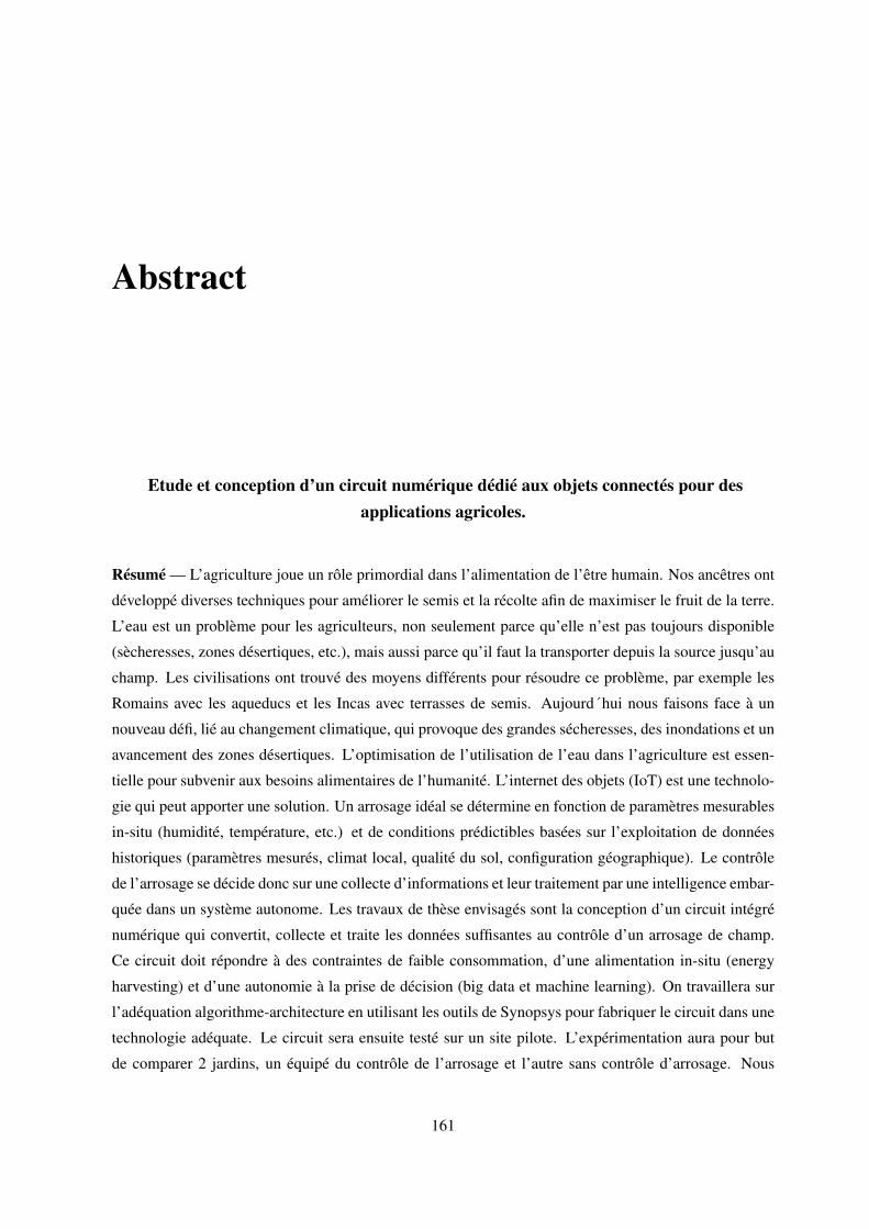
Abstract
Etude et conception d’un circuit numérique dédié aux objets connectés pour desapplications agricoles.
Résumé — L’agriculture joue un rôle primordial dans l’alimentation de l’être humain. Nos ancêtres ont
développé diverses techniques pour améliorer le semis et la récolte afin de maximiser le fruit de la terre.
L’eau est un problème pour les agriculteurs, non seulement parce qu’elle n’est pas toujours disponible
(sècheresses, zones désertiques, etc.), mais aussi parce qu’il faut la transporter depuis la source jusqu’au
champ. Les civilisations ont trouvé des moyens différents pour résoudre ce problème, par exemple les
Romains avec les aqueducs et les Incas avec terrasses de semis. Aujourd´hui nous faisons face à un
nouveau défi, lié au changement climatique, qui provoque des grandes sécheresses, des inondations et un
avancement des zones désertiques. L’optimisation de l’utilisation de l’eau dans l’agriculture est essen-
tielle pour subvenir aux besoins alimentaires de l’humanité. L’internet des objets (IoT) est une technolo-
gie qui peut apporter une solution. Un arrosage idéal se détermine en fonction de paramètres mesurables
in-situ (humidité, température, etc.) et de conditions prédictibles basées sur l’exploitation de données
historiques (paramètres mesurés, climat local, qualité du sol, configuration géographique). Le contrôle
de l’arrosage se décide donc sur une collecte d’informations et leur traitement par une intelligence embar-
quée dans un système autonome. Les travaux de thèse envisagés sont la conception d’un circuit intégré
numérique qui convertit, collecte et traite les données suffisantes au contrôle d’un arrosage de champ.
Ce circuit doit répondre à des contraintes de faible consommation, d’une alimentation in-situ (energy
harvesting) et d’une autonomie à la prise de décision (big data et machine learning). On travaillera sur
l’adéquation algorithme-architecture en utilisant les outils de Synopsys pour fabriquer le circuit dans une
technologie adéquate. Le circuit sera ensuite testé sur un site pilote. L’expérimentation aura pour but
de comparer 2 jardins, un équipé du contrôle de l’arrosage et l’autre sans contrôle d’arrosage. Nous
161
162 Appendix B. Appendix B
mesurerons l’apprentissage du système sur une longue durée afin de quantifier la réduction de la con-
sommation d’eau à rendement égale.
Mots clés — Internet des choses, Agriculture de Precision, capteurs, croissance des plantes.
Design of an integrated digital circuit for the Internet of Things (IoT) applied toagronomy.
Abstract — Agriculture plays a key role in humans’ nutrition. Our ancestors have developed various
techniques to improve seedling and harvesting to maximize the fruit of their land. Water is a problem
for farmers, not only because it is not always available (droughts, desert areas, etc.), but also because
it has to be transported from the source to the field. Civilizations have found different ways to solve
this problem, for example the Romans with the aqueducts and the Incas with terraced levels of seedlings.
Nowadays, we are facing a new challenge, linked to climate change, which causes severe droughts, floods
and the progression of desert areas. Optimizing the use of water in agriculture is essential to meet the
food requirements of humankind. The Internet of Things (IoT) is a technology that can provide a solu-
tion. An ideal irrigation is determined according to in-situ parameters (humidity, temperature, etc.) and
predictable conditions based on historical data (measured parameters, local climate, soil quality, geo-
graphical configuration). The control of irrigation is therefore decided on a collection of information and
their treatment by an intelligence embedded in an autonomous system. The thesis work envisaged is the
design of a digital integrated circuit that converts, collects and processes sufficient data to control a field
irrigation. This circuit must respond to low power consumption constraints, in-situ energy harvesting and
decision-making autonomy (big data and machine learning). We will work on the algorithm-architecture
adequacy using the Synopsys tools to fabricate the circuit in a suitable technology. The circuit will then
be tested on an experimental site. The experiment will aim to compare 2 gardens, one equipped with
control of watering and the other without control of watering. We will measure system learning over a
long period of time to quantify the reduction in water consumption with equal yield.
Keywords — Internet of Things, Precision agriculture, sensors, crop growth.
162

B.7. PADs 163
163
Related Documents