Luminescence Lifetime Imaging Microscopy by Confocal ...

Luminescence Lifetime Imaging Microscopy by Confocal Pinhole Shifting (LLIM-CPS)

by

Venkat K. Ramshesh A dissertation submitted to the faculty of the University of North Carolina at Chapel Hill in partial fulfillment of the requirements for the degree of Doctor of Philosophy in the Department of Biomedical Engineering.

Chapel Hill 2007

Approved by:

John J. Lemasters Stephen B. Knisley David S. Lalush M. Joseph Costello

Caterina M. Gallippi

©2007

Venkat K. Ramshesh

ALL RIGHTS RESERVED

ii

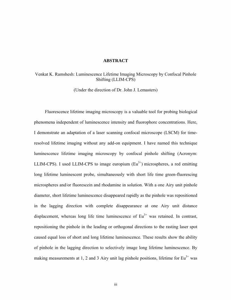
ABSTRACT

Venkat K. Ramshesh: Luminescence Lifetime Imaging Microscopy by Confocal Pinhole

Shifting (LLIM-CPS)

(Under the direction of Dr. John J. Lemasters)

Fluorescence lifetime imaging microscopy is a valuable tool for probing biological

phenomena independent of luminescence intensity and fluorophore concentrations. Here,

I demonstrate an adaptation of a laser scanning confocal microscope (LSCM) for time-

resolved lifetime imaging without any add-on equipment. I have named this technique

luminescence lifetime imaging microscopy by confocal pinhole shifting (Acronym:

LLIM-CPS). I used LLIM-CPS to image europium (Eu3+) microspheres, a red emitting

long lifetime luminescent probe, simultaneously with short life time green-fluorescing

microspheres and/or fluorescein and rhodamine in solution. With a one Airy unit pinhole

diameter, short lifetime luminescence disappeared rapidly as the pinhole was repositioned

in the lagging direction with complete disappearance at one Airy unit distance

displacement, whereas long life time luminescence of Eu3+ was retained. In contrast,

repositioning the pinhole in the leading or orthogonal directions to the rasting laser spot

caused equal loss of short and long lifetime luminescence. These results show the ability

of pinhole in the lagging direction to selectively image long lifetime luminescence. By

making measurements at 1, 2 and 3 Airy unit lag pinhole positions, lifetime for Eu3+ was

iii

estimated to be 270 µs. The effect of pinhole diameter and laser dwell times on LLIM-

CPS were studied. Pinhole diameters of 3 and 5 Airy units caused streaking of long

lifetime europium microspheres with a one Airy unit pinhole diameter resolving the

europium to its true diameter. Dwell times of 51 and 102 µs were required to image the

europium microspheres compared to the shorter 3 µs dwell time that could not image the

europium microspheres.

LLIM-CPS was used to quantify oxygen-dependent changes in intensity and

lifetime of Tris-4, 7 diphenyl 1, 10-phenanthroline ruthenium an oxygen sensing long

lifetime luminophore. LLIM-CPS images of heart cells in the presence of the oxygen-

sensing phosphorescent luminophore, PtTBP-AG2-PEG, visualized oxygen surrounding

the respiring cells. Thus, in this dissertation I have demonstrated an adaptation of a

LSCM to perform quantitative long lifetime luminescence imaging and presented a

biological application of oxygen sensing with this technique.

iv

ACKNOWLEDGEMENTS

I would like to dedicate this dissertation to my sister, brother-in-law and parents who

provided constant motivation, love and support. I would like to thank my advisor Dr.

John J. Lemasters for providing me with the opportunity to work in his laboratory and his

guidance and support. I would also like to express my gratitude to all my committee

members and the departments of Biomedical Engineering and Cell and Developmental

Biology at UNC-CH and department of Pharmaceutical Sciences at MUSC. I would like

to also thank all my laboratory members of the past several years. I also express my

gratitude to all my friends who have guided me in many ways.

vii

TABLE OF CONTENTS List of Figures …………………………………………………………………………...x List of Abbreviations and Symbols …………………………………………………...xii

Chapter

1. Introduction................................................................................................................... 1

1.1 Lifetime Imaging .......................................................................................................... 2 2. Background, Literature Review and Project Aims ................................................... 4

2.1 Light Microscopy.......................................................................................................... 4 2.2 Confocal Fluorescence Microscopy.............................................................................. 5

2.2.1 Laser Scanning Confocal Microscope ......................................................5

2.2.2 Spinning Disk Confocal Microscope ........................................................6

2.2.3 Applications of Confocal Microscopy ......................................................7

2.3 Pinhole Sizes in Specimen and Image Planes............................................................... 8 2.4 Multiphoton Excitation in Fluorescence Microscopy................................................. 10 2.4 Advances in Microscopy............................................................................................. 12 2.5 Fluorescence Lifetime Imaging Microscopy .............................................................. 13

2.5.1 Time-based Fluorescence Lifetime Imaging Microscopy ......................14

2.5.2 Frequency-based Fluorescence Lifetime Imaging Microscopy..............15

2.6 Fluorescence vs. Phosphorescence Lifetimes ............................................................. 15

viii

2.7 Oxygen Sensing Techniques....................................................................................... 17

2.7.1 Microsphectrophotometry.......................................................................17

2.7.2 Redox Fluorometry .................................................................................18

2.7.3 Oxygen Electrodes ..................................................................................18

2.7.4 Functional Magnetic Resonance Imaging...............................................19

2.7.5 Luminescence Based Oxygen Sensing ...................................................19

2.8 Mitochondrial Metabolism.......................................................................................... 21 2.9 Aims of Project ........................................................................................................... 23 2.10 Novelty of Project ..................................................................................................... 25 3. Methods and Materials............................................................................................... 38

3.1 Imaging of Long Lifetime Europium Microspheres and Short Lifetime Luminophores .................................................................................... 38 3.2 Imaging of Europium and Blue Microspheres............................................................ 39 3.3 Europium Slide preparation ........................................................................................ 39 3.4 Imaging of Oxygen Sensing Luminophores ............................................................... 40 3.5 Imaging PtTBP-AG2-PEG .......................................................................................... 40 3.6 Myocyte Isolation ....................................................................................................... 40 3.7 Tetramethylrhodamine Methylester Labeling............................................................. 41 3.8 Myocyte Imaging with Tetramethylrhodamine Methylester and PtTBP-AG2-PEG.................................................................................... 41 3.9 Agarose for Covering Myocytes................................................................................. 42 3.10 Software .................................................................................................................... 42 3.11 Luminophores and Chemicals................................................................................... 42 4. Results .......................................................................................................................... 44

4.1 Phosphorescence Lifetime Imaging Microscopy by Confocal Pinhole Shifting................................................................................................. 44

vii

4.2 Two-photon Excitation of Europium.......................................................................... 45 4.3 Images of Long Lifetime Europium and Short Lifetime Probes after Pinhole Shifting.................................................................... 46 4.4 Selection of Laser Dwell Time for Long Lifetime Imaging....................................... 49 4.5 Measurement of Lifetime using Phosphorescence Lifetime Imaging Microscopy by Pinhole Shifting ......................................................................... 51 4.6 Intensity of Europium and Green Microspheres for Different Pinhole Positions ......................................................................................... 53 4.7 Effect of Orthogonal Pinhole Shifts on Short and Long Lifetime Luminescence Measurements ................................................................................................................... 55 4.8 Effect of Pinhole Diameter on Long Lifetime Imaging.............................................. 56 4.9 Effect of Pinhole Diameter on Pinhole Shifting ......................................................... 58 4.10 Testing Oxyrase for Oxygen Removal ..................................................................... 61 4.11 Imaging Long Lifetime Oxygen Luminophores Using Luminescence Lifetime Imaging Microscopy by Confocal Pinhole Shifting ......................................................... 62

4.11.1 Tris-4, 7 diphenyl 1, 10-phenanthroline ruthenium (II)........................62

4.12 Oxygen Sensing Luminophore PtTBP-AG2-PEG .................................................... 65

4.12.1 PtTBP-AG2-PEG Response to Oxygen Change ...................................66

4.12.2 Oxygen Measurement in Myocytes Using PtTBP-AG2-PEG...............66

4.13 Discrepancy in Lifetime Measurements of Oxygen Sensors...................69

5. Discussion..................................................................................................................... 91

5.1 Principle of Long Lifetime Luminescence Imaging by Confocal Pinhole Shifting............................................................................................ 91 5.2 Multiphoton Excitation for Long Lifetime Imaging................................................... 92 5.3 Effect of Dwell Time on Lifetime Imaging ................................................................ 93 5.4 Measuring Lifetimes ................................................................................................... 94 5.5 Quantification of Pinhole Shifting .............................................................................. 95

viii

5.6 Effect of Pinhole Diameter on Lifetime Imaging ....................................................... 96 5.7 Imaging of the Long Lifetime Oxygen Luminophore tris-4, 7 diphenyl 1, 10-phenanthroline ruthenium ........................................................... 97 5.8 Oxygen Sensing Luminophore, PtTBP-AG2-PEG ..................................................... 99 5.9 Discrepancies in Lifetime Measurement .................................................................. 100 5.10 Lateral Shift in Images due to Pinhole Shifting...................................................... 101 5.11 Multiple Pinholes for LLIM-CPS ........................................................................... 101 5.12 Comparison with other Lifetime Techniques ......................................................... 102 5.13 Drawbacks of LLIM-CPS....................................................................................... 103 5.14 Conclusions............................................................................................................. 104 References...................................................................................................................... 106

ix

LIST OF FIGURES

2.1 Scheme of a laser scanning confocal fluorescence microscope.................................. 26

2.2 Scheme of a spinning disc confocal fluorescence microscope ................................... 27

2.3 Non-confocal and confocal with pinhole closed images of cultured myocytes.......... 28 2.4 Conventional and wide-field confocal reflected images of tilted microcuit............... 29 2.5 Jablosnki diagram illustrating the energy transitions in multiphoton excitation ........ 30 2.6 One and two-photon excited fluorescence emission from fluorescein ....................... 31 2.7 Decay response of a luminophore ...............................................................................32

2.8 Schematic of frequency based technique to measure lifetime .....................................33

2.9 Jablonski diagram ilustrating energy transitions in fluorescence and phosphorescence ....................................................................................34 2.10 Energy transitions in oxygen sensing with luminescent probes ................................35

2.11 Confocal images of myocytes labeled with Rhod 2-AM...........................................36

2.12 Average intenisty of Rhod 2-AM fluorescence in myocytes.................................... 37

4.1 Principle of luminescence lifetime imaging microscopy by confocal pinhole shifting ............................................................................................. 70 4.2 Plot of intensity of long lifetime europium microspheres with two-photon excitation........................................................................................................................... 71 4.3 Confocal images of europium and short lifetime luminophores................................. 72 4.4 Confocal images of europium and blue microspheres................................................ 73 4.5 Intensity of blue and europium micropheres at different dwell times .........................74

4.6 Illustration of pinhole shifting to measure lifetimes ...................................................75

4.7 Confocal images of europium micropsheres at different lag pinhole positions...........76

4.8 Lifetime plot of europium microspheres......................................................................77

x

4.9 Confocal images of europium and green microspheres for different parallel pinhole positions ...................................................................................................78 4.10 Plot of intensity of europium and green microspheres for different parallel pinhole positions ...................................................................................................79 4.11 Confocal images of europium and green microspheres for different orthogonal pinhole positions..............................................................................................80 4.12 Plot of intensity of europium and green micropsheres for different orthogonal pinhole psoitions..............................................................................................81 4.13 Confocal images of europium and blue micropsheres for different pinhole diameters .............................................................................................................. 82 4.14 Intensity of europium and green microspheres for different pinhole diameters .............................................................................................................. 83 4.15 Plot of oxygen consumption by oxyrase....................................................................84

4.16 Confocal images of TDPR using LLIM-CPS ...........................................................85

4.17 Lifetime plot of TDPR...............................................................................................86

4.18 Confocal images of PtTBP in air and oxygen-depleted medium...............................87

4.19 Confocal images of PtTBP and TMRM in myoyctes ................................................88

4.20 Confocal images of oxyphor G2 for different pinhole positions ...............................89

4.21 Lifetime plot of oxyphor G2 ……………………………………………………….90

xi

ABBREVIATIONS

FLIM Fluorescence lifetime imaging microscopy

LLIM-CPS Luminescence lifetime imaging microscopy by confocal pinhole shifting

DIC Differential interference contrast

3-D 3 dimension

LSCM Laser scanning confocal microscope

TMRM Tetramethylrhodamine methylester

NA Numerical aperture

NADH Nicotinamide adenine dinucleotide

NADPH Nicotinamide adenine dinucleotide phosphate-oxidase

FRAP Fluorescence recovery after photobleaching

FRET Fluorescence resonance energy transfer

TCSPC Time correlated single photon counting

FADH Flavin adenine dinucleotide

fMRI Functional magnetic resonance imaging

ATP Adenosine triphosphate

Eu3+ Europium

GmBH Gesellschaft mit beschränkter Haftung

Ti-Sapphire Titanium sapphire

TDPR tris-4, 7 diphenyl 1, 10-phenanthrolin ruthenium (II) complex

KRH Krebs-ringer-Hepes

xii

NaCl Sodium chloride

KCl Potassium chloride

CaCl2 Calcium chloride

Na2HPO4 Disodium phosphate

KH2PO4 Potassium phosphate

MgSO4 Magnesium sulphate

HEPES 4-(2-hydroxyethyl)-1-piperazineethanesulfonic acid

He-Ne Helium neon

xiii

CHAPTER 1

INTRODUCTION

In conventional fluorescence microscopy, the intensity and distribution of

fluorescence provide information about the biological structure and/or phenomena under

investigation. Extrinsically added fluorophores, engineered fluorescent proteins, and

tissue autofluorescence serve as sensors of biological phenomena. A sample is excited

with a suitable light source, and the resulting fluorescence is collected to characterize the

phenomena being investigated. The fluorescent images acquired are dependent on a

variety of factors, including the intensity of excitation light, fluorophore concentration,

detector gain, and photobleaching apart from the phenomena under investigation.

In quantititative fluorescence microscopy, fluorescence intensity can change

independently of the phenomenon being investigated. For example, leakage of

fluorophores, photobleaching and changes of cell shape can alter fluorescence

measurements independently of the biological parameter under study [1]. Ratio imaging

overcomes signal variations due to dye redistribution and photobleaching and is used

effectively to image calcium, pH and other cellular parameters [2] [3] [4]. However, the

spectral characteristics of many fluorophores are not amenable to ratio imaging.

An alternative approach is fluorescence lifetime imaging microscopy (FLIM) that

uses the lifetime of luminescence decay to visualize biological parameters of interest. In

this technique one uses the lifetime of a fluorophore to investigate a biological

phenomenon. Lifetime measurements are independent of the concentration of

luminophores (fluorophores and phosphors), excitation intensity, detector gain and other

factors that introduce artifacts in the intensity measurements [5]. For luminophores of

sufficiently different lifetimes, a single excitation source and detector can be used to

discriminate multiple luminophores of differing lifetimes but similar spectral

characteristics [6]. Lifetimes are however affected by substances and/or phenomena

known to alter decay times, acting as quenchers. These include the phenomena of

resonance energy transfer, collisional quenching, and temperature effects [7].

Applications of lifetime imaging include oxygen sensing, ion (Ca2+ and pH)

imaging, fluorescence resonance energy transfer with lifetime imaging, and tissue

endoscopy [8, 9]. Oxygen sensing fluorophores undergo quenching and decrease in

lifetime with increasing oxygen concentration [10]. Since the lifetime of the oxygen

sensitive luminophore is independent of the intensity of excitation light, detector gain,

and local fluorophore concentration, a change in its value reflects only changes in oxygen

concentration.

1.1 Lifetime Imaging

Fluorescence lifetime imaging microscopy (FLIM) combines fluorescence

microscopy with lifetime imaging in order to study phenomena such as oxygen sensing

2

and ion imaging [8]. However, FLIM instrumentation requires modifications and

expensive add-on equipment to the microscope and is not widely available [11]. For

instance, to adapt microscopes with ultrafast multiphoton lasers for FLIM in the

microsecond time scales typically found for oxygen sensing luminophores, modification

with cavity dumpers or pulse pickers is required to lower the repetition rate [12].

Here, I develop a time domain based FLIM technique for measuring lifetimes on

the microsecond time scale with sub-micron resolution by shifting the detection pinhole

of a confocal/multiphoton fluorescence microscope. I have done so without any

modifications or add-on equipment. I call this technique luminescence lifetime imaging

microscopy by confocal pinhole shifting (acronym: LLIM-CPS). My dissertation

demonstrates the development, implementation and characterization of LLIM-CPS and

its biological application to measure oxygen with oxygen sensing luminophores.

3

CHAPTER 2

BACKGROUND, LITERATURE REVIEW AND PROJECT AIMS

This chapter gives the background and literature review on the techniques used in

this dissertation project. The chapter also addresses the novelty and specific aims of my

project.

2.1 Light Microscopy

Light microscopy involves the interaction of light with biological specimens in

order to image micron-scaled phenomena. Traditional microscopy techniques like bright-

field, DIC, phase contrast and polarization microscopy use the absorption, transmission

and scattering of light by the specimen to provide the contrast required to image the

biological phenomena. These techniques have limitations for investigating physiological

phenomena in living cells and tissues, such as membrane potentials and ion transients.

The development of fluorescent microscopy together with the introduction of fluorescent

probes with sensitivity to specific physiological parameters now enables characterization

of a wide variety of cellular processes in living cells.

Initially, fluorescence microscopy was developed in the wide-field mode in which

fluorescence is collected from everywhere in the specimen after excitation with a suitable

light source. Wide-field fluorescence images suffer from the presence of out-of-focus

light that obscures observation of sub-micron structures like mitochondria, especially in

thicker specimens. This limitation of achievable resolution was a stimulus for the

development of techniques like confocal and multiphoton fluorescence microscopy.

2.2 Confocal Fluorescence Microscopy

A confocal fluorescence microscope is a modified wide-field fluorescence

microscope that excludes fluorescent and reflected light originating from out-of-focus

planes using a pinhole. By excluding light reaching the detector from out-of-focus planes

with the help of a pinhole, confocal microscopes achieve smaller depths of field, allowing

one to create thin optical sections through thick specimens [13, 14]. This enables one to

perform 3-D imaging of thick biological samples. The confocal principle was first

described by Minsky in 1955 [15]. Minsky's motivation to develop such a system was a

desire to obtain an image of a slice of a specimen without the distracting presence of out-

of-focus light. While a confocal microscope can be used in fluorescent and reflected

modes, my project focuses on its use in the fluorescence mode. The two commonly used

versions of a confocal fluorescence microscope are the laser scanning and the spinning

disc confocal microscope [16].

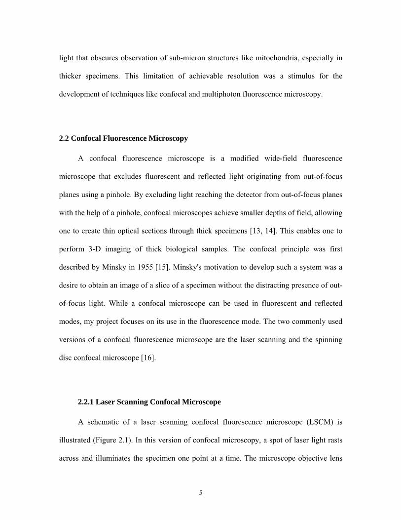
2.2.1 Laser Scanning Confocal Microscope

A schematic of a laser scanning confocal fluorescence microscope (LSCM) is

illustrated (Figure 2.1). In this version of confocal microscopy, a spot of laser light rasts

across and illuminates the specimen one point at a time. The microscope objective lens

5

acts to focus the laser light to a small spot in the specimen. Returning fluorescence is

collected by the same objective and descanned by the scan generator to be projected onto

a pinhole. One can observe from Figure 2.1 that only in-focus light manages to pass

through the pinhole unobstructed, whereas nearly all out-of-focus light misses the pinhole

and fails to reach the photodetector beyond. The consequence of the pinhole is an

improvement in axial resolution compared to a wide field fluorescence microscope and

nearly complete elimination of out-of-focus light. By rasting the laser spot across the

specimen using the scan generator an image of the entire specimen is created.

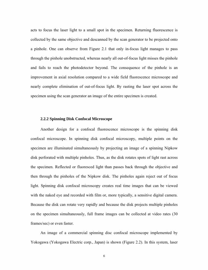
2.2.2 Spinning Disk Confocal Microscope

Another design for a confocal fluorescence microscope is the spinning disk

confocal microscope. In spinning disk confocal microscopy, multiple points on the

specimen are illuminated simultaneously by projecting an image of a spinning Nipkow

disk perforated with multiple pinholes. Thus, as the disk rotates spots of light rast across

the specimen. Reflected or fluoresced light than passes back through the objective and

then through the pinholes of the Nipkow disk. The pinholes again reject out of focus

light. Spinning disk confocal microscopy creates real time images that can be viewed

with the naked eye and recorded with film or, more typically, a sensitive digital camera.

Because the disk can rotate very rapidly and because the disk projects multiple pinholes

on the specimen simultaneously, full frame images can be collected at video rates (30

frames/sec) or even faster.

An image of a commercial spinning disc confocal microscope implemented by

Yokogawa (Yokogawa Electric corp., Japan) is shown (Figure 2.2). In this system, laser

6

light is focused onto the specimen by the objective lens after passing through the spinning

disk. The returning fluorescence after being collected by the same objective passes back

through the pinholes of the spinning disk onto a CCD camera, and an image of the

specimen is formed. A dichroic mirror is used to separate fluorescence emission from the

excitation light in the same way as a conventional widefield fluorescence microscopy. In

the Yokogawa instrument, micro-lenses over the pinholes increase the amount of

excitation light focused on the specimen [17].

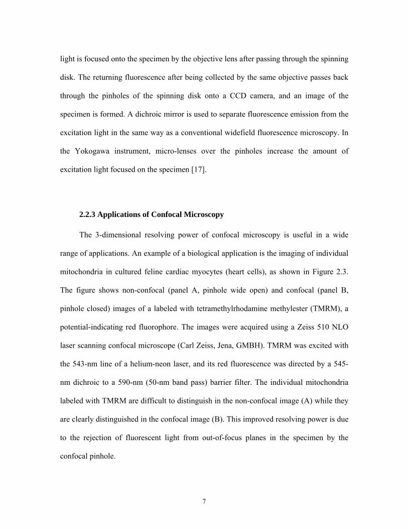
2.2.3 Applications of Confocal Microscopy

The 3-dimensional resolving power of confocal microscopy is useful in a wide

range of applications. An example of a biological application is the imaging of individual

mitochondria in cultured feline cardiac myocytes (heart cells), as shown in Figure 2.3.

The figure shows non-confocal (panel A, pinhole wide open) and confocal (panel B,

pinhole closed) images of a labeled with tetramethylrhodamine methylester (TMRM), a

potential-indicating red fluorophore. The images were acquired using a Zeiss 510 NLO

laser scanning confocal microscope (Carl Zeiss, Jena, GMBH). TMRM was excited with

the 543-nm line of a helium-neon laser, and its red fluorescence was directed by a 545-

nm dichroic to a 590-nm (50-nm band pass) barrier filter. The individual mitochondria

labeled with TMRM are difficult to distinguish in the non-confocal image (A) while they

are clearly distinguished in the confocal image (B). This improved resolving power is due

to the rejection of fluorescent light from out-of-focus planes in the specimen by the

confocal pinhole.

7

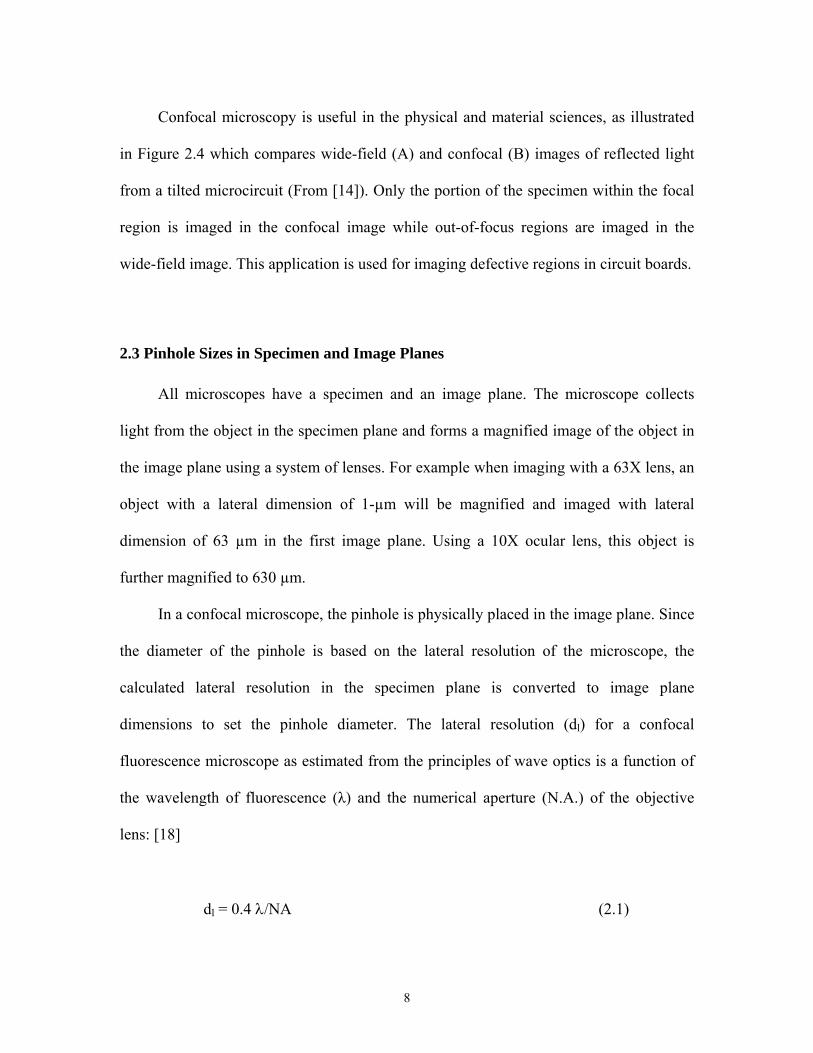
Confocal microscopy is useful in the physical and material sciences, as illustrated

in Figure 2.4 which compares wide-field (A) and confocal (B) images of reflected light

from a tilted microcircuit (From [14]). Only the portion of the specimen within the focal

region is imaged in the confocal image while out-of-focus regions are imaged in the

wide-field image. This application is used for imaging defective regions in circuit boards.

2.3 Pinhole Sizes in Specimen and Image Planes

All microscopes have a specimen and an image plane. The microscope collects

light from the object in the specimen plane and forms a magnified image of the object in

the image plane using a system of lenses. For example when imaging with a 63X lens, an

object with a lateral dimension of 1-µm will be magnified and imaged with lateral

dimension of 63 µm in the first image plane. Using a 10X ocular lens, this object is

further magnified to 630 µm.

In a confocal microscope, the pinhole is physically placed in the image plane. Since

the diameter of the pinhole is based on the lateral resolution of the microscope, the

calculated lateral resolution in the specimen plane is converted to image plane

dimensions to set the pinhole diameter. The lateral resolution (dl) for a confocal

fluorescence microscope as estimated from the principles of wave optics is a function of

the wavelength of fluorescence (λ) and the numerical aperture (N.A.) of the objective

lens: [18]

dl = 0.4 λ/NA (2.1)

8

where NA is defined from the index of refraction in the specimen plane (n) and the half

angle of the cone of light collected by the objective lens (θ):

NA = n sinθ (2.2)

The smallest resolvable point in the specimen is called an Airy disk and has a

diameter of dl. The diameter of this Airy disk as projected on the pinhole (D) is:

Dl = dl x M (2.3)

M is magnification at the pinhole image plane. The parameter Dl defines the physical size

of one Airy unit in the pinhole image plane.

For optimal depth resolution in confocal microscopy, pinhole diameter is set to one

Airy unit. Thus for a fluorescence wavelength of 500-nm, a 1.4 NA objective lens and

magnification at the pinhole plane of 63, the pinhole diameter will be set to a physical

diameter of 9 µm. Two Airy units will equate to a physical diameter of 18 µm and so

forth.

By setting the pinhole diameter to one Airy unit, the resulting axial resolution (da)

of a confocal microscope in specimen plane dimensions is: [18]

da = 1.4nλ/(NA)2 (2.4)

The resulting axial resolution for the example above is 0.6 µm.

9

For my project, I use Airy units for expressing pinhole diameters as well as pinhole

shifting distances (m) in the image plane. Thus, a one Airy unit pinhole shift (m=1) is

equals to a distance of one Airy unit pinhole diameter and hence a physical shift distance

of 9 µm for the example above. A two Airy unit pinhole shift (m=2) is a physical shift

distance of 18 µm and so forth.

Also, diameter of the laser beam at the point of focus in the specimen is determined

by using equation 2.1 but using the wavelength for excitation instead of the wavelength

of fluorescence. Because the wavelength of excitation is always smaller than the

wavelength of emission in conventional one-photon excitation fluorescence, the diameter

of the laser spot at the point of focus is actually slightly smaller than the lateral resolution

of the fluorescence imaging.

2.4 Multiphoton Excitation in Fluorescence Microscopy

In conventional fluorometry and fluorescence microscopy, a single photon excites

the fluorescent molecule. Since the excitation beam traverses the entire thickness of the

specimen, volumes of the specimen above and below the plane of focus are excited,

although fluorescence arising from these out-of-focus regions is not imaged in a confocal

fluorescence microscope. Nonetheless, photodamage and photobleaching can occur in

these regions, which can be a major concern especially when stacks of images are

collected in axial direction. A way to overcome this problem is multiphoton excitation

microscopy.

Multiphoton excitation was first proposed by Maria-Goppert Mayer in her doctoral

dissertation based on quantum chemical considerations and was first applied to biological

10

microscopy by Denk et al. [19, 20]. In contrast to conventional fluorescence in which a

single photon excites a fluorophore, in multiphoton fluorescence, two or more photons

excite the fluorophore to its excited state, as illustrated by the Jablonski diagram in

Figure 2.5. A Jablonski diagram, named after the Polish physicist Aleksander Jabłoński,

illustrates the energetic states of a molecule during transitions between different excited

states. In two-photon excitation, a first photon excites a fluorophore from the ground state

to an intermediate singlet state. A second photon striking almost simultaneously then

excites the molecule from the intermediate state to the excited singlet state. Return to the

ground state is then associated with release of energy as a fluorescence photon. Excited

states after one and two-photon excitation are essentially identical. Thus, two-photon

excitation gives rise to the same fluorescence as one-photon excitation.

For two-photon excitation to occur, photons must be absorbed within femtoseconds

of one another, since the intermediate state is very short lived. Two-photon excitation is

accomplished by using laser pulses of femto- or picosecond duration with fast repetition

rates. The excitation light is focused with a high NA lens to a small spot in the specimen

and scanned across the specimen just as in confocal microscopy. However, the relation

between instantaneous light flux and fluorescence excitation is quadratic. Namely,

fluorescence excitation increases with the square of light intensity in the specimen. Two-

photon excitation falls off as the fourth power of the distance from the focal point of the

objective in the specimen. This results in an inherent 3-D optical sectioning capability in

two-photon microscopy. Moreover, fluorescence excitation only occurs at the crossover

point of the beam, whereas in one-photon excitation fluorescence and associated

photodamage occur throughout the beam (see Figure 2.6 which shows one and two-

11

photon fluorescence emission from a solution of fluorescein [21]). Thus, in the one-

photon case fluorescence arises from planes above and below the focal point, while the

two-photon fluorescence arises essentially from only the crossover point since two

photon fluorescence intensity declines as the fourth power of the distance from crossover.

This fall off also essentially eliminates out-of-focus photobleaching and toxicity

compared to single-photon excitation [22].

Two-photon excitation uses photons of approximately twice the wavelength of

single photon excitation. Use of long wavelength red and infrared wavelengths results in

deeper tissue penetration, since light scattering inside tissue is inversely proportional to

the fourth power of the wavelength of light [21]. Moreover, red and intrared light is

poorly absorbed by biological tissues. Hence except for two-photon excitation at the in-

focus plane, virtually all the excitation light passes harmlessly through the specimen.

Applications of two-photon microscopy include imaging of brain slices, intact

embryos and other primary culture-tissue preparations. Two-photon excitation

microscopy has also been used to perform time-lapse imaging of hamster embryo

development. Another demonstration of the power of two-photon excitation microscopy

is the imaging of the naturally occurring reduced pyridine nucleotides [NAD(P)H] as an

indicator of cellular respiration [23]. Increasingly, two-photon microscopy is used for

intravital (in vivo) imaging of tissues of living animals.

2.4 Advances in Microscopy

In the past several years confocal and multiphoton microscopy has been

increasingly coupled to techniques like FLIM (fluorescence lifetime imaging

12

microscopy), FRAP (fluorescence recovery after photobleaching), and FRET

(fluorescence resonance energy transfer) to study various biological phenomena. FLIM in

particular has proved valuable for probing biological phenomena and is relatively

insensitive to artifacts introduced by fluctuations in detector gain, excitation intensity and

fluorophore redistribution.

2.5 Fluorescence Lifetime Imaging Microscopy

Conventional fluorescence microscopy uses the intensity of fluorescence to create

images for investigation of biological phenomena of interest. However, the intensity of

fluorescence depends on a variety of factors other than the biology being investigated,

such as detector gain, excitation intensity and fluorophore concentration. Fluorescence

lifetime, by contrast, is not affected by such variables, making FLIM an important

emerging technology for biologists.

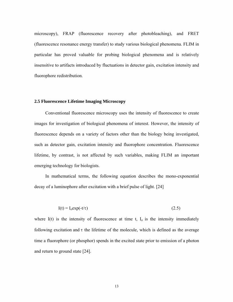
In mathematical terms, the following equation describes the mono-exponential

decay of a luminophore after excitation with a brief pulse of light. [24]

I(t) = Ioexp(-t/τ) (2.5)

where I(t) is the intensity of fluorescence at time t, Io is the intensity immediately

following excitation and τ the lifetime of the molecule, which is defined as the average

time a fluorophore (or phosphor) spends in the excited state prior to emission of a photon

and return to ground state [24].

13

For a population of excited fluorophores, 63% of the excited molecules relax to

ground state during one lifetime of the fluorophore. Thus, 37% remain in the excited

state. Fluorescence lifetime is determined experimentally by measuring the time taken for

the fluorescence intensity to decrease to 37% of its initial value after excitation with a

brief pulse of light (Figure 2.7). By combining lifetime measurements with fluorescent

wide-field or confocal microscopy, one can perform FLIM.

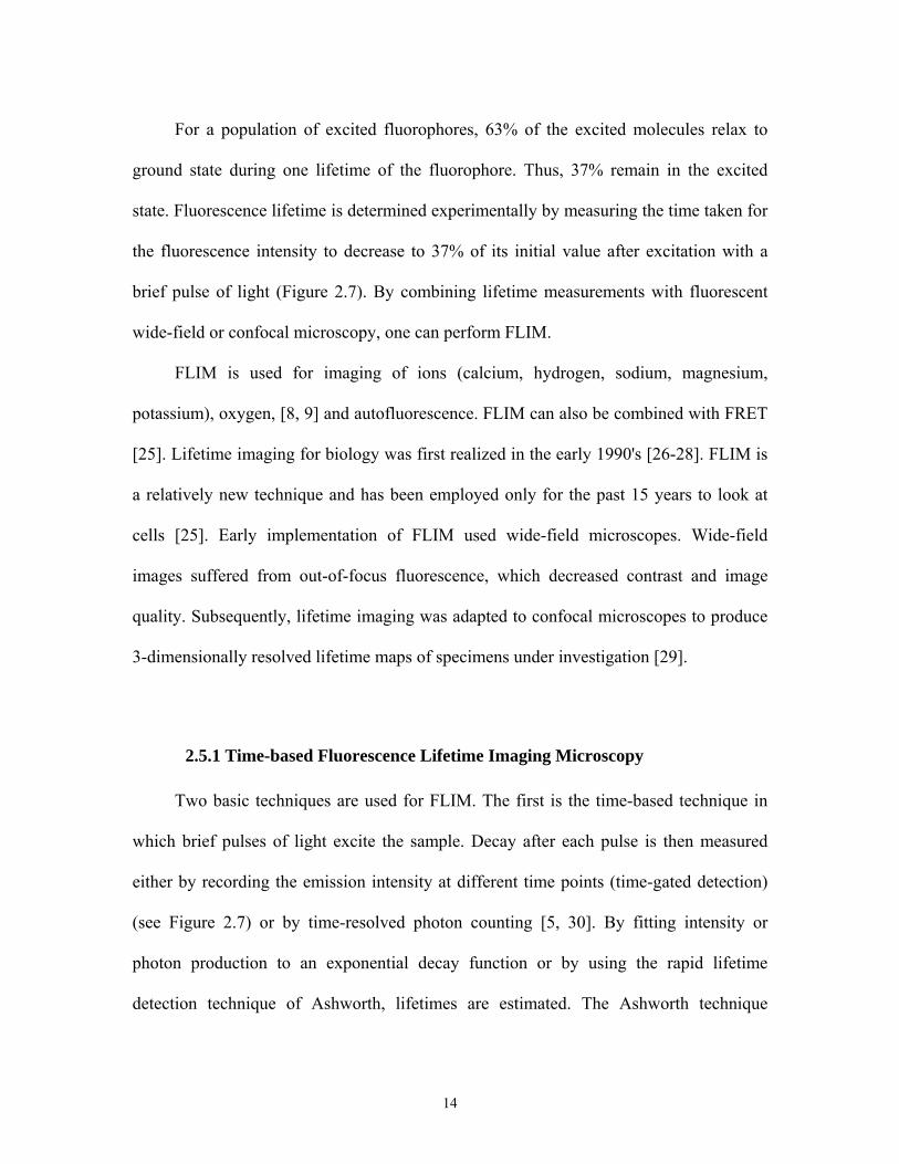
FLIM is used for imaging of ions (calcium, hydrogen, sodium, magnesium,

potassium), oxygen, [8, 9] and autofluorescence. FLIM can also be combined with FRET

[25]. Lifetime imaging for biology was first realized in the early 1990's [26-28]. FLIM is

a relatively new technique and has been employed only for the past 15 years to look at

cells [25]. Early implementation of FLIM used wide-field microscopes. Wide-field

images suffered from out-of-focus fluorescence, which decreased contrast and image

quality. Subsequently, lifetime imaging was adapted to confocal microscopes to produce

3-dimensionally resolved lifetime maps of specimens under investigation [29].

2.5.1 Time-based Fluorescence Lifetime Imaging Microscopy

Two basic techniques are used for FLIM. The first is the time-based technique in

which brief pulses of light excite the sample. Decay after each pulse is then measured

either by recording the emission intensity at different time points (time-gated detection)

(see Figure 2.7) or by time-resolved photon counting [5, 30]. By fitting intensity or

photon production to an exponential decay function or by using the rapid lifetime

detection technique of Ashworth, lifetimes are estimated. The Ashworth technique

14

involves measuring the photon intensity under different regions of the decay and use the

intensities to calculate the lifetime [31].

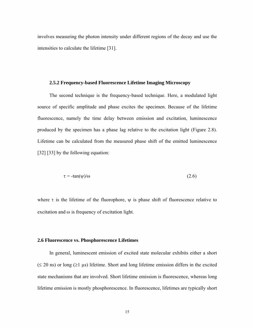
2.5.2 Frequency-based Fluorescence Lifetime Imaging Microscopy

The second technique is the frequency-based technique. Here, a modulated light

source of specific amplitude and phase excites the specimen. Because of the lifetime

fluorescence, namely the time delay between emission and excitation, luminescence

produced by the specimen has a phase lag relative to the excitation light (Figure 2.8).

Lifetime can be calculated from the measured phase shift of the emitted luminescence

[32] [33] by the following equation:

τ = -tan(ψ)/ω (2.6)

where τ is the lifetime of the fluorophore, ψ is phase shift of fluorescence relative to

excitation and ω is frequency of excitation light.

2.6 Fluorescence vs. Phosphorescence Lifetimes

In general, luminescent emission of excited state molecular exhibits either a short

(≤ 20 ns) or long (≥1 µs) lifetime. Short and long lifetime emission differs in the excited

state mechanisms that are involved. Short lifetime emission is fluorescence, whereas long

lifetime emission is mostly phosphorescence. In fluorescence, lifetimes are typically short

15

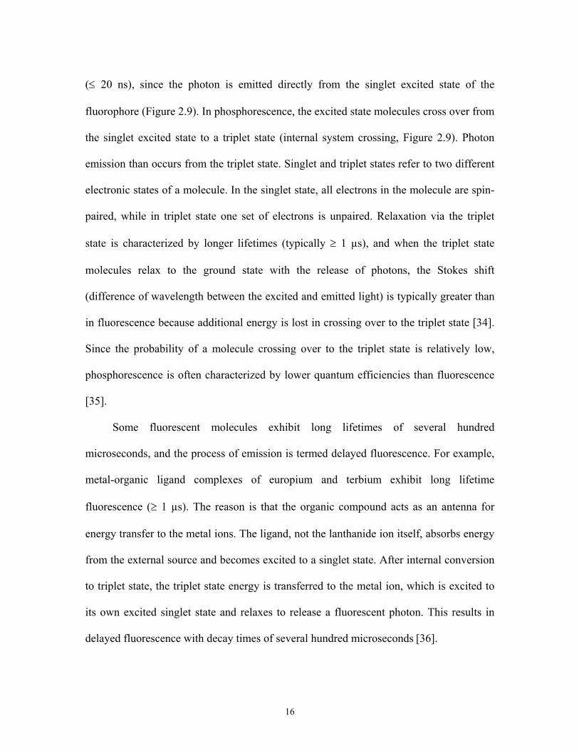
(≤ 20 ns), since the photon is emitted directly from the singlet excited state of the

fluorophore (Figure 2.9). In phosphorescence, the excited state molecules cross over from

the singlet excited state to a triplet state (internal system crossing, Figure 2.9). Photon

emission than occurs from the triplet state. Singlet and triplet states refer to two different

electronic states of a molecule. In the singlet state, all electrons in the molecule are spin-

paired, while in triplet state one set of electrons is unpaired. Relaxation via the triplet

state is characterized by longer lifetimes (typically ≥ 1 µs), and when the triplet state

molecules relax to the ground state with the release of photons, the Stokes shift

(difference of wavelength between the excited and emitted light) is typically greater than

in fluorescence because additional energy is lost in crossing over to the triplet state [34].

Since the probability of a molecule crossing over to the triplet state is relatively low,

phosphorescence is often characterized by lower quantum efficiencies than fluorescence

[35].

Some fluorescent molecules exhibit long lifetimes of several hundred

microseconds, and the process of emission is termed delayed fluorescence. For example,

metal-organic ligand complexes of europium and terbium exhibit long lifetime

fluorescence (≥ 1 µs). The reason is that the organic compound acts as an antenna for

energy transfer to the metal ions. The ligand, not the lanthanide ion itself, absorbs energy

from the external source and becomes excited to a singlet state. After internal conversion

to triplet state, the triplet state energy is transferred to the metal ion, which is excited to

its own excited singlet state and relaxes to release a fluorescent photon. This results in

delayed fluorescence with decay times of several hundred microseconds [36].

16

The point of transition of short lifetime to long lifetime luminescence is not clearly

defined in literature and is more often defined in reference to the suitability of different

instruments to make the lifetime measurements. For my dissertation work, I use the term

short lifetime luminescence to describe fluorescence lifetimes of less than 20 ns and long

lifetime luminescence for delayed fluorescence or phosphorescence with lifetimes of

greater than 1 µs.

2.7 Oxygen Sensing Techniques

Techniques for sensing oxygen at the tissue and cellular levels include

microsphectrophotometry, redox fluoromerty, oxygen-sensitive electrodes, MRI and

phosphorescence-based oxygen-sensing.

2.7.1 Microsphectrophotometry

Measurements of oxygen in single cardiac myocytes and in myocardial tissue is

performed using myoglobin microsphectrophotometry [37, 38, 39]. This technique works

by using two wavelengths of light. The two wavelengths are absorbed by hemoglobin by

amounts which differ depending on whether the hemoglobin is saturated or desaturated

with oxygen. In the red wavelength, oxygen saturated hemoglobin absorbs less light than

hemoglobin, while the reverse occurs at the infrared wavelength. By calculating the

absorption at the two wavelengths one can compute the proportion of hemoglobin that is

oxygenated.

17

2.7.2 Redox Fluorometry

An indirect technique to measure oxygen at cellular level is by monitoring the

fluorescence from pyridine nucleotides [38, 39, 40]. The bound and free intracellular

reduced pyridine nucleotides (NADH and NADPH) are fluorescent at 450-nm on

excitation at 366-nm. The intensity of NADH fluorescence depends on the tissue

oxygenation level. An increase in the pyridine nucleotide fluorescence is equated with a

decrease in tissue oxygenation.

2.7.3 Oxygen Electrodes

Another technique to measure oxygen employs oxygen electrodes. An oxygen

electrode is a specialized form of electrochemical cell which consists of two electrodes

immersed in an electrolyte solution. Application of a polarizing voltage across the two

electrodes, a platinum cathode and a Ag/AgCl anode, results in the flow of current

through the electrode whose magnitude is proportional to the amount of dissolved oxygen

in the electrolyte and hence the surrounding media [38]. Oxygen is reduced at the

platinum cathode, and the electrolyte enables the current to flow whose magnitude is

proportional to the oxygen concentration. Such an electrode system was first developed

by Clark to measure oxygen in blood samples and hence also called Clark style electrode.

A self-referencing oxygen microelectrode developed by Land et al. [39] enables the

continuous measurement of oxygen concentration from distinct regions next to the

plasma membrane around a single cell. This non-invasive technique measures oxygen

flux around single cells by the translational movement of a Whalen-type oxygen-selective

18

polarographic microelectrode (2-3 µm tip diameter) through the oxygen gradient within

the unstirred layer next to the cell membrane [39].

2.7.4 Functional Magnetic Resonance Imaging

Functional magnetic resonance imaging (fMRI) uses MRI to measure the oxygen

levels in tissues. The magnetic resonance (MR) signal of tissues depends on the level of

blood oxygenation. Hemoglobin is diamagnetic when oxygenated but paramagnetic when

deoxygenated. The magnetic resonance (MR) signal of tissues is therefore different

depending on the level of oxygenation. These differential signals can be detected using an

appropriate MR pulse sequence as blood oxygenation contrast. Changes in MRI signals

can be correlated to changes in tissue oxygen consumption [40]. However, MRI

techniques have a resolution in the millimeter scale thus lacking the ability to measure

cellular level oxygen concentrations.

2.7.5 Luminescence Based Oxygen Sensing

Luminescence based techniques are well suited for non invasive oxygen imaging of

cells with micron resolution. With a suitable light source to excite an oxygen sensitive

luminophore, fluorescence or phosphorescence intensity and lifetime depend on oxygen

concentration. Oxygen quenches various luminophores in the excited state, thereby

transferring the energy of the excited singlet or triplet state to form excited state singlet

oxygen as the luminophore relaxes to ground state without the release of a photon (Figure

2.10). Thus, the reaction of oxygen with the excited state luminophore is competing with

19

luminescence decay of the excited state to the ground state. Changes in intensity and

lifetime of the luminophore are markers of the changes in oxygen concentration. The

longer the lifetime of the luminophore the greater is the probability of the excited state

molecule being quenched by oxygen. Hence, luminophores with lifetimes ranging from

one to several hundred microseconds are preferred for such oxygen measurements.

The oxygen dependent change in the intensity of luminescence is characterized by

the Stern-Volmer relation:

τo/τ = Io/I = 1 + kqτo [O2]p (2.7)

where τo and Io are the lifetime and intensity of the luminophore in the absence of

oxygen; τ and I are the lifetime and intensity at the given oxygen concentration; kq is the

quenching constant and [O2]p is the partial pressure of oxygen.

According to this relation, the ratio of the lifetime or intensity of the probe at zero

oxygen to that at given oxygen concentration is a function of the quenching constant, the

lifetime at oxygen and oxygen concentration. The equation can be rearranged to solve for

oxygen:

[O2]p = (1/τ - 1/τo)1/kq (2.8)

[O2]p = (1/Ι- 1/Ιo)1/kq (2.9)

Thus, one can measure oxygen concentration from measurements of lifetime and

knowledge of the quenching constant and lifetime in the absence of oxygen. Most work

20

measuring oxygen using luminescence makes use of luminescent probes like Ru(II) and

Os(II) -diimine complexes and Pt(II)/Pd(II) porphyrin complexes that are characterized

by long lifetimes typically from hundreds of nanoseconds to hundreds of microseconds

[12, 34, 41, 42, 43, 44, 45].

2.8 Mitochondrial Metabolism

As cardiac output increases, ATP production by oxidative phosphorylation must

respond within seconds to avoid large fluctuations of myocardial ATP and creatine

phosphate which would otherwise lead to contractile dysfunction. Changes of

intramitochondrial Ca2+ has been proposed to regulate mitochondrial oxidative

metabolism in response to the rapid changes in cardiac energy demand [41, 42].

Specifically, increases of intramitochondrial Ca2+ has been proposed to activate

dehydrogenases, adenine nucleotide translocation and ATP synthase activity [43, 44, 45]

Confocal microscopy reveals that changes in mitochondrial free Ca2+ mediated by

the ruthenium red sensitive mitochondrial calcium uniporter occur on a beat-to-beat basis

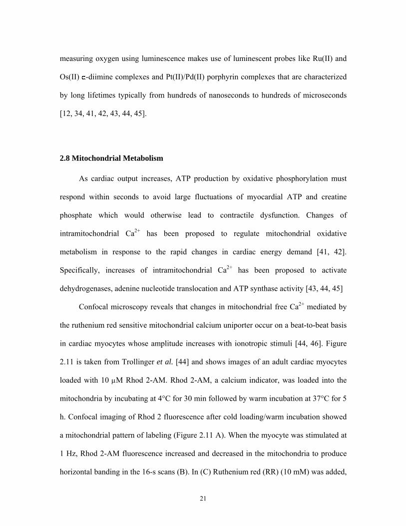
in cardiac myocytes whose amplitude increases with ionotropic stimuli [44, 46]. Figure

2.11 is taken from Trollinger et al. [44] and shows images of an adult cardiac myocytes

loaded with 10 μM Rhod 2-AM. Rhod 2-AM, a calcium indicator, was loaded into the

mitochondria by incubating at 4°C for 30 min followed by warm incubation at 37°C for 5

h. Confocal imaging of Rhod 2 fluorescence after cold loading/warm incubation showed

a mitochondrial pattern of labeling (Figure 2.11 A). When the myocyte was stimulated at

1 Hz, Rhod 2-AM fluorescence increased and decreased in the mitochondria to produce

horizontal banding in the 16-s scans (B). In (C) Ruthenium red (RR) (10 mM) was added,

21

and another confocal image was collected after 20 min. In the presence of ruthenium red,

mitochondrial Ca2+ transients were suppressed.

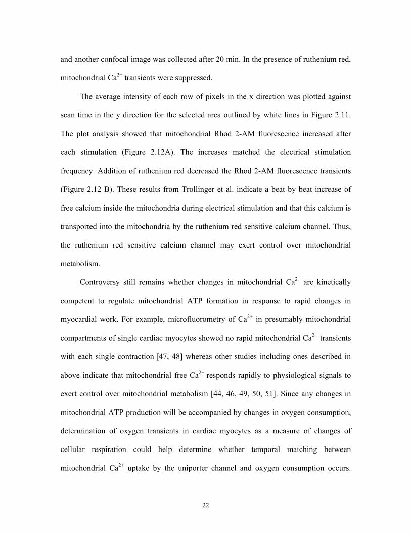
The average intensity of each row of pixels in the x direction was plotted against

scan time in the y direction for the selected area outlined by white lines in Figure 2.11.

The plot analysis showed that mitochondrial Rhod 2-AM fluorescence increased after

each stimulation (Figure 2.12A). The increases matched the electrical stimulation

frequency. Addition of ruthenium red decreased the Rhod 2-AM fluorescence transients

(Figure 2.12 B). These results from Trollinger et al. indicate a beat by beat increase of

free calcium inside the mitochondria during electrical stimulation and that this calcium is

transported into the mitochondria by the ruthenium red sensitive calcium channel. Thus,

the ruthenium red sensitive calcium channel may exert control over mitochondrial

metabolism.

Controversy still remains whether changes in mitochondrial Ca2+ are kinetically

competent to regulate mitochondrial ATP formation in response to rapid changes in

myocardial work. For example, microfluorometry of Ca2+ in presumably mitochondrial

compartments of single cardiac myocytes showed no rapid mitochondrial Ca2+ transients

with each single contraction [47, 48] whereas other studies including ones described in

above indicate that mitochondrial free Ca2+ responds rapidly to physiological signals to

exert control over mitochondrial metabolism [44, 46, 49, 50, 51]. Since any changes in

mitochondrial ATP production will be accompanied by changes in oxygen consumption,

determination of oxygen transients in cardiac myocytes as a measure of changes of

cellular respiration could help determine whether temporal matching between

mitochondrial Ca2+ uptake by the uniporter channel and oxygen consumption occurs.

22

While techniques to measure the calcium transients have been developed previously [44,

46], oxygen sensing in single cells with both spatial and temporal resolution has not been

previously demonstrated.

2.9 Aims of Project

The primary goal of this project was to develop a new technique for lifetime

imaging of long lifetime phosphors and other luminophores by adaptation of a

confocal/multiphoton microscope. Existing commercial instruments for lifetime imaging

are specialized, expensive and generally unsuitable for lifetime imaging of long lifetime

probes. Here, I develop an inexpensive technique to adapt a standard laser scanning

confocal microscope for lifetime imaging of phosphors. Any new technology needs

applications to justify its development. Thus, the secondary goal of this project was to

apply the new technology to a biological application.

A long standing debate in biology is the regulation of mitochondrial oxidative

phosphorylation by mitochondrial calcium transients. By measuring oxygen

simultaneously with calcium one can add further evidence to the regulation of

mitochondrial metabolism by calcium. Therefore a final goal of this project was to

demonstrate the use of LLIM-CPS to measure oxygen at the cellular level and to show

the possibility of using this technique to measure oxygen with calcium.

My Specific Aims were:

23

1. Luminescence lifetime imaging by pinhole shifting of a confocal microscope

(LLIM-CPS)

Specific Aim 1 is to develop a method to adapt a standard laser scanning

confocal/multiphoton microscope to perform time-domain based lifetime imaging by using

the principle of pinhole shifting to capture delayed (long lifetime) luminescence.

Experimental validation of theory will be performed by imaging luminophores with

different lifetimes.

2. Measurement of lifetime of europium using LLIM-CPS

In Specific Aim 2, I will show how to use the adapted microscope to measure

lifetimes. Using this technique I will measure lifetime of long lifetime europium

microspheres, which have a lifetime of several hundred microseconds.

3. Optimization of pinhole diameter, position and laser dwell times for LLIM-CPS

In order to measure lifetimes accurately, instrumental settings, such as pinhole

diameter, position and laser dwell times, of the confocal microscope require optimization.

Accordingly, theory to optimize these settings will be developed and assessed

experimentally.

4. Measurement of the lifetime and intensity of oxygen sensitive luminophore using

LLIM-CPS

24

Using LLIM-CPS, I will quantify the oxygen dependent lifetime and intensity of long

lifetime oxygen probe tris-4, 7 diphenyl 1, 10-phenanthrolin ruthenium (II) complex

(TDPR) and Pd-meso-tetra-(4-carboxyphenyl) tetrabenzoporphyrin (Oxyphor G2).

5. Application of LLIM-CPS to Study Oxygen in Myocytes

As a biological application, LLIM-CPS will be used to measure oxygen in adult

cardiac myocytes cells. This will include selection of suitable long lifetime oxygen

sensing luminophore, optimization of luminophore and its application for sensing oxygen

in myocytes.

2.10 Novelty of Project

The literature on measuring oxygen in single myocytes with lifetime imaging and

confocal/multiphoton microscopy is very limited. A PubMed search with the keywords

lifetime imaging and myocytes reveals only one relevant paper, and a search on lifetime

imaging and cellular oxygen yields no hits. Indeed, lifetime imaging with confocal and

multiphoton imaging yields only 22 hits. The reasons for such few hits include the very

recent development of lifetime imaging by confocal/multiphoton microscopy and the

difficulty and expertise required for implementing the new technology. Moreover, most

technologies for measuring lifetimes are designed for measuring lifetimes in the pico- and

nanosecond time scale and are unsuitable for measuring lifetimes in the microsecond

range required for oxygen-sensing phosphors. No methods have been published that

allow lifetime imaging of such long lifetime luminophores using a confocal microscope

with pinhole shifting.

25

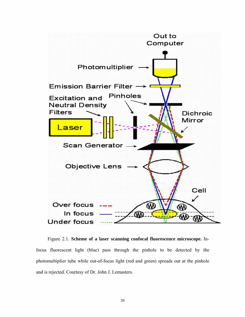
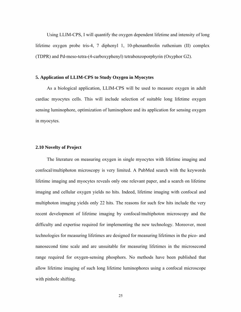
Figure 2.1. Scheme of a laser scanning confocal fluorescence microscope. In-

focus fluorescent light (blue) pass through the pinhole to be detected by the

photomultiplier tube while out-of-focus light (red and green) spreads out at the pinhole

and is rejected. Courtesy of Dr. John J. Lemasters.

26

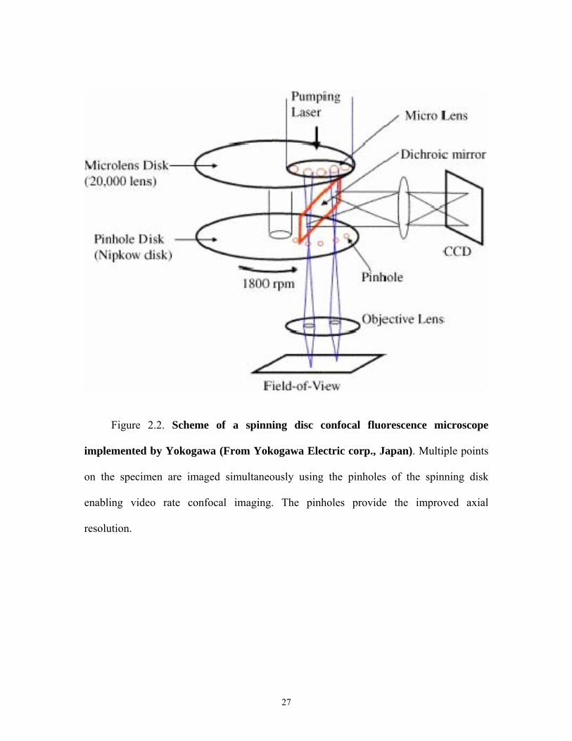
Figure 2.2. Scheme of a spinning disc confocal fluorescence microscope

implemented by Yokogawa (From Yokogawa Electric corp., Japan). Multiple points

on the specimen are imaged simultaneously using the pinholes of the spinning disk

enabling video rate confocal imaging. The pinholes provide the improved axial

resolution.

27

Figure 2.3. Non-confocal (A) and confocal with pinhole closed (B) images of

cultured myocytes labeled with TMRM. The mitochondria are better distinguished in

the confocal image in A compared to the non-confocal image in B. The images were

acquired using a Zeiss LSM 510 NLO META confocal microscope.

28

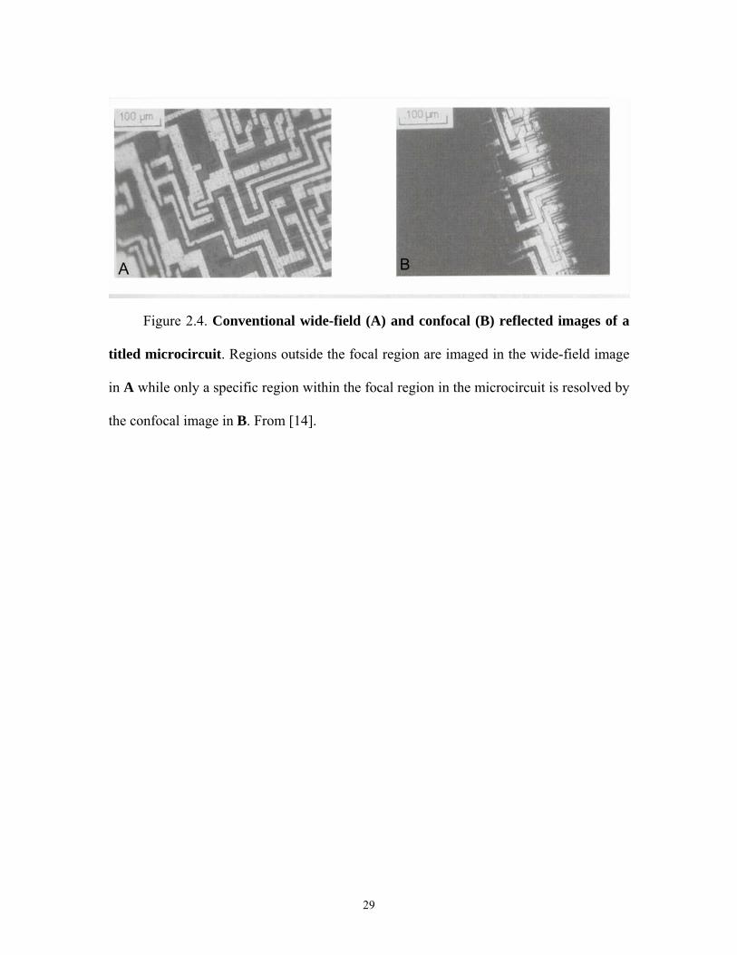
Figure 2.4. Conventional wide-field (A) and confocal (B) reflected images of a

titled microcircuit. Regions outside the focal region are imaged in the wide-field image

in A while only a specific region within the focal region in the microcircuit is resolved by

the confocal image in B. From [14].

29

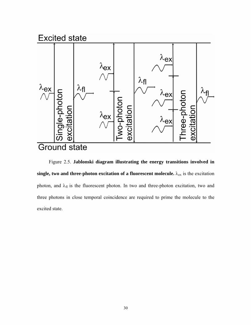
Figure 2.5. Jablonski diagram illustrating the energy transitions involved in

single, two and three-photon excitation of a fluorescent molecule. λex is the excitation

photon, and λfl is the fluorescent photon. In two and three-photon excitation, two and

three photons in close temporal coincidence are required to prime the molecule to the

excited state.

30

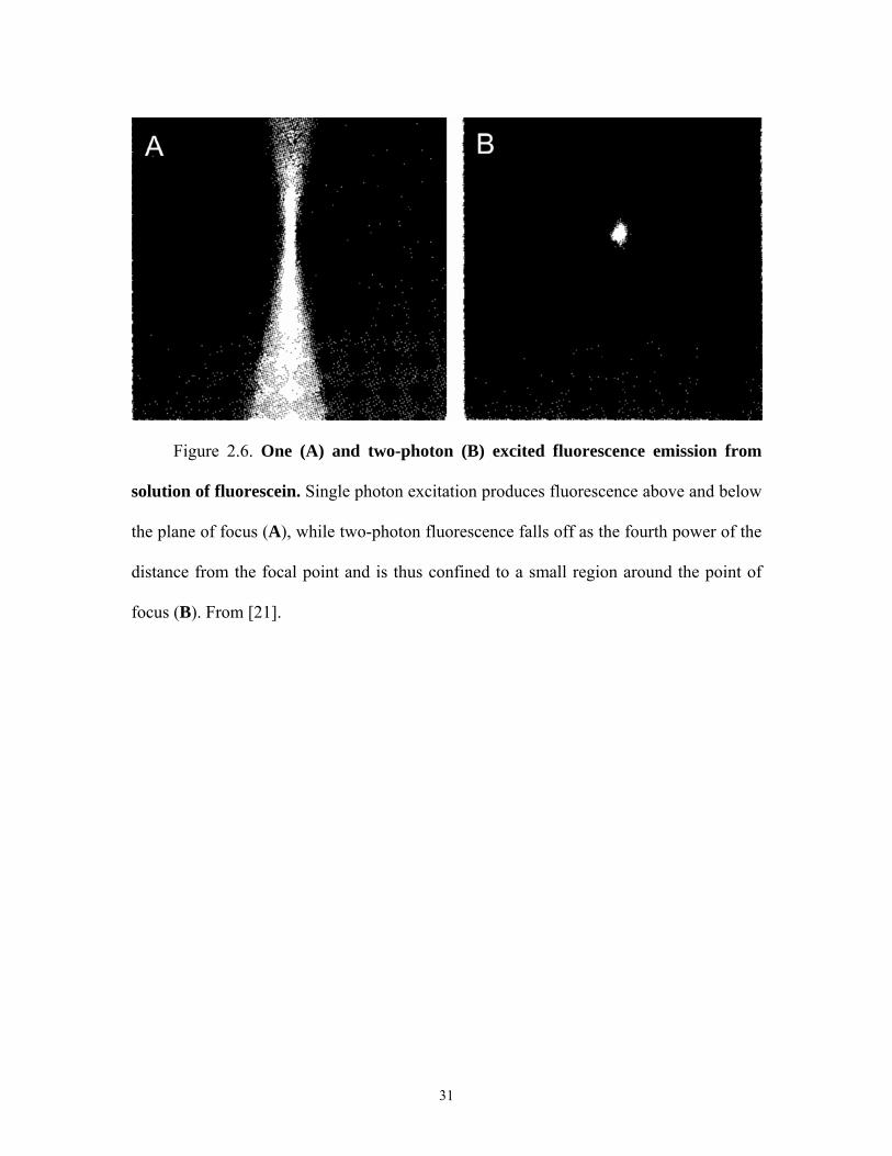
Figure 2.6. One (A) and two-photon (B) excited fluorescence emission from

solution of fluorescein. Single photon excitation produces fluorescence above and below

the plane of focus (A), while two-photon fluorescence falls off as the fourth power of the

distance from the focal point and is thus confined to a small region around the point of

focus (B). From [21].

31

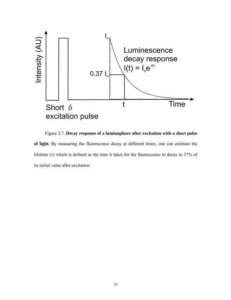
Figure 2.7. Decay response of a luminophore after excitation with a short pulse

of light. By measuring the fluorescence decay at different times, one can estimate the

lifetime (τ) which is defined as the time it takes for the fluorescence to decay to 37% of

its initial value after excitation.

32

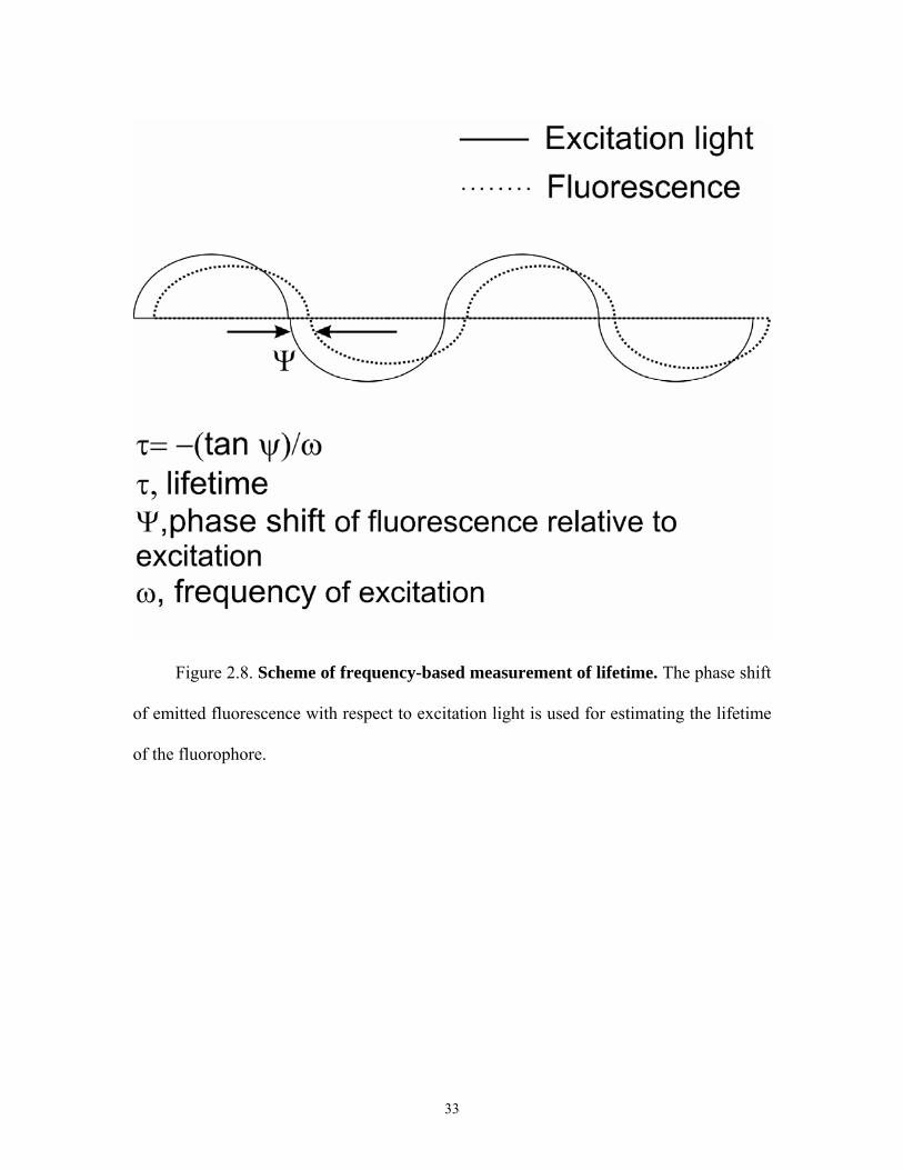
Figure 2.8. Scheme of frequency-based measurement of lifetime. The phase shift

of emitted fluorescence with respect to excitation light is used for estimating the lifetime

of the fluorophore.

33

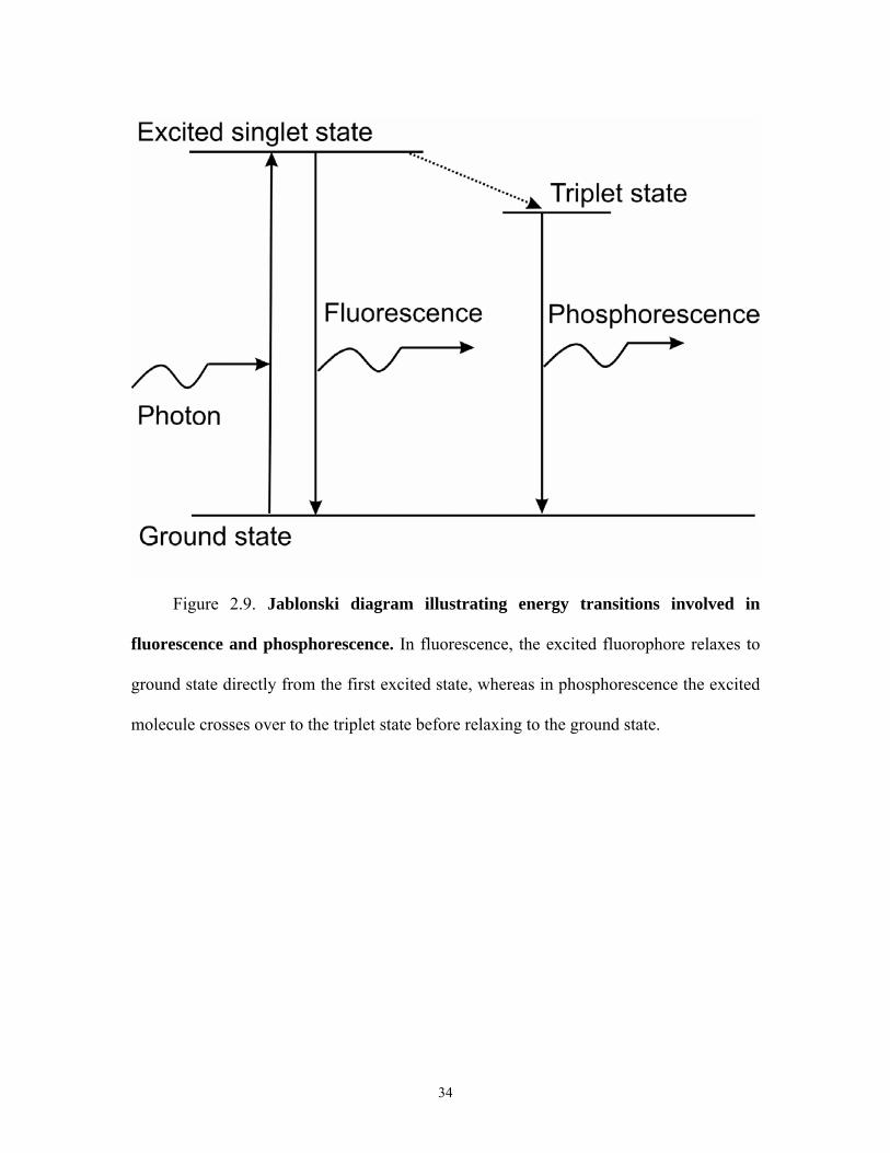
Figure 2.9. Jablonski diagram illustrating energy transitions involved in

fluorescence and phosphorescence. In fluorescence, the excited fluorophore relaxes to

ground state directly from the first excited state, whereas in phosphorescence the excited

molecule crosses over to the triplet state before relaxing to the ground state.

34

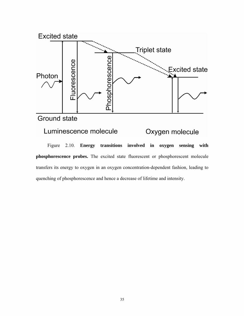
Figure 2.10. Energy transitions involved in oxygen sensing with

phosphorescence probes. The excited state fluorescent or phosphorescent molecule

transfers its energy to oxygen in an oxygen concentration-dependent fashion, leading to

quenching of phosphorescence and hence a decrease of lifetime and intensity.

35

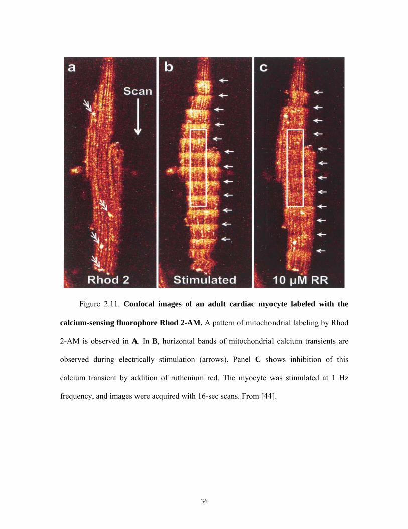
Figure 2.11. Confocal images of an adult cardiac myocyte labeled with the

calcium-sensing fluorophore Rhod 2-AM. A pattern of mitochondrial labeling by Rhod

2-AM is observed in A. In B, horizontal bands of mitochondrial calcium transients are

observed during electrically stimulation (arrows). Panel C shows inhibition of this

calcium transient by addition of ruthenium red. The myocyte was stimulated at 1 Hz

frequency, and images were acquired with 16-sec scans. From [44].

36

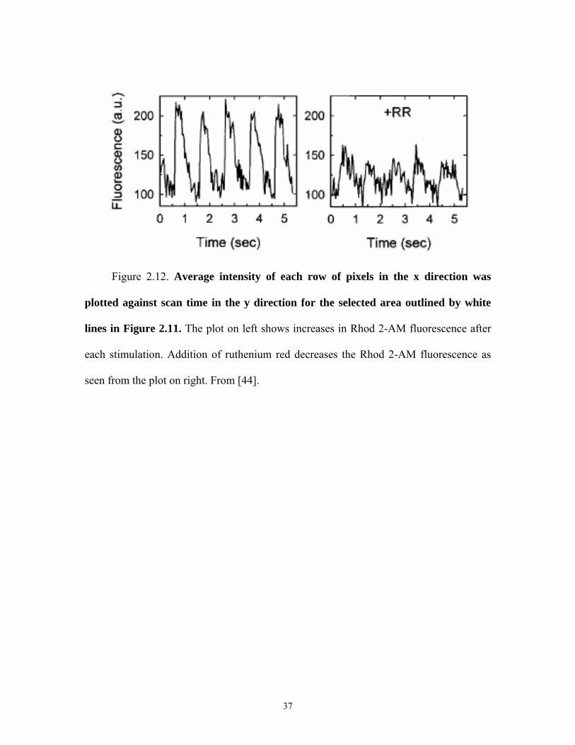
Figure 2.12. Average intensity of each row of pixels in the x direction was

plotted against scan time in the y direction for the selected area outlined by white

lines in Figure 2.11. The plot on left shows increases in Rhod 2-AM fluorescence after

each stimulation. Addition of ruthenium red decreases the Rhod 2-AM fluorescence as

seen from the plot on right. From [44].

37

CHAPTER 3

METHODS AND MATERIALS

3.1 Imaging of Long Lifetime Europium Microspheres and Short Lifetime

Luminophores

Imaging was performed with a Zeiss LSM 510 META confocal microscope (Carl

Zeiss, GmbH) equipped with internal Argon (Ar) and Helium-Neon (He-Ne) lasers and a

Coherent femtosecond pulsed Ti-Sapphire laser for multiphoton excitation (Mira900 or

Chameleon Ultra, Coherent, CA). Unless otherwise indicated, images were collected

using a 63X 1.4 NA planapochromat oil immersion lens with pinhole size set to one Airy

unit diameter as appropriate for the wavelength of fluoresced light. Pinhole shifting was

accomplished with Zeiss LSM software. Images were collected as 512 x 512 pixel scans

at 8-bit intensity resolution. Laser intensity and detector gain were adjusted such that

virtually all pixels in individual images had intensity values between 1 and 254 to avoid

over- and undersaturation. Background images were obtained by focusing the objective

lens within the coverslip and acquiring an image with the laser and detector setting the

same as used for the specimen.

Two-photon excitation of long lifetime europium microspheres (1-µm diameter),

green microspheres, rhodamine and fluorescein in solution was accomplished using 720-

nm light from the Ti-Sapphire laser. Green and red luminescence was divided by a 545-

nm long-pass dichroic and directed to photomultipliers through 525-nm (50-nm

bandpass) and 590-nm (50-nm bandpass) barrier filters, respectively. Images were

acquired at room temperature.

3.2 Imaging of Europium and Blue Microspheres

In some experiments, 1 µm diameter long lifetime europium microsphere were

imaged simultaneously with 1 µm diameter short lifetime blue microspheres. Excitation

was performed at 720-nm from the multiphoton Ti-Sapphire laser. Red and blue

luminescences were separated by a 545-nm long-pass dichroic mirror and directed to

photomultipliers through a 590-nm (50-nm bandpass) and 500-nm (20-nm bandpass)

barrier filters, respectively. Images were acquired at room temperature.

3.3 Europium Slide preparation

Solutions (5 µl) of 1-µm diameter europium (1 x 107 microspheres/µL) and green

or blue microspheres (3.6 x 107 microspheres/µL) and/or fluorescein or rhodamine (16

mM concentration) were added to 200 µl glycomethacrylate. The microsphere solutions

were sonicated for 30 min before addition to glycomethacrylate. This solution (50 µl)

was pipetted on a glass slide and covered with a 0.17 mm thickness glass coverslip. The

glass slide was the placed under UV light at 4oC for 30 min. At this point the slides were

stored at room temperature for experimentation.

39

3.4 Imaging of Oxygen Sensing Luminophores

Tris-4, 7 diphenyl 1, 10-phenanthroline ruthenium (TDPR) and Pd-meso-tetra-(4-

carboxyphenyl) tetrabenzoporphyrin (Oxyphor G2) were excited by the 488-nm Ar laser

line and the 633-nm He-Ne line, respectively. Luminescence from TDPR and Oxyphor

G2 were imaged through 600-nm (50-nm bandpass) and 700-nm (50-nm band pass)

barrier filters, respectively. The oxygen sensing luminophores were imaged on a glass

coverslip placed inside a closed incubation chamber with ports for perfusion (POC-R Cell

Cultivation System, PeCon, GmbH). The closed chamber was placed inside the

microscope incubation system (PeCon, GmbH) on the microscope stage, and images

were acquired. Oxygen was varied by perfusing KRH (Krebs-Ringer-HEPES buffer)

containing oxyrase. Images were acquired at 37°C.

3.5 Imaging PtTBP-AG2-PEG

To image oxygen-sensing PtTBP-AG2-PEG, the phosphor was excited with the

633-nm line of a He-Ne laser, and phosphorescence was directed to a photomultiplier

tube through a 545-nm dichroic mirror and a 690-nm long pass filter. Images were

acquired at 37°C.

3.6 Myocyte Isolation

Adult feline cardiac myocytes were the generous gift of Dr. Donald Menick.

Briefly, ventricular myocytes were isolated by collagenase digestion [52] and attached to

laminin-coated coverslips (0.17 mm thickness) on the bottom of 35-mm diameter Petri

40

dishes (MatTek Corporation, Ashland, MA). Myocytes were incubated at 37°C in 5%

CO2/air for 12 to 16 h in nutrient medium (1:1 mix of medium 199 and Joklik's medium

supplemented with 0.05 U/ml insulin, 1 mM creatine, 1 mM octanoic acid, 1 mM taurine,

10 U/ml pencillin and 10 mg/ml streptomycin).

3.7 Tetramethylrhodamine Methylester Labeling

Myocytes were loaded with 200 nM tetramethylrhodamine methylester (TMRM)

for 30 minutes at 37oC in KRH (Krebs-Ringer-HEPES buffer [KRH]: 110 mM NaCl, 5.0

mM KCl, 1.25 mM CaCl2, 0.5 mM Na2HPO4, 0.5 mM KH2PO4, 1.0 mM MgSO4, 10 mM

glucose, 1.0 mM octanoic acid, and 20 mM HEPES and 10 mM glucose). When the

medium was changed after TMRM loading, TMRM (50 nM) was added to maintain

equilibrium distribution of the fluorophore.

3.8 Myocyte Imaging with Tetramethylrhodamine Methylester and PtTBP-AG2-

PEG

Images of myocytes loaded with 200 nM TMRM were collected at 37°C with a

Zeiss 510 laser scanning confocal microscope in the prescence of oxygen sensing

luminophores PtTBP-AG2-PEG (100 µM). TMRM and PtTBP-AG2-PEG fluorescence

were excited, respectively, with the 543- and 633-nm lines of a He-Ne laser.

Luminescences from TMRM and PtTBP-AG2-PEG were directed to different

photomultiplier tubes by a 545-nm long-pass dichroic through 590-nm (50-nm bandpass)

and 690-nm long pass barrier filters respectively.

41

3.9 Agarose for Covering Myocytes

Cultured myocytes were embedded with low melting point agarose to limit oxygen

diffusion. Deionised distilled water (1.8 ml) was heated to 37oC 1.5% agarose (1:1 mix of

SeaPrep and SeaKeam agarose, Cambrex Bio Science Rockland Inc., Rockland, ME) was

added. Heating continued until the solution reached a temperature of 90oC. After cooling

to 50oC, 0.2 ml of 10x KRH media and any fluorescent luminophores were added. After

cooling to 40oC, 200-300 µl of the agarose solution was poured immediately into 35-mm

diameter MatTek dishes containing myocytes in culture medium. Just prior to pouring the

agarose the culture medium was aspirated from the dish.

3.10 Software

Images were pseudocolored using the black body look-up table of Photoshop

(Adobe Systems, San Jose, CA). Intensity for images was determined using Zeiss LSM

software (Carl Zeiss, GmBH) and Photoshop. Plotting of graphs was performed using

SigmaPlot (Systat Software Inc., San Jose, CA). All illustrations were made in Corel

Draw (Corel Corporation, Eden Prairie, MN).

3.11 Luminophores and Chemicals

Europium, green and blue luminescent microspheres (1-µm diameter size) and

TMRM were obtained from Invitrogen (Carlsbad, CA). Fluorescein and rhodamine 123

were obtained from Sigma Corp. (St Louis, MO), Oxyphor G2 from Oxygen Enterprise

and TDPR from Polestar Technologies (MA). PtTBP-AG2-PEG was the kind gift from

42

Dr. Sergei A. Vinogradov at University of Pennsylvania. Oxyrase was purchased from

Oxyrase Inc. (Manchester, Ohio). Glycomethacrylate was purchased from Electron

Microscopy Sciences (Electron Microscopy Sciences, Hatfield, PA). Laminin (BD

MatrigelTM Matrix) was purchased from BD Biosceinces (BD Biosceinces, Bedford,

MA). All other chemicals and media were purchased from Invitrogen and Sigma Corp.

43

CHAPTER 4

RESULTS

4.1 Phosphorescence Lifetime Imaging Microscopy by Confocal Pinhole Shifting

In confocal microscopy, the detection pinhole is positioned to collect light exactly

from the position within the specimen over which the laser crossover spot is being

scanned (Figure 4.1). Indeed, when the pinhole is misaligned in the leading, lagging or

orthogonal directions, collection of reflected light and short lifetime luminescence drops

profoundly. However as shown in Figure 4.1, when the pinhole is shifted in the lagging

direction, delayed luminescence, namely long lifetime luminescence should be

selectively transmitted through the pinhole with rejection of short lifetime fluorescence.

The lifetimes collected depend on the distance of pinhole shifting and the speed of the

rasting laser beam across the specimen. Raster speed is inversely proportional to dwell

time, which is defined as the amount of time the laser beam resides over each pixel of the

image collected from the specimen.

The lifetimes collected for different pinhole shifts are given by:

(m-1)Δt ≤ τcollected ≤mΔt (4.1)

where m is pinhole shift in Airy units (m ≥1), Δt is dwell time of the laser spot, and

τcollected is the lifetimes collected. For a commercial laser scanning confocal microscope,

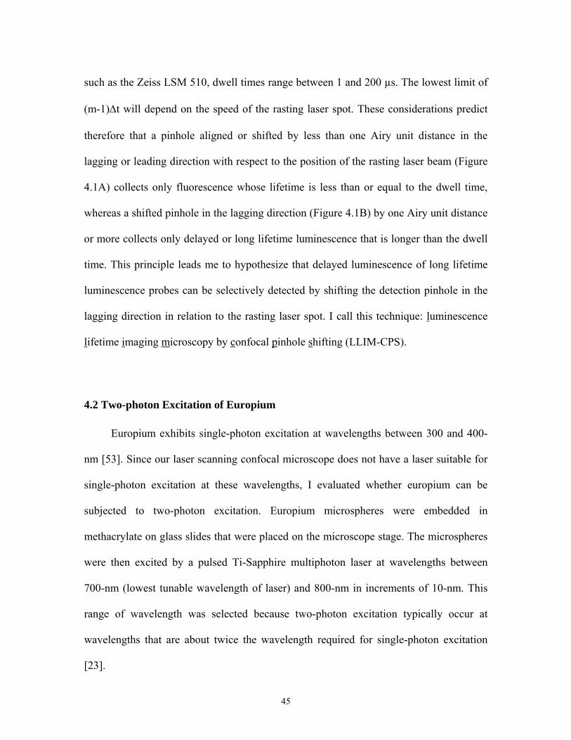
such as the Zeiss LSM 510, dwell times range between 1 and 200 µs. The lowest limit of

(m-1)Δt will depend on the speed of the rasting laser spot. These considerations predict

therefore that a pinhole aligned or shifted by less than one Airy unit distance in the

lagging or leading direction with respect to the position of the rasting laser beam (Figure

4.1A) collects only fluorescence whose lifetime is less than or equal to the dwell time,

whereas a shifted pinhole in the lagging direction (Figure 4.1B) by one Airy unit distance

or more collects only delayed or long lifetime luminescence that is longer than the dwell

time. This principle leads me to hypothesize that delayed luminescence of long lifetime

luminescence probes can be selectively detected by shifting the detection pinhole in the

lagging direction in relation to the rasting laser spot. I call this technique: luminescence

lifetime imaging microscopy by confocal pinhole shifting (LLIM-CPS).

4.2 Two-photon Excitation of Europium

Europium exhibits single-photon excitation at wavelengths between 300 and 400-

nm [53]. Since our laser scanning confocal microscope does not have a laser suitable for

single-photon excitation at these wavelengths, I evaluated whether europium can be

subjected to two-photon excitation. Europium microspheres were embedded in

methacrylate on glass slides that were placed on the microscope stage. The microspheres

were then excited by a pulsed Ti-Sapphire multiphoton laser at wavelengths between

700-nm (lowest tunable wavelength of laser) and 800-nm in increments of 10-nm. This

range of wavelength was selected because two-photon excitation typically occur at

wavelengths that are about twice the wavelength required for single-photon excitation

[23].

45

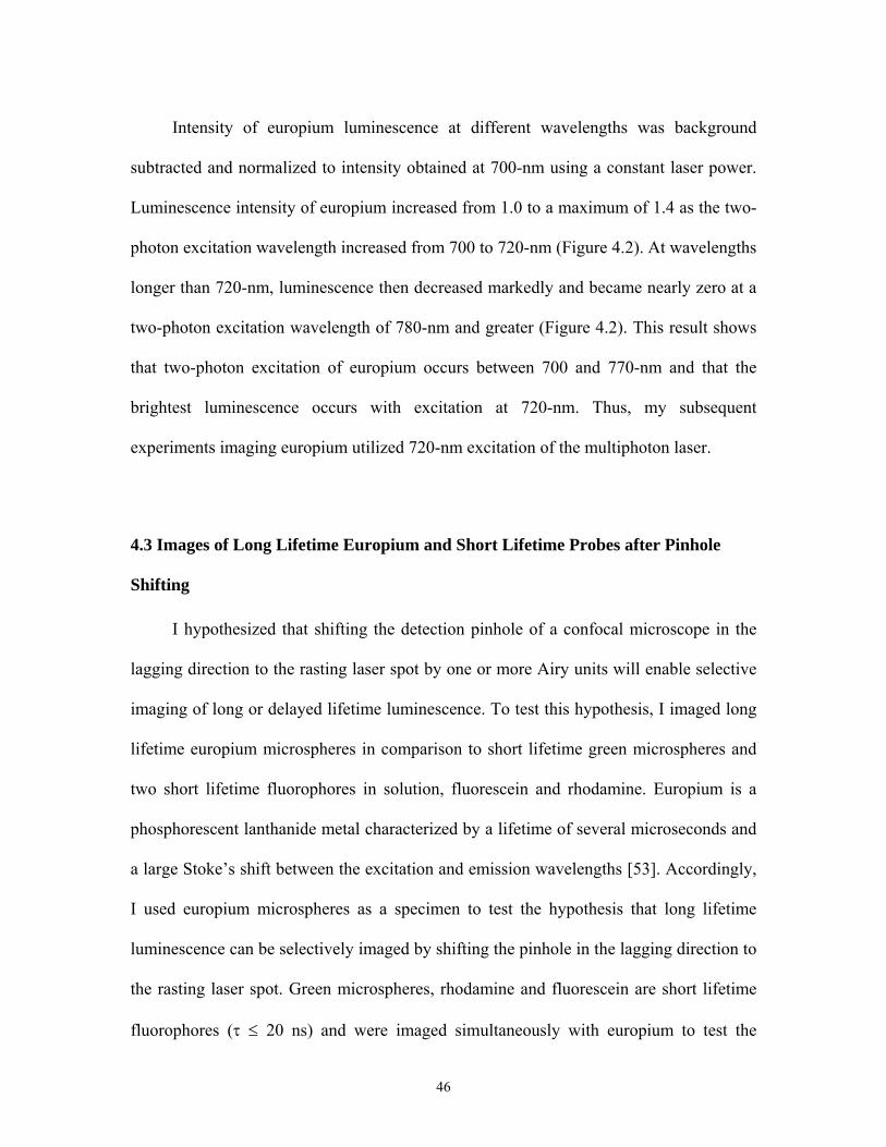
Intensity of europium luminescence at different wavelengths was background

subtracted and normalized to intensity obtained at 700-nm using a constant laser power.

Luminescence intensity of europium increased from 1.0 to a maximum of 1.4 as the two-

photon excitation wavelength increased from 700 to 720-nm (Figure 4.2). At wavelengths

longer than 720-nm, luminescence then decreased markedly and became nearly zero at a

two-photon excitation wavelength of 780-nm and greater (Figure 4.2). This result shows

that two-photon excitation of europium occurs between 700 and 770-nm and that the

brightest luminescence occurs with excitation at 720-nm. Thus, my subsequent

experiments imaging europium utilized 720-nm excitation of the multiphoton laser.

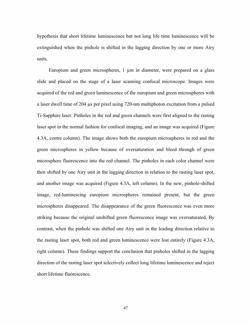
4.3 Images of Long Lifetime Europium and Short Lifetime Probes after Pinhole

Shifting

I hypothesized that shifting the detection pinhole of a confocal microscope in the

lagging direction to the rasting laser spot by one or more Airy units will enable selective

imaging of long or delayed lifetime luminescence. To test this hypothesis, I imaged long

lifetime europium microspheres in comparison to short lifetime green microspheres and

two short lifetime fluorophores in solution, fluorescein and rhodamine. Europium is a

phosphorescent lanthanide metal characterized by a lifetime of several microseconds and

a large Stoke’s shift between the excitation and emission wavelengths [53]. Accordingly,

I used europium microspheres as a specimen to test the hypothesis that long lifetime

luminescence can be selectively imaged by shifting the pinhole in the lagging direction to

the rasting laser spot. Green microspheres, rhodamine and fluorescein are short lifetime

fluorophores (τ ≤ 20 ns) and were imaged simultaneously with europium to test the

46

hypothesis that short lifetime luminescence but not long life time luminescence will be

extinguished when the pinhole is shifted in the lagging direction by one or more Airy

units.

Europium and green microspheres, 1 µm in diameter, were prepared on a glass

slide and placed on the stage of a laser scanning confocal microscope. Images were

acquired of the red and green luminescence of the europium and green microspheres with

a laser dwell time of 204 µs per pixel using 720-nm multiphoton excitation from a pulsed

Ti-Sapphire laser. Pinholes in the red and green channels were first aligned to the rasting

laser spot in the normal fashion for confocal imaging, and an image was acquired (Figure

4.3A, centre column). The image shows both the europium microspheres in red and the

green microspheres in yellow because of oversaturation and bleed through of green

microsphere fluorescence into the red channel. The pinholes in each color channel were

then shifted by one Airy unit in the lagging direction in relation to the rasting laser spot,

and another image was acquired (Figure 4.3A, left column). In the new, pinhole-shifted

image, red-luminescing europium microspheres remained present, but the green

microspheres disappeared. The disappearance of the green fluorescence was even more

striking because the original unshifted green fluorescence image was oversaturated. By

contrast, when the pinhole was shifted one Airy unit in the leading direction relative to

the rasting laser spot, both red and green luminescence were lost entirely (Figure 4.3A,

right column). These findings support the conclusion that pinholes shifted in the lagging

direction of the rasting laser spot selectively collect long lifetime luminescence and reject

short lifetime fluorescence.

47

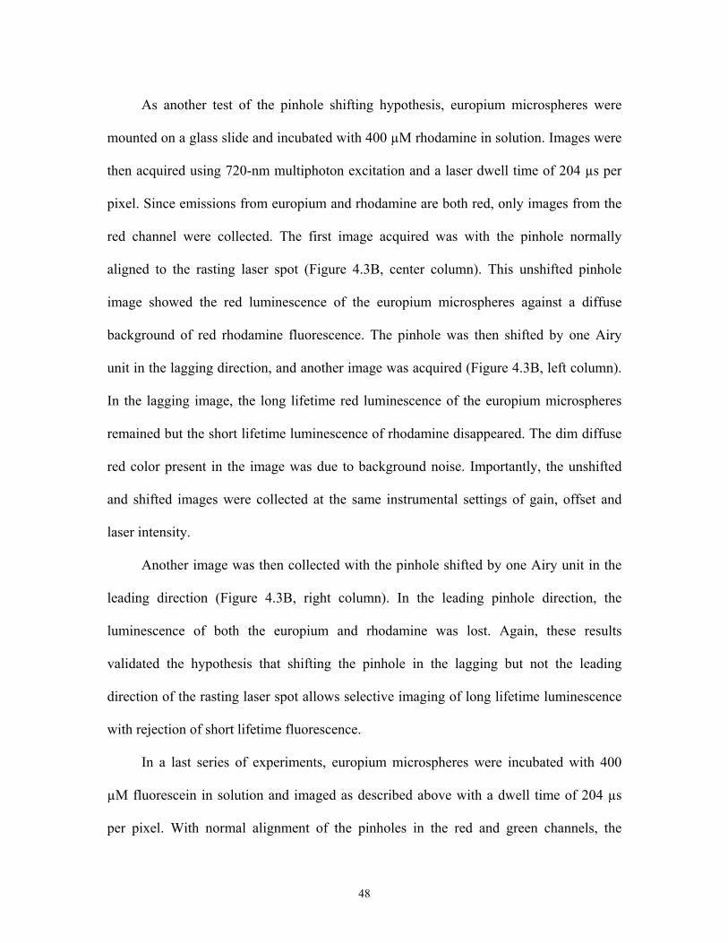
As another test of the pinhole shifting hypothesis, europium microspheres were

mounted on a glass slide and incubated with 400 µM rhodamine in solution. Images were

then acquired using 720-nm multiphoton excitation and a laser dwell time of 204 µs per

pixel. Since emissions from europium and rhodamine are both red, only images from the

red channel were collected. The first image acquired was with the pinhole normally

aligned to the rasting laser spot (Figure 4.3B, center column). This unshifted pinhole

image showed the red luminescence of the europium microspheres against a diffuse

background of red rhodamine fluorescence. The pinhole was then shifted by one Airy

unit in the lagging direction, and another image was acquired (Figure 4.3B, left column).

In the lagging image, the long lifetime red luminescence of the europium microspheres

remained but the short lifetime luminescence of rhodamine disappeared. The dim diffuse

red color present in the image was due to background noise. Importantly, the unshifted

and shifted images were collected at the same instrumental settings of gain, offset and

laser intensity.

Another image was then collected with the pinhole shifted by one Airy unit in the

leading direction (Figure 4.3B, right column). In the leading pinhole direction, the

luminescence of both the europium and rhodamine was lost. Again, these results

validated the hypothesis that shifting the pinhole in the lagging but not the leading

direction of the rasting laser spot allows selective imaging of long lifetime luminescence

with rejection of short lifetime fluorescence.

In a last series of experiments, europium microspheres were incubated with 400

µM fluorescein in solution and imaged as described above with a dwell time of 204 µs

per pixel. With normal alignment of the pinholes in the red and green channels, the

48

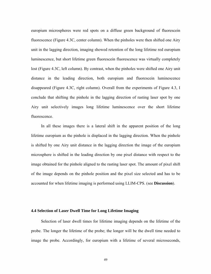
europium microspheres were red spots on a diffuse green background of fluorescein

fluorescence (Figure 4.3C, center column). When the pinholes were then shifted one Airy

unit in the lagging direction, imaging showed retention of the long lifetime red europium

luminescence, but short lifetime green fluorescein fluorescence was virtually completely

lost (Figure 4.3C, left column). By contrast, when the pinholes were shifted one Airy unit

distance in the leading direction, both europium and fluorescein luminescence

disappeared (Figure 4.3C, right column). Overall from the experiments of Figure 4.3, I

conclude that shifting the pinhole in the lagging direction of rasting laser spot by one

Airy unit selectively images long lifetime luminescence over the short lifetime

fluorescence.

In all these images there is a lateral shift in the apparent position of the long

lifetime europium as the pinhole is displaced in the lagging direction. When the pinhole

is shifted by one Airy unit distance in the lagging direction the image of the europium

microsphere is shifted in the leading direction by one pixel distance with respect to the

image obtained for the pinhole aligned to the rasting laser spot. The amount of pixel shift

of the image depends on the pinhole position and the pixel size selected and has to be

accounted for when lifetime imaging is performed using LLIM-CPS. (see Discussion).

4.4 Selection of Laser Dwell Time for Long Lifetime Imaging

Selection of laser dwell times for lifetime imaging depends on the lifetime of the

probe. The longer the lifetime of the probe; the longer will be the dwell time needed to

image the probe. Accordingly, for europium with a lifetime of several microseconds,

49

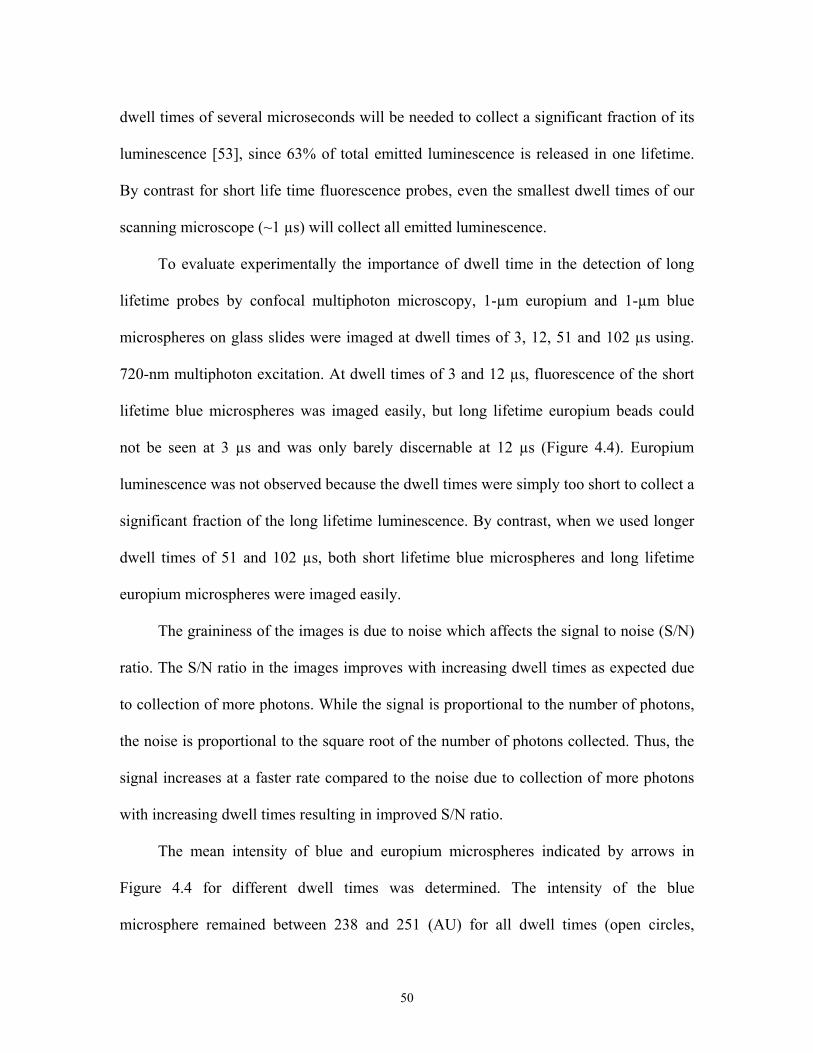
dwell times of several microseconds will be needed to collect a significant fraction of its

luminescence [53], since 63% of total emitted luminescence is released in one lifetime.

By contrast for short life time fluorescence probes, even the smallest dwell times of our

scanning microscope (~1 µs) will collect all emitted luminescence.

To evaluate experimentally the importance of dwell time in the detection of long

lifetime probes by confocal multiphoton microscopy, 1-µm europium and 1-µm blue

microspheres on glass slides were imaged at dwell times of 3, 12, 51 and 102 µs using.

720-nm multiphoton excitation. At dwell times of 3 and 12 µs, fluorescence of the short

lifetime blue microspheres was imaged easily, but long lifetime europium beads could

not be seen at 3 µs and was only barely discernable at 12 µs (Figure 4.4). Europium

luminescence was not observed because the dwell times were simply too short to collect a

significant fraction of the long lifetime luminescence. By contrast, when we used longer

dwell times of 51 and 102 µs, both short lifetime blue microspheres and long lifetime

europium microspheres were imaged easily.

The graininess of the images is due to noise which affects the signal to noise (S/N)

ratio. The S/N ratio in the images improves with increasing dwell times as expected due

to collection of more photons. While the signal is proportional to the number of photons,

the noise is proportional to the square root of the number of photons collected. Thus, the

signal increases at a faster rate compared to the noise due to collection of more photons

with increasing dwell times resulting in improved S/N ratio.

The mean intensity of blue and europium microspheres indicated by arrows in

Figure 4.4 for different dwell times was determined. The intensity of the blue

microsphere remained between 238 and 251 (AU) for all dwell times (open circles,

50

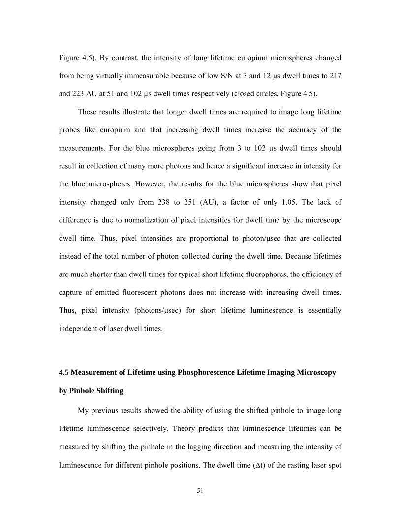
Figure 4.5). By contrast, the intensity of long lifetime europium microspheres changed

from being virtually immeasurable because of low S/N at 3 and 12 µs dwell times to 217

and 223 AU at 51 and 102 µs dwell times respectively (closed circles, Figure 4.5).

These results illustrate that longer dwell times are required to image long lifetime

probes like europium and that increasing dwell times increase the accuracy of the

measurements. For the blue microspheres going from 3 to 102 µs dwell times should

result in collection of many more photons and hence a significant increase in intensity for

the blue microspheres. However, the results for the blue microspheres show that pixel

intensity changed only from 238 to 251 (AU), a factor of only 1.05. The lack of

difference is due to normalization of pixel intensities for dwell time by the microscope

dwell time. Thus, pixel intensities are proportional to photon/μsec that are collected

instead of the total number of photon collected during the dwell time. Because lifetimes

are much shorter than dwell times for typical short lifetime fluorophores, the efficiency of

capture of emitted fluorescent photons does not increase with increasing dwell times.

Thus, pixel intensity (photons/μsec) for short lifetime luminescence is essentially

independent of laser dwell times.

4.5 Measurement of Lifetime using Phosphorescence Lifetime Imaging Microscopy

by Pinhole Shifting

My previous results showed the ability of using the shifted pinhole to image long

lifetime luminescence selectively. Theory predicts that luminescence lifetimes can be

measured by shifting the pinhole in the lagging direction and measuring the intensity of

luminescence for different pinhole positions. The dwell time (Δt) of the rasting laser spot

51

defines the duration of measurement, whereas pinhole shift defines when Δt begins and

stops in relation to luminescence decay curve. The following equations show these

relationships:

tstart = (m-1)Δt (4.2)

tstop = tstart + Δt (4.3)

where tstart and tstop are start and stop times representing a window in the luminescence

decay curve. Δt is dwell time of rasting laser spot and m is pinhole shift distance in Airy

units (m≥1). In order to measure a lifetime, at least two pinhole shifts, namely two

windows of measurement, are required.

Each pinhole shift corresponds to a time window of intensity measurement (Figure

4.6). The measured intensity at different pinhole shifts or time points can be fitted to an

exponential equation of the form I = e-t/τ where I is the intensity measured for time

window t. From this fitting, the lifetime (τ) is estimated. For two measurements made at

two different pinhole shifts, lifetime can be also calculated by the following equation:

[31]

τ = − Δt/ln(I1/Io) (4.4)

where τ is lifetime of the fluorophore or phosphor, and Io and I1 are intensities measured

at the two pinhole shifts.

The validity and utility of these equations was evaluated using 1-μm diameter

europium microspheres, which have a lifetime of hundreds of microseconds [53].

Europium microspheres on glass slides were imaged using 720-nm multiphoton

52

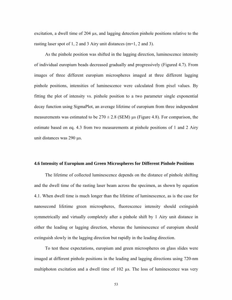
excitation, a dwell time of 204 µs, and lagging detection pinhole positions relative to the

rasting laser spot of 1, 2 and 3 Airy unit distances (m=1, 2 and 3).

As the pinhole position was shifted in the lagging direction, luminescence intensity

of individual europium beads decreased gradually and progressively (Figured 4.7). From

images of three different europium microspheres imaged at three different lagging

pinhole positions, intensities of luminescence were calculated from pixel values. By

fitting the plot of intensity vs. pinhole position to a two parameter single exponential

decay function using SigmaPlot, an average lifetime of europium from three independent

measurements was estimated to be 270 ± 2.8 (SEM) µs (Figure 4.8). For comparison, the

estimate based on eq. 4.3 from two measurements at pinhole positions of 1 and 2 Airy

unit distances was 290 µs.

4.6 Intensity of Europium and Green Microspheres for Different Pinhole Positions

The lifetime of collected luminescence depends on the distance of pinhole shifting

and the dwell time of the rasting laser beam across the specimen, as shown by equation

4.1. When dwell time is much longer than the lifetime of luminescence, as is the case for

nanosecond lifetime green microspheres, fluorescence intensity should extinguish

symmetrically and virtually completely after a pinhole shift by 1 Airy unit distance in

either the leading or lagging direction, whereas the luminescence of europium should

extinguish slowly in the lagging direction but rapidly in the leading direction.

To test these expectations, europium and green microspheres on glass slides were

imaged at different pinhole positions in the leading and lagging directions using 720-nm

multiphoton excitation and a dwell time of 102 µs. The loss of luminescence was very

53

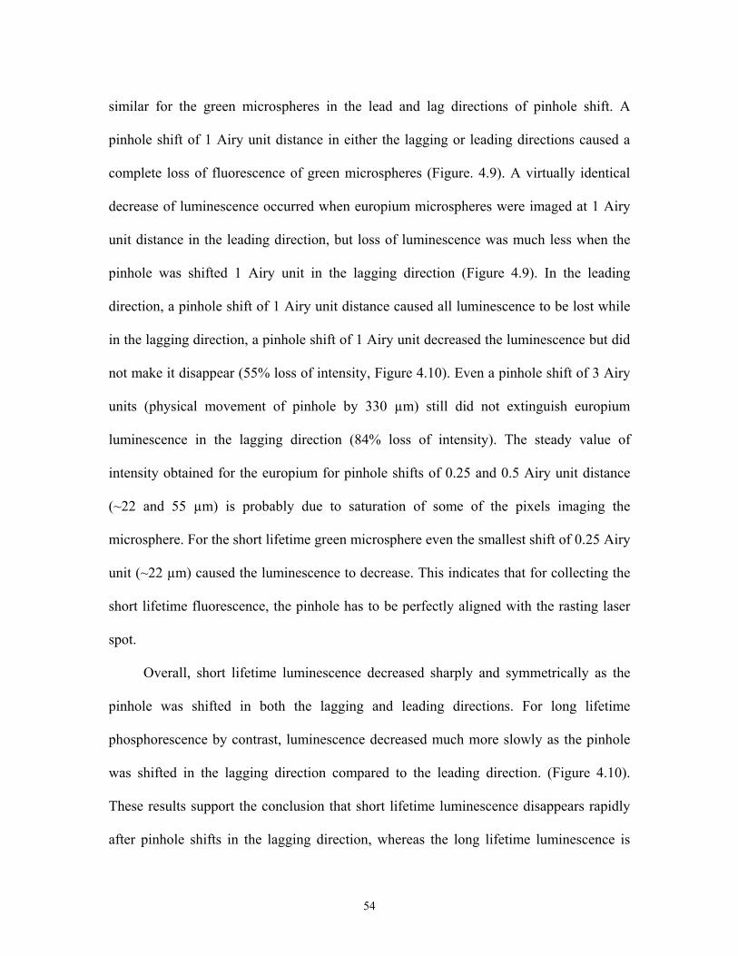
similar for the green microspheres in the lead and lag directions of pinhole shift. A

pinhole shift of 1 Airy unit distance in either the lagging or leading directions caused a

complete loss of fluorescence of green microspheres (Figure. 4.9). A virtually identical

decrease of luminescence occurred when europium microspheres were imaged at 1 Airy

unit distance in the leading direction, but loss of luminescence was much less when the

pinhole was shifted 1 Airy unit in the lagging direction (Figure 4.9). In the leading

direction, a pinhole shift of 1 Airy unit distance caused all luminescence to be lost while

in the lagging direction, a pinhole shift of 1 Airy unit decreased the luminescence but did

not make it disappear (55% loss of intensity, Figure 4.10). Even a pinhole shift of 3 Airy

units (physical movement of pinhole by 330 µm) still did not extinguish europium

luminescence in the lagging direction (84% loss of intensity). The steady value of

intensity obtained for the europium for pinhole shifts of 0.25 and 0.5 Airy unit distance

(~22 and 55 µm) is probably due to saturation of some of the pixels imaging the

microsphere. For the short lifetime green microsphere even the smallest shift of 0.25 Airy

unit (~22 µm) caused the luminescence to decrease. This indicates that for collecting the

short lifetime fluorescence, the pinhole has to be perfectly aligned with the rasting laser

spot.

Overall, short lifetime luminescence decreased sharply and symmetrically as the

pinhole was shifted in both the lagging and leading directions. For long lifetime

phosphorescence by contrast, luminescence decreased much more slowly as the pinhole

was shifted in the lagging direction compared to the leading direction. (Figure 4.10).

These results support the conclusion that short lifetime luminescence disappears rapidly

after pinhole shifts in the lagging direction, whereas the long lifetime luminescence is

54

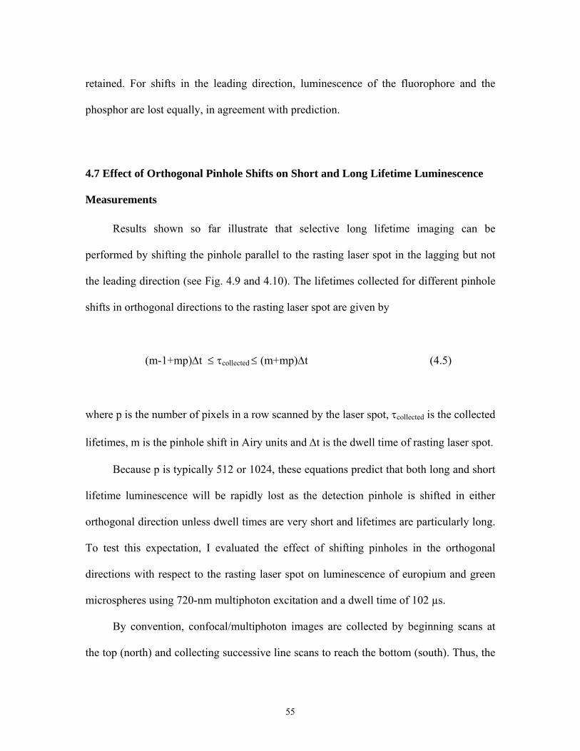
retained. For shifts in the leading direction, luminescence of the fluorophore and the

phosphor are lost equally, in agreement with prediction.

4.7 Effect of Orthogonal Pinhole Shifts on Short and Long Lifetime Luminescence

Measurements

Results shown so far illustrate that selective long lifetime imaging can be

performed by shifting the pinhole parallel to the rasting laser spot in the lagging but not

the leading direction (see Fig. 4.9 and 4.10). The lifetimes collected for different pinhole

shifts in orthogonal directions to the rasting laser spot are given by

(m-1+mp)Δt ≤ τcollected ≤ (m+mp)Δt (4.5)

where p is the number of pixels in a row scanned by the laser spot, τcollected is the collected

lifetimes, m is the pinhole shift in Airy units and Δt is the dwell time of rasting laser spot.

Because p is typically 512 or 1024, these equations predict that both long and short

lifetime luminescence will be rapidly lost as the detection pinhole is shifted in either

orthogonal direction unless dwell times are very short and lifetimes are particularly long.

To test this expectation, I evaluated the effect of shifting pinholes in the orthogonal

directions with respect to the rasting laser spot on luminescence of europium and green

microspheres using 720-nm multiphoton excitation and a dwell time of 102 µs.

By convention, confocal/multiphoton images are collected by beginning scans at

the top (north) and collecting successive line scans to reach the bottom (south). Thus, the

55

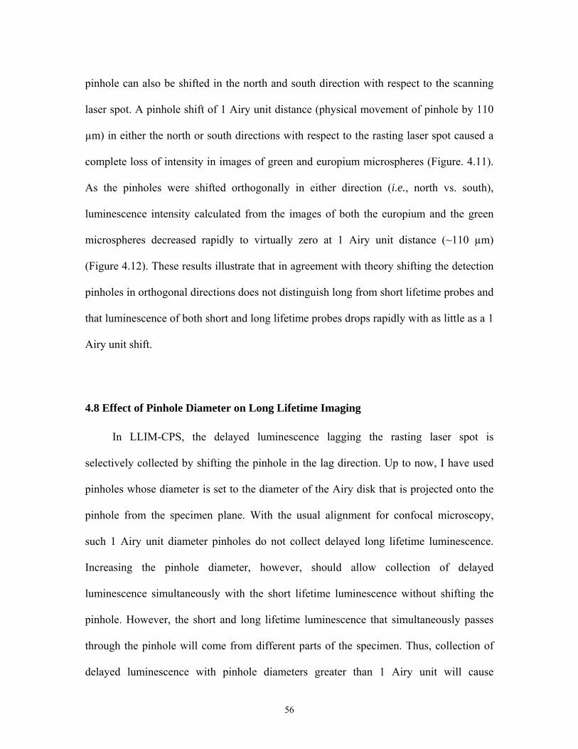
pinhole can also be shifted in the north and south direction with respect to the scanning

laser spot. A pinhole shift of 1 Airy unit distance (physical movement of pinhole by 110

µm) in either the north or south directions with respect to the rasting laser spot caused a

complete loss of intensity in images of green and europium microspheres (Figure. 4.11).

As the pinholes were shifted orthogonally in either direction (i.e., north vs. south),

luminescence intensity calculated from the images of both the europium and the green

microspheres decreased rapidly to virtually zero at 1 Airy unit distance (~110 µm)

(Figure 4.12). These results illustrate that in agreement with theory shifting the detection

pinholes in orthogonal directions does not distinguish long from short lifetime probes and

that luminescence of both short and long lifetime probes drops rapidly with as little as a 1

Airy unit shift.

4.8 Effect of Pinhole Diameter on Long Lifetime Imaging

In LLIM-CPS, the delayed luminescence lagging the rasting laser spot is

selectively collected by shifting the pinhole in the lag direction. Up to now, I have used

pinholes whose diameter is set to the diameter of the Airy disk that is projected onto the

pinhole from the specimen plane. With the usual alignment for confocal microscopy,

such 1 Airy unit diameter pinholes do not collect delayed long lifetime luminescence.

Increasing the pinhole diameter, however, should allow collection of delayed

luminescence simultaneously with the short lifetime luminescence without shifting the

pinhole. However, the short and long lifetime luminescence that simultaneously passes

through the pinhole will come from different parts of the specimen. Thus, collection of

delayed luminescence with pinhole diameters greater than 1 Airy unit will cause

56

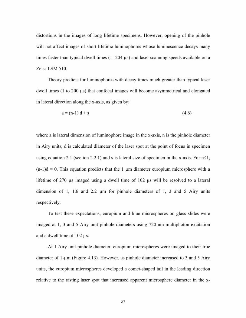
distortions in the images of long lifetime specimens. However, opening of the pinhole

will not affect images of short lifetime luminophores whose luminescence decays many

times faster than typical dwell times (1- 204 µs) and laser scanning speeds available on a

Zeiss LSM 510.

Theory predicts for luminophores with decay times much greater than typical laser

dwell times (1 to 200 µs) that confocal images will become asymmetrical and elongated

in lateral direction along the x-axis, as given by:

a = (n-1) d + s (4.6)

where a is lateral dimension of luminophore image in the x-axis, n is the pinhole diameter

in Airy units, d is calculated diameter of the laser spot at the point of focus in specimen

using equation 2.1 (section 2.2.1) and s is lateral size of specimen in the x-axis. For n≤1,

(n-1)d = 0. This equation predicts that the 1 µm diameter europium microsphere with a

lifetime of 270 µs imaged using a dwell time of 102 µs will be resolved to a lateral

dimension of 1, 1.6 and 2.2 µm for pinhole diameters of 1, 3 and 5 Airy units

respectively.

To test these expectations, europium and blue microspheres on glass slides were

imaged at 1, 3 and 5 Airy unit pinhole diameters using 720-nm multiphoton excitation

and a dwell time of 102 µs.

At 1 Airy unit pinhole diameter, europium microspheres were imaged to their true

diameter of 1-µm (Figure 4.13). However, as pinhole diameter increased to 3 and 5 Airy

units, the europium microspheres developed a comet-shaped tail in the leading direction

relative to the rasting laser spot that increased apparent microsphere diameter in the x-

57

direction to 1.5 and 2.1 µm, respectively, close to the predicted values. By contrast, the

europium microspheres were resolved to their true diameter of 1-µm in the y-direction at

all pinhole diameters.

By contrast, the diameter of short lifetime blue microspheres in confocal images

remained 1-µm at all pinhole diameters. The blue microspheres were saturated, which

caused blooming of the images and should have exaggerated any distortion, but the true

shape of the blue microspheres was maintained at all pinhole diameters. These results

showed long lifetime objects will not be imaged at their true dimensions at detection

pinhole diameters greater than 1 Airy unit. This distortion is because larger pinholes also

collect long lifetime luminescence emitted from positions lagging behind the scanning

laser spot. This long lifetime luminescence is then recorded in pixels at positions in the

leading direction to the actual source causing distortions in the image. Ultimately the

presence of these distortions and their magnitude will depend on the diameter of pinhole,

dwell time of rasting laser spot, and lifetime of the specimen. Predictions of the expected

image shape and size may enable software adjustment of long lifetime images acquired

with larger pinhole diameters.

4.9 Effect of Pinhole Diameter on Pinhole Shifting

To collect short lifetime luminescence, the pinhole in the image plane has to be

aligned in register with the crossover point of the rasting laser beam in the specimen

plane. Hence, the pinhole and the laser spot are “confocal” with one another. Any shift

from the aligned position decreases the registration and thus the amount of short lifetime

luminescence collected through the pinhole. When the pinhole is displaced laterally by

58

the diameter of the diffraction-limited laser spot (1 Airy unit), virtually all overlap is lost,

and short lifetime luminescence decreases sharply. However, when the pinhole is

displaced in the lagging direction, long lifetime luminescence can still be collected. This

principle forms the basis for selectively imaging of long lifetime luminescence (Figure

4.1, 4.9 and 4.10).

Theory predicts that the pinhole shift distance required to remove this overlap and

selectively collect the decaying long lifetime luminescence should increase with

increasing pinhole diameters. This distance of pinhole shift required to remove any

overlap in the lag direction and selectively collect the long lifetime luminescence s given

by:

m = (n + 1)/2 (4.7)

where m is pinhole shift distance in Airy units and n is pinhole diameter in Airy units.

This equation predicts that pinhole shifts of 1, 2 and 3 Airy units distance in the lag

direction are required to remove any overlap between the laser spot and pinhole and

selectively collect the long lifetime luminescence for pinhole diameters of 1, 3 and 5 Airy

units, respectively.

To test this expectation, images of europium microspheres on glass slides were

acquired for different leading and lagging pinhole positions at 1, 3 and 5 Airy unit

pinhole diameters using 720-nm multiphoton excitation and a dwell time of 102 µs.

For a pinhole diameter of 1 Airy unit even a pinhole shift of 1 Airy unit (physical

shift of 110 µm) in the lagging direction caused the luminescence to decrease by 5% of

the luminescence intensity for the aligned pinhole position (Figure 4.14, open circles).

59

Further increases in distance consistently decreased the intensity with the intensity

decreasing by 85% of the intensity for the pinhole shift at 4 Airy units.

For a pinhole diameter of 3 Airy unit the luminescence intensity remained constant

till a pinhole shift of 1 Airy unit distance. A pinhole shift of 2 Airy units (physical shift of

220 µm) caused the luminescence to decrease by 15% (open triangles). The constant

value of intensity in the lagging direction for pinhole shifts of up to 1 Airy unit distance

represents the overlap of the pinhole with the rasting laser spot. Increases in the pinhole

shift distance beyond 2 Airy units distance consistently decreased the intensity.

For a pinhole diameter of 5 Airy unit, intensity of europium luminescence collected

remained constant until a pinhole shift of 1 and 2 Airy units distance while a pinhole shift

of 3 Airy units (physical shift of 330 µm) caused the luminescence to decrease by 25%

(open squares). Again the constant value of intensity in the lagging direction for pinhole

shifts of up to 2 Airy units distance represents the overlap of the pinhole with the rasting

laser spot. Increases in the pinhole shift distance beyond 3 Airy units distance

consistently decreased the intensity. These results support the prediction of increasing

pinhole diameters requiring increasing pinhole shifts to remove overlap of pinhole with

laser cross over point and selectively image long lifetime luminescence.

Further a pinhole shift of 3 Airy units distance (~330 µm physical movement)

caused the luminescence of europium to decrease by 70, 50 and 25% for 1, 3 and 5 Airy

unit pinhole diameters respectively. A pinhole shift of 4 Airy units distance (~440 µm

physical movement) caused luminescence of europium to decrease by 85, 60 and 50% for

1, 3 and 5 Airy unit pinhole diameters respectively. These results indicate that same

60

amount of pinhole shift distance for different pinhole diameters will collect different

times of the luminescence decay.

Our results in section 4.6 (Figure 4.10 and 4.11) for a one Airy unit pinhole

diameter showed that in the leading direction even the long lifetime europium

luminescence decreases to zero for a pinhole shift of one Airy units distance. Our results

here support this evidence that in the leading direction, a pinhole shift of 1 Airy unit

caused luminescence to decrease below detectable levels for the 1 Airy unit diameter

pinhole (Figure 4.14, open circles). However, for pinhole diameters of 3 and 5 Airy unit,

(Figure 4.14, open triangles and squares) luminescence persisted beyond a pinhole shift

of 1 Airy unit distance in the leading direction and decreased below detectable levels only

at a distance of 3 and 4 Airy units distances in the leading direction respectively. Thus,

for pinhole diameters greater than 1 Airy unit, long lifetime luminescence was retained

beyond 1 Airy unit distance for pinhole shifts even in the leading direction.

4.10 Testing Oxyrase for Oxygen Removal

Oxyrase is a commercial oxygen-consuming enzyme mixture of bacterial origin.

The oxygen-reducing activity of oxyrase starts when oxyrase comes in contact with

oxygen and a hydrogen donor, such as lactate, succinate, formate and alpha-glycerol

phosphate, which are included in the mixture (Oxyrase Inc., Mansfield, Ohio). In order to

test the ability of oxyrase to remove oxygen, oxygen consumption by 1, 2 and 4%

oxyrase in KRH was determined with a Clark oxygen electrode.

After addition of 1, 2 and 4% oxyrase to the closed oxygen electrode chamber,

oxygen concentration decreased from air-saturation (20% oxygen or 150 Torr pressure)

61

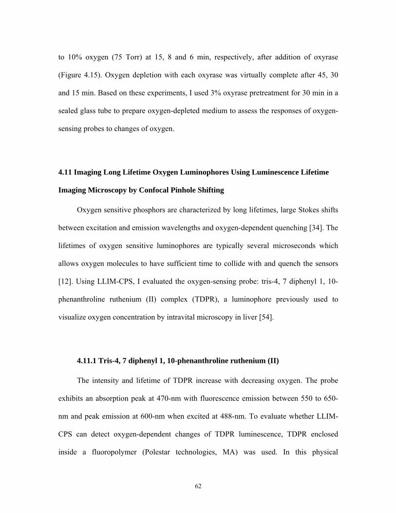
to 10% oxygen (75 Torr) at 15, 8 and 6 min, respectively, after addition of oxyrase

(Figure 4.15). Oxygen depletion with each oxyrase was virtually complete after 45, 30

and 15 min. Based on these experiments, I used 3% oxyrase pretreatment for 30 min in a

sealed glass tube to prepare oxygen-depleted medium to assess the responses of oxygen-

sensing probes to changes of oxygen.

4.11 Imaging Long Lifetime Oxygen Luminophores Using Luminescence Lifetime

Imaging Microscopy by Confocal Pinhole Shifting

Oxygen sensitive phosphors are characterized by long lifetimes, large Stokes shifts

between excitation and emission wavelengths and oxygen-dependent quenching [34]. The

lifetimes of oxygen sensitive luminophores are typically several microseconds which

allows oxygen molecules to have sufficient time to collide with and quench the sensors

[12]. Using LLIM-CPS, I evaluated the oxygen-sensing probe: tris-4, 7 diphenyl 1, 10-

phenanthroline ruthenium (II) complex (TDPR), a luminophore previously used to

visualize oxygen concentration by intravital microscopy in liver [54].

4.11.1 Tris-4, 7 diphenyl 1, 10-phenanthroline ruthenium (II)

The intensity and lifetime of TDPR increase with decreasing oxygen. The probe

exhibits an absorption peak at 470-nm with fluorescence emission between 550 to 650-

nm and peak emission at 600-nm when excited at 488-nm. To evaluate whether LLIM-

CPS can detect oxygen-dependent changes of TDPR luminescence, TDPR enclosed

inside a fluoropolymer (Polestar technologies, MA) was used. In this physical

62

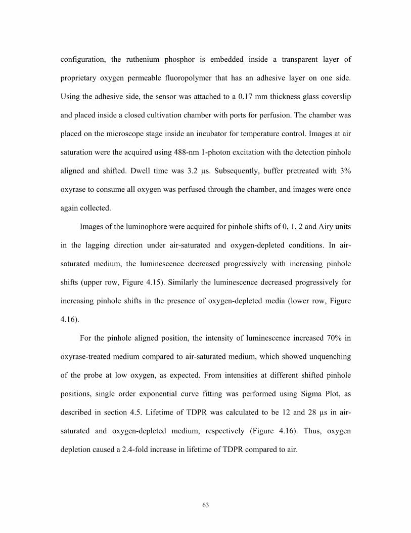
configuration, the ruthenium phosphor is embedded inside a transparent layer of

proprietary oxygen permeable fluoropolymer that has an adhesive layer on one side.

Using the adhesive side, the sensor was attached to a 0.17 mm thickness glass coverslip

and placed inside a closed cultivation chamber with ports for perfusion. The chamber was

placed on the microscope stage inside an incubator for temperature control. Images at air

saturation were the acquired using 488-nm 1-photon excitation with the detection pinhole

aligned and shifted. Dwell time was 3.2 µs. Subsequently, buffer pretreated with 3%

oxyrase to consume all oxygen was perfused through the chamber, and images were once

again collected.

Images of the luminophore were acquired for pinhole shifts of 0, 1, 2 and Airy units

in the lagging direction under air-saturated and oxygen-depleted conditions. In air-

saturated medium, the luminescence decreased progressively with increasing pinhole

shifts (upper row, Figure 4.15). Similarly the luminescence decreased progressively for

increasing pinhole shifts in the presence of oxygen-depleted media (lower row, Figure

4.16).

For the pinhole aligned position, the intensity of luminescence increased 70% in

oxyrase-treated medium compared to air-saturated medium, which showed unquenching

of the probe at low oxygen, as expected. From intensities at different shifted pinhole

positions, single order exponential curve fitting was performed using Sigma Plot, as

described in section 4.5. Lifetime of TDPR was calculated to be 12 and 28 µs in air-

saturated and oxygen-depleted medium, respectively (Figure 4.16). Thus, oxygen

depletion caused a 2.4-fold increase in lifetime of TDPR compared to air.

63

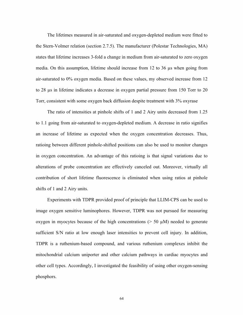
The lifetimes measured in air-saturated and oxygen-depleted medium were fitted to

the Stern-Volmer relation (section 2.7.5). The manufacturer (Polestar Technologies, MA)

states that lifetime increases 3-fold a change in medium from air-saturated to zero oxygen

media. On this assumption, lifetime should increase from 12 to 36 µs when going from

air-saturated to 0% oxygen media. Based on these values, my observed increase from 12

to 28 µs in lifetime indicates a decrease in oxygen partial pressure from 150 Torr to 20

Torr, consistent with some oxygen back diffusion despite treatment with 3% oxyrase

The ratio of intensities at pinhole shifts of 1 and 2 Airy units decreased from 1.25

to 1.1 going from air-saturated to oxygen-depleted medium. A decrease in ratio signifies

an increase of lifetime as expected when the oxygen concentration decreases. Thus,

ratioing between different pinhole-shifted positions can also be used to monitor changes

in oxygen concentration. An advantage of this ratioing is that signal variations due to

alterations of probe concentration are effectively canceled out. Moreover, virtually all

contribution of short lifetime fluorescence is eliminated when using ratios at pinhole

shifts of 1 and 2 Airy units.

Experiments with TDPR provided proof of principle that LLIM-CPS can be used to

image oxygen sensitive luminophores. However, TDPR was not pursued for measuring

oxygen in myocytes because of the high concentrations (> 50 µM) needed to generate

sufficient S/N ratio at low enough laser intensities to prevent cell injury. In addition,

TDPR is a ruthenium-based compound, and various ruthenium complexes inhibit the

mitochondrial calcium uniporter and other calcium pathways in cardiac myocytes and

other cell types. Accordingly, I investigated the feasibility of using other oxygen-sensing

phosphors.

64

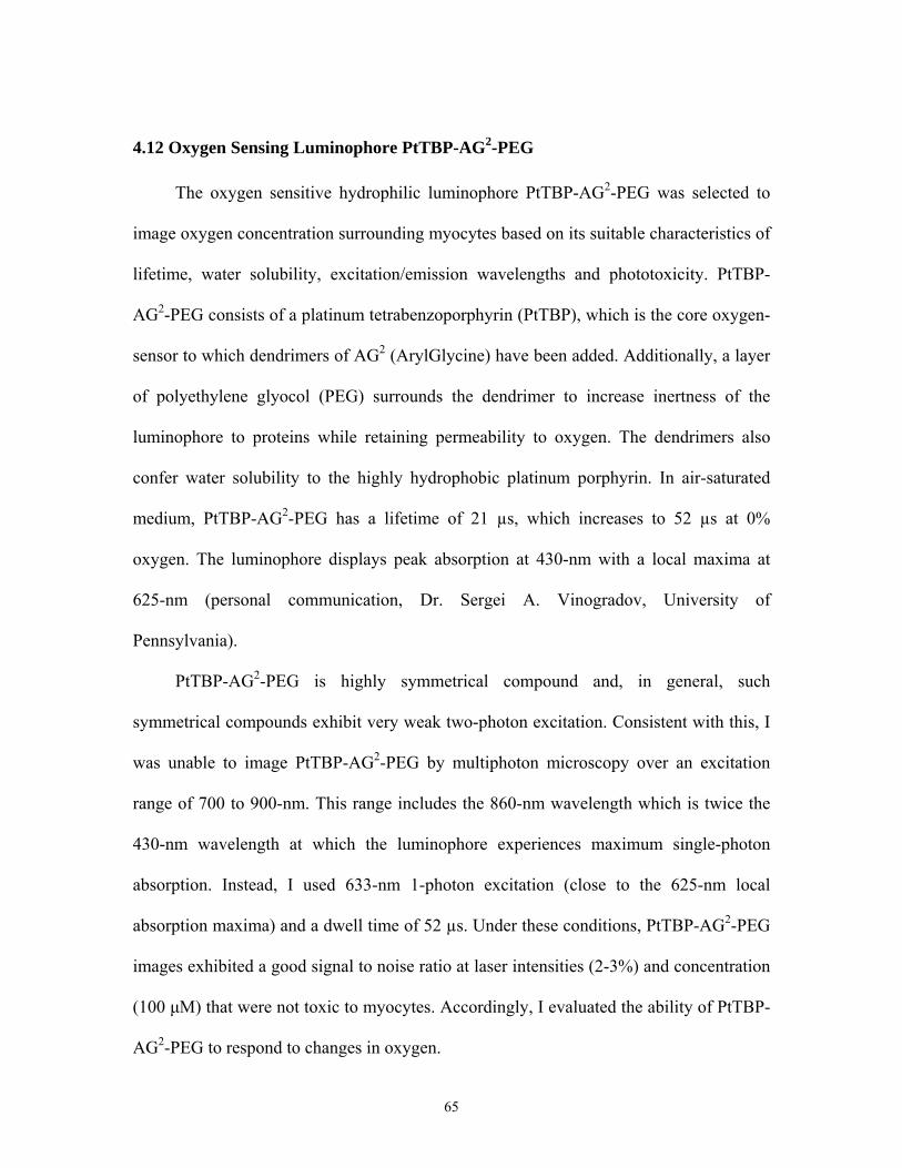
4.12 Oxygen Sensing Luminophore PtTBP-AG2-PEG

The oxygen sensitive hydrophilic luminophore PtTBP-AG2-PEG was selected to

image oxygen concentration surrounding myocytes based on its suitable characteristics of

lifetime, water solubility, excitation/emission wavelengths and phototoxicity. PtTBP-

AG2-PEG consists of a platinum tetrabenzoporphyrin (PtTBP), which is the core oxygen-

sensor to which dendrimers of AG2 (ArylGlycine) have been added. Additionally, a layer

of polyethylene glyocol (PEG) surrounds the dendrimer to increase inertness of the

luminophore to proteins while retaining permeability to oxygen. The dendrimers also

confer water solubility to the highly hydrophobic platinum porphyrin. In air-saturated

medium, PtTBP-AG2-PEG has a lifetime of 21 µs, which increases to 52 µs at 0%

oxygen. The luminophore displays peak absorption at 430-nm with a local maxima at

625-nm (personal communication, Dr. Sergei A. Vinogradov, University of

Pennsylvania).

PtTBP-AG2-PEG is highly symmetrical compound and, in general, such

symmetrical compounds exhibit very weak two-photon excitation. Consistent with this, I

was unable to image PtTBP-AG2-PEG by multiphoton microscopy over an excitation

range of 700 to 900-nm. This range includes the 860-nm wavelength which is twice the

430-nm wavelength at which the luminophore experiences maximum single-photon

absorption. Instead, I used 633-nm 1-photon excitation (close to the 625-nm local

absorption maxima) and a dwell time of 52 µs. Under these conditions, PtTBP-AG2-PEG

images exhibited a good signal to noise ratio at laser intensities (2-3%) and concentration

(100 μM) that were not toxic to myocytes. Accordingly, I evaluated the ability of PtTBP-

AG2-PEG to respond to changes in oxygen.

65

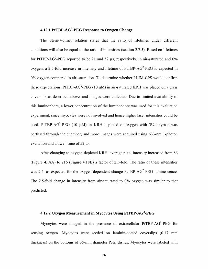
4.12.1 PtTBP-AG2-PEG Response to Oxygen Change

The Stern-Volmer relation states that the ratio of lifetimes under different

conditions will also be equal to the ratio of intensities (section 2.7.5). Based on lifetimes

for PtTBP-AG2-PEG reported to be 21 and 52 µs, respectively, in air-saturated and 0%

oxygen, a 2.5-fold increase in intensity and lifetime of PtTBP-AG2-PEG is expected in

0% oxygen compared to air-saturation. To determine whether LLIM-CPS would confirm

these expectations, PtTBP-AG2-PEG (10 μM) in air-saturated KRH was placed on a glass

coverslip, as described above, and images were collected. Due to limited availability of

this luminophore, a lower concentration of the luminophore was used for this evaluation

experiment, since myocytes were not involved and hence higher laser intensities could be

used. PtTBP-AG2-PEG (10 µM) in KRH depleted of oxygen with 3% oxyrase was

perfused through the chamber, and more images were acquired using 633-nm 1-photon

excitation and a dwell time of 52 µs.

After changing to oxygen-depleted KRH, average pixel intensity increased from 86

(Figure 4.18A) to 216 (Figure 4.18B) a factor of 2.5-fold. The ratio of these intensities

was 2.5, as expected for the oxygen-dependent change PtTBP-AG2-PEG luminescence.

The 2.5-fold change in intensity from air-saturated to 0% oxygen was similar to that

predicted.

4.12.2 Oxygen Measurement in Myocytes Using PtTBP-AG2-PEG

Myocytes were imaged in the presence of extracellular PtTBP-AG2-PEG for

sensing oxygen. Myocytes were seeded on laminin-coated coverslips (0.17 mm

thickness) on the bottoms of 35-mm diameter Petri dishes. Myocytes were labeled with

66

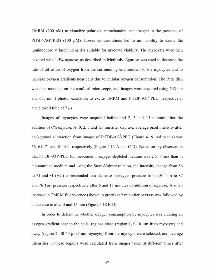
TMRM (200 nM) to visualize polarized mitochondria and imaged in the presence of

PtTBP-AG2-PEG (100 µM). Lower concentrations led to an inability to excite the

luminophore at laser intensities suitable for myocyte viability. The myocytes were then

covered with 1.5% agarose, as described in Methods. Agarose was used to decrease the

rate of diffusion of oxygen from the surrounding environment to the myocytes and to

increase oxygen gradients near cells due to cellular oxygen consumption. The Petri dish

was then mounted on the confocal microscope, and images were acquired using 543-nm

and 633-nm 1-photon excitation to excite TMRM and PtTBP-AG2-PEG, respectively,

and a dwell time of 7 µs.

Images of myocytes were acquired before and 2, 5 and 15 minutes after the

addition of 6% oxyrase. At 0, 2, 5 and 15 min after oxyrase, average pixel intensity after

background subtraction from images of PtTBP-AG2-PEG (Figure 4.19, red panels) was

56, 61, 71 and 81 AU, respectively (Figure 4.13 A and C-D). Based on my observation

that PtTBP-AG2-PEG luminescence in oxygen-depleted medium was 2.51 times than in

air-saturated medium and using the Stern-Volmer relation, the intensity change from 56

to 71 and 81 (AU) corresponded to a decrease in oxygen pressure from 150 Torr to 87

and 76 Torr pressure respectively after 5 and 15 minutes of addition of oxyrase. A small

increase in TMRM fluorescence (shown in green) at 2 min after oxyrase was followed by

a decrease in after 5 and 15 min (Figure 4.18 B-D).

In order to determine whether oxygen consumption by myocytes was creating an

oxygen gradient next to the cells, regions close (region 1, 0-10 µm from myocyte) and

away (region 2, 40-50 µm from myocyte) from the myocyte were selected, and average

intensities in these regions were calculated from images taken at different times after

67

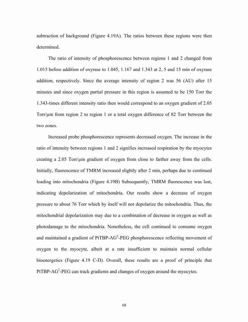
subtraction of background (Figure 4.19A). The ratios between these regions were then

determined.

The ratio of intensity of phosphorescence between regions 1 and 2 changed from

1.015 before addition of oxyrase to 1.045, 1.167 and 1.343 at 2, 5 and 15 min of oxyrase

addition, respectively. Since the average intensity of region 2 was 56 (AU) after 15

minutes and since oxygen partial pressure in this region is assumed to be 150 Torr the

1.343-times different intensity ratio then would correspond to an oxygen gradient of 2.05

Torr/µm from region 2 to region 1 or a total oxygen difference of 82 Torr between the

two zones.

Increased probe phosphorescence represents decreased oxygen. The increase in the

ratio of intensity between regions 1 and 2 signifies increased respiration by the myocytes

creating a 2.05 Torr/µm gradient of oxygen from close to farther away from the cells.

Initially, fluorescence of TMRM increased slightly after 2 min, perhaps due to continued

loading into mitochondria (Figure 4.19B) Subsequently, TMRM fluorescence was lost,

indicating depolarization of mitochondria. Our results show a decrease of oxygen

pressure to about 76 Torr which by itself will not depolarize the mitochondria. Thus, the

mitochondrial depolarization may due to a combination of decrease in oxygen as well as

photodamage to the mitochondria. Nonetheless, the cell continued to consume oxygen

and maintained a gradient of PtTBP-AG2-PEG phosphorescence reflecting movement of

oxygen to the myocyte, albeit at a rate insufficient to maintain normal cellular

bioenergetics (Figure 4.19 C-D). Overall, these results are a proof of principle that

PtTBP-AG2-PEG can track gradients and changes of oxygen around the myocytes.

68

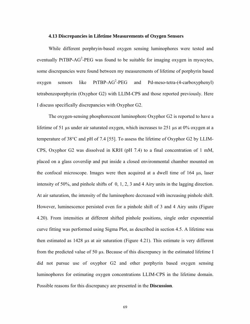
4.13 Discrepancies in Lifetime Measurements of Oxygen Sensors

While different porphryin-based oxygen sensing luminophores were tested and

eventually PtTBP-AG2-PEG was found to be suitable for imaging oxygen in myocytes,

some discrepancies were found between my measurements of lifetime of porphyrin based

oxygen sensors like PtTBP-AG2-PEG and Pd-meso-tetra-(4-carboxyphenyl)

tetrabenzoporphyrin (Oxyphor G2) with LLIM-CPS and those reported previously. Here

I discuss specifically discrepancies with Oxyphor G2.

The oxygen-sensing phosphorescent luminophore Oxyphor G2 is reported to have a

lifetime of 51 µs under air saturated oxygen, which increases to 251 µs at 0% oxygen at a

temperature of 38°C and pH of 7.4 [55]. To assess the lifetime of Oxyphor G2 by LLIM-

CPS, Oxyphor G2 was dissolved in KRH (pH 7.4) to a final concentration of 1 mM,

placed on a glass coverslip and put inside a closed environmental chamber mounted on

the confocal microscope. Images were then acquired at a dwell time of 164 µs, laser

intensity of 50%, and pinhole shifts of 0, 1, 2, 3 and 4 Airy units in the lagging direction.

At air saturation, the intensity of the luminophore decreased with increasing pinhole shift.

However, luminescence persisted even for a pinhole shift of 3 and 4 Airy units (Figure

4.20). From intensities at different shifted pinhole positions, single order exponential

curve fitting was performed using Sigma Plot, as described in section 4.5. A lifetime was

then estimated as 1428 µs at air saturation (Figure 4.21). This estimate is very different

from the predicted value of 50 µs. Because of this discrepancy in the estimated lifetime I

did not pursue use of oxyphor G2 and other porphyrin based oxygen sensing

luminophores for estimating oxygen concentrations LLIM-CPS in the lifetime domain.

Possible reasons for this discrepancy are presented in the Discussion.

69

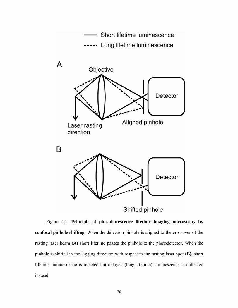
Figure 4.1. Principle of phosphorescence lifetime imaging microscopy by

confocal pinhole shifting. When the detection pinhole is aligned to the crossover of the

rasting laser beam (A) short lifetime passes the pinhole to the photodetector. When the

pinhole is shifted in the lagging direction with respect to the rasting laser spot (B), short

lifetime luminescence is rejected but delayed (long lifetime) luminescence is collected

instead.

70

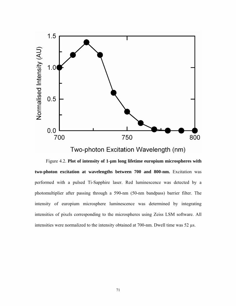
Figure 4.2. Plot of intensity of 1-µm long lifetime europium microspheres with

two-photon excitation at wavelengths between 700 and 800-nm. Excitation was

performed with a pulsed Ti-Sapphire laser. Red luminescence was detected by a

photomultiplier after passing through a 590-nm (50-nm bandpass) barrier filter. The

intensity of europium microsphere luminescence was determined by integrating

intensities of pixels corresponding to the microspheres using Zeiss LSM software. All

intensities were normalized to the intensity obtained at 700-nm. Dwell time was 52 µs.

71

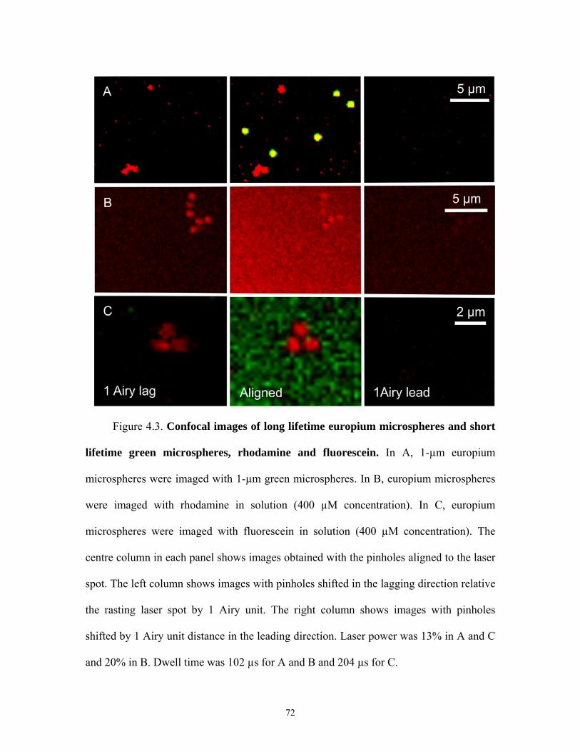
Figure 4.3. Confocal images of long lifetime europium microspheres and short

lifetime green microspheres, rhodamine and fluorescein. In A, 1-µm europium

microspheres were imaged with 1-µm green microspheres. In B, europium microspheres

were imaged with rhodamine in solution (400 µM concentration). In C, europium

microspheres were imaged with fluorescein in solution (400 µM concentration). The

centre column in each panel shows images obtained with the pinholes aligned to the laser

spot. The left column shows images with pinholes shifted in the lagging direction relative

the rasting laser spot by 1 Airy unit. The right column shows images with pinholes

shifted by 1 Airy unit distance in the leading direction. Laser power was 13% in A and C

and 20% in B. Dwell time was 102 µs for A and B and 204 µs for C.

72

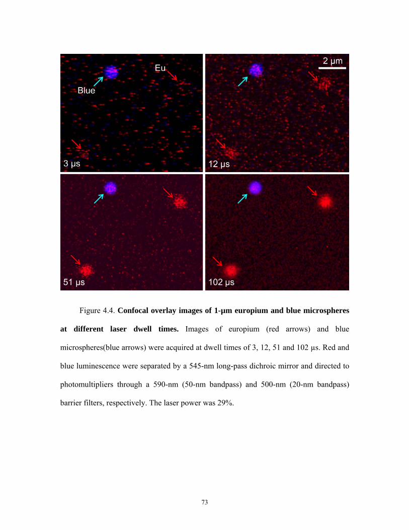
Figure 4.4. Confocal overlay images of 1-µm europium and blue microspheres

at different laser dwell times. Images of europium (red arrows) and blue

microspheres(blue arrows) were acquired at dwell times of 3, 12, 51 and 102 µs. Red and

blue luminescence were separated by a 545-nm long-pass dichroic mirror and directed to

photomultipliers through a 590-nm (50-nm bandpass) and 500-nm (20-nm bandpass)

barrier filters, respectively. The laser power was 29%.

73

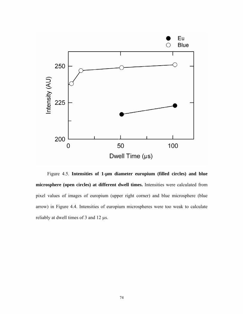
Figure 4.5. Intensities of 1-µm diameter europium (filled circles) and blue

microsphere (open circles) at different dwell times. Intensities were calculated from

pixel values of images of europium (upper right corner) and blue microsphere (blue

arrow) in Figure 4.4. Intensities of europium microspheres were too weak to calculate

reliably at dwell times of 3 and 12 µs.

74

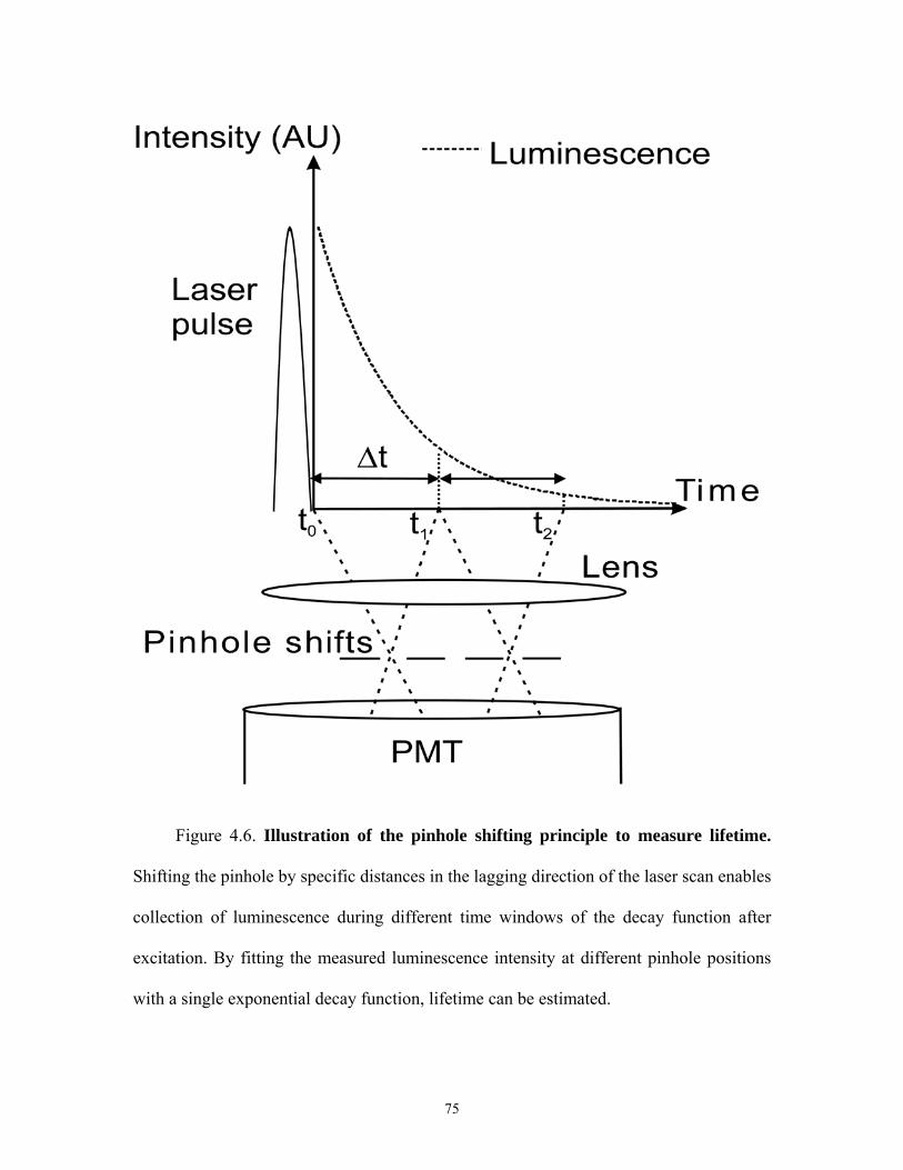
Figure 4.6. Illustration of the pinhole shifting principle to measure lifetime.

Shifting the pinhole by specific distances in the lagging direction of the laser scan enables

collection of luminescence during different time windows of the decay function after

excitation. By fitting the measured luminescence intensity at different pinhole positions

with a single exponential decay function, lifetime can be estimated.

75

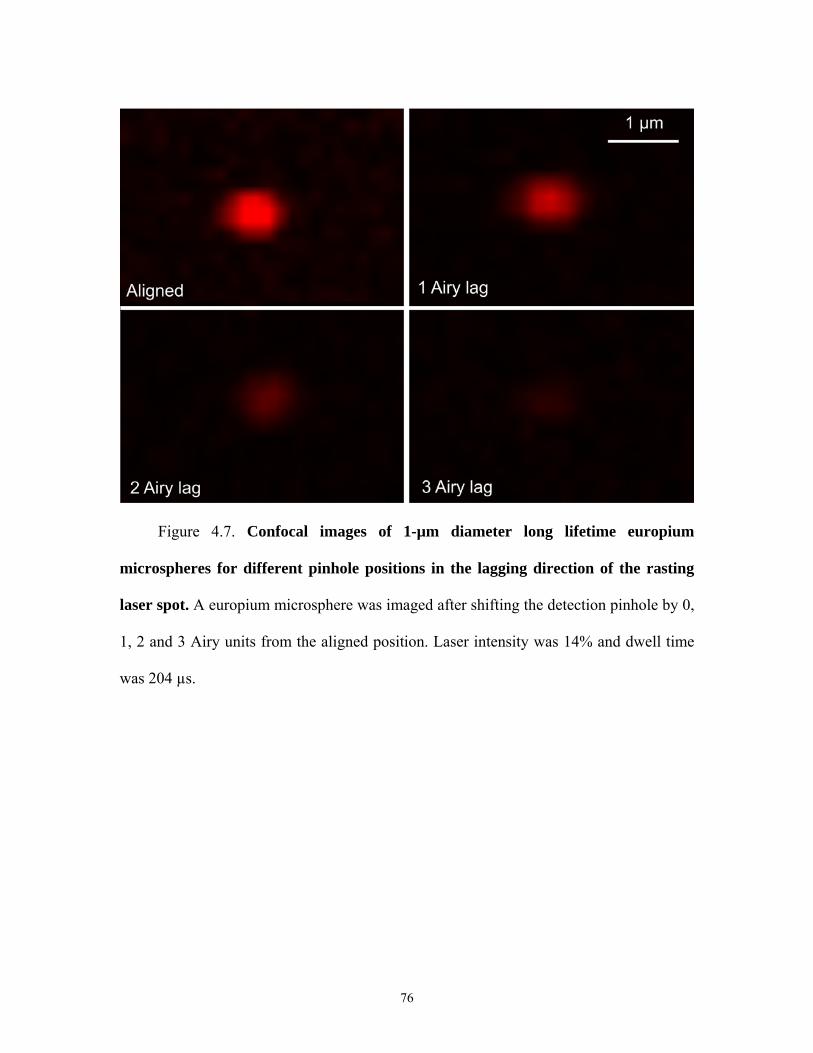
Figure 4.7. Confocal images of 1-µm diameter long lifetime europium

microspheres for different pinhole positions in the lagging direction of the rasting

laser spot. A europium microsphere was imaged after shifting the detection pinhole by 0,

1, 2 and 3 Airy units from the aligned position. Laser intensity was 14% and dwell time

was 204 µs.

76

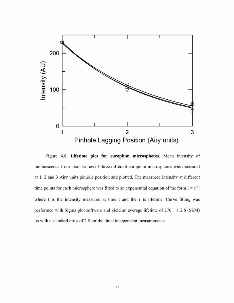
Figure 4.8. Lifetime plot for europium microspheres. Mean intensity of

luminescence from pixel values of three different europium microspheres was measured

at 1, 2 and 3 Airy units pinhole position and plotted. The measured intensity at different

time points for each microsphere was fitted to an exponential equation of the form I = e-t/τ

where I is the intensity measured at time t and the τ is lifetime. Curve fitting was

performed with Sigma plot software and yield an average lifetime of 270 �± 2.8 (SEM)

µs with a standard error of 2.8 for the three independent measurements.

77

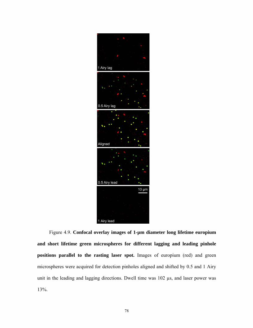
Figure 4.9. Confocal overlay images of 1-µm diameter long lifetime europium

and short lifetime green microspheres for different lagging and leading pinhole

positions parallel to the rasting laser spot. Images of europium (red) and green

microspheres were acquired for detection pinholes aligned and shifted by 0.5 and 1 Airy

unit in the leading and lagging directions. Dwell time was 102 µs, and laser power was

13%.

78

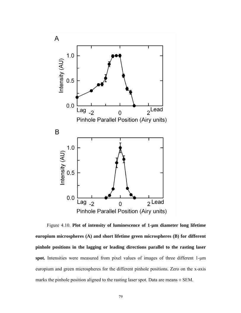
Figure 4.10. Plot of intensity of luminescence of 1-µm diameter long lifetime

europium microspheres (A) and short lifetime green microspheres (B) for different

pinhole positions in the lagging or leading directions parallel to the rasting laser

spot. Intensities were measured from pixel values of images of three different 1-μm

europium and green microspheres for the different pinhole positions. Zero on the x-axis

marks the pinhole position aligned to the rasting laser spot. Data are means ± SEM.

79

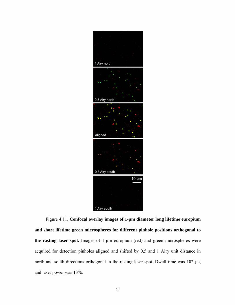
Figure 4.11. Confocal overlay images of 1-µm diameter long lifetime europium

and short lifetime green microspheres for different pinhole positions orthogonal to

the rasting laser spot. Images of 1-µm europium (red) and green microspheres were

acquired for detection pinholes aligned and shifted by 0.5 and 1 Airy unit distance in

north and south directions orthogonal to the rasting laser spot. Dwell time was 102 µs,

and laser power was 13%.

80

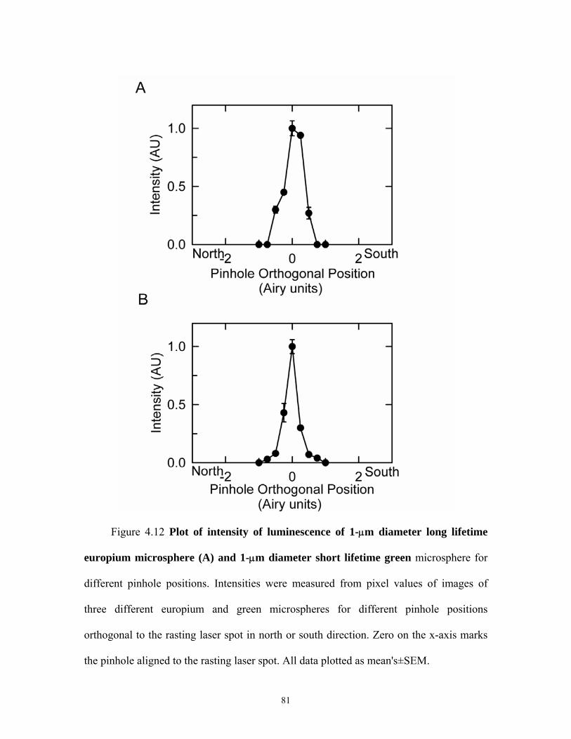
Figure 4.12 Plot of intensity of luminescence of 1-μm diameter long lifetime

europium microsphere (A) and 1-μm diameter short lifetime green microsphere for

different pinhole positions. Intensities were measured from pixel values of images of

three different europium and green microspheres for different pinhole positions

orthogonal to the rasting laser spot in north or south direction. Zero on the x-axis marks

the pinhole aligned to the rasting laser spot. All data plotted as mean's±SEM.

81

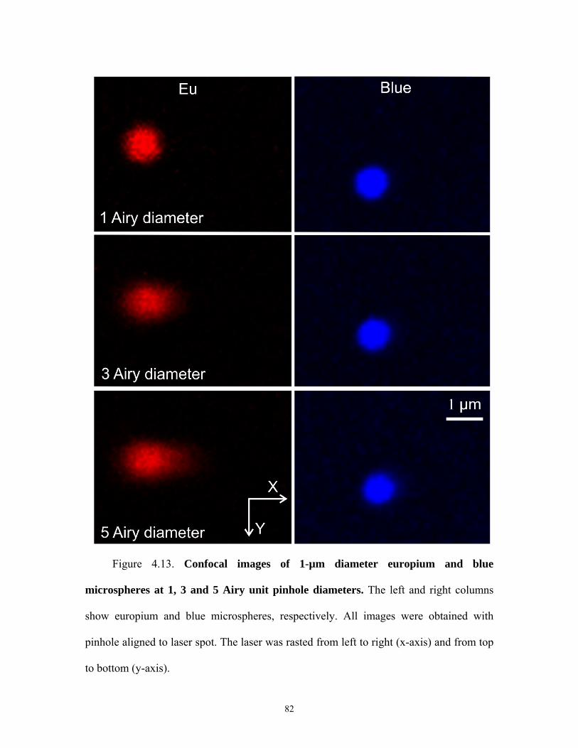
Figure 4.13. Confocal images of 1-µm diameter europium and blue

microspheres at 1, 3 and 5 Airy unit pinhole diameters. The left and right columns

show europium and blue microspheres, respectively. All images were obtained with

pinhole aligned to laser spot. The laser was rasted from left to right (x-axis) and from top

to bottom (y-axis).

82

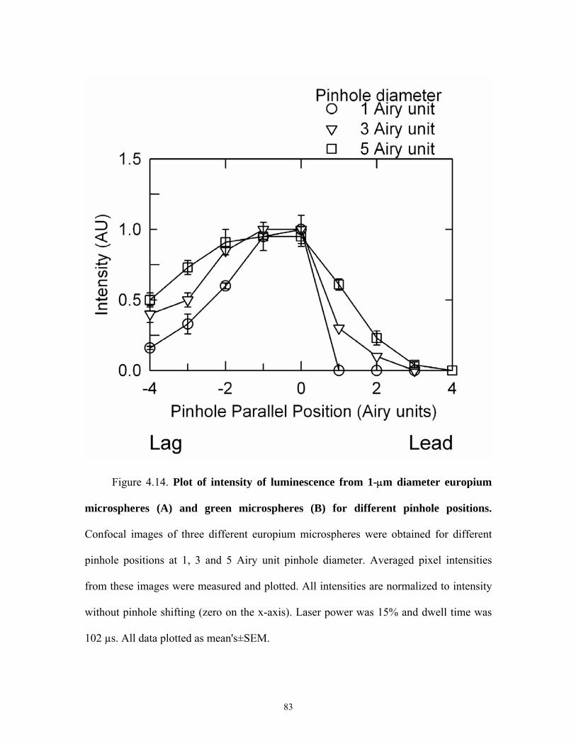
Figure 4.14. Plot of intensity of luminescence from 1-μm diameter europium

microspheres (A) and green microspheres (B) for different pinhole positions.

Confocal images of three different europium microspheres were obtained for different

pinhole positions at 1, 3 and 5 Airy unit pinhole diameter. Averaged pixel intensities

from these images were measured and plotted. All intensities are normalized to intensity

without pinhole shifting (zero on the x-axis). Laser power was 15% and dwell time was

102 µs. All data plotted as mean's±SEM.

83

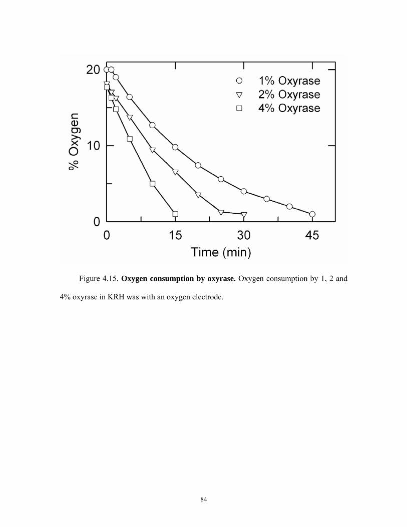
Figure 4.15. Oxygen consumption by oxyrase. Oxygen consumption by 1, 2 and

4% oxyrase in KRH was with an oxygen electrode.

84

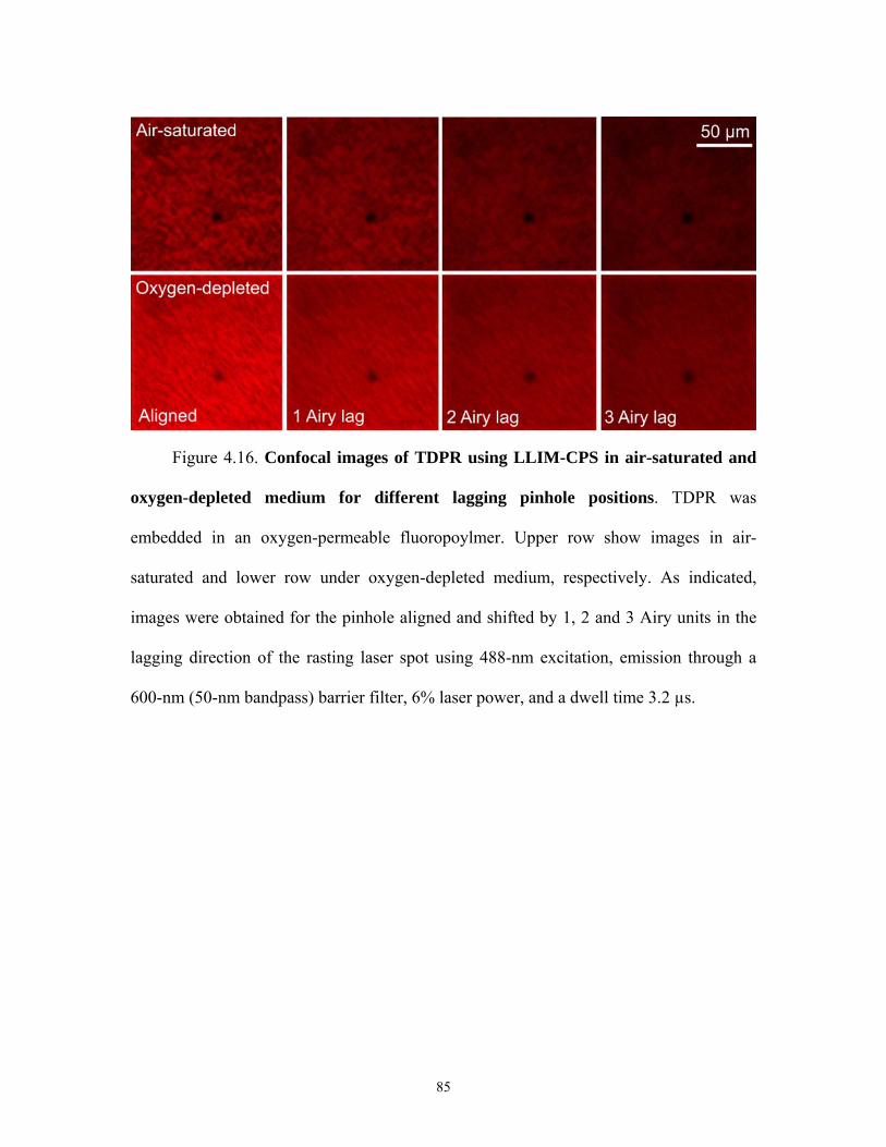
Figure 4.16. Confocal images of TDPR using LLIM-CPS in air-saturated and

oxygen-depleted medium for different lagging pinhole positions. TDPR was

embedded in an oxygen-permeable fluoropoylmer. Upper row show images in air-

saturated and lower row under oxygen-depleted medium, respectively. As indicated,

images were obtained for the pinhole aligned and shifted by 1, 2 and 3 Airy units in the

lagging direction of the rasting laser spot using 488-nm excitation, emission through a

600-nm (50-nm bandpass) barrier filter, 6% laser power, and a dwell time 3.2 µs.

85

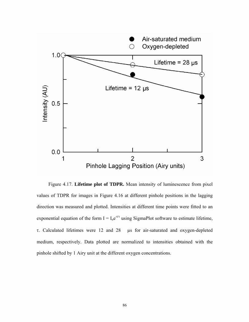
Figure 4.17. Lifetime plot of TDPR. Mean intensity of luminescence from pixel

values of TDPR for images in Figure 4.16 at different pinhole positions in the lagging

direction was measured and plotted. Intensities at different time points were fitted to an

exponential equation of the form I = Ioe-t/τ using SigmaPlot software to estimate lifetime,

τ. Calculated lifetimes were 12 and 28 �µs for air-saturated and oxygen-depleted

medium, respectively. Data plotted are normalized to intensities obtained with the

pinhole shifted by 1 Airy unit at the different oxygen concentrations.

86

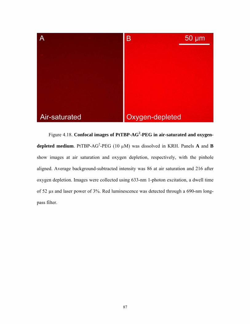
Figure 4.18. Confocal images of PtTBP-AG2-PEG in air-saturated and oxygen-

depleted medium. PtTBP-AG2-PEG (10 μM) was dissolved in KRH. Panels A and B

show images at air saturation and oxygen depletion, respectively, with the pinhole

aligned. Average background-subtracted intensity was 86 at air saturation and 216 after

oxygen depletion. Images were collected using 633-nm 1-photon excitation, a dwell time

of 52 µs and laser power of 3%. Red luminescence was detected through a 690-nm long-

pass filter.

87

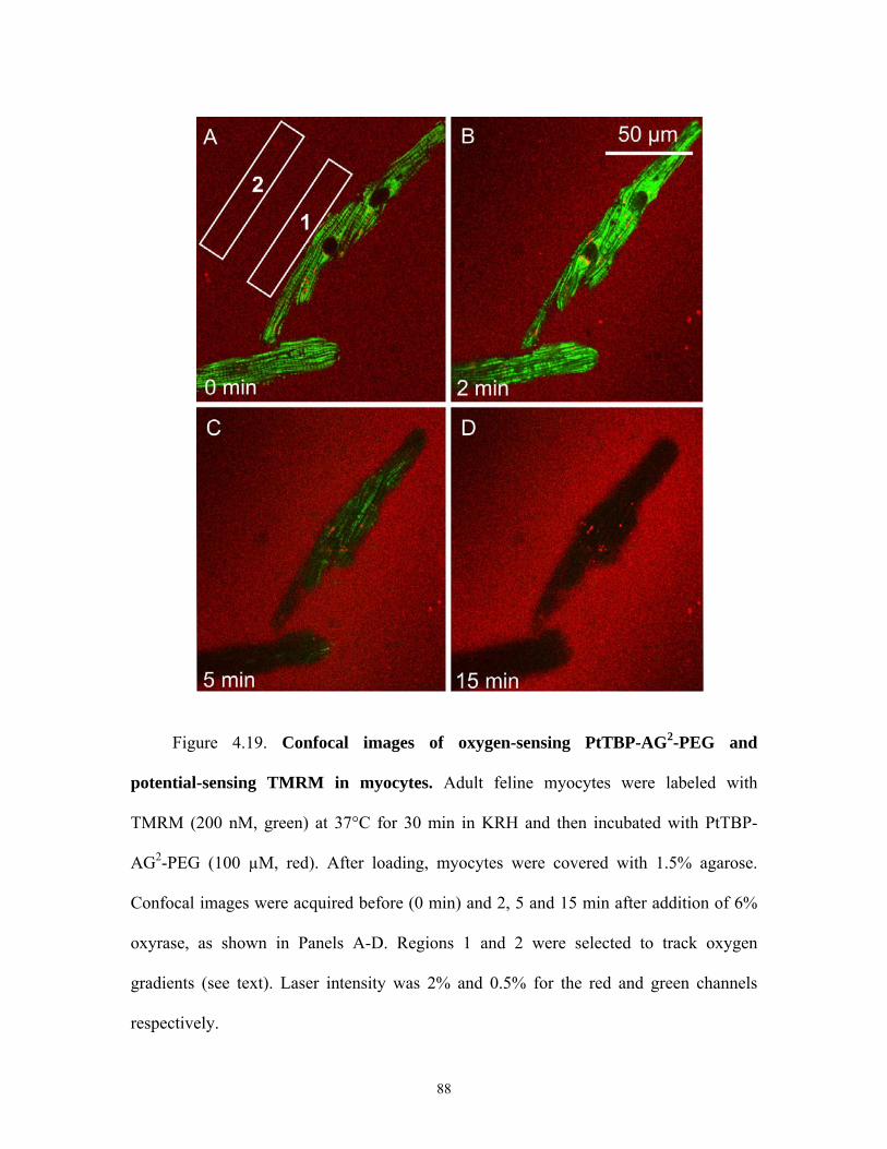
Figure 4.19. Confocal images of oxygen-sensing PtTBP-AG2-PEG and

potential-sensing TMRM in myocytes. Adult feline myocytes were labeled with

TMRM (200 nM, green) at 37°C for 30 min in KRH and then incubated with PtTBP-

AG2-PEG (100 µM, red). After loading, myocytes were covered with 1.5% agarose.

Confocal images were acquired before (0 min) and 2, 5 and 15 min after addition of 6%

oxyrase, as shown in Panels A-D. Regions 1 and 2 were selected to track oxygen

gradients (see text). Laser intensity was 2% and 0.5% for the red and green channels

respectively.

88

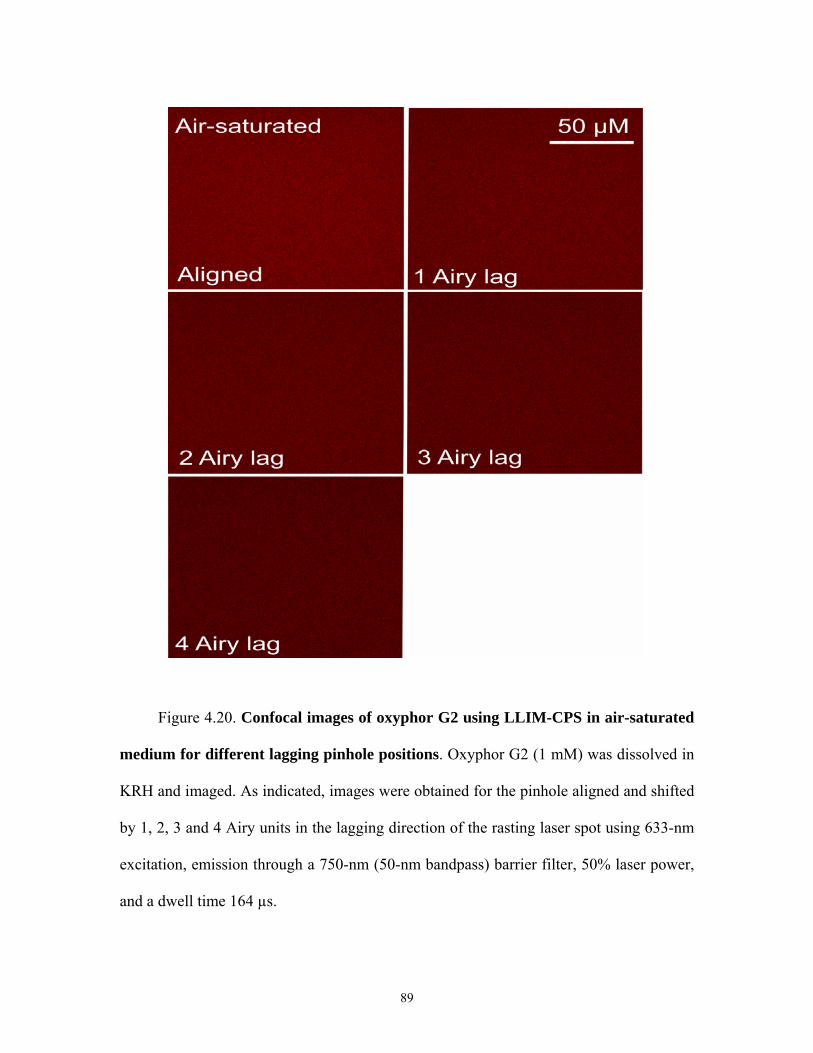
3 Airy lag

Figure 4.20. Confocal images of oxyphor G2 using LLIM-CPS in air-saturated

medium for different lagging pinhole positions. Oxyphor G2 (1 mM) was dissolved in

KRH and imaged. As indicated, images were obtained for the pinhole aligned and shifted

by 1, 2, 3 and 4 Airy units in the lagging direction of the rasting laser spot using 633-nm

excitation, emission through a 750-nm (50-nm bandpass) barrier filter, 50% laser power,

and a dwell time 164 µs.

89

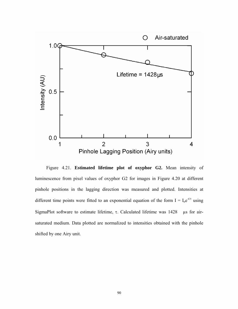
Figure 4.21. Estimated lifetime plot of oxyphor G2. Mean intensity of

luminescence from pixel values of oxyphor G2 for images in Figure 4.20 at different

pinhole positions in the lagging direction was measured and plotted. Intensities at

different time points were fitted to an exponential equation of the form I = Ioe-t/τ using

SigmaPlot software to estimate lifetime, τ. Calculated lifetime was 1428 �µs for air-

saturated medium. Data plotted are normalized to intensities obtained with the pinhole

shifted by one Airy unit.

90

CHAPTER 5

DISCUSSION

5.1 Principle of Long Lifetime Luminescence Imaging by Confocal Pinhole Shifting

Long lifetime imaging requires modifications and expensive add-ons to existing

microscopes. Here, I developed a technique of long lifetime imaging microscopy by

confocal pinhole shifting (LLIM-CPS) to perform lifetime imaging that requires no

special modification of a standard commercial laser scanning confocal/multiphoton

microscope. The principle I developed for LLIM-CPS is that when the pinhole of a

confocal microscope is shifted in the lagging direction by one Airy unit distance or more,

long lifetime luminescence becomes selectively transmitted through the pinhole, whereas

collection of short lifetime luminescence drops sharply (Figure 4.1). This expectation was

tested by experiments with europium, a long lifetime luminophore, and different short

lifetime luminophores. Shifting the pinhole in the lagging direction of the rasting laser

spot by one Airy unit distance or more caused the short lifetime luminescence of green

microspheres, rhodamine and fluorescein to disappear with retention of long lifetime

europium luminescence (Figure 4.3, left columns). Shifting in the leading direction

caused both the short and long lifetime luminescence to disappear virtually equally

(Figure 4.3, right columns). These results validate the principle of

selective long lifetime luminescence imaging by shifting the pinhole of a confocal

microscope in the lagging direction of the rasting laser spot by an Airy unit or more.

5.2 Multiphoton Excitation for Long Lifetime Imaging

Multiphoton excitation enables deeper penetration inside tissues due to the long

wavelength of the excitation light. Combined with the confinement of excitation in a

small focal volume which reduces out-of focus photo-toxicity and bleaching, multiphoton

excitability is especially useful for deep tissue imaging applications [56].

Phosphorescence-based long lifetime luminescent probes for measuring oxygen are best

excited at UV wavelengths [57]. Use of UV light increases the probability of photo-

toxicity and damage to biological structures [23]. These problems may be ameliorated by

using a multiphoton laser to excite such luminophores.

Results here showed that long lifetime luminophores like europium can be excited

with two-photon excitation for LLIM-CPS (Figure 4.2). The 720-nm wavelength selected

for europium was found to give the brightest luminescence when excited from 700 to

800-nm wavelength of the laser. The multiphoton laser (Coherent Mira 900) used for

imaging europium required manual tuning to every wavelength used, a process which

was time consuming. During the course of this work, I also found that oxygen-sensing

platinum and palladium porphyrins due to their symmetrical structure displayed lower

efficiencies of two-photon excitation than single photon excitation [58]. In my hands the

oxygen luminophore Pd-meso-tetra-(4-carboxyphenyl) porphyrin (Pdtcp) and PtTBP-

AG2-PEG did not display any two-photon excitation between the wavelengths of 700-

92

900-nm. These reasons make use of multiphoton excitation for oxygen sensing using

phosphorescent probes in living cells unfeasible.

Dr. Sergei A. Vinogradov and his group in University of Pennsylvania are currently

working on developing new oxygen luminophores which can be suitably excited with

two-photon excitation and display higher quantum efficiencies (personal

communication), [59, 60]. The development of these luminophores coupled with the

progress in computer-controlled tunable multiphoton laser technology may lead the way

for exciting work with lifetime based oxygen sensing using LLIM-CPS with multiphoton

excitation.

5.3 Effect of Dwell Time on Lifetime Imaging

Imaging of long lifetime luminophores requires selection of appropriate dwell

times. Our results show that long lifetime europium microspheres could be imaged and

clearly resolved at longer dwell times of 51 and 102 µs because of the weakness of the

signal at shorter dwells (Figure 4.4) At shorter dwell times of 3 and 12 µs the images

were grainy with the inability to clearly resolve the europium microspheres. For short

lifetime microspheres, mean intensity did not change as dwell time increased. Thus,

fluorescence of short lifetime blue microspheres was independent of dwell times and

could be resolved even at the shortest dwell time of 3 µs (Figure 4.5).

Use of longer dwell times resulted in longer light exposures which became a

problem for live cell imaging where phototoxicity and bleaching was a concern. Oxygen

quenches long lifetime oxygen-sensing luminophores, which results in generation of

93

singlet oxygen and phototoxicity [61]. The amount of singlet oxygen generated is

proportional to light exposure. Judicious choice of light exposure is critical for

maintaining the viability of cells and yet obtaining adequate S/N ratio in experiments of

live cell imaging with LLIM-CPS.

5.4 Measuring Lifetimes

Using LLIM-CPS and shifting the pinhole by different distances, I could measure

the luminescence during different windows of decay (Equations 4.2 and 4.3 and Figure

4.6). Images of luminescence were acquired for three different lagging pinhole positions

for europium microspheres (Figure 4.7). Intensity measured from the pixel values was

plotted against the time of measurement, and lifetime was estimated by fitting the

measurement with a single exponential decay function. Using this technique, lifetime of

europium microspheres was measured as an average of 270 ± 2.8 (SEM) µs from three

independent measurements (Figure 4.8).

While this result showed that lifetimes on the order of several hundred

microseconds and possibly longer can be measured with LLIM-CPS, the shortest lifetime

that can be measured using pinhole shifting is limited by the speed/dwell time of the

rasting laser spot. Measurement of lifetime requires at least two windows of

measurement, namely two shifted pinhole positions. In LLIM-CPS, each window of

measurement is equal to the dwell time of the rasting laser spot. The shortest available

dwell time for LLIM-CPS is 1 µs. Based on these conditions the shortest possible

measurable lifetime using LLIM-CPS is about 1 µs. Development of faster scanning

94

technologies, such as acousto-optic scanning, will decrease the dwell times and hence

may allow shorter lifetimes to be measured in the future by using LLIM-CPS.

5.5 Quantification of Pinhole Shifting

Quantification of pinhole shifting distances for long lifetime imaging was

performed with europium and green microspheres. In the lagging direction, europium

microspheres lost their luminescence more slowly than in the leading direction. A pinhole

shift of 1 Airy unit distance (physical distance of 110 µm) retained 45% of luminescence

compared to a one Airy unit pinhole shift in the leading direction at which point virtually

all luminescence was lost (Figure 4.9 and 4.10A) Even a pinhole shift of 3 Airy units

(physical shift distance of ~330 µm) in the lagging direction retained about 15% of the

luminescence. For short lifetime green microspheres, all luminescence was lost at a

pinhole shift of one Airy unit distance in either the lagging or leading direction (Figure

4.9 and 4.10B). These results support the theoretical prediction that pinhole shifts of one

Airy unit distance or more in the lagging direction selectively image long lifetime

luminescence.

Quantification of pinhole positioning is essential for imaging lifetimes as one needs

to be accurate in shifting and positioning the pinhole to collect different lifetimes.

Improper pinhole shifting will cause errors in the measurement of the lifetimes. Also, a

shift as small as 0.25 Airy units caused some loss of luminescence from short lifetime

green microspheres (Figure 4.10B). Accuracy of pinhole positioning is thus needed to

95

align precisely the pinhole with respect to the rasting laser spot for most efficient

collection of short lifetime fluorescence.

Our results from pinhole shifting in the orthogonal direction showed that both long

lifetime europium and short lifetime green luminescence disappeared in a virtually

identical fashion in both the north and south orthogonal directions. Luminescence fell off

rapidly in orthogonal directions with virtually complete disappearance within a single

Airy unit distance pinhole shift (Figures 4.11 and 4.12). Thus, only by shifting the

pinhole in the lagging direction parallel to the rasting laser spot can long lifetime

luminescence be selectively imaged.

5.6 Effect of Pinhole Diameter on Lifetime Imaging

Collection of long lifetime luminescence for pinhole diameters larger than one Airy

unit caused asymmetric distortions in the images of the long lifetime europium (Figure

4.13). Increasing the pinhole diameter allowed collection of delayed luminescence

simultaneously with the short lifetime luminescence without shifting the pinhole.

However, the short and long lifetime luminescence that simultaneously passes through

the pinhole will come from different parts of the specimen. Thus, collection of delayed

luminescence with pinhole diameters greater than 1 Airy unit will cause distortions in the

images of long lifetime specimens. Microspheres displayed a diameter greater than their

true diameter of 1-µm in the x-direction with the diameter increasing to 1.5 and 2.0 µm

with 3 and 5 Airy unit pinhole diameters. Nonetheless, at a pinhole diameter of one Airy

unit, long lifetime europium microspheres were resolved to their true diameter.

96

With increasing pinhole diameter, greater lateral shifting of the pinhole was

required to remove overlap of the pinhole with the projection of the laser crossover spot

as an Airy disk onto the pinhole image plane. For example, the pinhole needed to be

shifted by 2 and 3 Airy units distance for 3 and 5 Airy unit pinhole diameters,

respectively, to remove this overlap (Figure 4.14). Thus, use of greater pinhole diameters

for selectively imaging long lifetimes by LLIM-CPS is possible only by using increasing

pinhole shifts. Use of pinhole diameters greater than one Airy unit allows collection of

luminescence originating from regions above and below the plane of focus thereby

increasing the collected signal, although axial resolution is degraded. A compromise of

axial resolution by increasing pinhole diameter may be beneficial for live cell imaging

with long lifetime luminophores whose quantum efficiencies are lower than short lifetime

fluorophores. Although distortions in long lifetime luminescence images occur with

pinhole diameters of greater than one Airy unit, software adjustments to the correct such

distortions can be explored to correct for these aberrations.

5.7 Imaging of the Long Lifetime Oxygen Luminophore tris-4, 7 diphenyl 1, 10-

phenanthroline ruthenium

Using LLIM-CPS, I imaged the intensity and lifetime of TDPR under different

oxygen concentrations. This luminophore is quenched by oxygen and has been used

previously to monitor oxygen by intravital microscopy in the intensity domain [54]. In

my hands, TDPR exhibited an increase in intensity by a factor of 1.7 when exposed to

97

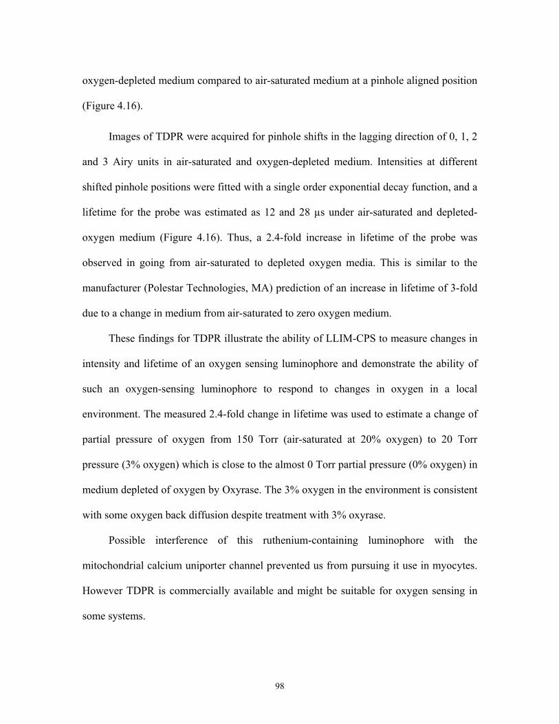
oxygen-depleted medium compared to air-saturated medium at a pinhole aligned position

(Figure 4.16).

Images of TDPR were acquired for pinhole shifts in the lagging direction of 0, 1, 2

and 3 Airy units in air-saturated and oxygen-depleted medium. Intensities at different

shifted pinhole positions were fitted with a single order exponential decay function, and a

lifetime for the probe was estimated as 12 and 28 µs under air-saturated and depleted-

oxygen medium (Figure 4.16). Thus, a 2.4-fold increase in lifetime of the probe was

observed in going from air-saturated to depleted oxygen media. This is similar to the

manufacturer (Polestar Technologies, MA) prediction of an increase in lifetime of 3-fold

due to a change in medium from air-saturated to zero oxygen medium.

These findings for TDPR illustrate the ability of LLIM-CPS to measure changes in

intensity and lifetime of an oxygen sensing luminophore and demonstrate the ability of

such an oxygen-sensing luminophore to respond to changes in oxygen in a local

environment. The measured 2.4-fold change in lifetime was used to estimate a change of

partial pressure of oxygen from 150 Torr (air-saturated at 20% oxygen) to 20 Torr

pressure (3% oxygen) which is close to the almost 0 Torr partial pressure (0% oxygen) in

medium depleted of oxygen by Oxyrase. The 3% oxygen in the environment is consistent

with some oxygen back diffusion despite treatment with 3% oxyrase.

Possible interference of this ruthenium-containing luminophore with the

mitochondrial calcium uniporter channel prevented us from pursuing it use in myocytes.

However TDPR is commercially available and might be suitable for oxygen sensing in

some systems.

98

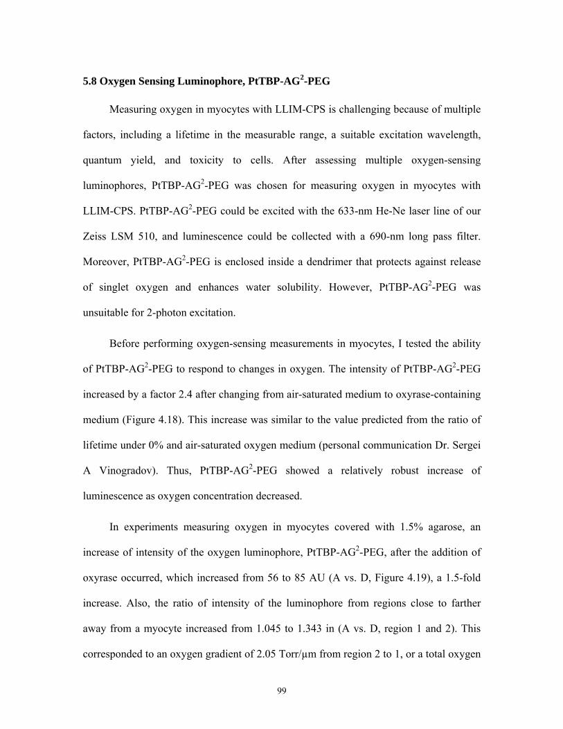
5.8 Oxygen Sensing Luminophore, PtTBP-AG2-PEG

Measuring oxygen in myocytes with LLIM-CPS is challenging because of multiple

factors, including a lifetime in the measurable range, a suitable excitation wavelength,

quantum yield, and toxicity to cells. After assessing multiple oxygen-sensing

luminophores, PtTBP-AG2-PEG was chosen for measuring oxygen in myocytes with

LLIM-CPS. PtTBP-AG2-PEG could be excited with the 633-nm He-Ne laser line of our

Zeiss LSM 510, and luminescence could be collected with a 690-nm long pass filter.

Moreover, PtTBP-AG2-PEG is enclosed inside a dendrimer that protects against release

of singlet oxygen and enhances water solubility. However, PtTBP-AG2-PEG was

unsuitable for 2-photon excitation.

Before performing oxygen-sensing measurements in myocytes, I tested the ability

of PtTBP-AG2-PEG to respond to changes in oxygen. The intensity of PtTBP-AG2-PEG

increased by a factor 2.4 after changing from air-saturated medium to oxyrase-containing

medium (Figure 4.18). This increase was similar to the value predicted from the ratio of

lifetime under 0% and air-saturated oxygen medium (personal communication Dr. Sergei

A Vinogradov). Thus, PtTBP-AG2-PEG showed a relatively robust increase of

luminescence as oxygen concentration decreased.

In experiments measuring oxygen in myocytes covered with 1.5% agarose, an

increase of intensity of the oxygen luminophore, PtTBP-AG2-PEG, after the addition of

oxyrase occurred, which increased from 56 to 85 AU (A vs. D, Figure 4.19), a 1.5-fold

increase. Also, the ratio of intensity of the luminophore from regions close to farther

away from a myocyte increased from 1.045 to 1.343 in (A vs. D, region 1 and 2). This

corresponded to an oxygen gradient of 2.05 Torr/µm from region 2 to 1, or a total oxygen

99

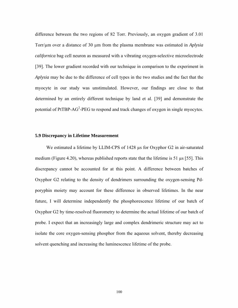
difference between the two regions of 82 Torr. Previously, an oxygen gradient of 3.01

Torr/µm over a distance of 30 µm from the plasma membrane was estimated in Aplysia

californica bag cell neuron as measured with a vibrating oxygen-selective microelectrode

[39]. The lower gradient recorded with our technique in comparison to the experiment in

Aplysia may be due to the difference of cell types in the two studies and the fact that the

myocyte in our study was unstimulated. However, our findings are close to that

determined by an entirely different technique by land et al. [39] and demonstrate the

potential of PtTBP-AG2-PEG to respond and track changes of oxygen in single myocytes.

5.9 Discrepancy in Lifetime Measurement

We estimated a lifetime by LLIM-CPS of 1428 µs for Oxyphor G2 in air-saturated

medium (Figure 4.20), whereas published reports state that the lifetime is 51 µs [55]. This

discrepancy cannot be accounted for at this point. A difference between batches of

Oxyphor G2 relating to the density of dendrimers surrounding the oxygen-sensing Pd-

poryphin moiety may account for these difference in observed lifetimes. In the near

future, I will determine independently the phosphorescence lifetime of our batch of

Oxyphor G2 by time-resolved fluorometry to determine the actual lifetime of our batch of

probe. I expect that an increasingly large and complex dendrimeric structure may act to

isolate the core oxygen-sensing phosphor from the aqueous solvent, thereby decreasing

solvent quenching and increasing the luminescence lifetime of the probe.

100

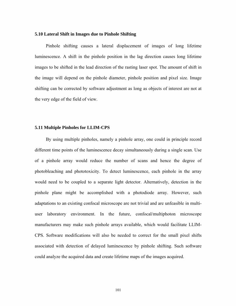
5.10 Lateral Shift in Images due to Pinhole Shifting

Pinhole shifting causes a lateral displacement of images of long lifetime

luminescence. A shift in the pinhole position in the lag direction causes long lifetime

images to be shifted in the lead direction of the rasting laser spot. The amount of shift in

the image will depend on the pinhole diameter, pinhole position and pixel size. Image

shifting can be corrected by software adjustment as long as objects of interest are not at

the very edge of the field of view.

5.11 Multiple Pinholes for LLIM-CPS

By using multiple pinholes, namely a pinhole array, one could in principle record

different time points of the luminescence decay simultaneously during a single scan. Use

of a pinhole array would reduce the number of scans and hence the degree of

photobleaching and phototoxicity. To detect luminescence, each pinhole in the array

would need to be coupled to a separate light detector. Alternatively, detection in the

pinhole plane might be accomplished with a photodiode array. However, such

adaptations to an existing confocal microscope are not trivial and are unfeasible in multi-

user laboratory environment. In the future, confocal/multiphoton microscope

manufacturers may make such pinhole arrays available, which would facilitate LLIM-

CPS. Software modifications will also be needed to correct for the small pixel shifts

associated with detection of delayed luminescence by pinhole shifting. Such software

could analyze the acquired data and create lifetime maps of the images acquired.

101

Light detected simultaneously from multiple pinholes can also be used to ratio

signals acquired at different pinhole positions as a measure of the amount of delayed

luminescence. Advantages of ratioing include an automatic correction for fluctuations in

laser intensity and variations in probe concentrations.

5.12 Comparison with other Lifetime Techniques

Lifetime measurements that use wide field imaging lack the ability to resolve sub

micron structures. Lifetime imaging using confocal microscopes and multiphoton lasers

enable imaging of sub-micron structures [8, 29]. Such systems require expensive

equipment to be added to the basic confocal/multiphoton microscope to adapt the

instrumentation to perform lifetime imaging [11]. Moreover, most such systems (time or

frequency based systems) are adapted to measure lifetimes on the nanosecond time scale

and cannot be used to measure lifetimes of more than about 1 µs [12]. Thus, these

instrumentation are unsuitable to monitor long life time probes like oxygen-sensing

fluorophores for study of oxygen uptake in cardiac myocytes and other cell types.

LLIM-CPS using a confocal multiphoton system provided submicron resolution

enabling measurement of lifetimes at sub-cellular resolution. LLIM-CPS was based on

the simple technique of shifting the pinhole of an existing confocal microscope. Thus,

LLIM-CPS does not require extensive modifications or expensive add-on equipment to

the basic confocal/multiphoton system. The range of lifetimes that can be measured with

LLIM-CPS ranges from about 1 µs to several hundred microseconds, a range that

includes most of the oxygen sensing luminophores. The wavelength tunability of a

102

multiphoton lasers (typically 700-1000-nm) coupled with development of multiphoton

excitable oxygen sensing probes should allow practical oxygen imaging of liver cells in

the future.

Some studies have already implemented luminescence based lifetime imaging to

sense oxygen at the cellular level in non-cardiac cells [61, 62, 63]. However, these

systems used either custom built lifetime imaging apparatus or extensive (and expensive)

modifications to existing microscopes to perform the measurements. Our system

described here shows the ability to measure oxygen gradients in heart cells non-

invasively using a luminescence based technique without any modification to the

confocal microscope. This technique allows one to make quantitative estimates of oxygen

concentration gradients near heart cells based on the intensity and/or lifetime of oxygen-

sensing luminophore.

5.13 Drawbacks of LLIM-CPS

The main drawback to LLIM-CPS is speed, since the luminophore signals from

each pixel are acquired on a pixel by pixel basis and hence significant time is spent in

acquiring an entire image (typically 512x512). Since long lifetime luminophores exhibit

lower quantum efficiencies, more power and longer exposures are required to collect

enough photons for an adequate S/N, which further increases the acquisition time. Also,

images have to be acquired for two or more pinhole shift positions resulting in longer

imaging times. Lifetime systems using CCD and streak cameras with point scanners

enable faster lifetime imaging of the specimen since they collect an image from all the

103

pixels in the image simultaneously or collect the entire luminescence decay from each

pixel during a single exposure [5, 64].

5.14 Conclusions

I have shown here the ability of an existing confocal microscope to perform

lifetime imaging. By shifting the detection pinhole of the confocal microscope in the

lagging direction parallel to the laser scan, long lifetime luminescence can be selectively

imaged. I call this technique luminescence lifetime imaging microscopy by confocal

pinhole shifting (LLIM-CPS). Using LLIM-CPS, the lifetime of europium was measured

as 270 µs, similar to previously reported values. Further by using LLIM-CPS, I could

show an oxygen dependent change in lifetime and intensity of oxygen luminophore

TDPR. To my knowledge this is the first time that the principle of LLIM-CPS has been

proposed and experimentally validated.

A goal of LLIM-CPS was to measure oxygen concentrations. I showed here the

suitability of using the oxygen-sensing luminophore, PtTBP-AG2-PEG to visualize

oxygen using LLIM-CPS and illustrate the ability of the luminophore to track changes in

oxygen in the intensity domain. These results demonstrate that oxygen can be measured

around a heart cell by using oxygen-dependent quenching of a phosphorescent probe.

Future work can build upon the existing knowledge from this project and complete the

goal of correlating calcium transients with oxygen uptake in myocytes and add further

evidence to the regulation of mitochondrial metabolism by calcium. While my project

focused on the use of LLIM-CPS on sensing oxygen, use of this technique is not limited

104

to oxygen imaging. LLIM-CPS for imaging other ions like calcium, pH and techniques

like fluorescence resonance energy transfer with LLIM-CPS may also be possible.

Commercial implementation of LLIM-CPS on confocal microscopes in the future

needs to be investigated. Implementation of this technique on commercial laser scanning

confocal microscopes will involve using multiple pinholes, fitting of suitable beam

splitters and emission filters, addition of excitation lasers matched to the desired long

lifetime luminophore, and creation of software to automate the measurements. Also,

development of additional probes which can be used with LLIM-CPS for different

application needs to be pursued.

105

REFERENCES

1. V. K. Ramanujan, J.-H. Zhang, E. Biener and B. Herman, "Multiphoton fluorescence lifetime contrast in deep tissue imaging: prospects in redox imaging and disease diagnosis," Journal of Biomedical Optics 10, (2005). 2. B. J. Muller-Borer, H. Yang, S. A. M. Marzouk, J. J. Lemasters and W. E. Cascio, "pHi and pHo at different depths in perfused myocardium measured by confocal fluorescence microscopy," American Journal of Physiology - Heart and Circulatory Physiology 275, H1937-1947 (1998). 3. B. S. Launikonis, J. Zhou, L. Royer, T. R. Shannon, G. Brum and E. Ríos, "Confocal imaging of [Ca2+] in cellular organelles by SEER, shifted excitation and emission ratioing of fluorescence," Journal of Physiology 567, 523-543 (2005). 4. S. Smiley, M. Reers, C. Mottola-Hartshorn, M. Lin, A. Chen, T. Smith, G. D. Steele Jr and L. Chen, "Intracellular heterogeneity in mitochondrial membrane potentials revealed by a J-aggregate- forming liophilic cation JC-1," Proceedings of National Academy of Sciences 88, 3671-3675 (1991). 5. A. Periasamy, P. Wodnicki, X. F. Wang, S. Kwon, G. W. Gordon and B. Herman, "Time-resolved fluorescence lifetime imaging microscopy using a picosecond tunable dye laser system," Review of Scientific Instruments 67, 3722-3731 (1996). 6. A. Draaijer, R. Sanders and H. C. Gerritsen, "Fluorescence lifetime imaging, a new tool in confocal microscopy," in Handbook of Biological Confocal Microscopy, J. B. Pawley, Ed., pp. 491-505, 2nd ed. New York: Plenum Press, 1995. 7. H. Szmacinski, J. R. Lakowicz and M. L. Johnson, "Fluorescence lifetime imaging microscopy: homodyne technique using high-speed gated image intensifier," Methods in Enzymology 240, 723-748 (1994). 8. C. J. D. Grauw and H. C. Gerritsen, "Multiple time-gated module for fluorescence lifetime imaging," Applied Spectroscopy 55, 670-678 (2001). 9. P. I. H. Bastiaens and A. Squire, "Fluorescence lifetime imaging microscopy: spatial resolution of biochemical processes in the cell," Trends in Cell Biology 9, 48-52 (1999).

106

10. D. F. Wilson, W. L. Rumsey, T. J. Green and J. M. Vanderkooi, "The oxygen dependence of mitochondrial oxidative phosphorylation measured by a new optical method for measuring oxygen concentration," The Journal of Biological Chemistry 263, 2712-2718 (1987). 11. D. Elson, J. Requejo-Isidro, I. Munro, F. Reavell, J. Siegel, K. Suhling, P. Tadrous and P. French, "Time-domain fluorescence lifetime imaging applied to biological tissue," Photochemistry and Photobiology 3, 795-801 (2004). 12. W. Zhong, P. Urayama and M.-A. Mycek, "Imaging fluorescence lifetime modulation of a ruthenium-based dye in living cells: the potential for oxygen sensing," Journal of Physics D: Applied Physics 36, 1689-1695 (2003). 13. J. J. Lemasters, "Fluoresecence imaging microscopy," in Encyclopedia of Analytical Chemistry, R. A. Meyers, Ed., pp. 10351-10364. Chichester: John Wiley & Sons Ltd, 2000. 14. T. Wilson, "Confocal microscopy: Basic principles and architectures," in Confocal and Two-Photon Microscopy Foundations, Applications, and Advances, A. Diaspro, Ed., pp. 19-38. New York: Wiley-Liss, Inc., 2002. 15. A. Boyde, "Marvin Minsky, "Memoir on inventing the confocal scanning mucroscope,"" Scanning 10, 128-138 (1988). 16. D. B. Murphy, Fundamentals of Light Microscopy and Electronic Imaging: John Wiley & Sons, Inc., 2001. 17. T.Tanaami, S.Otsuki, N.Tomosada, Y.Kosugi, M.Shimizu and H.Ishida, "High Speed 1-frame/ms scanning confocal microscope with a miclolens and Nipkow disks," Applied Optics 41, (2002). 18. J. E. N. Jonkman and E. H. K. Stelzer, "Resolution and contrast in confocal and two-photon microscopy," in Confocal and Two-Photon Microscopy, A. Diaspro, Ed., pp. 101-125. NY: Wiley-Liss, Inc., 2002. 19. G. M. Maria, "Uber Elementarakte mit zwei Quantensprungen," Annals of Physics 9, 273-295 (1931).

107

20. W. Denk, J. H. Strikler and W. Web, "Two-photon laser scanning fluorescence microscopy," Science 248, 73-76 (1990). 21. A. Diaspro and C. J. Sheppard, "Two-Photon excitation fluorescence microscopy," in Confocal and Two-Photon Microscopy Foundations, Applications and Advances, A. Diaspro, Ed., pp. 39-73. NY: Wiley-Liss, 2002. 22. W. R. Zipfel, R. M. Williams and W. W. Webb, "Nonlinear magic: multiphoton microscopy in the biosciences," Nature Biotechnology 11, 1369-1377 (2003). 23. D. W. Piston, "Imaging living cells and tissues by two-photon excitation microscopy," Trends in Cell Biology 9, (1999). 24. J. R. Lakowicz, Principles of Fluorescence Spectroscopy, New York, 1986. 25. P. J. Tadrous, "Methods for imaging the structure and function of living tissues and cells: 2. Fluorescence lifetime imaging," The Journal of Pathology 191, 229-234 (2000). 26. C. Morgan, A. Mitchell and J. Murray, "Nanosesond time-resolved fluorescence microscopy: Principles and practice," Trans R Microsc Society 1, 463-466 (1990). 27. J. R. Lakowicz, H. Szmacinski and K. Nowaczyk, "Fluorescence Lifetime Imaging," Proceedings of National Academy of Sciences 89, 1271-1275 (1992). 28. T. Ni and L. Melton, "Fluorescence lifetime imaging: An approach for fuel equivalence ratio imaging," Applied Spectroscopy 45, 938-943 (1992). 29. E. P. Buurman, P. Sanders, A. Draaijer, H. C. Gerritsen, J. J. F. Van Venn, P. M. Houpt and y. K. Levine, "Fluorescence lifetime imaging using a confocal microscope," Scanning 14, 155-159 (1992). 30. H. C. Gerritsen, M. A. H. Asselbergs, A. V. Agronskaia and W. G. J. H. M. Van Sark, "Fluorescence lifetime imaging in scanning microscopes: Acquisition speed, photon economy and lifetime resolution," Journal of Microscopy 206, 218-224 (2002).

108

31. R. M. Ballew and J. N. Demas, "An error analysis of the rapid lifetime determination Method for the evaluation of single exponential decays," Analytical Chemistry 61, 30-33 (1989). 32. J. R. Lakowicz, Topics in Fluorescence Spectroscopy: Plenum Press. 33. E. Gratton and M. Limkeman, "A continuosly variable frequency cross-correlation phase fluorometer with picosecond resolution," Biophysical Journal 44, 315-324 (1983). 34. J. N. Demas, B. A. Degraff and P. B. Coleman, "Oxygen sensors based on luminescence quenching," Analytical Chemistry 71, 793A-800A (1999). 35. E. M. Brumberg, "Fluorescence microscopy of biological objects using light from above," Biophysics 4, 97-104 (1959). 36. Z. Lin, "Time-Resolved Fluorescence-Based Europium-Derived Probes for peroxidase bioassays, citrate cycle imaging and chirality sensing," Department of Chemistry and Pharmacy, 130 (2004). 37. E. Takahashi, K. Sato, H. Endoh, Z.-l. Xu and K. Doi, "Direct observation of radial intracellular PO2 gradients in a single cardiomyocyte of the rat," American Journal of Physiology - Heart and Circulatory Physiology 275, H225-H233 (1998). 38. D.Y. Yu and S. J. Cringle, "Oxygen Distribution in the mouse retina," Investigative Opthamology and Visual Science 47, 1109-1112 (2006). 39. S. C. Land, D. M. PorterField, R. H. Sanger and P. J. Smith, "The self-referencing oxygen-selective microelectrode: detection of transmembrane oxygen flux from single cells," Journal of Experimental Biology 202, 211-218 (1999). 40. G. Zaharchuk, R. Busse, G. Rosenthal, G. Manley, O. Glenn and W. Dillon, "Noninvasive oxygen partial pressure measurement of human body fluids in vivo using magnetic resonance imaging," Academic Radiology 13, 1016-1024 (2006).

109

41. J. G. McCormack and R. M. Denton, "The effects of cacium ions and adenine nucleotides on the activity of pig heart 2-oxoglutarate dehydrogenase complex," Biochemical Journal 180, 533-544 (1979). 42. J. R. Williamson and R. H. Cooper, "Regulation of the citric acid cycle in mammalian systems," FEBS letters 117 (Suppl.), K73-K85 (1980). 43. L. Buntinas, K. K. Gunter, G. C. Sparagna and T. E. Gunter, "The rapid mode of calcium uptake into heart mitochondria (RaM): comparison to RaM in liver mitochondria," Biochimica Et Biophysica Acta 1504, 248-261 (2001). 44. D. R. Trollinger, W. E. Cascio and J. J. Lemasters, "Mitochondrial calcium transients in adult rabbit cardiac myocytes: Inhibition by ruthenium red and artifacts caused by lysosomal loading of Ca2+ indicating fluorophores," Biophysical Journal 79, 39-50 (2000). 45. M. F. Gallitelli, M. Schultz, G. Isenberg and F. Rudolf, "Twitch-potential increases calcium in peripheral more than central mitochondria of guinea-pig ventricular myocytes," Journal of Physiology (London) 518, 433-447 (1999). 46. D. R. Trollinger, W. E. Cascio and J. J. Lemasters, "Selective loading of Rhod 2 into mitochondria shows mitochondrial Ca2+ transients during the contractile cycle in adult rabbit cardiac myocytes," Biochemical Research Communication 236, 738-742 (1997). 47. H. Miyata, H. S. Silverman, S. J. Sollott, E. G. Lakatta, M. D. Stern and H. R.G., "Measurement of mitochondrial free Ca2+ contraction in living single rat cardiac myocytes," American Journal of Physiology 261, H1123-H1134 (1991). 48. E. J. Griffiths, M. D. Stern and H. S. Silverman, "Measurement of mitochondrial calcium in single living cardiac myocytes by selective removal of cytosolic Indo 1," American Journal of Physiology 273, C37-C44 (1997). 49. R. Rizzuto, A. W. M. Simpson, M. Brini and T. Pozzan, "Rapid changes of mitochondrial Ca2+ revealed by specifically targeted recombinant aequorion," Nature 358, 325-332 (1992).

110

50. E. Chacon, H. Ohata, I. S. Harper, D. R. Trollinger, B. Herman and J. J. Lemasters, "Mitochondrial free calcium transients during excitation-contraction in rabbit cardiac myocytes," FEBS letters 382, 31-36 (1996). 51. H. Ohata, E. Chacon, S. A. Tesfai, B. Herman and J. J. Lemasters, "Mitochondrial Ca2+ transients in cardiac myocytes during excitation-contraction cycle: effects of pacing and hormonal stimulation," Journal of Bioenergetics and Biomembranes 30, 207-222 (1998). 52. S. Kato, C. T. Ivester, G. Cooper. IV, M. R. Zile and P. J. Mcdermott, "Growth effects of electrically stimulated contraction on adult feline cardiomyocytes in primary culture," American Journal of Physiology 37, H2495-H2504 (1994). 53. R. P. Haugland, Handbook of Fluorescent Probes and Research Products, 9 ed: Molecular Probes, Inc., 2002. 54. M. Paxian, S. A. Keller, B. Cross, T. T. Huynh and M. G. Clemens, "High-resolution visualization of oxygen distribution in the liver in vivo," American Journal of Gastrointestinal and Liver Physiology 286, G37-G44 (2004). 55. I. Dunphy, S. A. Vinogradov and D. F. Wilson, "Oxyphor R2 and G2: phosphors for measuring oxygen by oxygen-dependent quenching of phosphorescence," Analytical Biochemistry 310, 191-198 (2002). 56. A. Diaspro, M. Corosu, P. Ramoino and M. Robello, "Two-Photon excitation imaging based on a compact scanning head," IEEE Engineering in Medicine and Biology Magazine 18 18-30 (1999). 57. D. B. Papkovsky and T. C. O'Riordan, "Emerging applications of phosphorescent metalloporphyrins," Journal of Fluorescence 15, 569-584 (2005). 58. M. Drobizhev, A. Karotki, M. Kruk and A. Rebane, "Resonance enhancement of two-photon absorption in porphyrins," Chemical Physics Letters 355, 175-182 (2002). 59. O. Finikova, T. Troxler, A. Senes, W. Degrado, R. Hochstrasser and S. Vinogradov, "Energy and electron transfer in enhanced two-photon-absorbing systems with triplet cores," Journal of Physical Chemistry A 111, 6977-6790 (2007).

111

60. R. Briñas, T. Troxler, R. Hochstrasser and S. Vinogradov, "Phosphorescent oxygen sensor with dendritic protection and two-photon absorbing antenna," Journal of American Chemical Society 127, 11851-11862 (2005). 61. J. W. Dobrucki, "Interaction of oxygen-sensitive luminiscent probes Ru(phen)3

2+ and Ru(bipy)3

2+ with animal and plant cells in vitro. Mechanism of phototoxicity and conditions for non-invasive oxygen measurements," Journal of Photochemistry and Photobiology B: Biology 65, 136-144 (2001). 62. H. C. Gerritsen, R. Sanders, A. Draaijer, C. Ince and Y. K. Levine, "Fluorescence lifetime imaging of oxygen in living cells," Journal of Fluorescence 7, 11-15 (1996). 63. E. G. Mik, J. Stap, M. Sinaasappel, J. F. Beek, J. A. Aten, T. G. V. Leeuwen and C. Ince, "Mitochondrial PO2 measured by delayed fluorescence of endogenous protoporphyrin IX," Nature Methods 3, 939-945 (2006). 64. R. V. Krishnan, A. Masuda, V. E. Centonze and B. Herman, "Quantitative imaging of protein-protein interactions by multiphoton fluorescence lifetime imaging microscopy using a streak camera," Journal of Biomedical Optics 8, 362-367 (2003).

112