LPVIOID- A LPV IDENTIFICATION TOOLBOX FOR MATLAB: RECENT ... · In this paper a system identification toolbox for MATLAB is ... Lpvioid a LPV identification toolbox for ... Lpvioid

1637 Mustafa Rabeei, et al., Lpvioid – a LPV identification toolbox for matlab: recent and novel techniques, pp. 1637 - 1659

* Corresponding author. E-mail address: [email protected]

LPVIOID- A LPV IDENTIFICATION TOOLBOX FOR MATLAB: RECENT AND NOVEL TECHNIQUES

Mustafa Rabeei *, Hossam S. Abbas and Mohamed M. Hassan Electrical Engineering Department, Assiut University, Assiut, Egypt.

Received 19 May 2013, accepted 25 June 2013

ABSTRACT In this paper a system identification toolbox for MATLAB is introduced, including a user friendly graphical user interface. The toolbox is appropriate for the identification of systems in discrete-time linear parameter varying (LPV) form. Using LPVIOID 0F1 it is possible to identify input-output models in open-loop and closed-loop settings based on experimental data. It comprises several recent LPV identification techniques. Furthermore, a novel method for identifying unstable plants in closed-loop is proposed. The toolbox is equipped with several tools for model validation. Examples for illustration are included.

Keywords: Linear parameter varying systems, system identification, non-linear modelling.

1. Introduction The field of system identification is pushed by the continuous need for accurate and

efficient models for industrial applications. The identification methods to give models from input-output data have been applied successfully to linear time-invariant (LTI) systems. However, real systems are often nonlinear or have a time-varying nature. Therefore, approximating these systems by LTI models may result in a large error. On the other hand, identifying nonlinear models for these systems introduces complexities in terms of modeling and control synthesis.

The class of linear parameter-varying (LPV) systems can form an intermediate step between LTI and nonlinear/time-varying plants. In LPV representations, the signal relations are considered to be linear just as in the LTI case, but the parameters are assumed to be functions of an online measurable time-varying signal, the so-called scheduling variable. Therefore LPV models can describe a large class of nonlinear/time-varying systems in an attractive structure allowing based on linear control methods the use of LPV control-synthesis approaches, e.g. [3, 11], to control efficiently these systems. This has encouraged researches to develop techniques for LPV identification. Methods taking this approach can be either based on state-space models, see e.g. [15], or on input-output models [4]. From a practical point of view, the latter appear to be more promising [16]. Identification techniques based on input-output models have received recently considerable attention with many applied results [4, 5, 8, 1, 7, 13], as they are based on the extension of the well defined LTI Prediction Error Framework (PEM), [10], and enable model structure

1 https://sites.google.com/site/mustafarabeei/home/lpvioid-toolbox


Journal of Engineering Sciences, Assiut University, Faculty of Engineering, Vol. 41, No. 4, July, 2013, E-mail address: [email protected]

selection and the stochastic analysis of parameter estimation in a computationally attractive manner, [13].

The toolbox, LPVIOID, presented in this paper can be utilized to identify LPV input-output (LPV-IO) models in open-loop and closed-loop using the most recent identification techniques in the literature. These include the least squares (LS) method [4, 13], the basic instrumental variables (IV) method [5, 13] and the refined instrumental variables (RIV) as well as the simplified refined instrumental variables (SRIV) methods [8, 14]. Note that all these techniques assume stable processes. Therefore, the LPVIOID has been accomplished with a novel identification technique based on the LS, IV and an iterative LS methods for identifying unstable LPV-IO plants from measurements in closed-loop. The toolbox enables the user to identify LPV-IO models using different types of model structures including Auto-Regressive with exogenous input (ARX), Output-Error (OE) and Box-Jenkins (BJ) types along with several ways for model validation. Additionally there is a user support in terms of graphical tools for both model identification and evaluation as well as support for bookkeeping of the whole identification session (including models and data). Finally it is worth to mention that, to the best of the authors knowledge, this is the first toolbox for LPV-IO identification with these attributes. Next the features offered by the LPVIOID toolbox are summarized:

1. It allows the user to select from different identification methodologies the suitable way to identify an LPV-IO model with different model structures (including ARX, OE and BJ types) given an informative measured input-output data set, process and noise models orders and basis (scheduling) functions.

2. It enables the user to identify stable/unstable plants in open-/closed-loop configurations.

3. It offers different identification methods including LS, IV, RIV, SRIV and iterative LS. 4. It enables the user to evaluate the identified model using several ways in time and

frequency domains. 5. It provides a friendly graphical user interface using mouse-click operations. 6. It includes bookkeeping facilities, e.g. saving the the identification session, including

data sets; models and other parameters, to a file such that it can be retrieved later, as well as user-guide documentation.

The paper is organized as follows: Section 2 reviews briefly the LPV-IO identification methods incorporated in the toolbox. Section 3 introduces a novel identification technique for identifying unstable LPV-IO models in closed-loop. The Main parts of the LPVIOID toolbox are described in Section 4 as well as the usage of all facilities and tools of the toolbox. Illustrative examples are presented in section 5. Finally, section 6 includes a summary and future work suggestions.

2. LPV-IO identification In this section the identification methods incorporated in the LPVIOID toolbox are

briefly described. The concepts of data generating LPV system, model representation and the definition of LPV-IO identification problem are reviewed.



2. 1. Data generating LPV system For identification in open-loop, Fig. 1 shows a single-input single-output (SISO)

discrete-time data-generating LPV system defined by

)(),()(),(=)(),( 10

10

10 kwqpAkuqqpBkyqpA k

dkk

−−−− +τ

(1)

where )(ku , )(ky and pkp P∈)( are system input, noisy output and scheduling

signal, respectively, at a sampling instant k , pP is a compact set representing the scheduling set of the LPV system, )(kw is an additive noise with bounded spectral

density, 1−q is the backward time-shift operator such that

11 1)(=)( −− − qkukuq and 0>dτ input delay. ),( 1

0−qpA k and ),( 1

0−qpB k are time-varying polynomials of

degrees an and bn ( adb nn ≤+τ ), respectively, given by

,)()(1=),( 010

11

0an

kankk qpaqpaqpA −−− +++ (2a)

,)()(=),( 010

100

10

bnkbnkk qpbqpbbqpB −−− +++

(2b)

where )(0ki pa , ani ,1,= and )(0

kj pb , bnj ,0,= are time-varying coefficients

assumed to be non-singular on pP with static dependence on )(kp , i.e. dependence on p

at sampling instant k only. Note that 0G in Fig. 1 indecates the process to be identified which is given by

)(),(=)(),(:),( 100

10

10 kuqpBkyqpAqpG kkk

−−−

(3)

where )(0 ky denotes noise-free output. Furthermore, 0H in Fig. 1 indicates the noise process, which is represented by a discrete-time autoregressive moving average (ARMA), [10], model:

Fig. 1. open-loop system



),(

)(

)(=)()(=)( 1

0

1

010 ke

qA

qBkeqHkw

H

H

−

−

−

(4)

where )(ke is a zero-mean, discrete-time white noise process with a normal distribution

)(0, 2µN where 2µ is the variance.

)( 1

0

−qAH and )( 1

0

−qBH are monic polynomials

with constant coefficients and with degrees aHn and bHn respectively:

,1=)( 0

,10

,11

0aHn

aHnHHH qaqaqA −−− +++ (5a)

,1=)( 0

,10

,11

0bHn

bHnHHH qbqbqB −−− +++ (5b)

and with respective degrees aHn and bHn . The noise process )( 10

−qH is assumed to be

stable and to have a stable inverse. In case 1=)(=)( 1

0

1

0

−− qBqA HH , (4) defines an OE noise model, whereas with the representation given by (1a-b), (5) is general enough to represent BJ-type of noise models.

For closed-loop identification, Fig. 2, the open-loop data generating system (1) is used

with the the noise process given by (5), the reference signals )(1 kr and )(2 kr as depicted

in Fig. 2 and a stabilizing LTI controller 0K given by

,

)(

)(=)( 1

0

1

010 −

−

−

qA

qBqK

K

K

(6)

where )( 1

0

−qBK and )( 1

0

−qAK are polynomials of respective degrees bKn and aKn , bKaK nn ≥ , respectively given by

,=),( 0

,10

,10

,00bKn

bKnKKKkK qbqbbqpB −− +++ (7a)

.1=),( 0

,10

,10aKn

aKnKKkK qaqaqpA −− +++ (7b)



Fig. 2. Closed-loop system

The controller 0K guarantees the stability of the closed-loop system for all pkp P∈)( . Stability of such closed-loop system can be assessed using the stability concepts of [6] in

Lyapunov sense. Furthermore, 0K is assumed to be known.

2. 2. Model representation Next the parametrization and structure of the model that identifies the data-generating

system (1) with the noise model (4) are introduced, where the process model and the noise

model are parametrized separately. The process model is denoted by ),,( 1 θ−qpG k and defined in LPV-IO representation by

),(),,(=)(ˆ),,( 10

1 kuqqpBkyqpA dkk

τθθ −−−

(8)

where )(⋅A and )(⋅B are polynomials of order an and bn , respectively, given in a form

similar to that in (4.1a-b) and with parameter dependent coefficients )( ki pa and )( kj pb

parametrized respectively by

,,1,=),(=)( ,1=

,0 aklli

fn

liki nipfaapa ∑+ (9a)

,,1,=),(=)( ,

1=,0 bkmmj

gn

mjkj njpgbbpb ∑+

(9b)



with )(⋅lf , fnl ,1,= and )(⋅mg , gnm ,1,= are arbitrary basis functions of )(kp with static dependence and allow the identifiability of the model, see [8]. The process model parameters are collected in the vector

fnanfniifn aaaaa ,,,01,1,0[= θ

,],,,01,1,0

θn

gnbngnjjgn bbbbb R∈Τ (10)

where 1)(1)(= +++ gbfa nnnnnθ .

The noise-model part of (1), denoted by ),( 1 ρ−qH , is defined by

),(

),(),(=),( 1

11 ke

qAqBqH

H

H

ρρρ −

−−

(11)

where )( 1−qAH and )( 1−qBH are monic polynomials given by a form similar to that in (1a-b) with constant coefficients collected in the vector

.][= ,,1,,1

ρρn

bHnHHaHnHH bbaa R∈Τ (12)

Introduce the model sets,

}|{= θθ θ nG RG ∈ (13)

consisting of all process models in the form (11),

}|{= ρρ ρ

nH RH ∈ (14)

as the collection of all noise models in the form (15) and

}=),(|),{(= ρθρθ ρθ

nncolHG

+∈Θ RM (15)

2. 3. Identification problem Next, the problem of identifying the process and noise models is demonstrated in open-

and closed-loop settings. 2. 3. 1. Open-loop

Now (1) with the parametrization (8) and (11) can be written in a linear regression form by

),(~)(=)( kvkky +Τ θφ (16) where

),()()),((=)(~ 11 keqHqkpAkv −− (17)

)(kφ is the regression vector given by

),()(1),()(,1),([=)( akfnkfn nkypfkypfkyk −−−−−−φ



,)]()(),()(),( Τ−−−− bdkgndkgnd nkupgkupgku τττ (18)

and θ is given by (10). The problem of estimating θ can be formulated as a minimization of the identification criterion

),(1=),( 2

1=k

NM

N

kN θεθ ∑D

(19)

where )}(),(),({= kpkukyND , Nk ,1,2,= , denotes a data set collected from the open-loop system (1),

θφεθ )()(=)( kkyk Τ− (20) is the prediction error, such that the estimated parameter vector is

).,(minarg=ˆ θθ

θNN M D

(21) Estimation of θ according to (19) is determined under the following assumptions: A1 The data-generating system belongs to the set of all candidate models, i.e.

M∈},{ 00 HG , see (15).

A2 The parameterization (9a-b) of the polynomials A and B , fn

lkl pf 1=)}({ and gn

mkm pg 1=)}({ are chosen such that the model },{ ρθ HG is identifiable [8]. A3 The scheduling signal p is noise free.

A4 The data set ND is informative w.r.t the considered model set M , [8]. The identification problem can be solved by the least squares approach as follows:

.)]()(1)][()(1[= 1

1=1=0

−∑∑+ kkN

kkeN

TN

k

TN

kls φφφθθ

(22)

Remark 1. For the estimate lsθ to be consistent, i.e. lsθ converges in probability to θ , it is necessary that [10]

0.=)()(~1

lim)(

larbenonsingu)()(1lim)(

1=

1=

kkvN

ii

kkN

i

TN

kN

TN

kN

φ

φφ

∑

∑

∞→

∞→

(23) The first condition in (23) is a persistency of excitation condition, which requires that

the data set ND be informative [13]. While the second condition can be illustrated as

follow: If )(~ kv is white noise, it will be independent of all past data values, and that

condition will be satisfied, whereas in case )(~ kv is colored noise, it will be correlated with



the delayed output variables present in )(kφ and second condition will not be satisfied, see [12]. The least squares can give optimal solution for open-loop problem if the noise model is an ARX type, see [10],[12]. In practice noise models are usually not ARX; hence LS is not in general optimal and it will not give consistent estimate, but it is a primary step in all advanced identification methods, like IV and RIV.

2.3.2 Closed-loop

For the closed-loop case, see Fig. 2, let )}(),(),({= kpkukyclND , Nk ,1,2,= ,

denote a data set for the closed loop system, with the signals )(),( kpky are measured and )(ku computed as ))()(()(=)( 201 kykrKkrku −+ . The identification problem can be

stated as follows: Given the true closed-loop system shown in Fig. 2, based on the model

structure defined in (8) and (11), use the data set clND to estimate the model parameters

collected in θ such that assumptions 41 AA − hold and the controller 0K being known and ensure the strict stability of the closed-loop system for all values of the scheduling

variable, )(kp .

Based on the data set clND it is possible to represent the model in a linear regression as in

(16-18). Therefore the problem of estimating θ can be formulated as a minimization of the identification criterion

),(1=),( 2

1=k

NM

N

k

clN θεθ ∑D

(24)

where )(kθε is the prediction error. Then θ can be computed by (22), taking into consideration Remark 1.

2. 4. Instrumental variables method Due to the inconsistency of the LS estimation when OE and BJ model structures are

considered, i.e. bias in the identified parameters; the instrumental variables method is usually used in practice, see [12] [13]. The IV method is able to identify consistently open-loop and closed-loop models if the instruments are not correlated with the measurement noise [5]. However, the variance of the estimated parameters will be larger than that with LS estimation. A basic IV method is given by Algorithm 1.



Algorithm 1: One-step IV

)(ˆ ky

_______________________________________________________________________ Step 1. Use the LS method to minimize (21) based on the extended regressor (22). This estimates an auxiliary model. Step 2. Generate an estimate of )(ky using the auxiliary model of Step 1. Step 3. Construct an instrument based on )(ˆ ky , then estimate θ using the IV method.

An auxiliary model, for example computed by LS, can be used to generate the

instrumental variables vector, as shown in Algorithm 4.4, see [5] for more details.

2.5. Refined instrumental variables methods, RIV The refined instrumental variables method, for open-loop and closed-loop LPV-IO

identification has been introduced in [8] and [14], respectively. The method can deliver minimum variance and minimum bias (optimal estimate), however, it needs some iterations. In this method the noise model is identified along with the process model, therefore it assumes a BJ type of noise model, in the form indicated by (4) and (5). By assuming an OE type of noise model the RIV method is simplified to the SRIV method. It is in general suboptimal method, but experiments show that it still delivers small bias and variance, moreover it can be used to identify BJ type model, see [8] and [14] for more details.

3. Identification of unstable LPV-IO models The identification methods discussed in the previous section are used to identify stable

LPV-IO models in open- or closed-loop. In this section we propose a technique that is capable to identify unstable LPV-IO models in closed-loop. It is based on formulating the closed-loop system in a form that can represent the LPV closed-loop identification problem in a linear regression form as the LTI case, which permits the use of least squares LS as well as IV approaches systematically.

3. 1. Data generating system Consider the closed-loop discrete-time system shown in Fig. 3, with a strictly proper

plant ),(0 qpG k , i.e. ab nn < , defined by (1), (2) and 0K is a feedback stabilizing

controller. In contrast to the LPV closed-loop identification techniques of [14] and [2], 0G

and 0K might be unstable systems.



Fig. 3. Closed-loop configuration We consider the following assumptions:

• The controller 0K is a strictly proper LTI system given by

),()(

)(=)(=)( 1

0

1

00 ky

qA

qBkyKkv

K

K

−

−

(25) where )(kv is the controller output and )( 1

0

−qAK , )( 1

0

−qBK are polynomials of

respective degrees aKn and bKn , bKaK nn > , given by (7a-b). • 0K guarantees the stability of the closed-loop system for all

pkp P∈)( . • The noise process is represented by

),(=)(=)( 0 kekeHkw (26) where )(ke is a sequence of random variables with zero mean values. This defines an

Output Error (OE) noise model. • The controller output )(kv , see Fig. 3, is a noise free signal, i.e. it

can be gathered without additive noise.

It is worth to mention that, the plant input )(ku can be considered to be known signal

since it is resulted from subtracting two known signals, i.e. )(kr and )(kv . Therefore, one can use open-loop identification approach, e.g. [8], to identify the plant from the signal

)(ku , noise free, and )(ky . However, an important condition for open-loop identification is that the identified plant should be stable which is not the case here, as the identified



plant might be unstable. Consequently we carry out the closed-loop identification scheme proposed in this section.

Remark 2. Here we assume both the plant and the controller transfer functions are strictly proper. This assumption is reasonable; since all physical processes are strictly proper by nature.

3. 2. Model representation Next the parameterization and structure of the model identifying the data-generating

system is introduced. The process model is denoted by ),,( 1 θ−qpG k and defined in input-output LPV representation by (8) with (9(a-b)). The process model parameters are

collected in the parameter vector θ given by (10). Let }|{= θθ θ nG RG ∈ be the set of all

process models in the form (8).

3. 3. Closed-Loop formulation Next a representation of the closed-loop system shown in Fig.3 is formulated. Using (1)

and (25), the closed-loop system can be written as

=)()(

)()(),(),(

11

11

− −−

−−

kvky

qAqBqpBqpA

KK

kk

),(0

),()(

0),( 11

kwqpA

krqpB kk

+

−−

(27)

where )(=)( 1

0

1 −− qBqB KK and )(=)( 1

0

1 −− qAqA KK , see (1). Equation (27) can be represented in a compact form by

),(),()(),(=)(),( 111 kwqpHkrqpBkxqpA kclkclkcl−−− + (28)

where [ ] ,)()(=)( Τkvkykx (29)

)(⋅clA , )(⋅clB and )(⋅clH are polynomial matrices given respectively as follows

,)()(

1001

=),(,,1=

1 i

iKiK

kikin

ikcl q

abpbpa

qpA −−

−

+

∑γ

(30a)

,0)(

=),(1=

1 jkjbn

jkcl q

pbqpB −−

∑ (30b)



,0)(

01

=),(1=

1 lklan

lkcl q

paqpH −−

+

∑ (30c)

where γn = ),(max aKa nn . Note that the controller parameters, aKnKK aa ,,1 ,, and

,1Kb , , bKnKb , might be unknown, therefore they can be identified simultaneously with the plant parameters. For generality, we consider that the controller parameters are unknown and the order of the controller is known. For simplicity we assume in (9) that

)(=)( ⋅⋅ ml gf , fnl ,1,= . Now (28) can be written in a linear regression form by ),(~)(=)( kwkkx +Τφθ (31)

where ),(),(=)(~ 1 kwqpHkw kcl

−

(32)

ΤΤΤ −−−−−− )](,1),(),()(,1),([=)( bfnfn nkrfkrnkxkfkxk γφ (33)

and ,,,,,,,[= ,,01,1,0 fnnnfn γγ

ααααθ

,],,,,,, ,,01,1,0Τ

fnbnbnfn ββββ (34)

where

,,0,1,=,,1,2,=,=,,

,,, f

iKiK

lilili nlni

abba

γα

−

(35)

,,0,1,=,,1,2,=,0

= ,, fb

ljlj nlnj

b

β

(36)

3. 4. Identification problem

Let )}(),(),({= kpkrkxcluND , Nk ,1,2,= , denote a data set gathered from the data

generating system. The identification problem can be stated as follows: Given the true closed-loop system shown in Fig. 3, based on the model structure defined in (28), use the

data set cluND to estimate the model parameters collected in θ (34) under the conditions

A1-A4, see section 2.3.1, as well as the following assumptions,

A5 The controller output signal )(kv is noise free.



A6 If the controller is to be identified, its order and structure should be always chosen equal to the true one.

3. 5. Basic IV method

In prediction error method, [10], with w~ is a white noise, i.e. Τ0][1=clH , the model

represented in (28) yields a one-step-ahead predictor ),(=1)|(ˆ kkkx φθθ

Τ− (37) which provides a one-step-ahead prediction error

1).|(ˆ)(=)( −− kkxkxk θθε (38) Therefore the problem of estimating θ can be formulated as a minimization of the

identification criterion

)(1=),( 2

1=k

NM

N

k

cluN θεθ ∑D

(39) such that the parameter estimation is

).,(minarg=ˆ θθθ

cluNN M D

(40) By considering (31) with the extended regressor in (37), the use of the LS method to

obtain the solution (40) leads to optimal estimates of θ . In case that w~ is not a white noise as the situation here, see (32), IV methods can be used to provide unbiased estimates if the instrument is not correlated to the measurement noise, [5]. However, the variance of the estimated parameters will be larger than that of the LS estimation. Consider the assumptions A1-A6 in the previous subsection, a one-step IV algorithm is given by Algorithm 1. The problem of identifying the model (28) can be seen as an identification of an LPV model in open-loop.

3.6 Iterative algorithm Next an alternative method is presented to identify consistently the model (28). The

model (28) can be rewritten as )(),(~)(),(=)(),( 111 kwqpHkrqpBkxqpA kclkclkcl

−−− + (41) where

−−

0)(

=)(,100),(

=),(~ 11 kw

kwqpA

qpH kkcl

Therefore, a one step ahead predictor for the model (41) can be formulated, [13], by

)()),(()(),(=1)|(ˆ 12

1 kxqpAIkrqpBkkx kclkcl−− −+−θ

)()),(~( 21 kIqpH kcl θε−+ −

(42)



where 22

2×∈RI is the identity matrix and the prediction error )(kθε is given by (38).

The predictor (42) can be reprinted in a pseudolinear regression by ),|(=1)|(ˆ EE kkkx θφθθ

Τ− (43)

where Eθ is extended with the parameters of )(~ ⋅clH as follows ,,,,,,,[= ,,01,1,0 fnnnfnE γγ

ααααθ

,],,,,,,,,, ,1,0,,01,1,0

Τ

fnanfnnnfn ωωββββδδ

(44)

,,0,1,=,,1,2,=,100

= ,, fa

lili nlni

a

ω

(45)

and )(kφ is an extension of(33) given by

1),(),()(,1),([=)( −−−−− ΤΤ krnkxkfkxk

fn γφ

ΤΤΤ −−− )](,1),(),(, afnbfn nkfknkrf θθ εε (46)

An iterative LS algorithm, inspired by the approach of [13], is introduced here to minimize the identification criterion (39) corresponding to (43), see Algorithm 2. _________________________________________________________________ Algorithm 2: Iterative LS identification __________________________________________________________________

1. Use the LS method to minimize (39) based on the regressor (33) to estimate an ARX auxiliary model. Set τ =0.

2. repeat 3. Generate an estimate )(ˆ )( ke τ

θ of )(keθ using the resulting model in the previous Step, using (38).

4. Build the extended regressor )(kτφ using (46).

5. Estimate θ in term of

.)]()()(1)][()(1[=ˆ 11=1=1)(

−ΤΤΤ+ ∑∑ kkkx

Nkkx

NN

k

N

k ττττ φφφθ Increase τ by 1.

6. until τθ has converged or maximum number of iterations is reached. 7. return estimated plant (and controller) parameters. _________________________________________________________________



4. LPVIOID overview The GUI (Graphical User Interface) of LPVIOID toolbox is opened by typing LPVIOID

in the MATLAB command window. This opens the main window shown in Fig. 4.

Fig. 4. LPVIOID main window By looking to the main window we can find how much it is easy to perform the

identification of models from a set of measurement data. The user starts by clicking on the Import I/O Data button which raises up a special window that allow specifying the input, output and scheduling signals, from available MATLAB workspace variables. Then the user turns to the estimation area where he/she specifies the identification technique, the orders of the model to be estimated as well as the scheduling functions. Finally the estimated model is represented in the evaluation area where it can be selected by the user to perform different validation and evaluation procedures in time and frequency domains. In the following we shall illustrate the main parts of LPVIOID main window:

1. A data board on the left part, where a data set can be imported from MATLAB workspace or a data file. The imported data set is represented by a colored line icon that can be selected by a mouse action. For closed-loop identification, the controller numerator and denominator coefficients can be typed or imported.



2. An estimation board in the middle: This enables the user to select a suitable method among the others and to choose a suitable noise model structure from a list of models. The user can specify the suitable orders, delays and scheduling functions of the identified model.

3. A model evaluation board in the right: This contains tools enable the user to perform different evaluation procedures in time and frequency domains as well as performing residual analysis. For example, by the Model Output option, the quality of the model that has been identified can be assessed. To this end, the predicted output by the identified model is compared with the measured output signal. As a figure of merit, we use the Best Fit Rate (BFR) criterion [9]:

),0)100%)(

),(ˆ)(((1=2

2

||||

ykykykymaxBFR

−−

−θ

(47)

Where | . |2 is the 2 norm, y is the mean of )(ky and ),(ˆ θky is the simulated model output based on the validation data.

4. The menu bar in the upper part: It contains dedicated sub-menus for each of the following:

• data: deletion, time-domain plot or spectrum analysis. • model: deletion, evaluation or exporting to MATLAB workspace. • session: bookkeeping; open, save, save-as or close. • help: open product help, quick start documents or running quick start

Demo video.

For more information about the facilities of the LPVIOID GUI, see the user manual available with the toolbox at the website:

https://sites.google.com/site/mustafarabeei/home/lpvioid-toolbox

5. Simulation examples In this section we present three examples for the identification in open-loop and closed-

loop using the LPVIOID toolbox.

5. 1. Data generating system Consider the data generating system, Fig. 1, that is described by (1) with (2a-b) and with

coefficients:



,0.020.30.2=)(,0.010.40.5=)(

,0.10.70.5=)(,0.10.5=)(

,2,1,02

,2,1,01

,2,1,02

,2,1,01

kkkko

kkkko

kkkko

kkkko

fffpbfffpb

fffpafffpa

−−+−−−

−−

(48)

where ).(=),(=1,= 2

,2,1,0 kpfkpff kkk (49)

The scheduling variable )(kp is given by ][00.5))(0.35sin(0.5=)( ηπη ∈+kkp (50)

where η is a scalar which takes different values to affect the stability of the plant as shown below. In this part, the robustness of the LPVIOID identification methods are investigated with respect to certain signal-to-noise ratio (SNR)

),(log10= 0

e

y

P

PSNR (51)

where 0yP and eP are the average power of signals 0y and e respectively, see Fig. 1.

5. 2. Open-loop identification To illustrate open-loop identification the open-loop system (1) with (48-49) is considered

with )(ku taken as a white noise with a uniform distribution 1,1)(−U , 1=η to make the open-loop system strictly stable and a number of data samples 4000=N . Furthermore

the white noise disturbance )(0,)( 2µN∈ke is considered with 0.002=µ , where 2µ is

the variance, to produce a SNR = 15 dB and the following noise model

1

1

0.310.51=)( −

−

++

qqqH

(52) is considered. Next the generated data set is imported to the LPVIOID, see section 4, and

a model is estimated using the RIV identification method, with 1=1,=1,=2,= aHdba nnnn and 1=bHn . Finally, the estimated model is evaluated

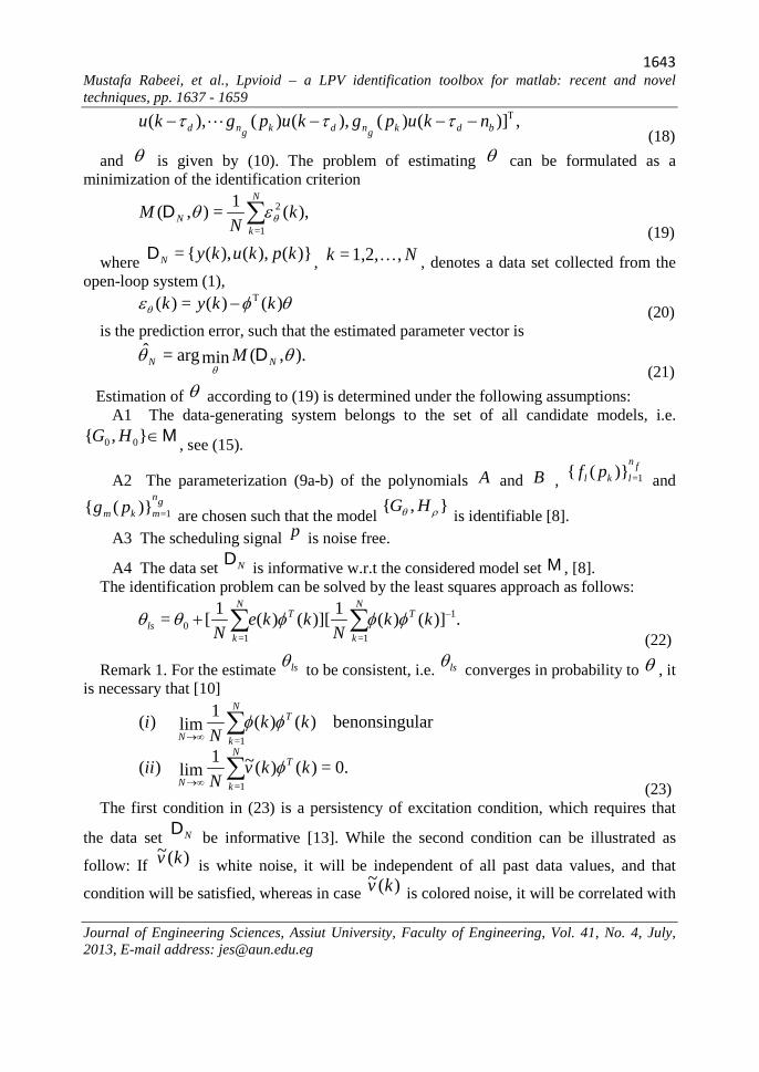
using the Model Output option in the evaluation board and the BFR (47) is found to be 82.388% , see Fig. 5. The RIV method gives a good estimates of both plant and noise model parameters, relative to a SNR of 15 dB, as indicated in table 1. Other options can be applied to perform more evaluation of the estimated model, see section 4.



Fig. 5. LPVIOID open-loop model output

Table 1. Open-loop identification

estimated parameters of the A polynomial method 1,1a 1,2a 1,3a 2,1a 2,2a 2,3a EXACT 1 -0.5 -0.1 0.5 -0.7 -0.1

RIV 0.9939 -0.5070 -0.0295 0.5088 -0.7850 0.0282 estimated parameters of the B polynomial

method 1,1b 1,2b 1,3b 2,1b 2,2b 2,3b EXACT 0.5 -0.4 0.01 0.2 -0.3 -0.02

RIV 0.5007 -0.4060 0.0167 0.1976 -0.3107 0.0087 the estimated HA and HB polynomials’ parameters

method ,1Ha ,1Hb EXACT 0.3 0.5

RIV 0.3194 0.4926



5. 3. Closed-loop identification for stable plants For closed-loop identification, see section 2.3, the plant (1) with the coefficients (48-49)

is simulated with a stabilizing controller

1

1

0.8510.51=)( −

−

−+

qqqK (53)

and the scheduling variable as given in (50) with 1=η , such that the open-loop and closed-loop systems be stable in the whole scheduling range. In the simulation, the reference signals )(1 kr and )(2 kr are both taken as white noise with a uniform distribution 1,1)(−U and a number of data sample 4000=N , )(ke is taken as a white noise disturbance with uniform distribution )(0, 2µN with 0.0075=µ to produce a SNR = 15 dB and the noise model (52) is considered. The RIV identification method in LPVIOID is applied, with 1=1,=1,=2,= aHdba nnnn and 1=bHn . Estimated model parameters are listed in table 1 and the simulated model output is compared in Fig. 6 with the true system output.

Fig. 6. LPVIOID closed-loop model output As shown in table 2 and Fig. 6, the RIV method gives good estimation of the plant and

the noise-model parameters with a 78.65.=BFR



Table 2. Closed-loop identification

the estimated A polynomial parameters Method

1,1a 1,2a 1,3a 2,1a 2,2a 2,3a EXACT 1 -0.5 -0.1 0.5 -0.7 -0.1 RIV 0.9992 -0.4441 -0.1887 0.4971 -0.6503 -0.1760

the estimated B polynomial’s parameters Method

1,1b 1,2b 1,3b 2,1b 2,2b 2,3b EXACT 0.5 -0.4 0.01 0.2 -0.3 -0.02 RIV 0.4975 -0.3943 0.0068 0.1997 -0.2891 -0.0352

the estimated HA and HB polynomials’ parameters Method

,1Ha ,1Hb EXACT 0.3 0.5 RIV 0.3767 0.5651

5. 4. Closed-loop identification with unstable plant

Finally, the same plant used above is made unstable, by putting 1.7=η in the scheduling variable expression (50). To stabilize the closed loop system, see Fig. 3, for that new range of scheduling variable we use the following controller

.0.20.11

0.50.1=)( 11

11

−−

−−

++−

qqqqqK (54)

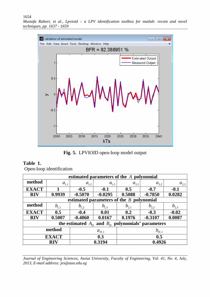
Next the closed-loop system is simulated using )(kr taken as a white noise with a uniform distribution 1,1)(−U , a number of data samples 4000=N and an additive white noise disturbance )(0,)( 2µN∈ke with 0.0025=µ , to produce a dBSNR 15= . The noise model is taken as 1=H , i.e. OE type. Estimated parameters using the LS, IV, and iterative-LS methods, explained in section 3, respectively, are shown in table 3. Using the option Compare under the menu Model, the three estimated models’ outputs were plotted in a single figure as shown in Fig. 7 and the BFR of each model is also calculated. From table 3 and Fig. 7 it is found that LS provides biased estimate, iterative LS gives a little better estimate, while, IV gives the best estimate, 81.226%=BFR .



Fig. 7. LPVIOID closed-loop model output

Table 3. Unstable plant identification

the estimated A polynomial parameters

method 1,1a 1,2a 1,3a 2,1a 2,2a 2,3a

EXACT 1 -0.5 -0.1 .5 -0.7 -0.1 LS 0.7919 -0.2102 -0.1691 0.3710 -0.5207 -0.1183 IV 0.9825 -0.4715 -0.1435 0.4799 -0.7226 -0.0827

iterative-LS 0.7923 -0.2127 -0.1673 0.3706 -0.5230 -0.1164

the estimated B polynomial parameters method

1,1b 1,2b 1,3b 2,1b 2,2b 2,3b

EXACT .5 -0.4 0.01 0.2 -0.3 -.02 LS 0.4959 -0.3884 0.0041 0.1390 -0.2051 -0.0531 IV 0.4959 -0.3863 0.0035 0.1990 -0.3138 -0.0122

iterative-LS 0.4958 -0.3890 0.0044 0.1390 -0.2045 -0.0536



6. Conclusions and future work This paper has presented the LPVIOID, a system identification toolbox for MATLAB to

identify LPV-IO models. The toolbox comprises the more recent identification methodologies and supported with a user friendly graphical user interface (GUI). Furthermore the toolbox supports both open-/closed-loop identification and includes many options for model evaluation in time and frequency domains. A novel technique for the identification of unstable LPV-IO plants in closed-loop has been introduced and embedded in the LPVIOID. The current version of LPVIOID deals with the SISO LPV models only, an extension to the MIMO case is a straightforward future work.

7. References [1] H. Abbas, M. Ali, and H. Werner. Linear Recurrent Neural Network for open- and closed-

loop consistent identification of LPV models. In IEEE Conference on Decision and Control (CDC), pages 6851–6856, Atlanta, Georgia, USA, 2010.

[2] A. Ali, M. Ali, and H. Werner. Indirect closed-loop identification of input-output LPV models: A pre-filtering approach. In Proc. of the 18th IFAC World Congress, pages 4186–4191, Milan, Italy, 2011.

[3] P. Apkarian and P. Gahinet A Convex Characterization of Gain-Scheduled H ∞ Controllers IEEE Trans. Automatic Control, vol. 40, no. 5, pp. 853-864, 1995

[4] B. Bamieh and L. Giarré. Identification of linear parameter varying models. International Journal of Robust and Nonlinear Control, 12(9):841–853, 2002.

[5] M. Butcher, A. Karimi, and R. Longchamp. On the consistency of certain identification methods for linear parameter varying systems. In Proc. of the 17th IFAC World Congress, pages 4018–4023, Seoul, Korea, 2008.

[6] W. Gilbert, D. Henrion, J. Bernussou, and D. Boyer. Polynomial LPV synthesis applied to turbofan engine. IFAC Control Engineering Practice, 18(9):1077–1083, 2010. , Engineering Department, 2002.

[7] A. Kominek, H. Werner, M. Garwon, and M. Schultalbers. Control of Linear Parameter Varying Systems with Applications, chapter Identification of Low-Complexity LPV Input-Output Models for Control of a Turbocharged Combustion Engine. Springer US, 2012.

[8] V. Laurain, M. Gilson, R. Tóth, and H. Garnier. Refined instrumental variable methods for identification of LPV box-jenkins models. Automatica, 46(6):959–967, 2010.

[9] L. Ljung, System Identification Toolbox, for use with Matlab. The Mathworks Inc., 2006. [10] L. Ljung. System Identification, Theory for the User. Prentice-Hall Inc. USA, 2nd edition

edition, 1999. [11] C.W. Scherer. Robust generalized H2 control for uncertain and LPV systems with general

scalings. In Proc. of the 47th IEEE Conference on Decision and Control, Kobe, Japan, 4(0):3970–3975, 1996.

[12] T. Söderström and P. Stoica. Instrumental Variable Methods for System Identification. Springer-Verlag, 1983.

[13] R. Tóth, P. Heuberger, and P. Van den Hof. Control of Linear Parameter Varying Systems with Applications, chapter Prediction-Error Identification of LPV Systems: Present and Beyond. Springer US, 2012.



[14] R. Tóth, V. Laurain, M. Gilson, and H. Garnier. On the closed loop identification of LPV models using instrumental variables. In Proc. of the 18th IFAC World Congress, pages 7773–7778, Milan, Italy, 2011.

[15] V. Verdult. A Kernel Method for Subspace Identification of Multivariable Bilinear Systems. In Ph.D thesis, Univesity of Twente, 2002.

[16] Herbert Werner: Robust control design with Matlab: D.-W. Gu, P.Hr. Petkov, M.M. Konstantinov; Springer-Verlag London Limited, ISBN: 1-85233-983-7. Automatica 42(9): 1619-1620 (2006).

باستخدام الماتالب تضم طرق حديثه ةبرمجيه تفاعليه للنمذج المتغيرة ذات المعامالت الخطية ة لألنظمالمعملية ةو مبتكره في النمذج

الملخص العربي ةإلجراء النمذج (MATLAB) ) باستخدام برنامج LPVIOIDيقدم البحث حزمه برمجيه تفاعليه (

الطرق األكثر ةالحزم ) . تضم هذهLPV (ة ذات المعامالت المتغيرة الخطية للنظم الديناميكيةالمعملي النظم الغير ةلي تقنيه مبتكره تصلح لنمذجإ ة، باإلضافة النظم ذات المعامالت المتغيرة في مجال نمذجةحداث ة. تتيح هذه البرمجية باستخدام قياسات مجمعه من نظم تحكم مغلقه الحلق )unstable systems( متزنه

مجمعه سواء قياسات ) باستخدامdiscrete-time (ة المتقطعة لألنظمةجراء عمليه النمذجإ ةمكانيإ ةالمقترح علي توافر العديد من الطرق (األدوات) لتقييم النموذج ة، عالوة الحلقةو مفتوحأ ةمن انظمه مغلقه الحلق

. توضيحيهةمثلأ عده أيضا يشمل البحث الناتج و كل ذلك بطريقه عمليه.

LPVIOID- A LPV IDENTIFICATION TOOLBOX FOR MATLAB: RECENT ... · In this paper a system identification toolbox for MATLAB is ... Lpvioid a LPV identification toolbox for ... Lpvioid

Documents