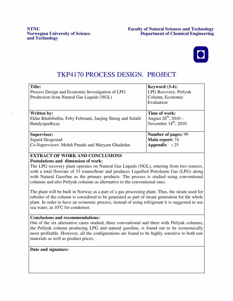
NTNU Faculty of Natural Sciences and Technology Norwegian University of Science Department of Chemical Engineering and Technology TKP4170 PROCESS DESIGN. PROJECT Title: Process Design and Economic Investigation of LPG Production from Natural Gas Liquids (NGL) Keyword (3-4): LPG Recovery, Petlyuk Column, Economic Evaluation Written by: Eldar Khabibullin, Feby Febrianti, Juejing Sheng and Sulalit Bandyopadhyay Time of work: August 26 th , 2010 – November 18 th , 2010 Supervisor: Sigurd Skogestad Co-Supervisors: Mehdi Panahi and Maryam Ghadrdan Number of pages: 99 Main report: 74 Appendix : 25 EXTRACT OF WORK AND CONCLUSIONS Postulations and dimension of work: The LPG recovery plant operates on Natural Gas Liquids (NGL), entering from two sources, with a total flowrate of 33 tonnes/hour and produces Liquified Petroleum Gas (LPG) along with Natural Gasoline as the primary products. The process is studied using conventional columns and also Petlyuk columns as alternative to the conventional ones. The plant will be built in Norway as a part of a gas processing plant. Thus, the steam used for reboiler of the column is considered to be generated as part of steam generation for the whole plant. In order to have an economic process, instead of using refrigerant it is suggested to use sea water, at 10 o C for condenser. Conclusions and recommendations: Out of the six alternative cases studied, three conventional and three with Petlyuk columns, the Petlyuk column producing LPG and natural gasoline, is found out to be economically most profitable. However, all the configurations are found to be highly sensitive to both raw materials as well as product prices. Date and signature: -

Welcome message from author
This document is posted to help you gain knowledge. Please leave a comment to let me know what you think about it! Share it to your friends and learn new things together.
Transcript
NTNU Faculty of Natural Sciences and Technology Norwegian University of Science Department of Chemical Engineering and Technology
TKP4170 PROCESS DESIGN. PROJECT
Title: Process Design and Economic Investigation of LPG Production from Natural Gas Liquids (NGL)
Keyword (3-4): LPG Recovery, Petlyuk Column, Economic Evaluation
Written by: Eldar Khabibullin, Feby Febrianti, Juejing Sheng and Sulalit Bandyopadhyay
Time of work: August 26th, 2010 – November 18th, 2010
Supervisor: Sigurd Skogestad Co-Supervisors: Mehdi Panahi and Maryam Ghadrdan
Number of pages: 99 Main report: 74 Appendix : 25
EXTRACT OF WORK AND CONCLUSIONS Postulations and dimension of work: The LPG recovery plant operates on Natural Gas Liquids (NGL), entering from two sources, with a total flowrate of 33 tonnes/hour and produces Liquified Petroleum Gas (LPG) along with Natural Gasoline as the primary products. The process is studied using conventional columns and also Petlyuk columns as alternative to the conventional ones.
The plant will be built in Norway as a part of a gas processing plant. Thus, the steam used for reboiler of the column is considered to be generated as part of steam generation for the whole plant. In order to have an economic process, instead of using refrigerant it is suggested to use sea water, at 10oC for condenser.
Conclusions and recommendations: Out of the six alternative cases studied, three conventional and three with Petlyuk columns, the Petlyuk column producing LPG and natural gasoline, is found out to be economically most profitable. However, all the configurations are found to be highly sensitive to both raw materials as well as product prices.
Date and signature:
-
ii
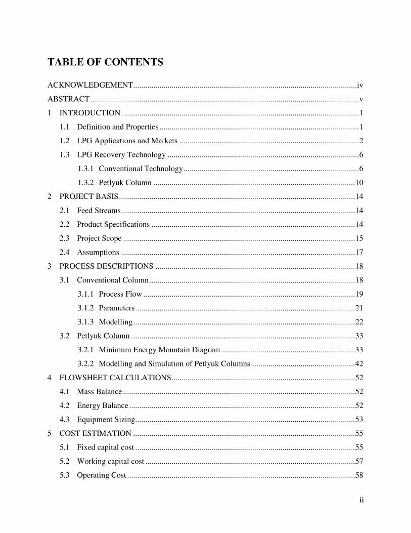
TABLE OF CONTENTS
ACKNOWLEDGEMENT ...............................................................................................................iv
ABSTRACT ..................................................................................................................................... v
1 INTRODUCTION ...................................................................................................................... 1
1.1 Definition and Properties ................................................................................................... 1
1.2 LPG Applications and Markets ......................................................................................... 2
1.3 LPG Recovery Technology ............................................................................................... 6
1.3.1 Conventional Technology ....................................................................................... 6
1.3.2 Petlyuk Column .................................................................................................... 10
2 PROJECT BASIS ..................................................................................................................... 14
2.1 Feed Streams .................................................................................................................... 14
2.2 Product Specifications ..................................................................................................... 14
2.3 Project Scope ................................................................................................................... 15
2.4 Assumptions .................................................................................................................... 17
3 PROCESS DESCRIPTIONS ................................................................................................... 18
3.1 Conventional Column ...................................................................................................... 18
3.1.1 Process Flow ......................................................................................................... 19
3.1.2 Parameters ............................................................................................................. 21
3.1.3 Modelling .............................................................................................................. 22
3.2 Petlyuk Column ............................................................................................................... 33
3.2.1 Minimum Energy Mountain Diagram .................................................................. 33
3.2.2 Modelling and Simulation of Petlyuk Columns ................................................... 42
4 FLOWSHEET CALCULATIONS ........................................................................................... 52
4.1 Mass Balance ................................................................................................................... 52
4.2 Energy Balance ................................................................................................................ 52
4.3 Equipment Sizing ............................................................................................................. 53
5 COST ESTIMATION .............................................................................................................. 55
5.1 Fixed capital cost ............................................................................................................. 55
5.2 Working capital cost ........................................................................................................ 57
5.3 Operating Cost ................................................................................................................. 58

iii
6 INVESTMENT ANALYSIS .................................................................................................... 64
6.1 Internal Rate of Return .................................................................................................... 64
6.2 Net Present Value ............................................................................................................ 65
6.3 Pay-back Period ............................................................................................................... 65
6.4 Sensitivity Analysis ......................................................................................................... 66
7 DISCUSSION .......................................................................................................................... 68
8 CONCLUSIONS AND RECOMMENDATIONS ................................................................... 69
LIST OF SYMBOLS ...................................................................................................................... 70
REFERENCES ............................................................................................................................... 73
APPENDICES ................................................................................................................................ 75
Appendix A - Computational Procedure for Vmin diagram....................................................... 75
Appendix B – Equipment Sizing .............................................................................................. 81
Appendix C - Petlyuk Column Calculations ............................................................................ 87
Appendix D - Steam Calculations for Petlyuk Column ........................................................... 93
Appendix E - Capital Cost Estimation ..................................................................................... 94
Appendix F – Cash Flows for Different Alternatives .............................................................. 99
iv
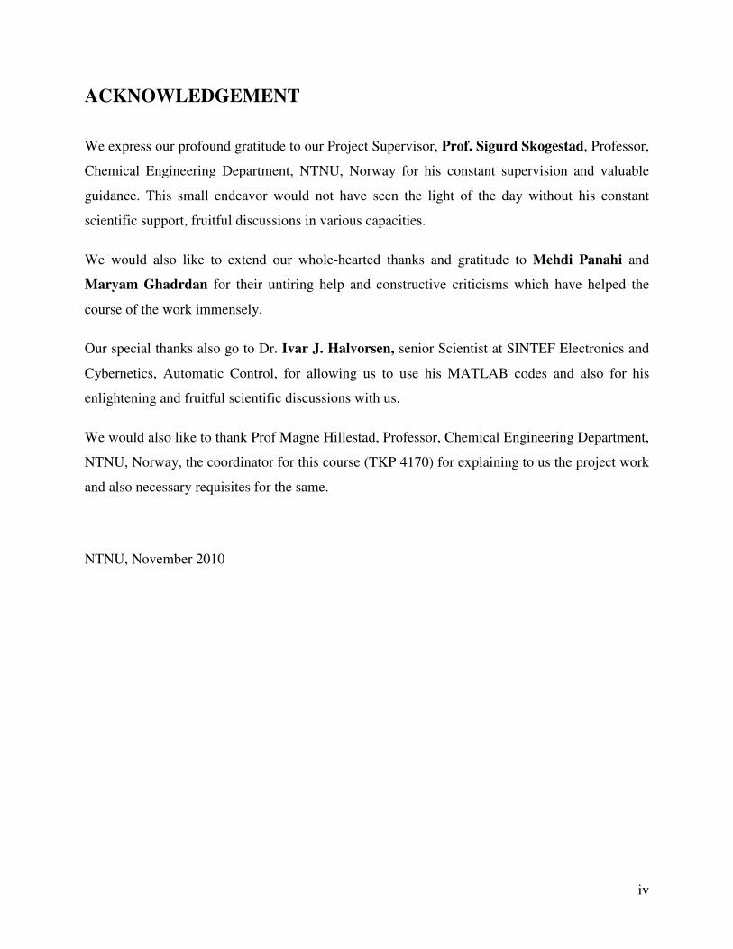
ACKNOWLEDGEMENT
We express our profound gratitude to our Project Supervisor, Prof. Sigurd Skogestad, Professor,
Chemical Engineering Department, NTNU, Norway for his constant supervision and valuable
guidance. This small endeavor would not have seen the light of the day without his constant
scientific support, fruitful discussions in various capacities.
We would also like to extend our whole-hearted thanks and gratitude to Mehdi Panahi and
Maryam Ghadrdan for their untiring help and constructive criticisms which have helped the
course of the work immensely.
Our special thanks also go to Dr. Ivar J. Halvorsen, senior Scientist at SINTEF Electronics and
Cybernetics, Automatic Control, for allowing us to use his MATLAB codes and also for his
enlightening and fruitful scientific discussions with us.
We would also like to thank Prof Magne Hillestad, Professor, Chemical Engineering Department,
NTNU, Norway, the coordinator for this course (TKP 4170) for explaining to us the project work
and also necessary requisites for the same.
NTNU, November 2010

v
ABSTRACT
Liquefied Petroleum Gas (LPG) is used as a potential fuel in several parts of the world. The price
of LPG has been steadily increasing over the last few years as demand for the product has
increased and oil prices have shifted upwards. It is generally synthesized from crude oil (40%) or
from natural gas (60%). This project mainly focuses on design and simulation of an LPG plant,
which processes feed from natural gas wells to produce LPG along with, natural gasoline (C5+)
having a higher value as separate product. The same is carried out using two alternatives, the
conventional approach and the use of Petlyuk columns, as a means to heat-integrate and reduce
operating as well as investment costs.
Six cases are studied with various final products, decided based on market studies and different
column configurations, analyzed on an economic basis. There are two feeds to the plant, one from
the Natural gas (NG) wells, containing around 79% of C5+ and the other from dehydration units
of NG processing plants, containing 52% C5+, with a total flowrate of 34 tonnes/hr. UNISIM
simulations have been done for all the conventional cases in order to setup the process flow
sheets and size the various equipments, while short cut calculations have been done for the
Petlyuk columns to arrive at comparable states with the conventional.
Economic analysis, with internal rate of return (IRR) and Net present worth (NPW) as the
economic parameters have been carried out for all the six cases. The Petlyuk configurations
appear more profitable as compared to the conventional cases, with the Petlyuk configuration
producing LPG and natural gasoline (C5+), seemingly the best. However, sensitivity analysis
shows that the project is highly sensitive to change in raw material prices and product prices,
hence, this could turn out to be a risky project for a new investor, while, it would be not so for an
already established big industrial company.
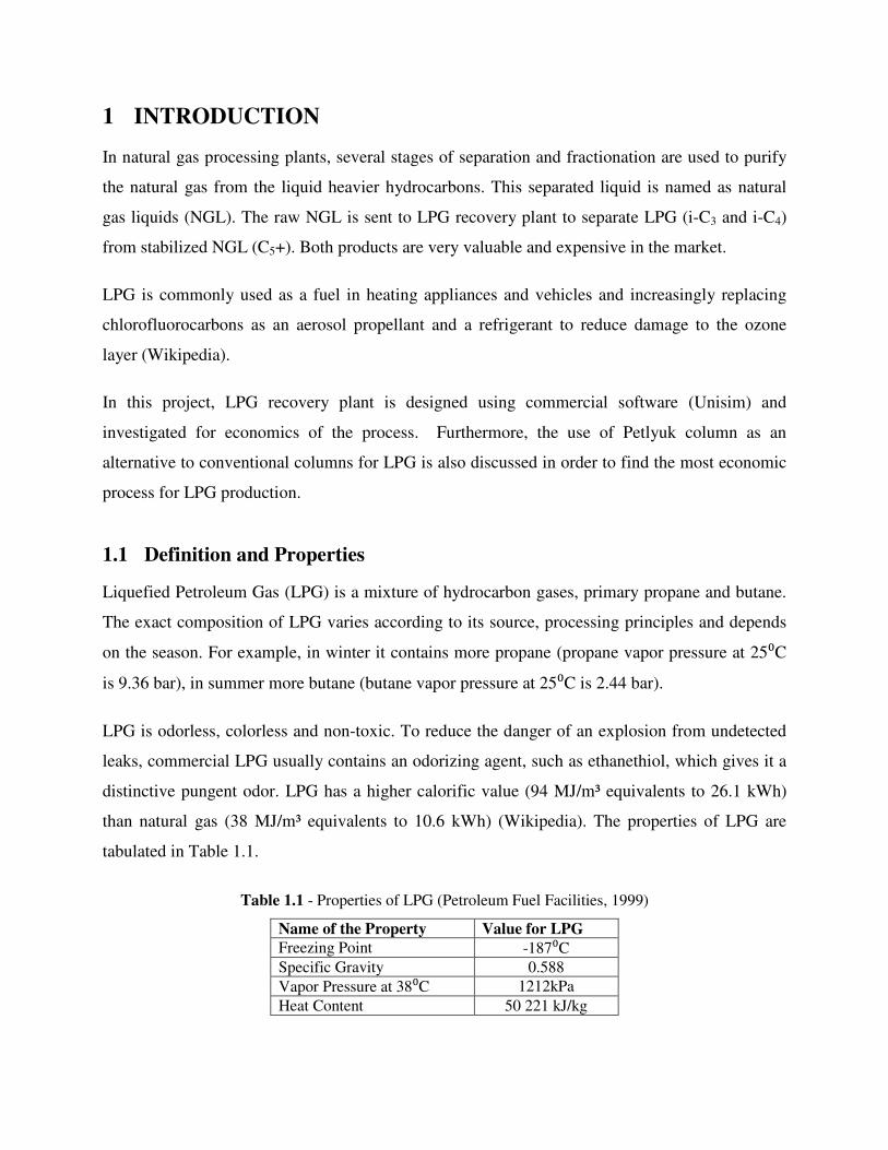
1 INTRODUCTION
In natural gas processing plants, several stages of separation and fractionation are used to purify
the natural gas from the liquid heavier hydrocarbons. This separated liquid is named as natural
gas liquids (NGL). The raw NGL is sent to LPG recovery plant to separate LPG (i-C3 and i-C4)
from stabilized NGL (C5+). Both products are very valuable and expensive in the market.
LPG is commonly used as a fuel in heating appliances and vehicles and increasingly replacing
chlorofluorocarbons as an aerosol propellant and a refrigerant to reduce damage to the ozone
layer (Wikipedia).
In this project, LPG recovery plant is designed using commercial software (Unisim) and
investigated for economics of the process. Furthermore, the use of Petlyuk column as an
alternative to conventional columns for LPG is also discussed in order to find the most economic
process for LPG production.
1.1 Definition and Properties
Liquefied Petroleum Gas (LPG) is a mixture of hydrocarbon gases, primary propane and butane.
The exact composition of LPG varies according to its source, processing principles and depends
on the season. For example, in winter it contains more propane (propane vapor pressure at 25⁰C
is 9.36 bar), in summer more butane (butane vapor pressure at 25⁰C is 2.44 bar).
LPG is odorless, colorless and non-toxic. To reduce the danger of an explosion from undetected
leaks, commercial LPG usually contains an odorizing agent, such as ethanethiol, which gives it a
distinctive pungent odor. LPG has a higher calorific value (94 MJ/m³ equivalents to 26.1 kWh)
than natural gas (38 MJ/m³ equivalents to 10.6 kWh) (Wikipedia). The properties of LPG are
tabulated in Table 1.1.
Table 1.1 - Properties of LPG (Petroleum Fuel Facilities, 1999)
Name of the Property Value for LPG Freezing Point -187⁰C
Specific Gravity 0.588
Vapor Pressure at 38⁰C 1212kPa
Heat Content 50 221 kJ/kg

2
1.2 LPG Applications and Markets
Application of LPG varies from food to transport industry. Its consumption depends on the local
market conditions. LPG is widely used in the Food Industry like hotels, restaurants, bakeries,
canteens, resorts etc. Low sulphur content and controllable temperature makes LPG the most
preferred fuel in the food industry.
Glass & Ceramic
The manufacture of glass / ceramic products is complicated by numerous chemical reactions
which occur during the process. The use of a clean fuel like LPG enhances the product quality
thereby reducing technical problems related to the manufacturing activity. LPG being a gaseous
fuel gets easily regulated and complements the heating process.
Building Industry
LPG being a premium gaseous fuel makes it ideal for usage in the Cement manufacturing
process. The ease in regulation and soft quality of the LPG flame and low sulphur content are the
key advantages both with regard to cement quality and kiln operability.
Metal Industry
The metal industry is indeed one of the most important consumers of energy. LPG being a far
superior fuel as compared to the other heavy fuels helps improve the cost of operation and strikes
an economic balance between fuel price and quality of the end product. The application is
basically for cutting, heating and melting. Both ferrous and non-ferrous metals are frequently cast
into shapes by melting and injection or pouring into suitable patterns and moulds. LPG in this
case is an ideal fuel for meeting the requirement of temperature regulation and desired quality.
Farming Industry
LPG is the ideal fuel for production of food by agriculture and animal husbandry. Drying of crops
and other farm products requires clean and sulphur free fuel for drying activity to avoid any
transfer of bad taste or smell to the dried crops.

3
Aerosol Industry
An aerosol formulation is a blend of an active ingredient with propellant,emulsifiers, perfumes,
etc. LPG, being environment friendly, has replaced the ozone depleting CFC gases which were
earlier used by the aerosol Industry.
Automotive Industry
Automotive LPG is a clean fuel with high octane, aptly suited for vehicles both in terms of
emissions and cost of the fuel. The main advantage of using automotive LPG: it is free of lead,
very low in sulphur, metals, aromatics and other contaminants. Unlike natural gas, LPG is not a
Green House Gas. The following table lists the preferred LPG composition in Europe.
Table 1.2 - LPG Composition (% by Volume) as Automotive Fuel in Europe (West Virginia University)
Country Propane Butane Austria 50 50
Belgium 50 50
Denmark 50 50
France 35 65
Greece 20 80
Ireland 100 -
Spain 30 70
Sweden 95 5
United Kingdom 100 -
Germany 90 10
Cogeneration using LPG
LPG is an ideal fuel for electricity & heat / electricity and comfort cooling. This finds varied
applications in industries requiring power and steam, power and hot air. LPG is ideally suited for
shopping malls, offices requiring power and air conditioning.
LPG has lower calorific value then petrol, so it provides less miles per gallon, however in
European countries LPG tax levels are much lower than both diesel and unleaded so it is still a far
more cost effective way to run your car. The tax break is due to evidence that suggests that LPG
is better for the environment than the mainstream fuels.
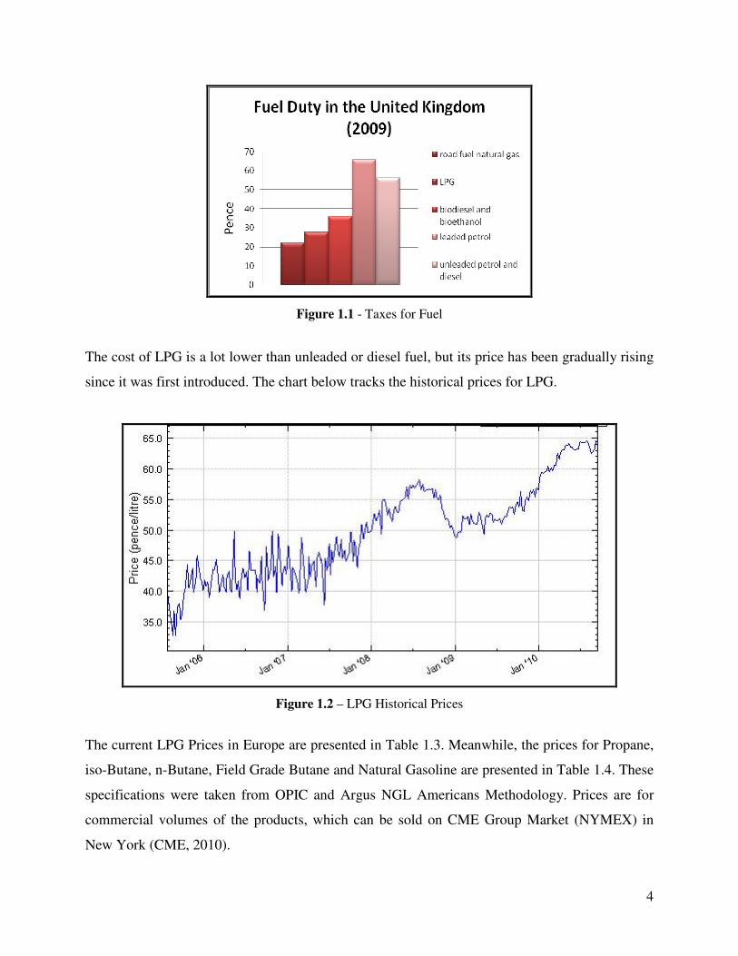
4
Figure 1.1 - Taxes for Fuel
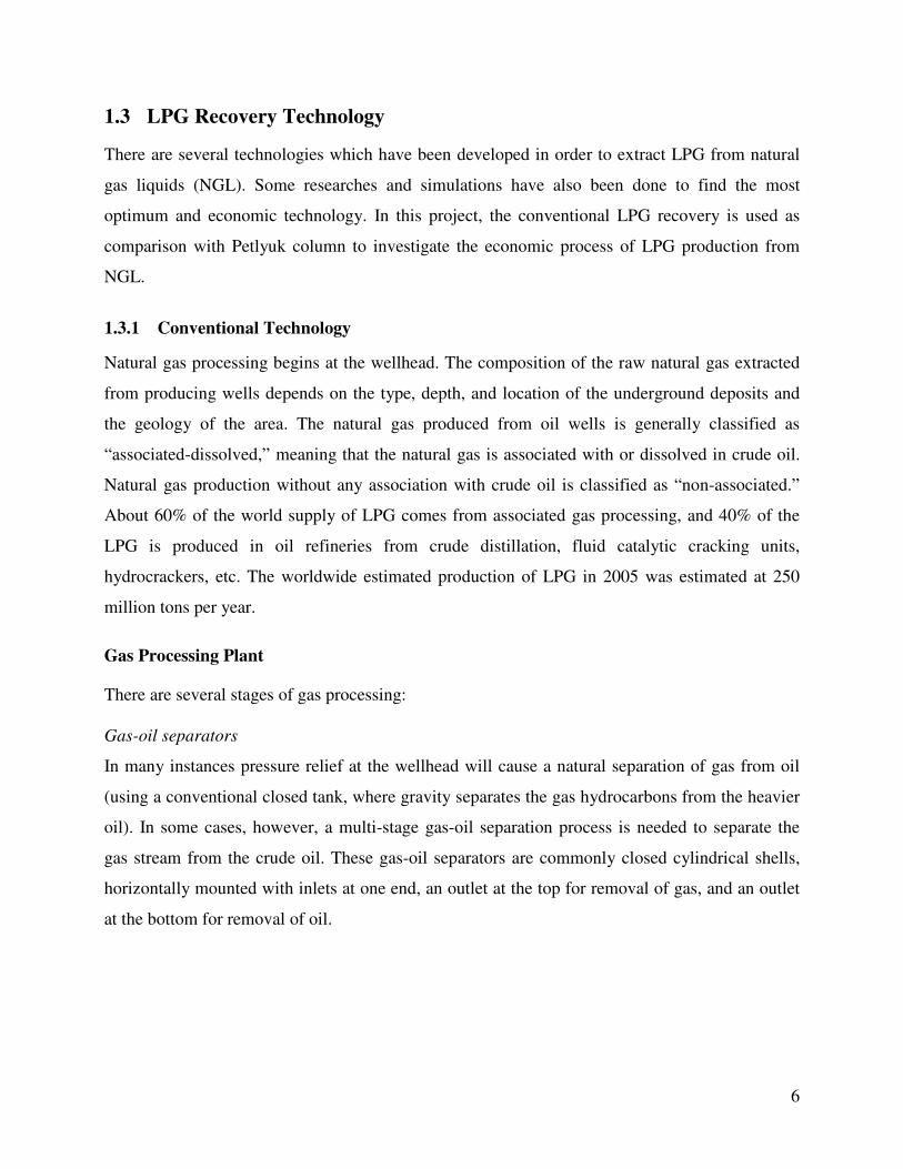
The cost of LPG is a lot lower than unleaded or diesel fuel, but its price has been gradually rising
since it was first introduced. The chart below tracks the historical prices for LPG.
Figure 1.2 – LPG Historical Prices
The current LPG Prices in Europe are presented in Table 1.3. Meanwhile, the prices for Propane,
iso-Butane, n-Butane, Field Grade Butane and Natural Gasoline are presented in Table 1.4. These
specifications were taken from OPIC and Argus NGL Americans Methodology. Prices are for
commercial volumes of the products, which can be sold on CME Group Market (NYMEX) in
New York (CME, 2010).

5
Table 1.3 – LPG Prices in Europe (www.energy.eu)
Table 1.4 – LPG Specifications and Prices
Product Specification Price ($/gallon) Price ($/kg)
Propane 90% propane minimum, 5% propylene maximum, 0.507 relative density and 90,830 btu/gal
1.17594 0.62447
Iso-Butane 96% iso-butane minimum, 4% normal butane maximum, 3% propane maximum, 0.563 relative density and 98,950 btu/gal
1.60083 0.7761
n-Butane 94% normal butane minimum, 6% iso-butane maximum, 0.35% propane maximum, 1.5% pentanes and heavier maximum, 0.35% olefins maximum, 0.584 relative density and 102,916 btu/gal
1.54661 0.75447
Field Grade Butane
Mix of n-Butane and Iso-Butane (35% iC4+ 65% nC4)
1.4383 0.76213
Natural Gasoline C5+, 0.664 relative density and 115,021 btu/gal
1.90315 1.08716
6
1.3 LPG Recovery Technology
There are several technologies which have been developed in order to extract LPG from natural
gas liquids (NGL). Some researches and simulations have also been done to find the most
optimum and economic technology. In this project, the conventional LPG recovery is used as
comparison with Petlyuk column to investigate the economic process of LPG production from
NGL.
1.3.1 Conventional Technology
Natural gas processing begins at the wellhead. The composition of the raw natural gas extracted
from producing wells depends on the type, depth, and location of the underground deposits and
the geology of the area. The natural gas produced from oil wells is generally classified as
“associated-dissolved,” meaning that the natural gas is associated with or dissolved in crude oil.
Natural gas production without any association with crude oil is classified as “non-associated.”
About 60% of the world supply of LPG comes from associated gas processing, and 40% of the
LPG is produced in oil refineries from crude distillation, fluid catalytic cracking units,
hydrocrackers, etc. The worldwide estimated production of LPG in 2005 was estimated at 250
million tons per year.
Gas Processing Plant
There are several stages of gas processing:
Gas-oil separators
In many instances pressure relief at the wellhead will cause a natural separation of gas from oil
(using a conventional closed tank, where gravity separates the gas hydrocarbons from the heavier
oil). In some cases, however, a multi-stage gas-oil separation process is needed to separate the
gas stream from the crude oil. These gas-oil separators are commonly closed cylindrical shells,
horizontally mounted with inlets at one end, an outlet at the top for removal of gas, and an outlet
at the bottom for removal of oil.
7
Condensate separator
Condensates are most often removed from the gas stream at the wellhead through the use of
mechanical separators. In most instances, the gas flow into the separator comes directly from the
wellhead, since the gas-oil separation process is not needed.
Dehydration
A dehydration process is needed to eliminate water which may cause the formation of hydrates.
Hydrates form when a gas or liquid containing free water experiences specific
temperature/pressure conditions. Dehydration is the removal of this water from the produced
natural gas and is accomplished through several methods. Among these is the use of ethylene
glycol (glycol injection) system as an absorption mechanism to remove water and other solids
from the gas stream. Alternatively, adsorption dehydration may be used, utilizing dry-bed
dehydrators towers, which contain desiccants such as silica gel and activated alumina, to perform
the extraction.
Contaminant removal
Removal of contaminants includes the elimination of hydrogen sulphide, carbon dioxide, water
vapor, helium, and oxygen. The most commonly used technique is to first direct the flow though
a tower containing an amine solution. Amines absorb sulphur compounds from natural gas and
can be reused repeatedly. After desulphurization, the gas flow is directed to the next section,
which contains a series of filter tubes. As the velocity of the stream reduces in the unit, primary
separation of remaining contaminants occurs due to gravity.
Methane separation
Cryogenic processing and absorption methods are some of the ways to separate methane from
natural gas liquids (NGLs). The cryogenic method is better at extraction of the lighter liquids,
such as ethane, than is the alternative absorption method. Essentially, cryogenic processing
consists of lowering the temperature of the gas stream to around -120 degrees Fahrenheit. While
there are several ways to perform this function, the turbo expander process is most effective,
using external refrigerants to chill the gas stream. The quick drop in temperature that the
expander is capable of producing, condenses the hydrocarbons in the gas stream, but maintains
methane in its gaseous form.
8
The absorption method, on the other hand, uses a “lean” absorbing oil to separate the methane
from the NGLs. While the gas stream is passed through an absorption tower, the absorption oil
soaks up a large amount of the NGLs. The “enriched” absorption oil, now containing NGLs, exits
the tower at the bottom. The enriched oil is fed into distillers where the blend is heated to above
the boiling point of the NGLs, while the oil remains fluid. The oil is recycled while the NGLs are
cooled and directed to a fractionator tower. Another absorption method that is often used is the
refrigerated absorption method where the lean oil is chilled rather than heated, a feature that
enhances recovery rates somewhat (Tobin et al., 2006).
Fractionation
The stripper bottom product from the LPG extraction plant consists of propane, butane and
natural gasoline with some associated ethane and lighter components. This is the feed to the LPG
fractionation plant where it is separated into a gas product, propane, butane and NGL.
LPG Fractionation Plant
Most commonly used LPG fractionation system is described in Figure 1.3.
Figure 1.3 – LPG Fractionation System

9
Deethanizer
As can be seen from the Figure 1.3, the stripper bottoms from the extraction plant enter
deethanizer column V-101 near the top. The overhead vapor is partially condensed in deethanizer
condenser E-101 by heat exchange with medium-level propane at -6.67 °C. Condensed overhead
product in overhead reflux drum V-104 is pumped back to the deethanizer by reflux pump. The
non-condensed vapor, mainly ethane, leaves the plant to fuel the gas system. Heat is supplied to
the column by forced circulation reboiler E-104. The deethanizer column operates at
approximately 26.9 bar. Approximately 98% of the propane in the deethanizer feed is recovered
in the bottom product. The residual ethane concentration is reduced to approximately 0.8 mole %
in the bottom product. The bottom product from deethanizer drains into depropanizer column V-
102.
Depropanizer
Deethanizer bottoms are expanded from 26.9 bar to 20 bar and enter depropanizer V-102 as
mixed-phase feed. The depropanizer fractionates the feed into a propane-rich product and a
bottom product comprised of butane and natural gasoline. Tower V-102 overhead vapor is totally
condensed in the depropanizer condenser E-102 by cooling water. Condensate is collected in
depropanizer column reflux drum V-105. A part of the condensed overhead product is sent back
to the column as reflux via pump P-103 while the remaining part is withdrawn as a liquid propane
product. Column V-102 reboiler heat is supplied by direct-fired heater H-101. Reboiler
circulation is aided by reboiler circulation pump P-104. The bottom product is sent to
debutanizer.
Debutanizer
The depropanizer bottoms are expanded from approximately 20 bar to 7.6 bar and then enter the
debutanizer column as a mixed-phase feed. The column feed is fractionated into a butane-rich
overhead product and natural gasoline bottoms. The columns overhead are totally condensed in
the debutanizer condenser E-103 by heat exchange with cooling water, and condensate is
collected in reflux drum V-106. The debutanizer reflux and product pump P-105 serve the dual
purpose of supplying reflux to the column and allowing withdrawal of column overhead product
butane from the reflux drum. The column reboil heat is supplied by a direct-fired debutanizer
reboiler H-102, and boiler circulation is aided by debutanizer reboiler circulating pump P-106.
10
The bottom product leaving the column is cooled in product cooler E-105. A part of the gasoline
product is recycled to the LPG extraction unit and serves as lean oil for the absorber column
(Parkash, 2003).
Product Treatment Plant
Propane and butane products from the fractionation plant contain impurities in the form of
sulphur compounds and residual water that must be removed to meet product specifications. The
impurities are removed by absorption on molecular sieves. Each product is treated in a twin
fixed-bed molecular sieve unit. Regeneration is done by sour gas from the stripper overhead
followed by vaporized LPG product. Operating conditions are listed in Table 1.5 and impurities
to be removed are listed in Table 1.6.
Table 1.5 – Molecular Sieve Product Treating Process Operating Conditions
Operating variable Units Propane Butane Pressure Bar 22.4 10.7
Temperature C0 43.3 43.3
Phase Liquid Liquid
Table 1.6 – Typical Contaminant Level in Untreated LPG
Contaminants Units Propane Butane H2O wt ppm 10 Trace
H2S wt ppm 100 Trace
COS wt ppm 34 Trace
C3SH wt ppm 100 40
C2H5SH wt ppm Trace 220
1.3.2 Petlyuk Column
Distillation plays an important role in splitting raw product streams into more useful product
streams with specified compositions. It is particularly well suited for high purity separations since
any degree of separation can be obtained with a fixed energy consumption by increasing the
number of equilibrium stages. However, industrial distillation processes are commonly known to
be highly energy-demanding operations. According to Ognisty (1995), the energy inputs to
distillation columns account for roughly 3% of the total energy consumption in the U.S
(Christiansen et al., 1997). Thus, it becomes an obvious challenge to devise newer technologies to

11
facilitate energy efficient separation arrangements. This study aims at using Petlyuk columns as
an alternative to conventional configuration.
In order to increase the process efficiency of such distillation processes, the following two
alternatives have been proposed both in the literature and by industrial practitioners. These
include:
a. Integration of Conventional Distillation Arrangements - Includes sequential arrangement of
distillation columns with energy integration between the columns or other parts of the plant.
b. Design of new configurations - Includes Dividing Wall Column; which consists of an
ordinary column shell with the feed and side stream product draw divided by a vertical wall
through a set of trays, first proposed by Wright (1949). The same configuration is usually
denoted as a Petlyuk column after Petlyuk et al (1965) who studied the scheme
theoretically. The fully thermally coupled column (Triantafyllou and Smith 1992) is also a
modification of the Dividing Wall Column. These new configurations offer both energy and
capital savings.
For the separation of ternary mixtures, three schemes have received particular attention; (a) the
system with a side rectifier (b) the system with a side stripper and (c) the fully thermally coupled
system, or Petlyuk column. Such systems have been shown to provide significant energy savings
with respect to the conventional direct and indirect distillation sequences. Through the use of
liquid-vapor interconnecting streams between two columns, two major effects can be obtained;
one, the elimination of one heat transfer equipment from the distillation system, and two, a
reduction in the energy consumption of the distillation process.
Definition of a Petlyuk Column
A column arrangement separating three or more components using a single reboiler and a single
condenser, in which any degree of separation (purity) can be obtained by increasing the number
of stages (provided the reflux is above a certain minimum value) (Christiansen et al., 1997).
12
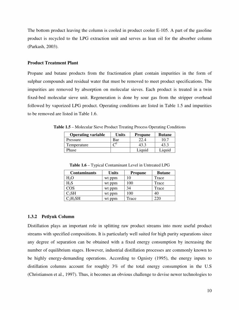
Basics of a Petlyuk Column
The Petlyuk column consists of a pre-fractionator followed by a main column from which three
product streams are obtained (Figure 1.4 (a) and (b)) (Wolff and Skogestad, 1995) and this
arrangement has been shown to provide higher energy savings than the systems with side
columns, with savings of up to 30% when compared to conventional schemes (Glinos and
Malone, 1988; Fidkowski and Krolikowski, 1990).
Figure 1.4 – Petlyuk Colom
(a) Stream notation for Petlyuk design with Pre-fractionator and main Column
(b) Practical implementation integrating. Pre-fractionator and main Column
The Petlyuk column has been studied theoretically for a considerable amount of time, but still
few of these integrated columns have been built. One of the main reasons for this is the fact that it
has many more degrees of freedom in both operation and design as compared to an ordinary
distillation column. This undoubtedly makes the design of both the column and its control system
more complex.
13
The Petlyuk design consists of a pre-fractionator with reflux and boilup from the downstream
column, whose product is fed to a 2-feed, 3-product column, resulting in a setup with only one
reboiler and one condenser. The practical implementation of such a column can be accomplished
in a single shell by inserting a vertical wall through the middle section of the column, thus
separating the feed and the side product draw (Wright, 1949). Petlyuk’s main reason for this
design was to avoid thermodynamic losses from mixing different streams at the feed tray
location. The product streams are denoted as D, S and B (and Feed F), with ternary components
1, 2 and 3.

14
2 PROJECT BASIS
2.1 Feed Streams
Feed streams used for the simulation are given in the Table 2.1. Both streams are NGL, coming
from first stage separator from well and from dehydration unit.
Table 2.1 - Feeds Streams
Property Feed 1 [from well] Feed 2 [from dehydration unit]
Temperature 25 oC 25 oC
Pressure 30 bar 30 bar
Mass flowrate 25 ton/hr 8 ton/hr
Composition (mole fraction) CH4 0.097 0.130
C2H6 0.029 0.080
C3H8 0.035 0.100
i-C4 0.018 0.055
n-C4 0.028 0.113
i-C5 0.026 0.104
n-C5 0.025 0.091
n-C6 0.064 0.122
n-C7 0.090 0.110
n-C8 0.150 0.072
n-C9 0.110 0.020
n-C10 0.090 0.003
C11 0.079 0.000
C12 0.071 0.000
C13 0.031 0.000
C14 0.023 0.000
C15 0.018 0.000
C16 0.014 0.000
H2O 0.002 0.000
2.2 Product Specifications
Product specifications are defined based on commercial products in LPG market. As described
previously, specifications of the LPG products were taken from OPIC and Argus NGL Americans
Methodology. These products can be sold on CME Group Market (NYMEX) in New York
(CME, 2010). LPG product specifications are given in the Table 2.2.

15
Table 2.2 - Product Specifications
No. Product %
Min Other
Components %
Max Relative density
Price ($/gal)
1 n-Butane 94 i-butane 6 0.584 1.54661
propane 0.35
pentane 1.5
olefin 0.35
2 i-Butane 96 n-butane 4 0.563 1.60083
propane 3
3 Propane 90 propylene 5 0.507 1.17594
4 C5+ - - - 0.664 1.90315
5 Field Grade Butane
- i-butane 35 - 1.43830
- n-butane 65
The product specification above is used as initial basis to model the simulation. However, final
decision about the product will be made after analysis of the economics of the project.
2.3 Project Scope
Simplified block flow diagram describing the project scope is shown in the Figure 2.1. Both
streams of NGL from wells and dehydration unit will be further processed through LPG recovery
unit to extract NGL into those products, propane, iso-butane, n-butane and heavier hydrocarbons
(C5+) as specified in Table 2.2 above.
There are 2 types of LPG extraction unit that will be discussed. The first one is conventional
process which separates the product step by step using several columns. The other one is using
Petyuk column. There are total 6 cases which are analyzed in this project. The alternative cases
are developed based on economic consideration to extract raw NGL into different LPG products
as shown in Table 2.3.

16
Figure 2.1 - Block Flow Diagram
Table 2.3 – Alternative Cases
Case Description Products
1 Conventional Columns Propane i-Butane n-Butane Natural Gasoline (C5+)
2 Conventional Columns Propane Butane (i-C4 + n-C4) Natural Gasoline (C5+)
3 Conventional Columns LPG (C3, i-C4 & n-C4) Natural Gasoline (C5+)
4 Petlyuk Columns Propane i-Butane n-Butane Natural Gasoline (C5+)
5 Petlyuk Columns Propane Butane (i-C4 + n-C4) Natural Gasoline (C5+)
6 Petlyuk Columns LPG (C3, i-C4 & n-C4) Natural Gasoline (C5+)

17
2.4 Assumptions
Several assumptions are used for designing this LPG recovery plant as well as simulating the
process using Unisim software.
1. Location
The LPG recovery plant will be built in Norway.
2. The LPG plant is part of gas processing plant, so that steam used for reboiler of the
column is considered to be generated as part of steam generation for the whole plant.
Then, it just needs to add the duty required to generate more steam, not to build the new
boiler for the steam.
3. In order to economise process, instead of using refrigerant it is suggested to use sea water
for condenser.
4. Sea water temperature for condenser 10oC.
5. Both conventional and petlyuk produce the same amount of the products.

18
3 PROCESS DESCRIPTIONS
In this project, LPG extraction using both conventional fractionation column and Petlyuk column
are modelled and discussed separately.
3.1 Conventional Column
Generally, the processes for 3 different cases for conventional column are the same. In this
chapter, the simulation for conventional column is done for case 1 only. This simulation also
represents case 2 and case 3 by reducing the number of the columns based on specified products.
There are 4 columns used in this conventional process. First stage of LPG extraction from NGL is
Deethanizer. In this column, methane and ethane will be separated at the top of the column as
vapor phase. The heavier hydrocarbons (C3+) will flow at the bottom in liquid phase for next
entering the Debutanizer column. In this column, propane and butane are separated and go to the
top of the column, while the stabilized natural gas liquid (C5+) flows at the bottom. In order to
obtain pure specified propane product, propane and butane are separated in Depropanizer
Column. Propane goes to the top and butane goes to the bottom. Then finally, n-butane and iso-
butane are separated in butane splitter to get the specified products.
Simplified conventional fractionation process is illustrated by Process Flow Diagram in Figure
3.1 below.
Figure 3.1 – Simplified Process Flow Diagram

19
Detailed process flow, parameter used and modelling a simulation are explained afterwards.
3.1.1 Process Flow
As described in introduction, technology and process for LPG extraction using conventional
column is typically the same as previous one. The differences are in selecting operating
conditions (pressure and temperature) of each column and arrangement of the columns. Those are
defined and determined based on feed stream conditions and composition, specifications of the
product and economics of the process. Detailed process flow diagram is shown in Figure 3.2.
The process consists of mainly four distillation columns. The specification of feeds is given in
Table 2.1. Initial feeds from both the separation units from the well and from the dehydration unit
are mixed before entering the deethanizer. In order to meet the operating pressure of deethanizer,
mixed feed (30 bar, 25oC) is expanded through expansion valve to 26 bar. Further explanation
about selecting operating pressure will be described in modeling sub-chapter 3.1.3.
In the deethanizer column, methane and ethane are expected to be separated and flow through the
top of the column. Since there is no requirement to liquefy methane and ethane, especially in
small amounts, these components will be kept in vapor phase and additional condenser is
unnecessary. The boiling point of mixed methane and ethane, in this case at pressure 18 bar, is -
52.55oC, which means that refrigerant is required to condense the gas. For economic reasons,
refrigerant will not be used in this process.
In this deethanizer, 100% methane and ethane in mixed feed can be separated and leaves the top
of the column at 18 bar and 37.53oC. This product will be used internally as a fuel to generate the
steam which is used for reboiler of the column. Heat is supplied to the column by forced
circulation using reboiler pump P-101 to reboiler E-101 and into the column. The heavier
hydrocarbons other than ethane leave the column as bottom product in liquid phase at 26 bar and
246.7oC. Next it is sent to debutanizer column.
Since the bottom product of deethanizer composed of small amount of propane (2 % of mass
fraction) and butane (5 % of mass fraction), debutanizer is used instead of depropanizer. So that
smaller columns will be used for next extraction. This is not only for economic reason, but also

20
for efficiency of the separation as it is easier to extract the product this way and less duty will be
required for reboiler E-102.
Before entering debutanizer column, the deethanizer bottom product is expanded from 26 bar to
17 bar and fed into debutanizer as mixed-phase feed. This feed is fractionated into mixed propane
and butane as overhead product and heavier hydrocarbons (C5+) as bottom product. Then the
overhead product is totally condensed in the condenser E-103 by heat exchange with cooling
water, and condensate is collected in reflux drum D-101. The cooling water is sea water with
temperature 10oC. The reflux drum should be used in order to prevent cavitation on the pump due
to vapor phase. The debutanizer reflux and product pump P-103 serve the dual purpose of
supplying reflux to the column and allowing withdrawal of column overhead product butane from
the reflux drum. The column heat is supplied by a reboiler E-102, and circulation is aided by
debutanizer reboiler circulating pump P-102.
About 100% propane and 99% butane can be recovered from the feed at the overhead column
product. This stream leaves the column at 16 bar and 76.75oC and is sent to depropanizer column
to separate propane and butane. Meanwhile, the bottom product composed of pentane and heavier
hydrocarbons will be stored as natural gasoline. Since the bottom product has high temperature
(252.3oC), it will be cooled by heat exchanger E-108 before being sent to the storage.
Propane and butane stream is expanded from 16 bar to 10 bar and enters the depropanizer as
mixed-phase feed. The depropanizer separates propane as overhead product and butane as bottom
product. Condenser E-105 is used to totally condense the overhead vapor from depropanizer. Sea
water is used for cooling. Condensate is collected in depropanizer column reflux drum D-102. A
part of the condensed overhead product is sent back to the column as reflux via pump P-105
while the remaining part is withdrawn as a liquid propane product. Depropanizer reboiler heat is
supplied by reboiler E-104. Reboiler circulation is aided by reboiler circulation pump P-104.
It is about 99.9% of propane can be recovered as top product and 99.9% of butane is recovered as
bottom product. The butane product is field grade butane which is composed of 34% i-butane and
65% n-butane. This is next being sent to butane splitter to get i-butane and n-butane products
separately, since it could be sold with higher price than field grade butane.

21
The field grade butane is expanded from 10 bar to 5 bar before enter the butane splitter. I-butane
is recovered as overhead product and n-butane as bottom product. I-butane is totally condensed
by condenser E-107. Condensate is collected in reflux drum D-103. A part of the condensed
overhead product is sent back to the column as reflux via pump P-107 while the remaining part is
withdrawn as a liquid i-butane product. Butane splitter heat is supplied by reboiler E-106.
Reboiler circulation is aided by reboiler circulation pump P-106.
Butane splitter column separates 96% mole of i-butane in the overhead product and 96% mole of
n-butane in the bottom product. Both products have higher price than field grade butane. The
whole process flow diagram is shown in Figure 3.2 below.
Figure 3.2 - Process Flow Diagram
3.1.2 Parameters
Modelling and simulating the LPG extraction process flow above is not as simple as the
description, especially to converge the distillation column with Unisim. The parameters below
should be considered in order to find a good result of simulation and the process as well as
minimize the errors of the calculation.
• Operating pressure of the column

22
• Temperature of top product – avoid using refrigerant
• Number of stages
• Column specification
• Temperature profile at each tray
• Product specification
• Reboiler duty
3.1.3 Modelling
Generally, the process modelling for LPG extraction with Unisim is divided into 5 main sections.
Those are feed conditioning, deethanizer, debutanizer, depropanizer and butane splitter. The
additional condenser and reboiler are also explained separately. Each section will be described
step by step below.
Feed Conditioning
As mentioned in the project basis, there are 2 feed streams of NGL. The compositions and
conditions of both streams are given. Feed streams are natural gas liquids that come from first
stage of separation unit from well stream (feed 1) and from dehydration unit (feed 2). Both
streams have the same condition of pressure and temperature, that is 25 oC and 30 bar, but
different compositions and mass flow rates. These NGL feeds will be extracted into 3 LPG
products, propane, iso-butane and n-butane. The products were selected based on demand in LPG
market. Furthermore, specifications of each product were determined referring to current
commercial prices.
First step of the LPG extraction process is feed conditioning before entering the deethanizer
column. Regarding feeds composition which still contains 22.7 % mole and 10.9 % mole of
methane and ethane, there are 3 alternatives for conditioning. First alternative is to mix both feeds
and expand the mixed feed to a certain pressure. Then use a separator to remove lighter
hydrocarbons. The lighter hydrocarbons are expected methane and ethane. The process is
illustrated in Figure 3.3. This alternative requires one separator vessel with capacity 33 ton/hr.
23
Figure 3.3 – Feed Conditioning Alternative 1
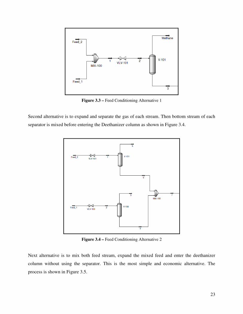
Second alternative is to expand and separate the gas of each stream. Then bottom stream of each
separator is mixed before entering the Deethanizer column as shown in Figure 3.4.
Figure 3.4 – Feed Conditioning Alternative 2
Next alternative is to mix both feed stream, expand the mixed feed and enter the deethanizer
column without using the separator. This is the most simple and economic alternative. The
process is shown in Figure 3.5.
24
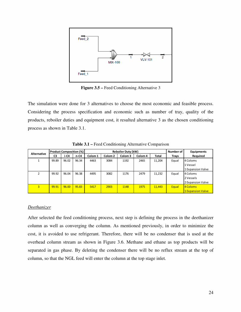
Figure 3.5 – Feed Conditioning Alternative 3
The simulation were done for 3 alternatives to choose the most economic and feasible process.
Considering the process specification and economic such as number of tray, quality of the
products, reboiler duties and equipment cost, it resulted alternative 3 as the chosen conditioning
process as shown in Table 3.1.
Table 3.1 – Feed Conditioning Alternative Comparison
C3 i-C4 n-C4 Colom 1 Colom 2 Colom 3 Colom 4 Total
1 99.89 96.02 96.34 4463 3084 1192 2465 11,204 Equal 4 Coloms
1 Vessel
1 Expansion Valve
2 99.92 96.04 96.38 4495 3082 1176 2479 11,232 Equal 4 Coloms
2 Vessels
2 Expansion Valve
3 99.91 96.00 95.83 5417 2903 1148 1975 11,443 Equal 4 Coloms
1 Expansion Valve
AlternativeProduct Composition (%) Equipments
Required
Reboiler Duty (kW) Number of
Trays
Deethanizer
After selected the feed conditioning process, next step is defining the process in the deethanizer
column as well as converging the column. As mentioned previously, in order to minimize the
cost, it is avoided to use refrigerant. Therefore, there will be no condenser that is used at the
overhead column stream as shown in Figure 3.6. Methane and ethane as top products will be
separated in gas phase. By deleting the condenser there will be no reflux stream at the top of
column, so that the NGL feed will enter the column at the top stage inlet.

25
Figure 3.6 – Deethanizer Column
First step to do after defined stream connection is selecting the operating pressure at the top and
the bottom of the column. As initial guess, 26.9 bar pressure was used based on reference. Since
the feed pressure is 30 bar, expansion valve is added in order to meet the operating pressure of the
column. Afterwards select the parameter which will be used as column specification to converge
the deethanizer column. In this case, since condenser is not used, there will be only one column
specification needs to be defined to converge the column.
Selecting operating pressure at the top and the bottom of the column is very important to separate
the methane and ethane from the NGL. The lower the pressure the more the vapour phase. The
operating pressure has to be selected so that most methane and ethane flow to overhead column
and keep propane and heavier hydrocarbons as the bottom product. The best result is to select
operating pressure 18 bar at the top stage and 26 bar at the bottom stage.
Next step is selecting the column specification. As mentioned previously, there is only one
column specification in modelling the deethanizer column. In this case, the bottom product flow
rate is selected since it is the recommended and default specification for the column. Other
specification can also be selected, for example component fraction at the top or bottom stage, but
it would be very difficult to converge the column. It depends on the composition of the feed. In
this case, the composition of methane and ethane in the feed is quite less, so that it is very
difficult to remain all the propane and heavier hydrocarbons in the bottom stage.
26
Practically, some trials have to be done to find the best result. As well as selecting operating
pressure and column specification, defining the number of stages is also quite important. The
more the number of stages means the better the separation process. In the other hand, more
number of stages means higher column is required and the cost will be more expensive.
Therefore, the number of stages has to be selected the optimum one considering both separation
efficiency and cost. As initial guess, the number of stages is defined based on reference.
In order to find the optimum number of stages, the temperature profile of each tray would help.
As well as the column converged by using initial guess of number of stages, it can be reduced to
the optimum one by considering the temperature profile of each tray. At the point where the
column is no longer converged, the previous number is selected as the optimum one. In this case,
the optimum number of stages for deethanizer is 18 stages.
After converged the column and find the optimum one based on the separation efficiency and
economic consideration, the simulation is continued to modelling the debutanizer column.
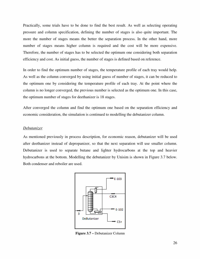
Debutanizer
As mentioned previously in process description, for economic reason, debutanizer will be used
after deethanizer instead of depropanizer, so that the next separation will use smaller column.
Debutanizer is used to separate butane and lighter hydrocarbons at the top and heavier
hydrocarbons at the bottom. Modelling the debutanizer by Unisim is shown in Figure 3.7 below.
Both condenser and reboiler are used.
Figure 3.7 – Debutanizer Column

27
Basically, the steps in modelling the debutanizer column are almost the same like modelling
deetanizer. The differences are in selecting the column specifications. Since both condenser and
reboiler are used, there are 2 column specifications to be defined in order to converge the column.
In this case, components recovery of the top product is selected as column specification. As it is
expected to separate propane and butane at the top and heavier hydrocarbons at the bottom, so
that components recovery of the propane and butane as the top product are selected.
Even though most propane and butane can be recovered as the top product, there is one
specification should be considered, that is reboiler duty. It is possible to have 99.99% of propane
and butane at the top, but more reboiler duty will be required. Thus, the fraction of components
recovery should be selected by considering minimum reboiler duty in order to minimize the cost
for the steam.
As well as modelling deethanizer, selecting operating pressure and number of stages are also
done in modelling debutanizer. Initial guess value for both specification are also based on
reference then have some trial to find the optimum value.
Depropanizer
Depropanizer is used after debutanizer column in order to separate propane and butane. The
modelling steps are almost the same with debutanizer. Both condenser and reboiler are used as
shown in Figure 3.8. In this column, propane liquid is produced as overhead product and butane
as bottom product.
Figure 3.8 – Depropanizer Column

28
Modelling the depropanizer column is simpler since it only has 2 compositions in the feed.
Components recovery is also used as column specification. There is no significant reboiler duty
difference in changing the recovery fraction value. Selecting operating pressure and number of
stages are also done using initial guess value from reference. Some trials still have to be done to
find the optimum value.
Butane Splitter
Butane from depropanizer column is next separated into i-butane and n-butane in butane splitter
column. It is typically the same as the depropanizer column as shown in Figure 3.9. Components
recovery is still used as column specification. But it is more difficult than two previous columns
to meet the products specification for n-butane and i-butane, since it is very sensitive with
changing value of component recovery. So that some trials have to be done to select the optimum
components recovery value for both n-butane and i-butane in order to meet the specification of
the product. Selecting operating pressure and number of stages are still done using initial guess
value from reference.
Figure 3.9 – Butane Splitter
The overall modelling of simulation using Unisim is shown by Figure 3.10. As mentioned
previously, this simulation represents case 1 and the other cases are illustrated in Figure 3.11 for
case 2 and Figure 3.12 for case 3.

29
Figure 3.10 – Process Flowsheet Case 1
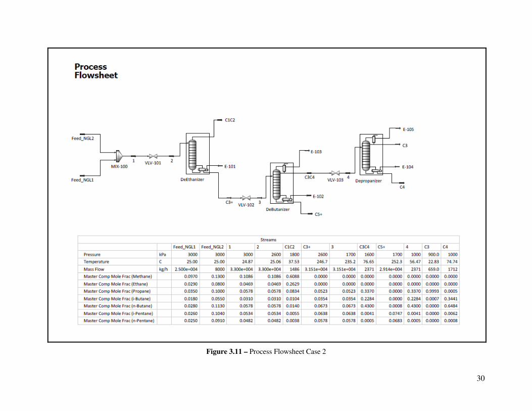
30
Figure 3.11 – Process Flowsheet Case 2

31
Figure 3.12 – Process Flowsheet Case 3

32
Reboiler and Condenser
Reboiler and condenser are parts of the columns. Reboiler is used to supply heat into the column,
so that the lighter hydrocarbons will be vaporized and go up to the top stage. Steam is used to
heat up a part of bottom product and recycle it into the column. Meanwhile, condenser is used to
condense the overhead vapor so the liquid product will be produced which partially recycled into
the column as reflux.
In simulation, as part of a distillation column, both reboiler and condenser are defined based on
requirement in order to meet product specifications.
Recirculation Pumps
Recirculation pump is used to recycle the reflux and heat supply into the column. It is not shown
in the simulation but still need to be calculated for the cost estimation.

33
3.2 Petlyuk Column
3.2.1 Minimum Energy Mountain Diagram
The starting point for Petlyuk column simulations is to plot Minimum Energy Mountain Diagram.
Minimum Energy Mountain Diagram or just Vmin-diagram is introduced to effectively visualize
how the minimum energy consumption is related to the feed component distribution for all
possible operating points.
A main result is a simple graphical visualization of minimum energy and feed component
distribution. The assumptions are constant relative volatilities, constant molar flows constant and
infinite number of stages (Halvorsen and Skogestad, 2002).
Underwood equation
For a multicomponent mixture the vapor flow rate for a given separation can be calculated using
Underwood’s equations. The minimum vapor flow rate at the top of the column is given as
(Engelien and Sigurd Skogestad, 2005):
The common Underwood roots are given as the N-1 solutions of the feed equation:
,
The solutions obeys
K-values and Relative Volatility
The K-value (vapor-liquid distribution ratio) for a component i is defined as:
,
The relative volatility between components i and j is defined as:
,

34
K value depends strongly on temperature and pressure. DePriester charts can be used to
determine K value.
In addition, it is possible to apply rough empirical formula to estimate relative volatility.
,
where ,
,
If know is unknown, a typical value can be used for many cases (Halvorsen and
Skogestad, 1999). But in practice it easier to take K-values directly from Hysys or Unisim.
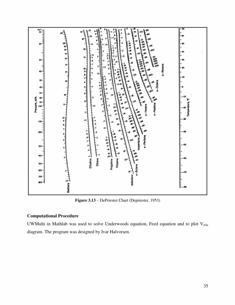
35
Figure 3.13 – DePriester Chart (Depriester, 1953)
Computational Procedure
UWMulti in Mathlab was used to solve Underwoods equation, Feed equation and to plot Vmin
diagram. The program was designed by Ivar Halvorsen.
36
Table 3.2 – K values, Relative Volatilities and Composition of the Feed
Component K values Relative volatilities zf
CH4 9.919368675 13635622.5 8.66E-02
C2H6 1.965425837 2701765.2 4.46E-02
C3H8 0.585428568 804757.2 5.81E-02
i-C4 0.242096011 332796.4 3.16E-02
n-C4 0.174953747 240499.5 5.92E-02
i-C5 7.27E-02 99990.6 5.49E-02
n-C5 5.52E-02 75918.4 4.96E-02
n-C6 1.81E-02 24888.0 8.70E-02
n-C7 6.16E-03 8474.7 1.00E-01
n-C8 2.11E-03 2900.2 0.1265589
n-C9 7.56E-04 1039.1 8.09E-02
n-C10 2.79E-04 382.9 6.14E-02
C11 9.90E-05 136.1 5.29E-02
C12 4.09E-05 56.2 4.76E-02
C13 1.32E-05 18.2 2.08E-02
C14 4.06E-06 5.6 1.54E-02
C15 1.93E-06 2.7 1.21E-02
C16 7.27E-07 1.0 9.38E-03
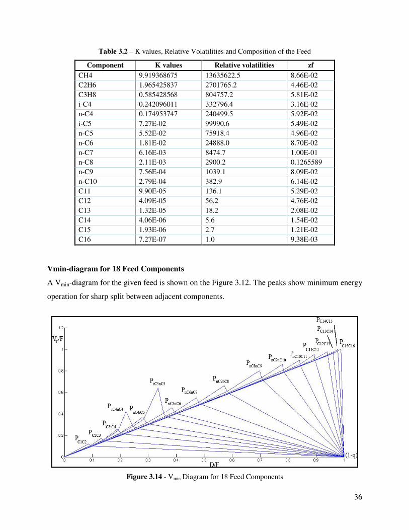
Vmin-diagram for 18 Feed Components
A Vmin-diagram for the given feed is shown on the Figure 3.12. The peaks show minimum energy
operation for sharp split between adjacent components.
Figure 3.14 - Vmin Diagram for 18 Feed Components

37
The highest peak determines the maximum minimum vapour flow requirement in the
arrangement. But in this study there is no need to separate C15 from C16, because the final
products should be LPG and NGL. It is important to separate only C1C2, C3, iC4, nC4 and C5+
from each other.
Five products in 18 component feed
In Petlyuk arrangement all columns are directly (fully thermally) coupled. The total number of
internal directly coupled two-product columns to separate M products is (M - 1) + (M - 2) + ... =
M(M - 1)/2. There are (M – 1) product splits, and these can be related to M - 1 minimum-energy
operating points (peaks) in the Vmin diagram (Halvorsen and Skogestad, 2002).
M(M - 1)/2=5*(5-1)/2=10
A – C1C2, B – C3, C – iC4, D – nC4, E – C5+
Figure 3.15 – Five Products Petlyuk Arrangement for LPG and NGL Production

38
Vmin diagram for a given 18-component feed (C1-C16) is shown in the Figure 3.14. This feed
should be separated into five procuts (C1C2, C3, iC4, nC4, C5+). The plot shows the Vmin-
diagram for the feed components (blue line) and the equivalent diagram for the products (red
line). The specification for products is shown in Table 3.3. The reason for 6% of iC4 in the nC4 is
the descreasing of Vmin energy for iC4/nC4 split. Due to the specification it is possible to obtaint
iC4 and nC4 with 96% purity.
Figure 3.16 - Assessment of Minimum Vapour Flow for Separation of a 18-Component Feed into 5
Products (C1C2, C3, iC4, nC4, C5+)
Table 3.3 – Specification of Feed Component Recoveries in Products C1C2, C3, iC4, nC4, C5+
Product Light Key
Impurity
Specification
Heavy Key
Impurity
Specification
Comments
C1C2 0% C3 All of C1, most of
C2
C3 0% C2 5% iC4 Sharp C3/iC4 split
iC4 0% C3 4% nC4
nC4 6% iC4 0%C5+
C5+ 0% 100% C5+ All heavy
components
The result of minimum energy solution for each split is given in Table 3.4. Each split gives us the
peaks and knots (Pij) in the Vmin diagram for five products (red line). The highest peak is iC4/nC4

39
split VT.min=0.4033. This is the maximum minimum vapor flow requirement in the arrangement
and it is directly related C43. All heat for vaporization has to be supplied in the bottom, but the
other peaks are lower. Column C41, C42, C44 will get a higher vapor load then required.
Table 3.4 – Minimum Energy Solution for Each Split
Split Column VT.min
ABCD/BCDE C1 0.1510
ABC/BCD C21 0.1547
BCD/CDE C22 0.2251
AB/BC C31 0.1565
BC/CD C32 0.2468
CD/DE C33 0.2954
A/B C41 0.1728
B/C C42 0.2474
C/D C43 0.4033
D/E C44 0.3720
Heat Exchangers at the Side Stream Junctions
To set all flow rates independently in columns C44, C43, C42, C41, it is possible to withdraw
liquid products and use a heat exchanger where the duty corresponds to the change in vapour
flow. This vapour change may be taken from Vmin diagram as the difference between peaks. Heat
exchangers are unnecessary at the internal feed junction, because any amount of liquid of vapor
can be taken from the succeeding column.
This scheme gives full flexibility in controlling the two degrees of freedom in each internal
column. The Vmin-diagram gives minimum vapour requirements for every section for the
specified separation, but when the peaks are different heat can be removed of supplied at the
boiling points of the intermediate components. The highest peak will set the same vapour flow
requirement through the most demanding intersection in both cases.
For columns C44 and C43 the difference between vapor flow is Vmin=0.3720-0.4033=-0.0313,
for C43 and C42 Vmin=0.1559 and it is possible to install heat exchanger between them. The
same for columns C42 and C41 with Vmin=0.0746. To sum it up with heat exchangers in the
sidestream junctions, each column is supplied with its minimum energy requirement (Halvorsen,
2001).

40
Figure 3.17 – Extended Arrangement for Five Products Petlyuk Column with Heat
Exchangers at the Sidestream Junctions
Four products in 18 component feed
Four products Petlyuk column arrangement can be used to obtain the following components:
C1C2, C3, iC4nC4, C5+. The difference with the previous five products arrangement is in the
combination of iC4 and nC4 in one product. It may be dictated by economic situation.
For this case the total number of internal directly coupled columns will be 4*(4-1)/2=6. Four
products Petlyuk column is shown on the Figure 3.16.

41
A – C1, C2 ; B – C3 ; C – iC4, nC4 ; D – C5+
Figure 3.18 – Four products Petlyuk Arrangement for LPG and NGL Production
To decrease minimum energy for iC4nC4/C5 split the heavy key impurity C5+ in iC4nC4 is
specified to 5%. In this case the saparation of iC4/nC5 is avoided. The new Vmin diagram for four
products is shown on the Figure 3.17.
Table 3.5 – Specification of Feed Component Recoveries in Products C1C2, C3, iC4nC4, C5+
Product LK Impurity
Specification
HK Impurity
Specification Comments
C1C2 0% C3 All of C1, most of C2
C3 0% C2 5% iC4nC4 Sharp C3/iC4 split
iC4nC4 0% C3 1% C5+
C5+ 1% iC4nC4 99% C5+ All heavy components

42
Figure 3.19 - Assessment of Minimum Vapour Flow for Separation of a 18-Component Feed into 4
Products (C1C2, C3, iC4nC4, C5+).
The resulting minimum-energy solution for each split is given in the Table 3.6. The highest peak
is iC4nC4/C5+ split VT.min = 0.3559. This is the maximum minimum vapor flow requirement in
the arrangement and it is directly related C33.
Table 3.6 – Minimum Energy Solution for Each Split
Split Column VT.min
ABC/BCD C1 0.1547
AB/BC C21 0.1565
BC/CD C22 0.2468
A/B C31 0.1728
B/C C32 0.2474
C/D C33 0.3559
3.2.2 Modelling and Simulation of Petlyuk Columns
The main idea of revisiting the idea of Petlyuk column was to be able to simulate a Petlyuk
column as an alternative to the use of conventional columns as described in Chapter 3. The
driving force behind this was the fact that theoretical studies have shown that such an
arrangement can save, on average, around 30% of energy cost compared to conventional
arrangement.

43
Thus, the specifications mentioned in Table 2.2 were set as the required product specifications
from the Petlyuk Column (Unisim simulation), highlighted in Figure 3.18 and internal column
configuration (Unisim simulation) shown in Figure 3.19.
Figure 3.20 – Unisim Simulation of LPG Plant Using Petlyuk Column
Figure 3.21 – Unisim Simulation Showing Petlyuk Column Internal Configuration
44
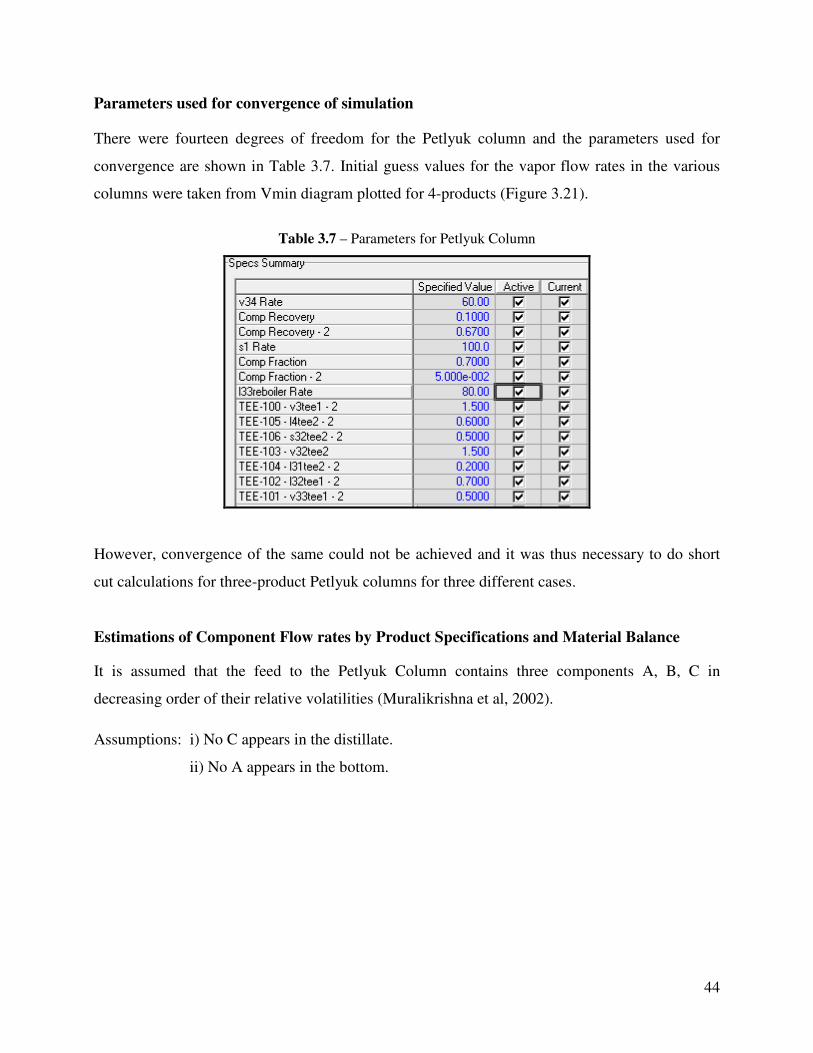
Parameters used for convergence of simulation
There were fourteen degrees of freedom for the Petlyuk column and the parameters used for
convergence are shown in Table 3.7. Initial guess values for the vapor flow rates in the various
columns were taken from Vmin diagram plotted for 4-products (Figure 3.21).
Table 3.7 – Parameters for Petlyuk Column
However, convergence of the same could not be achieved and it was thus necessary to do short
cut calculations for three-product Petlyuk columns for three different cases.
Estimations of Component Flow rates by Product Specifications and Material Balance
It is assumed that the feed to the Petlyuk Column contains three components A, B, C in
decreasing order of their relative volatilities (Muralikrishna et al, 2002).
Assumptions: i) No C appears in the distillate.
ii) No A appears in the bottom.

45
Figure 3.22 – Internal Configuration of 4-Products Petlyuk Column
In general, specifications are made on the following product compositions:
xD,A, xM,B, xB,C,
The seven unknown variables related to the output of the column are:
The equations resulting from the specifications are:
(1)
(2)
(3)
(4)
46
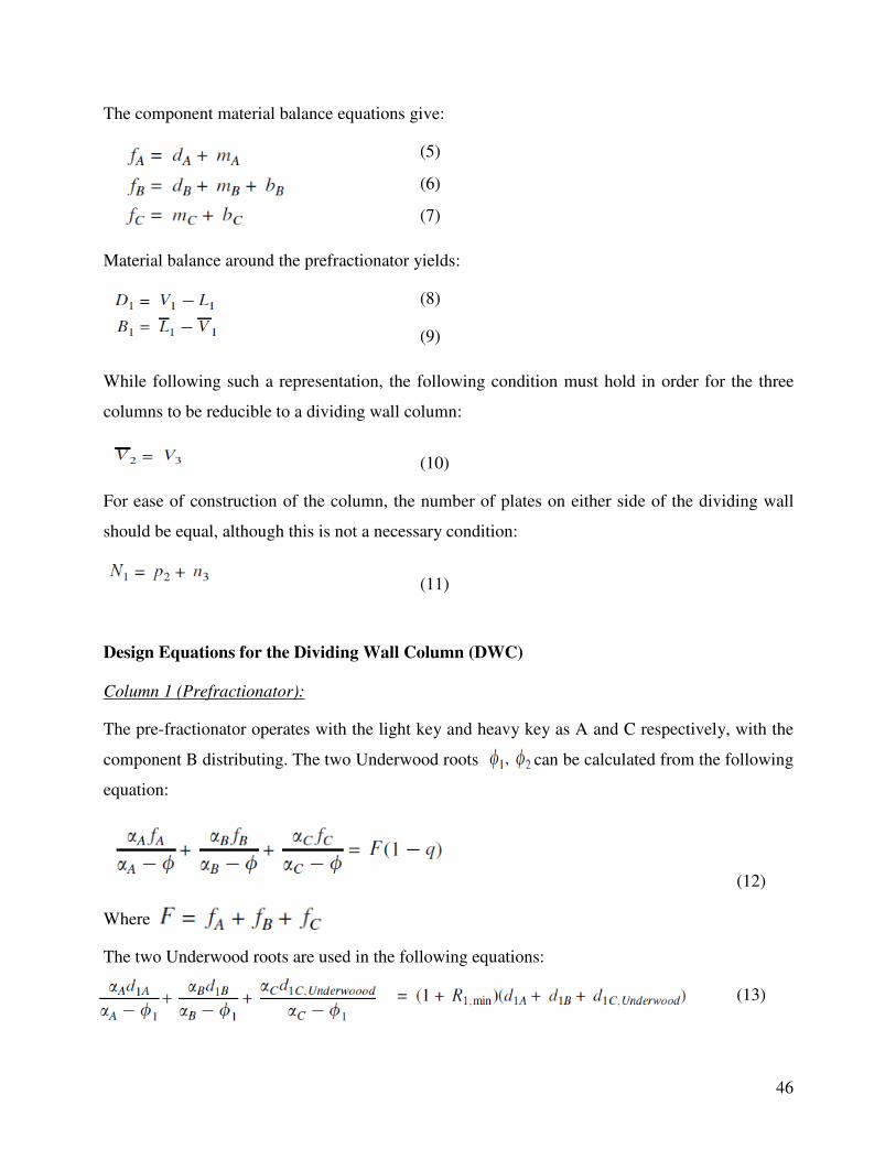
The component material balance equations give:
(5)
(6)
(7)
Material balance around the prefractionator yields:
(8)
(9)
While following such a representation, the following condition must hold in order for the three
columns to be reducible to a dividing wall column:
(10)
For ease of construction of the column, the number of plates on either side of the dividing wall
should be equal, although this is not a necessary condition:
(11)
Design Equations for the Dividing Wall Column (DWC)
Column 1 (Prefractionator):
The pre-fractionator operates with the light key and heavy key as A and C respectively, with the
component B distributing. The two Underwood roots can be calculated from the following
equation:
(12)
Where
The two Underwood roots are used in the following equations:
(13)

47
(14)
d1A, d1B are specified and then the values of d1C,Underwood and R1,min can be calculated.
(15 a)
if R.H.S of 15(a) > 0
= 0 (15 b)
if R.H.S of 15(a) < 0
From equations (13) and (15), we get the value R1,min as
(16)
At total reflux:
Fenske equation gives the minimum number of theoretical stages for a specified separation. The
equation can be written for any pair of components, provided they distribute between the distillate
and the bottoms.
For a given d1A, d1B , the Fenske equation reduces to:
(17)
And
(18)

48
Hence, for a given (d1A, d1B ) d1C, Fenske can be calculated by evaluating the right hand sides of
Equations (17) and (18):
(19)
At finite reflux:
Once, the flow rates of C in the distillate at minimum and infinite reflux have been found out, the
flow rate of C in the distillate of Column 1 at a finite reflux ratio R1 greater than the minimum,
can be found out
(20)
Thereafter, Gilliland Correlation may be used to determine the actual number of stages in Column
1:
(21)
(22)
(23)
Having known d1A, d1B and d1C, b1A, b1B and b1C can be found out by using:
(24)
(25)
(26)
The vapour flows in the rectifying and the stripping sections of the column can be found out as:
49
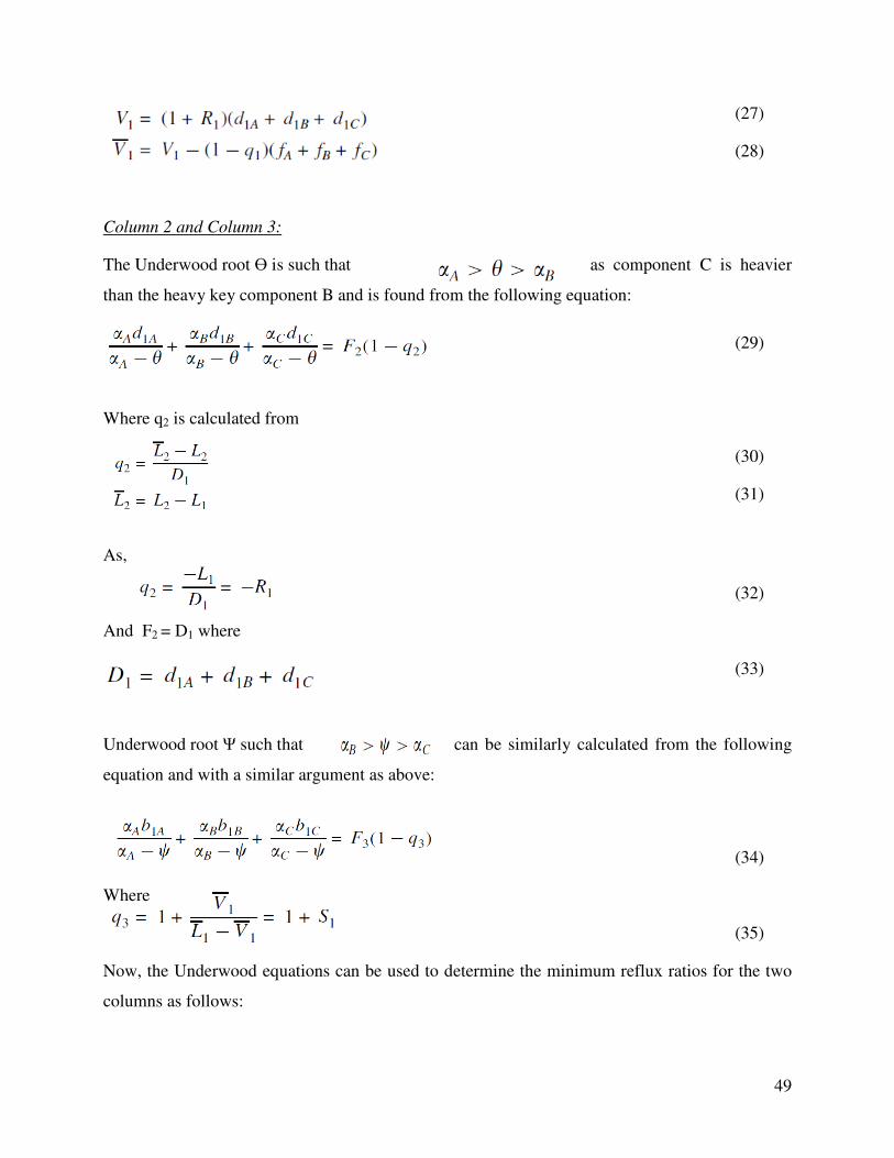
(27)
(28)
Column 2 and Column 3:
The Underwood root Ө is such that as component C is heavier
than the heavy key component B and is found from the following equation:
(29)
Where q2 is calculated from
(30)
(31)
As,
(32)
And F2 = D1 where
(33)
Underwood root Ψ such that can be similarly calculated from the following
equation and with a similar argument as above:
(34)
Where
(35)
Now, the Underwood equations can be used to determine the minimum reflux ratios for the two
columns as follows:
50
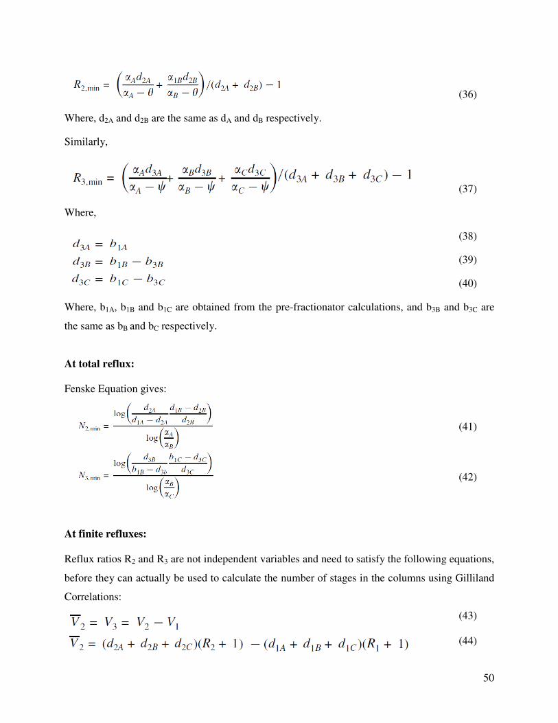
(36)
Where, d2A and d2B are the same as dA and dB respectively.
Similarly,
(37)
Where,
(38)
(39)
(40)
Where, b1A, b1B and b1C are obtained from the pre-fractionator calculations, and b3B and b3C are
the same as bB and bC respectively.
At total reflux: Fenske Equation gives: (41) (42)
At finite refluxes: Reflux ratios R2 and R3 are not independent variables and need to satisfy the following equations,
before they can actually be used to calculate the number of stages in the columns using Gilliland
Correlations:
(43) (44)

51
(45) Substituting equations 44 and 45 in equation 43, we get: (46) Gilliland correlations as in the previous can now be used to compute the number of stages in the
Columns 2 and 3 for a chosen R2 and R3.
A check is made whether the condition demonstrated by equation 11 is satisfied or else an
iterative approach is used for refining the guessed R2 and R3.
Results of Short Cut Calculations
The short cut calculations illustrated above have been used to compute the number of stages in
the pre-fractionator and the two columns for the 3 different cases. Detailed calculations are
presented in Appendix C.
However, the number of stages N1, N2 and N3 calculated using the above equations were quite
small compared to real life scenario. This may be attributed to the fact that in real distillation
problems, relative volatilities change along the height of the column, Petlyuk columns operate
under semi-vacuum pressures and the influence of dividing wall on the number of stages. Thus
the actual number of stages for the Petlyuk Column is taken as ‘k’ times the minimum number of
stages. The value of k is chosen smaller for Case 4 owing to relatively lesser reflux ratios
compared to the other two cases. The same values for the three cases are tabulated in Table 3.8.
Table 3.8 – Petlyuk Column Calculation Results for 3 Cases
Case N1,min N2.min N3,min k Actual Number of trays
Case 4 5.2806 6.99 21.23 2.5 84
Case 5 7.8232 16.39 6.34 3.0 92
Case 6 2.5982 3.50 3.17 3.0 29
52
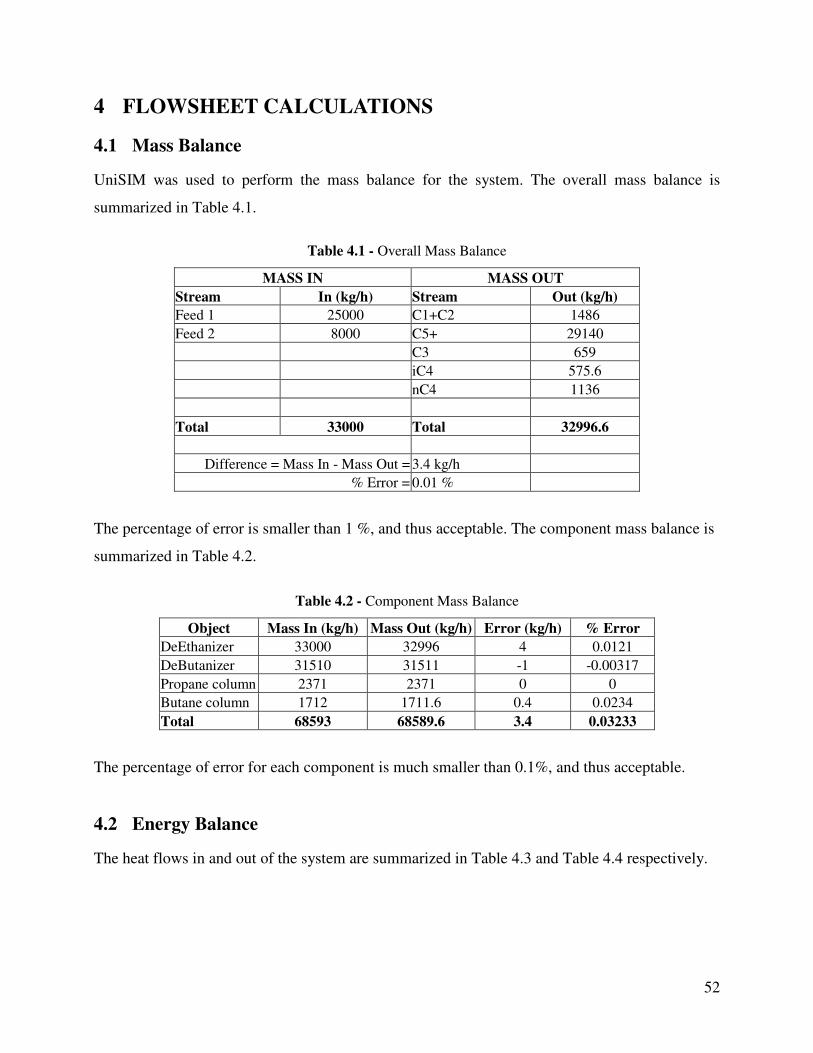
4 FLOWSHEET CALCULATIONS
4.1 Mass Balance
UniSIM was used to perform the mass balance for the system. The overall mass balance is
summarized in Table 4.1.
Table 4.1 - Overall Mass Balance
MASS IN MASS OUT
Stream In (kg/h) Stream Out (kg/h)
Feed 1 25000 C1+C2 1486
Feed 2 8000 C5+ 29140
C3 659
iC4 575.6
nC4 1136
Total 33000 Total 32996.6
Difference = Mass In - Mass Out = 3.4 kg/h
% Error = 0.01 %
The percentage of error is smaller than 1 %, and thus acceptable. The component mass balance is
summarized in Table 4.2.
Table 4.2 - Component Mass Balance
Object Mass In (kg/h) Mass Out (kg/h) Error (kg/h) % Error
DeEthanizer 33000 32996 4 0.0121
DeButanizer 31510 31511 -1 -0.00317
Propane column 2371 2371 0 0
Butane column 1712 1711.6 0.4 0.0234
Total 68593 68589.6 3.4 0.03233
The percentage of error for each component is much smaller than 0.1%, and thus acceptable.
4.2 Energy Balance
The heat flows in and out of the system are summarized in Table 4.3 and Table 4.4 respectively.

53
Table 4.3 – Heat flows in to the system Table 4.4 – Heat flows in to the system
Streams In Heat Flow (107 kJ/h)
Streams Out Heat Flow (107 kJ/h)
Feed 1 -5.499 C1C2 -0.5202
Feed 2 -1.986 C5 -4.515
E-101 1.95 C3 -0.1798
E-102 1.045 Ic4 -0.152
E-104 0.4132 Nc4 -0.282
E-106 0.7112 E-103 -1.133
E-105 0.4251
E-107 0.7257
Total -3.3656 Total -3.3652
Heat flow in – Heat flow out = -3.3656x 10⁷ kJ/h – (-3.3652) x 107 kJ/h = -0.0004 x 10⁷ kJ/h The percentage of error is 0.01189 %, which is acceptable.
Table 4.5 – Component Heat Balance
Object Heat In
(107 kJ/h) Heat Out (107 kJ/h)
Error (107 kJ/h)
% Error
DeEthanizer -5.535 -5.5362 0.0012 -0.022
DeButanizer -3.971 -3.9694 -0.0016 0.04
Propane column -0.1742 -0.1742 0 0
Butane column 0.2917 0.2917 0 0
Total -9.3885 -9.3881 0.0001 0.018
4.3 Equipment Sizing
The main equipment used in the process is summarized in Table 4.6 and Table 4.7. For details
about the calculation, see Appendix B.
Table 4.6 – Main Equipment I
Description Height/length
[m] Diameter
[mm] # Trays
Trays Space [m]
Thickness [mm]
Deethanizer 21.6 1600 30 0.6 8
Debutanizer 33.84 1400 47 0.6 6.35
Depropanizer 20.4 1000 34 0.5 6.35
Butane Splitter 25.2 1000 42 0.5 6.35

54
Table 4.7 – Main Equipment II
Table 4.8 – Other Equipments
Name Tag Description
V-101 Deethanizer Expansion Valve
V-102 Debutanizer Expansion Valve
V-103 Depropanizer Expansion Valve
V-104 Butane Splitter Expansion Valve
P-101 Deethanizer Reboiler Circulation Pump
P-102 Debutanizer Reboiler Circulation Pump
P-103 Debutanizer Condenser Circulation Pump
P-104 Depropanizer Reboiler Circulation Pump
P-105 Depropanizer Condenser Circulation Pump
P-106 Butane Splitter Reboiler Circulation Pump
P-107 Butane Splitter Condenser Circulation Pump
D-101 Debutanizer Reflux Drum
D-102 Depropanizer Reflux Drum
D-103 Butane Splitter Reflux Drum
T-101 Methane and Ethane Storage Tank
T-102 Natural Gasoline Storage Tank
T-103 Propane Storage Tank
T-104 i-Butane Storage Tank
T-105 n-Butane Storage Tank
E-108 Natural Gasoline Condenser
Description Tag Duty [kW] Surface area [m2] Type
Deethanizer Reboiler E-101 5414 573.6 Kettle
Debutanizer Reboiler E-102 2907 445.5 Kettle
Depropanizer Reboiler E-104 1166 35.9 Kettle
Butane Splitter Reboiler E-106 1976 55.5 Kettle
Debutanizer Condenser E-103 3148 361 Shell and tube
Depropanizer Condenser E-105 1199 1141 Shell and tube
Butane Splitter Condenser E-107 2016 864 Shell and tube

55
5 COST ESTIMATION
5.1 Fixed capital cost
The fixed capital cost is estimated to get an approximate price for the total plant installed and
running. These calculations are based on given percentages (West, Ronald E., et al, 2003). Major
equipment costs are calculated as describes in Appendix E. The major costs for different cases are
shown in the tables below.
Table 5.1 - Major Equipment Cost of Case 1*
Equipment Cost ($) Column 425571.51
Tray 60651.54
Heat exchangers 29157889.63
Tank 340002.30
Pump 141088.33
Major equipment cost 30705203.31
* Equipment number in case 1: 4 columns, 109 column trays, 7 heat exchangers, 5 tanks and 3 pumps
Table 5.2 - Major Equipment Cost of Case 2*
Equipment Cost ($) Column 363798.73
Tray 420259.99
Heat exchangers 21992155.77
Tank 261950.94
Pump 105377.44
Major equipment cost 23143542.86
* Equipment number in case 2: 3 columns, 79 column trays, 5 heat exchangers, 4 tanks and 2 pumps
Table 5.3 - Major Equipment Cost of Case 3*
Equipment Cost ($) Column 332369.64
Tray 325525.98
Heat exchangers 10626537.25
Tank 189908.08
Pump 61737.53
Major equipment cost 11536078.49
* Equipment number in case 3: 2 columns, 55 column trays, 3 heat exchangers, 3 tanks and 1 pump

56
Table 5.4 - Major Equipment Cost of Case 4*
Equipment Cost ($) Column 437508.85
Tray 714012.12
Heat exchangers 17494733.78
Tank 300389.13
Pump 91761.83
Major equipment cost 19038405.72 * Equipment number in case 4: 3 columns, 139 column trays, 5 heat exchangers, 5 tanks and 2 pumps
Table 5.5 - Major Equipment Cost of Case 5*
Equipment Cost ($) Column 288814.33
Tray 565991.48
Heat exchangers 13973566.09
Tank 285109.76
Pump 39031.59
Major equipment cost 151552512.25 * Equipment number in case 5: 2 columns, 122 column trays, 3 heat exchangers, 4 tanks and 1 pump
Table 5.6 - Major Equipment Cost of Case 6*
Equipment Cost ($) Column 88218.72
Tray 331447.72
Heat exchangers 11607252.13
Tank 64754.35
Pump 80258.79
Major equipment cost 12171931.71 * Equipment number in case 6: 1 columns, 28 column trays, 2 heat exchangers, 3 tanks and 1 pump
The fixed capital costs for different cases are listed in Tables 5.7. The cost estimation of Petlyuk
columns has been done similarly, using 1.6 times the investment cost of an equi-sized
conventional column. The factor takes into account costs of dividing wall, thicker shell and other
unknown costs.

57
Table 5.7 - Fixed Capital Cost for Different Cases
Fixed Capital cost
Percent of delivered
equipment cost
Cost (MUSD)
Case1 Case2 Case3 Case4 Case5 Case6
Purchased equipment delivered, E
100 30.71 23.14 11.54 19.04 15.15 12.17
Purchased equipment installation
47 14.43 10.88 5.42 8.95 7.12 5.72
Instrumentation and controls (installed)
36 11.05 8.33 4.15 6.85 5.45 4.38
Piping (installed) 68 20.88 15.74 7.84 12.95 2.56 2.06
Electrical systems (installed)
11 3.38 2.55 1.27 2.09 1.96 1.58
Buildings (inclduing servics)
18 5.53 4.17 2.08 3.43 0.92 0.74
Yard improvements
10 3.07 2.31 1.15 1.90 0.71 0.57
Services facilities (installed)
70 21.49 16.20 8.08 13.33 0.33 0.27
Engineering and supervision
33 10.13 7.64 3.81 6.28 5.00 4.02
Construction expenses
41 12.59 9.49 4.73 7.81 6.21 4.99
Legal expenses 4 1.23 0.93 0.46 0.76 0.61 0.49
Contractor's fee 22 6.76 5.09 2.54 4.19 3.33 2.68
Contingency 44 13.51 10.18 5.08 8.38 6.67 5.36
Fixed capital
investment 154.75 116.64 58.14 95.95 56.04 45.02
5.2 Working capital cost
The working capital is the amount of capital required to start up the plant and to finance the first
couple of months of operating before the plant starts earning, this capital is used to cover salaries,
raw material inventories and contingencies. It will be recovered at the end of the project and
represents a float of money to get the project started. These costs are necessary at start-ups and it
implies raw materials and intermediates in the process. The working capital was assumed to be
3% of the fixed capital cost (West, Ronald E., et al, 2003). The total investment for the plant is
listed in Table 5.8.
58
Table 5.8 - The Total Investment
Investment Cost (MUSD)
Case1 Case2 Case3 Case4 Case5 Case6 Fixed capital cost
154.75 116.64 58.14 95.95 56.04 45.02
Working capital cost
4.64 3.50 1.74 2.88 1.68 1.35
Total investment
159.40 120.14 59.89 98.83 57.72 46.37
5.3 Operating Cost
All expenses directly connected with the manufacturing operation or the physical equipment of a
process plant itself are included in the operating costs (Peters, 1991). Operating costs are divided
into three categories: direct manufacturing costs, fixed manufacturing costs and general expenses.
Direct manufacturing costs represent operating expenses that vary with production rate. When
product demand drops, production rate is reduced to less than the design capacity. A reduction in
the factors making up the direct manufacturing costs is observed.
Fixed manufacturing costs are independent of changes in production rate. They include property
taxes, insurance and depreciation, which are charged at constant rates even when the plant is not
in operation.
General expenses represent an overhead burden that is necessary to carry out business functions.
They include management, sales, financing, and research functions. General expenses seldom
vary with production level (Turton, 2008).
Direct Costs
Raw materials costs
The raw materials in the process are natural gas liquids (NGL) and steam.
Natural Gas Liquids
The price for 1MBtu is 7USD (for 1000 cubic foot of NG). It is necessary to calculate the price
for Raw NGL Feed for the plant. The Lower Heating Value in the Feed Stream is 4.264*106
KJ/kgmole. To make heating value in KJ/m3 it should be multiplied by molar density:

59
Heating value = 4.264*106*5.746=24.5*106 KJ/m3 [KJ/kgmole * kgmole/m3=KJ/m3]
The value 24.5*106 KJ/m3 corresponds to 23.221 MBtu/m3. It means that one m3 of Raw Feed
can produce 23.221 MBtu of energy. So, 0.0431 m3 of Raw Feed will produce 1 MBtu of energy
and this amount of energy costs apporximately 7 USD.
If 43.1 liters of Raw Feed costs 7USD, then 158.9 liters of Raw feed costs 25.8USD. So, one
barrel of Raw Feed will cost 25.8USD (or 0.3USD per kg). The price for product (natural
gasoline) is 67.3 USD/Bbl. It is possible to assume that the real price will be 20% higher and
equals to 31 USD/bbl (or 0.36 USD per kg). Annual raw NGL feed cost:
Feed 1 = 25000 kg * 24 * 360 * 0.36$ = 77.76 MUSD/Year,
Feed 2 = 8000 kg * 24 * 360 * 0.36$ = 24.883 MUSD/Year,
Total Feed cost = 102.643 MUSD/Year.
Steam
It was assumed that this plant is supplied by steam from another industrial producer. The cost of
high pressure steam is 29.97 USD/tonne (Turton, 2009). The necessary amount of high pressure
steam is shown in the Table 5.9.
Table 5.9 – The Amount of Steam and Price
Case Steam Flow Rate, tonnes/h Price, MUSD/year
Conventional Columns
1 514.974 130.233
2 424.713 107.407
3 372.511 96.458
Petlyuk Column
4 394.296 102.099
5 326.937 84.657
6 286.547 74.199

60
Utility prices
Utilities prices consist of the process natural gas and the electricity for cooling water pumping.
Natural Gas
This plant produces natural gas (methane and ethane). The internal price for natural gas in Statoil
ASA is shown on the Figure 5.1. An average price for last 4 years is 0.23 $/Sm3 (or 1.44
NOK/Sm3). It will be used for the entire operating period.
Annual price for gas = 1444.2 Sm3/h * 24 * 360 * 0.23 $/Sm3 = 2.867 MUSD/Year.
It is possible to earn 2.867 MUSD/Year by selling gas from the LPG recovery plant.
Figure 5.1 – The Internal Price for Natural Gas in Statoil
Cooling water
The price of electric power for the industry in Norway is given in the Figure 5.2 (Statistics
Norway, 2010). The price is assumed to be constant and equal to 0.05 $/kWh throughout the
whole period of production.

61
Figure 5.2 – Electric Power Prices in Norway
The cost of the cooling water is the cost of pumping the cooling water through the system, costs
for water make-up and chemical treatment of the water. As shown in Figure 5.3 the pumping cost
is assumed to be 0.01$ per 1m3 of water per hour. The pumping cost for 6 cases is summarized in
Table 5.10.
Figure 5.3 – Pumping Cost

62
Table 5.10 – The Amount of Water and Pumping Cost (for Petlyuk assumed 20% less)
Case Water flow rate, m3/h Price, MUSD/year
Conventional Columns
1 362.349 0.031
2 187.982 0.016
3 87.727 0.0076
Petlyuk Column
4 289.879 0.024
5 150.386 0.0128
6 70.181 0.0061
Operating labor
The following formula may be used for labor requirements estimations:
NOL = (6.29+31.7P2+0.23Nnp)0.5,
where NOL is the number of operators per shift,
P is the number of processing steps (for example, transportation and distribution),
Nnp is the number of nonparticulate processing steps and includes compression, heating, cooling,
mixing. Four and one-half operators are hired for each operator needed in the plant any time
(Turton, 2008).
For the first case there are four distillation towers in the process, seven heat exchangers and five
tanks so Nnp=16.
NOL=(6.29+0.23 * 16)0.5=3.16 operator per shift.
Operating labour = 3.16 * 4.5 = 14.22 (rounding to the nearest integer gives 15)
Labor costs = 15 * 100000$/year=1.5 MUSD/Year.
Operating labour for 6 cases is tabulated in Table 5.11.

63
Table 5.11 – Operating Labour
Case Number of main
equipment
Nnp Labor
requirements, NOL
Number of
labors
Labor cost,
MUSD/Year
Conventional Columns
1 Four towers, seven heat
exchangers, five tanks 16 3.16 15 1.5
2 Three towers, five heat
exchangers, four tanks 12 3 14 1.4
3 Two towers, three heat
exchangers, three thanks 8 2.89 13 1.3
Petlyuk Column
4 Three towers, five heat
exchangers, five tanks 13 3.046 14 1.4
5 Two towers, three heat
exchangers, four tanks 9 2.89 13 1.3
6 One tower, two heat
exchangers, three thanks 6 2.77 13 1.3
The following formula was used to calculate operating cost for the plant:
This formula coefficients take into account direct manufacturing costs (raw materials, utilities,
operating labor, supervisory, maintenance and repair, laboratory charges and patents), fixed
operating costs, (depreciation, taxes and insurance, plant overhead costs), general manufacturing
expenses (administration costs, distribution and selling costs, research and development and
future worth factor).
Table 5.12 – Total Operating Cost
Case Fixed capital investment FCI,
MUSD
Raw materials CRM, MUSD/Year
Utilities CUT, MUSD/Year
Operating labor COL,
MUSD/Year
Operating cost, MUSD/Year
Conventional Columns
1 159.397 232.876 2.836 1.5 351.918
2 120.143 210.05 2.851 1.4 307.608
3 59.886 198.101 2.8594 1.3 268.178
Petlyuk Column
4 99.198 204.742 2.843 1.4 292.59
5 58.008 187.3 2.8542 1.3 254.127
6 45.606 176.842 2.8609 1.3 236.215

64
6 INVESTMENT ANALYSIS
Profitability is the measure of the amount of profit that can be obtained from a given situation. It
is as common denominator for all business activities. The determination and analysis of profits
obtainable from the investment of capital and the choice of the best investment among various
alternatives are major goals of the investment analysis (Peters, 1991).
The life time of the project was assumed to be 20 years. The depreciation for the plant is
estimated to be at 10 percent. The tax to be paid to the government is assumed to be at 38%. The
summary of investment analysis for 6 cases is shown in Table 6.1.
Table 6.1 – Performance Measurement of the Investment
Description Conventional Columns Petlyuk Column
Case 1 Case 2 Case 3 Case 4 Case 5 Case 6
IRR - - 13% - 31% 62%
NPV, M$ -781.701 -307.330 26.767 -137.529 127.356 241.557
PBP, Years - - 7.8 - 3.5 1.8
The Cases 1,2 and 4 yielded negative IRR and NPV, because they have negative annual cash
flows and are thus unprofitable.
6.1 Internal Rate of Return
The internal rate of return on an investment or project is the "annualized effective compounded
return rate" or discount rate that makes the net present value of all cash flows (both positive and
negative) from a particular investment equal to zero. The higher a project's internal rate of return,
the more desirable it is to undertake the project. IRR can be used to rank several prospective
projects a firm is considering. Assuming all other factors are equal among the various projects,
the project with the highest IRR would be considered the best and undertaken first.
Formula for calculations of IRR:
,

65
Excel was used for calculate IRR. The highest IRR has the sixth case (Petlyuk column). So, it is
the most attractive case for investments.
6.2 Net Present Value
Net Present Value is another method to evaluate the investment. NPV is an indicator of how
much value an investment or project adds to the firm. If it is positive, the project may be
accepted.In this method the value of cash earned in the future are converted to the present value
through the following equation:
,
The discount rate is assumed to be 8%.
6.3 Pay-back Period
Pay-back is the period of time required for the return on an investment to "repay" the sum of the
original investment. The cash flow diagram shows the predicted cumulative net cash flow over
the life of the project. The annual cash flow corresponds to the money that goes out minus the
money that comes in. The first and second cases are unprofitable. The pay-back period for case 3
is shown in the Figure 6.1.
Figure 6.1 – Pay-back Period of Case 3
The pay-back period for case 5 is shown in the Figure 6.2.

66
Figure 6.2 – Pay-back Period of Case 5
The pay-back period for case 6 is shown in the Figure 6.3.
Figure 6.3 – Pay-back Period of Case 6
6.4 Sensitivity Analysis
Sensitivity analysis is made to evaluate the influence of the changing of different parameters on
the project economy. Sensitivity analysis allows the analyst to get a feel for the impact of the
variability of individual inputs on overall economic results. In general, if the sensitivity analysis
reveals that reasonable changes in an uncertain input variable will not change the relative

67
economic ranking of project alternatives or undermine the project's economic justification, then
the analyst can have reasonable comfort that the results are robust.
In the following section the economics of the LPG plant is evaluated at changes in the raw
material costs, variation in product prices and capital investment. The resulting values are shown
in Figure 6.4 and Figure 6.5.
Figure 6.4 – Sensitivity Analysis of Case 6
Figure 6.5 – Sensitivity Analysis of Case 3

68
7 DISCUSSION
There are two different alternatives for the LPG recovery plant: to build it in a conventional way
or to use Petlyuk columns. The second alternative gives significant savings in operating cost,
because it allows using less steam in the process. But there are many difficulties associated with
the operation of Petlyuk columns. It is rather difficult to control them, because of comparatively
larger number of degrees of freedom compared to a similar capacity conventional column.
Petlyuk columns are higher and heavier than conventional columns and the effective installation
of packings and the dividing walls often determines the realisation of such columns in practice.
Nowadays there are not many plants operating with such columns and only few companies are
being able to control maintained production via these processes.
Sensitivity analysis shows that the product performance depends very much on product prices and
raw materials’ prices. It means that the project is very risky, even small deviation of prices can
influence appreciably on the economical parameters. For example, increasing product price may
lead to huge profits, but at the same time there is a risk of price decrease and huge money losses
for some period of time. This risk is high for small companies or single investor, but it is
acceptable for a big company with an established market. However, the main idea in the plant
process design is to create really good technological scheme which will be able to show the better
performance than the average competitor plant on the market.
In addition, there are different alternatives for final products. In this case the main product is
NGL and there is no need to separate propane from butane or iso-butane from normal-butane.
The flow rate of these components is relatively small compared to NGL flow rate and it is rather
uneconomical to expend money for utilities. But all these components have different prices and
specifications, and more so, the prices fluctuate over time so the choice of the plant’s design is
also based on these facts. However, in order to account for varying prices, relatively long term
future values have been used in the cost estimations outlined here, with the basic assumption that
price variations average out over a comparatively longer time interval.

69
8 CONCLUSIONS AND RECOMMENDATIONS
This study considered two main alternatives for the LPG recovery: conventional plant and
Petlyuk column. For conventional process, Unisim simulation shows that it is about 20,770
ton/year which corresponds to 88% of LPG product can be recovered from raw NGL, which has
total flow rate of 289,080 ton/year.
To analyse and design Petlyuk columns, Vmin diagram and short cut calculations have been used.
The results of calculations show that Petlyuk columns have 20-30% less energy requirements
compared with conventional columns. This fact reflects that Petlyuk column configurations are
more economical.
The study reveals that it is most profitable to produce two products that are LPG (C3, i-C4 & n-
C4) and natural gasoline (C5+) from the given raw NGL feed. Both LPG extraction processes
using conventional columns and Petlyuk column are economically profitable with the IRR for the
former being 13% and the latter being 62% and NPV being respectively 27 MUSD and 242
MUSD.
However, both alternatives are highly sensitive to changes in the raw material and product prices.
The sensitivity analysis showed that a 1% change in raw material prices may cause around 3%
change in IRR values. Thus, this project can be recommended for an already established
industrial company, while it would be a risky project for a single investor or a small enterprise.
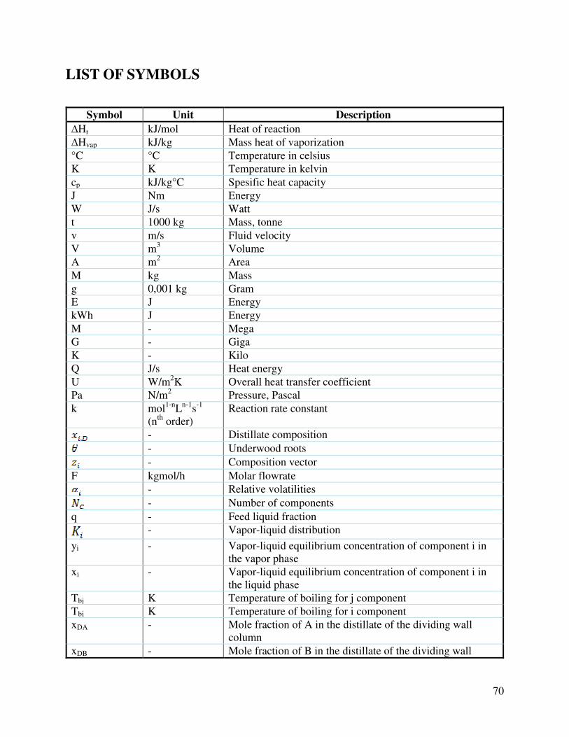
70
LIST OF SYMBOLS
Symbol Unit Description
∆Hr kJ/mol Heat of reaction
∆Hvap kJ/kg Mass heat of vaporization
°C °C Temperature in celsius
K K Temperature in kelvin
cp kJ/kg°C Spesific heat capacity
J Nm Energy
W J/s Watt
t 1000 kg Mass, tonne
v m/s Fluid velocity
V m3 Volume
A m2 Area
M kg Mass
g 0,001 kg Gram
E J Energy
kWh J Energy
M - Mega
G - Giga
K - Kilo
Q J/s Heat energy
U W/m2K Overall heat transfer coefficient
Pa N/m2 Pressure, Pascal
k mol1-nLn-1s-1
(nth order) Reaction rate constant
- Distillate composition
- Underwood roots
- Composition vector
F kgmol/h Molar flowrate
- Relative volatilities
- Number of components
q - Feed liquid fraction
- Vapor-liquid distribution
yi - Vapor-liquid equilibrium concentration of component i in the vapor phase
xi - Vapor-liquid equilibrium concentration of component i in the liquid phase
Tbj K Temperature of boiling for j component
Tbi K Temperature of boiling for i component
xDA - Mole fraction of A in the distillate of the dividing wall column
xDB - Mole fraction of B in the distillate of the dividing wall

71
column
xMA - Mole fraction of A in the sidestream of the dividing wall column
xMB - Mole fraction of B in the sidestream of the dividing wall column
xMC - Mole fraction of C in the sidestream of the dividing wall column
xBB - Mole fraction of B in the bottoms of the dividing wall column
xBC - Mole fraction of C in the bottoms of the dividing wall column
dA - Flow rate of A in the distillate of the dividing wall column
dB - Flow rate of B in the distillate of the dividing wall column
mA - Flow rate of A in the sidestream of the dividing wall column
mB - Flow rate of B in the sidestream of the dividing wall Column
mC - Flow rate of C in the sidestream of the dividing wall column
bB - Flow rate of B in the bottoms of the dividing wall column
bC - Flow rate of C in the bottoms of the dividing wall column
fA - Flow rate of A in the feed to the dividing wall column
fB - Flow rate of B in the feed to the dividing wall column
fC - Flow rate of C in the feed to the dividing wall column
Ni;min - Minimum number of allowable stages for column i
Ni - Number of stages for column i
ni - Number of stages above the feed stage of column i
pi - Number of stages below the feed stage of column i
Vi - Vapour flow rate in the rectifying section of column i
Vi - Vapour flow rate in the stripping section of column i
Li - Liquid flow rate in the rectifying section of column i
Li - Liquid flowrate in the stripping section of column i
q - Quality (saturated liquid fraction) of feed to the prefractionator
qi - Quality (saturated liquid fraction) of feed to the column i
Di - Total distillate flow rate from column i
Bi - Total bottoms flow rate from column i
Ri;min - Minimum reflux ratio for column i
Ri - Reflux ratio for column i
αA - Relative volatility of A with respect to C
αB - Relative volatility of B with respect to C
αC - Relative volatility of C with respect to C
d1A - Flow rate of A in the distillate of column i
d1B - Flow rate of B in the distillate of column i
d1C - Flow rate of C in the distillate of column i

72
b1A - Flow rate of A in the bottoms of column i
b1B - Flow rate of B in the bottoms of column i
b1C - Flow rate of C in the bottoms of column i
F - Feed to the prefractionator
F2 - Feed to column 2
F3 - Feed to column 3
M - Sidestream flow rate
d1C;Underwood - Flow rate of C in the distillate of 1 at minimum reflux (given d1A, d1B)
d1C;Fenske - Flow rate of C in the distillate of 1 at infinite reflux (given d1A,d1B)
d1C - Flow rate of C in the distillate of 1 at reflux ratio (given d1A, d1B)
Xi - Reflux factor of the Gilliland correlation for column i
Yi - Plate factor of the Gilliland correlation for column i
Ntotal - Total number of plates of the dividing wall column
Si - Boilup ratio of column i

73
REFERENCES
Argus NGL Americans Methodology from
http://web04.us.argusmedia.com/ArgusStaticContent//Meth/NGL%20AmericasMeth_Latest.pdf
Christiansen A, Skogestad S. and Lien K. ``Complex Distillation Arrangements: Extending the
Petlyuk ideas'', Computers and Chem. Engng., 21, Suppl., S237-S242 (1997). (Supplement from
symposium PSE-97/ESCAPE-7, Trondheim, Norway, 25-29 May 1997)
Christiansen A.C., Skogestad S. and Lien K, ``Partitioned Petlyuk arrangements for quaternary
separations'', Proc. symposium Distillation and Absorbtion 97 (R. Darton, Ed.), 745-756,
Maastricht, Netherlands, 8-10 Sept. 1997. Published by IChemE, UK.
CME 2010 prices from http://www.cmegroup.com/trading/energy/petrochemicals/mont-belvieu-
iso-butane-5-decimal-opis-swap-futures_quotes_settlements_futures.html
Depriester C.L., Chemical Eng. Progr. Symposium Ser., 49 (7), 1 (1953).
Engelien H.K. and Skogestad S. Minimum Energy Diagrams for Multieffect Distillation
Arrangements. Published online April 25, 2005 in Wiley InterScience. From
http://onlinelibrary.wiley.com/doi/10.1002/aic.10453/abstract
Fenske, M. R., 1932, Fractionation of straight-run Pennsylvania gasoline, Ind Eng Chem, 24:
482.
Gilliland, E. R., 1940, Optimum feed-plate composition in multicomponent rectification, Ind Eng
Chem, 32: 918.
Halvorsen I. J. and Skogestad S. Distillation Theory, 1999. From
http://www.nt.ntnu.no/users/skoge/publications/1999/DistillationTheory/original/distillationtheor
y.pdf
Halvorsen I. J. and Skogestad S. Minimum Energy Consumption in Multicomponent Distillation:
Part I. The Vmin-diagram for a Two-product Column. 2002. From
http://www.nt.ntnu.no/users//skoge/publications/2003/Distillation_energy_Petlyuk_parts1-
3/Part_2/old/PetlyukVmin_paper.pdf
Halvorsen I. J. and Skogestad S. Minimum Energy Consumption in Multicomponent Distillation:
Part III. The Vmin-diagram for a Two-product Column. 2002. From
http://www.nt.ntnu.no/users//skoge/publications/2003/Distillation_energy_Petlyuk_parts1-
3/Part_2/old/PetlyukVmin_paper.pdf
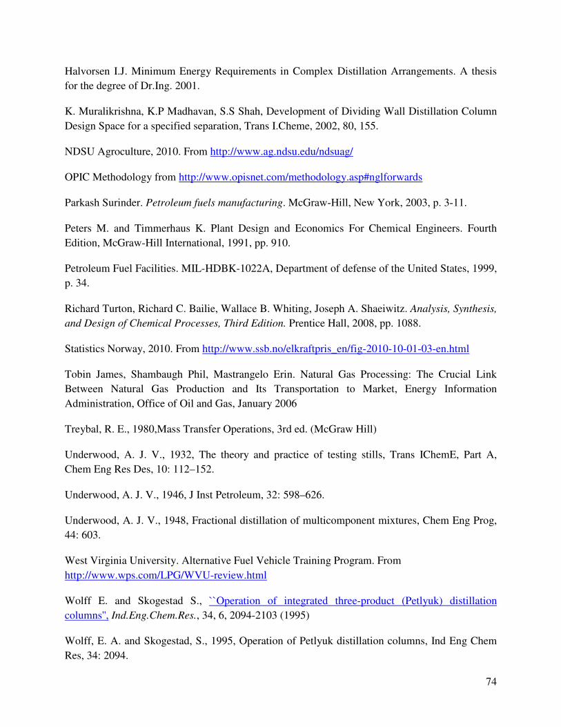
74
Halvorsen I.J. Minimum Energy Requirements in Complex Distillation Arrangements. A thesis
for the degree of Dr.Ing. 2001.
K. Muralikrishna, K.P Madhavan, S.S Shah, Development of Dividing Wall Distillation Column
Design Space for a specified separation, Trans I.Cheme, 2002, 80, 155.
NDSU Agroculture, 2010. From http://www.ag.ndsu.edu/ndsuag/
OPIC Methodology from http://www.opisnet.com/methodology.asp#nglforwards
Parkash Surinder. Petroleum fuels manufacturing. McGraw-Hill, New York, 2003, p. 3-11.
Peters M. and Timmerhaus K. Plant Design and Economics For Chemical Engineers. Fourth
Edition, McGraw-Hill International, 1991, pp. 910.
Petroleum Fuel Facilities. MIL-HDBK-1022A, Department of defense of the United States, 1999,
p. 34.
Richard Turton, Richard C. Bailie, Wallace B. Whiting, Joseph A. Shaeiwitz. Analysis, Synthesis,
and Design of Chemical Processes, Third Edition. Prentice Hall, 2008, pp. 1088.
Statistics Norway, 2010. From http://www.ssb.no/elkraftpris_en/fig-2010-10-01-03-en.html
Tobin James, Shambaugh Phil, Mastrangelo Erin. Natural Gas Processing: The Crucial Link
Between Natural Gas Production and Its Transportation to Market, Energy Information
Administration, Office of Oil and Gas, January 2006
Treybal, R. E., 1980,Mass Transfer Operations, 3rd ed. (McGraw Hill)
Underwood, A. J. V., 1932, The theory and practice of testing stills, Trans IChemE, Part A,
Chem Eng Res Des, 10: 112–152.
Underwood, A. J. V., 1946, J Inst Petroleum, 32: 598–626.
Underwood, A. J. V., 1948, Fractional distillation of multicomponent mixtures, Chem Eng Prog,
44: 603.
West Virginia University. Alternative Fuel Vehicle Training Program. From
http://www.wps.com/LPG/WVU-review.html
Wolff E. and Skogestad S., ``Operation of integrated three-product (Petlyuk) distillation
columns'', Ind.Eng.Chem.Res., 34, 6, 2094-2103 (1995)
Wolff, E. A. and Skogestad, S., 1995, Operation of Petlyuk distillation columns, Ind Eng Chem
Res, 34: 2094.

75
APPENDICES
Appendix A - Computational Procedure for Vmin diagram
>> help UWmulti UWmulti(theta,alfa,zf,qf) [Vs,Ds,Rs,Keys]=UWmulti(theta,alfa,zf,qf) [Vs,Ds,Rs,Keys]=UWmulti(theta,alfa,zf,qf,F) [Vs,Ds,Rs,Keys,theta,VM,h]=UWmulti(theta,alfa,zf,qf,F,inkey,plotflag) [Vs,Ds,Rs,Keys,theta,VM,h]=UWmulti(theta,alfa,zf,qf,F,[],plotflag) [Vs,Ds,Rs,Keys,theta,VM,h]=UWmulti([],alfa,zf,qf,1,[],1) Compute the minimum energy points of the multicomponent-mountains Every set V,D and R is computed as the point of minimum energy comsumption for a legal combination of LK and HK Vs=[V1;V2;...],Ds=[D1; ...],R=[R1;R2....] Keys=[LK1,HK1;LK2,HK2;.....] theta: underwood roots, as from theta=UWroots(alfa,zf,qf) VM : equation matrix h : figure handle(s) from plotting inkey : If included in argument list, compute for Keys==inkeys plotflag: If plotflag==1 or nargout==0, plot the regions Author I. Halvorsen 990417 >> alfa=[13635622.5, 2701765.2, 804757.2, 332796.4, 240499.5, 99990.6, 75918.4, 24888.0, 8474.7, 2900.2, 1039.1, 382.9, 136.1, 56.2, 18.2, 5.6, 2.7, 1] alfa = 1.0e+007 * Columns 1 through 9 1.3636 0.2702 0.0805 0.0333 0.0240 0.0100 0.0076 0.0025 0.0008 Columns 10 through 18 0.0003 0.0001 0.0000 0.0000 0.0000 0.0000 0.0000 0.0000 0.0000 >> zf=[8.66E-02, 4.46E-02, 5.81E-02, 3.16E-02, 5.92E-02, 5.49E-02, 4.96E-02, 8.70E-02, 1.00E-01, 0.1265589, 8.09E-02, 6.14E-02, 5.29E-02, 4.76E-02, 2.08E-02, 1.54E-02, 1.21E-02, 9.38E-03] zf = Columns 1 through 9 0.0866 0.0446 0.0581 0.0316 0.0592 0.0549 0.0496 0.0870 0.1000 Columns 10 through 18 0.1266 0.0809 0.0614 0.0529 0.0476 0.0208 0.0154 0.0121 0.0094 >> qf=0.9987 qf =0.9987

76
>> F=1 F =1 >> plotflag=1 plotflag =1 >> [Vs,Ds,Rs,Keys,theta,VM,h]=UWmulti([],alfa,zf,qf,1,[],1) For five products >> help UWrspec (components) [V,D,R,XT,XB]=UWrspec(VM,zf,LK,HK,LKV,HKV) [V,D,R] =UWrspec(VM,zf,LK,HK,LKV,HKV) [V,D,R] =UWrspec(VM,zf,LK,HK,LKV,HKV,F) Compute operating point as function of two specified component recoveries VM : equation matrix as returned from UWmulti zf : feed composition LK : Light key index HK : Light key index (Note HK>LK) LKV : Specification of light key recovery in rectifying section HKV : Specification of heavy key recovery in rectifying section : Note HK>LK and LKV>HKV V : Overhead vapour flow rate D : Overhead product R : Overhead product recoveries XT : Overhead product composition XB : Bottoms product composition >> LK=2 LK =2 >> HK=3 HK =3 >> LKV=1 LKV =1 >> HKV=0 HKV =0 >> [V,D,R] =UWrspec(VM,zf,LK,HK,LKV,HKV) V =0.1728 D =0.1312 R = Columns 1 through 16 1 1 0 0 0 0 0 0 0 0 0 0 0 0 0 0 Columns 17 through 18
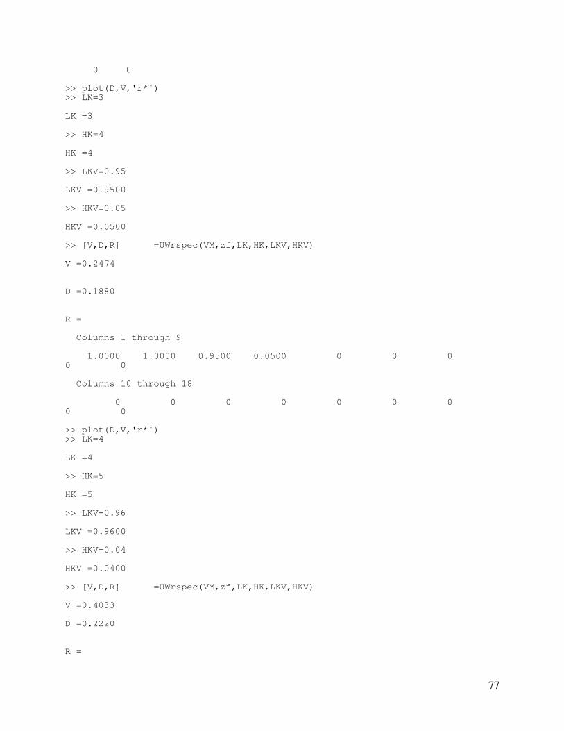
77
0 0 >> plot(D,V,'r*') >> LK=3 LK =3 >> HK=4 HK =4 >> LKV=0.95 LKV =0.9500 >> HKV=0.05 HKV =0.0500 >> [V,D,R] =UWrspec(VM,zf,LK,HK,LKV,HKV) V =0.2474 D =0.1880 R = Columns 1 through 9 1.0000 1.0000 0.9500 0.0500 0 0 0 0 0 Columns 10 through 18 0 0 0 0 0 0 0 0 0 >> plot(D,V,'r*') >> LK=4 LK =4 >> HK=5 HK =5 >> LKV=0.96 LKV =0.9600 >> HKV=0.04 HKV =0.0400 >> [V,D,R] =UWrspec(VM,zf,LK,HK,LKV,HKV) V =0.4033 D =0.2220 R =

78
Columns 1 through 9 1.0000 1.0000 1.0000 0.9600 0.0400 0 0 0 0 Columns 10 through 18 0 0 0 0 0 0 0 0 0 >> plot(D,V,'r*') >> LK=5 LK = 5 >> HK=6 HK =6 >> LKV=1 LKV =1 >> HKV=0 HKV =0 >> [V,D,R] =UWrspec(VM,zf,LK,HK,LKV,HKV) V =0.3720 D =0.2801 R = Columns 1 through 16 1 1 1 1 1 0 0 0 0 0 0 0 0 0 0 0 Columns 17 through 18 0 0 >> plot(D,V,'r*') For four products >> help UWrspec [V,D,R,XT,XB]=UWrspec(VM,zf,LK,HK,LKV,HKV) [V,D,R] =UWrspec(VM,zf,LK,HK,LKV,HKV) [V,D,R] =UWrspec(VM,zf,LK,HK,LKV,HKV,F) Compute operating point as function of two specified component recoveries VM : equation matrix as returned from UWmulti zf : feed composition LK : Light key index HK : Light key index (Note HK>LK) LKV : Specification of light key recovery in rectifying section HKV : Specification of heavy key recovery in rectifying section
79
: Note HK>LK and LKV>HKV V : Overhead vapour flow rate D : Overhead product R : Overhead product recoveries XT : Overhead product composition XB : Bottoms product composition >> LK=2 LK =2 >> HK=3 HK =3 >> LKV=1 LKV =1 >> HKV=0 HKV =0 >> [V,D,R] =UWrspec(VM,zf,LK,HK,LKV,HKV) V =0.1728 D = 0.1312 R = Columns 1 through 16 1 1 0 0 0 0 0 0 0 0 0 0 0 0 0 0 Columns 17 through 18 0 0 >> plot(D,V,'r*') >> LK=3 LK =3 >> HK=4 HK =4 >> LKV=0.95 LKV =0.9500 >> HKV=0.05 HKV =0.0500 >> [V,D,R] =UWrspec(VM,zf,LK,HK,LKV,HKV) V =0.2474

80
D =0.1880 R = Columns 1 through 9 1.0000 1.0000 0.9500 0.0500 0 0 0 0 0 Columns 10 through 18 0 0 0 0 0 0 0 0 0 >> plot(D,V,'r*') >> LK=5 LK =5 >> HK=6 HK =6 >> LKV=0.99 LKV =0.9900 >> HKV=0.01 HKV =0.0100 >> [V,D,R] =UWrspec(VM,zf,LK,HK,LKV,HKV) V =0.3683 D =0.2801 R = Columns 1 through 9 1.0000 1.0000 1.0000 1.0000 0.9900 0.0100 0 0 0 Columns 10 through 18 0 0 0 0 0 0 0 0 0 >> plot(D,V,'r*')
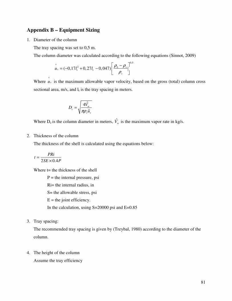
81
Appendix B – Equipment Sizing
1. Diameter of the column
The tray spacing was set to 0,5 m.
The column diameter was calculated according to the following equations (Sinnot, 2009)
0,5^
2( 0,17 0,27 0,047) L vv t t
v
u l lρ ρ
ρ
−= − + −
Where ^
vu is the maximum allowable vapor velocity, based on the gross (total) column cross
sectional area, m/s, and lt is the tray spacing in meters.
ˆ4
ˆw
c
v v
VD
uπρ=
Where Dc is the column diameter in meters, ˆwV is the maximum vapor rate in kg/s.
2. Thickness of the column
The thickness of the shell is calculated using the equations below:
PSE
PRit
4.02 ×=
Where t= the thickness of the shell
P = the internal pressure, psi
Ri= the internal radius, in
S= the allowable stress, psi
E = the joint efficiency.
In the calculation, using S=20000 psi and E=0.85
3. Tray spacing:
The recommended tray spacing is given by (Treybal, 1980) according to the diameter of the
column.
4. The height of the column
Assume the tray efficiency

82
the number of ideal tray
the number of real trayEo = =0.85
The number of real tray=0.85× the number of ideal tray
The height of the column = the number of the real tray × tray spacing
The overall height=1.2× the height of the column, considering the length of the head account for
20% of the overall height.
Table B.1 - Key Data of the Equipment
5. Sizing of condensers and reboilers
Heat transfer coefficients for the fluids used in the model are given in table below.
Table B.2 – Heat Transfer Coefficients (Skogestad, 2003)
Fluids Heat transfer coefficients [W/m2 K]
High pressure process stream - water 570
High pressure process stream - vaporizing water (assumed)
500
High pressure process stream - high pressure vapor
450
High pressure process stream - high pressure process stream
450
Low pressure process stream - water 140
Boiling liquid- condensing vapor 800
Boiling liquid - cooling of super heated steam (assumed)
800
Variable Deethanizer Debutanizer Propane Column
Butane Column
ut [m/s] 0.284 0.141 0.209 0.296
ρL[kg/m3] 678.8 488.6 504.8 539.6
ρv [kg/m3] 16.96 45.98 22.88 12.46
Vv[m/s] 9.17 8.75 0.659 0.476
Dc ,mm 1.55 1.31 0.419 0.405
Shell thickness, mm 8 6.35 6.35 6.35
Tray number 30 47 34 42
Tray spacing,m 0.6 0.6 0.5 0.5
Height,m 21.6 33.84 20.4 25.2

83
The exchanger area was calculated by using the duty given from UniSIM. The log mean
temperature difference was calculated for each reboiler and condenser.
Example:
Duty: Q (given from UniSIM)
t∆ =LMTD (log mean temperature difference) = 1 2
1
2
T T
Tln
T
∆ − ∆
∆
∆
Where, 1T∆ is the temperature difference between the hot inlet stream and cold outlet is stream
and 2T∆ is the difference between the hot outlet stream and the cold inlet stream.
Using the relation:
tK
QA
∆=
The heat exchanger area could then be calculated. The results are shown in Table B.3.
A. Condenser calculation
1. The amount of cooling water needed for the condenser for debutanizer. The sea temperature
used for condense is 10 oC, assume the outlet temperature is 40 oC.
hkgtCp
QG
OH
OH /0.89920)1040(2.4
10133.1 7
2
2 =−×
×=
∆⋅=
03.55
1065.76
4086.84ln
)1065.76()4086.84(
ln
)()(
21
12
2112 =
−
−
−−−=
−
−
−−−=∆
tT
tT
tTtTt ℃
The heat exchanger area:
27
36155570
10133.1m
tK
QA =
×
×=
∆=
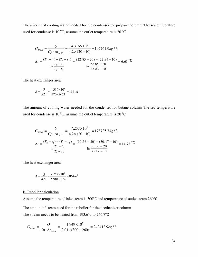
84
The amount of cooling water needed for the condenser for propane column. The sea temperature
used for condense is 10 oC, assume the outlet temperature is 20 oC
hkgtCp
QG
OH
OH /9.102761)1020(2.4
10316.4 6
2
2 =−×
×=
∆⋅=
63.6
1083.22
2085.22ln
)1083.22()2085.22(
ln
)()(
21
12
2112 =
−
−
−−−=
−
−
−−−=∆
tT
tT
tTtTt ℃
The heat exchanger area:
26
114163.6570
10316.4m
tK
QA =
×
×=
∆=
The amount of cooling water needed for the condenser for butane column The sea temperature
used for condense is 10 oC, assume the outlet temperature is 20 oC
hkgtCp
QG
OH
OH /7.178725)1020(2.4
10257.7 6
2
2 =−×
×=
∆⋅=
72.14
1017.30
2036.30ln
)1017.30()2036.30(
ln
)()(
21
12
2112 =
−
−
−−−=
−
−
−−−=∆
tT
tT
tTtTt ℃
The heat exchanger area:
26
86472.14570
10257.7m
tK
QA =
×
×=
∆=
B. Reboiler calculation
Assume the temperature of inlet steam is 300℃ and temperature of outlet steam 260℃ The amount of steam need for the reboiler for the deethanizer column
The stream needs to be heated from 193.6℃ to 246.7℃
hkgtCp
QG
steam
steam /9.242412)260300(01.2
10949.1 7
=−×
×=
∆⋅=
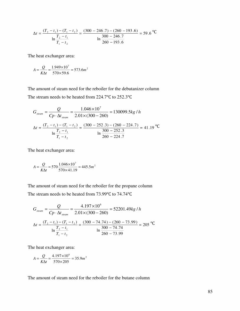
85
6.59
6.193260
7.246300ln
)6.193260()7.246300(
ln
)()(
21
12
2112 =
−
−
−−−=
−
−
−−−=∆
tT
tT
tTtTt ℃
The heat exchanger area:
27
6.5736.59570
10949.1m
tK
QA =
×
×=
∆=
The amount of steam need for the reboiler for the debutanizer column
The stream needs to be heated from 224.7℃ to 252.3℃
hkgtCp
QG
steam
steam /5.130099)260300(01.2
10046.1 7
=−×
×=
∆⋅=
19.41
7.224260
3.252300ln
)7.224260()3.252300(
ln
)()(
21
12
2112 =
−
−
−−−=
−
−
−−−=∆
tT
tT
tTtTt ℃
The heat exchanger area:
27
5.44519.41570
10046.1570 m
tK
QA =
×
×=
∆=
The amount of steam need for the reboiler for the propane column
The stream needs to be heated from 73.99℃ to 74.74℃
hkgtCp
QG
steam
steam /49.52201)260300(01.2
10197.4 6
=−×
×=
∆⋅=
205
99.73260
74.74300ln
)99.73260()74.74300(
ln
)()(
21
12
2112 =
−
−
−−−=
−
−
−−−=∆
tT
tT
tTtTt ℃
The heat exchanger area:
26
9.35205570
10197.4m
tK
QA =
×
×=
∆=
The amount of steam need for the reboiler for the butane column

86
The stream needs to be heated from 50.02℃ to 50.28℃
hkgtCp
QG
steam
steam /19.90261)260300(01.2
10257.7 6
=−×
×=
∆⋅=
229
02.50260
28.50300ln
)02.50260()28.50300(
ln
)()(
21
12
2112 =
−
−
−−−=
−
−
−−−=∆
tT
tT
tTtTt ℃
The heat exchanger area:
26
5.55229570
10257.7m
tK
QA =
×
×=
∆=
Table B.3 – Key Heat Exchanger Data
Description Tag Duty [kW] Surface area [m2] Type
Deethanizer Reboiler E-101 5414 573.6 Kettle
Debutanizer Reboiler E-102 2907 445.5 Kettle
Depropanizer Reboiler E-104 1166 35.9 Kettle
Butane Splitter Reboiler E-106 1976 55.5 Kettle
Debutanizer Condenser E-103 3148 361 Shell and tube
Depropanizer Condenser E-105 1199 1141 Shell and tube
Butane Splitter Condenser E-107 2016 864 Shell and tube

87
Appendix C - Petlyuk Column Calculations
Case 4:
A = C3, B = i-C4 C = n-C4
Table B.4 – Flowrates and Specifications
Component i Relative Volatilities
(αi)
Feed Flowrates (fi, kg mol/hr)
From UNISIM
Distillate Flowrates in column 1 (d1i, kg
mol/hr) Based on Assumed
Recovery
Specifications
A 3.343 14.94 14.92(99% recovery) xD,A=0.9
B 1.383 10.11 5.06(50% recovery) xM,B =0.96
C 1.000 18.84 xB,C =0.94
F= fA + fB + fC = 44.34
= 0.25
Table B.5 – Underwood Roots Calculated Using UWMULTI
Feasible Underwood roots
From equation 12 ɸ1= 2.1834, ɸ2= 1.2068
From equation 29 θ= 1.4930
From equation 34 Ψ = 1.2127
Table B.6 – Calculated Variables
Calculated from Equation Calculated variable
15(b) d1C,Underwood = 0
16 R1,min = 0.7090
17 N1,min = 5.2806
19 d1C,Fenske = 2.8801
20 d1C= 0.9112
21 X1 = 0.3164
22 Y1 = 0.3689
23 N1 = 8.95219=9 24 b1A = 0.1400
25 b1B = 5.0550
26 b1C = 17.9288
27 V1 = 51.9156
28 = 42.8655
32 q2 = -1.5
33 D1 = 20.7662
9 = 65.9893
35 q3 = 2.8537

88
By solving equations (1) to (7)
dA = 14.697
dB = 1.1633
mA = 0.2430
mB = 7.8067
mC = 0.974
bB = 1.1400
bC = 17.8660
38 d3A = 0.1400
39 d3B = 3.9150
40 d3C = 0.0630
36 R2,min = -0.2477
37 R3,min = 6.7028
41 N2,min = 6.9900
42 N3,min = 21.2300
Chosen R2 = 6.0000
46 R3 = 13.3541
21 X2 = 0.8925
22 Y2 = 0.0476
23 N2= 7.3878=8
21 X3 =0 .0616
22 Y3 = 0.5946
23 N3 = 29.5077=30
Table B.7 – Number of Stages in Each Column
Column No. of stages
Prefractionator 9
Column 1 8
Column 2 30
Petlyuk Column Total no. of stages = 47
Case 5:
A = C3, B = i-C4 and n-C4, C = C5+
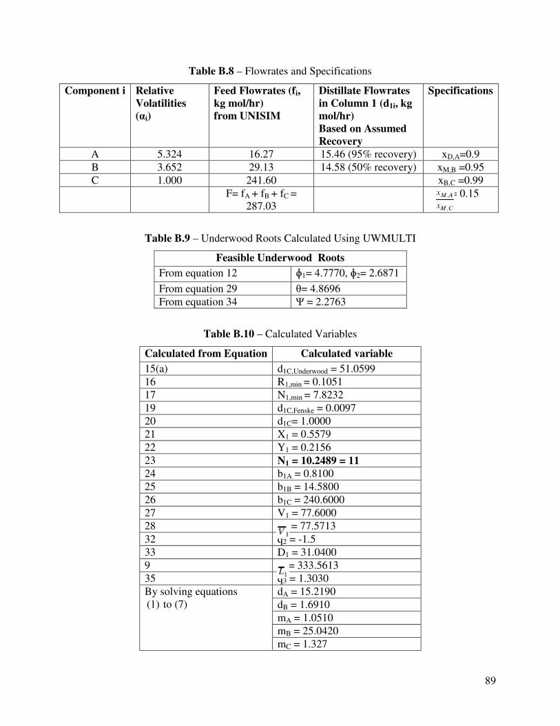
89
Table B.8 – Flowrates and Specifications
Component i Relative Volatilities (αi)
Feed Flowrates (fi, kg mol/hr) from UNISIM
Distillate Flowrates in Column 1 (d1i, kg mol/hr) Based on Assumed Recovery
Specifications
A 5.324 16.27 15.46 (95% recovery) xD,A=0.9
B 3.652 29.13 14.58 (50% recovery) xM,B =0.95
C 1.000 241.60 xB,C =0.99
F= fA + fB + fC = 287.03
= 0.15
Table B.9 – Underwood Roots Calculated Using UWMULTI
Feasible Underwood Roots
From equation 12 ɸ1= 4.7770, ɸ2= 2.6871
From equation 29 θ= 4.8696
From equation 34 Ψ = 2.2763
Table B.10 – Calculated Variables
Calculated from Equation Calculated variable
15(a) d1C,Underwood = 51.0599
16 R1,min = 0.1051
17 N1,min = 7.8232
19 d1C,Fenske = 0.0097
20 d1C= 1.0000
21 X1 = 0.5579
22 Y1 = 0.2156
23 N1 = 10.2489 = 11 24 b1A = 0.8100
25 b1B = 14.5800
26 b1C = 240.6000
27 V1 = 77.6000
28 = 77.5713
32 q2 = -1.5
33 D1 = 31.0400
9 = 333.5613
35 q3 = 1.3030
By solving equations (1) to (7)
dA = 15.2190
dB = 1.6910
mA = 1.0510
mB = 25.0420
mC = 1.327
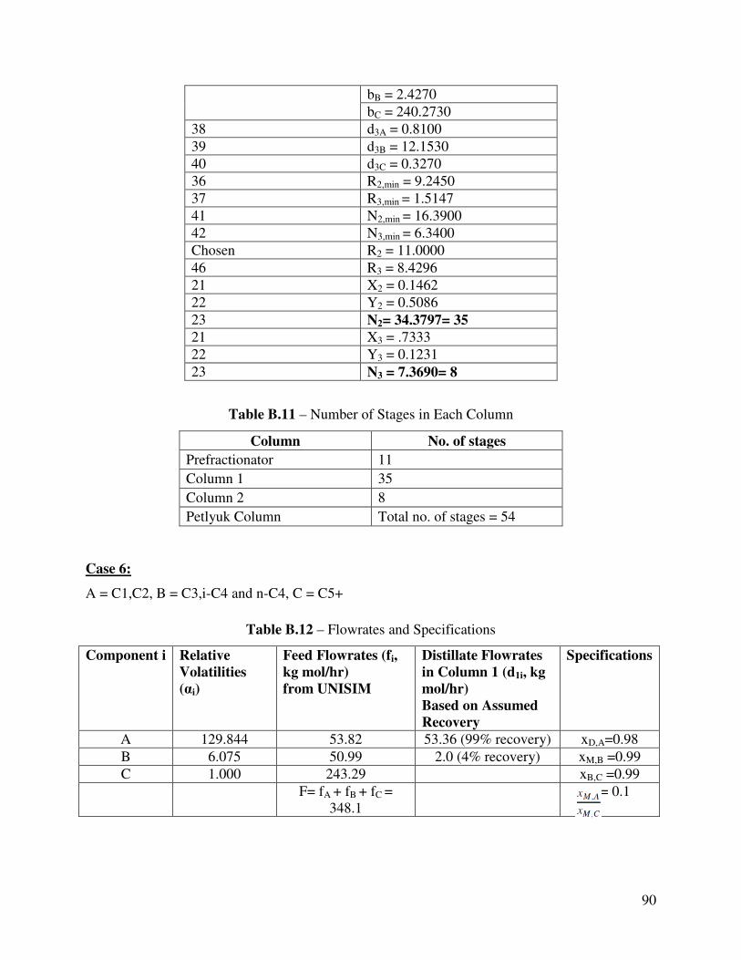
90
bB = 2.4270
bC = 240.2730
38 d3A = 0.8100
39 d3B = 12.1530
40 d3C = 0.3270
36 R2,min = 9.2450
37 R3,min = 1.5147
41 N2,min = 16.3900
42 N3,min = 6.3400
Chosen R2 = 11.0000
46 R3 = 8.4296
21 X2 = 0.1462
22 Y2 = 0.5086
23 N2= 34.3797= 35 21 X3 = .7333
22 Y3 = 0.1231
23 N3 = 7.3690= 8
Table B.11 – Number of Stages in Each Column
Column No. of stages
Prefractionator 11
Column 1 35
Column 2 8
Petlyuk Column Total no. of stages = 54
Case 6:
A = C1,C2, B = C3,i-C4 and n-C4, C = C5+
Table B.12 – Flowrates and Specifications
Component i Relative Volatilities (αi)
Feed Flowrates (fi, kg mol/hr) from UNISIM
Distillate Flowrates in Column 1 (d1i, kg mol/hr) Based on Assumed Recovery
Specifications
A 129.844 53.82 53.36 (99% recovery) xD,A=0.98
B 6.075 50.99 2.0 (4% recovery) xM,B =0.99
C 1.000 243.29 xB,C =0.99
F= fA + fB + fC = 348.1
= 0.1
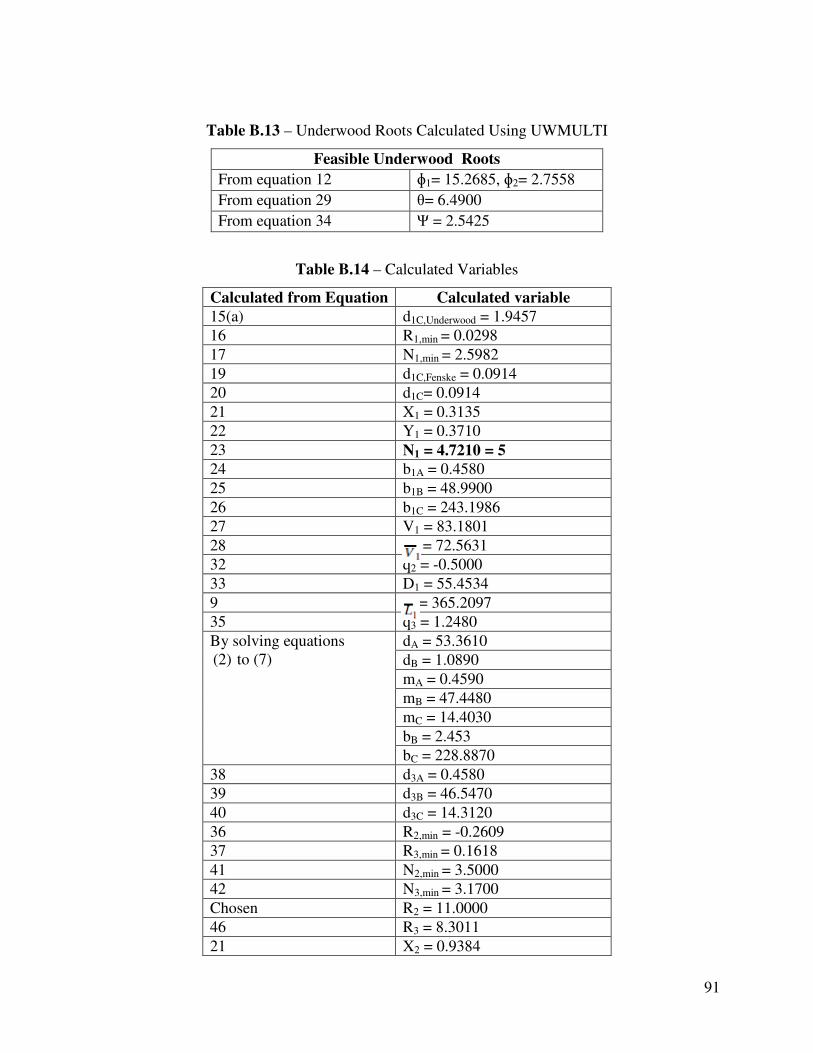
91
Table B.13 – Underwood Roots Calculated Using UWMULTI
Feasible Underwood Roots
From equation 12 ɸ1= 15.2685, ɸ2= 2.7558
From equation 29 θ= 6.4900
From equation 34 Ψ = 2.5425
Table B.14 – Calculated Variables
Calculated from Equation Calculated variable 15(a) d1C,Underwood = 1.9457
16 R1,min = 0.0298
17 N1,min = 2.5982
19 d1C,Fenske = 0.0914
20 d1C= 0.0914
21 X1 = 0.3135
22 Y1 = 0.3710
23 N1 = 4.7210 = 5 24 b1A = 0.4580
25 b1B = 48.9900
26 b1C = 243.1986
27 V1 = 83.1801
28 = 72.5631
32 q2 = -0.5000
33 D1 = 55.4534
9 = 365.2097
35 q3 = 1.2480
By solving equations (2) to (7)
dA = 53.3610
dB = 1.0890
mA = 0.4590
mB = 47.4480
mC = 14.4030
bB = 2.453
bC = 228.8870
38 d3A = 0.4580
39 d3B = 46.5470
40 d3C = 14.3120
36 R2,min = -0.2609
37 R3,min = 0.1618
41 N2,min = 3.5000
42 N3,min = 3.1700
Chosen R2 = 11.0000
46 R3 = 8.3011
21 X2 = 0.9384

92
22 Y2 = 0.0270
23 N2= 3.6209= 4 21 X3 =0.8751
22 Y3 = 0.0555
23 N3 = 3.4129= 4
Table B.15 – Number of Stages in Each Column
Column No. of stages
Prefractionator 5
Column 1 4
Column 2 4
Petlyuk Column Total no. of stages = 13
Figure C.1 - Vmin Diagram for the Third Alternative Petlyuk Column
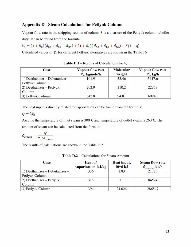
93
Appendix D - Steam Calculations for Petlyuk Column
Vapour flow rate in the stripping section of column 3 is a measure of the Petlyuk column reboiler
duty. It can be found from the formula:
Calculated values of for different Petlyuk alternatives are shown in the Table 16.
Table D.1 – Results of Calculations for
Case Vapour flow rate , kgmole/h
Molecular weight
Vapour flow rate , kg/h
1) Deethanizer – Debutanizer – Petlyuk Column
101.9 53.46 5447.6
2) Deethanizer – Petlyuk Column
202.9 110.2 22359
3) Petlyuk Column 642.8 94.81 60943
The heat input is directly related to vaporization can be found from the formula:
Assume the temperature of inlet steam is 300℃ and temperature of outlet steam is 260℃. The
amount of steam can be calculated from the formula:
The results of calculations are shown in the Table D.2.
Table D.2 – Calculations for Steam Amount
Case Heat of vaporization, kJ/kg
Heat input, 10^6 kJ
Steam flow rate , kg/h
1) Deethanizer – Debutanizer – Petlyuk Column
336 1.83 21785
2) Deethanizer – Petlyuk Column
318 7.1 84524
3) Petlyuk Column 394 24.024 286547

94
Appendix E - Capital Cost Estimation
In this project the estimation of the fixed capital investment was based on the module costing
technique, which is a common technique to estimate the cost of a new chemical plant (Turton,
2003). This costing technique relates all costs back to the purchased cost of equipment evaluated
for some base conditions, which is equipment made of carbon steel and operating at ambient
pressure. Deviations from these base conditions are handled by using multiplying factors that
depends on the following:
• The specific equipment type
• The specific system pressure
• The specific materials of construction
Equation 1 is used to calculate the bare module cost, BM
C , which includes both direct and
indirect cost for each piece of equipment.
0
BM p BMC C F= (1)
where CBM is bare module equipment cost including indirect and direct costs, FBM are the bare
module factor, which is a multiplication factor to account for the direct and indirect cost, as well
as the material of construction and the operating pressure assosiated with the equipment. C0p are
the purchased cost for the base conditions, which is equipment made of carbon steel operating at
ambient pressure.
Purchased equipment cost
Data for the purchased equipment cost of, at ambient operating pressure and using carbon steel
construction are given by the parameter, Cp0, were calculated by the following equation given by
Turton (Turton, 2003):
0 2
1 2 3log log( ) [log( )]pC K K A K A= + + (2)

95
where A is the capacity or size parameter for the equipment. Values for the parameters K1, K2 and
K3, depends on the equipment type.
Pressure factors
As the pressure at which a piece of equipment operates increase, the thickness of the walls of the
equipment will also increase.
Process vessels
To calculate the pressure factors for process vessels and distillation towers the following equation
given by Turton was used:
,
( 1)0,00315
2[850 0,6( 1)]
0,0063P vessel
P D
PF
++
− += for
vesselF >0.0063m (3)
Where, P is the operating pressure, and D represent the diameter of the vessel.
For ,P vesselF less than 1, then ,P vesselF =1
Other process equipment
The pressure factor for the remaining process equipment, are given by the following equation
(Turton, 2003):
2
1 2 3log log (log )PF C C P C P= + + (4)
Where, the unit for pressure are barg. The constants C1, C2 , and C3 depends on the equipment
type.
Bare module and material factors
The bare module factor also depends on the choice of material of construction. This is accounted
for by a material factor FM. The way the material factor, FM, as well as the pressure factor, FP,
relates to the bare module factor differentiate somewhat according to the equipment.
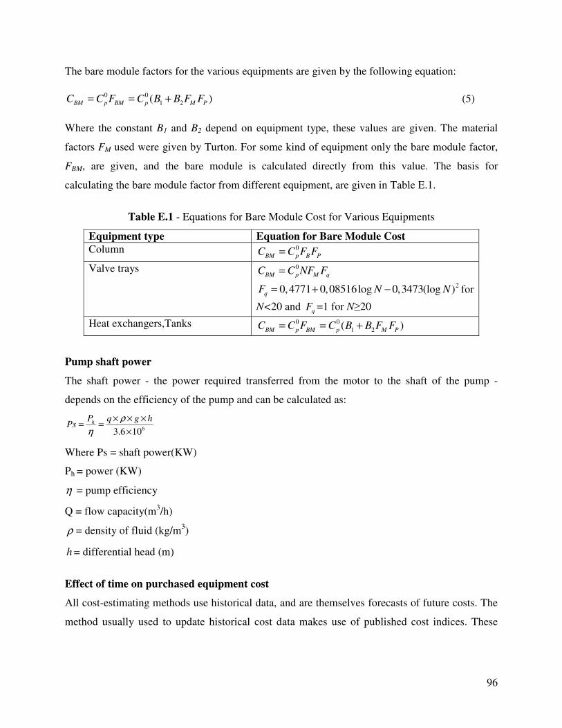
96
The bare module factors for the various equipments are given by the following equation:
0 0
1 2( )BM p BM p M PC C F C B B F F= = + (5)
Where the constant B1 and B2 depend on equipment type, these values are given. The material
factors FM used were given by Turton. For some kind of equipment only the bare module factor,
FBM, are given, and the bare module is calculated directly from this value. The basis for
calculating the bare module factor from different equipment, are given in Table E.1.
Table E.1 - Equations for Bare Module Cost for Various Equipments
Equipment type Equation for Bare Module Cost Column 0
BM p B PC C F F=
Valve trays 0
BM p M qC C NF F=
20,4771 0,08516log 0,3473(log )qF N N= + − for
N<20 and qF =1 for N≥20
Heat exchangers,Tanks 0 0
1 2( )BM p BM p M PC C F C B B F F= = +
Pump shaft power
The shaft power - the power required transferred from the motor to the shaft of the pump -
depends on the efficiency of the pump and can be calculated as:
6106.3 ×
×××==
hgqPPs h ρ
η
Where Ps = shaft power(KW)
Ph = power (KW)
η = pump efficiency
Q = flow capacity(m3/h)
ρ = density of fluid (kg/m3)
h = differential head (m)
Effect of time on purchased equipment cost
All cost-estimating methods use historical data, and are themselves forecasts of future costs. The
method usually used to update historical cost data makes use of published cost indices. These
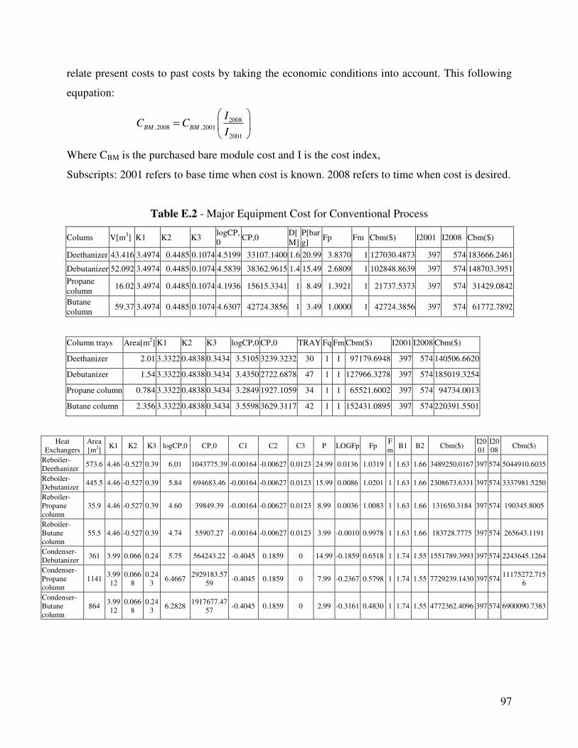
97
relate present costs to past costs by taking the economic conditions into account. This following
equpation:
2008,2008 ,2001
2001
BM BM
IC C
I
=
Where CBM is the purchased bare module cost and I is the cost index,
Subscripts: 2001 refers to base time when cost is known. 2008 refers to time when cost is desired.
Table E.2 - Major Equipment Cost for Conventional Process
Colums V[m3] K1 K2 K3 logCP,0
CP,0 D[M]
P[barg]
Fp Fm Cbm($) I2001 I2008 Cbm($)
Deethanizer 43.416 3.4974 0.4485 0.1074 4.5199 33107.1400 1.6 20.99 3.8370 1 127030.4873 397 574 183666.2461
Debutanizer 52.092 3.4974 0.4485 0.1074 4.5839 38362.9615 1.4 15.49 2.6809 1 102848.8639 397 574 148703.3951
Propane column
16.02 3.4974 0.4485 0.1074 4.1936 15615.3341 1 8.49 1.3921 1 21737.5373 397 574 31429.0842
Butane column
59.37 3.4974 0.4485 0.1074 4.6307 42724.3856 1 3.49 1.0000 1 42724.3856 397 574 61772.7892
Column trays Area[m2] K1 K2 K3 logCP,0 CP,0 TRAY Fq Fm Cbm($) I2001 I2008 Cbm($)
Deethanizer 2.01 3.3322 0.4838 0.3434 3.5105 3239.3232 30 1 1 97179.6948 397 574 140506.6620
Debutanizer 1.54 3.3322 0.4838 0.3434 3.4350 2722.6878 47 1 1 127966.3278 397 574 185019.3254
Propane column 0.784 3.3322 0.4838 0.3434 3.2849 1927.1059 34 1 1 65521.6002 397 574 94734.0013
Butane column 2.356 3.3322 0.4838 0.3434 3.5598 3629.3117 42 1 1 152431.0895 397 574 220391.5501
Heat Exchangers
Area [m2]
K1 K2 K3 logCP,0 CP,0 C1 C2 C3 P LOGFp Fp Fm
B1 B2 Cbm($) I2001
I2008
Cbm($)
Reboiler-Deethanizer
573.6 4.46 -0.527 0.39 6.01 1043775.39 -0.00164 -0.00627 0.0123 24.99 0.0136 1.0319 1 1.63 1.66 3489250.0167 397 574 5044910.6035
Reboiler-Debutanizer
445.5 4.46 -0.527 0.39 5.84 694683.46 -0.00164 -0.00627 0.0123 15.99 0.0086 1.0201 1 1.63 1.66 2308673.6331 397 574 3337981.5250
Reboiler-Propane column
35.9 4.46 -0.527 0.39 4.60 39849.39 -0.00164 -0.00627 0.0123 8.99 0.0036 1.0083 1 1.63 1.66 131650.3184 397 574 190345.8005
Reboiler-Butane column
55.5 4.46 -0.527 0.39 4.74 55907.27 -0.00164 -0.00627 0.0123 3.99 -0.0010 0.9978 1 1.63 1.66 183728.7775 397 574 265643.1191
Condenser-Debutanizer
361 3.99 0.066 0.24 5.75 564243.22 -0.4045 0.1859 0 14.99 -0.1859 0.6518 1 1.74 1.55 1551789.3993 397 574 2243645.1264
Condenser-Propane column
1141 3.9912
0.0668
0.243
6.4667 2929183.57
59 -0.4045 0.1859 0 7.99 -0.2367 0.5798 1 1.74 1.55 7729239.1430 397 574
11175272.7156
Condenser-Butane column
864 3.9912
0.0668
0.243
6.2828 1917677.47
57 -0.4045 0.1859 0 2.99 -0.3161 0.4830 1 1.74 1.55 4772362.4096 397 574 6900090.7383
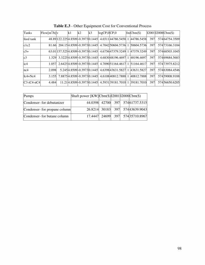
98
Table E.3 - Other Equipment Cost for Conventional Process
Tanks Flow[m3/h] v k1 k2 k3 logCP,0 CP,0 fm Cbm($) I2001 I2008 Cbm($)
feed tank 48.89 122.225 4.8509 -0.3973 0.1445 4.6511 44786.5458 1 44786.5458 397 574 64754.3509
c1c2 81.66 204.15 4.8509 -0.3973 0.1445 4.7042 50604.5736 1 50604.5736 397 574 73166.3104
c5+ 63.01 157.525 4.8509 -0.3973 0.1445 4.6756 47379.3249 1 47379.3249 397 574 68503.1045
c3 1.329 3.3225 4.8509 -0.3973 0.1445 4.6830 48196.4697 1 48196.4697 397 574 69684.5683
ic4 1.057 2.6425 4.8509 -0.3973 0.1445 4.7090 51164.4617 1 51164.4617 397 574 73975.8212
nc4 2.098 5.245 4.8509 -0.3973 0.1445 4.6398 43631.5827 1 43631.5827 397 574 63084.4546
Ic4+Nc4 3.155 7.8875 4.8509 -0.3973 0.1445 4.6108 40812.7888 1 40812.7888 397 574 59008.9188
C3-iC4-nC4 4.484 11.21 4.8509 -0.3973 0.1445 4.5931 39181.7010 1 39181.7010 397 574 56650.6205
Pumps Shaft power [KW] Cbm($) I2001 I2008 Cbm($)
Condenser- for debutanizer 44.0398 42700 397 574 61737.5315
Condenser- for propane column 26.8214 30183 397 574 43639.9043
Condenser- for butane column 17.4447 24699 397 574 35710.8967

99
Appendix F – Cash Flows for Different Alternatives
Table F.1 – Cash Flows for Conventional and Petlyuk Cases
Years Conventional Columns Petlyuk Column Case 1, M$ Case 2, M$ Case 3, M$ Case 1, M$ Case 2, M$ Case 3, M$
0 -159.397 -120.143 -59,886 -3,9041 -58,008 -46,594
1 -63,383 -19,0654 12,3394 -3,9041 17,741176 28,10026
2 -63,383 -19,0654 12,3394 -3,9041 17,741176 28,10026
3 -63,383 -19,0654 12,3394 -3,9041 17,741176 28,10026
4 -63,383 -19,0654 12,3394 -3,9041 17,741176 28,10026
5 -63,383 -19,0654 12,3394 -3,9041 17,741176 28,10026
6 -63,383 -19,0654 12,3394 -3,9041 17,741176 28,10026
7 -63,383 -19,0654 12,3394 -3,9041 17,741176 28,10026
8 -63,383 -19,0654 12,3394 -3,9041 17,741176 28,10026
9 -63,383 -19,0654 12,3394 -3,9041 17,741176 28,10026
10 -63,383 -19,0654 12,3394 -3,9041 17,741176 28,10026
11 -63,383 -19,0654 18,328 -3,9041 21,337672 30,989088
12 -63,383 -19,0654 18,328 -3,9041 21,337672 30,989088
13 -63,383 -19,0654 18,328 -3,9041 21,337672 30,989088
14 -63,383 -19,0654 18,328 -3,9041 21,337672 30,989088
15 -63,383 -19,0654 18,328 -3,9041 21,337672 30,989088
16 -63,383 -19,0654 18,328 -3,9041 21,337672 30,989088
17 -63,383 -19,0654 18,328 -3,9041 21,337672 30,989088
18 -63,383 -19,0654 18,328 -3,9041 21,337672 30,989088
19 -63,383 -19,0654 18,328 -3,9041 21,337672 30,989088
20 -63,383 -19,0654 18,328 -3,9041 21,337672 30,989088
Related Documents