1 Chapter 8 Linear programming is used to allocate resources, plan production, schedule workers, plan investment portfolios and formulate marketing (and military) strategies. The versatility and economic impact of linear programming in today’s industrial world is truly awesome.--Eugene Lawler Linear Programming

Welcome message from author
This document is posted to help you gain knowledge. Please leave a comment to let me know what you think about it! Share it to your friends and learn new things together.
Transcript

1
Chapter 8
Linear programming is used to allocate resources, plan production, schedule workers, plan investment portfolios and formulate marketing (and military) strategies. The versatility and economic impact of linear programming in today’s industrial world is truly awesome.--Eugene Lawler
Linear Programming

2
What is a Linear Program? A linear program is a mathematical model that indicates the goal and requirements of an allocation problem. It has two or more non-negative variables. Its objective is expressed as a mathematical function. The objective function plots as a line on a two-dimensional graph. There are constraints that affect possible levels of the variables. In two dimensions these plot as lines and ordinarily define areas in which the solution must lie.

3
Redwood FurnitureProblem Formulation
Let XT and XC denote the number of tables and chairs to be made. (Define variables)
Maximize P = 6XT + 8XC (Objective function)
Subject to: (Constraints)
30XT + 20XC < 300 (wood)
5XT + 10XC < 110 (labor)
where XT and XC > 0 (non-negativity conditions)
Letting XT represent the horizontal axis and XC the vertical, the constraints and non-negativity conditions define the feasible solution region.

4
Feasible Solution Region for Redwood Furniture Problem

5
Graphing to Find Feasible Solution Region
For an inequality constraint (with < or >), first plot as a line: 30XT + 20XC = 300.
Get two points. Intercepts are easiest: Set XC = 0, solve for XT for horizontal intercept:
30XT + 20(0) = 300 => XT = 300/30 = 10 Set XT = 0, solve for XC for vertical intercept:
30(0) + 20XC = 300 => XC = 300/20 = 15 Above gets wood line. Do same for labor. Mark valid sides and shade feasible solution
region. Any point there satisfies all constraints and non-negativity conditions.
6
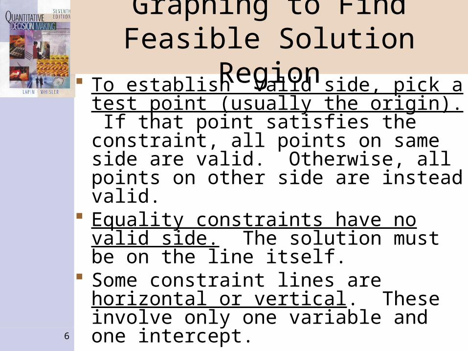
Graphing to Find Feasible Solution Region
To establish valid side, pick a test point (usually the origin). If that point satisfies the constraint, all points on same side are valid. Otherwise, all points on other side are instead valid.
Equality constraints have no valid side. The solution must be on the line itself.
Some constraint lines are horizontal or vertical. These involve only one variable and one intercept.

7
Finding Most Attractive Corner The optimal solution will always correspond to a
corner point of the feasible solution region. Because there can be many corners, the most
attractive corner is easiest to find visually. That is done by plotting two P lines for arbitrary
profit levels. Since the P lines will be parallel, just hold your
pencil at the same angle and role it in from the smaller P’s line toward the bigger one’s That is the direction of improvement.
Continue rolling until only one point lies beneath the pencil. That is the most attractive corner. (Problems can have two most attractive corners.)

8
Most Attractive Corner for Redwood Furniture Problem

9
Finding the Optimal Solution
The coordinates of the most attractive corner provide the optimal levels.
Because reading from graph may be inaccurate, it is best to solve algebraically.
Simultaneously solving the wood and labor equations, the optimal solution is:
XT = 4 tables XC = 9 chairsP = 6(4) + 8(9) = 96 dollars
Note: supply the computed level of the objective in reporting the optimal solution.

10
Advice for Solving Linear Programs
The most attractive corner need not be where the two lines cross. Verify by doubling the table profit. Then the P lines will
be steeper, and (XT = 10, XC = 0) would be best. doubling instead the chair profit. The P lines
will be flatter, and (XT = 0, XC = 11) is best. Problems can have more than 2 constraints. The objective function can involve negative
coefficients. Therefore, the better Ps may not lie to the right. Use 2 lines to guarantee getting right direction.
11
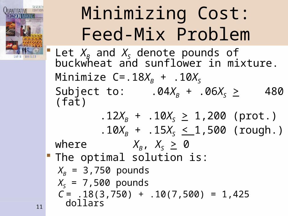
Minimizing Cost:Feed-Mix Problem
Let XB and XS denote pounds of buckwheat and sunflower in mixture.Minimize C=.18XB + .10XS Subject to: .04XB + .06XS > 480 (fat)
.12XB + .10XS > 1,200 (prot.) .10XB + .15XS < 1,500 (rough.)
where XB, XS > 0 The optimal solution is:
XB = 3,750 poundsXS = 7,500 poundsC = .18(3,750) + .10(7,500) = 1,425 dollars
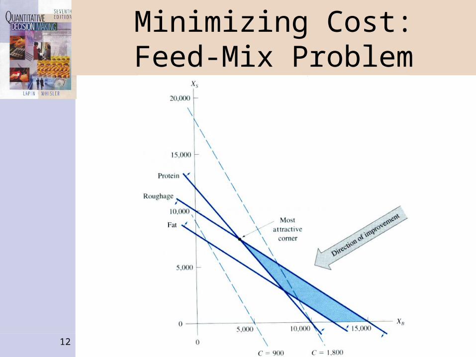
12
Minimizing Cost:Feed-Mix Problem
13
Other Constraint Types
Resources: amount used < available level. Requirements: quan. > minimum (< max.).
XT > 5 (demand) XC < 5 (capacity)
Mixture: product > (or <) multiple of other. XC > 4XT (at least 4 chairs per table made)
XB < .5XS (buckw. not exceed 1/2 wt of sunfl.)
Transform before plotting: XC 4XT > 0 XB .5XS < 0
Equality: XT + XC = 10 (exactly 10 items)
14
Special Problem Types
Infeasible Problems: These arise from contradictions among the constraints. No solution possible until conflict is resolved.
Ties for optimal solution: Multiple optimal solutions can exist. Any linear combination of two optimal corners is also optimal.
Unbounded problems: Feasible solution regions may be open-ended, and the direction of improvement coincides. Mathematically, any profit is possible. Generally nonsensical, possibly due to a
missing constraint. Fix and solve again.

15
Graphing Linear ProgramsUsing Spreadsheets
The Redwood Furniture Company
Maximize P = 6XT + 8XC (objective) Subject to 30XT + 20XC < 300
(wood) 5XT + 10XC < 110
(labor) where XT, XC > 0

16
First StepThe Formulas
The first step is to solve the objective function and each constraint for one of the variables. In this case, solving for XC gives
XC = (P - 6XT)/8 (objective)
XC = (300 - 30XT)/20 (wood)
XC = (110 - 5XT)/10 (labor)
These formulas are entered on the following spreadsheet.
17
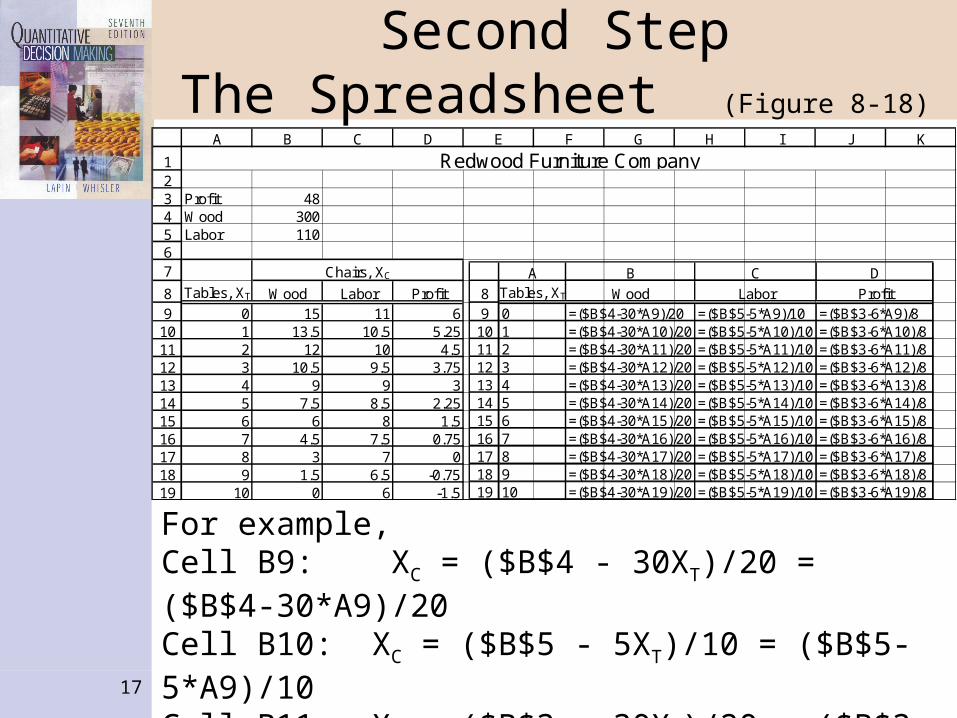
Second StepThe Spreadsheet (Figure 8-18)
1234567
89
10111213141516171819
A B C D E F G H I J K
Profit 48Wood 300Labor 110
Tables, XT Wood Labor Profit0 15 11 61 13.5 10.5 5.252 12 10 4.53 10.5 9.5 3.754 9 9 35 7.5 8.5 2.256 6 8 1.57 4.5 7.5 0.758 3 7 09 1.5 6.5 -0.75
10 0 6 -1.5
Chairs, XC
Redwood Furniture Company
89
10111213141516171819
A B C DTables, XT Wood Labor Profit0 =($B$4-30*A9)/20 =($B$5-5*A9)/10 =($B$3-6*A9)/81 =($B$4-30*A10)/20 =($B$5-5*A10)/10 =($B$3-6*A10)/82 =($B$4-30*A11)/20 =($B$5-5*A11)/10 =($B$3-6*A11)/83 =($B$4-30*A12)/20 =($B$5-5*A12)/10 =($B$3-6*A12)/84 =($B$4-30*A13)/20 =($B$5-5*A13)/10 =($B$3-6*A13)/85 =($B$4-30*A14)/20 =($B$5-5*A14)/10 =($B$3-6*A14)/86 =($B$4-30*A15)/20 =($B$5-5*A15)/10 =($B$3-6*A15)/87 =($B$4-30*A16)/20 =($B$5-5*A16)/10 =($B$3-6*A16)/88 =($B$4-30*A17)/20 =($B$5-5*A17)/10 =($B$3-6*A17)/89 =($B$4-30*A18)/20 =($B$5-5*A18)/10 =($B$3-6*A18)/810 =($B$4-30*A19)/20 =($B$5-5*A19)/10 =($B$3-6*A19)/8
For example,Cell B9: XC = ($B$4 - 30XT)/20 = ($B$4-30*A9)/20Cell B10: XC = ($B$5 - 5XT)/10 = ($B$5-5*A9)/10Cell B11: XC = ($B$3 - 30XT)/20 = ($B$3-30*A9)/20

18
Third StepGraphing with the Chart Wizard
Highlight cells B8:D19 and click on the
chart icon.
Step 1 - Chart Type
Step 2 - Chart Source Data
Step 3 - Chart Options
Step 4 - Chart Location

19
Chart Wizard Chart Type
Select Line as the Chart type and pick the first Chart sub-type (Line) and click Next.
Select Line as the Chart type and pick the first Chart sub-type (Line) and click Next.

20
Chart WizardSources of Data, Series Tab
Enter the horizontal axis values by clicking on the Series tab and entering the range of numbers to be on the horizontal axis, cells A:9:A19, in the Category (X) axis labels line. Alternately, click in the Category (X) axis labels line and then highlight cells A9:A19. Click Next.
Enter the horizontal axis values by clicking on the Series tab and entering the range of numbers to be on the horizontal axis, cells A:9:A19, in the Category (X) axis labels line. Alternately, click in the Category (X) axis labels line and then highlight cells A9:A19. Click Next.

21
Chart WizardChart Options
In the Chart title line type Redwood Furniture Company, in the Category (X) axis put Tables, T, and in the Value (Y) axis line write Chairs, C. Click Next.
In the Chart title line type Redwood Furniture Company, in the Category (X) axis put Tables, T, and in the Value (Y) axis line write Chairs, C. Click Next.

22
Chart WizardChart Location
Click on Finish and the Chart shown next appears.Click on Finish and the Chart shown next appears.

23
Step FourThe Final Graph (Figure 8-19)
Redwood Furniture Company(P = 48)
-4
-2
0
2
4
6
8
10
12
14
16
0 1 2 3 4 5 6 7 8 9 10
Tables, XT
Ch
air
s, X
C
Wood
Labor
Profit
The final graph (after making formatting changes).
The final graph (after making formatting changes).
24
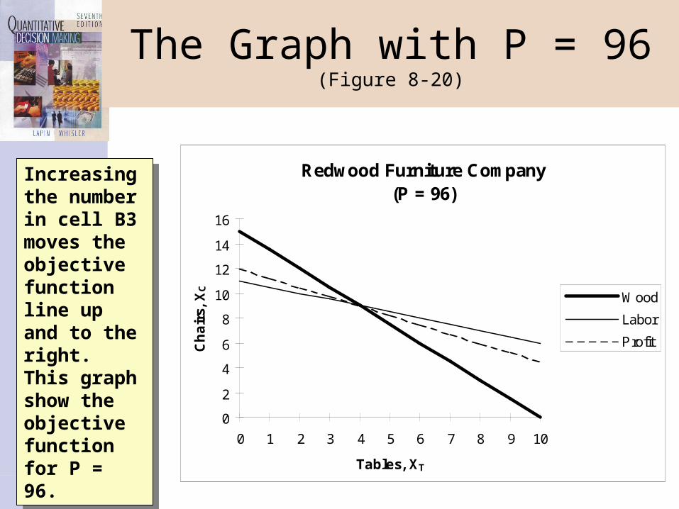
The Graph with P = 96(Figure 8-20)
Redwood Furniture Company(P = 96)
0
2
4
6
8
10
12
14
16
0 1 2 3 4 5 6 7 8 9 10
Tables, XT
Ch
air
s, X
C
Wood
Labor
Profit
Increasing the number in cell B3 moves the objective function line up and to the right. This graph show the objective function for P = 96.
Increasing the number in cell B3 moves the objective function line up and to the right. This graph show the objective function for P = 96.

25
The Graph with P = 96 and 80 Hours of Labor (Figure 8-21)
Redwood Furniture Company(P = 96 and 80 hours of labor)
0
2
4
6
8
10
12
14
16
0 1 2 3 4 5 6 7 8 9 10
Tables, XT
Ch
air
s, X
C
Wood
Labor
Profit
To see what happens when the amount of wood or labor vary, change the numbers in cells B4 (for wood) or B5 (for labor) and the corresponding line will move. This graph show the result when 80 is entered in cell B5 (and P = 96).
To see what happens when the amount of wood or labor vary, change the numbers in cells B4 (for wood) or B5 (for labor) and the corresponding line will move. This graph show the result when 80 is entered in cell B5 (and P = 96).

26
Drawing Horizontaland Vertical Lines
Drawing two types of lines with Excel require special attention: horizontal and vertical lines. The constraint Y = 3 is a horizontal line and the constraint X = 7 is a vertical line. Figure 9-21 shows what an Excel spreadsheet looks like for these two constraints.

27
Spreadsheet forHorizontal and Vertical Lines (Figure 8-22)
123456789
101112131415
A B C D E F
X Y = 3 X = 7 0 3 1000001 3 857142 3 714293 3 571434 3 428575 3 285716 3 142867 3 08 3 -142869 3 -2857110 3 -42857
Graphing Horizontal and Vertical Lines
456789
1011121314
C=100000-(100000/7)*A4=100000-(100000/7)*A5=100000-(100000/7)*A6=100000-(100000/7)*A7=100000-(100000/7)*A8=100000-(100000/7)*A9=100000-(100000/7)*A10=100000-(100000/7)*A11=100000-(100000/7)*A12=100000-(100000/7)*A13=100000-(100000/7)*A14
Vertical Line Equation: Y = 100,000 – (100,000/7)X
The vertical line equation has an Y-intercept of 100,000 and a slope of -(100,000/7). Thus, it is not exactly vertical but it is sufficiently close to vertical for our purposes.
The vertical line equation has an Y-intercept of 100,000 and a slope of -(100,000/7). Thus, it is not exactly vertical but it is sufficiently close to vertical for our purposes.

28
Graphing Horizonaland Vertical Lines (Figure 8-23)
Plotting Horizontal andVertical Lines
0
2
4
6
8
10
0 2 4 6 8 10X
YY = 3
X = 7
To change the position of the vertical line, change the 7 in the denominator of all the formulas in column C to the desired number.
To change the position of the vertical line, change the 7 in the denominator of all the formulas in column C to the desired number.
Related Documents