LP formulations for sparse polynomial optimization problems Daniel Bienstock and Gonzalo Mu˜ noz, Columbia University

Welcome message from author
This document is posted to help you gain knowledge. Please leave a comment to let me know what you think about it! Share it to your friends and learn new things together.
Transcript

LP formulations for sparse polynomialoptimization problems
Daniel Bienstock and Gonzalo Munoz, Columbia University
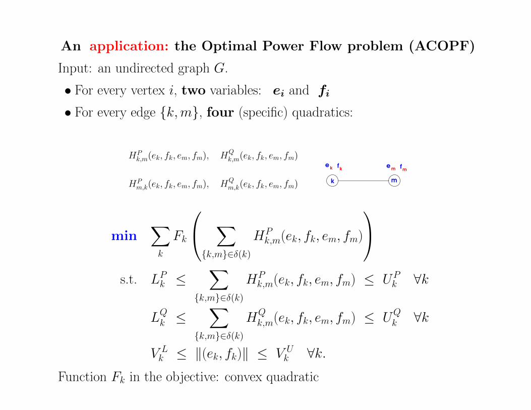
An application: the Optimal Power Flow problem (ACOPF)
Input: an undirected graph G.
• For every vertex i, two variables: ei and fi
• For every edge {k,m}, four (specific) quadratics:
HPk,m(ek, fk, em, fm), HQ
k,m(ek, fk, em, fm)
HPm,k(ek, fk, em, fm), HQ
m,k(ek, fk, em, fm)k m
e efk k m mf
min∑k
Fk
∑{k,m}∈δ(k)
HPk,m(ek, fk, em, fm)
s.t. LPk ≤
∑{k,m}∈δ(k)
HPk,m(ek, fk, em, fm) ≤ UP
k ∀k
LQk ≤∑
{k,m}∈δ(k)
HQk,m(ek, fk, em, fm) ≤ UQ
k ∀k
V Lk ≤ ‖(ek, fk)‖ ≤ V U
k ∀k.Function Fk in the objective: convex quadratic

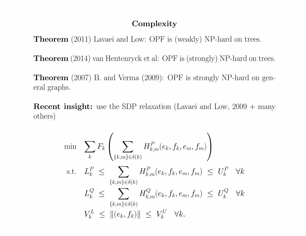
Complexity
Theorem (2011) Lavaei and Low: OPF is (weakly) NP-hard on trees.
Theorem (2014) van Hentenryck et al: OPF is (strongly) NP-hard on trees.
Theorem (2007) B. and Verma (2009): OPF is strongly NP-hard on gen-eral graphs.
Complexity
Theorem (2011) Lavaei and Low: OPF is (weakly) NP-hard on trees.
Theorem (2014) van Hentenryck et al: OPF is (strongly) NP-hard on trees.
Theorem (2007) B. and Verma (2009): OPF is strongly NP-hard on gen-eral graphs.
Recent insight: use the SDP relaxation (Lavaei and Low, 2009 + manyothers)
min∑k
Fk
∑{k,m}∈δ(k)
HPk,m(ek, fk, em, fm)
s.t. LPk ≤
∑{k,m}∈δ(k)
HPk,m(ek, fk, em, fm) ≤ UP
k ∀k
LQk ≤∑
{k,m}∈δ(k)
HQk,m(ek, fk, em, fm) ≤ UQ
k ∀k
V Lk ≤ ‖(ek, fk)‖ ≤ V U
k ∀k.
Complexity
Theorem (2011) Lavaei and Low: OPF is (weakly) NP-hard on trees.
Theorem (2014) van Hentenryck et al: OPF is (strongly) NP-hard on trees.
Theorem (2007) B. and Verma (2009): OPF is strongly NP-hard on gen-eral graphs.
Recent insight: use the SDP relaxation (Lavaei and Low, 2009 + manyothers)
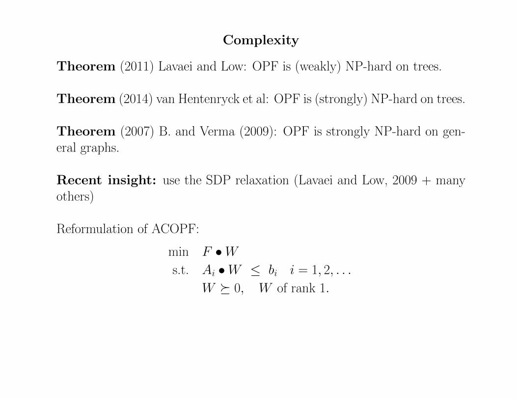
Reformulation of ACOPF:
min F •Ws.t. Ai •W ≤ bi i = 1, 2, . . .
W � 0, W of rank 1.

Complexity
Theorem (2011) Lavaei and Low: OPF is (weakly) NP-hard on trees.
Theorem (2014) van Hentenryck et al: OPF is (strongly) NP-hard on trees.
Theorem (2007) B. and Verma (2009): OPF is strongly NP-hard on gen-eral graphs.
Recent insight: use the SDP relaxation (Lavaei and Low, 2009 + manyothers)
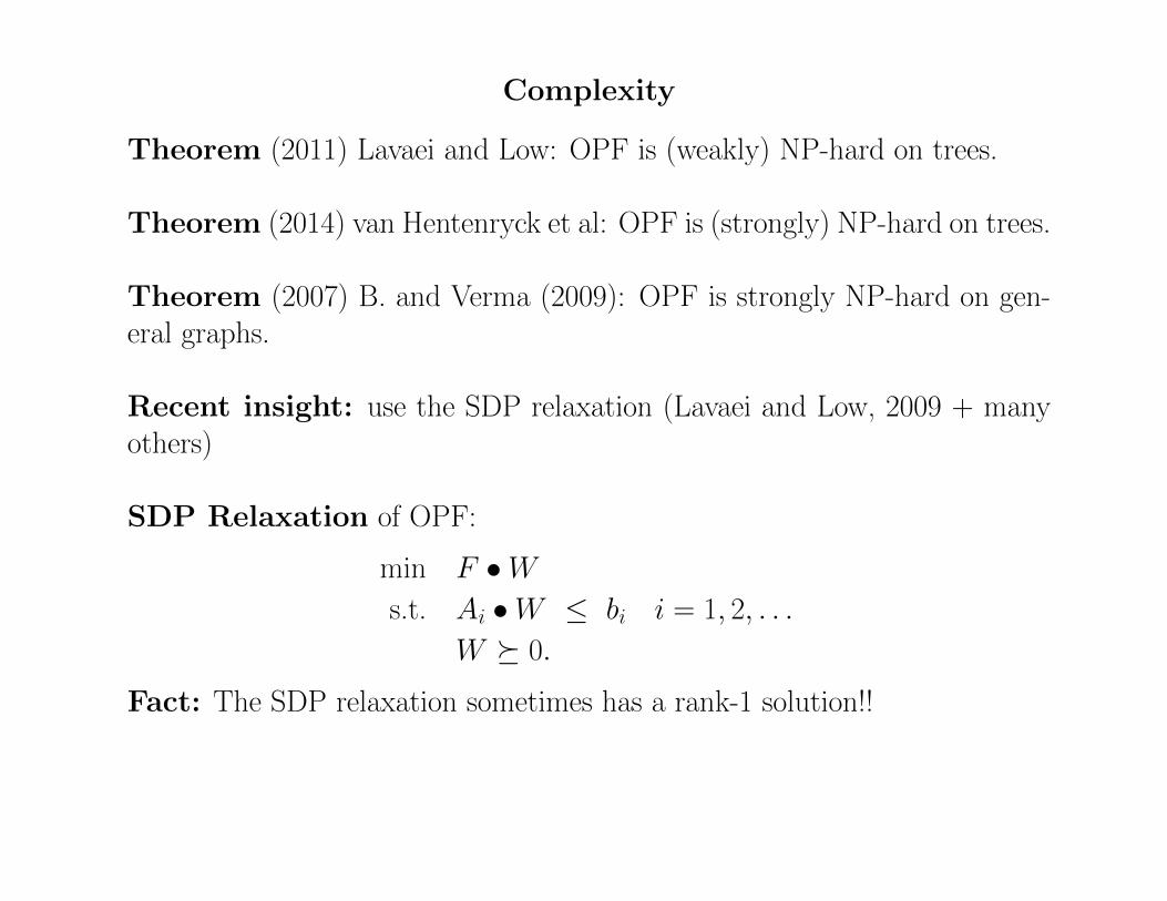
SDP Relaxation of OPF:
min F •Ws.t. Ai •W ≤ bi i = 1, 2, . . .
W � 0.

Complexity
Theorem (2011) Lavaei and Low: OPF is (weakly) NP-hard on trees.
Theorem (2014) van Hentenryck et al: OPF is (strongly) NP-hard on trees.
Theorem (2007) B. and Verma (2009): OPF is strongly NP-hard on gen-eral graphs.
Recent insight: use the SDP relaxation (Lavaei and Low, 2009 + manyothers)
SDP Relaxation of OPF:
min F •Ws.t. Ai •W ≤ bi i = 1, 2, . . .
W � 0.
Fact: The SDP relaxation almost always has a rank-1 solution!!
Complexity
Theorem (2011) Lavaei and Low: OPF is (weakly) NP-hard on trees.
Theorem (2014) van Hentenryck et al: OPF is (strongly) NP-hard on trees.
Theorem (2007) B. and Verma (2009): OPF is strongly NP-hard on gen-eral graphs.
Recent insight: use the SDP relaxation (Lavaei and Low, 2009 + manyothers)
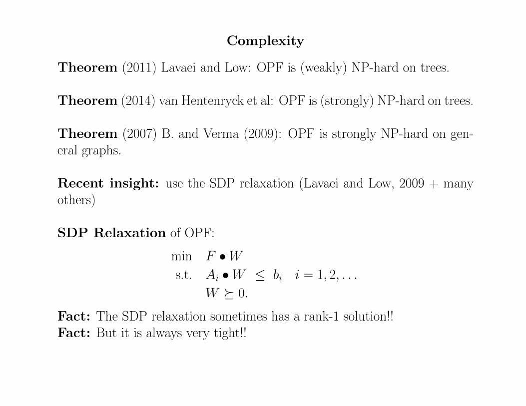
SDP Relaxation of OPF:
min F •Ws.t. Ai •W ≤ bi i = 1, 2, . . .
W � 0.
Fact: The SDP relaxation sometimes has a rank-1 solution!!
Complexity
Theorem (2011) Lavaei and Low: OPF is (weakly) NP-hard on trees.
Theorem (2014) van Hentenryck et al: OPF is (strongly) NP-hard on trees.
Theorem (2007) B. and Verma (2009): OPF is strongly NP-hard on gen-eral graphs.
Recent insight: use the SDP relaxation (Lavaei and Low, 2009 + manyothers)
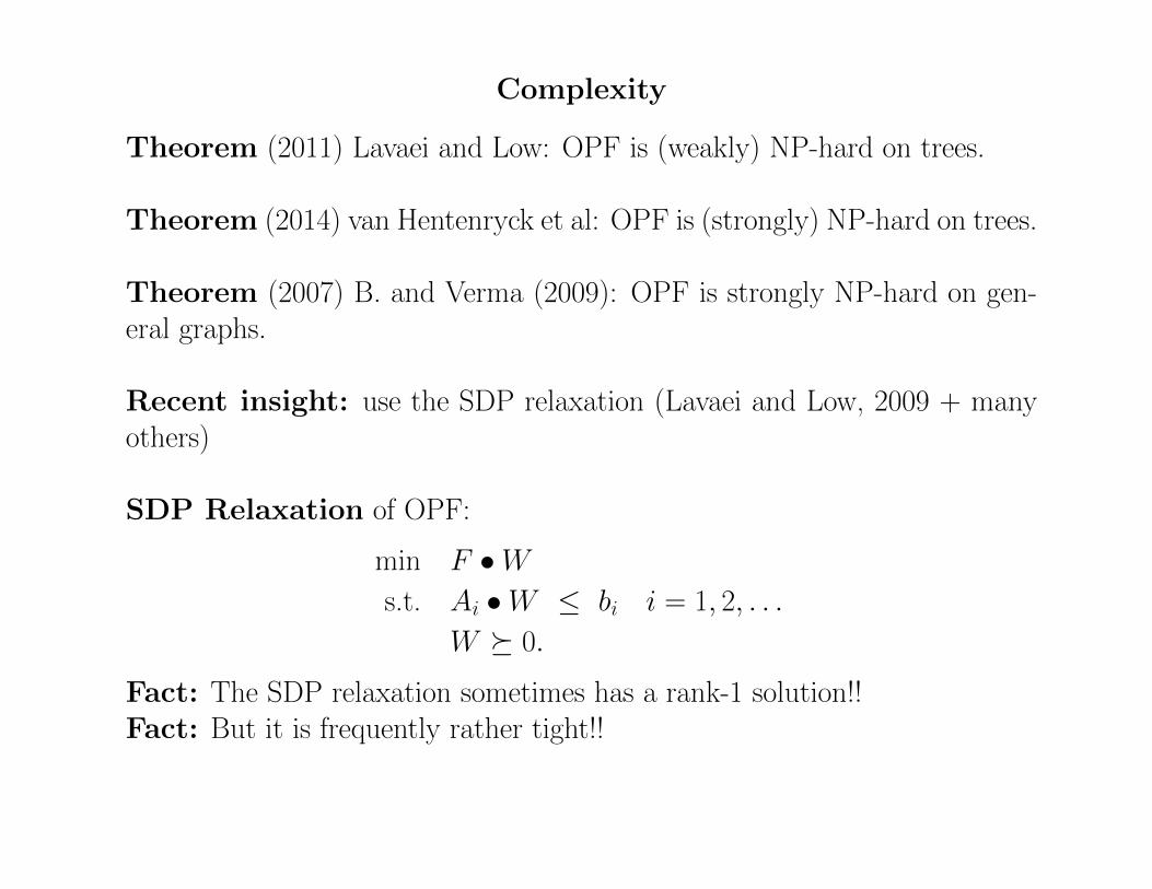
SDP Relaxation of OPF:
min F •Ws.t. Ai •W ≤ bi i = 1, 2, . . .
W � 0.
Fact: The SDP relaxation sometimes has a rank-1 solution!!Fact: But it is always very tight!!
Complexity
Theorem (2011) Lavaei and Low: OPF is (weakly) NP-hard on trees.
Theorem (2014) van Hentenryck et al: OPF is (strongly) NP-hard on trees.
Theorem (2007) B. and Verma (2009): OPF is strongly NP-hard on gen-eral graphs.
Recent insight: use the SDP relaxation (Lavaei and Low, 2009 + manyothers)
SDP Relaxation of OPF:
min F •Ws.t. Ai •W ≤ bi i = 1, 2, . . .
W � 0.
Fact: The SDP relaxation sometimes has a rank-1 solution!!Fact: But it is frequently rather tight!!
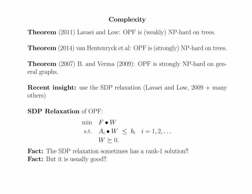
Complexity
Theorem (2011) Lavaei and Low: OPF is (weakly) NP-hard on trees.
Theorem (2014) van Hentenryck et al: OPF is (strongly) NP-hard on trees.
Theorem (2007) B. and Verma (2009): OPF is strongly NP-hard on gen-eral graphs.
Recent insight: use the SDP relaxation (Lavaei and Low, 2009 + manyothers)
SDP Relaxation of OPF:
min F •Ws.t. Ai •W ≤ bi i = 1, 2, . . .
W � 0.
Fact: The SDP relaxation sometimes has a rank-1 solution!!Fact: But it is usually good!!
But: the SDP relaxation is always slow on large graphs
• Real-life grids → > 104 vertices
• SDP relaxation of OPF does not terminate
But...

But: the SDP relaxation is always slow on large graphs
• Real-life grids → > 104 vertices
• SDP relaxation of OPF does not terminate
But...Fact? Real-life grids have small tree-width
Definition 1: A graph has treewidth ≤ w if it has a chordal supergraphwith clique number ≤ w + 1
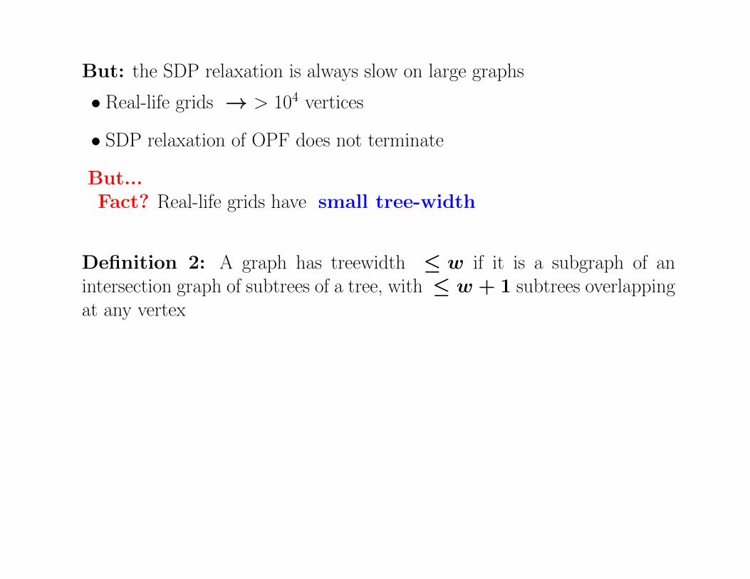
But: the SDP relaxation is always slow on large graphs
• Real-life grids → > 104 vertices
• SDP relaxation of OPF does not terminate
But...Fact? Real-life grids have small tree-width
Definition 2: A graph has treewidth ≤ w if it is a subgraph of anintersection graph of subtrees of a tree, with ≤ w + 1 subtrees overlappingat any vertex
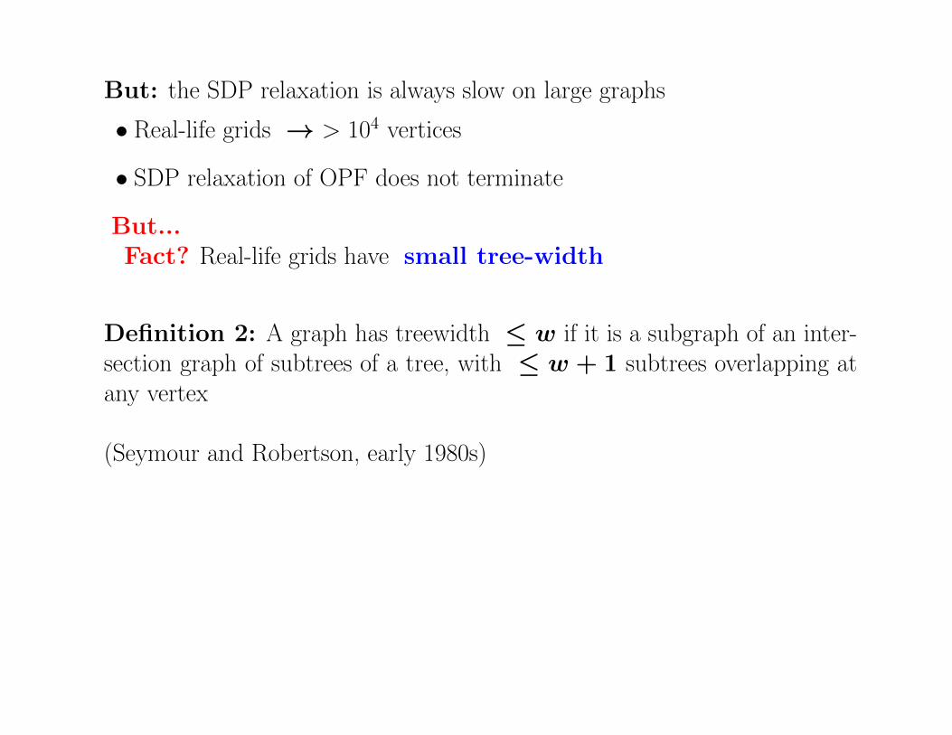
But: the SDP relaxation is always slow on large graphs
• Real-life grids → > 104 vertices
• SDP relaxation of OPF does not terminate
But...Fact? Real-life grids have small tree-width
Definition 2: A graph has treewidth ≤ w if it is a subgraph of an inter-section graph of subtrees of a tree, with ≤ w + 1 subtrees overlapping atany vertex
(Seymour and Robertson, early 1980s)
Tree-width
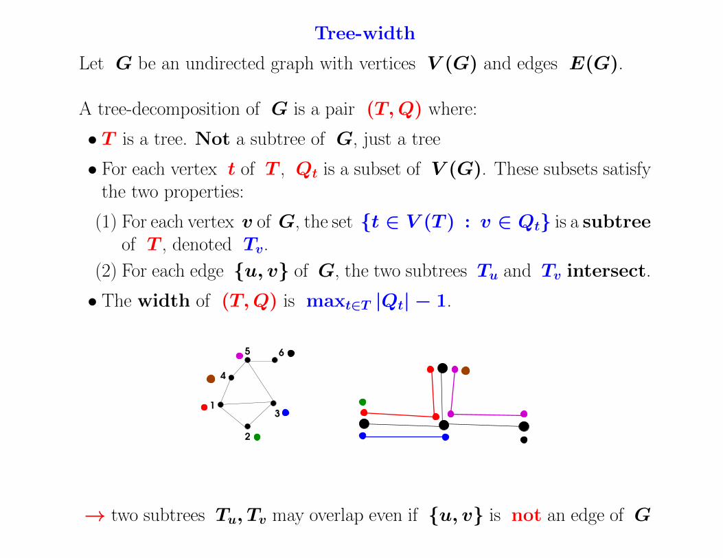
Let G be an undirected graph with vertices V (G) and edges E(G).
A tree-decomposition of G is a pair (T,Q) where:
• T is a tree. Not a subtree of G, just a tree
• For each vertex t of T , Qt is a subset of V (G). These subsets satisfythe two properties:
(1) For each vertex v of G, the set {t ∈ V (T ) : v ∈ Qt} is a subtreeof T , denoted Tv.
(2) For each edge {u, v} of G, the two subtrees Tu and Tv intersect.
• The width of (T,Q) is maxt∈T |Qt| − 1.
1
2
3
4
5 6
→ two subtrees Tu, Tv may overlap even if {u, v} is not an edge of G
Tree-width
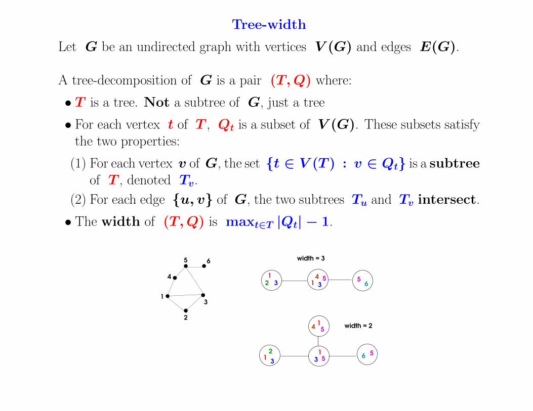
Let G be an undirected graph with vertices V (G) and edges E(G).
A tree-decomposition of G is a pair (T,Q) where:
• T is a tree. Not a subtree of G, just a tree
• For each vertex t of T , Qt is a subset of V (G). These subsets satisfythe two properties:
(1) For each vertex v of G, the set {t ∈ V (T ) : v ∈ Qt} is a subtreeof T , denoted Tv.
(2) For each edge {u, v} of G, the two subtrees Tu and Tv intersect.
• The width of (T,Q) is maxt∈T |Qt| − 1.
width = 3
width = 2
1
2
3
4
5 6
1
2 3 1 3
545
35
54
2 51
1
1 36
6
But: the SDP relaxation is always slow on large graphs
• Real-life grids → > 104 vertices
• SDP relaxation of OPF does not terminate
But...Fact? Real-life grids have small tree-width
Matrix-completion Theorem
gives fast SDP implementations:
Real-life grids with ≈ 3× 10³ vertices: → 20 minutes runtime
→ Perhaps low tree-width yields direct algorithms for ACOPF itself?
That is to say, not for a relaxation?
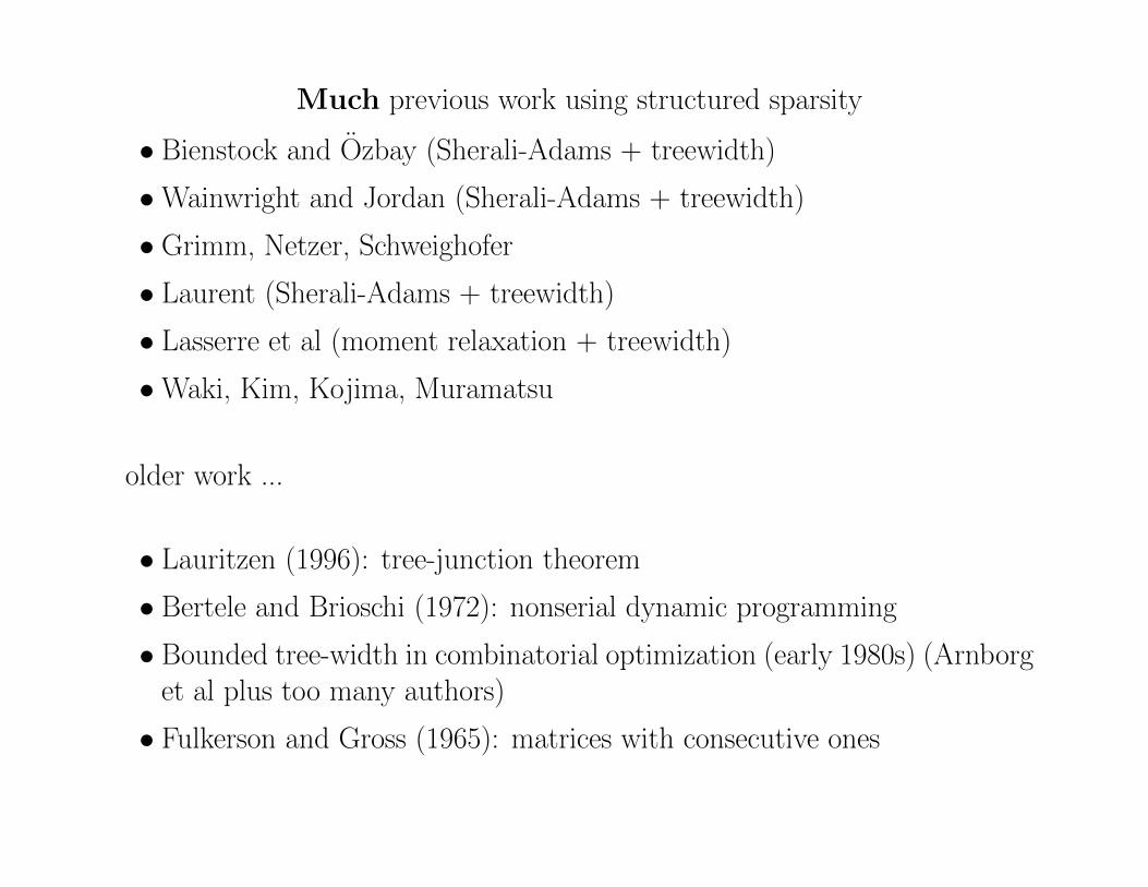
Much previous work using structured sparsity
• Bienstock and Ozbay (Sherali-Adams + treewidth)
•Wainwright and Jordan (Sherali-Adams + treewidth)
• Grimm, Netzer, Schweighofer
• Laurent (Sherali-Adams + treewidth)
• Lasserre et al (moment relaxation + treewidth)
•Waki, Kim, Kojima, Muramatsu
older work ...
• Lauritzen (1996): tree-junction theorem
• Bertele and Brioschi (1972): nonserial dynamic programming
• Bounded tree-width in combinatorial optimization (early 1980s) (Arnborget al plus too many authors)
• Fulkerson and Gross (1965): matrices with consecutive ones
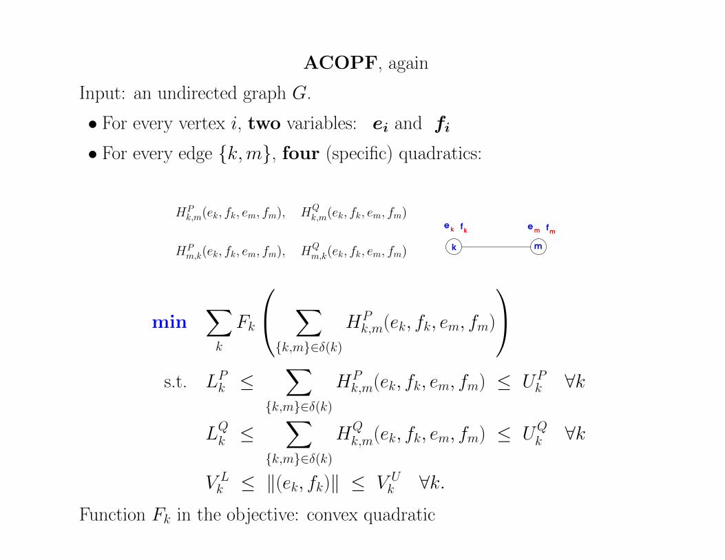
ACOPF, again
Input: an undirected graph G.
• For every vertex i, two variables: ei and fi
• For every edge {k,m}, four (specific) quadratics:
HPk,m(ek, fk, em, fm), HQ
k,m(ek, fk, em, fm)
HPm,k(ek, fk, em, fm), HQ
m,k(ek, fk, em, fm)k m
e efk k m mf
min∑k
Fk
∑{k,m}∈δ(k)
HPk,m(ek, fk, em, fm)
s.t. LPk ≤
∑{k,m}∈δ(k)
HPk,m(ek, fk, em, fm) ≤ UP
k ∀k
LQk ≤∑
{k,m}∈δ(k)
HQk,m(ek, fk, em, fm) ≤ UQ
k ∀k
V Lk ≤ ‖(ek, fk)‖ ≤ V U
k ∀k.Function Fk in the objective: convex quadratic

ACOPF, again
Input: an undirected graph G.
• For every vertex i, two variables: ei and fi
• For every edge {k,m}, four (specific) quadratics:
HPk,m(ek, fk, em, fm), HQ
k,m(ek, fk, em, fm)
HPm,k(ek, fk, em, fm), HQ
m,k(ek, fk, em, fm)k m
e efk k m mf
min∑k
wk
s.t. LPk ≤∑
{k,m}∈δ(k)
HPk,m(ek, fk, em, fm) ≤ UP
k ∀k
LQk ≤∑
{k,m}∈δ(k)
HQk,m(ek, fk, em, fm) ≤ UQ
k ∀k
V Lk ≤ ‖(ek, fk)‖ ≤ V U
k ∀kvk =
∑{k,m}∈δ(k)
HPk,m(ek, fk, em, fm) ∀k
wk = Fk(vk)
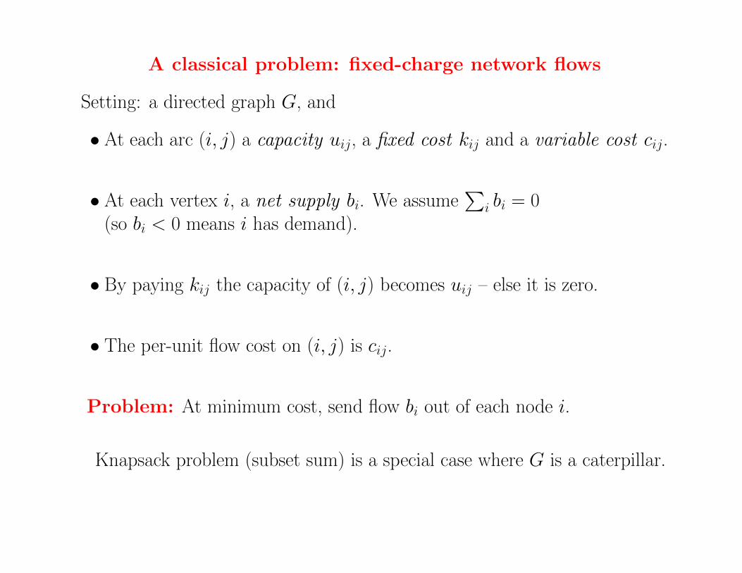
A classical problem: fixed-charge network flows
Setting: a directed graph G, and
• At each arc (i, j) a capacity uij, a fixed cost kij and a variable cost cij.
• At each vertex i, a net supply bi. We assume∑
i bi = 0(so bi < 0 means i has demand).
• By paying kij the capacity of (i, j) becomes uij – else it is zero.
• The per-unit flow cost on (i, j) is cij.
Problem: At minimum cost, send flow bi out of each node i.
Knapsack problem (subset sum) is a special case where G is a caterpillar.

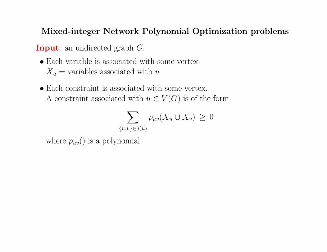
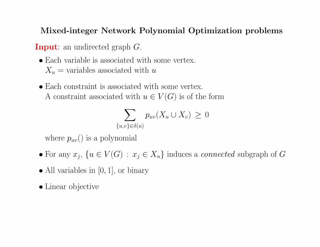
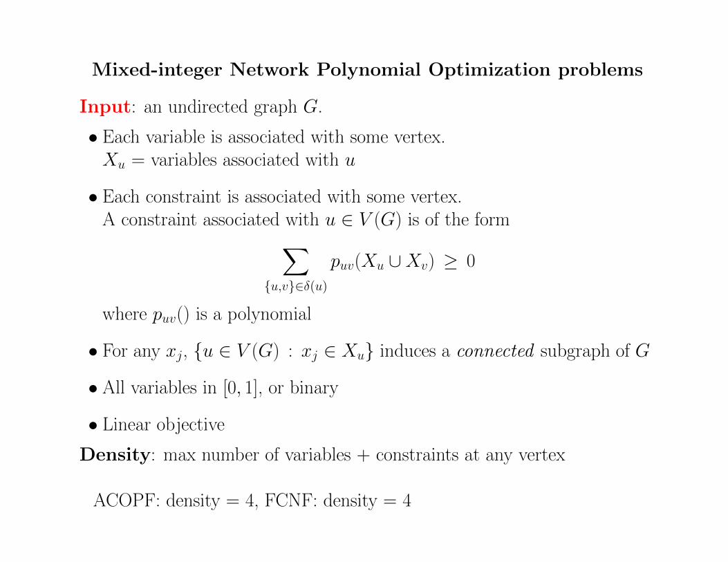
Mixed-integer Network Polynomial Optimization problems
Input: an undirected graph G.
• Each variable is associated with some vertex.Xu = variables associated with u
Mixed-integer Network Polynomial Optimization problems
Input: an undirected graph G.
• Each variable is associated with some vertex.Xu = variables associated with u
• Each constraint is associated with some vertex.A constraint associated with u ∈ V (G) is of the form∑
{u,v}∈δ(u)
puv(Xu ∪Xv) ≥ 0
where puv() is a polynomial
• For any xj, {u ∈ V (G) : xj ∈ Xu} induces a connected subgraph of G
• All variables in [0, 1], or binary
• Linear objective
Density: max number of variables + constraints at any vertex
ACOPF: density = 4, FCNF: density = 4
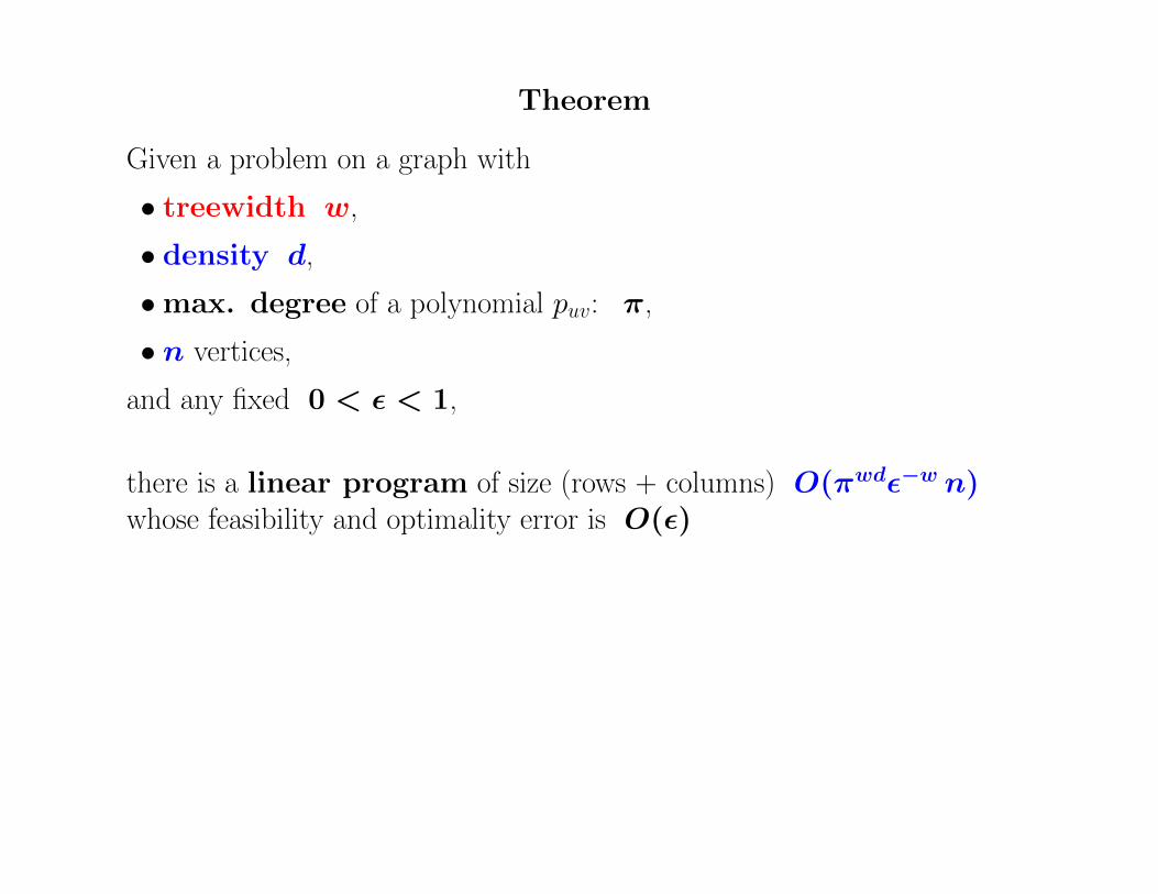
Theorem
Given a problem on a graph with
• treewidth w,
• density d,
•max. degree of a polynomial puv: π,
• n vertices,
and any fixed 0 < ε < 1,
there is a linear program of size (rows + columns) O(πwdε−w n)whose feasibility and optimality error is O(ε)

Theorem
Given a problem on a graph with
• treewidth w,
• density d,
•max. degree of a polynomial puv: π,
• n vertices,
and any fixed 0 < ε < 1,
there is a linear program of size (rows + columns) O(πwdε−w n)whose feasibility and optimality error is O(ε)
• Problem feasible → LP ε-feasibleadditive error = ε times L1 norm of constraintand objective value changes by ε times L1 norm of objective
• And viceversa
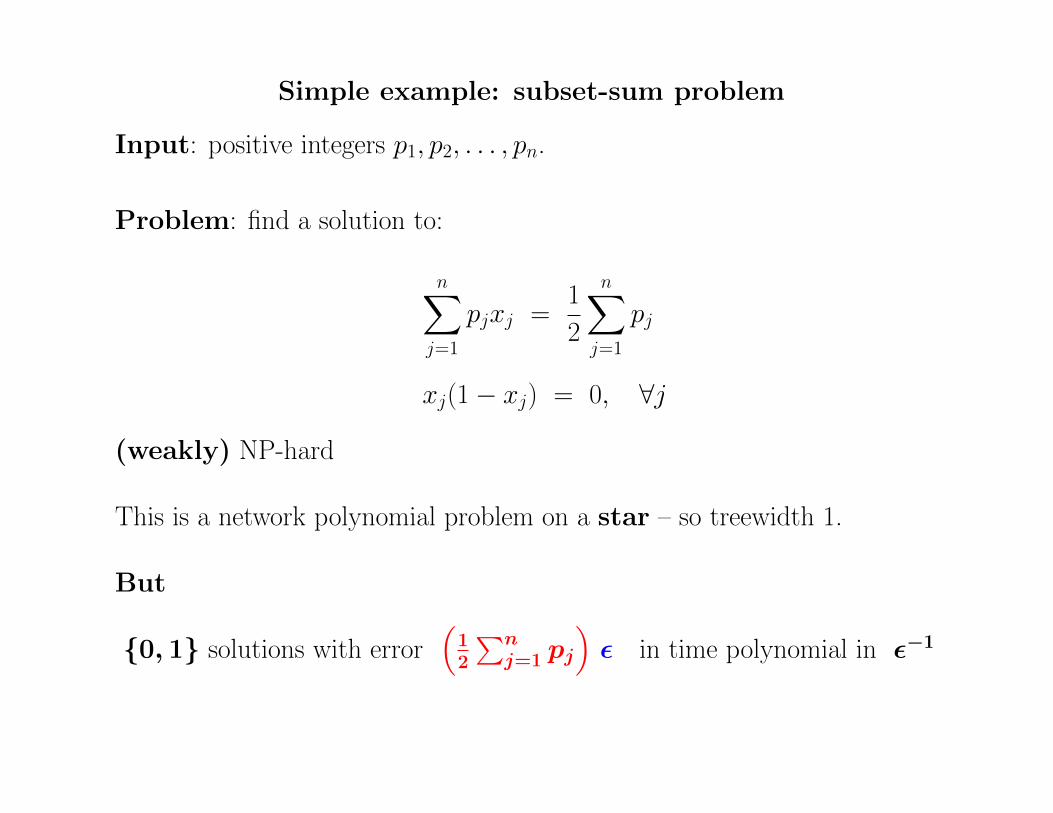
Simple example: subset-sum problem
Input: positive integers p1, p2, . . . , pn.
Problem: find a solution to:
n∑j=1
pjxj =1
2
n∑j=1
pj
xj(1− xj) = 0, ∀j
(weakly) NP-hard
This is a network polynomial problem on a star – so treewidth 1.
But
{0, 1} solutions with error(
12
∑nj=1 pj
)ε in time polynomial in ε−1

More general: (Basic polynomially-constrained mixed-integer LP)
min cTx
s.t. pi(x) ≥ 0 1 ≤ i ≤ m
xj ∈ {0, 1} ∀j ∈ I, 0 ≤ xj ≤ 1, otherwise
Each pi(x) is a polynomial.
Theorem
For any instance where
• the intersection graph has treewidth w,
•max. degree of any pi(x) is π,
• n variables,
and any fixed 0 < ε < 1, there is a linear program of size (rows +columns) O(πwε−w−1 n) whose feasibility and optimality error is O(ε)(abridged).
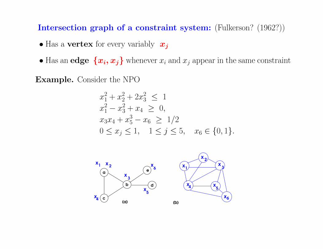
Intersection graph of a constraint system: (Fulkerson? (1962?))
• Has a vertex for every variably xj
• Has an edge {xi, xj} whenever xi and xj appear in the same constraint
Example. Consider the NPO
x21 + x22 + 2x23 ≤ 1
x21 − x23 + x4 ≥ 0,
x3x4 + x35 − x6 ≥ 1/2
0 ≤ xj ≤ 1, 1 ≤ j ≤ 5, x6 ∈ {0, 1}.
x1 x
26
x
x2
x3
x4 x
5
x1
x4
x5
x3
a
b
c
d
e
(a) (b)6x

Main technique: approximation through pure-binaryproblems
Glover, 1975 (abridged)
Let x be a variable, with bounds 0 ≤ x ≤ 1. Let 0 < γ < 1. Then wecan approximate
x ≈∑L
h=1 2−hyh
where each yh is a binary variable. In fact, choosing L = dlog2 γ−1e,
we have
x ≤∑L
h=1 2−hyh ≤ x+ γ.
→ Given a mixed-integer polynomially constrained LPapply this technique to each continuous variable xj
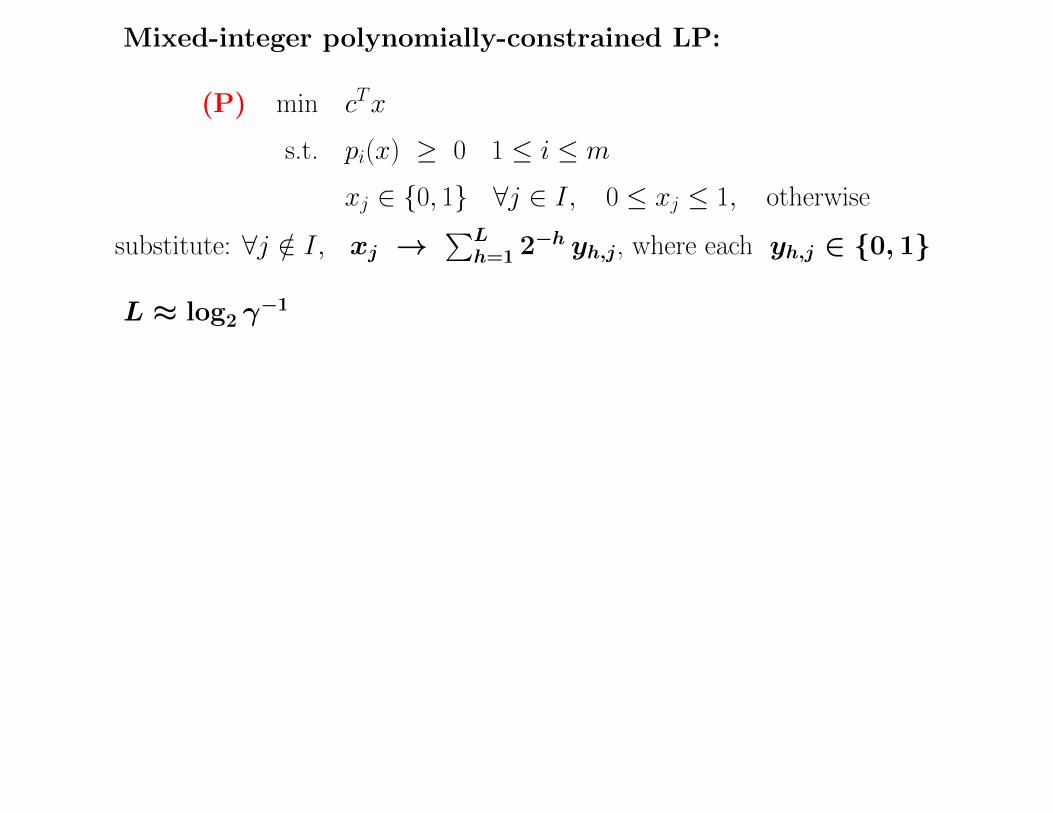
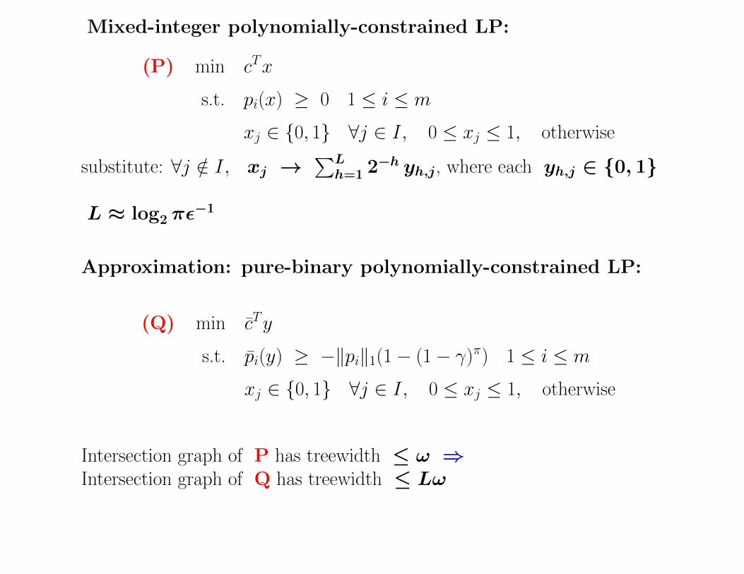
Mixed-integer polynomially-constrained LP:
(P) min cTx
s.t. pi(x) ≥ 0 1 ≤ i ≤ m
xj ∈ {0, 1} ∀j ∈ I, 0 ≤ xj ≤ 1, otherwise
substitute: ∀j /∈ I, xj →∑L
h=1 2−h yh,j, where each yh,j ∈ {0, 1}
L ≈ log2 γ−1
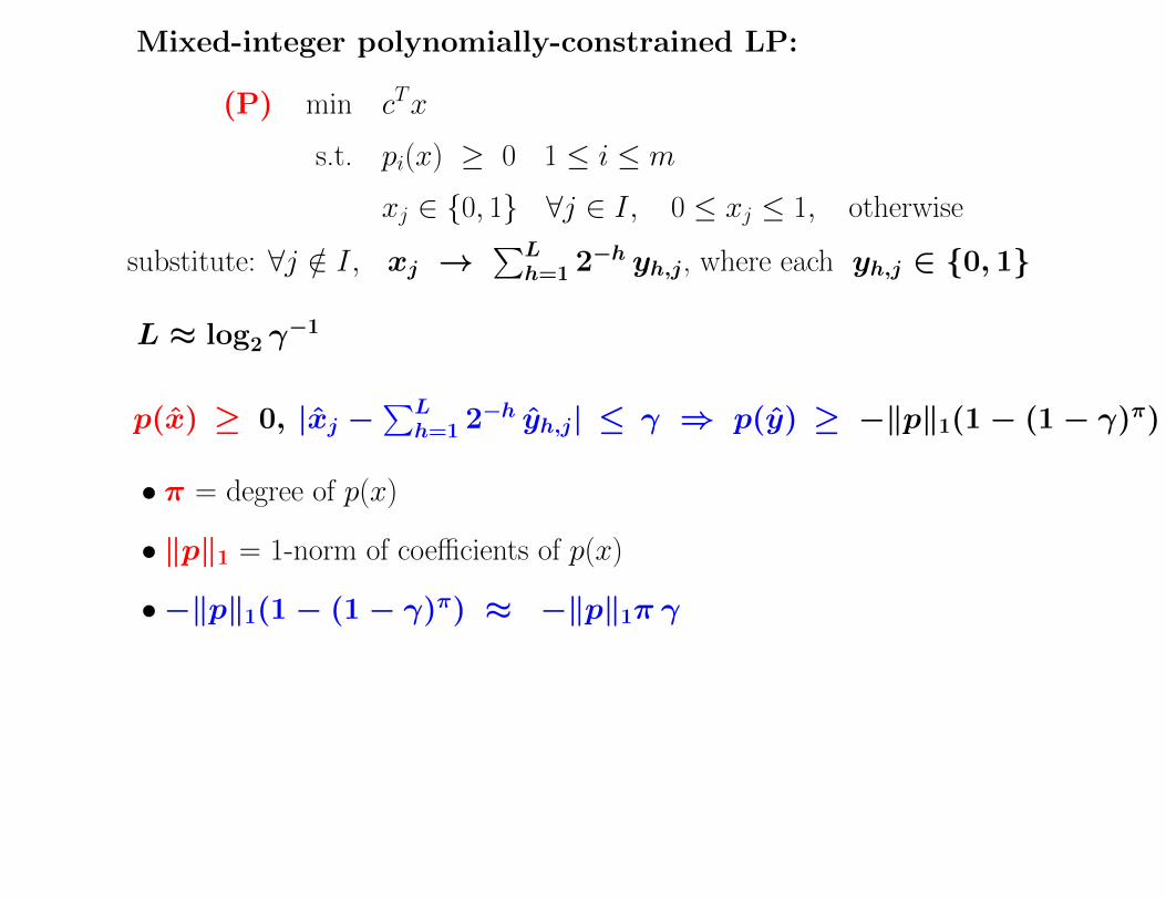
Mixed-integer polynomially-constrained LP:
(P) min cTx
s.t. pi(x) ≥ 0 1 ≤ i ≤ m
xj ∈ {0, 1} ∀j ∈ I, 0 ≤ xj ≤ 1, otherwise
substitute: ∀j /∈ I, xj →∑L
h=1 2−h yh,j, where each yh,j ∈ {0, 1}
L ≈ log2 γ−1
p(x) ≥ 0, |xj −∑L
h=1 2−h yh,j| ≤ γ ⇒ p(y) ≥ −‖p‖1(1− (1− γ)π)
• π = degree of p(x)
• ‖p‖1 = 1-norm of coefficients of p(x)
•−‖p‖1(1− (1− γ)π) ≈ −‖p‖1π γ
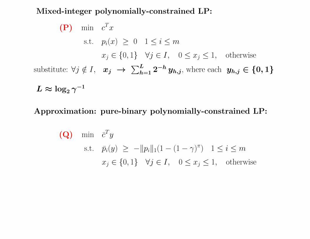
Mixed-integer polynomially-constrained LP:
(P) min cTx
s.t. pi(x) ≥ 0 1 ≤ i ≤ m
xj ∈ {0, 1} ∀j ∈ I, 0 ≤ xj ≤ 1, otherwise
substitute: ∀j /∈ I, xj →∑L
h=1 2−h yh,j, where each yh,j ∈ {0, 1}
L ≈ log2 γ−1
Approximation: pure-binary polynomially-constrained LP:
(Q) min cTy
s.t. pi(y) ≥ −‖pi‖1(1− (1− γ)π) 1 ≤ i ≤ m
xj ∈ {0, 1} ∀j ∈ I, 0 ≤ xj ≤ 1, otherwise
Mixed-integer polynomially-constrained LP:
(P) min cTx
s.t. pi(x) ≥ 0 1 ≤ i ≤ m
xj ∈ {0, 1} ∀j ∈ I, 0 ≤ xj ≤ 1, otherwise
substitute: ∀j /∈ I, xj →∑L
h=1 2−h yh,j, where each yh,j ∈ {0, 1}
L ≈ log2 πε−1
Approximation: pure-binary polynomially-constrained LP:
(Q) min cTy
s.t. pi(y) ≥ −‖pi‖1(1− (1− γ)π) 1 ≤ i ≤ m
xj ∈ {0, 1} ∀j ∈ I, 0 ≤ xj ≤ 1, otherwise
Intersection graph of P has treewidth ≤ ω ⇒Intersection graph of Q has treewidth ≤ Lω

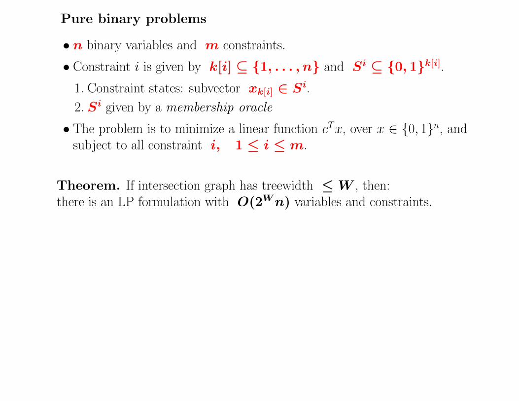
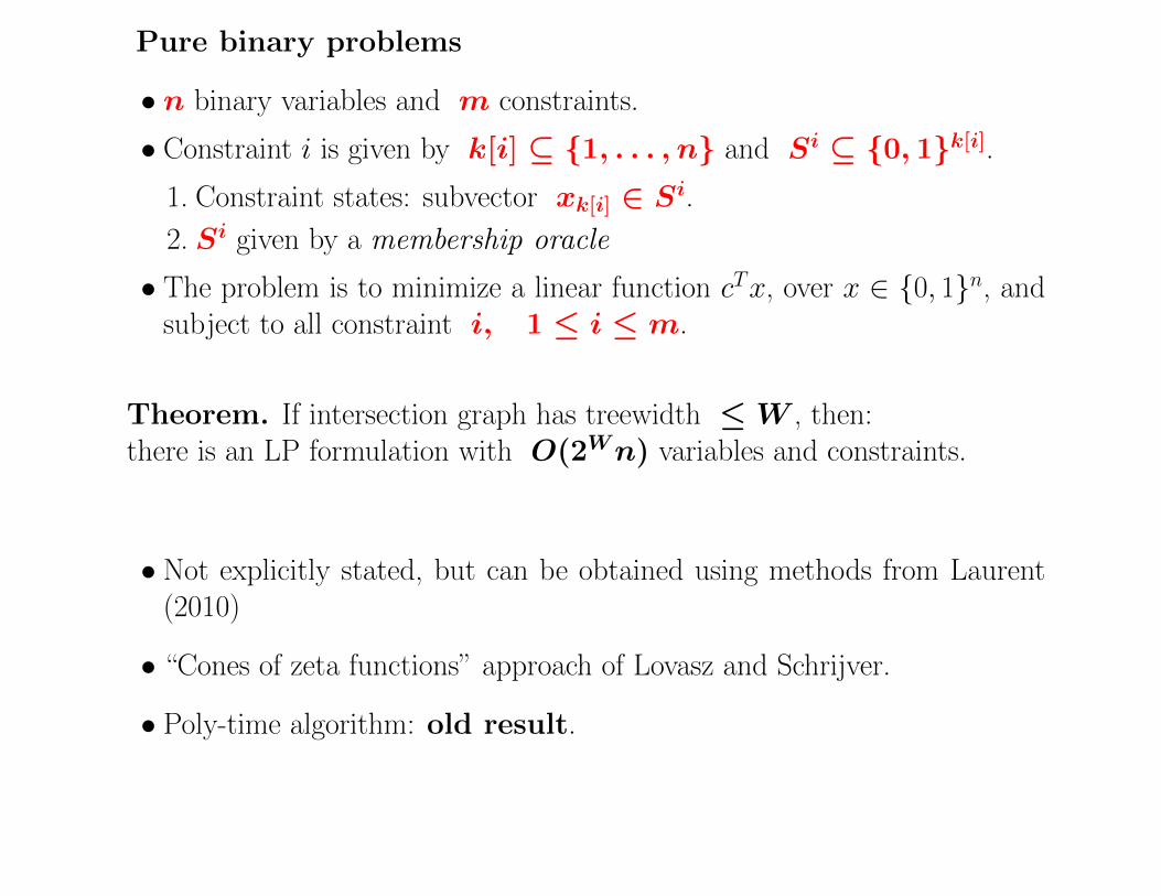
Pure binary problems
• n binary variables and m constraints.
• Constraint i is given by k[i] ⊆ {1, . . . , n} and Si ⊆ {0, 1}k[i].
1. Constraint states: subvector xk[i] ∈ Si.2. Si given by a membership oracle
• The problem is to minimize a linear function cTx, over x ∈ {0, 1}n, andsubject to all constraint i, 1 ≤ i ≤ m.
Theorem. If intersection graph has treewidth ≤W , then:there is an LP formulation with O(2Wn) variables and constraints.
• Not explicitly stated, but can be obtained using methods from Laurent(2010)
• “Cones of zeta functions” approach of Lovasz and Schrijver.
• Poly-time algorithm: old result.

Pure binary problems
min cTx
s.t. xk[i] ∈ Si 1 ≤ i ≤ m,
x ∈ {0, 1}n
Theorem. If intersection graph has treewidth ≤W , then:there is an LP formulation with O(2Wn) variables and constraints.
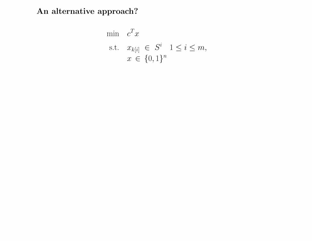
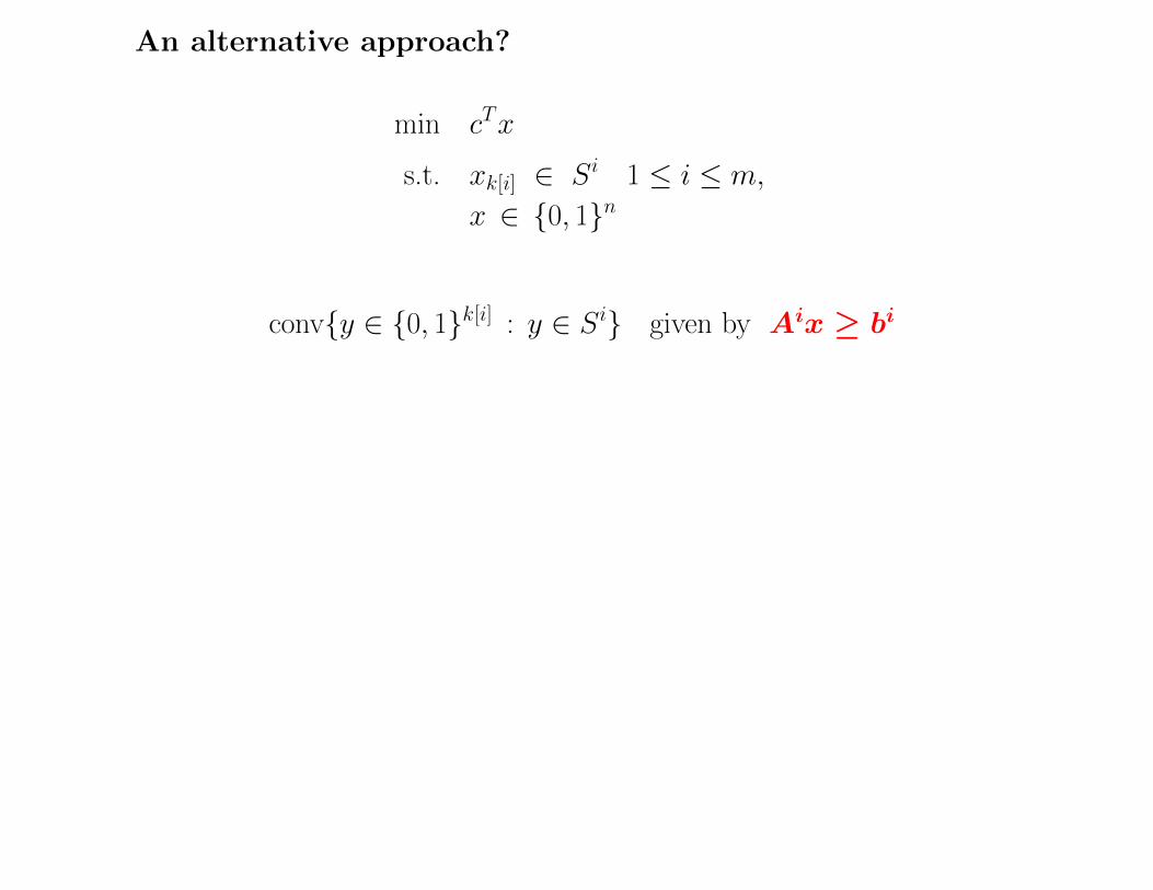
An alternative approach?
min cTx
s.t. xk[i] ∈ Si 1 ≤ i ≤ m,
x ∈ {0, 1}n
An alternative approach?
min cTx
s.t. xk[i] ∈ Si 1 ≤ i ≤ m,
x ∈ {0, 1}n
conv{y ∈ {0, 1}k[i] : y ∈ Si} given by Aix ≥ bi
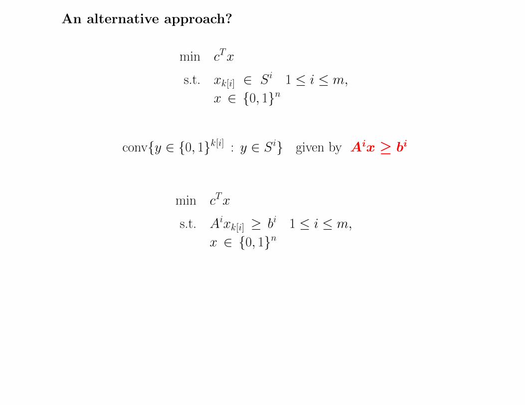
An alternative approach?
min cTx
s.t. xk[i] ∈ Si 1 ≤ i ≤ m,
x ∈ {0, 1}n
conv{y ∈ {0, 1}k[i] : y ∈ Si} given by Aix ≥ bi
min cTx
s.t. Aixk[i] ≥ bi 1 ≤ i ≤ m,
x ∈ {0, 1}n

An alternative approach?
min cTx
s.t. xk[i] ∈ Si 1 ≤ i ≤ m,
x ∈ {0, 1}n
conv{y ∈ {0, 1}k[i] : y ∈ Si} given by Aix ≥ bi
min cTx
s.t. Aixk[i] ≥ bi 1 ≤ i ≤ m,
x ∈ {0, 1}n
But: Barany, Por (2001):
for d large enough, there exist 0,1-polyhedra in Rd with(d
log d
)d/4facets

Corollary: (polynomially-constrained mixed-integer LP)
min cTx
s.t. pi(x) ≥ 0 1 ≤ i ≤ m
xj ∈ {0, 1} ∀j ∈ I, 0 ≤ xj ≤ 1, otherwise
Each pi(x) is a polynomial.
Theorem
For any instance where
• the intersection graph has treewidth w,
•max. degree of any pi(x) is π,
• n variables,
and any fixed 0 < ε < 1, there is a linear program of size (rows +columns) O(πwε−w−1 n) whose feasibility and optimality error is O(ε)(abridged).
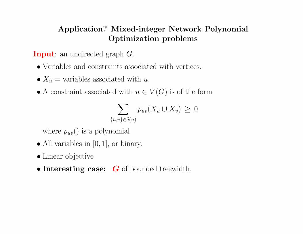
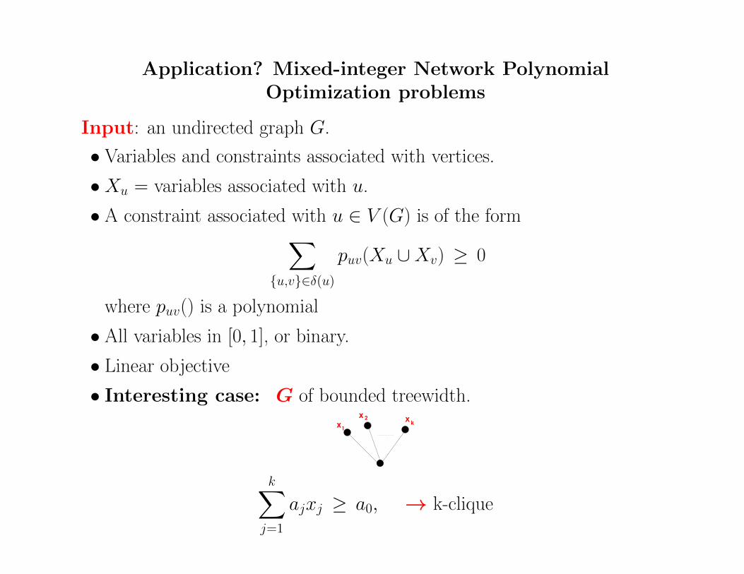
Application? Mixed-integer Network PolynomialOptimization problems
Input: an undirected graph G.
• Variables and constraints associated with vertices.
•Xu = variables associated with u.
• A constraint associated with u ∈ V (G) is of the form∑{u,v}∈δ(u)
puv(Xu ∪Xv) ≥ 0
where puv() is a polynomial
• All variables in [0, 1], or binary.
• Linear objective
• Interesting case: G of bounded treewidth.
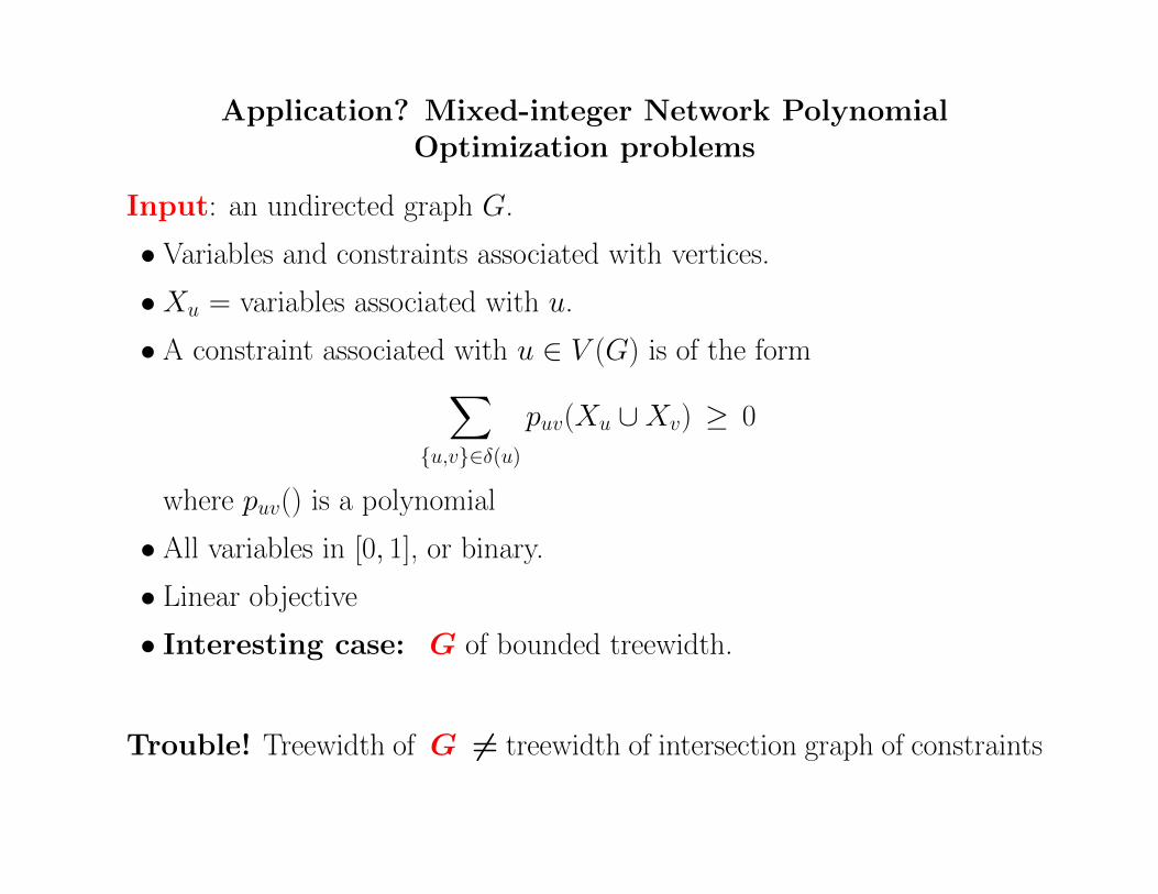
Trouble! Treewidth of G 6= treewidth of intersection graph of constraints
Application? Mixed-integer Network PolynomialOptimization problems
Input: an undirected graph G.
• Variables and constraints associated with vertices.
•Xu = variables associated with u.
• A constraint associated with u ∈ V (G) is of the form∑{u,v}∈δ(u)
puv(Xu ∪Xv) ≥ 0
where puv() is a polynomial
• All variables in [0, 1], or binary.
• Linear objective
• Interesting case: G of bounded treewidth.
x
xx
1
2k
k∑j=1
ajxj ≥ a0, → k-clique

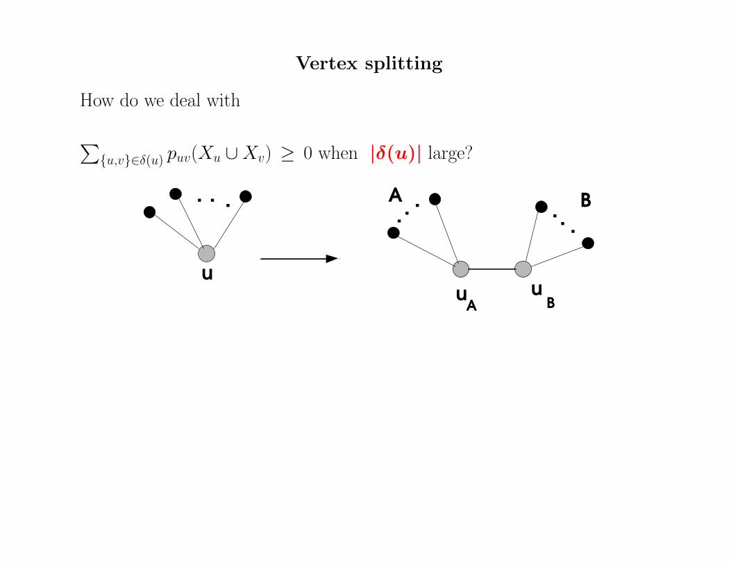
Vertex splitting
How do we deal with
∑{u,v}∈δ(u) puv(Xu ∪Xv) ≥ 0 when |δ(u)| large?
Vertex splitting
How do we deal with
∑{u,v}∈δ(u) puv(Xu ∪Xv) ≥ 0 when |δ(u)| large?
u
. . ....
.. .
A B
uA
uB
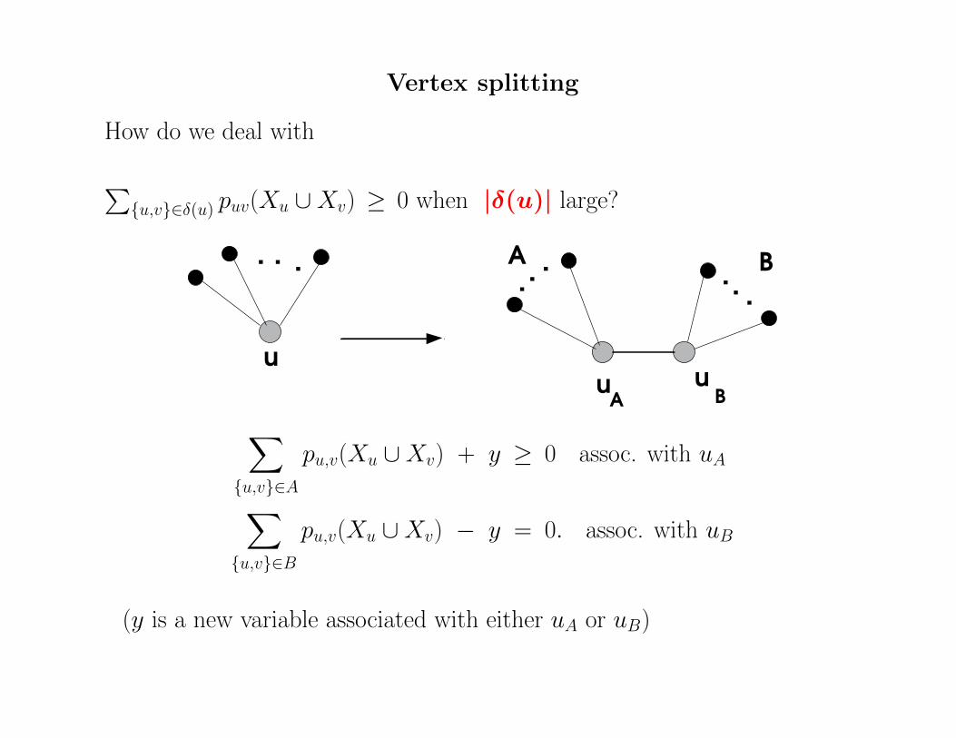
Vertex splitting
How do we deal with
∑{u,v}∈δ(u) puv(Xu ∪Xv) ≥ 0 when |δ(u)| large?
u
. . ....
.. .
A B
uA
uB∑
{u,v}∈A
pu,v(Xu ∪Xv) + y ≥ 0 assoc. with uA
∑{u,v}∈B
pu,v(Xu ∪Xv) − y = 0. assoc. with uB
(y is a new variable associated with either uA or uB)
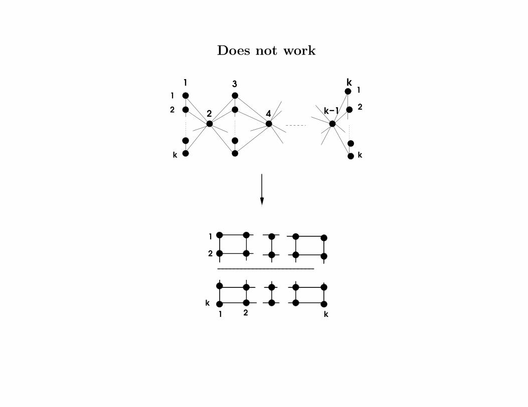
Does not work
k
1
k
2
1
1
2
3
4
k
2
k
1 2
1
2
k
k−1
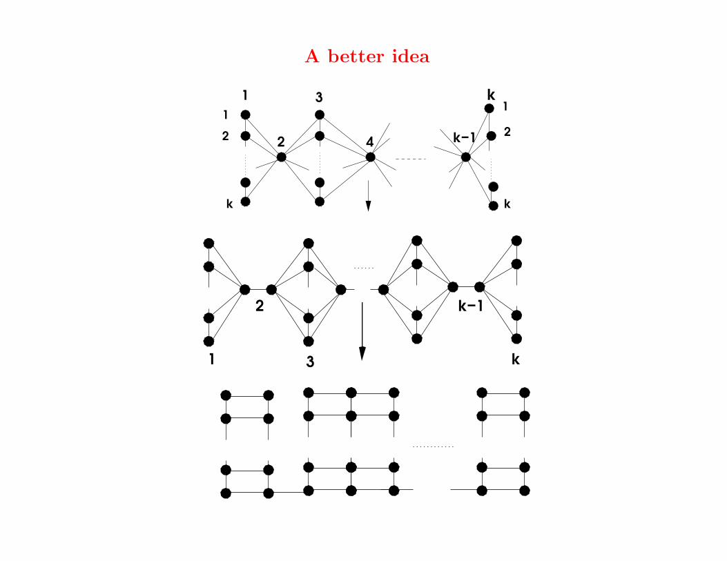
A better idea
k
1
k
2
1
1
2
3
42
k
k−1
1
2
k3
k−1

Theorem
Given a graph of treewidth ≤ ω, there is a sequence of vertex splittingssuch that the resulting graph
• Has treewidth ≤ O(ω)
• Has maximum degree ≤ 3.

Theorem
Given a graph of treewidth ≤ ω, there is a sequence of vertex splittingssuch that the resulting graph
• Has treewidth ≤ O(ω)
• Has maximum degree ≤ 3.
Perhaps known to graph minors people?
Corollary (abridged)
Given a network polynomial optimization problem on a graph G, withtreewidth ≤ ω there is an equivalent problem on a graph H withtreewidth ≤ O(ω) and max degree 3.
Corollary. The intersection graph has treewidth ≤ O(ω).

Tree-width
Let G be an undirected graph with vertices V (G) and edges E(G).
A tree-decomposition of G is a pair (T,Q) where:
• T is a tree. Not a subtree of G, just a tree
• For each vertex t of T , Qt is a subset of V (G). These subsets satisfythe two properties:
(1) For each vertex v of G, the set {t ∈ V (T ) : v ∈ Qt} is a subtreeof T , denoted Tv.
(2) For each edge {u, v} of G, the two subtrees Tu and Tv intersect.
• The width of (T,Q) is maxt∈T |Qt| − 1.
1
2
3
4
5 6
→ two subtrees Tu, Tv may overlap even if {u, v} is not an edge of G
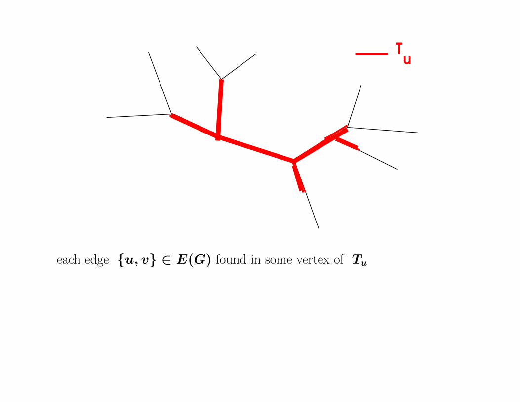
Tu
each edge {u, v} ∈ E(G) found in some vertex of Tu

Tv
Tu
Tu
must intersect only here
for some edge {u,v}
wlog every edge {u, v} ∈ E(G) found in some leaf of Tu
Sat.Nov..7.102812.2015@rockadoodle
Related Documents