Loyalty_Driver_Analysis_V13b

Optimizing Customer Loyalty

An Integrated Market Research Workflow Using Bayesian Networks and BayesiaLab

Stefan Conrady, Managing Partner, Bayesia USA

Dr. Lionel Jouffe, CEO, Bayesia

February 14, 2014

Table of ContentsExecutive Summary

Identifying Priorities for Maximizing Repurchase Intent 4

Challenge: Indistinguishable Drivers of Loyalty 4

Solution: Bayesian Networks as Modeling Framework 4

Implementation 5

Other Benefits 5

Introduction

Background 7

Workflow Overview 8

Latent Factor Induction 8

Multi-Level Analysis 8

Optimization 9

Acknowledgements 10

Notation 10

TutorialSource Data 11

Data Selection 11

Coding 11

Data Import 12

Unsupervised Structural Learning 18

Mapping 24

Missing Values Imputation 25

Variable Clustering 27

Latent Factor Induction via Multiple Clustering 33

Factor States/Values 36

Introducing the Target Node 38


ii www.bayesia.us | www.bayesia.sg

http://www.bayesia.us


http://www.bayesia.sg


Focusing on Factors 40

Supervised Learning 43

Structural Coefficient Analysis 44

Target Mean Analysis 46

Multi-Quadrant Analysis (Total Market ➔ Segment) 50

Full-Size Pickup Segment 55

Multi-Quadrant Analysis (Segment ➔ Model) 60

Relearning the Structure at the Market Level 61

Variations within the Realm of the Possible 69

Optimization 71

Recommendation for GMC Sierra 1500 78

Summary 80

Appendix

Variables 81

List of Factors 82

Contact Information


www.bayesia.us | www.bayesia.sg iii





Executive Summary

Identifying Priorities for Maximizing Repurchase IntentThis tutorial illustrates an innovative market research workflow for deriving marketing and product planning

priorities from auto buyer surveys. In this study, we utilize the Strategic Vision New Vehicle Experience Sur-

vey, which includes, among many other items, customers’ satisfaction ratings with regard to over 100 individ-

ual product attributes.

Challenge: Indistinguishable Drivers of Loyalty

With traditional statistical methods, it has been difficult to

rank the importance of individual product attribute ratings

with regard to an overall measure, such as repurchase loy-

alty.

The key challenge is that customers’ ratings of individual

product attributes are highly correlated. When plotted, we

see 100 lines that are nearly indistinguishable in terms of

their slope. Given this collinearity of all variables, traditional

statistical methods fail to distinguish the importance of in-

dividual ratings. We could only naively conclude that an

improvement in any rating would generally be associated with higher loyalty. No clear priorities could be

established on such a basis.

Solution: Bayesian Networks as Modeling Framework

To overcome this problem we employ an alternative framework: we use Bayesian networks as the mathe-

matical formalism, plus the machine-learning and optimization algorithms of the BayesiaLab software pack-

age. This approach embraces collinearity as a feature in the model, instead of suppressing it as a nuisance.


4 www.bayesia.us | www.bayesia.sg





Implementation

First, using BayesiaLab, we machine-learn a Bayesian network that models customers’ brand loyalty as a func-

tion of their ratings of their current vehicle. This identifies key factors as loyalty drivers in the overall market,

at the segment level, and finally at the model level. With these factors identified, we perform optimization, for

each vehicle within its competitive context. As a result, we obtain a list of specific priorities for each vehicle,

along with the simulated gain in loyalty.

Other Benefits

No Black Box

Many modeling techniques offered in the field of marketing science are opaque to the end user of the re-

search. The nature of many models make them inherently black-box, and thus require a leap of faith by the

decision maker.


www.bayesia.us | www.bayesia.sg 5





Not so in our research framework with Bayesian networks. Regardless of one’s quantitative skills, any subject

matter expert can—by simply using common sense—interpret the Bayesian network models generated with

our workflow. Any stakeholder can immediately scrutinize such a model, thus enabling him to verify its struc-

ture, or, by using his domain knowledge, to invalidate it. Their inherent falsifiability makes Bayesian networks

ideal scientific tools.

Real-Time Recommendations

In most organizations, waiting for research results and their interpretation is a matter of months. The time

span between a consumer sentiment expressed in a survey, and a company’s response, can sometimes even

exceed the lifecycle length of a product.

Our workflow creates a single, direct, and transparent link from data to recommendation. This directness pro-

vides unprecedented analysis speed. We reduce the lag between receipt of data and delivery of recommenda-

tion from months to days. As a result, near real-time policy recommendations are feasible for the first time.







Introduction

Background

Market Maturity and Homogeneity

The auto industry is an example of a very mature market. It is fair to say that all automakers offer high-

quality products these days in North America. The proverbial “lemons” are few and far between. Fierce com-

petition has led to product offerings that are remarkably similar for their respective vehicle category, both in

their specifications and their functional performance. With similar cost and budget constraints, and an over-

lapping supplier base for all manufacturers, the auto business is mostly about eking out minute advantages,

as opposed creating fundamental breakthroughs.

No doubt, the brand plays a major role in buying decisions. Hence, marketing, branding and promotion efforts

of automakers typically absorb a similar amount of resources as the actual R&D expenses for vehicle devel-

opment. For the purpose of this paper, however, we will not venture into the challenging domain of return on

marketing investment. This is a topic for another methodology tutorial in the future.

Given this overall quality and performance homogeneity, consumer perceptions—as we will see in this

study—are also remarkably homogenous across similar kinds of vehicles. For market researchers, it is thus

very difficult to “tease out” material differences in customers’ perception of product attributes of competitive

vehicles. It is even more challenging to establish which of these similarly-perceived vehicle characteristics do

really matter when it comes to buying an automobile.

Loyalty

“It is cheaper to keep a customer than to find a new one” is an often-quoted marketing adage. Loyalty is a

very relevant quantity, much more tangible than mere satisfaction. Given the maturity of the auto market and

rather lengthy ownership cycles, repurchase loyalty is of special significance. Thus, we go beyond satisfaction

in this study, and rather link product ratings to stated repurchase intent.

We will focus exclusively on how customers’ product ratings can affect loyalty, i.e. find “what really matters”

when it come to brand loyalty. We will present a methodology that can identify the relevance of minute dif-

ferences in consumer perception, in order to help identify priorities among a plethora of opportunities to im-

prove product ratings.







Workflow Overview

Latent Factor Induction

In this paper, we employ BayesiaLab’s machine learning algorithms to generate Bayesian networks that will

allow us to identify major concepts, i.e. latent factors, from the observed satisfaction ratings, i.e. manifest

variables. Inducing factors creates a level of abstraction that will allow us to see a “bigger picture,” that is

more stable than if it is only based on manifest variables. Once factors are identified, we will examine how

they “drive” brand loyalty. Ultimately, we want to establish the effect of these factors with regard to the out-

come variable, i.e. loyalty.

Multi-Level Analysis

We will examine the loyalty drivers at multiple levels of the market. We will identify the general areas of

opportunity for loyalty improvement at the segment1 level and at the vehicle model2 level.



1 “Segment” refers to a vehicle category, such as Subcompacts or Large Sedans. There are numerous segmentation schemes

used in the auto industry, which all relyon custom terminology. However, all automakers agree on the definition of the

Full-Size Pickup segment, on which we focus in this study.

2 “Vehicle model” refers to a vehicle make (brand) and model/line, e.g. Ford Explorer, Nissan Altima. In this case study, we

will not drill down to the vehicle trim level, e.g. Ford Explorer Limited and Nissan Altima 2.5 S.





More specifically, we will proceed from the overall market to the Full-Size Pickup segment, and then to the

vehicle models within it. We chose this particular segment primarily for expository simplicity. It is a very well

defined segment in terms of vehicle characteristics while only consisting of a few major contenders. Plus, it is

one of the most important segments in the U.S. auto industry, both in terms of volume and profitability.

Optimization

Once loyalty drivers are modeled, we will identify priorities for improvements by vehicle model. For each

model, in its specific competitive context, our approach will generate recommendations with the objective of

improving brand loyalty.

As we examine the impact of satisfaction ratings on loyalty, we need to remember though that satisfaction

ratings are inherently subjective. The recommendations we will present do not necessarily specify the means

by which ratings should be improved.

TotalMarket

Small Car

Full-Size Pickup

Luxury Car

Mid-Size Crossover Utility

Mid-Size Traditional Utility Near-Luxury

Toyota Tundra

Nissan Titan

Ford F-150

GMC Sierra 1500

Dodge Ram

Chevrolet Silverado

Minivan Large Car …

…

…







AcknowledgementsWe would like to express our gratitude to Alexander Edwards, President of Strategic Vision, Inc.3, for gener-

ously providing data from their 2009 New Vehicle Experience Survey for our case study.

NotationTo clearly distinguish between natural language, software-specific functions and example-specific variable

names, the following notation is used:

• Bayesian network and BayesiaLab-specific functions, keywords, commands, etc., are capitalized and shown

in bold type.

• Names of attributes, variables, nodes and names of node states are italicized.



3 Strategic Vision is a research-based consultancy with more than 35 years of experience in understanding the consum-

ers’ and constituents’ decision-making systems for a variety of Fortune 100 clients, 10 Downing Street, Coca-Cola, Ameri-

can Airlines, Proctor & Gamble, the White House and including most automotive manufacturers and many advertising

agencies. The company specializes in identifying consumers’ complete, motivational hierarchies, including the product

attributes, personal benefits, value/emotions and images that drive perceptions and behaviors. Strategic Vision has at its

core a large-scale syndicated automotive experience and “Pulse of the Customer” (POC) study that collects more than

350,000 responses annually, using over 1,500 comprehensive data points Since its foundation in 1972 and incorporation

in 1989, Strategic Vision—led by company founders Darrel Edwards, Ph.D., J. Susan Johnson, Sharon Shedroff, with Alexan-

der Edwards—has used in-depth Discovery Interviews and Value Centered Survey instruments that provide comprehen-

sive, integrated and actionable outcomes, linking behavior to attributes to consequences to values and emotions to im-

ages (www.strategicvision.com).





http://www.strategicvision.com

http://www.strategicvision.com

Tutorial

Source Data

Our case study uses real-world data from the auto industry, which has conducted customer satisfaction re-

search for decades. More specifically, we utilize the 2009 New Vehicle Experience Survey (NVES), a syndicated

study conducted by Strategic Vision, Inc., which surveys new vehicle buyers in the U.S. This study is widely

used in the auto industry, and it is one of principal resources for market researchers and product planners.

NVES contains over 1,000 variables and close to 200,000 respondent records. Among many demographic and

psychographic variables, NVES contains 98 individual satisfaction measures, ranging from Acceleration to

Wiper System Controls.

Data Selection

From the original NVES dataset consisting of 1,089 columns and 71,200 rows, we select 103 columns that are

relevant for the purposes of this tutorial.4

The first group of columns refers to the vehicle type, e.g. make, model and vehicle segment. The second group

includes 98 columns that all concern the vehicle buyer’s satisfaction with specific aspects of the purchased

vehicle, ranging from Ability to Control Sound to Wiper System Controls.

For notational convenience, we rename a number of frequently used variables as follows:

• New Model Segment ➔ Segment

• New Model Purchased - Brand ➔ Make

• New Model Purchased (Alpha Order) ➔ Make/Model

• Rate Buy Another From Same Manufac. ➔ Loyalty

Coding

NVES measures all satisfaction-related variables on an ordinal scale, from 1 (A failure) to 5 (Delightful), as

shown in the excerpt from the printed questionnaire.



4 See the appendix for a complete list of the selected variables.





For analysis purposes, most market researchers have typically been using the NVES satisfaction ratings line-

arly transformed into a 1.5‑9.5 scale. We will follow this convention in our tutorial.

Loyalty is asked in the NVES with the following question, which also features an ordinal scale for the re-

sponse, ranging from Definitely will not to Definitely will.

Given that our objective is loyalty optimization, we need to associate a numerical value with each of the or-

dinal states of this response variable. The following linear assignment of probabilities is somewhat arbitrary,

but for the purpose of this study we will accept it as a reasonable approximation.

Response ProbabilityDefinitely)Will)Not 0.00Probably)Will)Not 0.25Do)Not)Know 0.50Probably)Will 0.75Definitely)Will 1.00

Data Import

To start the analysis with BayesiaLab, we first import the survey data set, which was provided as a CSV file.5

With Data | Open Data Source | Text File, we start the Data Import Wizard, which immediately provides a pre-

view of the data file.



5 CSV stands for “comma-separated values”, a common format for text-based data files.





The table displayed in the Data Import wizard shows the individual variables as columns and the responses

as rows. There are a number of options available, e.g. for sampling. However, this is not necessary in our ex-

ample given the relatively small size of the database.

Clicking the Next button, prompts a data type analysis, which provides BayesiaLab’s best guess regarding the

data type of each variable.







Furthermore, the Information box provides a brief summary regarding the number of records, the number of

missing values 6, filtered states, etc.

In this example, we will need to override the default data type for the Combined Base Rate variable. This vari-

able serves as the survey weight of each observation. We change the data type by highlighting the column

and clicking the Weight check box, which changes the color of the Combined Base Rate column to green.



6 There are no missing values in our database and filtered states are not applicable in this survey.





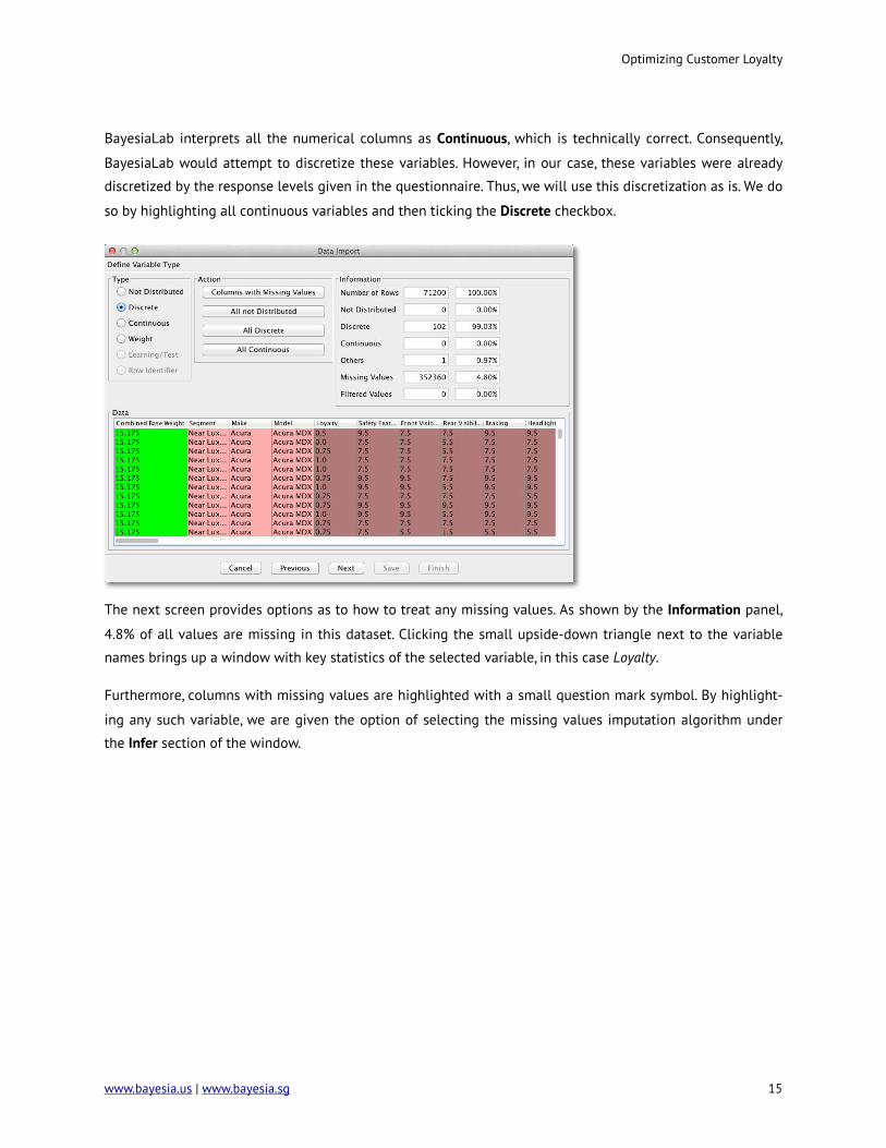
BayesiaLab interprets all the numerical columns as Continuous, which is technically correct. Consequently,

BayesiaLab would attempt to discretize these variables. However, in our case, these variables were already

discretized by the response levels given in the questionnaire. Thus, we will use this discretization as is. We do

so by highlighting all continuous variables and then ticking the Discrete checkbox.

The next screen provides options as to how to treat any missing values. As shown by the Information panel,

4.8% of all values are missing in this dataset. Clicking the small upside-down triangle next to the variable

names brings up a window with key statistics of the selected variable, in this case Loyalty.

Furthermore, columns with missing values are highlighted with a small question mark symbol. By highlight-

ing any such variable, we are given the option of selecting the missing values imputation algorithm under

the Infer section of the window.







Given that we are using weights in this dataset, we now have an option to Normalize Weights. If we left this

option unchecked, each record in the dataset would be counted as many times as the weight indicates. For

instance, the first row would be counted 15.175 times. Applied to all rows, this would yield the correct pro-

portion of observations relative to each other. However, BayesiaLab would subsequently end up “over-

learning” from 3,233,840.85 weighted observations.7 To avoid generating a false sense of precision, we select

Normalize Weights, so each response, on average, represents one transaction.



7 Each response in this survey, on average, represents roughly 45 vehicle purchases.





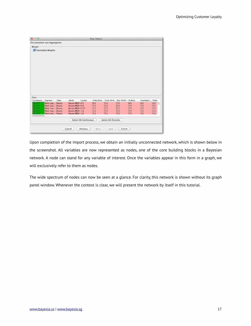
Upon completion of the import process, we obtain an initially unconnected network, which is shown below in

the screenshot. All variables are now represented as nodes, one of the core building blocks in a Bayesian

network. A node can stand for any variable of interest. Once the variables appear in this form in a graph, we

will exclusively refer to them as nodes.

The wide spectrum of nodes can now be seen at a glance. For clarity, this network is shown without its graph

panel window. Whenever the context is clear, we will present the network by itself in this tutorial.







Unsupervised Structural Learning

A central element in our study is to look for overarching concepts among the 98 satisfaction measures in our

data set. Once identified, these concepts will subsequently serve as factors as we further develop our model.







Machine learning a Bayesian network is a remarkably practical way to identify easily-interpretable variable

clusters for factor induction. Among BayesiaLab’s Unsupervised Learning algorithms, the Maximum Weight

Spanning Tree is a very efficient approach for quickly obtaining a Bayesian network that can provide the ba-

sis for variable clustering. The speed of this particular method is due to a key constraint, namely that in the

to-be-learned network, each node is restricted to having only one parent node. This massively reduces the

number of candidate networks that the learning algorithm must examine.

Prior to initiating the clustering process, we need to exclude any nodes that we do not want to be included in

the clustering, such as the node that we will later use as target node and those that we will use as breakout

variables, e.g. Segment. We exclude them by right-clicking on any of the selected nodes and then clicking

Properties | Exclusion from the contextual menu. Alternatively, holding “x” while double-clicking the nodes

performs the same exclusion function. Once excluded, the nodes will appear as .

Now we can start the learning process from the main menu: Learning | Unsupervised Structural Learning |

Maximum Spanning Tree.







The Maximum Weight Spanning Tree is the only learning algorithm in BayesiaLab that offers an alternative

to the Minimum Description Length (MDL) as the learning score. However, without further explanation, we

will stick to the default and confirm MDL.

This default view of the resulting network is hardly intuitive. Hence, throughout this exercise, we will make

frequent use of one of several available layout algorithms.







All layout algorithms are accessible from the main menu via View | Layout. Most often, we will use View |

Automatic Layout, or alternatively use the shortcut “P”.







Upon applying a layout algorithm, we obtain an untangled version of the original network. Note that the

structure of the network remains unchanged. We can further adjust the positions of the nodes as needed to

create a legible and interpretable layout.







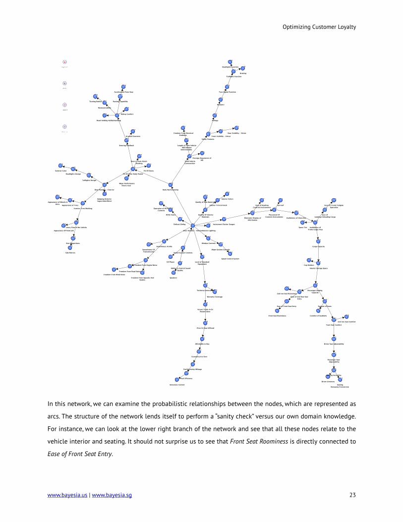
In this network, we can examine the probabilistic relationships between the nodes, which are represented as

arcs. The structure of the network lends itself to perform a “sanity check” versus our own domain knowledge.

For instance, we can look at the lower right branch of the network and see that all these nodes relate to the

vehicle interior and seating. It should not surprise us to see that Front Seat Roominess is directly connected to

Ease of Front Seat Entry.







Mapping

Beyond this kind of qualitative assessment, BayesiaLab’s Mapping function is very helpful for interpreting the

importance of the nodes and the strength of the relationships between them.

We can initiate Mapping from within the Validation Mode by selecting Analysis | Visual | Mapping.

The Mapping window features drop-down menus for Node Analysis and Arc Analysis. We select Node Force

for Node Analysis; for Arc Analysis with choose Mutual Information.







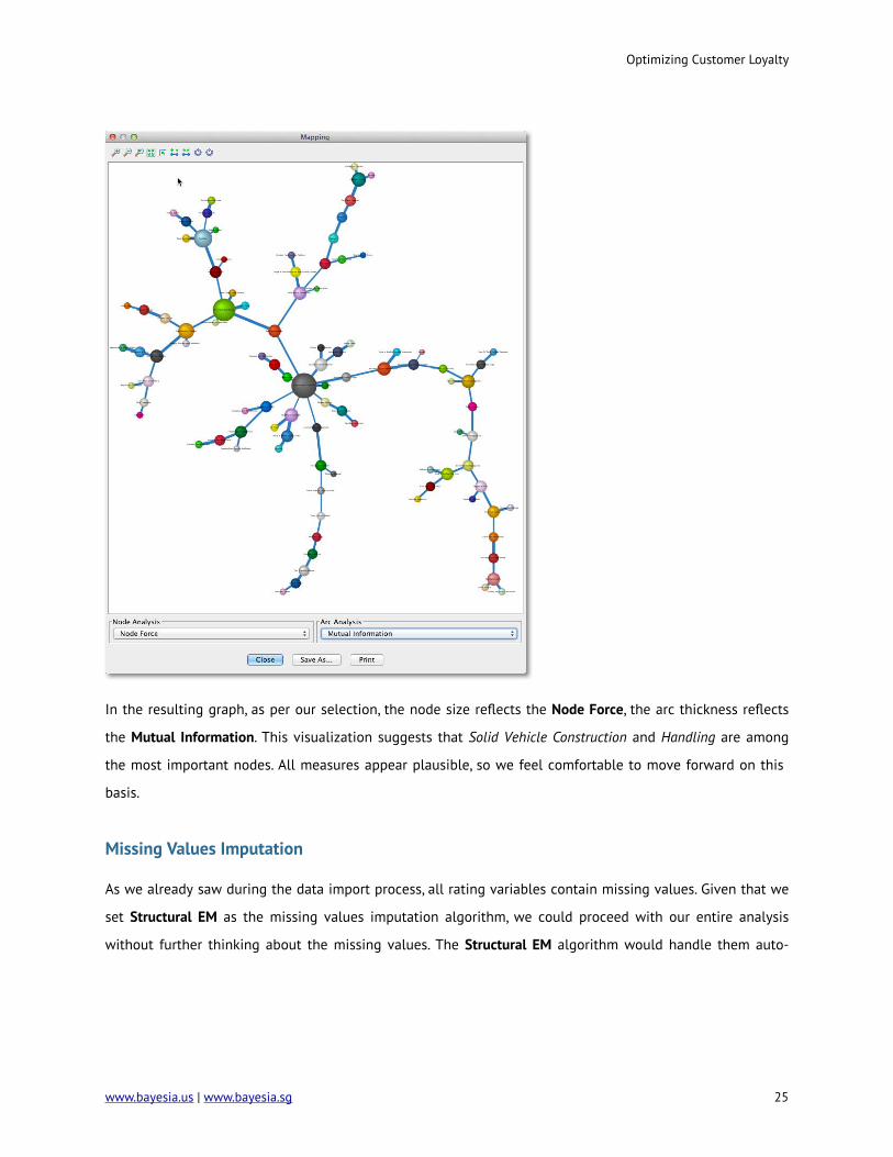
In the resulting graph, as per our selection, the node size reflects the Node Force, the arc thickness reflects

the Mutual Information. This visualization suggests that Solid Vehicle Construction and Handling are among

the most important nodes. All measures appear plausible, so we feel comfortable to move forward on this

basis.

Missing Values Imputation

As we already saw during the data import process, all rating variables contain missing values. Given that we

set Structural EM as the missing values imputation algorithm, we could proceed with our entire analysis

without further thinking about the missing values. The Structural EM algorithm would handle them auto-







matically as we go along.8 However, there is a significant computational burden associated with this ongoing

computation.

In order to accelerate all subsequent tasks, we will fix the most recent imputation that was generated during

the learning of the Maximum Weight Spanning Tree.

To perform this imputation, we first select all nodes, then right-click on any one of the nodes with missing

values, and finally select Imputation from the Contextual Menu.

We are given are a choice of modes, of which we select Standard and Choose the States According to the

Law.

Upon completion of the process, all question marks disappear from the network, indicating that there are no

more missing values.



8 For more details, please see our white paper on missing values processing with Bayesian networks:

http://bayesia.us/missing-values-processing-with-bayesian-networks.html







Variable Clustering

The network, as we see it here, is intended only as an interim step. For product planning or decision-making

purposes, it would indeed be difficult to work directly with 98 manifest nodes. We would not be able to see

the proverbial forest for all the trees. Rather, this network will serve as the basis for Variable Clustering, i.e.

grouping nodes into meaningful concepts.

We start this clustering process, from within the Validation Mode, by selecting Learning | Clustering | Variable

Clustering (or by using the keyboard shortcut “S”).

We now see the same graph as before; however, the nodes are now colored as per their proposed cluster

membership. In our case, BayesiaLab suggests 26 clusters, as indicated in the menu bar.







We can move the slider to change the number of clusters (or by clicking the arrow buttons). This allows us to

align the number of clusters with our domain knowledge. As we change the number, the node colors are

automatically updated.

Additionally, we can view a dendrogram (click to activate) while we adjust the number of clusters. Two

dendrograms are shown below; one with 27 clusters (left) and one with 10 clusters (right).













Alternatively, we can show the currently selected clustering in a similar way as in the previously-introduced

Mapping function. Click in the menu bar to show this view:

For an easier interpretation of these “bubbles”, we can attach labels to them. Since each bubble represents a

cluster of nodes, we select Display Best Node Name from the Contextual Menu.

This shows the name of the node that most strongly contributes to each cluster, given the currently selected

number of clusters.







Two screenshots are shown as examples, based on 24 and 10 clusters respectively.

With Dendrogram and Mapping, we can visually experiment until the appropriate cluster number is estab-

lished. The final selection of the number of clusters remains the task of the analyst. There is no hard-and-fast

rule for choosing the number of clusters as this example illustrates. For instance, is it appropriate to cluster

nodes related to noise with nodes related to smoothness? Two alternative Dendrograms are shown below.

Only a domain expert can make a judgment in this regard.







The number of clusters automatically proposed by BayesiaLab is based on two heuristics: the first is based on

the strength of the relationships, the second on the maximum number of variables per cluster. Whereas we

generally do not advise changing the former, the latter can be modified via Options | Settings | Learning |

Variable Clustering.

After further review of all diagrams, we conclude that 24 clusters are most appropriate for this domain and

confirm this choice by clicking the Validate Clustering button.

Furthermore, we confirm that we want to keep the colors from the just-completed interactive clustering.







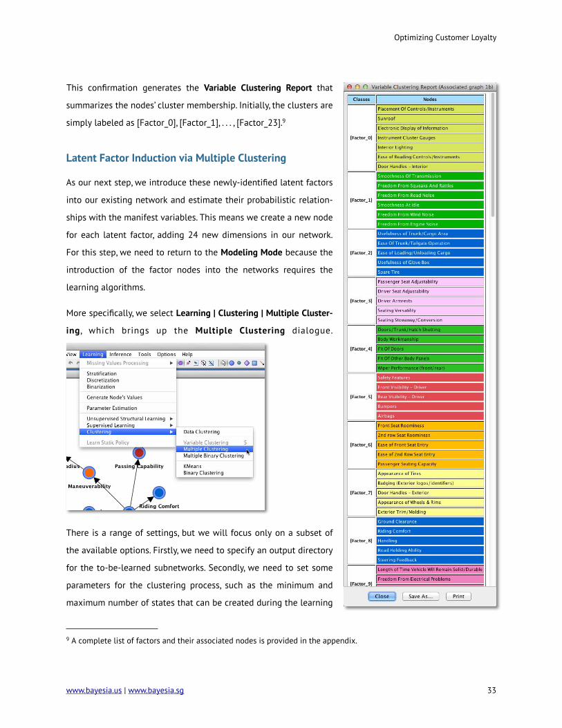
This confirmation generates the Variable Clustering Report that

summarizes the nodes’ cluster membership. Initially, the clusters are

simply labeled as [Factor_0], [Factor_1], . . . , [Factor_23].9

Latent Factor Induction via Multiple Clustering

As our next step, we introduce these newly-identified latent factors

into our existing network and estimate their probabilistic relation-

ships with the manifest variables. This means we create a new node

for each latent factor, adding 24 new dimensions in our network.

For this step, we need to return to the Modeling Mode because the

introduction of the factor nodes into the networks requires the

learning algorithms.

More specifically, we select Learning | Clustering | Multiple Cluster-

ing , which brings up the Multiple Clustering dialogue.

There is a range of settings, but we will focus only on a subset of

the available options. Firstly, we need to specify an output directory

for the to-be-learned subnetworks. Secondly, we need to set some

parameters for the clustering process, such as the minimum and

maximum number of states that can be created during the learning



9 A complete list of factors and their associated nodes is provided in the appendix.





process. For our example, we select Automatic Selection of the Number of Classes, which will allow the learn-

ing algorithm to find the optimum number of factor states up to a maximum of five states. This means that

each new factor will need to represent the corresponding manifest variables with up to five states.

Upon completion of the Multiple Clustering process, we obtain a new network file that contains one small

network for each cluster, with one factor being at the center of each cluster.







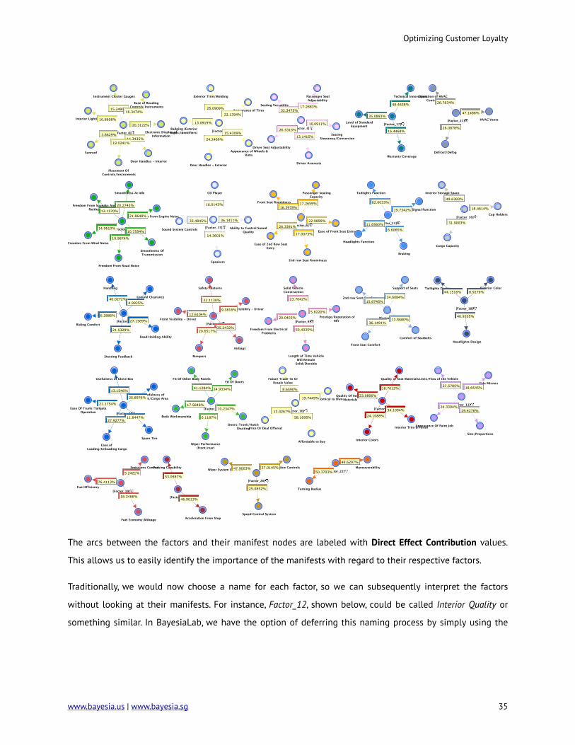
The arcs between the factors and their manifest nodes are labeled with Direct Effect Contribution values.

This allows us to easily identify the importance of the manifests with regard to their respective factors.

Traditionally, we would now choose a name for each factor, so we can subsequently interpret the factors

without looking at their manifests. For instance, Factor_12, shown below, could be called Interior Quality or

something similar. In BayesiaLab, we have the option of deferring this naming process by simply using the







“strongest” node, as per the Direct Effect Contribution value, within each factor cluster as that factor’s Node

Comment.

Clicking Display Node Comments in the menu bar will reveal Interior_Trim & Finish_(4) as a label on the fac-

tor. The suffix “(4)” indicates that 4 manifest variables are linked to this factor.

Factor States/Values

Beyond adding the factors to the network, the Multiple Clustering process has also generated states for all

factors and computed their values. Inducing a factor means finding an appropriate summary of the underlying

joint probability distribution defined by the manifest nodes. In the previous example of Factor_12, this would

mean that the states of Factor_12 can summarize the following four nodes: Interior Trim & Finish, Quality of

Interior Materials, Interior Colors, and Quality of Seat Materials.







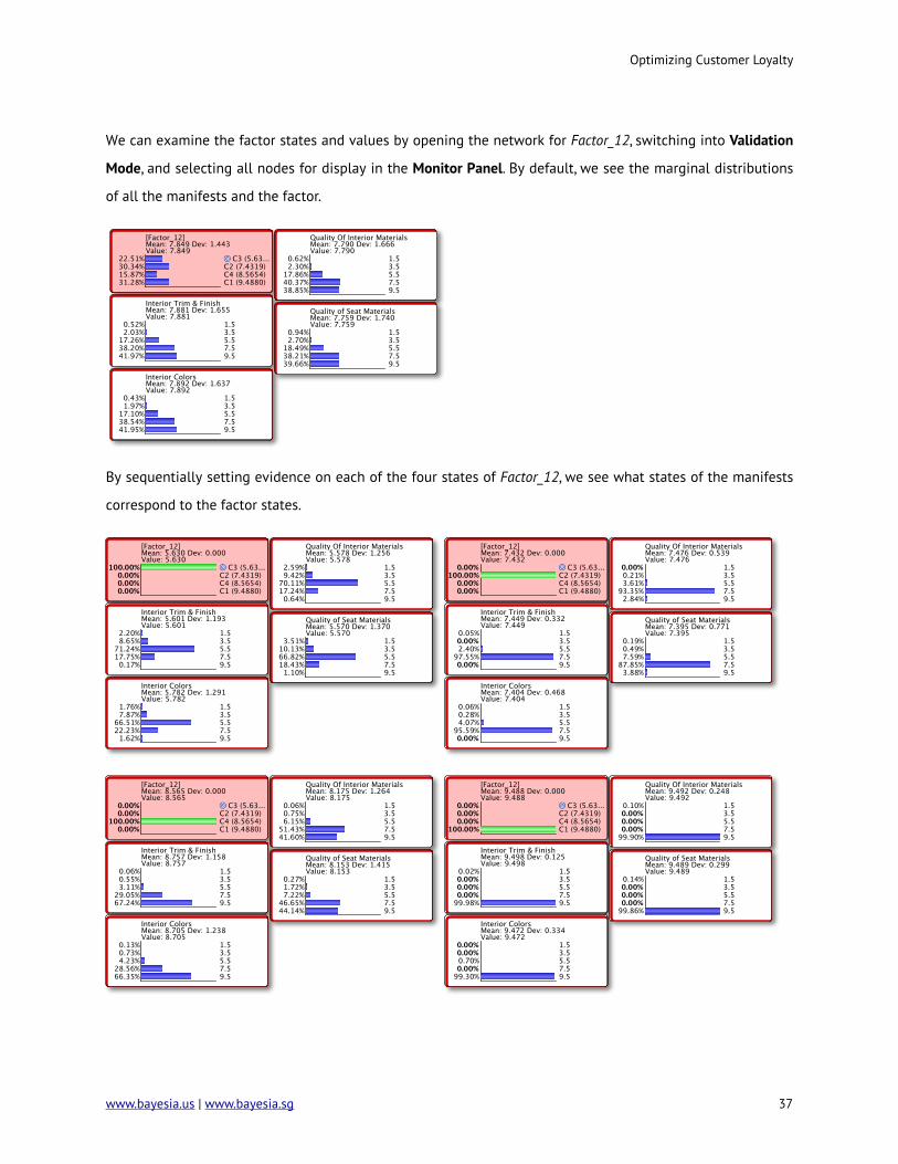
We can examine the factor states and values by opening the network for Factor_12, switching into Validation

Mode, and selecting all nodes for display in the Monitor Panel. By default, we see the marginal distributions

of all the manifests and the factor.

By sequentially setting evidence on each of the four states of Factor_12, we see what states of the manifests

correspond to the factor states.







Looking at these Monitors also provides some intuition regarding the values of the states of Factor_12.

BayesiaLab computes these values as the weighted average of the associated manifests’ values. As such, Fac-

tor_12 becomes a compact summary of the connected manifest nodes.

Introducing the Target Node

Now that factors have been formally introduced into the network, which each represent a major concept, we

can proceed to the next step. We will introduce the principal variable of interest in this study, Loyalty, as the

target variable.

This node was excluded earlier in the clustering process, so it would not become clustered into a factor. So,

the next step is to un-exclude this node, which we do by right-clicking the node and then selecting Proper-

ties | Exclusion (shortcut: press “X” and double-click on the node).

Also, we need to make this node the Target Node. We do this via by picking Set as Target Node from the

contextual menu. Note that the un-exclusion and the Target Node definition can be done at the same time by

pressing “T” and double-clicking on the excluded node.







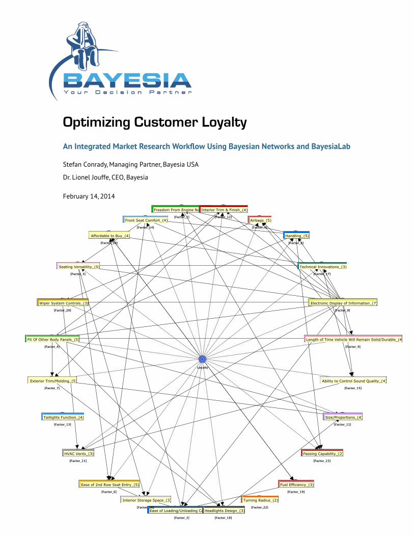
Upon introduction of the Target Node, we can interpret the status quo as the first

two layers of a hierarchical model, as illustrated below. The outer ring contains

the manifest nodes, the inner ring consists of the factors. In the middle, we have

the yet-to-be-connected Target Node.







Focusing on Factors

We could continue our analysis with this network as is, including both factors and manifest nodes. However,

for practical planning purposes, working with factors, i.e. the major concepts, is typically more relevant. Also,

removing the manifest variable will improve the expository clarity of this tutorial. Thus, we will conduct all

subsequent analyses exclusively with the factors, rather than the manifest nodes.

To delete the manifest nodes, we right-click on any one of them and then choose Select | Classes.







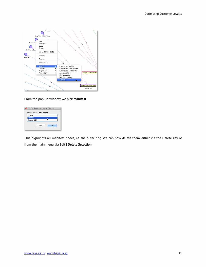
From the pop-up window, we pick Manifest.

This highlights all manifest nodes, i.e. the outer ring. We can now delete them, either via the Delete key or

from the main menu via Edit | Delete Selection.







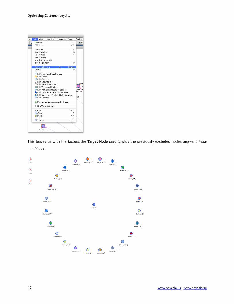
This leaves us with the factors, the Target Node Loyalty, plus the previously excluded nodes, Segment, Make

and Model.







Supervised Learning

We can now use Supervised Learning to discover the relationships between the Target Node and the factors.

We use the Augmented Markov Blanket, which is one of BayesiaLab’s Supervised Learning algorithms.

Performing this learning algorithm, using the default setting for the Structural Coefficient (SC=1), we obtain

the following network:







Structural Coefficient Analysis

In the newly-learned network, we see a total of 88 arcs connecting the 24 factor nodes and the target. Some

nodes have up to five parent nodes, which implies a 6-dimensional conditional probability table for those

nodes. Given this rather high level of complexity of the network, it is prudent to perform a Structural Coeffi-

cient Analysis: Tools | Cross Validation | Structural Coefficient Analysis.

This way we can examine, among other metrics, the data-to-structure ratio as a function of the structural

network complexity.

Once the report is presented, clicking Curve produces a kind of “scree plot”, which helps us identify a reason-

able value of the Structural Coefficient. As opposed to the scree plot that we know from Factor Analysis, here,

we read this plot from right to left.







By visual inspection of this graph, moving from right to left along the x-axis, we see an inflection point of the

curve around SC=3. Below that value, the the structural complexity is increasing faster than the data likeli-

hood. Thus, we choose SC=3 and relearn the network on that basis with the Augmented Markov Blanket algo-

rithm.

The resulting network is quite a bit simpler than before, now featuring only 65 arcs. Also, the Turning Radius

and Taillights Function factors are now no longer part of the network, which suggests that these two factors

are least relevant with regard to loyalty.







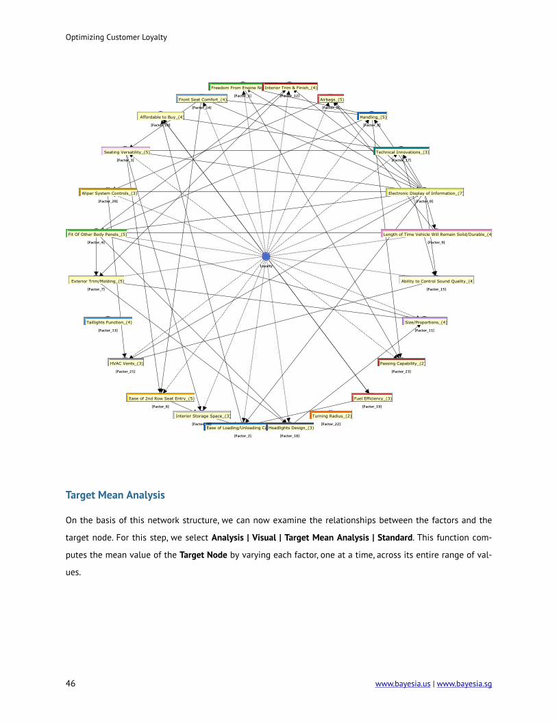
Target Mean Analysis

On the basis of this network structure, we can now examine the relationships between the factors and the

target node. For this step, we select Analysis | Visual | Target Mean Analysis | Standard. This function com-

putes the mean value of the Target Node by varying each factor, one at a time, across its entire range of val-

ues.







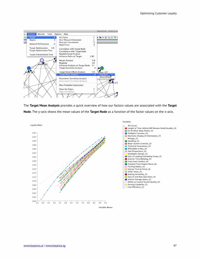
The Target Mean Analysis provides a quick overview of how our factors values are associated with the Target

Node. The y-axis shows the mean values of the Target Node as a function of the factor values on the x-axis.







This plot suggests that all the factors are approximately linearly associated with the Target Node. Further-

more, the curves appear to run almost parallel between the x-values of 7.5 and 9. As a result, it is reasonable

to formally compute “parameter estimates” for the slopes of these curves.

In BayesiaLab, this can be done by means of simulation via Analysis | Reports | Target Analysis | Total Effects

on Target. More specifically, BayesiaLab computes the derivative around the mean value of the x-range of

each factor.

The results are presented in a table. The Total Effects column shows the change of the mean value of the

Target Node, given the observation of a one-unit change in each of the factors. This value is what we com-

monly interpret as slope.







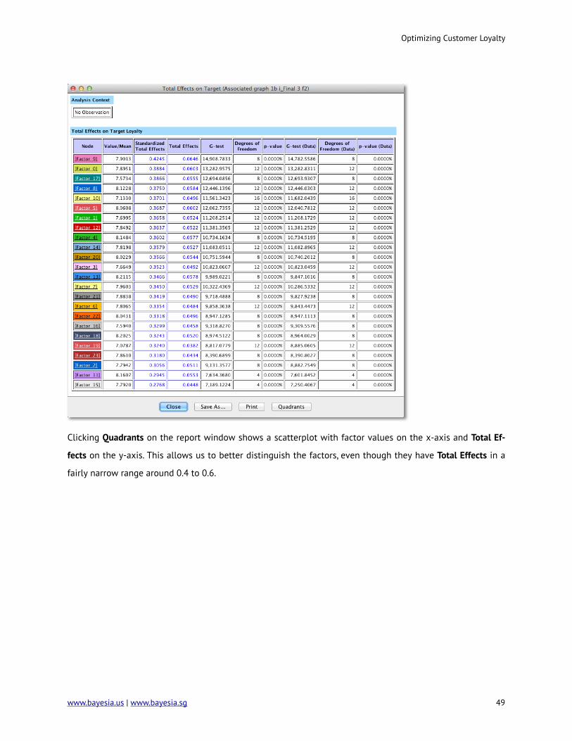
Clicking Quadrants on the report window shows a scatterplot with factor values on the x-axis and Total Ef-

fects on the y-axis. This allows us to better distinguish the factors, even though they have Total Effects in a

fairly narrow range around 0.4 to 0.6.







With the highest Total Effect, Length of Time Vehicle Will Remain Solid/Durable marks the top value on the y-

axis of the plot. The factor Fuel Efficiency marks the bottom end on both axes. The position of the Fuel Effi-

ciency factor is perhaps curious as our survey data covers 2009, when the auto industry was most severely

affected by the recession.

However, as interesting as this may seem, it is probably little practical use for planning purposes as this plot

represents a view of the entire market, across all makes and all segments. It is reasonable to assume that

effect heterogeneity exists between vehicle segments as different a Full-Size Pickups and Luxury Sedans.

Multi-Quadrant Analysis (Total Market ➔ Segment)

To study this domain at the level of vehicle segments, we could now start all over again and generate a new

network for each segment from scratch. BayesiaLab provides a convenient shortcut for the researcher by

means of Multi-Quadrant Analysis.







TotalMarket

Small Car

Full-Size Pickup

Luxury Car




…

Multi-Quadrant Anlaysis by Segment

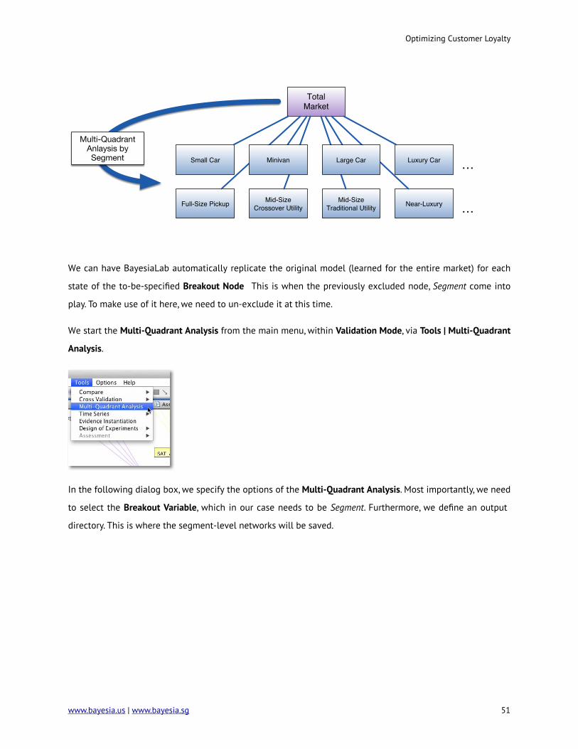
We can have BayesiaLab automatically replicate the original model (learned for the entire market) for each

state of the to-be-specified Breakout Node This is when the previously excluded node, Segment come into

play. To make use of it here, we need to un-exclude it at this time.

We start the Multi-Quadrant Analysis from the main menu, within Validation Mode, via Tools | Multi-Quadrant

Analysis.

In the following dialog box, we specify the options of the Multi-Quadrant Analysis. Most importantly, we need

to select the Breakout Variable, which in our case needs to be Segment. Furthermore, we define an output

directory. This is where the segment-level networks will be saved.







Once this process is completed, all new networks can be found in the specified directory. The file names are

created according the following syntax: Original Network File Name + _MULTI_QUADRANT_ + Breakout Variable

State.

In BayesiaLab itself, we obtain a Quadrant Plot, which shows the Mean Value of each node on the x-axis and

the Total Effect on the y-axis (even though quadrants are not explicitly shown here, we will soon explain how

a quadrant view can be helpful for interpretation).







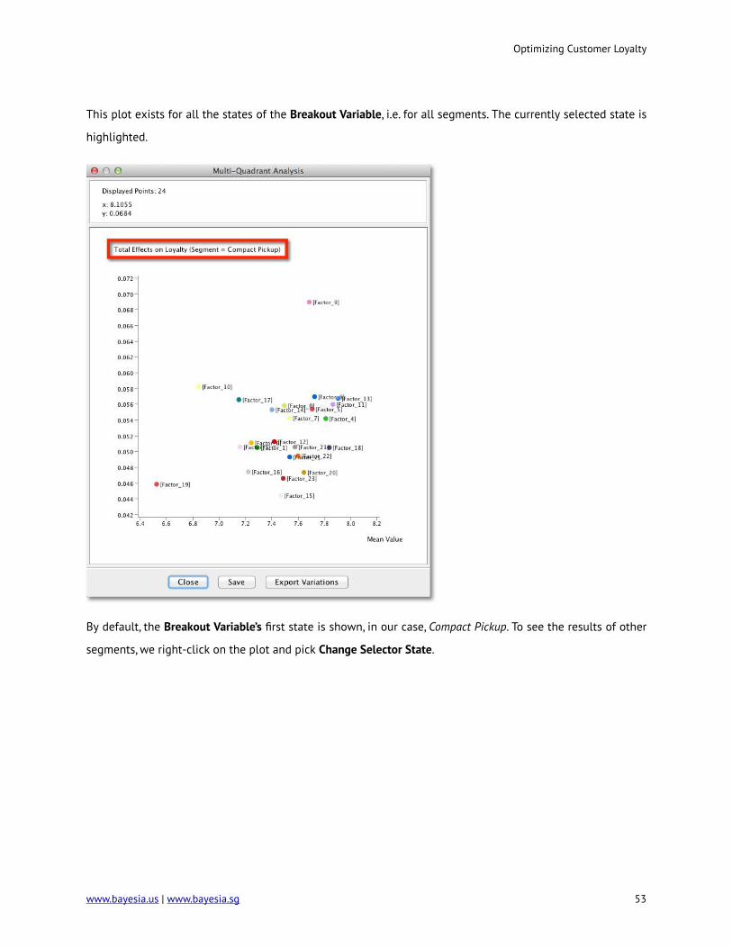
This plot exists for all the states of the Breakout Variable, i.e. for all segments. The currently selected state is

highlighted.

By default, the Breakout Variable’s first state is shown, in our case, Compact Pickup. To see the results of other

segments, we right-click on the plot and pick Change Selector State.













Full-Size Pickup Segment

For reasons explained in the introduction, we will now focus on the Full-Size Pickup segment.

This plot allows immediate interpretation. The x-axis can be represents the mean satisfaction of Full-Size

Pickup buyers with regard to the factors. The y-axis shows the Total Effect of each factor with regard to Loy-

alty. More specifically, the y-axis shows the value associated with a one-unit change of respective factor.

Casually speaking, we interpret this as the “importance” of a variable. For Full-Size Pickup, this would mean

that Ability to Control Sound Quality is fairly unimportant for Loyalty. On the other hand, even though Afford-

able to Buy rates low on the x-axis, it rates fairly high on the y-axis. This means that it is rather important for

Loyalty.

The following conceptual diagram shows a commonly-used interpretation







Q1

Q2 Q3

Q4low satisfactionlow importance

"area of opportunity" "keep up the good work"

"overkill"

Rating

Impo

rtanc

e

We should emphasize that we are interpreting factors, rather than manifest variables. Thus, the apparent “top

driver” in the Full-Size Pickup plot, Length of Time Vehicle Will Remain Solid/Durable, is actually Factor_9. Only

for convenience we applied the name of the node that most strongly contributes to this factor as node com-

ment. For reference, the manifest nodes associated with this factor are shown below.

In the Quadrant Plot, we can easily toggle between the factor name, i.e. [Factor_x], and the Node Comment via

the contextual menu.







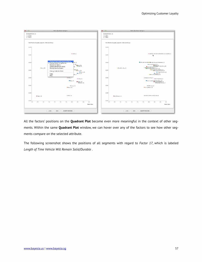
All the factors’ positions on the Quadrant Plot become even more meaningful in the context of other seg-

ments. Within the same Quadrant Plot window, we can hover over any of the factors to see how other seg-

ments compare on the selected attribute.

The following screenshot shows the positions of all segments with regard to Factor 17, which is labeled

Length of Time Vehicle Will Remain Solid/Durable .







This plot would suggest, for instance, that the Full Size Cargo Van segment has opportunities in this context.

The Premium Convertible/Roadster segment, at the other end of the spectrum, might be in the “overkill” zone.

BayesiaLab offers a convenient way to see the relative position versus the segments. From the contextual

menu, we can select Display Horizontal/Vertical Scales.







These scales show the range from the lowest to highest values. Additionally, a tick mark indicates the mean

value of the respective attribute.

In the plot below, we show the Total Effect for Length of Time Vehicle Will Remain Solid/Durable for each seg-

ment. The intersection of the of the horizontal and vertical scale indicates the position of the Full-Size Pickup

segment with regard to this variable.







This analysis can certainly help us to understand the general areas that are important for loyalty in the indi-

vidual segments. However, it does not provide any insight into the specific opportunities for individual vehi-

cle models. For this, we need to proceed to the next level of detail, i.e. the model level.

Multi-Quadrant Analysis (Segment ➔ Model)

During the earlier Multi-Quadrant Analysis, BayesiaLab generated one network file for each vehicle segment.

We now open the network for the Full-Size Pickup, the focus of this study.

Although the structure of this segment-specific network is identical to that of the original network, all the

relationship between nodes, factors and the target were re-estimated based on the subset of data corre-

sponding to the Full-Size Pickup segment.







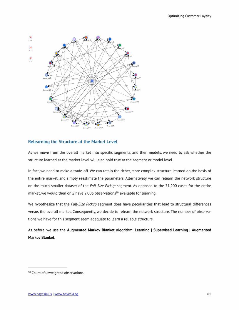
Relearning the Structure at the Market Level

As we move from the overall market into specific segments, and then models, we need to ask whether the

structure learned at the market level will also hold true at the segment or model level.

In fact, we need to make a trade-off. We can retain the richer, more complex structure learned on the basis of

the entire market, and simply reestimate the parameters. Alternatively, we can relearn the network structure

on the much smaller dataset of the Full-Size Pickup segment. As opposed to the 71,200 cases for the entire

market, we would then only have 2,003 observations10 available for learning.

We hypothesize that the Full-Size Pickup segment does have peculiarities that lead to structural differences

versus the overall market. Consequently, we decide to relearn the network structure. The number of observa-

tions we have for this segment seem adequate to learn a reliable structure.

As before, we use the Augmented Markov Blanket algorithm: Learning | Supervised Learning | Augmented

Markov Blanket.



10 Count of unweighted observations.





We may find the resulting network a bit surprising as only a single arc is discovered, namely a connection

between Affordable to Buy and Loyalty.

As we have not changed the default value, BayesiaLab used SC=1 for learning. Given the smaller amount of

data available for this segment, we need to examine whether this is the appropriate values here.







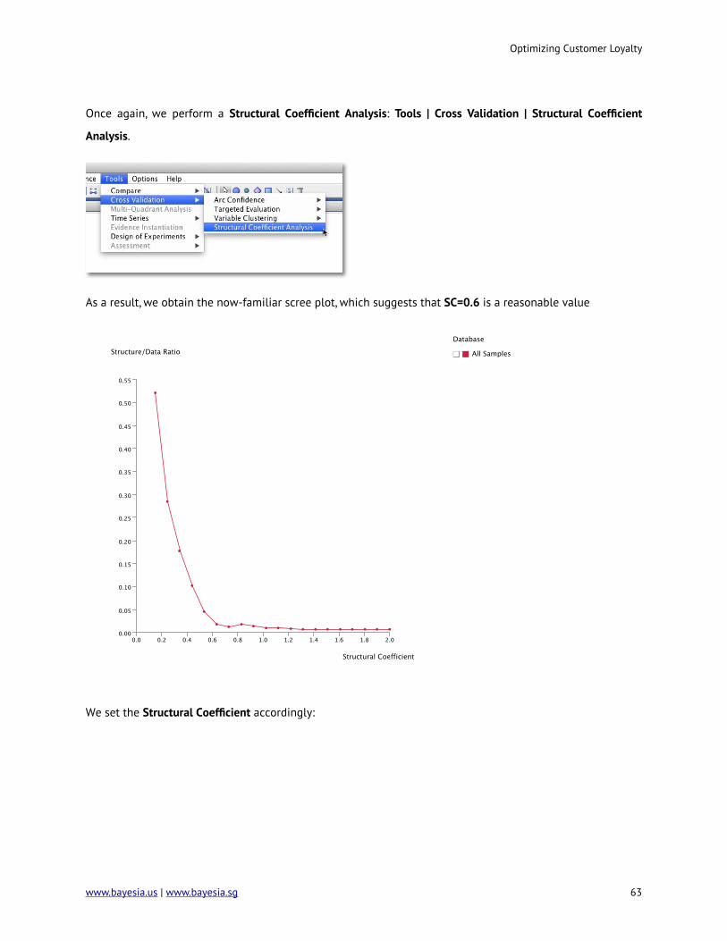
Once again, we perform a Structural Coefficient Analysis: Tools | Cross Validation | Structural Coefficient

Analysis.

As a result, we obtain the now-familiar scree plot, which suggests that SC=0.6 is a reasonable value

We set the Structural Coefficient accordingly:







Once set, we proceed to relearning the network: Learning | Supervised Learning | Augmented Markov Blanket.

The resulting network now includes 7 factors. They appear fairly intuitive for this segment.







This is not to say that other factors do not matter. Rather, with the number of available observations, none

other than the ones shown could be established with the given Structural Coefficient.

We now repeat the Target Mean Analysis: Analysis | Visual | Target Mean Analysis | Standard:







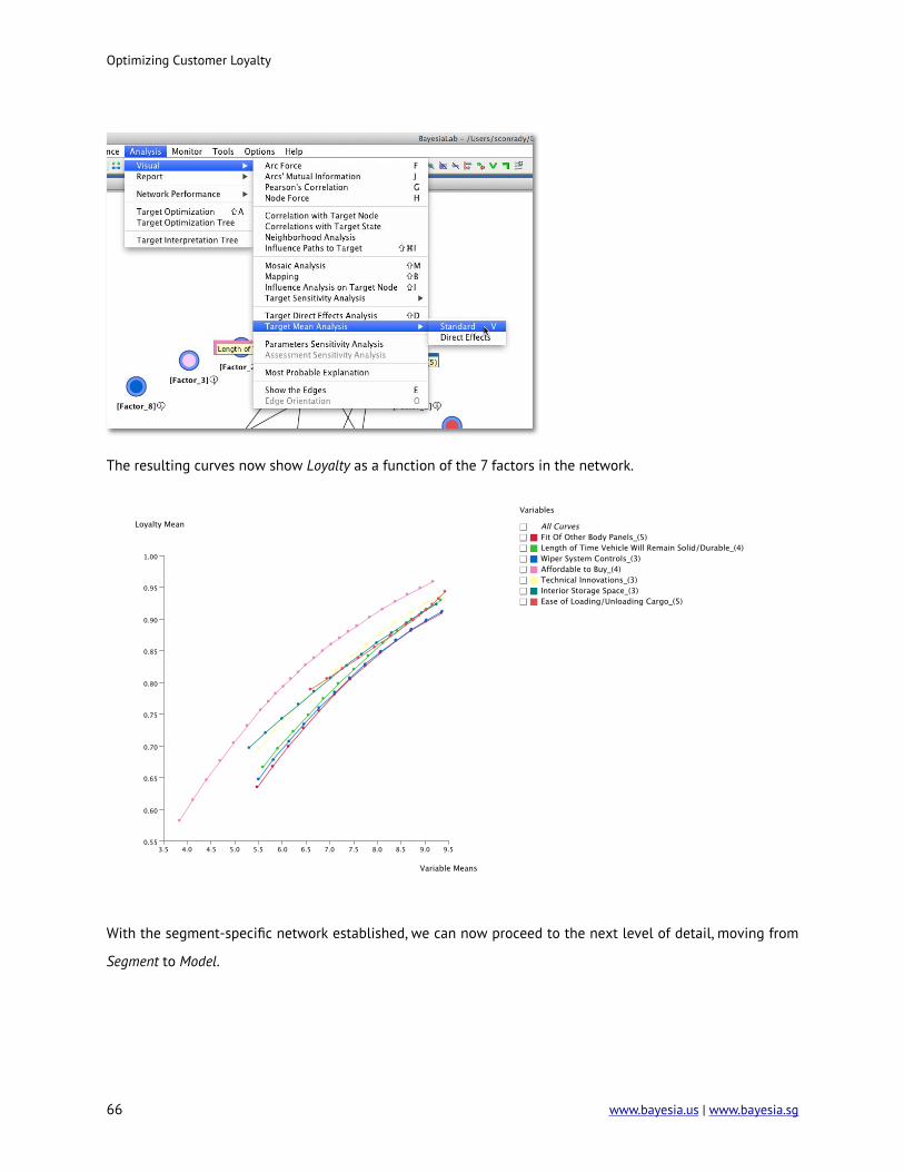
The resulting curves now show Loyalty as a function of the 7 factors in the network.

With the segment-specific network established, we can now proceed to the next level of detail, moving from

Segment to Model.







TotalMarket

Small Car

Full-Size Pickup

Luxury Car



Toyota Tundra

Nissan Titan

Ford F-150

GMC Sierra 1500

Dodge Ram

Chevrolet Silverado


…

…

Multi-Quadrant Anlaysis by

Model

For this purpose, we rerun the Multi-Quadrant Analysis and select Model as the Breakout Variable.

Furthermore, we must specify an output directory so we can subsequently analyze the model-specific net-

works.







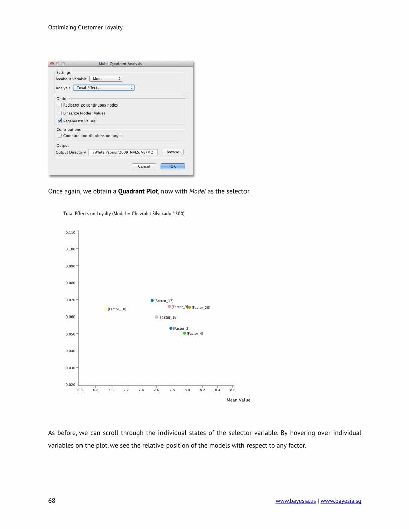
Once again, we obtain a Quadrant Plot, now with Model as the selector.

As before, we can scroll through the individual states of the selector variable. By hovering over individual

variables on the plot, we see the relative position of the models with respect to any factor.







Display Horizontal Scales/Vertical Scales, which is available from the contextual menu of the Quadrant Plot,

frames up the range of values of competitors.

Variations within the Realm of the Possible

This view is interesting on its own; however, we can more formally utilize this information. The position of

each model on the attributes’ ranges allows us to compute the “gap to best/extreme level.” This will subse-

quently become very important as we look for ways to improve brand loyalty.







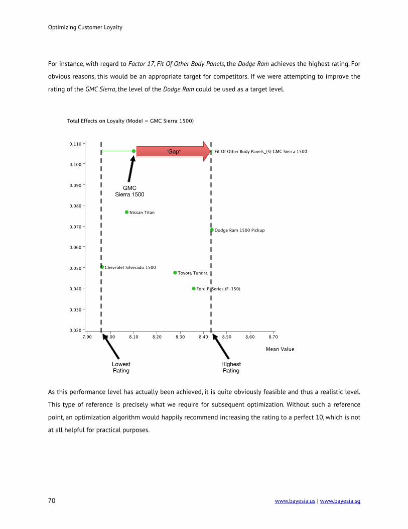
For instance, with regard to Factor 17, Fit Of Other Body Panels, the Dodge Ram achieves the highest rating. For

obvious reasons, this would be an appropriate target for competitors. If we were attempting to improve the

rating of the GMC Sierra, the level of the Dodge Ram could be used as a target level.

GMCSierra 1500

“Gap”

Lowest Rating

Highest Rating

As this performance level has actually been achieved, it is quite obviously feasible and thus a realistic level.

This type of reference is precisely what we require for subsequent optimization. Without such a reference

point, an optimization algorithm would happily recommend increasing the rating to a perfect 10, which is not

at all helpful for practical purposes.







BayesiaLab can automatically extract the delta to highest and lowest levels for each factor. In this specific

context, we call these deltas Variations. We will utilize these Variations as constraints for the optimization

algorithm.

By clicking the Export Variations button, BayesiaLab saves the Variations for the currently selected model. For

each model that we wish to optimize, we simply save this data as a text file.

Optimization

The Multi-Quadrant Analysis has generated new networks for each model, plus we have saved the associated

Variations. Thus, we have all the components necessary for optimization. For the purpose of this tutorial, we

will attempt to optimize the loyalty for the GMC Sierra.

To do so, we open the GMC Sierra-specific file generated with the most recent Multi-Quadrant Analysis.







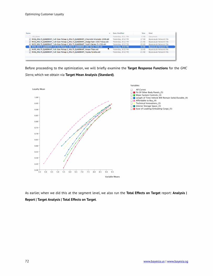
Before proceeding to the optimization, we will briefly examine the Target Response Functions for the GMC

Sierra, which we obtain via Target Mean Analysis (Standard).

As earlier, when we did this at the segment level, we also run the Total Effects on Target report: Analysis |

Report | Target Analysis | Total Effects on Target.







We obtain a report that shows the mean values of each factor, plus the corresponding Total Effects.

Here, the Quadrant Plot becomes very helpful as it shows both Value and Total Effects in a single plot.







There are many ways to interpret the above plot qualitatively. For instance, we may be tempted to look at Fit

of Other Body Panels as the top driver and suggest focusing our efforts there. Also, we might say that Technical

Innovations is fairly important, but has room for substantial improvement.

The challenge is to determine which combination of initiatives will yield the maximum improvement for loy-

alty, and what the new loyalty level would be.

This brings us back to the very purpose of this study. We start the optimization by selecting Analysis | Report |

Target Analysis | Target Dynamic Profile:







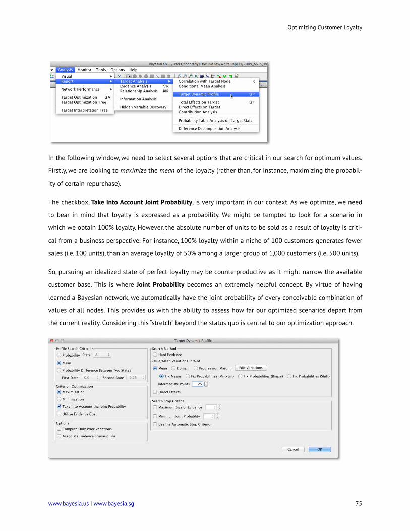
In the following window, we need to select several options that are critical in our search for optimum values.

Firstly, we are looking to maximize the mean of the loyalty (rather than, for instance, maximizing the probabil-

ity of certain repurchase).

The checkbox, Take Into Account Joint Probability, is very important in our context. As we optimize, we need

to bear in mind that loyalty is expressed as a probability. We might be tempted to look for a scenario in

which we obtain 100% loyalty. However, the absolute number of units to be sold as a result of loyalty is criti-

cal from a business perspective. For instance, 100% loyalty within a niche of 100 customers generates fewer

sales (i.e. 100 units), than an average loyalty of 50% among a larger group of 1,000 customers (i.e. 500 units).

So, pursuing an idealized state of perfect loyalty may be counterproductive as it might narrow the available

customer base. This is where Joint Probability becomes an extremely helpful concept. By virtue of having

learned a Bayesian network, we automatically have the joint probability of every conceivable combination of

values of all nodes. This provides us with the ability to assess how far our optimized scenarios depart from

the current reality. Considering this “stretch” beyond the status quo is central to our optimization approach.







The second “reality check” relates to the variations, which we discussed earlier. By default, the Variation Editor

is set to ±100%. This is what we see when we first open it.

Now we re-introduce the variations we obtained earlier. By clicking Import, we can select the previously-

saved file with the Variations for the GMC Sierra.

With the Variations loaded, we see the ranges within which the optimization value can search for the optimal

combination of values.







Clicking OK immediately starts the optimization routine. Given the small size of the network, the optimization

report pops up within seconds.

For a more detailed explanation, we save this report as an HTML file, which we can then open in Excel for

further annotation. This file keeps all the formatting, including color-coding, of the on-screen report.







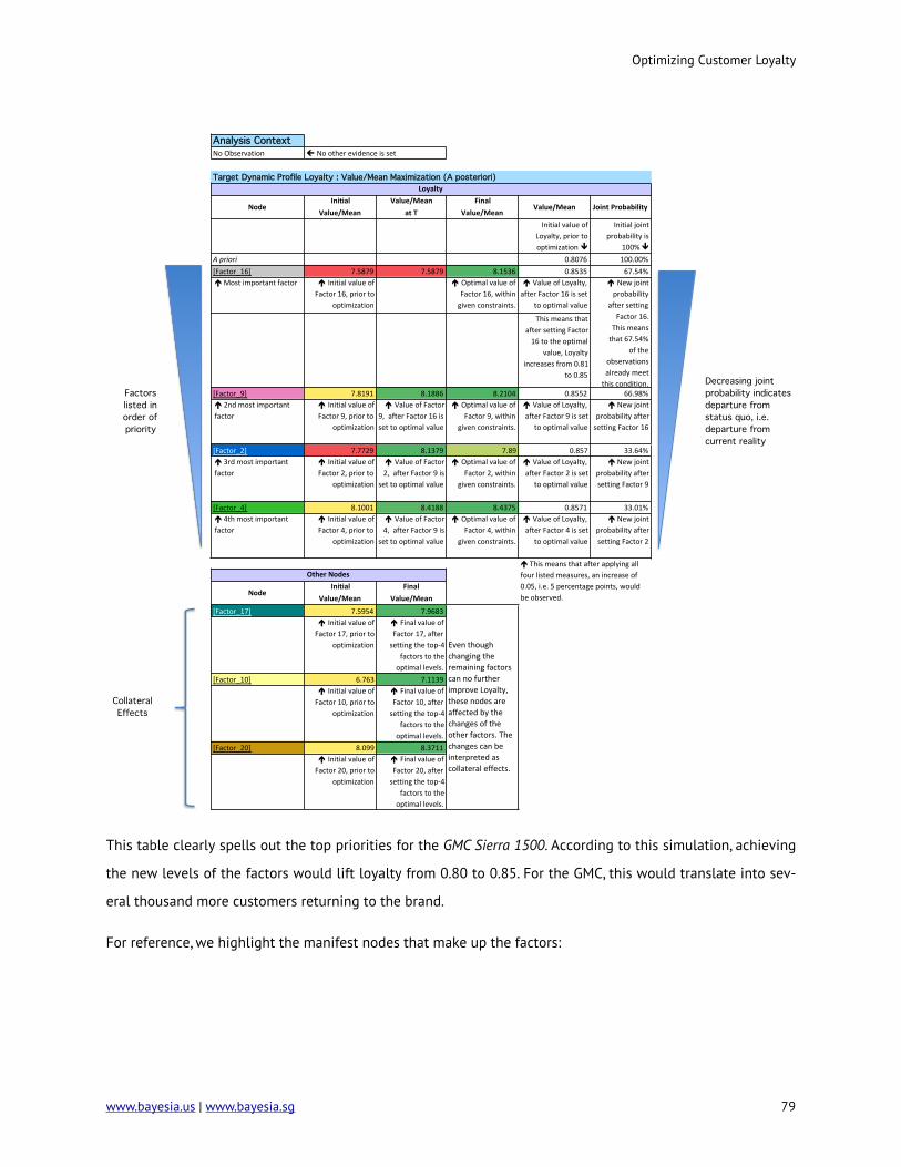
Recommendation for GMC Sierra 1500

The above report presents the results in a highly-condensed format. It will be helpful to dissect this table cell

by cell. To properly interpret this table, it should be read line-by-line, top-down.







Analysis ContextNo#Observation

Initial Value/Mean FinalValue/Mean at-T Value/Mean

#Initial#value#of#Loyalty,#prior#to#optimization#!

#Initial#joint#probability#is#

100%#!A"priori 0.8076 100.00%[Factor_16] 7.5879 7.5879 8.1536 0.8535 67.54%"#Most#important#factor #" #Initial#value#of#

Factor#16,#prior#to#optimization

#" #Optimal#value#of#Factor#16,#within#given#constraints.

#" #Value#of#Loyalty,#after#Factor#16#is#set#

to#optimal#value

This#means#that#after#setting#Factor#16#to#the#optimal#

value,#Loyalty#increases#from#0.81#

to#0.85

[Factor_9] 7.8191 8.1886 8.2104 0.8552 66.98%"#2nd#most#important#factor

#" #Initial#value#of#Factor#9,#prior#to#

optimization

#" #Value#of#Factor#9,##after#Factor#16#is#set#to#optimal#value

#" #Optimal#value#of#Factor#9,#within#

given#constraints.


to#optimal#value

"#New#joint#probability#after#setting#Factor#16

[Factor_2] 7.7729 8.1379 7.89 0.857 33.64%"#3rd#most#important#factor


optimization

#" #Value#of#Factor#2,##after#Factor#9#is#

set#to#optimal#value


given#constraints.


to#optimal#value


[Factor_4] 8.1001 8.4188 8.4375 0.8571 33.01%"#4th#most#important#factor


optimization

#" #Value#of#Factor#4,##after#Factor#9#is#

set#to#optimal#value


given#constraints.


to#optimal#value


Initial FinalValue/Mean Value/Mean

[Factor_17] 7.5954 7.9683#" #Initial#value#of#Factor#17,#prior#to#

optimization

#" #Final#value#of#Factor#17,#after#setting#the#topQ4#

factors#to#the#optimal#levels.


optimization




optimization



Decreasing joint probability indicates departure from status quo, i.e. departure from current reality

Factors listed in order of priority

Collateral Effects

"#This#means#that#after#applying#all#four#listed#measures,#an#increase#of#0.05,#i.e.#5#percentage#points,#would#be#observed.

##No#other#evidence#is#set

Target Dynamic Profile Loyalty : Value/Mean Maximization (A posteriori)

Even#though#changing#the#remaining#factors#can#no#further#improve#Loyalty,#these#nodes#are#affected#by#the#changes#of#the#other#factors.#The#changes#can#be#interpreted#as#collateral#effects.

#" #New#joint#probability#

after#setting#Factor#16.#

This#means#that#67.54%#

of#the#observations#already#meet#this#condition.

Loyalty

Node Value/Mean Joint-Probability

Other-Nodes

Node

This table clearly spells out the top priorities for the GMC Sierra 1500. According to this simulation, achieving

the new levels of the factors would lift loyalty from 0.80 to 0.85. For the GMC, this would translate into sev-

eral thousand more customers returning to the brand.

For reference, we highlight the manifest nodes that make up the factors:







Given that the earlier Multi-Quadrant Analysis generated networks for all models in this segment, we could

now repeat the optimization for any of the other models within minutes.

SummaryBayesian networks and BayesiaLab make it possible to identify relevant drivers from previously-

indistinguishable product ratings in survey data. BayesiaLab can perform optimization on that basis and im-

mediately establish priorities. With this approach, market researchers can—quickly and transparently— gener-

ate clear recommendations for decision makers.







Appendix

Variables

Select Variables from the 2009 Strategic Vision New Vehicle Experience Survey (NVES)

Combined Base Weight

Segment

Make

Model

Loyalty

Safety Features

Front Visibility – Driver

Rear Visibility – Driver

Braking

Headlights Function

Taillights Function

Turn Signal Function

Airbags

Bumpers

Solid Vehicle Construction

Length of Time Vehicle Will Remain Solid/

Durable

Freedom From Electrical Problems

Ground Clearance

Riding Comfort

Maneuverability

Turning Radius

Road Holding Ability

Handling

Steering Feedback

Acceleration From Stop

Passing Capability

Lines/Flow of the Vehicle

Appearance Of Paint Job

Size/Proportions

Side Mirrors

Appearance of Wheels & Rims

Appearance of Tires

Exterior Trim/Molding

Door Handles – Exterior

Badging (Exterior logos/identifiers)

Exterior Color

Headlights Design

Taillights Design

Sunroof

Interior Colors

Interior Trim & Finish

Body Workmanship

Fit Of Doors

Fit Of Other Body Panels

Doors/Trunk/Hatch Shutting

Wiper Performance (front/rear)

Quality Of Interior Materials

Instrument Cluster Gauges

Door Handles – Interior

Interior Lighting

Quality of Seat Materials

Freedom From Squeaks And Rattles

Freedom From Engine Noise

Freedom From Road Noise

Freedom From Wind Noise

Smoothness At Idle

Smoothness Of Transmission

Window Controls

Wiper System Controls

Speed Control System

Speakers

Ability to Control Sound Quality

Sound System Controls

CD Player

Operation of HVAC Controls

HVAC Vents

Defrost/Defog

Fuel Efficiency

Emissions Control

Front Seat Roominess

2nd row Seat Roominess

Ease of Front Seat Entry

Ease of 2nd Row Seat Entry

Comfort of Seatbelts

Support of Seats

Passenger Seating Capacity

Interior Storage Space

Cargo Capacity

Cup Holders

Ease Of Trunk/Tailgate Operation

Ease of Loading/Unloading Cargo

Front Seat Comfort

2nd row Seat Comfort

Driver Seat Adjustability

Passenger Seat Adjustability

Driver Armrests

Seating Versatility

Seating Stowaway/Conversion

Placement Of Controls/Instruments

Electronic Display of Information

Ease of Reading Controls/Instruments

Usefulness of Glove Box

Usefulness of Trunk/Cargo Area

Spare Tire

Price Or Deal Offered

Future Trade-In Or Resale Value

Warranty Coverage

Technical Innovations

Level of Standard Equipment

Fuel Economy/Mileage

Economical to Own







List of Factors Classes NodesDoor Handles - InteriorEase of Reading Controls/InstrumentsElectronic Display of InformationInstrument Cluster GaugesInterior LightingPlacement Of Controls/InstrumentsSunroofFreedom From Engine NoiseFreedom From Road NoiseFreedom From Squeaks And RattlesFreedom From Wind NoiseSmoothness At IdleSmoothness Of TransmissionEase Of Trunk/Tailgate OperationEase of Loading/Unloading CargoSpare TireUsefulness of Glove BoxUsefulness of Trunk/Cargo AreaDriver ArmrestsDriver Seat AdjustabilityPassenger Seat AdjustabilitySeating Stowaway/ConversionSeating VersatilityBody WorkmanshipDoors/Trunk/Hatch ShuttingFit Of DoorsFit Of Other Body PanelsWiper Performance (front/rear)AirbagsBumpersFront Visibility - DriverRear Visibility - DriverSafety Features2nd row Seat RoominessEase of 2nd Row Seat EntryEase of Front Seat EntryFront Seat RoominessPassenger Seating CapacityAppearance of TiresAppearance of Wheels & RimsBadging (Exterior logos/identifiers)Door Handles - ExteriorExterior Trim/MoldingGround ClearanceHandlingRiding ComfortRoad Holding AbilitySteering FeedbackFreedom From Electrical ProblemsLength of Time Vehicle Will Remain Solid/DurablePrestige/Reputation of MfrSolid Vehicle ConstructionAffordable to BuyEconomical to OwnFuture Trade-In Or Resale ValuePrice Or Deal OfferedAppearance Of Paint JobLines/Flow of the VehicleSide MirrorsSize/ProportionsInterior ColorsInterior Trim & FinishQuality Of Interior MaterialsQuality of Seat MaterialsBrakingHeadlights FunctionTaillights FunctionTurn Signal Function2nd row Seat ComfortComfort of SeatbeltsFront Seat ComfortSupport of SeatsAbility to Control Sound QualityCD PlayerSound System ControlsSpeakersCargo CapacityCup HoldersInterior Storage SpaceLevel of Standard EquipmentTechnical InnovationsWarranty CoverageExterior ColorHeadlights DesignTaillights DesignEmissions ControlFuel Economy/MileageFuel EfficiencySpeed Control SystemWindow ControlsWiper System ControlsDefrost/DefogHVAC VentsOperation of HVAC ControlsManeuverabilityTurning RadiusAcceleration From StopPassing Capability

[Factor_18]

[Factor_19]

[Factor_20]

[Factor_21]

[Factor_22]

[Factor_23]

[Factor_12]

[Factor_13]

[Factor_14]

[Factor_15]

[Factor_16]

[Factor_17]

[Factor_6]

[Factor_7]

[Factor_8]

[Factor_9]

[Factor_10]

[Factor_11]

[Factor_0]

[Factor_1]

[Factor_2]

[Factor_3]

[Factor_4]

[Factor_5]







Contact Information

Bayesia USA

312 Hamlet’s End Way

Franklin, TN 37067

USA

Phone: +1 888-386-8383

[email protected]

www.bayesia.us

Bayesia Singapore Pte. Ltd.

20 Cecil Street

#14-01, Equity Plaza

Singapore 049705

Phone: +65 3158 2690

[email protected]

www.bayesia.sg

Bayesia S.A.S.

6, rue Léonard de Vinci

BP 119

53001 Laval Cedex

France

Phone: +33(0)2 43 49 75 69

[email protected]

www.bayesia.com

Copyright

© 2014 Bayesia USA, Bayesia S.A.S. and Bayesia Singapore Pte. Ltd. All rights reserved.



mailto:[email protected]










http://www.bayesia.com

http://www.bayesia.com





Loyalty_Driver_Analysis_V13b

Documents

bayesian networks

market level

multilevel analysis

segment level

overall market

loyalty drivers

product planning priorities

customers satisfaction