Lower tropospheric ozone over India and its linkage to the ...

Atmos. Chem. Phys., 18, 3101–3118, 2018https://doi.org/10.5194/acp-18-3101-2018© Author(s) 2018. This work is distributed underthe Creative Commons Attribution 4.0 License.

Lower tropospheric ozone over India and its linkageto the South Asian monsoonXiao Lu1,2, Lin Zhang1, Xiong Liu3, Meng Gao2, Yuanhong Zhao1, and Jingyuan Shao1

1Laboratory for Climate and Ocean-Atmosphere Studies, Department of Atmospheric and Oceanic Sciences,School of Physics, Peking University, Beijing 100871, China2School of Engineering and Applied Sciences, Harvard University, Cambridge, MA 02138, USA3Harvard-Smithsonian Center for Astrophysics, Cambridge, MA 02138, USA

Correspondence: Lin Zhang ([email protected])

Received: 30 September 2017 – Discussion started: 18 October 2017Revised: 31 January 2018 – Accepted: 5 February 2018 – Published: 5 March 2018

Abstract. Lower tropospheric (surface to 600 hPa) ozoneover India poses serious risks to both human health andcrops, and potentially affects global ozone distributionthrough frequent deep convection in tropical regions. Ourcurrent understanding of the processes controlling seasonaland long-term variations in lower tropospheric ozone overthis region is rather limited due to spatially and tempo-rally sparse observations. Here we present an integratedprocess analysis of the seasonal cycle, interannual variabil-ity, and long-term trends of lower tropospheric ozone overIndia and its linkage to the South Asian monsoon usingthe Ozone Monitoring Instrument (OMI) satellite observa-tions for years 2006–2014 interpreted with a global chem-ical transport model (GEOS-Chem) simulation for 1990–2010. OMI observed lower tropospheric ozone over Indiaaveraged for 2006–2010, showing the highest concentra-tions (54.1 ppbv) in the pre-summer monsoon season (May)and the lowest concentrations (40.5 ppbv) in the summermonsoon season (August). Process analyses in GEOS-Chemshow that hot and dry meteorological conditions and activebiomass burning together contribute to 5.8 Tg more ozonebeing produced in the lower troposphere in India in Maythan January. The onset of the summer monsoon bringsozone-unfavorable meteorological conditions and strong up-ward transport, which all lead to large decreases in the lowertropospheric ozone burden. Interannually, we find that bothOMI and GEOS-Chem indicate strong positive correlations(r = 0.55–0.58) between ozone and surface temperature inpre-summer monsoon seasons, with larger correlations foundin high NOx emission regions reflecting NOx-limited pro-

duction conditions. Summer monsoon seasonal mean ozonelevels are strongly controlled by monsoon strengths. Lowerozone concentrations are found in stronger monsoon seasonsmainly due to less ozone net chemical production. Further-more, model simulations over 1990–2010 estimate a meanannual trend of 0.19± 0.07 (p value< 0.01) ppbv yr−1 in In-dian lower tropospheric ozone over this period, which aremainly driven by increases in anthropogenic emissions witha small contribution (about 7 %) from global methane con-centration increases.

1 Introduction

Ozone in the lower troposphere is a harmful air pollutant forboth humans and the ecosystem (Monks et al., 2015), andplays a central role in atmospheric chemistry as the majorsource of hydroxyl radicals (OH) (Jacob, 2000). It is alsoa short-lived greenhouse gas with a global mean radiativeforcing of 0.40 (0.20–0.60) W m−2 since the preindustrial era(Myhre et al., 2013; Stevenson et al., 2013). Troposphericozone is produced by sunlight-driven photochemical oxida-tion of carbon monoxide (CO) and hydrocarbons in the pres-ence of nitrogen oxides (NOx ≡NO+NO2). These ozoneprecursors are released not only from anthropogenic sourcessuch as industry and transportation, but also from a num-ber of climate-sensitive natural sources such as lightning,biomass burning, and biogenic emissions. It is also trans-ported from the stratosphere (about 550 Tg yr−1 or 10 % ofchemical production in the troposphere) (Stohl et al., 2003;

Published by Copernicus Publications on behalf of the European Geosciences Union.

3102 X. Lu et al.: Lower tropospheric ozone over India

Stevenson et al., 2006). Tropospheric ozone burden (present-day 337± 23 Tg) has enhanced 43 % since the preindustrialera due to rapid industrialization (Young et al., 2013). Zhanget al. (2016) recently revealed that increases in the tropo-spheric ozone burden over the past 30 years were dominatedby the equatorward redistribution of anthropogenic emis-sions to developing regions such as East and South Asia, in-creasing the interest in ozone pollution over those regions.

Unlike developed regions such as Europe and eastern US,where anthropogenic emission reductions have led to surfaceozone levels flatten or decrease since 1990s (Parrish et al.,2012; Cooper et al., 2012; Oltmans et al., 2013; Strode et al.,2015; Lin et al., 2017), developing countries such as Chinaand India have been experiencing anthropogenic emissionrises and ozone enhancements (Xu et al., 2008; Cooper etal., 2014; Sun et al., 2016; Wang et al., 2017). Recent stud-ies have shown that NOx emissions in China have been de-creasing since 2012 due to stringent air pollution controls(Krotkov et al., 2016; Liu et al., 2017). However, air qual-ity in India is continuously deteriorating as indicated by in-creasing NO2 columns observed by satellite (Krotkov et al.,2016; Geddes et al., 2016), and may become worse in thenear future considering projected trends in population andthe associated anthropogenic emissions (Ghude et al., 2016).Exposure to ozone pollution in India is estimated to havecaused 12 000 premature deaths in 2011 due to chronic ob-structive pulmonary disease (Ghude et al., 2016), and up to a36 % loss of wheat and other crop productions (Ramanathanet al., 2014; Sinha et al., 2015). In addition, frequent deepconvection in tropical Asia allows the uplifted pollutants toinfluence global ozone distribution (Lelieveld et al., 2001;Sahu et al., 2006; Beig and Brasseur, 2006; Park et al., 2007;Lawrence and Lelieveld, 2010; Srivastava et al., 2012a; Lalet al., 2013). A better understanding of the processes con-trolling lower tropospheric ozone over India thus becomesimportant to address its local and global environmental ef-fects.

Distinct seasonal transitions in prevailing wind and rain-fall associated with the monsoon circulation result in uniqueozone variations in South and East Asia. Winter monsoonprevails in October to March and brings dry and cool weatherconditions. With the onset of South Asian (East Asian) sum-mer monsoon in May, stronger westerlies (southerlies) bringmarine air from Arabian Sea (western Pacific) to the In-dian subcontinent (East Asia), leading to significant enhance-ments of cloud fractions and rainfall (Wang and LinHo,2002; Ding and Chan, 2005). Decreases of troposphericozone with the summer monsoon in South and East Asia havebeen reported from surface (Lal et al., 2000; Naja and Lal,2002; Naja et al., 2003; Beig et al., 2007; Reddy et al., 2008;Wang et al., 2009; Kumar et al., 2010; Ding et al., 2013; Houet al., 2015), ozonesonde (Zhou et al., 2013; Lal et al., 2014;Ojha et al., 2014; Sahu et al., 2014), aircraft measurements(Bhattacharjee et al., 2015; Ding et al., 2008; Srivastava etal., 2015; Ojha et al., 2016), and satellite observations (Liu

et al., 2009; Dufour et al., 2010; Safieddine et al., 2016). Anumber of modeling studies attribute the summertime ozoneminimum over India to transport of clean marine air (Lal etal., 2014; Sahu et al., 2014) or reduced ozone photochemicalproduction (Roy et al., 2008; Kumar et al., 2012). This sea-sonality is in contrast to that at mid-latitudes where surfaceozone levels are usually higher in spring and summer dueto stronger stratosphere-to-troposphere transport and photo-chemistry (Parrish et al., 2013; Cooper et al., 2014).

Most of the abovementioned studies used individualground-based observations or regional chemistry models tostudy seasonal or short-term interannual (up to 5 years) vari-ability of tropospheric ozone in India. Long-term ground-based ozone observations are extremely scarce in South Asia(Cooper et al., 2014). We also lack a comprehensive analy-sis of the spatiotemporal distribution of lower troposphericozone at a domestic scale in India. In particular, key pro-cesses that influence the tropospheric ozone budget over In-dia have not been analyzed and quantified. In this study, wepresent an integrated analysis of the processes controllinglower tropospheric (surface to 600 hPa) ozone concentrationsover the terrestrial land of India and their linkage to the SouthAsian monsoon. Satellite observations from the Ozone Mon-itoring Instrument (OMI) over 2006–2014 and simulationswith the GEOS-Chem chemical transport model (CTM) for1990–2010 are used to analyze the spatial, seasonal, and in-terannual variability of lower tropospheric ozone pollutionover India, before and during the South Asian summer mon-soon. We will further examine the potential drivers of long-term trends in lower tropospheric ozone over India.

2 Observations and model description

2.1 OMI satellite observations

The OMI instrument is onboard the NASA Earth Observ-ing System (EOS) Aura satellite launched in July 2004 withan ascending equator crossing time of ∼ 13:45 LT (localtime) (Schoeberl et al., 2006). OMI is a nadir-viewing in-strument that measures backscattered solar radiation in the0.27–0.5 µm wavelength range with a spectral resolution of0.42–0.63 nm (Levelt et al., 2006). Its nadir footprint has aspatial resolution of 13× 24 km2 with near-daily global cov-erage achieved by a wide view field of 114◦ and a 2600 kmwide swath.

We use the OMI PROFOZ ozone profile retrievals devel-oped by Liu et al. (2010) based on the optimal estimationmethod (Rodgers, 2000). Details of the PROFOZ producthave been given in Liu et al. (2010) and Kim et al. (2013),and were recently comprehensively validated by Huang etal. (2017, 2018). This OMI ozone profile algorithm retrievespartial ozone columns for 24 layers with about 2.5 km thick-ness for each layer. Here we grid the monthly mean OMI datato the 2◦× 2.5◦ horizontal resolution with focus on the spa-

Atmos. Chem. Phys., 18, 3101–3118, 2018 www.atmos-chem-phys.net/18/3101/2018/

X. Lu et al.: Lower tropospheric ozone over India 3103

tial and temporal distributions of Indian lower troposphericozone concentrations for the period of 2006–2014. Compar-isons of model simulations with OMI retrievals need to con-sider OMI a priori profiles and averaging kernel matrices asdescribed in Zhang et al. (2010). OMI a priori profiles arefrom the monthly ozone profile climatology of McPeters etal. (2007). The degrees of freedom for signals (sum of thediagonal elements of averaging kernel matrices) for OMIozone retrievals are typically 0.3–0.5 in the lower tropo-sphere over India. Previous evaluations of the OMI retrievalswith ozonesonde measurements have shown a clear improve-ment over the a priori in the lower troposphere of the tropics(30◦ S–30◦ N), and the mean retrieval biases in the tropics areless than 6 % with little seasonality (Huang et al., 2017).

2.2 GEOS-Chem simulations

We use the GEOS-Chem global CTM (v10-01; http://www.geos-chem.org) in this study. The model includes a de-tailed mechanism of ozone–NOx–VOC–aerosol troposphericchemistry (Bey et al., 2001; Park et al., 2004; Mao et al.,2010, 2013) using the chemical kinetics recommended by JetPropulsion Laboratory (JPL) and International Union of Pureand Applied Chemistry (IUPAC) (Sander et al., 2011; IU-PAC, 2013), and photolysis rates calculated by the Fast-JXscheme (Bian and Prather, 2002). Stratospheric ozone chem-istry is represented by the linearized ozone parameterization(LINOZ) (McLinden et al., 2000), and other stratosphericspecies are simulated using monthly averaged productionand loss rates archived from the Global Modeling Initiative(GMI) model (Murray et al., 2013). Physical processes suchas deposition and planetary boundary layer (PBL) mixingschemes are summarized in Table 1. The model has been ap-plied in a number of studies on global and regional tropo-spheric ozone (Wang et al., 2013; Fiore et al., 2014; Zhanget al., 2014; Lou et al., 2015; Yan et al., 2016; Zhao et al.,2017). A recent model evaluation with global troposphericozone datasets shows that GEOS-Chem (v10-01) provides animproved ozone simulation relative to previous model ver-sions (e.g., v8-01 in Zhang et al., 2010) with no significantseasonal and latitudinal biases (Hu et al., 2017).

The model is driven by the Modern Era Retrospective-analysis for Research and Application (MERRA) assimilatedmeteorological fields (Rienecker et al., 2011). For input toGEOS-Chem, we downgrade the MERRA data to 2.5◦ lon-gitude× 2◦ latitude and 47 vertical layers (extending fromsurface to 0.01 hPa) from the raw resolution of 0.667◦ longi-tude× 0.5◦ latitude and 72 layers. Emissions in the model areprocessed using the Harvard-NASA Emission Component(HEMCO) (Keller et al., 2014). Year-specific anthropogenicemissions are from the Emissions Database for Global At-mospheric Research (EDGAR v4.2 for emissions over 1990–2008, 2008 emissions are used for simulation afterwards),overwritten with regional emission inventories as summa-

rized in Table 1. Asian anthropogenic emissions are from theMIX emission inventory (Li et al., 2017).

Climate-sensitive natural ozone emissions such as bio-genic non-methane volatile organic compounds (NMVOCs)emissions, lightning NOx emissions, and soil NOx emis-sions are implemented in GEOS-Chem as summarized in Ta-ble 1. For the biomass burning emissions, we combine theAtmospheric Chemistry and Climate Model IntercomparisonProject (ACCIMP) (Lamarque et al., 2010) for 1990–1996and the Global Fire Emission Database version 3 (GFED3)(van der Werf et al., 2010) for 1997–2010. Comparison ofGFED3 and ACCMIP biomass burning CO emissions fortheir overlapping years (1997–2000) suggests that ACCMIPis 30 % higher. Here we reduce the 1990–1996 ACCMIPemissions by 30 % to reconcile the two inventories, althoughthis may lead to underestimates of biomass burning emis-sion contributions for the period. We find that biomass burn-ing emissions of CO over India (2.6 Tg a−1 (per annum)for 2006–2010) are relatively small compared with anthro-pogenic emissions (61.9 Tg a−1). As atmospheric methanehas a relatively long lifetime (about 9 years), its concentra-tions are prescribed in GEOS-Chem using year-specific mea-sured concentrations from the NOAA Global Monitoring Di-vision (GMD) (see Table 1).

We conduct a standard simulation (BASE) with year-specific assimilated meteorology and anthropogenic emis-sions from 1990 to 2010 with the initial conditions generatedby a 2-year spin-up simulation. We also conduct sensitivitysimulations by fixing one of the sources at the 1990 con-ditions, including anthropogenic emissions (FEMIS), globalmethane concentrations (FCH4), and biomass burning emis-sions (FBIOB) as summarized in Table 2. Differences be-tween the standard simulation and the sensitivity simulationsare then used to estimate influences of interannual changesin the specific source on tropospheric ozone concentrationsover India. All simulations are conducted for 1990–2010 asconstrained by the availability of MERRA meteorology andemissions.

2.3 Ozone budgets diagnosed in GEOS-Chem

We analyze processes affecting lower tropospheric ozonebudgets in each model grid including ozone chemical pro-duction and loss, horizontal and vertical transport, and drydeposition. These processes are diagnosed at every hour andaveraged to monthly mean. Net productions are calculatedas the differences between ozone chemical production andloss rates. Horizontal transport for each grid is calculatedby horizontal fluxes from or to adjacent grids. Here we de-fine transport from west to east or from south to north aspositive values. Vertical transport is estimated as the fluxat the top of the lower troposphere (600 hPa in this study)with positive values representing downward transport. TheGEOS-Chem model also includes cloud chemistry (e.g., for-mation of sulfate aerosol via aqueous-phase reactions with

www.atmos-chem-phys.net/18/3101/2018/ Atmos. Chem. Phys., 18, 3101–3118, 2018

3104 X. Lu et al.: Lower tropospheric ozone over India

Table 1. A summary of physical processes, anthropogenic and natural emissions used in GEOS-Chem.

Descriptions Sources and references

Physical processes

Wet deposition Parameterization for scavenging in both convection and large-scale precipitation for soluble gases and aerosols

Mari et al. (2000), Liu et al. (2001)and Amos et al. (2012)

Dry deposition Resistance-in-series algorithm Wesely (1989), Zhang et al. (2001)PBL mixing Non-local mixing scheme Lin and McElroy (2010)

Anthropogenic emissions

Global Emissions Database for Global Atmospheric Research(EDGAR v4.2)

http://edgar.jrc.ec.europa.eu/

East Asia and South Asia MIX emission inventory Li et al. (2017)United States Environmental Protection Agency (EPA) National Emission In-

ventory (NEI)https://www.epa.gov/air-emissions-inventories

Canada Canadian Criteria Air Contaminant http://www.ec.gc.ca/Europe European Monitoring and Evaluation Program (EMEP) http://www.emep.intMexico Big Bend Regional Aerosol and Visibility Observational study

inventory (BRAVO)Kuhns et al. (2005)

Natural sources

Biogenic emissions Model of Emissions of Gases and Aerosols from Nature(MEGAN)

Guenther et al. (2006)

Lightning (NOx) emissions Parameterization based on cloud top height, and spatially con-strained by satellite observed lightning flashes

Price and Rind (1992), Sauvage etal. (2007) and Murray et al. (2012)

Soil NOx emissions empirical parameterization of available nitrogen (N) Hudman et al. (2012)Biomass burning emissions Atmospheric Chemistry and Climate Model Intercomparison

Project (ACCIMP) for 1990–1996 and Global Fire EmissionDatabase version 3 (GFED3) for 1997–2010

Lamarque et al. (2010) and van derWerf et al. (2010)

Methane Prescribed over four latitudinal bands with year-specific mix-ing ratios constrained by measurements from the NOAA GlobalMonitoring Division (GMD). Concentration ranges over 1990–2010 are given below:90–30◦ S (1663–1732 ppbv), 30◦ S–0◦ (1666–1741 ppbv), 0–30◦ N (1733–1801 ppbv), and 30–90◦ N (1792–1855 ppbv)

ozone and H2O2) and wet deposition of soluble gases. Thetwo processes have small effects on ozone directly due to itslow solubility and thus are not diagnosed here.

3 Seasonal variation of lower troposphericozone over India

3.1 Variations of meteorology and emissions

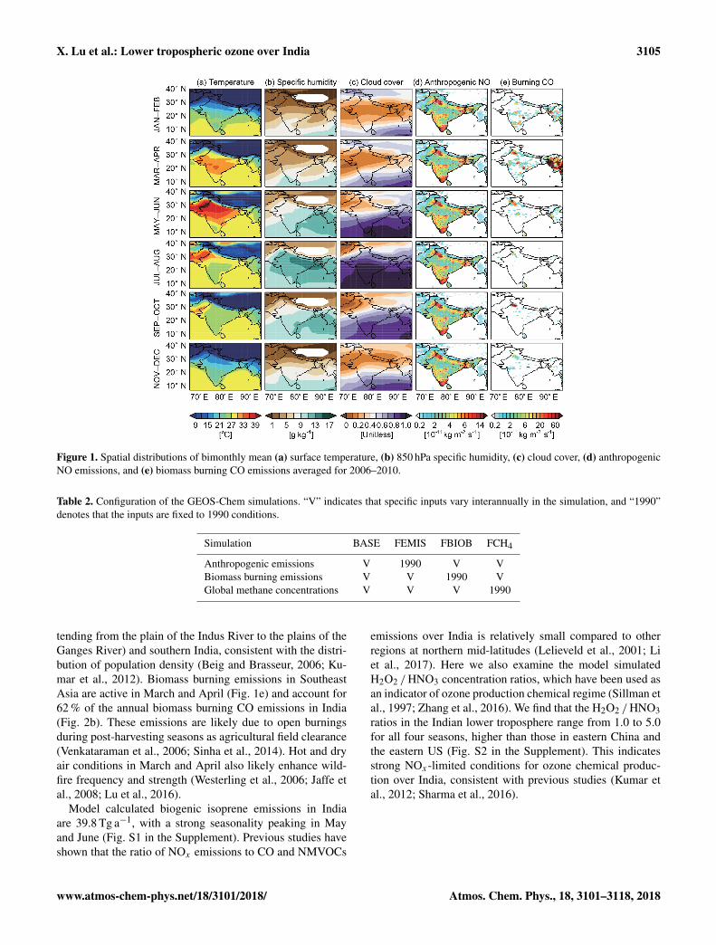
Variations in tropospheric ozone are subject to changes inprecursor emissions and meteorology conditions such as lo-cal temperature and transport pattern. Displayed in Figs. 1and 2 are the spatial and seasonal variations in MERRA me-teorological variables (surface temperature, 850 hPa specifichumidity (SPHU), and cloud cover), as well as anthropogenicNO emissions, and biomass burning CO emissions over In-dia averaged for the 5-year period (2006–2010). Meteoro-logical conditions in India have distinct seasonal variationsassociated with the monsoon onset and retreat. Temperature

increases from winter (January) to late spring (May) with in-creasing solar radiation. The onset of the summer monsoonin late May brings moist air from oceans and drives strong airconvergence and uplift over India, which lead to cloudy con-ditions, large decreases in surface temperature (about 8 ◦Cfrom May to August), and enhancements in SPHU (5 g kg−1)

(Figs. 1 and 2a). Surface temperature and SPHU becomerelatively stable with the retreat of the summer monsoon inSeptember, and then both decrease in winter when the wintermonsoon brings cold and dry air.

Figures 1 and 2b also show anthropogenic NO emissionsof 5.44 Tg a−1 (per annum) in India, with emissions in winter(December, January, and February) 3.7 % higher than sum-mer (June, July, and August) due to more active residentialheating. Anthropogenic CO and NMVOC emissions over In-dia are 61.9 and 15.5 Tg a−1, respectively, with similar sea-sonal variations as anthropogenic NO emissions (Fig. S1 inthe Supplement). Anthropogenic emissions are higher overnorthern India including the Indo-Gangetic Plain (IGP, ex-

Atmos. Chem. Phys., 18, 3101–3118, 2018 www.atmos-chem-phys.net/18/3101/2018/

X. Lu et al.: Lower tropospheric ozone over India 3105

Figure 1. Spatial distributions of bimonthly mean (a) surface temperature, (b) 850 hPa specific humidity, (c) cloud cover, (d) anthropogenicNO emissions, and (e) biomass burning CO emissions averaged for 2006–2010.

Table 2. Configuration of the GEOS-Chem simulations. “V” indicates that specific inputs vary interannually in the simulation, and “1990”denotes that the inputs are fixed to 1990 conditions.

Simulation BASE FEMIS FBIOB FCH4

Anthropogenic emissions V 1990 V VBiomass burning emissions V V 1990 VGlobal methane concentrations V V V 1990

tending from the plain of the Indus River to the plains of theGanges River) and southern India, consistent with the distri-bution of population density (Beig and Brasseur, 2006; Ku-mar et al., 2012). Biomass burning emissions in SoutheastAsia are active in March and April (Fig. 1e) and account for62 % of the annual biomass burning CO emissions in India(Fig. 2b). These emissions are likely due to open burningsduring post-harvesting seasons as agricultural field clearance(Venkataraman et al., 2006; Sinha et al., 2014). Hot and dryair conditions in March and April also likely enhance wild-fire frequency and strength (Westerling et al., 2006; Jaffe etal., 2008; Lu et al., 2016).

Model calculated biogenic isoprene emissions in Indiaare 39.8 Tg a−1, with a strong seasonality peaking in Mayand June (Fig. S1 in the Supplement). Previous studies haveshown that the ratio of NOx emissions to CO and NMVOCs

emissions over India is relatively small compared to otherregions at northern mid-latitudes (Lelieveld et al., 2001; Liet al., 2017). Here we also examine the model simulatedH2O2 /HNO3 concentration ratios, which have been used asan indicator of ozone production chemical regime (Sillman etal., 1997; Zhang et al., 2016). We find that the H2O2 /HNO3ratios in the Indian lower troposphere range from 1.0 to 5.0for all four seasons, higher than those in eastern China andthe eastern US (Fig. S2 in the Supplement). This indicatesstrong NOx-limited conditions for ozone chemical produc-tion over India, consistent with previous studies (Kumar etal., 2012; Sharma et al., 2016).

www.atmos-chem-phys.net/18/3101/2018/ Atmos. Chem. Phys., 18, 3101–3118, 2018

3106 X. Lu et al.: Lower tropospheric ozone over India

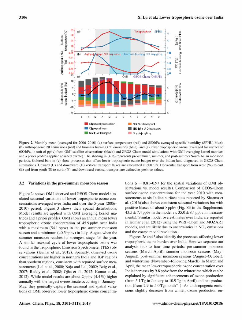
Figure 2. Monthly mean (averaged for 2006–2010) (a) surface temperature (red) and 850 hPa averaged specific humidity (SPHU, blue);(b) anthropogenic NO emissions (red) and biomass burning CO emissions (blue); and (c) lower tropospheric ozone (averaged for surface to600 hPa, in unit of ppbv) from OMI satellite observations (black) and GEOS-Chem model simulations with OMI averaging kernel matricesand a priori profiles applied (dashed purple). The shading in (a, b) represents pre-summer, summer, and post-summer South Asian monsoonperiods. Colored bars in (c) show processes that affect lower tropospheric ozone budget over the Indian land diagnosed in GEOS-Chemsimulations. Upward (U) and downward (D) vertical transport fluxes are calculated at 600 hPa. Horizontal transport from west (W) to east(E) and from south (S) to north (N), and downward vertical transport are defined as positive values.

3.2 Variations in the pre-summer monsoon season

Figure 2c shows OMI observed and GEOS-Chem model sim-ulated seasonal variations of lower tropospheric ozone con-centrations averaged over India and over the 5-year (2006–2010) period. Figure 3 shows their spatial distributions.Model results are applied with OMI averaging kernel ma-trices and a priori profiles. OMI shows an annual mean lowertropospheric ozone concentration of 45.9 ppbv over Indiawith a maximum (54.1 ppbv) in the pre-summer monsoonseason and a minimum (40.5 ppbv) in July–August when thesummer monsoon reaches its strongest stage for the year.A similar seasonal cycle of lower tropospheric ozone wasfound in the Tropospheric Emission Spectrometer (TES) ob-servations (Kumar et al., 2012). Spatially, observed ozoneconcentrations are higher in northern India and IGP regionsthan southern regions, consistent with reported surface mea-surements (Lal et al., 2000; Naja and Lal, 2002; Beig et al.,2007; Reddy et al., 2008; Ojha et al., 2012; Kumar et al.,2012). While model results are about 2 ppbv (4.4 %) higherannually with the largest overestimate occurring in January–May, they generally capture the seasonal and spatial varia-tions of OMI observed lower tropospheric ozone concentra-

tions (r = 0.81–0.97 for the spatial variations of OMI ob-servations vs. model results). Comparison of GEOS-Chemsurface ozone concentrations for the year 2010 with mea-surements at six Indian surface sites reported by Sharma etal. (2016) also shows consistent seasonal variations but withpositive biases of about 8 ppbv (Fig. S3 in the Supplement;43.5± 7.4 ppbv in the model vs. 35.0± 8.4 ppbv in measure-ments). Similar model overestimates over India are reportedin Kumar et al. (2012) using the WRF-Chem and MOZARTmodels, and are likely due to uncertainties in NOx emissionsand the coarse model resolution.

Figures 2c and 3 also identify the processes affecting lowertropospheric ozone burden over India. Here we separate ouranalysis into to four time periods: pre-summer monsoonseasons (March–April), summer monsoon seasons (May–August), post-summer monsoon seasons (August–October),and wintertime (November–following March). In March andApril, the mean lower tropospheric ozone concentration overIndia increases by 9.8 ppbv from the wintertime which can beexplained by significant enhancements of ozone production(from 5.1 Tg in January to 10.9 Tg in April) and net produc-tion (from 2.9 to 5.0 Tg month−1). As anthropogenic emis-sions slightly decrease from winter, ozone production en-

Atmos. Chem. Phys., 18, 3101–3118, 2018 www.atmos-chem-phys.net/18/3101/2018/

X. Lu et al.: Lower tropospheric ozone over India 3107

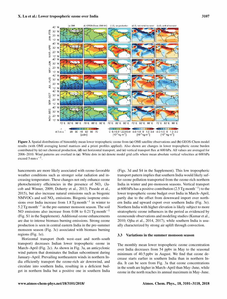
Figure 3. Spatial distributions of bimonthly mean lower tropospheric ozone from (a) OMI satellite observations and (b) GEOS-Chem modelresults (with OMI averaging kernel matrices and a priori profiles applied). Also shown are changes in lower tropospheric ozone burdencontributed by (c) net chemical production, (d) net horizontal transport, and (e) vertical transport flux at 600 hPa. All values are averaged for2006–2010. Wind patterns are overlaid in (a). White dots in (e) denote model grid cells where mean absolute vertical velocities at 600 hPaexceed 5 mm s−1.

hancements are more likely associated with ozone-favorableweather conditions such as stronger solar radiation and in-creasing temperature. These changes not only enhance ozonephotochemistry efficiencies in the presence of NOx (Ja-cob and Winner, 2009; Doherty et al., 2013; Pusede et al.,2015), but also increase natural emissions such as biogenicNMVOCs and soil NOx emissions. Biogenic isoprene emis-sions over India increase from 1.8 Tg month−1 in winter to5.2 Tg month−1 in the pre-summer monsoon season. The soilNO emissions also increase from 0.08 to 0.21 Tg month−1

(Fig. S1 in the Supplement). Additional ozone enhancementsare due to intense biomass burning emissions. Strong ozoneproduction is seen in central eastern India in the pre-summermonsoon season (Fig. 3c) associated with biomass burningregions (Fig. 1e).

Horizontal transport (both west–east and north–southtransport) decreases Indian lower tropospheric ozone inMarch–April (Fig. 2c). As shown in Fig. 3a, an anticyclonicwind pattern that dominates the Indian subcontinent duringJanuary–April. Prevailing northeastern winds in northern In-dia efficiently transport the ozone-rich air downwind, andcirculate into southern India, resulting in a deficient bud-get in northern India but a positive one in southern India

(Figs. 3d and S4 in the Supplement). This low tropospherictransport pattern implies that southern India would likely suf-fer ozone pollution transported from the ozone-rich northernIndia in winter and pre-monsoon seasons. Vertical transportat 600 hPa has a positive contribution (2.5 Tg month−1) to thelower tropospheric ozone budget over India in March–April,partly due to the offset from downward import over north-ern India and upward export over southern India (Fig. 3e).Northern India with higher elevation is likely subject to morestratospheric ozone influences in the period as evidenced byozonesonde observations and modeling studies (Kumar et al.,2010; Ojha et al., 2014, 2017), while southern India is usu-ally characterized by strong air uplift through convection.

3.3 Variations in the summer monsoon season

The monthly mean lower tropospheric ozone concentrationover India decreases from 54 ppbv in May to the seasonalminimum of 40.5 ppbv in August. We find that ozone de-crease starts earlier in southern India than in northern In-dia. It can be seen from Fig. 3a that ozone concentrationsin the south are higher in March–April than May–June, whileozone in the north reaches its annual maximum in May–June.

www.atmos-chem-phys.net/18/3101/2018/ Atmos. Chem. Phys., 18, 3101–3118, 2018

3108 X. Lu et al.: Lower tropospheric ozone over India

Vertical transport 2.5

Dry deposition -1.7 (Tg month )

Chemical production 9.9

Chemical loss -4.6

EW transport -2.9

NS transport -1.7

(a) Pre-summer monsoon seasonMarch and April

Vertical transport -2.9

Dry deposition -1.4

Chemical production 8.4

Chemical loss -5.2EW transport 0.8

(b) Summer monsoon seasonJune, July and August

Net ozone budget 1.5 NS transport -0.2 Net ozone budget -0.5

-1

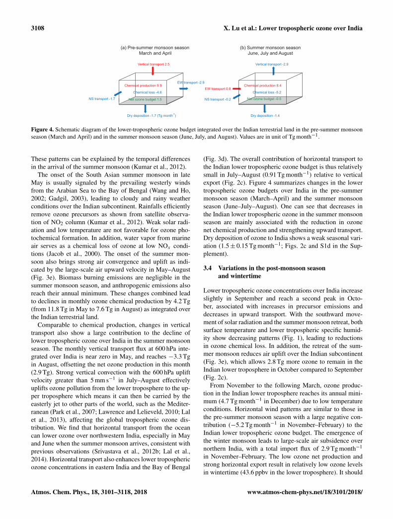
Figure 4. Schematic diagram of the lower-tropospheric ozone budget integrated over the Indian terrestrial land in the pre-summer monsoonseason (March and April) and in the summer monsoon season (June, July, and August). Values are in unit of Tg month−1.

These patterns can be explained by the temporal differencesin the arrival of the summer monsoon (Kumar et al., 2012).

The onset of the South Asian summer monsoon in lateMay is usually signaled by the prevailing westerly windsfrom the Arabian Sea to the Bay of Bengal (Wang and Ho,2002; Gadgil, 2003), leading to cloudy and rainy weatherconditions over the Indian subcontinent. Rainfalls efficientlyremove ozone precursors as shown from satellite observa-tion of NO2 column (Kumar et al., 2012). Weak solar radi-ation and low temperature are not favorable for ozone pho-tochemical formation. In addition, water vapor from marineair serves as a chemical loss of ozone at low NOx condi-tions (Jacob et al., 2000). The onset of the summer mon-soon also brings strong air convergence and uplift as indi-cated by the large-scale air upward velocity in May–August(Fig. 3e). Biomass burning emissions are negligible in thesummer monsoon season, and anthropogenic emissions alsoreach their annual minimum. These changes combined leadto declines in monthly ozone chemical production by 4.2 Tg(from 11.8 Tg in May to 7.6 Tg in August) as integrated overthe Indian terrestrial land.

Comparable to chemical production, changes in verticaltransport also show a large contribution to the decline oflower tropospheric ozone over India in the summer monsoonseason. The monthly vertical transport flux at 600 hPa inte-grated over India is near zero in May, and reaches −3.3 Tgin August, offsetting the net ozone production in this month(2.9 Tg). Strong vertical convection with the 600 hPa upliftvelocity greater than 5 mm s−1 in July–August effectivelyuplifts ozone pollution from the lower troposphere to the up-per troposphere which means it can then be carried by theeasterly jet to other parts of the world, such as the Mediter-ranean (Park et al., 2007; Lawrence and Lelieveld, 2010; Lalet al., 2013), affecting the global tropospheric ozone dis-tribution. We find that horizontal transport from the oceancan lower ozone over northwestern India, especially in Mayand June when the summer monsoon arrives, consistent withprevious observations (Srivastava et al., 2012b; Lal et al.,2014). Horizontal transport also enhances lower troposphericozone concentrations in eastern India and the Bay of Bengal

(Fig. 3d). The overall contribution of horizontal transport tothe Indian lower tropospheric ozone budget is thus relativelysmall in July–August (0.91 Tg month−1) relative to verticalexport (Fig. 2c). Figure 4 summarizes changes in the lowertropospheric ozone budgets over India in the pre-summermonsoon season (March–April) and the summer monsoonseason (June–July–August). One can see that decreases inthe Indian lower tropospheric ozone in the summer monsoonseason are mainly associated with the reduction in ozonenet chemical production and strengthening upward transport.Dry deposition of ozone to India shows a weak seasonal vari-ation (1.5± 0.15 Tg month−1; Figs. 2c and S1d in the Sup-plement).

3.4 Variations in the post-monsoon seasonand wintertime

Lower tropospheric ozone concentrations over India increaseslightly in September and reach a second peak in Octo-ber, associated with increases in precursor emissions anddecreases in upward transport. With the southward move-ment of solar radiation and the summer monsoon retreat, bothsurface temperature and lower tropospheric specific humid-ity show decreasing patterns (Fig. 1), leading to reductionsin ozone chemical loss. In addition, the retreat of the sum-mer monsoon reduces air uplift over the Indian subcontinent(Fig. 3e), which allows 2.8 Tg more ozone to remain in theIndian lower troposphere in October compared to September(Fig. 2c).

From November to the following March, ozone produc-tion in the Indian lower troposphere reaches its annual mini-mum (4.7 Tg month−1 in December) due to low temperatureconditions. Horizontal wind patterns are similar to those inthe pre-summer monsoon season with a large negative con-tribution (−5.2 Tg month−1 in November–February) to theIndian lower tropospheric ozone budget. The emergence ofthe winter monsoon leads to large-scale air subsidence overnorthern India, with a total import flux of 2.9 Tg month−1

in November–February. The low ozone net production andstrong horizontal export result in relatively low ozone levelsin wintertime (43.6 ppbv in the lower troposphere). It should

Atmos. Chem. Phys., 18, 3101–3118, 2018 www.atmos-chem-phys.net/18/3101/2018/

X. Lu et al.: Lower tropospheric ozone over India 3109

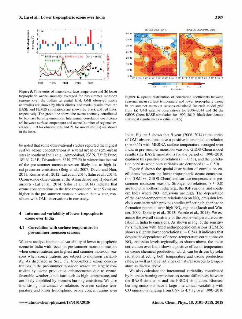
Figure 5. Time series of mean (a) surface temperature and (b) lowertropospheric ozone anomaly averaged for pre-summer monsoonseasons over the Indian terrestrial land. OMI observed ozoneanomalies are shown by black circles, and model results from theBASE and FEMIS simulations are shown by black and red lines,respectively. The green line shows the ozone anomaly contributedby biomass burning emissions. Interannual correlation coefficients(r) between surface temperature and ozone (number of regional av-erages n= 9 for observations and 21 for model results) are shownin the inset.

be noted that some observational studies reported the highestsurface ozone concentrations at several urban or semi-urbansites in southern India (e.g., Ahmedabad, 23◦ N, 73◦ E; Pune,18◦ N, 74◦ E; Trivandrum, 8◦ N, 77◦ E) in wintertime insteadof the pre-summer monsoon season likely due to high lo-cal precursor emissions (Beig et al., 2007; David and Nair,2011; Kumar et al., 2012; Lal et al., 2014; Sahu et al., 2014).Ozonesonde observations at the Ahmedabad and Hyderabadairports (Lal et al., 2014; Sahu et al., 2014) indicate thatozone concentrations in the free troposphere (near 5 km) arehigher in the pre-summer monsoon season than winter, con-sistent with OMI observations in our study.

4 Interannual variability of lower troposphericozone over India

4.1 Correlation with surface temperature inpre-summer monsoon seasons

We now analyze interannual variability of lower troposphericozone in India with focus on pre-summer monsoon seasonswhen concentrations are highest and summer monsoon sea-sons when concentrations are subject to monsoon variabil-ity. As discussed in Sect. 3.2, tropospheric ozone concen-trations in the pre-summer monsoon season are largely con-trolled by ozone production enhancements due to ozone-favorable weather conditions such as high temperature, andare likely amplified by biomass burning emissions. We alsofind strong interannual correlations between surface tem-perature and lower tropospheric ozone concentrations over

65° E 70° E 75° E 80° E 85° E 90° E 95° E5° N

10° N

15° N

20° N

25° N

30° N

35° N

40° N (a) OMI (2006–2014) (b) GEOS-Chem (1990–2010)

-0.8 -0.4 0 0.4 0.8Correlation

65° E 70° E 75° E 80° E 85° E 90° E 95° E

Figure 6. Spatial distribution of correlation coefficients betweenseasonal mean surface temperature and lower tropospheric ozonein pre-summer monsoon seasons calculated for each model gridfrom (a) OMI satellite observations for 2006–2014 and (b) theGEOS-Chem BASE simulation for 1990–2010. Black dots denotestatistical significance (p value< 0.05).

India. Figure 5 shows that 9-year (2006–2014) time seriesof OMI observations have a positive interannual correlation(r = 0.55) with MERRA surface temperature averaged overIndia in pre-summer monsoon seasons. GEOS-Chem modelresults (the BASE simulation) for the period of 1990–2010captured this positive correlation (r = 0.58), and the correla-tion persists when both variables are detrended (r = 0.50).

Figure 6 shows the spatial distribution of correlation co-efficients between the lower tropospheric ozone concentra-tion (OMI vs. GEOS-Chem) and surface temperature in pre-summer monsoon seasons. Stronger correlations (r ≈ 0.8)are found in northern India (e.g., the IGP regions) and south-ern India where NOx emissions are high. The dependenceof the ozone–temperature relationship on NOx emission lev-els is consistent with previous studies reflecting higher ozoneformation potential over high NOx regions (Jacob and Win-ner, 2009; Doherty et al., 2013; Pusede et al., 2015). We ex-amine the overall sensitivity of the ozone–temperature corre-lation in India to emissions. As shown in Fig. 5, the sensitiv-ity simulation with fixed anthropogenic emissions (FEMIS)shows a slightly lower correlation (r = 0.54). It indicates thatdespite the dependence of ozone–temperature correlations onNOx emission levels regionally, as shown above, the meancorrelation over India shows a positive effect of temperatureon ozone chemical production, which can be driven by solarradiation affecting both temperature and ozone productionrates, as well as the sensitivities of natural sources to temper-ature as discuss above.

We also calculate the interannual variability contributedby biomass burning emissions as ozone differences betweenthe BASE simulation and the FBIOB simulation. Biomassburning emissions have a large interannual variability withCO emissions ranging from 0.97 to 4.7 Tg over 1990–2010

www.atmos-chem-phys.net/18/3101/2018/ Atmos. Chem. Phys., 18, 3101–3118, 2018

3110 X. Lu et al.: Lower tropospheric ozone over India

(Fig. S5 in the Supplement). As can be seen from Fig. 5, theozone interannual variability contributed by biomass burn-ing emissions is weakly correlated with the BASE lowertropospheric ozone (r = 0.29). However, they are importantin high ozone and high temperature years. In years such as1999 and 2010, biomass burning caused 1.5–2.2 ppbv higherozone, enhancing the variability of lower tropospheric ozone.This eventuality has also been noted in the western US (Jaffeet al., 2008; Lu et al., 2016) as high temperature conditionsfavored both biomass burning emissions and ozone produc-tion, and thus amplified lower tropospheric ozone concentra-tions.

4.2 Impact of monsoon strength in summermonsoon seasons

We have also shown above that lower tropospheric ozoneconcentrations over India vary relative to the onset and retreatof the South Asian summer monsoon. The interannual vari-ability of lower tropospheric ozone over India in the summermonsoon seasons (May–August) can then be affected by thestrength of the South Asian summer monsoon. To quantifythis relationship, we calculate the monsoon strength usingthe monsoon index proposed by Li and Zeng (2002) whichhas been applied to quantify impacts of the East Asian mon-soon on air pollution over China (Zhu et al., 2012; Yang et al.,2014). The monsoon index is first calculated for each modelgrid (δ(i,j)) in the Northern Hemisphere in the monthm andyear y as

δy,m (i,j)=

∥∥V 1(i,j)−V y,m (i,j)∥∥∥∥(V 1(i,j)+V 7(i,j))/2∥∥ − 2, (1)

where V represents monthly mean wind speed from theMERRA dataset, and V 1 and V 7 are climatological (1990–2010 in our study) monthly wind speed in January and July,respectively. The norm of a given variable A is defined as

‖A‖ =

(∫ ∫|A|2dS

)1/2

, (2)

where S represents the spatial area of a model grid cell.Details for the calculation of ‖A‖ are given in Li andZeng (2002) and Zhu et al. (2012). In this study, we thenaverage δ(i,j) over the region of 35–90◦ E, 5–35◦ N (Fig. S2in the Supplement) at 850 hPa and over May–August to rep-resent the South Asian summer monsoon index (SASMI).

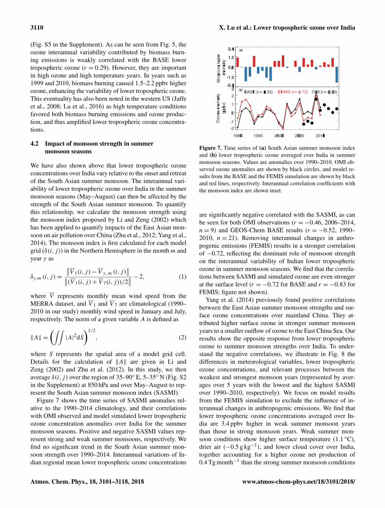
Figure 7 shows the time series of SASMI anomalies rel-ative to the 1990–2014 climatology, and their correlationswith OMI observed and model simulated lower troposphericozone concentration anomalies over India for the summermonsoon seasons. Positive and negative SASMI values rep-resent strong and weak summer monsoons, respectively. Wefind no significant trend in the South Asian summer mon-soon strength over 1990–2014. Interannual variations of In-dian regional mean lower tropospheric ozone concentrations

Figure 7. Time series of (a) South Asian summer monsoon indexand (b) lower tropospheric ozone averaged over India in summermonsoon seasons. Values are anomalies over 1990–2010. OMI ob-served ozone anomalies are shown by black circles, and model re-sults from the BASE and the FEMIS simulation are shown by blackand red lines, respectively. Interannual correlation coefficients withthe monsoon index are shown inset.

are significantly negative correlated with the SASMI, as canbe seen for both OMI observations (r =−0.46, 2006–2014,n= 9) and GEOS-Chem BASE results (r =−0.52, 1990–2010, n= 21). Removing interannual changes in anthro-pogenic emissions (FEMIS) results in a stronger correlationof −0.72, reflecting the dominant role of monsoon strengthon the interannual variability of Indian lower troposphericozone in summer monsoon seasons. We find that the correla-tions between SASMI and simulated ozone are even strongerat the surface level (r =−0.72 for BASE and r =−0.83 forFEMIS; figure not shown).

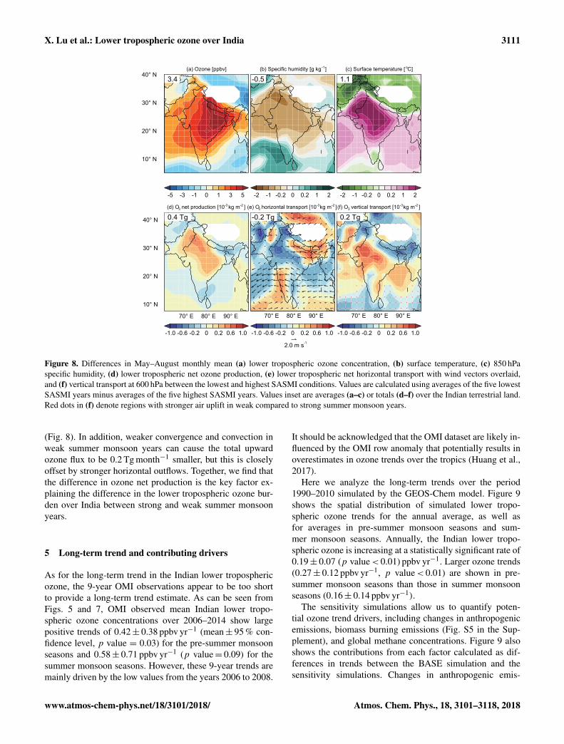
Yang et al. (2014) previously found positive correlationsbetween the East Asian summer monsoon strengths and sur-face ozone concentrations over mainland China. They at-tributed higher surface ozone in stronger summer monsoonyears to a smaller outflow of ozone to the East China Sea. Ourresults show the opposite response from lower troposphericozone to summer monsoon strengths over India. To under-stand the negative correlations, we illustrate in Fig. 8 thedifferences in meteorological variables, lower troposphericozone concentrations, and relevant processes between theweakest and strongest monsoon years (represented by aver-ages over 5 years with the lowest and the highest SASMIover 1990–2010, respectively). We focus on model resultsfrom the FEMIS simulation to exclude the influence of in-terannual changes in anthropogenic emissions. We find thatlower tropospheric ozone concentrations averaged over In-dia are 3.4 ppbv higher in weak summer monsoon yearsthan those in strong monsoon years. Weak summer mon-soon conditions show higher surface temperature (1.1 ◦C),drier air (−0.5 g kg−1), and lower cloud cover over India,together accounting for a higher ozone net production of0.4 Tg month−1 than the strong summer monsoon conditions

Atmos. Chem. Phys., 18, 3101–3118, 2018 www.atmos-chem-phys.net/18/3101/2018/

X. Lu et al.: Lower tropospheric ozone over India 3111

10° N

20° N

30° N

40° N

-5 -3 -1 0 1 3 5

(a) Ozone [ppbv]

3.4

-2 -1 -0.2 0 0.2 1 2

(b) Specific humidity [g kg-1]

-0.5

-2 -1 -0.2 0 0.2 1 2

(c) Surface temperature [ oC]

1.1

70° E 80° E 90° E

-1.0 -0.6 -0.2 0 0.2 0.6 1.0

(d) O3 net production [10-3 kg m-2 ]

0.4 Tg

2.0 m s

-1

-1.0 -0.6 -0.2 0 0.2 0.6 1.0

(e) O3 horizontal transport [10-3 kg m-2 ]

-0.2 Tg

-1.0 -0.6 -0.2 0 0.2 0.6 1.0

(f) O3 vertical transport [10-3 kg m-2 ]

0.2 Tg

-1

10° N

20° N

30° N

40° N

70° E 80° E 90° E 70° E 80° E 90° E

Figure 8. Differences in May–August monthly mean (a) lower tropospheric ozone concentration, (b) surface temperature, (c) 850 hPaspecific humidity, (d) lower tropospheric net ozone production, (e) lower tropospheric net horizontal transport with wind vectors overlaid,and (f) vertical transport at 600 hPa between the lowest and highest SASMI conditions. Values are calculated using averages of the five lowestSASMI years minus averages of the five highest SASMI years. Values inset are averages (a–c) or totals (d–f) over the Indian terrestrial land.Red dots in (f) denote regions with stronger air uplift in weak compared to strong summer monsoon years.

(Fig. 8). In addition, weaker convergence and convection inweak summer monsoon years can cause the total upwardozone flux to be 0.2 Tg month−1 smaller, but this is closelyoffset by stronger horizontal outflows. Together, we find thatthe difference in ozone net production is the key factor ex-plaining the difference in the lower tropospheric ozone bur-den over India between strong and weak summer monsoonyears.

5 Long-term trend and contributing drivers

As for the long-term trend in the Indian lower troposphericozone, the 9-year OMI observations appear to be too shortto provide a long-term trend estimate. As can be seen fromFigs. 5 and 7, OMI observed mean Indian lower tropo-spheric ozone concentrations over 2006–2014 show largepositive trends of 0.42± 0.38 ppbv yr−1 (mean± 95 % con-fidence level, p value = 0.03) for the pre-summer monsoonseasons and 0.58± 0.71 ppbv yr−1 (p value= 0.09) for thesummer monsoon seasons. However, these 9-year trends aremainly driven by the low values from the years 2006 to 2008.

It should be acknowledged that the OMI dataset are likely in-fluenced by the OMI row anomaly that potentially results inoverestimates in ozone trends over the tropics (Huang et al.,2017).

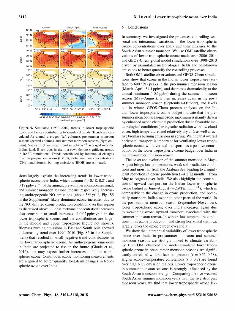
Here we analyze the long-term trends over the period1990–2010 simulated by the GEOS-Chem model. Figure 9shows the spatial distribution of simulated lower tropo-spheric ozone trends for the annual average, as well asfor averages in pre-summer monsoon seasons and sum-mer monsoon seasons. Annually, the Indian lower tropo-spheric ozone is increasing at a statistically significant rate of0.19± 0.07 (p value< 0.01) ppbv yr−1. Larger ozone trends(0.27± 0.12 ppbv yr−1, p value< 0.01) are shown in pre-summer monsoon seasons than those in summer monsoonseasons (0.16± 0.14 ppbv yr−1).

The sensitivity simulations allow us to quantify poten-tial ozone trend drivers, including changes in anthropogenicemissions, biomass burning emissions (Fig. S5 in the Sup-plement), and global methane concentrations. Figure 9 alsoshows the contributions from each factor calculated as dif-ferences in trends between the BASE simulation and thesensitivity simulations. Changes in anthropogenic emis-

www.atmos-chem-phys.net/18/3101/2018/ Atmos. Chem. Phys., 18, 3101–3118, 2018

3112 X. Lu et al.: Lower tropospheric ozone over India

Annual March–April May–August

10° N

20° N

30° N

40° N 0.19

BASE

0.27 0.16

0.18

EMIS

0.21 0.19

0.02

CH 4

0.02 0.02

70° E 80° E 90° E

-0.01

BIO

B

-0.03 -0.02

-0.32 -0.24 -0.16 -0.08 -0.02 0.02 0.08 0.16 0.24 0.32Ozone trend [ppbv year -1 ]

10° N

20° N

30° N

40° N

10° N

20° N

30° N

40° N

10° N

20° N

30° N

40° N

70° E 80° E 90° E 70° E 80° E 90° E

Figure 9. Simulated (1990–2010) trends in lower troposphericozone and factors contributing to simulated trends. Trends are cal-culated for annual averages (left column), pre-summer monsoonseasons (central column), and summer monsoon seasons (right col-umn). Values inset are mean trend in ppbv yr−1 averaged over theIndian land. Black dots in the first rows denote significant trendsin BASE simulations. Trends contributed by interannual changesin anthropogenic emissions (EMIS), global methane concentrations(CH4), and biomass burning emissions (BIOB) are estimated.

sions largely explain the increasing trends in lower tropo-spheric ozone over India, which account for 0.18, 0.21, and0.19 ppbv yr−1 of the annual, pre-summer monsoon seasonal,and summer monsoon seasonal means, respectively. Increas-ing anthropogenic NO emissions (about 3 % yr−1, Fig. S5in the Supplement) likely dominate ozone increases due tothe NOx-limited ozone production condition over this regionas discussed above. Global methane concentration increasesalso contribute to small increases of 0.02 ppbv yr−1 in thelower tropospheric ozone, and the contributions are largerin the middle and upper troposphere (figure not shown).Biomass burning emissions in East and South Asia showeda decreasing trend over 1990–2010 (Fig. S5 in the Supple-ment) that resulted in small negative trend contributions inthe lower tropospheric ozone. As anthropogenic emissionsin India are projected to rise in the future (Ghude et al.,2016), one may expect further increases in Indian tropo-spheric ozone. Continuous ozone monitoring measurementsare required to better quantify long-term changes in tropo-spheric ozone over India.

6 Conclusions

In summary, we investigated the processes controlling sea-sonal and interannual variations in the lower troposphericozone concentrations over India and their linkages to theSouth Asian summer monsoon. We use OMI satellite obser-vations of lower tropospheric ozone made over 2006–2014and GEOS-Chem global model simulations over 1990–2010driven by assimilated meteorological fields and best-knownemissions to better quantify the controlling processes.

Both OMI satellite observations and GEOS-Chem simula-tions show that ozone in the Indian lower troposphere (sur-face to 600 hPa) peaks in the pre-summer monsoon season(March–April, 54.1 ppbv), and decreases dramatically to theannual minimum (40.5 ppbv) during the summer monsoonseason (May–August). It then increases again in the post-summer monsoon season (September–October), and levelsout in winter. GEOS-Chem process analyses on the In-dian lower tropospheric ozone budget indicate that the pre-summer monsoon seasonal ozone maximum is mainly drivenby enhanced ozone chemical production due to favorable me-teorological conditions (strong solar radiation with low cloudcover, high temperature, and relatively dry air), as well as ac-tive biomass burning emissions in spring. We find that overallhorizontal transport is important for ventilating lower tropo-spheric ozone, while vertical transport has a positive contri-bution on the lower tropospheric ozone budget over India inthe pre-summer monsoon season.

The onset and evolution of the summer monsoon in May–August brings low temperatures, weak solar radiation condi-tions and moist air from the Arabian Sea, leading to a signif-icant reduction in ozone production (−4.2 Tg month−1 fromMay to August) over India. We also highlight the contribu-tion of upward transport on the Indian lower troposphericozone budget in June–August (−2.9 Tg month−1), which iscomparable to the change in ozone production, and poten-tially transports Indian ozone to other parts of the world. Inthe post-summer monsoon season (September–November),lower tropospheric ozone over India increases again dueto weakening ozone upward transport associated with thesummer monsoon retreat. In winter, low temperature condi-tions limit ozone production, and strong horizontal outflowslargely lower the ozone burden over India.

We show that interannual variability of lower troposphericozone over India in pre-summer monsoon and summermonsoon seasons are strongly linked to climate variabil-ity. Both OMI observed and model simulated lower tropo-spheric ozone in pre-summer monsoon seasons are signifi-cantly correlated with surface temperature (r = 0.55–0.58).Higher ozone–temperature correlations (r > 0.7) are foundover high NOx emission regions. Lower tropospheric ozonein summer monsoon seasons is strongly influenced by theSouth Asian monsoon strength. Comparing the five weakestSouth Asian summer monsoon years with the five strongestmonsoon years, we find that lower tropospheric ozone lev-

Atmos. Chem. Phys., 18, 3101–3118, 2018 www.atmos-chem-phys.net/18/3101/2018/

X. Lu et al.: Lower tropospheric ozone over India 3113

els over India are 3.4 ppbv higher in the weakest monsoonyears. This is mainly due to higher temperature, drier air, andlower cloud cover which enhances ozone production, as wellas less ozone vertical export. These interannual variations in-dicate that lower tropospheric ozone concentrations in Indiaare potentially affected by decadal climate variability such asthe El Niño–Southern Oscillation (Kumar et al., 1999) andAtlantic Multidecadal Oscillation (Lu et al., 2006).

We also analyzed the long-term trends in lower tropo-spheric ozone over India and their drivers as suggested by theGEOS-Chem model. Model results over 1990–2010 show anannual mean trend of 0.19± 0.07 ppbv yr−1, which is mainlydriven by rising anthropogenic emissions with small contri-butions (0.02 ppbv yr−1) from global methane concentrationincreases. Our study emphasizes the importance of under-standing tropospheric ozone changes and drivers at multipletime scales in India. Ozone pollution in India may becomemore severe due to increasing anthropogenic emissions andpopulation, and could potentially exert large impacts on theglobal tropospheric ozone distribution due to frequent deepconvection over South Asia. Analyses of long-term ozonemeasurements in India are needed to better understand ozonevariations and the associated environmental effects.

Data availability. The datasets including measurements and modelsimulations used in this study can be accessed by contacting thecorresponding author (Lin Zhang; [email protected]).

The Supplement related to this article is available onlineat https://doi.org/10.5194/acp-18-3101-2018-supplement.

Competing interests. The authors declare that they have no conflictof interest.

Acknowledgements. This work is supported by the NationalNatural Science Foundation of China (41475112) and China’sNational Basic Research Program (2014CB441303). Xiao Lu isalso supported by the Chinese Scholarship Council. The authorsthank Daniel Jacob at Harvard University for the useful comments.The authors acknowledge the Harvard GEOS-Chem Support Teamfor the model maintenance and development.

Edited by: Patrick JöckelReviewed by: two anonymous referees

References

Amos, H. M., Jacob, D. J., Holmes, C. D., Fisher, J. A., Wang,Q., Yantosca, R. M., Corbitt, E. S., Galarneau, E., Rutter, A. P.,Gustin, M. S., Steffen, A., Schauer, J. J., Graydon, J. A., Louis,V. L. S., Talbot, R. W., Edgerton, E. S., Zhang, Y., and Sunder-land, E. M.: Gas-particle partitioning of atmospheric Hg(II) andits effect on global mercury deposition, Atmos. Chem. Phys., 12,591–603, 10.5194/acp-12-591-2012, 2012.

Beig, G. and Brasseur, G. P.: Influence of anthropogenic emissionson tropospheric ozone and its precursors over the Indian tropi-cal region during a monsoon, Geophys. Res. Lett., 33, L07808,https://doi.org/10.1029/2005gl024949, 2006.

Beig, G., Gunthe, S., and Jadhav, D. B.: Simultaneous mea-surements of ozone and its precursors on a diurnal scale ata semi urban site in India, J. Atmos. Chem., 57, 239–253,https://doi.org/10.1007/s10874-007-9068-8, 2007.

Bey, I., Jacob, D. J., Yantosca, R. M., Logan, J. A., Field, B. D.,Fiore, A. M., Li, Q., Liu, H. Y., Mickley, L. J., and Schultz, M.G.: Global modeling of tropospheric chemistry with assimilatedmeteorology: Model description and evaluation, J. Geophys.Res., 106, 23073–23095, https://doi.org/10.1029/2001jd000807,2001.

Bhattacharjee, P. S., Singh, R. P., and Nédélec, P.: Vertical pro-files of carbon monoxide and ozone from MOZAIC aircraft overDelhi, India during 2003–2005, Meteorol. Atmos. Phys., 127,229–240, https://doi.org/10.1007/s00703-014-0349-x, 2015.

Bian, H. and Prather, M. J.: Fast-J2: Accurate Simulation of Strato-spheric Photolysis in Global Chemical Models, J. Atmos. Chem.,41, 281–296, https://doi.org/10.1023/a:1014980619462, 2002.

Cooper, O. R., Gao, R.-S., Tarasick, D., Leblanc, T., and Sweeney,C.: Long-term ozone trends at rural ozone monitoring sites acrossthe United States, 1990–2010, J. Geophys. Res., 117, D22307,https://doi.org/10.1029/2012jd018261, 2012.

Cooper, O. R., Parrish, D. D., Ziemke, J., Balashov, N. V., Cu-peiro, M., Galbally, I. E., Gilge, S., Horowitz, L., Jensen, N.R., Lamarque, J. F., Naik, V., Oltmans, S. J., Schwab, J., Shin-dell, D. T., Thompson, A. M., Thouret, V., Wang, Y., andZbinden, R. M.: Global distribution and trends of troposphericozone: An observation-based review, Elementa, 2, 000029,https://doi.org/10.12952/journal.elementa.000029, 2014.

David, L. M. and Nair, P. R.: Diurnal and seasonal variability ofsurface ozone and NOx at a tropical coastal site: Association withmesoscale and synoptic meteorological conditions, J. Geophys.Res., 116, D10303, https://doi.org/10.1029/2010jd015076, 2011.

Ding, A. J., Wang, T., Thouret, V., Cammas, J.-P., and Nédélec, P.:Tropospheric ozone climatology over Beijing: analysis of aircraftdata from the MOZAIC program, Atmos. Chem. Phys., 8, 1–13,https://doi.org/10.5194/acp-8-1-2008, 2008.

Ding, A. J., Fu, C. B., Yang, X. Q., Sun, J. N., Zheng, L. F., Xie,Y. N., Herrmann, E., Nie, W., Petäjä, T., Kerminen, V.-M., andKulmala, M.: Ozone and fine particle in the western YangtzeRiver Delta: an overview of 1 yr data at the SORPES station, At-mos. Chem. Phys., 13, 5813–5830, https://doi.org/10.5194/acp-13-5813-2013, 2013.

Ding, Y. and Chan, J. C. L.: The East Asian summer mon-soon: an overview, Meteorol. Atmos. Phys., 89, 117–142,https://doi.org/10.1007/s00703-005-0125-z, 2005.

Doherty, R. M., Wild, O., Shindell, D. T., Zeng, G., MacKenzie, I.A., Collins, W. J., Fiore, A. M., Stevenson, D. S., Dentener, F.

www.atmos-chem-phys.net/18/3101/2018/ Atmos. Chem. Phys., 18, 3101–3118, 2018

3114 X. Lu et al.: Lower tropospheric ozone over India

J., Schultz, M. G., Hess, P., Derwent, R. G., and Keating, T. J.:Impacts of climate change on surface ozone and intercontinen-tal ozone pollution: A multi-model study, J. Geophys. Res., 118,3744–3763, https://doi.org/10.1002/jgrd.50266, 2013.

Dufour, G., Eremenko, M., Orphal, J., and Flaud, J.-M.: IASIobservations of seasonal and day-to-day variations of tropo-spheric ozone over three highly populated areas of China: Bei-jing, Shanghai, and Hong Kong, Atmos. Chem. Phys., 10, 3787–3801, https://doi.org/10.5194/acp-10-3787-2010, 2010.

Fiore, A. M., Oberman, J. T., Lin, M. Y., Zhang, L., Clifton, O. E.,Jacob, D. J., Naik, V., Horowitz, L. W., Pinto, J. P., and Milly,G. P.: Estimating North American background ozone in U.S. sur-face air with two independent global models: Variability, uncer-tainties, and recommendations, Atmos. Environ., 96, 284–300,https://doi.org/10.1016/j.atmosenv.2014.07.045, 2014.

Gadgil, S.: The Indian monsoon and its variabil-ity, Annu. Rev. Earth Planet. Sc., 31, 429–467,https://doi.org/10.1146/annurev.earth.31.100901.141251, 2003.

Geddes, J. A., Martin, R. V., Boys, B. L., and van Donkelaar, A.:Long-Term Trends Worldwide in Ambient NO2 ConcentrationsInferred from Satellite Observations, Environ. Health Persp.,124, 281–289, https://doi.org/10.1289/ehp.1409567, 2016.

Ghude, S. D., Chate, D. M., Jena, C., Beig, G., Kumar, R., Barth, M.C., Pfister, G. G., Fadnavis, S., and Pithani, P.: Premature mor-tality in India due to PM2.5 and ozone exposure, Geophys. Res.Lett., 43, 4650–4658, https://doi.org/10.1002/2016gl068949,2016.

Guenther, A., Karl, T., Harley, P., Wiedinmyer, C., Palmer, P.I., and Geron, C.: Estimates of global terrestrial isopreneemissions using MEGAN (Model of Emissions of Gases andAerosols from Nature), Atmos. Chem. Phys., 6, 3181–3210,https://doi.org/10.5194/acp-6-3181-2006, 2006.

Hou, X., Zhu, B., Fei, D., and Wang, D.: The impacts of sum-mer monsoons on the ozone budget of the atmospheric boundarylayer of the Asia-Pacific region, Sci. Total Environ., 502, 641–649, https://doi.org/10.1016/j.scitotenv.2014.09.075, 2015.

Hu, L., Jacob, D. J., Liu, X., Zhang, Y., Zhang, L., Kim,P. S., Sulprizio, M. P., and Yantosca, R. M.: Globalbudget of tropospheric ozone: Evaluating recent modeladvances with satellite (OMI), aircraft (IAGOS), andozonesonde observations, Atmos. Environ., 167, 323–334,https://doi.org/10.1016/j.atmosenv.2017.08.036, 2017.

Huang, G., Liu, X., Chance, K., Yang, K., Bhartia, P. K., Cai, Z.,Allaart, M., Ancellet, G., Calpini, B., Coetzee, G. J. R., Cuevas-Agulló, E., Cupeiro, M., De Backer, H., Dubey, M. K., Fuelberg,H. E., Fujiwara, M., Godin-Beekmann, S., Hall, T. J., Johnson,B., Joseph, E., Kivi, R., Kois, B., Komala, N., König-Langlo,G., Laneve, G., Leblanc, T., Marchand, M., Minschwaner, K.R., Morris, G., Newchurch, M. J., Ogino, S.-Y., Ohkawara, N.,Piters, A. J. M., Posny, F., Querel, R., Scheele, R., Schmidlin,F. J., Schnell, R. C., Schrems, O., Selkirk, H., Shiotani, M.,Skrivánková, P., Stübi, R., Taha, G., Tarasick, D. W., Thomp-son, A. M., Thouret, V., Tully, M. B., Van Malderen, R., Vömel,H., von der Gathen, P., Witte, J. C., and Yela, M.: Validationof 10-year SAO OMI Ozone Profile (PROFOZ) product usingozonesonde observations, Atmos. Meas. Tech., 10, 2455–2475,https://doi.org/10.5194/amt-10-2455-2017, 2017.

Huang, G., Liu, X., Chance, K., Yang, K., and Cai, Z.: Valida-tion of 10-year SAO OMI ozone profile (PROFOZ) product us-

ing Aura MLS measurements, Atmos. Meas. Tech., 11, 17–32,https://doi.org/10.5194/amt-11-17-2018, 2018.

Hudman, R. C., Moore, N. E., Mebust, A. K., Martin, R. V., Russell,A. R., Valin, L. C., and Cohen, R. C.: Steps towards a mechanisticmodel of global soil nitric oxide emissions: implementation andspace based-constraints, Atmos. Chem. Phys., 12, 7779–7795,https://doi.org/10.5194/acp-12-7779-2012, 2012.

IUPAC: Task group on atmospheric chemical kinetic data evalu-ation by International Union of Pure and Applied Chemistry(IUPAC), available at: http://iupac.pole-ether.fr/ (last access:2 March 2018), 2013.

Jacob, D.: Heterogeneous chemistry and tropospheric ozone, At-mos. Environ., 34, 2131–2159, https://doi.org/10.1016/s1352-2310(99)00462-8, 2000.

Jacob, D. J. and Winner, D. A.: Effect of climatechange on air quality, Atmos. Environ., 43, 51–63,https://doi.org/10.1016/j.atmosenv.2008.09.051, 2009.

Jaffe, D., Chand, D., Hafner, W., Westerling, A., andSpracklen, D.: Influence of fires on O3 concentrations inthe Western U.S, Environ. Sci. Technol., 42, 5885–5891,https://doi.org/10.1021/es800084k, 2008.

Keller, C. A., Long, M. S., Yantosca, R. M., Da Silva, A.M., Pawson, S., and Jacob, D. J.: HEMCO v1.0: a ver-satile, ESMF-compliant component for calculating emissionsin atmospheric models, Geosci. Model Dev., 7, 1409–1417,https://doi.org/10.5194/gmd-7-1409-2014, 2014.

Kim, P. S., Jacob, D. J., Liu, X., Warner, J. X., Yang, K., Chance, K.,Thouret, V., and Nedelec, P.: Global ozone–CO correlations fromOMI and AIRS: constraints on tropospheric ozone sources, At-mos. Chem. Phys., 13, 9321–9335, https://doi.org/10.5194/acp-13-9321-2013, 2013.

Krotkov, N. A., McLinden, C. A., Li, C., Lamsal, L. N., Celarier,E. A., Marchenko, S. V., Swartz, W. H., Bucsela, E. J., Joiner,J., Duncan, B. N., Boersma, K. F., Veefkind, J. P., Levelt, P. F.,Fioletov, V. E., Dickerson, R. R., He, H., Lu, Z., and Streets,D. G.: Aura OMI observations of regional SO2 and NO2 pollu-tion changes from 2005 to 2015, Atmos. Chem. Phys., 16, 4605–4629, https://doi.org/10.5194/acp-16-4605-2016, 2016.

Kuhns, H., Knipping, E. M., and Vukovich, J. M.: Develop-ment of a United States–Mexico Emissions Inventory forthe Big Bend Regional Aerosol and Visibility Observa-tional (BRAVO) Study, J. Air Waste Manage., 55, 677–692,https://doi.org/10.1080/10473289.2005.10464648, 2005.

Kumar, K. K., Rajagopalan, B., and Cane, K. A.: On the weakeningrelationship between the Indian Monsoon and ENSO, Science,284, 2156–2159, https://doi.org/10.1126/science.284.5423.2156,1999.

Kumar, R., Naja, M., Venkataramani, S., and Wild, O.: Vari-ations in surface ozone at Nainital: A high-altitude sitein the central Himalayas, J. Geophys. Res., 115, D16302,https://doi.org/10.1029/2009jd013715, 2010.

Kumar, R., Naja, M., Pfister, G. G., Barth, M. C., Wiedinmyer,C., and Brasseur, G. P.: Simulations over South Asia usingthe Weather Research and Forecasting model with Chemistry(WRF-Chem): chemistry evaluation and initial results, Geosci.Model Dev., 5, 619–648, https://doi.org/10.5194/gmd-5-619-2012, 2012.

Lal, S., Naja, M., and Subbaraya, B. H.: Seasonal variations insurface ozone and its precursors over an urban site in India,

Atmos. Chem. Phys., 18, 3101–3118, 2018 www.atmos-chem-phys.net/18/3101/2018/

X. Lu et al.: Lower tropospheric ozone over India 3115

Atmos. Environ., 34, 2713–2724, https://doi.org/10.1016/S1352-2310(99)00510-5, 2000.

Lal, S., Venkataramani, S., Srivastava, S., Gupta, S., Mallik, C.,Naja, M., Sarangi, T., Acharya, Y. B., and Liu, X.: Transport ef-fects on the vertical distribution of tropospheric ozone over thetropical marine regions surrounding India, J. Geophys. Res., 118,1513–1524, https://doi.org/10.1002/jgrd.50180, 2013.

Lal, S., Venkataramani, S., Chandra, N., Cooper, O. R., Brioude,J., and Naja, M.: Transport effects on the vertical distribution oftropospheric ozone over western India, J. Geophys. Res., 119,10012–10026, https://doi.org/10.1002/2014jd021854, 2014.

Lamarque, J.-F., Bond, T. C., Eyring, V., Granier, C., Heil, A.,Klimont, Z., Lee, D., Liousse, C., Mieville, A., Owen, B.,Schultz, M. G., Shindell, D., Smith, S. J., Stehfest, E., VanAardenne, J., Cooper, O. R., Kainuma, M., Mahowald, N.,McConnell, J. R., Naik, V., Riahi, K., and van Vuuren, D.P.: Historical (1850–2000) gridded anthropogenic and biomassburning emissions of reactive gases and aerosols: methodol-ogy and application, Atmos. Chem. Phys., 10, 7017–7039,https://doi.org/10.5194/acp-10-7017-2010, 2010.

Lawrence, M. G. and Lelieveld, J.: Atmospheric pollutant outflowfrom southern Asia: a review, Atmos. Chem. Phys., 10, 11017–11096, https://doi.org/10.5194/acp-10-11017-2010, 2010.

Lelieveld, J., Crutzen, P. J., Ramanathan, V., Andreae, M. O., Bren-ninkmeijer, C. M., Campos, T., Cass, G. R., Dickerson, R. R.,Fischer, H., de Gouw, J. A., Hansel, A., Jefferson, A., Kley, D.,de Laat, A. T., Lal, S., Lawrence, M. G., Lobert, J. M., Mayol-Bracero, O. L., Mitra, A. P., Novakov, T., Oltmans, S. J., Prather,K. A., Reiner, T., Rodhe, H., Scheeren, H. A., Sikka, D., andWilliams, J.: The Indian Ocean experiment: widespread air pol-lution from South and Southeast Asia, Science, 291, 1031–1036,https://doi.org/10.1126/science.1057103, 2001.

Levelt, P. F., van den Oord, G. H. J., Dobber, M. R., Malkki, A.,Huib, V., Johan de, V., Stammes, P., Lundell, J. O. V., and Saari,H.: The ozone monitoring instrument, IEEE T. Geosci. RemoteSens., 44, 1093–1101, https://doi.org/10.1109/tgrs.2006.872333,2006.

Li, J. and Zeng, Q.: A unified monsoon index, Geophys. Res. Lett.,29, 115-111–115-114, https://doi.org/10.1029/2001gl013874,2002.

Li, M., Zhang, Q., Kurokawa, J.-I., Woo, J.-H., He, K., Lu, Z.,Ohara, T., Song, Y., Streets, D. G., Carmichael, G. R., Cheng,Y., Hong, C., Huo, H., Jiang, X., Kang, S., Liu, F., Su, H.,and Zheng, B.: MIX: a mosaic Asian anthropogenic emissioninventory under the international collaboration framework ofthe MICS-Asia and HTAP, Atmos. Chem. Phys., 17, 935–963,https://doi.org/10.5194/acp-17-935-2017, 2017.

Lin, J.-T. and McElroy, M. B.: Impacts of boundary layer mixingon pollutant vertical profiles in the lower troposphere: Impli-cations to satellite remote sensing, Atmos. Environ., 44, 1726–1739, 10.1016/j.atmosenv.2010.02.009, 2010.

Lin, M., Horowitz, L. W., Payton, R., Fiore, A. M., and Tonnesen,G.: US surface ozone trends and extremes from 1980 to 2014:quantifying the roles of rising Asian emissions, domestic con-trols, wildfires, and climate, Atmos. Chem. Phys., 17, 2943–2970, https://doi.org/10.5194/acp-17-2943-2017, 2017.

Liu, F., Beirle, S., Zhang, Q., van der A, R. J., Zheng, B., Tong,D., and He, K.: NOx emission trends over Chinese cities es-timated from OMI observations during 2005 to 2015, Atmos.

Chem. Phys., 17, 9261–9275, https://doi.org/10.5194/acp-17-9261-2017, 2017.

Liu, H., Jacob, D. J., Bey, I., and Yantosca, R. M.: Constraintsfrom 210Pb and 7Be on wet deposition and transport in aglobal three-dimensional chemical tracer model driven by assim-ilated meteorological fields, J. Geophys. Res., 106, 12109-12128,10.1029/2000jd900839, 2001.

Liu, X., Bhartia, P. K., Chance, K., Spurr, R. J. D., andKurosu, T. P.: Ozone profile retrievals from the Ozone Mon-itoring Instrument, Atmos. Chem. Phys., 10, 2521–2537,https://doi.org/10.5194/acp-10-2521-2010, 2010.

Liu, Y., Wang, Y., Liu, X., Cai, Z., and Chance, K.: Ti-betan middle tropospheric ozone minimum in June discoveredfrom GOME observations, Geophys. Res. Lett., 36, L05814,https://doi.org/10.1029/2008gl037056, 2009.

Lou, S., Liao, H., Yang, Y., and Mu, Q.: Simulation of theinterannual variations of tropospheric ozone over China:Roles of variations in meteorological parameters and an-thropogenic emissions, Atmos. Environ., 122, 839–851,https://doi.org/10.1016/j.atmosenv.2015.08.081, 2015.

Lu, R., Dong, B., and Ding, H.: Impact of the Atlantic MultidecadalOscillation on the Asian summer monsoon, Geophys. Res. Lett.,33, L24701, https://doi.org/10.1029/2006gl027655, 2006.

Lu, X., Zhang, L., Yue, X., Zhang, J., Jaffe, D. A., Stohl, A.,Zhao, Y., and Shao, J.: Wildfire influences on the variabil-ity and trend of summer surface ozone in the mountainouswestern United States, Atmos. Chem. Phys., 16, 14687–14702,https://doi.org/10.5194/acp-16-14687-2016, 2016.

Mao, J., Jacob, D. J., Evans, M. J., Olson, J. R., Ren, X., Brune, W.H., Clair, J. M. St., Crounse, J. D., Spencer, K. M., Beaver, M.R., Wennberg, P. O., Cubison, M. J., Jimenez, J. L., Fried, A.,Weibring, P., Walega, J. G., Hall, S. R., Weinheimer, A. J., Co-hen, R. C., Chen, G., Crawford, J. H., McNaughton, C., Clarke,A. D., Jaeglé, L., Fisher, J. A., Yantosca, R. M., Le Sager, P.,and Carouge, C.: Chemistry of hydrogen oxide radicals (HOx ) inthe Arctic troposphere in spring, Atmos. Chem. Phys., 10, 5823–5838, https://doi.org/10.5194/acp-10-5823-2010, 2010.

Mao, J., Paulot, F., Jacob, D. J., Cohen, R. C., Crounse, J. D.,Wennberg, P. O., Keller, C. A., Hudman, R. C., Barkley, M. P.,and Horowitz, L. W.: Ozone and organic nitrates over the east-ern United States: Sensitivity to isoprene chemistry, J. Geophys.Res., 118, 11256–11268, https://doi.org/10.1002/jgrd.50817,2013.

Mari, C., Jacob, D. J., and Bechtold, P.: Transport and scavengingof soluble gases in a deep convective cloud, J. Geophys. Res.,105, 22255–22267, 10.1029/2000jd900211, 2000.

McLinden, C. A., Olsen, S. C., Hannegan, B., Wild, O., Prather, M.J., and Sundet, J.: Stratospheric ozone in 3-D models: A simplechemistry and the cross-tropopause flux, J. Geophys. Res., 105,14653–14665, 10.1029/2000jd900124, 2000.

McPeters, R. D., Labow, G. J., and Logan, J. A.: Ozone climatolog-ical profiles for satellite retrieval algorithms, J. Geophys. Res.,112, D05308, https://doi.org/10.1029/2005jd006823, 2007.

Monks, P. S., Archibald, A. T., Colette, A., Cooper, O., Coyle, M.,Derwent, R., Fowler, D., Granier, C., Law, K. S., Mills, G. E.,Stevenson, D. S., Tarasova, O., Thouret, V., von Schneidemesser,E., Sommariva, R., Wild, O., and Williams, M. L.: Troposphericozone and its precursors from the urban to the global scale from

www.atmos-chem-phys.net/18/3101/2018/ Atmos. Chem. Phys., 18, 3101–3118, 2018

3116 X. Lu et al.: Lower tropospheric ozone over India

air quality to short-lived climate forcer, Atmos. Chem. Phys., 15,8889–8973, https://doi.org/10.5194/acp-15-8889-2015, 2015.

Murray, L. T., Jacob, D. J., Logan, J. A., Hudman, R. C., andKoshak, W. J.: Optimized regional and interannual variabilityof lightning in a global chemical transport model constrainedby LIS/OTD satellite data, J. Geophys. Res., 117, D20307,https://doi.org/10.1029/2012jd017934, 2012.

Murray, L. T., Logan, J. A., and Jacob, D. J.: Interan-nual variability in tropical tropospheric ozone and OH:The role of lightning, J. Geophys. Res., 118, 11468–11480,https://doi.org/10.1002/jgrd.50857, 2013.

Myhre, G., Shindell, D., Bréon, F.-M., Collins, W., Fuglestvedt,J., Huang, J., Koch, D., Lamarque, J.-F., Lee, D., Mendoza,B., Nakajima, T., Robock, A., Stephens, G., Takemura, T., andZhang, H.: Anthropogenic and Natural Radiative Forcing, in:Climate Change, The Physical Science Base, Contribution ofWorking Group 1 to the Fifth Assessment report of the intergov-ernmental panel on climate change, Cambridge, UK, 2013.

Naja, M. and Lal, S.: Surface ozone and precursor gases at Gadanki(13.5◦ N, 79.2◦ E), a tropical rural site in India, J. Geophys. Res.,107, 4197, https://doi.org/10.1029/2001jd000357, 2002.

Naja, M., Lal, S., and Chand, D.: Diurnal and seasonal variabil-ities in surface ozone at a high altitude site Mt Abu (24.6◦ N,72.7◦ E, 1680 m a.s.l.) in India, Atmos. Environ., 37, 4205–4215,https://doi.org/10.1016/s1352-2310(03)00565-x, 2003.

Ojha, N., Naja, M., Singh, K. P., Sarangi, T., Kumar, R.,Lal, S., Lawrence, M. G., Butler, T. M., and Chandola,H. C.: Variabilities in ozone at a semi-urban site in theIndo-Gangetic Plain region: Association with the meteorol-ogy and regional processes, J. Geophys. Res., 117, D20301,https://doi.org/10.1029/2012jd017716, 2012.

Ojha, N., Naja, M., Sarangi, T., Kumar, R., Bhardwaj, P., Lal,S., Venkataramani, S., Sagar, R., Kumar, A., and Chandola,H. C.: On the processes influencing the vertical distribu-tion of ozone over the central Himalayas: Analysis of year-long ozonesonde observations, Atmos. Environ., 88, 201–211,https://doi.org/10.1016/j.atmosenv.2014.01.031, 2014.

Ojha, N., Pozzer, A., Rauthe-Schöch, A., Baker, A. K., Yoon, J.,Brenninkmeijer, C. A. M., and Lelieveld, J.: Ozone and car-bon monoxide over India during the summer monsoon: regionalemissions and transport, Atmos. Chem. Phys., 16, 3013–3032,https://doi.org/10.5194/acp-16-3013-2016, 2016.

Ojha, N., Pozzer, A., Akritidis, D., and Lelieveld, J.: Secondaryozone peaks in the troposphere over the Himalayas, Atmos.Chem. Phys., 17, 6743–6757, https://doi.org/10.5194/acp-17-6743-2017, 2017.

Oltmans, S. J., Lefohn, A. S., Shadwick, D., Harris, J. M., Scheel,H. E., Galbally, I., Tarasick, D. W., Johnson, B. J., Brunke, E.G., Claude, H., Zeng, G., Nichol, S., Schmidlin, F., Davies, J.,Cuevas, E., Redondas, A., Naoe, H., Nakano, T., and Kawasato,T.: Recent tropospheric ozone changes – A pattern domi-nated by slow or no growth, Atmos. Environ., 67, 331–351,https://doi.org/10.1016/j.atmosenv.2012.10.057, 2013.

Park, M., Randel, W. J., Gettelman, A., Massie, S. T., and Jiang, J.H.: Transport above the Asian summer monsoon anticyclone in-ferred from Aura Microwave Limb Sounder tracers, J. Geophys.Res., 112, D16309, https://doi.org/10.1029/2006jd008294, 2007.

Park, R. J., Jacob, D. J., Field, B. D., Yantosca, R. M., andChin, M.: Natural and transboundary pollution influences on

sulfate-nitrate-ammonium aerosols in the United States: Im-plications for policy, J. Geophys. Res.-Atmos., 109, D15204,https://doi.org/10.1029/2003jd004473, 2004.

Parrish, D. D., Law, K. S., Staehelin, J., Derwent, R., Cooper,O. R., Tanimoto, H., Volz-Thomas, A., Gilge, S., Scheel,H.-E., Steinbacher, M., and Chan, E.: Long-term changes inlower tropospheric baseline ozone concentrations at north-ern mid-latitudes, Atmos. Chem. Phys., 12, 11485–11504,https://doi.org/10.5194/acp-12-11485-2012, 2012.

Parrish, D. D., Law, K. S., Staehelin, J., Derwent, R., Cooper, O. R.,Tanimoto, H., Volz-Thomas, A., Gilge, S., Scheel, H. E., Stein-bacher, M., and Chan, E.: Lower tropospheric ozone at northernmidlatitudes: Changing seasonal cycle, Geophys. Res. Lett., 40,1631–1636, https://doi.org/10.1002/grl.50303, 2013.

Price, C. and Rind, D.: A simple lightning parameterization forcalculating global lightning distributions, J. Geophys. Res., 97,9919–9933, https://doi.org/10.1029/92jd00719, 1992.

Pusede, S. E., Steiner, A. L., and Cohen, R. C.: Temperature and re-cent trends in the chemistry of continental surface ozone, Chem.Rev., 115, 3898–3918, https://doi.org/10.1021/cr5006815, 2015.

Ramanathan, V. Sundar, S., Harnish, R., Sharma, S., Seddon, J.,Croes, B., Lloyd, A., Tripathi, S. N., Aggarwal, A., Al Delaimy,W., Bahadur, R., Bandivadekar, A., Beig, G., Burney, J., Davis,S., Dutta, A., Gandhi, K. K., Guttikunda, S., Iyer, N., Joshi, T.K., Kirchstetter, T., Kubsh, J., Ramanathan, N., Rehman, I. H.,Victor, D. G., Vijayan, A., Waugh, M., and Yeh, S.: India Cali-fornia Air Pollution Mitigation Program: Options to reduce roadtransport pollution in India, The Energy and Resources Institutein collaboration with the University of California at San Diegoand the California Air Resources Board, 2014.

Reddy, R. R., Gopal, K. R., Reddy, L. S. S., Narasimhulu, K., Ku-mar, K. R., Ahammed, Y. N., and Reddy, C. V. K.: Measure-ments of surface ozone at semi-arid site Anantapur (14.62◦ N,77.65◦ E, 331 m a.s.l.) in India, J. Atmos. Chem., 59, 47–59,https://doi.org/10.1007/s10874-008-9094-1, 2008.

Rienecker, M. M., Suarez, M. J., Gelaro, R., Todling, R., Bacmeis-ter, J., Liu, E., Bosilovich, M. G., Schubert, S. D., Takacs, L.,Kim, G.-K., Bloom, S., Chen, J., Collins, D., Conaty, A., daSilva, A., Gu, W., Joiner, J., Koster, R. D., Lucchesi, R., Molod,A., Owens, T., Pawson, S., Pegion, P., Redder, C. R., Reichle,R., Robertson, F. R., Ruddick, A. G., Sienkiewicz, M., andWoollen, J.: MERRA: NASA’s Modern-Era Retrospective Anal-ysis for Research and Applications, J. Climate, 24, 3624–3648,https://doi.org/10.1175/jcli-d-11-00015.1, 2011.

Rodgers, C. D.: Inverse Methods for Atmospheric Sounding: The-ory and Practice, World Scientific, Singapore, 2000.

Roy, S., Beig, G., and Jacob, D.: Seasonal distribution of ozoneand its precursors over the tropical Indian region using regionalchemistry-transport model, J. Geophys. Res., 113, D21307,https://doi.org/10.1029/2007jd009712, 2008.

Safieddine, S., Boynard, A., Hao, N., Huang, F., Wang, L., Ji,D., Barret, B., Ghude, S. D., Coheur, P.-F., Hurtmans, D., andClerbaux, C.: Tropospheric ozone variability during the EastAsian summer monsoon as observed by satellite (IASI), air-craft (MOZAIC) and ground stations, Atmos. Chem. Phys.,16, 10489–10500, https://doi.org/10.5194/acp-16-10489-2016,2016.

Sahu, L. K., Lal, S., and Venkataramani, S.: Distributions of O3,CO and hydrocarbons over the Bay of Bengal: A study to assess

Atmos. Chem. Phys., 18, 3101–3118, 2018 www.atmos-chem-phys.net/18/3101/2018/

X. Lu et al.: Lower tropospheric ozone over India 3117

the role of transport from southern India and marine regions dur-ing September–October 2002, Atmos. Environ., 40, 4633–4645,https://doi.org/10.1016/j.atmosenv.2006.02.037, 2006.

Sahu, L. K., Sheel, V., Kajino, M., Deushi, M., Gunthe, S. S.,Sinha, P. R., Sauvage, B., Thouret, V., and Smit, H. G.: Sea-sonal and interannual variability of tropospheric ozone over anurban site in India: A study based on MOZAIC and CCM verti-cal profiles over Hyderabad, J. Geophys. Res., 119, 3615–3641,https://doi.org/10.1002/2013jd021215, 2014.

Sander, S. P., Golden, D., Kurylo, M., Moortgat, G., Wine, P., Ravis-hankara, A., Kolb, C., Molina, M., Finlayson-Pitts, B., and Huie,R.: Chemical kinetics and photochemical data for use in atmo-spheric studies, JPL Publ., 06-2, 684, 2011.

Sauvage, B., Martin, R. V., van Donkelaar, A., Liu, X., Chance,K., Jaeglé, L., Palmer, P. I., Wu, S., and Fu, T.-M.: Remotesensed and in situ constraints on processes affecting trop-ical tropospheric ozone, Atmos. Chem. Phys., 7, 815–838,https://doi.org/10.5194/acp-7-815-2007, 2007.

Schoeberl, M. R., Douglass, A. R., Hilsenrath, E., Bhartia, P. K.,Beer, R., Waters, J. W., Gunson, M. R., Froidevaux, L., Gille,J. C., Barnett, J. J., Levelt, P. F., and DeCola, P.: Overview ofthe EOS aura mission, IEEE T. Geosci. Remote Sens., 44, 1066–1074, https://doi.org/10.1109/tgrs.2005.861950, 2006.

Sharma, S., Chatani, S., Mahtta, R., Goel, A., and Kumar,A.: Sensitivity analysis of ground level ozone in Indiausing WRF-CMAQ models, Atmos. Environ., 131, 29–40,https://doi.org/10.1016/j.atmosenv.2016.01.036, 2016.

Sillman, S., He, D., Cardelino, C., and Imhoff, R. E.: TheUse of Photochemical Indicators to Evaluate Ozone-NOx -Hydrocarbon Sensitivity: Case Studies from Atlanta, New York,and Los Angeles, J. Air Waste Manage., 47, 1030–1040,https://doi.org/10.1080/10962247.1997.11877500, 1997.

Sinha, B., Singh Sangwan, K., Maurya, Y., Kumar, V., Sarkar,C., Chandra, B. P., and Sinha, V.: Assessment of crop yieldlosses in Punjab and Haryana using 2 years of continuous insitu ozone measurements, Atmos. Chem. Phys., 15, 9555–9576,https://doi.org/10.5194/acp-15-9555-2015, 2015.

Sinha, V., Kumar, V., and Sarkar, C.: Chemical composition of pre-monsoon air in the Indo-Gangetic Plain measured using a newair quality facility and PTR-MS: high surface ozone and stronginfluence of biomass burning, Atmos. Chem. Phys., 14, 5921–5941, https://doi.org/10.5194/acp-14-5921-2014, 2014.

Srivastava, S., Lal, S., Naja, M., Venkataramani, S., and Gupta,S.: Influence of regional pollution and long range transport overwestern India: Analysis of ozonesonde data, Atmos. Environ.,47, 174–182, https://doi.org/10.1016/j.atmosenv.2011.11.018,2012a.

Srivastava, S., Lal, S., Venkataramani, S., Gupta, S., andSheel, V.: Surface distributions of O3, CO and hydrocar-bons over the Bay of Bengal and the Arabian Sea dur-ing pre-monsoon season, Atmos. Environ., 47, 459–467,https://doi.org/10.1016/j.atmosenv.2011.10.023, 2012b.

Srivastava, S., Naja, M., and Thouret, V.: Influences of re-gional pollution and long range transport over Hyderabad us-ing ozone data from MOZAIC, Atmos. Environ., 117, 135–146,https://doi.org/10.1016/j.atmosenv.2015.06.037, 2015.

Stevenson, D. S., Dentener, F. J., Schultz, M. G., Ellingsen, K.,van Noije, T. P. C., Wild, O., Zeng, G., Amann, M., Ather-ton, C. S., Bell, N., Bergmann, D. J., Bey, I., Butler, T., Co-

fala, J., Collins, W. J., Derwent, R. G., Doherty, R. M., Drevet,J., Eskes, H. J., Fiore, A. M., Gauss, M., Hauglustaine, D. A.,Horowitz, L. W., Isaksen, I. S. A., Krol, M. C., Lamarque, J. F.,Lawrence, M. G., Montanaro, V., Müller, J. F., Pitari, G., Prather,M. J., Pyle, J. A., Rast, S., Rodriguez, J. M., Sanderson, M. G.,Savage, N. H., Shindell, D. T., Strahan, S. E., Sudo, K., andSzopa, S.: Multimodel ensemble simulations of present-day andnear-future tropospheric ozone, J. Geophys. Res., 111, D08301,https://doi.org/10.1029/2005jd006338, 2006.

Stevenson, D. S., Young, P. J., Naik, V., Lamarque, J.-F., Shindell,D. T., Voulgarakis, A., Skeie, R. B., Dalsoren, S. B., Myhre, G.,Berntsen, T. K., Folberth, G. A., Rumbold, S. T., Collins, W. J.,MacKenzie, I. A., Doherty, R. M., Zeng, G., van Noije, T. P. C.,Strunk, A., Bergmann, D., Cameron-Smith, P., Plummer, D. A.,Strode, S. A., Horowitz, L., Lee, Y. H., Szopa, S., Sudo, K., Na-gashima, T., Josse, B., Cionni, I., Righi, M., Eyring, V., Conley,A., Bowman, K. W., Wild, O., and Archibald, A.: Troposphericozone changes, radiative forcing and attribution to emissions inthe Atmospheric Chemistry and Climate Model Intercompari-son Project (ACCMIP), Atmos. Chem. Phys., 13, 3063–3085,https://doi.org/10.5194/acp-13-3063-2013, 2013.

Stohl, A., Bonasoni, P., Cristofanelli, P., Collins, W., Feichter, J.,Frank, A., Forster, C., Gerasopoulos, E., Gaggeler, H., James, P.,Kentarchos, T., Kromp-Kolb, H., Kruger, B., Land, C., Meloen,J., Papayannis, A., Priller, A., Seibert, P., Sprenger, M., Roelofs,G. J., Scheel, H. E., Schnabel, C., Siegmund, P., Tobler, L.,Trickl, T., Wernli, H., Wirth, V., Zanis, P., and Zerefos, C.:Stratosphere-troposphere exchange: A review, and what we havelearned from STACCATO, J. Geophys. Res.-Atmos., 108, 8516,https://doi.org/10.1029/2002jd002490, 2003.

Strode, S. A., Rodriguez, J. M., Logan, J. A., Cooper, O. R., Witte, J.C., Lamsal, L. N., Damon, M., Van Aartsen, B., Steenrod, S. D.,and Strahan, S. E.: Trends and variability in surface ozone overthe United States, J. Geophys. Res.-Atmos., 120, 9020–9042,https://doi.org/10.1002/2014jd022784, 2015.

Sun, L., Xue, L., Wang, T., Gao, J., Ding, A., Cooper, O. R., Lin, M.,Xu, P., Wang, Z., Wang, X., Wen, L., Zhu, Y., Chen, T., Yang, L.,Wang, Y., Chen, J., and Wang, W.: Significant increase of sum-mertime ozone at Mount Tai in Central Eastern China, Atmos.Chem. Phys., 16, 10637–10650, https://doi.org/10.5194/acp-16-10637-2016, 2016.

van der Werf, G. R., Randerson, J. T., Giglio, L., Collatz, G.J., Mu, M., Kasibhatla, P. S., Morton, D. C., DeFries, R. S.,Jin, Y., and van Leeuwen, T. T.: Global fire emissions and thecontribution of deforestation, savanna, forest, agricultural, andpeat fires (1997–2009), Atmos. Chem. Phys., 10, 11707–11735,https://doi.org/10.5194/acp-10-11707-2010, 2010.

Venkataraman, C., Habib, G., Kadamba, D., Shrivastava, M.,Leon, J. F., Crouzille, B., Boucher, O., and Streets, D.G.: Emissions from open biomass burning in India: Inte-grating the inventory approach with high-resolution Moder-ate Resolution Imaging Spectroradiometer (MODIS) active-fireand land cover data, Global Biogeochem. Cy., 20, GB2013,https://doi.org/10.1029/2005gb002547, 2006.

Wang, B. and LinHo: Rainy Season of the Asian-Pacific SummerMonsoon, J. Climate, 15, 386–398, 2002.

Wang, T., Wei, X. L., Ding, A. J., Poon, C. N., Lam, K. S.,Li, Y. S., Chan, L. Y., and Anson, M.: Increasing surfaceozone concentrations in the background atmosphere of South-

www.atmos-chem-phys.net/18/3101/2018/ Atmos. Chem. Phys., 18, 3101–3118, 2018

3118 X. Lu et al.: Lower tropospheric ozone over India

ern China, 1994–2007, Atmos. Chem. Phys., 9, 6217–6227,https://doi.org/10.5194/acp-9-6217-2009, 2009.

Wang, T., Xue, L., Brimblecombe, P., Lam, Y. F., Li, L.,and Zhang, L.: Ozone pollution in China: A review ofconcentrations, meteorological influences, chemical precur-sors, and effects, Sci. Total Environ., 575, 1582–1596,https://doi.org/10.1016/j.scitotenv.2016.10.081, 2017.

Wang, Y., Shen, L., Wu, S., Mickley, L., He, J., and Hao, J.:Sensitivity of surface ozone over China to 2000–2050 globalchanges of climate and emissions, Atmos. Environ., 75, 374–382,https://doi.org/10.1016/j.atmosenv.2013.04.045, 2013.

Wesely, M. L.: Parameterization of Surface Resistances to GaseousDry Deposition in Regional-Scale Numerical-Models, At-mos. Environ., 23, 1293–1304, https://doi.org/10.1016/0004-6981(89)90153-4, 1989.

Westerling, A. L., Hidalgo, H. G., Cayan, D. R., and Swet-nam, T. W.: Warming and earlier spring increase west-ern U.S. forest wildfire activity, Science, 313, 940–943,https://doi.org/10.1126/science.1128834, 2006.

Xu, X., Lin, W., Wang, T., Yan, P., Tang, J., Meng, Z., and Wang,Y.: Long-term trend of surface ozone at a regional backgroundstation in eastern China 1991&ndash;2006: enhanced variability,Atmos. Chem. Phys., 8, 2595-2607, 10.5194/acp-8-2595-2008,2008.

Yan, Y., Lin, J., Chen, J., and Hu, L.: Improved simulation oftropospheric ozone by a global-multi-regional two-way cou-pling model system, Atmos. Chem. Phys., 16, 2381–2400,https://doi.org/10.5194/acp-16-2381-2016, 2016.

Yang, Y., Liao, H., and Li, J.: Impacts of the East Asian sum-mer monsoon on interannual variations of summertime surface-layer ozone concentrations over China, Atmos. Chem. Phys., 14,6867–6879, https://doi.org/10.5194/acp-14-6867-2014, 2014.

Young, P. J., Archibald, A. T., Bowman, K. W., Lamarque, J.-F.,Naik, V., Stevenson, D. S., Tilmes, S., Voulgarakis, A., Wild, O.,Bergmann, D., Cameron-Smith, P., Cionni, I., Collins, W. J., Dal-søren, S. B., Doherty, R. M., Eyring, V., Faluvegi, G., Horowitz,L. W., Josse, B., Lee, Y. H., MacKenzie, I. A., Nagashima, T.,Plummer, D. A., Righi, M., Rumbold, S. T., Skeie, R. B., Shin-dell, D. T., Strode, S. A., Sudo, K., Szopa, S., and Zeng, G.: Pre-industrial to end 21st century projections of tropospheric ozonefrom the Atmospheric Chemistry and Climate Model Intercom-parison Project (ACCMIP), Atmos. Chem. Phys., 13, 2063–2090, https://doi.org/10.5194/acp-13-2063-2013, 2013.

Zhang, L., Jacob, D. J., Liu, X., Logan, J. A., Chance, K., Elder-ing, A., and Bojkov, B. R.: Intercomparison methods for satellitemeasurements of atmospheric composition: application to tro-pospheric ozone from TES and OMI, Atmos. Chem. Phys., 10,4725–4739, https://doi.org/10.5194/acp-10-4725-2010, 2010.

Zhang, L., Jacob, D. J., Yue, X., Downey, N. V., Wood, D. A., andBlewitt, D.: Sources contributing to background surface ozonein the US Intermountain West, Atmos. Chem. Phys., 14, 5295–5309, https://doi.org/10.5194/acp-14-5295-2014, 2014.

Zhang, L. M., Gong, S. L., Padro, J., and Barrie, L.: Asize-segregated particle dry deposition scheme for an at-mospheric aerosol module, Atmos. Environ., 35, 549–560,https://doi.org/10.1016/S1352-2310(00)00326-5, 2001.

Zhang, Y., Cooper, O. R., Gaudel, A., Thompson, A. M.,Nédélec, P., Ogino, S.-Y., and West, J. J.: Troposphericozone change from 1980 to 2010 dominated by equator-ward redistribution of emissions, Nat. Geosci., 9, 875–879,https://doi.org/10.1038/ngeo2827, 2016.

Zhao, Y., Zhang, L., Tai, A. P. K., Chen, Y., and Pan, Y.: Responsesof surface ozone air quality to anthropogenic nitrogen deposi-tion in the Northern Hemisphere, Atmos. Chem. Phys., 17, 9781–9796, https://doi.org/10.5194/acp-17-9781-2017, 2017.

Zhou, D., Ding, A., Mao, H., Fu, C., Wang, T., Chan, L.Y., Ding, K., Zhang, Y., Liu, J., Lu, A., and Hao, N.: Im-pacts of the East Asian monsoon on lower tropospheric ozoneover coastal South China, Environ. Res. Lett., 8, 044011,https://doi.org/10.1088/1748-9326/8/4/044011, 2013.

Zhu, J., Liao, H., and Li, J.: Increases in aerosol concentrationsover eastern China due to the decadal-scale weakening of theEast Asian summer monsoon, Geophys. Res. Lett., 39, L09809,https://doi.org/10.1029/2012gl051428, 2012.

Atmos. Chem. Phys., 18, 3101–3118, 2018 www.atmos-chem-phys.net/18/3101/2018/