LOWER BOUNDS FOR THE STABILITY DEGREE OF PERIODIC SOLUTIONS IN FORCED NONLINEAR SYSTEMS

LOWER BOUNDS FOR THE STABILITY DEGREE

OF PERIODIC SOLUTIONS

IN FORCED NONLINEAR SYSTEMS

(Short title: Stability Degree of Periodic Solutions)

L. Giovanardi, M. Basso, R. Genesio and A. Tesi

Dipartimento di Sistemi e Informatica, Universita di Firenze

Via S. Marta 3 - 50139 Firenze - Italy

Abstract

In this paper the problem of local exponential stability of periodic orbits in a general class of forced

nonlinear systems is considered. Some lower bounds for the degree of local exponential stability of a given

periodic solution are provided by mixing results concerning the analysis of linear time varying systems

and the real parametric stability margin of uncertain linear time invariant systems. Although conservative

with respect to the degree of stability obtainable via the Floquet-based approach, such lower bounds can

be efficiently computed also in cases where the periodic solution is not exactly known and the design

of a controller ensuring a satisfactory transient behavior is the main concern. The main features of the

developed approach are illustrated via two application examples.

1 Introduction

Periodic motion analysis is a classical research topic in nonlinear systems science, and renewed interest in this

subject is motivated by its application in control of bifurcations and chaos (see [(eds.) Chen, 1999], [Abed

& Wang, 1995] and references therein). Indeed, since the beginning it became clear that one of the most

appealing approaches for controlling chaos was to stabilize one of the infinite unstable periodic orbits that

coexist in the chaotic attractor. This problem, whose main feature is the requirement of a low control energy,

was first considered by Ott et al. [1990], originating the so-called OGY methods [Romeiras et al., 1992].

A distinct approach, known as “delayed feedback” technique, was subsequently proposed by Pyragas [1992],

resulting the basic step for other related works [Socolar et al., 1994], [Just et al., 1997]. More recently,

some results concerning the design of delayed feedback controllers for nonlinear systems of the Lur’e type,

based on graphical stability criteria such as circle criterion and its generalizations, have been given ([Basso et

al., 1997b]–[Basso et al., 1998]).

All the above results concern the problem of locally stabilizing a given periodic solution. On the other

hand, it is well known that a fundamental issue from a control viewpoint is to ensure a sufficiently fast transient

behavior in response to given perturbations of the nominal periodic solution. This issue obviously calls for

methods able to estimate the transient behavior of periodic solutions. A natural approach is to compute

the Floquet multipliers of the considered periodic solution [Nayfeh & Balachandran, 1995]. Although this

method is quite reliable when dealing with a given control system, its usefulness decreases when the periodic

solution is not exactly known and the controller design is the main concern. For instance, in the latter case a

Floquet-based approach would require to compute the multipliers for any controller of the given class. Said

another way, the relationship between Floquet multipliers and controller parameters is quite difficult to be

characterized analytically, and can be obtained only numerically via some gridding technique in the controller

parameter space.

In this paper we pursue a different approach for estimating the degree of local exponential stability of

periodic solutions. Such an approach, which follows the line of the absolute stability theory [Khalil, 1992],

[Vidyasagar, 1993], considers a large class of nonlinear systems containing Lur’e systems as a special case.

More specifically, we specialize to the periodic setting the integral-logarithmic criterion for stability of linear

time varying systems given in [Dasgupta et al., 1994]. Exploiting such a criterion together with a technique

for computing the real parametric stability margin of a family of polynomials [Bhattacharyya et al., 1995], we

obtain a lower bound of the degree of exponential stability of periodic solutions. Two different application

examples are presented to illustrate the reliability of the obtained lower bound as well as its usefulness in

controlling bifurcations and chaos.

The remainder of the paper is organized as follows. Section 2 introduces the considered class of nonlinear

systems and provides the problem formulation. Section 3 collects some preliminary results concerning the

exponential stability of linear time varying systems and the real parametric stability margin of families of

polynomials. Section 4 presents a sufficient condition for local exponential stability of periodic solutions and

provides some lower bounds for their exponential stability degree. Section 5 contains two application exam-

ples. Some concluding comments end the paper in Section 6.

Notation

R : set of real numbers;

2

Rn : space of n-component real (column) vectors;

x := (x1, . . . , xn)′ : vector of Rn;

0n : null vector of Rn;

‖x‖1 :=n∑

k=1

|xk| : 1-norm of x;

‖x‖2 := (x′x)1/2 : 2-norm of x;

‖x‖∞ := maxk=1,... n

|xk| : ∞-norm of x;

[x−, x+] := x ∈ Rm : x−i ≤ x ≤ x+

i , i = 1, . . . ,m : closed box of Rm;

(x−, x+) := x ∈ Rm : x−i < x < x+

i , i = 1, . . . ,m : interior of [x−, x+];

Rm×n : space of (m × n) real matrices;

A′ ∈ Rn×m : transpose of A ∈ Rm×n;

A−1 : inverse of A ∈ Rn×n;

det[A] : determinant of A ∈ Rn×n;

In ∈ Rn×n : identity matrix of order n;

C : complex plane;

s ∈ C : complex number;

Re[s] : real part of s;

Im[s] : imaginary part of s;

S ∈ C : region of the complex plane;

C\S : complement of S;

P (s) : real polynomial;

∂P : degree of P (s).

2 Problem Formulation

Consider the nonlinear dynamical system Σ described by the following state-space representation

x = f(x) + g(x)w (1)

where x ∈ Rn is the state vector, w ∈ R is the forcing input and f, g : Rn → Rn are nonlinear functions. For

the subsequent developments, the following smoothness property of (1) is enforced.

Assumption 1 The nonlinear functions f and g belong to C2(Rn), the space of twice continuously differen-

tiable real functions over Rn.

The considered class is actually quite general, comprising a large number of widely studied chaotic systems

such as the Duffing, Van der Pol, Toda and Brusselator oscillators, to name but a few, and including the

well-known class of scalar Lur’e systems [Khalil, 1992], [Vidyasagar, 1993] as a special case.

In this paper we are interested in considering the behavior of system Σ subject to periodic forcing inputs

w. Let w(t) be a given T -periodic input signal and suppose1 that Σ exhibits a T -periodic state vector x(t).

Such T -periodic solution x(t) possesses certain stability properties: it may be unstable, stable, exponentially

1 The existence of periodic solutions is not the main concern of the paper. However, in the application example related to a

C02 laser such an issue is considered at some extent.

3

stable and so on. Besides their own importance, stability properties of periodic solutions possess a key role

in the problem of controlling complex and chaotic dynamics. Indeed, a long investigated issue within this

context is the determination of a controller such that the controlled system still possesses the T -periodic pair

(w(t), x(t)), and gets its stability properties enhanced. For instance, in [Ott et al., 1990]–[Basso et al., 1998]

the problem was to stabilize unstable periodic solutions of the uncontrolled system.

In this paper, we are also interested in the transient behavior of the T -periodic solution x(t). To state the

studied problem more precisely, we recall the following definition of local exponential stability [Khalil, 1992],

[Dasgupta et al., 1994].

Definition 1 Let w(t) be a given input signal. The solution x(t) of system (1) with initial condition x(0) = x0

is said to be locally exponentially stable with degree of stability γ > 0 if there exist positive constants a and

r such that

‖x(t) − x(t)‖ ≤ a · ‖x0 − x0‖ exp(−γt) ∀ t ≥ 0 , ∀ x0 s.t. ‖x0 − x0‖ ≤ r ,

where x(t) denotes the perturbed trajectory starting from x0 at time t = 0.

Now, let x(t) be a T -periodic locally exponentially stable solution of system Σ. A standard way for computing

its degree of stability γ is to evaluate the Floquet multipliers [Nayfeh & Balachandran, 1995]. Being this

approach completely numerical, it does not perform satisfactorily when the periodic solution is not exactly

known. Moreover, suppose that the system Σ incorporates a feedback controller subsystem to be designed

in order to guarantee a given degree of stability of the considered periodic solution. Unfortunately, such a

problem can be addressed only by computing the Floquet multipliers for each admissible value of the controller

parameters, thus resulting untractable in cases involving more than a pair of parameters.

In this paper our aim is to provide a lower bound of the degree of local exponential stability that overcomes

the difficulties discussed above. In particular, such a lower bound should be efficiently computed also when the

periodic solution is not exactly known and the design of a controller ensuring a satisfactory transient behavior

is required.

We end this section by giving two definitions that will result useful later.

Definition 2 Let x = x(t) be a scalar real signal. The decomposition operators [x]+ and [x]− that split x into

its nonnegative and nonpositive part are defined punctually for any t ∈ R as

(

[x]+)

(t) := max(x(t), 0)(

[x]−)

(t) := min(x(t), 0) .

Definition 3 All relational operators between vectors of Rm, and consequently inclusions relations between

vectors and boxes, have to be interpreted componentwise. For example, if k, k−, k+ ∈ Rm,

k− < k+ ⇔ k−i < k+

i , i = 1, . . . ,m;

k ∈ [k−, k+] ⇔ k−i ≤ ki ≤ k+

i , i = 1, . . . ,m.

4

3 Preliminary Results

In order to provide an estimate of the degree of local exponential stability of periodic solutions, we need to

collect some results that will serve us as a base for subsequent developments.

As in the Floquet-based one, a key point of our approach is to employ classical linearization techniques

to reduce the local exponential stability of a solution of Σ to the exponential stability of linear time varying

systems. To this purpose, consider the class of finite dimensional linear time varying systems described by

ξ(t) =[

A − Bk′(t)C]

ξ(t), (2)

where ξ ∈ Rn is the the state space vector, A ∈ Rn×n, B ∈ Rn×1 and C ∈ Rm×n are constant matrices and

k(t) = (k1(t), k2(t), . . . , km(t))′ ∈ Rm is a vector of time varying scalar gains.

We recall now a sufficient stability criterion that is valid for the class of systems (2) and involves logarithmic

integral bounds on time variation of k(t). The result generalizes a condition due to Freedman and Zames

[Freedman & Zames, 1968], that is valid only for a single time varying gain, i.e., m = 1.

Lemma 1 [Dasgupta et al., 1994] System (2) is exponentially stable2 with degree of stability γ > 0 if there

exist σ > γ, T > 0 and k−, k+, ǫ ∈ Rm with ǫ > 0n such that:

(i) k(t) ∈ [k− + ǫ, k+ − ǫ];

(ii) the constant matrix (A − Bk′C) has no eigenvalues with Re[s] ≥ −σ for all fixed gains k ∈ [k−, k+];

(iii) one of the following inequalities holds:

either

supt≥0

1

T

∫ t+T

t

m∑

i=1

[

d

dτln

ki(τ) − k−i

k+i − ki(τ)

]+

dτ < 2(σ − γ) (3)

or

supt≥0

1

T

∫ t+T

t

m∑

i=1

∣

∣

∣

∣

d

dτln

ki(τ) − k−i

k+i − ki(τ)

∣

∣

∣

∣

dτ < 4(σ − γ) . (4)

Remark 1 While conditions (i) and (ii) must hold even in the case of a constant gain vector, condition (iii)

takes explicitly into account the time variation of the vector gain k(t). Indeed, if k(t) is constant, it is easily

verified that inequalities (3) and (4) are both satisfied by setting T sufficiently large for any k−, k+, σ, and

γ such that σ > γ. Note that this fact is approximately valid also when k(t) is slowly varying.

According to the previous remark, a basic step for computing the degree of exponential stability consists

in finding a region of the complex plane containing all the roots of the family of characteristic polynomials

det[sI − A + Bk′C] as k ranges over [k−, k+].

Problems of this kind have been recently investigated in the context of robust stability analysis [Bhattacharyya

et al., 1995], [(eds.) Garulli et al., 1999]. Hereafter, we recall the concept of real parametric stability margin

of a family of polynomials. Consider the following family of polynomials

Pρ :=

P (s) = P0(s) +

nq∑

i=1

qiPi(s) , ‖q‖∞ ≤ ρ

where P0(s), P1(s), . . . , Pnq(s) are such that ∂P0 = np, ∂Pi < np for all i = 1, . . . , nq, (q1 · · · qn)′ ∈ Rnq is

the parameter vector, and ρ > 0. We have the following definition (see [Bhattacharyya et al., 1995]).2 Here, exponentially stable means that there exists a > 0 such that ‖ξ(t)‖ ≤ a · ‖ξ(0)0‖ exp(−γt) ∀ t ≥ 0 .

5

Definition 4 Let S be an open region of the complex plane (often called stability region), symmetric with

respect to the real axis. The ℓ∞ real parametric stability margin of Pρ is the maximal ρ such that all the

polynomials in Pρ have their roots inside S.

In this paper we are interested in stability regions of the following shape

Sσ := s ∈ C : Re[s] < −σ (5)

where σ ≥ 0. Note that S0 is the well-known Hurwitz region and that the boundary of Sσ is parameterized

by s = σ + jω, ω ∈ R. Let

G(s) :=

[

−P1(s)

P0(s)· · · −

Pnq(s)

P0(s)

]′

and introduce the two vector functions

Rσ(ω) := Re[G(σ + jω)] =(

rσ1(ω), . . . , rσnq(ω))′

Iσ(ω) := Im[G(σ + jω)] =(

iσ1(ω), . . . , iσnq

(ω))′

and the two sets

Π(I)σ = ω ≥ 0 : Iσ(ω) = 0

Π(II)σ = ω ≥ 0 : Iσ(ω) 6= 0 .

Note that Π(I)σ contains a finite number of elements. We have the following well-known result [Bhattacharyya

et al., 1995].

Lemma 2 Let

ρ(I)σ = min

ω∈Π(I)σ

1

‖Rσ(ω)‖1

,

ρ(II)σ = min

ω∈Π(II)σ

maxi=1,...,n

|iσi(ω)|

‖Rσ(ω)iσi(ω) − Iσ(ω)rσi

(ω)‖1

.

Then, the ℓ∞ real parametric stability margin of Pρ is given by

ρ∗σ =

ρ(I)σ if nq = 1

min

ρ(I)σ , ρ

(II)σ

if nq > 1.

Proof: See Appendix.

Remark 2 Note that the computation of ρ∗σ simply requires the computation of either ‖Rσ(ω)‖−11 or |iσi

(ω)| ·

‖Rσ(ω)iσi(ω) − Iσ(ω)rσi

(ω)‖−11 , i = 1, . . . , nq, at each frequency ω.

4 Computation of Lower Bounds for the Degree of Stability

In this section we look for lower bounds of the degree of local exponential stability γ of the T -periodic solution

x(t) of system (1) subject to the T -periodic forcing input w(t). As in the Floquet-based approach, the first

6

step of our development is to show that an estimate of the degree of stability of x(t) can be obtained by

looking at the linearized system.

To proceed, assume that system Σ is operating in a periodic regime defined by a pair (w(t), x(t)), and

consider a generic perturbation of the corresponding initial condition x0. Linearization of system (1) around

x(t) leads to the linear periodic system ΣL described by

δx = ∆(t) δx (6)

where

∆(t) :=∂f(x)

∂x

∣

∣

∣

∣

x(t)

+∂g(x)

∂x

∣

∣

∣

∣

x(t)

w(t) (7)

is a bounded T -periodic matrix whose elements are — in view of Assumption 1 — continuously differentiable

with respect to t, and δx = x − x is the perturbed vector.

Under these hypotheses, we have the following result (see [Khalil, 1992, Theorem 3.13, pp. 152-153]).

Proposition 3 The solution x(t) of system (1) is locally exponentially stable if and only if the linear periodic

system (6) is exponentially stable.

Moreover, due to the enforced smoothness assumptions on system (6), it is clear that for small perturbations

of the initial condition x0 the behavior of the corresponding perturbed solution x(t) is well approximated by

x(t) + δx(t). We can then conclude that also the degree of stability is preserved in the sense that if the linear

periodic system (6) has a stability degree γ, then the periodic solution x(t) of (1) has a stability degree that is

arbitrarily close to γ as r in Definition 1 goes to zero. Summing up, the problem of ensuring local exponential

stability with a given stability degree is basically equivalent to that of ensuring exponential stability with

the same degree of the corresponding linearized system. Therefore, in the remainder of this section we will

concentrate on the latter issue.

The next step is to suitably exploit Lemma 1 in our periodic setting. First, we have to impose the following

structural assumption on ∆(t).

Assumption 2 The T -periodic matrix gain ∆(t) has the form

∆(t) = A − Bk′(t)C (8)

where A ∈ Rn×n, B ∈ Rn×1 and C ∈ Rm×n are constant matrices and k(t) = (k1(t), k2(t), . . . , km(t))′ ∈ Rm

is a vector of T -periodic scalar gains.

Remark 3 Condition (8) is basically a rank condition on the Jacobian of the nonlinear system. It turns out

to be satisfied for many systems of theoretical and practical interest as those reported in Section 5, where

more details on the factorization (8) will be given.

Under this assumption, the linearized system ΣL becomes

δx =[

A − Bk′(t)C]

δx (9)

To tailor Lemma 1 to our periodic setting, we find it convenient to introduce the polynomial

D(s) = det[sIn − A] , (10)

7

the vector of polynomials

N(s) = det[sIn − A] · C[sIn − A]−1B , (11)

and the following subset of Rm

Ω(σ) =

k ∈ Rm : D(s) + k′N(s) 6= 0 ∀ s ∈ C\Sσ

. (12)

In addition, for i = 1, . . . ,m we introduce the sets

Mi := α(1)i , . . . , α

(ni)i

Mi := β(1)i , . . . , β

(ni)i

(13)

of local minima and maxima3 of ki(t) over [0, T ), respectively, ordered according to the rule

α(1)i ≤ α

(2)i ≤ . . . α

(ni)i ,

β(1)i ≥ β

(2)i ≥ . . . β

(ni)i .

Note that the sets Mi and Mi contain all the information concerning the considered periodic solution x(t).

In particular, defining the two vectors

α = (α(1)1 , . . . , α(1)

m )′ , β = (β(1)1 , . . . , β(1)

m )′ , (14)

it is clear that the vector of periodic gains k(t) belongs for all t to the box

B = [α, β] ⊂ Rm , (15)

centered at

b0 =α + β

2.

We are now ready to provide a sufficient condition for the exponential stability of the linear periodic system

(9).

Theorem 4 System (9) is exponentially stable with stability degree γ > 0 if there exist σ > γ and k−, k+ ∈ Rm

such that:

(i) B ⊂ (k−, k+) ;

(ii) [k−, k+] ⊆ Ω(σ);

(iii) the following inequality holds:

m∑

i=1

ln

ni∏

j=1

k+i − α

(j)i

k+i − β

(j)i

·β

(j)i − k−

i

α(j)i − k−

i

< 2(σ − γ)T . (16)

3 We explicitly avoid pathological cases in which the sets Mi

and Mi are not finite but countable.

8

Proof: See Appendix.

Now, let Ωc(σ) denote the maximal connected subset of Ω(σ) containing the center b0 of the box B.

Conditions (i) and (ii) of Theorem 4 are obviously satisfied for some k−, k+ ∈ Rm if and only if the box B is

strictly contained in Ωc(σ). This condition is pictorially described in Fig. 1 for the case m = 2. Therefore, it

is easily verified that the largest possible degree of stability obtainable via Theorem 4 can be characterized as

follows.

Corollary 5 Compute

γℓ = supσ>0

σ − λ∗(σ) , (17)

where

λ∗(σ) = infk−,k+∈Rm

λ(k−, k+) := infk−,k+∈Rm

1

2T

m∑

i=1

ln

ni∏

j=1

k+i − α

(j)i

k+i − β

(j)i

·β

(j)i − k−

i

α(j)i − k−

i

, (18)

subject to

(k−, k+) ⊃ B

[k−, k+] ⊂ Ωc(σ).(19)

If γℓ > 0, then system ΣL is exponentially stable with a degree of stability at least γℓ.

According to Proposition 3, the above result provides the sought lower bound of the degree of local

exponential stability of the periodic solution x(t), once the T -periodic matrix ∆(t) in (7) satisfies Assumption

2. The computation of such a lower bound γℓ requires the solution of the two optimization problems (17) and

(18)–(19). Indeed, it is enough to compute λ∗(σ) for any positive4 σ. Moreover, such nonlinear optimization

problem enjoys the following property.

Lemma 6 Let h−, h+, k− and k+ ∈ Rm such that

[h−, h+] ⊇ (k−, k+) ⊃ B (20)

Then,

λ(k−, k+) ≤ λ(h−, h+) (21)

Proof: It easily follows from the fact that the inequalities

h+i − α

(j)i

h+i − β

(j)i

≥k+

i − α(j)i

k+i − β

(j)i

andβ

(j)i − h−

i

α(j)i − h−

i

≥β

(j)i − k−

i

α(j)i − k−

i

are satisfied for all h−i ≤ k−

i < α(j)i ≤ β

(j)i < k+

i ≤ h+i .

The above lemma implies that λ∗(σ) is obtained for a box [k−, k+] having at least one point lying on the

boundary of Ωc(σ). In particular, if there exists a box [k−, k+] that contains all the other boxes satisfying

4 There is no need to examine all positive σ, since only those values for which B ⊂ Ωc(σ) have to be considered.

9

inequalities (19), then λ∗(σ) is easily obtained. Unfortunately, this situation may happen only for very special

shapes of Ωc(σ). For instance, this is not the case for the situation depicted in Fig. 1.

Summing up, the computation of γℓ can be performed efficiently only when the dimension m of the gain

vector k(t) is not greater than two. Indeed, for larger dimensions the optimization problem (18)–(19) may

become untractable. Therefore, in the remainder of this section we look for a simplification of the inequality

constraints (19) in order to be able to compute efficiently λ∗(σ) for any value of m.

To this purpose, let us introduce the family of polynomials

Pρ =

P (s) = D(s) + b0′N(s) +m∑

i=1

viNi(s)qi , ‖q‖∞ ≤ ρ

(22)

where D(s) and N(s) are defined in (10) and (11), respectively, and

v = (v1, . . . , vm)′ :=β − α

2

being α and β defined in (14). We have the following result.

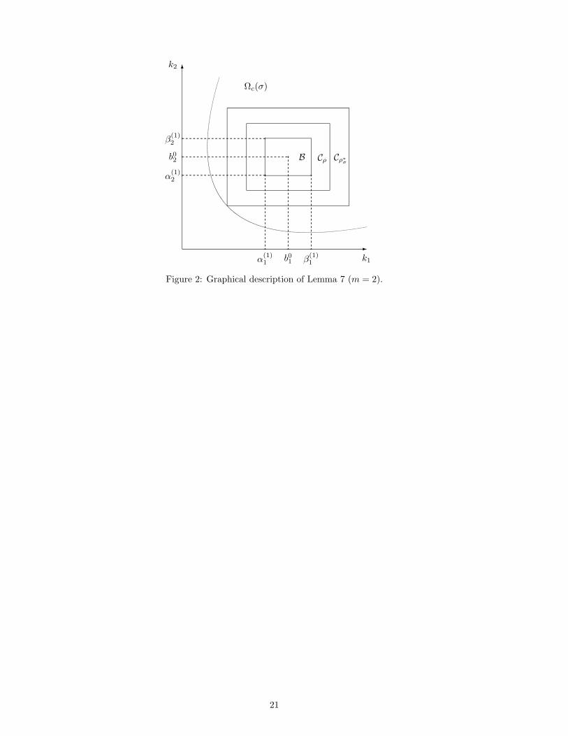
Lemma 7 Let ρ∗σ be the ℓ∞ real parametric stability margin of Pρ with respect to the stability region Sσ, and

consider the one-parameter family of boxes

Cρ :=[

b0 − ρv, b0 + ρv]

, ρ > 0. (23)

Then, the following statements hold

(i) Cρ ⊂ Ωc(σ) ∀ ρ < ρ∗σ

(ii) C1 ≡ B

(iii) Cρ ⊃ B ∀ ρ > 1 .

Proof: By Definition 4 we have that the family of polynomials Pρ has all its roots inside Sσ for any ρ < ρ∗σ.

Consider any ρ such that ρ < ρ∗σ. Then, for any s such that Re[s] ≥ −σ we have

D(s) + b0′N(s) 6= 0 (24)

and

D(s) +m∑

i=1

viNi(s)(

qi + b0i

)

6= 0 , ∀ q : ‖q‖∞ ≤ ρ . (25)

Now, introducing the vector

k = (k1, . . . , km)′ =(

v1(q1 + b01), . . . , vm(qm + b0

m))′

it is easily verified that

‖q‖∞ ≤ ρ ⇔ k ∈ Cρ .

Therefore, exploiting (25), we get that

D(s) + k′N(s) 6= 0 , ∀ s ∈ C\Sσ , ∀ k ∈ Cρ .

From (12), this in turn implies that Cρ ⊂ Ω(σ) for all ρ < ρ∗σ, and by (24) we complete the proof of (i).

The proofs of conditions (ii) and (iii) easily follow from expressions (15) and (23) for B and Cρ, respectively.

10

The above lemma states that the one-parameter family of boxes (23) is such that fulfillment of inequalities

(19) is straightforward (Fig. 2 provides a graphical sketch of the involved sets). Moreover, since Cρ1≤ Cρ2

if

ρ1 ≤ ρ2, exploiting Lemma 6 we arrive at the following final result.

Theorem 8 Let ρ∗σ be the ℓ∞ real parametric stability margin of Pρ with respect to Sσ, and compute

γℓ= sup

σ>0σ − λ∗(σ)

subject to

ρ∗σ > 1 ,

where

λ∗(σ) =1

2T

m∑

i=1

ln

ni∏

j=1

b0i + ρ∗σvi − α

(j)i

b0i + ρ∗σvi − β

(j)i

·β

(j)i − b0

i + ρ∗σvi

α(j)i − b0

i + ρ∗σvi

.

If γℓ> 0, then system ΣL is exponentially stable with a degree of stability at least γ

ℓ.

Remark 4 Since the one-parameter family Cρ in (23) contains only some of the boxes satisfying inequalities

(19), it is clear that γℓ≤ γℓ. However, the computation of γ

ℓis efficiently performed even for large m. Indeed,

for a fixed σ, we simply need to compute the stability margin of the family of polynomials (22) according to

Lemma 2 (see also Remark 2).

5 Application Examples

In this section we consider two examples for illustrating the main features of the lower bounds introduced in

Section 4.

The first example concerns the Brusselator system [Holden & Muhamad, 1986]. All the steps to compute

the lower bound γl

for a given periodic solution are illustrated in detail. In particular, the simplicity of the

computation also in presence of uncertainty on the periodic solution is pointed out. Moreover, the tightness

of the lower bound for slowly varying periodic solutions is enlightened, in agreement with the observation in

Remark 1.

The second example considers a single-mode CO2 laser [Stanghini et al., 1996]. The computation of the

lower bound γl

is performed for a family of periodic solutions generated by a forcing input of increasing

amplitude. In particular, a condition for the existence and an estimation of such a family are provided.

Moreover, the problem of designing a controller able to improve the lower bound γlof the considered family

of periodic solutions is considered at some extent. More details can be found in [Basso et al., 1999] and

[Giovanardi et al., 1999].

5.1 Example 1

As a first application example we consider the following sinusoidally forced version of the Brusselator system

[Holden & Muhamad, 1986]

x1 = a + x21x2 − bx1 − x1 + µ cos( 2π

T t)

x2 = bx1 − x21x2

. (26)

11

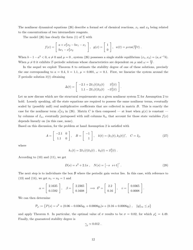
The nonlinear dynamical equations (26) describe a formal set of chemical reactions, x1 and x2 being related

to the concentrations of two intermediate reagents.

The model (26) has clearly the form (1) of Σ with

f(x) =

[

a + x21x2 − bx1 − x1

bx1 − x21x2

]

, g(x) =

[

1

0

]

, w(t) = µ cos( 2πT t) .

When b− 1− a2 < 0, a 6= 0 and µ = 0 , system (26) possesses a single stable equilibrium (x1, x2) = (a, a−1b).

When µ 6= 0 it exhibits T -periodic solutions whose characteristics are dependent on µ and ω = 2πT .

In the sequel we exploit Theorem 8 to estimate the stability degree of one of these solutions, precisely

the one corresponding to a = 0.4, b = 1.1, µ = 0.001, ω = 0.1. First, we linearize the system around the

T -periodic solution x(t) obtaining

∆(t) =

[

−2.1 + 2x1(t)x2(t) x21(t)

1.1 − 2x1(t)x2(t) −x21(t)

]

.

Let us now discuss which are the structural requirements on a given nonlinear system Σ for Assumption 2 to

hold. Loosely speaking, all the state equations are required to possess the same nonlinear terms, eventually

scaled by (possibly null) real multiplicative coefficients that are collected in matrix B. This is exactly the

case for the nonlinear term x21x2 in (26). Matrix C is then composed — at least when g(x) is constant —

by columns of Im, eventually juxtaposed with null columns 0m that account for those state variables f(x)

depends linearly on (in this case, none).

Based on this discussion, for the problem at hand Assumption 2 is satisfied with

A =

[

−2.1 0

1.1 0

]

, B =

[

−1

1

]

, k(t) = (k1(t), k2(t))′, C = I2, (27)

where

k1(t) = 2x1(t)x2(t) , k2(t) = x21(t) .

According to (10) and (11), we get

D(s) = s2 + 2.1s , N(s) =[

−s s+1]′

. (28)

The next step is to individuate the box B where the periodic gain vector lies. In this case, with reference to

(13) and (14), we get n1 = n2 = 1 and

α =

[

2.1635

0.1592

]

, β =

[

2.2365

0.1608

]

=⇒ b0 =

[

2.2

0.16

]

, v =

[

0.0365

0.0008

]

.

We can then determine

Pρ :=

P (s) = s2 + (0.06 − 0.0365q1 + 0.0008q2)s + (0.16 + 0.0008q2) , ‖q‖∞ ≤ ρ

and apply Theorem 8. In particular, the optimal value of σ results to be σ = 0.02, for which ρ∗σ = 4.49.

Finally, the guaranteed stability degree is

γℓ≃ 0.012 .

12

In order to compare such lower bound provided by Theorem 8 with the one obtained via Theorem 4, the

optimization problem of Corollary 5 has been solved for this simple case too, where m = 2. The resulting

bound is

γℓ ≃ 0.017 ,

which is obtained for σ = 0.0235.

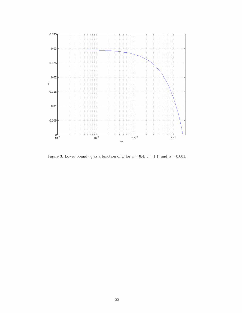
Finally, we briefly investigate the tightness of the lower bound γℓ. As discussed in Remark 1, such a lower

bound is able to recover the actual stability degree γ, when the time variation of the system is arbitrarily

slow. Since in the periodic setting, the time variation is measured by the frequency ω of the forcing term, we

have analyzed the behaviors of γℓ

and γ with respect to ω for a = 0.4 , b = 1.1 and µ = 0.001 . In particular,

we have computed the exact degree of exponential stability for ω = 0, i.e.,

γ(0) = 0.0296 ,

and the lower bound γℓ

for ω ∈ [0.0001, 0.2] . Fig. 3 makes it clear that γℓ(ω) tends to γ(0) for small values

of ω, i.e., the lower bound is tight for slowly varying periodic solutions.

5.2 Example 2

A single-mode CO2 laser can exhibit a cascade of period doubling bifurcations leading to chaos when the cavity

losses are modulated by a sinusoidal signal of increasing amplitude. We consider the control-relevant model

described in [Stanghini et al., 1996], rewritten after a shift of the state variables that moves the equilibrium

of the unforced system into the origin

x = f(x) + Gw − Gu

y = H x ,(29)

where

f(x) =

k0x2

−Γx2 + γRx3 − η[(x2 + 1) exp(x1) − 1]

bx2 − ax3

, G =

k0

0

0

and H = [1 0 0] .

Here, x1 is proportional to the logarithm of the laser intensity, x2 is related to the populations of the two

lasing states, x3 takes also into account the global populations of the manifolds of rotational levels. This laser

system is also provided with a sensed output y ∈ R and a control input u ∈ R, whereas w ∈ R is the forcing

term belonging to the class of signals

W =

wµ(t) = µ cos 2πT t , T = 10−5s , µ ≥ 0 . (30)

The remaining parameters are set as follows

k0 = 3.18 × 107s−1 , γR = 7.0 × 105s−1 ,

Γ = 7.05 × 106s−1 , η = 9.129 × 104s−1 ,

a = 6.767 × 105s−1 , b = 6.626 × 106s−1 .

The objective here is to employ the procedure developed in the preceding section to compute the bounds of

the local exponential stability degrees for the set of T -periodic solutions obtained when the amplitude µ of

13

the forcing term changes. Moreover, we provide some guidelines for the selection of a linear time-invariant

controller which achieves larger stability degrees without a large modification of the original system periodic

solution.

We now state the following proposition to derive a closed-form expression for the T -periodic solution xµ(t)

which is valid for small µ’s. Such an expression will serve us to get the above lower bounds at a very low

computational effort. To this aim, we first need to define the Jacobian of f(x) as the function

J : Rn → Rn×n , J(x) =∂f(x)

∂x.

Proposition 9 Suppose that:

(i) f(0) = 0;

(ii) J(0) has all the eigenvalues in the open left half plane;

(iii) the forcing input w ∈ W.

Then, there exists a positive constant µ such that for all µ ∈ (0, µ) the forced system (29) possesses a unique

non-trivial exponentially stable T -periodic solution5 xµ(t) with the property that

xµ(t) = µ Re

[

(

j2π

TI − J(0)

)−1

G exp

(

j2πt

T

)

]

+ h.o.t. (31)

Since, in the laser system f(0) = 0 and

J(0) =

0 k0 0

−η −Γ−η γR

0 b −a

has all its eigenvalues in the open left half-plane, assumptions (i) and (ii) of Proposition 5 are satisfied, thus

guaranteeing existence of periodic solutions for some interval (0, µ), with the solution given by (31).

The linearization procedure of Section 4 for the whole family of periodic solutions yields the structure of

ΣL given in (9) where

A = J(0) , B =

0

1

0

, kµ(t) =

(

k1(t)

k2(t)

)

= η

(

(x2µ(t) + 1) exp(x1µ(t)) − 1

exp(x1µ(t)) − 1

)

, C =

[

1 0 0

0 1 0

]

.

5The above result simply states that, if the origin of the unforced uncontrolled system is a hyperbolic equilibrium point,

then there exists a family of T -periodic solutions for an interval of the amplitude parameter µ. The proof relies on a suitable

application of the Implicit Function Theorem that exploits the well-known condition for the existence of T -periodic solutions of

finite dimensional linear time invariant systems forced by T -periodic inputs [Khalil, 1992], [Farkas, 1994].

14

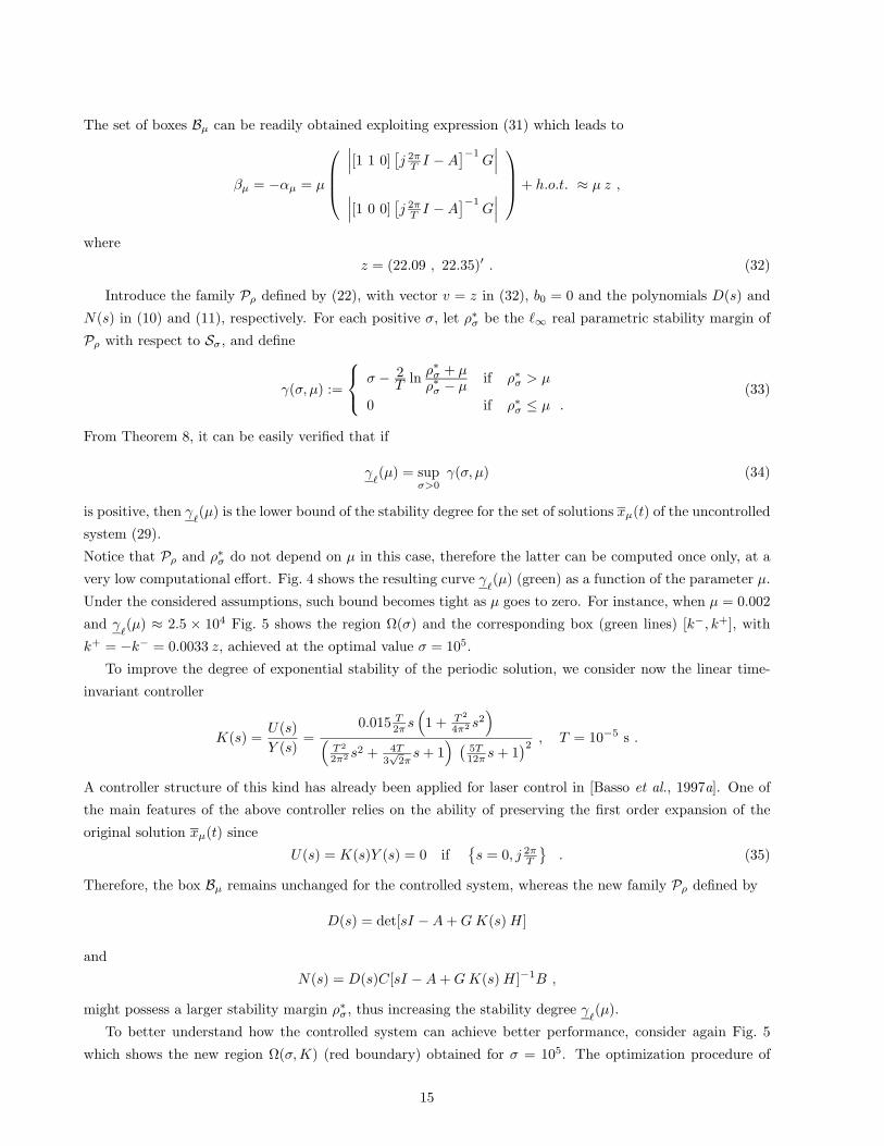
The set of boxes Bµ can be readily obtained exploiting expression (31) which leads to

βµ = −αµ = µ

∣

∣

∣[1 1 0][

j 2πT I − A

]−1G∣

∣

∣

∣

∣

∣[1 0 0][

j 2πT I − A

]−1G∣

∣

∣

+ h.o.t. ≈ µ z ,

where

z = (22.09 , 22.35)′ . (32)

Introduce the family Pρ defined by (22), with vector v = z in (32), b0 = 0 and the polynomials D(s) and

N(s) in (10) and (11), respectively. For each positive σ, let ρ∗σ be the ℓ∞ real parametric stability margin of

Pρ with respect to Sσ, and define

γ(σ, µ) :=

σ − 2T

lnρ∗σ + µρ∗σ − µ

if ρ∗σ > µ

0 if ρ∗σ ≤ µ .(33)

From Theorem 8, it can be easily verified that if

γℓ(µ) = sup

σ>0γ(σ, µ) (34)

is positive, then γℓ(µ) is the lower bound of the stability degree for the set of solutions xµ(t) of the uncontrolled

system (29).

Notice that Pρ and ρ∗σ do not depend on µ in this case, therefore the latter can be computed once only, at a

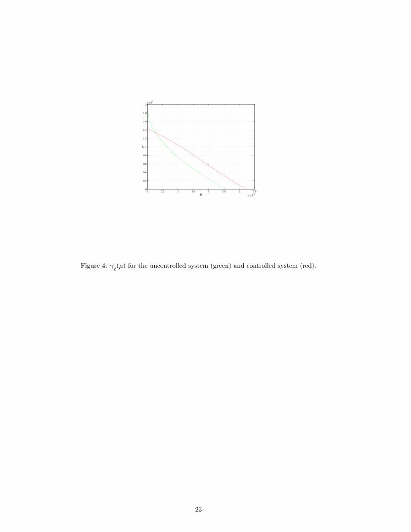
very low computational effort. Fig. 4 shows the resulting curve γℓ(µ) (green) as a function of the parameter µ.

Under the considered assumptions, such bound becomes tight as µ goes to zero. For instance, when µ = 0.002

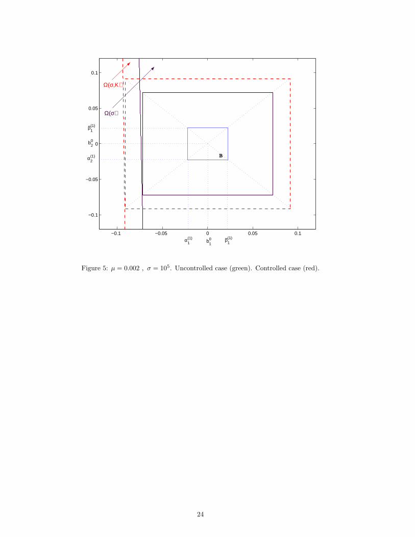
and γℓ(µ) ≈ 2.5 × 104 Fig. 5 shows the region Ω(σ) and the corresponding box (green lines) [k−, k+], with

k+ = −k− = 0.0033 z, achieved at the optimal value σ = 105.

To improve the degree of exponential stability of the periodic solution, we consider now the linear time-

invariant controller

K(s) =U(s)

Y (s)=

0.015 T2π s

(

1 + T 2

4π2 s2)

(

T 2

2π2 s2 + 4T3√

2πs + 1

)

(

5T12π s + 1

)2, T = 10−5 s .

A controller structure of this kind has already been applied for laser control in [Basso et al., 1997a]. One of

the main features of the above controller relies on the ability of preserving the first order expansion of the

original solution xµ(t) since

U(s) = K(s)Y (s) = 0 if

s = 0, j 2πT

. (35)

Therefore, the box Bµ remains unchanged for the controlled system, whereas the new family Pρ defined by

D(s) = det[sI − A + G K(s) H]

and

N(s) = D(s)C[sI − A + G K(s) H]−1B ,

might possess a larger stability margin ρ∗σ, thus increasing the stability degree γℓ(µ).

To better understand how the controlled system can achieve better performance, consider again Fig. 5

which shows the new region Ω(σ,K) (red boundary) obtained for σ = 105. The optimization procedure of

15

Theorem 8 allows us to determine the larger box (red box) [h−, h+] ⊃ [k−, k+], with h+ = −h− = 0.0042 z.

Notice from Fig. 4 (red curve) that the chosen controller K(s) achieves a larger γℓ

not only for the single

solution at µ = 0.002 where γℓ≈ 5.5 × 104, but also for a large interval of the parameter µ.

Obviously, in some cases the above results may be conservative, i.e., xµ(t) will usually have a larger degree

of stability than the one computed via the optimization problem (17). However, the designed controller is

effective in improving the stability degree not only for the specified solution xµ(t), but for a whole class of

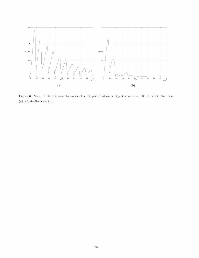
solutions. For example, Figs. 6(a)-(b) show the improvement in the norm of the transient behavior of a 1%

perturbation on xµ(t) when µ = 0.03, for the uncontrolled and controlled case, respectively.

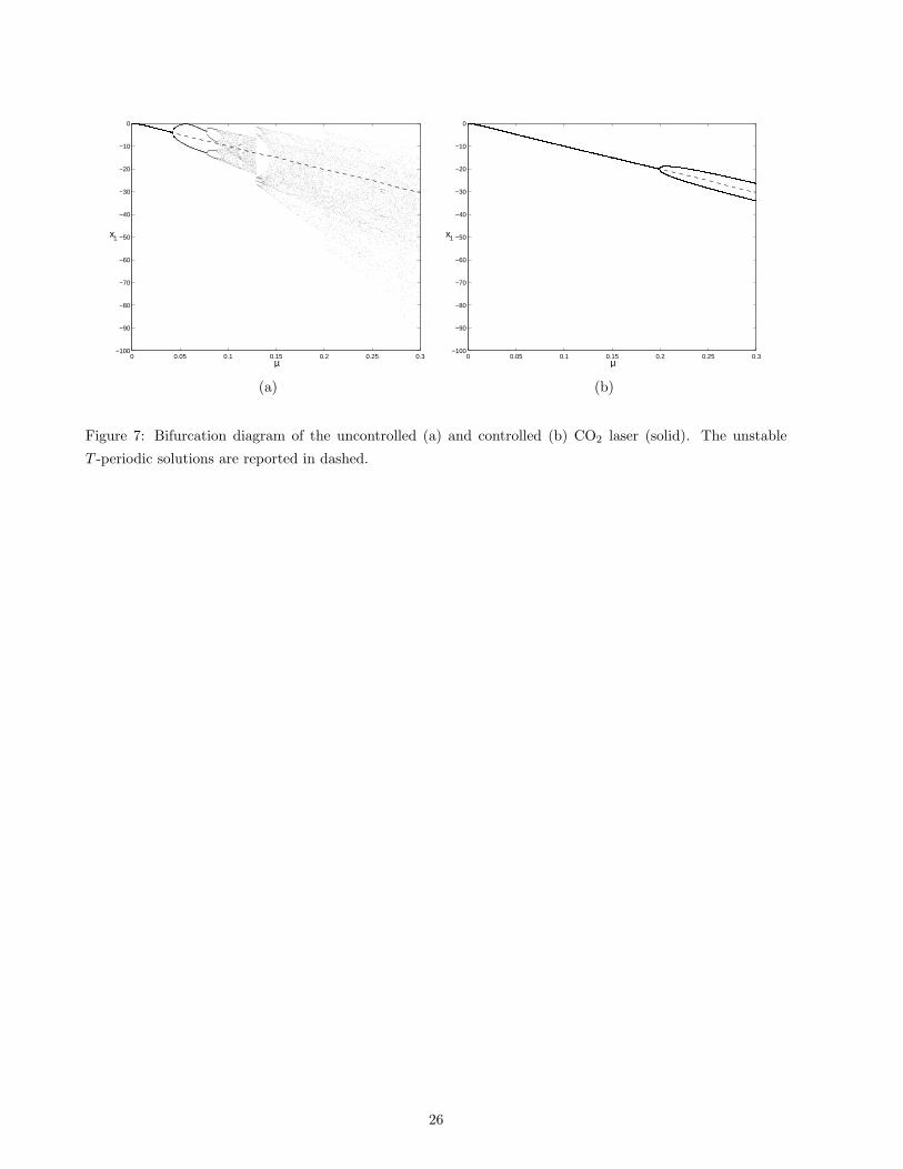
Moreover, an interesting side-effect of improving the stability degree of a periodic solution relies in the

ability of shifting a possible bifurcation, which is the critical parameter µ∗ where the solution xµ∗(t) looses

its stability, to larger values of µ. This is evident when comparing the bifurcation diagrams of Fig. 7(a)

(uncontrolled case) and Fig. 7(b) (controlled case). Indeed, the controller K(s) succeeds in shifting the

bifurcation from µ∗0 ≃ 0.042 to µ∗ ≃ 0.2, and at the same time it does not modify significantly the shape of

the T -periodic solutions, as required in the control design problem. Consequently, the chaotic behavior which

occurs in the uncontrolled system when µ > 0.09 is totally suppressed (see Figs. 7(a)-(b)).

6 Conclusions

The paper has considered the problem of estimating the degree of local exponential stability of periodic

solutions in a class of forced nonlinear systems. Some estimations of the degree of stability are provided by

mixing results concerning the stability of linear time varying systems and the robust stability of uncertain

linear time invariant systems. In particular, a well-known integral-logarithmic criterion for the stability of

linear time varying systems is tailored to our periodic setting and the real parametric stability margin of a

family of polynomials is used to obtain a lower bound of the degree of stability. Although it is in general

conservative with respect the actual degree of stability obtainable via the Floquet-based approach, such a lower

bound possesses interesting features. It can be easily computed also if the periodic solution is not exactly

known. Moreover, it can be used as an efficient measure for the design of controllers ensuring a satisfactory

transient behavior of the considered periodic solutions. Two application examples are discussed in detail for

illustrating the above features.

References

Abed, E. H. & Wang, H. O. [1995] “Feedback control of bifurcations and chaos in dynamical systems,”

in Recent Developments in Stochastic and Nonlinear Dynamics: Applications to Mechanical Systems,

eds. Namachchivaya, N. S. & Kliemann, W. (CRC Press, Boca Raton, FL).

Basso, M., Genesio, R., Giovanardi, L. & Tesi, A. [1998] “On optimal stabilization of periodic orbits via

time-delayed feedback control,” Int. J. Bifurcation and Chaos 8, 1699–1706.

Basso, M., Genesio, R. & Tesi, A. [1997a] “Controller design for extending periodic dynamics of a chaotic co2

laser,” Systems and Control Letters 31, 287–297.

Basso, M., Genesio, R. & Tesi, A. [1997b] “Stabilizing periodic orbits of forced systems via generalized pyragas

controllers,” IEEE Trans. Circ. and Syst. - I 44, 1023–1027.

16

Basso, M., Giovanardi, L., Genesio, R. & Tesi, A. [1999] “An approach for stabilizing periodic orbits in

nonlinear systems,” in Proc. of the 5th European Control Conference (Karlsruhe).

Bhattacharyya, S., Chapellat, H. & Keel, L. [1995] Robust Control: The Parametric Approach (Prentice Hall

PTR, Upper Saddle River, NJ).

Dasgupta, S., Chockalingam, G., Anderson, B. & Fu, M. [1994] “Lyapunov functions for uncertain systems

with application to the stability of time varying systems,” IEEE Trans. Circ. and Syst. - I 41, 93–106.

(eds.) Chen, G. [1999] in Controlling Chaos and Bifurcations in Engineering Systems (CRC Press, Boca Raton,

FL).

(eds.) Garulli, A., Tesi, A. & Vicino, A. [1999] “Robustness in identification and control,” in Lecture notes in

Control and Information Sciences Vol. 245 (Springer-Verlag, London).

Farkas, M. [1994] Periodic Motion (Springer-Verlag, New York).

Freedman, M. & Zames, G. [1968] “Logarithmic variation criteria for the stability of systems with time varying

gains,” SIAM J. Control 6(3), 487–507.

Giovanardi, L., Basso, M., Genesio, R. & Tesi, A. [1999] “Controller design for improving the degree of stability

of periodic solutions in forced nonlinear systems,” in Proc. of the 38th IEEE Conference on Decision and

Control (Phoenix).

Holden, A. & Muhamad, M. [1986] “A graphical zoo of strange and peculiar attractors,” in Chaos, ed. Holden,

A. (University Press, Manchester).

Just, W., Bernard, T., Ostheirer, M., Reibold, E. & Benner, H. [1997] “Mechanism of time-delayed feedback

control,” Phys. Rev.Lett. 78, 203–206.

Khalil, H. K. [1992] Nonlinear Systems, 2nd edn (Macmillan, New York).

Nayfeh, A. H. & Balachandran, B. [1995] Applied Nonlinear Dynamics (Wiley, New York).

Ott, E., Grebogi, C. & Yorke, J. A. [1990] “Controlling chaos,” Phys. Rev. Lett. 64, 1196–1199.

Pyragas, K. [1992] “Continuous control of chaos by self-controlling feedback,” Phys..Lett. A 170, 421–428.

Romeiras, F. J., Grebogi, C., Ott, E. & Dayawansa, W. P. [1992] “Controlling chaotic dynamical systems,”

Physica D 58, 165–192.

Socolar, J. E. S., Sukow, D. W. & Gauthier, D. J. [1994] “Stabilizing unstable periodic orbits in fast dynamical

systems,” Phys. Rev. E 50, 3245–3248.

Stanghini, M., Basso, M., Genesio, R., Tesi, A., Meucci, R. & Ciofini, M. [1996] “A new three-equation model

for the co2 laser,” IEEE J. Quantum Electronics 32, 1126–1131.

Vidyasagar, M. [1993] Nonlinear System Analysis, 2nd edn (Prentice-Hall, Englewood Cliffs, NJ).

17

Appendix

Proof of Lemma 2

Several proofs of the result given in Lemma 2 are available in the literature (for instance, see [Bhattacharyya

et al., 1995, Chapter 4]). For completeness of the paper, a proof tuned on the adopted notation is reported

below.

From Definition 4, the ℓ∞ real parametric stability margin can be written as

ρ∗σ = infω≥0

rσ(ω) (36)

where

rσ(ω) = minq

‖q‖∞

subject to (37)

1 − q′G(σ + jω) = 0 .

Therefore, for each ω ≥ 0, we have to compute rσ(ω).

First, suppose that ω ∈ Π(I)σ . Then, (37) reduces to

rσ(ω) = minq

‖q‖∞

subject to (38)

1 − q′Rσ(ω) = 0

and thus we obtain

rσ(ω) =1

‖Rσ(ω)‖1

. (39)

Now, suppose that ω ∈ Π(II)σ . Then, (37) can be equivalently written as

rσ(ω) = minq

‖q‖∞

subject to[

R′σ(ω)

I ′σ(ω)

]

q =

[

1

0

]

.

Exploiting a standard result of duality theory, we have

rσ(ω) = maxλ1,λ2∈R

λ1

subject tonq∑

i=1

|λ1rσi(ω) + λ2iσi

(ω)| ≤ 1 .

It is easily checked that rσ(ω) has the following expression

rσ(ω) = maxi=1,...,nq

|iσi(ω)|

∑nq

j=1

∣

∣rσj(ω)iσi

(ω) − iσj(ω)rσi

(ω)∣

∣

. (40)

Therefore, Eqs. (36), (39) and (40) complete the proof.

18

Proof of Theorem 4

Conditions (i) of Theorem 4 and Lemma 1 are equivalent since the analysis can be restricted to the finite

interval [0, T ] and k(t) ∈ B on the same interval. According to (10)–(12) and (5), the equivalence between

condition (ii) of Theorem 4 and Lemma 1 easily follows from the relation

det[sI − A − Bk′C] = D(s) + k′N(s) .

Parameter T in condition (iii) can be here chosen equal to the period of the oscillation. With this choice the

integral is independent of t, so that maximization over all t ≥ 0 is not needed anymore. Thus, we can set

t = 0 and integrate over the fixed interval [0, T ].

Now, for each 1 = 1, . . . ,m, define the non-decreasing continuous functions

hi : (k−i , k+

i ) 7−→ R , x −→ lnx − k−

i

k+i − x

.

Since hi[ki(t)] is T -periodic,

0 =

∫ T

0

d

dτhi[ki(τ)] dτ =

∫ T

0

[

d

dτhi[ki(τ)]

]+

dτ +

∫ T

0

[

d

dτhi[ki(τ)]

]−

dτ ,

so that

∫ T

0

∣

∣

∣

∣

d

dτhi[ki(τ)]

∣

∣

∣

∣

dτ =

∫ T

0

[

d

dτhi[ki(τ)]

]+

dτ −

∫ T

0

[

d

dτhi[ki(τ)]

]−

dτ = 2 ·

∫ T

0

[

d

dτhi[ki(τ)]

]+

dτ .

Exchanging the order of summation and integration operators and summing over i proves equivalence of

relations (3) and (4) in the periodic case.

Last step is to derive condition (16): using monotonicity of hi(·), we have

m∑

i=1

∫ T

0

[

d

dτhi[ki(τ)]

]+

dτ =m∑

i=1

ni∑

j=1

[

hi(β(j)i ) − hi(α

(j)i )]

=m∑

i=1

ln

ni∏

j=1

β(j)i − k−

i

k+i − β

(j)i

·k+

i − α(j)i

α(j)i − k−

i

.

19

B

k1

k2

k−1 k+

1α(1)1

b01 β

(1)1

k−2

k+2

α(1)2

b02

β(1)2

Ωc(σ)

Figure 1: Quantities involved in application of Theorem 4 for m = 2.

20

k1

k2

α(1)1

b01 β

(1)1

α(1)2

b02

β(1)2

Ωc(σ)

Cρ∗

σCρB

Figure 2: Graphical description of Lemma 7 (m = 2).

21

10−4

10−3

10−2

10−1

0

0.005

0.01

0.015

0.02

0.025

0.03

0.035

ω

γ

Figure 3: Lower bound γℓ

as a function of ω for a = 0.4, b = 1.1, and µ = 0.001.

22

0 0.5 1 1.5 2 2.5 3 3.5

x 10−3

0

0.2

0.4

0.6

0.8

1

1.2

1.4

1.6

1.8

2x 10

5

µ

γl

Figure 4: γℓ(µ) for the uncontrolled system (green) and controlled system (red).

23

−0.1 −0.05 0 0.05 0.1

−0.1

−0.05

0

0.05

0.1

Ω(σ,Κ)

b01

b02

α1(1) β

1(1)

α2(1)

β1(1)

B

Ω(σ)

Figure 5: µ = 0.002 , σ = 105. Uncontrolled case (green). Controlled case (red).

24

0 0.1 0.2 0.3 0.4 0.5 0.6 0.7 0.8 0.9 1

x 10−4

0

0.5

1

1.5

Time

||δ xµ(t)||

0 0.1 0.2 0.3 0.4 0.5 0.6 0.7 0.8 0.9 1

x 10−4

0

0.5

1

1.5

Time

||δ xµ(t)||

(a) (b)

Figure 6: Norm of the transient behavior of a 1% perturbation on xµ(t) when µ = 0.03. Uncontrolled case

(a). Controlled case (b).

25

0 0.05 0.1 0.15 0.2 0.25 0.3−100

−90

−80

−70

−60

−50

−40

−30

−20

−10

0

µ

x1

0 0.05 0.1 0.15 0.2 0.25 0.3−100

−90

−80

−70

−60

−50

−40

−30

−20

−10

0

µ

x1

(a) (b)

Figure 7: Bifurcation diagram of the uncontrolled (a) and controlled (b) CO2 laser (solid). The unstable

T -periodic solutions are reported in dashed.

26