Lower Bound for Sorting Complexity

Lecture 9 COMPSCI 220 - AP G. Gimel'farb 1

Lower Bound for Sorting Complexity

• Theorem 2.30: Any algorithm that sorts by comparing onlypairs of elements must use at least

log2(n!) ≅ n log2 n − 1.44n comparisons in the worst case (that is, for some “worst”

input sequence) and in the average case– Stirling's approximation of the factorial (n!):

!

1 " 2 " ... " n # n! $ ne( )

n

2%n & 2.5nn+ 0.5

e'n


Decision Tree for Sorting n Items

Decision tree for n =3:• i:j - a comparison of

ai and aj

• ijk - a sorted array(ai aj ak)

• n! permutations ⇒ n! leaves

Sorting in descending order of the numbers


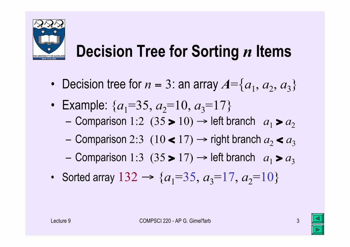
Decision Tree for Sorting n Items

• Decision tree for n = 3: an array A={a1, a2, a3}• Example: {a1=35, a2=10, a3=17}

– Comparison 1:2 (35 > 10) → left branch a1 > a2

– Comparison 2:3 (10 < 17) → right branch a2 < a3

– Comparison 1:3 (35 > 17) → left branch a1 > a3

• Sorted array 132 → {a1=35, a3=17, a2=10}


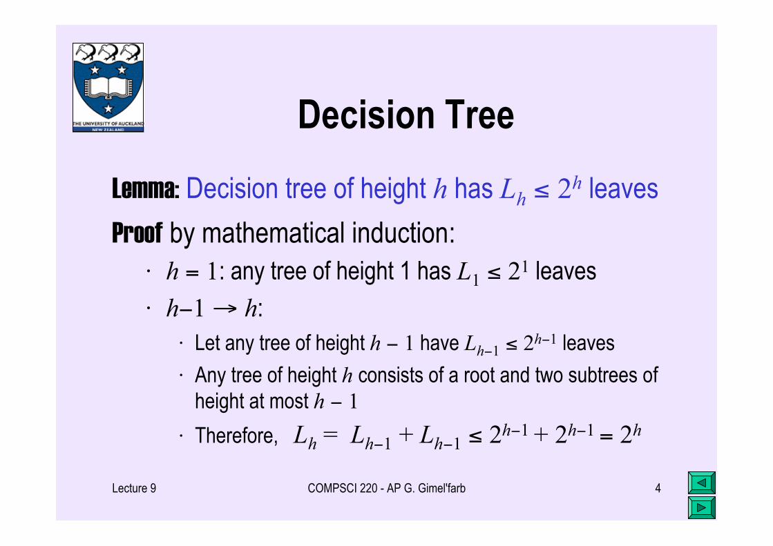
Decision Tree

Lemma: Decision tree of height h has Lh ≤ 2h leaves

Proof by mathematical induction:· h = 1: any tree of height 1 has L1 ≤ 21 leaves

· h−1 → h:· Let any tree of height h − 1 have Lh−1 ≤ 2h−1 leaves

· Any tree of height h consists of a root and two subtrees ofheight at most h − 1

· Therefore, Lh = Lh−1 + Lh−1 ≤ 2h−1 + 2h−1 = 2h


Worst-Case Complexity of Sorting

• Theorem 2.32: The worst-case complexity of sortingn items by pairwise comparisons is Ω(n log n)

• Proof:– Any decision tree of height h has at most 2h leaves (see

Lemma, Slide 4)

– The least height h such that Lh = 2h ≥ n! leaves is

h ≥ log2( n!) ≅ n log2 n − 1.44 n


Bucket Sort (Exercise 2.6.2)

Let all integers to sort in an array a of size n be in thefixed range [1,…,qmax]

1. Introduce a counter array t of size qmax and set itsentries initially to zero

2. Scan through a to accumulate in the counters t[i];i = 0,…,qmax−1, how many times each item i + 1is found in a

3. Loop through 0 ≤ i ≤ qmax−1 and output t[i]copies of integer i + 1 at each step


Bucket Sort (Exercise 2.6.2)

Worst- and average-case time complexity of bucketsort is Θ(n) provided that qmax is fixed

– qmax + n elementary operations to first set t tozero and then count how many times t[i] eachitem i + 1 is found in a

– qmax + n elementary operations to successivelyoutput the sorted array a by repeating t[i] timeseach entry i + 1

Theorem 2.30 does not hold under additional constraints!


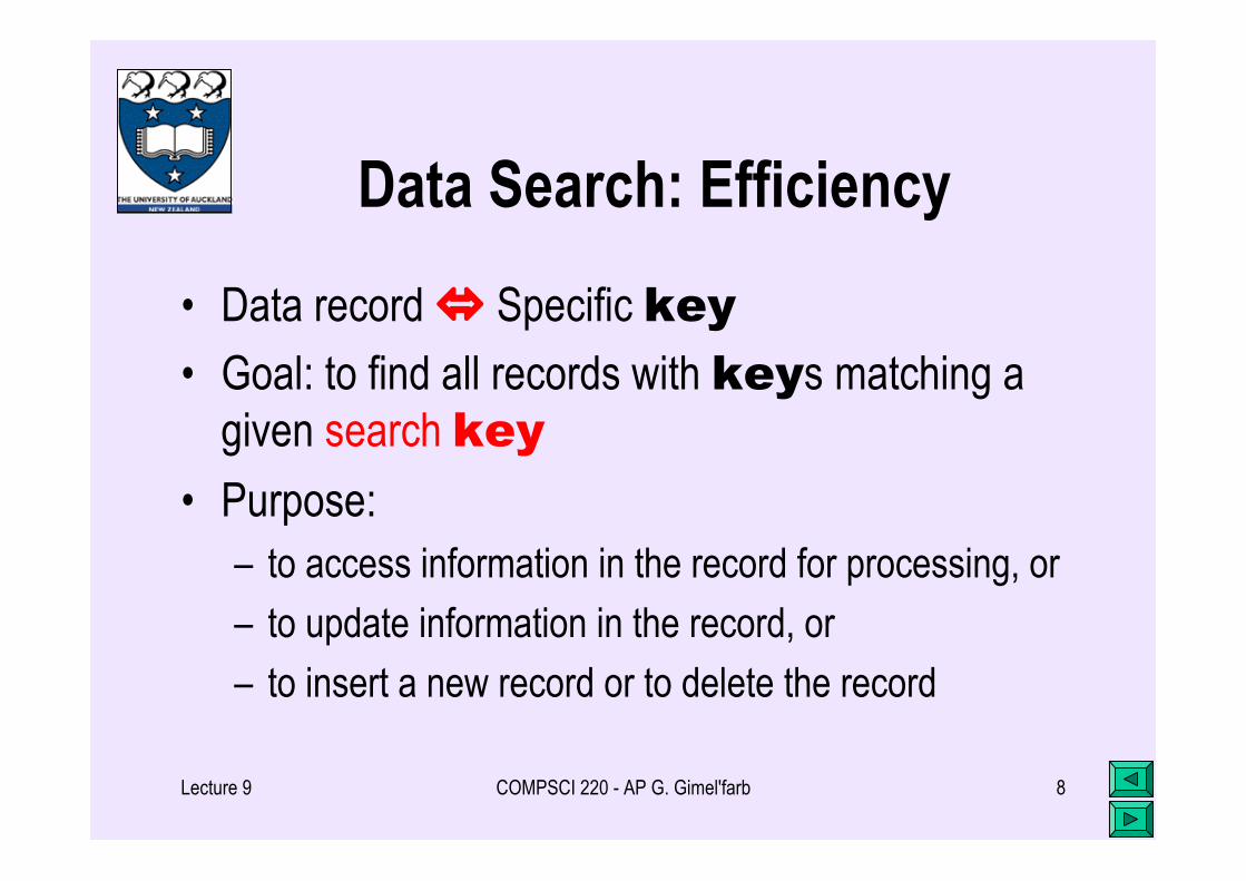
Data Search: Efficiency

• Data record Specific key

• Goal: to find all records with keys matching agiven search key

• Purpose:– to access information in the record for processing, or

– to update information in the record, or

– to insert a new record or to delete the record


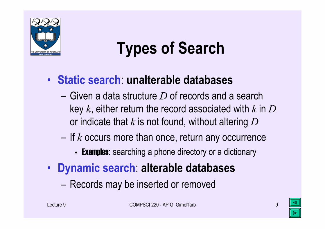
Types of Search

• Static search: unalterable databases– Given a data structure D of records and a search

key k, either return the record associated with k in Dor indicate that k is not found, without altering D

– If k occurs more than once, return any occurrence• Examples: searching a phone directory or a dictionary

• Dynamic search: alterable databases– Records may be inserted or removed


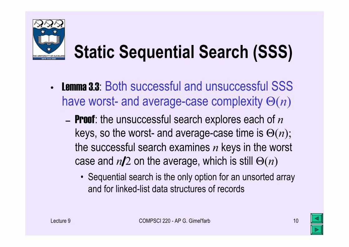
Static Sequential Search (SSS)

• Lemma 3.3: Both successful and unsuccessful SSShave worst- and average-case complexity Θ(n)– Proof: the unsuccessful search explores each of n

keys, so the worst- and average-case time is Θ(n);the successful search examines n keys in the worstcase and n/2 on the average, which is still Θ(n)

• Sequential search is the only option for an unsorted arrayand for linked-list data structures of records


Static Binary Search O(log n)

• Ordered array: key0 < key1 < … < keyn−1

• Compare the search key with the record keyi atthe middle position i = (n−1)/2– if key = keyi, return i– if key < keyi or key < keyi, then it must be in

the 1st or in the 2nd half of the array, respectively

• Apply the previous two steps to the chosen half of thearray iteratively (repeating halving principle)


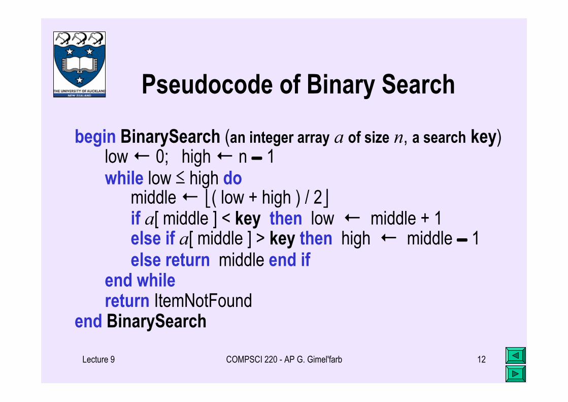
Pseudocode of Binary Search

begin BinarySearch (an integer array a of size n, a search key) low ← 0; high ← n − 1 while low ≤ high do middle ← ( low + high ) / 2 if a[ middle ] < key then low ← middle + 1 else if a[ middle ] > key then high ← middle − 1 else return middle end if end while return ItemNotFoundend BinarySearch


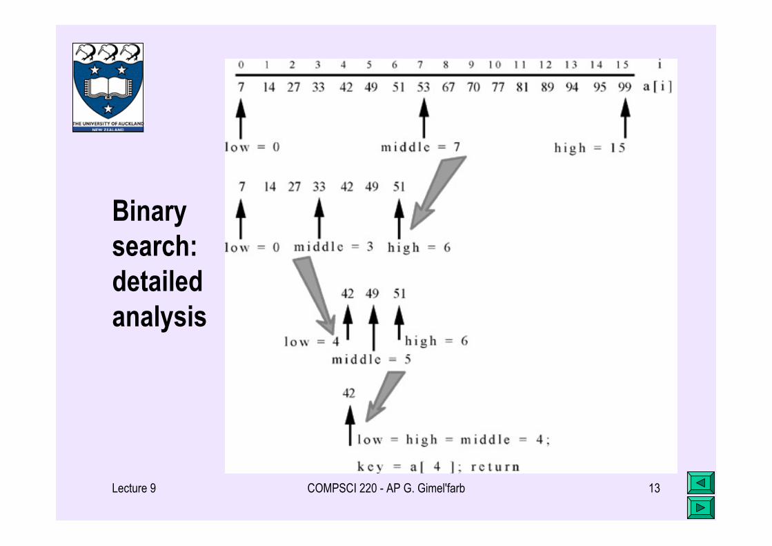
Binarysearch:detailedanalysis


Comparisonstructure:the binary

(search) tree


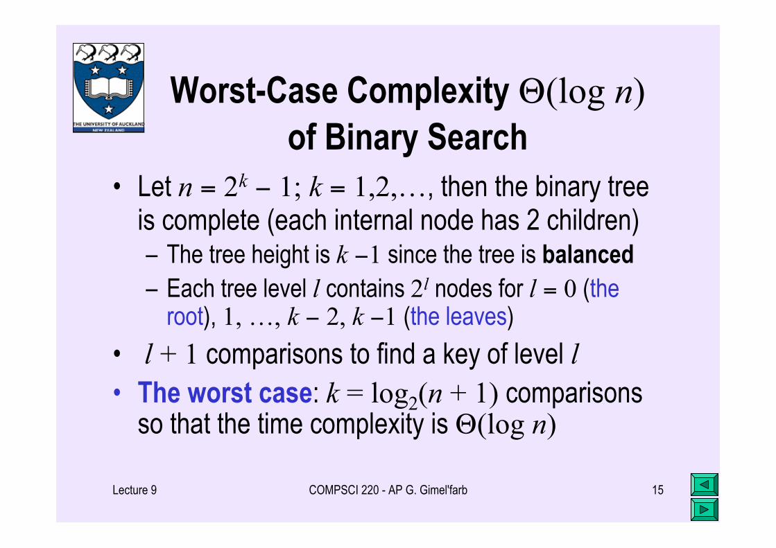
Worst-Case Complexity Θ(log n)of Binary Search

• Let n = 2k − 1; k = 1,2,…, then the binary treeis complete (each internal node has 2 children)– The tree height is k −1 since the tree is balanced– Each tree level l contains 2l nodes for l = 0 (the

root), 1, …, k − 2, k −1 (the leaves)

• l + 1 comparisons to find a key of level l• The worst case: k = log2(n + 1) comparisons

so that the time complexity is Θ(log n)


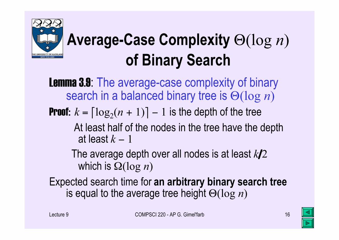
Average-Case Complexity Θ(log n)of Binary Search

Lemma 3.9: The average-case complexity of binarysearch in a balanced binary tree is Θ(log n)

Proof: k = log2(n + 1) − 1 is the depth of the tree At least half of the nodes in the tree have the depth

at least k − 1 The average depth over all nodes is at least k/2

which is Ω(log n)Expected search time for an arbitrary binary search tree

is equal to the average tree height Θ(log n)


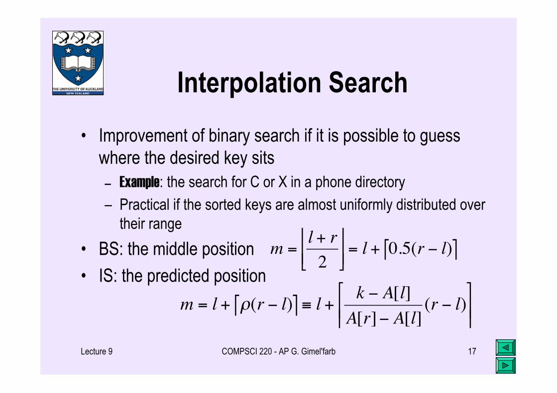
Interpolation Search

• Improvement of binary search if it is possible to guesswhere the desired key sits

– Example: the search for C or X in a phone directory

– Practical if the sorted keys are almost uniformly distributed overtheir range

• BS: the middle position

• IS: the predicted position

!

m =l + r

2

"

# " $

% $ = l + 0.5(r & l)' (

!

m = l + "(r # l)$ % & l +k # A[l]

A[r]# A[l](r # l)

$

' '

%

( (


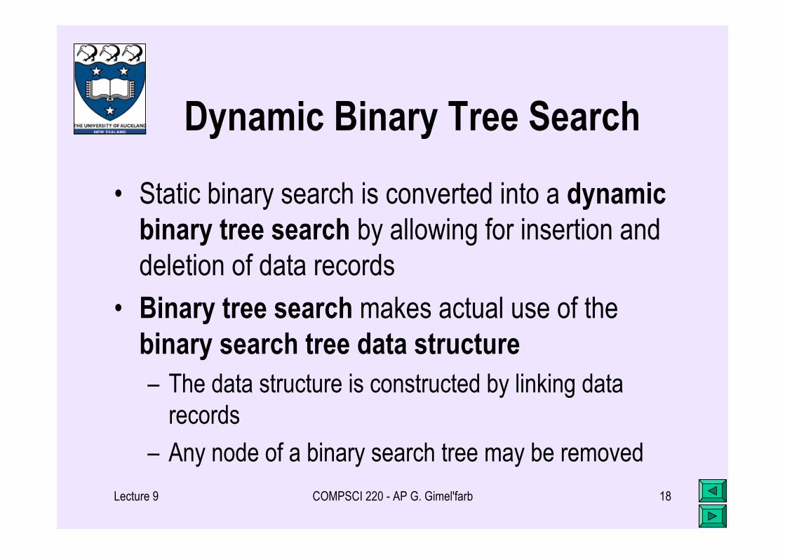
Dynamic Binary Tree Search

• Static binary search is converted into a dynamicbinary tree search by allowing for insertion anddeletion of data records

• Binary tree search makes actual use of thebinary search tree data structure– The data structure is constructed by linking data

records

– Any node of a binary search tree may be removed

Lower Bound for Sorting Complexity

Documents