Low-ozone bubbles observed in the tropical tropopause layer during the TC4 campaign in 2007

Low‐ozone bubbles observed in the tropical tropopauselayer during the TC4 campaign in 2007

I. Petropavlovskikh,1,2 E. Ray,1,2 S. M. Davis,1,2 K. Rosenlof,2 G. Manney,3,4 R. Shetter,5

S. R. Hall,5 K. Ullmann,5 L. Pfister,6 J. Hair,7 M. Fenn,8 M. Avery,7

and A. M. Thompson9

Received 9 July 2009; revised 15 April 2010; accepted 22 April 2010; published 10 September 2010.

[1] In the summer of 2007, the NASA DC‐8 aircraft took part in the TropicalComposition, Cloud and Climate Coupling campaign based in San Jose, Costa Rica.During this campaign, multiple in situ and remote‐sensing instruments aboard the aircraftmeasured the atmospheric composition of the tropical tropopause layer (TTL) in theequatorial region around Central and South America. During the 17 July flight off theEcuadorian coast, well‐defined “bubbles” of anomalously low‐ozone concentration (lessthan 75 ppbv) were detected above the aircraft in the TTL at the altitude near 365 K(between 14 and 16 km) and at ∼3°S and ∼82°W. Backward trajectories frommeteorological analyses and the aircraft in situ measurements suggest that the ozone‐depleted air mass originated from deep convection in the equatorial eastern Pacific and/orPanama Bight regions at least 5 days before observation by the DC‐8; this was not afeature produced by local convection. Given uncertainties known in regard to trajectoriescalculated from global reanalysis, it is not possible to identify the exact convective systemthat produced this particular low‐ozone anomaly, but only the general origin from aregion of high convective activity. However, the fact that the feature apparentlymaintained its coherency for at least 5 days suggests a significant contribution to thechemical composition of the tropical upper troposphere portion of the TTL fromconvective systems followed by quasi‐horizontal transport. It also suggests that mixingtime scales for these relatively small spatial features are greater than 5 days.

Citation: Petropavlovskikh, I., et al. (2010), Low‐ozone bubbles observed in the tropical tropopause layer during the TC4campaign in 2007, J. Geophys. Res., 115, D00J16, doi:10.1029/2009JD012804.

1. Introduction

[2] Ozone changes in the tropical lower stratosphere areimportant for determining the magnitude and sign of theozone radiative forcing [IPCC, 2001]. Additionally, asnoted by Gettelman et al. [2009], modeled tropopauseheight levels and cold point temperatures are sensitive to theamount of ozone near the tropopause. The photochemical

lifetime of ozone in the tropical tropopause layer (TTL) withrespect to the chemical production and loss is severalmonths, so transport is the primary cause of changes inozone mixing ratios [Folkins et al., 2002; Fueglistaler et al.,2009; Rivière et al., 2006; Wennberg et al., 1998]. Becausethe TTL serves as the gateway for air entering the strato-sphere, it is of interest to study processes that impact thedistribution of radiatively and chemically important gases inthat region. In this study, we examine a specific case inwhich low‐ozone air from low altitudes is transported intothe tropical upper troposphere and maintains its integrity fora number of days, demonstrating the importance of con-vective transport to establishing species concentrations inthe tropical upper troposphere.[3] In the summer of 2007, the NASA DC‐8 aircraft took

part in the Tropical Composition, Cloud and Climate Cou-pling (TC4) campaign based in Costa Rica [Pfister et al.,2010; Toon et al., 2010]. Multiple in situ and remote‐sensing instruments aboard the aircraft were flown to mea-sure atmospheric composition of the TTL. The layer wasfirst defined by Highwood and Hoskins [1998] and Folkinset al. [1999] as the transitional layer in the tropics (located at∼12–18 km altitude) that is significantly impacted by deep

1Cooperative Institute for Research in Environmental Sciences,University of Colorado, Boulder, Colorado, USA.

2Earth Systems Research Laboratory, NOAA, Boulder, Colorado, USA.3Jet Propulsion Laboratory, California Institute of Technology,

Pasadena, California, USA.4New Mexico Institute of Mining and Technology, Socorro, New

Mexico, USA.5National Center for Atmospheric Research, ESSL, Atmospheric

Chemistry Division, Boulder, Colorado, USA.6NASA Ames Research Center, Moffett Field, California, USA.7NASA Langley Research Center, Hampton, Virginia, USA.8Science Systems and Applications, Inc., Hampton, Virginia, USA.9Meteorology Department, Pennsylvania State University, University

Park, Pennsylvania, USA.

Copyright 2010 by the American Geophysical Union.0148‐0227/10/2009JD012804

JOURNAL OF GEOPHYSICAL RESEARCH, VOL. 115, D00J16, doi:10.1029/2009JD012804, 2010

D00J16 1 of 15

http://dx.doi.org/10.1029/2009JD012804

convection, and the chemical composition of which istransitional between the “convectively dominated tropicaltroposphere and the radiatively controlled stratosphere”[Gettelman and Forster, 2002]. Fueglistaler et al. [2009]defined the layer slightly differently, extending it furtherinto the tropical stratosphere.[4] In this study, observations are described only in the

tropospheric portion of the TTL, from ∼150 hPa or 15 km tothe tropopause. On the 17 July 2007 TC4 flight of theNASA DC‐8, a bubble of depleted ozone between 14 and16 km was observed near the coast of Ecuador by severalinstruments. A similar ozone feature is found in a satelliteozone profile and is also consistent with satellite measuredtotal ozone column data on that day. Analyses of an ozonesounding data climatology over several Intertropical Con-vergence Zone (ITCZ) ground stations often show the typ-ical S‐shaped vertical structure near 15 km that is indicativeof the ongoing convective process [Thompson et al., 2010].This indicates that such phenomena are not an uncommonoccurrence and hence likely contribute to the overall ozonebudget in the UT. Convective signatures are not necessarilylocal and recent; however, advection and wave activity alsoplay a role in ozone structure near the TTL [Selkirk et al.,2010; Thompson et al., 2010]. Thus, it is of interest tostudy this particular case observed by the DC‐8 to focus onquestions concerning the impact of convection and timescales for chemistry and transport affecting the compositionof the TTL [Fueglistaler et al., 2009]. Sections 2 and 3describe ground and aircraft data associated with theobserved low‐ozone event. Section 4 describes the backtrajectory analysis of the low‐ozone parcel transport beforethe observation. Section 5 presents satellite data for confir-mation of the spatial and temporal extend of the low‐ozone

parcel. Further exploration of the long‐range isentropicozone transport hypothesis is done in section 6 by usingreverse domain filling (RDF) calculations driven by assim-ilated meteorological analyses and initialized with satelliteozone. Section 7 summarizes TC4 results discussed in otherTC4 special issue papers that are relevant to the TTLcomposition affected by local convection processes, waveactivity, pollution from the boundary layer, and long‐termozone climatology. Section 8 concludes that local convec-tion can be excluded as a possible explanation for the low‐ozone bubbles observed in the TTL by the TC4 aircraftinstruments.

2. Measurements and Data

[5] The TC4 campaign was based out of San Jose, CostaRica, during July and August 2007. Measurements werecoordinated between three aircraft, providing coverage ofthe stratosphere (ER‐2), upper troposphere (WB‐57), andlow to middle troposphere (DC‐8). In this study, weexclusively use measurements from the DC‐8, as the flightof interest did not have simultaneous measurements fromthe other two aircraft. The DC‐8 aircraft was equipped withboth in situ and remote‐sensing instruments. Measurementsof ozone, aerosol, cloud, water vapor, and other trace gasseswere taken from aboard the aircraft. A key measurement forthis study was from the DC‐8‐borne CCD‐based ActinicFlux Spectroradiometer (CAFS) [Petropavlovskikh et al.,2007], which has been used in previous satellite validationcampaigns [Kroon et al., 2008; Petropavlovskikh et al.,2008]. Other relevant DC‐8 measurements included nadirand zenith ozone, aerosol, and depolarization profiles fromthe differential absorption lidar (DIAL) system [Browell,

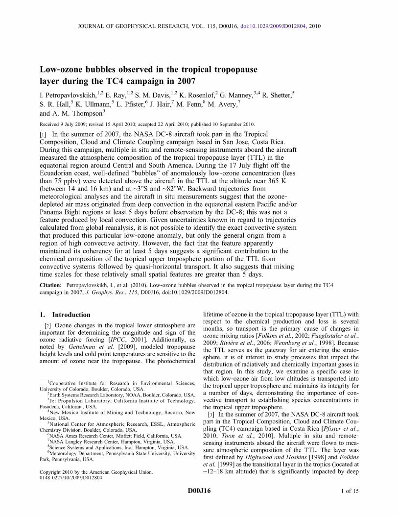
Figure 1. NASA DC‐8 aircraft tracks (gray scale indicates altitude of the aircraft, and blue numbersindicate time in UT) and DOAS‐OMI total ozone swath on 17 July 2007 during the TC4 campaign inJuly–August 2007 (courtesy of the OMI team).

PETROPAVLOVSKIKH ET AL.: OZONE BUBBLES IN TROPICAL TROPOPAUSE LAYER D00J16D00J16

2 of 15

1981; 1989; Browell et al., 1998]; in situ ozone mixingratios from the FastOz system [Avery et al., 2010; Pearsonand Stedman, 1980] using the fast‐response nitric oxidechemiluminesence method; carbon monoxide (CO) mea-surements from the differential absorption CO measurementinstrument [Sachse et al., 1987]; and tropical ozonesondeslaunched from Las Tablas, Panama (7.8°N, 80°W) [Thompsonet al., 2010, G. Morris et al., Observations of ozone productionin a dissipating tropical convective cell during TC‐4, sub-mitted to Atmospheric Chemistry and Physics Discussion,2010], Juan Santa Maria airport, Costa Rica (10°N, 84°W)[Selkirk et al., 2010], San Cristobal, Galapagos Islands (1°S,90°W), and Paramaribo, Ecuador (5.8°N, 55°W). The CostaRica, San Cristobal, and Paramaribo sites are part of theSouthern Hemisphere Additional Ozonesondes network. Inaddition to the daily ozonesondes at Panama, continuoussurface ozone measurements from the Nittany AtmosphericTrailer and Integrated Validation Experiment were alsotaken. Measurements from all of these instruments have beenused in past satellite validation campaigns [Froidevaux andDouglass, 2001; Newman et al., 2001] and for scientificprocess studies.[6] The DC‐8 sampled the atmosphere over a very large

region near equatorial Central and South America [Toonet al., 2010]. However, the phenomenon we discuss in thisstudy, a low ozone bubble near the coast of Ecuador, was theonly one observed by the DC‐8 during the TC4 mission.Figure 1 shows the NASA DC‐8 flight tracks on 17 July2007 plotted over the map of coincident Aura OzoneMonitoring Instrument (OMI) total ozone data (orbit 15982)[Levelt et al., 2006a, 2006b]. There are two ozone productsthat are available from the OMI ultraviolet‐visible images ofthe Earth [Kroon et al., 2008; McPeters et al., 2008]. One

method (OMI‐Total Ozone Mapping Spectrometer (TOMS))is based on the traditional TOMS retrieval algorithm thatutilizes six discrete wavelengths from 306 to 380 nm[McPeters et al., 1998], while another method (OMI‐dif-ferential optical absorption spectroscopy (DOAS)) is basedon the differential optical absorption spectroscopy that takesadvantage of the hyperspectral measurements from 270 to500 nm at an average resolution of 0.5 nm [Veefkind et al.,2006]. Figure 1 displays the OMI‐DOAS‐derived totalozone field (collection 2 data).[7] We use GOES‐12 satellite (located over the equator at

75°W) images from the TC4 region for identification ofdeep convection and for moisture and temperature analysis.Both visible (channel 1) and infrared (IR) (channel 4) imagesare used in this study. Brightness temperatures (from chan-nel 4) below −35°C are designated by colors with −10°C foreach color change (green is between −65°C and −75°C). Allimages used here have been degraded to a 6 km resolutionfrom the original 1 km visible and 4 km IR data.[8] This study focuses on analysis of measurements taken

during one DC‐8 flight. The flight was on 17 July 2007, andthe track is shown in dark gray in Figure 1. In particular, weexamine one unusual ozone feature and analyze its origins.

3. NASA DC‐8 Observations

[9] A depleted ozone column above the DC‐8 aircraft wasdetected by both DIAL and CAFS near the Ecuador coaston 17 July 2007. The total ozone column was also measuredby the OMI aboard the Aura satellite. The OMI surfacetracks on 17 July 2009 were located in close proximity tothe depleted ozone episode location (see Figure 1). The OMIdata were then interpolated to the latitude of the DC‐8 flight

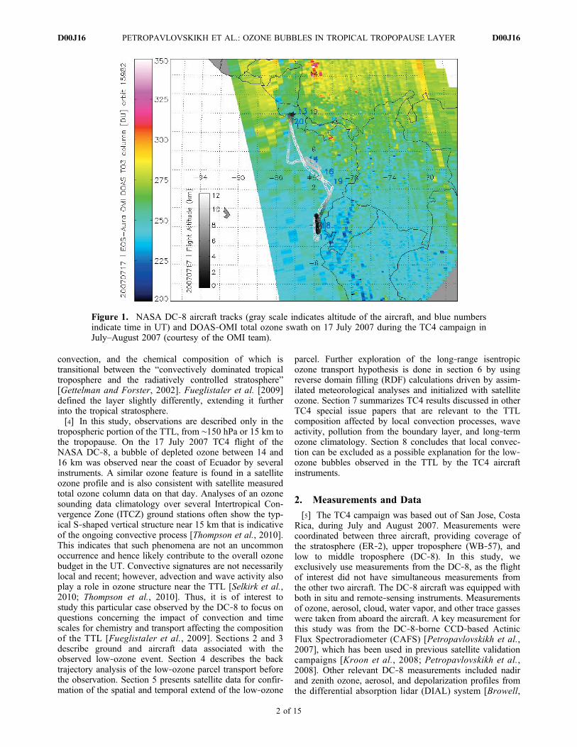
Figure 2. Ozone column data time series are shown for the NASA DC‐8 flight on 17 July 2007. Thecoincident OMI‐TOMS version 2.2 total ozone column data above the clouds (magenta) and above thesurface (blue) are plotted for comparison with the combined CAFS total ozone column (black): a com-bination of the CAFS‐derived ozone column above (green) and the climatological ozone column below(orange; offset by 150 DU) the NASA DC‐8 aircraft level. The approximate time of the low‐ozone valueencounter (at 1700 UT) is marked by the red vertical line. The dashed vertical line marks the Aura satelliteoverpass time at 1930 UT.


3 of 15

tracks. Figure 2 shows time series of CAFS ozone columns(green) derived above the altitude of the DC‐8 for the 17 July2007 flight. In addition, the colocated OMI‐TOMS version2.2 data are shown as total ozone column above the clouds(magenta) and ozone columns above the surface (blue). Thedepleted ozone column (by ∼10 DU) above the DC‐8 air-craft is found at about 1700 UT (Figure 2, vertical red line).The extension of the CAFS‐derived partial ozone columndata (green) with ozone climatology [Bhartia and Wellemeyer,2002] estimated below the DC‐8 altitude (orange) createsa total ozone column data set (black symbols) that matches asimilar reduction in the OMI‐TOMS total ozone columntime series (seen in both blue and magenta symbols). Itsuggests that the reduction in OMI‐TOMS total ozone col-umn is entirely confined to the altitudes above the aircraft.

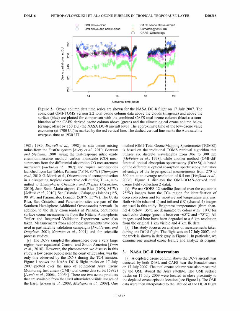
[10] This anomaly in the CAFS and OMI ozone columnobservations occurs at the same time that the DIAL verticalprofile data shows a bubble of depleted ozone between 14and 16 km. Figure 3 shows the cross‐section contour plotof the aerosol scattering ratio (a) and ozone mixing ratio(b) distributions above and below the aircraft level asmeasured by the DIAL system during the part of the flightbetween 1600 and 1720 UT. This portion of the flight wasflown at an altitude of 11.3 km (until about 1702 UT whenthe aircraft turned and descended to 10.3 km altitude). Theblack line in the middle of Figure 3a indicates the DC‐8 altitude. Note that FastOz in situ ozone data are includedin Figure 3b and are shown as a color‐coded thin line at thealtitude of the NASA DC‐8 aircraft. The ozone anomalybetween 14 and 16 km altitude is measured twice in DIAL

Figure 3. Cross sections of the (a) aerosol scattering ratio at 1064 nm and (b) ozone mixing ratio (ppbv)from the DIAL instrument onboard the NASA DC‐8 flight on 17 July 2007 are shown above and belowthe aircraft level, and along the flight track. The colors indicate different levels of aerosol scattering andozone mixing ratios, whereas respective color legends are provided next to each panel. Two depletedozone bubbles between ∼14 and 16 km are marked with black ovals. The corresponding latitude and lon-gitude coordinates of the DC‐8 platform are also provided at the bottom of both plots. The black line inthe middle of the Figure 3a indicates the DC‐8 altitude. A color‐coded thin line at the altitude of theNASA DC‐8 aircraft in the middle of Figure 3b represents the FastOz in situ ozone mixing ratio data.


4 of 15

time series (centered around 1653 UT on the southboundleg and again around 1705 on a parallel track heading north0.4° longitude farther to the west). The temporal extensionof the low‐ozone feature is about 12 min (for both epi-sodes). The NASA DC‐8 cruises with a true air speedbetween 787 and 908 km/h (or between 425 and 490 knots).The DC‐8 speed was recorded at ∼821 km/h during thelow‐ozone bubble encounter. Therefore, the transversedimension of the detected air mass can be estimated at∼165 km. The variation in ozone noted here is approxi-mately a factor of 2, from a high value in the 15 km regionof ∼0.125 ppmv (or 125 ppb) to a low value of ∼0.06 ppmv(60 ppb). To estimate the partial column of ozone between14 and 16 km, we use basic profile information from theozonesonde launched at San Cristobal, Galapagos Islands(1°S, 90°W that is in relatively close vicinity to the low‐ozone air mass location at ∼2°S, 82°W) on 16 July 2007.That sonde recorded ∼154 and ∼110 hPa air pressure at 14and 16 km altitude, respectively. Assuming ozone is wellmixed in that altitude range, as indicated by the DIALcurtain, and using the 60 ppbv difference between the low‐ozone feature and the background measured by the DIALinstrument at 15 km, we thus estimate a partial columnozone reduction of ∼2 DU. Therefore, it appears to be about20% of the 10 DU reduction detected in both the CAFSpartial and OMI total column ozone data (Figure 2) whilecrossing the area with low‐ozone air mass. There has to bean additional ozone decrease, possibly related to the dif-ference in the tropopause altitude in the area of ozonebubble compared to the climatological mean.[11] To determine the origin of the ozone anomaly at 15

km altitude, the coincident in situ ozone measurements wereexamined for signs of the local deep convection at 11.3 kmflight level. In situ ozone measurements were collected bythe FastOz instrument [Avery et al., 2010] aboard the DC‐8.During most of this flight, an average 38 ± 6 ppbv of ozone

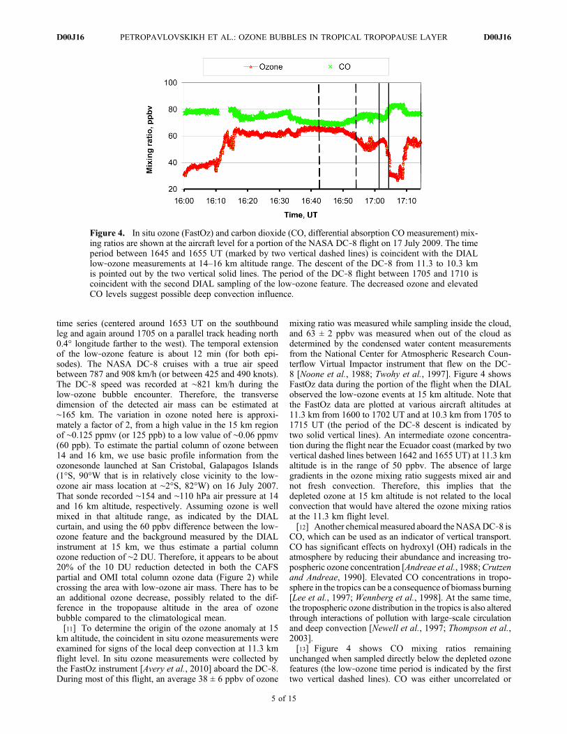
mixing ratio was measured while sampling inside the cloud,and 63 ± 2 ppbv was measured when out of the cloud asdetermined by the condensed water content measurementsfrom the National Center for Atmospheric Research Coun-terflow Virtual Impactor instrument that flew on the DC‐8 [Noone et al., 1988; Twohy et al., 1997]. Figure 4 showsFastOz data during the portion of the flight when the DIALobserved the low‐ozone events at 15 km altitude. Note thatthe FastOz data are plotted at various aircraft altitudes at11.3 km from 1600 to 1702 UT and at 10.3 km from 1705 to1715 UT (the period of the DC‐8 descent is indicated bytwo solid vertical lines). An intermediate ozone concentra-tion during the flight near the Ecuador coast (marked by twovertical dashed lines between 1642 and 1655 UT) at 11.3 kmaltitude is in the range of 50 ppbv. The absence of largegradients in the ozone mixing ratio suggests mixed air andnot fresh convection. Therefore, this implies that thedepleted ozone at 15 km altitude is not related to the localconvection that would have altered the ozone mixing ratiosat the 11.3 km flight level.[12] Another chemical measured aboard theNASADC‐8 is

CO, which can be used as an indicator of vertical transport.CO has significant effects on hydroxyl (OH) radicals in theatmosphere by reducing their abundance and increasing tro-pospheric ozone concentration [Andreae et al., 1988;Crutzenand Andreae, 1990]. Elevated CO concentrations in tropo-sphere in the tropics can be a consequence of biomass burning[Lee et al., 1997; Wennberg et al., 1998]. At the same time,the tropospheric ozone distribution in the tropics is also alteredthrough interactions of pollution with large‐scale circulationand deep convection [Newell et al., 1997; Thompson et al.,2003].[13] Figure 4 shows CO mixing ratios remaining

unchanged when sampled directly below the depleted ozonefeatures (the low‐ozone time period is indicated by the firsttwo vertical dashed lines). CO was either uncorrelated or

Figure 4. In situ ozone (FastOz) and carbon dioxide (CO, differential absorption CO measurement) mix-ing ratios are shown at the aircraft level for a portion of the NASA DC‐8 flight on 17 July 2009. The timeperiod between 1645 and 1655 UT (marked by two vertical dashed lines) is coincident with the DIALlow‐ozone measurements at 14–16 km altitude range. The descent of the DC‐8 from 11.3 to 10.3 kmis pointed out by the two vertical solid lines. The period of the DC‐8 flight between 1705 and 1710 iscoincident with the second DIAL sampling of the low‐ozone feature. The decreased ozone and elevatedCO levels suggest possible deep convection influence.


5 of 15

anticorrelated with ozone during most of the flight. The lackof the elevated CO concentrations in the upper tropospherebefore 1705 UT, while high concentration (∼90 ppbv) levelswere measured near the surface (spiral portion of the DC‐8 flight between ∼1720 and 1840 UT; data not shown),suggests that DC‐8‐sampled air mass at 11.3 km was dif-ferent from the polluted marine boundary layer. Below theDIAL‐detected ozone minimum at ∼15 km, FastOz instru-ment measurements show an intermediate ozone concen-tration in the range of 50 ppbv, which suggests mixed air.The period of the DC‐8 flight between 1705 and 1710 iscoincident in time with the second DIAL sampling of thelow‐ozone feature (between the second solid vertical lineand the right edge of the plot) where an ozone minimum of30 ppbv coincides with elevated CO readings. This periodoccurs right after a short descent from 11.3 to 10.3 km(indicated by two solid lines), which suggests possibleconvective influence at the DC‐8 aircraft level. Since theDC‐8 was at a lower altitude and different longitude for thesecond pass, it likely encountered different dynamicalconditions. Although high clouds were seen in the nadir‐looking DIAL aerosol channel (with cloud top heights justbelow 10 km) up to 1642 UT and after 1705 UT (Figure 3a),the satellite images near the time of the aircraft flight do notindicate any deep convection reaching up to the 14–16 kmlevels (see section 4 for more discussion). The depletedozone at the NASA DC‐8 level appears to be a narrow layerlocated above the cloud tops and just above a slightenhancement in the DIAL nadir aerosol image (Figure 3a).The aircraft seemed to intercept the upper outer fringe of thislayer at 1657 UT but was on the lower outer fringe when itleveled out at 10.3 km at 1705 UT. There could very likelybe the influence of shallower convection at the DC‐8 levels,with the possibility of transport from the east (see section 4on back trajectories), but that convection is not getting up tothe levels where the depleted ozone is detected. Moreover,the DIAL data show a break in the vertical distribution withincreased ozone mixing ratios at 13 km (Figure 3b).Therefore, the CO observations at the NASA DC‐8 aircraftflight level provide supporting evidence that the depletedozone is not related to local vertical transport.

4. Back Trajectory Analysis of the Low‐OzoneAir Mass

[14] In this study, backward trajectory calculations andsatellite data are analyzed to examine the evolution andidentify the likely source region of the low‐ozone air massobserved from the DC‐8 on the 17 July flight. Back tra-jectories are started at the geo‐location and time of the DC‐8 DIAL interception of the low‐ozone bubble event (nearthe Ecuador coast (3°S, 82°W) between 1630 and 1700 UT).[15] At first, following the approach of Pfister et al.

[2001, 2010], a combination of National Center for Envi-ronmental Prediction (NCEP) reanalysis meteorologicalfields and GOES images were used to create convectiveinfluence plots for the area under question [Pfister et al.,2001]. The back trajectories were run for 8 days beforethe event on 17 July 2007 and were stopped when it wasdetermined that parcel had encountered convection as notedon the satellite images. The geo‐location of the air parcelswas checked against the GOES images for bright clouds (see

Figures 6 and 7) that are indicative of deep convectionevents. The brightness temperatures were also adjusted by asmuch as 6° according to the findings of Sherwood et al.[2004] and Minnis et al. [2008]; details regarding this cor-rection are given by Pfister et al. [2010]. Whenever a backtrajectory parcel was found to be at least as high as thealtitude of the intercepted cold cloud, it was considered to beconvectively influenced [Pfister et al., 2010]. For example,Figure 5 shows the GOES‐12 satellite IR image at 1745 UTtaken on 17 July 2007. The Aura High Resolution DynamicsLimb Sounder (H), Tropospheric Emission Spectrometer (+),andMicrowave Limb Sounder/OzoneMonitoring Instrument(M) instrument sampling tracks are also shown. IR channel 4typically “sees” the surface unless it is obstructed by clouds.In this and subsequent images, brightness temperaturesbelow −35°C have been marked with bright green colorsrepresenting the area of deep convection. The three mostprominent areas of deep convection are found in IR imagesover the Pacific coast of Mexico, Panama, and northernSouth America. Moreover, based on the DIAL ozone curtainplots (Figure 3), it appears that the depleted ozone is foundbetween about 14.9 km (or ∼49 kft) and 15.7 km (or ∼52 kft)geometric altitude. Therefore, the lower limit for trajectorieswas placed at a pressure of 134 hPa, while the upper limit wasextended to 117 hPa.[16] Additional tests were performed to investigate sen-

sitivity of the back trajectory analysis to the meteorologicaldata fields and transport assumptions. For the analysis pre-sented in Figures 5–7, 10 day back trajectory calculationswere performed using the HYbrid Single‐Particle Lagrang-ian Integrated Trajectory (HYSPLIT) model [Draxler andHess, 1997, 1998; Draxler, 2003]. The input meteorologi-cal data for HYSPLIT were selected from the NCEP GlobalData Assimilation System (GDAS) (1° × 1° resolution;http://www.emc.ncep.noaa.gov/modelinfo/index.html)model output. Isentropic back trajectories were initialized at1700 UT on 17 July 2007 over a matrix of nine latitudes andeight longitudes spanning the bounding latitude/longitudebox of the region over which the DC‐8 observed the low‐ozone bubble (near the Ecuador coast (3°S, 82°W) between1630 and 1700 UT). Additional kinematic model runs (datanot shown) were performed using combinations of theGDAS omega (vertical velocity in pressure coordinates) aswell as different initialization times (1600 and 1800 UT) toinvestigate the sensitivity of the results. Although the endpoints of these runs differ slightly from the nominal run, theresults below are not sensitive to these small perturbations ininitialization time or vertical velocity used in the analysis.The similarity between the adiabatic and omega trajectoriespoints to the relative insignificance of diabatic heating onthe trajectory of the low‐ozone parcel within the TTL overthe time scale considered here. A complementary view isthat vertical velocities and vertical wind shear in the TTL aresmall compared to other regions of the troposphere, andhence have little effect on the trajectory end points over theperiod of 1 week. In addition, the trajectories were stoppedwhenever the convective influence analyses (describedabove) suggested the intercept with the deep convectivesystem.[17] Figure 5 shows the back trajectory runs initialized at

the altitude of the low‐ozone bubble (top, 15.4 km) and atthe mean altitude of the DC‐8 during the low‐ozone bubble


6 of 15

measurement (bottom, 10.4 km). The backward trajectoryanalysis plots illustrate that the air masses at the DC‐8 alti-tude and 15 km are of significantly different origin, with theflight‐level air mass originating from the east over SouthAmerica and the 15 km air mass originating from the westand ultimately north‐northeast over the Panama Bightregion.[18] The 15 km back trajectories were tracked backward

in time to the point at which they horizontally interceptedconvection in the GOES channel 4 imagery (defined by lowbrightness temperatures <238 K, or blue colors in theFigures 5–7) to obtain a qualitative understanding of wherethe trajectories likely originated. In addition, they were also

checked for consistency with the above described analysisof the convectively influenced parcels [Pfister et al., 2001,2010]. As the trajectories make their turn and head north, wefind convective influence in the time range >5 days old. Alltrajectories intercepted convection between 10 and 12 July,5–7 days before being measured by the DC‐8. The south-ernmost trajectories (black through light blue colors)encountered convection in the Panama Bight and East Pacificregion, whereas the northernmost trajectories encounteredconvection off of the east coast of Colombia, over Colombia,and over Venezuela (green through red colors). Although theconvective source of the trajectories at a given initializationlatitude is somewhat sensitive to the start time and vertical

Figure 5. (top) Backward trajectories initialized at the altitude and latitude/longitude of the low‐ozoneair mass (∼15 km) are plotted over the GOES channel 4 brightness temperature imagery taken at 1745 UT(colors from black to red indicate the starting latitude of the trajectory, and diamonds are plotted at 0000UT on each day of the trajectories). The DC‐8 flight track is shown in white. (bottom) Same as the toppanel but for trajectories initialized at the DC‐8 altitude (∼10 km).


7 of 15

transport used (i.e., isentropic trajectories as opposed to thoseincluding assimilated vertical motion output), all of thecombinations of backward trajectories yield convectivesources in the vicinity of Panama and Colombia. Because theGOES brightness temperatures are consistently lower overPanama for the trajectories considered here, we hypothesizethat the low‐ozone bubble air mass originated over thisregion. Overall, these back trajectories support the idea thatlow‐ozone air detrained from deep convection over theSouth and Central America regions can be transportedthrough the TTL over long times (∼7 days) and distances(∼1000 km) in a coherent manner.

[19] Detailed analyses of ozone soundings during the TC4campaign period are presented by Thompson et al. [2010].They find that between 40% and 50% of ozone in the TTL isinfluenced by convective transport. For example, Figure 3bin that paper [Thompson et al., 2010] presents ozonesondemeasurements at the Las Tables, Panama, site during theTC4 campaign. The mean ozone mixing ratio between the 3and 10 km altitude range (active convection zone accordingto the study by Avery et al. [2010]) is about 50 ± 10 ppbv.Since the average mixing ratio in the DIAL‐measured low‐ozone bubble is about 60 ± 10 ppbv, we can expect that

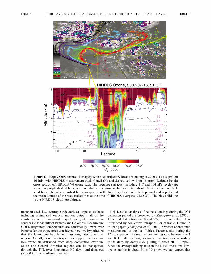
Figure 6. (top) GOES channel 4 imagery with back trajectory locations ending at 2200 UT (+ signs) on16 July, with HIRDLS measurement track plotted (Hs and dashed yellow line). (bottom) Latitude‐heightcross section of HIRDLS V4 ozone data. The pressure surfaces (including 117 and 134 hPa levels) areshown as purple dashed lines, and potential temperature surfaces at intervals of 10° are shown as blacksolid lines. The yellow dashed line corresponds to the trajectory location in the top panel and is plotted atthe mean altitude of the back trajectories at the time of HIRDLS overpass (2120 UT). The blue solid lineis the HIRDLS cloud top altitude.


8 of 15

∼20% of the mixing might have occurred in the air mass thatwas transported through the UT during convection.

5. Satellite Observations

[20] In support of our hypothesis of long‐range transportfrom the Panama region, we present data from the twocoincident times over the course of the 10 day trajectories inwhich the air parcels were located in the proximity of AuraHigh Resolution Dynamics Limb Sounder (HIRDLS) mea-surements [Gille et al., 2008; Khosravi et al., 2009]. Thetrajectory locations over the GOES IR imagery are shown inFigures 6 (top) and 7, whereas latitude cross sections ofHIRDLS ozone data for the first time segment are shown inFigure 6 (bottom).[21] The HIRDLS V4 ozone profile data cover a wider

range of latitudes, while profiles are about 100 km apart, soits resolution does not contain the fine horizontal detailsobserved by DIAL. However, the vertical resolution ofHIRDLS is about 1 km, which should be sufficient foridentifying the vertical ozone gradient. The HIRDLS ozonepressure‐latitude cross section is shown in Figure 6 (bot-tom). It is accompanied by the GOES IR images and tra-jectories shown in Figure 6 (top). Yellow arrows and thevertical dashed line in Figure 6 (top) point to the trajectorylocations on 16 July over the eastern Pacific ocean, far fromthe regions of persistent convection off the coasts of CentralAmerica. Also, a region of low‐ozone air close in space andtime to the altitude of the back trajectories (∼15.25 km) ispresent in the HIRDLS data taken at ∼2120 UT (Figure 6,bottom, yellow horizontal line and arrows). Because of thelack of convective clouds in this region of low ozone, asevidenced by the absence of cold colors in the GOESimagery (Figure 6, top), we hypothesize that this low‐ozoneregion in the HIRDLS data is the same air mass measuredon 17 July by the DC‐8. The plotted HIRDLS data havebeen screened as recommended by the HIRDLS data doc-ument (HIRDLS Data Description and Quality Document,http://disc.sci.gsfc.nasa.gov/Aura/data‐holdings/HIRDLS/hirdls2_004.shtml); this includes eliminating data pointswith negative precision flags (which are dominated by a

priori information) and data points earthward of the detectedcloud top pressure. The region to the south of the trajectorylocation (between 10°S and 5°S) and below 17 km where nodata exist (Figure 6, white) may be due to the presence ofclouds or when a retrieval error covariance becomes greaterthan half of the a priori error covariance [Nardi et al., 2008].However, the deep gradient in the HIRDLS ozone profilesbetween 2°S and 5°S latitude and between ∼13 and 17 kmaltitude shows the depleted ozone area coincident withlocation of the transported low‐ozone bubble as suggestedby our back trajectory analysis.[22] Figure 7 shows the trajectory locations at 2100 UT on

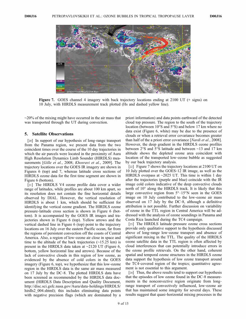
10 July plotted over the GOES‐12 IR image, as well as theHIRDLS overpass at ∼2025 UT. This time is within 1 dayafter the trajectories (purple and blue) coincide with the IRimage cold colors indicative of the deep convective cloudsnorth of 10° along the HIRDLS track. It is likely that thislarge convective region from 5°–15°N seen in the GOESimage on 10 July contributed to the low‐ozone air massobserved on 17 July by the DC‐8, although a definitiveattribution is not possible. Further discussion on variabilityof ozone in the TTL region in Central America will be ad-dressed with the analysis of ozone soundings in Panama andCosta Rica launched during the TC4 campaign.[23] The HIRDLS latitude‐pressure ozone cross sections

provide only qualitative support to the hypothesis discussedabove of long‐range low‐ozone transport and absence ofsignificant mixing in the TTL. The quality of the HIRDLSozone satellite data in the TTL region is often affected bycloud interferences that can potentially introduce errors inthe ozone profile retrievals. On the other hand, coherentspatial and temporal ozone structures in the HIRDLS ozonedata support the hypothesis of low ozone transport aroundthe TC4‐covered region of the tropics; quantitative agree-ment is not essential to this argument.[24] Thus, the above results tend to support our hypothesis

that the episodes of low ozone found in the DC‐8 measure-ments in the nonconvective region originate from long‐range transport of convectively influenced, low‐ozone airthat has maintained some integrity for several days. Theseresults suggest that quasi‐horizontal mixing processes in the

Figure 7. GOES channel 4 imagery with back trajectory locations ending at 2100 UT (+ signs) on10 July, with HIRDLS measurement track plotted (Hs and dashed yellow line).


9 of 15

upper tropical troposphere are relatively slow. Deep con-vection over Panama is likely the source of the observedlow‐ozone “bubble” (see further discussion of ozonesounding data).

6. RDF Analysis

[25] The back trajectory analysis discussed above sug-gested the possibility of the long‐range quasi‐horizontaltransport of a low‐concentration ozone bubble detected bythe DIAL and CAFS instruments between 14 and 16 kmnear the Ecuador coast from the Panama‐Bight region,where it was generated by the deep convection mechanism.The DIAL and CAFS instruments detected a low‐ozonebubble between 14 and 16 km altitude around 1700 UTduring the NASA DC‐8 aircraft flight on 17 July 2007. Herewe explore the long‐range transport hypothesis further byusing reverse domain filling calculations [Manney et al.,1998; Sutton et al., 1994] driven by GEOS‐5 data assimi-lation system meteorological analyses [Reinecker et al.,2008] and initialized with Aura Microwave Limb Sounder(MLS) data [Waters et al., 2006] to infer the isentropictransport of ozone features noted here.[26] For this analysis, trajectory calculations using

assimilated winds from the GEOS‐5 analysis were startedon a dense grid (0.25° latitude by 0.40° longitude) at severalisentropic levels and run back 8 days; at that time, griddedMLS (or HIRDLS) data were interpolated to the parcel lo-cations to provide an estimate of the ozone that was trans-ported to the starting locations of the trajectories. A secondset of similar calculations was done, but with the parcelsinitialized on a dense vertical grid (100 levels equallyspaced in log‐potential temperature between 330 and 530 K)at the 5 minute average positions of the aircraft flight track.Thus, the RDF maps/profiles are based on transport byGEOS‐5 winds and initialization with a single day ofgridded MLS data. Calculations were also initialized withHIRDLS V4 ozone data and generally showed similar resultsto those initialized with MLS data; since the MLS version 2.2data are better characterized in the Upper Troposphere/LowerStratosphere (UTLS) [Livesey et al., 2008] and are lessfrequently affected by clouds than HIRDLS, we show onlythe MLS results here. Comparable results were obtainedusing preliminary version 3 MLS data. Calculations initial-ized with equivalent latitude [Butchart and Remsberg, 1986]also provide a consistent picture of the air parcels’ origins.While the MLS (and to a lesser degree, HIRDLS) fields usedfor initialization have much coarser horizontal and verticalresolution than the RDF grids, previous studies using similardata sets [Manney et al., 1998, 2000, and references therein]have demonstrated good skill in reproducing small‐scalefeatures in observed profiles that result from differentialadvection by the large‐scale wind fields.[27] Figure 8a shows RDF ozone from an MLS‐initialized

run, which shows low‐ozone features at locations consistentwith where the DC‐8 sampled low‐ozone bubbles nearEcuador on 17 July 2007. The feature also appears at 360 K,consistent with the vertical extent of the low‐ozone bubblein the aircraft observations (G.M.). Gradients comparableto those observed from the DC‐8 are seen in the RDF‐generated ozone field, indicating that transport over 8 dayscan indeed generate features like those observed. RDF cal-

culations were also initialized with several other chemicalspecies measured by MLS (H2O, CO, and HNO3; results arenot shown); these show strong consistency in the morphol-ogy of the RDF fields with those for ozone, suggesting thatthe RDF calculations are largely showing transport of realatmospheric features, since transported “noise” (i.e., spuriousvalues) would be less likely to be correlated among all thespecies.[28] Results in Figure 8a suggest that the low‐ozone

feature in the RDF analysis near the coast of Ecuador at the360 K potential temperature level (near 15 km altitude; seeFigure 3) are similar to the DIAL‐observed low‐ozonemixing ratios between 14 and 16 km altitude. The lightblue‐colored filament of ozone that represents the low‐ozone mixing ratio of 50 ppbv extends to the west from theEcuador coast (DC‐8 tracks are marked by the white line),loops under the red‐colored (higher mixing ratio) ozonefeature in the middle of the plot, and then extends to thenorth up to the coast of Mexico. The vertical extend ofozone feature may be smoothed out because of the initiali-zation with MLS ozone profiles that have low vertical,horizontal, and temporal resolution, but it is still indicativeof the transport‐related ozone residuals between 14 and16 km altitude.[29] Results of an RDF analysis “transporting” equivalent

latitude [Butchart and Remsberg, 1986] are shown inFigure 8b. The equivalent latitudes are the latitudes thatwould enclose the same area as the potential vorticity con-tours, thus showing at what equivalent latitude the air at eachpoint in the plot originated 8 days previously. The light sand‐colored filaments seen near the south end of the DC‐8 flighttrack (shown as a white line) suggest that the low‐ozonebubble most likely originated at about 10°N. The RDFanalyses support our hypothesis of the origination of the low‐ozone bubble in the ITCZ as the region of the deep con-vective processes at low northern latitudes.[30] Finally, MLS‐initialized RDF calculations on the

dense vertical grid were used to produce a cross sectionsimilar to Figure 3, albeit with much coarser time resolution.Figure 8c shows time‐altitude distribution of the ozonemixing ratio from the RDF analysis (described above) that isadjusted by 25 ppbv to match the ozone range in Figure 3.Results are plotted between 340 and 375 K potential tem-perature levels and between 1600 and 1720 UT range that issimilar to the spatial and temporal distribution of the DIALozone mixing ratio measured aboard the NASA DC‐8 flighton 17 July 2007 (Figure 3b). Distinct ozone minima are seennear 365 K at approximately the times the ozone bubbleswere sampled by the aircraft. The lowest ozone in the RDFcalculations occurs slightly earlier in time along the flighttrack than observed. This is likely related to the coarse timeresolution in the RDF calculations, but the low‐ozone fea-ture is apparent during the entire period it was observed bythe aircraft. The vertical position and extent of the featureare very close to those in the aircraft observations. RDFcalculations were also done using HIRDLS data; however,because of data quality issues (section 5), HIRDLS coveragebelow ∼370 K is insufficient for the initialization. AHIRDLS RDF section similar to Figure 8c shows a hint of alow‐ozone feature just below 370 K, consistent with theMLS‐derived feature in Figure 8c. Note that layers ofenhanced ozone are seen both above and below the simu-


10 of 15

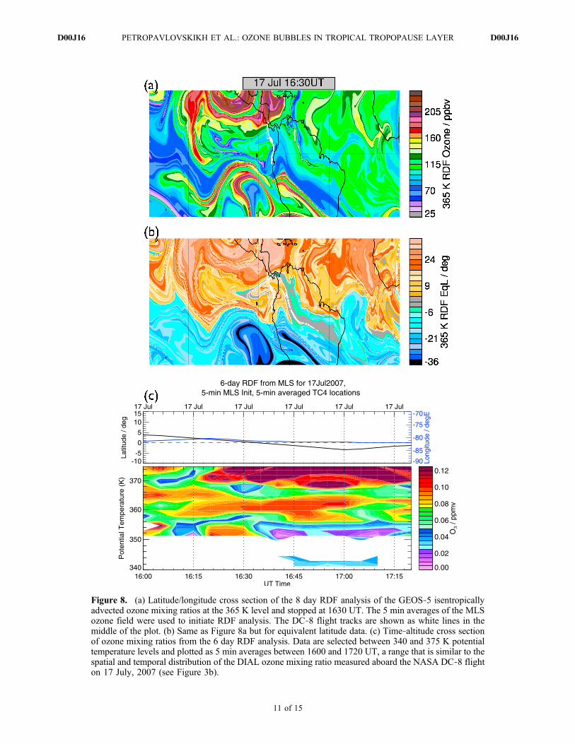
Figure 8. (a) Latitude/longitude cross section of the 8 day RDF analysis of the GEOS‐5 isentropicallyadvected ozone mixing ratios at the 365 K level and stopped at 1630 UT. The 5 min averages of the MLSozone field were used to initiate RDF analysis. The DC‐8 flight tracks are shown as white lines in themiddle of the plot. (b) Same as Figure 8a but for equivalent latitude data. (c) Time‐altitude cross sectionof ozone mixing ratios from the 6 day RDF analysis. Data are selected between 340 and 375 K potentialtemperature levels and plotted as 5 min averages between 1600 and 1720 UT, a range that is similar to thespatial and temporal distribution of the DIAL ozone mixing ratio measured aboard the NASA DC‐8 flighton 17 July, 2007 (see Figure 3b).


11 of 15

lated low‐ozone bubbles. The combination of RDF mapsand cross sections suggests that the low‐ozone bubbles are,in fact, the result of sampling across the narrow dimensionof long streamers of ozone transported relatively intact overlong distances and times. Note that the RDF calculations, bydefinition, include no mixing; the reasonable reproductionof the observed low‐ozone bubbles in the RDF fields is thusan additional indication that the air comprising them hasbeen transported over long distances with little mixing.

7. Discussion

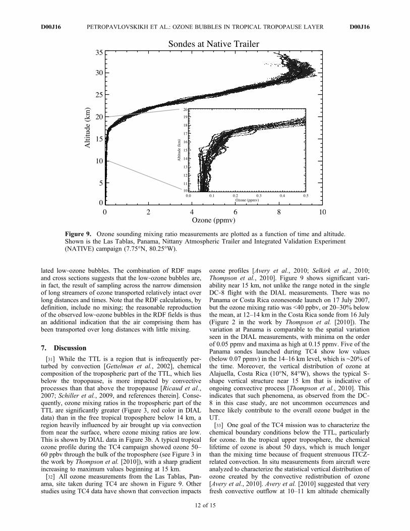
[31] While the TTL is a region that is infrequently per-turbed by convection [Gettelman et al., 2002], chemicalcomposition of the tropospheric part of the TTL, which liesbelow the tropopause, is more impacted by convectiveprocesses than that above the tropopause [Ricaud et al.,2007; Schiller et al., 2009, and references therein]. Conse-quently, ozone mixing ratios in the tropospheric part of theTTL are significantly greater (Figure 3, red color in DIALdata) than in the free tropical troposphere below 14 km, aregion heavily influenced by air brought up via convectionfrom near the surface, where ozone mixing ratios are low.This is shown by DIAL data in Figure 3b. A typical tropicalozone profile during the TC4 campaign showed ozone 50–60 ppbv through the bulk of the troposphere (see Figure 3 inthe work by Thompson et al. [2010]), with a sharp gradientincreasing to maximum values beginning at 15 km.[32] All ozone measurements from the Las Tablas, Pan-

ama, site taken during TC4 are shown in Figure 9. Otherstudies using TC4 data have shown that convection impacts

ozone profiles [Avery et al., 2010; Selkirk et al., 2010;Thompson et al., 2010]. Figure 9 shows significant vari-ability near 15 km, not unlike the range noted in the singleDC‐8 flight with the DIAL measurements. There was noPanama or Costa Rica ozonesonde launch on 17 July 2007,but the ozone mixing ratio was <40 ppbv, or 20–30% belowthe mean, at 12–14 km in the Costa Rica sonde from 16 July(Figure 2 in the work by Thompson et al. [2010]). Thevariation at Panama is comparable to the spatial variationseen in the DIAL measurements, with minima on the orderof 0.05 ppmv and maxima as high at 0.15 ppmv. Five of thePanama sondes launched during TC4 show low values(below 0.07 ppmv) in the 14–16 km level, which is ∼20% ofthe time. Moreover, the vertical distribution of ozone atAlajuella, Costa Rica (10°N, 84°W), shows the typical S‐shape vertical structure near 15 km that is indicative ofongoing convective process [Thompson et al., 2010]. Thisindicates that such phenomena, as observed from the DC‐8 in this case study, are not uncommon occurrences andhence likely contribute to the overall ozone budget in theUT.[33] One goal of the TC4 mission was to characterize the

chemical boundary conditions below the TTL, particularlyfor ozone. In the tropical upper troposphere, the chemicallifetime of ozone is about 50 days, which is much longerthan the mixing time because of frequent strenuous ITCZ‐related convection. In situ measurements from aircraft wereanalyzed to characterize the statistical vertical distribution ofozone created by the convective redistribution of ozone[Avery et al., 2010]. Avery et al. [2010] suggested that veryfresh convective outflow at 10–11 km altitude chemically

Figure 9. Ozone sounding mixing ratio measurements are plotted as a function of time and altitude.Shown is the Las Tablas, Panama, Nittany Atmospheric Trailer and Integrated Validation Experiment(NATIVE) campaign (7.75°N, 80.25°W).


12 of 15

more closely resembles in situ ozone sampled at about 3 kmthan it does at the surface, with very low variability in themeasurements seen during updrafts. With vertical transporttime scales on the order of 10–20 min, it seems unlikely forstorms to efficiently entrain and mix midtropospheric air.This suggests that vertical transport in the middle tropo-sphere is predominantly from 2–3 to 10–11 km and thatvertical transport is more complicated than just movingboundary layer air up to the tropopause. Evidence from thesondes shows that local convection predominantly impactsozone up to 11 km.[34] For the case we have examined in this work, shortly

after the first encounter of the low‐ozone bubble event, thein situ and DIAL ozone mixing ratio data indicate anintercept of the thin depleted ozone layer located just abovethe deep convective clouds. It suggests the influence ofshallower local convection at the DC‐8 levels at ∼10.3 km,with the possibility of transport from the east. However,DIAL data show a break in vertical distribution withincreased ozone mixing ratios at 13 km. Thus, the localconvection does not reach up to the levels where the low‐ozone bubble is detected. Therefore, the depleted ozone at14–16 km was not the result of local uplift. The back tra-jectory runs indicate that the low‐ozone features observedby DIAL were the result of deep convective upwelling in theITCZ, followed by quasi‐horizontal transport to south of theequator. It is somewhat surprising that the low‐ozone fea-tures were so pronounced after moving around the UT for≥1 week, which may reveal information on mixing timescales in the TTL. Our results are confined to assessingmixing times from our limited trajectories; in this case, wewould infer mixing times greater than 1 week, which is notinconsistent with the results of James and Legras [2009].[35] Evidence for low‐ozone bubbles is limited. In the

DC‐8 flights, the transit from California to Costa Rica alsoshowed evidence of a thin low‐ozone layer above theprincipal convective outflow signal that is very prominentaround 10 km (Figure 6b in the work of Thompson et al.[2010]). Indeed, analysis of wave signatures by Thompsonet al. [2010] in the Panama soundings reveals both con-vective and advective flows affect ozone structure in theTTL. Unfortunately, very few TC4 flights were able tomeasure the TTL ozone outside of the convectively influ-enced region near the Panama Bight and without majorcloud interference. However, such low‐ozone values in theTTL between 14 and 16 km have been observed in pastexperiments; low‐ozone values in the TTL were seen inDIAL data during the Pacific Exploratory Mission A (PEM‐A) and PEM‐B campaigns [Browell et al., 2001, 2003].However, it should be noted that the previous observationsdid not observe a similar, spatially coherent (∼2 km thick invertical and ∼100 km long in horizontal dimensions) low‐ozone “blob” such as seen during TC4. Because of thewinds in this case, there is a contribution from convectionthat is north of the equator and likely from the Panama Bightregion.[36] Some other points may be useful for further discus-

sion. For example, the DIAL ozone data on 17 July at 1710UT show large ozone values just below the ozone bubble,larger than at similar altitudes on either side of the low‐ozone area. High‐ozone air parcels likely have stratosphericorigin, either via local vertical exchange or quasi horizontal

exchange across the subtropical jet. Because the vertical andhorizontal winds at the TTL levels were very slow, quasi‐horizontal transport from higher latitudes is the likely causefor the high ozone layer. This is supported by the RDFcalculations, which showed alternating narrow layers ofhigh and low ozone resulting from isentropic transport.[37] There are other possibilities we have considered that

could have caused the low‐ozone features noted above 14 kmon 17 July in the DIAL measurements. The DC‐8 was flyingin close proximity to the volcanic outflow from Ecuador. Thechemical reaction involving volcanic SO2→H2SO4 particlescould be the reason for the ozone destruction through theactivation of chlorine. However, if that were the case, wewould expect to see aerosols present in the low‐ozone airmass. The contours in Figure 3 show aerosols in the regionsof elevated ozone in the 14–16 km levels, indicative of anaged air mass, but there are no aerosols detected by DIAL inthe low‐ozone bubble, hence supporting the idea that it is arelatively “freshly” pumped up air mass.[38] Yet another mechanism of ozone destruction could be

related to the combination of high H2O mixing ratios andoccurrence of clouds below (apparent from backscatter inDIAL aerosol backscatter data). It could lead to high pho-tochemical destruction of ozone through photochemical lossJ(O3)→O(1D) + H2O→OH, followed by additional ozoneloss through the HO2/OH catalytic cycle. However, theDIAL/LASE system did not detect high mixing water vaporabove the DC‐8 level, negating this possibility. Moreover,NO abundance in the UTLS is high enough for supportingozone production mechanism and thus negating the ozoneloss processes. Therefore, enhancements in HOX tend toimprove chemical ozone production even further.

8. Conclusions

[39] To summarize, based on our back trajectory analysis,Figure 5 (top) shows that the coherent low‐ozone bubbleobserved in the south part of the DC‐8 flight of 17 July 2009by the DIAL instrument at ∼1700 UT between 14 and 16 km(Figure 3, green) most likely resulted from nonlocal con-vection occurring near Panama. Supporting evidence for thenonlocality and subsequent transport comes from the factthat a low‐ozone region crossing the back trajectories is seenin satellite observations in the absence of convection severaldays after the convective event (Figure 6). There is a distinctdifference in the direction of trajectories derived aboveaircraft level (Figure 5, top) and at aircraft level (Figure 5,bottom, South America), also supporting the nonlocality ofthe source. Therefore, ozone depletion above the aircraft andelevated/reduced ozone mixing ratios at the aircraft level,and increased ozone below the aircraft, are governed bydifferent processes. The picture of complementary convec-tive and advective influences on ozone structure in the UTand the TTL is consistent with analysis based on wavepatterns in the ozone sounding data over Panama and CostaRica during the TC4 campaign [Thompson et al., 2010].

[40] Acknowledgments. This work was supported by the NASAHeadquarters Atmospheric Composition Focus Area including the UpperAtmospheric Research Program (Michael Kurylo, program manager), theRadiation Science Program (Hal Maring, program manager), and the Tro-


13 of 15

pospheric Chemistry Program (Jim Crawford, program manager). Wegratefully acknowledge helpful discussions with R. McPeters (NASA,Goddard), K. Chance (Harvard University), and E. Hilsenrath (NASAHeadquarters). We also emphasize the crucial contributions of the pilotsand crew of the NASA DC‐8 aircrafts. We extend our gratitude to mis-sion scientists (Brian Toon and Dave Starr) and DC‐8 platform scientists(Mark Schoeberl and Paul Wennberg) for planning and successfully exe-cuting the TC4 campaign. We greatly appreciate support from the AuraHIRDLS, OMI, and MLS teams for providing us with the coincident data.We extend our special thanks to J. Gille and S. Karol (HIRDLS, NCAR)for help with data quality, analysis, and discussion. We also thank MarcKroon (OMI, KNMI) for help with the OMI DOAS data analysis, up-dates, and conscientious figures. The OMI‐TOMS and OMI‐DOAS totalozone data were obtained from the NASA Goddard Earth Sciences (GES)Data and Information Services Center, home of the GES DistributedActive Archive Center. Work at the Jet Propulsion Laboratory, CaliforniaInstitute of Technology, was done under contract with NASA. We extendspecial thanks to Kurt Severance (NASA, Langley) and William Daffer(NASA, JPL) for help preparing the 3‐D graphics in record short time.Finally, we acknowledge the hard work by Gary A. Morris (ValparaisoUniversity) and Alex Bryan and David Lutz (Valparaiso University un-dergraduates), who were responsible for all 25 ozonesonde launches fromLas Tablas. Without their effort, we would have no balloon data fromPanama.

ReferencesAndreae, M. O., E. V. Browell, G. L. Gregory, R. C. Harriss, G. F. Hill,G. W. Sachse, R. W. Talbot, M. Garstang, D. J. Jacob, and A. L.Torres (1988), Biomass‐burning emissions and associated haze layersover Amazonia, J. Geophys. Res., 93(D2), 1509–1527, doi:10.1029/JD093iD02p01509.

Avery, M. A., et al. (2010), Convective Distribution of Tropospheric Ozoneand Tracers in the Central American ITCZ Region: Evidence from Ob-servations During TC4, J. Geophys. Res., doi:10.1029/2009JD013450,in press.

Bhartia, P. K., and C. W. Wellemeyer (2002), OMI TOMS‐V8 Total O3Algorithm, edited by P. K. Bhartia, pp. 15–31, NASA GSFC, Greenbelt,Md.

Browell, E. V. (1981), Lidar measurements of tropospheric gases, Proc.Soc. Photo. Opt. Instrum. Eng., 286, 79–86.

Browell, E. V. (1989), Differential absorption lidar sensing of ozone, Proc.IEEE, 77(3), 419–432, doi:10.1109/5.24128.

Browell, E. V., S. Ismail, and W. B. Grant (1998), Differential absorptionlidar (DIAL) measurements from air and space, Appl. Phys. B, 67(4),399–410, doi:10.1007/s003400050523.

Browell, E. V., et al. (2001), Large‐scale air mass characteristics observedover the remote tropical Pacific Ocean during March–April 1999: Resultsfrom PEM‐Tropics B field experiment, J. Geophys. Res., 106(D23),32,481–32,501, doi:10.1029/2001JD900001.

Browell, E. V., et al. (2003), Large‐scale ozone and aerosol distributions,air mass characteristics, and ozone fluxes over the western Pacific Oceanin late winter/early spring, J. Geophys. Res., 108(D20), 8805,doi:10.1029/2002JD003290.

Butchart, N., and E. E. Remsberg (1986), The area of the stratosphericpolar vortex as a diagnostic for tracer transport on an isentropic surface,J. Atmos. Sci., 43(13), 1319–1339, doi:10.1175/1520-0469(1986)043<1319:TAOTSP>2.0.CO;2.

Crutzen, P. J., and M. O. Andreae (1990), Biomass burning in the tropics ‐impact on atmospheric chemistry and biogeochemical cycles, Science,250(4988), 1669–1678, doi:10.1126/science.250.4988.1669.

Draxler, R. R. (2003), Evaluation of an ensemble dispersion calculation,J. Appl. Meteorol., 42(2), 308–317, doi:10.1175/1520-0450(2003)042<0308:EOAEDC>2.0.CO;2.

Draxler, R. R., and G. D. Hess (1997), Description of the HYSPLIT_4modeling system, Tech. Memo. ERL ARL‐224, 24 pp., NOAA, SilverSpring, Md.

Draxler, R. R., and G. D. Hess (1998), An overview of the HYSPLIT_4modeling system for trajectories, dispersion and deposition, Aust. Meteorol.Mag., 47(4), 295–308.

Folkins, I., M. Loewenstein, J. Podolske, S. J. Oltmans, and M. Proffitt(1999), A barrier to vertical mixing at 14 km in the tropics: Evidencefrom ozonesondes and aircraft measurements, J. Geophys. Res., 104(D18), 22,095–22,102, doi:10.1029/1999JD900404.

Folkins, I., C. Braun, A. M. Thompson, and J. Witte (2002), Tropical ozoneas an indicator of deep convection, J. Geophys. Res., 107(D13), 4184,doi:10.1029/2001JD001178.

Froidevaux, L., and A. Douglass (2001), Earth Observing System (EOS),20,771 pp., Aura Science Data Validation Plan, NASA Goddard SpaceFlight Cent., Greenbelt, Md.

Fueglistaler, S., A. E. Dessler, T. J. Dunkerton, I. Folkins, Q. Fu, and P. W.Mote (2009), Tropical tropopause layer, Rev. Geophys., 47, RG1004,doi:10.1029/2008RG000267.

Gettelman, A., and P. M. D. Forster (2002), A climatology of the tropicaltropopause layer, J. Meteorol. Soc. Jpn., 80(4B), 911–924, doi:10.2151/jmsj.80.911.

Gettelman, A., M. L. Salby, and F. Sassi (2002), Distribution and influenceof convection in the tropical tropopause region, J. Geophys. Res., 107(D10),4080, doi:10.1029/2001JD001048.

Gettelman, A., et al. (2009), The tropical tropopause layer 1960–2100,Atmos. Chem. Phys., 9(5), 1621–1637, doi:10.5194/acp-9-1621-2009.

Gille, J., et al. (2008), High Resolution Dynamics Limb Sounder: Experi-ment overview, recovery, and validation of initial temperature data,J. Geophys. Res., 113, D16S43, doi:10.1029/2007JD008824.

Highwood, E. J., and B. J. Hoskins (1998), The tropical tropopause, Q. J. R.Meteorol. Soc., 124(551), 1579–1604, doi:10.1002/QJ.49712455121.

IPCC (2001), Climate Change 2001: The Scientific Basis, Contribution ofWorking Group I to the Third Assessment Report of the Intergovernmen-tal Panel on Climate Change, edited by J. T. Houghton et al., CambridgeUniv. Press, New York.

James, R., and B. Legras (2009), Mixing processes and exchanges in thetropical and the subtropical UT/LS, Atmos. Chem. Phys., 9(1), 25–38,doi:10.5194/acp-9-25-2009.

Khosravi, R., et al. (2009), Overview and characterization of retrievals oftemperature, pressure, and atmospheric constituents from the High Res-olution Dynamics Limb Sounder (HIRDLS) measurements, J. Geophys.Res., 114, D20304, doi:10.1029/2009JD011937.

Kroon, M., et al. (2008), OMI total ozone column validation with Aura‐AVE CAFS observations, J. Geophys. Res., 113, D15S13, doi:10.1029/2007JD008795.

Lee, M., B. G. Heikes, D. J. Jacob, G. Sachse, and B. Anderson (1997),Hydrogen peroxide, organic hydroperoxide, and formaldehyde as pri-mary pollutants from biomass burning, J. Geophys. Res., 102(D1),1301–1309, doi:10.1029/96JD01709.

Levelt, P. F., E. Hilsenrath, G. W. Leppelmeier, G. H. J. van den Oord,P. K. Bhartia, J. Tamminen, J. F. de Haan, and J. P. Veefkind (2006a),Science objectives of the Ozone Monitoring Instrument, IEEE Trans.Geosci. Remote Sens., 44(5), 1199–1208, doi:10.1109/TGRS.2006.872336.

Levelt, P. F., G. H. J. van den Oord, M. R. Dobber, A. Malkki, H. Visser,J. de Vries, P. Stammes, J. O. V. Lundell, and H. Saari (2006b), TheOzone Monitoring Instrument, IEEE Trans. Geosci. Remote Sens., 44(5), 1093–1101, doi:10.1109/TGRS.2006.872333.

Livesey, N. J., et al. (2008), Validation of Aura Microwave Limb SounderO‐3 and CO observations in the upper troposphere and lower strato-sphere, J. Geophys. Res., 113, D15S02, doi:10.1029/2007JD008805.

Manney, G. L., J. C. Bird, D. P. Donovan, T. J. Duck, J. A. Whiteway,S. R. Pal, and A. I. Carswell (1998), Modeling ozone laminae inground‐based Arctic wintertime observations using trajectory calcula-tions and satellite data, J. Geophys. Res., 103(D5), 5797–5814,doi:10.1029/97JD03449.

Manney, G. L., H. A. Michelsen, F. W. Irion, G. C. Toon, M. R. Gunson,and A. E. Roche (2000), Lamination and polar vortex development infall from ATMOS long‐lived trace gases observed during November1994, J. Geophys. Res., 105(D23), 29,023–29,038, doi:10.1029/2000JD900428.

McPeters, R., et al. (1998), Earth probe Total Ozone Mapping Spectrometer(TOMS) data product user’s guide, Rep. NASA/TP‐1998‐206895, NASA,Washington, D. C.

McPeters, R.,M.Kroon,G. Labow, E.Brinksma,D.Balis, I. Petropavlovskikh,J. P. Veefkind, P. K. Bhartia, and P. F. Levelt (2008), Validation of theAura Ozone Monitoring Instrument total column ozone product, J. Geo-phys. Res., 113, D15S14, doi:10.1029/2007JD008802.

Minnis, P., C. R. Yost, S. Sun‐Mack, and Y. Chen (2008), Estimating thetop altitude of optically thick ice clouds from thermal infrared satelliteobservations using CALIPSO data, Geophys. Res. Lett., 35, L12801,doi:10.1029/2008GL033947.

Nardi, B., et al. (2008), Initial validation of ozone measurements from theHigh Resolution Dynamics Limb Sounder, J. Geophys. Res., 113,D16S36, doi:10.1029/2007JD008837.

Newell, R. E., E. V. Browell, D. D. Davis, and S. C. Liu (1997), WesternPacific tropospheric ozone and potential vorticity: Implications for Asianpollution, Geophys. Res. Lett., 24(22), 2733–2736, doi:10.1029/97GL02799.

Newman, P., et al. (2001), Aura Validation Experiment (AVE) WhitePaper, (version 1.0), NASA Goddard Space Flight Cent., Greenbelt, Md.

Noone, K. J., et al. (1988), Design and calibration of a Counterflow VirtualImpactor for sampling of atmospheric fog and cloud droplets, AerosolSci. Technol., 8(3), 235–244, doi:10.1080/02786828808959186.


14 of 15

Pearson, R. W., and D. H. Stedman (1980), Instrumentation for fastresponse ozone measurements from aircraft, Atmos. Tech., 12, 51–55.

Petropavlovskikh, I., R. Shetter, S. Hall, K. Ullmann, and P. K. Bhartia(2007), Algorithm for the charge‐coupled‐device scanning actinic fluxspectroradiometer ozone retrieval in support of the Aura satellite valida-tion, J. Appl. Remote Sens., 1, 013540, doi:10.1117/1.2802563.

Petropavlovskikh, I., L. Froidevaux, R. Shetter, S. Hall, K. Ullmann, P. K.Bhartia, M. Kroon, and P. Levelt (2008), In‐flight validation of AuraMLS ozone with CAFS partial ozone columns, J. Geophys. Res., 113,D16S41, doi:10.1029/2007JD008690.

Pfister, L., et al. (2001), Aircraft observations of thin cirrus clouds near thetropical tropopause, J. Geophys. Res., 106(D9), 9765–9786, doi:10.1029/2000JD900648.

Pfister, L., et al. (2010), A meteorological overview of the TC4 mission,J. Geophys. Res., doi:10.1029/2009JD013316, in press.

Reinecker, M. M., et al. (2008), The GEOS‐5 Data Assimilation System‐documentation of versions 5.0.1, 5.1.0 and 5.2.0., Tech. Rep. 104606V27, 92 pp., NASA, Washington, D. C.

Ricaud, P., B. Barret, J.‐L. Attié, E. Motte, E. Le Flochmoën, H. Teyssèdre,V.‐H. Peuch, N. Livesey, A. Lambert, and J.‐P. Pommereau (2007),Impact of land convection on troposphere‐stratosphere exchange inthe tropics, Atmos. Chem. Phys., 7(21), 5639–5657, doi:10.5194/acp-7-5639-2007.

Rivière, E. D., V. Marécal, N. Larsen, and S. Cautenet (2006), Modellingstudy of the impact of deep convection on the UTLS air composition ‐Part 2: Ozone budget in the TTL, Atmos. Chem. Phys., 6(6), 1585–1598,doi:10.5194/acp-6-1585-2006.

Sachse, G. W., G. F. Hill, L. O. Wade, and M. G. Perry (1987), Fast‐response, high‐precision carbon‐monoxide sensor using a tunablediode‐laser absorption technique, J. Geophys. Res., 92(D2), 2071–2081,doi:10.1029/JD092iD02p02071.

Schiller, C., J.‐U. Grooß, P. Konopka, F. Plöger, F. H. Silva dos Santos, andN. Spelten (2009), Hydration and dehydration at the tropical tropopause,Atmos. Chem. Phys., 9(24), 9647–9660, doi:10.5194/acp-9-9647-2009.

Selkirk, H. B., et al. (2010), Detailed structure of the tropical upper tro-posphere and lower stratosphere as revealed by balloonsonde observa-tions of water vapor, ozone, temperature and winds during the NASATCSP and TC4 campaigns, J. Geophys. Res. , doi :10.1029/2009JD013209, in press.

Sherwood, S. C., J.‐H. Chae, P. Minnis, and M. McGill (2004), Underes-timation of deep convective cloud tops by thermal imagery, Geophys.Res. Lett., 31, L11102, doi:10.1029/2004GL019699.

Sutton, R. T., H. Maclean, R. Swinbank, A. O’Neill, and F. W. Taylor(1994), High‐resolution stratospheric tracer fields estimated from satel-lite observations using Lagrangian trajectory calculations, J. Atmos.

Sci., 51(20), 2995–3005, doi:10.1175/1520-0469(1994)051<2995:HRSTFE>2.0.CO;2.

Thompson, A. M., et al. (2003), Southern Hemisphere Additional Ozone-sondes (SHADOZ) 1998–2000 tropical ozone climatology 2. Tropo-spheric variability and the zonal wave‐one, J. Geophys. Res., 108(D2),8241, doi:10.1029/2002JD002241.

Thompson, A. M., et al. (2010), Convective and wave signatures in ozoneprofiles over the equatorial Americas: Views from TC4(2007) and SHA-DOZ, J. Geophys. Res., doi:10.1029/2009JD012909, in press.

Toon, O. B., et al. (2010), Planning, implementation, and first results of theTropical Composition, Cloud and Climate Coupling Experiment (TC4),J. Geophys. Res., 115, D00J04, doi:10.1029/2009JD013073.

Twohy, C. H., A. J. Schanot, and W. A. Cooper (1997), Measurement ofcondensed water content in liquid and ice clouds using an airborne coun-terflow virtual impactor, J. Atmos. Oceanic Technol., 14(1), 197–202,doi:10.1175/1520-0426(1997)014<0197:MOCWCI>2.0.CO;2.

Veefkind, J. P., J. F. de Haan, E. J. Brinksma, M. Kroon, and P. F. Levelt(2006), Total ozone from the Ozone Monitoring Instrument (OMI)using the DOAS technique, IEEE Trans. Geosci. Remote Sens., 44(5),1239–1244, doi:10.1109/TGRS.2006.871204.

Waters, J. W., et al. (2006), The Earth Observing System Microwave LimbSounder (EOS MLS) on the Aura satellite, IEEE Trans. Geosci. RemoteSens., 44(5), 1075–1092, doi:10.1109/TGRS.2006.873771.

Wennberg, P. O., et al. (1998), Hydrogen radicals, nitrogen radicals, andthe production of O3 in the upper troposphere, Science, 279(5347),49–53, doi:10.1126/science.279.5347.49.

M. Avery and J. Hair, NASA Langley Research Center, Hampton, VAUSA.S. M. Davis, I. Petropavlovskikh, E. Ray, and K. Rosenlof, NOAA,

ESRL, GMD, 325 Broadway, Boulder, CO 80303, USA. ([email protected])M. Fenn, Science Systems and Applications, Inc., Hampton, VA 23666,

USA.S. R. Hall, R. Shetter and K. Ullmann, National Center for Atmospheric

Research, ESSL, Atmospheric Chemistry Division, Boulder, CO 80303,USA.G. Manney, New Mexico Institute of Mining and Technology, 801 Leroy

Pl., Socorro, NM 87801, USA.L. Pfister, NASA Ames Research Center, Moffett Field, CA 94035,

USA.A. M. Thompson, Meteorology Department, Pennsylvania State

University, 510 Walker Bldg., University Park, PA 16802‐5013, USA.([email protected])


15 of 15

Low-ozone bubbles observed in the tropical tropopause layer during the TC4 campaign in 2007

Documents