Low Mach Number Fluctuating Hydrodynamics of …donev/FluctHydro/LowMachMultispecies.pdfLow Mach Number Fluctuating Hydrodynamics of Multispecies Liquid Mixtures Aleksandar Donev,1,

Low Mach Number Fluctuating Hydrodynamics of Multispecies Liquid

Mixtures

Aleksandar Donev,1, ∗ Andy Nonaka,2 Amit Kumar

Bhattacharjee,1 Alejandro L. Garcia,3 and John B. Bell2

1Courant Institute of Mathematical Sciences,

New York University, New York, NY 10012

2Center for Computational Science and Engineering,

Lawrence Berkeley National Laboratory, Berkeley, CA, 94720

3Department of Physics and Astronomy, San Jose State University, San Jose, California, 95192

We develop a low Mach number formulation of the hydrodynamic equations describing

transport of mass and momentum in a multispecies mixture of incompressible miscible liq-

uids at specified temperature and pressure that generalizes our prior work on ideal mixtures

of ideal gases [K. Balakrishnan, A. L. Garcia, A. Donev and J. B. Bell, Phys. Rev. E

89:013017, 2014 ] and binary liquid mixtures [A. Donev, A. J. Nonaka, Y. Sun, T. G. Fai,

A. L. Garcia and J. B. Bell, CAMCOS, 9-1:47-105, 2014 ]. In this formulation we combine

and extend a number of existing descriptions of multispecies transport available in the liter-

ature. The formulation applies to non-ideal mixtures of arbitrary number of species, without

the need to single out a “solvent” species, and includes contributions to the diffusive mass

flux due to gradients of composition, temperature and pressure. Momentum transport and

advective mass transport are handled using a low Mach number approach that eliminates fast

sound waves (pressure fluctuations) from the full compressible system of equations and leads

to a quasi-incompressible formulation. Thermal fluctuations are included in our fluctuating

hydrodynamics description following the principles of nonequilibrium thermodynamics. We

extend the semi-implicit staggered-grid finite-volume numerical method developed in our

prior work on binary liquid mixtures [A. J. Nonaka, Y. Sun, J. B. Bell and A. Donev,

2014, ArXiv:1410.2300 ], and use it to study the development of giant nonequilibrium con-

centration fluctuations in a ternary mixture subjected to a steady concentration gradient.

We also numerically study the development of diffusion-driven gravitational instabilities in

a ternary mixture, and compare our numerical results to recent experimental measurements

[J. Carballido-Landeira, P. M.J. Trevelyan, C. Almarcha and A. De Wit, Physics of Fluids,

25:024107, 2013 ] in a Hele-Shaw cell. We find that giant nonequilibrium fluctuations can

trigger the instability but are eventually dominated by the deterministic growth of the unsta-

ble mode, in both quasi two-dimensional (Hele-Shaw), and fully three-dimensional geometries

used in typical shadowgraph experiments.

2

I. INTRODUCTION

The fluctuating hydrodynamic description of binary mixtures of miscible fluids is well-known

[1, 2], and has been used successfully to study long-ranged non-equilibrium correlations in the

fluctuations of concentration and temperature [1]. Much less is known about mixtures of more

than two species (multicomponent mixtures), both theoretically and experimentally, despite their

ubiquity in nature and technological processes. Part of the difficulty is in the increased complexity

of the formulation of multispecies diffusion and the increased difficulty of obtaining analytical

results, as well as the far greater complexity of experimentally measuring transport coefficients in

multispecies mixtures. In fact, experimental efforts to characterize the thermo-physical properties

of ternary mixtures are quite recent and rather incomplete [3].

At the same time, many interesting physical phenomena occur only in mixtures of more than

two species. Examples include diffusion-driven gravitational instabilities that only occur when

there are at least two distinct diffusion coefficients [4, 5], as well as reverse diffusion, in which

one of the species in a mixture of more than two species diffuses in the direction opposite to its

concentration gradient. Another motivation for this work is to extend our models and numerical

studies to chemically-reactive liquid mixtures [6]; interesting chemical reaction networks typically

involve many more than two species. Giant nonequilibrium thermal fluctuations [1, 7, 8] are

expected to exhibit qualitatively new phenomena in multispecies mixtures due to their coupling

with phenomena such as diffusion- and buoyancy-driven instabilities. Due to the difficulty in

obtaining analytical results in multispecies mixtures, it is important to develop computational

tools for modeling complex flows of multispecies mixtures. In previous work, we developed a

fluctuating hydrodynamics finite-volume solver for ideal mixtures of ideal gases [9], and studied

giant fluctuations, diffusion-driven instabilities, and reverse diffusion in gas mixtures. In practice,

however, such phenomena are much more commonly observed and measured experimentally in

non-ideal mixtures of liquids. It is therefore important to develop fluctuating hydrodynamics

codes that take into account the large speed of sound (small compressibility) of liquids, as well

as the non-ideal nature of most liquid solutions and mixtures. While thermal transport does of

course play a role in liquid mixtures as well, it is often the case that experimental measurements

are made isothermally or in the presence of steady temperature gradients, or that temperature and

concentration fluctuations essentially decouple from each other [10]. In this work we extend our

∗Electronic address: [email protected]

3

work on isothermal low Mach number fluctuating hydrodynamics for non-ideal binary mixtures of

liquids [11, 12] to multispecies mixtures.

Transport in multispecies fluid mixtures is a topic of great fundamental and engineering im-

portance, and has been studied in the field of nonequilibrium thermodynamics [13] and chemical

engineering [14] for a long time. While the case of a binary fluid mixture is well-understood and the

complete hydrodynamic equations are well-known, including thermal fluctuations [1, 2], there are

some inconsistencies in the literature regarding the treatment of multispecies diffusion. Here we

combine several sources together to obtain a formulation that is, to our knowledge, new, although

all of the required pieces are known. In particular, our focus here is on formulating the equations

in a way that: (1) fits the framework of nonequilibrium thermodynamics, notably, the GENERIC

framework [15]; (2) is amenable to computer simulations for large numbers of species; (3) allows for

straightforward inclusion of thermal fluctuations; (4) includes all standard mass transport processes

(Fickian diffusion, thermodiffusion, barodiffusion) and applies to non-ideal mixtures of non-ideal

fluids; (5) expresses diffusive fluxes in a barycentric (center of mass) frame to allow seamless in-

tegration with the Navier-Stokes equations; and (6) is based on the Maxwell-Stefan (rather than

Fickian) formulation of diffusion [14, 16, 17]. These requirements inform our choice of the different

elements of the formulation from different sources.

Our primary source is the recent monograph by Kuiken [16], which contains a nearly complete

formulation except for some confusion between ideal and non-ideal mixtures that we clarify later

on. Another primary source we rely on is the book of Krishna and Taylor [14]. This book, like

many other sources in chemical engineering, rely on separating one of the N species as a special

“solvent” species in order to eliminate the redundancy in the description. While this simplifies the

analytical formulation to some extent, it breaks the inherent symmetry of the problem by singling

out a species. This complicates the numerical implementation and does not work well when the

reference species vanishes. Following our prior work on mixtures of ideal gases [9], we rely on the

monograph by Giovangigli [18] to develop a formulation that treats all species equally and deals

with the redundancy by using linear algebra techniques, see also a recent mathematical analysis

and generalization to non-ideal gas mixtures [19]. Here we amend this formulation to account for

non-ideality of the mixture, based in large part on [14] but now rewritten in terms of N rather than

N − 1 variables. For thermodiffusion we rely on the formulation of Kjelstrup et al. summarized

in the book [17], instead of that of Kuiken, in order to be in agreement to the standard definition

of Soret and thermodiffusion coefficients for binary mixtures. Thermal fluctuations are formulated

by fitting the formulation into the GENERIC framework, relying closely on the work of Ottinger

4

[20].

In the remained of this section, we will define some notation and introduce the low Mach

number formulation. In section (II) we discuss the formulation of both the deterministic and

stochastic mass fluxes. By combining the proposed formulation of the mass fluxes with the low

Mach number Navier-Stokes equations we obtain a description of the fluctuating hydrodynamics

of quasi-incompressible mixtures of incompressible miscible liquids. In section (III), we introduce

and validate a discretization of the resulting system of equations using finite-volume methods that

exactly enforces the low Mach number quasi-incompressibility constraint [21]. The method treats

viscosity implicitly, allowing us to study flows over a broad range of Reynolds numbers, including

steady Stokes flow. In section (IV), we use our algorithms to numerically study the development of

diffusion-driven gravitational instabilities in a ternary solution of sugar and salt in water. We find

a favorable comparison between our numerical results and recent experimental measurements in a

Hele-Shaw cell [5]. We propose that shadowgraph measurements in a different geometry may yield

additional information about the possible coupling between the nonlinear instability and the giant

concentration fluctuations that develop due to the presence of sharp gradients at the fluid-fluid

interface.

A. Basic Notation

Our notation is based closely, though not entirely, on the work of Kuiken. We avoid the use of

molar quantities and instead rely on “per molecule” equivalents, and also prefer the term “species”

over “component”. Vectors (both in the geometrical and in the linear algebra sense), matrices

(and tensors) and operators are denoted with bold letters. A diagonal matrix whose diagonal is

given by a vector is denoted by the corresponding capital letter, for example, X = Diag {x} implies

Xij = xiδij. The vector of N partial mass densities is ρw = (ρ1, . . . , ρN), giving the total mass density

ρ =∑N

i=1ρi. The partial number densities are denoted with nk = ρk/mk, where mk is the molecular

mass of species k, with total number density n =∑N

i=1ni.

The mass fractions are denoted with w, wk = ρk/ρ, while the number or mole fractions are

denoted with x, xk = nk/n; both the mass and number fractions must sum to unity, 1Tx = 1Tw = 1,

where 1 denotes a vector of ones. One can transform between mass and number fractions by

xk =m

mk

wk =

(N∑i=1

wimi

)−1

wkmk

,

5

where the mixture-averaged molecular mass is

m =ρ

n=

(N∑i=1

wimi

)−1

.

A useful formula that we will use later is the Jacobian of transforming from mass to number

fractions

∂x

∂w=(X − xxT

)W−1, (1)

where W = Diag {w}.

B. Low Mach Number Hydrodynamic Equations

The hydrodynamics of miscible mixtures of incompressible liquids can be described using low

Mach number equations, as explained in more detail in our prior works [11, 12]. The low Mach

number equations can be obtained by making the ansatz that the thermodynamic behavior of the

system is captured by a reference pressure P (r, t) = P0 (r), with the additional pressure contribution

π (r, t) = O(Ma2

)capturing the mechanical behavior while not affecting the thermodynamics, where

Ma is the Mach number. The reference pressure is determined from the condition of hydrostatic

equilibrium in the absence of flow. In a gravitational field, the reference state is stratified and the

reference pressure is in hydrostatic balance, ∇P = ρg, where g is the gravitational acceleration (see

[22] for details of the construction of these types of models). In this work we will assume that the

reference pressure gradients are weak so that the thermodynamic properties of the system can be

evaluated at a reference pressure P0 that does not depend on space and time.

We will focus here on systems for which the temperature T (r, t) = T0 (r) is specified and not

modeled explicitly. A constant-temperature model is appropriate, for example, if the system is

in contact with an external heat reservoir and the thermal conductivity is sufficiently large to

ensure a constant temperature (e.g., a constant temperature gradient) is maintained, and the

Dufour effect is negligible. In the context of fluctuating hydrodynamics, one can often argue that

temperature (more precisely, energy) fluctuations decouple from concentration fluctuations [1],

and one can model mass and energy transport separately. It is possible to extend our low Mach

number formulation to include energy transport [23], as we will consider in future work. Here we

simply account for mass transport due to imposed fixed thermodynamic pressure and temperature

gradients in the form of barodiffusion and Soret mass fluxes, but do not model the evolution of the

thermodynamic pressure and temperature explicitly.

6

In low Mach number models the total mass density ρ (w;T0, P0) is a specified function of the

local composition at the given reference pressure and temperature. Here we consider mixtures of

incompressible liquids that do not change density upon mixing. A straightforward multispecies

generalization of the binary formulation we proposed in Ref. [11, 12] is given in Eq. (2.1) in [24],

and takes the form of an equation of state (EOS) constraint

N∑i=1

ρiρi

= ρ

N∑i=1

wiρi

= 1, (2)

where ρi are the pure-component densites, which we will assume to be specified constants. We

note that even if the specific EOS (2) is not a very good approximation over the entire range of

concentrations, it may nevertheless be a very good approximation over the range of concentrations

of interest if the densities ρi are adjusted accordingly. In this case, ρi are to be interpreted not

necessarily as pure component densities, since some of the components may not even exist as fluid

phases at the reference pressure and temperature, but rather, as numerical parameters describing

locally the dependence of the mass density on the composition at the specified reference pressure

and temperature.

The low Mach number equations for the center of mass velocity v (r, t), the mechanical compo-

nent of the pressure π (r, t), and the partial densities {ρ1 (r, t) , . . . , ρN (r, t)} of a multispecies mixture

of N fluids can be written in conservation form as [11],

∂t (ρv) +∇π =−∇ ·(ρvvT

)+ ∇ ·

(η∇v + Σ

)+ ρg (3)

∂tρk =−∇ · (ρkv)−∇ · F k, k = 1, . . . , N (4)

∇ · v =−∇ ·(

N∑i=1

F i

ρi

), (5)

where η (w;T0, P0) is the viscosity, ∇ = ∇ + ∇T is a symmetric gradient, and g is the gravitational

acceleration. Note that the bulk viscosity terms have been absorbed into the pressure π in the low

Mach formulation [11]. Thermal fluctuations are accounted for through the stochastic momentum

flux Σ, formally modeled as [1, 25]

Σ =√ηkBT

(W + WT

)(6)

where kB is Boltzmann’s constant and W(r, t) is a standard white noise Gaussian tensor field with

uncorrelated components,

〈Wij(r, t)Wkl(r′, t′)〉 = δikδjl δ(t− t′)δ(r − r′).

7

Here F = {F 1, . . . ,FN} is a composite vector of diffusive deterministic, F , and stochastic, F ,

fluxes in the barycentric (center of mass) frame, where F i = F i + F i is the flux for species i. We

will use a compact matrix notation in which we can write the mass conservation equations without

subscripts,

∂t (ρw) = −∇ · (ρwv)−∇ · F .

The diffusive fluxes preserve mass conservation because they sum to zero (1TF = 0 in matrix

notation),

N∑i=1

F i = 0, (7)

which ensures that the total mass density obeys the usual continuity equation

∂tρ = −∇ · (ρv) . (8)

Differentiating the EOS constraint (2) in time we get

N∑i=1

∂t (ρi)

ρi= −

N∑i=1

∇ · F i

ρi−

(N∑i=1

ρiρi

)∇ · v − v ·∇

(N∑i=1

ρiρi

)= −∇ ·

(N∑i=1

F i

ρi

)−∇ · v = 0,

giving the velocity constraint (5). Only if the diffusive fluxes vanish or all of the species have the

same pure densities does one recover the more familiar incompressible flow limit ∇ · v = 0 [21].

II. DIFFUSION

In this section, we develop a formulation of the diffusive fluxes in the barycentric frame for a

non-ideal mixture, in a manner suitable for numerical modeling. Nonequilibrium thermodynamics

expresses the deterministic diffusive fluxes in terms of the thermodynamic driving force (gradients

of the chemical potential); in short-hand matrix notation [9],

F = −L(∇Tµ

T+ ξ

∇T

T 2

), (9)

where µk (x, T, P ) is the chemical potential of species k, and ∇T denotes a gradient at constant

temperature. It is important to note that we use chemical potential per unit mass [13], which differs

from the more commonly used chemical potential per mole [14] by a factor of mkNA, where NA is

Avogadro’s number. The matrix of Onsager coefficients L is symmetric (by Onsager’s reciprocity)

and positive-semidefinite (to ensure dissipation, i.e., positive entropy production), and has zero

row and column sums (to ensure mass conservation (7)), see (26) for the explicit form. The vector

8

of thermal diffusion ratios ξ also sums to zero to ensure mass conservation (7), see (27) for the

explicit form.

In order to make (9) suitable for computation, we need to express the gradients of the chemical

potential and the Onsager matrix in terms of more readily-computable quantities. The gradient of

chemical potential at constant temperature can be expressed in terms of the gradient of composition

and pressure using the chain rule.

∇Tµ = ∇T,Pµ+

(∂µ

∂P

)∇P =

(∂µ

∂x

)∇x+

(∂µ

∂P

)∇P. (10)

We now explain how to relate ∂µ/∂x, ∂µ/∂P and L to more familiar thermodynamic and transport

quantities. This will allow us to express the deterministic component of F as a function of the local

gradients of composition, temperature and pressure (see (25) for the final result), and will provide

us with a model for the stochastic mass fluxes (see (30) for the final result).

A. Chemical potentials

We use the specific (per mass) Gibbs density g (w, T, P ) = u − Ts + Pv as the thermodynamic

potential, where u is the specific internal energy density, s the specific entropy density, and v = ρ−1

is the specific volume. The chemical potentials per unit mass are µ = ∂g/∂w. For non-ideal

mixtures, we can express chemical potentials as a sum of ideal and excess contributions,

µk (x, T, P ) = µ(id)k + µ(ex)

k =

(µ0k (T, P ) +

kBT

mk

ln (xk)

)+kBT

mk

ln (γk) ,

where µ0k (T, P ) is a reference chemical potential (e.g., pure liquid state at standard conditions),

and γk (x, T, P ) is the activity coefficient of species k; for an ideal mixture γk = 1. In the low Mach

number setting we consider here, the chemical potentials depends on pressure only through the

reference state. This is always true for an ideal mixture, but may be assumed more generally so

long as the activities only depend on composition and not on pressure.

1. Thermodynamic Factors

Note that all thermodynamic functions are in principle only defined for valid compositions,

1Tw = 1, however, any analytical extension of these functions can be used to work with un-

constrained derivatives instead of the more traditional constrained derivatives. The matrix of

thermodynamic factors Γ is defined via the unconstrained derivatives

Γ =m

kBTW

(∂µ

∂x

)= I +

m

kBTW

(∂µ(ex)

∂x

),

9

which we can write in component form as

Γij =ρi

nkBT

(∂µi∂xj

)= δij +

xixj

(∂ ln γi∂ lnxj

). (11)

We note that the thermodynamic factors are incorrectly defined in the book by Kuiken [16] to

have pressure P in the denominator instead of nkBT (the two are of course equal for ideal gases).

Using the matrix of thermodynamic factors we can express the contribution to the gradient of the

chemical potentials in terms of gradients of composition,

∇T,Pµ =

(∂µ

∂x

)∇x =

kBT

mW−1Γ∇x. (12)

Note that the constraint∑N

i=1xi = 1 is automatically taken into account since

∑N

i=1∇xi = 0 and

the component of the unconstrained derivatives normal to the constraint does not actually matter.

For nonideal (dense) gas mixtures it is possible to relate Γ to the equation of state, see [19]

for example calculations for a dense-gas EOS. In order to model the thermodynamic factors as a

function of composition in liquid mixtures, several different models have been defined and exper-

imentally parameterized, such as the Wilson, NTLR, or UNIQUAC models, as described in more

detail in Appendix D of the book by Krishna and Taylor [14]. These models are all based on the

normalized excess Gibbs energy density per particle gex (x, T, P ). Converting this to specific excess

Gibbs energy density, we can write

µ = µ(id) +kBT

m

(∂gex∂w

),

giving the thermodynamic factors in the form

Γ =m

kBTW

(∂µ

∂x

)=

m

kBTW

(∂µ

∂w

)(∂w

∂x

)= I +W

(∂2gex∂w2

)(∂w

∂x

).

By converting the second-order derivatives with respect to w to the more traditional derivatives

with respect to x by using the Jacobian (1), we obtain the final relation

Γ = I +(X − xxT

)(∂2gex∂x2

)= I +

(X − xxT

)H, (13)

where the symmetric matrix H = ∂2gex/∂x2 is the Hessian of the excess free energy per particle.

In the neighborhood of a stable point (far from phase separation), the total Gibbs energy density

is locally a convex function of composition. By also including the ideal contribution to the free

energy, it is not hard to show that this implies the stability condition

(X − xxT

)+(X − xxT

)H(X − xxT

)� 0, (14)

10

where one of the eigenvalues is always zero and the rest must be non-negative. The physically

key quantity required to model the thermodynamics of non-ideal mixtures is H, rather than the

more traditional Γ. To avoid a large departure from the literature we continue to use Γ but we

note that in our numerical codes the input is H and Γ is calculated from (13). If one tries to

model Γ directly, it is difficult to ensure the correct symmetry structure, which is obscured in Γ

but directly evident in H. We therefore disagree with statements in the literature that it is more

accurate to use models for activities (first derivatives) than to use models for the excess free energy

and then take second derivatives. While the former may indeed be more accurate it may also lead

to inconsistent thermodynamics; for thermodynamic consistency one must model the excess free

energy as a function of composition.

2. Partial Volumes

In order to compute (10), we express the partial volumes θ = ∂µ/∂P by using a Maxwell relation,

∂µk∂P

= θk (x, T, P ) =

(∂v

∂wk

)= −ρ−2

(∂ρ

∂wk

)T,P

,

where v (w, T, P ) = ρ−1 is the specific volume. For a mixture of incompressible liquids given by the

EOS (2), the above relates θk = ρ−1k to the pure-component densities. Instead of partial volumes

we will use the volume fractions ϕk = ρkθk. In ideal gas mixtures ϕi = xi, and in the low Mach

number setting ϕk = ρk/ρk; note that∑N

i=1 ϕi = 1.

B. Diffusion Driving Force

The thermodynamic driving forces for diffusion are the chemical potential gradients, ∇Tµ. Note

however, that the definition of the thermodynamic force is not unique, as becomes evident when

we consider the average local entropy production rate due to mass diffusion,

ds

dt= − 1

T

N∑i=1

(∇Tµi − ai) · F i,

where ai is the acceleration of the particles of species i due to external fields (e.g., gravity or

electric fields). Because the fluxes add to zero, we can add an arbitrary vector α to all of the

chemical potential gradients without changing the entropy production rate. Let us therefore write

the entropy production rate as

ds

dt= − 1

T

N∑i=1

(∇Tµi − ai +α) · F i = −kBm

N∑i=1

di · F i

wi,

11

where the above defines the thermodynamic driving force dk for the diffusion of the k-th species.

Thermodynamic equilibrium corresponding to a vanishing of the entropy production rate, more

specifically, to a vanishing of both the driving forces and the fluxes, deq = 0 and F eq = 0.

The fluxes above are defined in the barycentric frame. In order to determine the appropriate

value of α, let us consider transforming to a frame of reference that is moving with velocity vref

relative to the center of mass of the mixture. This changes the fluxes to F k 7→ F k − ρwkvref and

changes the entropy production rate by (ρ/T )vref ·(∑N

i=1di). This implies that if we want to have

Galilean invariance of the entropy production rate, we should ensure that the driving forces sum

to zero, 1Td = 0.

If we take a gradient at constant temperature of both sides of the Gibbs-Duhem relation,

−sdT + vdP =

N∑i=1

widµi, (15)

we get the relation

N∑i=1

wi∇Tµi = v∇P = ρ−1∇P. (16)

which shows that 1Td = 0 implies

α =

N∑i=1

wiai − ρ−1∇P.

In this work we will only consider gravity, for which all species accelerations are equal to the

gravitational acceleration, ak =∑N

i=1wiai = g.

This leads us to define the diffusion driving force as [14, 16, 18]

d = Γ∇x+ (φ−w)

(∇P

nkBT

)(17)

Note that Kuiken [16] puts pressure P in the denominator of the barodiffusion term instead of nkBT ,

which leads to an inconsistency with the majority of the literature and the standard definition of

the Maxwell-Stefan (MS) diffusion coefficients [17]. Note that each of the two terms in the driving

force separately sums to zero, since 1Tφ = 1Tw = 1 and

1TΓ∇x = 1T(X − xxT

)H∇x = (x− x)

TH∇x = 0.

C. Maxwell-Stefan Description of Diffusion

In order to compute the diffusive fluxes using (9), we need to relate the Onsager matrix L to

the more familiar Maxwell-Stefan (MS) diffusion coefficients. The Maxwell-Stefan relations are

12

obtained by equating the driving force to the frictional force on a species due to the difference in

its velocity relative to other species,

di =

N∑j 6=i=1

xixjDij

(vi − vj) , (18)

where

vk =F k

ρk+D(T )

k

∇T

T

is the mass-averaged velocity of species k augmented by the thermodiffusion “slip”. Here the sym-

metric matrix of MS binary diffusion coefficients D has zero diagonal, Dkk = 0, and the off-diagonal

elements are positive (there may be exceptions to this rule for ionic solutions [26]) diffusion coef-

ficients that have a physical interpretation of suitably dimensionalized inverse friction coefficients

between pairs of species. This positivity of D ensures a positive entropy production, and thus con-

sistency with the second law. It is observed that the MS diffusion coefficients show less variation

with changes in composition than alternatives such as Fickian diffusion coefficients [16, 17]. The

off-diagonal elements of D can therefore be interpolated as a function of composition relatively

easily [27–29]. The thermodiffusive fluxes are expressed in terms of the thermodiffusion coefficients

D(T ). Since only differences of D(T )k ’s appear, there are only N − 1 thermodiffusion coefficients; in

order to ensure that the mass fluxes sum to zero,∑N

i=1ρivi = 0, we require that

∑N

i=1ρiD

(T )i = 0.

This gives the constraint

N∑i=1

wiD(T )i = 0, (19)

which removes the redundancy in the specification of the thermodiffusion coefficients 1.

We can write (18) in matrix form as

d = −ρ−1ΛW−1F − ∇T

Tζ, (20)

where the symmetric matrix Λ is defined via

Λij = −xixjDij

if i 6= j, and Λii = −N∑

j 6=i=1

Λij . (21)

It is relatively straightforward to show that Λ is positive semidefinite if Dij > 0 for i 6= j. Here we

introduced the vector of thermal diffusion ratios

ζi = −N∑

j 6=i=1

xixjDij

(D(T )i −D(T )

j

), (22)

1 We thank an anonymous reviewer for pointing out this relation.

13

where∑N

i=1ζi = 0 by construction. In our algorithm, the primary input are the MS diffusion

coefficients D and the thermodiffusion coefficients D(T ); Λ and ζ are calculated from them.

By combining (17) and (20), we obtain

−ρ−1ΛW−1F − ∇T

Tζ = Γ∇x+ (φ−w)

(∇P

nkBT

)(23)

which now relates the deterministic diffusive fluxes F with the gradients in composition, pressure

and temperature. By solving the above linear system for F subject to the condition∑N

i=1F i = 0,

we can obtain a formula for the fluxes in terms of gradients of x, P and T . In order to carry out

this computation we follow Giovangigli [18], where linear algebra tools are developed to solve the

linear system (23).

D. Fick’s Law

Let us introduce 2 the symmetric positive-semidefinite diffusion matrix χ as a pseudo-inverse

of Λ [18], see Appendix A for more details 3,

χ =(Λ + αwwT

)−1 − α−1 11T , (24)

where α > 0 is an arbitrary constant, for example, the choice α = Trace (Λ) guards against round-

off errors. One can directly compute χ using the above formula, but we will discuss numerical

alternatives in Appendix A. While the MS diffusion coefficients are binary friction coefficients, the

matrix χ is a multispecies construct that takes into account the composition of the mixture. One

can in fact start the formulation from the matrix χ, however, we prefer to use the more-standard

MS coefficients as input and compute χ from them. The reason behind this choice is the belief that

the MS diffusion coefficients change more slowly with composition and thus are easier to tabulate

and interpolate, than would be χ.

It can be shown [18] that the solution of this linear system of equations (23) can be written in

the Fickian form

F = −ρWχ

[Γ∇x+ (φ−w)

∇P

nkBT+ ζ

∇T

T

]. (25)

This expression will be used in our numerical codes to compute the fluxes from the gradients

in composition, pressure and temperature. We use gradients of number fractions (composition)

2 Giovangigli [18] attributes the introduction of χ to [30].3 Note that the constant Trace (Λ) is arbitrarily chosen.

14

rather than gradients of chemical potential since the later is numerically ill-behaved due to the

logarithmic divergence of the chemical potentials for nearly vanishing species. It is, however, also

possible to isolate the singularity of the chemical potentials and to use the gradient of the non-

singular part of the chemical potentials directly, instead of using Γ to convert to gradients of

composition, as done in Ref. [31]. Observe that the fluxes automatically add up to zero, 1TF = 0,

since 1TWχ = wTχ = (χw)T

= 0. Note that the expression inside the brackets in (25) adds to

zero over all species, since 1Tζ = 0 and 1Td = 0. It is important to preserve these “sum to zero”

properties in spatial discretizations of Fick’s law, as we discuss in more detail in Section III B.

E. Thermal Fluctuations

To formulate the stochastic mass flux, let us first relate the diffusion matrix χ to the more

familiar Onsager matrix. By comparing the Onsager and the Maxwell-Stefan expressions for the

fluxes

F = −L(∇Tµ

T+ ξ

∇T

T 2

)= −ρWχ

(d+ ζ

∇T

T

)= −ρWχ

(m

kBTW∇Tµ+ ζ

∇T

T

),

we can directly identify (see (2.17) in [19])

L =mρ

kBWχW i.e. Lij =

mρ

kBwiwjχij (26)

which makes it clear that the Onsager matrix is symmetric positive semidefinite (SPD) since χ is

SPD. For the Soret effect, we can identify ξ and ζ as rescaled versions of each other

ξk =kBT

mwkζk. (27)

The fact L is SPD by construction is crucial for adding thermal fluctuations (stochastic mass

fluxes), since that requires the “square root” of the Onsager matrix, notably, a matrix L 12

that

satisfies L 12L?1

2= L where star denotes an adjoint (transpose for real matrices or conjugate transpose

for complex matrices) [1, 9, 15]. It is easy to see that

L 12

=

(mρ

kB

) 12

Wχ 12

(28)

meets this criterion, where χ 12χ?1

2= χ; for example, χ 1

2can be taken to the lower-triangular

Cholesky factor of χ. In fluctuating hydrodynamics we simply add a stochastic contribution to the

mass flux of the form

F =√

2kB L 12Z =

√2mρWχ 1

2Z, (29)

15

where Z denotes a collection of N spatio-temporal white noise random fields (note that only N − 1

random fields are actually required since one of the eigenvalues of L is zero), i.e., a random Gaussian

field with correlations,

〈Zi (r, t)Zj (r′, t′)〉 = δijδ (r − r′) δ (t− t′) .

Observe that the stochastic fluxes sum to zero, 1T F = 0 because χ 12w = 0 follows from χw = 0.

We are finally in a position to write the complete equation for the mass fractions (4),

∂t (ρw) + ∇ · (ρwv) = ∇ ·{ρW

[χ

(Γ∇x+ (φ−w)

∇P

nkBT+ ζ

∇T

T

)+

√2

nχ 1

2Z]}

. (30)

In Appendix C we demonstrate that the stochastic mass fluxes (29) can also be derived by following

the Maxwell-Stefan construction and augmenting the dissipative frictional forces between pairs of

species by corresponding (Langevin) fluctuating forces. That formulation gives another physical

interpretation to the stochastic mass fluxes, but is not as useful for computational purposes because

the number of pairs of species (and thus stochastic forces) is much larger than the number of species,

so in computations we use (30).

Important quantities that can be derived from the fluctuating equation (30) are the spectrum of

the time correlation functions and the amplitude of the fluctuations at thermodynamic equilibrium,

referred to as the dynamic and static structure factors, respectively. The matrix of equilibrium

structure factors can be expressed either in terms of mass or mole fractions. Here we define

the matrix of static covariances in terms of the fluctuations in the mass fractions δw around the

equilibrium concentrations w. The dynamic structure factor matrix Sw (k, t) is defined as

S(i,j)w (k, t) =

⟨(δwi (k, t)

)(δwj (k, 0)

)?⟩, (31)

where i and j are two species (including i = j), k is the wavevector, hat denotes a Fourier transform,

and star denotes a complex conjugate. The equal time covariance in Fourier space is the static

structure factor Sw (k) =⟨(δw)(

δw)?⟩

,

S(i,j)w (k) = S(i,j)

w (k, t = 0) =⟨(δwi

)(δwj

)?⟩. (32)

The equilibrium static factors were computed for a ternary mixture in [32]. In Appendix D we

use (30) to obtain the equilibrium static structure factor for a mixture with an arbitrary number

of species,

Sw =m

ρ

(W −wwT

) [(X − xxT

)+(X − xxT

)H(X − xxT

)+ 11T

]−1 (W −wwT

). (33)

16

If the stability condition (14) is satisfied then Sw � 0 will be symmetric positive semidefinite, as

it must be since it is a covariance matrix. If the mixture is unstable then the above calculation

is invalid because the fluctuations around the mean will not be small and linearized fluctuating

hydrodynamics will not apply. In the low Mach number setting, the structure factor for density is

Sρ =⟨(δρ)(

δρ)?⟩

= ρ4N∑

i,j=1

S(i,j)w

ρiρj. (34)

III. NUMERICAL ALGORITHM

In this section we give some details about our numerical algorithms, and then present some

validation studies that verify the deterministic and stochastic order of accuracy of our schemes. In

particular, we confirm that we can accurately model equilibrium and non-equilibrium concentration

fluctuations in multispecies ternary mixtures. In Section IV we use the algorithms described here

to model the development of instabilities during diffusive mixing in ternary mixtures.

A. Low Mach Integrator

The numerical algorithms we use to solve the multispecies low Mach number equations (3,5,30)

are closely based on the binary mixture algorithms described in detail in Ref. [12]. In particular, the

spatial discretization of the quasi-incompressible flow EOS constraint (5) and the velocity equation

(3), as well as the temporal integration algorithms, are identical to the binary case [12]. Some of

the key features of the algorithms developed in Refs. [11, 12] are:

1. We employ a uniform staggered-grid finite-volume (flux-based) spatial discretization because

of the ease of enforcing the constraint on the velocity divergence (note that our compressible

algorithm [9] uses a collocated grid) and incorporating thermal fluctuations [33].

2. Our spatial discretization strictly preserves mass and momentum conservation, as well as the

equation of state (EOS) constraint [11] (but see Section III A 1).

3. By using the high-resolution Bell-Dawson-Shubin (BDS) scheme [34] for mass advection we

can robustly handle the case of no mass diffusion (no dissipation in (30)).

4. Our temporal discretization uses a predictor-corrector integrator that treats all terms ex-

cept momentum diffusion (viscosity) explicitly. We have developed two different temporal

integrators, one for the inertial momentum equation (3), and one for the viscous-dominated

17

or overdamped limit [35] in which the velocity equation becomes the steady Stokes equation

[12].

5. We treat viscosity implicitly without splitting the pressure update, relying on a recently-

developed variable-coefficient multigrid-preconditioned Stokes solver [36]. This makes our

algorithms efficient and accurate over a broad range of Reynolds number, including the zero

Reynolds number limit, even in the presence of nontrivial boundary conditions.

The key difference between binary mixtures [11, 12] and multispecies mixtures is the handling of

the density equation (8) and the computation of the diffusive and stochastic mass fluxes. In the

binary case, the conserved variables we use are ρ and ρ1, with the corresponding primitive variables

being ρ and the mass fraction c ≡ w1 = ρ1/ρ. In the multispecies case, our conserved variables

are the partial densities ρk; the total density ρ =∑N

i=1ρi is computed from those as needed. The

corresponding primitive variables are ρ and wk. In the binary case we expressed all of the diffusive

fluxes in terms of gradients of mass fractions, but in the multispecies case we rely on the more

traditional formulation in terms of gradients of number (mole) fractions, and we also include xk as

primitive variables. Further details on the computation of the multispecies diffusive and stochastic

mass fluxes are given in Section III B.

1. EOS drift

Our low Mach number algorithms are specifically designed to ensure that the evolution remains

on the EOS constraint, i.e., that the partial densities or equivalently the density and the composition

in each grid cell strictly satisfy (2) [11]. Nevertheless, due to roundoff error and finite solver

tolerance in the fluid Stokes solver, a slow drift off the EOS constraint occurs over multiple time

steps. To correct this, we occasionally need to project the state (partial densities) back onto the

constraint [11]. A similar projection onto the EOS is required in the BDS advection scheme for

average states extrapolated to the faces of the grid [12].

For binary mixtures, we used a simple L2 projection onto the EOS. For mixtures of many

species, some of the species may be trace species or not present at all, and in this case it seems

more appropriate to use a mass-fraction-weighted L2 projection step. Given a state (ρ,w) that does

not necessarily obey (2), the weighted L2 projection consists of correcting ρk as follows,

ρk ← ρk −∆ρk,

18

where the correction is

∆ρk =wkρk

(N∑i=1

wiρ2i

)−1( N∑j=1

ρjρj− 1

),

which vanishes for species not present (wk = 0). When performing a global projection onto the

EOS one should additionally re-distribute the total change in the mass of species k over all of the

grid cells to ensure that the projection step does not change the total mass of any species [11].

B. Diffusive and stochastic mass fluxes

The computation of the diffusive deterministic and stochastic mass fluxes for binary mixtures is

described in detail in Ref. [11]. We follow a similar but slightly different procedure for multispecies

mixtures, primarily guided by the desire to make the algorithm efficient for mixtures of many

species.

1. Mixture Model

The user input to our fluid dynamics code, i.e., the mixture model, is a specification of the

required thermodynamic (e.g., non-ideality factors) and transport properties (e.g., shear viscosity)

of the mixture as a function of state. The state of the mixture is described by the variables

(w, P, T ), or, equivalently, (x, P, T ), where we recall that in our low Mach number model the pressure

and temperature are specified and not modeled explicitly, and the density is not an independent

variable since it is determined from the EOS constraint (2). Therefore, the mixture model in our

low Mach code consists of specifying the thermodynamic and transport properties as a function of

the composition w.

In the multispecies case, the mixture model requires specifying binary Maxwell-Stefan diffusion

coefficients for each pair of species, i.e., the lower triangle of the matrix D. Additional input is the

vector of thermodiffusion coefficients D(T ) (recall that only N − 1 of these are independent since

an arbitrary constant can be added to this vector), and the Hessian of the excess free energy per

particle H. MS diffusion coefficients can be interpolated as a function of composition using Vignes-

or Darken-type formulas [27–29], based on data obtained experimentally [3] or from molecular

dynamics simulations [37, 38]. The thermodynamics can be parametrized using Wilson, NTLR,

or UNIQUAC models, and Hessian matrices H can be computed from the formulas presented in

Appendix D of the book by Krishna and Taylor [14], based on experimental or molecular dynamics

19

data [39]. We are not aware of any models for parameterizing the thermodiffusion coefficients as

a function of composition in liquid mixtures. We note, however, that despite the availability of

various mixture models, experimental efforts to obtain the parameters required in these models

and compare various models are very recent. We are not aware of any mixture of more than two

species for which there is reliable and reproducible data for the mass and thermal diffusion and

thermodynamic coefficients even in the vicinity of a reference state, yet alone over a broad range

of compositions.

From the mixture model input, i.e., η, D, D(T ) and H , we compute the following quantities.

First, we obtain the matrix Λ using (21), and then from Λ we compute the diffusion matrix χ using

(A2), as discussed in more detail in Appendix A. We also compute the matrix of thermodynamic

factors Γ using (13), as well as the vector of thermal diffusion ratios ζ using (22). These compu-

tations provide all of the matrices and vectors required to compute the non-advective mass fluxes

in (30). We remind the reader that the species volume fractions φ are easily computable for our

model of a mixture of incompressible components, ϕk = ρkθk = ρk/ρk.

2. Spatial Discretization

The basic spatial discretization of the fluid equations and mass advection is unchanged from

our previous work on binary mixtures [11, 12] and we do not discuss it further here. Here we

explain how we handle the diffusive and stochastic mass fluxes in the multispecies setting. The

deterministic and stochastic mass fluxes are computed on the faces of the grid, and the divergence

of the flux is computing using a conservative difference, in two dimensions

(∇ · F )i,j = ∆x−1[F (x)

i+1/2,j− F (x)

i−1/2,j

]+ ∆y−1

[F (y)

i,j+1/2− F (y)

i,j−1/2

], (35)

where F = F + F .

Our spatial discretization of the deterministic diffusive fluxes (25) closely mimics the one de-

scribed in Section IV.A of [11], and is based on centered differences and centered averaging. In

order to avoid division by zero in the absence of certain species in some parts of the domain, in

each cell (i.e., for each cell center) we modify the densities ρk ← max (ε, ρk) to be no-smaller than

a small constant ε on the order of the roundoff tolerance; this modification is only done for the

purpose of the diffusive flux calculation. In each cell, we compute the primitive variables ρ, w and

x and then use the user-provided mixture model to compute Γ (if the mixture is non-ideal), χ, ζ

and φ. Next, in each cell (i, j), we compute the matrices ρWχ and Γ and the vectors ζ/T , and

20

(φ−w) / (nkBT ). Then, we average (interpolate) these matrices and vectors to the faces of the grid

using arithmetic averaging, for example,

(ρWχ)i+1/2,j

=(ρWχ)i,j + (ρWχ)i+1,j

2,

and compute gradients of composition, pressure, and temperature using centered differences, for

example,

(∇x)(x)

i+1/2,j=xi+1,j − xi,j

∆x.

Note that the key property∑N

i=0 ∇xi = 0 is preserved, for example,

1T (∇x)(x)

i+1/2,j=

1Txi+1,j − 1Txi,j∆x

= 0.

Finally, we compute the deterministic fluxes using (25) by a matrix-vector product, for example,

(ρWχΓ∇x)(x)

i+1/2,j= (ρWχ)

i+1/2,jΓi+1/2,j

(∇x)(x)

i+1/2,j.

Note that the important properties of (25) discussed in Section II D are maintained by this

discretization. To ensure mass conservation, it is crucial that the mass fluxes for different species

add up to zero, for example, it must be that 1TF (x)

i+1/2,j= 0 on every x face of the grid. In the

continuum formulation this is true because 1TWχ = wTχ = 0; it is not hard to show that the

arithmetic averaging procedure used above preserves this property,

1T (ρWχ)(x)

i+1/2,j=

1

2

(1T (ρWχ)

i,j+ 1T (ρWχ)

i+1,j

)=

1

2

(ρi,jw

Ti,jχi,j + ρi+1,jw

Ti+1,jχi+1,j

)= 0,

since χw = 0 in each cell. Similarly, the continuum properties 1Tζ = 0, 1TΓ∇x = 0 and

1T (φ−w) / (nkBT ) = 0 are preserved discretely due to their linearity and the linearity of the

averaging process. This shows the importance of the linearity of the interpolation from the cell

centers to the cell faces.

Upon spatial discretization, the stochastic fluxes acquire a prefactor of ∆V −1/2 due to the delta

function correlation of white-noise, where ∆V is the volume of a grid cell [40]. This converts the

spatio-temporal white-noise process Z (r, t) into a collection of independent temporal white-noise

processes Y (t), one process for each face of the grid, for example,(F)(x)

i+1/2,j=

√2kB∆V

(L 1

2

)(x)

i+1/2,jY(x)

i+1/2,j.

In our code, we compute the Onsager matrix L in every cell and then compute L 12

by Cholesky

factorization; an equally good alternative is to compute χ 12

by Cholesky factorization 4. We then

4 Note that it is straightfoward to modify the standard Cholesky factorization algorithm to work for semi-definitematrices by simply avoiding division by zero pivot entries; the factorization process remains numerically stable andworks even when some of the species vanish.

21

use arithmetic averaging to compute face-centered Cholesky factors L 12. An alternative procedure,

which is likely better at maintaining discrete fluctuation-dissipation balance [41] but is the number

of dimensions times more expensive, is to average L to the faces, and then perform a Cholesky

factorization on each face of the grid. Note, however, that achieving strict discrete fluctuation-

dissipation balance requires expressing the fluxes in terms of the discrete gradients of the chemical

potential, which is rather inconvenient and not numerically well-behaved. In this work we chose

to work with gradients of number fractions and thus only achieve discrete fluctuation-dissipation

balance approximately.

C. Numerical Tests

In the deterministic setting, we have confirmed the second-order accuracy of our numerical

method by repeating the lid-driven cavity test used in our previous work on binary mixtures [12].

The essential difference is that the bubble being advected through a pure liquid of a first species

in the lid-driven cavity is now composed of a mixture of two other species, making this a ternary

mixture test. Our numerical results show little to no difference between the ternary and binary

mixture cases, and show second-order pointwise deterministic convergence for our low Mach number

scheme.

In this section we focus on tests in the context of fluctuating hydrodynamics, in particular, we

examine the matrix of dynamic structure factors Sw (k, t) defined in (31), for a ternary mixture.

We use the computer algebra system Maple to evaluate (33) and (D3) and obtain explicit formulas

to which we compare our numerical results below. We also examine Sρ, since, according to (34), by

examining the fluctuations in density we are examining the correlations among all pairs of species.

1. Equilibrium Fluctuations

One of the key quantities used to characterize the intensity of equilibrium thermal fluctuations

is the static structure factor or static spectrum of the fluctuations. We perform these tests in

the steady Stokes regime since the velocity fluctuations decouple from density fluctuations at

equilibrium; the only purpose of the fluid solver at uniform equilibrium is to ensure that the

density remains consistent with the composition.

In this equilibrium test we use a ternary mixture with Stefan-Maxwell diffusion matrix and

22

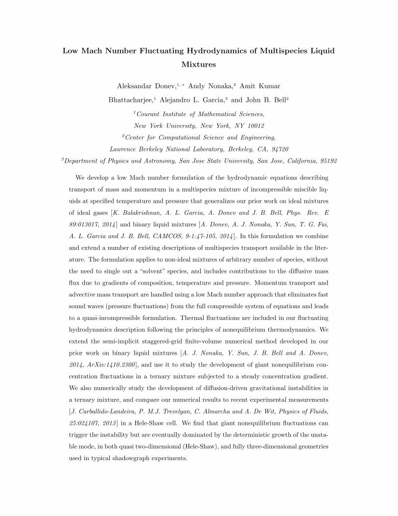
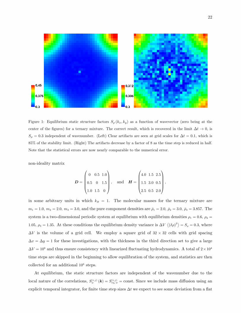
Figure 1: Equilibrium static structure factors Sρ (kx, ky) as a function of wavevector (zero being at the

center of the figures) for a ternary mixture. The correct result, which is recovered in the limit ∆t → 0, is

Sρ = 0.3 independent of wavenumber. (Left) Clear artifacts are seen at grid scales for ∆t = 0.1, which is

85% of the stability limit. (Right) The artifacts decrease by a factor of 8 as the time step is reduced in half.

Note that the statistical errors are now nearly comparable to the numerical error.

non-ideality matrix

D =

0 0.5 1.0

0.5 0 1.5

1.0 1.5 0

, and H =

4.0 1.5 2.5

1.5 3.0 0.5

2.5 0.5 2.0

,

in some arbitrary units in which kB = 1. The molecular masses for the ternary mixture are

m1 = 1.0, m2 = 2.0, m3 = 3.0, and the pure component densities are ρ1 = 2.0, ρ2 = 3.0, ρ3 = 3.857. The

system is a two-dimensional periodic system at equilibrium with equilibrium densities ρ1 = 0.6, ρ2 =

1.05, ρ3 = 1.35. At these conditions the equilibrium density variance is ∆V⟨(δρ)

2⟩

= Sρ = 0.3, where

∆V is the volume of a grid cell. We employ a square grid of 32 × 32 cells with grid spacing

∆x = ∆y = 1 for these investigations, with the thickness in the third direction set to give a large

∆V = 106 and thus ensure consistency with linearized fluctuating hydrodynamics. A total of 2×104

time steps are skipped in the beginning to allow equilibration of the system, and statistics are then

collected for an additional 106 steps.

At equilibrium, the static structure factors are independent of the wavenumber due to the

local nature of the correlations, S(i,j)w (k) = S(i,j)

eq, w = const. Since we include mass diffusion using an

explicit temporal integrator, for finite time step sizes ∆t we expect to see some deviation from a flat

23

0 0.5 1 1.5 2

0.001

0.01

0.1

time

Sw(i,j) (k

,t)

S(1,2)

w(k,t)

S(1,3)

w(k,t)

S(2,3)

w(k,t)

0 0.5 1 1.5

0.01

0.1

0.3

time

Sρ(k

,t)

Sρ(κ

x=0, κ

y=2, t)

Sρ(κ

x=0, κ

y=4, t)

Sρ(κ

x=4, κ

y=4, t)

Sρ(κ

x=2, κ

y=8, t)

Sρ(κ

x=8, κ

y=8, t)

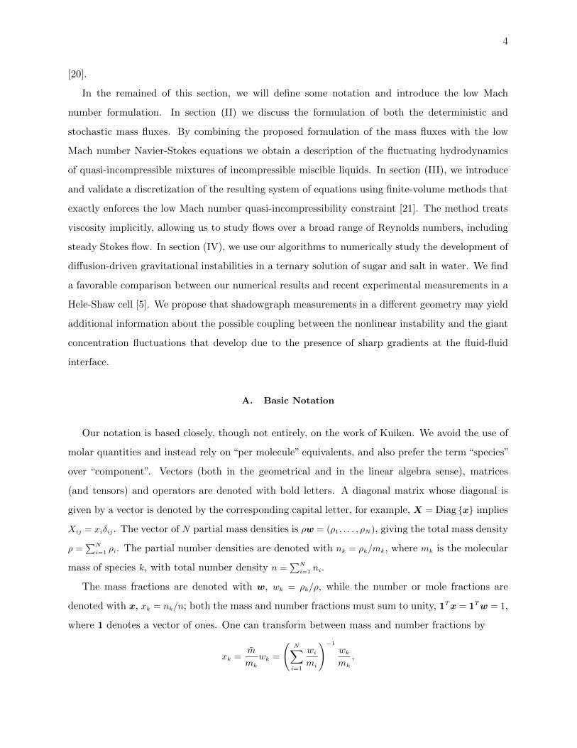
Figure 2: Equilibrium dynamic structure factors Sw (k, t) for a ternary mixture, as a function of time for

wavenumber k = (κx, κy) · 2π/L. Numerical results are shown with symbols and theoretical predictions are

shown with solid lines of the same color as the corresponding symbols. (Left) S(i,j)w (k, t) for κx = κy = 4

for i 6= j. (Right) Sρ (k, t) for several wavenumbers. Note that at large times statistical noise begins to

dominate the signal.

spectrum at the largest wavenumbers (i.e., for k ∼ ∆x−1) [40, 41]. In Fig. 1 we show the spectrum

of density fluctuations at equilibrium for two different time step sizes, a large time step size ∆t = 0.1

(left panel), and a smaller time step size ∆t = 0.05 (right panel). Since the largest eigenvalue of

the diffusion matrix is around χ ≈ 2, the largest stable time step size is ∆tmax ≈ 0.12. As seen in

the figure, for ∆t = 0.1, which is close to the stability limit, we see a significant enlargement of the

fluctuations at the corners of the Fourier grid; when we reduce the time step by a factor of 2 we

reduce the error by a factor of around 8, consistent with the fact that the explicit midpoint method

used in our overdamped algorithm [12] is third-order accurate for static covariances [40]. Therefore,

in the limit of sufficiently small time steps we will recover the correct flat spectrum, demonstrating

that our equations and our numerical scheme obey a fluctuation-dissipation principle.

In the left panel of Fig. 2 we show numerical results for the dynamic structure factors S(i,j)w (k, t)

for several i 6= j for k = (4, 4) ·2π/L, where L = 32 is the length of the square domain. Note that the

factors for i = j are not statistically independent due to the constraint that mass fractions sum to

unity, and are thus not shown. In the right panel of Fig. 2 we show numerical results for Sρ (k, t),

given by (34), for several different wavenumbers k = (κx, κy) · 2π/L. We compare the numerical

results to the theoretical prediction (D3), which is a sum of two exponentially-decaying functions.

Excellent agreement is seen between simulation and theory, demonstrating that our numerical

24

method correctly reproduces both the statics and dynamics of the compositional fluctuations.

2. Non-Equilibrium Fluctuations

Fluctuations in systems out of equilibrium are known to be long-range correlated and signifi-

cantly enhanced compared to equilibrium. In particular, in the presence of an imposed (macro-

scopic) concentration gradient, concentration fluctuations exhibit a characteristic power-law static

structure factor ∼ k−4 [1]. In Section IV.C in Ref. [9], we studied the long-ranged (giant) concen-

tration fluctuations in a ternary mixture in the presence of a gradient imposed via the boundary

conditions, and confirmed that our multispecies compressible algorithm correctly reproduced the-

oretical predictions; here we repeat this test but for a mixture of three incompressible liquids.

In order to simplify the theoretical calculations, see Appendix B in Ref. [9], we take the first

two of the three species to be dynamically identical (indistinguishable), and take the molecular

masses to be equal, m1 = m2 = m3 = 1.0 (this makes mass and mole fractions identical). The

Stefan-Maxwell diffusion matrix is taken to be

D =

0 2.0 1.0

2.0 0 1.0

1.0 1.0 0

and the mixture is assumed to be ideal, H = 0, and isothermal, ∇T = 0. In order to focus our

attention on the nonequilibrium fluctuations we set the stochastic mass flux to zero, F = 0; this

ensures that all concentration fluctuations come from the coupling to the velocity fluctuations via

the gradient and eliminate the statistical errors coming from a finite background spectrum. The

pure component densities are ρ1 = ρ2 = ρ3 = 1.0, giving an incompressible fluid, ∇ ·v = 0, consistent

with the theoretical calculations. A weak concentration gradient is imposed by enforcing Dirichlet

(reservoir [11]) boundary conditions for the mass fractions at the top and bottom boundaries,

w (y = 0, t) = (0.2493, 0.245, 0.5057) and w (y = L, t) = (0.250729, 0.255, 0.494271). These values are

chosen so that the deterministic diffusive flux of the first species vanishes at y = L/2, F1 (y = L/2, t) =

0, leading to a diffusion barrier for the first species, as in Ref. [9].

The computational grid has 128×64 grid cells with grid spacing ∆x = ∆y = 1, with the thickness

in the third direction set to give ∆V = 106, and time step ∆t = 0.1. In order to study the spectrum

of the giant concentration fluctuations, we compute the Fourier spectrum of the mass fractions

averaged along the direction of the gradient; this corresponds to ky = 0 and thus k = kx. A total

of 1.8 × 105 time steps are preformed at the beginning of the simulation to allow the system to

25

0.0625 0.125 0.25 0.5 1 2

10−16

10−15

10−14

10−13

10−12

10−11

10−10

10−9

k

ν ×

Sw(i,j)

ν × Sw

(1,1) no−slip

ν × Sw

(2,2) no−slip

ν × Sw

(1,2) no−slip

0.0625 0.125 0.25 0.5 1 2

10−14

10−13

10−12

10−11

10−10

10−9

k

ν ×

Sw(2

,2)

Simulation, ν=1

Simulation, ν=10

Simulation, ν=100

Simulation, ν=1000

theory, ν=1

theory, ν=10

Overdamped

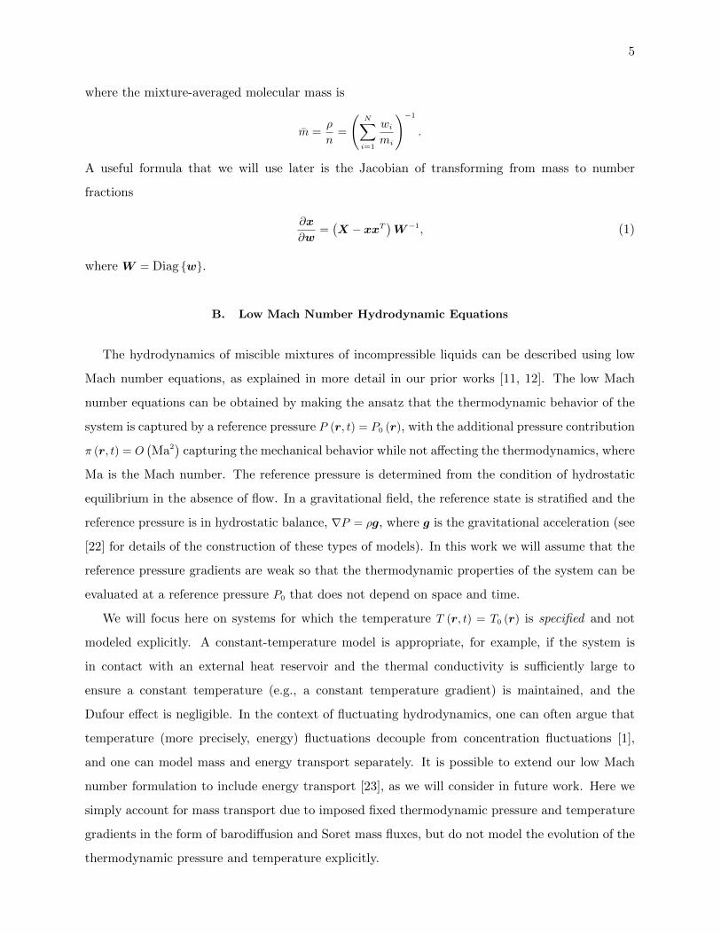
Figure 3: Static structure factors of the mass fractions averaged along the direction of the gradient, exhibiting

giant ∼ k−4 fluctuations. (Left) Cross-correlations for the overdamped equations. Filled symbols are for

no-slip boundary conditions for velocity, while empty ones are for free-slip boundaries. Lines of the same

color show the theoretical prediction in a “bulk” system (no boundaries). (Right) Spectrum of fluctuations

of w2 for several different values of the viscosity for the inertial equations. The overdamped theory is

shown for comparison. For ν = 1 (Schmidt number ∼ 1) a difference between the inertial and overdamped

results is seen and reproduced well by the numerical scheme. For ν & 10 there is very little difference

between overdamped and inertial, and the two algorithms produce similar results. For very large viscosities,

however, one should use the overdamped integrator, as evidenced by the notable departure from the theory

at large wavenumbers for ν = 1000.

equilibrate. Statistics are then collected for 5× 105 steps.

In this nonequilibrium example the coupling to the velocity equation is crucial and is the cause

of the giant fluctuations. The normal component of the velocity at the two physical boundaries

follows from the EOS and the diffusive fluxes through the boundary, see Eq. (15) in Ref. [11].

For the tangential (x) component of velocity we use either no-slip (zero velocity) or free-slip (zero

shear stress) boundary conditions. In the limit of infinite Schmidt number, ν = η/ρ � χ, where χ

is a typical mass diffusion coefficient, the overdamped equations apply and ν S(i,j)w (k) approaches a

limit independent of the actual value of the Schmidt number. For finite Schmidt numbers, however,

the actual value of the Schmidt number affects the spectrum, see Appendix B in Ref. [9] for the

explicit formulas.

For the overdamped integrator, the actual value of the viscosity does not matter beyond sim-

ply rescaling the amplitude of the fluctuations, since the velocity equation is a time-independent

(steady) Stokes equation in the viscous-dominated limit. In the left panel of Fig. 3 we show nu-

26

merical results for ν S(i,j)w (k) for i 6= j, obtained using our overdamped algorithm [12]. Excellent

agreement with the theoretical prediction in Appendix B in Ref. [9] is seen for wavenumbers larger

than L−1; for small wavenumbers the confinement suppresses the giant fluctuations in a manner

that depends on the specific boundary conditions imposed [10]. In the right panel of Fig. 3 we show

ν S(2,2)w (k) for several values of the kinematic viscosity, as obtained using our inertial algorithm [12].

The implicit-midpoint (Crank-Nicolson) scheme used to treat viscosity in the inertial algorithm is

unconditionally stable and allows an arbitrary time step size to be used. It is, however, well-known

that this kind of scheme can produce unphysical results for very large viscous Courant numbers

due to fact it is not L-stable (see discussion in Appendix B in Ref. [40]). This is seen in the results

in the right panel of Fig. 3 for the largest viscosity ν = 1000 (corresponding to viscous Courant

number ν∆t/∆x2 = 100) at the larger wavenumbers. It is actually quite remarkable that we can use

the inertial integrator with rather large time step sizes and get very good results over most of the

wavenumbers of interest; this is a property that stems from a specific fluctuation-dissipation balance

in the implicit midpoint scheme [40]. These results demonstrate that both our overdamped and

inertial methods are able to reproduce the correct spectrum of the nonequilibrium concentration

fluctuations.

3. Thermodiffusion and Barodiffusion

In the giant fluctuation example shown in Fig. 3, the system was kept out of equilibrium by

imposed concentrations on the boundaries, which is difficult to realize in experiments. Instead,

experiments that measure giant fluctuations in liquid mixtures typically rely on the Soret effect

to induce a concentration gradient via an imposed temperature gradient [42]. A concentration

gradient can also be induced via barodiffusion in the presence of large gravitational accelerations,

as used in ultracentrifuges for the purposes of separation of macromolecules and isotopes [14].

Barodiffusion and thermodiffusion enter in the density equations (30) in the same manner, however,

the key difference is that barodiffusion requires gravity which also enters via the buoyancy term

in the velocity equation (3,5). Furthermore, the steady state gradient induced by barodiffusion

is determined by equilibrium thermodynamics only and does not involve any kinetic transport

coefficients.

It is well known that there is no nonequilibrium enhancement of the fluctuations at steady

state for a system in a gravitational field [43] in the absence of external forcing (see Eq. (28) in

27

[44]) 5. This is because the system is still in thermodynamic equilibrium, despite the presence

of spatial nonuniformity (sedimentation). In particular, without doing any calculations we know

that the equilibrium distribution of the fluctuations is the Gibbs-Boltzmann distribution, with a

local free-energy functional that now includes a gravitational energy contribution. In this section

we demonstrate that our low Mach number approach captures this important distinction between

(ordinary) equilibrium fluctuations in the presence of barodiffusion, and (giant) nonequilibrium

fluctuations in the presence of thermodiffusion.

We consider a solution of potasium salt and sucrose in water (see Section IV for more details) in

an ultracentrifuge. The physical parameters of this ternary mixture are given in Section IV A, and

a brief theoretical analysis is given in Appendix B. We perform two dimensional simulations of a

system of physical dimensions 0.8× 0.8× 0.1cm divided into 64× 64× 1 finite-volume cells. Periodic

boundary conditions are used in the x direction and impermeable no-slip boundaries are used in the

y direction. The average mass fractions over the domain are set to wav = (0.0492, 0.0229, 0.9279) . A

total of 0.5 · 106 time steps are performed at the beginning of the simulation to allow the system to

equilibrate before statistics are collected for 106 steps.

In order to induce a strong sedimentation in this mixture we need to increase the ratio m2g/ (kBT )

by six orders of magnitude relative to its reference value on Earth (see (B2)). In actual experiments

this would be accomplished by increasing the effective gravity (i.e., centrifugal acceleration) in an

ultracentrifuge; however, increasing gravity by such a large factor makes the system of equations

(3,5,30) numerically too stiff for our semi-implicit temporal integrator. This is because buoyancy

changes the time scale for relaxation of large-scale (small wavenumber) concentration fluctuations

from the usual slow diffusive relaxation to a very fast non-diffusive relaxation [45]. Therefore,

instead of increasing g we artificially decrease kB by six orders of magnitude, and apply Earth

gravity g = −981 along the negative y direction. With these parameters our inertial temporal

integrator is stable with time step size up to about ∆t = 0.5s; the results reported below are for

∆t = 0.25s.

For comparison, we use the same parameters but turn gravity off and induce a concentration

gradient via thermodiffusion. Specifically, we set the temperature at the bottom wall to 293K

and 300K at the top wall, and set the thermodiffusion constants to the artifical values D(T ) =

(−5 · 10−4,−2 · 10−4, 7 · 10−4). These values ensure that the steady state vertical profiles of the mass

fraction of salt and sugar are very similar between the barodiffusion and thermodiffusion simulations

5 Note, however, that the dynamics of the fluctuations is affected by gravity and by barodiffusion [44]

28

0 0.1 0.2 0.3 0.4 0.5 0.6 0.7 0.8

Height h

0

0.01

0.02

0.03

0.04

0.05

0.06

0.07

0.08

0.09M

ass

frac

tion

Salt (barodiffusion)

Sugar (barodiffusion)

Salt (thermodiffusion)

Salt (barodiffusion)

16 32 64 128Wavenumber k

10-23

10-22

10-21

10-20

10-19

10-18

Spec

trum

S

ρ(k)

UniformBarodiffusionThermodiffusion

k-4

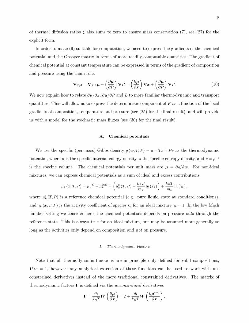
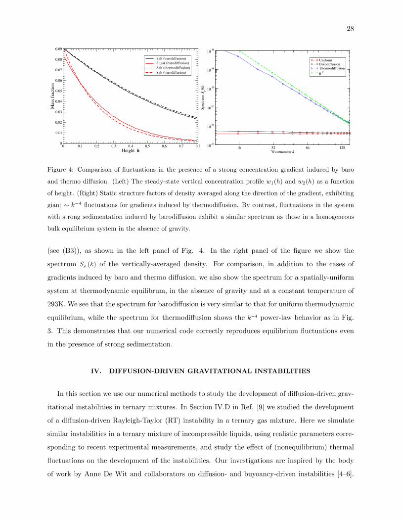
Figure 4: Comparison of fluctuations in the presence of a strong concentration gradient induced by baro

and thermo diffusion. (Left) The steady-state vertical concentration profile w1(h) and w2(h) as a function

of height. (Right) Static structure factors of density averaged along the direction of the gradient, exhibiting

giant ∼ k−4 fluctuations for gradients induced by thermodiffusion. By contrast, fluctuations in the system

with strong sedimentation induced by barodiffusion exhibit a similar spectrum as those in a homogeneous

bulk equilibrium system in the absence of gravity.

(see (B3)), as shown in the left panel of Fig. 4. In the right panel of the figure we show the

spectrum Sρ (k) of the vertically-averaged density. For comparison, in addition to the cases of

gradients induced by baro and thermo diffusion, we also show the spectrum for a spatially-uniform

system at thermodynamic equilibrum, in the absence of gravity and at a constant temperature of

293K. We see that the spectrum for barodiffusion is very similar to that for uniform thermodynamic

equilibrium, while the spectrum for thermodiffusion shows the k−4 power-law behavior as in Fig.

3. This demonstrates that our numerical code correctly reproduces equilibrium fluctuations even

in the presence of strong sedimentation.

IV. DIFFUSION-DRIVEN GRAVITATIONAL INSTABILITIES

In this section we use our numerical methods to study the development of diffusion-driven grav-

itational instabilities in ternary mixtures. In Section IV.D in Ref. [9] we studied the development

of a diffusion-driven Rayleigh-Taylor (RT) instability in a ternary gas mixture. Here we simulate

similar instabilities in a ternary mixture of incompressible liquids, using realistic parameters corre-

sponding to recent experimental measurements, and study the effect of (nonequilibrium) thermal

fluctuations on the development of the instabilities. Our investigations are inspired by the body

of work by Anne De Wit and collaborators on diffusion- and buyoancy-driven instabilities [4–6].

29

In particular, in Ref. [5] a classification of these instabilities in a ternary mixture are proposed,

and several of the instabilities are investigated experimentally. In the first part of this section

we perform simulations of the experimental measurements of a mixed-mode instability (MMI). In

the second part we investigate diffusive layer convection (DLC) (just as we did in Section IV.D in

Ref. [9] for gases), in a hypothetical shadowgraphy or light scattering experiment that could, in

principle, be performed in the laboratory.

We begin with a brief summary of the experimental setup of Carballido-Landeira et al. [5]

for getting a diffusion-driven gravitational instability in a simple ternary mixture: a solution of

salt in water on top of a solution of sugar in water. The concentrations of salt and sugar are

small so that even though this is a ternary mixture in this very dilute limit one can think of salt

and sugar diffusing in water without significant interaction. The key here is the difference in the

diffusion coefficient between sugar (a larger organic molecule diffusing slower) and salt (a smaller

ion diffusing faster) in water. Both sugar and salt solutions have a density that grows with the

concentration of the solute.

In the experiments, one starts with an almost (to within experimental controls) flat and almost

sharp interface between the two solutions. Even if one starts in a stable configuration, with the

denser solution on the bottom, the differential diffusion effects can create a local minimum in

density below the contact line and a local maximum above the contact line. This leads to an

unstable configuration and the development of DLC at symmetric distances above and below the

contact line. If one starts with an unstable configuration of the denser solution on top, before the

RT instability has time to develop and perturb the interface, differential diffusion effects can lead to

the development of local extrema in the density above and below the contact line that are outside

the range of the initial densities. The dynamics is then a combination of RT and DLC giving

rise to a mixed mode instability (MMI). The DLC leads to characteristic “Y shaped” convective

structures developing around the interface at the locations of the local adverse density gradients,

which evolve around an interface that is slowly perturbed by the RT growth to a finite amplitude

modulation. See Section III in Ref. [5] for more details, and the bottom row of panels in Fig. 1

in Ref. [5], as well as our numerical results in Fig. 6, for an illustration of the development of the

instability.

30

A. Physical Parameters

We use CGS units in what follows (centimeters for length, seconds for time, grams for mass).

Following the experiments of Carballido-Landeira et al., we consider a ternary mixture of potassium

salt (KCl, species 1, molar mass M1 = 74.55, denoted by A in [5]), sugar (sucrose, species 2, molar

mass M2 = 342.3, denoted by B in [5]) and water (species 3, molar mass M3 = 18.02), giving molecular

masses m = (1.238 · 10−22, 5.684 · 10−22, 2.99 · 10−23). The initial configuration is salt solution on top

of sugar solution. In Ref. [5], it is assumed that the density dependence on the concentration can

be captured by (this is a good approximation for very dilute solutions)

ρ = ρ0 (1 + α1Z1 + α2Z2) = ρ0

(1 +

α1

M1

ρ1 +α2

M2

ρ2

), (36)

where ρ0 = ρ3 = 1.0 is the density of water, α1 = 48 for KCl and α2 = 122 for sucrose, and Zk is the

molar density of each component, related to the partial density via ρk = ZkMk, where Mk is the

molar mass. Noting that we can write our EOS (2) in the form

ρ1ρ1

+ρ2ρ2

+ρ− ρ1 − ρ2

ρ3= 1, (37)

and comparing (37) and (36), we get

1− ρ0ρk

= ρ0αkMk

,

which gives us the EOS parameters

ρ1 = 2.81 and ρ2 = 1.55.

Note that here these should not be thought of as pure component densities since the solubility

of the solvents in water is finite, rather, they are simply parameters that enable us to match our

model EOS (2) to the empirical density dependence in the dilute regime.

For the dilute solutions we consider here it is sufficient to assume that D is constant for the

range of compositions of interest, and the mixtures are essentially ideal, H = 0. We also assume

isothermal conditions with the ambient temperature to T = 293K, and assume constant viscosity

η = 0.01. Since the ternary mixture under consideration is what can be considered“infinite dilution”,

we rely on the approximation proposed in Ref. [27],

D13 = D1, D23 = D2, D12 =D1D2

D3

,

where from table I in Ref. [5] we read the diffusion coefficient of low-dilution KCl in water as

D1 = 1.91 · 10−5, and the diffusion coefficient of dilute sucrose in water as D2 = 0.52 · 10−5. Here D3

is the self-diffusion coefficient of pure water, D3 = 2.3 · 10−5, giving D12 ≈ 4.32 · 10−6.

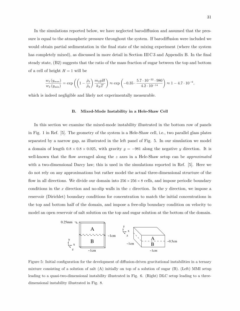
31

In the simulations reported below, we have neglected barodiffusion and assumed that the pres-

sure is equal to the atmospheric pressure throughout the system. If barodiffusion were included we

would obtain partial sedimentation in the final state of the mixing experiment (where the system

has completely mixed), as discussed in more detail in Section III C 3 and Appendix B. In the final

steady state, (B2) suggests that the ratio of the mass fraction of sugar between the top and bottom

of a cell of height H = 1 will be

w2 (ymax)

w2 (ymin)= exp

((1− ρ3

ρ2

)m2gH

kBT

)≈ exp

(−0.35 · 5.7 · 10−22 · 980

4.2 · 10−14

)≈ 1− 4.7 · 10−6,

which is indeed negligible and likely not experimentally measurable.

B. Mixed-Mode Instability in a Hele-Shaw Cell

In this section we examine the mixed-mode instability illustrated in the bottom row of panels

in Fig. 1 in Ref. [5]. The geometry of the system is a Hele-Shaw cell, i.e., two parallel glass plates

separated by a narrow gap, as illustrated in the left panel of Fig. 5. In our simulation we model

a domain of length 0.8 × 0.8 × 0.025, with gravity g = −981 along the negative y direction. It is

well-known that the flow averaged along the z axes in a Hele-Shaw setup can be approximated

with a two-dimensional Darcy law; this is used in the simulations reported in Ref. [5]. Here we

do not rely on any approximations but rather model the actual three-dimensional structure of the

flow in all directions. We divide our domain into 256× 256× 8 cells, and impose periodic boundary

conditions in the x direction and no-slip walls in the z direction. In the y direction, we impose a

reservoir (Dirichlet) boundary conditions for concentration to match the initial concentrations in

the top and bottom half of the domain, and impose a free-slip boundary condition on velocity to

model an open reservoir of salt solution on the top and sugar solution at the bottom of the domain.

B

A

~1cm

~1cm

z

x

y

0.25mm

A

B

~1cm

~1cm~0.5cm

z

x

y

Figure 5: Initial configuration for the development of diffusion-driven gravitational instabilities in a ternary

mixture consisting of a solution of salt (A) initially on top of a solution of sugar (B). (Left) MMI setup

leading to a quasi-two-dimensional instability illustrated in Fig. 6. (Right) DLC setup leading to a three-

dimensional instability illustrated in Fig. 8.

32

Note that the momentum diffusion time across a domain of length L ∼ 1 is τL ∼ L2/(2ν) ≈ 50. The

experimental snapshots in Fig. 1 of Ref. [5] indicate that this is comparable to the time it takes for

the instability to fully develop. It is therefore not safe to rely on the overdamped approximation, so

we use the inertial integrator described in Ref. [12] in our simulations. Nevertheless the overdamped

limit is a relatively good approximation in practice since the characteristic length scale of the Y -

shaped DLC fingers observed in the experiments is L ∼ 0.013, corresponding to viscous diffusion

time τL ∼ 8.5 · 10−3. We have compared numerical simulations using the overdamped and inertial

integrators and found little difference. We simulate the development of the instability to t ≈ 63.9

with a fixed time step size of ∆t = 6.39 · 10−2, which corresponds to 75% of the stability limit

dictated by our explicit treatment of mass diffusion. We use a centered discretization of advection;

in these well-resolved simulations little difference is observed between centered advection and the

more sophisticated BDS advection scheme [34] summarized in Ref. [12].

The initial concentrations, denoted with superscript zero in what follows, on the top and bottom

are determined from the dimensionless ratio reported in [5],

R =α2Z

02

α1Z01

=α2w2/M2

α1w1/M1

= 0.89. (38)

Specifically, we set the initial mass fractions of salt and sugar to w01 = 0.0864 and w0

2 = 0.1368

respectively, more precisely,

w0top = (0.0864, 0, 0.9136)

w0bottom = (0, 0.1368, 0.8632)

which, from the EOS (2) gives a density difference of about 0.8%. Similar results are observed

for other values of the concentrations if the dimensionless ratio R in (38) is kept fixed, with the

main difference being that lower concentrations lead to a slower development and growth of the

instability.

In the experiments, the initial interface between the two solutions is not, of course, perfectly flat.

To model this effect, it is common in the literature to add a small random perturbation to the initial

conditions. Assuming that the growth of the unstable modes is exponential in time, the time it will

take for the instability to reach a certain point in its development (e.g., to first split the Y-shaped

fingers) will depend on the amplitude of the initial perturbation. Since the initial condition is not

known to us and is impossible to measure experimentally to high accuracy, it is not possible to

directly compare snapshots of the instability at “the same point in time” between simulations and

experiments, or between simulations that use different initial perturbations. Instead, we compare a

33

Figure 6: Development and growth of a mixed-mode instability in a Hele-Shaw setup. Two-dimensional

slices of the three-dimensional density field are shown as color plots at times t ≈ 13 (top row), t ≈ 26

(middle row) and t ≈ 51 (bottom row). The square images show ρ (x, y, z = 0.0125) (halfway between the

glass plates) and the thin vertical images show the corresponding slice ρ (x = 0, y, z) (corresponding to the

left edge of the square images). Compare these to the experimental results shown in the bottom row of

panels in Fig. 1 in Ref. [5]. (Left) With random initial perturbation and thermal fluctuations. (Right)

Deterministic simulation starting with the same random initial perturbation as for the left panels, but no

thermal fluctuations.

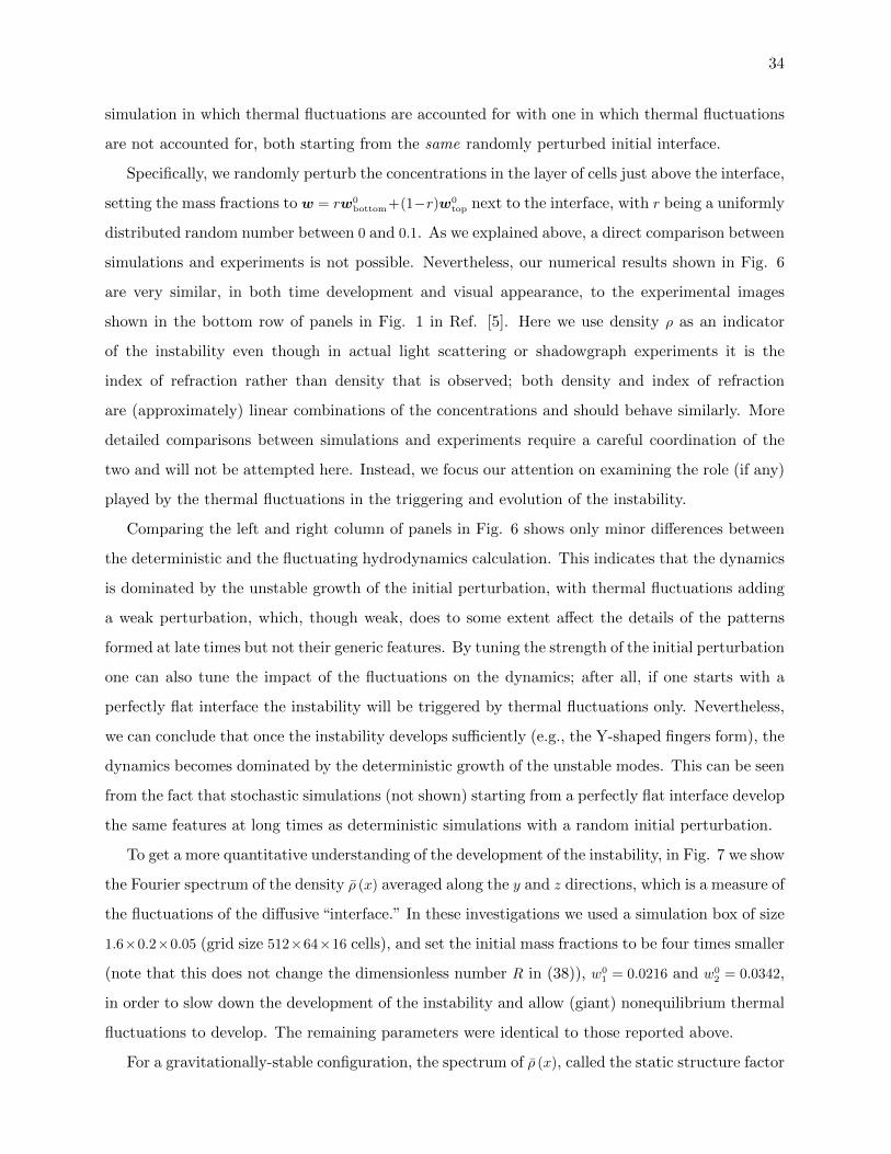
34

simulation in which thermal fluctuations are accounted for with one in which thermal fluctuations

are not accounted for, both starting from the same randomly perturbed initial interface.

Specifically, we randomly perturb the concentrations in the layer of cells just above the interface,

setting the mass fractions to w = rw0bottom+(1−r)w0

top next to the interface, with r being a uniformly

distributed random number between 0 and 0.1. As we explained above, a direct comparison between

simulations and experiments is not possible. Nevertheless, our numerical results shown in Fig. 6

are very similar, in both time development and visual appearance, to the experimental images

shown in the bottom row of panels in Fig. 1 in Ref. [5]. Here we use density ρ as an indicator

of the instability even though in actual light scattering or shadowgraph experiments it is the

index of refraction rather than density that is observed; both density and index of refraction

are (approximately) linear combinations of the concentrations and should behave similarly. More

detailed comparisons between simulations and experiments require a careful coordination of the

two and will not be attempted here. Instead, we focus our attention on examining the role (if any)

played by the thermal fluctuations in the triggering and evolution of the instability.

Comparing the left and right column of panels in Fig. 6 shows only minor differences between

the deterministic and the fluctuating hydrodynamics calculation. This indicates that the dynamics

is dominated by the unstable growth of the initial perturbation, with thermal fluctuations adding

a weak perturbation, which, though weak, does to some extent affect the details of the patterns

formed at late times but not their generic features. By tuning the strength of the initial perturbation

one can also tune the impact of the fluctuations on the dynamics; after all, if one starts with a

perfectly flat interface the instability will be triggered by thermal fluctuations only. Nevertheless,

we can conclude that once the instability develops sufficiently (e.g., the Y-shaped fingers form), the

dynamics becomes dominated by the deterministic growth of the unstable modes. This can be seen

from the fact that stochastic simulations (not shown) starting from a perfectly flat interface develop

the same features at long times as deterministic simulations with a random initial perturbation.

To get a more quantitative understanding of the development of the instability, in Fig. 7 we show

the Fourier spectrum of the density ρ (x) averaged along the y and z directions, which is a measure of

the fluctuations of the diffusive “interface.” In these investigations we used a simulation box of size

1.6×0.2×0.05 (grid size 512×64×16 cells), and set the initial mass fractions to be four times smaller

(note that this does not change the dimensionless number R in (38)), w01 = 0.0216 and w0

2 = 0.0342,

in order to slow down the development of the instability and allow (giant) nonequilibrium thermal

fluctuations to develop. The remaining parameters were identical to those reported above.

For a gravitationally-stable configuration, the spectrum of ρ (x), called the static structure factor

35

8 16 32 64 128 256 512 1024

Wavenumber k (cm-1)

10-20

10-18

10-16

10-14

10-12

10-10

Sp

ectr

um

S

(k)

Initial perturbation

No fluct t~13sNo fluct t~26sNo fluct t~51sWith fluct t~13sWith fluct t~26sWith fluct t~51sg=0, t=64s

k-4

Figure 7: Early time development of a mixed-mode instability instability in a Hele-Shaw cell. The spectrum

S(k) of the density averaged along the vertical direction and the thickness of the sample is shown as a

function of wavenumber, at several points in time. The same random initial perturbation is added to the

initial condition (black solid line) in all simulations. A first simulation is deterministic, and clearly shows an

unstable (exponential) growth for modes with k . 64, while larger wavenumbers decay in time. A second

simulation accounts for nonequilibrium thermal fluctuations, and displays giant fluctuations in addition to

the unstable growth. At late times nonlinearities trigger all modes to show a nontrivial spectrum, not affected

significantly by the thermal fluctuations. Note that the most unstable (growing) mode has wavelength of

about 1.4mm which compares very favorably to the experimentally-reported 1.3mm [5]. A third simulation

is in microgravity (g = 0) and shows a slow development of a stable k−4 giant fluctuation spectrum.

S(k), exhibits a characteristic giant fluctuation k−4 power-law decay at large wavenumbers k at long

times [1], as illustrated in Fig. 3 by showing S(k) for a simulation in which gravity is switched off.

At small wavenumbers, gravity and confinement damp the amplitude and affect the dynamics of the

giant fluctuations, as is well-understood for stable steady states [1, 10, 44–46]. We emphasize that

the thermal fluctuations in these investigations are completely dominated by the nonequilibrium

(giant) fluctuations induced by the presence of large concentration gradients at the interface; the

equilibrium concentration fluctuations are many orders of magnitude weaker in comparison. This

is seen by the fact that we observe identical results if we completely turn off the stochastic mass

fluxes, and keep only the stochastic momentum flux (velocity fluctuations). Similarly, turning off

the stochastic momentum flux but keeping the stochastic mass flux, in this particular setup, leads

36

to very small fluctuations that are below the tolerance of our linear solvers.

To our knowledge, nonequilibrium fluctuations have not been examined in an unstable situation

like the one we study here; some studies have been carried out near the onset of the Rayleigh-

Bernard thermal convection instability [47, 48]. It is important to emphasize that the very validity

of fluctuating hydrodynamics has not been established for unstable flows; one can justify linearized

fluctuating hydrodynamics [1, 49, 50], but in a linearization the fluctuations do not affect the

deterministic flow and thus cannot trigger the instability. The results in Fig. 7 show that in the

absence of thermal fluctuations, there is a clear band of wavenumbers k . 64 whose amplitude grows

in time due to the instability, while the remaining modes decay to zero rapidly. It is important to

note that the most unstable wavelength of λ ≈ 2π/45 ≈ 0.14cm is very close to the experimentally

reported value of 0.13cm [5]. When thermal fluctuations are present, the same band of wavenumbers

grows in a similar manner, but at the same time, larger wavenumbers show a nontrivial power-

law spectrum. Eventually, however, the unstable modes completely dominate the dynamics and

there is essentially no difference between the simulations with and without thermal fluctuations;

to make a more precise quantitative statement multiple Monte Carlo simulations are required to

perform ensemble averages and reduce the statistical error, as well as to eliminate the effects of

the boundary conditions along the horizontal and vertical directions. Note that at later times the

fluid flow becomes chaotic and further information may be gained by also examining the spectrum

of the fluid velocity and not just the vertical projection of the density; we leave such detailed

investigations for future studies.

C. Diffusive-Layer Convection (DLC) instability

In this section we use our algorithm to model a hypothetical experiment in which the gravity

points in the direction perpendicular to the fluid-fluid interface and do the confining glass slips,

as illustrated in the right panel of Fig. 5. This kind of geometry has already been used to

experimentally investigate isothermal free diffusive mixing in a binary liquid mixture [45] in a

stable configuration 6. To our knowledge, similar experiments have not been performed for ternary

mixtures, although it is feasible they could be if the initial configuration can be prepared with

sufficient control.

To be specific, we select the initial concentrations of the sugar and salt solutions to get a

6 Note that for a binary mixture the only alternative to a stable configuration is to have an RT-unstable configuration.

37

diffusive layer convection (DLC) instability; all other parameters are the same as for the MMI

setup summarized above. The dimensionless parameter used for Fig. 1(c) in Ref. [5] is

R =α2Z

02

α1Z01

= 1.25,

giving the required ratio of mass fractions,

w01

w02

=α1Z

01

α2Z02

· α2M1

α1M2

=1

R· α2M1

α1M2

= 0.44.

We set w01 = 0.022 and w0

2 = 0.05, which gives an initial density of 1.014375 on the top and 1.018062

on the bottom, for a density difference of about -0.4% (recall that the sign of the difference is

opposite for DLC and MMI configurations).

The dimensions of the domain in our simulations are 1 × 0.5 × 1, with periodic boundary con-

ditions in x and z, and reservoir (Dirichlet) boundary condition for concentration together with

free-slip boundary condition on velocity in the y direction. The grid is 256 × 128 × 256 grid cells,

and the time step size is fixed at ∆t = 0.025, which corresponds to a maximum advective Courant

number of ∼ 0.5. We treat advection using the unlimited bilinear BDS high-resolution scheme [51]

summarized in Ref. [12]. The initial interface is now perfectly flat, so that the instability is triggered

by the nonequilibrium (giant) thermal fluctuations. We focus our investigation here on the differ-

ences in the spectrum of the thermal fluctuations with (unstable) and without (marginally stable)

gravity. Note that experimental measurements of giant concentration fluctuations in microgravity

are feasible and have been performed for binary liquid mixtures [8]; microgravity measurements on

ternary mixtures are ongoing or in the planning stage [3].

In this geometry, the interface between the two fluids cannot be visualized, rather, one sees the

average index of refraction (a linear combination of the average concentrations) along the thickness

of the sample (direction of the gradient and of gravity). In Fig. 8 we show color plots for the

vertically-averaged density at two points in time, one as the instability is just beginning to dominate

the dynamics, and the other as the instability has fully developed. In the presence of gravity, at

early times there are pronounced giant thermal fluctuations in addition to the fluctuations coming

from the growth of the unstable modes, which dominate the dynamics at late times similarly to

the MMI case in Fig. 6. The giant nonequilibrium fluctuations are more clearly visualized by

considering stable free diffusive mixing in microgravity (g = 0, bottom panels).

In Fig. 9, we show the radially-averaged power spectrum S(k = ‖k‖) corresponding to the

vertically-averaged density ρ (x, z). Behavior similar to the MMI instability shown in Fig. 6 is

observed. The band of wavenumbers between 16 . k . 128 is seen to grow in time, and the

38

characteristic k−4 giant fluctuation spectrum is seen at large wavenumbers, especially clear in the

results for microgravity. Deterministic simulations (not shown) starting from a randomly-perturbed

interface show similar unstable growth and are eventually indistinguishable from simulations in

which the instability is triggered and enhanced by thermal fluctuations.

We defer detailed studies of these phenomena for future work, in the hope that our work

will stimulate careful experimental investigations that can directly be compared to our computer

simulations. By adjusting the initial concentrations and the choice of the two solutes one can change

the range of unstable wavenumbers and the time scale for the development of the instability; this

is best done by performing a linear stability analysis [4]. It is feasible that for some choice of

parameters a more substantial interaction between the spectrum at large wavenumbers, dominated

by giant fluctuations, and the spectrum at small wavenumbers, dominated by the instability, will

Figure 8: Development of a fully three-dimensional diffusive layer convection (DLC) instability as a layer

of less-dense salty water is placed on top of a horizontal layer of denser sweet water. The color plots

show the vertically averaged density ρ (horizontal planes) and planar slices of ρ (vertical planes). The

left panels correspond to time t = 15 since the initial contact between the miscible liquids, and the right

panels correspond to t = 19. The top row of panels is for a flat initial interface driven unstable by thermal

fluctuations in the presence of gravity, and the bottom row is in microgravity (g = 0).

39

16 32 64 128 256 512

Wavenumber k (cm-1)

10-20

10-19

10-18

10-17

10-16

10-15

10-14

Sp

ectr

um

S

(k)

g=0, t=15s

g=0, t=19s

g>0, t=15s

g>0, t=19s

k-4

Figure 9: Radially averaged spectrum S(k) of the vertically-averaged density shown in the four panels in

Fig. 8. In Earth gravity (g > 0), the most unstable (growing) mode is seen to have a wavelength of about

2π/32 ≈ 0.2cm, but there is in fact a rather broad range of wavenumbers that are unstable. In microgravity

(g = 0) the deterministic state is stable but the fluctuations grow to be “giant” with a characteristic k−4

power spectrum.

occur. If this is the case one may be able to observe a measurable influence of nonequilibrium

concentration fluctuations on the development and grown of the instability, allowing us, for the first

time, to experimentally access the validity of nonequilibrium nonlinear fluctuating hydrodynamics.

V. CONCLUSIONS

We have developed a low Mach number fluctuating hydrodynamics formulation of momentum

and mass transport in non-ideal mixtures of incompressible liquids with given pure-component

densities. In the present low Mach number model energy transport is not modeled explicitly and

the temperature is assumed constant in time. Momentum transport is accounted for in a quasi-

incompressible framework in which pressure is in mechanical (hydrostatic) equilibrium and fast

sound waves are eliminated from the system of equations because density instantaneously follows

the local composition. The thermodynamics of the mixture is described by the Hessian of the

normalized excess Gibbs energy per particle. The transport properties are given by the shear

viscosity, the Maxwell-Stefan diffusion coefficients, and the thermal diffusion coefficients or ratios,

as a function of the composition of the mixture.

We used our low Mach number algorithm to study the development of gravitational instabilities

during diffusive mixing in ternary mixtures. These mixed mode and diffusive convection instabilities

are specific to mixtures of more than two species and occur because of an interaction between

40

the familiar buoyancy-driven Rayleigh-Taylor instability with differential diffusion effects. Our

simulations of the mixed-mode instability closely mimic recent experiments [5] performed in a Hele-

Shaw setup, and we found good qualitative agreement between experimental and computational

results. A more quantitative comparison is not possible at this stage and should be the subject of

future work. A particularly challenging aspect is to experimentally control or measure the initial

conditions with sufficient accuracy to be able to directly compare simulations to experiments.

Because of the presence of sharp gradients at the interface between the two diffusively mixing

solutions, giant concentration fluctuations develop in the form of power-law tails in the spectrum

of the concentration fluctuations. These nonequilibrium fluctuations are much larger than equilib-

rium ones and have the potential to trigger and feed the instability and affect the growth of the

unstable structures. It is important to observe that such a coupling of the fluctuations back to the

macroscopic dynamics requires nonlinearity, and is not possible in linearized fluctuating hydrody-

namics. While some nonlinear effects in fluctuating hydrodynamics have been verified to occur in

real liquids, it is not clear whether our nonlinear fluctuating hydrodynamic simulations can account

for the effect of the fluctuations on the evolution of the mean flow. In particular, the nonlinear

fluctuating hydrodynamic equations are ill-posed and some regularization, implicit in our finite-

volume discretization, is required to even give meaning to the equations [52]. The conclusions of

the simulations performed here is that fluctuations, despite being “giant”, are quickly overwhelmed

by the deterministic growth of the unstable modes. This suggests that in actual experiments the

development of the instability is primarily triggered by the imperfections in the initial condition

or external fluctuations (e.g., vibrations).

In the Hele-Shaw geometry studied experimentally in [5], the no-slip boundaries strongly damp

the velocity fluctuations and reduce the giant fluctuations. Furthermore, the quasi-two dimensional

geometry limits the possibilities for interactions between the fluctuations and the instability. For

this reason, we also reported simulations of diffusive layer convection for a three-dimensional ge-

ometry, as used in existing experiments in binary mixtures. Because giant fluctuations develop on

a slow diffusive time scale for large and intermediate wavenumbers, it takes some time after the

initial contact between the two fluids for the power-law spectrum to develop. At the same time, the

unstable smaller wavenumbers have an exponentially-growing amplitude, so that the instability can

develop much faster than the giant fluctuations. In our simulations we reduced the concentrations

of solutes to make the density difference very small and thus slow down the unstable growth; it

remains to be seen what is possible and can be observed experimentally.

An important challenge for experimental physicists is to devise ways to measure the thermophys-

41

ical properties in multispecies mixtures [3]. While our formulation can handle mixtures of arbitrary

numbers of species with essentially complete physical fidelity, it is not possible to use our codes for

realistic non-dilute mixtures because many of the parameters, notably the thermodynamic factors

and the Maxwell-Stefan diffusion coefficients, are missing. We believe that it will be necessary to

use computer simulations using the types of methods described here, together with Monte Carlo

sampling of parameters, and potentially also molecular dynamics calculations [37, 53], in addi-

tion to experimental measurement of observation functions, in order to obtain robust estimates of

thermophysical parameters with a quantified uncertainty. The traditional approach of tabulating

values with error bars, that has worked for binary mixtures, fails for multispecies mixtures due to

proliferation of a larger number of parameters that are not all independent but are constrained by

thermodynamic symmetries and stability conditions.

In future work, we will consider the inclusion of chemical reactions in our low Mach number

models. It is also possible to include thermal effects in our formulation by accounting for the

effects of thermal expansion in the quasi-incompressibility constraint. Two key difficulties are

constructing a spatial discretization that ensures preservation of an appropriately generalized EOS,

as well as developing suitable temporal integrators that can handle the multitude of time scales

that appear due the presence of slow mass, fast momentum, and intermediate energy diffusion, and,

potentially, ultrafast chemical reactions. Another challenge for future work on low Mach number

fluctuating hydrodynamics is to account for the effects of surface tension in mixtures of immiscible

or partially miscible liquids. While some thermodynamically-consistent constructions of diffuse-

interface models exist for ternary mixtures [24], we believe that much more work is required to

formulate a complete multispecies system of equations in the presence of square-gradient terms in

the free energy functional, even in the isothermal setting.

Acknowledgments

We would like to thank Anne De Wit and Jorge Carballido Landeira for numerous discussions re-

garding their experiments on gravitational instabilities in ternary mixtures. This material is based

upon work supported by the U.S. Department of Energy Office of Science, Office of Advanced Sci-

entific Computing Research, Applied Mathematics program under Award Number DE-SC0008271

and under contract No. DE-AC02-05CH11231.

42

APPENDIX

Appendix A: COMPUTING THE DIFFUSION MATRIX

An essential complication with treating all species equally, is that the N mass or mole fractions

are not all independent but must sum to unity. For example, the equations (23) are not independent,

and one must supplement them with the condition that the total mass flux is zero. Similarly, the

rows and columns of Λ sum to zero, Λ1 = 0 where 1 denotes a vector of ones, and therefore Λ is

not invertible; the range of Λ are vectors that sum to zero. To deal with these complications, let

us now introduce the projection matrix [18]

Q = I − 1wT ,

which satisfies QTw = Q1 = 0; therefore, pre-multiplying a matrix by QT ensures that the matrix

has a range consisting of vectors that sum to zero, and post-multiplying by QT ensures that the

matrix has w in its null-space. Now, let us define a diffusion matrix as

χ = Q[Λ + αwwT

]−1QT , (A1)

where α 6= 0 is an arbitrary constant, for example, α = Trace (Λ); an alternative equivalent formula

is (24).

Here is a quick summary of some useful relations derived in [54]:

1. Λ1 = 0 and Λ is symmetric positive (semi)definite (SPD) on w⊥.

2. χw = 0 and χ is SPD on 1⊥.

3. χ and Λ are generalized inverses of each other, χΛχ = χ and ΛχΛ = Λ, more specifically,

Λχ = QT and χΛ = Q.

4. The SPD matrices

Λ = Λ + αwwT = χ−1 =(χ+ α−111T

)−1

are inverses of each other, and Λ ≡ Λ on the subspace 1⊥ and χ = χ on the subspace w⊥.

In order to numerically compute χ from Λ, one could use a matrix inverse, as in (24). This fails,

however, when some of the species vanish since the matrix Λ + αwwT is not invertible; this can

be fixed by using a pseudoinverse, computed via the singular value decomposition (SVD) of Λ.

43

However, both matrix inversion and SVD involve O(N3) operations and can be expensive for large

numbers of species. An alternative is to use an iterative numerical procedure [54]

χ = limM→∞

χM = limM→∞

[M∑j=0

(QN)j

]QM−1QT , (A2)

where N = I −M−1Λ, and M is a diagonal matrix with entries

Mii =xi

1− wi

N∑j 6=i=1

xjDij

.

The sum converges rapidly so only a few terms in the sum are needed to compute χM without having

to do matrix inverses, but the speed of convergence is hard to access a priori and in practice we

set M to a fixed integer such as M = 5 or M = 10. It is important to note that, as proven in

[18], the truncated sum to M terms gives an approximation χM ≈ χ that is symmetric positive

semi-definite, and satisfies the properties χMw = 0 as it must. It is therefore perfectly consistent

with thermodynamics to just approximate χ with χM . After all, since the Maxwell-Stefan diffusion

coefficients are only known to at most two decimal places in practice, it makes little sense to invert

Λ exactly or compute its (expensive) SVD. Instead, χM for small M is in practice an equally good

approximation to the true diffusion matrix.

Appendix B: STATIC EQUILIBRIUM OF A DILUTE SOLUTION IN GRAVITY

Barodiffusion is often neglected for liquid mixtures since its contribution to the diffusive fluxes

is typically negligible compared to those due to compositional or temperature gradients, unless

there are very large pressure gradients due to large accelerations, as in ultracentrifuges. Never-

theless, including barodiffusion is crucial in order to obtain the correct equilibrium steady state of

a mixture in the presence of gravity. This is a direct consequence of the fact that barodiffusion

has thermodynamic origin. If barodiffusion is neglected, at thermodynamic equilibrium the mix-

ture would mix uniformly even in the presence of gravity, reaching the state of maximal entropy.

However, physically, we know that heavier species will migrate toward the bottom, minimizing the

free energy by balancing the gain in potential energy with the loss of entropy. Here we show that

once barodiffusion is accounted for the hydrodynamic equations correctly reproduce the statistical

mechanics of systems in a gravitational field.

As a simple case in which we know the “correct” answer, let us focus on the case when the

mixture is a dilute suspension of a number of solutes such as colloids or a macromolecule (e.g.,

solution of sugar in water). In the dilute limit, the different solutes do not affect each other, and

44

we can, in fact, focus on one of the solutes only and consider a binary solution. Let us take the

first species to be the solute and the second species to be the solvent. For a dilute solution, w1 � 1,

Γ ≈ I, m ≈ m2, ρ ≈ ρ2 ≈ ρ2, giving x1 ≈ (m2/m1)w1 and φ1 = wρ/ρ1 ≈ wρ2/ρ1. Note that hydrostatic

equilibrium is built into the low Mach number equations through the reference pressure, which

satisfies dP/dh = ρg, where h is the height. Thermodynamic equilibrium, i.e., a vanishing of the

chemical potential gradients, corresponds to a vanishing of the diffusion driving force for the solute,

d1 =dx1

dh+

(φ1 − w1)

nkBT

dP

dh= 0 ≈ m2

m1

dw1

dh+m2g

kBT

(ρ2ρ1− 1

)w1, (B1)

which directly gives the gravitational sedimentation profile of an ideal gas with molecular mass me,

w1 = w01 exp

(megh

kBT

), (B2)

where me is the excess mass of the colloids over that of the fluid,

me = (ρ1 − ρ2)m1

ρ1=

(1− ρ2

ρ1

)m1.

The result (B2) is in agreement with the statistical-mechanical notion that the solute subsystem

can be thought of as an ideal gas of particles subject to the Archimedean gravity force meg.

A similar calculation for the case of thermodiffusion gives

w1 = w01 exp

(−D

(T )1 −D(T )

2

D12

∇T

Th

), (B3)

which is similar in form but does not have an origin in equilibrium statistical mechanics.

Appendix C: FLUCTUATING MAXWELL-STEFAN DESCRIPTION

In this Appendix, we show that thermal fluctuations can be directly added to the Maxwell-

Stefan formulation in a manner that is intuitive and consistent with the one we presented here,

derived from the principles of nonequilibrium thermodynamics.

In the Maxwell-Stefan description of diffusion, one considers a frictional force between species i

and j proportional to the difference in the particular velocities of the two species, with friction co-

efficient γij = xixj/Dij. It is natural to include thermal fluctuations in this description by including

a fluctuating component to the frictional force with covariance proportional to γij, following the

traditional Langevin approach. This leads us to the MS equation with fluctuations,

di =

N∑j 6=i=1

[γij (vi − vj) +

(2

nγij

) 12

Zij

], (C1)

45

where Zij (r, t) = −Zji (r, t) are space-time white-noise processes, one process per pair of species,

for a total of N (N − 1) /2 random forces. From the above we may augment (20) to account for

fluctuations as

d = −ρ−1ΛW−1F − ∇T

Tζ +

√2

nK Z,

where Z is a vector of N (N − 1) /2 independent white noise processes and K is a matrix that can

directly be read from (C1). Following the same linear algebra steps as before, we can solve for the

fluxes to obtain the additional fluctuating contribution

F = −√

2

nρWχK Z.

The covariance of this stochastic flux is

⟨F (r, t) F (r′, t′)

⟩= 2mρ (Wχ (KK?)χW ) δ (r − r′) δ (t− t′) .

It can be shown that χ (KK?)χ = χ, which shows that the covariance

⟨F (r, t) F (r′, t′)

⟩= 2mρ (WχW ) δ (r − r′) δ (t− t′) = 2kBL δ (r − r′) δ (t− t′)

is proportional to the Onsager matrix (26), and therefore the stochastic mass fluxes obtained from

the fluctuating MS description are statistically identical to (29). This justifies the prefactor√

2/n

in the noise in (C1); one can also justify this factor based on kinetic theory considerations.

In this fluctuating MS description the stochastic mass flux is constructed explicitly without

using Cholesky factorization of the Onsager matrix. That is, this construction gives a “square

root” of the Onsager matrix as an explicit construct,

L 12

=

(mρ

kB

) 12

WχK,

which is different from (28). Note, however, that this formulation requires using N (N − 1) /2

random processes instead of only N−1 random processes required when (28) is used; this increase in

the number of random numbers is typically not justified by the savings of a Cholesky factorization.

Appendix D: STATIC AND DYNAMIC STRUCTURE FACTORS

In this secton we compute the equilibrium static (32) and dynamic (31) structure factors for

a mixture at equilibrium. In linearized fluctuating hydrodynamics the coupling between the mass

(concentration) equations and the velocity equation disappears at equilibrium, and we can focus

46

our attention on the mass equations (30). When (30) is linearized around a uniform state at

thermodynamic equilibrium, we can omit the advective term ∇ · (ρwv), and we can treat density

as constant.

Since we want to compute fluctuations in the mass fractions, we first convert (30) to use gradients

of mass fractions instead of gradients of mole fractions, by using the chain rule

Γ∇x = Γ

(∂x

∂w

)∇w =

m

kBTW

(∂µ

∂x

)(∂x

∂w

)∇w =

m

kBTWΥ∇w.

The symmetric Hessian matrix

Υ =

(∂µ

∂x

)(∂x

∂w

)=

(∂µ

∂w

)=

∂2g

∂w2

can be related to H using (11,13,1),

Υ =kBT

mW−1

[(X − xxT

)+(X − xxT

)H(X − xxT

)]W−1.

We can therefore write the mass flux due to composition gradients in terms of mass fraction

gradients as

F = − mρ

kBTWχWΥ∇w = −ρM∇w, (D1)

where

M = Wχ[(X − xxT

)+(X − xxT

)H(X − xxT

)]W−1.

At thermodynamic equilibrium, the fluctuating diffusion equation (30) can be expressed entirely

in terms of the fluctuations of mass fractions by using (D1),

∂t (δw) = M∇2 (δw) +

√2

nWχ

12∇ ·Z = M∇2 (δw) +N∇ ·Z, (D2)

where N =√

2/nWχ12 . After taking a Fourier transform (D2) becomes a multi-dimensional

Orstein-Uhlenbeck (OU) equation, one system of N equations for each wavenumber. The dynamic

structure factor is

Sw (k, t) = exp (−Mk2t) Sw (k) . (D3)

A standard result for OU processes [41, 55] states that at steady state the covariances satisfy

the linear system of equations

MSw + SwM? = NN?.

47

This equation needs to be supplemented by the conditions that the static structure factor Sw (k)

is symmetric, and that the row and column sums of Sw are zero because the mass fractions sum

to one,

Sw1 = 0.

This system of two equations for Sw has a unique solution; after some algebraic manipulations the

solution can be written in the evidently symmetric form (33). For ideal mixtures H = 0 and (33)

can be simplified to

Sidw = ρ−1

(I −w1T

)WM

(I − 1wT

), (D4)

which matches the corresponding expression for a mixture of ideal gases [2].

In actual experiments, what can be measured through dynamic light scattering or shadowgraphy

is the spectrum of refractive index nr (w;P0, T0). A related quantity is the density structure factor

Sρ =⟨(δρ)(

δρ)?⟩

, which can easily be obtained from Sw in the low Mach setting as follows. First,

observe that in the low Mach number limit, density fluctuations do not include the contribution

from pressure fluctuations (sound peaks in the static structure factor), rather, they only include a

contribution due to fluctuations in mass fractions (central peak) [11]. Physically this corresponds

to observing density fluctuations at a longer time scale, i.e., averaging over the fast pressure fluc-

tuations on the sonic time scale. If we expand the EOS constraint (2) to account for small thermal

fluctuations, ρ← ρ+ δρ and wi ← wi + δwi, we get

(ρ+ δρ)−1 − ρ−1 =

∑i

(wi + δwi)

ρi− ρ−1 ≈ −ρ−2δρ ≈

∑i

δwiρi,

giving the density fluctuations

δρ ≈ ρ2∑i

δwiρi. (D5)

From this relation we can derive all properties of the density fluctuations, such as static and

dynamic structure factors, from the corresponding values for the mass fractions. For example, the

dynamic or static structure factor of density can be obtained from the corresponding result for the

mass fractions via (34).

[1] J. M. O. De Zarate and J. V. Sengers. Hydrodynamic fluctuations in fluids and fluid mixtures. Elsevier

Science Ltd, 2006.

48

[2] J.B. Bell, A. Garcia, and S. Williams. Computational fluctuating fluid dynamics. ESAIM: M2AN,

44(5):1085–1105, 2010.

[3] Valentina Shevtsova, Cecilia Santos, Vitaliy Sechenyh, Jean Claude Legros, and Aliaksandr Mialdun.

Diffusion and soret in ternary mixtures. preparation of the dcmix2 experiment on the iss. Microgravity

Science and Technology, 25(5):275–283, 2014.

[4] Philip MJ Trevelyan, Christophe Almarcha, and Anne De Wit. Buoyancy-driven instabilities of miscible

two-layer stratifications in porous media and hele-shaw cells. Journal of fluid mechanics, 670:38–65,

2011.

[5] Jorge Carballido-Landeira, Philip MJ Trevelyan, Christophe Almarcha, and Anne De Wit. Mixed-

mode instability of a miscible interface due to coupling between rayleigh-taylor and double-diffusive

convective modes. Physics of Fluids, 25(2):024107, 2013.

[6] Christophe Almarcha, Philip MJ Trevelyan, Patrick Grosfils, and Anne De Wit. Chemically driven

hydrodynamic instabilities. Phys. Rev. Lett., 104(4):044501, 2010.

[7] A. Vailati and M. Giglio. Giant fluctuations in a free diffusion process. Nature, 390(6657):262–265,

1997.

[8] A. Vailati, R. Cerbino, S. Mazzoni, C. J. Takacs, D. S. Cannell, and M. Giglio. Fractal fronts of diffusion

in microgravity. Nature Communications, 2:290, 2011.

[9] K. Balakrishnan, A. L. Garcia, A. Donev, and J. B. Bell. Fluctuating hydrodynamics of multispecies

nonreactive mixtures. Phys. Rev. E, 89:013017, 2014.

[10] Jose Maria Ortiz de Zarate, Jose Antonio Fornes, and Jan V. Sengers. Long-wavelength nonequilibrium

concentration fluctuations induced by the Soret effect. Phys. Rev. E, 74:046305, Oct 2006.

[11] A. Donev, A. J. Nonaka, Y. Sun, T. G. Fai, A. L. Garcia, and J. B. Bell. Low Mach Number Fluc-

tuating Hydrodynamics of Diffusively Mixing Fluids. Communications in Applied Mathematics and

Computational Science, 9(1):47–105, 2014.

[12] A. J. Nonaka, Y. Sun, J. B. Bell, and A. Donev. Low Mach Number Fluctuating Hydrodynamics of

Binary Liquid Mixtures. Submitted to CAMCOS, ArXiv preprint 1410.2300, 2015.

[13] S. R. DeGroot and P. Mazur. Non-Equilibrium Thermodynamics. North-Holland Publishing Company,

Amsterdam, 1963.

[14] Ross Taylor and R Krishna. Multicomponent mass transfer. Wiley, New York, 1993.

[15] H. C. Ottinger. Beyond equilibrium thermodynamics. Wiley Online Library, 2005.

[16] Gerard D. C. Kuiken. Thermodynamics of Irreversible Processes: Applications to Diffusion and Rheol-

ogy. Wiley, 1994.

[17] S. Kjelstrup, D. Bedeaux, E. Johannessen, and J. Gross. Non-Equilibrium Thermodynamics for Engi-

neers. World Scientific Pub Co Inc, 2010.

[18] V. Giovangigli. Multicomponent Flow Modeling. Birkhauser Boston, 1999.

[19] Vincent Giovangigli and Lionel Matuszewski. Mathematical modeling of supercritical multicomponent

reactive fluids. Mathematical Models and Methods in Applied Sciences, 23(12):2193–2251, 2013.

49

[20] H.C. Ottinger. Constraints in nonequilibrium thermodynamics: General framework and application to

multicomponent diffusion. J. Chem. Phys., 130:114904, 2009.

[21] J. Lowengrub and L. Truskinovsky. Quasi-incompressible Cahn-Hilliard fluids and topological transi-

tions. Proceedings of the Royal Society of London A, 454(1978):2617, 1998.

[22] D.R. Durran. Improving the anelastic approximation. J. Atmos. Sci, 46(11):1453–1461, 1989.

[23] R.B. Pember, L.H. Howell, J.B. Bell, P. Colella, W.Y. Crutchfield, W.A. Fiveland, and J.P. Jessee.

An adaptive projection method for unsteady, low-Mach number combustion. Combustion Science and

Technology, 140(1-6):123–168, 1998.

[24] Junseok Kim, Kyungkeun Kang, John Lowengrub, et al. Conservative multigrid methods for ternary

cahn-hilliard systems. Communications in Mathematical Sciences, 2(1):53–77, 2004.

[25] L.D. Landau and E.M. Lifshitz. Fluid Mechanics, volume 6 of Course of Theoretical Physics. Pergamon

Press, Oxford, England, 1959.

[26] Xin Liu, Thijs JH Vlugt, and Andre Bardow. Maxwell–stefan diffusivities in binary mixtures of ionic

liquids with dimethyl sulfoxide (dmso) and h2o. The Journal of Physical Chemistry B, 115(26):8506–

8517, 2011.

[27] Xin Liu, Andree Bardow, and Thijs JH Vlugt. Multicomponent maxwell- stefan diffusivities at infinite

dilution. Industrial & Engineering Chemistry Research, 50(8):4776–4782, 2011.

[28] Xin Liu, Thijs JH Vlugt, and Andree Bardow. Predictive Darken equation for Maxwell-Stefan diffusiv-

ities in multicomponent mixtures. Industrial & Engineering Chemistry Research, 50(17):10350–10358,

2011.

[29] Andre Bardow, Ernesto Kriesten, Mihai Adrian Voda, Federico Casanova, Bernhard Blumich, and

Wolfgang Marquardt. Prediction of multicomponent mutual diffusion in liquids: Model discrimination

using nmr data. Fluid Phase Equilibria, 278(1):27–35, 2009.

[30] VI Kurochkin, SF Makarenko, and GA Tirskii. Transport coefficients and the onsager relations in the

kinetic theory of dense gas mixtures. Journal of Applied Mechanics and Technical Physics, 25(2):218–

225, 1984.

[31] Vincent Giovangigli, Lionel Matuszewski, and Francis Dupoirieux. Detailed modeling of planar trans-

critical H2 −O2 −N2 flames. Combustion Theory and Modelling, 15(2):141–182, 2011.

[32] Jose M Ortiz de Zarate, Jorge Luis Hita, and Jan V Sengers. Fluctuating hydrodynamics and concen-

tration fluctuations in ternary mixtures. Comptes Rendus Mecanique, 2013.

[33] F. Balboa Usabiaga, J. B. Bell, R. Delgado-Buscalioni, A. Donev, T. G. Fai, B. E. Griffith, and

C. S. Peskin. Staggered Schemes for Fluctuating Hydrodynamics. SIAM J. Multiscale Modeling and

Simulation, 10(4):1369–1408, 2012.

[34] J. B. Bell, C. N. Dawson, and G. R. Shubin. An unsplit, higher order Godunov method for scalar

conservation laws in multiple dimensions. J. Comput. Phys., 74:1–24, 1988.

[35] S. Delong, Y. Sun, , B. E. Griffith, E. Vanden-Eijnden, and A. Donev. Multiscale temporal integrators

for fluctuating hydrodynamics. Phys. Rev. E, 90:063312, 2014.

50

[36] M. Cai, A. J. Nonaka, J. B. Bell, B. E. Griffith, and A. Donev. Efficient Variable-Coefficient Finite-

Volume Stokes Solvers. Comm. in Comp. Phys. (CiCP), 16(5):1263–1297, 2014.

[37] Xin Liu, Ana Martın-Calvo, Erin McGarrity, Sondre K Schnell, Sofıa Calero, Jean-Marc Simon, Dick

Bedeaux, Signe Kjelstrup, Andree Bardow, and Thijs JH Vlugt. Fick diffusion coefficients in ternary

liquid systems from equilibrium molecular dynamics simulations. Industrial & Engineering Chemistry

Research, 51(30):10247–10258, 2012.

[38] Xin Liu, Sondre K Schnell, Jean-Marc Simon, Dick Bedeaux, Signe Kjelstrup, Andree Bardow, and

Thijs JH Vlugt. Correction to fick diffusion coefficients of liquid mixtures directly obtained from

equilibrium molecular dynamics. The Journal of Physical Chemistry B, 116(20):6070–6070, 2012.

[39] Sondre K Schnell, Xin Liu, Jean-Marc Simon, Andree Bardow, Dick Bedeaux, Thijs JH Vlugt, and

Signe Kjelstrup. Calculating thermodynamic properties from fluctuations at small scales. The Journal

of Physical Chemistry B, 115(37):10911–10918, 2011.

[40] S. Delong, B. E. Griffith, E. Vanden-Eijnden, and A. Donev. Temporal Integrators for Fluctuating

Hydrodynamics. Phys. Rev. E, 87(3):033302, 2013.

[41] A. Donev, E. Vanden-Eijnden, A. L. Garcia, and J. B. Bell. On the Accuracy of Explicit Finite-Volume

Schemes for Fluctuating Hydrodynamics. Communications in Applied Mathematics and Computational

Science, 5(2):149–197, 2010.

[42] F. Croccolo, H. Bataller, and F. Scheffold. A light scattering study of non equilibrium fluctuations in

liquid mixtures to measure the Soret and mass diffusion coefficient. J. Chem. Phys., 137:234202, 2012.

[43] PN Segre and JV Sengers. Nonequilibrium fluctuations in liquid mixtures under the influence of gravity.

Physica A: Statistical Mechanics and its Applications, 198(1):46–77, 1993.

[44] A. Vailati and M. Giglio. Nonequilibrium fluctuations in time-dependent diffusion processes. Phys.

Rev. E, 58(4):4361–4371, 1998.

[45] F. Croccolo, D. Brogioli, A. Vailati, M. Giglio, and D. S. Cannell. Nondiffusive decay of gradient-driven

fluctuations in a free-diffusion process. Phys. Rev. E, 76(4):041112, 2007.

[46] A. Vailati, R. Cerbino, S. Mazzoni, M. Giglio, G. Nikolaenko, C.J. Takacs, D.S. Cannell, W.V. Meyer,

and A.E. Smart. Gradient-driven fluctuations experiment: fluid fluctuations in microgravity. Applied

Optics, 45(10):2155–2165, 2006.

[47] M. Wu, G. Ahlers, and D.S. Cannell. Thermally induced fluctuations below the onset of Rayleigh-

Benard convection. Phys. Rev. Lett., 75(9):1743–1746, 1995.

[48] J. M. Ortiz de Zarate, F. Peluso, and J. V. Sengers. Nonequilibrium fluctuations in the Rayleigh-Benard

problem for binary fluid mixtures. Euro. Phys. J. E, 15(3):319–333, 2004.

[49] J. L. Lebowitz, E. Presutti, and H. Spohn. Microscopic models of hydrodynamic behavior. J. Stat.

Phys., 51(5):841–862, 1988.

[50] Giambattista Giacomin, Joel L Lebowitz, and Errico Presutti. Deterministic and stochastic hydro-

dynamic equations arising from simple microscopic model systems. In Stochastic Partial Differential

Equations: Six Perspectives, number 64 in Mathematical Surveys and Monographs, page 107. American

51

Mathematical Soc., 1999.

[51] Andy Nonaka, S May, Ann S Almgren, and John B Bell. A three-dimensional, unsplit godunov method

for scalar conservation laws. SIAM Journal on Scientific Computing, 33(4):2039–2062, 2011.

[52] A. Donev, T. G. Fai, and E. Vanden-Eijnden. A reversible mesoscopic model of diffusion in liq-

uids: from giant fluctuations to Fick’s law. Journal of Statistical Mechanics: Theory and Experiment,

2014(4):P04004, 2014.

[53] S. Kjelstrup, D. Bedeaux, I. Inzoli, and J.M. Simon. Criteria for validity of thermodynamic equations

from non-equilibrium molecular dynamics simulations. Energy, 33(8):1185–1196, 2008.

[54] Vincent Giovangigli. Convergent iterative methods for multicomponent diffusion. IMPACT of Com-

puting in Science and Engineering, 3(3):244–276, 1991.

[55] C. W. Gardiner. Handbook of stochastic methods: for physics, chemistry & the natural sciences, volume

Vol. 13 of Series in synergetics. Springer, third edition, 2003.