Low Interest Rates and Housing Bubbles: Still No Smoking Gun Kenneth N. Kuttner * January 1, 2012 Abstract This paper revisits the relationship between interest rates and house prices. Surveying a number of recent studies and bringing to bear some new evidence on the question, this paper argues that in the data, the impact of interest rates on house prices appears to be quite modest. Specifically, the estimated effects are uniformly smaller than those implied by the conventional user cost theory of house prices, and they are too small to explain the previous decade’s real estate boom in the U.S. and elsewhere. However in some countries, there does appear to have been a link between the rapid expansion of the monetary base and growth in house prices and housing credit. JEL codes: E52, E44, E65 1 Introduction The relationship between interest rates and property prices has come under intense scrutiny since the housing boom of the mid-2000s, and the ensuing financial crisis of 2007–09. Two views have emerged from this experience. One is that monetary policy should respond more proactively to asset price rises, and especially to excesses in the property markets. According to this view, by “leaning against the wind” central banks can prevent or attenuate asset price bubbles, and thus * Economics Department, Williams College, Williamstown MA, 01267, [email protected]. Prepared for the conference, “The Role of Central Banks in Financial Stability: How Has It Changed?” Federal Reserve Bank of Chicago, November 10–11, 2011. I am indebted to Joshua Gallin, Jimmy Shek and Ilhyock Shim for their assistance with the data; to the Bank for International Settlements for its support of this research; and to Andy Filardo for his comments. 1

Welcome message from author
This document is posted to help you gain knowledge. Please leave a comment to let me know what you think about it! Share it to your friends and learn new things together.
Transcript

Low Interest Rates and Housing Bubbles:
Still No Smoking Gun
Kenneth N. Kuttner∗
January 1, 2012
Abstract
This paper revisits the relationship between interest rates and house prices. Surveying anumber of recent studies and bringing to bear some new evidence on the question, this paperargues that in the data, the impact of interest rates on house prices appears to be quite modest.Specifically, the estimated effects are uniformly smaller than those implied by the conventionaluser cost theory of house prices, and they are too small to explain the previous decade’s realestate boom in the U.S. and elsewhere. However in some countries, there does appear to havebeen a link between the rapid expansion of the monetary base and growth in house prices andhousing credit.
JEL codes: E52, E44, E65
1 Introduction
The relationship between interest rates and property prices has come under intense scrutiny since
the housing boom of the mid-2000s, and the ensuing financial crisis of 2007–09. Two views have
emerged from this experience. One is that monetary policy should respond more proactively to
asset price rises, and especially to excesses in the property markets. According to this view, by
“leaning against the wind” central banks can prevent or attenuate asset price bubbles, and thus
∗Economics Department, Williams College, Williamstown MA, 01267, [email protected] for the conference, “The Role of Central Banks in Financial Stability: How Has It Changed?” FederalReserve Bank of Chicago, November 10–11, 2011. I am indebted to Joshua Gallin, Jimmy Shek and Ilhyock Shim fortheir assistance with the data; to the Bank for International Settlements for its support of this research; and to AndyFilardo for his comments.
1
promote financial stability. This would represent a retreat from the Bernanke-Gertler (1999) dic-
tum that monetary policy should respond only to the macroeconomic consequences of asset price
fluctuations, rather than to asset prices themselves.1
A second, stronger view is that overly expansionary monetary policy is itself the cause of
asset price bubbles, and in particular that the Federal Reserve deserves blame for the recent house
price bubble. Taylor (2007, 2009) has forcefully articulated this view, which often surfaces in the
financial press as well. If so, then monetary policymakers need to be extremely cautious about
pursuing expansionary monetary policy, lest it eventually precipitate a financial crisis.
Both of these views rest on the hypothesis that interest rates have an economically significant
effect on real estate prices. The validity of that hypothesis may appear self evident at first glance.
Historically, interest rates declines do tend to precede periods of house price appreciation, and that
was certainly true over the last decade. A more careful examination of the data yields little support
for this hypothesis, however. Surveying a number of recent studies and bringing to bear some new
evidence on the question, this paper argues that in the data, the impact of interest rates on house
prices appears to be quite modest. In fact, the estimated effects are uniformly smaller than those
implied by the conventional user cost theory of house prices, and insufficient to account for the
rapid house price appreciation experienced in the U.S. and elsewhere.
A link between low interest rates and house price bubbles is especially tenuous. Standard
theory says that low interest rates should increase house values (or the the value of any long-lived
asset, for that matter). Consequently, the observation that house prices rise when interests rates fall
is not by itself evidence that low interest rates cause bubbles. To make this case, one would have
to argue house prices tend to overreact to interest rate reductions, i.e., that appreciations are larger
than warranted by fundamentals. The generally muted response observed in the data suggests this
is not the case.
The paper begins with a review of the ways in which interest rates can affect house prices,
focusing primarily on the conventional user cost model. It goes on from there to survey some of
the existing evidence on the relationship between interest rates and house prices. It then presents
two new sets of empirical findings. One is an error correction model involving U.S. data on house
1See Kuttner (2011a) for a survey of the arguments for and against this view.
2
prices, rents, and the long-term interest rate. The second is a cross-country exploration of the
relationships between interest rates, the monetary base, house prices, and housing credit. Both
confirm that the effect of interest rates on property prices is small. However in some countries,
there does appear to be a link between monetary factors — the monetary base in particular — and
the property market.
2 Why interest rates affect house prices
This section reviews the channels through which interest rates affect house prices. While it breaks
no new ground theoretically, such a review is useful for two reasons. One is that it gives some
structure to discussions as to what constitutes a bubble, as opposed to the normal inverse relation-
ship between interest rates and property pries. A second is that it provides a metric for assessing the
economic and quantitative significance of empirical estimates of interest rates’ impact on property
prices.
2.1 The user cost framework
A natural starting point for analyzing the connection between interest rates and property prices is
the venerable user cost model which, as argued by Himmelberg et al. (2005), provides a useful
benchmark for gauging the importance of economic fundamentals. The model is based on the
simple proposition that market forces should equate the cost of renting with the all-in risk-adjusted
cost of home ownership. The equality is expressed as
Rt
Pt= (it + τ
pt )(1− τ
yt )+σt +δ − Pe
tPt
, (1)
where R/P is the rent-to-price ratio, i is the relevant nominal long-term interest rate, δ is the rate of
physical depreciation, σ is the risk premium associated with owning a home, and Pe/P is expected
nominal house price appreciation. The property and income tax rates, τ p and τy, also figure into
the calculation, as in Poterba (1984). Equivalently, subtracting the expected rate of inflation πe
yields an expression in terms of the real interest rate and the rate of real house price appreciation,
Rt
Pt=[(it + τ
pt )(1− τ
yt )+σt +δ −π
et]−(
Pet
P−π
et
), (2)
3
where the term in square brackets represents the real user cost, excluding expected real house price
appreciation. While obvious at some level, an important and often overlooked point is that the
interest rate is one of the economic fundamentals underlying property prices. One does not need
to appeal to bubbles to explain why interest rate cuts lead to higher property prices.
The quantitative effects of interest rate changes are easily calculated by differentiating equation
1 or 2,1P
∂P∂ i
=−(1− τy)
UC(3)
where UC is the right-hand side of equation 1. Historical values of real user cost (UC) and τy can
be used to obtain a rough estimate of this sensitivity. With the mortgage rate in the 7% range (where
it was in the late 1990s) δ = 1.3%, τ p = 1.2%, τy = 21% and expected 10-year consumer price
inflation of 2%, real UC would have been roughly 6%, ignoring the risk premium and assuming
zero expected real appreciation. As mortgage rates (and other long-term interest rates) fell in the
early 2000s, real UC declined to approximately 5%. With real UC equal to 6%, equation 3 implies
that a 10 basis point reduction in the mortgage rate would lead to a 1.3% increase in house prices;
with real UC equal to 5%, the implied increase is 1.6%.
Naturally, this calculation is sensitive to assumptions about the unobserved risk premium and
user costs terms. Reductions in σ and increases in πe both increase P (i.e., reduce R/P) and
increase the sensitivity of house prices to the interest rate. For example, with σ = 0 and i = 6%,
an increase in the expected rate of real appreciation from zero to 3% would double the impact of a
change in the interest rate.
2.2 A dynamic user cost model
Given that expected house price appreciation increases house prices through its effect on UC,
it is tempting to think of any increase in expected appreciation as a bubble. This conclusion is
unwarranted, however, as nonzero rates of expected appreciation can arise naturally in the context
of a dynamic user cost model. A simple version of such a model, similar to that presented in
Poterba (1984), consists of three equations:
HH
= g(P/C(H))−δ (4)
4
H
P
P = 0H = 0. .
(a) Phase diagram
H
P
P = 0..
H = 0
A
B C
(b) The effects of an interest rate reduction
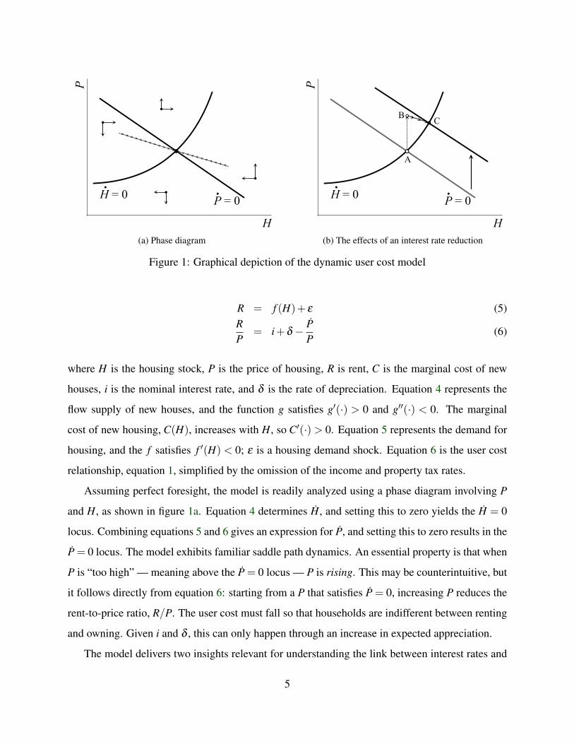
Figure 1: Graphical depiction of the dynamic user cost model
R = f (H)+ ε (5)RP
= i+δ − PP
(6)
where H is the housing stock, P is the price of housing, R is rent, C is the marginal cost of new
houses, i is the nominal interest rate, and δ is the rate of depreciation. Equation 4 represents the
flow supply of new houses, and the function g satisfies g′(·) > 0 and g′′(·) < 0. The marginal
cost of new housing, C(H), increases with H, so C′(·)> 0. Equation 5 represents the demand for
housing, and the f satisfies f ′(H) < 0; ε is a housing demand shock. Equation 6 is the user cost
relationship, equation 1, simplified by the omission of the income and property tax rates.
Assuming perfect foresight, the model is readily analyzed using a phase diagram involving P
and H, as shown in figure 1a. Equation 4 determines H, and setting this to zero yields the H = 0
locus. Combining equations 5 and 6 gives an expression for P, and setting this to zero results in the
P = 0 locus. The model exhibits familiar saddle path dynamics. An essential property is that when
P is “too high” — meaning above the P = 0 locus — P is rising. This may be counterintuitive, but
it follows directly from equation 6: starting from a P that satisfies P = 0, increasing P reduces the
rent-to-price ratio, R/P. The user cost must fall so that households are indifferent between renting
and owning. Given i and δ , this can only happen through an increase in expected appreciation.
The model delivers two insights relevant for understanding the link between interest rates and
5
house prices. One is that with zero expected appreciation, the static user cost relationship, equation
1, applies only to the steady state. Increases in housing demand or the interest rate will shift the
P = 0 locus upward, as shown in figure 1b, and house prices will adjust as the economy moves
to its new steady state. Expected appreciations and depreciations are therefore part of the normal
adjustment process, and do not necessarily imply the existence of bubbles.
A second insight is that interest rate changes cause house prices to overshoot the steady state.
The unanticipated rate reduction depicted in figure 1b, for example, leads to an immediate jump
in house prices (from point A to point B in the diagram), followed by a subsequent decline (from
point B to point C). The initial impact of interest rate changes therefore may exceed what is implied
by the simple user cost model presented in the previous section.
2.3 The credit channel
The stylized user cost framework clearly leaves out a number of other factors that could potentially
affect house prices, and alter prices’ interest rate sensitivity. An obvious omission is the supply of
credit: purchasing a house typically requires a loan, and many households are to some extent con-
strained in terms of the amount they can borrow. While not an explicit part of the framework, the
user cost model is useful for thinking about how this might work. Because borrowing constrained
households face a higher shadow cost of credit, the interest rate that appears in these households’
version of equation 6 exceeds the market interest rate, i. An increase in the availability of credit,
and the relaxation of borrowing constraints, would reduce this shadow cost. The effects would
therefore be similar to those from an interest rate reduction. This is a natural interpretation of
the development of the subprime mortgage market in the U.S., and a plausible story for why that
market’s development was associated with a house price boom. In this interpretation, the price rise
would have been the result of a change in fundamentals, rather than a bubble.
To the extent that expansionary monetary policy relaxes credit constraints, an operative credit
channel would tend to amplify the effects of monetary policy on house prices. According to this
view, a monetary expansion has two effects. The first is to lower the mortgage rate. And second, by
easing the availability of credit, the expansion would also increase the demand for owner-occupied
housing by more than would be implied by the interest rate reduction alone. The P locus would
shift up by a larger amount, amplifying the appreciation.
6
2.4 The risk taking channel
The risk taking channel is a third mechanism through which monetary policy could affect house
prices. According to this view, which has been articulated by Rajan (2005), Borio & Zhu (2008)
and Gambacorta (2009), lower interest rates induce intermediaries to take on additional risk in an
effort to achieve a certain target rate of return. Dell’Ariccia et al. (2010) worked out a partial
equilibrium model in which low interest rates can encourage risk-shifting, and Ioannidou et al.
(2009) presented evidence suggesting that this mechanism was operative for Bolivian banks over
the 1999 to 2003 period. A general theory of interest rates, risk-taking and asset pricing has yet to
be developed, but presumably the increased demand for risky assets caused by low interest rates
would boost the price of risky assets by a larger amount than they would otherwise have risen.
The risk-taking channel maps only loosely into the user cost framework. One interpretation
parallels the credit channel. The increased appetite for risk brought forth by low interest rates
would make intermediaries more willing to lend, increasing credit supply. The increased availabil-
ity of credit would allow some credit-constrained households to purchase homes, thus increasing
the demand for owner-occupied houses and, assuming imperfect substitutability between the two
types of dwellings, decreasing the rent-to-price ratio. An alternative interpretation is that low in-
terest rates somehow reduce σ , the risk premium associated with home ownership. The positive
impact of such a reduction on house prices would be the same an increase in expected home price
appreciation. Neither interpretation implies a bubble.
3 Evidence on the response of house prices to interest rates
This section summarizes the existing literature on the impact of interest rates on house prices,
and presents some new evidence on the relationship between user cost and house prices in the
U.S. from a simple error correction model. Collectively, the results are consistent with an inverse
relationship between house prices and interest rates, but in quantitative terms the effect is modest:
it is considerably weaker than implied by the user cost framework, and insufficient to explain the
magnitude of most countries’ real estate booms.
7

3.1 Existing literature
The cyclical properties of house prices and interest rates are well documented. Claessens et al.
(2011), for example, showed that house prices are strongly procyclical in most countries. Ahearne
et al. (2005) found that low interest rates tend to precede housing price peaks, with a lead of
approximately one to three years. While these patterns are suggestive, discerning the impact of
interest rates per se is complicated by the fact that other macroeconomic factors affecting the
demand for housing are varying along with the interest rate. Moreover, it is impossible to tell from
purely descriptive analysis whether the magnitude of the house price variations are consistent with
the effects implied by user cost theory.
Some indirect evidence on the contribution of interest rates to house price fluctuations was
furnished by Campbell et al. (2009). Using the methodology developed in Campbell (1991), the
authors decomposed house price fluctuations in 23 metropolitan areas in the U.S. into components
attributable to real interest rates, rent, and risk premia. They found that risk premia were the
principal source of variance in U.S. house prices, and that interest rate fluctuations accounted for a
relatively small share.
Another piece of evidence on interest rates’ contribution to house prices, and in particular the
mid-2000 boom, comes from Dokko et al. (2009), who looked at house price forecasts under
alternative interest rate paths, directly addressing Taylor’s (2007, 2009) assertion that overly ex-
pansionary monetary policy caused the boom. They found that deviations from the Taylor rule
explained only a small portion of the pre-crisis rise in property values. Examining nearly 100
years’ worth of data for the U.S., Reinhart & Reinhart (2011) reached a similar conclusion.
A number of recent studies have used vector autoregression (VAR) analysis to estimate the
impact of interest rates on house prices, four of which are summarized in table 1. All four doc-
umented statistically significant effects of monetary policy on house prices, with estimates of the
impact of a 25 basis point monetary policy shock ranging from 0.3% to 0.8%.
Del Negro & Otrok (2007) estimated a six-variable VAR on U.S. data spanning 1986 through
2005. The variables included in the system were the house price, total reserves, CPI inflation, GDP
growth, the 30-year mortgage rate, and the Federal funds rate. Monetary shocks were identified
using sign restrictions, and a novel feature of the analysis is its incorporation of a latent house price
8
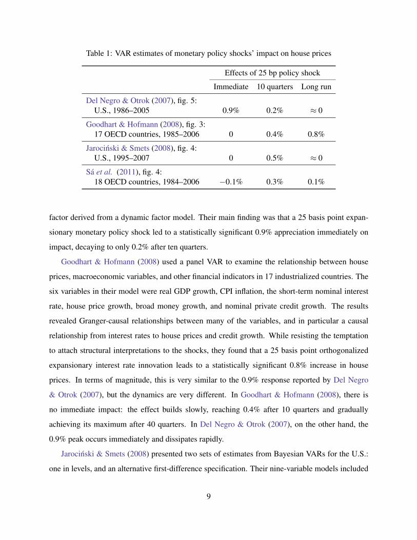
Table 1: VAR estimates of monetary policy shocks’ impact on house prices
Effects of 25 bp policy shock
Immediate 10 quarters Long run
Del Negro & Otrok (2007), fig. 5:U.S., 1986–2005 0.9% 0.2% ≈ 0
Goodhart & Hofmann (2008), fig. 3:17 OECD countries, 1985–2006 0 0.4% 0.8%
Jarocinski & Smets (2008), fig. 4:U.S., 1995–2007 0 0.5% ≈ 0
Sa et al. (2011), fig. 4:18 OECD countries, 1984–2006 −0.1% 0.3% 0.1%
factor derived from a dynamic factor model. Their main finding was that a 25 basis point expan-
sionary monetary policy shock led to a statistically significant 0.9% appreciation immediately on
impact, decaying to only 0.2% after ten quarters.
Goodhart & Hofmann (2008) used a panel VAR to examine the relationship between house
prices, macroeconomic variables, and other financial indicators in 17 industrialized countries. The
six variables in their model were real GDP growth, CPI inflation, the short-term nominal interest
rate, house price growth, broad money growth, and nominal private credit growth. The results
revealed Granger-causal relationships between many of the variables, and in particular a causal
relationship from interest rates to house prices and credit growth. While resisting the temptation
to attach structural interpretations to the shocks, they found that a 25 basis point orthogonalized
expansionary interest rate innovation leads to a statistically significant 0.8% increase in house
prices. In terms of magnitude, this is very similar to the 0.9% response reported by Del Negro
& Otrok (2007), but the dynamics are very different. In Goodhart & Hofmann (2008), there is
no immediate impact: the effect builds slowly, reaching 0.4% after 10 quarters and gradually
achieving its maximum after 40 quarters. In Del Negro & Otrok (2007), on the other hand, the
0.9% peak occurs immediately and dissipates rapidly.
Jarocinski & Smets (2008) presented two sets of estimates from Bayesian VARs for the U.S.:
one in levels, and an alternative first-difference specification. Their nine-variable models included
9

output, consumption, the GDP deflator, housing investment, the house price, the short-term interest
rate, the term spread, a commodity price index, and the money supply. Like Del Negro & Otrok
(2007), they identified structural shocks via sign restrictions on the impulse response functions.
In the levels VAR, an expansionary 25 basis point monetary policy shock leads to a gradual rise
in house prices, peaking at a statistically significant 0.5% after ten quarters. This is accompanied
by a decline in the long-term interest rate of roughly 10 basis points. The effects subsequently
diminish, and 20 quarters after the shock the house price has returned to its mean. The differenced
VAR yielded somewhat larger and more persistent estimates, but the confidence intervals are much
wider, especially at longer horizons.
Finally, a recent paper by Sa et al. (2011) reported panel VAR results for 18 OECD countries
from a 12-variable model, using data from 1984 through 2006. In addition to the standard macro
variables (output, the price level, consumption, non-residential and residential investment, short-
and long-term interest rates, and a measure of credit), the specification also included four variables
reflecting global factors: world GDP, world prices, the trade-weighted exchange rate, and the cur-
rent account balance. Like Del Negro & Otrok (2007) and Jarocinski & Smets (2008), the shocks
were identified using sign restrictions. The results are remarkably similar to those of Jarocinski &
Smets (2008): the response to a 25 basis expansionary shock is initially slightly negative, subse-
quently rising to a statistically significant but modest 0.3% effect after 10 quarters. Over a similar
horizon, the long-term interest rate declines by approximately 10 basis points. Interestingly, the
response is somewhat larger for countries with more sophisticated financial systems (including the
U.S.), where the response at ten quarters is closer to 0.5%. For all countries, the effect subsequently
diminishes, falling to 0.1% after 30 quarters.
These VAR-based estimates are remarkably similar to those reported by Glaeser et al. (2010),
who used a completely different econometric method. Running a simple regression of the log
house price on the real 10-year interest rate, they concluded that a 10 basis point reduction in the
interest rate would result in a 0.7% rise in house prices.
Because it is specified in terms of the long-term interest rate rather than the short-term policy
rate, mapping the Glaeser et al. (2010) figure into the VAR literature requires making an assump-
tion about the effect of policy shocks on longer-term interest rates. An estimate of this effect can
10
be gleaned from the VAR results summarized above: In both Jarocinski & Smets (2008) and Sa
et al. (2011), a 25 basis point expansionary monetary policy shock is associated with a reduction
in the long term interest rate of roughly 10 basis points. This is similar to the results in Kuttner
(2001), which imply a response of approximately 8 basis points. Using the 10 basis point figure as
a rough rule of thumb, the 10 basis point effect implied by the Glaeser et al. (2010) regression is
comparable to the implications of a 25 basis point identified monetary policy shock.
All of these effects are quite modest in economic terms, and considerably smaller than the
effects implied by standard theory. As discussed above in section 2.1, the user cost model suggests
that a 10 basis point reduction in the long-term interest rate, the magnitude typically associated
with a 25 basis point expansionary monetary policy shock, should cause house prices to rise by
1.3% to 1.6%, depending on the initial level of interest rates. By contrast, the VAR estimates,
which range from 0.3% to 0.8%, are one-fourth to one-half the magnitude implied by the user cost
model.
3.2 Results from an error-correction model
While the structural VAR exercises summarized above paid careful attention to the identification of
monetary policy shocks, they failed to incorporate the main features of the user cost model sketched
in section 2.1. If the real UC and expected rate of real appreciation are stationary, equation 1 says
that the rent-to-price ratio should also be stationary. Including rent in the model could therefore
be useful for understanding why macro variables affect the property market, and for determining
whether the observed house price response is excessive relative to the user cost benchmark. This
section presents the results from a simple error-correction model of house prices that represents a
first step in this direction.
But before developing such an error-correction model, one first has to verify that rents and
house prices are indeed cointegrated. As reported in Kuttner (2011b), standard augmented Dicky-
Fuller tests consistently reject the null of non-stationarity for the long of the rent-to-price ratio
calculated using the Freddie Mac FMHPI index for the 1975Q1 to 2011Q1 sample.2 This suggests
2Nonstationarity is also rejected for the discontinued Freddie Mac CMHPI used in Gallin (2008), the FHFA, andthe Census property price indexes. Interestingly, the evidence is weaker for samples ending in the middle of the boomperiod, since at that time property prices had yet to revert to their mean.
11

Figure 2: The effect of a −10 basis point real UC shock on house prices and rents
!"#$%&$'
(&$)&*%
+ , -+ -, .+ ., /+ /,
0+1-
+1+
+1-
+1.
+1/
+1234"'&5($6)&
7&*%
that an error-correction specification would be an appropriate way to model the joint behavior of
rents and house prices. The null hypothesis of nonstationarity is also rejected for the real UC
variable calculated as described in section 2.1, using the 30-year conventional mortgage rate.3
Following Gallin (2008), these considerations led to the specification of a three variable vector
error correction model involving the log of the house price (the FMHPI index), the log of the rent
component of of the CPI, and UC. No attempt is made to identify structural features other than the
long-run relationship implied by the user cost model, so it would be hazardous to attach economic
interpretations to the shocks. The model was estimated with two lags on quarterly U.S. data for the
1984Q1 through 2011Q1 sample period, imposing a cointegrating relationship with coefficients
(1,−1) on the house price and rent variables, and ensuring that the rent-to-price ratio reverts to a
constant mean. Consistent with the cointegration results, the error correction term is significant in
the price (but not the rent) equation; and UC has a negative, statistically significant effect on the
house price.
The most interesting results from the standpoint of this paper have to do with the way in which
house prices and rents react to changes in UC. Figure 2 plots the responses to a 10 basis point
negative real UC innovation: house prices gradually increase, with a maximum response of roughly
3I am indebted to Joshua Gallin for sharing the tax rate and inflation expectations data used in the calculation ofreal UC.
12
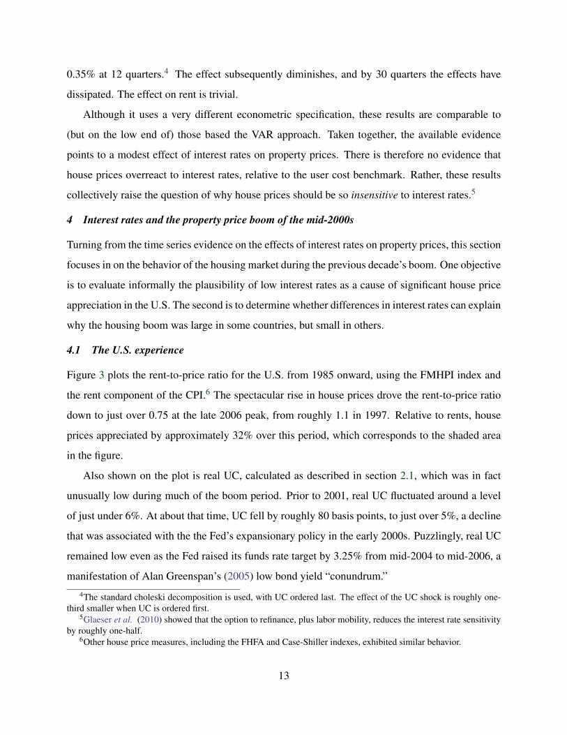
0.35% at 12 quarters.4 The effect subsequently diminishes, and by 30 quarters the effects have
dissipated. The effect on rent is trivial.
Although it uses a very different econometric specification, these results are comparable to
(but on the low end of) those based the VAR approach. Taken together, the available evidence
points to a modest effect of interest rates on property prices. There is therefore no evidence that
house prices overreact to interest rates, relative to the user cost benchmark. Rather, these results
collectively raise the question of why house prices should be so insensitive to interest rates.5
4 Interest rates and the property price boom of the mid-2000s
Turning from the time series evidence on the effects of interest rates on property prices, this section
focuses in on the behavior of the housing market during the previous decade’s boom. One objective
is to evaluate informally the plausibility of low interest rates as a cause of significant house price
appreciation in the U.S. The second is to determine whether differences in interest rates can explain
why the housing boom was large in some countries, but small in others.
4.1 The U.S. experience
Figure 3 plots the rent-to-price ratio for the U.S. from 1985 onward, using the FMHPI index and
the rent component of the CPI.6 The spectacular rise in house prices drove the rent-to-price ratio
down to just over 0.75 at the late 2006 peak, from roughly 1.1 in 1997. Relative to rents, house
prices appreciated by approximately 32% over this period, which corresponds to the shaded area
in the figure.
Also shown on the plot is real UC, calculated as described in section 2.1, which was in fact
unusually low during much of the boom period. Prior to 2001, real UC fluctuated around a level
of just under 6%. At about that time, UC fell by roughly 80 basis points, to just over 5%, a decline
that was associated with the the Fed’s expansionary policy in the early 2000s. Puzzlingly, real UC
remained low even as the Fed raised its funds rate target by 3.25% from mid-2004 to mid-2006, a
manifestation of Alan Greenspan’s (2005) low bond yield “conundrum.”
4The standard choleski decomposition is used, with UC ordered last. The effect of the UC shock is roughly one-third smaller when UC is ordered first.
5Glaeser et al. (2010) showed that the option to refinance, plus labor mobility, reduces the interest rate sensitivityby roughly one-half.
6Other house price measures, including the FHFA and Case-Shiller indexes, exhibited similar behavior.
13
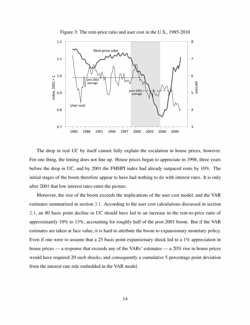
Figure 3: The rent-price ratio and user cost in the U.S., 1985-2010
!"#$%&'())*'+'*
,$-.$
"/
*012 *011 *00* *003 *004 ())) ())5 ())6 ())0
)74
)71
)70
*7)
*7*
*7(
5
3
2
6
4
1
!"#$%&'"(
)#*(+,$-&#%$./'
,$#+0112.3#$.4#
,'"(+0112!"#$!%#
The drop in real UC by itself cannot fully explain the escalation in house prices, however.
For one thing, the timing does not line up. House prices began to appreciate in 1998, three years
before the drop in UC, and by 2001 the FMHPI index had already outpaced rents by 10%. The
initial stages of the boom therefore appear to have had nothing to do with interest rates. It is only
after 2001 that low interest rates enter the picture.
Moreover, the size of the boom exceeds the implications of the user cost model, and the VAR
estimates summarized in section 3.1. According to the user cost calculations discussed in section
2.1, an 80 basis point decline in UC should have led to an increase in the rent-to-price ratio of
approximately 10% to 13%, accounting for roughly half of the post-2001 boom. But if the VAR
estimates are taken at face value, it is hard to attribute the boom to expansionary monetary policy.
Even if one were to assume that a 25 basis point expansionary shock led to a 1% appreciation in
house prices — a response that exceeds any of the VARs’ estimates — a 20% rise in house prices
would have required 20 such shocks, and consequently a cumulative 5 percentage point deviation
from the interest rate rule embedded in the VAR model.
14

Figure 4: Real house prices in selected countries
inde
x,200
3=1
2004 2005 2006 2007 2008 20090.8
1.0
1.2
1.4
1.6
1.8
2.0
2.2
2.4EstoniaIcelandU.S.U.K.KoreaPortugal
4.2 A cross-country exploration
From a global perspective, two observations about the recent real estate boom and bust stand out.
First, the boom was a global phenomenon: most countries experienced rapidly rising real estate
prices during the early and middle part of the last decade. The second observation is that the degree
of appreciation varied widely across countries. This is vividly illustrated in figure 4, which plots
real house prices for six countries: Estonia, Iceland, the U.S., the U.K., Korea, and Portugal, a
set of countries chosen to emphasize the wide variation in the size of the boom. Estonia takes the
prize for the most spectacular bubble, with real house prices in that country increasing by a factor
of nearly 2.4 between the fourth quarter of 2003 and the second quarter of 2007. In comparison
with Estonia, Iceland’s 60% appreciation seems restrained. Both countries’ booms dwarf those of
the U.S. and the U.K., which experienced real house price appreciation over a comparable period
of 17% and 28% respectively.7 House prices barely appreciated at all in Korea, and actually fell
slightly in Portugal.
Some of the cross country differences may be due to discrepancies in the definition and con-
7Note that because these numbers, and figure 4, only cover 2003Q4 through 2007Q2, they understate the size ofthe boom, which began earlier in many countries.
15
struction of the series. Some control for changes in composition (e.g., the repeat sales FMHPI
index in the U.S.) whereas others do not. Moreover, some are national averages, while others, like
Iceland’s, are specific to the capital city. (Details on the house price series used can be found in the
appendix.) It is unlikely that differences in data construction can account for the extreme range of
outcomes across countries, however.
A variety of country- and region-specific factors surely account for much of this diversity.
But in light of concerns about interest rates’ putative contribution to property price bubbles, an
important question is the extent to which differences in interest rates across countries are in any
way related to the relative sizes of the booms. If low interest rates inflate house prices, then one
would expect those countries with lower rates to have experienced more appreciation. And more
broadly, if low interest rates were also associated with more relaxed lending standards and greater
credit supply, as suggested by the credit and risk-taking channels, then low rates would also give
rise to rapid credit growth.
Analogous questions have been examined empirically using the VAR approach surveyed in
section 3.1. Those studies’ emphasis was on the comovements over time between interest rates,
credit, and house prices, however, rather on cross-country differences in the average rates of ap-
preciation that are the focus of this section.8 Here, the aim is to determine the extent to which the
prevailing level of real interest rates were an important determinant of the booms’ relative sizes.
Perhaps the most difficult part of this exercise is obtaining usable property price data. The
primary source of the data used in this analysis is the dataset compiled by the Bank for International
Settlements (BIS). One problem is that many countries, especially transition and emerging market
economies, have only recently begun collecting property price data, which severely constrains
the time series dimension of the analysis. In the end, property price data from 2003Q4 onward
were available for only 36 countries. Details on data sources and definitions can be found in the
appendix.
Another problem is, as noted earlier, that there is no standard methodology for constructing
house price indexes. It therefore goes without saying that the property price levels are not directly
comparable across countries. One has to assume that it is possible to make meaningful comparisons8In panel data parlance, one could say that VAR analysis corresponds loosely to a “within” estimator, whereas the
cross-sectional analysis of averages can be interpreted as a “between” estimator.
16

of the growth rates calculated from these series. Methodological differences will surely introduce
country-specific measurement error, but since property price growth will be used as the dependent
variable in the regressions, the additional noise would increase the regression standard error, but
not bias the parameter estimates.
Finding data on housing-related credit presents another challenge. This paper relies on data
taken from several sources, including the BIS, CEIC, Datastream, and central banks. Cross-country
consistency is again a problem with no clear solution, but as in the case of property prices, there is
reason to believe that any measurement error introduced by methodological differences and other
data issues would increase the standard errors, but not cause bias. Data availability limits to 33 the
number of countries with suitable data from 2003Q4.
Compared with property price and credit data, basic monetary and financial series are relatively
easy to find, as they are available from the IMF’s International Financial Statistics database. Short-
term and lending interest rate series are used, the latter as a proxy for the interest rate that would
be relevant for home purchases. Monetary base data are also obtained form the IMF.9
Histograms of house price growth, credit growth, and interest rates are shown in figures 5 and 6,
distinguished by country group: Eurozone, emerging market, and an “other” category that includes
countries such as U.S., the U.K., Canada, Australia and New Zealand. All figures are calculated
for the 2003Q4 to 2007Q2 time span, the end date corresponding approximately to the housing
market peak.
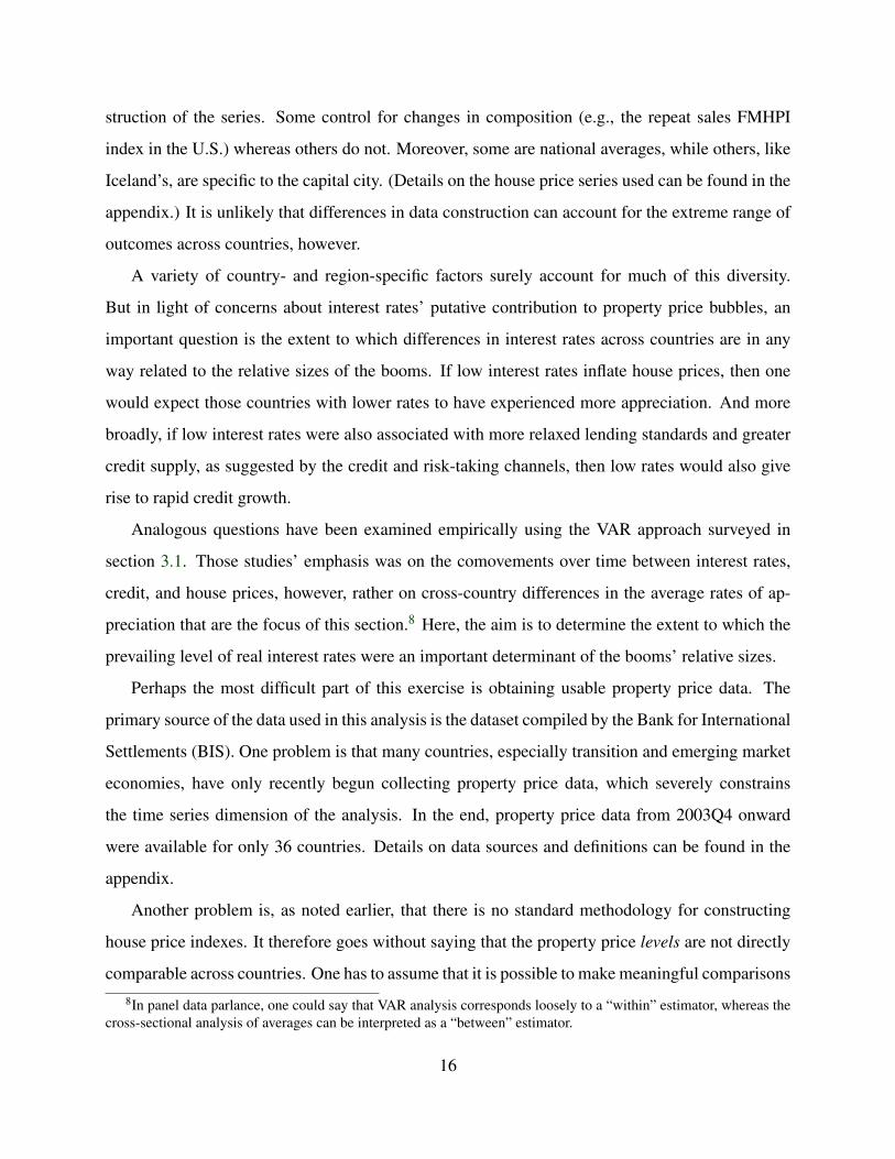
The distribution of house price growth is shown in the top panel of figure 5. Over the 2003Q4 to
2007Q2 period, the majority of countries experienced real property price growth of 5% per year or
more, with many exceeding 10%. Four emerging market economies had real appreciation in excess
of 15% per year. The bottom panel of figure 5 shows the distribution of credit growth, expressed
as the annualized percentage point change in housing credit as a share of GDP. Outcomes here
are similarly varied. The modal growth rates are in the 1–3% range (indicating that housing credit
grew 1–3% more rapidly than GDP), but the rate exceeded 3% in a sizable minority of the countries
in the sample.
As shown in the top panel of figure 6, while relatively low, ex post real short-term interest rates9For Euro area members, the monetary base data reported by the IMF corresponds to the reserves held by the
country’s banking system.
17
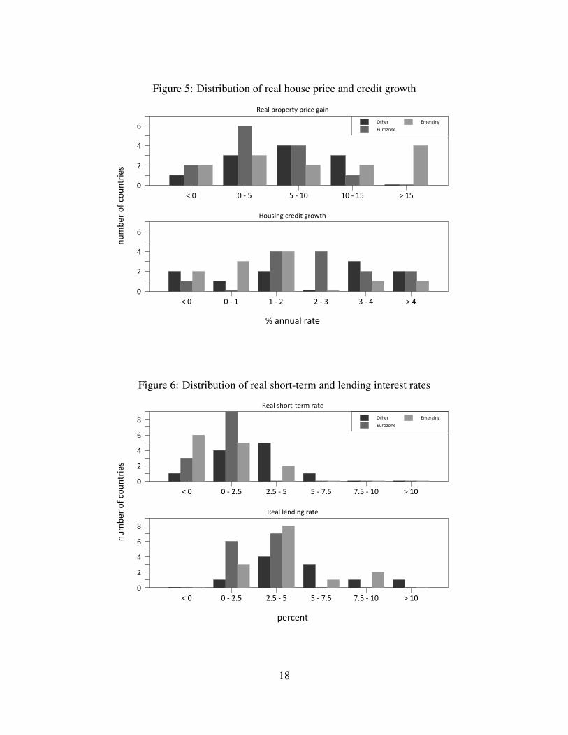
Figure 5: Distribution of real house price and credit growth
!"#$$%#&"'#()
$%*+)'",-".,%$('/)0
1)#&"2',2)'(3"2'/.)"4#/$
5"6 6"7"8 8"7"96 96"7"98 :"98
6
;
<
=>(?)'
@%',A,$)
@*)'4/$4
B,%0/$4".')C/("4',D(?
5"6 6"7"9 9"7"; ;"7"E E"7"< :"<
6
;
<
=
Figure 6: Distribution of real short-term and lending interest rates
!"#$"%&
%'()"#*+,*$+'%&#-".
/"01*.2+#&3&"#(*#0&"
4*5 5*3*678 678*3*8 8*3*978 978*3*:5 ;*:5
5
6
<
=
> ?&2"#
@'#+A+%"
@("#B-%B
/"01*1"%C-%B*#0&"
4*5 5*3*678 678*3*8 8*3*978 978*3*:5 ;*:5
5
6
<
=
>
18
did not vary much across countries. Most fall in the 0–2.5% range, with a few below zero and some
exceeding 2.5%. Real lending rates, shown in the bottom panel, tended to be higher, and most fall
into the 2.5–5% range. Some are lower, but still positive, and a few exceed 5%. The relatively
low dispersion of interest rates alone suggests that they are unlikely to explain much of the cross-
country variation in house price appreciation: property prices would have to be extraordinarily
interest sensitive for changes of one or two percentage points to account for the wildly differing
rates of house price appreciation plotted in figure 5.
A cross-sectional regression model will be used to evaluate the relationship between monetary
conditions and the housing market,
Yi = β0 +β1rLi +β2rS
i +β3%∆MBi +β4Deui +β5Dem
i +ui , (7)
where the dependent variable Y represents either the real property price gain or the growth in
housing credit. The regressors are rS, the average real short-term interest rate; rL, the average real
lending rate; and %∆MB, the annualized average change in the real monetary base. All changes are
calculated over the 2003Q4 to 2007Q2 period. The regression also includes dummies for euro-area
emerging market/transition economies, Deu and Dem.
The inclusion of the monetary base term requires some explanation. Strictly speaking, the
user cost model has no place for monetary quantities, since in the steady state house prices should
be determined solely by rents and interest rates (plus taxes, depreciation, and the risk premium).
However in some countries, base money may serve as a proxy for credit conditions, loosely defined.
A central bank targeting a short-term interest may find itself in a position of having to accommodate
increased credit demand by allowing an expansion in the base, for example. Alternatively, in
countries with actively managed exchange rates, base growth may be associated with unsterilized
capital inflows. Either way, the base may convey some information about the availability of bank
credit beyond that contained in the short-term and lending interest rates.
Many aspects of this regression are problematic, of course. It would be hard to argue that any of
the regressors are exogenous. Since it includes the effects of omitted variables, such as GDP, that
affect property prices and housing credit, these omitted variables’ effects will be subsumed into the
19

Table 2: Results from house price and credit regressions
Dependent variable
Real property Real housingRegressor price growth credit growth
Intercept 9.57∗∗∗ 9.69∗∗∗ 3.33∗∗∗
(2.74) (2.87) (0.81)
Real short-term interest rate 0.37 −0.11(0.89) (0.24)
Real lending rate −1.22 −1.07∗∗ −0.43∗∗
(0.76) (0.54) (0.17)
Real monetary base growth 0.35∗∗∗ 0.36∗∗∗ 0.17∗∗∗
(0.11) (0.11) (0.03)
Emerging market dummy 4.17 2.21 −0.99(3.41) (2.92) (1.10)
Euro area dummy −3.95 −4.34∗ −0.72(2.44) (2.47) (0.84)
p-value for interest rates’ exclusion 0.14 0.05
Adjusted R-squared 0.21 0.19 0.40
Observations 35 36 33
Notes: The table reports the estimates of equation 7. Asterisks denote statis-tical significance: *** for 1%, ** for 5%, and * for 10%, heteroskedasticity-consistent t-statistics are in parentheses.
error term. If the monetary authority takes GDP into account in setting its short-term interest rate
(or if it responds directly to house prices), then the coefficient on the interest rate will be biased. In
addition, the lending rate and monetary base growth are endogenously determined. The regression
is therefore unable to provide a credible answer to counterfactuals involving the likely effect of an
interest rate cut on property prices or credit. At most, it can say something about the expectation
of property prices or credit conditional on the observed behavior of interest rates and the monetary
base.
With these caveats in mind, table 2 displays the results from estimating equation 7. The regres-
sion with real property price growth as the dependent variable, shown in the first column, provides
20

Figure 7: Real monetary base and property price growth
!"#$%&#'"%(!)*+,-%.
,)/'"%0!12"%2,#3("-%.
456 6 56 76 86 96
456
4:
6
:
56
5:
76
7:
86
8:
;+,"!
</!)=)3"
<>"!(13(
New$Zealand
Iceland
Ireland
Slovenia
RussiaEstonia
Latvia
Poland
only weak evidence of an interest rate effect. Neither of the two interest rate coefficients is statisti-
cally significant, nor are they jointly significant. The coefficient on the lending rate does have the
correct sign, however, and with a p-value of 0.11 it is almost significant at the 10% level. Indeed,
if the short-term interest rate is dropped, as in the second column of the table, the coefficient on the
lending rate becomes significant at the 5% level. Even so, the parameter estimate of roughly −1
implies a relatively modest effect: a 1 percentage point increase in the real long-term interest rate
is associated with a 1 percentage point reduction in the annualized real rate of house price appre-
ciation. During normal periods with stable property prices, this would represent a sizable effect.
And taking the estimate at face value, one could point out that a one percentage point increase in
the lending rate in the U.S. would have significantly reduced the annualized growth rate of house
prices from 3.4% to 2.4%. But for countries experiencing double-digit annual growth rates, such
as Estonia and Iceland, a change in the lending rate of a percentage point or two would not have
made a tangible difference.
Interestingly, the coefficient on the monetary base is highly statistically significant, with a 1
percentage point increase in the rate of base growth implying a 0.35% increase in house prices.
21

This may seem like a relatively small effect, and, for those countries with modest rates of real base
growth, it is. But a significant number of countries experienced spectacular real base growth during
this period, including: Iceland (35%), New Zealand (31%), Ireland (26%), Slovenia (24%), Russia
(18%), Estonia (15%) and Latvia (12%). For these countries, the estimated coefficient on the base
growth variable implies quite large effects on property prices. These extreme observations stand
out in figure 7, which plots real house price growth against real base growth, illustrating how rapid
base growth was in some countries accompanied by pronounced house price appreciations.
The third column of table 2 shows an analogous set of estimates for the regression with housing
credit growth (expressed as the percentage point change in the share of housing credit relative to
GDP) as the dependent variable. Here, the lending rate is individually significant at the 5% level,
and the two interest rates are also jointly significant at that level. The −0.43 parameter estimate
says that a 1 percentage point increase in the real lending rate is associated in a 0.43 percentage
point reduction in credit growth. The effect is not large, but with annualized credit growth rates in
the 0 to 4% range, a 1 or 2 percentage point change in the lending rate would make a noticeable
difference.
As in the interest rate regression, the monetary base is highly significant. The point estimate of
0.17 says that a 1 percentage point increase in base growth would translate into a 0.17 percentage
point increase in credit growth. This would not have been a major contributor to credit growth for
those countries with modest rates of base growth. But as with property prices, double-digit growth
in the monetary base in some countries seems to have been associated with sizable increases in
housing-related credit.
5 Conclusions
This paper’s main conclusions are twofold. The first is that all available evidence — existing
studies, plus the new findings presented above — points to a rather small effect of interest rates
on housing prices. VAR-based estimates of the effect of a 25 basis point expansionary monetary
policy shock range from 0.3% to 0.9%, both in the U.S. and in other industrialized countries.
These estimates are broadly consistent with results from other methodologies, including simple
OLS regressions and error-correction models. They are also considerably smaller than the effects
implied by the standard user cost model. Moreover, they are too small to explain the previous
22
decade’s tremendous real estate boom in the U.S. and elsewhere.
This is not to say that low interest rates had nothing to do the real estate boom. The real UC of
home ownership in the U.S. fell by roughly 0.8% after 2001, a change that appears to have been
only partly attributable to monetary policy. If one were to ignore the empirical evidence showing a
much smaller interest sensitivity, taken literally the user cost model could account for roughly half
of the post-2001 house price appreciation. And given that UC did not begin to decline until 2001,
interest rates could not have been a contributor to the the 10% appreciation that occurred before
2001.
But even if a robust inverse relationship between interest rates and house prices existed, it
would not follow from that alone that low interest rates caused bubbles. In the context of standard
theory, the interest rate, along with rents and tax rates, is a fundamental determinant of valuations.
Making the case that low interest rates cause bubbles would require showing that house prices
tend to overreact to rate reductions. Although the previous decade’s house price boom was out of
proportion to the interest rate decline, there is no evidence that this happens systematically. The
puzzle is why house prices are less sensitive to interest rates than theory says they should be, not
more so.
Still lacking is an explanation of why low interest rates sometimes seem to be associated with
bubbles, and sometimes not. The user cost model may contain a clue. As noted earlier, the expected
rate of house price appreciation is an important if unobserved ingredient in user cost. As such, it
is a deus ex machina capable of explaining any level of house prices. But it also suggests that the
interest sensitivity of house prices depends on the expected rate of appreciation, since the interest
semi-elasticity is inversely proportional to user cost. Consequently, in an environment of rapidly
rising house prices, interest rate reductions may have a larger effect than when prices are stable.
Low interest rates may fan the flames, even if they do not start the fire.
The evidence presented in this paper also suggests that credit conditions, broadly defined, may
play a larger role in house price booms than low interest rates per se. In market-oriented financial
systems, like that of the U.S., a loosening of credit conditions plausibly resulted from financial
innovation, such as securitization, and a relaxation of lending standards. In more bank-centric
financial systems, like those present in many emerging market and transition economies, loose
23

credit conditions have been associated with the rapid increase of quantitative monetary indicators,
such as the monetary base. This suggests that it would be a mistake to focus narrowly on interest
rates as the cause of asset price bubbles.
24

Data appendix
The following table lists the countries included in the analysis, details on the property price data,and the data used for the regressions reported in table 2.
House Short- Lend- HousingNew/ price term ing credit Base
Country Region Type existing growth rate rate growth growth
Austria Capital all all 4.2 2.8 4.9 1.80 6.4Australia Big cities all existing 2.1 6.0 9.6 4.19 0.8Belgium Whole all existing 8.2 2.8 5.1 2.38 5.7Canadaa Whole all existing 8.2 3.4 5.2 1.84 1.3Switzerland Whole single family all 0.9 1.0 3.3 1.71 -2.9Colombiab Whole all existing 7.0 7.3 15.3 -0.41 8.0Czech Rep. Whole single family existing 2.5 6.2 1.47 5.7Germanyd Whole all new -1.7 2.7 5.9 -0.33 5.1Denmark Whole all all 12.1 2.9 5.1 2.13 -1.3Estonia Whole flats all 25.3 3.1 5.7 6.70 15.1Spain Whole all all 8.2 2.7 3.9 6.30 8.2Finland Whole all existing 4.9 2.8 3.9 2.66 11.4France Whole all existing 9.9 2.8 5.0 2.58 8.9Great Britain Whole all all 6.0 5.0 4.9 3.55 10.8Greece Capital flats all 3.9 2.8 5.3 3.85 10.6Hong Kong Whole all all 11.6 2.8 7.0 -3.15 -0.6Indonesia Big cities all new -5.3 7.4 15.8 0.25 4.0Ireland Whole all all 3.8 2.8 4.1 6.83 26.1Israel Whole all all -1.3 5.1 7.6 -1.24 -9.9Iceland Capital all all 12.5 10.2 16.4 35.0Italyd Whole all all 4.1 2.8 4.9 1.49 9.3Korea Whole all all 1.1 4.1 6.3 0.90 3.4Latvia Whole flats existing 32.2 2.4 5.9 12.4Lithuania Whole all all 8.8 2.8 4.1 1.78 -4.0Malaysia Whole all all 0.3 3.2 6.6 1.21 4.8Netherlands Whole all existing 2.5 2.8 5.2 1.27 8.5Norway Whole all all 11.0 5.5 4.7 0.31 0.9New Zealand Whole all all 9.1 7.1 11.1 5.98 31.2Poland Big cities flats existing 20.6 5.3 7.3 1.47 8.2Portugal Whole all all -1.1 2.8 4.3 3.56 -7.0Russia Urban areas all existing 22.7 3.5 11.6 18.4Sweden Whole all all 9.2 2.5 3.56 -0.6Singaporec Whole all all 6.8 2.4 5.7 -1.31 6.3Slovenia Whole all existing 13.7 4.2 7.5 23.8Thailandc Whole townhouses all 0.3 3.1 6.8 0.62 -1.0United Statesa Whole single family existing 3.4 3.5 6.7 3.69 -0.3South Africa Whole single family all 14.9 7.8 12.1 4.00 8.4
Notes: property price data are from the BIS except as noted: a, Haver; b, Datastream; c, CEIC.Interpolated series are denoted by d. Interest rates and growth rates are annualized averages over the 2003Q4to 2007Q2, and expressed in real terms, adjusted using CPI inflation.
25
References
Ahearne, Alan, Ammer, John, Doyle, Brian, Kole, Linda, & Martin, Robert. 2005. House Pricesand Monetary Policy: A Cross-Country Study. International Finance Discussion Paper 841.Board of Governors of the Federal Reserve System.
Bernanke, Ben S., & Gertler, Mark. 1999. Monetary Policy and Asset Price Volatility. Pages77–128 of: New Challenges for Monetary Policy. Jackson Hole Symposium. Federal ReserveBank of Kansas City.
Borio, Claudio, & Zhu, Haibin. 2008 (December). Capital regulation, risk-taking and monetarypolicy: a missing link in the transmission mechanism? Working Paper 268. Bank forInternational Settlements.
Campbell, John Y. 1991. A Variance Decomposition for Stock Returns. The Economic Journal,101(405), 157–179.
Campbell, Sean D., Davis, Morris A., Gallin, Joshua, & Martin, Robert F. 2009. What moveshousing markets: A variance decomposition of the rent-price ratio. Journal of UrbanEconomics, 66(2), 90–102.
Claessens, Stijn, Kose, M. Ayhan, & Terrones, Marco E. 2011. Financial Cycles: What? How?When? Working Paper 11/76. International Monetary Fund.
Del Negro, Marco, & Otrok, Christopher. 2007. 99 Luftballons: Monetary policy and the houseprice boom across U.S. states. Journal of Monetary Economics, 54(7), 1962–1985.
Dell’Ariccia, Giovanni, Laeven, Luc, & Marquez, Robert. 2010. Monetary Policy, Leverage, andBank Risk-Taking. Working Paper 10/276. International Monetary Fund.
Dokko, Jane, Doyle, Brian, Kiley, Michael, Kim, Jinill, Sherlund, Shane, Sim, Jae, & Van denHeuvel, Skander. 2009 (December). Monetary Policy and the Housing Bubble. FEDS WorkingPaper 2009-49. Board of Governors of the Federal Reserve System.
Gallin, Joshua. 2008. The Long-Run Relationship Between House Prices and Rents. Real EstateEconomics, 36(4), 635–658.
Gambacorta, Leonardo. 2009. Monetary policy and the risktaking channel. BIS QuarterlyReview, December, 43–53.
Glaeser, Edward L., Gottlieb, Joshua D., & Gyourko, Joseph. 2010 (July). Can Cheap CreditExplain the Housing Boom? Working Paper 16230. National Bureau of Economic Research.
Goodhart, Charles, & Hofmann, Boris. 2008. House prices, money, credit, and themacroeconomy. Oxford Review of Economic Policy, 24(1), 180–205.
Greenspan, Alan. 2005 (February 16). Federal Reserve Board’s semiannual Monetary PolicyReport to the Congress. Testimony Before the Committee on Banking, Housing, and UrbanAffairs, U.S. Senate.
26
Himmelberg, Charles, Mayer, Christopher, & Sinai, Todd. 2005. Assessing High House Prices:Bubbles, Fundamentals and Misperceptions. Journal of Economic Perspectives, 19(4), 67–92.
Ioannidou, Vasso, Ongena, Steven, & Peydro, Jose-Luis. 2009. Monetary Policy, Risk-Taking andPricing: Evidence from a Quasi-Natural Experiment. Working Paper. Tilburg University.
Jarocinski, Marek, & Smets, Frank R. 2008. House Prices and the Stance of Monetary Policy.Federal Reserve Bank of St. Louis Review, 90(July/August), 339–65.
Kuttner, Kenneth N. 2001. Monetary policy surprises and interest rates: Evidence from the Fedfunds futures market. Journal of Monetary Economics, 47(3), 523–44.
Kuttner, Kenneth N. 2011a. Monetary Policy and Asset Price Volatility: Should We Refill theBernanke-Gertler Prescription? Forthcoming in New Perspectives on Asset Price Bubbles:Theory, Evidence, and Policy, Evanoff, Kaufman and Malliaris (eds.), Oxford University Press.
Kuttner, Kenneth N. 2011b (September). Rent, Price, and User Cost in the U.S.: Do the OldRules Still Apply? Unpublished manuscript.
Poterba, James M. 1984. Tax Subsidies to Owner-Occupied Housing: An Asset-MarketApproach. The Quarterly Journal of Economics, 99(4), 729–752.
Rajan, Raghuram G. 2005. Has Financial Development Made the World Riskier? Pages 313–369of: The Greenspan Era: Lessons for the Future. Jackson Hole Symposium. Federal ReserveBank of Kansas City.
Reinhart, Carmen M., & Reinhart, Vincent. 2011 (February). Pride Goes Before a Fall: FederalReserve Policy and Asset Markets. Working Paper 16815. National Bureau of EconomicResearch.
Sa, Filipa, Towbin, Pascal, & Wieladek, Tomasz. 2011 (February). Low Interest Rates andHousing Booms: The Role of Capital Inflows, Monetary Policy, and Financial Innovation.Working paper.
Taylor, John B. 2007 (December). Housing and Monetary Policy. Pages 463–476 of: Housing,Housing Finance and Monetary Policy. Jackson Hole Symposium. Federal Reserve Bank ofKansas City.
Taylor, John B. 2009 (January). The Financial Crisis and the Policy Responses: An EmpiricalAnalysis of What Went Wrong. Working Paper 14631. National Bureau of Economic Research.
27
Related Documents