Low Impact Development Overview Alternative to end of pipe approach to SWM Maintain hydrologic function of local ecosystem Treat stormwater close.
Dec 17, 2015
Welcome message from author
This document is posted to help you gain knowledge. Please leave a comment to let me know what you think about it! Share it to your friends and learn new things together.
Transcript

Low Impact Development OverviewLow Impact Development Overview
Alternative to end of pipe approach to SWM Maintain hydrologic function of local ecosystem Treat stormwater close to the source of runoff Decentralized small scale devices Maintain runoff rates and connection with groundwater
History Prince Georges County Maryland, 1980’s
Means to address economical, environmental and physical shortcomings of traditional stormwater designs
Key Elements Uses common stormwater BMPs Combination of devices results in more efficient land use

LID-EZLID-EZ
Development Similar programs in use in Wake County and Manteo. Local and NC Coastal Federation Funding Cooperation with NC DWQ
Wilmington Version Written to comply with proposed Coastal Rules Quantitative approach to LID developments Based on local ordinances and NC DWQ BMP manual
LID CalculationsLID Calculations
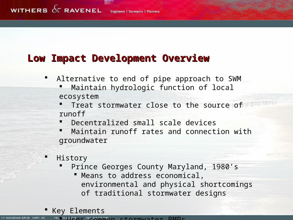
SCS Method Described in TR-55 Per NC DWQ, allowable method for LID Projects only Accounts for soil conditions on site
NC DWQ Involvement No changes required for new Coastal Rules Permitting guidelines in development by DWQ Clarification of policies
Disconnected Impervious Area Pervious Pavement First Flush Calculations

Connected / Disconnected Impervious AreaConnected / Disconnected Impervious Area
Connected Impervious Area Directly connected to drainage conveyance Minimal opportunity for volume reduction before reaching analysis point
Disconnected Impervious Area Runoff has contact with pervious surfaces before reaching analysis point Recommended 50’ sheet flow or sheet flow length equal to width of impervious surface Benefit is dependant on soil type Net result is a reduction of CN

Calculating Runoff Depth, Q [in] – TR-55 Chapter 2Calculating Runoff Depth, Q [in] – TR-55 Chapter 2
Q [in] = (P – Ia)2 / (P + 0.8S),
when (P – Ia) > 0; otherwise Q[in] = 0 in
P = Precipitation depth in inches Ia = Initial hydrologic abstraction = 0.2S S = Potential maximum retention after runoff begins in
inches
S = 1000/CN – 10
Example SiteExample Site
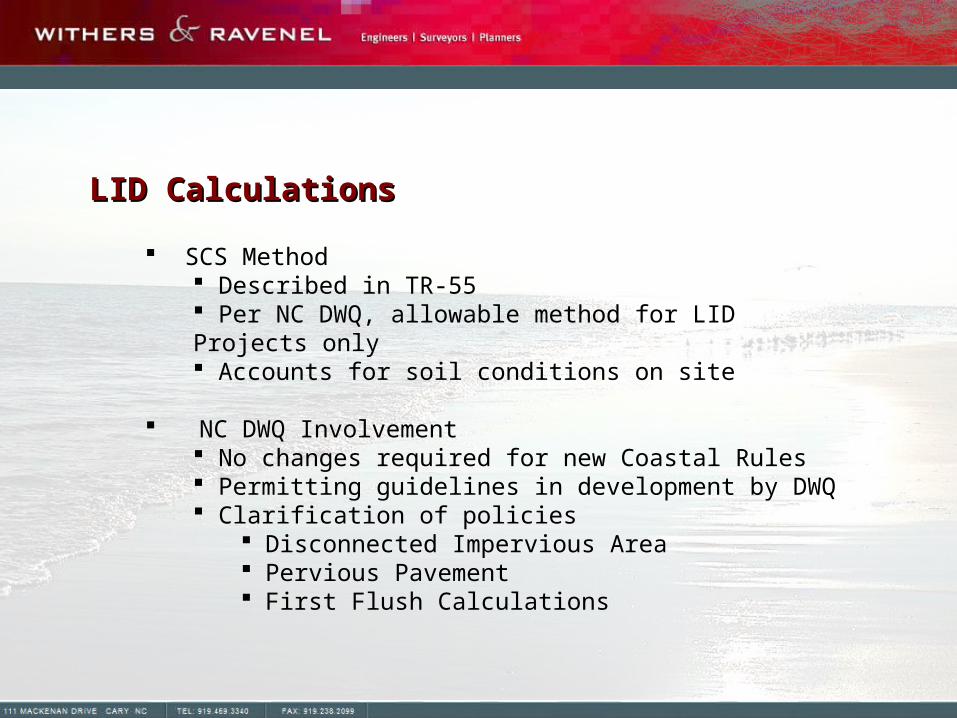
5 acres
– Area = 5.00-ac Single-Family Residential Curb & Gutter 1.6 ac Total Impervious
– 0.85 ac disconnected
Calculating QCalculating Q1-YR 1-YR [in][in]
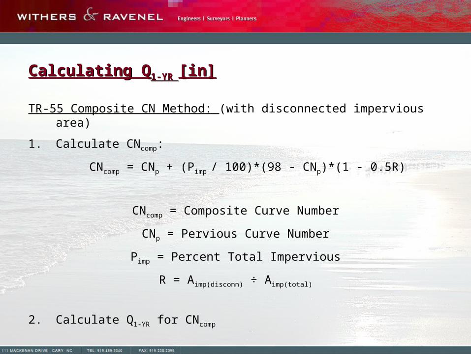
TR-55 Composite CN Method: (with disconnected impervious area)
1. Calculate CNcomp:
CNcomp = CNp + (Pimp / 100)*(98 - CNp)*(1 - 0.5R)
CNcomp = Composite Curve Number
CNp = Pervious Curve Number
Pimp = Percent Total Impervious
R = Aimp(disconn) ÷ Aimp(total)
2. Calculate Q1-YR for CNcomp

CNp = 61 (in this example)
P [in] = 3.41 in (in this example) Pimp = Aimp(tot) ÷ ATot
= (0.75 ac + 0.85 ac) ÷ 5 ac
= 32 % R = Aimp(disconn) ÷ Aimp(total)
= 0.85 ac ÷ 1.60 ac
= 0.53
Calculating QCalculating Q1-YR 1-YR [in] - Continued[in] - Continued

Calculating QCalculating Q1-YR 1-YR [in] - Continued[in] - Continued
CNcomp = CNp + (Pimp / 100)*(98 - CNp)*(1 - 0.5R)
= 61 + (32 / 100)*(98 - 61)*(1 - 0.5*0.53)
= 70
*Note – Without Disconnection CN = 73
S = 1000/CNcomp - 10
= 1000 / 70 - 10
= 4.29 Q1-YR = (P – Ia)2 / (P + 0.8S)
= (3.41 – 0.2*4.29)2 / (3.41 + 0.8*4.29)
= 0.95 in
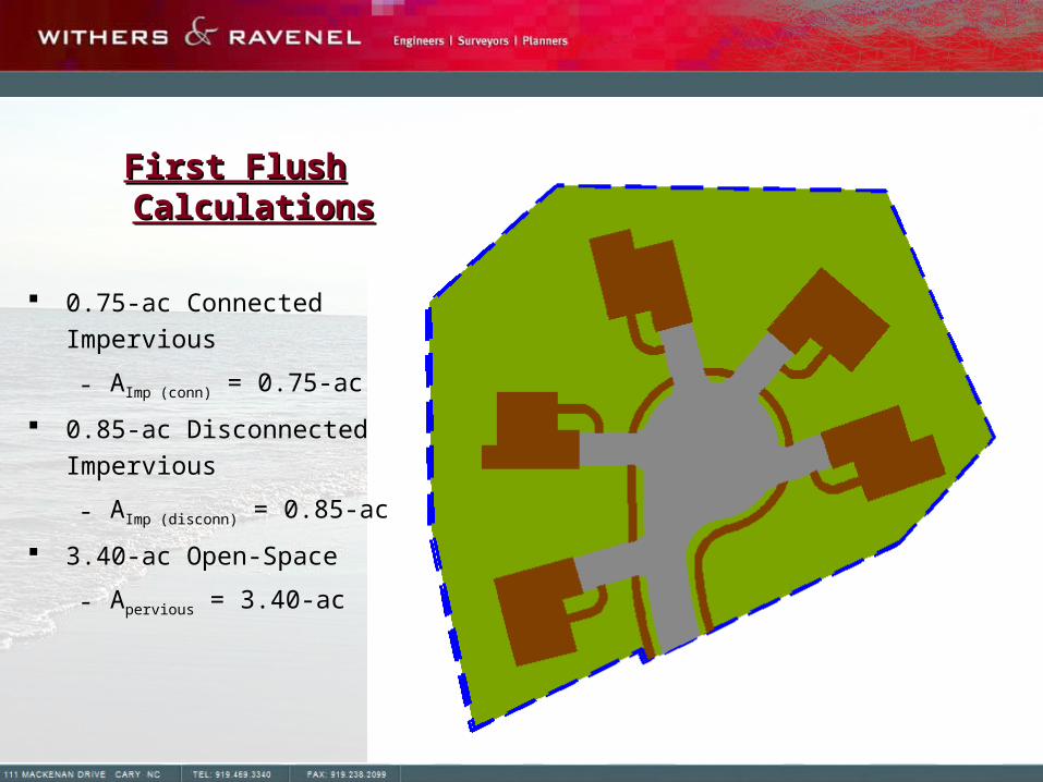
First Flush CalculationsFirst Flush Calculations
0.75-ac Connected Impervious
- AImp (conn) = 0.75-ac
0.85-ac Disconnected
Impervious
- AImp (disconn) = 0.85-ac
3.40-ac Open-Space
- Apervious = 3.40-ac
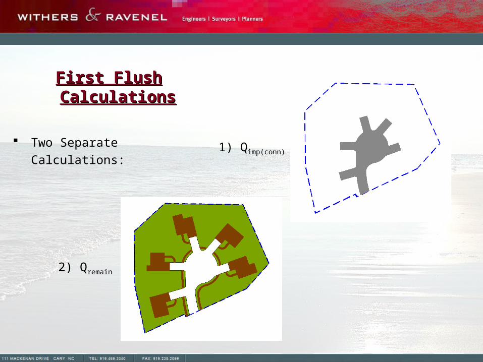
First Flush CalculationsFirst Flush Calculations
Two Separate Calculations:
1) Qimp(conn)
2) Qremain
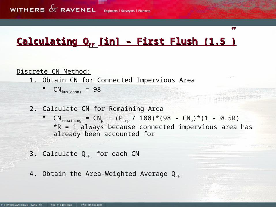
Discrete CN Method:1. Obtain CN for Connected Impervious Area
CNimp(conn) = 98
2. Calculate CN for Remaining Area CNremaining = CNp + (Pimp / 100)*(98 - CNp)*(1 - 0.5R)
*R = 1 always because connected impervious area has already been accounted for
3. Calculate QFF. for each CN
4. Obtain the Area-Weighted Average QFF.
Calculating QCalculating QFF FF [in] – First Flush (1.5”)[in] – First Flush (1.5”)

CNp = 61 (in this example)
P [in] = 1.5 in (in this example) CNimp(conn) = 98
Pimp = Aimp(disconn) ÷ (ATot - Aimp(conn))
= 0.85 ac ÷ (5 ac - 0.75 ac)
= 20 % R = 1
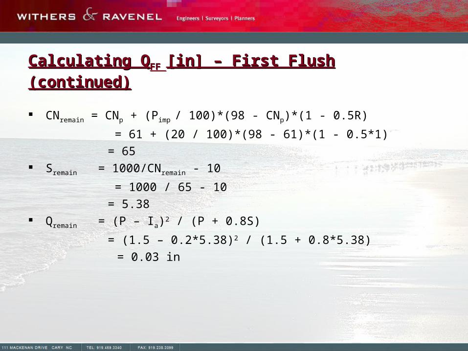
Calculating QCalculating QFF FF [in] – First Flush (continued)[in] – First Flush (continued)
Calculating QCalculating QFF FF [in] – First Flush (continued)[in] – First Flush (continued)
CNremain = CNp + (Pimp / 100)*(98 - CNp)*(1 - 0.5R)
= 61 + (20 / 100)*(98 - 61)*(1 - 0.5*1)
= 65 Sremain = 1000/CNremain - 10
= 1000 / 65 - 10
= 5.38 Qremain = (P – Ia)2 / (P + 0.8S)
= (1.5 – 0.2*5.38)2 / (1.5 + 0.8*5.38)
= 0.03 in

Simp(conn) = 1000/CNimp(conn) - 10
= 1000 / 98 - 10
= 0.20 Qimp(conn) = (P – Ia)2 / (P + 0.8S)
= (1.5 – 0.2*0.20)2 / (1.5 + 0.8*0.20)
= 1.28 in QF.F. = [(QA)remain + (QA)imp(conn)] / ATot
= [(0.03 in * 4.25 ac) + (1.28 in * 0.75 ac)] / 5 ac
= 0.22 in
Calculating QCalculating QFF FF [in] – First Flush (continued)[in] – First Flush (continued)
Storage devices increase effective soil storage capacity, reducing CN
– “Effective Volume” varies based on storm event
– Effective Volume used in Peak Flow calculations Disconnected Impervious Pervious Pavement
– Land Use or Storage Area Lakes and Wetlands
– Coastal Wetlands Pollutant Removal
– BMPs in series
LID-EZ FeaturesLID-EZ Features

LID-EZ – Residential Development - LakesideLID-EZ – Residential Development - Lakeside
Example Site: Lakeside 42.62-ac Parcel “B” Soils
Predevelopment – 100 % Pervious, Natural Area– 35% Open Space, 64% Woods
Post-Development– 24 % Impervious (Lots and Roadways)– 14 % Managed Open-Space
Stormwater Management: 8 Bioretention Cells, 4 Vegetated Swales Total Storage Volume = 167,729 ft3
Total Effective WQV = 33,197 ft3

LID-EZ – Condominium DevelopmentLID-EZ – Condominium Development
Example Site: 9.38-ac Parcel “A” Soils
Predevelopment – 100 % Pervious, Natural Area Post-Development
– 62 % Impervious (Connected)
– 38 % Managed Open-Space
Stormwater Management: 1 Wet Pond, 4 Sand Filters, 6 Infiltration Basins, 1
Bioretention Cell Total Storage Volume = 29,390 ft3

Example Site: House Addition
0.22-ac Lot “A” Soils
Pre-Construction – 21 % Impervious (CN = 52) Post-Construction – 25 % Impervious (CN = 54)
LID-EZ – Quick Calculator – Retrofit SiteLID-EZ – Quick Calculator – Retrofit Site
Related Documents