Low density instability in relativistic mean field models

arX

iv:n

ucl-

th/0

6090

26v1

12

Sep

2006

Low Densities Instability of Relativistic Mean Field Models

A. Sulaksono and T. Mart

Departemen Fisika, FMIPA, Universitas Indonesia, Depok, 16424, Indonesia

Abstract

The effects of the symmetry energy softening of the relativistic mean field (RMF) models on the

properties of matter with neutrino trapping are investigated. It is found that the effects are less

significant than those in the case without neutrino trapping. The weak dependence of the equation

of state on the symmetry energy is shown as the main reason of this finding. Using different

RMF models the dynamical instabilities of uniform matters, with and without neutrino trapping,

have been also studied. The interplay between the dominant contribution of the variation of matter

composition and the role of effective masses of mesons and nucleons leads to higher critical densities

for matter with neutrino trapping. Furthermore, the predicted critical density is insensitive to

the number of trapped neutrinos as well as to the RMF model used in the investigation. It is

also found that additional nonlinear terms in the Horowitz-Piekarewicz and Furnstahl-Serot-Tang

models prevent another kind of instability, which occurs at relatively high densities. The reason is

that the effective σ meson mass in their models increases as a function of the matter density.

PACS numbers: 13.15.+g, 25.30.Pt, 97.60.Jd

1

I. INTRODUCTION

Recently, the dynamical stability of the uniform ground state of multi components sys-

tems (i.e., electrons, protons, and neutrons) at low densities has received considerable atten-

tions [1, 2, 3, 4, 5, 6]. This interest is motivated by the fact that the neutron star is expected

to have a solid inner crust of nonuniform neutron-rich matter above its liquid mantle [3] and

the mass of its crust depends sensitively on the density of its inner edge and on its equation

of state (EOS) [2]. Meanwhile, the critical density (ρc), a density at which the uniform

liquid becomes unstable to a small density fluctuation, can be used as a good approximation

of the edge density of the crust [3]. Using the Skyrme SLy effective interactions, Ref. [2]

found the inner edge of the crust density to be ρedge = 0.08 fm−3. Reference [3] generalized

the dynamical stability analysis of Ref. [7] in order to accommodate the various nonlinear

terms in the relativistic mean field (RMF) model of Horowitz-Piekarewicz [4]. They found

a strong correlation between ρc in neutron star and the symmetry energy (asym) which leads

to a linear relation between ρc and the skin thickness of finite nuclei.

These results suggested that a measurement of the neutron radius in 208Pb will provide

useful information on the ρc [3, 4]. Recently, a new version of the RMF model based on

effective field theory (ERMF) has been proposed by Furnstahl, Serot, and Tang [8]. The

predictive power of the model in a wide range of densities is quite impressive (see the review

articles [9, 10] for the details). On the other hand, an adjustment of the isovector-vector

channel of the ERMF model in order to achieve a softer density dependence of asym at high

densities has been done in Ref. [11].

Similar to the previous calculation done in [4], but using a different RMF model, it is

found that by adjusting that channel a lower proton fraction (Yp) in high density neutron

star matter can be achieved without significantly changing the bulk properties [11]. It is

well known that Yp is related to the threshold of the direct URCA cooling process and

the trend of the density distribution of Yp is unique for each model which is sensitive to

the different forms of nonlinear terms used. Therefore, an investigation of the EOS and

the instability at low densities by using different RMF models could be quite interesting.

Indeed, by comparing our results with the previous ones [3, 4], we can systematically study

the influence of the form and the strength of isovector-vector nonlinear terms on the critical

density. The presence of electrons and the influence of the electromagnetic interaction on

2

the unstable modes of asymmetric matter as well as the comparison between dynamical

instability region with the thermodynamical one have been investigated in Refs. [5, 6] by

using the standard RMF model within the Vlasov formalism. They observed the important

role of the Coulomb field in the large structure formation and also the role of the electron

dynamics in restoring the large-wavelength instabilities [6].

In the actual situation, muons may also be present in the stellar matters. Their existence

yields an additional electromagnetic contribution besides the electrons and protons ones.

The significance of their contribution depends on the matter composition. Including muons

in the dynamical instability analysis of uniform matter increases the electromagnetic effect on

the ρc in medium. Moreover, in supernovae or protoneutron stars neutrinos can be trapped

inside, if their mean free paths are smaller than the star radius. In general, the presence

of trapped neutrinos in matter affects the stiffness of EOS and drastically changes the

composition of neutral matter [12, 13, 14, 15, 16]. It was also found that neutrino trapping

causes the strange baryon [12, 13] and kaon condensate [12, 14] to appear at higher densities

as compared to the case without neutrino trapping. In Ref. [16], the EOS of the strangeness

rich protoneutron star and the EOS of neutron star matter with temperature different from

zero have been already studied by means of the ERMF model. Meanwhile, like neutron stars,

protoneutron stars have dense cores and outer layers [16] and in supernovae inhomogeneity

can appear below the saturation density of nuclear matter (ρ0) [17, 18]. Therefore, an

investigation of the boundary between the two phases, which leads to the determination of

ρc, becomes crucial for a realistic and complete description of stellar matters.

In the present work, we shall extend the analysis of dynamical stability in uniform matter

of Ref. [3] in two ways, i.e., first, we consider the muon contribution and, second, we shall

consider all possible mixings of vector and isovector contributions caused by the nonlinear

terms in the ERMF model. The parameter set NL3 of the standard RMF [19] model as well

as the parameter sets Z271 and Z271* of the Horowitz-Piekarewicz one [4] will be presented

for comparison. The results are used to study the effect of the neutrino presence on the ρc

values. Here, we only use nucleons in the baryonic sector along with σ, ω, and ρ mesons in

the mesonic sector because ρc usually appears at a density lower than ρ0 and the strange

particles appear at a density higher than 2ρ0. Furthermore, in the neutrino trapping case

they appear at higher density than in the case without neutrino trapping. Therefore, we

can assume the strange particles to have only minor effects on the ρc and, as a consequence,

3

their contributions may be neglected in this work. On the other hand, although in the real

situation the temperature of protoneutron stars is not equal to zero and the supernovae inner

core can have a temperature around T ∼ (10-50) MeV, the zero temperature approximation

can be assumed here since the temperature effect on the EOS of supernovae matter and

on the maximum mass of protoneutron star [14, 15] is smaller than that without neutrino

trapping. In this approximation, the following constraints can be used to calculate the

fraction of every constituent in matter:

• balance equation for the chemical potentials

µn + µνe= µp + µe, (1)

• conservation of the charge neutrality

ρe + ρµ = ρp, (2)

where the total density of baryon is given by

ρB = ρn + ρp, (3)

while the fixed electronic-leptonic fraction Yle is defined as

Yle =ρe + ρνe

ρB

≡ Ye + Yνe, (4)

where Yνeand Ye are neutrino electron and electron fractions, respectively. In addition, we

will revisit the EOS of matter with neutrino trapping because we want to study the effect of

different adjustments in the isovector-vector sector [11] on the EOS of matter with neutrino

trapping. They were not fully explored in our previous works [11, 20].

This paper is organized as follows. In Sec. II, a brief review of the model is given.

Calculation of the dielectric function is presented in Sec. III, while numerical results along

with the corresponding discussions are given in Sec. IV. Finally, we give the conclusion in

Sec. V.

II. RELATIVISTIC MEAN FIELD MODELS

Our starting point to describe the non-strange dense stellar matter is an effective La-

grangian density for interacting nucleons, σ, ω, ρ mesons as well as noninteracting leptons.

4

The Lagrangian density for standard RMF models can be found in Refs. [10, 21, 22]. We

note that in order to modify the density dependence of asym, Horowitz-Piekarewicz have

recently added isovector-vector nonlinear terms (LHP) in a standard RMF model [4]. In the

case of ERMF model, the corresponding Lagrangian density can be found in Refs. [8, 11, 23].

For the convenience of the reader, we write the Lagrangian density in a compact form as

L = LN + LM + LHP + LL, (5)

where the nucleon part, up to order ν = 3, reads

LN = ψ[iγµ(∂µ + iνµ + igρbµ + igωVµ) + gAγµγ5aµ

− M + gσσ]ψ −fρgρ

4Mψbµνσ

µνψ, (6)

with

ψ =(p

n

)

, νµ = −i

2(ξ†∂µξ + ξ∂µξ

†) = 통, (7)

aµ = −i

2(ξ†∂µξ − ξ∂µξ

†) = a†µ, (8)

ξ = exp(iπ(x)/fπ), π(x) =1

2~τ · ~π(x), (9)

π(x) =1

2~τ · ~π(x), (10)

bµν = Dµbν −Dν bµ + igρ[bµ, bν ], Dµ = ∂µ + iνµ, (11)

Vµν = ∂µVν − ∂νVµ, (12)

σµν =1

2[γµ, γν ]. (13)

where, p and n are the proton and neutron fields, M is the nucleon mass, while σ, ~π, V µ,

and ~bµ are the σ, π, ω and ρ meson fields, respectively. The meson contribution, up to order

5

ν = 4 is

LM =1

4f 2

πTr(∂µU∂µU †) +

1

4f 2

πTr(U U † − 2) +1

2∂µσ∂

µσ

−1

2Tr(bµν b

µν) −1

4VµνV

µν − gρππ2f 2

π

m2ρ

Tr(bµν νµν)

+1

2

(

1 + η1gσσ

M+η2

2

g2σσ

2

M2

)

m2ωVµV

µ +1

4!ζ0g

2ω(VµV

µ)2

+(

1 + ηρgσσ

M

)

m2ρTr(bµb

µ) −m2σσ

2

(

1 +κ3

3!

gσσ

M+κ4

4!

g2σσ

2

M2

)

, (14)

where

U = ξ2, νµν = ∂µνν − ∂ν νµ + i[νµ, νν ] = −i[aµ, aν ]. (15)

In the mean field approximation, π meson does not contribute. In the Horowitz-Piekarewicz

model [4] the isovector-vector nonlinear term reads

LHP = 4ΛV g2ρg

2ω~bµ ·~bµ V

µVµ. (16)

We note that changing the gρ and ΛV parameters in the Horowitz-Piekarewicz model [4],

or gρ and ηρ parameters in the ERMF model [11], affects the density dependent part of the

asym. A more detailed procedure to adjust the density dependence of the nuclear matter

symmetry energy in RMF models can be found in Refs. [4, 11, 24].

For the leptons, the free Lagrangian density

LL =∑

l=e−, µ−, νe, νµ

l(γµ∂µ −ml)l, (17)

is used. In the present work, the following parameter sets are chosen:

• Standard RMF model: NL3 [19],

• Standard RMF model plus isovector-vector nonlinear term: Z271 and Z271* [4],

• ERMF models: G2 [8] and G2* [11].

The coupling constants for all parameter sets are shown in Table I.

6

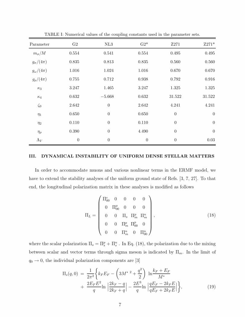
TABLE I: Numerical values of the coupling constants used in the parameter sets.

Parameter G2 NL3 G2* Z271 Z271*

mσ/M 0.554 0.541 0.554 0.495 0.495

gσ/(4π) 0.835 0.813 0.835 0.560 0.560

gω/(4π) 1.016 1.024 1.016 0.670 0.670

gρ/(4π) 0.755 0.712 0.938 0.792 0.916

κ3 3.247 1.465 3.247 1.325 1.325

κ4 0.632 −5.668 0.632 31.522 31.522

ζ0 2.642 0 2.642 4.241 4.241

η1 0.650 0 0.650 0 0

η2 0.110 0 0.110 0 0

ηρ 0.390 0 4.490 0 0

ΛV 0 0 0 0 0.03

III. DYNAMICAL INSTABILITY OF UNIFORM DENSE STELLAR MATTERS

In order to accommodate muons and various nonlinear terms in the ERMF model, we

have to extend the stability analyses of the uniform ground state of Refs. [3, 7, 27]. To that

end, the longitudinal polarization matrix in these analyses is modified as follows

ΠL =

Πe00 0 0 0 0

0 Πµ00 0 0 0

0 0 Πs Πpm Πn

m

0 0 Πpm Πp

00 0

0 0 Πnm 0 Πn

00

, (18)

where the scalar polarization Πs = Πps + Πn

s . In Eq. (18), the polarization due to the mixing

between scalar and vector terms through sigma meson is indicated by Πm. In the limit of

q0 → 0, the individual polarization components are [3]

Πs(q, 0) =1

2π2

{

kFEF −

(

3M∗ 2 +q2

2

)

lnkF + EF

M∗

+2EFE

2

qln

∣∣∣2kF − q

2kF + q

∣∣∣ −

2E3

qln

∣∣∣qEF − 2kFE

qEF + 2kFE

∣∣∣

}

, (19)

7

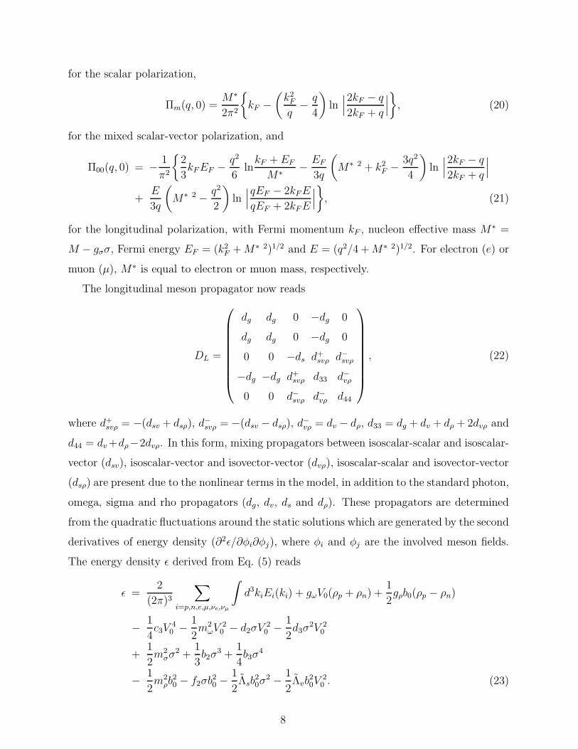
for the scalar polarization,

Πm(q, 0) =M∗

2π2

{

kF −

(k2

F

q−q

4

)

ln∣∣∣2kF − q

2kF + q

∣∣∣

}

, (20)

for the mixed scalar-vector polarization, and

Π00(q, 0) = −1

π2

{2

3kFEF −

q2

6lnkF + EF

M∗−EF

3q

(

M∗ 2 + k2F −

3q2

4

)

ln∣∣∣2kF − q

2kF + q

∣∣∣

+E

3q

(

M∗ 2 −q2

2

)

ln∣∣∣qEF − 2kFE

qEF + 2kFE

∣∣∣

}

, (21)

for the longitudinal polarization, with Fermi momentum kF , nucleon effective mass M∗ =

M − gσσ, Fermi energy EF = (k2F +M∗ 2)1/2 and E = (q2/4 +M∗ 2)1/2. For electron (e) or

muon (µ), M∗ is equal to electron or muon mass, respectively.

The longitudinal meson propagator now reads

DL =

dg dg 0 −dg 0

dg dg 0 −dg 0

0 0 −ds d+svρ d−svρ

−dg −dg d+svρ d33 d−vρ

0 0 d−svρ d−vρ d44

, (22)

where d+svρ = −(dsv + dsρ), d

−svρ = −(dsv − dsρ), d

−vρ = dv − dρ, d33 = dg + dv + dρ + 2dvρ and

d44 = dv +dρ−2dvρ. In this form, mixing propagators between isoscalar-scalar and isoscalar-

vector (dsv), isoscalar-vector and isovector-vector (dvρ), isoscalar-scalar and isovector-vector

(dsρ) are present due to the nonlinear terms in the model, in addition to the standard photon,

omega, sigma and rho propagators (dg, dv, ds and dρ). These propagators are determined

from the quadratic fluctuations around the static solutions which are generated by the second

derivatives of energy density (∂2ǫ/∂φi∂φj), where φi and φj are the involved meson fields.

The energy density ǫ derived from Eq. (5) reads

ǫ =2

(2π)3

∑

i=p,n,e,µ,νe,νµ

∫

d3kiEi(ki) + gωV0(ρp + ρn) +1

2gρb0(ρp − ρn)

−1

4c3V

40 −

1

2m2

ωV20 − d2σV

20 −

1

2d3σ

2V 20

+1

2m2

σσ2 +

1

3b2σ

3 +1

4b3σ

4

−1

2m2

ρb20 − f2σb

20 −

1

2Λsb

20σ

2 −1

2Λvb

20V

20 . (23)

8

From Eq. (23) we can obtain the explicit form of all contributions to the longitudinal

propagator. Note that the energy density of the ERMF model can be obtained from Eq. (23)

by using the following explicit expressions of the coupling constants:

b2 =gσκ3m

2σ

2M, b3 =

g2σκ4m

2σ

6M2, f2 =

gσηρm2ρ

2M,

d2 =gση1m

2ω

2M, d3 =

g2ση2m

2ω

2M2, c3 =

g2ωξ06,

Λs = Λv = 0. (24)

On the other hand, if we set the coupling constants in Eq. (23) to

f2 = d2 = d3 = 0, Λs = 2Λsg2ρg

2σ, Λv = 2Λvg

2ρg

2ω, (25)

we will obtain the energy density of the Horowitz-Piekarewicz model [4]. The mesons effective

masses and the mixing polarizations calculated from the energy density [Eq. (23)] are given

by

m∗ 2σ =

∂2ǫ

∂2σ= m2

σ + 2b2σ + 3b3σ2 − d3V

20 − Λsb

20,

m∗ 2ω = −

∂2ǫ

∂2V0= m2

ω + 2d2σ + d3σ2 + 3c3V

20 + Λvb

20,

m∗ 2ρ = −

∂2ǫ

∂2b0= m2

ρ + 2f2σ + Λsσ2 + ΛvV

20 ,

(26)

and

Π0σω = −

∂2ǫ

∂σ∂V0= 2d2V0 + 2d3σV0,

Π0σρ = −

∂2ǫ

∂σ∂b0= 2f2b0 + 2Λsσb0,

Π00ωρ =

∂2ǫ

∂V0∂b0= −2ΛvV0b0.

(27)

By substituting Eqs. (26) and (27) in the σ, ω, and ρ propagators,

ds =g2

σ(q2 +m∗ 2ω )(q2 +m∗ 2

ρ )

(q2 +m∗ 2ω )(q2 +m∗ 2

ρ )(q2 +m∗ 2σ ) + (Π0

σω)2(q2 +m∗ 2ρ ) + (Π0

σρ)2(q2 +m∗ 2

ω ), (28)

dv =g2

ω(q2 +m∗ 2σ )(q2 +m∗ 2

ρ )

(q2 +m∗ 2ω )(q2 +m∗ 2

ρ )(q2 +m∗ 2σ ) + (Π0

σω)2(q2 +m∗ 2ρ ) − (Π00

ωρ)2(q2 +m∗ 2

σ ), (29)

9

dρ =1/4g2

ρ(q2 +m∗ 2

σ )(q2 +m∗ 2ω )

(q2 +m∗ 2ω )(q2 +m∗ 2

ρ )(q2 +m∗ 2σ ) + (Π0

σρ)2(q2 +m∗ 2

ω ) − (Π00ωρ)

2(q2 +m∗ 2σ )

, (30)

and in the mixing propagators,

dsv =gσgωΠ0

ωσ(q2 +m∗ 2ρ )

H(q, q0 = 0), (31)

dsρ =1/2gρgσΠ0

σρ(q2 +m∗ 2

ω )

H(q, q0 = 0), (32)

dvρ =1/2gρgωΠ00

ωρ(q2 +m∗ 2

σ )

H(q, q0 = 0), (33)

with

H(q, q0 = 0) = (q2 +m∗ 2ω )(q2 +m∗ 2

ρ )(q2 +m∗ 2σ ) + (Π0

σω)2(q2 +m∗ 2ρ )

+ (Π0σρ)

2(q2 +m∗ 2ω ) − (Π00

ωρ)2(q2 +m∗ 2

σ ), (34)

and photon’s propagator

dg =e2

q2, (35)

and using the explicit form of each component, the longitudinal meson propagator can be

obtained.

The explicit derivation of each propagator is given in Appendix A. Note that by setting

all coupling constants in Eqs. (28) - (33) which are not required by the Horowitz-Piekarewicz

model [4] to zero, Eqs. (8), (13) - (14) of Ref. [3] can be obtained.

The uniform ground state system becomes unstable to small-amplitude density fluctua-

tions with momentum transfer q when the following condition is satisfied [3]

det [1 −DL(q)ΠL(q, q0 = 0)] ≤ 0. (36)

The explicit form of Eq. (36) is given in Appendix B. In the case that the density is smaller

than ρ0, the critical density ρc is the largest density for which Eq. (36) has a solution. In

the case that the density is larger than ρ0, if any, ρc is the smallest density.

10

0.0 0.5 1.0 1.5 2.0 2.5 3.0 3.5 4.0 4.5 5.0

B / 0

10-2

10-1

100

101

102

P(M

eVfm

-3)

0 0.1 0.2 0.3 0.4 0.5 0.6 0.7 0.8

(GeV fm-3

)

10-2

10-1

100

101

102

P(M

eVfm

-3)

Z271*Z271NL3G2*G2

0.0 0.5 1.0 1.5 2.0 2.5 3.0 3.5 4.0 4.5 5.0

B / 0

0

50

100

150

200

250

300

350

E/A

(MeV

)

0.0 0.5 1.0 1.5 2.0 2.5 3.0 3.5 4.0 4.5 5.0

B / 0

0.08

0.1

0.12

0.14

0.16

0.18

0.2

Ye

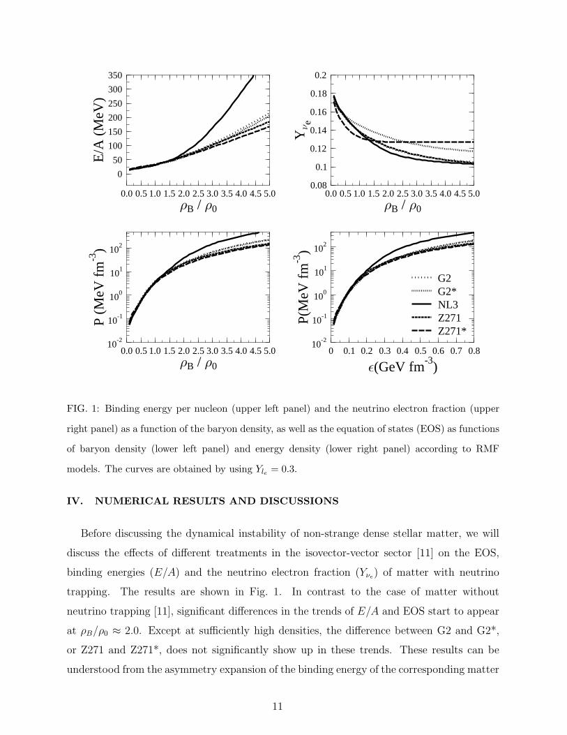
FIG. 1: Binding energy per nucleon (upper left panel) and the neutrino electron fraction (upper

right panel) as a function of the baryon density, as well as the equation of states (EOS) as functions

of baryon density (lower left panel) and energy density (lower right panel) according to RMF

models. The curves are obtained by using Yle = 0.3.

IV. NUMERICAL RESULTS AND DISCUSSIONS

Before discussing the dynamical instability of non-strange dense stellar matter, we will

discuss the effects of different treatments in the isovector-vector sector [11] on the EOS,

binding energies (E/A) and the neutrino electron fraction (Yνe) of matter with neutrino

trapping. The results are shown in Fig. 1. In contrast to the case of matter without

neutrino trapping [11], significant differences in the trends of E/A and EOS start to appear

at ρB/ρ0 ≈ 2.0. Except at sufficiently high densities, the difference between G2 and G2*,

or Z271 and Z271*, does not significantly show up in these trends. These results can be

understood from the asymmetry expansion of the binding energy of the corresponding matter

11

in the vicinity of the symmetric nuclear matter (SNM). The latter is given by [24, 25, 26]

E/A(ρB, α) = (E/A)SNM(ρB, α) + α2asym(ρB)︸ ︷︷ ︸

∆E1/A(ρB ,α)

+ O(α4)︸ ︷︷ ︸

∆E2/A(ρB ,α)

+∆EL/A(ρB), (37)

where α = YN − YP and ∆EL/A is the electrons and muons contribution to the binding

energy. We have found that for all parameter sets and matters used the value of ∆EL/A is

smaller than the other terms. The ∆E2/A term is given by [26]

∆E2/A(ρB, α) = α4Q(ρB) + ... (38)

The origin and connection of the quartic term [Q(ρB)] to direct URCA are discussed in

Ref. [26]. For the case of pure neutron matter (∆E1/A = asym) or other fixed α cases it is

known that ∆E2 ≪ ∆E1. This means that the convergence of the expansion is considerably

fast for these asymmetric matters but for matter with and without neutrino trapping the

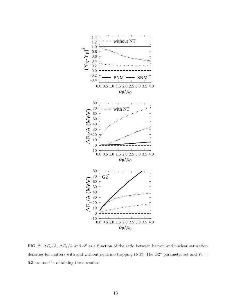
situation is quite different (see Fig. 2). We can see that by imposing the neutrality and β

stability conditions on the matter with and without neutrino trapping, the corresponding

asymmetry (α) becomes density dependent and, evidently, their ∆E2/A are substantially

larger compared to that of the PNM, for example. This indicates that in these cases, the

convergence is significantly slow or even can not be reached at all. Additional constraint in

the form of fixed electronic lepton fraction (Yle) for the case of matter with neutrino trapping

causes the decrease of α2 and the convergence of binding energy expansion are slower than

those in neutrinoless matter.

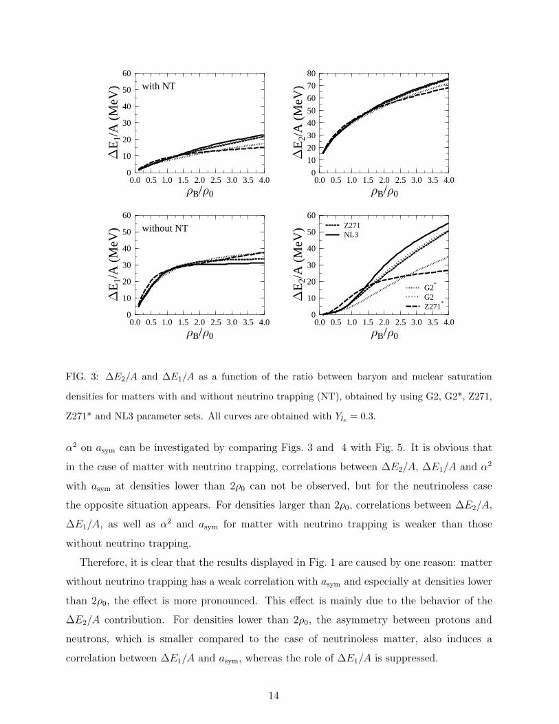
In Fig. 3 we show the ∆E2/A and ∆E1/A as a function of the ratio between baryon and

nuclear saturation densities for the matter with and without neutrino trapping where G2,

G2*, Z271, Z271* and NL3 parameter sets are used. The difference between the two types

of matters appears mainly at densities lower than 2ρ0, where ∆E2/A is smaller than ∆E1/A

for neutrinoless matter. The opposite situation happens for the neutrino trapping case. In

the case of neutrinoless matter and parameter sets with a stiff asym, ∆E2/A is larger than

∆E1/A for the density larger than 2ρ0, but for the case of soft asym this condition is reached

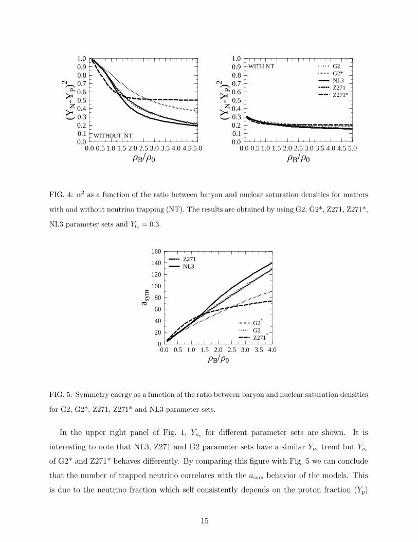
only after the density becomes relatively high. Figure 4 shows the characteristic of α2 for

both matters as the baryon density increases. Here, the dependence of α2 on parameter

sets is obvious for matter without neutrino trapping, while the opposite situation happens

for matter with neutrino trapping. The symmetry energy is shown in Fig. 5, where we can

clearly see its dependence on the parameter sets. The dependency of ∆E2/A, ∆E1/A and

12

0.0 0.5 1.0 1.5 2.0 2.5 3.0 3.5 4.0

B/ 0

-100

1020304050607080

E1/

A(M

eV) G2

*

0.0 0.5 1.0 1.5 2.0 2.5 3.0 3.5 4.0

B/ 0

-100

1020304050607080

E2/

A(M

eV) with NT

0.0 0.5 1.0 1.5 2.0 2.5 3.0 3.5 4.0

B/ 0

-0.4-0.20.00.20.40.60.81.01.21.4

(YN

-YP)

2PNM SNM

without NT

FIG. 2: ∆E2/A, ∆E1/A and α2 as a function of the ratio between baryon and nuclear saturation

densities for matters with and without neutrino trapping (NT). The G2* parameter set and Yle =

0.3 are used in obtaining these results.

13

0.0 0.5 1.0 1.5 2.0 2.5 3.0 3.5 4.0

B/ 0

0

10

20

30

40

50

60

E2/

A(M

eV)

Z271*

G2G2

*

NL3Z271

0.0 0.5 1.0 1.5 2.0 2.5 3.0 3.5 4.0

B/ 0

0

10

20

30

40

50

60

E1/

A(M

eV) without NT

0.0 0.5 1.0 1.5 2.0 2.5 3.0 3.5 4.0

B/ 0

0

10

20

30

40

50

60

70

80

E2/

A(M

eV)

0.0 0.5 1.0 1.5 2.0 2.5 3.0 3.5 4.0

B/ 0

0

10

20

30

40

50

60

E1/

A(M

eV) with NT

FIG. 3: ∆E2/A and ∆E1/A as a function of the ratio between baryon and nuclear saturation

densities for matters with and without neutrino trapping (NT), obtained by using G2, G2*, Z271,

Z271* and NL3 parameter sets. All curves are obtained with Yle = 0.3.

α2 on asym can be investigated by comparing Figs. 3 and 4 with Fig. 5. It is obvious that

in the case of matter with neutrino trapping, correlations between ∆E2/A, ∆E1/A and α2

with asym at densities lower than 2ρ0 can not be observed, but for the neutrinoless case

the opposite situation appears. For densities larger than 2ρ0, correlations between ∆E2/A,

∆E1/A, as well as α2 and asym for matter with neutrino trapping is weaker than those

without neutrino trapping.

Therefore, it is clear that the results displayed in Fig. 1 are caused by one reason: matter

without neutrino trapping has a weak correlation with asym and especially at densities lower

than 2ρ0, the effect is more pronounced. This effect is mainly due to the behavior of the

∆E2/A contribution. For densities lower than 2ρ0, the asymmetry between protons and

neutrons, which is smaller compared to the case of neutrinoless matter, also induces a

correlation between ∆E1/A and asym, whereas the role of ∆E1/A is suppressed.

14

0.0 0.5 1.0 1.5 2.0 2.5 3.0 3.5 4.0 4.5 5.0

B/ 0

0.00.10.20.30.40.50.60.70.80.91.0

(YN

-YP)

2

WITHOUT NT

0.0 0.5 1.0 1.5 2.0 2.5 3.0 3.5 4.0 4.5 5.0

B/ 0

0.00.10.20.30.40.50.60.70.80.91.0

(YN

-YP)

2

Z271*Z271NL3G2*G2WITH NT

FIG. 4: α2 as a function of the ratio between baryon and nuclear saturation densities for matters

with and without neutrino trapping (NT). The results are obtained by using G2, G2*, Z271, Z271*,

NL3 parameter sets and Yle = 0.3.

0.0 0.5 1.0 1.5 2.0 2.5 3.0 3.5 4.0

B/ 0

0

20

40

60

80

100

120

140

160

a sym

Z271*

G2G2

*

NL3Z271

FIG. 5: Symmetry energy as a function of the ratio between baryon and nuclear saturation densities

for G2, G2*, Z271, Z271* and NL3 parameter sets.

In the upper right panel of Fig. 1, Yνefor different parameter sets are shown. It is

interesting to note that NL3, Z271 and G2 parameter sets have a similar Yνetrend but Yνe

of G2* and Z271* behaves differently. By comparing this figure with Fig. 5 we can conclude

that the number of trapped neutrino correlates with the asym behavior of the models. This

is due to the neutrino fraction which self consistently depends on the proton fraction (Yp)

15

0.0 0.2 0.4 0.6 0.8 1.0 1.2 1.4

B / 0

10-2

10-1

100

101

P(M

eVfm

-3)

G2*

0 40 80 120 160 200

( MeV fm-3

)

10-2

10-1

100

101

P(M

eVfm

-3)

Y e=0Yle=0.5Yle=0.4Yle=0.3

0.0 0.5 1.0 1.5 2.0 2.5 3.0 3.5 4.0 4.5 5.0

B / 0

0

50

100

150

200

250

300

350

E/A

(MeV

)

0.0 0.5 1.0 1.5 2.0 2.5 3.0 3.5 4.0 4.5 5.0

B / 0

0.00.020.040.060.08

0.10.120.140.160.180.2

Ye

FIG. 6: Same as Fig. 1, but here the Yle is varied and the G2∗ parameter set is used.

through the neutrality and beta equilibrium conditions, while Yp has a correlation with asym,

although the effect is quite small for this kind of matter.

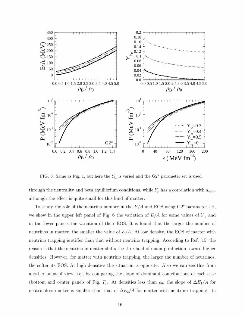
To study the role of the neutrino number in the E/A and EOS using G2∗ parameter set,

we show in the upper left panel of Fig. 6 the variation of E/A for some values of Yle and

in the lower panels the variation of their EOS. It is found that the larger the number of

neutrinos in matter, the smaller the value of E/A. At low density, the EOS of matter with

neutrino trapping is stiffer than that without neutrino trapping. According to Ref. [15] the

reason is that the neutrino in matter shifts the threshold of muon production toward higher

densities. However, for matter with neutrino trapping, the larger the number of neutrinos,

the softer its EOS. At high densities the situation is opposite. Also we can see this from

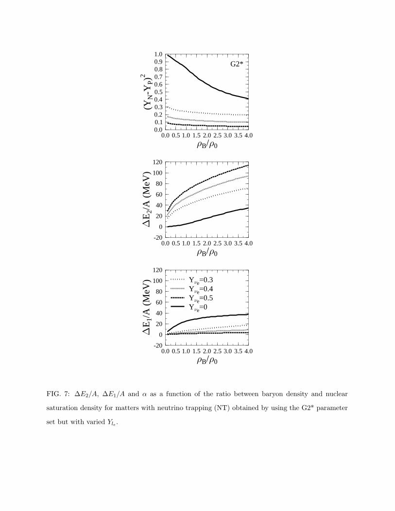
another point of view, i.e., by comparing the slope of dominant contributions of each case

(bottom and center panels of Fig. 7). At densities less than ρ0, the slope of ∆E1/A for

neutrinoless matter is smaller than that of ∆E2/A for matter with neutrino trapping. In

16

0.0 0.5 1.0 1.5 2.0 2.5 3.0 3.5 4.0

B/ 0

-20

0

20

40

60

80

100

120

E1/

A(M

eV)

Y e=0Y e=0.5Y e=0.4Y e=0.3

0.0 0.5 1.0 1.5 2.0 2.5 3.0 3.5 4.0

B/ 0

-20

0

20

40

60

80

100

120

E2/

A(M

eV)

0.0 0.5 1.0 1.5 2.0 2.5 3.0 3.5 4.0

B/ 0

0.00.10.20.30.40.50.60.70.80.91.0

(YN

-YP)

2

G2*

FIG. 7: ∆E2/A, ∆E1/A and α as a function of the ratio between baryon density and nuclear

saturation density for matters with neutrino trapping (NT) obtained by using the G2* parameter

set but with varied Yle .

Ye 0.25 0.3 0.35 0.4 0.45 0.5

Yle

0.00.10.20.30.40.50.60.70.80.91.0

c/

0

G2

Ye 0.25 0.3 0.35 0.4 0.45 0.5

Yle

0.00.10.20.30.40.50.60.70.80.91.0

c/

0

G2*

Ye 0.25 0.3 0.35 0.4 0.45 0.5

Yle

0.00.10.20.30.40.50.60.70.80.91.0

c/

0

Z271

Ye 0.25 0.3 0.35 0.4 0.45 0.5

Yle

0.00.10.20.30.40.50.60.70.80.91.0

c/

0

Z271*

FIG. 8: Critical densities for the Z271, Z271*, G2 and G2* parameter sets as a function of the

neutrino fraction in matter.

the latter, also in the same density range, even though it does not clearly visible, the slope

becomes larger as Yle becomes larger. The situation is reversed once the densities become

higher than ρ0.

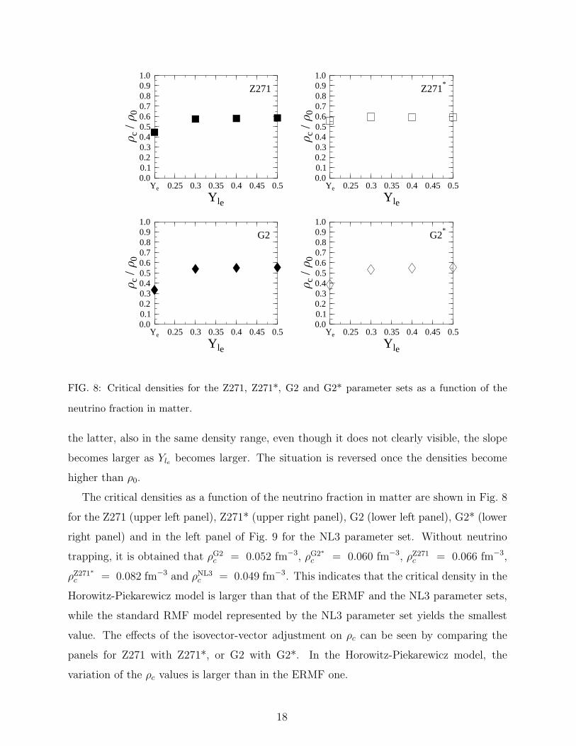
The critical densities as a function of the neutrino fraction in matter are shown in Fig. 8

for the Z271 (upper left panel), Z271* (upper right panel), G2 (lower left panel), G2* (lower

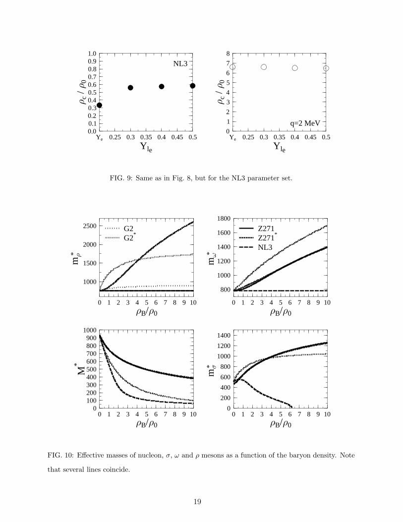
right panel) and in the left panel of Fig. 9 for the NL3 parameter set. Without neutrino

trapping, it is obtained that ρG2c = 0.052 fm−3, ρG2∗

c = 0.060 fm−3, ρZ271c = 0.066 fm−3,

ρZ271∗

c = 0.082 fm−3 and ρNL3c = 0.049 fm−3. This indicates that the critical density in the

Horowitz-Piekarewicz model is larger than that of the ERMF and the NL3 parameter sets,

while the standard RMF model represented by the NL3 parameter set yields the smallest

value. The effects of the isovector-vector adjustment on ρc can be seen by comparing the

panels for Z271 with Z271*, or G2 with G2*. In the Horowitz-Piekarewicz model, the

variation of the ρc values is larger than in the ERMF one.

18

Ye 0.25 0.3 0.35 0.4 0.45 0.5

Yle

0.00.10.20.30.40.50.60.70.80.91.0

c/

0

NL3

Ye 0.25 0.3 0.35 0.4 0.45 0.5

Yle

0

1

2

3

4

5

6

7

8

c/

0

q=2 MeV

FIG. 9: Same as in Fig. 8, but for the NL3 parameter set.

0 1 2 3 4 5 6 7 8 9 10

B/ 0

0100200300400500600700800900

1000

M*

0 1 2 3 4 5 6 7 8 9 10

B/ 0

0

200

400

600

800

1000

1200

1400

m*

0 1 2 3 4 5 6 7 8 9 10

B/ 0

1000

1500

2000

2500

m*

G2*

G2

0 1 2 3 4 5 6 7 8 9 10

B/ 0

800

1000

1200

1400

1600

1800m

*

NL3Z271

*Z271

FIG. 10: Effective masses of nucleon, σ, ω and ρ mesons as a function of the baryon density. Note

that several lines coincide.

19

On the other hand, with neutrino trapping we obtain, ρG2c = (0.084 − 0.086) fm−3,

ρG2∗

c = (0.083−0.086) fm−3, ρZ271c = (0.085−0.086) fm−3, ρZ271∗

c = (0.087−0.088) fm−3

and ρNL3c = (0.081− 0.084) fm−3. This indicates that for this case the value of ρc does not

sensitively depend on the model and on the variation of the number of trapped neutrinos in

matter. In general, their values are larger than those obtained in the case without neutrino

trapping.

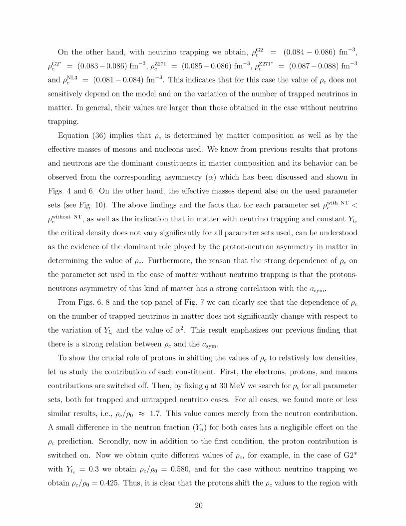
Equation (36) implies that ρc is determined by matter composition as well as by the

effective masses of mesons and nucleons used. We know from previous results that protons

and neutrons are the dominant constituents in matter composition and its behavior can be

observed from the corresponding asymmetry (α) which has been discussed and shown in

Figs. 4 and 6. On the other hand, the effective masses depend also on the used parameter

sets (see Fig. 10). The above findings and the facts that for each parameter set ρwith NTc <

ρwithout NTc , as well as the indication that in matter with neutrino trapping and constant Yle

the critical density does not vary significantly for all parameter sets used, can be understood

as the evidence of the dominant role played by the proton-neutron asymmetry in matter in

determining the value of ρc. Furthermore, the reason that the strong dependence of ρc on

the parameter set used in the case of matter without neutrino trapping is that the protons-

neutrons asymmetry of this kind of matter has a strong correlation with the asym.

From Figs. 6, 8 and the top panel of Fig. 7 we can clearly see that the dependence of ρc

on the number of trapped neutrinos in matter does not significantly change with respect to

the variation of Yle and the value of α2. This result emphasizes our previous finding that

there is a strong relation between ρc and the asym.

To show the crucial role of protons in shifting the values of ρc to relatively low densities,

let us study the contribution of each constituent. First, the electrons, protons, and muons

contributions are switched off. Then, by fixing q at 30 MeV we search for ρc for all parameter

sets, both for trapped and untrapped neutrino cases. For all cases, we found more or less

similar results, i.e., ρc/ρ0 ≈ 1.7. This value comes merely from the neutron contribution.

A small difference in the neutron fraction (Yn) for both cases has a negligible effect on the

ρc prediction. Secondly, now in addition to the first condition, the proton contribution is

switched on. Now we obtain quite different values of ρc, for example, in the case of G2*

with Yle = 0.3 we obtain ρc/ρ0 = 0.580, and for the case without neutrino trapping we

obtain ρc/ρ0 = 0.425. Thus, it is clear that the protons shift the ρc values to the region with

20

relatively low densities. Next, the electron contribution is switched on. Then we observed

that ρc/ρ0 is shifted further, i.e., ρc/ρ0 = 0.430 for Yle = 0.3 and ρc/ρ0 = 0.350 for matter

without neutrino trapping. If the muons contribution is switched on, the result does not

change. It happens not only in matter with neutrino trapping, but also in matter without

neutrino trapping, respectively. However, these results show that the proton and electron

contributions decrease the value of ρc in different ways for both cases and, therefore, reveal

the crucial role of matter composition in determining the value of ρc.

In contrast to the Horowitz-Piekarewicz and ERMF models, the NL3 parameter set yields

an additional instability at relatively high densities. This is shown in the right panel of Fig. 9

for the q = 2 MeV case, i.e., ρc/ρ0 ≈ 6.5. Even if we use q close to zero, this instability does

not disappear and the ρc/ρ0 value stays similar as in the q = 2 MeV case. Therefore, this

instability is not due to the small-amplitude density fluctuations. In fact, this instability

appears because the effective σ mass of the NL3 parameter set is zero at that density (as

shown in the lower right panel of Fig. 10). As a consequence, the corresponding σ propagator

changes the sign at this point. This fact clearly shows that additional nonlinear terms to the

σ nonlinearities of the standard RMF models like in the Horowitz-Piekarewicz and ERMF

ones can prevent such kind of instability to appear.

V. CONCLUSION

The effects of the different treatments in the isovector-vector sector of RMF models on

the properties of matter with neutrino trapping have been studied. The effects are less

significant compared to those without neutrino trapping. Different dependences of the EOS

and B/A of both matters on asym are the reason behind this.

The effects of the variation of the neutrino fraction in matter on the EOS and B/A have

been also discussed.

The longitudinal dielectric function of the ERMF model for matter consisting of neutrons,

protons, electrons, muons, and neutrinos has been derived. The result is used to study the

dynamical instability of uniform matters at low densities. The behavior of the predicted

ρc in matter with and without neutrino trapping has been investigated. It is found that

different treatments in the isovector-vector sector of RMF models yield more substantial

effects in matter without neutrino trapping rather than in matter with neutrino trapping.

21

Moreover, for matter with neutrino trapping, the value of ρc does not significantly change

with the variation of the models as well as with the variation of the neutrino fraction in

matter. In this case, the value of ρc is larger for matter with neutrino trapping. These

are due to the interplay between the major role of matter composition and the role of the

effective masses of mesons and nucleons. It is also found that the additional nonlinear terms

of Horowitz-Piekarewicz and ERMF models prevent another instability at relatively high

densities to appear. This can be traced back to the effective σ mass which goes to zero when

the density approaches 6.5 ρ0 .

ACKNOWLEDGMENT

We are indebted to Marek Nowakowski for useful suggestions and proofreading this

manuscript. We also acknowledge the support from the Hibah Pascasarjana grant as well

as from the Faculty of Mathematics and Sciences, University of Indonesia.

APPENDIX A: MESON PROPAGATORS

In this Appendix, simplified Dyson equations for meson propagators (only zero component

of each propagator is considered) will be given. The covariant form for σ and ω couplings is

given in Ref. [28]. If we define the σ, ω and ρ free propagators as

Gσ =i

q2µ −m2

σ

G00ω =

−i

q2µ −m2

ω

G00ρ =

−i

q2µ −m2

ρ

, (A1)

the Dyson equation for the σ propagator in the absence of coupling to ω and ρ fields is

obtained by considering the sum of ring diagrams, i.e.,

Gσ = Gσ − iGσΠσσGσ, (A2)

from which we can obtain

Gσ =Gσ

1 + iΠσσGσ=

i

q2µ − (m∗

σ)2. (A3)

Similarly, the Dyson equations for the zero components of ω and ρ meson propagators are

G00ω =

G00ω

1 − iΠ00ωωG

00ω

=−i

q2µ − (m∗

ω)2, (A4)

22

and

G00ρ =

G00ρ

1 − iΠ00ρρG

00ρ

=−i

q2µ − (m∗

ρ)2, (A5)

where (m∗σ)2= (mσ)2 +Πσσ, (m∗

ω)2= (mω)2 +Π00ωω, and (m∗

ρ)2= (mρ)

2 +Π00ρρ.

In the ERMF model, each meson is coupled to other mesons through the nonlinear terms.

This fact further complicates the form of the full propagators. The Dyson equation for the

σ propagator including the possible mixing terms becomes

Gσ = Gσ − GσΠ0σωG

00ω Π0

σωGσ − GσΠ0σρG

00ρ Π0

σρGσ, (A6)

which can be written as

Gσ =Gσ

1 + Gσ(Π0σωG

00ω Π0

σω + Π0σρG

00ρ Π0

σρ). (A7)

Equation (A7) can be simplified into

Gσ =i(q2

µ −m∗ 2ω )(q2

µ −m∗ 2ρ )

(q2µ −m∗ 2

ω )(q2µ −m∗ 2

ρ )(q2µ −m∗ 2

σ ) + (Π0σω)2(q2

µ −m∗ 2ρ ) + (Π0

σρ)2(q2

µ −m∗ 2ω )

. (A8)

Similarly, the zero component of ω and ρ meson propagators can be written as

G00ω =

−i(q2µ −m∗ 2

σ )(q2µ −m∗ 2

ρ )

(q2µ −m∗ 2

ω )(q2µ −m∗ 2

ρ )(q2µ −m∗ 2

σ ) + (Π0σω)2(q2

µ −m∗ 2ρ ) − (Π00

ωρ)2(q2

µ −m∗ 2σ )

, (A9)

and

G00ρ =

−i(q2µ −m∗ 2

σ )(q2µ −m∗ 2

ω )

(q2µ −m∗ 2

ω )(q2µ −m∗ 2

ρ )(q2µ −m∗ 2

σ ) + (Π0σρ)

2(q2µ −m∗ 2

ω ) − (Π00ωρ)

2(q2µ −m∗ 2

σ ). (A10)

We can also define a propagator G0ωσ which contains the sum of all diagrams that transform

ω into σ, i.e.,

G0ωσ = −iG00

ω Π0ωσGσ + iG00

ω Π0ωσGσΠ

0σωG

00ω Π0

ωσGσ + · · ·

+ iG00ω Π0

ωσGσΠ0σρG

00ρ Π0

ρσGσ + · · · + iG00ω Π0

ωρG00ρ Π0

ρωG00ω Π0

ωσGσ + · · ·

+ · · ·. (A11)

This propagator may be summed up to produce

G0ωσ =

−iG00ω Π0

ωσGσ

1 + GσΠ0σωG

00ω Π0

ωσ + GσΠ0σρG

00ρ Π0

ρσ + G00ω Π00

ωρG00ρ Π00

ρω

, (A12)

which can be simplified to

G0ωσ =

−iΠ0ωσ(q2

µ −m∗ 2ρ )

H(q, q0). (A13)

23

Similarly, we can also obtain the sum of all diagrams that transform ρ into σ as

G0ρσ =

−iΠ0ρσ(q2

µ −m∗ 2ω )

H(q, q0), (A14)

and that transform ρ into ω as

G00ρω =

iΠ00ρω(q2

µ −m∗ 2σ )

H(q, q0), (A15)

where

H(q, q0) = (q2µ −m∗ 2

ω )(q2µ −m∗ 2

ρ )(q2µ −m∗ 2

σ ) + (Π0σω)2(q2

µ −m∗ 2ρ ) + (Π0

σρ)2(q2

µ −m∗ 2ω )

− (Π00ωρ)

2(q2µ −m∗ 2

σ ). (A16)

Equations (28) - (33) are special cases of Eqs. (A8 - A10, A13, A14, A15), i.e. by taking the

limit of q0 → 0 and inserting the proper mesons coupling constants in the latter.

APPENDIX B: EXPLICIT FORM OF THE LONGITUDINAL DIELECTRIC

FUNCTION

In this Appendix, the explicit form of the longitudinal dielectric function ǫL =

[1 −DL(q)ΠL(q, q0 = 0)] is provided. If we define the matrix ǫL as

ǫL =

A1 B1 D1 E1 F1

A2 B2 D2 E2 F2

A4 B4 D4 E4 F4

A5 B5 D5 E5 F5

A6 B6 D6 E6 F6

, (B1)

then the contents of each component of the matrix in Eq. (B1) are

A1 = 1 − dgΠe00, A2 = − dgΠ

e00, A4 = 0,

B1 = − dgΠµ00, B2 = 1 − dgΠ

µ00, B4 = 0,

D1 = dgΠpm, D2 = dgΠ

pm, D4 = 1 + dsΠs − d+

svρΠpm − d−svρΠ

nm,

E1 = dgΠp00, E2 = dgΠ

p00, E4 = dsΠ

pm − d+

svρΠp00,

F1 = 0, F2 = 0, F4 = dsΠnm − d−svρΠ

n00,

(B2)

24

and

A5 = dgΠe00, A6 = 0,

B5 = dgΠµ00, B6 = 0,

D5 = −d+svρΠs − d33Π

pm − d−vρΠ

nm, D6 = −d−svρΠs − d−vρΠ

pm − d44Π

nm,

E5 = 1 − d+svρΠ

pm − d33Π

p00, E6 = −d−svρΠ

pm − d−vρΠ

p00,

F5 = −d+svρΠ

nm − d−vρΠ

n00, F6 = 1 − d−svρΠ

nm − d44Π

n00.

(B3)

[1] C.J. Pethick, D. G. Ravenhall, and C. P. Lorenz, Nucl. Phys. A 584, 675 (1995).

[2] F. Douchin, and P. Haensel, Phys. Lett. B 485, 107 (2001).

[3] J. Carriere, C. J. Horowitz, and J. Piekarewicz, Astrophys. J 593, 463 (2003).

[4] C. J. Horowitz, and J. Piekarewicz, Phys. Rev. Lett 86, 5647 (2001).

[5] S. S. Avancini, L. Brito, D. P. Menezes, and C. Providencia, Phys. Rev. C 71, 044323 (2005).

[6] C. Providencia, L. Brito, S. S. Avancini, D. P. Menezes, and Ph. Chomaz, Phys. Rev. C 73,

025805 (2006).

[7] C. J. Horowitz, and K. Wehberger, Nucl. Phys. A 531, 665 (1991); ibid. Phys. Lett. B 266,

236 (1991).

[8] R. J. Furnstahl, B. D Serot, and H. B. Tang, Nucl. Phys. A 598, 539 (1996); Nucl. Phys. A

615, 441 (1997).

[9] T. Sil, S. K. Patra, B. K. Sharma, M. Centelles, and X. Vinas, Focus on Quantum Field

Theory, Edited by O. Kovras (Nova Science Publishers, Inc, New York, 2005).

[10] B. D. Serot, and J .D. Walecka, Int. J. Mod. Phys. E 6, 515 (1997); and references therein.

[11] A. Sulaksono, P. T. P. Hutauruk, and T. Mart, Phys. Rev. C 72, 065801 (2005).

[12] M. Prakash, I. Bombaci, M. Prakash, P. J. Ellis, J. M. Lattimer, and R. Knorren, Phys. Rep.

280, 1 (1997).

[13] I. Vidana, I. Bombaci, A. Polls and A. Ramos, Astron. Astrophys 399, 687 (2003).

[14] Guo Hua, Chen Yanjun, Liu Bo, Zhao Qi, and Liu Yuxin, Phys. Rev. C 68, 035803 (2003).

[15] M. Chiapparini, H. Rodrigues, and S.B. Duarte, Phys. Rev. C 54, 936 (1996).

[16] I. Bednarek, and R. Manka, Phys. Rev. C 73, 045804 (2006).

[17] H. Shen, H. Toki, K. Oyamatsu, and K. Sumiyoshi, Nucl. Phys. A 637, 435 (1998).

[18] G. Watanabe, K. Iida, and K. Sato, Nucl. Phys. A 687, 512 (2001).

25

[19] G.A. Lalazissis, J. Konig, and P. Ring, Phys. Rev. C 55, 540 (1997).

[20] A. Sulaksono, C. K. Williams, P. T. P. Hutauruk, and T. Mart, Phys. Rev. C 73, 025803

(2006).

[21] P.-G. Reinhard, Rep. Prog. Phys 52, 439 (1989); and references therein.

[22] P. Ring, Prog. Part. Nucl. Phys 37, 193 (1996); and references therein.

[23] P. Wang, Phys. Rev. C 61, 054904 (2000).

[24] G. Shen, J. Li, G. C. Hillhouse, and J. Meng, Phys. Rev. C 71, 015802 (2005).

[25] A. E. L. Dieperink, Y. Dewulf, D. Van Neck, M. Waroquier, and V. Rodin, Phys. Rev. C 68,

064307 (2003).

[26] A. W. Steiner, nucl-th/0607040 (2006).

[27] C. J. Horowitz, and M. A. Perez-Garcia, Phys. Rev. C 68, 025803 (2003).

[28] L.S. Celenza, A. Pantziris, and C. M. Shakin, Phys. Rev. C 45, 205 (1992).

26