Low-Complexity Detection and Precoding in High Spectral Efficiency Large-MIMO Systems A Thesis Submitted for the Degree of Doctor of Philosophy in the Faculty of Engineering Submitted by Mohammed Saif Khan Electrical Communication Engineering Indian Institute of Science, Bangalore Bangalore – 560 012 (INDIA) March 2010

Welcome message from author
This document is posted to help you gain knowledge. Please leave a comment to let me know what you think about it! Share it to your friends and learn new things together.
Transcript
Low-Complexity Detection and Precoding in
High Spectral Efficiency Large-MIMO Systems
A Thesis
Submitted for the Degree of
Doctor of Philosophy
in the Faculty of Engineering
Submitted by
Mohammed Saif Khan
Electrical Communication EngineeringIndian Institute of Science, Bangalore
Bangalore – 560 012 (INDIA)
March 2010

Acknowledgments
My Ph.D has been made possible not just due to me, but support and motivation from
everybody around me. I would firstly thank my parents, for instilling good values in
me. Being from a humble background, my parents taught me to always strive hard
and never give up. I would also thank my wife Saba and my daughter Samaira for
supporting me throughout my Ph.D. I would specially thank my wife for taking over
all my personal responsibilities so that I could focus on my Ph.D. It was my wife,
who believed in my capabilities more than me, and who convinced me to continue my
education. I would also like to say sorry to my little 3 year old daughter, with whom I
could not spend as much time.
Prof. A. Chockalingam has been my mentor and adviser, without whom this Ph.D was
not possible. Apart from sharing his vast knowledge and experience in the field of
communications, he has also taught me the art of research. Specifically, I do remember
that initially I used to get stuck with problems and would waste time without getting
a solution. He, then advised me to look at the smaller version of the problem and
then attack the original problem. This mantra has worked for me at many occasions
during my Ph.D. There were many more mantras which he has taught me, and without
which I could not have finished my Ph.D. I also admire him for the freedom he gives to
think and timely support, which made my Ph.D a very pleasurable experience which I
would cherish all through my entire life.
I would also like to express my gratitude and thanks to Prof. B. Sundar Rajan, for
giving his valuable time and technical support for most of my Ph.D. I still remember,
the extended late evening technical discussions on large-MIMO that all three of us
used to have in the coffee house. I cannot forget thanking Prof. Emanuele Viterbo
at the University of Calabria, Italy, with whom I had spent the last six months of my
i

Acknowledgments ii
Ph.D, and without whom the two Chapters on Large-MIMO precoding would not have
materialized. I specially thank Prof. E. Viterbo for always being available for timely
discussions despite his busy schedule, and also for taking care of my logistics which
made my stay very pleasant.
I would also thank my parents in-law, my brother and sister, for having supported me
and being besides me in my lows and highs. I would also make a special mention of
all my lab mates and the friendly technical discussions which had a positive bearing
on my Ph.D. I would thank the administrative staff of the ECE Dept. and IISc, without
whose logistical support my Ph.D would not have materialized. Finally, I cannot forget
thanking the almighty, for having made me stronger and perseverant from inside and
having bestowed blessings on me.
Abstract
The research reported in this thesis is concerned with multiple-input multiple-output
(MIMO) systems that employ large number of transmit/receive antennas. MIMO sys-
tems with tens of antennas in communication terminals, referred to as large-MIMO
systems, are considered. The motivation to consider such large-MIMO systems is the
potential to practically realize the theoretically predicted benefits of MIMO, in terms
of both high spectral efficiencies as well as increased diversity orders, through the ex-
ploitation of large spatial dimensions. High complexity of detection and precoding in
such large-MIMO systems has been a major issue. This thesis focuses on the design
of large-MIMO detection and precoding algorithms that can achieve near-optimal per-
formance at practically affordable low complexities. The work reported in the thesis is
comprised of the following three major parts:
1. Low-complexity detection, based on a local neighborhood search and probabilis-
tic data association (PDA), on large-MIMO links with channel state information
at the receiver (CSIR) only, and the associated channel estimation.
2. Low-complexity precoding using X-Codes/X-Precoders and Y-Codes/Y-Preco-
ders on large-MIMO links with channel state information at the transmitter (CSIT)
and CSIR.
3. Low-complexity precoding for large multiuser MISO (multiple-input single-out-
put) downlink systems with CSIT, based on vector perturbation with a reduced
search space.
1. Low-Complexity Detection Using Local Neighborhood Search and PDA:
In this part of the work, we consider large-MIMO systems with channel state informa-
tion at the receiver. We propose two low-complexity detection algorithms, one based
iii

Abstract iv
on a local neighborhood search, termed as multistage likelihood ascent search (M-LAS)
algorithm, and another based on probabilistic data association. We were motivated to
investigate such algorithms from machine learning/artificial intelligence for the pur-
pose of large-MIMO detection due to their demonstrated success in large systems in-
cluding, for example, multiuser detection in code division multiple access (CDMA)
systems with large number of users. These algorithms exhibit ‘large-system behavior,’
where the bit error rate (BER) performance improves and gets increasingly closer to the
optimal performance for increasing number of antennas. We demonstrate the feasibil-
ity of these algorithms in both V-BLAST MIMO systems (which offer full rate) as well
as non-orthogonal space-time block code (STBC) MIMO systems (which offer both full
rate as well as full transmit diversity). The order of complexity for M-LAS algorithm
is O(NtNr) per symbol in V-BLAST MIMO, where Nt and Nr are the number trans-
mit and receive antennas, respectively. We also propose a low-complexity iterative
detection/channel estimation scheme. With the feasibility of such low-complexity de-
tection/channel estimation schemes, large-MIMO systems with tens of antennas oper-
ating at several tens to hundreds of bps/Hz spectral efficiencies can become practical,
enabling interesting high data rate wireless applications.
2. Low-Complexity Precoding Using X-Codes and Y-Codes:
In this part of the work, we consider a MIMO system with channel state information
at both the transmitter and receiver. We propose X-Codes and Y-Codes to achieve high
multiplexing and diversity gains at low complexity. The proposed precoding schemes
are based upon the singular value decomposition (SVD) of the channel matrix which
transforms the MIMO channel into parallel subchannels. Then X- and Y-Codes are
used to improve the diversity gain by pairing the subchannels, prior to SVD precod-
ing. In particular, subchannels with good diversity are paired with those having low
diversity gains. Hence, a pair of channels is jointly encoded using a 2 × 2 real matrix,
which is fixed a priori and does not change with each channel realization. For X-Codes,
these matrices are 2-dimensional rotation matrices parameterized by a single angle,
while for Y-Codes, these matrices are 2-dimensional upper left triangular matrices.
The maximum likelihood (ML) decoding complexity for both X- and Y-Codes is low.
Specifically, the decoding complexity of Y-Codes is the same as that of a scalar channel.
Abstract v
We also propose X-, Y-Precoders with the same structure as X-, Y-Codes, but the en-
coding matrices adapt to each channel realization. The optimal encoding matrices for
X-, Y-Codes/Precoders are derived analytically. It is observed that X-Codes/Precoders
perform better for well-conditioned channels, while Y-Codes/Precoders perform bet-
ter for ill-conditioned channels, compared to other precoding schemes in the literature.
We then propose a non-diagonal precoder based on the X-Codes to increase the mutual
information in Gaussian MIMO channels with discrete input alphabets. This precoding
structure enables us to express the total mutual information as a sum of the mutual in-
formation of all the pairs. The problem of finding the optimal precoder with the above
structure, which maximizes the total mutual information, is solved by i) optimizing
the rotation angle and the power allocation within each pair and ii) finding the optimal
pairing and power allocation among the pairs. It is shown that the mutual informa-
tion achieved with the proposed pairing scheme is very close to that achieved with the
optimal precoder by Cruz et al., and is significantly better than Mercury/waterfilling
strategy by Lozano et al.
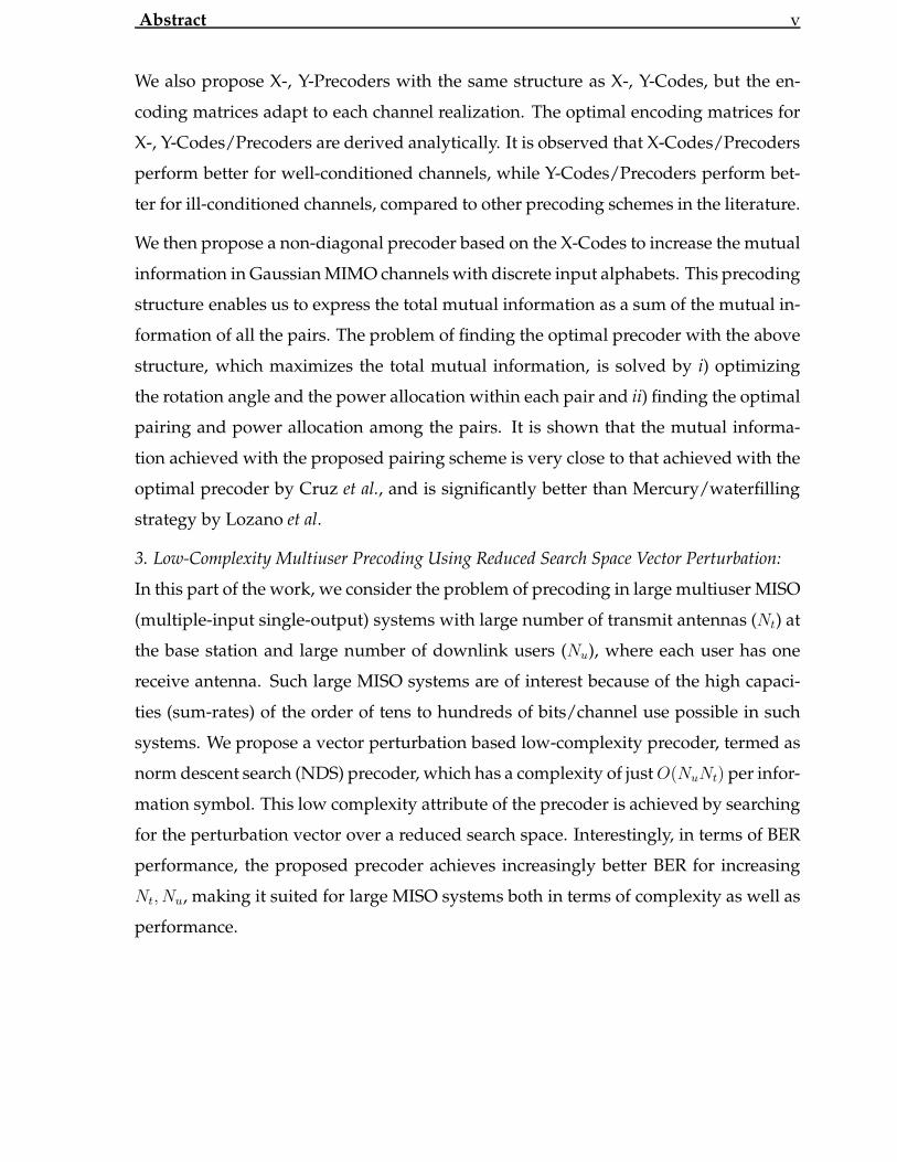
3. Low-Complexity Multiuser Precoding Using Reduced Search Space Vector Perturbation:
In this part of the work, we consider the problem of precoding in large multiuser MISO
(multiple-input single-output) systems with large number of transmit antennas (Nt) at
the base station and large number of downlink users (Nu), where each user has one
receive antenna. Such large MISO systems are of interest because of the high capaci-
ties (sum-rates) of the order of tens to hundreds of bits/channel use possible in such
systems. We propose a vector perturbation based low-complexity precoder, termed as
norm descent search (NDS) precoder, which has a complexity of just O(NuNt) per infor-
mation symbol. This low complexity attribute of the precoder is achieved by searching
for the perturbation vector over a reduced search space. Interestingly, in terms of BER
performance, the proposed precoder achieves increasingly better BER for increasing
Nt, Nu, making it suited for large MISO systems both in terms of complexity as well as
performance.

Glossary
3GPP : Third Generation Partnership ProjectASIC : Application Specific Integrated CircuitAWGN : Additive White Gaussian NoiseBC : BroadCastBER : Bit Error RateBPCU : Bits Per Channel UseBPSK : Binary Phase Shift KeyingBS : Base StationCDA : Cyclic Division AlgebraCDMA : Code Division Multiple AccessCEP/CER : Codeword Error Probability/RateCI : Channel InversionCPE : Customer Premises EquipmentCPU : Central Processing UnitCSI : Channel State InformationCSIR : CSI at the ReceiverCSIT : CSI at the TransmitterDMG : Diversity-Multiplexing GainDPC : Dirty Paper CodingDSL : Digital Subscriber LineEE : Equal EnergyFD : Full DiversityFPGA : Field Programmable Gate ArraysHDTV : High-Definition TeleVisionIC : Interference CancellationIF : Intermediate Frequencyi.i.d. : Independent and Identically DistributedILL : Information LossLessIPTV : Internet Protocol TeleVisionISI : Inter-Symbol InterferenceISIC : Iterative Soft Interference CancellationLAS : Likelihood Ascent SearchLD : Linear DispersionLLR : Log-Likelihood RatioLOS : Line-Of-Sight
vi

Glossary vii
LTE-A : Long Term Evolution - AdvancedMAC : Media Access ControlMAP : Maximum a PosterioriMF : Matched FilterMIMO : Multiple-Input Multiple-OutputMISO : Multiple-Input Single-OutputML : Maximum LikelihoodMLD : Maximum Likelihood DetectionM-LAS : Multistage LASMMSE : Minimum Mean Square ErrorNDS : Norm-Descent SearchNLOS : Non-LOSOFDM : Orthogonal Frequency Division MultiplexingPAM : Pulse Amplitude ModulationPDA : Probabilistic Data AssociationQAM : Quadrature Amplitude ModulationQOSTBC : Quasi-Orthogonal STBCQPSK : Quadrature Phase Shift KeyingRF : Radio FrequencySD : Sphere DecoderSE : Sphere EncoderSER : Symbol Error RateSIC : Successive Interference CancellationSIMO : Single-Input Multiple-OutputSINR : Signal-to-Interference plus Noise RatioSISO : Single-Input Single-OutputSNR : Signal-to-Noise RatioSTBC : Space-Time Block CodeSVD : Singular Value DecompositionTDD : Time Division DuplexingTHP : Tomlinson-Harashima PrecodingUWB : Ultra WideBandV-BLAST : Vertical Bell Lab Space-Time architectureVP : Vector PerturbationWEP : Word Error ProbabilityWiMAX : Worldwide Interoperability for Microwave AccessWLAN : Wireless Local Area NetworkWPAN : Wireless Personal Area NetworkZF : Zero Forcing
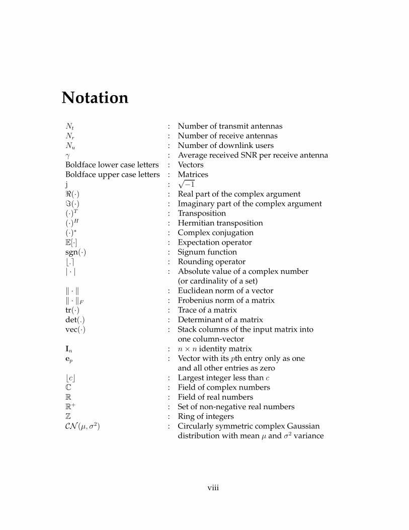
Notation
Nt : Number of transmit antennasNr : Number of receive antennasNu : Number of downlink usersγ : Average received SNR per receive antennaBoldface lower case letters : VectorsBoldface upper case letters : Matricesj :
√−1
<(·) : Real part of the complex argument=(·) : Imaginary part of the complex argument(·)T : Transposition(·)H : Hermitian transposition(·)∗ : Complex conjugationE[·] : Expectation operatorsgn(·) : Signum functionb.e : Rounding operator| · | : Absolute value of a complex number
(or cardinality of a set)‖ · ‖ : Euclidean norm of a vector‖ · ‖F : Frobenius norm of a matrixtr(·) : Trace of a matrixdet(.) : Determinant of a matrixvec(·) : Stack columns of the input matrix into
one column-vectorIn : n× n identity matrixep : Vector with its pth entry only as one
and all other entries as zerobcc : Largest integer less than cC : Field of complex numbersR : Field of real numbersR+ : Set of non-negative real numbersZ : Ring of integersCN (µ, σ2) : Circularly symmetric complex Gaussian
distribution with mean µ and σ2 variance
viii

Contents
Acknowledgments i
Abstract iii
Glossary vi
Notation viii
1 Introduction 1
1.1 Multi-Antenna Wireless Channels . . . . . . . . . . . . . . . . . . . . . . 1
1.2 MIMO System Model . . . . . . . . . . . . . . . . . . . . . . . . . . . . . . 3
1.3 MIMO Communication with CSIR Only . . . . . . . . . . . . . . . . . . . 5
1.3.1 Slow Fading Channels . . . . . . . . . . . . . . . . . . . . . . . . . 6
1.3.2 Fast Fading Channels . . . . . . . . . . . . . . . . . . . . . . . . . 7
1.4 MIMO Communication with CSIT and CSIR . . . . . . . . . . . . . . . . 9
1.5 Multiuser MIMO Communication . . . . . . . . . . . . . . . . . . . . . . 11
1.6 Challenges in Realizing Large-MIMO Systems . . . . . . . . . . . . . . . 13
1.6.1 Availability of Large Number of Independent Spatial Dimensions 14
1.6.2 Placement of Large Number of Antennas . . . . . . . . . . . . . . 14
1.6.3 Low-Complexity Detection/Channel Estimation . . . . . . . . . . 16
1.7 Problems Addressed and Contributions Made . . . . . . . . . . . . . . . 18
1.7.1 Low-Complexity Large-MIMO Detection/Channel Estimation . 19
1.7.2 Low-Complexity Large-MIMO Precoding Using X-, Y-Codes . . . 23
1.7.3 Low-Complexity Large Multiuser MISO Precoding . . . . . . . . 26
1.8 Organization of the Thesis . . . . . . . . . . . . . . . . . . . . . . . . . . . 26
ix

CONTENTS x
2 Large-MIMO Detection Using Likelihood Ascent Search 28
2.1 System Model . . . . . . . . . . . . . . . . . . . . . . . . . . . . . . . . . . 29
2.1.1 V-BLAST MIMO . . . . . . . . . . . . . . . . . . . . . . . . . . . . 29
2.1.2 Non-Orthogonal STBC MIMO . . . . . . . . . . . . . . . . . . . . 30
2.1.3 High-rate Non-orthogonal STBCs from CDA . . . . . . . . . . . . 33
2.1.4 Unified System Model . . . . . . . . . . . . . . . . . . . . . . . . . 34
2.1.5 Maximum-Likelihood Detector . . . . . . . . . . . . . . . . . . . . 35
2.2 Proposed Multistage LAS Detector . . . . . . . . . . . . . . . . . . . . . . 36
2.2.1 One-symbol Update . . . . . . . . . . . . . . . . . . . . . . . . . . 37
2.2.2 Why Multiple Symbol Updates? . . . . . . . . . . . . . . . . . . . 40
2.2.3 K-symbol Update . . . . . . . . . . . . . . . . . . . . . . . . . . . 40
2.2.4 Computational Complexity of the M-LAS Algorithm . . . . . . . 43
2.2.5 Generation of Soft Outputs . . . . . . . . . . . . . . . . . . . . . . 47
2.3 Performance in Large V-BLAST MIMO . . . . . . . . . . . . . . . . . . . . 49
2.4 Performance in Large Non-orthogonal STBC MIMO . . . . . . . . . . . . 53
2.4.1 Uncoded BER as a Function of Increasing Nt = Nr . . . . . . . . . 54
2.4.2 Performance of FD-ILL versus ILL-only STBCs . . . . . . . . . . . 55
2.4.3 Decoding and BER of Perfect Codes of Large Dimensions . . . . 56
2.4.4 Comparison with Other Large-MIMO Architecture/Detector
Combinations . . . . . . . . . . . . . . . . . . . . . . . . . . . . . . 58
2.4.5 Turbo Coded BER and Nearness-to-Capacity Results . . . . . . . 62
2.4.6 Effect of MIMO Spatial Correlation . . . . . . . . . . . . . . . . . . 65
2.5 Iterative Detection/Channel Estimation . . . . . . . . . . . . . . . . . . . 69
2.5.1 MMSE Estimation Scheme . . . . . . . . . . . . . . . . . . . . . . . 71
2.5.2 Proposed Iterative Detection/Estimation Scheme . . . . . . . . . 71
2.5.3 BER Performance with Estimated CSIR . . . . . . . . . . . . . . . 72
2.5.4 On Optimum Nt for a Given Nr and T . . . . . . . . . . . . . . . . 78
3 Large-System Performance Analysis of LAS Algorithm 80
3.1 Asymptotic Analysis of the LAS Algorithm . . . . . . . . . . . . . . . . . 81
3.2 Simulation Results and Discussions . . . . . . . . . . . . . . . . . . . . . 92
CONTENTS xi
4 Large-MIMO Detection Using Probabilistic Data Association 96
4.1 System Model . . . . . . . . . . . . . . . . . . . . . . . . . . . . . . . . . . 96
4.2 Proposed PDA Based Detection . . . . . . . . . . . . . . . . . . . . . . . . 97
4.2.1 Iterative Procedure . . . . . . . . . . . . . . . . . . . . . . . . . . . 98
4.2.2 Complexity Reduction . . . . . . . . . . . . . . . . . . . . . . . . . 101
4.3 Results and Discussions . . . . . . . . . . . . . . . . . . . . . . . . . . . . 104
4.3.1 BER Performance in Large V-BLAST MIMO . . . . . . . . . . . . 104
4.3.2 BER Performance in Large STBC MIMO . . . . . . . . . . . . . . 105
5 Large-MIMO Precoding Using X- and Y-Codes 110
5.1 System Model and SVD Precoding . . . . . . . . . . . . . . . . . . . . . . 111
5.2 Pairing Good and Bad Subchannels . . . . . . . . . . . . . . . . . . . . . . 113
5.2.1 ML Decoding . . . . . . . . . . . . . . . . . . . . . . . . . . . . . . 115
5.2.2 Performance Analysis . . . . . . . . . . . . . . . . . . . . . . . . . 117
5.2.3 Design of Optimal Pairing . . . . . . . . . . . . . . . . . . . . . . . 119
5.3 X-Codes and X-Precoder . . . . . . . . . . . . . . . . . . . . . . . . . . . . 120
5.3.1 X-Codes and X-Precoders: Encoding . . . . . . . . . . . . . . . . . 120
5.3.2 X-Codes and X-Precoders: ML Decoding . . . . . . . . . . . . . . 121
5.3.3 Optimal Design of X-Codes . . . . . . . . . . . . . . . . . . . . . . 121
5.3.4 Optimal Design of X-Precoder . . . . . . . . . . . . . . . . . . . . 125
5.4 Y-Codes and Y-Precoder . . . . . . . . . . . . . . . . . . . . . . . . . . . . 127
5.4.1 Motivation . . . . . . . . . . . . . . . . . . . . . . . . . . . . . . . . 127
5.4.2 Y-Codes and Y-Precoders: Encoding . . . . . . . . . . . . . . . . . 128
5.4.3 Y-Codes and Y-Precoders: ML Decoding . . . . . . . . . . . . . . 129
5.4.4 Optimal Design of Y-Codes . . . . . . . . . . . . . . . . . . . . . . 131
5.4.5 Optimal Design of Y-Precoder . . . . . . . . . . . . . . . . . . . . 133
5.5 Simulation Results . . . . . . . . . . . . . . . . . . . . . . . . . . . . . . . 135
5.5.1 Effect of Channel Condition on Error Performance . . . . . . . . . 135
5.5.2 Diversity Order Comparison . . . . . . . . . . . . . . . . . . . . . 137
5.5.3 Comparison of BER Performance with Full-rate Transmission . . 137
5.5.4 Comparison of BER Performance for Nt = Nr = 2, 4 . . . . . . . . 138
5.5.5 Comparison of BER Performance for Nt = Nr = 16 . . . . . . . . 140
CONTENTS xii
5.5.6 X-Codes versus Y-Codes . . . . . . . . . . . . . . . . . . . . . . . . 140
5.5.7 X-, Y-Codes versus X-, Y-Precoders . . . . . . . . . . . . . . . . . . 141
5.6 Complexity . . . . . . . . . . . . . . . . . . . . . . . . . . . . . . . . . . . . 144
5.6.1 Encoding Complexity . . . . . . . . . . . . . . . . . . . . . . . . . 145
5.6.2 Decoding Complexity . . . . . . . . . . . . . . . . . . . . . . . . . 145
6 Precoding with X-codes to Increase Capacity with Discrete Input Alphabets 147
6.1 System Model and Precoding with Gaussian Inputs . . . . . . . . . . . . 149
6.2 Optimal Precoding with Discrete Inputs . . . . . . . . . . . . . . . . . . . 151
6.3 Precoding with X-Codes . . . . . . . . . . . . . . . . . . . . . . . . . . . . 152
6.4 Gaussian MIMO Channels with n = 2 . . . . . . . . . . . . . . . . . . . . 156
6.5 Gaussian MIMO Channels with n > 2 . . . . . . . . . . . . . . . . . . . . 164
6.6 Application to OFDM and Large-MIMO . . . . . . . . . . . . . . . . . . . 167
7 NDS Precoder for Large Multiuser MISO Systems 173
7.1 System Model . . . . . . . . . . . . . . . . . . . . . . . . . . . . . . . . . . 174
7.1.1 Vector Perturbation . . . . . . . . . . . . . . . . . . . . . . . . . . . 176
7.2 Proposed NDS Precoder . . . . . . . . . . . . . . . . . . . . . . . . . . . . 178
7.2.1 Complexity of the NDS Algorithm . . . . . . . . . . . . . . . . . . 182
7.3 Results and Discussions . . . . . . . . . . . . . . . . . . . . . . . . . . . . 183
7.3.1 NDS-MMSE versus NDS-ZF Precoder Performance . . . . . . . . 183
7.3.2 NDS-MMSE versus MMSE-only and VP-SE Schemes . . . . . . . 185
7.3.3 Nearness to Sum Capacity . . . . . . . . . . . . . . . . . . . . . . 187
8 Conclusions 192
A Proof of Optimum Update l(k)p , Chapter 2 196
B Proof of Lemma 5, Chapter 3 198
C Conjecture 1, Chapter 3 200
D Proof of Theorem 1, Chapter 5 208
E Proof of Theorem 2, Chapter 5 211

CONTENTS xiii
F Proof of Theorem 3, Chapter 5 214
List of Publications from this Thesis 216
Bibliography 218
List of Figures
1.1 MIMO System. . . . . . . . . . . . . . . . . . . . . . . . . . . . . . . . . . 4
1.2 Ergodic MIMO capacity for increasing Nt = Nr with i) CSIR only and
ii) CSIT and CSIR. . . . . . . . . . . . . . . . . . . . . . . . . . . . . . . . . 8
1.3 16-antenna indoor channel sounding measurement setup in [47]. Photos
Source: [47]. . . . . . . . . . . . . . . . . . . . . . . . . . . . . . . . . . . . 16
1.4 64×64 MIMO indoor channel sounding setup at 5 GHz reported in [48].
Photos Source: [48]. . . . . . . . . . . . . . . . . . . . . . . . . . . . . . . . 17
2.1 Mean number of stages for the 3-LAS algorithm with MMSE initial vec-
tor. V-BLAST MIMO, 4-QAM, SNR = 6, 9, 12 dB. . . . . . . . . . . . . . . 44
2.2 Mean number of iterations per stage per transmit antenna for the 3-LAS
algorithm with MMSE initial vector. V-BLAST MIMO, 4-QAM, SNR =
6, 9, 12 dB. . . . . . . . . . . . . . . . . . . . . . . . . . . . . . . . . . . . . 45
2.3 Computational complexity of the M-LAS algorithm in decoding non-
orthogonal STBCs from CDA. MMSE initial vector, 4-QAM, SNR = 6 dB. 47
2.4 Uncoded BER performance of 3-LAS detection for different values of
Nt = Nr = (16, 32, 64, 128, 256) and 4-QAM. MMSE initial filter. . . . . . . 50
2.5 Average received SNR required to achieve a target BER of 10−3 in V-
BLAST MIMO for increasing values of Nt = Nr using 1-LAS detection
with MMSE initial vector. 4-QAM. . . . . . . . . . . . . . . . . . . . . . . 51
2.6 Average received SNR required to achieve a target BER of 10−4 in V-
BLAST MIMO for increasing values of Nt = Nr using 1-LAS detection
with MMSE initial vector. 16-QAM. . . . . . . . . . . . . . . . . . . . . . 51
xiv
LIST OF FIGURES xv
2.7 Comparison of 3-LAS and 1-LAS performance in V-BLAST MIMO for
Nt = Nr = 64, 32 and 4-QAM. MMSE initial vector. . . . . . . . . . . . . . 52
2.8 Turbo coded BER performance of 3-LAS detection for Nt = Nr = 64, 128,
4-QAM, and rate-3/4 turbo code. MMSE initial vector. . . . . . . . . . . 53
2.9 Uncoded BER performance of 1-LAS, 2-LAS and 3-LAS detectors for
ILL-only STBCs for different Nt = Nr. 4-QAM, 2Nt bps/Hz. . . . . . . . 54
2.10 Uncoded BER performance comparison between FD-ILL and ILL-only
STBCs for different Nt = Nr. 4-QAM, 2Nt bps/Hz, 1-LAS detection
with MMSE initial vector. . . . . . . . . . . . . . . . . . . . . . . . . . . . 55
2.11 Uncoded BER comparison between perfect codes and ILL-only STBCs
for different Nt = Nr, 4-QAM, 2Nt bps/Hz, 1-LAS detection. . . . . . . 57
2.12 Uncoded BER performance comparison between perfect codes, ILL-only,
and FD-ILL STBCs for Nt = Nr = 16, 32, 16-QAM, 4Nt bps/Hz, 1-LAS
detection. . . . . . . . . . . . . . . . . . . . . . . . . . . . . . . . . . . . . . 58
2.13 Uncoded BER performance comparison between the 1-LAS algorithm
and the ISIC algorithm in [111] for ILL-only STBCs for different Nt = Nr.
4-QAM, 2Nt bps/Hz. MMSE initial vectors for both 1-LAS and ISIC. . . 59
2.14 Uncoded BER comparison between different large-MIMO architecture/detector
combinations for given number of transmit/receive antennas (Nt = Nr =
16) and spectral efficiency (32 bps/Hz). . . . . . . . . . . . . . . . . . . . 60
2.15 Turbo coded BER performance of 1-LAS detector for 16×16 FD-ILL and
ILL-only STBCs. Nt = Nr = 16, 4-QAM, turbo code rates: 1/3, 1/2, 3/4
(10.6, 16, 24 bps/Hz). . . . . . . . . . . . . . . . . . . . . . . . . . . . . . . 63
2.16 Turbo coded BER performance of 1-LAS detector for 32 × 32 ILL-only
STBC. Nt = Nr = 32, 16-QAM, turbo code rates: 1/3, 1/2, 3/4 (42.6, 64,
96 bps/Hz). . . . . . . . . . . . . . . . . . . . . . . . . . . . . . . . . . . . 64
2.17 Turbo codeword error probability of 1-LAS detection in a slow fading
MIMO channel for Nt = Nr = 4, 8, 12, 4-QAM, rate-3/4 turbo code and
FD-ILL STBCs. MMSE initial vector. . . . . . . . . . . . . . . . . . . . . . 64
2.18 Propagation scenario for the MIMO fading channel model. . . . . . . . . 67

LIST OF FIGURES xvi
2.19 Effect of Nr > Nt in correlated MIMO fading channel model in [8] keep-
ing Nrdr constant and dt = dr. Nrdr = 72 cm, fc = 5 GHz, R = 500 m,
S = 30, Dt = Dr = 20 m, θt = θr = 90◦, 12× 12 ILL-only STBC, Nt = 12,
Nr = 12, 18, 16-QAM, rate-3/4 turbo code, 36 bps/Hz. . . . . . . . . . . . 68
2.20 Transmission scheme with one pilot matrix followed by Nd data STBC
matrices in each frame. . . . . . . . . . . . . . . . . . . . . . . . . . . . . . 71
2.21 Hassibi-Hochwald (H-H) capacity bound for 1P+8D (T = 144, τ = 16, βp =
βd = 1) and 1P+1D (T = 32, τ = 16, βp = βd = 1) training for a 16 × 16
MIMO channel. Perfect CSIR capacity is also shown. . . . . . . . . . . . . 73
2.22 Uncoded BER of 1-LAS detector for 16×16 ILL-only STBC with i) perfect
CSIR, ii) CSIR using MMSE estimation scheme, and iii) CSIR using iter-
ative detection/channel estimation scheme (4 iterations). Nt = Nr = 16,
4-QAM, 1P+1D(T = 32, τ = 16, βp = βd = 1
)and 1P+8D
(T = 144, τ =
16, βp = βd = 1)
training. . . . . . . . . . . . . . . . . . . . . . . . . . . . 74
2.23 Turbo coded BER performance of 1-LAS detector for 16 × 16 ILL-only
STBC with i) perfect CSIR, ii) CSIR using MMSE estimation, and iii)
CSIR using iterative detection/channel estimation (4 iterations). Nt =
Nr = 16, 4-QAM, rate-3/4 turbo code, 1P+1D(T = 32, τ = 16, βp = βd =
1)
and 1P+8D(T = 144, τ = 16, βp = βd = 1
)training. . . . . . . . . . . . 75
2.24 Turbo coded BER performance of 1-LAS detection and iterative estima-
tion/detection as a function of coherence time, T = 32, 144, 400, 784, for
a given Nt = Nr = 16, 16 × 16 ILL-only STBC, 4-QAM, rate-3/4 turbo
code. . . . . . . . . . . . . . . . . . . . . . . . . . . . . . . . . . . . . . . . 76
2.25 Comparison between two 1P+NdD training-based systems, one with a
larger Nt than the other for a given Nr and T . . . . . . . . . . . . . . . . 77
3.1 Simulated pdf of zun,d for n = 2Nt for increasing Nt = Nr. 4-QAM. The
pdf tends towards Dirac delta function at zero. . . . . . . . . . . . . . . . 85
3.2 Conditional probabilities pr,r+1 as a function of increasing Nt = Nr for
the 1-LAS detector with MMSE initial vector. 4-QAM and SNR = 10 dB. 87
3.3 Conditional probabilities pr,r+1 as a function of increasing Nt = Nr for
the 1-LAS detector with Random initial vector. 4-QAM and SNR = 10 dB. 88

LIST OF FIGURES xvii
3.4 Simulated BER performance of the 1-LAS detector for V-BLAST MIMO
as a function of average received SNR for increasing values of Nt = Nr.
MMSE initial vector, 4-QAM. . . . . . . . . . . . . . . . . . . . . . . . . . 92
3.5 Simulated BER performance of 1-LAS detector with Random initial vec-
tor for increasing Nt = Nr. 4-QAM. . . . . . . . . . . . . . . . . . . . . . . 93
3.6 Simulated BER performance of the 1-LAS detector with MF initial vector
for increasing Nt = Nr. 4-QAM. . . . . . . . . . . . . . . . . . . . . . . . . 93
3.7 BER performance comparison between Random 1-LAS and Random 3-
LAS detectors for increasing Nt = Nr. 4-QAM. . . . . . . . . . . . . . . . 94
4.1 BER performance of PDA based detection in a V-BLAST MIMO system
with Nt = Nr = 64 and 4-QAM for different number of PDA iterations
(m = 1, 2, 4, 8). . . . . . . . . . . . . . . . . . . . . . . . . . . . . . . . . . . 104
4.2 BER performance of PDA based detection of V-BLAST MIMO for Nt =
Nr = 8, 16, 32, 64, 96, 4-QAM, and m = 5 iterations. . . . . . . . . . . . . 105
4.3 Comparison between the uncoded BER performance of PDA and LAS
algorithms in decoding 4 × 4, 8 × 8, 16 × 16 ILL-only STBCs. Nt = Nr,
4-QAM, m = 10. . . . . . . . . . . . . . . . . . . . . . . . . . . . . . . . . . 106
4.4 Comparison between the uncoded BER performance of PDA and LAS
algorithms in decoding 4 × 4, 8 × 8, 16 × 16 ILL-only STBCs. Nt = Nr,
16-QAM. . . . . . . . . . . . . . . . . . . . . . . . . . . . . . . . . . . . . . 107
4.5 Turbo coded BER performance of the PDA algorithm in decoding 12×12
ILL-only STBC with Nt = Nr = 12, 4-QAM, rate-3/4 turbo code, 18
bps/Hz and m = 10 for i) perfect CSIR, and ii) estimated CSIR using 2
iterations between PDA decoding/channel estimation. . . . . . . . . . . 107
4.6 Effect of spatial correlation on the performance of PDA in decoding 12×12 ILL STBC from CDA. Nt = 12, Nr = 12, 18, 16-QAM, rate-3/4 turbo
code, 36 bps/Hz. Correlated channel parameters: fc = 5 GHz, R = 500
m, S = 30, Dt = Dr = 20 m, θt = θr = 90◦, Nrdr = 72 cm, dt = dr. . . . . . 109
5.1 Union bound for the word error probability. Nt = Nr = 2 and M = 2
(4-QAM). . . . . . . . . . . . . . . . . . . . . . . . . . . . . . . . . . . . . . 123
LIST OF FIGURES xviii
5.2 Sensitivity of word error probability w.r.t. θ1. Nr = Nt = 2 and M = 2, 4
(4-QAM, 16-QAM). . . . . . . . . . . . . . . . . . . . . . . . . . . . . . . . 124
5.3 One quadrant of the set SM for M = 2, 4 (4-QAM, 16-QAM). The critical
angles where performance degrades severely are shown to coincide with
tan−1(−p/q). . . . . . . . . . . . . . . . . . . . . . . . . . . . . . . . . . . . 125
5.4 Received signal space for the real component of the kth pair. M = 8 and
so we have 5 regions with vertical dashed lines demarcating the bound-
ary between the regions. The scaled codebook vectors are represented
by small filled circles along with their corresponding codebook index
number. Dotted lines demarcate the boundary between the ML decision
regions. . . . . . . . . . . . . . . . . . . . . . . . . . . . . . . . . . . . . . . 131
5.5 Effect of the channel condition number on error performance of various
precoders for a 2 × 2 system with target spectral efficiency equal to 8
bps/Hz. . . . . . . . . . . . . . . . . . . . . . . . . . . . . . . . . . . . . . 136
5.6 BER comparison between various precoders for Nt = Nr = Ns = 2, 4
and M = 2 (4-QAM). Target spectral efficiency is equal to 2Ns bps/Hz. . 138
5.7 BER comparison between various precoders for Nt = Nr = 2 and target
spectral efficiency = 4, 8 bps/Hz. . . . . . . . . . . . . . . . . . . . . . . . 139
5.8 BER comparison between various precoders for Nt = Nr = 4 and target
spectral efficiency = 8, 16 bps/Hz. . . . . . . . . . . . . . . . . . . . . . . 139
5.9 BER comparison between various precoders for Nt = Nr = 16 and target
spectral efficiency = 64 bps/Hz. . . . . . . . . . . . . . . . . . . . . . . . . 141
5.10 BER comparison between the proposed X-Codes and Y-Codes for Nt =
Nr = 2 with spectral efficiency = 4, 8 bps/Hz. . . . . . . . . . . . . . . . . 142
5.11 BER comparison between the proposed X-Codes and Y-Codes for Nt =
Nr = 4 with spectral efficiency = 8, 16 bps/Hz. . . . . . . . . . . . . . . . 142
5.12 Word error probability comparison between the proposed suboptimal
Y-Precoders and exact optimal Y-Precoders for Nt = Nr = 2, 4 with spec-
tral efficiency = 4Nt bps/Hz. . . . . . . . . . . . . . . . . . . . . . . . . . . 144
6.1 Plot of f opt versus PT for n = 2 parallel channels with β = 1, 1.5, 2, 4, 8
and α = 1. Input alphabet is 16-QAM. . . . . . . . . . . . . . . . . . . . . 158
LIST OF FIGURES xix
6.2 Plot of θopt versus PT for n = 2 parallel channels with β = 1.5, 2, 4, 8 and
α = 1. Input alphabet is 16-QAM. . . . . . . . . . . . . . . . . . . . . . . . 158
6.3 Mutual Information of X-Codes versus power allocation fraction f for
n = 2 parallel channels with β = 1, 1.5, 2, 4, 8, α = 1 and PT = 17 dB.
Input alphabet is 16-QAM. . . . . . . . . . . . . . . . . . . . . . . . . . . . 159
6.4 Mutual information of X-Codes versus rotation angle θ for n = 2 parallel
channels with β = 1, 1.5, 2, 4, 8, α = 1 and PT = 17 dB. Input alphabet is
16-QAM. . . . . . . . . . . . . . . . . . . . . . . . . . . . . . . . . . . . . . 160
6.5 Mutual information versus PT for X-Codes for different θ’s, n = 2 paral-
lel channels, α = 1, β = 2, and 4-QAM input alphabet. . . . . . . . . . . 160
6.6 Mutual information versus PT for n = 2 parallel channels with β = 2
and α = 1, for 4-QAM and 16-QAM. . . . . . . . . . . . . . . . . . . . . . 161
6.7 Mutual information versus PT for n = 2 parallel channels with varying
β = 1, 2, 4, α = 1 and 4-QAM input alphabet. . . . . . . . . . . . . . . . . 162
6.8 Mutual information with X-Codes versus PT for n = 2 parallel channels
with varying β = 1, 1.5, 2, 4, 8, α = 1 and 16-QAM input alphabet. . . . . 164
6.9 Mutual information versus PT with two different pairings for a n = 4
diagonal channel and 16-QAM input alphabet. . . . . . . . . . . . . . . . 165
6.10 Mutual information versus PT for the Gigabit DSL channel given by (42)
in [95]. . . . . . . . . . . . . . . . . . . . . . . . . . . . . . . . . . . . . . . 165
6.11 Comparison of 4×4 wireless MIMO ergodic capacity with perfect CSIT/CSIR
for 16-QAM input alphabet. . . . . . . . . . . . . . . . . . . . . . . . . . . 166
6.12 Mutual information versus per subcarrier SNR for an OFDM system
with 32 carriers. X-Codes versus Mercury/waterfilling. . . . . . . . . . . 169
6.13 Mutual information versus per subcarrier SNR for a OFDM system with
32 carriers. Comparison of heuristic pairing schemes. . . . . . . . . . . . 170
6.14 Comparison of 16 × 16 wireless MIMO ergodic capacity with perfect
CSIT/CSIR for 16-QAM input alphabet. . . . . . . . . . . . . . . . . . . . 172
7.1 Multiuser MISO system on the downlink. . . . . . . . . . . . . . . . . . . 174
7.2 Proposed norm-descent search precoder. . . . . . . . . . . . . . . . . . . . 179
LIST OF FIGURES xx
7.3 Average number of iterations per information symbol till the NDS algo-
rithm terminates as a function of (Nt, Nu). Nt = Nu, Nr = 1, 4-QAM,
GMMSE precoding matrix. . . . . . . . . . . . . . . . . . . . . . . . . . . . . 183
7.4 Uncoded BER performance of the proposed NDS-MMSE and NDS-ZF
precoders for Nt = Nu = 10, 50, 200. Nr = 1, 4-QAM. . . . . . . . . . . . 184
7.5 Uncoded BER performance comparison of the proposed NDS-MMSE
precoder versus i) MMSE-only precoder, and ii) the VP-SE scheme. Nu =
8 and Nt = 8, 16, Nr = 1, 4-QAM. . . . . . . . . . . . . . . . . . . . . . . . 185
7.6 Complexity of the proposed NDS-MMSE precoder in comparison with
that of the VP-SE scheme. Nt = Nu, Nr = 1, 4-QAM, SNR = 15 dB. . . . . 187
7.7 Upper and lower bounds for the ergodic sum capacity, Csum. . . . . . . . 189
7.8 Turbo coded BER performance comparison between the NDS-MMSE
and VP-SE schemes for Nu = 8, Nt = 8, 12, 16, Nr = 1, 4-QAM, rate-
3/4 turbo code, sum rate = 12 bps/Hz. . . . . . . . . . . . . . . . . . . . . 190
7.9 Turbo coded BER performance of the proposed NDS-MMSE precoder
without and with channel estimation errors. Nt = Nu = 300, Nr = 1,
4-QAM, rate-3/4 turbo code, sum rate = 450 bps/Hz. . . . . . . . . . . . 191

List of Tables
2.1 Complexity and performance comparison of different large-MIMO ar-
chitecture/detector combinations, all with Nt = Nr = 16 and achieving
32 bps/Hz spectral efficiency. . . . . . . . . . . . . . . . . . . . . . . . . . 61
2.2 On optimum Nt for a given Nr and T . System-II with a smaller Nt
achieves a higher spectral efficiency while achieving 10−3 coded BER
at a lesser SNR than System-I with a larger Nt. . . . . . . . . . . . . . . . 78
4.1 Listing of the proposed PDA based detection algorithm. . . . . . . . . . 103
7.1 Listing of the proposed NDS precoding algorithm. . . . . . . . . . . . . . 182
xxi
Chapter 1
Introduction
Multiple-input multiple-output (MIMO) systems with multiple antennas at the trans-
mitter and receiver sides have become very popular owing to the several advantages
they promise to offer, including high data rates and transmit diversity [1]-[4]. For ex-
ample, current wireless standards including WiFi (IEEE 802.11n) and WiMAX (IEEE
802.16e) and 3GPP LTE-A have adopted MIMO techniques in their physical layer. It
is known that the capacity of MIMO channels grows linearly with the minimum of
the number of antennas on the transmitter and receiver sides [5],[6], which motivates
the use of large number of antennas at the communication terminals to achieve high
spectral efficiencies as well as high diversity orders in wireless transmissions.
1.1 Multi-Antenna Wireless Channels
Multi-antenna wireless channels are a broad category of channels that include point-
to-point and multiuser channels (e.g., MAC, broadcast, and relay channels, to name
a few). One of the defining characteristics of a wireless channel is the variation of
the channel strength over time and over frequency [4],[7]. These variations are typi-
cally classified into two types: large-scale fading and small-scale fading. Large-scale
fading is due to path loss of the signal as a function of distance and shadowing by
1
Chapter 1. Introduction 2
large objects like buildings, bridges and trees, and is typically frequency independent.
Small-scale fading, on the other hand, is due to the constructive and destructive inter-
ference of the multiple signal paths between the transmitter and receiver. Small-scale
fading happens at the spatial scale of the order of the carrier wavelength, and is fre-
quency dependent which makes the channel to be classified as frequency-selective or
frequency-flat. When the signaling bandwidth is larger than the coherence bandwidth
of the channel (which has an inverse relation with the maximum delay spread of the
channel), the channel is frequency-selective. In frequency-flat channels, the signal-
ing bandwidth is much smaller than the coherence bandwidth of the channel [7]. In
this thesis, we will consider the channel to be frequency-flat. Even when the chan-
nel is frequency-selective, techniques like orthogonal frequency division multiplexing
(OFDM) can convert the channel into multiple frequency-flat channels on which the
techniques proposed in this thesis can be employed. In terms of time variation, wire-
less channels are further classified as slowly fading or fast fading, depending on the
fade rate relative to the signaling rate. If the fade remains constant over the signal-
ing duration, the fading is termed as slow (or time-flat) fading, whereas if the fade
varies within the signaling duration, it is termed as fast (or time-selective) fading. Car-
rier wavelength and velocity of the communication terminal determine the amount of
time-selectivity (or Doppler spread) in the channel [7].
Most multi-antenna wireless channels with Nr receive and Nt transmit antennas (e.g.,
see Fig. 1.1) are modeled as a linear channel with an equivalent baseband channel ma-
trix Hc ∈ CNr×Nt . The (i, j)th entry of Hc, i.e., hi,j represents the channel gain from the
jth transmit antenna to the ith receive antenna. These channel gains can be indepen-
dent or correlated, which depends upon various factors, including spacing between
transmit and receive antennas, amount of scattering in the environment, pin-hole ef-
fects, etc. [8]. Mathematical models that characterize the spatial correlation in MIMO
channels are used in the performance evaluation of MIMO systems. Spatial correlation
Chapter 1. Introduction 3
at the transmit and/or receive side can affect the rank structure of the MIMO channel
resulting in degraded MIMO capacity [9]. The structure of scattering in the propaga-
tion environment can also affect the capacity [8]. Also, transmit correlation in MIMO
fading can be exploited by using non-isotropic inputs (precoding) based on the knowl-
edge of the channel correlation matrices [10]-[12].
The channel gains are also referred to as the channel state information (CSI). Availability
of the knowledge of these gains at the receiver and transmitter is an important fac-
tor which decides the performance of the communication system. CSI at the receiver
(CSIR) refers to the scenario where the receiver has the knowledge of the channel gains.
Likewise, CSI at the transmitter (CSIT) refers to the scenario where the transmitter has
the knowledge of the channel gains. In fast fading channels, accurate estimation of the
channel gains can become an issue, in which case non-coherent or blind techniques
can be considered. In addition, feedback based provision of CSIT can become inef-
fective in fast fading. However, in applications where the channel is not varying fast,
it is generally possible to estimate the channel gains accurately through pilot-assisted
transmission. Also, CSIT based on feedback from measured CSI from the receiver is
effective in such slow fading channels.
1.2 MIMO System Model
Assuming frequency-flat and slow fading, where the channel gains are assumed to
remain constant over the signaling interval, the equivalent complex baseband MIMO
system model can be written as
yc = Hcxc + nc, (1.1)
where xc ∈ CNt is the transmitted vector, yc ∈ CNr is the received vector, and nc ∈ CNr
is the additive white Gaussian noise (AWGN) vector. The jth entry of xc is the symbol

Chapter 1. Introduction 4
Detector
EstimatedData
MIMO Channel
Input Data Stream
Encoder
Tx−1
Tx−2
Tx− Rx−
Rx−2
Rx−1
MIMOMIMO
NrNt
Nt Nr : # Transmit Antennas : # Receive Antennas
Figure 1.1: MIMO System.
transmitted from the jth transmit antenna, j = 1, · · · , Nt. In a typical communica-
tion system, information bits (e.g., output of some source coder, like image or voice
compression, followed by a channel coder) are grouped into messages, and each mes-
sage then corresponds to an Nt-dimensional complex vector, whose jth component is
transmitted from the jth transmit antenna. In practice, these vectors belong to some
codebook X . The transmitter groups R = log2 |X | bits into a message, which is then
used to index into the codebook. R is often referred to as the rate of the codebook or
simply as the rate of transmission. Alternatively, the xc vector could be a pilot symbol
vector (known to the receiver) during the training phase in a pilot-aided channel es-
timation scheme. The ith entry of yc is the signal received at the ith receive antenna,
i = 1, · · · , Nr. Assuming a rich scattering environment, the entries of the channel ma-
trix Hc are often modeled as i.i.d. (independent and identically distributed) CN (0, 1).
Since the transmitter is power constrained, we have E[tr(xcxHc )] = P , where P is the
total power available at the transmitter. Also, E[ncnHc ] = σ2INr , where σ2 is the noise
variance at each receive antenna. The average received signal-to-noise ratio (SNR) at
each receive antenna is given by γ = Pσ2 .

Chapter 1. Introduction 5
The MIMO signal detection problem can be stated as: Given yc and the knowledge
of Hc, determine xc, an estimate of the transmitted symbol vector xc. Likewise, the
MIMO channel estimation problem in a training-based scheme can be stated as: Given
the knowledge of the transmitted pilot symbol vector xc, determine Hc, an estimate of
the channel gain matrix Hc. A vast body of the MIMO literature has focused on these
two problems [13]. Joint detection/channel estimation approaches have also been in-
vestigated [14],[15]. Much of the MIMO detection and channel estimation works in the
literature so far, however, have considered only small number of antennas (e.g.,Nt =
2, 3, 4). In the first part of this thesis (Chapters 2, 3, 4), we will be concerned with MIMO
detection and channel estimation when Nt, Nr are large (e.g., tens).
1.3 MIMO Communication with CSIR Only
In communication channels, error probability is one of the key performance indicators.
Most communication schemes employ channel coding schemes to increase robustness
against errors. To achieve an arbitrarily low probability of error, the rate of transmis-
sion R must be strictly below the MIMO channel capacity. The MIMO channel capacity
is dependent on Hc and the transmit covariance matrix Kx4= E[xcx
Hc ], tr(Kx) = P , and
is given by
Cmimo(γ,Hc,Kx) = log2 det(INr +
1
σ2HcKxH
Hc
). (1.2)
In the case of availability of CSIR only, since the transmitter has no knowledge of the
channel gains, it cannot adapt its transmission scheme with respect to the channel
gains. Therefore, for a fixed γ and rate R, the transmitter uses a fixed codebook, which
does not change with changing channel gains. The transmitter codebook selection is
very much dependent on whether the channel is slow fading or fast fading.

Chapter 1. Introduction 6
1.3.1 Slow Fading Channels
In slowly fading channels, where the channel does not change during the length of
the codeword, if the channel is such that Cmimo(γ,Hc,Kx) < R, then no detector can
recover the transmitted codeword correctly, and the channel is said to be in outage.
Hence, for slow fading channels with CSIR-only, outage cannot be avoided and it is
impossible to achieve an arbitrary low probability of error. In such scenarios, an ap-
propriate performance indicator of any encoding-decoding scheme is the codeword
error probability (CEP) or codeword error rate (CER). For codewords of large length,
the theoretical limit for the codeword error rate of any encoding-decoding scheme is
the channel outage probability, which is defined as
Poutage(γ, R) = minKx |tr(Kx)=P
p(Cmimo(γ,Hc,Kx) < R
). (1.3)
Any practical encoding-decoding scheme would have a codeword error rate more than
the channel outage probability given in (1.3). Therefore, it is important to design trans-
mit schemes and corresponding receivers which can perform very close to the channel
outage probability for all values of γ and R. For slowly fading channels, there are two
important parameters, namely, diversity gain and multiplexing gain. Diversity gain is
a measure of reliability, whereas multiplexing gain is a measure of the degrees of free-
dom in the MIMO channel. These two parameters are usually related by the so called
diversity-multiplexing gain (DMG) tradeoff [16]. It is known that in Rayleigh faded
MIMO channels, the maximum diversity gain achievable is NrNt, and the maximum
multiplexing gain achievable is min(Nr, Nt). When the rate of transmission R is fixed,
the limiting value (as γ →∞) of the negative of the slope of log(Poutage(γ, R)) w.r.t. log γ
can be no more than NrNt. For a given scheme, we can therefore define the diversity
order achievable (with fixed R) as
dord = − limγ→∞
log(Pe(γ))
log γ, (1.4)

Chapter 1. Introduction 7
where Pe(γ) is the codeword error rate of the scheme. For simple MIMO schemes like
V-BLAST [17],[18], it can be shown that the maximum diversity order achievable is
only Nr. This is because symbols transmitted from the antennas are independent, and
each such symbol reaches the receiver only through Nr different paths.
Space-time block coding is a well known technique [2], which can achieve the full di-
versity gain of NrNt. To achieve full diversity, symbols are coded across both space
and time. This implies that joint detection be performed at the receiver, which makes
the receiver processing complex. Orthogonal space-time block codes (STBC) were pro-
posed as a solution to this problem [19],[20]. They, however, sacrificed on the multi-
plexing rate, and were therefore not suited for systems with high target spectral effi-
ciencies. Subsequent to orthogonal STBCs, several high-rate and high-diversity STBCs
were proposed. One such class of STBCs is non-orthogonal STBCs from Cyclic Divi-
sion Algebras (CDA) [21],[22]. STBCs from CDA can achieve the full diversity of NrNt
without sacrificing on the rate. However, due to coding across space and time, receiver
processing is challenging. The maximum-likelihood (ML) detector has a complexity
that is exponential in the number of symbols to be detected jointly. For e.g., the ML
detector for even a 4× 4 full-rate STBC from CDA with 16-QAM would have to check
the ML metric for 1616 different STBC matrices. Hence, suboptimal detectors that have
lesser complexity and can achieve near-optimal performance are of interest. Chapters
2, 3, and 4 in this thesis are concerned with low-complexity algorithms that can achieve near-
optimal performance in V-BLAST MIMO as well as non-orthogonal STBC MIMO systems
where Nt, Nr are large (e.g., tens).
1.3.2 Fast Fading Channels
In fast fading channels, the channel fade changes multiple times during the duration of
the codeword. By spreading portions of the codeword across multiple fades, reliability
of codeword reception can be improved. In such a scenario, if the MIMO channel is

Chapter 1. Introduction 8
−6 −4 −2 0 2 4 6 8 10 120
20
40
60
80
100
120
Average Received SNR (dB)
Erg
odic
Cap
acity
(bp
s/H
z)
Nr = N
t = 8, CSIR only
Nr = N
t = 8, CSIT and CSIR
Nr = N
t = 16, CSIR only
Nr = N
t = 16, CSIT and CSIR
Nr = N
t = 32, CSIR only
Nr = N
t = 32, CSIT and CSIR
Figure 1.2: Ergodic MIMO capacity for increasing Nt = Nr with i) CSIR only and ii)CSIT and CSIR.
ergodic, in the limit of infinitely long codewords, it is possible to achieve error free
communication if the rate of transmission R satisfies
R ≤ Cergodic(γ)4= max
Kx |tr(Kx)=PEHc
[Cmimo(γ,Hc,Kx)
]. (1.5)
Cergodic(γ) is often referred to as the ergodic MIMO capacity, and is achieved with Kx =
PNt
INt . This transmit architecture is also known as the V-BLAST scheme, where the
symbol streams transmitted from each transmit antenna are uncorrelated. The ergodic
MIMO capacity is therefore given by
Cergodic(γ) = EHc
[log2 det
(INr +
γ
NtHcH
Hc
)]. (1.6)
It has been shown that the ergodic MIMO capacity increases linearly with increasing
Nr = Nt [5].
In Figure 1.2, the ergodic MIMO capacity is plotted as a function of the average re-
ceived SNR, γ, for MIMO systems with CSIR-only for different values of Nt = Nr.
We observe that for a given SNR, the ergodic MIMO capacity increases linearly with

Chapter 1. Introduction 9
Nt = Nr. For e.g., at an SNR of 6.8 dB the ergodic capacity is 16, 32 and 64 bps/Hz
for Nt = Nr = 8, 16, 32, respectively. This implies that at an SNR of 6.8 dB, a Nt = Nr
MIMO system would have an ergodic capacity of roughly 2Nt bps/Hz. Hence, MIMO
systems with large Nt = Nr (which we refer to as ‘large-MIMO systems’) have the po-
tential of achieving very high spectral efficiencies of the order of tens to hundreds of
bps/Hz. However, achieving such large spectral efficiencies requires that large num-
ber of independent spatial dimensions exist. This would depend on spacing between
antennas, carrier wavelength, scattering around the wireless terminals, and spatial cor-
relation. These requirements can be favorably met in several indoor/outdoor wireless
applications with medium-/large-sized aperture communication terminals (e.g., set
top boxes, laptops, TVs, fixed nodes in wireless mesh networks). We will discuss the
technological challenges in realizing large-MIMO systems in Section 1.6.
1.4 MIMO Communication with CSIT and CSIR
If MIMO systems are operating in time division duplex (TDD) mode or if MIMO chan-
nels are slowly varying, it is possible for both the transmitter as well as the receiver
to acquire the channel state information. When both CSIT and CSIR are available, the
ergodic MIMO capacity is known to be achieved with independent Gaussian inputs
beamformed along the right singular vectors of the channel matrix. This transforms
the MIMO channel into a set of parallel non-interfering n = min(Nt, Nr) subchannels.
Capacity is then achieved by waterfilling power allocation among these n subchannels
[5]. Note that the optimal power allocation was isotropic for the case of CSIR-only.
Due to the availability of CSIT, it is possible to use the available power judiciously
by allocating more power to the subchannel with higher channel gain. At low SNR,
availability of CSIT has an even higher impact on the ergodic capacity when compared
to the CSIR-only scenario. This is because, at low SNR, capacity is known to increase

Chapter 1. Introduction 10
almost linearly with SNR, and therefore with CSIT, the transmitter allocates all avail-
able power to the subchannel with the highest channel gain. In contrast to this, with
CSIR-only, the available power is equally divided among the subchannels, resulting
in a lesser achievable capacity when to compared to the CSIT scenario. At high SNR,
waterfilling power allocation distributes roughly equal power to all the subchannels.
Therefore, power allocation at high SNR is almost same for both the scenarios of CSIR-
only and CSIT. This implies that at high SNR, both CSIT and CSIR-only scenarios have
roughly the same ergodic capacity. These observations are illustrated through Fig. 1.2,
where we plot the ‘CSIT and CSIR’ ergodic capacity, in addition to the ‘CSIR-only’ ca-
pacity. It is observed that indeed, for a given Nt = Nr and SNR γ, the ergodic capacity
with ‘CSIT and CSIR’ is more than the ergodic capacity with ‘CSIR-only’. Also, the
gap between the ergodic capacity of the two scenarios reduces with increasing SNR.
Another important fact, which is not highlighted in Fig. 1.2 is that, at low SNR the
ergodic capacity with ‘CSIT and CSIR’ is more than n log2(1 + γ), which is the capac-
ity of n parallel and independent single-input single-output (SISO) non-faded AWGN
channels [4].
In slowly fading channels, the codewords transmitted are subject to block fading (i.e.,
the channel remains almost same for the whole duration of the transmitted codeword).
As pointed out earlier, in such block fading scenarios, if the capacity of the channel is
below the rate of transmission, there will always be a codeword error (outage) irrespec-
tive of the coding scheme used. With the availability of CSIT, however, it is possible to
theoretically achieve zero outage probability by adapting the transmitted codewords
(i.e., codeword rate and transmit power) for a given long-term average power con-
straint [23]. This leads to a variable rate transmission scheme, and also large peak to
average requirement on the transmit RF amplifiers, which are undesirable in many ap-
plications. Therefore, in such applications, it is obvious that outages cannot be avoided.
Hence, it is important that encoding and decoding schemes be devised to achieve the

Chapter 1. Introduction 11
high diversity and multiplexing gains. Note that the maximum diversity gain is NtNr
and the maximum multiplexing gain is min(Nt, Nr). CSIT can be used to encode the
information symbols into transmit vectors, a process commonly called as ‘precoding.’
Several precoding schemes are known in the literature [24]. Most known precoding
schemes (or precoders in short) achieve either i) high-rate or high-diversity at low
complexity(e.g., linear precoders like those proposed in [25],[26], and non-linear pre-
coders [27] which are based on Tomlinson-Harashima precoding [28],[29]), or ii) both
high-rate and high-diversity but at high complexity(e.g., precoders based on lattice
reduction techniques [30] and vector perturbation [31],[32]). Motivated by this trade-
off, in the second part of this thesis (Chapters 5, 6), we propose precoding schemes, termed as
X-Codes/X-Precoders and Y-Codes/Y-Precoders, which can achieve both full-rate AND high-
diversity at low complexity. We also show that the proposed X-Codes based precoding can
be used to maximize the mutual information for discrete input alphabets, and achieve close to
optimal precoding capacity with discrete inputs at low complexities.
1.5 Multiuser MIMO Communication
There is growing interest in MIMO techniques applied to multiuser communications,
which is a broad topic in advanced communication theory [4],[33]. There are various
types of communication models; e.g., broadcast (BC), multiple access (MAC), relaying,
cooperation, etc. Of particular interest is downlink communications where a base sta-
tion (BS) equipped with multiple transmit antennas sends data to multiple downlink
users, each having one receive antenna [34].
In a broadcast channel, a transmitter (typically, a BS) sends data which contains infor-
mation for all users in the system. The users extract out information pertinent to them.
In such multiuser communication scenarios, the set of all rates achievable by the users
is called the rate region. Given a multiuser channel (which comprises of the individual

Chapter 1. Introduction 12
channel gains from the transmitter to each user), there exists a corresponding rate re-
gion. The rate region for the Gaussian BC has been characterized, and it is known that
a subset of this region can be achieved by dirty-paper coding (DPC) [35],[36]. The sum
capacity (i.e., maximum aggregation of all users’ data rates, that grows linearly with
the minimum of the number of antennas, Nt, and the number of users Nu, provided the
transmitter and receivers all know the channel) was shown to be achievable by DPC
[37],[38]. In DPC, the information is coded is such a way that, despite interference from
other users, each user can still receive its information perfectly as if there were no in-
terference at all. DPC is, however, not suited to practical implementations due to high
complexity. Hence, practical encoding and decoding schemes are required to achieve
the rates in the BC rate region.
Practical MIMO precoding that aims to achieve the sum capacity promised by DPC
have been a key research topic [28]-[32],[39]-[45]. A simple idea that seems to give rea-
sonable performance is the idea of pre-nulling the interference from users by precod-
ing the information vector with the inverse of the channel matrix. This precoder(also
known as the zero-forcing precoder [39])
does indeed get rid of interference, but the
penalty to be paid is in the increase of average transmit power (particularly when the
channel is ill-conditioned). Due to this, the zero-forcing precoder is known to achieve
poor diversity order in fading channels. Most other low complexity precoders also
suffer from loss in performance.
Vector perturbation (VP) based techniques were proposed as a low complexity alter-
native to DPC [31],[32]. VP techniques are known to achieve good performance. In
VP based techniques, the precoder matrix is still the channel inverse matrix. However,
prior to zero-forcing, the information symbol vector is perturbed by an integer vector,
in such a way that the transmit power requirement is minimized. The optimal inte-
ger vector is usually searched using sphere encoding or lattice reduction techniques.
Though the complexity of these techniques are lower than DPC, they are still high

Chapter 1. Introduction 13
compared to the simple zero-forcing precoder. Therefore, VP with sphere encoding or
lattice reduction can only be used in systems with small number of users (e.g., < 10
users).
It is desired that large number of users be supported in practical systems. Most pre-
coders either do not scale well in terms of complexity or show poor performance for
large number of users. For large multiuser MIMO systems with tens to hundreds of
users, sphere encoder or lattice reduction based VP is prohibitive. In the third part of
this thesis (Chapter 7), we present a norm descent search (NDS) algorithm. We show that VP
with the proposed NDS achieves good performance at low complexity in large multiuser MISO
systems.
1.6 Challenges in Realizing Large-MIMO Systems
We note that current wireless standards including IEEE 802.11n (WiFi), IEEE 802.16e
(WiMax) and 3GPP LTE-A have adopted MIMO techniques to achieve increased capac-
ity/spectral efficiency and reliability. These standards harness only a limited potential
of the capacity benefits of MIMO, since they currently use only a small number of
transmit antennas (e.g., 2 to 4 antennas) and achieve spectral efficiencies of only about
10 bps/Hz or less. However, significant benefits can be realized if large number of
antennas are used; e.g., large-MIMO systems with tens of antennas in communication
terminals can enable multi-giga bit rate transmissions at high spectral efficiencies of
the order of tens to hundreds of bps/Hz. Key challenges in realizing such large-MIMO
systems include:
• availability of large number of independent spatial dimensions
• placement of many antennas and RF/IF chains in communication terminals
• low-complexity signal detection and channel estimation.

Chapter 1. Introduction 14
1.6.1 Availability of Large Number of Independent Spatial Dimen-
sions
The number of independent spatial dimensions is limited by the amount/richness of
scattering around the wireless communication terminals. Even in the presence of rich
scattering, pin-hole effects can arise, where all the paths from the transmit to receive
antennas go through a common pin-hole [8]. These can result in reduced number of
independent spatial dimensions (i.e., low rank channel matrices). Rich scattering is
however common in indoor and outdoor urban settings. In addition, spacing between
the antennas in the communication terminal is also crucial in determining the number
of independent spatial dimensions. In the case of large-MIMO systems, providing
adequate spacing between antennas necessitates that the communication terminals be
medium-/large-sized to accommodate many antennas. This point is elaborated next.
1.6.2 Placement of Large Number of Antennas
Increasing the spacing between antennas in a communication terminal is important to
reduce correlation between the channel gains, since it is known that receive correlation
reduces the MIMO capacity. A spacing of more than λ/2, where λ is the carrier wave-
length, is considered sufficient for achieving almost no correlation between antennas.
While achieving this separation may be readily feasible at the base stations, achieving
it in small-sized user terminals will be an issue. For example, at 2.5 GHz carrier fre-
quency, half wavelength is 6 cm; therefore, at most 2 antennas can only be placed in
hand held terminals like cell phones.
However, there are several applications where communication terminals can be medi-
um-/large-sized. For example, in applications like fixed wireless IPTV/HDTV distri-
bution, high data rate backhaul wireless links between wireless mesh nodes or base
station controllers (BSC), the aperture of the communication terminals (e.g., set top
boxes, laptops, TVs) is much larger, and this allows large number of antennas to be
Chapter 1. Introduction 15
easily placed in them. Reduced carrier wavelengths can further alleviate the antenna
placement problem. For example, operation in 5 GHz (λ/2 is 3 cm) and 60 GHz (λ/2
is 2.5 mm) bands will allow more number of antennas to be placed in communication
terminals.
Some Recent Large-MIMO Channel Sounding Setups
We highlight some recent trends in high spectral efficiency MIMO systems/channel
sounding measurements with large number of antennas.
• NTT DoCoMo has reported a 12×12 V-BLAST MIMO system at 5 Gbps data rate
and 50 bps/Hz spectral efficiency in 4.6 GHz band at a mobile speed of 10 Km/hr
[46].
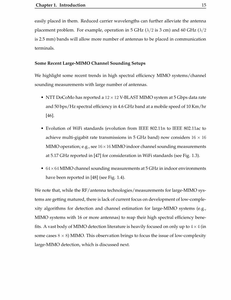
• Evolution of WiFi standards (evolution from IEEE 802.11n to IEEE 802.11ac to
achieve multi-gigabit rate transmissions in 5 GHz band) now considers 16 × 16
MIMO operation; e.g., see 16×16 MIMO indoor channel sounding measurements
at 5.17 GHz reported in [47] for consideration in WiFi standards (see Fig. 1.3).
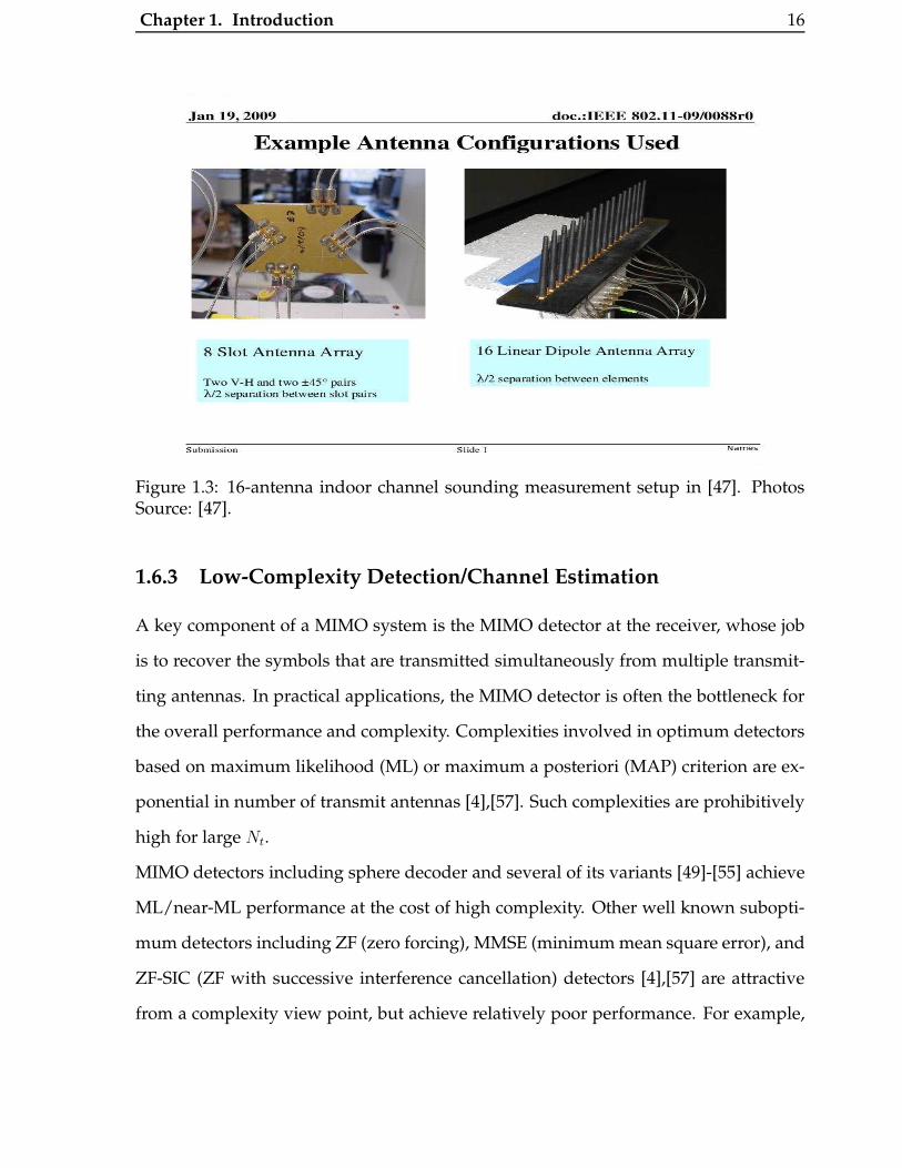
• 64×64 MIMO channel sounding measurements at 5 GHz in indoor environments
have been reported in [48] (see Fig. 1.4).
We note that, while the RF/antenna technologies/measurements for large-MIMO sys-
tems are getting matured, there is lack of current focus on development of low-comple-
xity algorithms for detection and channel estimation for large-MIMO systems (e.g.,
MIMO systems with 16 or more antennas) to reap their high spectral efficiency bene-
fits. A vast body of MIMO detection literature is heavily focused on only up to 4×4 (in
some cases 8× 8) MIMO. This observation brings to focus the issue of low-complexity
large-MIMO detection, which is discussed next.
Chapter 1. Introduction 16
Figure 1.3: 16-antenna indoor channel sounding measurement setup in [47]. PhotosSource: [47].
1.6.3 Low-Complexity Detection/Channel Estimation
A key component of a MIMO system is the MIMO detector at the receiver, whose job
is to recover the symbols that are transmitted simultaneously from multiple transmit-
ting antennas. In practical applications, the MIMO detector is often the bottleneck for
the overall performance and complexity. Complexities involved in optimum detectors
based on maximum likelihood (ML) or maximum a posteriori (MAP) criterion are ex-
ponential in number of transmit antennas [4],[57]. Such complexities are prohibitively
high for large Nt.
MIMO detectors including sphere decoder and several of its variants [49]-[55] achieve
ML/near-ML performance at the cost of high complexity. Other well known subopti-
mum detectors including ZF (zero forcing), MMSE (minimum mean square error), and
ZF-SIC (ZF with successive interference cancellation) detectors [4],[57] are attractive
from a complexity view point, but achieve relatively poor performance. For example,

Chapter 1. Introduction 17
(a) 64-Antenna/RF hardware at 5 GHz (b) LOS setup
Figure 1.4: 64 × 64 MIMO indoor channel sounding setup at 5 GHz reported in [48].Photos Source: [48].
the ZF-SIC detector(i.e., the well known V-BLAST detector with ordering [18],[58]
)
does not achieve the full diversity in the system; diversity achieved by ZF-SIC detector
in V-BLAST is only Nr−Nt +1 [1]. Also, the per-symbol complexity of ZF-SIC detector
is cubic in number of transmit antennas, which is still high for large Nt. Therefore,
there is a need for large-MIMO detectors which can perform close to the performance
of the optimum detector, but at practically affordable complexities.
Recent Developments in Large-MIMO Detection
In this context, we note that certain algorithms rooted in neural networks/machine
learning/artificial intelligence have been shown to achieve near-optimal performance
in multiuser detection of CDMA signals, when the number of users in the system gets
large. Some of these algorithms include local neighborhood likelihood ascent search
(LAS) algorithm [59], probabilistic data association (PDA) [60]-[62], and belief prop-
agation (BP) [67]-[69]. Motivated by the suitability of such algorithms for multiuser detec-
tion in large CDMA systems, in this thesis, we successfully develop two of these algorithms,
namely, LAS and PDA algorithms, in the context of large-MIMO detection, and establish that
Chapter 1. Introduction 18
near-optimal detection can be achieved in large-MIMO systems at practically affordable com-
plexities. For e.g., the per-symbol complexity of the LAS algorithm is only quadratic in
number of transmit antennas for Nt = Nr V-BLAST MIMO, which makes the algorithm
amenable for practical implementations. Specifically, following our reporting of the
LAS algorithm for large-MIMO detection in [70],[71], an FPGA/ASIC implementation
of the LAS algorithm for 32 × 32 V-BLAST MIMO with 4-/16-/64-QAM has been re-
ported in [72]. We expect that investigation and reporting of more of such large-MIMO
detection algorithms and implementations will follow in the coming years. For e.g.,
a reactive tabu search (RTS) based algorithm and two BP based algorithms for large-
MIMO detection (in 32×32 and 64×64 MIMO) have been reported recently in [73],[74]
and [75],[76]. Another large-MIMO detection algorithm (e.g., in 50× 50 MIMO) based
on Gibbs sampling has been reported recently in [77].
We further note that CSIR is needed for MIMO detection. So, accurate channel estima-
tion at the receiver is crucial. For large-MIMO systems, the NtNr number of channel
coefficients to be estimated is large. We propose a pilot-assisted training based iterative
detection/channel estimation scheme for this purpose [78].
With the feasibility of such low-complexity algorithms, detection/channel estimation need not
be a bottleneck to implement large-MIMO systems. This message is one of the key contributions
made in this thesis.
1.7 Problems Addressed and Contributions Made
The work reported in this thesis is comprised of the following three major parts:
1. Low-complexity detection, based on a local neighborhood search and probabilis-
tic data association, on large-MIMO links with CSIR only, and the associated
channel estimation. (Chapters 2, 3, 4).
Chapter 1. Introduction 19
2. Low-complexity precoding using X-Codes/X-Precoders and Y-Codes/Y-Preco-
ders on large-MIMO links with CSIT and CSIR. (Chapters 5, 6).
3. Low-complexity precoding for large multiuser MISO downlink systems with CSIT,
based on vector perturbation with a reduced search space. (Chapter 7).
1.7.1 Low-Complexity Large-MIMO Detection/Channel Estimation
In this part of the thesis, we present two low-complexity large-MIMO detection al-
gorithms and their uncoded/coded bit error performances in i.i.d. and spatially cor-
related MIMO channels. The first algorithm is a multistage LAS (M-LAS) algorithm
based on a local neighborhood search with ML cost as the search metric [70],[71],[79]-
[82]. The second algorithm is the PDA algorithm based on MAP criterion [83]. The
performance of these two algorithms are evaluated for the two popular MIMO ar-
chitectures, namely, i) V-BLAST MIMO, and ii) non-orthogonal STBC MIMO. While
V-BLAST MIMO exploits only spatial dimensions to achieve full rate(i.e., maximum
multiplexing gain of min(Nt, nr)), fully diverse non-orthogonal STBC MIMO [21] ex-
ploits spatial and time dimensions to achieve both full diversity (NtNr) as well as full
rate.
Multistage Likelihood Ascent Search
The LAS algorithm starts with an initial solution vector, which can be, for e.g., MF so-
lution vector or ZF solution vector or MMSE solution vector. A neighborhood around
the initial vector is defined; e.g., set of all vectors which differ from the initial solution
vector in one coordinate is an example of a neighborhood. For each of the vectors in the
neighborhood, the algorithm computes the ML cost function. The best vector among
the neighboring vectors (in terms of least ML cost among them) which also happens to
have a lesser ML cost than that of the initial vector is chosen, and declared as the new
solution vector. This new solution vector is passed on as the initial vector for the next
Chapter 1. Introduction 20
iteration, where the best vector among the neighboring vectors of the current initial
vector is chosen as the new solution vector for the next iteration, and so on until a local
minima is reached. The algorithm ends once a local minima is encountered, and the
local minima is declared as the final solution vector.
LAS Algorithm Complexity:
A key advantage of the LAS algorithm is its simplicity in its search operation. Much
of the algorithm complexity arises from the initial vector computation (which involves
matrix inversion operation in ZF and MMSE solutions) and the computation of HTH,
which requires O(NtNr) complexity per symbol. The average per-symbol complexity
in the search part alone is found to be O(Nt) through simulations. So the overall per-
symbol complexity of the LAS algorithm is O(NtNr). This low order of complexity is
well suited for scaling to large number of dimensions.
LAS Algorithm Performance:
A even more interesting aspect of the LAS algorithm is that its bit error rate (BER) per-
formance improves with increasing values of Nt = Nr in V-BLAST MIMO; a behavior
we refer to as the ’large-system behavior’ of the algorithm. Increasingly closer to ML
performance is achieved for increasing number of transmit antennas.
Applicability to Large Non-Orthogonal STBC MIMO Systems:
We note that large number of dimensions are required for achieving near-optimal per-
formance with LAS. Since STBCs code across both space and time, it is possible to
achieve large number of dimensions in STBC MIMO systems with lesser number of
antennas as compared to V-BLAST MIMO systems. For example, hundreds of di-
mensions can be created with tens of dimensions each in space and time using non-
orthogonal STBCs which achieve both full rate (same as that achieved in V-BLAST) as
well as full transmit diversity [21]. For example, a 16×16 non-orthogonal STBC matrix
in [21] is constructed using 256 complex data symbols resulting in 512 real dimensions;
with 64-QAM and rate-3/4 turbo code, this STBC achieves a spectral efficiency of 72

Chapter 1. Introduction 21
bps/Hz. In Chapter 2, we establish through extensive simulations that the LAS algo-
rithm is very effective, both in terms of complexity as well as achieving near-ML/near
capacity performance, in decoding 16× 16 and 32× 32 non-orthogonal STBCs, even in
the presence of spatial correlation and with estimated channel matrix.
Multistage LAS:
In an attempt to improve the performance of the basic LAS algorithm, we propose
a more general version of LAS algorithm, termed as multistage LAS algorithm. This
algorithm executes an escape mechanism when it encounters a local minima, by chang-
ing the neighborhood definition: it considers vectors which differ in two or more co-
ordinates (as opposed to only one coordinate in the basic neighborhood definition in
LAS) as neighbors. On escaping from a local minima, the algorithm reverts back to
the basic neighborhood definition till the next local minima is encountered and stops
when no escape from a local minima is possible.
Our contributions in this part can be summarized as follows [70],[71],[78]-[82]:
• We develop the basic LAS algorithm with 1-symbol neighborhood for use in V-
BLAST and non-orthogonal STBC MIMO systems. We show that LAS detection
of 64×64 and 128×128 V-BLAST MIMO signals (i.e., Nt = Nr = 64, 128) achieves
close to SISO AWGN performance1. In a 128×128 V-BLAST system with 4-QAM,
LAS algorithm achieves an uncoded BER of 10−3 at an SNR of just about 1 dB
away from SISO AWGN performance. In terms of coded BER, with a rate-3/4
turbo code at a spectral efficiency of 192 bps/Hz, the algorithm performs close to
within about 4.5 dB from theoretical MIMO capacity.
• We generalize the basic 1-symbol neighborhood LAS algorithm by employing a
low-complexity multistage multi-symbol neighborhood based strategy; we refer
1Since simulation of brute-force ML or sphere decoder is prohibitively complex for such large di-mensions, we use the SISO AWGN performance as a lower bound on the true ML performance forcomparison purposes.
Chapter 1. Introduction 22
to this as multistage LAS (M-LAS) algorithm. We show that the M-LAS algo-
rithm outperforms the basic LAS algorithm with some increase in complexity.
• We propose a method to generate soft outputs from the M-LAS output vector.
The proposed soft outputs generation for the individual bits results in about 1 to
1.5 dB improvement in coded BER compared to hard decision M-LAS outputs.
• Assuming i.i.d. fading and perfect CSIR, our simulation results show that the
proposed M-LAS algorithm is able to decode large non-orthogonal STBCs (e.g.,
16 × 16 and 32 × 32 STBCs) and achieve near SISO AWGN uncoded BER per-
formance as well as near-capacity (within 4 dB from theoretical MIMO capacity)
coded BER performance.
• Using the proposed detector, we decode and report the simulated BER perfor-
mance of ‘perfect codes’ [22],[84]-[87] of large dimensions.
• Presenting a BER performance and complexity comparison of the proposed non-
orthogonal STBC/LAS detection approach with other large-MIMO/detector ap-
proaches (e.g., stacked Alamouti codes/QOSTBCs and associated interference
canceling receivers reported in [88]), we show that the proposed approach out-
performs the other considered approaches, both in terms of performance as well
as complexity.
• We present simulation results that quantify the loss in BER performance due to
spatial correlation in large-MIMO systems, by considering a more realistic spa-
tially correlated MIMO fading channel model proposed by Gesbert et al in [8]. We
show that this loss in performance can be alleviated by providing more receive
dimensions (i.e., more receive antennas than transmit antennas).
• We present a training-based iterative detection/channel estimation scheme for
Chapter 1. Introduction 23
large non-orthogonal STBC MIMO systems. We report BER and nearness-to-
capacity results when the channel matrix is estimated using the proposed iter-
ative scheme and compare these results with those obtained using perfect CSIR
assumption.
• We present an asymptotic (Nt, Nr → ∞, keeping Nt = Nr) performance analysis
of the basic LAS algorithm detection in V-BLAST MIMO with 4-QAM in i.i.d.
Rayleigh fading with a motivation to get some insights that can explain the good
performance of the LAS algorithm in large dimensions.
Probabilistic Data Association
PDA algorithm was originally developed for target tracking. It is widely used in digital
communications [60]-[66]. Particularly, PDA algorithm is a reduced complexity alter-
native to the a posteriori probability (APP) decoder/detector/equalizer. Near-optimal
performance has been demonstrated for PDA-based multiuser detection in CDMA sys-
tems with large number of users [60]-[62]. PDA has been used in the detection of V-
BLAST signals with small number of antennas [64]-[66]. Here, we develop the PDA
algorithm for use in large V-BLAST as well as non-orthogonal STBC MIMO detection,
and present its uncoded and coded BER performance [83]. The complexity of PDA is
more than that of LAS. PDA is shown to perform better than LAS in higher-order QAM
(e.g., 16-QAM) at low SNRs.
1.7.2 Low-Complexity Large-MIMO Precoding Using X-, Y-Codes
In this part of the thesis, we consider MIMO systems where CSI is fully available both
at the transmitter and the receiver. It is known that precoding techniques can provide
large performance improvements in such scenarios. A popular precoding approach
is based on singular value decomposition (SVD) [89],[90] of the channel so that the
MIMO channel can be seen as parallel channels.
Chapter 1. Introduction 24
In slow fading scenarios, channels are subject to block fading. Without rate and power
adaptation, outages cannot be avoided. In such scenarios, a popular measure of relia-
bility is the diversity order achieved by a given transmit-receive scheme. We consider
SVD precoding for MIMO systems, which transforms the MIMO channels into paral-
lel subchannels. At the receiver, ML decoding (MLD) can be employed separately for
each subchannel. To improve the low diversity order of the SVD precoded system,
we propose some simple linear codes prior to SVD precoding. These codes are named
X- and Y-Codes due to the structure of the encoder matrix, which enables us to flexi-
bly pair subchannels with different diversity orders. Specifically, the subchannels with
low diversity orders can be paired together with those having high diversity orders,
so that the overall diversity order is improved. The main contributions in this part are
[93],[94]:
1. X-Codes: A set of 2-dimensional (2-D) real orthogonal matrices is used to jointly
code over pairs of subchannels, without increasing the transmit power. Since the
matrices are effectively parameterized with a single angle, the design of X-Codes
primarily involves choosing the optimal angle for each pair of subchannels. The
angles are chosen a priori and do not change with each channel realization. This
is why we use the term ‘Code’ instead of ‘Precoder’. Further optimization of an-
gles are based upon minimizing the average error performance. At the receiver,
we show that the MLD can be easily accomplished using Nr low complexity 2-D
real sphere decoders (SD) [49]. It is shown that X-Codes have better error per-
formance than that of other precoders, yet it becomes worse when the pair of
subchannels is poorly conditioned. This motivates us to propose Y-Codes.
2. Y-Codes: Instead of using rotation for pairing subchannels, we use a linear code
generator matrix which is upper left triangular. Y-Codes are parameterized with
2 parameters corresponding to power allocated to the two subchannels. These
parameters are computed so as to minimize the average error probability. The

Chapter 1. Introduction 25
MLD complexity is the same as that of the scalar channels in linear precoders
[25],[26] and is less than that of the X-Codes, while the performance of Y-Codes
is better than that of X-Codes for ill-conditioned channel pairs
3. X-, Y-Precoders: The X- and Y-Precoders employ the same pairing structure as that
in X-, Y-Codes. However, the code generator matrix for each pair of subchannels
is chosen for each channel realization. We observed that the error performance of
X- and Y-Precoders is better than that of X- and Y-Codes.
Precoding Using X-Codes to Increase MIMO Capacity with Discrete Alphabets
It is known that the capacity of the Gaussian MIMO channel with CSIT can be achieved
with Gaussian inputs. However, in practice, the input alphabet is not Gaussian and is
generally chosen from a finite signal set. Therefore, precoders should be designed
to achieve the capacity of the Gaussian MIMO channel with discrete input alphabets.
The optimal precoder with discrete inputs is given by a fixed point equation, which re-
quires a high complexity numerical evaluation [95]. Since the optimal precoder jointly
codes all the Nt inputs, joint decoding is also required at the receiver. Thus, the decod-
ing complexity can be very high, specially for large Nt. Motivated by this issue of high
complexity of the optimal precoder with discrete inputs, we propose a precoder based
on X-Codes, which is shown to achieve mutual information close to the discrete input
MIMO capacity, at low complexity [96],[97].
The structure of X-Codes enables us to express the total mutual information as a sum
of the mutual information of all the pairs of subchannels. The problem of finding the
optimal precoder with the above structure, which maximizes the total mutual infor-
mation, is solved by i) optimizing the rotation angle and the power allocation within
each pair, and ii) finding the optimal pairing and power allocation among the pairs.
It is shown that the mutual information achieved with the proposed pairing scheme
is very close to that achieved with the optimal precoder by Cruz et al. [95], and is
Chapter 1. Introduction 26
significantly better than Mercury/waterfilling strategy by Lozano et al. [98]. Our ap-
proach greatly simplifies both the precoder optimization and the detection complexity,
making it suitable for practical applications.
1.7.3 Low-Complexity Large Multiuser MISO Precoding
In this part of the work, we consider the problem of precoding in large multiuser MISO
systems with large number of transmit antennas (Nt) at the base station and large num-
ber of downlink users (Nu), where each user has one receive antenna. Such large MISO
systems are of interest because of the high capacities (sum-rates) of the order of tens to
hundreds of bits/channel use possible in such systems. We propose a vector perturba-
tion based low-complexity precoder, termed as norm descent search (NDS) precoder
[99], which has a complexity of just O(NuNt) per information symbol. This low com-
plexity attribute of the precoder is achieved by searching for the perturbation vector
over a reduced search space. Interestingly, in terms of BER performance, the proposed
precoder achieves increasingly better BER for increasing Nt, Nu, making it suited for
large MISO systems both in terms of complexity as well as performance.
1.8 Organization of the Thesis
The rest of the thesis is organized as follows. In Chapter 2, we present the proposed M-
LAS algorithm and its uncoded and turbo coded BER performance in large V-BLAST
MIMO and non-orthogonal STBC MIMO systems. Performance of the M-LAS algo-
rithm with estimated CSIR using an iterative detection/channel estimation scheme is
also presented in this chapter. In Chapter 3, we present the asymptotic performance
analysis of the LAS algorithm. In Chapter 4, we present the PDA algorithm, its BER
performance and complexity in large-MIMO detection. In Chapter 5, we present the

Chapter 1. Introduction 27
proposed large-MIMO precoding schemes using X-Codes/Precoders and Y-Codes/Pr-
ecoders and their performance. In Chapter 6, the precoder based on X-Codes to in-
crease the mutual information in Gaussian MIMO channels with discrete input alpha-
bets is presented. In Chapter 7, the proposed vector perturbation based large multiuser
MISO precoding scheme that uses a low-complexity norm descent search is presented.
Finally, conclusions are presented in Chapter 8.

Chapter 2
Large-MIMO Detection Using
Likelihood Ascent Search
In this Chapter, we present a low-complexity detection algorithm, termed as likeli-
hood ascent search (LAS) algorithm, suited for large-MIMO detection, and evaluate its
uncoded and coded BER performance [70],[71],[78]-[82]. The LAS algorithm is a lo-
cal neighborhood search algorithm. The neighborhood of a initial solution vector in a
given iteration of the algorithm is defined as a collection of those vectors which differ
in certain number of coordinates compared to the initial solution vector. Better solu-
tion vectors compared to the initial solution vector (in terms of maximum-likelihood
cost) in this neighborhood are searched for. The best among the neighbors is fed as
the initial solution vector for the next iteration. The iterations are continued till a local
minima is reached, upon which the local minima is declared as the solution vector, or
an escape strategy is adopted to leave the local minima and continue the search for bet-
ter local minimas. The LAS algorithm is shown to exhibit large-system effect, where
the BER performance improves with increasing number of antennas. We also show
that the algorithm achieves near-capacity performance within about 4 dB from the the-
oretical limit. We investigate the effect of spatial correlation on the BER performance
of the LAS algorithm. An iterative detection/channel estimation scheme and its BER
28
Chapter 2. Large-MIMO Detection Using Likelihood Ascent Search 29
performance are also presented.
This chapter is organized as follows. In Section 2.1, we present the system models
for V-BLAST MIMO and non-orthogonal STBC MIMO. In Section 2.2, the proposed
multistage LAS algorithm is presented. The BER performance of LAS detection in
large V-BLAST MIMO and non-orthogonal STBC MIMO are presented in Sections 2.3
and 2.4, respectively. The proposed iterative detection/channel estimation scheme and
its performance are presented in Section 2.5.
2.1 System Model
In this section, we present system models corresponding to V-BLAST MIMO and non-
orthogonal STBC MIMO, and a unified system model covering both models so that the
LAS detection algorithm can be presented under the unified framework.
2.1.1 V-BLAST MIMO
Consider a V-BLAST system with Nt transmit antennas and Nr receive antennas, Nt ≤
Nr, where Nt symbols are transmitted from Nt transmit antennas simultaneously. Let
xc ∈ CNt be the symbol vector transmitted. Each element of xc is an M-PAM or M-
QAM symbol. Let Hc ∈ CNr×Nt be the channel gain matrix, such that the (p, q)th entry
hp,q is the complex channel gain from the qth transmit antenna to the pth receive an-
tenna. Assuming rich scattering, we model the entries of Hc as i.i.d CN (0, 1). Let
yc ∈ CNr and nc ∈ CNr denote the received signal vector and the noise vector, re-
spectively, at the receiver, where the entries of nc are modeled as i.i.d CN (0, σ2). The
received signal vector can then be written as
yc = Hcxc + nc. (2.1)
Chapter 2. Large-MIMO Detection Using Likelihood Ascent Search 30
Let yc, Hc, xc, and nc be decomposed into real and imaginary parts as follows:
yc = yI + jyQ, xc = xI + jxQ, nc = nI + jnQ, Hc = HI + jHQ. (2.2)
Further, we define Hr ∈ R2Nr×2Nt , yr ∈ R2Nr , xr ∈ R2Nt , and nr ∈ R2Nr as
Hr =
HI −HQ
HQ HI
, yr = [yT
I yTQ]T , xr = [xT
I xTQ]T , nr = [nT
I nTQ]T .
Now, (2.1) can be written as
yr = Hrxr + nr. (2.3)
We will work with the real-valued system in (2.3). For notational simplicity, we drop
subscripts r in (2.3) and write
y = Hx + n, (2.4)
where H = Hr ∈ R2Nr×2Nt , y = yr ∈ R2Nr , x = xr ∈ R2Nt and n = nr ∈ R2Nr .
With the above real-valued system model, the real-part of the original complex data
symbols will be mapped to [x1, · · · , xNt ] and the imaginary-part of these symbols will
be mapped to [xNt+1, · · · , x2Nt ].
2.1.2 Non-Orthogonal STBC MIMO
Consider a STBC MIMO system with multiple transmit and multiple receive antennas.
An (n, p, k) STBC is represented by a matrix Xc ∈ Cn×p, where n and p denote the
number of transmit antennas and number of time slots, respectively, and k denotes the
number of complex data symbols sent in one STBC matrix [2]. The (i, j)th entry in Xc
represents the complex number transmitted from the ith transmit antenna in the jth
time slot. The rate of an STBC, r, is given by r4= k
p. Let Nr and Nt = n denote the

Chapter 2. Large-MIMO Detection Using Likelihood Ascent Search 31
number of receive and transmit antennas, respectively. Let Hc ∈ CNr×Nt denote the
channel gain matrix, where the (i, j)th entry in Hc is the complex channel gain from
the jth transmit antenna to the ith receive antenna. We assume that the channel gains
remain constant over one STBC matrix duration. Assuming rich scattering, we model
the entries of Hc as i.i.d CN (0, 1). The received space-time signal matrix, Yc ∈ CNr×p,
can be written as
Yc = HcXc + Nc, (2.5)
where Nc ∈ CNr×p is the noise matrix at the receiver and its entries are modeled as i.i.d
CN(0, σ2
). The (i, j)th entry in Yc is the received signal at the ith receive antenna in
the jth time slot. In a linear dispersion (LD) STBC, Xc can be decomposed into a linear
combination of weight matrices corresponding to each data symbol and its conjugate
as [2]
Xc =
k∑
i=1
x(i)c A(i)
c + (x(i)c )∗E(i)
c , (2.6)
where x(i)c is the ith complex data symbol, and A
(i)c ,E
(i)c ∈ CNt×p are its corresponding
weight matrices. The detection algorithm we present in this Chapter can decode gen-
eral LD STBCs of the form in (2.6). For the purpose of simplicity in exposition, here we
consider a subclass of LD STBCs, where Xc can be written in the form
Xc =
k∑
i=1
x(i)c A(i)
c . (2.7)
From (2.5) and (2.7), applying the vec (.) operation we have
vec (Yc) =k∑
i=1
x(i)c vec (HcA
(i)c ) + vec (Nc). (2.8)
Chapter 2. Large-MIMO Detection Using Likelihood Ascent Search 32
If U,V,W,D are matrices such that D = UWV, then it is true that vec (D) = (VT ⊗
U) vec (W), where ⊗ denotes tensor product of matrices [108]. Using this, we can write
(2.8) as
vec (Yc) =
k∑
i=1
x(i)c (Ip ⊗Hc) vec (A(i)
c ) + vec (Nc). (2.9)
Further, define yc4= vec (Yc), Hc
4= (I ⊗Hc), a
(i)c
4= vec (A
(i)c ), and nc
4= vec (Nc). From
these definitions, it is clear that yc ∈ CNrp, Hc ∈ CNrp×Ntp, a(i)c ∈ CNtp, and nc ∈ CNrp.
Let us also define a matrix Hc ∈ CNrp×k, whose ith column is Hc a(i)c , i = 1, · · · , k. Let
xc ∈ Ck, whose ith entry is the data symbol x(i)c . With these definitions, we can write
(2.9) as
yc =k∑
i=1
x(i)c (Hc a
(i)c ) + nc = Hcxc + nc. (2.10)
Let yc, Hc, xc, and nc be decomposed into real and imaginary parts as
yc = yI + jyQ, xc = xI + jxQ, nc = nI + jnQ, Hc = HI + jHQ. (2.11)
Further, we define xr ∈ R2k, yr ∈ R2Nrp, Hr ∈ R2Nrp×2k, and nr ∈ R2Nrp as
Hr =
HI − HQ
HQ HI
, nr = [nT
I nTQ]T , xr = [xT
I xTQ]T , yr = [yT
I yTQ]T . (2.12)
Now, (2.10) can be written as
yr = Hrxr + nr. (2.13)

Chapter 2. Large-MIMO Detection Using Likelihood Ascent Search 33
We will work with the real-valued system in (2.13). For notational simplicity, we drop
subscripts r in (2.13) and write
y = Hx + n, (2.14)
where H = Hr ∈ R2Nrp×2k, y = yr ∈ R2Nrp, x = xr ∈ R2k, and n = nr ∈ R2Nrp.
2.1.3 High-rate Non-orthogonal STBCs from CDA
We focus on the detection of square (i.e., n = p = Nt), full-rate (i.e., k = pn = N2t ), cir-
culant (where the weight matrices A(i)c ’s are permutation type), non-orthogonal STBCs
from CDA, whose construction for arbitrary number of transmit antennas n is given
by the matrix in (2.15) given by [21]:
Xc =
∑n−1i=0 x0,i ti δ
∑n−1i=0 xn−1,i ωi
n ti δ∑n−1
i=0 xn−2,i ω2in ti · · · δ
∑n−1i=0 x1,i ω
(n−1)in ti
∑n−1i=0 x1,i ti
∑n−1i=0 x0,i ωi
n ti δ∑n−1
i=0 xn−1,i ω2in ti · · · δ
∑n−1i=0 x2,i ω
(n−1)in ti
∑n−1i=0 x2,i ti
∑n−1i=0 x1,i ωi
n ti∑n−1
i=0 x0,i ω2in ti · · · δ
∑n−1i=0 x3,i ω
(n−1)in ti
......
......
...∑n−1
i=0 xn−2,i ti∑n−1
i=0 xn−3,i ωin ti
∑n−1i=0 xn−4,i ω2i
n ti · · · δ∑n−1
i=0 xn−1,i ω(n−1)in ti
∑n−1i=0 xn−1,i ti
∑n−1i=0 xn−2,i ωi
n ti∑n−1
i=0 xn−3,i ω2in ti · · · ∑n−1
i=0 x0,i ω(n−1)in ti
.
(2.15)
In (2.15), ωn = ej2πn , and xu,v, 0 ≤ u, v ≤ n − 1 are the data symbols from a QAM al-
phabet. When δ = e√
5 j and t = ej, the STBC in (2.15) achieves full transmit diversity
(under ML decoding) as well as information-losslessness [21]. When δ = t = 1, the
code ceases to be of full-diversity (FD), but continues to be information-lossless (ILL)
[109],[110]. High spectral efficiencies with large n can be achieved using this code con-
struction. For example, with n = 32 transmit antennas, the 32 × 32 STBC from (2.15)
with 16-QAM and rate-3/4 turbo code achieves a spectral efficiency of 96 bps/Hz. This

Chapter 2. Large-MIMO Detection Using Likelihood Ascent Search 34
high spectral efficiency is achieved along with the full-diversity of order nNr. How-
ever, since these STBCs are non-orthogonal, ML detection gets increasingly impractical
for large n. Consequently, a key challenge in realizing the benefits of these large STBCs
in practice is that of achieving near-ML performance for large n at low detection com-
plexities. The multistage likelihood ascent search (M-LAS) detector proposed in Sec. 2.2
essentially addresses this challenging issue.
2.1.4 Unified System Model
A unified linear vector channel model for both V-BLAST MIMO and non-orthogonal
STBC MIMO is given by
y = Hx + n, (2.16)
where H ∈ R2Nrp×2k is the equivalent matrix of channel gains, y ∈ R
2Nrp is the equiv-
alent received signal vector, x ∈ R2k is the equivalent transmitted symbol vector, and
n ∈ R2Nrp is the equivalent additive white Gaussian noise vector. We can get the V-
BLAST MIMO system model by simply substituting p = 1 and k = Nt in (2.16). Simi-
larly, we can get the non-orthogonal STBC MIMO system model by substituting p = Nt
and k = N2t .
The transmitted symbols are assumed to be M-QAM. For simplicity, we consider
square-QAM. However, the algorithm is valid for rectangular QAM as well. The ith
element of x, xi is therefore a√M-PAM symbol and takes discrete values from the set
Ai = {Am, m = 1, · · · ,√M}, where Am = (2m − 1 −
√M). In both V-BLAST MIMO
and non-orthogonal STBC MIMO, the average signal power received at each receive
antenna is NtEs, where Es is the average energy of each transmitted symbol. There-
fore, the average SNR at each receive antenna is given by γ = NtEs
σ2 [2]. Now, define a
2k-dimensional signal space S to be the Cartesian product of A1 to A2k.
Chapter 2. Large-MIMO Detection Using Likelihood Ascent Search 35
2.1.5 Maximum-Likelihood Detector
The maximum-likelihood (ML) detector is the optimal detector w.r.t minimizing the
word error probability. One word corresponds to one Nt dimensional transmitted sym-
bol vector in case of V-BLAST. In the case of non-orthogonal STBC MIMO, one word
corresponds to one Nt ×Nt STBC codeword matrix. The ML decision rule is given by
dML =arg min
d ∈ S‖y −Hd‖2
=arg min
d ∈ SdTHTHd− 2yTHd, (2.17)
whose complexity is exponential in k [57]. So, detection algorithms which are low
in complexity but close to ML in terms of performance are of interest in large-MIMO
systems, where k is large.
ML Performance in Large Dimensions: Since we are interested in detectors with perfor-
mance close to the ML performance, it would be necessary to know the true ML per-
formance for comparison purposes. However, exact analytical expressions do not exist
for the word or bit error probability of V-BLAST and non-orthogonal STBC MIMO
with ML detection. It is also difficult to know the error probabilities from Monte-Carlo
simulation of ML detection (except for systems with small dimensions) due to the ex-
ponential complexity in number of dimensions. Even sphere decoder, which is known
to achieve ML performance, and its low-complexity variants do not scale well for large
dimensions. Further, ML detector is optimal w.r.t. the word error probability. In many
applications, bit and symbol error rates are more relevant performance measures. The
detector which achieves minimum BER is called as the minimum BER detector [57].
Just like for ML detection, exact analytical expressions do not exist for the minimum
BER detector. Because of this (i.e., due to lack of low-complexity methodologies to
evaluate the exact ML or minimum BER detectors’ performance for large dimensions),

Chapter 2. Large-MIMO Detection Using Likelihood Ascent Search 36
instead of comparing with the exact BER performance of ML/minimum BER detec-
tors, we will compare the BER performance of the proposed detectors with the BER
performance on single-input single-output (SISO) unfaded AWGN channel, which is a
lower bound on the BER performance in MIMO fading channels.
2.2 Proposed Multistage LAS Detector
In this section, we present the proposed multistage LAS (M-LAS) algorithm for large-
MIMO detection.
The M-LAS algorithm consists of a sequence of likelihood-ascent search stages, where
the likelihood increases monotonically with every search stage. Each search stage con-
sists of several sub-stages. There can be at most M sub-stages, each consisting of one
or more iterations (the first sub-stage can have one or more iterations, whereas all the
other sub-stages can have at most one iteration). In the first sub-stage, the algorithm
updates one symbol per iteration such that the likelihood monotonically increases from
one iteration to the next until a local minima is reached. Upon reaching this local min-
ima, the algorithm initiates the second sub-stage. In the second sub-stage, a 2-symbol
update is tried to further increase the likelihood. If the algorithm succeeds in increasing
the likelihood by 2-symbol update, it starts the next search stage. If the algorithm does
not succeed in the second sub-stage, it goes to the third sub-stage where a 3-symbol
update is tried to further increase the likelihood. Essentially, in the Kth sub-stage, a
K-symbol update is tried to further increase the likelihood. This goes on until a) either
the algorithm succeeds in the Kth sub-stage for some K ≤ M (in which case a new
search stage is initiated), or b) the algorithm terminates.
The M-LAS algorithm starts with an initial solution d(0), given by d(0) = By, where
B is the initial solution filter, which can be a matched filter (MF) or zero-forcing (ZF)
filter or MMSE filter. The index m in d(m) denotes the iteration number in a sub-stage
of a given search stage. The ML cost function after the kth iteration in a given search

Chapter 2. Large-MIMO Detection Using Likelihood Ascent Search 37
stage is
C(k) = d(k)T
HTHd(k) − 2yTHd(k). (2.18)
2.2.1 One-symbol Update
In the (k + 1)th iteration, a one-symbol update tries to increase the likelihood by up-
dating exactly one entry of the current data vector d(k). Let us assume that we update
the pth symbol in the (k + 1)th iteration; in V-BLAST p can take value from 1, · · · , Nt
forM-PAM and 1, · · · , 2Nt forM-QAM. The update rule can be written as
d(k+1) = d(k) + λ(k)p ep, (2.19)
where ep denotes the unit vector with its pth entry only as one, and all other entries
as zero. Also, for any iteration k, d(k) should belong to the space S, and therefore
λ(k)p can take only certain integer values. For example, in case of 4-PAM or 16-QAM(both have the same signal set Ap = {−3,−1, 1, 3}
), λ
(k)p can take values only from
{−6,−4,−2, 0, 2, 4, 6}. Using (2.18) and (2.19), and defining a matrix G as
G4= HTH, (2.20)
we can write the cost difference as
∆Ck+1p
4= C(k+1) − C(k)
= λ(k)2
p (G)p,p − 2λ(k)p z(k)
p , (2.21)
where hp is the pth column of H, z(k) = HT (y −Hd(k)), z(k)p is the pth entry of the z(k)
vector, and (G)p,p is the (p, p)th entry of the G matrix. Also, let us define ap and l(k)p as
ap = (G)p,p , l(k)p = |λ(k)
p |. (2.22)
Chapter 2. Large-MIMO Detection Using Likelihood Ascent Search 38
With the above variables defined, we can rewrite (2.21) as
∆Ck+1p = l(k)2
p ap − 2l(k)p |z(k)
p | sgn(λ(k)p ) sgn(z(k)
p ), (2.23)
where sgn(.) denotes the signum function. For the ML cost function to reduce from the
kth to the (k +1)th iteration, the cost difference should be negative. Using this fact and
that ap and l(k)p are non-negative quantities, we can conclude from (2.23) that the sign
of λ(k)p must satisfy
sgn(λ(k)p ) = sgn(z(k)
p ). (2.24)
Using (2.24) in (2.23), the ML cost difference can be rewritten as
F(l(k)p )
4= ∆Ck+1
p = l(k)2
p ap − 2l(k)p |z(k)
p |. (2.25)
For F(l(k)p ) to be non-positive, the necessary and sufficient condition from (2.25) is that
l(k)p <
2|z(k)p |
ap. (2.26)
However, we can find the value of l(k)p which satisfies (2.26) and at the same time gives
the largest descent in the ML cost function from the kth to the (k +1)th iteration (when
symbol p is updated). Also, l(k)p is constrained to take only certain integer values, and
therefore the brute-force way to get optimum l(k)p is to evaluate F(l
(k)p ) at all possible
values of l(k)p . This would become computationally expensive as the constellation size
M increases. However, for the case of 1-symbol update, we could obtain a closed-form
expression for the optimum l(k)p that minimizes F(l
(k)p ), which is given by (correspond-
ing theorem and proof are given in the Appendix A)
l(k)p,opt = 2
⌊|z(k)
p |2ap
⌉, (2.27)
Chapter 2. Large-MIMO Detection Using Likelihood Ascent Search 39
where b.e denotes the rounding operation, where for a real number x, bxe is the integer
closest to x. If the pth symbol in d(k), i.e., d(k)p , were indeed updated, then the new value
of the symbol would be given by
d(k+1)p = d(k)
p + l(k)p sgn(z(k)
p ). (2.28)
However, d(k+1)p can take values only in the set Ap, and therefore we need to check for
the possibility of d(k+1)p being greater than (M− 1) or less than −(M− 1). If d
(k+1)p >
(M− 1), then l(k)p is adjusted so that the new value of d
(k+1)p with the adjusted value of
l(k)p using (2.28) is (M−1). Similarly, if d
(k+1)p < −(M−1), then l
(k)p is adjusted so that the
new value of d(k+1)p is−(M−1). Let l
(k)p,opt be obtained from l
(k)p,opt after these adjustments.
It can be shown that if F(l(k)p,opt) is non-positive, then F(l
(k)p,opt) is also non-positive. We
compute F(l(k)p,opt), ∀ p = 1, · · · , 2N2
t . Now, let
s =arg min
pF(l
(k)p,opt). (2.29)
If F(l(k)s,opt) < 0, the update for the (k + 1)th iteration is
d(k+1) = d(k) + l(k)s,opt sgn(z(k)
s ) es, (2.30)
z(k+1) = z(k) − l(k)s,opt sgn(z(k)
s ) gs, (2.31)
where gs is the sth column of G. The update in (2.31) follows from the definition of
z(k) in (2.21). If F(l(k)s,opt) ≥ 0, then the 1-symbol update search terminates. The data
vector at this point is referred to as ‘1-symbol update local minima.’ After reaching the
1-symbol update local minima, we look for a further decrease in the cost function by
updating multiple symbols simultaneously.

Chapter 2. Large-MIMO Detection Using Likelihood Ascent Search 40
2.2.2 Why Multiple Symbol Updates?
The motivation for trying out multiple symbol updates can be explained as follows.
The following discussion is for non-orthogonal STBC MIMO systems with 2N2t real
symbols, and can be easily extended to V-BLAST MIMO systems with 2Nt real sym-
bols. Let LK ⊆ S denote the set of data vectors such that for any d ∈ LK , if a K-symbol
update is performed on d resulting in a vector d′, then ||y − Hd′|| ≥ ||y − Hd||. We
note that dML ∈ LK , ∀K = 1, 2, · · · , 2N2t , because any number of symbol updates
on dML will not decrease the cost function. We define another set MK =⋂K
j=1 Lj.
Note that dML ∈ MK , ∀K = 1, 2, · · · , 2N2t , and M2N2
t= {dML}, i.e., M2N2
tis a sin-
gleton set with dML as the only element. It is noted that if the updates are done op-
timally, then the output of the K-LAS algorithm converges to a vector in MK . Also,
|MK+1| ≤ |MK |, K = 1, 2, · · · , 2N2t − 1. For any d ∈ MK , K = 1, 2, · · · , 2N2
t and
d 6= dML, it can be seen that d and dML will differ in K + 1 or more locations. At high
SNR, dML = x with high probability, and therefore with high probability, the separa-
tion between d ∈ MK and x = dML will monotonically increase with increasing K.
Since dML ∈ MK , and |MK | decreases monotonically with increasing K, there will be
lesser non-ML data vectors to which the algorithm can converge to for increasing K.
With increasing K, due to increased separation between d ∈MK and x, and also lesser
number of non-ML vectors in MK , the probability of the noise vector n inducing an
error would decrease. This indicates that K-symbol updates with large K could get
near to ML performance with increasing complexity for increasing K1.
2.2.3 K-symbol Update
We continue our description of the algorithm for the case of non-orthogonal STBC
MIMO systems with 2N2t real symbols. A similar description holds for V-BLAST MIMO
1In In Chapter 3, through an asymptotic performance analysis, we will try to get more insights intothe performance of the LAS detection algorithm.

Chapter 2. Large-MIMO Detection Using Likelihood Ascent Search 41
with 2Nt real symbols.
In this subsection, we present the update algorithm for the general case where K sym-
bols, 1 < K ≤ 2N2t , are updated simultaneously in one iteration. K-symbol updates
can be done in(2N2
t
K
)ways, among which we seek to find that update which gives the
largest reduction in the ML cost. Assume that in the (k + 1)th iteration, K symbols at
the indices i1, i2, · · · , iK of d(k) are updated. Each ij, j = 1, 2, · · · , K, can take values
from 1, 2, · · · , N2t forM-PAM and 1, 2, · · · , 2N2
t forM-QAM. Further, define the set of
indices, U 4= {i1, i2, · · · , iK}. The update rule for the K-symbol update can then be
written as
d(k+1) = d(k) +
K∑
j=1
λ(k)ij
eij . (2.32)
For any iteration k, d(k) belongs to the space S, and therefore λ(k)ij
can take only certain
integer values. In particular, λ(k)ij∈ A
(k)ij
, where A(k)ij
4= {x|(x + d
(k)ij
) ∈ Aij , x 6= 0}.
For example, for 16-QAM, Aij = {−3,−1, 1, 3}, and if d(k)ij
is -1, then A(k)ij
= {−2, 2, 4}.
Using (2.18), we can write the cost difference function ∆Ck+1U (λ
(k)i1
, λ(k)i2
, · · · , λ(k)iK
)4=
C(k+1) − C(k) as
∆Ck+1U (λ
(k)i1
, λ(k)i2
, · · · , λ(k)iK
) =K∑
j=1
λ(k)2
ij(G)ij ,ij
+ 2
K∑
q=1
K∑
p=q+1
λ(k)ip λ
(k)iq (G)ip,iq − 2
K∑
j=1
λ(k)ij
z(k)ij
, (2.33)
where λ(k)ij∈ A
(k)ij
, which can be compactly written as (λ(k)i1
, λ(k)i2
, · · · , λ(k)iK
) ∈ A(k)U , where
A(k)U denotes the Cartesian product of A
(k)i1
, A(k)i2
through to A(k)iK
.
For a given U , in order to decrease the ML cost, we would like to choose the value of
the K-tuple (λ(k)i1
, λ(k)i2
, · · · , λ(k)iK
) such that the cost difference given by (2.33) is negative.
If multiple K-tuples exist for which the cost difference is negative, we choose the K-
tuple which gives the most negative cost difference.

Chapter 2. Large-MIMO Detection Using Likelihood Ascent Search 42
Unlike for 1-symbol update, for K-symbol update we do not have a closed-form ex-
pression for (λ(k)i1,opt, λ
(k)i2,opt, · · · , λ
(k)iK ,opt) which minimizes the cost difference over A
(k)U ,
since the cost difference is a function of K discrete valued variables. Consequently,
a brute-force method is to evaluate ∆Ck+1U (λ
(k)i1
, λ(k)i2
, · · · , λ(k)iK
) over all possible values of
(λ(k)i1
, λ(k)i2
, · · · , λ(k)iK
). Approximate methods can be adopted to solve this problem using
lesser complexity. One method based on zero-forcing is as follows. The cost difference
function in (2.33) can be rewritten as
∆Ck+1U (λ
(k)i1
, λ(k)i2
, · · · , λ(k)iK
) = Λ(k)T
U FU Λ(k)U − 2Λ
(k)T
U z(k)U , (2.34)
where Λ(k)U
4= [λ
(k)i1
λ(k)i2· · · λ(k)
iK]T , z
(k)U
4= [z
(k)i1
z(k)i2· · · z(k)
iK]T , and FU ∈ RK×K , where (FU )p,q =
(G)ip,iq and p, q ∈ {1, 2, · · · , K}. Since ∆Ck+1U (λ
(k)i1
, λ(k)i2
, · · · , λ(k)iK
) is a strictly convex
quadratic function of Λ(k)U (the Hessian FU is positive definite with probability 1), a
unique global minima exists, and is given by
Λ(k)U = F−1
U z(k)U . (2.35)
However, the solution given by (2.35) need not lie in A(k)U . So, we first round-off the
solution as
Λ(k)U = 2
⌊0.5Λ
(k)U
⌉, (2.36)
where the operation in (2.36) is done element-wise, since Λ(k)U is a vector. Further, let
Λ(k)U
4= [λ
(k)i1
λ(k)i2· · · λ(k)
iK]T . It is still possible that the solution Λ
(k)U in (2.36) need not lie in
A(k)U . This would result in d
(k+1)ij
/∈ Aij for some j. For example, if Aij isM-PAM, then
d(k+1)ij
/∈ Aij if d(k)ij
+ λ(k)ij
> (M− 1) or d(k)ij
+ λ(k)ij
< −(M− 1) . In such cases, we propose
the following adjustment to λ(k)ij
for j = 1, 2, · · · , K:

Chapter 2. Large-MIMO Detection Using Likelihood Ascent Search 43
λ(k)ij
=
(M− 1)− d(k)ij
, when λ(k)ij
+ d(k)ij
> (M− 1)
−(M− 1)− d(k)ij
,when λ(k)ij
+ d(k)ij
< −(M− 1).(2.37)
After these adjustments, we are guaranteed that Λ(k)U ∈ A
(k)U . Therefore, the new cost
difference function value is given by ∆Ck+1U (λ
(k)i1
, λ(k)i2
, · · · , λ(k)iK
). It is noted that the
complexity of this approximate method does not depend on the size of the set A(k)U , i.e.,
it has constant complexity. Through simulations, we have observed that this approxi-
mation results in a performance close to that of the brute-force method for K = 2 and
3. Defining the optimum U for the approximate method as U , we can write
U 4= (i1, i2, · · · , iK)
=arg min
U ∆Ck+1U (λ
(k)i1
, λ(k)i2
, · · · , λ(k)iK
). (2.38)
The K-update is successful and the update is done only if ∆Ck+1
U (λ(k)
i1, λ
(k)
i2, · · · , λ(k)
ˆiK) < 0.
The update rules for the z(k) and d(k) vectors are given by
z(k+1) = z(k) −K∑
j=1
λ(k)
ijgij
, (2.39)
d(k+1) = d(k) +
K∑
j=1
λ(k)
ijeij
. (2.40)
2.2.4 Computational Complexity of the M-LAS Algorithm
The complexity of the M-LAS algorithm comprises of three components, namely, i)
computation of the initial vector d(0), ii) computation of HTH, and iii) the search op-
eration.
Complexity for V-BLAST MIMO: For V-BLAST MIMO systems, the combined complex-
ity of computing d(0) and HTH is O(N2t Nr) + O(N3
t ). Since Nr ≥ Nt, this complexity is
simply O(N2t Nr). As shown in Fig. 2.1, the mean number of LAS stages for the 3-LAS

Chapter 2. Large-MIMO Detection Using Likelihood Ascent Search 44
0 20 40 60 80 100 120 1401
2
3
4
5
6
7
8
Nt = Nr
Mea
n nu
mbe
r of
sta
ges
3−LAS, 4−QAM, MMSE initial vector
V−BLAST MIMO
SNR = 6 dB SNR = 9 dB SNR = 12 dB
Figure 2.1: Mean number of stages for the 3-LAS algorithm with MMSE initial vector.V-BLAST MIMO, 4-QAM, SNR = 6, 9, 12 dB.
detector is found to be constant (we found it to be true for 2-LAS also). The mean num-
ber of iterations in each stage is, however, proportional to Nt, as is illustrated in Fig.
2.2. The first sub-stage of each stage consists of a sequence of one update iterations
till the algorithm reaches a 1-update local minima. The complexity of each iteration is
O(Nr), and since the mean number of such iterations per stage is O(Nt), the total com-
plexity of the first sub-stage alone is O(NtNr). For the 1-LAS algorithm, since there is
only the first sub-stage in the only stage, the total search complexity is O(NtNr). For
the 2-LAS detector, the complexity of the second sub-stage is O(N2t ) (since all possible
2-symbol updates are tried in order to reduce the ML cost). Since the number of stages
is constant, it follows that the total search complexity of 2-LAS is O(N2t ) + O(NtNr).
Similarly, the complexity of the 3-LAS detector is O(N3t ) + O(NtNr). In general, the
total complexity of an M-LAS detector is O(NMt ) + O(NtNr). Upon adding the com-
plexity of the initial vector and HTH, it can be concluded that the total complexity of
1-, 2-, and 3-LAS detectors is O(N2t Nr). Since there are Nt symbols per transmitted
vector, the average per-symbol complexity is O(NtNr).
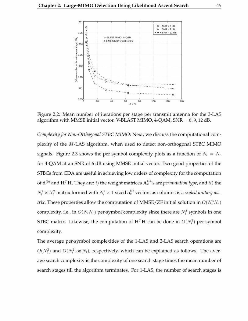
Chapter 2. Large-MIMO Detection Using Likelihood Ascent Search 45
0 20 40 60 80 100 120 1400.05
0.1
0.15
0.2
0.25
0.3
0.35
0.4
(Mea
n nu
mbe
r of
iter
atio
ns p
er s
tage
) / N
t
Nt = Nr
3−LAS, MMSE initial vector
V−BLAST MIMO, 4−QAM
SNR = 6 dBSNR = 9 dBSNR = 12 dB
Figure 2.2: Mean number of iterations per stage per transmit antenna for the 3-LASalgorithm with MMSE initial vector. V-BLAST MIMO, 4-QAM, SNR = 6, 9, 12 dB.
Complexity for Non-Orthogonal STBC MIMO: Next, we discuss the computational com-
plexity of the M-LAS algorithm, when used to detect non-orthogonal STBC MIMO
signals. Figure 2.3 shows the per-symbol complexity plots as a function of Nt = Nr
for 4-QAM at an SNR of 6 dB using MMSE initial vector. Two good properties of the
STBCs from CDA are useful in achieving low orders of complexity for the computation
of d(0) and HTH. They are: i) the weight matrices A(i)c ’s are permutation type, and ii) the
N2t ×N2
t matrix formed with N2t × 1-sized a
(i)c vectors as columns is a scaled unitary ma-
trix. These properties allow the computation of MMSE/ZF initial solution in O(N3t Nr)
complexity, i.e., in O(NtNr) per-symbol complexity since there are N2t symbols in one
STBC matrix. Likewise, the computation of HTH can be done in O(N3t ) per-symbol
complexity.
The average per-symbol complexities of the 1-LAS and 2-LAS search operations are
O(N2t ) and O(N2
t log Nt), respectively, which can be explained as follows. The aver-
age search complexity is the complexity of one search stage times the mean number of
search stages till the algorithm terminates. For 1-LAS, the number of search stages is
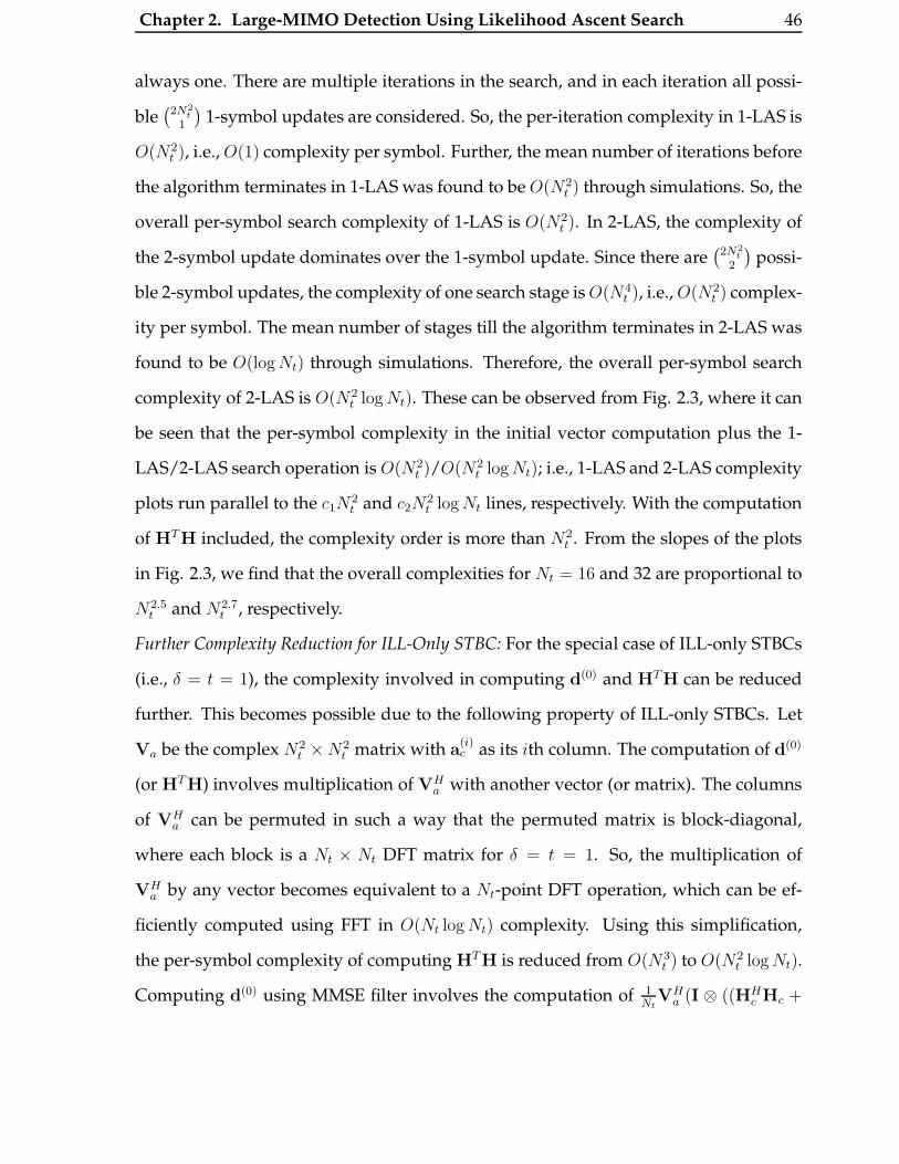
Chapter 2. Large-MIMO Detection Using Likelihood Ascent Search 46
always one. There are multiple iterations in the search, and in each iteration all possi-
ble(2N2
t
1
)1-symbol updates are considered. So, the per-iteration complexity in 1-LAS is
O(N2t ), i.e., O(1) complexity per symbol. Further, the mean number of iterations before
the algorithm terminates in 1-LAS was found to be O(N2t ) through simulations. So, the
overall per-symbol search complexity of 1-LAS is O(N2t ). In 2-LAS, the complexity of
the 2-symbol update dominates over the 1-symbol update. Since there are(2N2
t
2
)possi-
ble 2-symbol updates, the complexity of one search stage is O(N4t ), i.e., O(N2
t ) complex-
ity per symbol. The mean number of stages till the algorithm terminates in 2-LAS was
found to be O(log Nt) through simulations. Therefore, the overall per-symbol search
complexity of 2-LAS is O(N2t log Nt). These can be observed from Fig. 2.3, where it can
be seen that the per-symbol complexity in the initial vector computation plus the 1-
LAS/2-LAS search operation is O(N2t )/O(N2
t log Nt); i.e., 1-LAS and 2-LAS complexity
plots run parallel to the c1N2t and c2N
2t log Nt lines, respectively. With the computation
of HTH included, the complexity order is more than N2t . From the slopes of the plots
in Fig. 2.3, we find that the overall complexities for Nt = 16 and 32 are proportional to
N2.5t and N2.7
t , respectively.
Further Complexity Reduction for ILL-Only STBC: For the special case of ILL-only STBCs
(i.e., δ = t = 1), the complexity involved in computing d(0) and HTH can be reduced
further. This becomes possible due to the following property of ILL-only STBCs. Let
Va be the complex N2t ×N2
t matrix with a(i)c as its ith column. The computation of d(0)
(or HTH) involves multiplication of VHa with another vector (or matrix). The columns
of VHa can be permuted in such a way that the permuted matrix is block-diagonal,
where each block is a Nt × Nt DFT matrix for δ = t = 1. So, the multiplication of
VHa by any vector becomes equivalent to a Nt-point DFT operation, which can be ef-
ficiently computed using FFT in O(Nt log Nt) complexity. Using this simplification,
the per-symbol complexity of computing HTH is reduced from O(N3t ) to O(N2
t log Nt).
Computing d(0) using MMSE filter involves the computation of 1Nt
VHa (I ⊗ ((HH
c Hc +
Chapter 2. Large-MIMO Detection Using Likelihood Ascent Search 47
2 3 4 5 6 7 85
10
15
20
25
30
log2(N
t)
log 2(N
umbe
r of
ope
ratio
ns p
er s
ymbo
l)
c
1 N
t2
c2 N
t2log(N
t)
c3 N
t3
d(0), HTH, search (1−LAS)
d(0), HTH, search (2−LAS)
d(0), search (1−LAS)
d(0), search (2−LAS)
SNR = 6 dB
Figure 2.3: Computational complexity of the M-LAS algorithm in decoding non-orthogonal STBCs from CDA. MMSE initial vector, 4-QAM, SNR = 6 dB.
1γNt
I)−1HHc ))yc. The complexity of computing the vector (I⊗ ((HH
c Hc + 1γNt
I)−1HHc ))yc
is O(N2t Nr), and the complexity of computing VH
a (I ⊗ ((HHc Hc + 1
γNtI)−1HH
c ))yc is
O(N3t Nr). In the case of ILL-only STBC, because of the above-mentioned property, the
complexity of computing VHa (I⊗((HH
c Hc+1
γNtI)−1HH
c ))yc gets reduced to O(N2t log Nt)
from O(N3t Nr). So the total complexity for computing d(0) in ILL-only STBC is O(N2
t Nr)+
O(N2t log Nt), which gives a per-symbol complexity of O(Nr)+O(log Nt). So, the overall
per-symbol complexity for 1-LAS detection of ILL-STBCs is O(N2t log Nt).
2.2.5 Generation of Soft Outputs
We propose to generate soft values at the M-LAS output for all the individual bits
that constitute theM-PAM/M-QAM symbols as follows. The method is described for
STBC MIMO, but is applicable for V-BLAST MIMO as well. These output values are
fed as soft inputs to the decoder in a coded system. Let d = [x1, x2, · · · , x2N2t], xi ∈ Ai
denote the detected output symbol vector from the M-LAS algorithm. Let the symbol
xi map to the bit vector bi = [bi,1, bi,2, · · · , bi,Ki]T , where Ki = log2 |Ai|, and bi,j ∈ {+1,−1},

Chapter 2. Large-MIMO Detection Using Likelihood Ascent Search 48
i = 1, 2, · · · , 2N2t and j = 1, 2, · · · ,Ki. Let bi,j ∈ R denote the soft value for the jth bit of
the ith symbol. Given d, we need to find bi,j, ∀ (i, j).
Note that the quantity ‖y−Hd‖2 is inversely related to the likelihood that d is indeed
the transmitted symbol vector. Let the d vector with its jth bit of the ith symbol forced
to +1 be denoted as vector dj+i . Likewise, let d
j−i be the vector d with its jth bit of
the ith symbol forced to -1. Then the quantities ‖y − Hdj+i ‖2 and ‖y − Hd
j−i ‖2 are
inversely related to the likelihoods that the jth bit of the ith transmitted symbol is +1
and -1, respectively. So, if ‖y−Hdj−i ‖2−‖y−Hd
j+i ‖2 is +ve (or -ve), it indicates that the
jth bit of the ith transmitted symbol has a higher likelihood of being +1 (or -1). So, the
quantity ‖y −Hdj−i ‖2 − ‖y −Hd
j+i ‖2, appropriately normalized to avoid unbounded
increase for increasing Nt, can be a good soft value for the jth bit of the ith symbol.
With this motivation, we generate the soft output value for the jth bit of the ith symbol
as
bi,j =‖y −Hd
j−i ‖2 − ‖y −Hd
j+i ‖2
‖hi‖2, (2.41)
where the normalization by ‖hi‖2 is to contain unbounded increase of bi,j for increasing
Nt. The RHS in the above can be efficiently computed in terms of z and G as follows.
Since dj+i and d
j−i differ only in the ith entry, we can write
dj−i = d
j+i + λi,jei. (2.42)
Since we know dj−i and d
j+i , we know λi,j from (2.42). Substituting (2.42) in (2.41), we
can write
bi,j ‖hi‖2 = ‖y−Hdj+i − λi,jhi‖2 − ‖y−Hd
j+i ‖2
= λ2
i,j‖hi‖2 − 2λi,jhTi (y −Hd
j+i ) (2.43)
= −λ2
i,j‖hi‖2 − 2λi,jhTi (y −Hd
j−i ). (2.44)

Chapter 2. Large-MIMO Detection Using Likelihood Ascent Search 49
If bi,j = 1, then dj+i = d and substituting this in (2.43) and dividing by ‖hi‖2, we get
bi,j = λ2
i,j − 2λi,jzi
(G)i,i. (2.45)
If bi,j = −1, then dj−i = d and substituting this in (2.44) and dividing by ‖hi‖2, we get
bi,j = −λ2
i,j − 2λi,jzi
(G)i,i
. (2.46)
It is noted that z and G are already available upon the termination of the M-LAS al-
gorithm, and hence the complexity of computing bi,j in (2.45) and (2.46) is constant.
Hence, the overall complexity in computing the soft values for all the bits is O(Nt log2M).
We also see from (2.45) and (2.46) that the magnitude of bi,j depends upon λi,j . For
large-size signal sets, the possible values of λi,j will also be large in magnitude. We
therefore have to normalize bi,j for the turbo decoder to function properly. It has been
observed through simulations that normalizing bi,j by(λi,j
2
)2resulted in good perfor-
mance.
2.3 Performance in Large V-BLAST MIMO
In this section, we report uncoded and coded BER performance of the M-LAS detector
for V-BLAST MIMO systems.
Uncoded BER Performance: In Fig. 2.4, we present the uncoded BER of 3-LAS detector
for different values of Nt = Nr and 4-QAM, obtained through simulations. MMSE filter
is used as the initial filter. MMSE filter performance without subsequent LAS search
is also plotted for comparison. As we mentioned earlier, we use the BER performance
in SISO unfaded AWGN channel as a lower bound for comparison. It is observed that
the BER performance of 3-LAS improves with increasing Nr = Nt. For e.g., at an un-
coded BER of 10−3, with Nr = Nt = 16, the performance of 3-LAS is about 3 dB away
from SISO AWGN performance, whereas with Nr = Nt = 256, the performance gets

Chapter 2. Large-MIMO Detection Using Likelihood Ascent Search 50
0 2 4 6 8 10 1210
−5
10−4
10−3
10−2
10−1
100
Average Received SNR (dB)
Bit
Err
or R
ate
V−BLAST MIMO, 4−QAM3−LAS, MMSE initial vector
BER performance improves withincreasing Nt = Nr
Nt = Nr = 16, 3−LASNt = Nr = 32, 3−LASNt = Nr = 64, 3−LASNt = Nr = 64, MMSE−onlyNt = Nr = 128, 3−LASNt = Nr = 256, 3−LASSISO AWGN
Figure 2.4: Uncoded BER performance of 3-LAS detection for different values of Nt =Nr = (16, 32, 64, 128, 256) and 4-QAM. MMSE initial filter.
close to within just 0.4 dB from the SISO AWGN performance. We refer to this be-
havior as ’large-system behavior’ of the LAS algorithm. We observed that MMSE-only
performance without subsequent LAS search do not improve for increasing Nt = Nr.
Therefore, the proposed LAS search is found to be an effective mechanism to improve
upon the performance of the initial MMSE solution at the same order of complexity as
that of the MMSE solution.
In Fig. 2.5, we plot the SNR required to achieve a target BER of 10−3 with 1-LAS de-
tector for increasing Nt = Nr and 4-QAM. MMSE initial vector is used. It is observed
that, the SNR required to meet the target BER indeed gets closer to the SISO AWGN
SNR for increasing Nt = Nr. It is interesting to see that 1-LAS performance is far from
SISO AWGN performance for small values of Nr = Nt. Therefore, in a way, large di-
mensions are actually favorable for the convergence of the LAS algorithm to the correct
transmitted vector. A similar large-system behavior is observed with 16-QAM as well,
which is illustrated in Fig. 2.6.
Next, in Fig. 2.7, we compare the performance of 1-LAS and 3-LAS detection for
Nt = Nr = 64, 32 and 4-QAM. It can be seen that 3-LAS outperforms 1-LAS. This

Chapter 2. Large-MIMO Detection Using Likelihood Ascent Search 51
100
101
102
103
8
10
12
14
16
18
20
22
24
26
28
Number of antennas, Nt = Nr
Ave
rage
rec
eive
d S
NR
req
uire
d (d
B)
1−LAS
SISO AWGN
Near SISO AWGNPerformance
V−BLAST MIMO, 4−QAMNt = Nr, MMSE initial vector
Target BER = 10−3
Figure 2.5: Average received SNR required to achieve a target BER of 10−3 in V-BLASTMIMO for increasing values of Nt = Nr using 1-LAS detection with MMSE initialvector. 4-QAM.
100
101
102
103
104
15
20
25
30
35
40
45
50
Number of antennas, Nt = Nr
Ave
rage
rec
eive
d S
NR
req
uire
d (d
B)
1−LAS SISO AWGN
Target BER = 10−4
V−BLAST MIMO, 16−QAMNt = Nr, MMSE initial vector
Figure 2.6: Average received SNR required to achieve a target BER of 10−4 in V-BLASTMIMO for increasing values of Nt = Nr using 1-LAS detection with MMSE initialvector. 16-QAM.
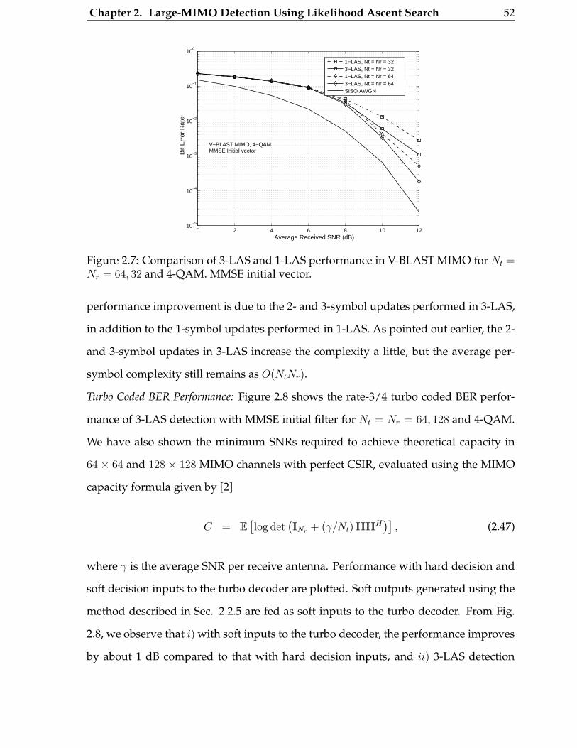
Chapter 2. Large-MIMO Detection Using Likelihood Ascent Search 52
0 2 4 6 8 10 1210
−5
10−4
10−3
10−2
10−1
100
Average Received SNR (dB)
Bit
Err
or R
ate
V−BLAST MIMO, 4−QAMMMSE Initial vector
1−LAS, Nt = Nr = 323−LAS, Nt = Nr = 321−LAS, Nt = Nr = 643−LAS, Nt = Nr = 64SISO AWGN
Figure 2.7: Comparison of 3-LAS and 1-LAS performance in V-BLAST MIMO for Nt =Nr = 64, 32 and 4-QAM. MMSE initial vector.
performance improvement is due to the 2- and 3-symbol updates performed in 3-LAS,
in addition to the 1-symbol updates performed in 1-LAS. As pointed out earlier, the 2-
and 3-symbol updates in 3-LAS increase the complexity a little, but the average per-
symbol complexity still remains as O(NtNr).
Turbo Coded BER Performance: Figure 2.8 shows the rate-3/4 turbo coded BER perfor-
mance of 3-LAS detection with MMSE initial filter for Nt = Nr = 64, 128 and 4-QAM.
We have also shown the minimum SNRs required to achieve theoretical capacity in
64 × 64 and 128 × 128 MIMO channels with perfect CSIR, evaluated using the MIMO
capacity formula given by [2]
C = E[log det
(INr + (γ/Nt)HHH
)], (2.47)
where γ is the average SNR per receive antenna. Performance with hard decision and
soft decision inputs to the turbo decoder are plotted. Soft outputs generated using the
method described in Sec. 2.2.5 are fed as soft inputs to the turbo decoder. From Fig.
2.8, we observe that i) with soft inputs to the turbo decoder, the performance improves
by about 1 dB compared to that with hard decision inputs, and ii) 3-LAS detection

Chapter 2. Large-MIMO Detection Using Likelihood Ascent Search 53
−2 0 2 4 6 8 10 12 14 1610
−4
10−3
10−2
10−1
100
Average Received SNR (dB)
Bit
Err
or R
ate
V−BLAST MIMO, 4−QAM Rate−3/4 Turbo Code
Min. SNR required to achieve capacity
Min
. SN
R =
4.3
dB
3−LAS, Nr = N
t = 64 (Hard input)
3−LAS, Nr = N
t = 64 (Soft input)
3−LAS, Nr = N
t = 128 (Hard input)
3−LAS, Nr = N
t = 128 (Soft input)
Figure 2.8: Turbo coded BER performance of 3-LAS detection for Nt = Nr = 64, 128,4-QAM, and rate-3/4 turbo code. MMSE initial vector.
achieves a coded performance (i.e., vertical fall in coded BER) which is close to within
about 4.5 dB from theoretical capacity.
2.4 Performance in Large Non-orthogonal STBC MIMO
In this section, we present the uncoded/turbo coded BER performance of the M-LAS
detector in decoding non-orthogonal STBCs from CDA, assuming perfect knowledge
of CSIR2. In all the BER simulations in this section, we have assumed that the fade
remains constant over one STBC matrix duration and varies i.i.d. from one STBC ma-
trix duration to the other. We consider two STBC designs; i) ‘FD-ILL’ STBCs where
δ = e√
5 j, t = ej in (2.15), and ii) ‘ILL-only’ STBCs where δ = t = 1. The SNRs in
all the BER performance figures are the average received SNR per received antenna,
γ, defined in Section 2.1.4 [2]. We have used MMSE filter as the initial filter in all the
simulations.
2We will relax this perfect channel knowledge assumption in the next section, where we present aniterative detection/channel estimation scheme for the considered large STBC MIMO system.

Chapter 2. Large-MIMO Detection Using Likelihood Ascent Search 54
2 4 6 8 10 12 1410
−6
10−5
10−4
10−3
10−2
10−1
100
Average Received SNR (dB)
Bit
Err
or R
ate
ILL−only STBCs, 4−QAM Nr = Nt, 2Nt bps/Hz
(1) : 4x4 STBC, MMSE−only
(2) : 8x8 STBC, MMSE−only
(3) : 16x16 STBC, MMSE−only
(4) : 32x32 STBC, MMSE−only
4x4 STBC, 1−LAS
8x8 STBC, 1−LAS
16x16 STBC, 1−LAS
(5) : 32x32 STBC, 1−LAS
4x4 STBC, 2−LAS
8x8 STBC, 2−LAS
16x16 STBC, 2−LAS
(6) : 32x32 STBC, 2−LAS
4x4 STBC, 3−LAS
8x8 STBC, 3−LAS
SISO AWGN
(5, 6)
BER improves withincreasing Nr =Nt.
MMSE−only (No LAS)(1, 2, 3, 4)
Figure 2.9: Uncoded BER performance of 1-LAS, 2-LAS and 3-LAS detectors for ILL-only STBCs for different Nt = Nr. 4-QAM, 2Nt bps/Hz.
2.4.1 Uncoded BER as a Function of Increasing Nt = Nr
In Fig. 2.9, we plot the uncoded BER performance of the 1-, 2-, and 3-LAS algorithms in
decoding ILL-only STBCs (4× 4, 8× 8, 16× 16, 32× 32 STBCs) for Nt = Nr = 4, 8, 16, 32
and 4-QAM. SISO AWGN performance (without fading) and MMSE-only performance
(i.e., without the search using LAS) are also plotted for comparison. It can be seen that
MMSE-only performance does not improve with increasing STBC size (i.e., increasing
Nt = Nr). However, it is interesting to see that, when the proposed search using LAS
is performed following the MMSE operation, the performance improves for increas-
ing Nt = Nr, illustrating the performance benefit due to the proposed search strategy.
For example, though the LAS detector performs far from SISO AWGN performance
for small number of dimensions (e.g., 4 × 4, 8 × 8 STBCs with 32 and 128 real dimen-
sions, respectively), its large system behavior at increased number of dimensions (e.g.,
16× 16 and 32× 32 STBCs with 512 and 2048 real dimensions, respectively) effectively
renders near SISO AWGN performance; e.g., with Nt = Nr = 16, 32, for BERs better
than 10−3, the LAS detector performs very close to SISO AWGN performance. We also
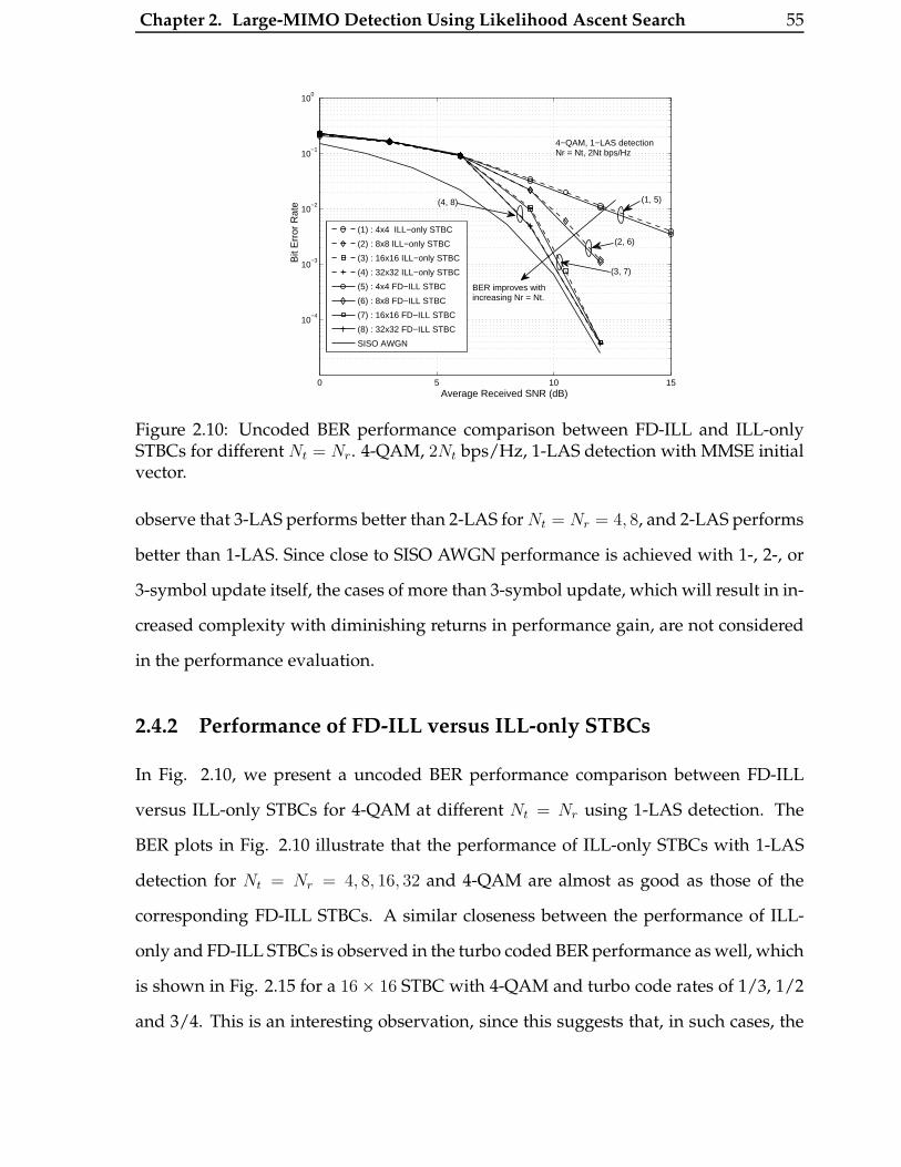
Chapter 2. Large-MIMO Detection Using Likelihood Ascent Search 55
0 5 10 15
10−4
10−3
10−2
10−1
100
Average Received SNR (dB)
Bit
Err
or R
ate
(1, 5)
BER improves withincreasing Nr = Nt.
4−QAM, 1−LAS detectionNr = Nt, 2Nt bps/Hz
(1) : 4x4 ILL−only STBC
(2) : 8x8 ILL−only STBC
(3) : 16x16 ILL−only STBC
(4) : 32x32 ILL−only STBC
(5) : 4x4 FD−ILL STBC
(6) : 8x8 FD−ILL STBC
(7) : 16x16 FD−ILL STBC
(8) : 32x32 FD−ILL STBC
SISO AWGN
(2, 6)
(3, 7)
(4, 8)
Figure 2.10: Uncoded BER performance comparison between FD-ILL and ILL-onlySTBCs for different Nt = Nr. 4-QAM, 2Nt bps/Hz, 1-LAS detection with MMSE initialvector.
observe that 3-LAS performs better than 2-LAS for Nt = Nr = 4, 8, and 2-LAS performs
better than 1-LAS. Since close to SISO AWGN performance is achieved with 1-, 2-, or
3-symbol update itself, the cases of more than 3-symbol update, which will result in in-
creased complexity with diminishing returns in performance gain, are not considered
in the performance evaluation.
2.4.2 Performance of FD-ILL versus ILL-only STBCs
In Fig. 2.10, we present a uncoded BER performance comparison between FD-ILL
versus ILL-only STBCs for 4-QAM at different Nt = Nr using 1-LAS detection. The
BER plots in Fig. 2.10 illustrate that the performance of ILL-only STBCs with 1-LAS
detection for Nt = Nr = 4, 8, 16, 32 and 4-QAM are almost as good as those of the
corresponding FD-ILL STBCs. A similar closeness between the performance of ILL-
only and FD-ILL STBCs is observed in the turbo coded BER performance as well, which
is shown in Fig. 2.15 for a 16× 16 STBC with 4-QAM and turbo code rates of 1/3, 1/2
and 3/4. This is an interesting observation, since this suggests that, in such cases, the
Chapter 2. Large-MIMO Detection Using Likelihood Ascent Search 56
computational complexity advantage with δ = t = 1 in ILL-only STBCs can be taken
advantage of without incurring much performance loss compared to FD-ILL STBCs.
2.4.3 Decoding and BER of Perfect Codes of Large Dimensions
While the STBC design in (2.15) offers both ILL and FD, perfect codes3 under ML decod-
ing can provide coding gain in addition to ILL and FD [84]-[22]. Decoding of perfect
codes has been reported in the literature for only up to 5 antennas using sphere/lattice
decoding [87]. The complexity of these decoders are prohibitive for decoding large-
sized perfect codes, although large-sized codes are of interest from a high spectral ef-
ficiency view point. We note that, because of its low-complexity attribute, the M-LAS
detector is able to decode perfect codes of large dimensions. In Figs. 2.11 and 2.12, we
present the simulated BER performance of perfect codes in comparison with those of
ILL-only and FD-ILL STBCs for up to 32 transmit antennas using 1-LAS detector.
In Fig. 2.11, we show uncoded BER comparison between perfect codes and ILL-only
STBCs for different Nt = Nr and 4-QAM using 1-LAS detection. The 4 × 4 and 6 × 6
perfect codes are from [86], and the 8×8, 16×16 and 32×32 perfect codes are from [87].
From Fig. 2.11, it can be seen that the 1-LAS detector achieves better performance for
ILL-only STBCs than for perfect codes, when codes with small number of transmit an-
tennas are considered (e.g., Nt = 4, 6, 8). While perfect codes are expected to perform
better than ILL-only codes under ML detection for any Nt, we observe the opposite be-
havior under 1-LAS detection for small Nt (i.e., ILL-only STBCs performing better than
perfect codes for small dimensions). This behavior could be attributed to the nature of
the LAS detector, which achieves near-optimal performance only when the number of
dimensions is large, and it appears that, in the detection process, LAS is more effective
in disentangling the symbols in STBCs when δ = t = 1 (i.e., in ILL-only STBCs) than in
3We note that the definition of perfect codes differ in [86] and [87]. The perfect codes covered bythe definition in [87] includes the perfect codes of [86] as a proper subclass. However, for our purposeof illustrating the performance of the proposed detector in large STBC MIMO systems, we refer to thecodes in [86] as well as [87] as perfect codes.

Chapter 2. Large-MIMO Detection Using Likelihood Ascent Search 57
0 5 10 15 20 25 3010
−5
10−4
10−3
10−2
10−1
100
Average Received SNR (dB)
Bit
Err
or R
ate
4x4 Perfect code6x6 Perfect code8x8 Perfect code(1): 16x16 Perfect code(2): 32x32 Perfect code4x4 ILL−only STBC6x6 ILL−only STBC8x8 ILL−only STBC(3): 16x16 ILL−only STBC(4): 32x32 ILL−only STBCSISO AWGN
(1, 3)
(2, 4)
4−QAM, 1−LAS detectionNt = Nr, 2Nt bps/Hz
Figure 2.11: Uncoded BER comparison between perfect codes and ILL-only STBCs fordifferent Nt = Nr, 4-QAM, 2Nt bps/Hz, 1-LAS detection.
perfect codes. The performance gap between perfect codes and ILL-only STBCs with
1-LAS detection diminishes for increasing code sizes such that the performance for
32× 32 perfect code and ILL-only STBC with 4-QAM are almost same and close to the
SISO AWGN performance. In Fig. 2.12, we show a similar comparison between perfect
codes, ILL-only and FD-ILL only STBCs when larger modulation alphabet sizes (e.g.,
16-QAM) are used in the case of 16 × 16 and 32 × 32 codes. It can be seen that with
higher-order QAM like 16-QAM, perfect codes with 1-LAS detection perform poorer
than ILL-only and FD-ILL STBCs, and that ILL-only and FD-ILL STBCs perform al-
most same and close to the SISO AWGN performance. The results in Figs. 2.11 and
2.12 suggest that, with 1-LAS detection, owing to the complexity advantage and good
performance in using δ = t = 1, ILL-only STBCs can be a good choice for practical
large STBC MIMO systems [109],[110].

Chapter 2. Large-MIMO Detection Using Likelihood Ascent Search 58
5 10 15 20 25 30 35 40 4510
−5
10−4
10−3
10−2
10−1
100
Average Received SNR (dB)
Bit
Err
or R
ate
16x16 Perfect code(1) : 16x16 ILL−only STBC(2) : 16x16 FD−ILL STBC32x32 Perfect code(3) : 32x32 ILL−only STBC(4) : 32x32 FD−ILL STBCSISO AWGN
(1, 2)
(3, 4)
16−QAM, 1−LAS detection Nr = Nt, 4Nt bps/Hz.
Figure 2.12: Uncoded BER performance comparison between perfect codes, ILL-only,and FD-ILL STBCs for Nt = Nr = 16, 32, 16-QAM, 4Nt bps/Hz, 1-LAS detection.
2.4.4 Comparison with Other Large-MIMO Architecture/Detector
Combinations
In [111], Choi et al have presented an iterative soft interference cancellation (ISIC)
scheme for multiple antenna systems, derived based on maximum a posteriori (MAP)
criterion. We compared the performance of the ISIC scheme in [111] with that of the
1-LAS algorithm in detecting 4×4, 8×8 and 16×16 ILL-only STBCs with Nt = Nr and
4-QAM. Figure 2.13 shows this performance comparison. In [111], zero-forcing vec-
tor was used as the initial vector in the ISIC scheme. However, performance is better
with MMSE initial vector. Since we used MMSE initial vector for 1-LAS, we have used
MMSE initial vector for the ISIC algorithm as well. Also, in [111], 4 to 5 iterations were
shown to be good enough for the ISIC algorithm to converge. In our simulations of
the ISIC algorithm, we used 10 iterations. Two key observations can be made from Fig.
2.13: i) like the 1-LAS algorithm, the ISIC algorithm also shows large system behavior
(i.e., improved BER for increasing Nt = Nr), and 2) the 1-LAS algorithm outperforms
the ISIC algorithm by about 3 to 5 dB at 10−3 uncoded BER. In addition, the complexity

Chapter 2. Large-MIMO Detection Using Likelihood Ascent Search 59
0 5 10 15 20 2510
−5
10−4
10−3
10−2
10−1
100
101
Average Received SNR (dB)
Bit
Err
or R
ate
4x4 ILL−only STBC, ISIC (Choi et al [111])
8x8 ILL−only STBC, ISIC (Choi et al [111])
16x16 ILL−only STBC, ISIC (Choi et al [111])
4x4 ILL−only STBC, 1−LAS (Proposed)
8x8 ILL−only STBC, 1−LAS (Proposed)
16x16 ILL−only STBC, 1−LAS (Proposed)
SISO AWGN
Nt = Nr, 4−QAM, 2Nt bps/Hz10 iterations in ISIC
Figure 2.13: Uncoded BER performance comparison between the 1-LAS algorithm andthe ISIC algorithm in [111] for ILL-only STBCs for different Nt = Nr. 4-QAM, 2Nt
bps/Hz. MMSE initial vectors for both 1-LAS and ISIC.
of the ISIC scheme is higher than the proposed scheme (see the complexity comparison
in Table 2.1).
Next, we compare the proposed large-MIMO architecture using STBCs from CDA and
M-LAS detection with other large-MIMO architectures and associated detectors re-
ported in the literature. Large-MIMO architectures that use stacking of multiple small-
sized STBCs and interference cancellation (IC) detectors for these schemes have been
investigated in [88],[112],[113]. Here, we compare different architecture/detector com-
binations, fixing the total number of transmit/receive antennas and spectral efficiency
to be same in all the considered combinations. Specifically, we fix Nt = Nr = 16 and
a spectral efficiency of 32 bps/Hz for all the combinations. We compare the following
seven different architecture/detector combinations which use the same Nt = Nr = 16
and achieve 32 bps/Hz spectral efficiency (see Table 2.1): i) proposed scheme using
16× 16 ILL-only STBC (rate-16) with 4-QAM and 1-LAS detection, ii) 16× 16 ILL-only
STBC (rate-16) with 4-QAM and ISIC algorithm in [111] with 10 iterations, iii) four
4× 4 stacked QOSTBCs (rate-1) with 256-QAM and IC algorithm presented in [88], iv)
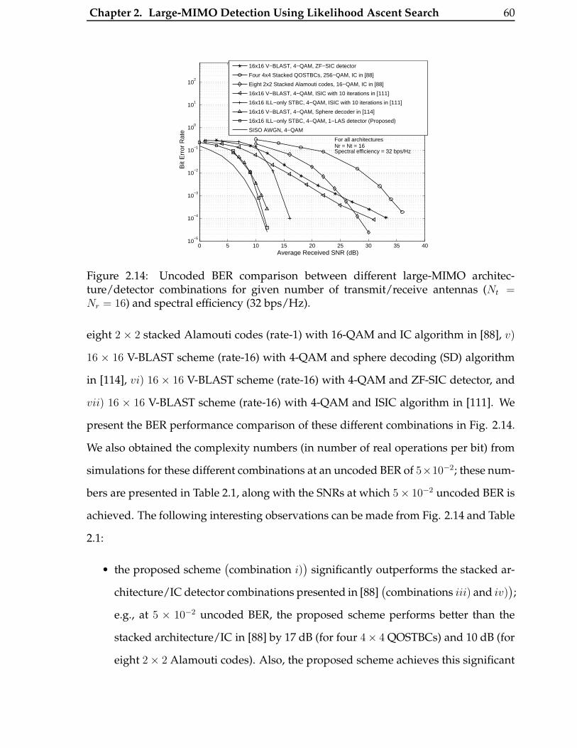
Chapter 2. Large-MIMO Detection Using Likelihood Ascent Search 60
0 5 10 15 20 25 30 35 4010
−5
10−4
10−3
10−2
10−1
100
101
102
Average Received SNR (dB)
Bit
Err
or R
ate
16x16 V−BLAST, 4−QAM, ZF−SIC detector
Four 4x4 Stacked QOSTBCs, 256−QAM, IC in [88]
Eight 2x2 Stacked Alamouti codes, 16−QAM, IC in [88]
16x16 V−BLAST, 4−QAM, ISIC with 10 iterations in [111]
16x16 ILL−only STBC, 4−QAM, ISIC with 10 iterations in [111]
16x16 V−BLAST, 4−QAM, Sphere decoder in [114]
16x16 ILL−only STBC, 4−QAM, 1−LAS detector (Proposed)
SISO AWGN, 4−QAM
For all architecturesNr = Nt = 16Spectral efficiency = 32 bps/Hz
Figure 2.14: Uncoded BER comparison between different large-MIMO architec-ture/detector combinations for given number of transmit/receive antennas (Nt =Nr = 16) and spectral efficiency (32 bps/Hz).
eight 2 × 2 stacked Alamouti codes (rate-1) with 16-QAM and IC algorithm in [88], v)
16 × 16 V-BLAST scheme (rate-16) with 4-QAM and sphere decoding (SD) algorithm
in [114], vi) 16 × 16 V-BLAST scheme (rate-16) with 4-QAM and ZF-SIC detector, and
vii) 16 × 16 V-BLAST scheme (rate-16) with 4-QAM and ISIC algorithm in [111]. We
present the BER performance comparison of these different combinations in Fig. 2.14.
We also obtained the complexity numbers (in number of real operations per bit) from
simulations for these different combinations at an uncoded BER of 5×10⁻²; these num-
bers are presented in Table 2.1, along with the SNRs at which 5× 10⁻² uncoded BER is
achieved. The following interesting observations can be made from Fig. 2.14 and Table
2.1:
• the proposed scheme(combination i)
)significantly outperforms the stacked ar-
chitecture/IC detector combinations presented in [88](combinations iii) and iv)
);
e.g., at 5 × 10⁻² uncoded BER, the proposed scheme performs better than the
stacked architecture/IC in [88] by 17 dB (for four 4× 4 QOSTBCs) and 10 dB (for
eight 2× 2 Alamouti codes). Also, the proposed scheme achieves this significant
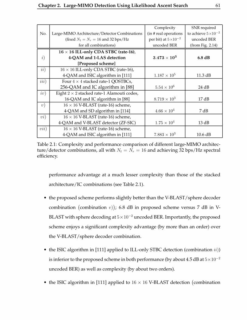
Chapter 2. Large-MIMO Detection Using Likelihood Ascent Search 61
Complexity SNR required
No. Large-MIMO Architecture/Detector Combinations (in # real operations to achieve 5×10⁻²
(fixed Nt = Nr = 16 and 32 bps/Hz per bit) at 5×10⁻² uncoded BER
for all combinations) uncoded BER (from Fig. 2.14)
16× 16 ILL-only CDA STBC (rate-16),
i) 4-QAM and 1-LAS detection 3.473 × 10³ 6.8 dB
[Proposed scheme]
ii) 16× 16 ILL-only CDA STBC (rate-16),
4-QAM and ISIC algorithm in [111] 1.187 × 10⁵ 11.3 dB
iii) Four 4× 4 stacked rate-1 QOSTBCs,
256-QAM and IC algorithm in [88] 5.54 × 10⁶ 24 dB
iv) Eight 2× 2 stacked rate-1 Alamouti codes,
16-QAM and IC algorithm in [88] 8.719 × 10³ 17 dB
v) 16× 16 V-BLAST (rate-16) scheme,
4-QAM and SD algorithm in [114] 4.66 × 10⁴ 7 dB
vi) 16× 16 V-BLAST (rate-16) scheme,
4-QAM and V-BLAST detector (ZF-SIC) 1.75 × 10⁴ 13 dB
vii) 16× 16 V-BLAST (rate-16) scheme,
4-QAM and ISIC algorithm in [111] 7.883 × 10³ 10.6 dB
Table 2.1: Complexity and performance comparison of different large-MIMO architec-ture/detector combinations, all with Nt = Nr = 16 and achieving 32 bps/Hz spectralefficiency.
performance advantage at a much lesser complexity than those of the stacked
architecture/IC combinations (see Table 2.1).
• the proposed scheme performs slightly better than the V-BLAST/sphere decoder
combination(combination v)
); 6.8 dB in proposed scheme versus 7 dB in V-
BLAST with sphere decoding at 5×10⁻² uncoded BER. Importantly, the proposed
scheme enjoys a significant complexity advantage (by more than an order) over
the V-BLAST/sphere decoder combination.
• the ISIC algorithm in [111] applied to ILL-only STBC detection (combination ii))
is inferior to the proposed scheme in both performance (by about 4.5 dB at 5×10⁻²
uncoded BER) as well as complexity (by about two orders).
• the ISIC algorithm in [111] applied to 16 × 16 V-BLAST detection(combination
Chapter 2. Large-MIMO Detection Using Likelihood Ascent Search 62
vii))
is also inferior to the proposed scheme in BER performance (by about 3.8 dB
at 5× 10⁻² uncoded BER) as well as complexity (by about a factor of 2).
• comparing the stacked architecture/IC combinations with V-BLAST/ZF-SIC(co-
mbination vi))
and V-BLAST/ISIC combinations, we see that although the diver-
sity orders achieved in stacked architecture/IC combinations are high (see their
slopes at high SNRs in Fig. 2.14), V-BLAST with ZF-SIC and ISIC detectors per-
form much better at low and medium SNRs.
In summary, the proposed scheme outperforms the other considered architecture/de-
tector combinations both in terms of performance as well as complexity.
2.4.5 Turbo Coded BER and Nearness-to-Capacity Results
Turbo Coded BER performance : Fast Fading Channel
We discuss the turbo coded BER performance of the proposed scheme when the MIMO
channel is assumed to be quasi-static (i.e., for a (n, p, k) non-orthogonal STBC, the
MIMO channel is static for p channel uses, and changes to an independent realiza-
tion for the next p channel uses). In all the coded BER simulations, we fed the soft
outputs presented in Sec. 2.2.5 as input to the turbo decoder. In Fig. 2.15, we plot
the turbo coded BER of the 1-LAS detector in decoding 16 × 16 FD-ILL and ILL-only
STBCs, with Nt = Nr = 16, 4-QAM and turbo code rates 1/3 (10.6 bps/Hz), 1/2 (16
bps/Hz), 3/4 (24 bps/Hz). The minimum SNRs required to achieve these capacities in
a 16 × 16 MIMO channel (obtained by evaluating the ergodic MIMO capacity expres-
sion in [5] through simulation) are also shown. It can be seen that the 1-LAS detector
performs close to within just about 4 dB from capacity, which is very good in terms of
nearness-to-capacity considering the high spectral efficiencies achieved. It can also be
seen that the coded BER performance of FD-ILL and ILL-only STBCs are almost the
same for the system parameters considered. Figure 2.16 shows the turbo coded BER

Chapter 2. Large-MIMO Detection Using Likelihood Ascent Search 63
−2 0 2 4 6 8 10 12 14 16 18
10−4
10−3
10−2
10−1
100
Average Received SNR (dB)
Bit
Err
or R
ate
16x16 STBCs, 4−QAMNr = Nt = 16, 1−LAS detection
Min
SN
R =
−1.
45 d
B
Min
SN
R =
1.2
dB
Min
SN
R =
4.3
dB
(1) : Rate−1/3 turbo (ILL−Only STBC)
(2) : Rate−1/2 turbo (ILL−Only STBC)
(3) : Rate−3/4 turbo (ILL−Only STBC)
(4) : Rate−1/3 turbo (FD−ILL STBC)
(5) : Rate−1/2 turbo (FD−ILL STBC)
(6) : Rate−3/4 turbo (FD−ILL STBC)
Min SNR for capacity = 10.6 b/s/Hz
Min SNR for capacity = 16 b/s/Hz
Min SNR for capacity = 24 b/s/Hz
(2, 5)
(1, 4)
(3, 6)
Figure 2.15: Turbo coded BER performance of 1-LAS detector for 16 × 16 FD-ILL andILL-only STBCs. Nt = Nr = 16, 4-QAM, turbo code rates: 1/3, 1/2, 3/4 (10.6, 16, 24bps/Hz).
performance of 32 × 32 ILL-only STBC with Nt = Nr = 32, 16-QAM, and turbo code
rates 1/3 (42.6 bps/Hz), 1/2 (64 bps/Hz), 3/4 (96 bps/Hz) using 1-LAS detection.
Turbo Coded BER Performance: Slow Fading Channel
We next discuss the turbo coded performance of the proposed 1-LAS detector in a slow
fading channel, where the MIMO channel is static for the full duration of the turbo
coded frame, and changes to an independent realization in the next turbo frame. Fig-
ure 2.17 shows the rate-3/4 turbo coded performance of 1-LAS detection with MMSE
initial filter for Nr = Nt = (4, 8, 12) and 4-QAM. FD-ILL STBCs are used in order to
achieve the full diversity gain of the MIMO channel. The target spectral efficiency is
1.5Nt bps/Hz. The MIMO channel outage probability (given by (1.3)), which is the
theoretical limit for the codeword error probability (CEP) of long codewords, is also
plotted for the sake of comparison. It is observed that, 1-LAS search improves the
codeword error probability significantly when compared to the error performance of
the MMSE-only initial detector. At a CEP of 10−2, MMSE 1-LAS performs better than
the MMSE-only detector by about 2.5 dB for Nr = Nt = 8, 12. Further, with increasing

Chapter 2. Large-MIMO Detection Using Likelihood Ascent Search 64
0 5 10 15 20 25 3010
−5
10−4
10−3
10−2
10−1
100
Average Received SNR (dB)
Bit
Err
or R
ate
Rate−1/3 turboRate−1/2 turbo Rate−3/4 turboMin SNR for capacity = 42.6 bps/HzMin SNR for capacity = 64 bps/HzMin SNR for capacity = 96 bps/Hz
Min
SN
R =
6.8
3 dB
Min
SN
R =
11.
12 d
B
32 x 32 ILL−only STBCNt = Nr = 32, 16−QAMSoft LAS outputs
Min
SN
R =
3.3
2 dB
Figure 2.16: Turbo coded BER performance of 1-LAS detector for 32 × 32 ILL-onlySTBC. Nt = Nr = 32, 16-QAM, turbo code rates: 1/3, 1/2, 3/4 (42.6, 64, 96 bps/Hz).
−5 0 5 10 15 2010
−3
10−2
10−1
100
Average Received SNR (dB)
Cod
ewor
d E
rror
Rat
e
Nr = N
t = 4 (MMSE−only)
Nr = N
t = 4 (MMSE 1−LAS)
Nr = N
t = 4 (MIMO outage)
Nr = N
t = 8 (MMSE−only)
Nr = N
t = 8 (MMSE 1−LAS)
Nr = N
t = 8 (MIMO outage)
Nr = N
t = 12 (MMSE−only)
Nr = N
t = 12 (MMSE 1−LAS)
Nr = N
t = 12 (MIMO outage)
MIMO Slow Fading, Nr = N
t, 4−QAM
Transmission Rate = 1.5Nt bps/Hz
Rate−3/4 Turbo code. Nt X N
t FD−ILL STBC
Figure 2.17: Turbo codeword error probability of 1-LAS detection in a slow fadingMIMO channel for Nt = Nr = 4, 8, 12, 4-QAM, rate-3/4 turbo code and FD-ILL STBCs.MMSE initial vector.
Chapter 2. Large-MIMO Detection Using Likelihood Ascent Search 65
Nr = Nt, the error performance of MMSE 1-LAS is observed to improve and achieve a
higher diversity slope. This is similar to the ‘large-system behavior’ observed for the
uncoded BER performance of the LAS detector. The MMSE 1-LAS detector is also ob-
served to perform close to the theoretical outage probability of the MIMO channel. At
a CEP of 10−2, the MMSE 1-LAS detector performs within 4.5 dB of the MIMO channel
outage probability for Nr = Nt = 12.
2.4.6 Effect of MIMO Spatial Correlation
In generating the BER results in Figs. 2.9 to 2.16, we have assumed i.i.d. fading. How-
ever, MIMO propagation conditions witnessed in practice often render the i.i.d. fading
model as inadequate. More realistic MIMO channel models that take into account the
scattering environment, spatial correlation, etc., have been investigated in the litera-
ture [8],[9]. For example, spatial correlation at the transmit and/or receive side can
affect the rank structure of the MIMO channel resulting in degraded MIMO capac-
ity [9]. The structure of scattering in the propagation environment can also affect the
capacity [8]. Hence, it is of interest to investigate the performance of the M-LAS detec-
tor in more realistic MIMO channel models. To this end, we use the non-line-of-sight
(NLOS) correlated MIMO channel model proposed by Gesbert et al in [8], and evaluate
the effect of spatial correlation on the BER performance of the M-LAS detector. We note
that this model can be appropriate in application scenarios like high data rate wireless
IPTV/HDTV distribution using high spectral efficiency large-MIMO links, where large
Nt and Nr can be placed at the base station (BS) and customer premises equipment
(CPE), respectively. The propagation scenario for the MIMO channel model consid-
ered is shown in Fig. 2.18, where linear arrays of Nt omnidirectional transmit antennas
with spacing dt, and Nr omnidirectional receive antennas with spacing dr are consid-
ered [8]. The propagation path between the transmit and receive arrays is obstructed
on both sides of the link by a number of significant near-field scatterers (e.g., large

Chapter 2. Large-MIMO Detection Using Likelihood Ascent Search 66
objects) referred to as transmit and receive scatterers, which are modeled as omnidi-
rectional ideal scatterers. The maximum range of the scatterers from the horizontal
axis at the transmit and receive sides are denoted by Dt and Dr, respectively. When
omnidirectional antennas are used, Dt and Dr correspond to the transmit and receive
scattering radii, respectively. On the receive side, the signal reflected by the scatterers
onto the antennas impinge on the array with an angular spread θr, which is a function
of the distance between the array and the scatterers. Similarly, angular spread θt is de-
fined on the transmit side. The range between the local scatterers at the transmit and
receive sides is denoted by R. It is assumed that the scatterers are located adequately
far from the antennas so that the plane-wave assumption holds. Further, local scatter-
ing condition is assumed, i.e., Dt << R and Dr << R. The number of scatterers on
each side, S, is considered to be large enough (typically > 10) for random fading to
occur. The complex channel gain matrix as per this model is given by [8]
Hc =1√S
R1/2θr,dr
GrR1/2θS ,2Dr/SGtR
1/2θt,dt
, (2.48)
where Gt = [g1g2 · · ·gNt ] is an S × Nt i.i.d. Rayleigh fading matrix, gn ∼ CN (0, IS),
Gr = [g1g2 · · ·gNr ], R1/2θt,dt
and R1/2θr ,dr
are the Nt×Nt and Nr×Nr matrices controlling the
transmit and receive antenna correlations, respectively, whose expressions are given in
[8].
We consider the following parameters4 in the simulations: fc = 5 GHz, R = 500 m,
S = 30, Dt = Dr = 20 m, θt = θr = 90◦, and dt = dr = 2λ/3. For fc = 5 GHz, λ = 6 cm
and dt = dr = 4 cm. In Fig. 2.14, we plot the BER performance of the 1-LAS detector
in decoding 16 × 16 ILL-only STBC with Nt = Nr = 16 and 16-QAM. Uncoded BER
as well as rate-3/4 turbo coded BER (48 bps/Hz spectral efficiency) for i.i.d. fading
4The parameters used in the model in [8] include: Nt, Nr : # transmit and receive (omni-directional)antennas; dt, dr: spacing between antenna elements at the transmit side and at the receive side; R:distance between transmitter and receiver, Dt, Dr: transmit and receive scattering radii; S: numberof scatterers on each side; θt, θr: angular spread at the transmit and receiver sides, and fc, λ: carrierfrequency, wavelength.

Chapter 2. Large-MIMO Detection Using Likelihood Ascent Search 67
NtTXs
dt
θt
Dt
R
θs
Dr
θr
NrRXs
dr
Figure 2.18: Propagation scenario for the MIMO fading channel model.
as well as correlated fading are shown. In addition, from the MIMO capacity formula
in [5], we evaluated the theoretical minimum SNRs required to achieve a capacity of
48 bps/Hz in i.i.d. as well as correlated fading, and plotted them also in Fig. 2.14.
It is seen that the minimum SNR required to achieve a certain capacity (48 bps/Hz)
gets increased for correlated fading compared to i.i.d. fading. From the BER plots
in Fig. 2.14, it can be observed that at an uncoded BER of 10−3, the performance in
correlated fading degrades by about 7 dB compared that in i.i.d. fading. Likewise, at
a rate-3/4 turbo coded BER of 10−4, a performance loss of about 6 dB is observed in
correlated fading compared to that in i.i.d. fading. In terms of nearness to capacity,
the vertical fall of the coded BER for i.i.d. fading occurs at about 24 dB SNR, which is
about 13 dB away from theoretical minimum required SNR of 11.1 dB. With correlated
fading, the detector is observed to perform close to capacity within about 18.5 dB. One
way to alleviate such degradation in performance due to spatial correlation can be by
providing more number of dimensions at the receive side, which is highlighted in Fig.
2.19.
Figure 2.19 illustrates that the 1-LAS detector can achieve substantial improvement
in uncoded as well as coded BER performance in decoding 12 × 12 ILL-only STBC
by increasing Nr beyond Nt for 16-QAM in correlated fading. In the simulations,
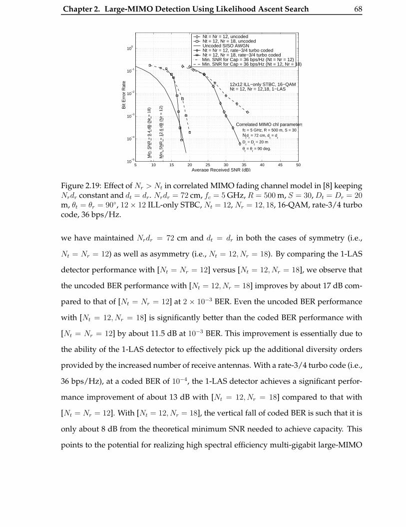
Chapter 2. Large-MIMO Detection Using Likelihood Ascent Search 68
5 10 15 20 25 30 35 40 45 5010
−5
10−4
10−3
10−2
10−1
100
Average Received SNR (dB)
Bit
Err
or R
ate
Nt = Nr = 12, uncodedNt = 12, Nr = 18, uncodedUncoded SISO AWGNNt = Nr = 12, rate−3/4 turbo codedNt = 12, Nr = 18, rate−3/4 turbo codedMin. SNR for Cap = 36 bps/Hz (Nt = Nr = 12)Min. SNR for Cap = 36 bps/Hz (Nt = 12, Nr = 18)
12x12 ILL−only STBC, 16−QAMNt = 12, Nr = 12,18, 1−LAS
Correlated MIMO chl parameters:
Nrd
r = 72 cm, d
t = d
r
Dr = D
t = 20 m
fc = 5 GHz, R = 500 m, S = 30
θt = θ
r = 90 deg.
Min
. SN
R =
12.
6 dB
(N
r =
12)
Min
. SN
R =
9.4
dB
(N
r =
18)
Figure 2.19: Effect of Nr > Nt in correlated MIMO fading channel model in [8] keepingNrdr constant and dt = dr. Nrdr = 72 cm, fc = 5 GHz, R = 500 m, S = 30, Dt = Dr = 20m, θt = θr = 90◦, 12× 12 ILL-only STBC, Nt = 12, Nr = 12, 18, 16-QAM, rate-3/4 turbocode, 36 bps/Hz.
we have maintained Nrdr = 72 cm and dt = dr in both the cases of symmetry (i.e.,
Nt = Nr = 12) as well as asymmetry (i.e., Nt = 12, Nr = 18). By comparing the 1-LAS
detector performance with [Nt = Nr = 12] versus [Nt = 12, Nr = 18], we observe that
the uncoded BER performance with [Nt = 12, Nr = 18] improves by about 17 dB com-
pared to that of [Nt = Nr = 12] at 2 × 10⁻³ BER. Even the uncoded BER performance
with [Nt = 12, Nr = 18] is significantly better than the coded BER performance with
[Nt = Nr = 12] by about 11.5 dB at 10−3 BER. This improvement is essentially due to
the ability of the 1-LAS detector to effectively pick up the additional diversity orders
provided by the increased number of receive antennas. With a rate-3/4 turbo code (i.e.,
36 bps/Hz), at a coded BER of 10−4, the 1-LAS detector achieves a significant perfor-
mance improvement of about 13 dB with [Nt = 12, Nr = 18] compared to that with
[Nt = Nr = 12]. With [Nt = 12, Nr = 18], the vertical fall of coded BER is such that it is
only about 8 dB from the theoretical minimum SNR needed to achieve capacity. This
points to the potential for realizing high spectral efficiency multi-gigabit large-MIMO

Chapter 2. Large-MIMO Detection Using Likelihood Ascent Search 69
systems that can achieve good performance even in the presence of spatial correla-
tion. We further remark that transmit correlation in MIMO fading can be exploited
by using non-isotropic inputs (precoding) based on the knowledge of the channel
correlation matrices [10]-[12]. While [10]-[12] propose precoders in conjunction with
orthogonal/quasi-orthogonal small MIMO systems in correlated Rayleigh/Ricean fad-
ing, design of precoders for large-MIMO systems can be investigated as future work.
2.5 Iterative Detection/Channel Estimation
In this section, we relax the perfect CSIR assumption made in the previous section,
and estimate the channel matrix based on a training-based iterative detection/channel
estimation scheme. Training-based schemes, where a pilot signal known to the trans-
mitter and the receiver is sent to get a rough estimate of the channel (training phase)
has been studied for STBC MIMO systems in [115]-[118]. Here, we adopt a training-
based approach for channel estimation in large STBC MIMO systems. In the consid-
ered training-based channel estimation scheme, transmission is carried out in frames,
where one Nt × Nt pilot matrix, X(P)c ∈ C
Nt×Nt , for training purposes, followed by
Nd data STBC matrices, X(i)c ∈ CNt×Nt, i = 1, 2, ..., Nd, are sent in each frame as
shown in Fig. 2.20. One frame length, T , (taken to be the channel coherence time)
is T = (Nd + 1)Nt channel uses. A frame of transmitted pilot and data matrices is of
dimension Nt ×Nt(1 + Nd), which can be written as
Xc =[X(P)
c X(1)c X(2)
c · · ·X(Nd)c
]. (2.49)
As in [119], let γp and γd denote the average SNR during pilot and data phases, re-
spectively, which are related to the average received SNR γ as γ(Nd + 1) = γp + Ndγd.
Define βp4= γp
γ, and βd
4= γd
γ. Let Es denote the average energy of the transmitted
symbol during the data phase. The average received signal power during the data

Chapter 2. Large-MIMO Detection Using Likelihood Ascent Search 70
phase is given by E[tr(X
(i)c X
(i)c
H)]= N2
t Es, and the average received signal power
during the pilot phase is E[tr(X
(P)c X
(P)c
H)]=
N2t Esβp
βd= µNt, where µ
4= NtEsβp
βd. For
optimal training, the pilot matrix should be such that X(P)c X(P)
cH
= µINt [119]. As in
Section 2.1.2, let Hc ∈ CNr×Nt denote the channel matrix, which we want to estimate.
We assume block fading, where the channel gains remain constant over one frame
consisting of (1 + Nd)Nt channel uses, which can be viewed as the channel coherence
time. This assumption can be valid in slow fading fixed wireless applications (e.g., as
in possible applications like BS-to-BS backbone connectivity and BS-to-CPE wireless
IPTV/HDTV distribution). For this training-based system and channel model, Hassibi
and Hochwald presented a lower bound on the capacity in [119]; we will illustrate the
nearness of the performance achieved by the proposed iterative detection/estimation
scheme to this bound. The received frame is of dimension Nr ×Nt(1 + Nd), and can be
written as
Yc =[Y(P)
c Y(1)c Y(2)
c · · ·Y(Nd)c
]= HcXc +Nc , (2.50)
whereNc =[N(P)
c N(1)c N
(2)c · · ·N(Nd)
c
]is the Nr×Nt(1+Nd) noise matrix and its entries
are modeled as i.i.d. CN (0, σ2 = NtEs
γβd). Equation (2.50) can be decomposed into two
parts, namely, the pilot matrix part and the data matrices part, as
Y(P)c = HcX
(P)c + N(P)
c , (2.51)
Y(D)c =
[Y(1)
c Y(2)c · · ·Y(Nd)
c
]
= Hc
[X(1)
c X(2)c · · ·X(Nd)
c
]+[N(1)
c N(2)c · · ·N(Nd)
c
]. (2.52)
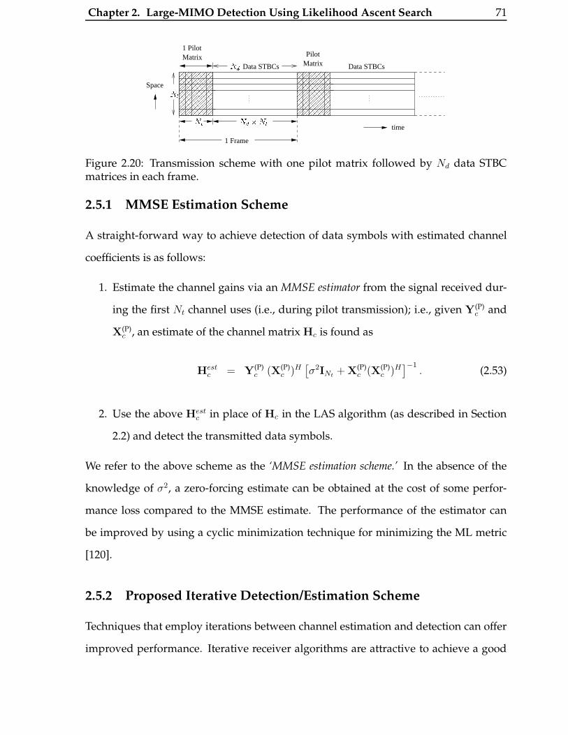
Chapter 2. Large-MIMO Detection Using Likelihood Ascent Search 71
������
����������������
��������������������
����������������������������
��������
��������������������
��������������������������������������������
��������
����
���
���
��
���
���
��
����
��������
��������
time
Data STBCs
Space
MatrixMatrixPilot
1 Pilot
Data STBCs
1 Frame
Nt Nt Nd �NtNd
Figure 2.20: Transmission scheme with one pilot matrix followed by Nd data STBCmatrices in each frame.
2.5.1 MMSE Estimation Scheme
A straight-forward way to achieve detection of data symbols with estimated channel
coefficients is as follows:
1. Estimate the channel gains via an MMSE estimator from the signal received dur-
ing the first Nt channel uses (i.e., during pilot transmission); i.e., given Y(P)c and
X(P)c , an estimate of the channel matrix Hc is found as
Hestc = Y(P)
c (X(P)c )H
[σ2INt + X(P)
c (X(P)c )H
]−1. (2.53)
2. Use the above Hestc in place of Hc in the LAS algorithm (as described in Section
2.2) and detect the transmitted data symbols.
We refer to the above scheme as the ‘MMSE estimation scheme.’ In the absence of the
knowledge of σ2, a zero-forcing estimate can be obtained at the cost of some perfor-
mance loss compared to the MMSE estimate. The performance of the estimator can
be improved by using a cyclic minimization technique for minimizing the ML metric
[120].
2.5.2 Proposed Iterative Detection/Estimation Scheme
Techniques that employ iterations between channel estimation and detection can offer
improved performance. Iterative receiver algorithms are attractive to achieve a good
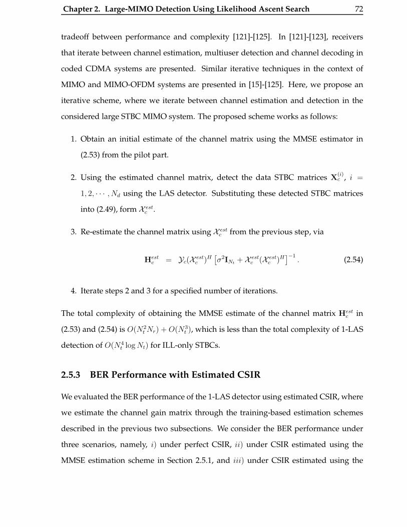
Chapter 2. Large-MIMO Detection Using Likelihood Ascent Search 72
tradeoff between performance and complexity [121]-[125]. In [121]-[123], receivers
that iterate between channel estimation, multiuser detection and channel decoding in
coded CDMA systems are presented. Similar iterative techniques in the context of
MIMO and MIMO-OFDM systems are presented in [15]-[125]. Here, we propose an
iterative scheme, where we iterate between channel estimation and detection in the
considered large STBC MIMO system. The proposed scheme works as follows:
1. Obtain an initial estimate of the channel matrix using the MMSE estimator in
(2.53) from the pilot part.
2. Using the estimated channel matrix, detect the data STBC matrices X(i)c , i =
1, 2, · · · , Nd using the LAS detector. Substituting these detected STBC matrices
into (2.49), form X estc .
3. Re-estimate the channel matrix using X estc from the previous step, via
Hestc = Yc(X est
c )H[σ2INt + X est
c (X estc )H
]−1. (2.54)
4. Iterate steps 2 and 3 for a specified number of iterations.
The total complexity of obtaining the MMSE estimate of the channel matrix Hestc in
(2.53) and (2.54) is O(N2t Nr) + O(N3
t ), which is less than the total complexity of 1-LAS
detection of O(N4t log Nt) for ILL-only STBCs.
2.5.3 BER Performance with Estimated CSIR
We evaluated the BER performance of the 1-LAS detector using estimated CSIR, where
we estimate the channel gain matrix through the training-based estimation schemes
described in the previous two subsections. We consider the BER performance under
three scenarios, namely, i) under perfect CSIR, ii) under CSIR estimated using the
MMSE estimation scheme in Section 2.5.1, and iii) under CSIR estimated using the

Chapter 2. Large-MIMO Detection Using Likelihood Ascent Search 73
−4 −2 0 2 4 6 8 10 12 14 160
10
20
30
40
50
60
70
Average SNR (dB)
Erg
od
ic C
ap
acity (
bp
s/H
z)
Perfect CSIR1P + 8D (H−H bound)1P + 1D (H−H bound)
16 x 16 MIMO Channel
24 bps/Hz21.3 bps/Hz
12 bps/Hz
7.7
dB
4.3
dB
Figure 2.21: Hassibi-Hochwald (H-H) capacity bound for 1P+8D (T = 144, τ = 16, βp =βd = 1) and 1P+1D (T = 32, τ = 16, βp = βd = 1) training for a 16× 16 MIMO channel.Perfect CSIR capacity is also shown.
iterative detection/estimation scheme in Section 2.5.2. In the case of estimated CSIR,
we show plots for 1P+NdD training, where by 1P+NdD training we mean a training
scheme with a frame size of 1 + Nd matrices, with 1 pilot matrix followed Nd data
STBC matrices from CDA. For this 1P+NdD training scheme, a lower bound on the
capacity is given by [119]
C ≥ T − τ
TE
[logdet
(INt +
γ2βdβpτ
Nt(1 + γβd) + γβpτ
HcHHc
Ntσ2Hc
)], (2.55)
where T and τ , respectively, are the frame size (i.e., channel coherence time) and pi-
lot duration in number of channel uses, and σ2Hc
= 1NtNr
E[tr{HcH
Hc }], where Hc =
E[Hc
∣∣ X(P)c ,Y(P)
c
]is the MMSE estimate of the channel gain matrix. We computed
the capacity bound in (2.55) through simulations for 1P+8D and 1P+1D training for a
16×16 MIMO channel. For 1P+8D training T = (1+8)16 = 144, τ = 16, and for 1P+1D
training T = (1 + 1)16 = 32, τ = 16. In computing the bounds (shown in Fig. 2.21) and
in BER simulations (in Figs. 2.22 and 2.23), we have used βp = βd = 1. In Fig. 2.21,
we plot the computed capacity bounds, along with the capacity under perfect CSIR
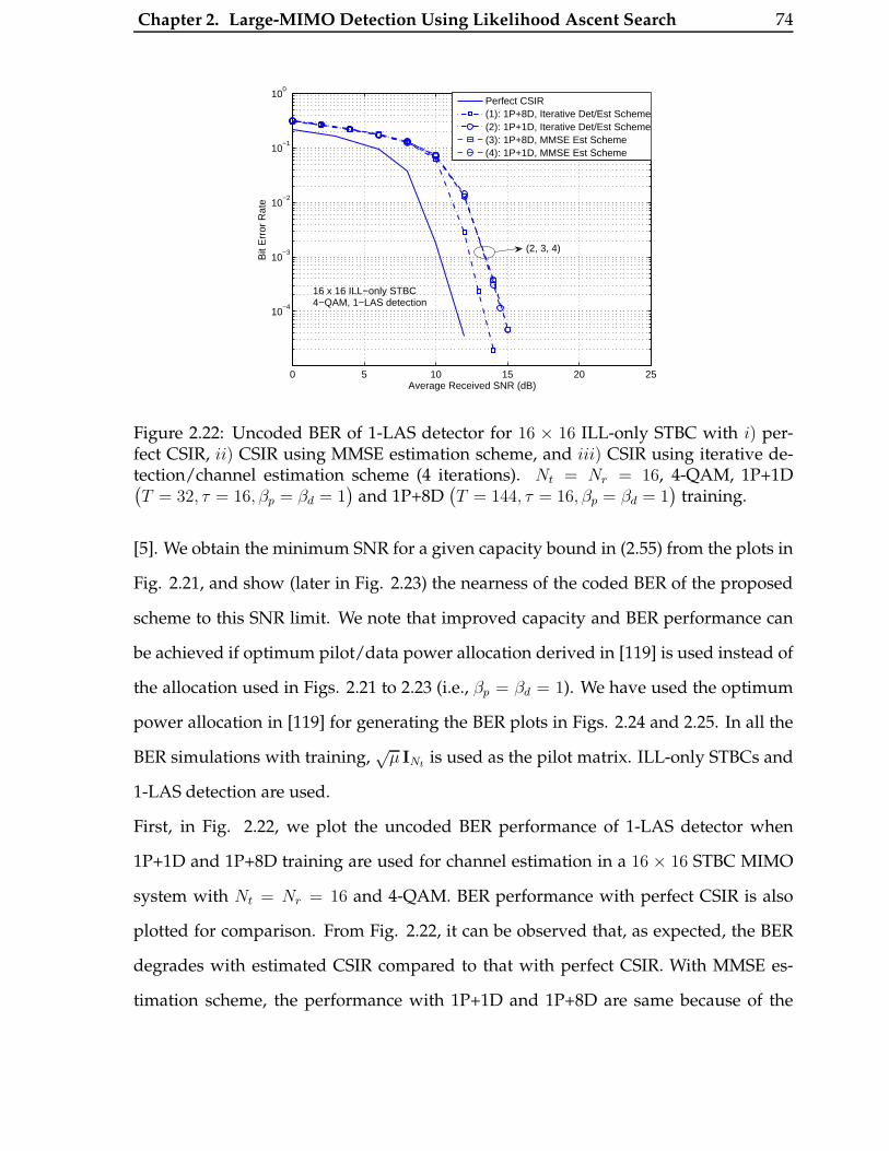
Chapter 2. Large-MIMO Detection Using Likelihood Ascent Search 74
0 5 10 15 20 25
10−4
10−3
10−2
10−1
100
Average Received SNR (dB)
Bit
Err
or R
ate
Perfect CSIR(1): 1P+8D, Iterative Det/Est Scheme(2): 1P+1D, Iterative Det/Est Scheme(3): 1P+8D, MMSE Est Scheme(4): 1P+1D, MMSE Est Scheme
16 x 16 ILL−only STBC4−QAM, 1−LAS detection
(2, 3, 4)
Figure 2.22: Uncoded BER of 1-LAS detector for 16 × 16 ILL-only STBC with i) per-fect CSIR, ii) CSIR using MMSE estimation scheme, and iii) CSIR using iterative de-tection/channel estimation scheme (4 iterations). Nt = Nr = 16, 4-QAM, 1P+1D(T = 32, τ = 16, βp = βd = 1
)and 1P+8D
(T = 144, τ = 16, βp = βd = 1
)training.
[5]. We obtain the minimum SNR for a given capacity bound in (2.55) from the plots in
Fig. 2.21, and show (later in Fig. 2.23) the nearness of the coded BER of the proposed
scheme to this SNR limit. We note that improved capacity and BER performance can
be achieved if optimum pilot/data power allocation derived in [119] is used instead of
the allocation used in Figs. 2.21 to 2.23 (i.e., βp = βd = 1). We have used the optimum
power allocation in [119] for generating the BER plots in Figs. 2.24 and 2.25. In all the
BER simulations with training,√
µ INt is used as the pilot matrix. ILL-only STBCs and
1-LAS detection are used.
First, in Fig. 2.22, we plot the uncoded BER performance of 1-LAS detector when
1P+1D and 1P+8D training are used for channel estimation in a 16 × 16 STBC MIMO
system with Nt = Nr = 16 and 4-QAM. BER performance with perfect CSIR is also
plotted for comparison. From Fig. 2.22, it can be observed that, as expected, the BER
degrades with estimated CSIR compared to that with perfect CSIR. With MMSE es-
timation scheme, the performance with 1P+1D and 1P+8D are same because of the
Chapter 2. Large-MIMO Detection Using Likelihood Ascent Search 75
4 6 8 10 12 14 16 1810
−5
10−4
10−3
10−2
10−1
100
Average Received SNR (dB)
Bit
Err
or R
ate
(1): 1P+1D, Iter Det/EstScheme (4 iterns.)(2): 1P+8D, Iter Det/EstScheme (4 iterns.)(3): 1P+1D, MMSE EstScheme(4): 1P+8D, MMSE EstSchemePerfect CSIR(5): Min SNR; 12 bps/Hzcap. bnd;1P+1D(6): Min SNR; 21.3 bps/Hzcap. bnd;1P+8DMin SNR; 24 bps/Hzcap.;perfect CSIR
16 x 16 ILL−only STBCNt=Nr=16, 4−QAMRate−3/4 turbo code1−LAS detection
4.3
dB
7.7
dB
(1, 3, 4)(5, 6)
Figure 2.23: Turbo coded BER performance of 1-LAS detector for 16×16 ILL-only STBCwith i) perfect CSIR, ii) CSIR using MMSE estimation, and iii) CSIR using iterativedetection/channel estimation (4 iterations). Nt = Nr = 16, 4-QAM, rate-3/4 turbocode, 1P+1D
(T = 32, τ = 16, βp = βd = 1
)and 1P+8D
(T = 144, τ = 16, βp = βd = 1
)
training.
one-shot estimation. Also, with 1P+1D training, both the MMSE estimation scheme
as well as the iterative detection/estimation scheme (with 4 iterations between de-
tection and estimation) perform almost the same, which is about 3 dB worse com-
pared to that of perfect CSIR at an uncoded BER of 10−3. This indicates that with
1P+NdD training, iteration between detection and estimation does not improve per-
formance much over the non-iterative scheme (i.e., the MMSE estimation scheme) for
small Nd. With large Nd (e.g., slow fading), however, the iterative scheme outperforms
the non-iterative scheme; e.g., with 1P+8D training, the performance of the iterative
detection/estimation improves by about 1 dB compared to the MMSE estimation.
Next, in Fig. 2.23, we present the rate-3/4 turbo coded BER of 1-LAS detector using es-
timated CSIR for the cases of 1P+8D and 1P+1D training. From Fig. 2.23, it can be seen
that, compared to that of perfect CSIR, the estimated CSIR performance is worse by
about 3 dB in terms of coded BER for 1P+8D training. With MMSE estimation scheme,
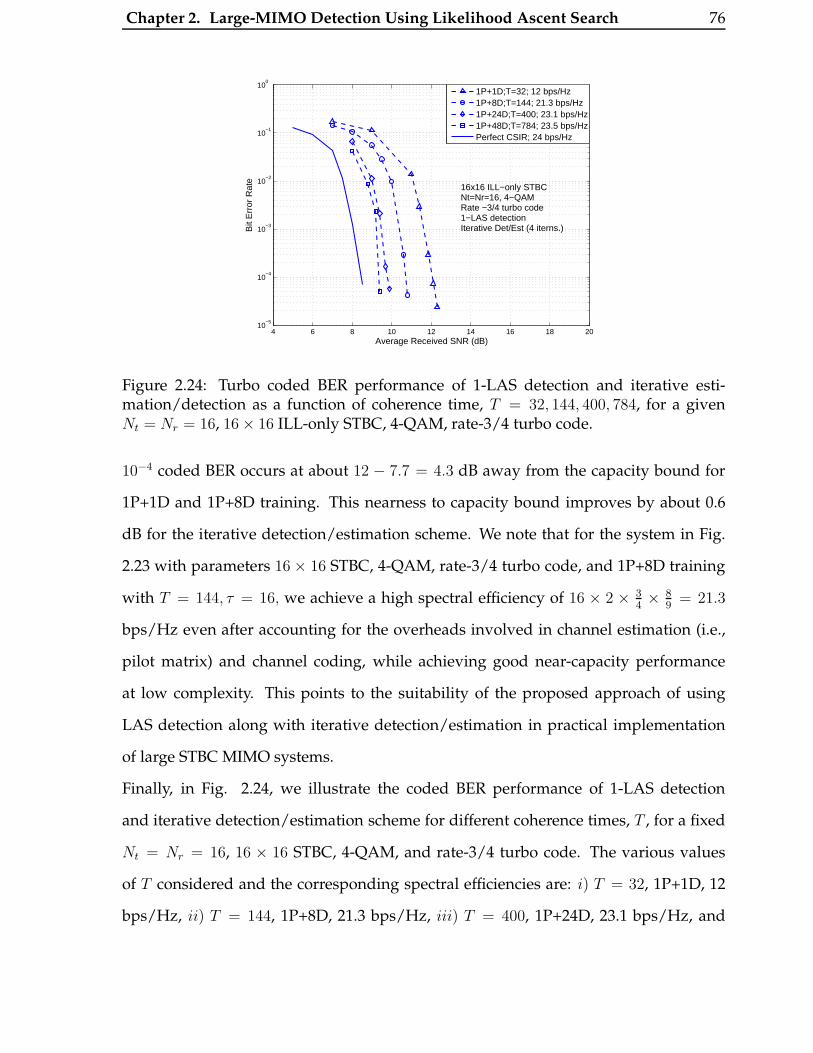
Chapter 2. Large-MIMO Detection Using Likelihood Ascent Search 76
4 6 8 10 12 14 16 18 2010
−5
10−4
10−3
10−2
10−1
100
Average Received SNR (dB)
Bit
Err
or R
ate
1P+1D;T=32; 12 bps/Hz1P+8D;T=144; 21.3 bps/Hz1P+24D;T=400; 23.1 bps/Hz1P+48D;T=784; 23.5 bps/HzPerfect CSIR; 24 bps/Hz
16x16 ILL−only STBCNt=Nr=16, 4−QAMRate −3/4 turbo code1−LAS detectionIterative Det/Est (4 iterns.)
Figure 2.24: Turbo coded BER performance of 1-LAS detection and iterative esti-mation/detection as a function of coherence time, T = 32, 144, 400, 784, for a givenNt = Nr = 16, 16× 16 ILL-only STBC, 4-QAM, rate-3/4 turbo code.
10−4 coded BER occurs at about 12 − 7.7 = 4.3 dB away from the capacity bound for
1P+1D and 1P+8D training. This nearness to capacity bound improves by about 0.6
dB for the iterative detection/estimation scheme. We note that for the system in Fig.
2.23 with parameters 16× 16 STBC, 4-QAM, rate-3/4 turbo code, and 1P+8D training
with T = 144, τ = 16, we achieve a high spectral efficiency of 16 × 2 × 34× 8
9= 21.3
bps/Hz even after accounting for the overheads involved in channel estimation (i.e.,
pilot matrix) and channel coding, while achieving good near-capacity performance
at low complexity. This points to the suitability of the proposed approach of using
LAS detection along with iterative detection/estimation in practical implementation
of large STBC MIMO systems.
Finally, in Fig. 2.24, we illustrate the coded BER performance of 1-LAS detection
and iterative detection/estimation scheme for different coherence times, T , for a fixed
Nt = Nr = 16, 16 × 16 STBC, 4-QAM, and rate-3/4 turbo code. The various values
of T considered and the corresponding spectral efficiencies are: i) T = 32, 1P+1D, 12
bps/Hz, ii) T = 144, 1P+8D, 21.3 bps/Hz, iii) T = 400, 1P+24D, 23.1 bps/Hz, and
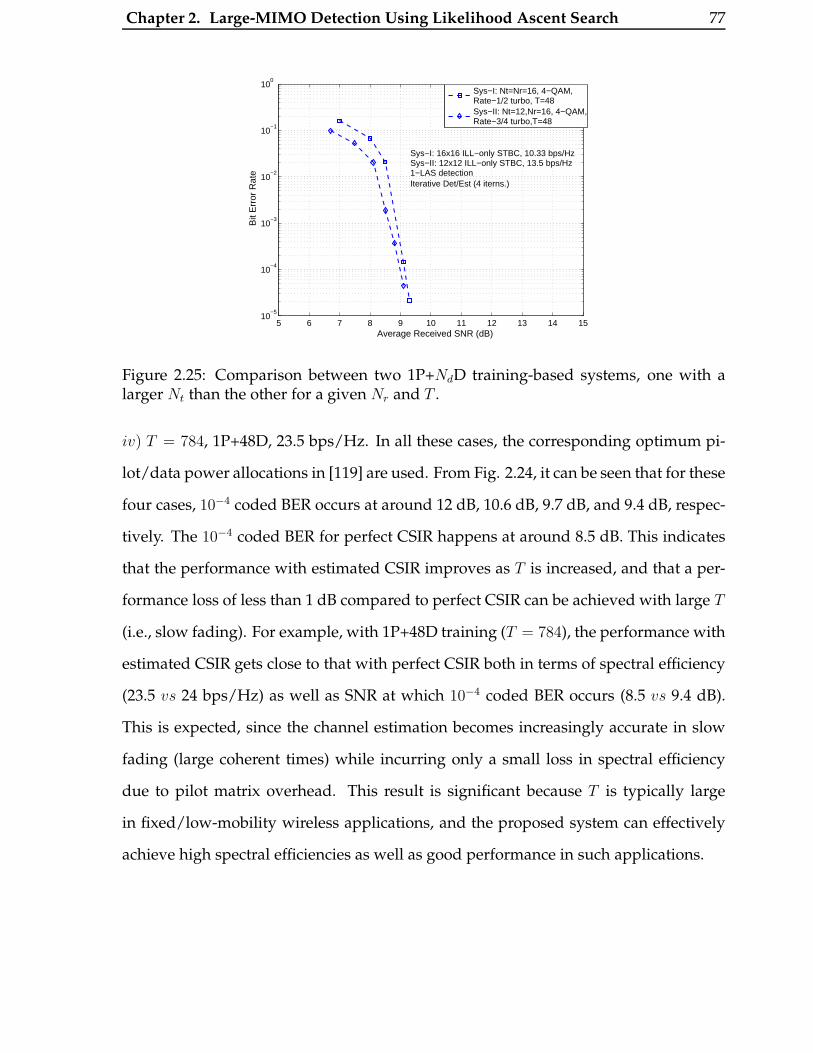
Chapter 2. Large-MIMO Detection Using Likelihood Ascent Search 77
5 6 7 8 9 10 11 12 13 14 1510
−5
10−4
10−3
10−2
10−1
100
Average Received SNR (dB)
Bit
Err
or R
ate
Sys−I: Nt=Nr=16, 4−QAM,Rate−1/2 turbo, T=48Sys−II: Nt=12,Nr=16, 4−QAM,Rate−3/4 turbo,T=48
Sys−I: 16x16 ILL−only STBC, 10.33 bps/HzSys−II: 12x12 ILL−only STBC, 13.5 bps/Hz1−LAS detectionIterative Det/Est (4 iterns.)
Figure 2.25: Comparison between two 1P+NdD training-based systems, one with alarger Nt than the other for a given Nr and T .
iv) T = 784, 1P+48D, 23.5 bps/Hz. In all these cases, the corresponding optimum pi-
lot/data power allocations in [119] are used. From Fig. 2.24, it can be seen that for these
four cases, 10−4 coded BER occurs at around 12 dB, 10.6 dB, 9.7 dB, and 9.4 dB, respec-
tively. The 10−4 coded BER for perfect CSIR happens at around 8.5 dB. This indicates
that the performance with estimated CSIR improves as T is increased, and that a per-
formance loss of less than 1 dB compared to perfect CSIR can be achieved with large T
(i.e., slow fading). For example, with 1P+48D training (T = 784), the performance with
estimated CSIR gets close to that with perfect CSIR both in terms of spectral efficiency
(23.5 vs 24 bps/Hz) as well as SNR at which 10−4 coded BER occurs (8.5 vs 9.4 dB).
This is expected, since the channel estimation becomes increasingly accurate in slow
fading (large coherent times) while incurring only a small loss in spectral efficiency
due to pilot matrix overhead. This result is significant because T is typically large
in fixed/low-mobility wireless applications, and the proposed system can effectively
achieve high spectral efficiencies as well as good performance in such applications.

Chapter 2. Large-MIMO Detection Using Likelihood Ascent Search 78
Parameters System-I System-II
# Rx antennas, Nr 16 16Coherence time, T 48 48# Tx antennas, Nt 16 12STBC from CDA 16× 16 12× 12Pilot duration, τ 16 12Training 1P+2D 1P+3Dβopt
p 1.2426 1.4641βopt
d 0.8786 0.8453Modulation 4-QAM 4-QAMTurbo code rate 1/2 3/4Spectral efficiency 10.33 bps/Hz 13.5 bps/HzSNR at 10−3 coded BER 8.9 dB 8.6 dB
Table 2.2: On optimum Nt for a given Nr and T . System-II with a smaller Nt achieves ahigher spectral efficiency while achieving 10−3 coded BER at a lesser SNR than System-I with a larger Nt.
2.5.4 On Optimum Nt for a Given Nr and T
In [119], through theoretical capacity bounds it has been shown that, for a given Nr, T
and SNR, there is an optimum value of Nt that maximizes the capacity bound(refer
Figs. 5 and 6 in [119], where the optimum Nt is shown to be greater than Nr in Fig.
5 and less than Nr in Fig. 6). For example, for Nr = 16, T = 48, and SNR = 10 dB,
the capacity bound evaluated using (2.55) with optimum power allocation for Nt = 12
is 19.73 bps/Hz, whereas for Nt = 16 the capacity bound reduces to 17.53 bps/Hz
showing that the optimum Nt in this case will be less than Nr. We demonstrate such an
observation in practical systems by comparing the simulated coded BER performance
of two systems, referred to as System-I and System-II, using 1-LAS detection and itera-
tive detection/estimation scheme. The parameters of System-I and System-II are listed
in Table 2.2. Nr and T are fixed at 16 and 48, respectively, in both systems. System-I
uses 16 transmit antennas and 16 × 16 STBC, whereas System-II uses 12 transmit an-
tennas and 12× 12 STBC. Since the pilot matrix is√
µ INt , the pilot duration τ is 16 and
12, respectively, for System-I and System-II. Optimum pilot/data power allocation and
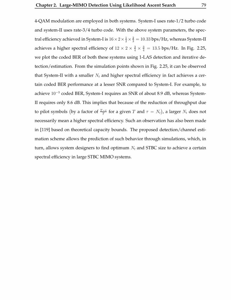
Chapter 2. Large-MIMO Detection Using Likelihood Ascent Search 79
4-QAM modulation are employed in both systems. System-I uses rate-1/2 turbo code
and system-II uses rate-3/4 turbo code. With the above system parameters, the spec-
tral efficiency achieved in System-I is 16×2× 12× 2
3= 10.33 bps/Hz, whereas System-II
achieves a higher spectral efficiency of 12 × 2 × 34× 3
4= 13.5 bps/Hz. In Fig. 2.25,
we plot the coded BER of both these systems using 1-LAS detection and iterative de-
tection/estimation. From the simulation points shown in Fig. 2.25, it can be observed
that System-II with a smaller Nt and higher spectral efficiency in fact achieves a cer-
tain coded BER performance at a lesser SNR compared to System-I. For example, to
achieve 10−3 coded BER, System-I requires an SNR of about 8.9 dB, whereas System-
II requires only 8.6 dB. This implies that because of the reduction of throughput due
to pilot symbols(by a factor of T−τ
Tfor a given T and τ = Nt
), a larger Nt does not
necessarily mean a higher spectral efficiency. Such an observation has also been made
in [119] based on theoretical capacity bounds. The proposed detection/channel esti-
mation scheme allows the prediction of such behavior through simulations, which, in
turn, allows system designers to find optimum Nt and STBC size to achieve a certain
spectral efficiency in large STBC MIMO systems.

Chapter 3
Large-System Performance Analysis of
LAS Algorithm
In Chapter 2, we presented the LAS detection algorithm, and showed through simu-
lations that its error performance improves with increasing Nt = Nr. The BER per-
formance indeed was seen to get increasingly closer to SISO AWGN performance for
increasingly large Nt = Nr at moderate to high SNRs, indicating optimality in the
large-system limit. In this chapter, in an attempt to gain some insights on the large-
system behavior of the algorithm, we carry out an asymptotic performance analysis
of the LAS algorithm in the large-system limit, where Nt → ∞ keeping Nt = Nr. We
present the analysis for a V-BLAST MIMO system, whose real-valued system model
(as described in Chapter 2) is given by
y = Hx + n, (3.1)
where H ∈ R2Nr×2Nt is the equivalent channel matrix, y ∈ R2Nr and x ∈ R2Nt are the
received and transmitted vectors respectively, and n ∈ R2Nr×1 is the additive Gaussian
noise vector. We consider 4-QAM modulation. So, the set of possible input symbols is
S = {+1, −1}2Nt . For a given received vector y and channel realization H, the output
80

Chapter 3. Large-System Performance Analysis of LAS Algorithm 81
of the ML detector is given by
dML =arg min
d ∈ S‖y −Hd‖2 =
arg min
d ∈ S
(dT HTHd− 2yTHd
). (3.2)
3.1 Asymptotic Analysis of the LAS Algorithm
In this section, we analyze the error performance of the LAS algorithm in V-BLAST
MIMO for Nt, Nr →∞, with Nt = Nr and 4-QAM, i.e., S = {+1, −1}2Nt .
An n-symbol update on a data vector d ∈ S transforms d to (d − ∆dn) such that
(d − ∆dn) ∈ S. Further, (d −∆dn) is obtained by changing n symbols in d at distinct
indices given by the n-tuple un4= (i1, i2, · · · , in), 1 ≤ ij ≤ 2Nt,∀j = 1, · · · , n and ij 6=
ik for j 6= k. Therefore, we can write ∆dn as
∆dn =n∑
k=1
2dikeik , (3.3)
where dik is the ikth element of d and eik is a vector with its ikth entry only as one and
all other entries as zero. Let Ln ⊆ S denote the set of data vectors such that for any
d ∈ Ln, if a n-symbol update is performed on d resulting in a vector (d − ∆dn), then
‖y −H(d−∆dn)‖ ≥ ‖y −Hd‖.
Lemma 1. Let d ∈ S. Then, d ∈ Ln if and only if, for any n-update on d, n ∈ [1, 2 · · · , 2Nt],
(y −Hd +
1
2H∆dn
)T (H∆dn
)≥ 0. (3.4)
Proof: By definition, if d ∈ Ln, then no n-symbol update can result in a reduction in the
ML cost function. Using this, we can write
‖y−H(d−∆dn)‖2 ≥ ‖y−Hd‖2. (3.5)
Simplifying (3.5), we get (3.4). Since the choice of the indices in un is arbitrary, the

Chapter 3. Large-System Performance Analysis of LAS Algorithm 82
lemma holds true for all possible n-tuples of distinct indices. For the converse, if d
satisfies (3.4) for all possible un for a given n, then, since (3.4) and (3.5) are equivalent,
d also satisfies (3.5) for all possible un. This implies that d ∈ Ln. �
If d ∈ L1, then using Lemma 1 and (3.1), we can write
(n + H(x− d) + hpdp
)T (hpdp) ≥ 0, ∀p = 1, · · · , 2Nt, (3.6)
where hp is the pth column of H.
Lemma 2. Assuming uniqueness of the ML vector dML in (3.2), a symbol vector d ∈ S is the
ML vector if and only if the noise vector n satisfies the following set of equations
(n + H(x− d) +
( n∑
j=1
hijdij
))T( n∑
j=1
hijdij
)≥ 0, (3.7)
∀n = 1, · · · , 2Nt, and for all possible n-tuples (i1, · · · , in) for each n.
Proof: If d is the unique ML vector, then from the definition of the ML criterion in
(3.2), it must be true that any n-update on d will not result in any decrease in the ML
cost function. Therefore, d ∈ Ln, ∀ n = 1, 2 · · · , 2Nt. Hence, by Lemma 1, it must
be true that d satisfies (3.4) for all n = 1, 2, · · · , 2Nt and for all possible un for each n.
Substituting y = Hx + n in (3.4), we get (3.7). This proves the direct result. To prove
the converse, let the noise vector n satisfy (3.7) for some vector d. Since y = Hx + n,
the conditions in (3.7) imply the conditions in (3.4) for all n = 1, 2, · · · , 2Nt and for all
possible un for each n. Therefore, by Lemma 1, d ∈ Ln for all n = 1, 2, · · · , 2Nt, which
then implies that d indeed is the ML vector. �
Definition: For each d ∈ S and for each integer m, 1 ≤ m ≤ 2Nt, we associate the set
of vectors Rdm ={v |v ∈ R2Nt and
(v + H(x − d) +
(∑nj=1 hijdij
))T (∑nj=1 hijdij
)≥
0, ∀n = 1, · · · , m, and for all possible n-tuples (i1, · · · , in) for each n}
, and defineRd
4=
Rd2Nt .
Here we note that, for a given x, H and n, if n ∈ Rdm for some vector d, then d is

Chapter 3. Large-System Performance Analysis of LAS Algorithm 83
actually an m-update local minima for the given H, x and n.
Lemma 3. If the noise vector n ∈ Rd, then d is the ML vector. Let di,dj ∈ S and di 6= dj.
ThenRdiandRdj
are disjoint.
Proof: From Lemma 2 and the definition of Rd, it is clear that d is the ML vector if and
only if n ∈ Rd. The disjointness of Rdiand Rdj
, i 6= j, can be shown by contradiction.
If Rdiand Rdj
are not disjoint, then there exists some vector v belonging to both Rdi
andRdj. If v were to be the noise vector n, then, v would satisfy the set of equations in
(3.7) for both d = di and d = dj , since v belongs to both RdiandRdj
, This, by Lemma
2, implies that both di and dj are ML vectors, which is a contradiction because of the
uniqueness of the ML vector. �
Lemma 4. Let h ∈ R2Nt be a random vector with i.i.d entries distributed as N (0, 0.5). Let
{hi}, i = 1, 2, · · · , m be a set of vectors, with each hi ∈ R2Nt and having i.i.d entries dis-
tributed as N (0, 0.5), E[hihTj ] = 0 for i 6= j, and E[hhT
j ] = 0 for j = 1, · · · , m. Then
limNt→∞
∑mk=1 hThk
mNt= 0. (3.8)
Proof: Let h4= 1√
m
∑mk=1 hk. Then, h ∼ N (0, I
2). Therefore, we have
limNt→∞
∑mk=1 hThk
mNt
= limNt→∞
hT h√mNt
. (3.9)
We can write
limNt→∞
hT h
Nt= lim
Nt→∞
∑2Nt
k=1 hkhk
Nt, (3.10)
where hk and hk are the kth elements of h and h, respectively. The r.v’s hkhk, k =
1, · · · , 2Nt are i.i.d with mean zero. From the strong law of large numbers [126], it
follows that limNt→∞
∑2Nt
k=1hkhk
2Nt= 0. Using this in (3.9) completes the proof. �

Chapter 3. Large-System Performance Analysis of LAS Algorithm 84
Before we present the next lemma, we present the Slutsky’s theorem on convergence
of random variables, which is used to prove Lemma 5.
Slutsky’s Theorem [126]: Let {Xm} and {Ym} be sequences of random variables. If {Xm}
converges in distribution to a random variable X , and {Ym} converges in probability
to a constant c, then it is true that i) {Xm + Ym} converges in distribution to X + c, ii)
{XmYm} converges in distribution to cX , and iii){
Xm
Ym
}converges in distribution to X
c.
Lemma 5. For a given un and a given d ∈ S, define a r.v zun,d as
zun,d4=
∑nk=1
∑nj=k+1 hT
ijhikdijdik∑n
j=1 ‖hij‖2, (3.11)
where ij ∈ un, j = 1, · · · , n. For any un and any d ∈ S, zun,d converges to zero in probability
as Nt →∞, i.e., zun,dp−→ 0 as Nt →∞, ∀n = 2, 3, · · · , 2Nt.
Proof: Proof of this Lemma is given in Appendix B. �
Simulated pdf of zun,d: In Fig. 3.1, we plot the simulated pdf of zun,d for n = 2Nt for
different values of Nt = Nr for a certain un and d (the pdf was observed to be same
for different un and d). We observe that with increasing Nt = Nr, the pdf of zun,d
tends towards the Dirac delta function at zero. This implies that zun,d tends to zero in
distribution, and hence in probability, for large Nt = Nr, which was formally proved
in Lemma 5.
Next, let I(event) denote the indicator function, where I(event) = 1 if event is true, and
= 0 if event is false. For a given H, x and n and any positive integer 1 ≤ m ≤ 2Nt, we
define the set DmH,x,n as
DmH,x,n
4=
{d |d ∈ {−1, +1}2Nt ,n ∈ Rdm
}. (3.12)
Note thatRdm depends on H and x. Also, for a given H,x and n, any vector belonging
to DmH,x,n is actually an m-update local minima. It is also obvious that a 2Nt-update local
minima is actually a ML data vector (solution to the optimization problem in (3.2)).
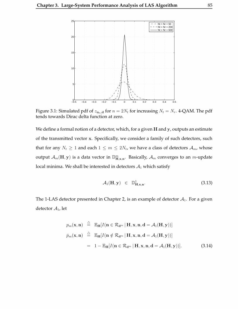
Chapter 3. Large-System Performance Analysis of LAS Algorithm 85
−0.5 −0.4 −0.3 −0.2 −0.1 0 0.1 0.2 0.3 0.4 0.50
5
10
15
20
25
Nt = Nr = 50Nt = Nr = 200Nt = Nr = 600
Figure 3.1: Simulated pdf of zun,d for n = 2Nt for increasing Nt = Nr. 4-QAM. The pdftends towards Dirac delta function at zero.
We define a formal notion of a detector, which, for a given H and y, outputs an estimate
of the transmitted vector x. Specifically, we consider a family of such detectors, such
that for any Nt ≥ 1 and each 1 ≤ m ≤ 2Nt, we have a class of detectors Am, whose
output Am(H,y) is a data vector in DmH,x,n. Basically, Am converges to an m-update
local minima. We shall be interested in detectors A1 which satisfy
A1(H,y) ∈ D1H,x,n. (3.13)
The 1-LAS detector presented in Chapter 2, is an example of detector A1. For a given
detector A1, let
pm(x,n)4= EH[I(n ∈ Rdm |H,x,n,d = A1(H,y))]
pm(x,n)4= EH[I(n /∈ Rdm |H,x,n,d = A1(H,y))]
= 1− EH[I(n ∈ Rdm |H,x,n,d = A1(H,y))]. (3.14)
Chapter 3. Large-System Performance Analysis of LAS Algorithm 86
For m = 2Nt, we simply drop the subscript and define
p(x,n)4= p2Nt(x,n), p(x,n)
4= p2Nt(x,n). (3.15)
Therefore, for a given (x,n), pm(x,n) denotes the probability that the output of the
detector A1 is an m-update local minima. We also define pr,s as
pr,s4= E(x,n)EH[I(n ∈ Rds |H,x,n,n ∈ Rdr ,d = A1(H,y))], (3.16)
i.e., the average probability that the output of the detector A1 is a s-update local min-
ima, conditioned on the fact that the output is a r-update local minima. From the
definition ofRdm , it is obvious that pr,s is 1 for s ≤ r.
We conjecture that a 1-update local minima is indeed a 2Nt-update local minima with
high probability, which is more formally stated as follows.
Conjecture 1. For any detector A1 with property (3.13) and any δ, 0 ≤ δ ≤ 1, there exists an
integer N(δ) such that for Nt > N(δ), and any (x,n), p(x,n) > 1− δ.
In Appendix C, we present arguments which makes us believe that this conjecture
could be indeed true. A more general form of the conjecture would be: Any detectorAm
converging to a m-update local minima, would have an output same as the ML vector with high
probability. It is easy to see from the analysis in Appendix C, that conjecture 1 stated for
A1 would only be true if the general conjecture were true for all m = 2, 3, · · · (2Nt − 1).
This therefore makes us believe that the general conjecture could also be true.
As shown in Appendix C, the validity of the conjecture rests on the validity of the fact
that for any 1 ≤ r < (2Nt − 1), if the detector output is a r-update local minima, then
it is indeed a r + 1-update local minima with high probability. This is equivalent to the
fact that the probabilities pr,r+1 are high (close to 1) for all 1 ≤ r < 2Nt − 1. Due to the
analytical difficulty involved in getting closed-form expressions for these probabilities,
we evaluate them through Monte-Carlo simulations.

Chapter 3. Large-System Performance Analysis of LAS Algorithm 87
1 2 3 4 5 6 7 8 90.91
0.92
0.93
0.94
0.95
0.96
0.97
0.98
0.99
1
log2(N
t)
Pro
babi
lity,
Pr,
r+1
p1,2
p2,3
p3,4
p 4,5
Nr = N
t, MMSE 1−LAS
4−QAM, SNR = 10 dB
Figure 3.2: Conditional probabilities pr,r+1 as a function of increasing Nt = Nr for the1-LAS detector with MMSE initial vector. 4-QAM and SNR = 10 dB.
In Fig. 3.2, we plot the probabilities pr,r+1 for the 1-LAS detector with r = 1, 2, 3, 4 and
MMSE initial vector (‘MMSE 1-LAS’ detector), for increasing Nt = Nr, 4-QAM, and
SNR = 10 dB. It is indeed observed that for a given r, pr,r+1 initially decreases with
increasing Nr = Nt, but eventually starts increasing for increasing Nt = Nr, and shows
the tendency to converge to 1 in the limit as Nt = Nr →∞. In Fig. 3.3, these probabili-
ties are shown for ‘Random 1-LAS’ detector (which is nothing but 1-LAS detector with
any random data vector as the initial vector). Observations similar to those made in
Fig. 3.2 for MMSE 1-LAS detector can be made for Random 1-LAS in Fig. 3.3; i.e., the
probabilities for 1-LAS with any starting vector tend to 1 for large Nt = Nr. Also, it can
be seen that for a given Nt = Nr the probability values are smaller with Random 1-LAS
compared to MMSE 1-LAS, indicating a faster convergence of MMSE 1-LAS compared
to Random 1-LAS. The observations in Figs. 3.2 and 3.3 strengthen the validity of the
conjecture 1, which is stated for any arbitrary detector converging to a 1-update local
minima, and any initial data vector. �
Finally, we present the following conjecture on the error probability of 1-LAS detector
and analyze it.

Chapter 3. Large-System Performance Analysis of LAS Algorithm 88
1 2 3 4 5 6 7 8 9
0.4
0.5
0.6
0.7
0.8
0.9
1
log2(N
t)
Pro
babi
lity,
Pr,
r+1
p1,2
p2,3
p3,4
p 4,5
Nr = N
t, Random 1−LAS
4−QAM, SNR = 10 dB
Figure 3.3: Conditional probabilities pr,r+1 as a function of increasing Nt = Nr for the1-LAS detector with Random initial vector. 4-QAM and SNR = 10 dB.
Conjecture 2. The data vector/bit error probability of the 1-LAS detector converges to that of
the ML detector as Nt, Nr →∞ with Nt = Nr.
Let dLAS be the final output symbol vector of the 1-LAS algorithm given x, H and n.
The algorithm satisfies property (3.13), and therefore conjecture 1 is applicable. With
A1(.) as the 1-LAS algorithm, p(x,n) can now be expressed as
p(x,n) = EH[I(n ∈ Rd |H,x,n,d = A1(H,y))]
= EH[I(n ∈ Rd |H,x,n,d = LAS(H,y) = dLAS)]
= EH[I(n ∈ RdLAS|H,x,n,d = LAS(H,y) = dLAS)]
= EH[I(dLAS = ML vector |H,x,n,d = LAS(H,y) = dLAS)]
= EH[I(dLAS = ML vector |H,x,n)] (3.17)
In the above derivation, we have used Lemma 3, which states that if n ∈ RdLAS, then
dLAS is indeed the ML vector for the given x, H and n.
Chapter 3. Large-System Performance Analysis of LAS Algorithm 89
Let us further define
P (dLAS = ML vector |x,n)4= EH[I(dLAS = ML vector |H,x,n)]
P (dLAS 6= ML vector |x,n)4= 1 − EH[I(dLAS = ML vector |H,x,n)]. (3.18)
Assuming conjecture 1 to be true, we can state that for any δ, 0 ≤ δ ≤ 1, there exists an
integer N(δ) such that for any Nt ≥ N(δ), and any (x,n),
P (dLAS = ML vector |x,n) > (1− δ). (3.19)
For any Nt ≥ N(δ) and a given (x,n), the conditional probability of symbol vector
error averaged over the distribution of H is given by
PLAS(error |x,n)4= EH[I(dLAS 6= x |H,x,n)]
= EH[I(dLAS 6= x,dLAS = ML vector |H,x,n)]
+ EH[I(dLAS 6= x,dLAS 6= ML vector |H,x,n)]
= P (dLAS 6= x,dLAS = ML vector |x,n)
+ P (dLAS 6= x,dLAS 6= ML vector |x,n)
= P (dLAS 6= x |dLAS = ML vector,x,n)P (dLAS = ML vector |x,n)
+ P (dLAS 6= x |dLAS 6= ML vector,x,n)P (dLAS 6= ML vector |x,n). (3.20)
From (3.19), we have P (dLAS 6= ML vector |x,n) ≤ δ. Also, P (dLAS 6= x |dLAS =
ML vector,x,n) can be bounded as follows. Firstly, using (3.19) we have
P (dLAS 6= x |dLAS = ML vector,x,n) =P (dLAS 6= x,dLAS = ML vector |x,n)
P (dLAS = ML vector |x,n)
<P (dLAS 6= x,dLAS = ML vector |x,n)
(1− δ). (3.21)

Chapter 3. Large-System Performance Analysis of LAS Algorithm 90
P (dLAS 6= x,dLAS = ML vector |x,n) can be expressed as
P (dLAS 6= x,dLAS = ML vector |x,n) = P (x 6= ML vector,dLAS = ML vector |x,n)
= P (x 6= ML vector |x,n)
−P (x 6= ML vector,dLAS 6= ML vector |x,n)
≤ P (x 6= ML vector |x,n). (3.22)
P (x 6= ML vector |x,n) is nothing but the probability of error of the ML detector (av-
eraged over the distribution of H) for a given x,n. Subsequently, we denote this by
PML(error |x,n). Using (3.21) and (3.22), we have
P (dLAS 6= x |dLAS = ML vector,x,n) <PML(error |x,n)
(1− δ). (3.23)
Using (3.23) in (3.20), PLAS(error |x,n) can be upper bounded as follows
PLAS(error |x,n) <PML(error |x,n)
(1− δ)+ δ P (dLAS 6= x |dLAS 6= ML vector,x,n)
≤ PML(error |x,n)
(1− δ)+ δ. (3.24)
Since the ML detector is the optimal detector w.r.t the symbol vector error probability,
we have
PML(error |x,n)
(1− δ)+ δ > PLAS(error |x,n) > PML(error |x,n). (3.25)
Let
M(x)4=
1
2
((x + 2)−
√x2 + 4
), x > 0. (3.26)
M(x) is a monotonically increasing function of x, which takes on positive values and
is bounded above by 1. Therefore, for a given 1 > δ > 0, there exists some x = ε such

Chapter 3. Large-System Performance Analysis of LAS Algorithm 91
that M(ε) = δ. Also M is an invertible function, and therefore it follows that
ε = δ(1 +
1
(1− δ)
). (3.27)
Using (3.25) and (3.27), the absolute difference between the error probability of the LAS
and the ML detector can be written as
|PLAS(error |x,n)− PML(error |x,n)| = (PLAS(error |x,n)− PML(error |x,n))
≤ PML(error |x,n)
(1− δ)+ δ − PML(error |x,n)
= δ(1 +
PML(error |x,n)
(1− δ)
)
≤ δ(1 +
1
(1− δ)
)= ε. (3.28)
We next define the averaged LAS and ML error probabilities as
PLAS(error)4= Ex,n[PLAS(error |x,n)] (3.29)
PML(error)4= Ex,n[PML(error |x,n)].
From (3.28), the bound on the absolute difference |PLAS(error |x,n)−PML(error |x,n)|
is independent of (x,n), and therefore averaging over (x,n) results in
|PLAS(error)− PML(error)| < ε. (3.30)
Hence, we have shown that for any arbitrary ε > 0, there exists a corresponding
positive real δ = M(ε) and an integer F (ε)4= N(M(ε)) = N(δ) such that, for all
Nt ≥ F (ε), |PLAS(error)−PML(error)| < ε. This proves that PLAS(error)→ PML(error)
as Nt → ∞. This analysis can be adapted to show that, apart from the symbol vector
error probability, the bit error probability of the LAS detector also converges to that of
the ML detector. The analysis for the bit error probability convergence is along similar
lines, except that instead of defining the error event as dLAS 6= x, we define error events

Chapter 3. Large-System Performance Analysis of LAS Algorithm 92
7 7.5 8 8.5 9 9.5 10 10.5 1110
−4
10−3
10−2
10−1
Average Received SNR (dB)
Bit
Err
or R
ate
Nt = Nr = 1
Nt = Nr = 10
Nt = Nr = 50
Nt = Nr = 100
Nt = Nr = 200
Nt = Nr = 600
SISO AWGN
BER improves withincreasing Nt = Nr
V−BLAST, 4−QAMMMSE initial vector
Figure 3.4: Simulated BER performance of the 1-LAS detector for V-BLAST MIMO asa function of average received SNR for increasing values of Nt = Nr. MMSE initialvector, 4-QAM.
for each bit. For example, for the pth bit, the error event is defined as dpLAS 6= xp. �
3.2 Simulation Results and Discussions
In Fig. 3.4, we show the simulated BER performance of the 1-LAS detector with MMSE
initial vector for V-BLAST MIMO as a function of SNR for increasing Nt = Nr. The
modulation alphabet is 4-QAM. Since an analytical expression for ML performance in
the large MIMO system limit is not available, and simulating the ML performance for
large dimensions involves prohibitively high complexity, we plot the SISO AWGN per-
formance as a lower bound for comparison. It can be seen that for increasing Nt = Nr,
the BER performance of the 1-LAS detector approaches the SISO AWGN performance
at high SNRs, which lends simulation support for conjecture 2.
In Figs. 3.5 and 3.6, we plot the simulated BER performance of the 1-LAS detector for
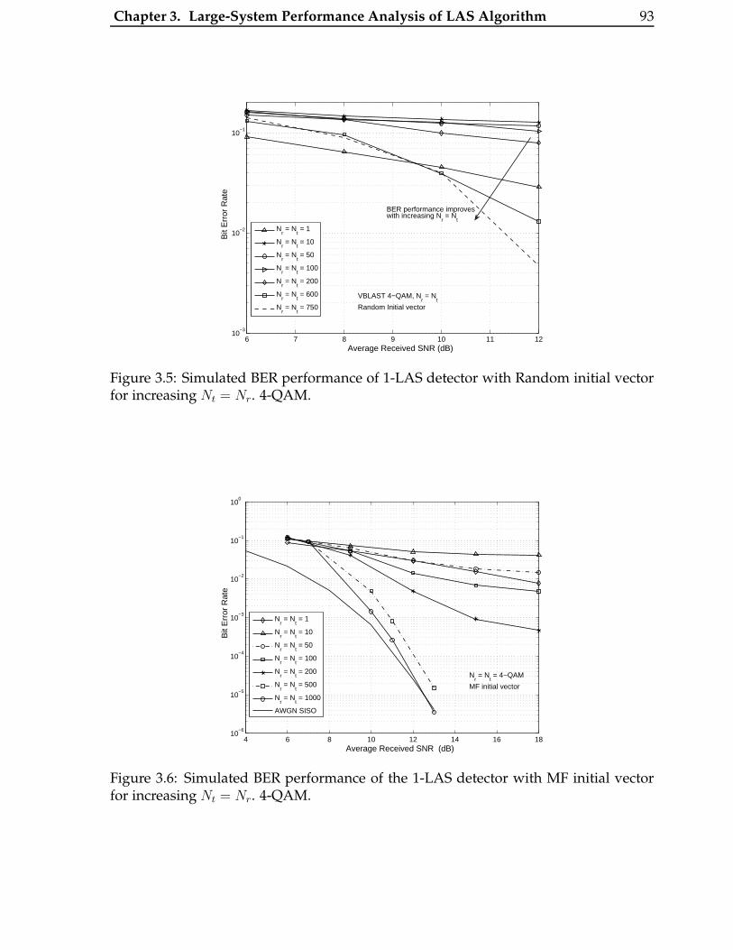
Chapter 3. Large-System Performance Analysis of LAS Algorithm 93
6 7 8 9 10 11 1210
−3
10−2
10−1
Average Received SNR (dB)
Bit
Err
or R
ate
Nr = N
t = 1
Nr = N
t = 10
Nr = N
t = 50
Nr = N
t = 100
Nr = N
t = 200
Nr = N
t = 600
Nr = N
t = 750
VBLAST 4−QAM, Nr = N
t
Random Initial vector
BER performance improveswith increasing N
r = N
t
Figure 3.5: Simulated BER performance of 1-LAS detector with Random initial vectorfor increasing Nt = Nr. 4-QAM.
4 6 8 10 12 14 16 1810
−6
10−5
10−4
10−3
10−2
10−1
100
Average Received SNR (dB)
Bit
Err
or R
ate
Nr = N
t = 1
Nr = N
t = 10
Nr = N
t = 50
Nr = N
t = 100
Nr = N
t = 200
Nr = N
t = 500
Nr = N
t = 1000
AWGN SISO
Nr = N
t = 4−QAM
MF initial vector
Figure 3.6: Simulated BER performance of the 1-LAS detector with MF initial vectorfor increasing Nt = Nr. 4-QAM.
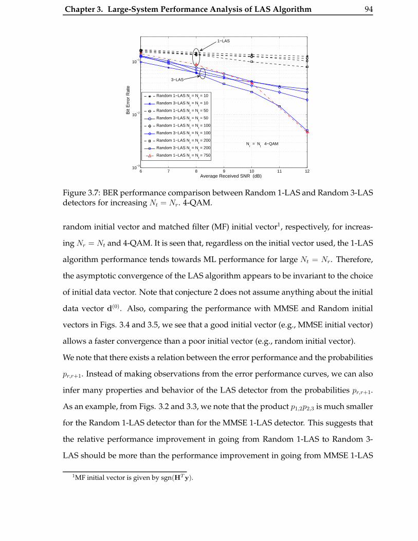
Chapter 3. Large-System Performance Analysis of LAS Algorithm 94
6 7 8 9 10 11 1210
−3
10−2
10−1
Average Received SNR (dB)
Bit
Err
or R
ate
Random 1−LAS Nr = N
t = 10
Random 3−LAS Nr = N
t = 10
Random 1−LAS Nr = N
t = 50
Random 3−LAS Nr = N
t = 50
Random 1−LAS Nr = N
t = 100
Random 3−LAS Nr = N
t = 100
Random 1−LAS Nr = N
t = 200
Random 3−LAS Nr = N
t = 200
Random 1−LAS Nr = N
t = 750
Nr = N
t 4−QAM
3−LAS
1−LAS
Figure 3.7: BER performance comparison between Random 1-LAS and Random 3-LASdetectors for increasing Nt = Nr. 4-QAM.
random initial vector and matched filter (MF) initial vector1, respectively, for increas-
ing Nr = Nt and 4-QAM. It is seen that, regardless on the initial vector used, the 1-LAS
algorithm performance tends towards ML performance for large Nt = Nr. Therefore,
the asymptotic convergence of the LAS algorithm appears to be invariant to the choice
of initial data vector. Note that conjecture 2 does not assume anything about the initial
data vector d(0). Also, comparing the performance with MMSE and Random initial
vectors in Figs. 3.4 and 3.5, we see that a good initial vector (e.g., MMSE initial vector)
allows a faster convergence than a poor initial vector (e.g., random initial vector).
We note that there exists a relation between the error performance and the probabilities
pr,r+1. Instead of making observations from the error performance curves, we can also
infer many properties and behavior of the LAS detector from the probabilities pr,r+1.
As an example, from Figs. 3.2 and 3.3, we note that the product p1,2p2,3 is much smaller
for the Random 1-LAS detector than for the MMSE 1-LAS detector. This suggests that
the relative performance improvement in going from Random 1-LAS to Random 3-
LAS should be more than the performance improvement in going from MMSE 1-LAS
1MF initial vector is given by sgn(HTy).
Chapter 3. Large-System Performance Analysis of LAS Algorithm 95
to MMSE 3-LAS. From the simulated error performance comparison between MMSE
1-LAS and MMSE 3-LAS presented in Chapter 2, and a similar comparison in Fig. 3.7,
we observe that, indeed, the relative performance improvement from 1-LAS to 3-LAS
is more for Random initial vector.

Chapter 4
Large-MIMO Detection Using
Probabilistic Data Association
In the previous two chapters, we dealt with LAS algorithm, which is a local neigh-
borhood search algorithm, and demonstrated its suitability for large-MIMO detection.
In this chapter, we present another low-complexity algorithm suited for large-MIMO
detection. The algorithm is based on probabilistic data association (PDA), which was
originally developed for target tracking, and is widely being employed in digital com-
munications [60]-[66]. PDA algorithm is a reduced complexity alternative to the a pos-
teriori probability (APP) decoder/detector/equalizer. In this chapter, we develop the
PDA algorithm for detection of MIMO signals, and demonstrate its suitability for large-
MIMO detection in terms of both performance and complexity [83].
4.1 System Model
We assume a MIMO channel with Nt transmit and Nr receive antennas. The NtNr
channel gains are modeled as i.i.d. CN (0,1). The channel gains are assumed to be
known at the receiver but not at the transmitter. We consider two types of MIMO
transmit architectures, namely, V-BLAST and STBC MIMO. As seen in Chapter 2, the
96
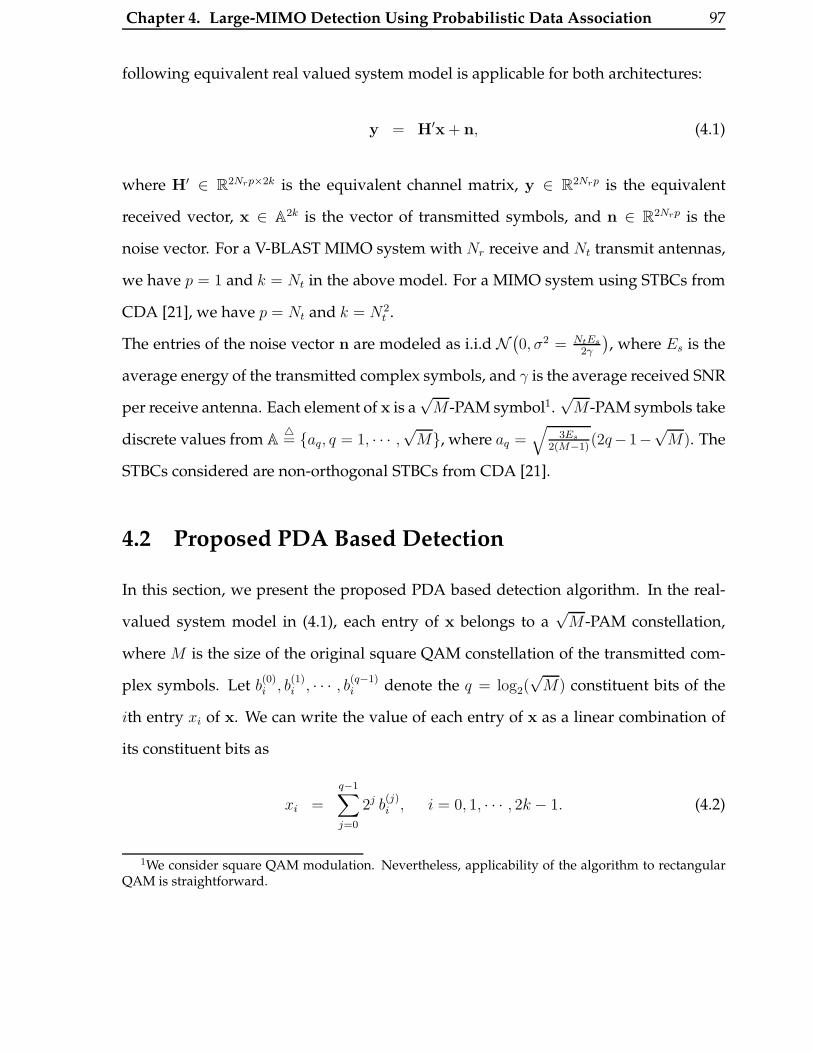
Chapter 4. Large-MIMO Detection Using Probabilistic Data Association 97
following equivalent real valued system model is applicable for both architectures:
y = H′x + n, (4.1)
where H′ ∈ R2Nrp×2k is the equivalent channel matrix, y ∈ R2Nrp is the equivalent
received vector, x ∈ A2k is the vector of transmitted symbols, and n ∈ R2Nrp is the
noise vector. For a V-BLAST MIMO system with Nr receive and Nt transmit antennas,
we have p = 1 and k = Nt in the above model. For a MIMO system using STBCs from
CDA [21], we have p = Nt and k = N2t .
The entries of the noise vector n are modeled as i.i.d N(0, σ2 = NtEs
2γ
), where Es is the
average energy of the transmitted complex symbols, and γ is the average received SNR
per receive antenna. Each element of x is a√
M -PAM symbol1.√
M -PAM symbols take
discrete values from A4= {aq, q = 1, · · · ,
√M}, where aq =
√3Es
2(M−1)(2q−1−
√M). The
STBCs considered are non-orthogonal STBCs from CDA [21].
4.2 Proposed PDA Based Detection
In this section, we present the proposed PDA based detection algorithm. In the real-
valued system model in (4.1), each entry of x belongs to a√
M -PAM constellation,
where M is the size of the original square QAM constellation of the transmitted com-
plex symbols. Let b(0)i , b
(1)i , · · · , b(q−1)
i denote the q = log2(√
M) constituent bits of the
ith entry xi of x. We can write the value of each entry of x as a linear combination of
its constituent bits as
xi =
q−1∑
j=0
2j b(j)i , i = 0, 1, · · · , 2k − 1. (4.2)
1We consider square QAM modulation. Nevertheless, applicability of the algorithm to rectangularQAM is straightforward.

Chapter 4. Large-MIMO Detection Using Probabilistic Data Association 98
Let b ∈ {+1,−1}2qk, defined as
b4=
[b(0)0 · · · b(q−1)
0 b(0)1 · · · b(q−1)
1 · · · b(0)2k−1 · · · b
(q−1)2k−1
]T, (4.3)
denote the transmitted bit vector. Defining c4= [20 21 · · · 2q−1], we can write x as
x = (I2k ⊗ c)b, (4.4)
using which we can rewrite (4.1) as
y = H′(I2k ⊗ c)︸ ︷︷ ︸4= H
b + n, (4.5)
where H ∈ R2Nrp×2qk is the effective channel matrix. The MAP estimate of bit b
(j)i is
b(j)i =
arg max
a ∈ {±1} p(b(j)i = a |y,H
), (4.6)
whose computational complexity is exponential in k. Our goal is to obtain b, an esti-
mate of b, at low complexities. For this, we iteratively update the statistics of each bit
of b, as described in the following subsection, for a certain number of iterations, and
hard decisions are made on the final statistics to get b.
4.2.1 Iterative Procedure
The algorithm is iterative in nature, where 2qk statistic updates, one for each of the
constituent bits, are performed in each iteration. We start the algorithm by initializing
the a priori probabilities as P (b(j)i = +1) = P (b
(j)i = −1) = 0.5, ∀ i = 0, · · · , 2k − 1 and
j = 0, · · · , q−1. In an iteration, the statistics of the bits are updated sequentially, i.e., the
ordered sequence of updates in an iteration is{b(0)0 , · · · , b(q−1)
0 , · · · · · · , b(0)2k−1, · · · b
(q−1)2k−1
}.
The steps involved in each iteration of the algorithm are derived as follows.
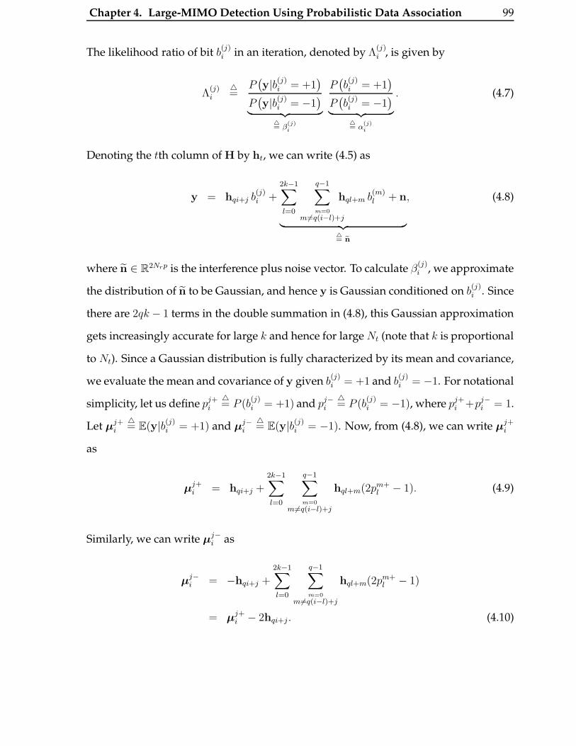
Chapter 4. Large-MIMO Detection Using Probabilistic Data Association 99
The likelihood ratio of bit b(j)i in an iteration, denoted by Λ
(j)i , is given by
Λ(j)i
4=
P(y|b(j)
i = +1)
P(y|b(j)
i = −1)
︸ ︷︷ ︸4= β
(j)i
P(b(j)i = +1
)
P(b(j)i = −1
)︸ ︷︷ ︸
4= α
(j)i
. (4.7)
Denoting the tth column of H by ht, we can write (4.5) as
y = hqi+j b(j)i +
2k−1∑
l=0
q−1∑
m=0
m6=q(i−l)+j
hql+m b(m)l + n
︸ ︷︷ ︸4= n
, (4.8)
where n ∈ R2Nrp is the interference plus noise vector. To calculate β(j)i , we approximate
the distribution of n to be Gaussian, and hence y is Gaussian conditioned on b(j)i . Since
there are 2qk − 1 terms in the double summation in (4.8), this Gaussian approximation
gets increasingly accurate for large k and hence for large Nt (note that k is proportional
to Nt). Since a Gaussian distribution is fully characterized by its mean and covariance,
we evaluate the mean and covariance of y given b(j)i = +1 and b
(j)i = −1. For notational
simplicity, let us define pj+i
4= P (b
(j)i = +1) and pj−
i
4= P (b
(j)i = −1), where pj+
i +pj−i = 1.
Let µj+i
4= E(y|b(j)
i = +1) and µj−i
4= E(y|b(j)
i = −1). Now, from (4.8), we can write µj+i
as
µj+i = hqi+j +
2k−1∑
l=0
q−1∑
m=0
m6=q(i−l)+j
hql+m(2pm+l − 1). (4.9)
Similarly, we can write µj−i as
µj−i = −hqi+j +
2k−1∑
l=0
q−1∑
m=0
m6=q(i−l)+j
hql+m(2pm+l − 1)
= µj+i − 2hqi+j . (4.10)

Chapter 4. Large-MIMO Detection Using Probabilistic Data Association 100
Next, the 2Nrp× 2Nrp covariance matrix, Cji , of y given bj
i is
Cji = E
{[n +
2k−1∑
l=0
q−1∑
m=0
m6=q(i−l)+j
hql+m(b(m)l − 2pm+
l + 1)]
·[n +
2k−1∑
l=0
q−1∑
m=0
m6=q(i−l)+j
hql+m(b(m)l − 2pm+
l + 1)]T}
. (4.11)
Assuming independence among the constituent bits, we can simplify Cji in (4.11) as
Cji = σ2I2Nrp +
2k−1∑
l=0
q−1∑
m=0
m6=q(i−l)+j
hql+m hTql+m 4pm+
l (1− pm+l ). (4.12)
Using the above mean and covariance, we can write the distribution of y given b(j)i =
±1 as
P (y|b(j)i = ±1) =
e−(y−µj±i )T (Cj
i )−1(y−µj±
i )
(2π)Nrp|Cji |
12
. (4.13)
Using (4.13), βji can be written as
βji = e−((y−µj+
i )T (Cji )
−1(y−µj+i )−(y−µj−
i )T (Cji )
−1(y−µj−i )). (4.14)
Using α(j)i and β
(j)i , Λ
(j)i is computed using (4.7). Using the value of Λ
(j)i , and using
P (b(j)i = +1|y) + P (b
(j)i = −1|y) = 1, the statistics of b
(j)i is updated as
P (b(j)i = +1|y) =
Λ(j)i
1 + Λ(j)i
, P (b(j)i = −1|y) =
1
1 + Λ(j)i
. (4.15)
This completes one iteration of the algorithm; i.e., each iteration involves the compu-
tation of α(j)i and (4.9), (4.10), (4.12), (4.14), (4.7), and (4.15) for all i, j. The updated
values of P (b(j)i = +1|y) and P (b
(j)i = −1|y) in (4.15) for all i, j are fed back as a priori
probabilities to the next iteration. The algorithm terminates after a certain number of
such iterations. At the end of the last iteration, decision is made on the final statistics

Chapter 4. Large-MIMO Detection Using Probabilistic Data Association 101
to obtain the bit estimate b(j)i as +1 if Λ
(j)i ≥ 1, and −1 otherwise. In coded systems,
Λ(j)i ’s are fed as soft inputs to the decoder.
4.2.2 Complexity Reduction
The most computationally expensive operation in computing β(j)i is the evaluation of
the inverse of the covariance matrix, Cji , of size 2Nrp × 2Nrp which requires O(N3
r p3)
complexity, which can be reduced as follows. Define matrix D as
D4= σ2I2Nrp +
2k−1∑
l=0
q−1∑
m=0
hql+mhTql+m4pm+
l (1− pm+l ). (4.16)
At the start of the algorithm, with pj+i = pj−
i = 0.5, ∀i, j, D becomes σ2I2Nrp + HHT .
Computation of D−1: When the statistics of b(j)i is updated using (4.15), the D matrix in
(4.16) also changes. Inversion of this updated D would require O(N3r p3) complexity.
However, D−1 can be obtained from the previously available D−1 in O(N2r p2) com-
plexity as follows. Since the statistics of only b(j)i is updated, the new D is just a rank
one update of the old D. So, using the matrix inversion lemma, the new D−1 can be
obtained from the old D−1 as
D−1 ← D−1 − D−1hni+jhTni+jD
−1
hTni+jD
−1hni+j + 1η
, (4.17)
where η = 4pj+i
(1− pj+
i
)− 4pj+
i,old
(1− pj+
i,old
), and pj+
i and pj+i,old are the new
(i.e., after the
update in (4.15))
and old (before the update) values, respectively. Both the numerator
and denominator in the 2nd term on the RHS of (4.17) can be computed in O(N2r p2)
complexity. So, the computation of the new D−1 using the old D−1 can be done in
O(N2r p2) complexity.
Computation of (Cji )
−1: Using (4.16) and (4.12), we can write Cji in terms of D as
Cji = D− 4pj+
i (1− pj+i )hqi+j hT
qi+j. (4.18)

Chapter 4. Large-MIMO Detection Using Probabilistic Data Association 102
We can compute (Cji )
−1 from D−1 at reduced complexity using the matrix inversion
lemma, as
(Cji )
−1 = D−1 − D−1 hqi+j hTqi+j D−1
hTqi+j D−1 hqi+j − 1
4pj+i (1−pj+
i )
, (4.19)
which can be computed in O(N2r p2) complexity.
Computation of µj+i and µ
j−i : Computation of β
(j)i involves the computation of µ
j+i and
µj−i also. From (4.10), it is clear that µ
j−i can be computed from µ
j+i with a compu-
tational overhead of only O(Nrp). From (4.9), it is seen that computing µj+i would
require O(qNrpk) complexity. However, this complexity can be reduced as follows.
Define vector u as
u4=
2k−1∑
l=0
q−1∑
m=0
hql+m
(2pm+
l − 1). (4.20)
Using (4.9) and (4.20), we can write µj+i = u + 2
(1 − pj+
i
)hqi+j . u can be computed
iteratively at O(Nrp) complexity as follows. When the statistics of b(j)i is updated, we
can obtain the new u from the old u as u ← u+2(pj+
i −pj+i,old
)hni+j , whose complexity
is O(Nrp). So, the computation of µj+i and µ
j−i needs O(Nrp) complexity. The full
listing of the proposed algorithm is presented in Table-4.1.
Overall Complexity: We need to compute HHT at the start of the algorithm. This re-
quires O(qkN2r p2) complexity. So the computation of the initial D−1 requires O(qkN2
r p2)+
O(N3r p3). Based on the complexity reduction in Section 4.2.2, the complexity in updat-
ing the statistics of one constituent bit is O(N2r p2). So, the complexity for the update of
all the 2qk constituent bits in an iteration is O(qkN2r p2). Since the number of iterations
is fixed, the overall complexity of the algorithm is O(qkN2r p2)+O(N3
r p3). Note that, for
a Nt = Nr V-BLAST MIMO system, since p = 1, the per bit complexity is O(N2t ), which
is the same as that of the LAS algorithm. However, in case of STBC, since p = Nt, PDA
has a per bit complexity of O(N4t ), which is an order higher than that of LAS.
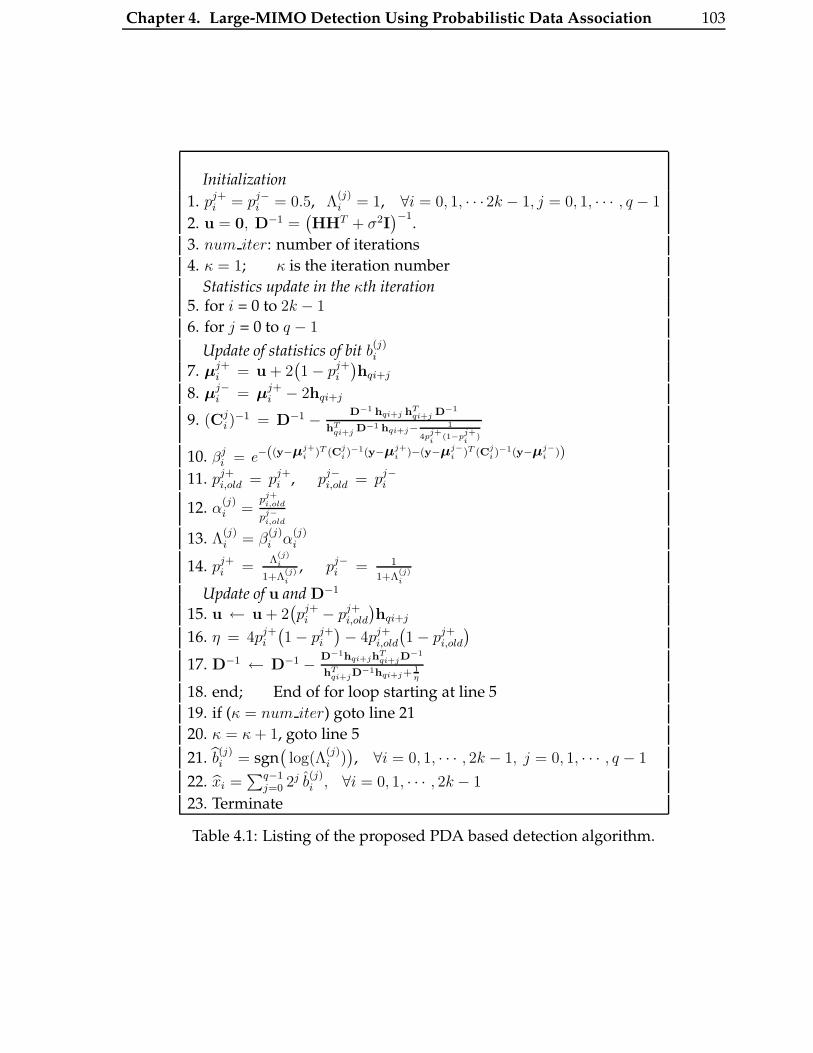
Chapter 4. Large-MIMO Detection Using Probabilistic Data Association 103
Initialization
1. pj+i = pj−
i = 0.5, Λ(j)i = 1, ∀i = 0, 1, · · ·2k − 1, j = 0, 1, · · · , q − 1
2. u = 0, D−1 =(HHT + σ2I
)−1.
3. num iter: number of iterations
4. κ = 1; κ is the iteration number
Statistics update in the κth iteration5. for i = 0 to 2k − 1
6. for j = 0 to q − 1
Update of statistics of bit b(j)i
7. µj+i = u + 2
(1− pj+
i
)hqi+j
8. µj−i = µ
j+i − 2hqi+j
9. (Cji )
−1 = D−1 − D−1 hqi+j hTqi+j D−1
hTqi+j D−1 hqi+j− 1
4pj+i
(1−pj+i
)
10. βji = e−((y−µ
j+i )T (Cj
i )−1(y−µ
j+i )−(y−µ
j−i )T (Cj
i )−1(y−µ
j−i ))
11. pj+i,old = pj+
i , pj−i,old = pj−
i
12. α(j)i =
pj+i,old
pj−i,old
13. Λ(j)i = β
(j)i α
(j)i
14. pj+i =
Λ(j)i
1+Λ(j)i
, pj−i = 1
1+Λ(j)i
Update of u and D−1
15. u ← u + 2(pj+
i − pj+i,old
)hqi+j
16. η = 4pj+i
(1− pj+
i
)− 4pj+
i,old
(1− pj+
i,old
)
17. D−1 ← D−1 − D−1hqi+jhTqi+jD
−1
hTqi+jD
−1hqi+j+1η
18. end; End of for loop starting at line 5
19. if (κ = num iter) goto line 21
20. κ = κ + 1, goto line 5
21. b(j)i = sgn
(log(Λ
(j)i )), ∀i = 0, 1, · · · , 2k − 1, j = 0, 1, · · · , q − 1
22. xi =∑q−1
j=0 2j b(j)i , ∀i = 0, 1, · · · , 2k − 1
23. Terminate
Table 4.1: Listing of the proposed PDA based detection algorithm.

Chapter 4. Large-MIMO Detection Using Probabilistic Data Association 104
0 2 4 6 8 10 12 1410
−5
10−4
10−3
10−2
10−1
100
Average Received SNR (dB)
Bit
Err
or R
ate
m = 1m = 2m = 4m = 8SISO AWGN
V−BLAST MIMONt = Nr = 64, 4−QAM
Figure 4.1: BER performance of PDA based detection in a V-BLAST MIMO system withNt = Nr = 64 and 4-QAM for different number of PDA iterations (m = 1, 2, 4, 8).
4.3 Results and Discussions
In this section, we present the simulated BER performance of the proposed PDA based
algorithm for detection in large V-BLAST and non-orthogonal STBC MIMO systems.
4.3.1 BER Performance in Large V-BLAST MIMO
BER performance with increasing number of PDA iterations: In Fig. 4.1, we plot the varia-
tion of the BER performance in a Nr = Nt = 64 V-BLAST MIMO system with 4-QAM,
for increasing number of PDA iterations (m = 1, 2, 4, 8). Perfect CSIR is assumed at the
receiver. It is observed that, as expected, the error performance improves with increase
in the number of iterations. However, the performance improvement for more than 4
iterations is observed to be marginal.
Large-System Behavior of PDA Based Detection: In Fig. 4.2, we plot the BER performance
of the PDA detector in V-BLAST MIMO with increasing number of transmit and re-
ceive antennas (Nt = Nr = 8, 16, 32, 64, 96) with 4-QAM and m = 5 iterations. It is seen
that the error performance improves with increasing Nt = Nr. This shows that the

Chapter 4. Large-MIMO Detection Using Probabilistic Data Association 105
0 2 4 6 8 10 12 14 1610
−5
10−4
10−3
10−2
10−1
100
Average Received SNR (dB)
Bit
Err
or R
ate
Nt = Nr = 8Nt = Nr = 16Nt = Nr = 32Nt = Nr = 64Nt = Nr = 96SISO AWGN
V−BLAST MIMO, Nt = Nr4−QAM, m = 5
Performance improveswith increasing Nt = Nr
.
Figure 4.2: BER performance of PDA based detection of V-BLAST MIMO for Nt = Nr =8, 16, 32, 64, 96, 4-QAM, and m = 5 iterations.
PDA algorithm, like the LAS algorithm in Chapter 2, exhibits large-system behavior,
making it suited for large-MIMO detection.
4.3.2 BER Performance in Large STBC MIMO
In this subsection, we present the simulated BER performance results for non-orthogonal
STBC MIMO systems with PDA detection. The MIMO channel is assumed to be quasi
static (i.e., fade remains constant for the duration of one STBC block, and i.i.d from
one STBC block to another). The STBCs used are ILL-only non-orthogonal STBCs from
CDA [21].
PDA versus LAS performance with 4-QAM: In Fig. 4.3, we plot the uncoded BER of
the PDA algorithm as a function of average received SNR per receive antenna, γ, in
decoding 4 × 4, 8 × 8, 16 × 16 ILL-only STBCs from CDA with Nt = Nr and 4-QAM.
Perfect CSIR and i.i.d fading are assumed. For the same settings, the performance of
the 1-LAS algorithm with MMSE initial vector is also plotted for comparison. From
Fig. 4.3, it is seen that i) as in V-BLAST MIMO, the PDA algorithm exhibits ‘large-
system behavior’ in STBC MIMO as well, i.e., BER improves with increased number of
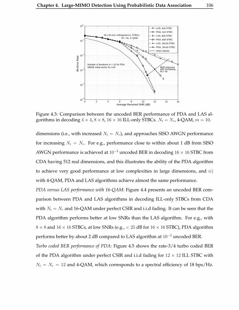
Chapter 4. Large-MIMO Detection Using Probabilistic Data Association 106
0 2 4 6 8 10 12 14 1610
−5
10−4
10−3
10−2
10−1
100
Average Received SNR (dB)
Bit
Err
or R
ate
LAS, 4x4 STBC
PDA, 4x4 STBC
LAS, 8x8 STBC
PDA, 8x8 STBC
LAS, 16x16 STBC
PDA, 16x16 STBC
SISO AWGN
BER improveswith increasingNt = Nr
Nt x Nt non−orthogonal ILL STBCsNt = Nr, 4−QAM
Number of iterations m = 10 for PDAMMSE initial vector for LAS
Figure 4.3: Comparison between the uncoded BER performance of PDA and LAS al-gorithms in decoding 4× 4, 8× 8, 16× 16 ILL-only STBCs. Nt = Nr, 4-QAM, m = 10.
dimensions (i.e., with increased Nt = Nr), and approaches SISO AWGN performance
for increasing Nt = Nr. For e.g., performance close to within about 1 dB from SISO
AWGN performance is achieved at 10−3 uncoded BER in decoding 16× 16 STBC from
CDA having 512 real dimensions, and this illustrates the ability of the PDA algorithm
to achieve very good performance at low complexities in large dimensions, and ii)
with 4-QAM, PDA and LAS algorithms achieve almost the same performance.
PDA versus LAS performance with 16-QAM: Figure 4.4 presents an uncoded BER com-
parison between PDA and LAS algorithms in decoding ILL-only STBCs from CDA
with Nt = Nr and 16-QAM under perfect CSIR and i.i.d fading. It can be seen that the
PDA algorithm performs better at low SNRs than the LAS algorithm. For e.g., with
8× 8 and 16× 16 STBCs, at low SNRs (e.g., < 25 dB for 16× 16 STBC), PDA algorithm
performs better by about 2 dB compared to LAS algorithm at 10−2 uncoded BER.
Turbo coded BER performance of PDA: Figure 4.5 shows the rate-3/4 turbo coded BER
of the PDA algorithm under perfect CSIR and i.i.d fading for 12 × 12 ILL STBC with
Nt = Nr = 12 and 4-QAM, which corresponds to a spectral efficiency of 18 bps/Hz.
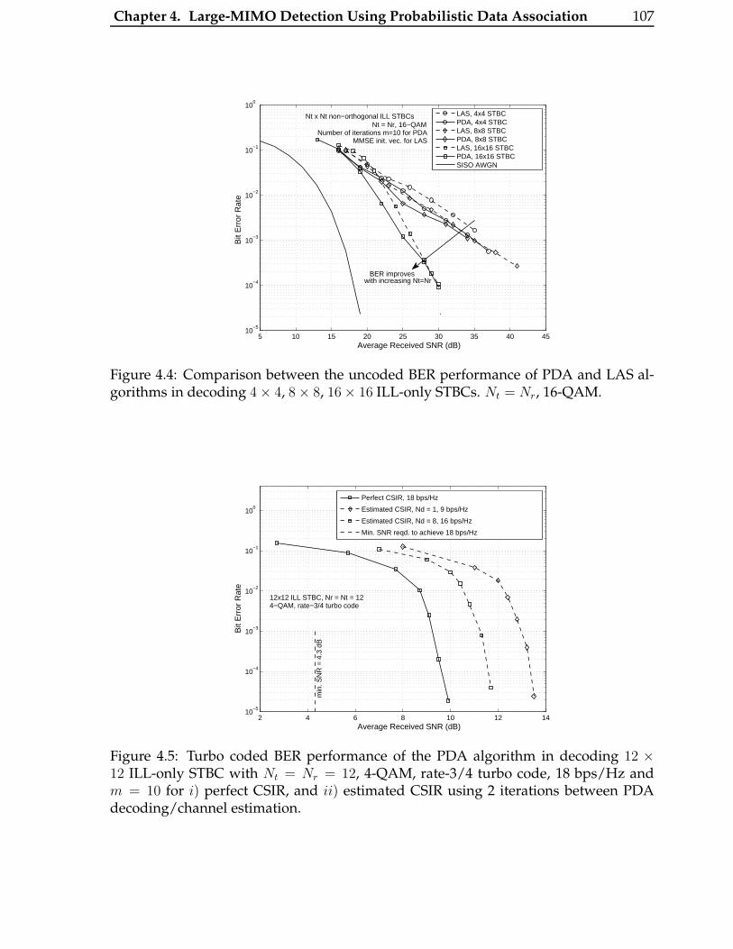
Chapter 4. Large-MIMO Detection Using Probabilistic Data Association 107
5 10 15 20 25 30 35 40 4510
−5
10−4
10−3
10−2
10−1
100
Average Received SNR (dB)
Bit
Err
or R
ate
LAS, 4x4 STBCPDA, 4x4 STBCLAS, 8x8 STBCPDA, 8x8 STBCLAS, 16x16 STBCPDA, 16x16 STBCSISO AWGN
Nt x Nt non−orthogonal ILL STBCsNt = Nr, 16−QAM
Number of iterations m=10 for PDAMMSE init. vec. for LAS
BER improves with increasing Nt=Nr
.
Figure 4.4: Comparison between the uncoded BER performance of PDA and LAS al-gorithms in decoding 4× 4, 8× 8, 16× 16 ILL-only STBCs. Nt = Nr, 16-QAM.
2 4 6 8 10 12 1410
−5
10−4
10−3
10−2
10−1
100
Average Received SNR (dB)
Bit
Err
or R
ate
Perfect CSIR, 18 bps/Hz
Estimated CSIR, Nd = 1, 9 bps/Hz
Estimated CSIR, Nd = 8, 16 bps/Hz
Min. SNR reqd. to achieve 18 bps/Hz
12x12 ILL STBC, Nr = Nt = 124−QAM, rate−3/4 turbo code
min
. SN
R =
4.3
dB
Figure 4.5: Turbo coded BER performance of the PDA algorithm in decoding 12 ×12 ILL-only STBC with Nt = Nr = 12, 4-QAM, rate-3/4 turbo code, 18 bps/Hz andm = 10 for i) perfect CSIR, and ii) estimated CSIR using 2 iterations between PDAdecoding/channel estimation.
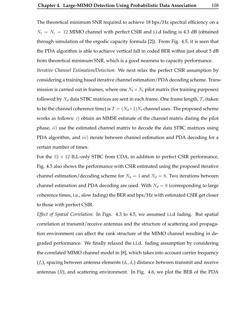
Chapter 4. Large-MIMO Detection Using Probabilistic Data Association 108
The theoretical minimum SNR required to achieve 18 bps/Hz spectral efficiency on a
Nt = Nr = 12 MIMO channel with perfect CSIR and i.i.d fading is 4.3 dB (obtained
through simulation of the ergodic capacity formula [2]). From Fig. 4.5, it is seen that
the PDA algorithm is able to achieve vertical fall in coded BER within just about 5 dB
from theoretical minimum SNR, which is a good nearness to capacity performance.
Iterative Channel Estimation/Detection: We next relax the perfect CSIR assumption by
considering a training based iterative channel estimation/PDA decoding scheme. Trans-
mission is carried out in frames, where one Nt×Nt pilot matrix (for training purposes)
followed by Nd data STBC matrices are sent in each frame. One frame length, T , (taken
to be the channel coherence time) is T = (Nd+1)Nt channel uses. The proposed scheme
works as follows: i) obtain an MMSE estimate of the channel matrix during the pilot
phase, ii) use the estimated channel matrix to decode the data STBC matrices using
PDA algorithm, and iii) iterate between channel estimation and PDA decoding for a
certain number of times.
For the 12 × 12 ILL-only STBC from CDA, in addition to perfect CSIR performance,
Fig. 4.5 also shows the performance with CSIR estimated using the proposed iterative
channel estimation/decoding scheme for Nd = 1 and Nd = 8. Two iterations between
channel estimation and PDA decoding are used. With Nd = 8 (corresponding to large
coherence times, i.e., slow fading) the BER and bps/Hz with estimated CSIR get closer
to those with perfect CSIR.
Effect of Spatial Correlation: In Figs. 4.3 to 4.5, we assumed i.i.d fading. But spatial
correlation at transmit/receive antennas and the structure of scattering and propaga-
tion environment can affect the rank structure of the MIMO channel resulting in de-
graded performance. We finally relaxed the i.i.d. fading assumption by considering
the correlated MIMO channel model in [8], which takes into account carrier frequency
(fc), spacing between antenna elements (dt, dr) distance between transmit and receive
antennas (R), and scattering environment. In Fig. 4.6, we plot the BER of the PDA
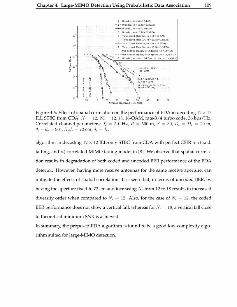
Chapter 4. Large-MIMO Detection Using Probabilistic Data Association 109
10 15 20 25 30 35 40 45 5010
−5
10−4
10−3
10−2
10−1
100
101
Nrd
r = 72 cm, d
t = d
r,
Dr = D
t = 20 m.
R = 500m, S= 30, f = 5 GHz. θ
t = θ
r = 90 deg.
Average Received SNR (dB)
Bit
Err
or R
ate
12x12 ILL STBC 16−QAM
min
. SN
R =
12.
6 dB
min
. SN
R =
9.4
dB
Uncoded, Nr = Nt = 12 (LAS)
Uncoded, Nr = 18, Nt = 12 (LAS)
Uncoded, Nr = Nt = 12 (PDA)
Uncoded, Nr = 18, Nt = 12 (PDA)
Turbo coded, Rate−3/4, Nr = Nt = 12 (LAS)
Turbo coded, Rate−3/4, Nr = 18, Nt = 12 (LAS)
Turbo coded, Rate−3/4, Nr = Nt = 12 (PDA)
Turbo coded, Rate−3/4, Nr = 18, Nt = 12 (PDA)
Min. SNR for capacity for 36 bps/Hz (Nr = Nt = 12)
Min. SNR for capacity for 36 bps/Hz (Nr = 18, Nt = 12)
Uncoded, Nr = Nt = 12 (PDA), i.i.d. (i.e., no correlation)
Figure 4.6: Effect of spatial correlation on the performance of PDA in decoding 12× 12ILL STBC from CDA. Nt = 12, Nr = 12, 18, 16-QAM, rate-3/4 turbo code, 36 bps/Hz.Correlated channel parameters: fc = 5 GHz, R = 500 m, S = 30, Dt = Dr = 20 m,θt = θr = 90◦, Nrdr = 72 cm, dt = dr.
algorithm in decoding 12 × 12 ILL-only STBC from CDA with perfect CSIR in i) i.i.d.
fading, and ii) correlated MIMO fading model in [8]. We observe that spatial correla-
tion results in degradation of both coded and uncoded BER performance of the PDA
detector. However, having more receive antennas for the same receive aperture, can
mitigate the effects of spatial correlation. It is seen that, in terms of uncoded BER, by
having the aperture fixed to 72 cm and increasing Nr from 12 to 18 results in increased
diversity order when compared to Nr = 12. Also, for the case of Nr = 12, the coded
BER performance does not show a vertical fall, whereas for Nr = 18, a vertical fall close
to theoretical minimum SNR is achieved.
In summary, the proposed PDA algorithm is found to be a good low-complexity algo-
rithm suited for large-MIMO detection.

Chapter 5
Large-MIMO Precoding Using X- and
Y-Codes
In this chapter, we consider precoding in large-MIMO systems, where CSI is perfectly
available both at the transmitter and the receiver. We propose precoding schemes
based on X- and Y-Codes to achieve high multiplexing and diversity gains at low
complexity [92]-[94]. The proposed precoding schemes are based upon the singular
value decomposition (SVD) of the channel matrix which transforms the MIMO chan-
nel into parallel subchannels. X- and Y-Codes are used to improve the diversity gain
by pairing the subchannels, prior to SVD precoding. In particular, the subchannels
with good diversity are paired with those having low diversity gains. Hence, a pair
of channels is jointly encoded using a 2 × 2 real matrix, which is fixed a priori and
does not change with each channel realization. For X-Codes these matrices are 2-
dimensional rotation matrices parameterized by a single angle, while for Y-Codes,
these matrices are 2-dimensional upper left triangular matrices. The complexity of
the maximum likelihood decoding for both X- and Y-Codes is low. Specifically, the
decoding complexity of Y-Codes is the same as that of a scalar channel. Moreover,
we propose X-, Y-Precoders with the same structure as X-, Y-Codes, but the encod-
ing matrices adapt to each channel realization. The optimal encoding matrices for X-,
110
Chapter 5. Large-MIMO Precoding Using X- and Y-Codes 111
Y-Codes/Precoders are derived analytically. It is observed that X-Codes/Precoders
perform better for well-conditioned channels, while Y-Codes/Precoders perform bet-
ter for ill-conditioned channels, when compared to other precoding schemes in the
literature.
This chapter is organized as follows. Section 5.1 introduces the system model and SVD
precoding. In Section 5.2, we present the pairing of subchannels as a general coding
strategy to achieve higher diversity order in fading channels. In Section 5.3, we pro-
pose the X-Codes and the X-Precoders. We show that ML decoding can be achieved
with Nr 2-D real sphere decoders (SD). We also analyze the error performance and
present the design of optimal X-Codes and X-Precoders. In Section 5.4, we propose
the Y-Codes and Y-Precoder. We show that they have very low decoding complex-
ity. We analyze the error performance and derive expressions for the optimal Y-Codes
and Y-Precoders. Section 5.5 shows the simulation results and comparisons with other
precoders. Section 5.6 discusses the complexity of the X-, Y-Codes/Precoders in com-
parison with other precoders.
5.1 System Model and SVD Precoding
We consider a Nt × Nr MIMO system (Nr ≤ Nt) with Nr receive and Nt transmit
antennas. CSI is assumed to be known perfectly at both transmitter and receiver. Let
x = (x1, · · · , xNt)T be the vector of symbols transmitted by the Nt transmit antennas,
and let H = {hij}, i = 1, · · · , Nr, j = 1, · · · , Nt, be the Nr × Nt channel coefficient
matrix, where hij is the complex channel gain between the jth transmit antenna and
the ith receive antenna, and hij’s are modeled as i.i.d. and CN (0, 1). The Nr×1 received
vector is given by
y = Hx + n, (5.1)

Chapter 5. Large-MIMO Precoding Using X- and Y-Codes 112
where n is a spatially uncorrelated Gaussian noise vector such that E[nnH ] = N0INr .
Such a system has a maximum multiplexing gain of Nr.
Let the number of transmitted information symbols be Ns (Ns ≤ Nr). The information
bits are first mapped to the information symbol vector u = (u1, · · · , uNs)T ∈ CNs , which
is then mapped to the data symbol vector z = (z1, · · · , zNs)T ∈ CNs using a Ns × Ns
matrix G as
z = Gu + u0, (5.2)
where u0 ∈ CNs is a displacement vector used to reduce the average transmitted power.
Let T be the Nt × Ns precoding matrix which is applied to the data symbol vector to
yield the transmitted vector
x = Tz. (5.3)
In general, T, G, and u0 are derived from the knowledge of H at the transmitter and
they are crucial to the system performance and complexity. The transmission power
constraint is given by
E[‖x‖2] = PT , (5.4)
where PT total transmit power, and we define the SNR as γ4= PT
N0.
The proposed X- and Y-Codes are based on the SVD precoding technique, which is
based on the singular value decomposition of the channel matrix H = UΛV, where
U ∈ CNr×Nr , Λ ∈ CNr×Nr , V ∈ CNr×Nt , UUH = VVH = INr , and Λ = diag(λ1, · · · , λNr),
with λ1 ≥ λ2 · · · ≥ λNr ≥ 0. Let V ∈ CNs×Nt be the submatrix with the first Ns rows of

Chapter 5. Large-MIMO Precoding Using X- and Y-Codes 113
V. The SVD precoder uses
T = VH
G = INs
u0 = 0, (5.5)
and the receiver gets
y = HTu + n. (5.6)
Let U ∈ CNr×Ns be the submatrix with the first Ns columns of U. The receiver then
computes
r = UHy = Λu + w, (5.7)
where w ∈ CNs is still an uncorrelated Gaussian noise vector with E[wwH ] = N0INs ,
Λ4= diag(λ1, · · · , λNs), and r = (r1, · · · , rNs)
T . SVD precoding therefore transforms the
channel into Ns parallel channels
ri = λiui + wi, i = 1, · · · , Ns, (5.8)
with non-negative fading coefficients λi. The overall error performance is dominated
by the minimum singular value λNs . When Ns = Nr = Nt, the resulting diversity order
is only 1.
5.2 Pairing Good and Bad Subchannels
Without loss of generality, we consider only the full-rate SVD precoding scheme with
even Nr and Ns = Nr. The matrix G ∈ CNr×Nr is now used to pair (jointly encode)

Chapter 5. Large-MIMO Precoding Using X- and Y-Codes 114
different subchannels in order to improve the diversity order of the system. The pre-
coding matrix T ∈ CNt×Nr and the transmitted vector x are given by
T = VH , x = VH(Gu + u0). (5.9)
Let the list of subchannel pairings be {(ik, jk) ∈ [1, Nr]× [1, Nr], k ∈ [1, Nr/2] | ik < jk}.
An example of a list of pairings with Nr = 6 is {(1, 6), (2, 5), (3, 4)}. A subchannel can
only be paired with some other channel exactly once. So {(1, 3), (1, 4), (2, 6)} is not
a valid pairing. On the k-th pair, consisting of subchannels ik and jk, the information
symbols uik and ujkare jointly coded using a 2×2 matrix Ak. In order to reduce the ML
decoding complexity, we restrict the entries of Ak to be real valued. Each Ak4= {ak,i,j},
i, j ∈ [1, 2], is a submatrix of the code matrix G as shown below:
gik,ik = ak,1,1 gik,jk= ak,1,2
gjk,ik = ak,2,1 gjk,jk= ak,2,2
(5.10)
where gi,j is the entry of G in the ith row and jth column.
We shall see later, that an optimal pairing in terms of achieving the best diversity order
is one in which the kth subchannel is paired with the (Nr − k + 1)th subchannel. For
e.g., with Nr = 6, the X-Code structure is given by
G =
a1,1,1 a1,1,2
a2,1,1 a2,1,2
a3,1,1 a3,1,2
a3,2,1 a3,2,2
a2,2,1 a2,2,2
a1,2,1 a1,2,2
, (5.11)
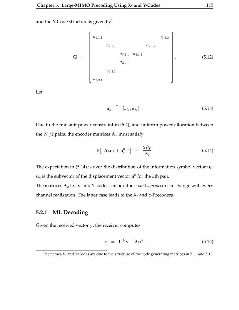
Chapter 5. Large-MIMO Precoding Using X- and Y-Codes 115
and the Y-Code structure is given by1
G =
a1,1,1 a1,1,2
a2,1,1 a2,1,2
a3,1,1 a3,1,2
a3,2,1
a2,2,1
a1,2,1
. (5.12)
Let
uk4= [uik , ujk
]T . (5.13)
Due to the transmit power constraint in (5.4), and uniform power allocation between
the Nr/2 pairs, the encoder matrices Ak must satisfy
E[‖Akuk + u0
k‖2]
=2PT
Nr
. (5.14)
The expectation in (5.14) is over the distribution of the information symbol vector uk.
u0k is the subvector of the displacement vector u0 for the kth pair.
The matrices Ak for X- and Y- codes can be either fixed a priori or can change with every
channel realization. The latter case leads to the X- and Y-Precoders.
5.2.1 ML Decoding
Given the received vector y, the receiver computes
r = UHy −Λu0. (5.15)
1The names X- and Y-Codes are due to the structure of the code generating matrices in 5.11 and 5.12.

Chapter 5. Large-MIMO Precoding Using X- and Y-Codes 116
Using (5.1) and (5.9), we can rewrite (5.15) as
r = ΛGu + w = Mu + w, (5.16)
where M4= ΛG is the equivalent channel gain matrix and w
4= UHn is a noise vector
with the same statistics as n. Further, we let
rk4= [rik , rjk
]T
wk4= [wik , wjk
]T .
Let Mk ∈ R2×2 denote the 2 × 2 submatrix of M consisting of entries in the ik and jk
rows and columns. Then (5.16) can be equivalently written as
rk = Mkuk + wk, k = 1, · · · , Nr
2. (5.17)
<(uk) ∈ Sk, where Sk is a finite signal set in the 2-dimensional real space. Assuming
that the same set is used for the imaginary component, the spectral efficiency, η, is
given by
η = 2
Nr2∑
k=1
log2(|Sk|). (5.18)
From (5.17), it is clear that the ML decoding (MLD) reduces to separate MLDs of the
k pairs, which can be further separated into independent ML decoding of the real and
imaginary components of uk. Then the MLD for the k-th pair is given by
<(uk) = arg min<(uk)∈Sk
‖<(rk)−Mk<(uk)‖2, (5.19)
and
=(uk) = arg min=(uk)∈Sk
‖=(rk)−Mk=(uk)‖2, (5.20)
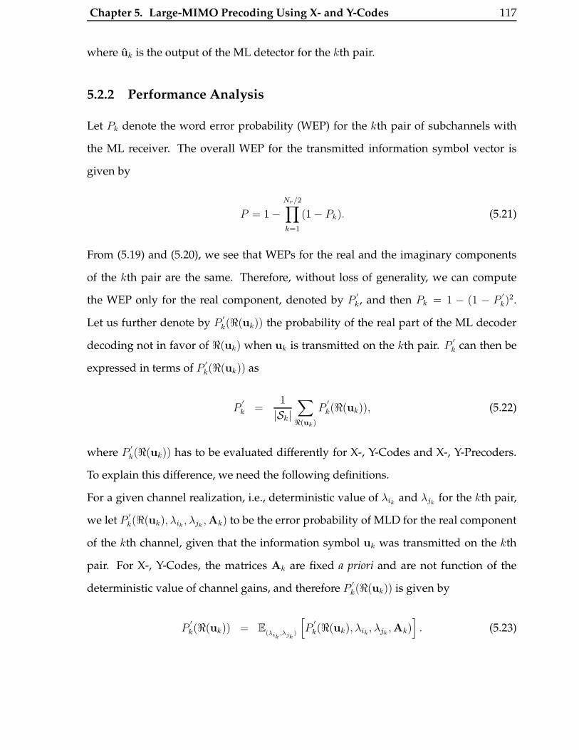
Chapter 5. Large-MIMO Precoding Using X- and Y-Codes 117
where uk is the output of the ML detector for the kth pair.
5.2.2 Performance Analysis
Let Pk denote the word error probability (WEP) for the kth pair of subchannels with
the ML receiver. The overall WEP for the transmitted information symbol vector is
given by
P = 1−Nr/2∏
k=1
(1− Pk). (5.21)
From (5.19) and (5.20), we see that WEPs for the real and the imaginary components
of the kth pair are the same. Therefore, without loss of generality, we can compute
the WEP only for the real component, denoted by P′
k, and then Pk = 1 − (1 − P′
k)2.
Let us further denote by P′
k(<(uk)) the probability of the real part of the ML decoder
decoding not in favor of <(uk) when uk is transmitted on the kth pair. P′
k can then be
expressed in terms of P′
k(<(uk)) as
P′
k =1
|Sk|∑
<(uk)
P′
k(<(uk)), (5.22)
where P′
k(<(uk)) has to be evaluated differently for X-, Y-Codes and X-, Y-Precoders.
To explain this difference, we need the following definitions.
For a given channel realization, i.e., deterministic value of λik and λjkfor the kth pair,
we let P′
k(<(uk), λik, λjk,Ak) to be the error probability of MLD for the real component
of the kth channel, given that the information symbol uk was transmitted on the kth
pair. For X-, Y-Codes, the matrices Ak are fixed a priori and are not function of the
deterministic value of channel gains, and therefore P′
k(<(uk)) is given by
P′
k(<(uk)) = E(λik
,λjk)
[P
′
k(<(uk), λik , λjk,Ak)
]. (5.23)
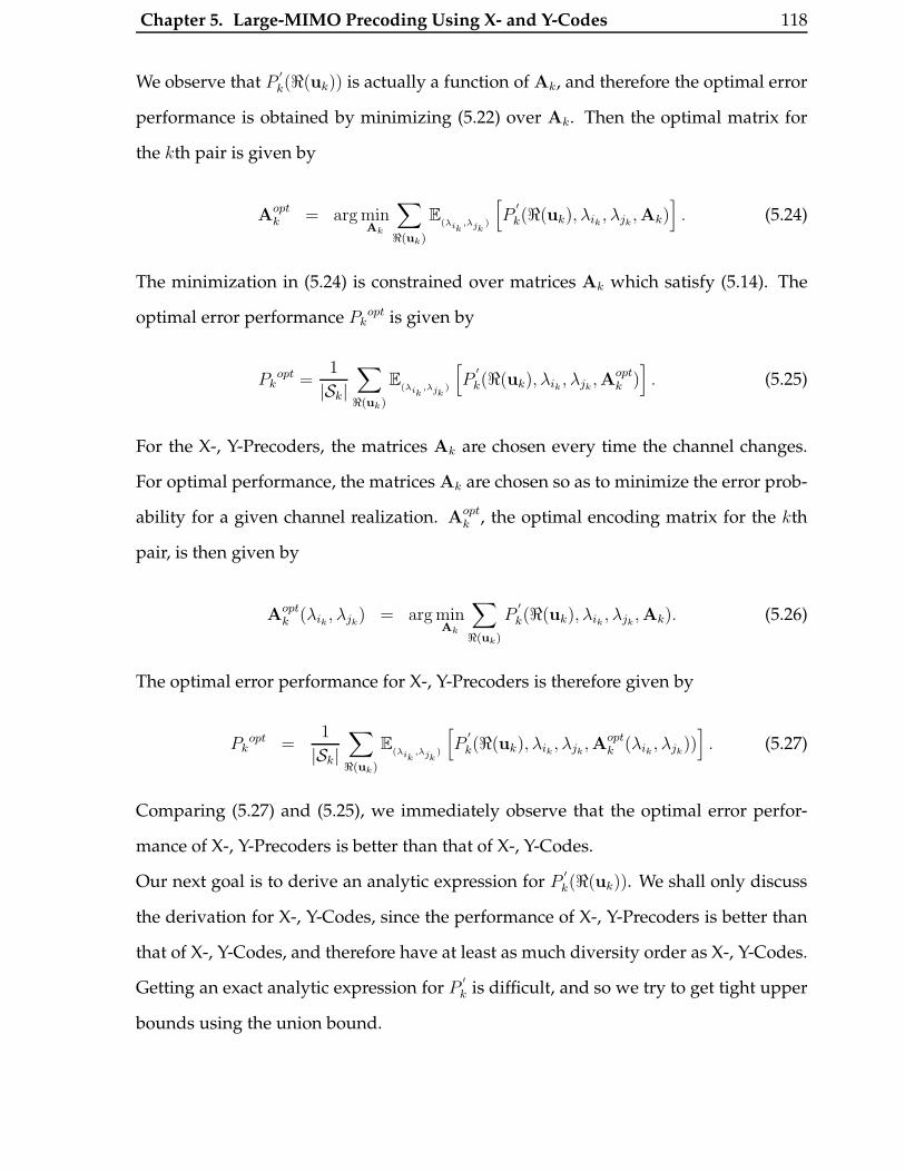
Chapter 5. Large-MIMO Precoding Using X- and Y-Codes 118
We observe that P′
k(<(uk)) is actually a function of Ak, and therefore the optimal error
performance is obtained by minimizing (5.22) over Ak. Then the optimal matrix for
the kth pair is given by
Aoptk = arg min
Ak
∑
<(uk)
E(λik
,λjk)
[P
′
k(<(uk), λik , λjk,Ak)
]. (5.24)
The minimization in (5.24) is constrained over matrices Ak which satisfy (5.14). The
optimal error performance Pkopt is given by
Pkopt =
1
|Sk|∑
<(uk)
E(λik
,λjk)
[P
′
k(<(uk), λik , λjk,Aopt
k )]. (5.25)
For the X-, Y-Precoders, the matrices Ak are chosen every time the channel changes.
For optimal performance, the matrices Ak are chosen so as to minimize the error prob-
ability for a given channel realization. Aoptk , the optimal encoding matrix for the kth
pair, is then given by
Aoptk (λik , λjk
) = arg minAk
∑
<(uk)
P′
k(<(uk), λik , λjk,Ak). (5.26)
The optimal error performance for X-, Y-Precoders is therefore given by
Pkopt =
1
|Sk|∑
<(uk)
E(λik
,λjk)
[P
′
k(<(uk), λik , λjk,Aopt
k (λik , λjk))]. (5.27)
Comparing (5.27) and (5.25), we immediately observe that the optimal error perfor-
mance of X-, Y-Precoders is better than that of X-, Y-Codes.
Our next goal is to derive an analytic expression for P′
k(<(uk)). We shall only discuss
the derivation for X-, Y-Codes, since the performance of X-, Y-Precoders is better than
that of X-, Y-Codes, and therefore have at least as much diversity order as X-, Y-Codes.
Getting an exact analytic expression for P′
k is difficult, and so we try to get tight upper
bounds using the union bound.
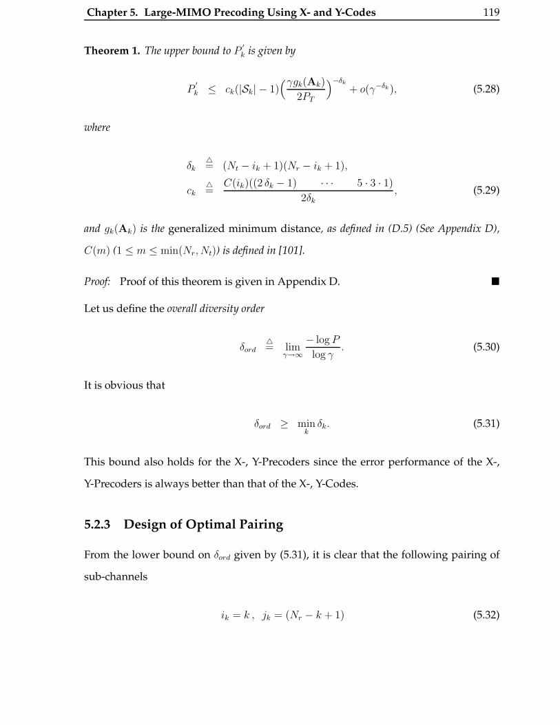
Chapter 5. Large-MIMO Precoding Using X- and Y-Codes 119
Theorem 1. The upper bound to P′
k is given by
P′
k ≤ ck(|Sk| − 1)(γgk(Ak)
2PT
)−δk
+ o(γ−δk), (5.28)
where
δk4= (Nt − ik + 1)(Nr − ik + 1),
ck4=
C(ik)((2 δk − 1) · · · 5 · 3 · 1)
2δk, (5.29)
and gk(Ak) is the generalized minimum distance, as defined in (D.5) (See Appendix D),
C(m) (1 ≤ m ≤ min(Nr, Nt)) is defined in [101].
Proof: Proof of this theorem is given in Appendix D. �
Let us define the overall diversity order
δord4= lim
γ→∞
− log P
log γ. (5.30)
It is obvious that
δord ≥ mink
δk. (5.31)
This bound also holds for the X-, Y-Precoders since the error performance of the X-,
Y-Precoders is always better than that of the X-, Y-Codes.
5.2.3 Design of Optimal Pairing
From the lower bound on δord given by (5.31), it is clear that the following pairing of
sub-channels
ik = k , jk = (Nr − k + 1) (5.32)

Chapter 5. Large-MIMO Precoding Using X- and Y-Codes 120
achieves the following best lower bound
δord ≥(Nr
2+ 1)(
Nt −Nr
2+ 1). (5.33)
Remark 1. Note that this corresponds to a cross-form generator matrix G, and is not the only
pairing for the best lower bound. Also, we note that the diversity order improves significantly,
when compared to the case of no pairing. It can be shown that if only Ns (Ns is even) out of the
Nr subchannels are used for transmission, the lower bound on the achievable diversity order is
(Nr − Ns
2+ 1)(Nt − Ns
2+ 1). �
Although it is hard to compute Aoptk , we can compute the best Ak, denoted by A?
k,
which minimizes the upper bound on Pk′ in (5.28). Then we have
A?k = arg max
Ak |E[‖Akuk+u0
k‖2]=
2PTNr
gk(Ak)
2PT. (5.34)
Using (5.28), (5.32) and (5.34), we obtain
P′
k ≤ ck(|Sk| − 1)(γgk(A
?k)
2PT
)−δ?k
+ o(γ−δ?k), (5.35)
where δ?k
4= (Nt − k + 1)(Nr − k + 1).
5.3 X-Codes and X-Precoder
5.3.1 X-Codes and X-Precoders: Encoding
For X-Codes, each symbol in u takes values from a regular M2-QAM constellation
which consists of the M-PAM constellation S 4= {τ(2i−(M−1)) |i = 0, 1, · · · , (M−1)}
used in quadrature on the real and the imaginary components of the channel. The
Chapter 5. Large-MIMO Precoding Using X- and Y-Codes 121
constant τ is
τ4=
√3Es
2(M2 − 1), (5.36)
and Es = PT
Nris the average symbol energy for each information symbol in the vector u.
Gray mapping is used to map the bits separately to the real and imaginary component
of the symbols in u. We fix u0 to be the zero vector. In order to avoid transmitter power
enhancement, we impose an orthogonality constraint on each Ak and parametrize it
with a single angle θk as
Ak =
cos(θk) sin(θk)
− sin(θk) cos(θk)
, k = 1, · · · , Nr/2. (5.37)
We notice that 1) both Ak and G are orthogonal, and 2) for X-Codes we fix the angles θk
a priori whereas for the X-Precoders we change the angles for each channel realization.
5.3.2 X-Codes and X-Precoders: ML Decoding
From (5.19) and (5.20) it is obvious that two 2-D real sphere decoders (SD) are needed
for each pair. Since there are Nr
2pairs, the total decoding complexity is Nr 2-D real SDs.
For X-Codes the matrices Mk in (5.19) and (5.20) are given by
Mk =
λik cos(θk) λik sin(θk)
−λjksin(θk) λjk
cos(θk)
. (5.38)
5.3.3 Optimal Design of X-Codes
In order to find the best angle θk for the kth pair, we attempt to maximize gk(Ak) under
the transmit power constraints. For X-Codes, let zk4= <(uk) − <(vk) be the difference
Chapter 5. Large-MIMO Precoding Using X- and Y-Codes 122
vector between any two information vectors, which can be written as
zk =
√6Es
(M2 − 1)(p, q)T , (p, q) ∈ SM , (5.39)
where
SM4=
{(p, q)
∣∣0 ≤ |p| ≤ (M − 1), 0 ≤ |q| ≤ (M − 1), (p, q) 6= (0, 0)}
. (5.40)
As defined in Appendix D, the generalized pairwise distance is
d2k(<(uk),<(vk),Ak) =
6PT
(p cos(θk) + q cos(θk)
)2
Nr(M2 − 1). (5.41)
Since Ak is parameterizable with a single angle θk, let
gk(θk, M)4= gk(Ak). (5.42)
Also, let
ϕp,q4= tan−1
(q
p
). (5.43)
Using (5.41) and (D.5), we have
gk(θk, M) =6PT min(p,q)∈SM
(p2 + q2) cos2(θk − ϕp,q)
Nr(M2 − 1). (5.44)
Using (5.34), the best θk, denoted by θ?k, is given by
θ?k = arg max
θk∈[0, π4]
min(p,q)∈SM
(p2 + q2) cos2(θk − ϕp,q). (5.45)

Chapter 5. Large-MIMO Precoding Using X- and Y-Codes 123
0 5 10 15 20 2510
−6
10−5
10−4
10−3
10−2
10−1
100
γ (dB)
Wor
d E
rror
Pro
babi
lity
Monte Carlo SimulationAnalytic upper bound
Nr = N
t = 2
X−Codes, θ1 = 27.8 deg, 4−QAM
Figure 5.1: Union bound for the word error probability. Nt = Nr = 2 and M = 2(4-QAM).
Following (5.35), the best achievable upper bound for P′
k is
P′
k ≤ (M2 − 1)ck
(3γgk(θ?k, M)
Nr(M2 − 1)
)−δ?k
+ o(γ−δ?k). (5.46)
Remark 2. It is easily shown by the symmetry of the set SM that it suffices to consider θk ∈
[0, π4] for the maximization in (5.45). The min-max optimization problem does not have explicit
analytical solutions except for small values of M , for example M = 2. But since the encoder
matrices are fixed a priori, these computations can be performed off-line. �
For small MIMO systems (e.g., for 2 × 2 MIMO), it is possible to get a tighter up-
per bound by evaluating the expectation in (D.3) (See Appendix D). P′
1 is then upper
bounded as
P′
1 ≤∑
(p,q)∈SM
(70/81)(M2 − 1)4γ−4
M2(p cos(θ1) + q sin(θ1))6(p2 + q2)+ o(γ−4), (5.47)
where θ1 is the angle used for the only pair. For larger MIMO systems, it is prefer-
able to use the inequality in (D.4) (See Appendix D), since evaluating the expectation
containing two singular values is tedious. In Fig. 5.1, we compare the WEP of a 2 × 2
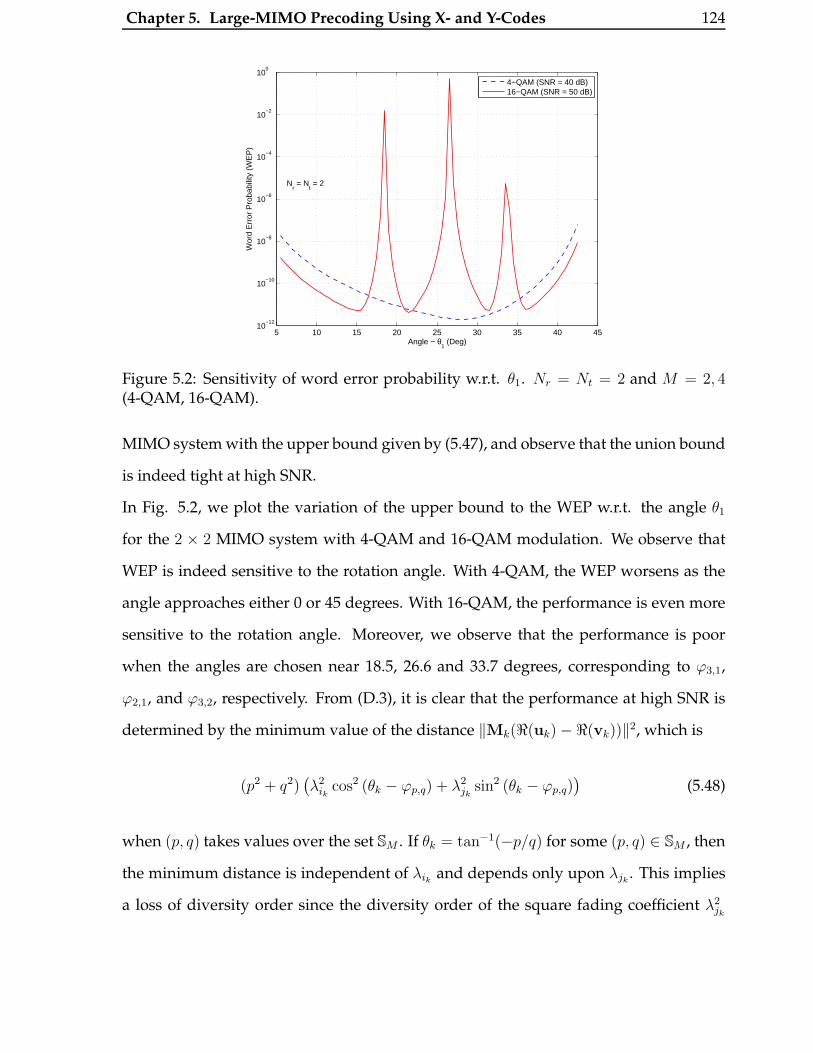
Chapter 5. Large-MIMO Precoding Using X- and Y-Codes 124
5 10 15 20 25 30 35 40 4510
−12
10−10
10−8
10−6
10−4
10−2
100
Angle − θ1 (Deg)
Wor
d E
rror
Pro
babi
lity
(WE
P)
4−QAM (SNR = 40 dB)16−QAM (SNR = 50 dB)
Nr = N
t = 2
Figure 5.2: Sensitivity of word error probability w.r.t. θ1. Nr = Nt = 2 and M = 2, 4(4-QAM, 16-QAM).
MIMO system with the upper bound given by (5.47), and observe that the union bound
is indeed tight at high SNR.
In Fig. 5.2, we plot the variation of the upper bound to the WEP w.r.t. the angle θ1
for the 2 × 2 MIMO system with 4-QAM and 16-QAM modulation. We observe that
WEP is indeed sensitive to the rotation angle. With 4-QAM, the WEP worsens as the
angle approaches either 0 or 45 degrees. With 16-QAM, the performance is even more
sensitive to the rotation angle. Moreover, we observe that the performance is poor
when the angles are chosen near 18.5, 26.6 and 33.7 degrees, corresponding to ϕ3,1,
ϕ2,1, and ϕ3,2, respectively. From (D.3), it is clear that the performance at high SNR is
determined by the minimum value of the distance ‖Mk(<(uk)− <(vk))‖2, which is
(p2 + q2)(λ2
ikcos2 (θk − ϕp,q) + λ2
jksin2 (θk − ϕp,q)
)(5.48)
when (p, q) takes values over the set SM . If θk = tan−1(−p/q) for some (p, q) ∈ SM , then
the minimum distance is independent of λik and depends only upon λjk. This implies
a loss of diversity order since the diversity order of the square fading coefficient λ2jk
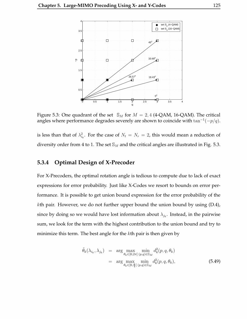
Chapter 5. Large-MIMO Precoding Using X- and Y-Codes 125
0 0.5 1 1.5 2 2.5 3 3.5 40
0.5
1
1.5
2
2.5
3
3.5
4
q
−p
set S2 (4−QAM)
set S4 (16−QAM)
0o
18.43o26.57o
45o
33.69o
Figure 5.3: One quadrant of the set SM for M = 2, 4 (4-QAM, 16-QAM). The criticalangles where performance degrades severely are shown to coincide with tan−1(−p/q).
is less than that of λ2ik
. For the case of Nt = Nr = 2, this would mean a reduction of
diversity order from 4 to 1. The set SM and the critical angles are illustrated in Fig. 5.3.
5.3.4 Optimal Design of X-Precoder
For X-Precoders, the optimal rotation angle is tedious to compute due to lack of exact
expressions for error probability. Just like X-Codes we resort to bounds on error per-
formance. It is possible to get union bound expression for the error probability of the
kth pair. However, we do not further upper bound the union bound by using (D.4),
since by doing so we would have lost information about λjk. Instead, in the pairwise
sum, we look for the term with the highest contribution to the union bound and try to
minimize this term. The best angle for the kth pair is then given by
θk(λik , λjk) = arg max
θk∈[0,2π]min
(p,q)∈SM
d2k(p, q, θk)
= arg maxθk∈[0, π
4]
min(p,q)∈SM
d2k(p, q, θk), (5.49)

Chapter 5. Large-MIMO Precoding Using X- and Y-Codes 126
where
d2k(p, q, θk)
4= (p2 + q2)(λ2
ikcos2(θk − ϕp,q) + λ2
jksin2(θk − ϕp,q)). (5.50)
Just like for X-Codes, it can be shown that for the maximization in (5.49), it suffices to
consider the range [0, π4] for θk. The optimization problem in (5.49) is difficult, but can
be solved exactly for small values of M . Also, the minimization over (p, q) ∈ SM need
not be over the full set containing |SM | = 4M(M − 1) elements. In fact, it can be shown
that the number of elements to be searched is at most (M2 − 3M + 6)/2. Therefore,
for M = 4 (16-QAM), we need not search over the full set of 48 elements, but rather it
suffices to search over only 5 elements.
Theorem 2. For M = 2 (4-QAM), the exact θk(λik , λjk) is given by
π/4, βk ≤√
3
tan−1[(β2k − 1)−
√((β2
k − 1)2 − β2k)], βk >
√3,
(5.51)
where
βk4=
λik
λjk
. (5.52)
βk is the ratio of subchannel gains, also known as the channel condition number.
Proof: Proof of this theorem is given in Appendix E. �
Further, let
d2k,min(λik , λjk
)4= max
θk∈[0, π4]
min(p,q)∈SM
d2k(p, q, θk). (5.53)
Using (5.53), the union bound to P′
k is given by
P′
k ≤ (M2 − 1)E
Q
√
d2k,min(λik , λjk
)
2N0
. (5.54)

Chapter 5. Large-MIMO Precoding Using X- and Y-Codes 127
The expectation in (5.54) is over the joint distribution of (λik , λjk) and is difficult to
compute analytically. We therefore use Monte-Carlo simulations to evaluate the exact
error probability.
5.4 Y-Codes and Y-Precoder
5.4.1 Motivation
It is observed that the error performance at high SNR is dependent on the minimum
value of the distance d2k(<(uk),<(vk),Ak) over all possible information vectors uk 6= vk.
Using the definition for d2k(<(uk),<(vk),Ak) (see Appendix D), we have
d2k(<(uk),<(vk),Ak) = ‖Mk(<(uk)− <(vk))‖2
= λ2ik
e2k,1 + λ2
jke2
k,2, (5.55)
where ek
4= Ak(<(uk)− <(vk)).
Let βk be the condition number of the equivalent channel for the kth pair (see Theorem
2). We have βk ≥ 1, since λik ≥ λjk. For the special case of βk = 1, d2
k(<(uk),<(vk),Ak)
is proportional to ‖ek‖2, which is the Euclidean distance between the code vectors. In
such a scenario, it is known that for large M choosing the code vectors as points of
the 2-dimensional hexagonal lattice would yield codes with good error performance.
However, the design of good codes becomes difficult for values of βk > 1. We im-
mediately notice that the effective euclidean distance in (5.55) gives more weight to
e2k,1 which is the difference of the vectors along the first component (since λik > λjk
).
Since the total transmit power is constrained, codes should be designed such that the
minimum separation of any two code vectors is more along the first component.
For X-Codes and X-Precoder, minimum separation was increased by rotating the QAM
constellation by an optimal angle. However, with this approach, apart from gaining
separation along the first component, we also achieve separation along the second

Chapter 5. Large-MIMO Precoding Using X- and Y-Codes 128
component. It is noted that the same diversity order can be achieved even if the min-
imum separation along the second component is small. Since the average transmit
power is constrained, optimal code design would try to choose code vectors such that
for the same transmit power, more separation is achieved along the first component
(without caring much about the separation achieved along the second component).
This observation along with the motivation of further reducing the decoding complex-
ity leads to the design of Y-Codes and Y-Precoder.
5.4.2 Y-Codes and Y-Precoders: Encoding
The matrices Ak have the structure
Ak =
ak 2ak
2bk 0
, (5.56)
where ak, bk ∈ R+. Let Sk be the set of pairs of integers defined by the Cartesian product
Sk4=
{[0, 1]×
[0, . . . ,
M
2− 1
]}. (5.57)
For e.g., with M = 4, the set Sk is given by
Sk ={[0, 0]T , [0, 1]T , [1, 0]T , [1, 1]T
}. (5.58)
We consider the 2-D codebook of cardinality M generated by applying Ak to the el-
ements of Sk and translating by u0k. The code vectors Yk(v), v = 1, · · · , M , are given
by
Yk(v) =
[ak
((v − 1)− M − 1
2
), bk(−1)v
]T
, (5.59)
The real and imaginary components of the displacement vector for the kth pair, u0k, are
Chapter 5. Large-MIMO Precoding Using X- and Y-Codes 129
given by
<(u0k) = =(u0
k) =
[−(M − 1)ak
2, −bk
]T
. (5.60)
Due to the transmit power constraint in (5.14), ak and bk must satisfy
b2k + a2
k
M2 − 1
12=
PT
Nr
. (5.61)
Information bits are Gray mapped to codebook indices in such a way that the Ham-
ming distance between bit vectors corresponding to close by (in terms of Euclidean
distance) code vectors is as small as possible. The only difference between Y-Codes
and Y-Precoders is that, for Y-Codes the parameters ak and bk are fixed a priori, whereas
for the Y-Precoders these are chosen every time the channel changes.
5.4.3 Y-Codes and Y-Precoders: ML Decoding
Using our codebook notation, the ML decoding rule in (5.19) and (5.20) can be equiva-
lently written as
v(I)k = arg min
v∈{0,··· ,(M−1)}‖<(rk)−ΛkYk(v)‖2, (5.62)
v(Q)k = arg min
v∈{0,··· ,(M−1)}‖=(rk)−ΛkYk(v)‖2, (5.63)
where v(I)k and v
(Q)k are ML estimates of the codeword indices transmitted on the real
and imaginary components for the kth pair.
We next discuss a low complexity algorithm for the optimization problem in (5.62).
The algorithm is the same for all pairs, and the same for both the real and imaginary
components of each pair. Therefore, we only discuss the algorithm for the real com-
ponent. We first partition the 2-D received signal space (R2) into(
M2
+ 1)
regions as
Chapter 5. Large-MIMO Precoding Using X- and Y-Codes 130
follows.
R0 :
{[x, y]T ∈ R
2| −∞ ≤(
x
λikak+
M − 1
2
)≤ 1
}, (5.64)
RM2
:
{[x, y]T ∈ R
2|(M − 1) ≤(
x
λikak+
M − 1
2
)≤ +∞
}, (5.65)
Ri :
{[x, y]T ∈ R
2|(2i− 1) ≤(
x
λikak
+M − 1
2
)≤ (2i + 1)
}, (5.66)
where i ∈ [1, M/2− 1]. In Fig. 5.4, we illustrate the 5 regions with M = 8 for the real
component of the kth pair.
We next discuss a low complexity ML decoding algorithm for Y-Codes. The first step
of the decoding algorithm is to find the region to which the received vector belongs.
Let
tk =
⌊<(rik)
2λikak+
M + 1
4
⌋. (5.67)
The received vector belongs to the region Rζk, where ζk is explicitly given by
ζk =
0 tk ≤ 0
M2
tk ≥ M2
tk otherwise.
(5.68)
For e.g., in Fig. 5.4, the received vectors p1, p2, and p3 belong to R0, R1, and R3,
respectively. It can be shown that once the received vector is decoded to the region Rζk,
the ML code vector is one among a reduced set of at most 3 code vectors. Therefore,
at most 3 Euclidean distances need to be computed to solve the ML detection problem
in (5.62), as compared to computing all the M Euclidean distances in case of a brute
force search. For e.g., in Fig. 5.4, for the received vector p3 ∈ R3, the ML code vector is
among Yk(6), Yk(7) or Yk(8).
However, once we know the region of the received vector, it is possible to directly find

Chapter 5. Large-MIMO Precoding Using X- and Y-Codes 131
−4 −3 −2 −1 0 1 2 3 4−3
−2
−1
0
1
2
3
 (rik
)/λik
ak
Â(r
j k)/λ j kb k
1
2
3
4
5
6
7
8
R0
R1
R2 R
3R
4
p1
p2
p3
Figure 5.4: Received signal space for the real component of the kth pair. M = 8 and sowe have 5 regions with vertical dashed lines demarcating the boundary between theregions. The scaled codebook vectors are represented by small filled circles along withtheir corresponding codebook index number. Dotted lines demarcate the boundarybetween the ML decision regions.
the ML code vector even without computing the 3 Euclidean distances. This involves
just checking a few linear relations between the 2 components of the received vector.
Therefore, the ML decoding complexity of Y-Codes is the same as that of a scalar chan-
nel. For e.g., in Fig. 5.4, the received vector p3 is to the right of the perpendicular
bisector between Yk(6) and Yk(8). p3 is also above the perpendicular bisector between
Yk(7) and Yk(8). From these two checks it can be easily concluded that the ML code
vector is Yk(8). Due to the structure of the codebook, the ML decision regions can be
very easily outlined. In Fig. 5.4, the dotted lines demarcate the boundary of the ML
decision regions. The hatched region illustrates the ML decision region of Yk(5).
5.4.4 Optimal Design of Y-Codes
Given the optimal pairing in (5.32), the next step towards designing optimal Y-Codes
is to find the optimal value of (ak, bk) which minimizes the average error probability.
For Y-Codes, once chosen, (ak, bk) are fixed and do not change with every channel

Chapter 5. Large-MIMO Precoding Using X- and Y-Codes 132
realization. Since the ML decision regions are known precisely, it is possible to calculate
the exact error probability. With our new codebook notation, we identify code vectors
by their index in the codebook, and the error probability is given by
P′
k =1
M
∑
v
P′
k(v), (5.69)
where P′
k(v) is the probability of error when the code vector Yk(v) is transmitted. P′
k(v)
is given by
P′
k(v) =
E[g1(ak, bk)], 3 ≤ v ≤ (M − 2)
E[g2(ak, bk)], v = 1, M
E[g1(ak, bk)− g3(ak, bk)], v = 2, (M − 1),
where the expectation is over the joint distribution of (λik , λjk). Let
Ψk(x)4=
√2(2akλikx− a2
kλ2ik− 4b2
kλ2jk
)
4bkλjk
√N0
, (5.70)
and
Φk(x)4= −
√2(2akλikx + a2
kλ2ik
+ 4b2kλ
2jk
)
4bkλjk
√N0
. (5.71)
The functions g1(ak, bk), g2(ak, bk) and g3(ak, bk) are given by
g1(ak, bk)4= 1−
∫ λikak
0
2e−x2
N0√πN0
Q (Ψk(x)) dx,
g2(ak, bk)4= 1−
∫ λikak
−∞
e−x2
N0√πN0
Q (Ψk(x)) dx,
g3(ak, bk)4=
∫ −λikak
−∞
e−x2
N0√πN0
Q (Φk(x)) dx. (5.72)
Chapter 5. Large-MIMO Precoding Using X- and Y-Codes 133
To compute the optimal (ak, bk), we have to minimize P′
k w.r.t. (ak, bk) subject to the
transmit power constraint in (5.61). However, it is difficult to get closed-form expres-
sions for the optimal (ak, bk) due to the intractability of the integrals in (5.72). This
difficulty is further compounded due to the evaluation of expectation over the joint
distribution of (λik , λjk). However, since (ak, bk) are fixed a priori, it is always possible
to approximately compute the optimal (ak, bk) off-line, using Monte-Carlo techniques.
5.4.5 Optimal Design of Y-Precoder
For the Y-Precoder, finding the optimal (ak, bk) for each channel realization is again
difficult due to the intractability of the integrals in (5.72). In the case of Y-Codes, these
could be computed off-line since (ak, bk) are fixed a priori. However, for Y-Precoders
these cannot be computed off-line, since the optimal (ak, bk) have to be computed every
time the channel changes. Therefore, we try to optimize (ak, bk) by minimizing the
union bound for P′
k. The union bound is given by
P′
k ≤ (M − 1)E
Q
√
d2k,min(ak, bk)
2N0
, (5.73)
where the expectation is over the joint distribution of (λik , λjk) and
d2k,min(ak, bk)
4= min
v 6=w
(λ2
ika2
k(v − w)2 + λ2jk
b2k((−1)v − (−1)w)2
), (5.74)
where v and w are distinct indices of the codebook.
The optimal choice of (ak, bk), denoted by (a?k, b
?k), which maximizes d2
k,min(ak, bk) for
the fixed channel gain of (λik , λjk), is given by the following theorem.
Theorem 3. The optimal value of (ak, bk) defined as
(a?k, b
?k)
4= arg max{
(ak ,bk)∈(R+)2|b2k+a2
kM2−1
12=
PTNr
} d2k,min(ak, bk), (5.75)
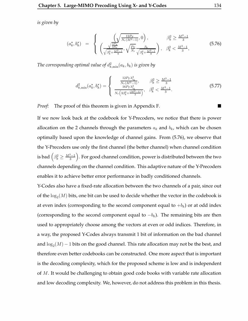
Chapter 5. Large-MIMO Precoding Using X- and Y-Codes 134
is given by
(a?k, b
?k) =
(√12PT
Nr(M2−1), 0)
, β2k ≥ M2−1
3( √4PT3Nr√
β2k+ M2−1
9
,√
PT
Nr
βk√β2
k+ M2−19
), β2
k < M2−13
,(5.76)
The corresponding optimal value of d2k,min(ak, bk) is given by
d2k,min(a
?k, b
?k) =
12PT λ2ik
Nr(M2−1), β2
k ≥ M2−13
16PT λ2ik
Nr
(3β2
k+(M2−1)
3
) , β2k < M2−1
3.
(5.77)
Proof: The proof of this theorem is given in Appendix F. �
If we now look back at the codebook for Y-Precoders, we notice that there is power
allocation on the 2 channels through the parameters ak and bk, which can be chosen
optimally based upon the knowledge of channel gains. From (5.76), we observe that
the Y-Precoders use only the first channel (the better channel) when channel condition
is bad(β2
k ≥ M2−13
). For good channel condition, power is distributed between the two
channels depending on the channel condition. This adaptive nature of the Y-Precoders
enables it to achieve better error performance in badly conditioned channels.
Y-Codes also have a fixed-rate allocation between the two channels of a pair, since out
of the log2(M) bits, one bit can be used to decide whether the vector in the codebook is
at even index (corresponding to the second component equal to +bk) or at odd index
(corresponding to the second component equal to −bk). The remaining bits are then
used to appropriately choose among the vectors at even or odd indices. Therefore, in
a way, the proposed Y-Codes always transmit 1 bit of information on the bad channel
and log2(M)− 1 bits on the good channel. This rate allocation may not be the best, and
therefore even better codebooks can be constructed. One more aspect that is important
is the decoding complexity, which for the proposed scheme is low and is independent
of M . It would be challenging to obtain good code books with variable rate allocation
and low decoding complexity. We, however, do not address this problem in this thesis.
Chapter 5. Large-MIMO Precoding Using X- and Y-Codes 135
5.5 Simulation Results
In this section, we compare the performance of X-, Y-Codes and X-, Y-Precoders with
other precoders. For all the simulations, we assume Nt = Nr. Pairing of subchan-
nels is given by (5.32). The optimal matrices Ak are chosen as discussed previously.
Comparisons are made with i) the E-dmin (equal dmin precoder proposed in [102]), ii)
the Arithmetic mean BER precoder (ARITH-MBER) proposed in [25], iii) the Equal En-
ergy linear precoder (EE) based upon optimizing the minimum eigenvalue for a given
transmit power constraint [26]), iv) the TH precoder based upon the idea of Tomlinson-
Harashima precoding applied in the MIMO context [27]), and v) the channel inversion
(CI) known as zero-forcing precoder [103].
5.5.1 Effect of Channel Condition on Error Performance
In Fig. 5.5, we plot the error performance of all precoding schemes for a 2 × 2 MIMO
system at γ = 26dB, as a function of the condition number β = λ1/λ2. We fix the
total channel gain λ12 + λ2
2 to 1, and the target spectral efficiency to η = 8 bps/Hz.
We briefly discuss the precoding schemes which are compared to the proposed X-, Y-
Codes. ARITH-MBER transmits Ns symbols, each from a QAM modulation alphabet.
When Ns = 1, 256-QAM modulation (i.e., 16-PAM on the real and imaginary compo-
nent to achieve 8 bps/Hz) is used on the first component of the code vector and the
second component is not used for transmission. When Ns = 2, 16-QAM modulation is
used on both the components to get 8 bps/Hz. E-dmin is a precoding scheme in which
the complex linear precoding matrix is adapted to each channel realization, but both
the channels are always used (i.e., Ns = 2). The modulation alphabet is 16-QAM.
From Fig. 5.5, we see that schemes which are fixed and do not adapt with the varying
channel have good error performance for small values of β. Performance is, how-
ever, poor with increasing β. Error performance of X-Codes is also seen to deteriorate
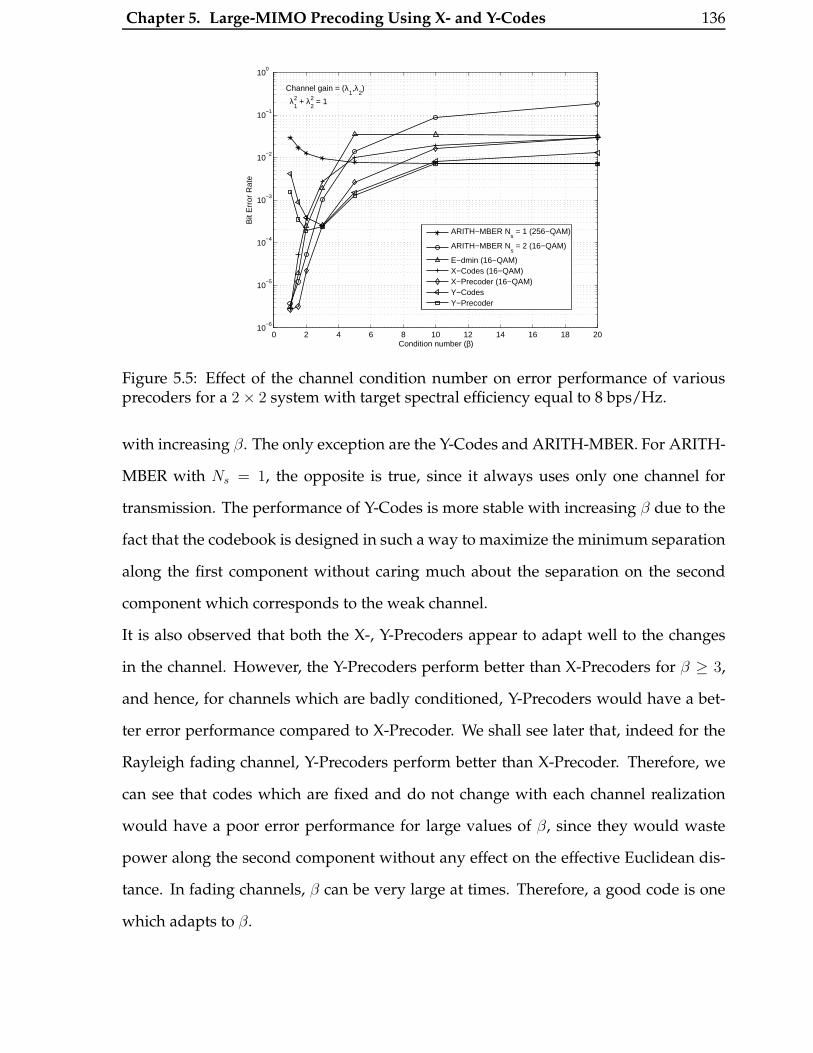
Chapter 5. Large-MIMO Precoding Using X- and Y-Codes 136
0 2 4 6 8 10 12 14 16 18 2010
−6
10−5
10−4
10−3
10−2
10−1
100
Condition number (β)
Bit
Err
or R
ate
ARITH−MBER Ns = 1 (256−QAM)
ARITH−MBER Ns = 2 (16−QAM)
E−dmin (16−QAM)X−Codes (16−QAM)X−Precoder (16−QAM)Y−CodesY−Precoder
Channel gain = (λ1,λ
2)
λ12 + λ
22 = 1
Figure 5.5: Effect of the channel condition number on error performance of variousprecoders for a 2× 2 system with target spectral efficiency equal to 8 bps/Hz.
with increasing β. The only exception are the Y-Codes and ARITH-MBER. For ARITH-
MBER with Ns = 1, the opposite is true, since it always uses only one channel for
transmission. The performance of Y-Codes is more stable with increasing β due to the
fact that the codebook is designed in such a way to maximize the minimum separation
along the first component without caring much about the separation on the second
component which corresponds to the weak channel.
It is also observed that both the X-, Y-Precoders appear to adapt well to the changes
in the channel. However, the Y-Precoders perform better than X-Precoders for β ≥ 3,
and hence, for channels which are badly conditioned, Y-Precoders would have a bet-
ter error performance compared to X-Precoder. We shall see later that, indeed for the
Rayleigh fading channel, Y-Precoders perform better than X-Precoder. Therefore, we
can see that codes which are fixed and do not change with each channel realization
would have a poor error performance for large values of β, since they would waste
power along the second component without any effect on the effective Euclidean dis-
tance. In fading channels, β can be very large at times. Therefore, a good code is one
which adapts to β.

Chapter 5. Large-MIMO Precoding Using X- and Y-Codes 137
We also observe that Y-Codes and Y-Precoders have the best error performance when
channel condition is bad. This justifies the fact that codes for badly conditioned chan-
nels should be designed to have more separation in the minimum distance along the
component corresponding to the stronger channel.
5.5.2 Diversity Order Comparison
We next discuss the diversity order achieved by the various precoding schemes with
Rayleigh fading. Let the number of subchannels used for transmission be Ns (Ns ≤ Nr).
The diversity order achieved by the linear precoders (EE and ARITH-MBER) and THP
is (Nr − Ns + 1)(Nt − Ns + 1) and (Nt − Ns + 1), respectively, whereas the diversity
order achieved by E-dmin and X-, Y-Codes is (Nr− Ns
2+1)(Nt− Ns
2+1). The CI scheme
achieves infinite diversity, but it suffers from power enhancement at the transmitter.
Among all the other schemes (except CI), we observe that E-dmin and X-, Y-Codes
have the best diversity order. The subsequent simulation results assume a Rayleigh
fading channel.
5.5.3 Comparison of BER Performance with Full-rate Transmission
In Fig. 5.6, we plot the BER of all precoders for Nt = Nr = Ns = 2, 4 and a target
spectral efficiency of 2Ns bps/Hz. The proposed X-, Y-Precoders and E-dmin have the
best error performance. The increased diversity order achieved by the pairing scheme
is obvious from the higher slope of the error rate for the X-, Y-Precoders compared to
a slope of order 1 for the linear precoder ARITH-MBER and THP. The performance
of CI is inferior due to enhanced transmit power requirement arising from the bad
conditioning of the channel. It is observed that the proposed Y-Precoders perform the
best for Nt = Nr = 2, with E-dmin only 0.5 dB away at BER of 10−3. For Nt = Nr = 4,
E-dmin performs better than Y-Precoders by 0.4 dB at BER of 10−3. However, E-dmin
has this performance gain at a higher encoding and decoding complexity compared to
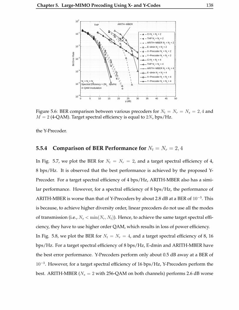
Chapter 5. Large-MIMO Precoding Using X- and Y-Codes 138
0 5 10 15 20 25 30 35 40 45 5010
−6
10−5
10−4
10−3
10−2
10−1
100
γ (dB)
Bit
Err
or R
ate
CI Nr = N
t = 2
THP Nr = N
t = 2
ARITH−MBER Nr = N
t = 2
E−dmin Nr = N
t = 2
X−Precoder Nr = N
t = 2
Y−Precoder Nr = N
t = 2
CI Nr = N
t = 4
THP Nr = N
t = 4
ARITH−MBER Nr = N
t = 4
E−dmin Nr = N
t = 4
X−Precoder Nr = N
t = 4
Y−Precoder Nr = N
t = 4N
r = N
t = N
sSpectral Efficiency = 2N
s bps/Hz
4−QAM modulation
THP ARITH−MBER
Figure 5.6: BER comparison between various precoders for Nt = Nr = Ns = 2, 4 andM = 2 (4-QAM). Target spectral efficiency is equal to 2Ns bps/Hz.
the Y-Precoder.
5.5.4 Comparison of BER Performance for Nt = Nr = 2, 4
In Fig. 5.7, we plot the BER for Nt = Nr = 2, and a target spectral efficiency of 4,
8 bps/Hz. It is observed that the best performance is achieved by the proposed Y-
Precoder. For a target spectral efficiency of 4 bps/Hz, ARITH-MBER also has a simi-
lar performance. However, for a spectral efficiency of 8 bps/Hz, the performance of
ARITH-MBER is worse than that of Y-Precoders by about 2.8 dB at a BER of 10−3. This
is because, to achieve higher diversity order, linear precoders do not use all the modes
of transmission (i.e., Ns < min(Nr, Nt)). Hence, to achieve the same target spectral effi-
ciency, they have to use higher order QAM, which results in loss of power efficiency.
In Fig. 5.8, we plot the BER for Nt = Nr = 4, and a target spectral efficiency of 8, 16
bps/Hz. For a target spectral efficiency of 8 bps/Hz, E-dmin and ARITH-MBER have
the best error performance. Y-Precoders perform only about 0.5 dB away at a BER of
10−3. However, for a target spectral efficiency of 16 bps/Hz, Y-Precoders perform the
best. ARITH-MBER (Ns = 2 with 256-QAM on both channels) performs 2.6 dB worse

Chapter 5. Large-MIMO Precoding Using X- and Y-Codes 139
0 5 10 15 20 25 30 35 40 45 50 5510
−5
10−4
10−3
10−2
10−1
100
γ (dB)
Bit
Err
or R
ate
EE (Ns = 1, 16−QAM)
ARITH−MBER (Ns = 1, 16−QAM)
E−dmin (4−QAM)X−Precoder (4−QAM)Y−Precoder (4 bps/Hz)EE (N
s = 1, 256−QAM)
ARITH−MBER (Ns = 1, 256−QAM)
E−dmin (16−QAM)X−Precoder (16−QAM)Y−Precoder (8 bps/Hz)
Nr = N
t = 2
Spectral Efficiency = 8 bps/HzNr = N
t = 2
Spectral Efficiency = 4 bps/Hz
Figure 5.7: BER comparison between various precoders for Nt = Nr = 2 and targetspectral efficiency = 4, 8 bps/Hz.
0 5 10 15 20 25 30 35 40 45 50 5510
−6
10−5
10−4
10−3
10−2
10−1
100
γ (dB)
Bit
Err
or R
ate
EE (Ns = 2, 16−QAM)
ARITH−MBER (Ns = 2, 16−QAM)
E−dmin (4−QAM)X−Precoder (4−QAM)Y−Precoder (8 bps/Hz)EE (N
s = 2, 256−QAM)
ARITH−MBER (Ns = 2, 256−QAM)
E−dmin (16−QAM)X−Precoder (16−QAM)Y−Precoder (16 bps/Hz)
Nr = N
t = 4
Spectral Efficiency = 8 bps/Hz
Nr = N
t = 4
Spectral Efficiency = 16 bps/Hz
Figure 5.8: BER comparison between various precoders for Nt = Nr = 4 and targetspectral efficiency = 8, 16 bps/Hz.
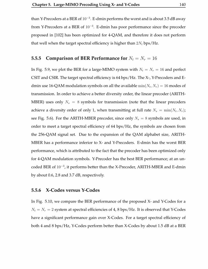
Chapter 5. Large-MIMO Precoding Using X- and Y-Codes 140
than Y-Precoders at a BER of 10−3. E-dmin performs the worst and is about 3.5 dB away
from Y-Precoders at a BER of 10−3. E-dmin has poor performance since the precoder
proposed in [102] has been optimized for 4-QAM, and therefore it does not perform
that well when the target spectral efficiency is higher than 2Nt bps/Hz.
5.5.5 Comparison of BER Performance for Nt = Nr = 16
In Fig. 5.9, we plot the BER for a large-MIMO system with Nt = Nr = 16 and perfect
CSIT and CSIR. The target spectral efficiency is 64 bps/Hz. The X-, Y-Precoders and E-
dmin use 16-QAM modulation symbols on all the available min(Nt, Nr) = 16 modes of
transmission. In order to achieve a better diversity order, the linear precoder (ARITH-
MBER) uses only Ns = 8 symbols for transmission (note that the linear precoders
achieve a diversity order of only 1, when transmitting at full rate Ns = min(Nt, Nr);
see Fig. 5.6). For the ARITH-MBER precoder, since only Ns = 8 symbols are used, in
order to meet a target spectral efficiency of 64 bps/Hz, the symbols are chosen from
the 256-QAM signal set. Due to the expansion of the QAM alphabet size, ARITH-
MBER has a performance inferior to X- and Y-Precoders. E-dmin has the worst BER
performance, which is attributed to the fact that the precoder has been optimized only
for 4-QAM modulation symbols. Y-Precoder has the best BER performance; at an un-
coded BER of 10−3, it performs better than the X-Precoder, ARITH-MBER and E-dmin
by about 0.6, 2.8 and 3.7 dB, respectively.
5.5.6 X-Codes versus Y-Codes
In Fig. 5.10, we compare the BER performance of the proposed X- and Y-Codes for a
Nt = Nr = 2 system at spectral efficiencies of 4, 8 bps/Hz. It is observed that Y-Codes
have a significant performance gain over X-Codes. For a target spectral efficiency of
both 4 and 8 bps/Hz, Y-Codes perform better than X-Codes by about 1.5 dB at a BER
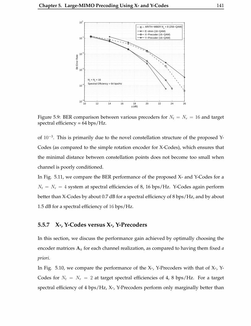
Chapter 5. Large-MIMO Precoding Using X- and Y-Codes 141
10 12 14 16 18 20 22 24 2610
−5
10−4
10−3
10−2
10−1
100
γ (dB)
Bit
Err
or R
ate
ARITH−MBER Ns = 8 (256−QAM)
E−dmin (16−QAM)X−Precoder (16−QAM)Y−Precoder (16−QAM)
Nr = N
t = 16
Spectral Efficiency = 64 bps/Hz
Figure 5.9: BER comparison between various precoders for Nt = Nr = 16 and targetspectral efficiency = 64 bps/Hz.
of 10−3. This is primarily due to the novel constellation structure of the proposed Y-
Codes (as compared to the simple rotation encoder for X-Codes), which ensures that
the minimal distance between constellation points does not become too small when
channel is poorly conditioned.
In Fig. 5.11, we compare the BER performance of the proposed X- and Y-Codes for a
Nt = Nr = 4 system at spectral efficiencies of 8, 16 bps/Hz. Y-Codes again perform
better than X-Codes by about 0.7 dB for a spectral efficiency of 8 bps/Hz, and by about
1.5 dB for a spectral efficiency of 16 bps/Hz.
5.5.7 X-, Y-Codes versus X-, Y-Precoders
In this section, we discuss the performance gain achieved by optimally choosing the
encoder matrices Ak for each channel realization, as compared to having them fixed a
priori.
In Fig. 5.10, we compare the performance of the X-, Y-Precoders with that of X-, Y-
Codes for Nt = Nr = 2 at target spectral efficiencies of 4, 8 bps/Hz. For a target
spectral efficiency of 4 bps/Hz, X-, Y-Precoders perform only marginally better than
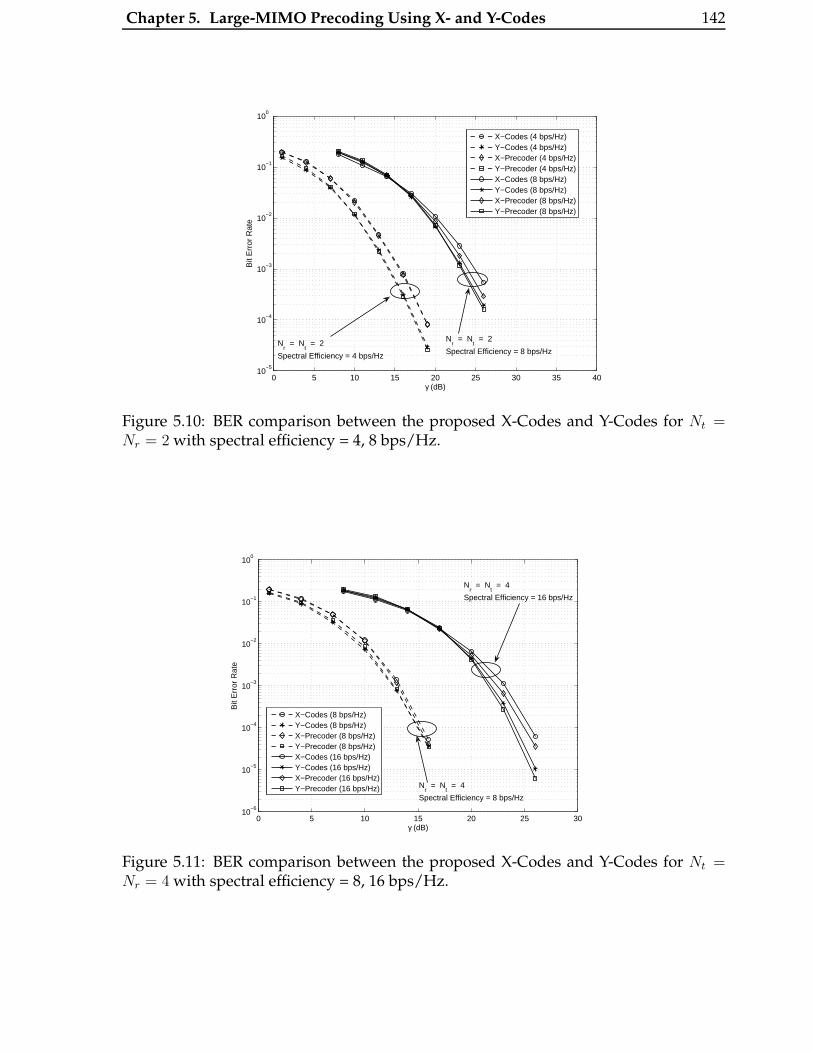
Chapter 5. Large-MIMO Precoding Using X- and Y-Codes 142
0 5 10 15 20 25 30 35 4010
−5
10−4
10−3
10−2
10−1
100
γ (dB)
Bit
Err
or R
ate
X−Codes (4 bps/Hz)Y−Codes (4 bps/Hz)X−Precoder (4 bps/Hz)Y−Precoder (4 bps/Hz)X−Codes (8 bps/Hz)Y−Codes (8 bps/Hz)X−Precoder (8 bps/Hz)Y−Precoder (8 bps/Hz)
Nr = N
t = 2
Spectral Efficiency = 4 bps/Hz
Nr = N
t = 2
Spectral Efficiency = 8 bps/Hz
Figure 5.10: BER comparison between the proposed X-Codes and Y-Codes for Nt =Nr = 2 with spectral efficiency = 4, 8 bps/Hz.
0 5 10 15 20 25 3010
−6
10−5
10−4
10−3
10−2
10−1
100
γ (dB)
Bit
Err
or R
ate
X−Codes (8 bps/Hz)Y−Codes (8 bps/Hz)X−Precoder (8 bps/Hz)Y−Precoder (8 bps/Hz)X−Codes (16 bps/Hz)Y−Codes (16 bps/Hz)X−Precoder (16 bps/Hz)Y−Precoder (16 bps/Hz) N
r = N
t = 4
Spectral Efficiency = 8 bps/Hz
Nr = N
t = 4
Spectral Efficiency = 16 bps/Hz
Figure 5.11: BER comparison between the proposed X-Codes and Y-Codes for Nt =Nr = 4 with spectral efficiency = 8, 16 bps/Hz.

Chapter 5. Large-MIMO Precoding Using X- and Y-Codes 143
X-, Y-Codes (by only about 0.2 dB at a BER of 10−3). However, for a target spectral
efficiency of 8 bps/Hz, the X-Precoder performs better than X-Codes by about 1 dB,
whereas Y-Precoders perform better than Y-Codes by about 0.2 dB at a BER of 10−3.
Therefore, changing the encoder matrices with channel realization is beneficial for X-
Codes. However, it is observed that Y-Precoders do not have as much gain in perfor-
mance compared to Y-Codes.
For Nt = Nr = 4, it is observed from Fig. 5.11 that for a target spectral efficiency of
8 bps/Hz, X-, Y-Precoders have almost similar performances as those of X-, Y-Codes.
However, for a target spectral efficiency of 16 bps/Hz, X-Precoders perform better than
X-Codes by about 0.7 dB, whereas Y-Precoders perform better than Y-Codes by about
0.3 dB at a BER of 10−3.
The performance gain of X-Precoders over X-Codes is much more significant as com-
pared to that of the Y-Precoders over Y-Codes. Also, for X-Precoders, this performance
gain is significant only with higher order QAM. This is due to the fact that the error
performance is much more sensitive to the rotation angle for higher order QAM (see
Fig. 5.2), and therefore adjusting the rotation angle with respect to the varying channel
is expected to result in performance improvement.
On the other hand, Y-Precoders are only marginally better than Y-Codes irrespective of
the spectral efficiency. This is attributed to the fact that for the Y-Precoders we optimize
the upper bound to the probability of error rather than the exact error probability. We
do this, because of the analytical intractability of the exact error probability expression.
This leads to a suboptimal choice of the encoder matrices, and therefore a suboptimal
error performance. This is obvious from Fig. 5.12, where we plot the exact optimal
WEP in comparison with the error probability of the proposed suboptimal Y-Precoder.
The exact optimal WEP (i.e., error probability with the optimal choice of encoder ma-
trices) is computed through Monte Carlo techniques using (5.69) and the integrals in

Chapter 5. Large-MIMO Precoding Using X- and Y-Codes 144
8 10 12 14 16 18 2010
−2
10−1
100
γ (dB)
Wor
d E
rror
Pro
babi
lity
Proposed suboptimal Y−Precoder (Nr = N
t = 2)
Exact Optimal Y−Precoder (Nr = N
t = 2)
Proposed suboptimal Y−Precoder (Nr = N
t = 4)
Exact Optimal Y−Precoder (Nr = N
t = 4)
Spectral Efficiency = 4 Nt bps/Hz
Figure 5.12: Word error probability comparison between the proposed suboptimal Y-Precoders and exact optimal Y-Precoders for Nt = Nr = 2, 4 with spectral efficiency =4Nt bps/Hz.
(5.72). The exact optimal error probability is better than the proposed suboptimal Y-
Precoder by about 1.8 dB for a Nt = Nr = 2 system, and is better by about 1 dB for a
Nt = Nr = 4 system at a WEP of 10−1. This, therefore, suggests the existence of better
Y-Precoders compared to what has been proposed here.
5.6 Complexity
In this section, we discuss the computational complexity of X-, Y-Codes and compare
it with those of other precoding schemes. The linear precoders (ARITH-MBER and
EE), E-dmin and X-Codes need to compute the SVD decomposition of H. The CI and
THP schemes involve computing the pseudo-inverse and QR decomposition of H, re-
spectively. The complexity of computing SVD, QR as well as pseudo-inverse is O(N3r ).
Since the channel is slowly fading, these computations can be performed once, and
can be used until the channel changes. We, therefore, do not consider the complexity
of these decompositions in the discussion below.
Chapter 5. Large-MIMO Precoding Using X- and Y-Codes 145
5.6.1 Encoding Complexity
The encoding complexity of all the schemes is O(NtNr), which is due to the trans-
mit pre-processing filter. If the number of operations were to be computed, CI and
X-, Y-Codes would have the lowest complexity. This is so because linear precoders
need to compute an extra pre-processing matrix (in addition to SVD). THP also has
to do successive interference pre-cancellation (in addition to QR). On the other hand,
E-dmin and X-, Y-Codes need to only compute SVD, which automatically gives the
pre-processing and the post-processing matrices. Also, X-, Y-Codes have lower encod-
ing complexity compared to E-dmin, because the encoding matrices Ak are real, as
opposed to being complex for E-dmin. CI has an even lower complexity since there is
no spatial coding.
5.6.2 Decoding Complexity
The decoding complexity of all the schemes have a square dependence on Nr. This
is due to the post-processing matrix filter at the receiver. The linear precoders, CI
and THP employ post processing at the receiver, which enables independent ML de-
coding for each subchannel. With QAM modulation symbols, this is only a rounding
operation for each subchannel. E-dmin and X-Codes, on the other hand, use sphere
decoding to jointly decode pairs of subchannels. ML decoding for X-Codes is accom-
plished by using Nr 2-dimensional real sphere decoders. However, E-dmin requires
Nr
24-dimensional real sphere decoders. The average complexity of sphere decoding is
cubic in the number of dimensions (and is invariant w.r.t modulation alphabet size M)
[50], and therefore X-Codes have a much lower decoding complexity when compared
to E-dmin. The ML decoding complexity of Y-Codes is independent of M , and is equal
to the ML decoding complexity of a scalar channel. Therefore, the linear precoders,
CI, THP and Y-Codes have the lowest ML decoding complexity among the considered
precoding schemes.

Chapter 5. Large-MIMO Precoding Using X- and Y-Codes 146
Finally, we remark that the good performance and low complexity of the proposed
X-/Y-Codes and X-/Y-Precoders make them well suited for high spectral efficiency
large-MIMO precoding. Further, we will exploit the structure of X-codes to increase
MIMO capacity with discrete input alphabets in the next chapter.
Chapter 6
Precoding with X-codes to Increase
Capacity with Discrete Input Alphabets
In this chapter, we propose a non-diagonal precoder based on the X-Codes proposed in
the previous chapter to increase the mutual information with discrete input alphabet.
Many modern communication channels are modeled as a Gaussian MIMO channel.
Examples include multi-tone digital subscriber line (DSL), orthogonal frequency di-
vision multiplexing (OFDM), and multiple transmit-receive antenna systems. It is
known that the capacity of the Gaussian MIMO channel is achieved by beamform-
ing a Gaussian input alphabet along the right singular vectors of the MIMO channel. The
received vector is projected along the left singular vectors, resulting in a set of parallel
Gaussian subchannels. Optimal power allocation between the subchannels is achieved
by waterfilling [91]. In practice, the input alphabet is not Gaussian and is generally cho-
sen from a finite signal set.
We distinguish between two kinds of MIMO channels: i) diagonal (or parallel) channels
and ii) non-diagonal channels.
For a diagonal MIMO channel with discrete input alphabets, assuming only power
allocation on each subchannel (i.e., a diagonal precoder), Mercury/waterfilling was
shown to be optimal by Lozano et al. in [98]. With discrete input alphabets, Cruz et al.
147

Chapter 6. Precoding with X-codes to Increase Capacity with Discrete Input Alphabets148
later proved in [95] that the optimal precoder is, however, non-diagonal, i.e., precoding
needs to be performed across all the subchannels.
For a general non-diagonal Gaussian MIMO channel, it was also shown in [95] that
the optimal precoder is non-diagonal. Such an optimal precoder is given by a fixed
point equation, which requires a high complexity numeric evaluation. Since the pre-
coder jointly codes all the n inputs, joint decoding is also required at the receiver.
Thus, the decoding complexity can be very high, specially for large n, as in the case
of DSL, OFDM and large-MIMO systems. This motivates our quest for a practical low-
complexity precoding scheme achieving near optimal capacity.
In this chapter, we consider a general MIMO channel and a non-diagonal precoder
based on X-Codes proposed in the previous chapter. The MIMO channel is trans-
formed into a set of parallel subchannels using singular value decomposition (SVD)
and X-Codes are then used to pair the subchannels. X-Codes are fully characterized by
the pairings and the 2-dimensional real rotation matrices for each pair. These rotation
matrices are parameterized with a single angle. This precoding structure enables us
to express the total mutual information as a sum of the mutual information of all the
pairs.
The problem of finding the optimal precoder with the above structure, which maxi-
mizes the total mutual information, can be split into two tractable problems: i) opti-
mizing the rotation angle and the power allocation within each pair, and ii) finding the
optimal pairing and power allocation among the pairs. It is shown that the mutual
information achieved with the proposed pairing scheme is very close to that achieved
with the optimal precoder by Cruz et al. in [95], and is significantly better than the
Mercury/waterfilling strategy by Lozano et al. in [98]. Our approach greatly simplifies
both the precoder optimization and the detection complexity, making it suitable for
practical applications.
The rest of this chapter is organized as follows. Section 6.1 introduces the system

Chapter 6. Precoding with X-codes to Increase Capacity with Discrete Input Alphabets149
model. In Section 6.2, we discuss the optimal precoder with discrete inputs in [95]
and the relevant MIMO capacity. In Section 6.3, we propose a precoding scheme us-
ing X-Codes with discrete inputs and present its relevant capacity. In Section 6.4, we
consider the first problem, which is to find the optimal rotation angle and power alloca-
tion for a given pair. This problem is equivalent to optimizing the mutual information
for a Gaussian MIMO channel with two subchannels. In Section 6.5, using the results
from Section 6.4, we attempt to optimize the mutual information for a Gaussian MIMO
channel with a large number of subchannels (i.e., in a large-MIMO system). In Section
6.6, we discuss the application of our precoding to OFDM and large-MIMO systems.
6.1 System Model and Precoding with Gaussian Inputs
We consider a Nt×Nr MIMO channel, where the CSI is known perfectly at both trans-
mitter and receiver. Let x = (x1, · · · , xNt)T be the vector of input symbols to the chan-
nel, and let H = {hij}, i = 1, · · · , Nr, j = 1, · · · , Nt, be a full rank Nr × Nt channel
coefficient matrix, with hij representing the complex channel gain between the jth in-
put symbol and the ith output symbol. The vector of Nr channel output symbols is
given by
y =√
PTHx + w, (6.1)
where w is an uncorrelated Gaussian noise vector, such that E[wwH ] = INr , and PT is
the total transmitted power. The power constraint is given by
E[‖x‖2] = 1. (6.2)
The maximum multiplexing gain of this channel is n = min(Nt, Nr).
Let u = (u1, · · · , un)T ∈ Cn be the vector of n information symbols to be sent through
the MIMO channel, with E[|ui|2] = 1, i = 1, · · · , n. Then the vector u can be precoded
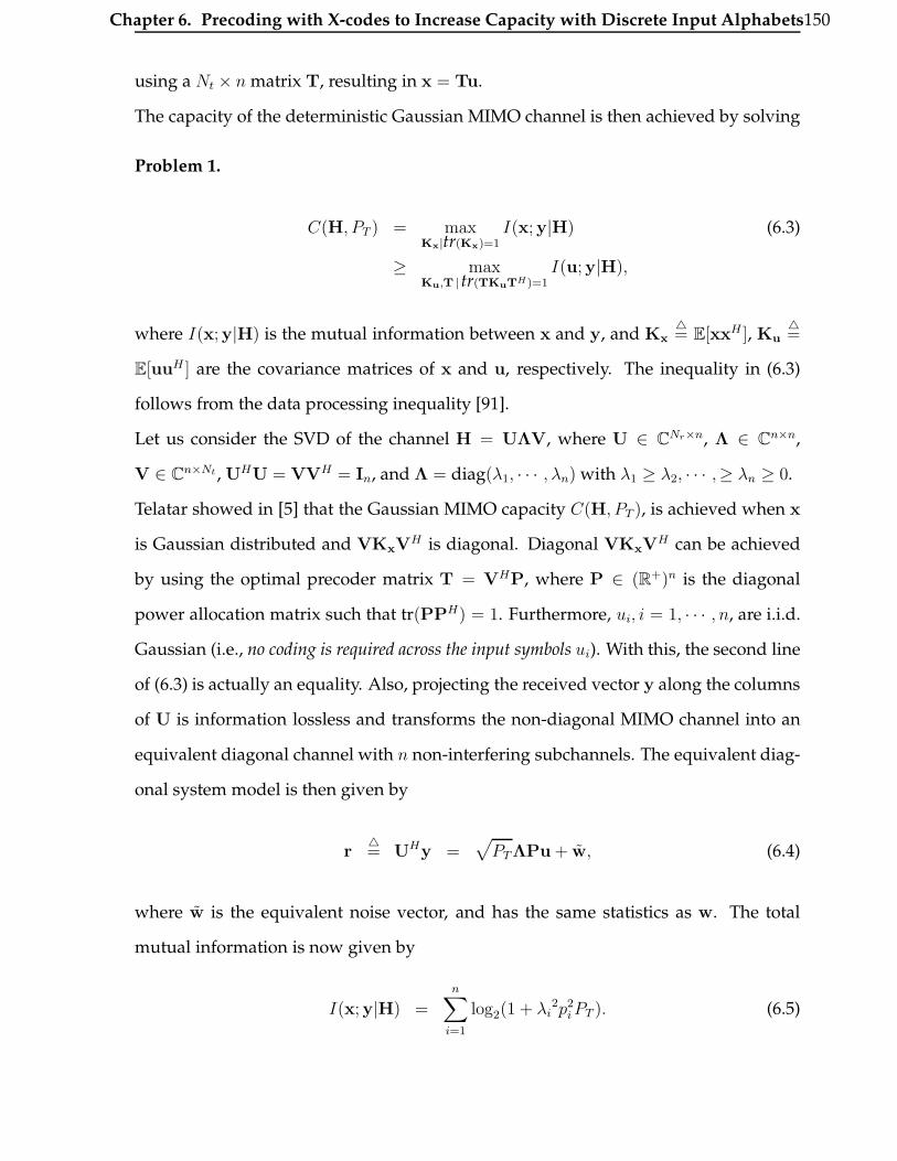
Chapter 6. Precoding with X-codes to Increase Capacity with Discrete Input Alphabets150
using a Nt × n matrix T, resulting in x = Tu.
The capacity of the deterministic Gaussian MIMO channel is then achieved by solving
Problem 1.
C(H, PT ) = maxKx|tr(Kx)=1
I(x;y|H) (6.3)
≥ maxKu,T | tr(TKuTH)=1
I(u;y|H),
where I(x;y|H) is the mutual information between x and y, and Kx
4= E[xxH ], Ku
4=
E[uuH ] are the covariance matrices of x and u, respectively. The inequality in (6.3)
follows from the data processing inequality [91].
Let us consider the SVD of the channel H = UΛV, where U ∈ CNr×n, Λ ∈ Cn×n,
V ∈ Cn×Nt , UHU = VVH = In, and Λ = diag(λ1, · · · , λn) with λ1 ≥ λ2, · · · ,≥ λn ≥ 0.
Telatar showed in [5] that the Gaussian MIMO capacity C(H, PT ), is achieved when x
is Gaussian distributed and VKxVH is diagonal. Diagonal VKxV
H can be achieved
by using the optimal precoder matrix T = VHP, where P ∈ (R+)n is the diagonal
power allocation matrix such that tr(PPH) = 1. Furthermore, ui, i = 1, · · · , n, are i.i.d.
Gaussian (i.e., no coding is required across the input symbols ui). With this, the second line
of (6.3) is actually an equality. Also, projecting the received vector y along the columns
of U is information lossless and transforms the non-diagonal MIMO channel into an
equivalent diagonal channel with n non-interfering subchannels. The equivalent diag-
onal system model is then given by
r4= UHy =
√PTΛPu + w, (6.4)
where w is the equivalent noise vector, and has the same statistics as w. The total
mutual information is now given by
I(x;y|H) =n∑
i=1
log2(1 + λi2p2
i PT ). (6.5)

Chapter 6. Precoding with X-codes to Increase Capacity with Discrete Input Alphabets151
Note that now the mutual information is a function of only the power allocation matrix
P = diag(p1, · · · , pn), with the constraint tr(PPH) = 1. Optimal power allocation is
achieved through waterfilling between the n parallel channels of the equivalent system
in (6.4) [91].
6.2 Optimal Precoding with Discrete Inputs
In practice, discrete input alphabets are used. Subsequently, we assume that the ith
information symbol is given by ui ∈ Ui, where Ui ⊂ C is a finite signal set. Let S 4=
U1 × U2 × · · · × Un be the overall input alphabet. The capacity of the Gaussian MIMO
channel with discrete input alphabet S is defined by the following problem:
Problem 2.
CS(H, PT ) = maxT |u∈S,‖T‖F =1
I(u;y|H). (6.6)
Note that there is no maximization over the pdf of u, since we fix Ku = In. The optimal
precoder Topt, which solves Problem 2, is given by the following fixed point equation
given in [95]:
Topt =HHHToptE
‖HHHToptE‖F, (6.7)
where E is the minimum mean-square error (MMSE) matrix of u given by
E = E[(u− E[u|y])(u− E[u|y])H ]. (6.8)
The optimal precoder is derived using the relation between MMSE and mutual infor-
mation [106]. We observe that, with discrete input alphabets, it is no longer optimal
to beamform along the column vectors of VH and then use waterfilling on the paral-
lel subchannels. Even when H is diagonal (parallel non-interfering subchannels), the
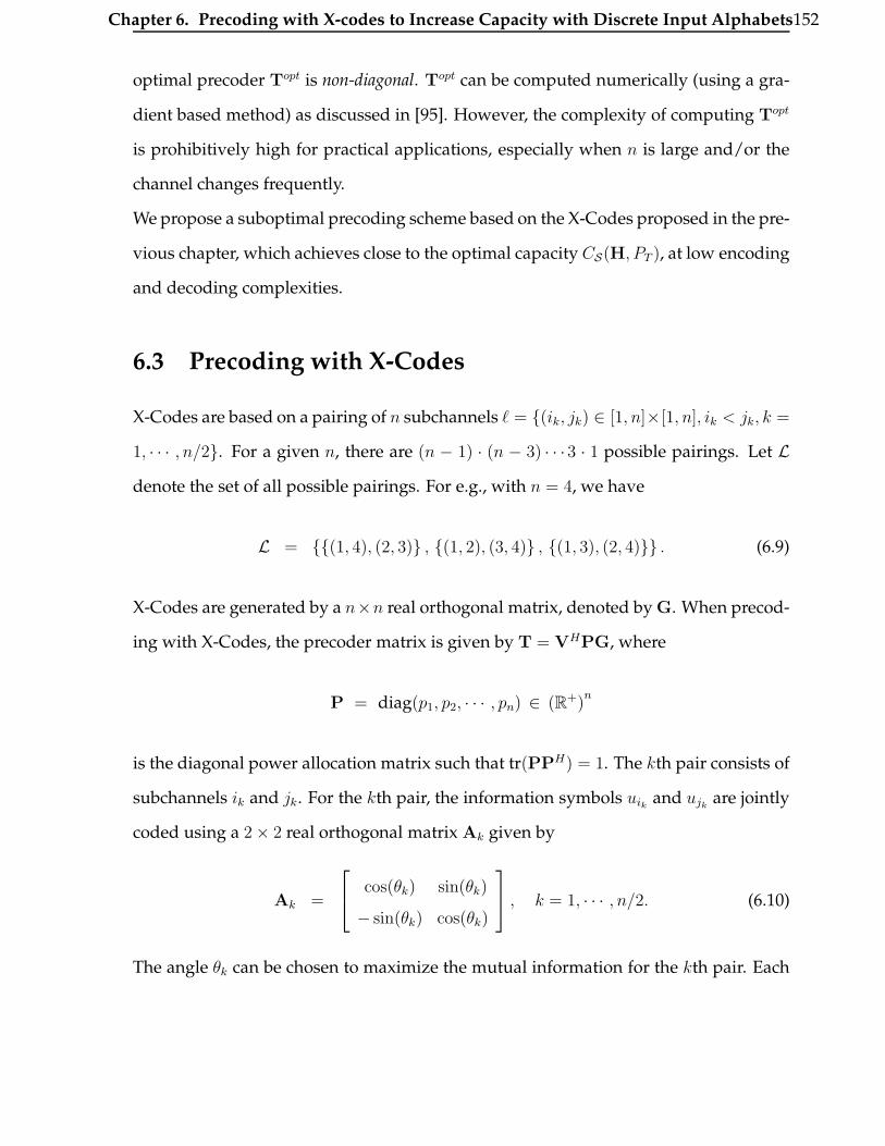
Chapter 6. Precoding with X-codes to Increase Capacity with Discrete Input Alphabets152
optimal precoder Topt is non-diagonal. Topt can be computed numerically (using a gra-
dient based method) as discussed in [95]. However, the complexity of computing Topt
is prohibitively high for practical applications, especially when n is large and/or the
channel changes frequently.
We propose a suboptimal precoding scheme based on the X-Codes proposed in the pre-
vious chapter, which achieves close to the optimal capacity CS(H, PT ), at low encoding
and decoding complexities.
6.3 Precoding with X-Codes
X-Codes are based on a pairing of n subchannels ` = {(ik, jk) ∈ [1, n]×[1, n], ik < jk, k =
1, · · · , n/2}. For a given n, there are (n − 1) · (n − 3) · · ·3 · 1 possible pairings. Let L
denote the set of all possible pairings. For e.g., with n = 4, we have
L = {{(1, 4), (2, 3)} , {(1, 2), (3, 4)} , {(1, 3), (2, 4)}} . (6.9)
X-Codes are generated by a n×n real orthogonal matrix, denoted by G. When precod-
ing with X-Codes, the precoder matrix is given by T = VHPG, where
P = diag(p1, p2, · · · , pn) ∈ (R+)n
is the diagonal power allocation matrix such that tr(PPH) = 1. The kth pair consists of
subchannels ik and jk. For the kth pair, the information symbols uik and ujkare jointly
coded using a 2× 2 real orthogonal matrix Ak given by
Ak =
cos(θk) sin(θk)
− sin(θk) cos(θk)
, k = 1, · · · , n/2. (6.10)
The angle θk can be chosen to maximize the mutual information for the kth pair. Each
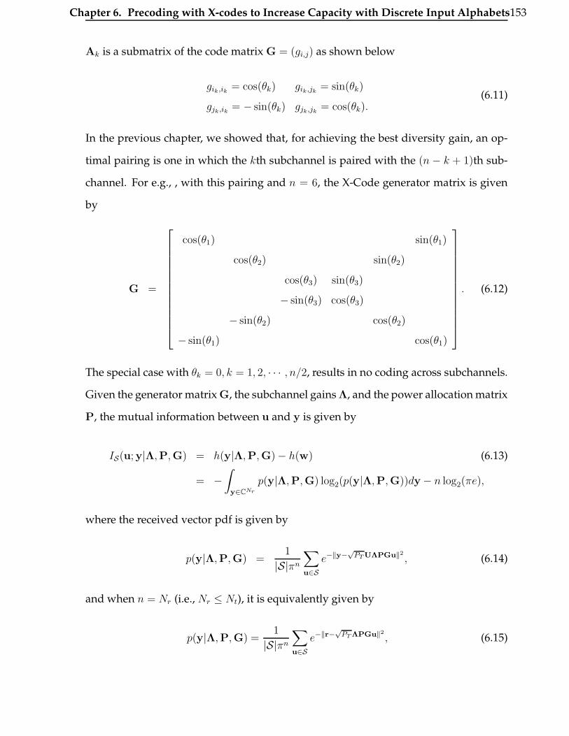
Chapter 6. Precoding with X-codes to Increase Capacity with Discrete Input Alphabets153
Ak is a submatrix of the code matrix G = (gi,j) as shown below
gik,ik = cos(θk) gik,jk= sin(θk)
gjk,ik = − sin(θk) gjk,jk= cos(θk).
(6.11)
In the previous chapter, we showed that, for achieving the best diversity gain, an op-
timal pairing is one in which the kth subchannel is paired with the (n − k + 1)th sub-
channel. For e.g., , with this pairing and n = 6, the X-Code generator matrix is given
by
G =
cos(θ1) sin(θ1)
cos(θ2) sin(θ2)
cos(θ3) sin(θ3)
− sin(θ3) cos(θ3)
− sin(θ2) cos(θ2)
− sin(θ1) cos(θ1)
. (6.12)
The special case with θk = 0, k = 1, 2, · · · , n/2, results in no coding across subchannels.
Given the generator matrix G, the subchannel gains Λ, and the power allocation matrix
P, the mutual information between u and y is given by
IS(u;y|Λ,P,G) = h(y|Λ,P,G)− h(w) (6.13)
= −∫
y∈CNr
p(y|Λ,P,G) log2(p(y|Λ,P,G))dy− n log2(πe),
where the received vector pdf is given by
p(y|Λ,P,G) =1
|S|πn
∑
u∈Se−‖y−
√PT UΛPGu‖2
, (6.14)
and when n = Nr (i.e., Nr ≤ Nt), it is equivalently given by
p(y|Λ,P,G) =1
|S|πn
∑
u∈Se−‖r−
√PT ΛPGu‖2
, (6.15)

Chapter 6. Precoding with X-codes to Increase Capacity with Discrete Input Alphabets154
where r = (r1, r2, · · · , rn)T 4= UHy.
We next define the capacity of the MIMO Gaussian channel when precoding with G.
In the following, we assume that Nr ≤ Nt, so that IS(u;y|Λ,P,G) = IS(u; r|Λ,P,G).
Note that, when Nr > Nt, the receiver processing r = UHy becomes information lossy,
and IS(u;y|Λ,P,G) > IS(u; r|Λ,P,G).
We introduce the following definitions. For a given pairing `, let rk4= (rik , rjk
)T , uk4=
(uik , ujk)T , Λk
4= diag(λik , λjk
), Pk4= diag(pik , pjk
), and Sk4= Uik × Ujk
. Due to the
pairing structure of G the mutual information IS(u; r|Λ,P,G) can be expressed as the
sum of mutual information of all the n/2 pairs as follows:
IS(u; r|Λ,P,G) =
n/2∑
k=1
ISk(uk; rk|Λk,Pk, θk). (6.16)
Having fixed the precoder structure to T = VHPG, we can formulate the following
problem:
Problem 3.
CX(H, PT ) = maxG,P |u∈S,tr(PPH )=1
IS(u; r|Λ,P,G). (6.17)
It is clear that the solution of the above problem is still a formidable task, although it is
simpler than Problem 2. In fact, instead of the n× n variables of T, we now deal with
n variables for power allocation in P, n/2 variables for the angles defining Ak, and the
pairing ` ∈ L. In the following, we will show how to efficiently solve Problem 3 by
splitting it into two simpler problems.
Power allocation can be divided into power allocation among the n/2 pairs, followed
by power allocation between the two subchannels of each pair.
Let P = diag(p1, p2, · · · , pn/2) be a diagonal matrix, where pk4=√
p2ik
+ p2jk
with p2k
being the power allocated to the kth pair. The power allocation within each pair can be
simply expressed in terms of the fraction fk4= p2
ik/p2
k of the power assigned to the first
Chapter 6. Precoding with X-codes to Increase Capacity with Discrete Input Alphabets155
subchannel of the pair. The mutual information achieved by the kth pair is then given
by
ISk(uk; rk|Λk,Pk, θk) = ISk
(uk; rk|Λk, pk, fk, θk) (6.18)
= −∫
rk∈C2
p(rk) log2 p(rk) drk − 2 log2(πe), (6.19)
where p(rk) is given by
p(rk) =1
|Sk|π2
∑
uk∈Sk
e−‖rk−√
PT pkΛkFkAkuk‖2
, (6.20)
where Fk4= diag(
√fk,√
1− fk) and Ak is given by (6.10).
The capacity of the discrete input MIMO Gaussian channel when precoding with X-
Codes can be expressed as
Problem 4.
CX(H, PT ) = max`∈L,P|tr(PPH)=1
n/2∑
k=1
CSk(k, `, pk), (6.21)
where CSk(k, `, pk), the capacity of the kth pair in the pairing `, is achieved by solving
Problem 5.
CSk(k, `, pk) = max
θk,fk
ISk(uk; rk|Λk, pk, fk, θk). (6.22)
In other words, we have split Problem 3 into two different simpler problems. Firstly,
given a pairing ` and power allocation between pairs P, we can solve Problem 5 for
each k = 1, 2, · · · , n/2. Problem 4 uses the solution to Problem 5 to find the optimal
pairing `opt and the optimal power allocation Popt between the n/2 pairs. For small
n, the optimal pairing and power allocation between pairs can always be computed
numerically and by brute force enumeration of all possible pairings. This is, however,
Chapter 6. Precoding with X-codes to Increase Capacity with Discrete Input Alphabets156
prohibitively complex for large n, and we shall discuss heuristic approaches in Section
6.5.
We will show in the following that, although suboptimal, precoding with X-Codes
will provide a close to optimal capacity with the additional benefit that the detection
complexity at the receiver is highly reduced, since there is coupling only between pairs
of channels, as compared to the case of full-coupling for the optimal precoder in [95].
In the next section, we solve Problem 5, which is equivalent to finding the optimal
rotation angle and power allocation for a Gaussian MIMO channel with only n = 2
subchannels.
6.4 Gaussian MIMO Channels with n = 2
With n = 2, there is only one pair and only one possible pairing. Therefore, we drop
the subscript k in Problem 5 and find CX(H, PT ) in Problem 3. The processed received
vector r ∈ C2 is given by
r =√
PTΛFAu + z (6.23)
where z = UHw is the equivalent noise vector with the same statistics as w. Let α4=
λ21 + λ2
2 be the overall channel power gain and β4= λ1/λ2 be the condition number of the
channel. Then (6.23) can be re-written as
r =
√PT ΛFAu + z, (6.24)
where PT4= PT α and Λ
4= Λ/
√α = diag(β/
√1 + β2, 1/
√1 + β2). The equivalent
channel Λ now has a gain of 1, and its channel gains are dependent only upon β.
Our goal is, therefore, to find the optimal rotation angle θopt and the fractional power
allocation f opt, which maximize the mutual information of the equivalent channel with
condition number β and gain α = 1. The total available transmit power is now PT .
Chapter 6. Precoding with X-codes to Increase Capacity with Discrete Input Alphabets157
It is difficult to get analytic expressions for the optimal θopt and f opt, and therefore
we can use numerical techniques to evaluate them and store them in look-up tables
to be used at run time. For a given application scenario, given the distribution of
β, we decide upon a few discrete values of β which are representative of the actual
values observed in real channels. For each such quantized value of β, we numerically
compute a table of the optimal values f opt and θopt as a function of PT . These tables are
constructed off-line. During the process of communication, the transmitter knows the
value of α and β from channel measurements. It then finds the look-up table with the
closest value of β to the measured one. The optimal values f opt and θopt are then found
by indexing the appropriate entry in the table with PT equal to PT α.
In Fig. 6.1, we plot the optimal power fraction f opt to be allocated to the stronger chan-
nel in the pair, as a function of PT . The input alphabet is 16-QAM and β = 1, 1.5, 2, 4, 8.
For β = 1, both channels have equal gains, and therefore, as expected, the optimal
power allocation is to divide power equally between the two subchannels. However,
with increasing β, the power allocation becomes more asymmetrical. It is observed
that at low PT , it is optimal to allocate all power to the stronger channel. At high PT ,
the opposite is true, and it is the weaker channel which gets most of the power. For
a fixed β, as PT increases, the power allocated to the stronger channel is shifted to the
weaker channel. For a fixed PT , a higher fraction of the total power is allocated to the
weaker channel with increasing β. In the high PT regime, these results are in contrast
with the waterfilling scheme, where almost all subchannels are allocated equal power.
In Fig. 6.2, the optimal rotation angle θopt is plotted as a function of PT . The input
alphabet is 16-QAM and β = 1, 1.5, 2, 4, 8. For β = 1, it is observed that the mutual
information is independent of θ for all values of PT . For β = 1.5, 2, the optimal rotation
angle is almost invariant to PT . For larger β, the optimal rotation angle varies with PT
and approximately ranges between 30− 40◦ for all PT values of interest.
Figure 6.3 shows the variation of the mutual information with the power fraction f for

Chapter 6. Precoding with X-codes to Increase Capacity with Discrete Input Alphabets158
0 5 10 15 20 25 300.1
0.2
0.3
0.4
0.5
0.6
0.7
0.8
0.9
1
PT (dB)
Opt
imal
Pow
er A
lloca
tion
Fra
ctio
n (
f opt
)
β = 1β = 1.5β = 2β = 4β = 8
n = 2, 16−QAM, α = 1
Figure 6.1: Plot of f opt versus PT for n = 2 parallel channels with β = 1, 1.5, 2, 4, 8 andα = 1. Input alphabet is 16-QAM.
5 10 15 20 25
30
32
34
36
38
40
42
44
46
PT (dB)
θ o
pt (
deg)
β = 1.5
β = 2
β = 4
β = 8n = 2, 16−QAM, α = 1
Figure 6.2: Plot of θopt versus PT for n = 2 parallel channels with β = 1.5, 2, 4, 8 andα = 1. Input alphabet is 16-QAM.
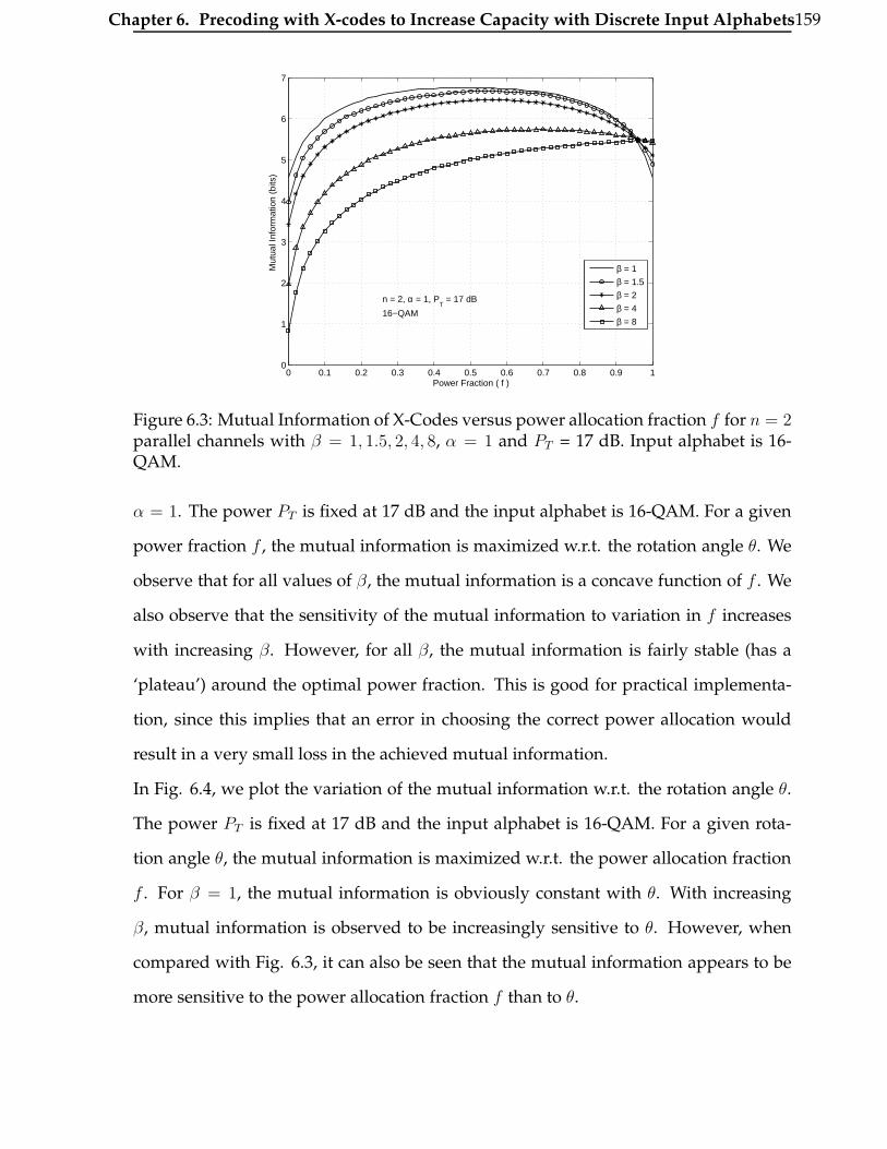
Chapter 6. Precoding with X-codes to Increase Capacity with Discrete Input Alphabets159
0 0.1 0.2 0.3 0.4 0.5 0.6 0.7 0.8 0.9 10
1
2
3
4
5
6
7
Power Fraction ( f )
Mut
ual I
nfor
mat
ion
(bits
)
β = 1
β = 1.5
β = 2
β = 4
β = 8
n = 2, α = 1, PT = 17 dB
16−QAM
Figure 6.3: Mutual Information of X-Codes versus power allocation fraction f for n = 2parallel channels with β = 1, 1.5, 2, 4, 8, α = 1 and PT = 17 dB. Input alphabet is 16-QAM.
α = 1. The power PT is fixed at 17 dB and the input alphabet is 16-QAM. For a given
power fraction f , the mutual information is maximized w.r.t. the rotation angle θ. We
observe that for all values of β, the mutual information is a concave function of f . We
also observe that the sensitivity of the mutual information to variation in f increases
with increasing β. However, for all β, the mutual information is fairly stable (has a
‘plateau’) around the optimal power fraction. This is good for practical implementa-
tion, since this implies that an error in choosing the correct power allocation would
result in a very small loss in the achieved mutual information.
In Fig. 6.4, we plot the variation of the mutual information w.r.t. the rotation angle θ.
The power PT is fixed at 17 dB and the input alphabet is 16-QAM. For a given rota-
tion angle θ, the mutual information is maximized w.r.t. the power allocation fraction
f . For β = 1, the mutual information is obviously constant with θ. With increasing
β, mutual information is observed to be increasingly sensitive to θ. However, when
compared with Fig. 6.3, it can also be seen that the mutual information appears to be
more sensitive to the power allocation fraction f than to θ.
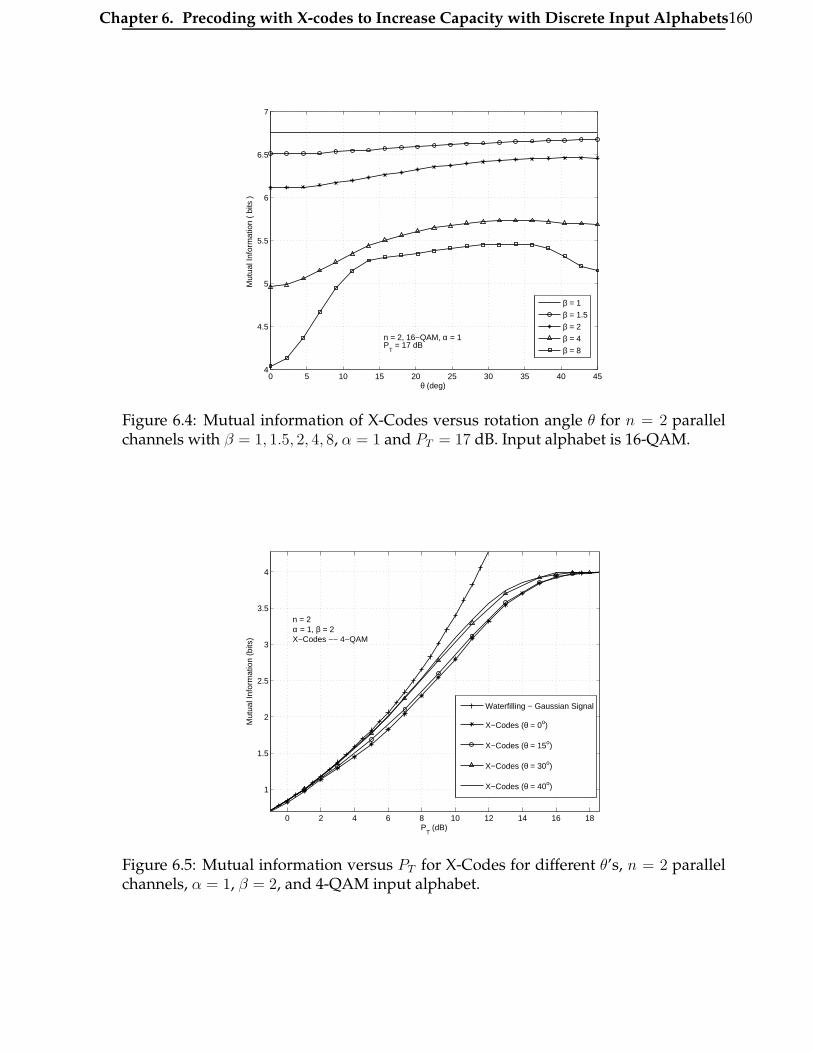
Chapter 6. Precoding with X-codes to Increase Capacity with Discrete Input Alphabets160
0 5 10 15 20 25 30 35 40 454
4.5
5
5.5
6
6.5
7
θ (deg)
Mut
ual I
nfor
mat
ion
( bi
ts )
β = 1
β = 1.5
β = 2
β = 4
β = 8
n = 2, 16−QAM, α = 1P
T = 17 dB
Figure 6.4: Mutual information of X-Codes versus rotation angle θ for n = 2 parallelchannels with β = 1, 1.5, 2, 4, 8, α = 1 and PT = 17 dB. Input alphabet is 16-QAM.
0 2 4 6 8 10 12 14 16 18
1
1.5
2
2.5
3
3.5
4
PT (dB)
Mut
ual I
nfor
mat
ion
(bits
)
Waterfilling − Gaussian Signal
X−Codes (θ = 0o)
X−Codes (θ = 15o)
X−Codes (θ = 30o)
X−Codes (θ = 40o)
n = 2α = 1, β = 2X−Codes −− 4−QAM
Figure 6.5: Mutual information versus PT for X-Codes for different θ’s, n = 2 parallelchannels, α = 1, β = 2, and 4-QAM input alphabet.

Chapter 6. Precoding with X-codes to Increase Capacity with Discrete Input Alphabets161
0 5 10 15 20 250
1
2
3
4
5
6
7
8
9
PT (dB)
Mut
ual I
nfor
mat
ion
(bits
)
Waterfilling − Gaussian Signal
Waterfilling − 4−QAM
Mercury/waterfilling − 4−QAM
X−Codes − 4−QAM
Waterfilling − 16−QAM
Mercury/waterfilling − 16−QAM
X−Codes − 16−QAM
n = 2α = λ
12 + λ
22 = 1
β = 2
Figure 6.6: Mutual information versus PT for n = 2 parallel channels with β = 2 andα = 1, for 4-QAM and 16-QAM.
In Fig. 6.5, we plot the mutual information of X-Codes for different rotation angles
with α = 1 and β = 2. For each rotation angle, the power allocation is optimized
numerically. We observe that the mutual information is quite sensitive to the rotation
angle except in the range 30-40◦.
We next present some simulation results to show that indeed our simple precoding
scheme can significantly increase the mutual information, compared to the case of no
precoding across subchannels (i.e., Mercury/waterfilling). For the sake of compari-
son, we also present the mutual information achieved by the waterfilling scheme with
discrete input alphabets.
We restrict the discrete input alphabets Ui, i = 1, 2, to be square M-QAM alphabets
consisting of two√
M -PAM alphabets in quadrature. Mutual information is evaluated
by solving Problem 5 (i.e., numerically maximizing w.r.t. the rotation angle and power
allocation).
In Fig. 6.6, we plot the maximal mutual information versus PT , for a system with
two subchannels, β = 2 and α = 1. Mutual information is plotted for 4- and 16-
QAM signal sets. It is observed that for a given achievable mutual information, coding

Chapter 6. Precoding with X-codes to Increase Capacity with Discrete Input Alphabets162
−5 0 5 10 15 20 250
0.5
1
1.5
2
2.5
3
3.5
4
PT (dB)
Mut
ual I
nfor
mat
ion
(bits
)
Mercury/waterfilling − β = 1
X−Codes − β = 1
Mercury/waterfilling − β = 2
X−Codes − β = 2
Mercury/waterfilling − β = 4
X−Codes − β = 4
n = 2, 4−QAMα = 1
β = 1
β = 2
β = 4
Figure 6.7: Mutual information versus PT for n = 2 parallel channels with varyingβ = 1, 2, 4, α = 1 and 4-QAM input alphabet.
across subchannels is more power efficient. For e.g., with 4-QAM and an achievable
mutual information of 3 bits, X-Codes require only 0.8 dB more transmit power when
compared to the ideal Gaussian signaling with waterfilling. This gap increases to 1.9
dB for Mercury/waterfilling and 2.8 dB for the waterfilling scheme with 4-QAM as
the input alphabet. A similar trend is observed with 16-QAM as the input alphabet.
The proposed precoder clearly performs better than Mercury/waterfilling, since the
mutual information is optimized w.r.t. the rotation angle θ and power allocation, while
Mercury/waterfilling, as a special case of X-Code, only optimizes power allocation and
fixes θ = 0.
In Fig. 6.7, we compare the mutual information achieved by X-Codes and the Mer-
cury/waterfilling strategy for α = 1 and β = 1, 2, 4. The input alphabet is 4-QAM.
It is observed that both the schemes have the same mutual information when β = 1.
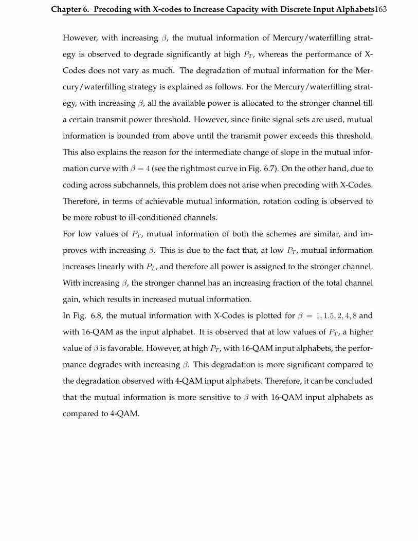
Chapter 6. Precoding with X-codes to Increase Capacity with Discrete Input Alphabets163
However, with increasing β, the mutual information of Mercury/waterfilling strat-
egy is observed to degrade significantly at high PT , whereas the performance of X-
Codes does not vary as much. The degradation of mutual information for the Mer-
cury/waterfilling strategy is explained as follows. For the Mercury/waterfilling strat-
egy, with increasing β, all the available power is allocated to the stronger channel till
a certain transmit power threshold. However, since finite signal sets are used, mutual
information is bounded from above until the transmit power exceeds this threshold.
This also explains the reason for the intermediate change of slope in the mutual infor-
mation curve with β = 4 (see the rightmost curve in Fig. 6.7). On the other hand, due to
coding across subchannels, this problem does not arise when precoding with X-Codes.
Therefore, in terms of achievable mutual information, rotation coding is observed to
be more robust to ill-conditioned channels.
For low values of PT , mutual information of both the schemes are similar, and im-
proves with increasing β. This is due to the fact that, at low PT , mutual information
increases linearly with PT , and therefore all power is assigned to the stronger channel.
With increasing β, the stronger channel has an increasing fraction of the total channel
gain, which results in increased mutual information.
In Fig. 6.8, the mutual information with X-Codes is plotted for β = 1, 1.5, 2, 4, 8 and
with 16-QAM as the input alphabet. It is observed that at low values of PT , a higher
value of β is favorable. However, at high PT , with 16-QAM input alphabets, the perfor-
mance degrades with increasing β. This degradation is more significant compared to
the degradation observed with 4-QAM input alphabets. Therefore, it can be concluded
that the mutual information is more sensitive to β with 16-QAM input alphabets as
compared to 4-QAM.
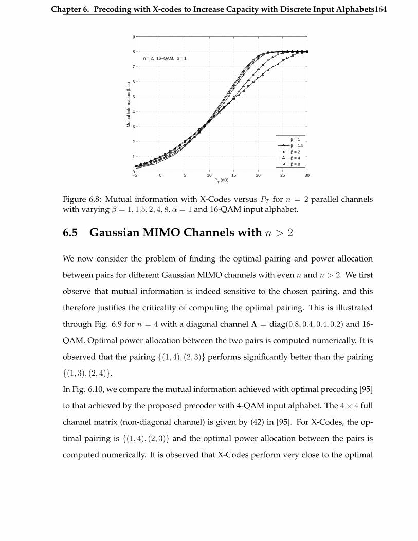
Chapter 6. Precoding with X-codes to Increase Capacity with Discrete Input Alphabets164
−5 0 5 10 15 20 25 300
1
2
3
4
5
6
7
8
9
PT (dB)
Mut
ual I
nfor
mat
ion
(bits
)
β = 1
β = 1.5
β = 2
β = 4
β = 8
n = 2, 16−QAM, α = 1
Figure 6.8: Mutual information with X-Codes versus PT for n = 2 parallel channelswith varying β = 1, 1.5, 2, 4, 8, α = 1 and 16-QAM input alphabet.
6.5 Gaussian MIMO Channels with n > 2
We now consider the problem of finding the optimal pairing and power allocation
between pairs for different Gaussian MIMO channels with even n and n > 2. We first
observe that mutual information is indeed sensitive to the chosen pairing, and this
therefore justifies the criticality of computing the optimal pairing. This is illustrated
through Fig. 6.9 for n = 4 with a diagonal channel Λ = diag(0.8, 0.4, 0.4, 0.2) and 16-
QAM. Optimal power allocation between the two pairs is computed numerically. It is
observed that the pairing {(1, 4), (2, 3)} performs significantly better than the pairing
{(1, 3), (2, 4)}.
In Fig. 6.10, we compare the mutual information achieved with optimal precoding [95]
to that achieved by the proposed precoder with 4-QAM input alphabet. The 4× 4 full
channel matrix (non-diagonal channel) is given by (42) in [95]. For X-Codes, the op-
timal pairing is {(1, 4), (2, 3)} and the optimal power allocation between the pairs is
computed numerically. It is observed that X-Codes perform very close to the optimal

Chapter 6. Precoding with X-codes to Increase Capacity with Discrete Input Alphabets165
0 5 10 15 20 250
2
4
6
8
10
12
14
16
PT (dB)
Mut
ual I
nfor
mat
ion
(bits
)
Waterfilling −− Gaussian Signal
Mercury/waterfilling −− 16−QAM
X−Codes (0.8,0.4),(0.4,0.2) −− 16−QAM
X−Codes (0.8,0.2),(0.4,0.4) −− 16−QAM
n = 4 subchannels, 16−QAMchannel gain = (0.8,0.4,0.4,0.2)
Figure 6.9: Mutual information versus PT with two different pairings for a n = 4 diag-onal channel and 16-QAM input alphabet.
0 5 10 152
3
4
5
6
7
8
PT (dB)
Mut
ual I
nfor
mat
ion
(bits
)
Waterfilling −− GaussianMercury/waterfilling −− 4−QAMOptimal Precoding (Full G) −− 4−QAMX−Codes −− 4−QAM
Figure 6.10: Mutual information versus PT for the Gigabit DSL channel given by (42)in [95].

Chapter 6. Precoding with X-codes to Increase Capacity with Discrete Input Alphabets166
0 5 10 15 202
4
6
8
10
12
14
16
PT (dB)
Mut
ual I
nfor
mat
ion
(bits
)
Waterfilling, 16−QAMMercury/waterfilling, 16−QAMX−Codes, 16−QAMWaterfilling, Gaussian
Ergodic Capacity of4 X 4 Wireless MIMO
Figure 6.11: Comparison of 4 × 4 wireless MIMO ergodic capacity with perfectCSIT/CSIR for 16-QAM input alphabet.
precoding scheme. Specifically, for an achievable mutual information of 6 bits, com-
pared to the optimal precoder [95], X-Codes need only 0.4 dB extra power, whereas 2.3
dB extra power is required with Mercury/waterfilling.
Another application is in wireless MIMO channels with perfect CSI at both the trans-
mitter and the receiver. The channel coefficients are modeled as i.i.d complex normal
random variables with unit variance.
In Fig. 6.11, we plot the ergodic capacity (i.e., the mutual information averaged over
channel realizations) for a 4 × 4 wireless MIMO channel with 16-QAM as the input
alphabet. For X-Codes, the best pairing and power allocation between pairs are chosen
numerically using the optimal θ and power fraction tables created off-line. It is ob-
served that at high PT , simple rotation based coding using X-Codes improves the mu-
tual information significantly, when compared to Mercury/waterfilling. For e.g., for a
target mutual information of 12 bits, X-Codes perform 1.2 dB away from the idealistic
Gaussian signaling scheme. This gap from the Gaussian signaling scheme increases to
3.1 dB for the Mercury/waterfilling scheme and to 4.4 dB for the waterfilling scheme
with 16-QAM alphabet.
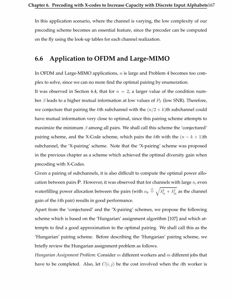
Chapter 6. Precoding with X-codes to Increase Capacity with Discrete Input Alphabets167
In this application scenario, where the channel is varying, the low complexity of our
precoding scheme becomes an essential feature, since the precoder can be computed
on the fly using the look-up tables for each channel realization.
6.6 Application to OFDM and Large-MIMO
In OFDM and Large-MIMO applications, n is large and Problem 4 becomes too com-
plex to solve, since we can no more find the optimal pairing by enumeration.
It was observed in Section 6.4, that for n = 2, a larger value of the condition num-
ber β leads to a higher mutual information at low values of PT (low SNR). Therefore,
we conjecture that pairing the kth subchannel with the (n/2 + k)th subchannel could
have mutual information very close to optimal, since this pairing scheme attempts to
maximize the minimum β among all pairs. We shall call this scheme the ‘conjectured’
pairing scheme, and the X-Code scheme, which pairs the kth with the (n − k + 1)th
subchannel, the ‘X-pairing’ scheme. Note that the ‘X-pairing’ scheme was proposed
in the previous chapter as a scheme which achieved the optimal diversity gain when
precoding with X-Codes.
Given a pairing of subchannels, it is also difficult to compute the optimal power allo-
cation between pairs P. However, it was observed that for channels with large n, even
waterfilling power allocation between the pairs (with αk4=√
λ2ik
+ λ2jk
as the channel
gain of the kth pair) results in good performance.
Apart from the ‘conjectured’ and the ‘X-pairing’ schemes, we propose the following
scheme which is based on the ‘Hungarian’ assignment algorithm [107] and which at-
tempts to find a good approximation to the optimal pairing. We shall call this as the
‘Hungarian’ pairing scheme. Before describing the ‘Hungarian’ pairing scheme, we
briefly review the Hungarian assignment problem as follows.
Hungarian Assignment Problem: Consider m different workers and m different jobs that
have to be completed. Also, let C(i, j) be the cost involved when the ith worker is

Chapter 6. Precoding with X-codes to Increase Capacity with Discrete Input Alphabets168
assigned to the jth job. We can therefore think of a cost matrix, whose (i, j)th entry
has the value C(i, j). The Hungarian assignment problem, is to then find the optimal
assignment of workers to jobs (each worker getting assigned to exactly one job) such
that the total cost of getting all the jobs completed is minimized. It is easy to see, that
a maximization job assignment problem could be posed into a minimization problem
and vice versa.
To find a good approximation to the optimal pairing, we split the n subchannels into
two groups i) Group-I: subchannels 1 to n/2, with the jth subchannel in the role of the
jth job (j = 1, 2, · · · , n/2), ii) Group-II: subchannels n/2 + 1 to n, with the (n/2 + i)th
subchannel in the role of the ith worker (i = 1, 2, · · · , n/2). Therefore, there are n/2
workers and jobs. For a given SNR PT , we initially assume uniform power allocation
between all pairs, and therefore assign a power of 2PT /n to each pair. The value of
C(i, j) is evaluated by finding the optimal mutual information achieved by an equiva-
lent n = 2 channel with the (n/2+ i)th and the jth subchannels as its two subchannels.
This can be obtained by first choosing a table (see Section 6.4) with the closest value of β
to the given λj/λn/2+i, and then indexing the appropriate entry into the table with SNR
= 2PT (λ2j +λ2
n/2+i)/n. The Hungarian algorithm then finds the pairing with the highest
mutual information. Power allocation between the pairs is then achieved through the
waterfilling scheme.
It was observed through Monte-Carlo simulations that, even uniform power alloca-
tion between the subchannels results in almost same mutual information as achieved
through waterfilling between pairs. This can be explained from the fact that by separat-
ing into a group of stronger (Group-I) and a group of weaker channels (Group-II), any
pairing would result in all pairs having almost the same channel gain αk. This therefore
implies that the optimal power allocation scheme would allocate nearly equal power to
all pairs, which both the uniform and the waterfilling schemes would also do. Hence-
forth, it can be conjectured that with the proposed separation of subchannels into 2

Chapter 6. Precoding with X-codes to Increase Capacity with Discrete Input Alphabets169
15 20 25 30 3520
30
40
50
60
70
80
90
100
110
120
SNR per sub carrier (dB)
Tot
al M
utua
l Inf
orm
atio
n (b
its)
Waterfilling, GaussianWaterfilling, 16−QAMMercury/waterfilling, 16−QAMX−Codes X−pairing, 16−QAMX−Codes Hungarian pairing, 16−QAM
OFDM, 32 sub carriersChannel Response Length = 5Bit Loading : 16−QAM per sub carrier
Figure 6.12: Mutual information versus per subcarrier SNR for an OFDM system with32 carriers. X-Codes versus Mercury/waterfilling.
groups, both the uniform and the waterfilling power allocation schemes would have
close to optimal performance, and any further improvement in mutual information by
optimizing the power allocation would be minimal. This also supports the initial usage
of uniform power 2PT /n to compute the entries C(i, j) before executing the Hungarian
algorithm. Furthermore, the computational complexity of the Hungarian algorithm is
O(n3) and is therefore practically feasible.
To study the sensitivity of the mutual information to the pairing of subchannels, we
also consider a ‘Random’ pairing scheme. In the ‘Random’ pairing scheme, we first
choose a large number (≈ 50) of random pairings. For each chosen random pairing, we
evaluate the mutual information (through Monte-Carlo simulations) with waterfilling
power allocation between pairs. Finally, the average mutual information is computed.
This gives us insight into the mean value of the mutual information w.r.t. pairing. It
would also help us in quantifying the effectiveness of the heuristic pairing schemes
discussed above.
Performance in a 32-subcarrier OFDM system: We next illustrate the mutual information
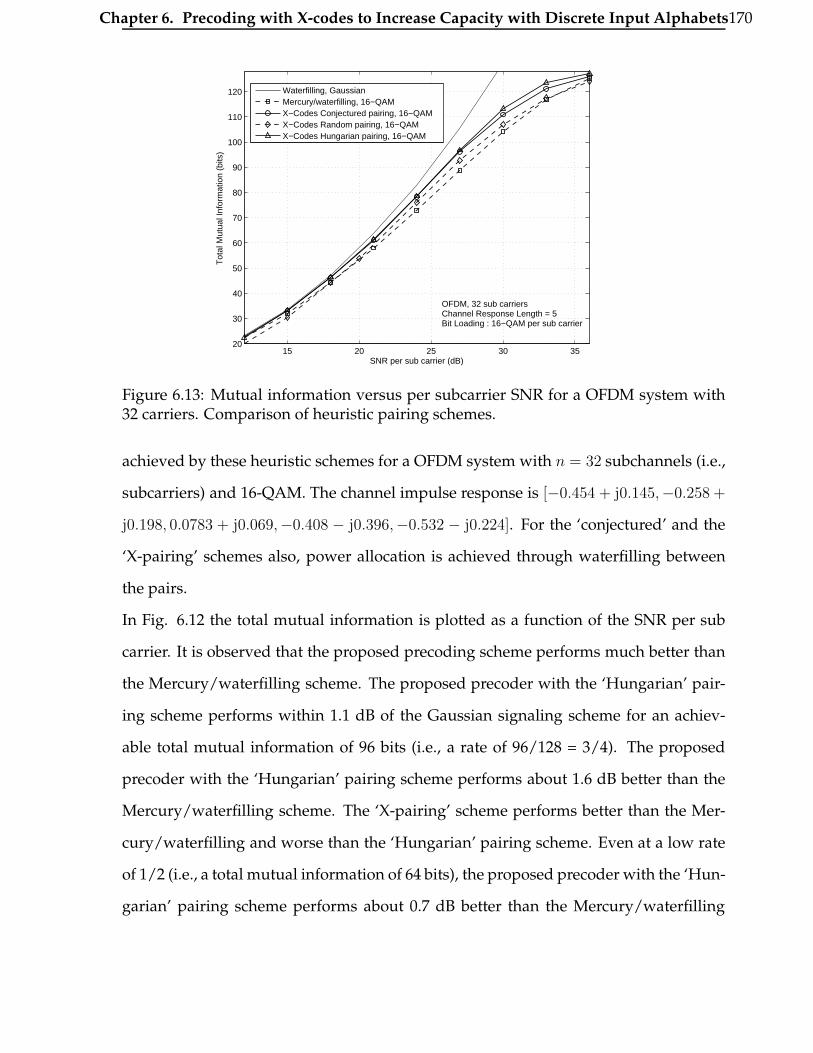
Chapter 6. Precoding with X-codes to Increase Capacity with Discrete Input Alphabets170
15 20 25 30 3520
30
40
50
60
70
80
90
100
110
120
SNR per sub carrier (dB)
Tot
al M
utua
l Inf
orm
atio
n (b
its)
Waterfilling, GaussianMercury/waterfilling, 16−QAMX−Codes Conjectured pairing, 16−QAMX−Codes Random pairing, 16−QAMX−Codes Hungarian pairing, 16−QAM
OFDM, 32 sub carriersChannel Response Length = 5Bit Loading : 16−QAM per sub carrier
Figure 6.13: Mutual information versus per subcarrier SNR for a OFDM system with32 carriers. Comparison of heuristic pairing schemes.
achieved by these heuristic schemes for a OFDM system with n = 32 subchannels (i.e.,
subcarriers) and 16-QAM. The channel impulse response is [−0.454 + j0.145,−0.258 +
j0.198, 0.0783 + j0.069,−0.408 − j0.396,−0.532 − j0.224]. For the ‘conjectured’ and the
‘X-pairing’ schemes also, power allocation is achieved through waterfilling between
the pairs.
In Fig. 6.12 the total mutual information is plotted as a function of the SNR per sub
carrier. It is observed that the proposed precoding scheme performs much better than
the Mercury/waterfilling scheme. The proposed precoder with the ‘Hungarian’ pair-
ing scheme performs within 1.1 dB of the Gaussian signaling scheme for an achiev-
able total mutual information of 96 bits (i.e., a rate of 96/128 = 3/4). The proposed
precoder with the ‘Hungarian’ pairing scheme performs about 1.6 dB better than the
Mercury/waterfilling scheme. The ‘X-pairing’ scheme performs better than the Mer-
cury/waterfilling and worse than the ‘Hungarian’ pairing scheme. Even at a low rate
of 1/2 (i.e., a total mutual information of 64 bits), the proposed precoder with the ‘Hun-
garian’ pairing scheme performs about 0.7 dB better than the Mercury/waterfilling
Chapter 6. Precoding with X-codes to Increase Capacity with Discrete Input Alphabets171
scheme.
In Fig. 6.13, we compare the mutual information achieved by the various heuristic pair-
ing schemes. It is observed that the ‘conjectured’ pairing scheme performs very close
to the ‘Hungarian’ pairing scheme except at very high SNR. For e.g., even for a high
mutual information of 96 bits, the ‘Hungarian’ pairing scheme performs better than the
‘conjectured’ pairing scheme by only about 0.2 dB. However, at very high rates (like
7/8 and above), the ‘Hungarian’ pairing scheme is observed to perform better than the
‘conjectured’ pairing scheme by about 0.7 dB. Therefore, for low to medium rates, it
would be better to use the ‘conjectured’ pairing since it has the same performance at a
lower computational complexity. The mutual information achieved by the ‘Random’
pairing scheme is observed to be strictly inferior than the ‘conjectured’ pairing scheme
at all values of SNR, and at low SNR it is even worse than the Mercury/waterfilling
strategy. This, therefore, implies that the total mutual information is indeed sensitive
to the chosen pairing. Further, till a rate of 1/2 (i.e., a mutual information of 64 bits) it
appears that any extra optimization effort would not result in significant performance
improvement for the ‘conjectured’ pairing scheme, since it is already very close to the
idealistic Gaussian signaling schemes. However, at higher rate and high SNR, it may
still be possible to improve the mutual information by further optimizing the selection
of pairing scheme and power allocation between pairs. This is, however, a difficult
problem that requires further investigation.
Performance in a 16 × 16 Wireless MIMO System: In Fig. 6.14, the ergodic capacity of
a Rayleigh faded 16 × 16 wireless MIMO system is plotted as a function of PT . The
input alphabet used is 16-QAM. Using the Hungarian pairing scheme, X-Codes per-
form very close to the optimal Gaussian signaling scheme. Even at a rate of 0.5 (i.e., 32
bps/Hz), X-Codes perform only about 0.2 dB away from the idealistic Gaussian signal-
ing scheme. X-Codes also perform significantly better than the Mercury/waterfilling
and the Waterfilling schemes. At a rate of 0.75 (i.e., 48 bps/Hz), Mercury/waterfilling

Chapter 6. Precoding with X-codes to Increase Capacity with Discrete Input Alphabets172
0 5 10 15 20 2515
20
25
30
35
40
45
50
55
60
PT (dB)
Mut
ual I
nfor
mat
ion
(bits
)
Waterfilling, 16−QAMMercury/waterfilling, 16−QAMX−Codes Hungarian Pairing, 16−QAMGaussian signal
Ergodic MIMO Mutual InformationN
r = N
t = 16
Figure 6.14: Comparison of 16 × 16 wireless MIMO ergodic capacity with perfectCSIT/CSIR for 16-QAM input alphabet.
and the Waterfilling schemes perform about 2.0 and 4.5 dB away from X-Codes. It has
also been observed through simulations that the ‘conjectured’ pairing scheme performs
very close to the ‘Hungarian’ pairing scheme. Just as in the case OFDM, for wireless
MIMO also, it is observed that suboptimal heuristic pairing schemes have significant
performance advantage over the Mercury/waterfilling and the Waterfilling strategies.
The heuristic schemes are observed to perform very close to the idealistic Gaussian
signaling scheme even at rates as high as 0.75.
Chapter 7
NDS Precoder for Large Multiuser
MISO Systems
In this chapter, we consider the problem of precoding in large multiuser MISO sys-
tems with large number of transmit antennas (Nt) at the base station and large number
of downlink users (Nu), where each user has one receive antenna. Such large MISO
systems are of interest because of the high capacities (sum-rates) of the order of tens
to hundreds of bits/channel use possible in such systems. We propose a sub-optimal
vector perturbation based low-complexity precoder, termed as norm descent search
(NDS) precoder, suited for multiuser MISO systems for large Nt, Nu. The low com-
plexity attribute of the precoder is achieved by searching for the perturbation vector
over a reduced search space. Good BER performance coupled with its low complexity
feature makes the NDS precoder suitable for large multiuser MISO systems.
This chapter is organized as follows. In Section 7.1, we present the system model. The
proposed NDS precoder algorithm is presented in Section 7.2. Results and discussions
are presented in Section 7.3.
173

Chapter 7. NDS Precoder for Large Multiuser MISO Systems 174
Precoding
1
2
Base stationUser 1
User 2
User Nu
Data streamsfor downlink
MatrixHChannelbH feedback
users NtFigure 7.1: Multiuser MISO system on the downlink.
7.1 System Model
We consider a multiuser MISO system, where a BS communicates with Nu users on the
downlink. A block diagram of the system considered is shown in Figure 7.1. The BS
employs Nt transmit antennas and each downlink user is equipped with one receive
antenna (i.e., Nr = 1)1. Let uc ∈ CNu be the complex information symbol vector, where
the ith symbol in uc is meant for the ith user, i = 1, · · · , Nu. Precoding on the symbol
vector uc is carried out to obtain the precoded symbol vector xc ∈ CNt , which is trans-
mitted using Nt transmit antennas such that the jth symbol of xc is transmitted on the
jth transmit antenna, j = 1, · · · , Nt.
Let yi denote the received complex signal at user i, and yc = [y1y2 · · · yNu ]T . Let Hc ∈
CNu×Nt denote the channel matrix such that its (i, j)th entry hi,j is the complex channel
gain from the jth transmit antenna to the ith user’s receive antenna. Assuming rich
scattering, we model the entries of Hc as i.i.d. and CN (0,1). Let ni denote the noise
at the ith user, and nc = [n1n2 · · ·nNu ]T . The elements of nc are modeled as i.i.d. and
1The proposed precoding approach can be extended for the scenario where each user is equippedwith more than one antenna.

Chapter 7. NDS Precoder for Large Multiuser MISO Systems 175
CN (0, σ2). Therefore, yc can be expressed in terms of Hc, xc, and nc as
yc = Hcxc + nc. (7.1)
Let uc, xc, yc, Hc, and nc be decomposed into real and imaginary parts as follows:
uc = uI + juQ, xc = xI + jxQ, yc = yI + jyQ,
Hc = HI + jHQ, nc = nI + jnQ. (7.2)
Further, we define ur ∈ R2Nu , xr ∈ R2Nt , Hr ∈ R2Nu×2Nt , yr ∈ R2Nu , and nr ∈ R2Nu as
ur = [uTI uT
Q]T , Hr =
HI −HQ
HQ HI
,
xr = [xTI xT
Q]T , yr = [yTI yT
Q]T , nr = [nTI nT
Q]T . (7.3)
Now, (7.1) can be written as
yr = Hrxr + nr. (7.4)
In the discussions to follow, we shall work with the real-valued system in (7.4). For
notational convenience, we drop the subscripts r in (7.4) and write
y = Hx + n, (7.5)
where H = Hr ∈ R2Nu×2Nt , y = yr ∈ R2Nu , x = xr ∈ R2Nt , u = ur ∈ R2Nu , and
n = nr ∈ R2Nu . With the above real-valued system model, the real part of the original
complex information symbols (i.e., uc) will be mapped to [u1, · · · , uNu] and the imagi-
nary part of these symbols will be mapped to [uNu+1, · · · , u2Nu ]. For M-PAM modula-
tion, [uNu+1, · · · , u2Nu] will be zeros since M-PAM symbols take only real values. In the
case of M-QAM, [u1, · · · , uNu] can be viewed to be from an underlying M-PAM signal

Chapter 7. NDS Precoder for Large Multiuser MISO Systems 176
set, and so is [uNu+1, · · · , u2Nu].
7.1.1 Vector Perturbation
With the system model in the above, let G ∈ R2Nt×2Nu denote the precoding matrix.
Therefore, the unit-norm transmitted symbol vector x can be written as
x =Gu
‖Gu‖ . (7.6)
For e.g., for the well known ZF linear precoder with Nt ≥ Nu, the precoding matrix is
given by
G = GZF = HT (HHT )−1, (7.7)
and the corresponding received signal vector y is given by
y =u
‖Gu‖ + n. (7.8)
From (7.8), we see that ‖Gu‖ has a scaling effect on the instantaneous received SNR at
the users, and for poorly conditioned channels this results in a significant loss in SNR.
It is assumed that ‖Gu‖ is known at the receiver so that the received signal is scaled
by ‖Gu‖ prior to detection2. Hence, in order to improve performance, ‖Gu‖ needs to
be minimized. One technique suggested in the literature is to perturb the information
symbol vector u in such a way that the perturbed vector u is another point in the lattice,
but ‖Gu‖ is much less than ‖Gu‖ [32]. Specifically, we can define u as
u = u + τ p, (7.9)
2It is observed via simulations that using E {‖Gu‖} instead of the instantaneous value of ‖Gu‖ re-sults in almost the same performance.
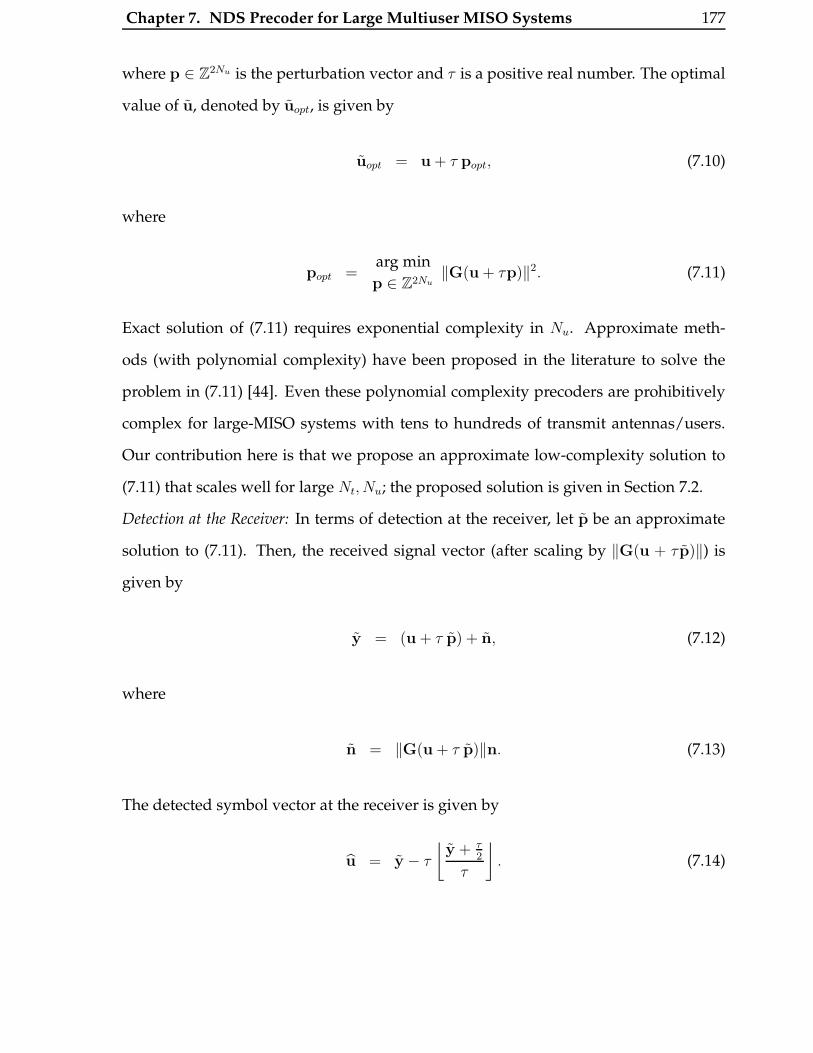
Chapter 7. NDS Precoder for Large Multiuser MISO Systems 177
where p ∈ Z2Nu is the perturbation vector and τ is a positive real number. The optimal
value of u, denoted by uopt, is given by
uopt = u + τ popt, (7.10)
where
popt =arg min
p ∈ Z2Nu‖G(u + τp)‖2. (7.11)
Exact solution of (7.11) requires exponential complexity in Nu. Approximate meth-
ods (with polynomial complexity) have been proposed in the literature to solve the
problem in (7.11) [44]. Even these polynomial complexity precoders are prohibitively
complex for large-MISO systems with tens to hundreds of transmit antennas/users.
Our contribution here is that we propose an approximate low-complexity solution to
(7.11) that scales well for large Nt, Nu; the proposed solution is given in Section 7.2.
Detection at the Receiver: In terms of detection at the receiver, let p be an approximate
solution to (7.11). Then, the received signal vector (after scaling by ‖G(u + τ p)‖) is
given by
y = (u + τ p) + n, (7.12)
where
n = ‖G(u + τ p)‖n. (7.13)
The detected symbol vector at the receiver is given by
u = y − τ
⌊y + τ
2
τ
⌋. (7.14)
Chapter 7. NDS Precoder for Large Multiuser MISO Systems 178
In (7.14), the operation is defined on each entry of the vector since each user gets only
one entry of the vector y. τ is a positive real scalar whose value is fixed. Choice of the
value of τ affects the overall performance. Too high a value is good as far as mitigating
the effect of receiver noise is concerned (since the constellation replicas are placed far
apart, and there is little probability that noise may push a point from one replica to
another), but on the other hand a high value of τ results in a high value of ‖G(u+τ p)‖.
It has been empirically observed that a good choice of τ is given by [32]
τ = 2|cmax|+ δ, (7.15)
where |cmax| is the maximum value of either the real or imaginary component of the
constellation symbols, and δ is the spacing between the constellation symbols. For e.g.,
16-QAM is effectively two 4-PAM constellations in quadrature (taking values of -3, -1,
1, 3 on the real and imaginary axis). Therefore, for 16-QAM, |cmax| is 3, δ is 2, and so τ
is 8. Similarly, for 4-QAM, τ is 4.
7.2 Proposed NDS Precoder
In this section, we present the NDS precoder (see Figure 7.2 for a block diagram), which
is iterative in nature and achieves an approximate solution to the problem in (7.11).
Let u(k) be the perturbed information symbol vector after the kth iteration. We initially
start with u(0) = u, where u is the unperturbed information symbol vector. We perturb
u(k) to get u(k+1) as
u(k+1) = u(k) + τ p(k), (7.16)
where p(k) ∈ Z2Nu is the perturbation vector for the (k + 1)th iteration. To reduce the
computational complexity of the proposed algorithm, we constrain p(k) to have only

Chapter 7. NDS Precoder for Large Multiuser MISO Systems 179
Proposed
NDSAlgorithm
Channel
Proposed NDS Precoder
NormalizedLinear Precoder
(e.g., ZF/MMSE)
eu Hx n yubH
Matrix,GFigure 7.2: Proposed norm-descent search precoder.
one non-zero entry3. Let F4= GTG, where G ∈ R2Nt×2Nu is the precoding matrix.
Further, let q(k) be the power (squared-norm) of the precoded symbol vector after the
kth iteration. Therefore, q(k) is given by
q(k) = ‖Gu(k)‖2 = u(k)T
F u(k). (7.17)
In the (k +1)th iteration, the algorithm finds a constrained integer vector p(k) such that
q(k+1) ≤ q(k). Let
∆q(k+1) 4= q(k+1) − q(k). (7.18)
Let ei denote a 2Nu-dimensional vector with its ith entry only to be one, and all the
other entries to be zero. Since we allow only one non-zero entry in p(k), we can express
p(k) as a scaled integer multiple of some ei, i = 1, · · · , 2Nu. ∆q(k+1) can be negative for
more than one choice of i. The natural question is therefore to select the appropriate
i. Let us denote by ∆q(k+1)i , the value of ∆q(k+1) when p(k) is a scaled integer multiple
of ei. For each i, there exists a scaling integer for ei, λ(k)i , which minimizes ∆q
(k+1)i . Let
this minimum value of ∆q(k+1)i be denoted by ∆q
(k+1)i,opt . We can therefore express ∆q
(k+1)i,opt
3This is similar to the 1-symbol neighborhood definition in the 1-LAS algorithm for large-MIMOdetection in Chapter 2.
Chapter 7. NDS Precoder for Large Multiuser MISO Systems 180
as
∆q(k+1)i,opt = λ
(k)i
2τ 2 Fi,i + 2λ
(k)i τ zi
(k), (7.19)
where Fi,i is the ith diagonal entry of F, zi(k) is the ith entry of the vector
z(k) 4= Fu(k), (7.20)
and
λ(k)i =
arg min
λ ∈ Z∆q
(k+1)i
=arg min
λ ∈ Z‖G(u(k) + λτei)‖2 − ‖Gu(k)‖2
=arg min
λ ∈ Zλ2Fi,i +
2λ
τu(k)T
Fei
=arg min
λ ∈ Zλ2Fi,i +
2λ
τzi
(k). (7.21)
It can be shown that the exact solution to the minimization problem in (7.21) is given
by
λ(k)i = −sgn(zi
(k))
⌊ |zi(k)|
τFi,i
⌉. (7.22)
Though (7.22) gives a closed-form solution to λ(k)i , we have observed in the simulations
that in cases when λ(k)i is large, the algorithm tends to get trapped in some poor local
minima early in the algorithm. In order to alleviate this phenomenon, we constrain the
value of λ(k)i to be within a set S = {−smax,−(smax − 1), · · · , (smax − 1), smax}, which is
a finite subset of Z, and smax denotes the maximum absolute value in S. For e.g., for 4-
QAM, we have found (through simulations) the appropriate set S to be S = {−1, 0, 1}.
If |λ(k)i | > smax, then λ
(k)i is set to 0, and so is ∆q
(k+1)i,opt . If |λ(k)
i | ≤ smax, then ∆q(k+1)i,opt is
computed as per (7.19). We shall refer to this correction in λ(k)i as λ-adjustment. In the
(k + 1)th iteration, we can therefore calculate ∆q(k+1)i,opt for i = 1, · · · , 2Nu. Given these
Chapter 7. NDS Precoder for Large Multiuser MISO Systems 181
values of λ(k)i , i = 1, · · · , 2Nu, we update u(k) as follows:
u(k+1) = u(k) + τ λ(k)j ej , (7.23)
where
j =arg min
i∆q
(k+1)i,opt . (7.24)
The values of λ(k)j used in (7.23) are after the λ-adjustment described above. We also
need to evaluate z(k+1). From (7.20), we can write
z(k+1) − z(k) = F (u(k+1) − u(k)). (7.25)
Using (7.23), we can rewrite (7.25) as
z(k+1) = z(k) + τλ(k)j fj , (7.26)
where fj refers to the jth column of F. Finally, the algorithm terminates after some
iteration n if
min
i∆q
(n+1)i,opt ≥ 0. (7.27)
It is easy to see that the algorithm guarantees a monotonic descent in ‖Gu(k)‖2 with
every iteration until a local minima is reached. Since i) λ(k)i can take values only from
a finite integer valued set S, and ii) ‖Gu(k)‖2 has a global minima for perturbations
with λ(k)i ∈ S, we can see that the NDS algorithm will terminate in a finite number of
iterations. The listing of the NDS algorithm is presented in Table-7.1.
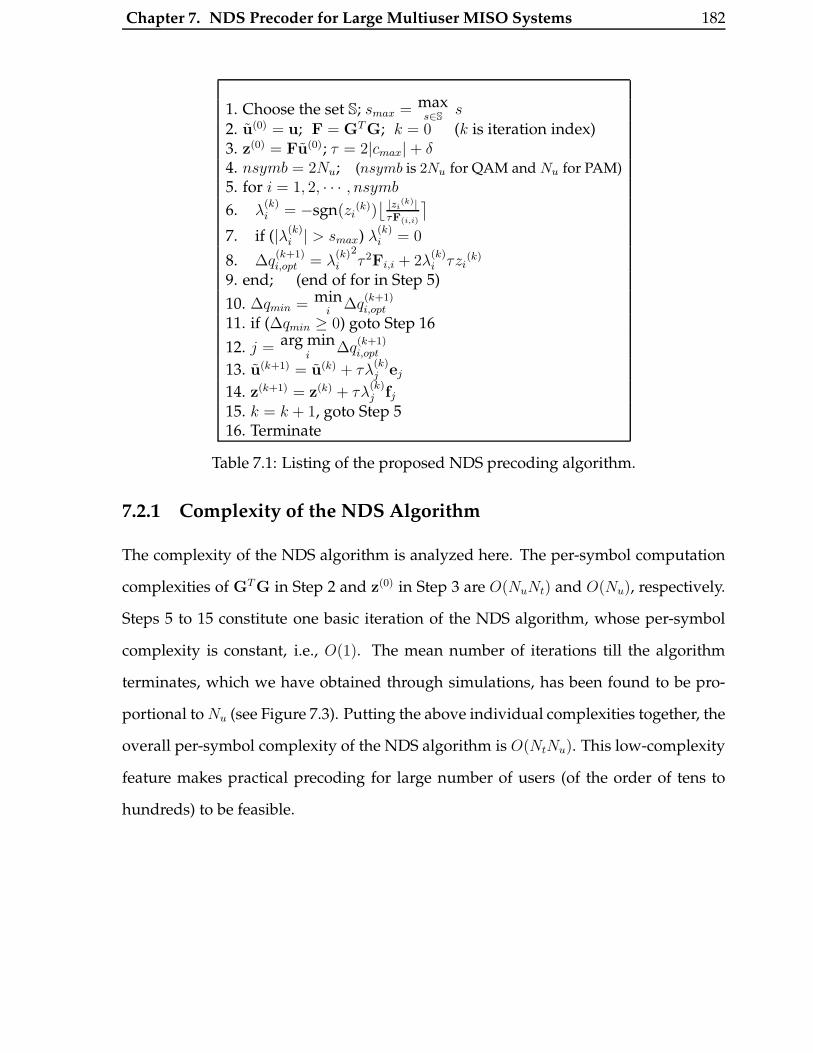
Chapter 7. NDS Precoder for Large Multiuser MISO Systems 182
1. Choose the set S; smax = maxs∈S
s
2. u(0) = u; F = GT G; k = 0 (k is iteration index)3. z(0) = Fu(0); τ = 2|cmax|+ δ4. nsymb = 2Nu; (nsymb is 2Nu for QAM and Nu for PAM)
5. for i = 1, 2, · · · , nsymb
6. λ(k)i = −sgn(zi
(k))⌊ |zi
(k)|τF(i,i)
⌉
7. if (|λ(k)i | > smax) λ
(k)i = 0
8. ∆q(k+1)i,opt = λ
(k)i
2τ 2Fi,i + 2λ
(k)i τzi
(k)
9. end; (end of for in Step 5)
10. ∆qmin = mini
∆q(k+1)i,opt
11. if (∆qmin ≥ 0) goto Step 16
12. j = arg mini
∆q(k+1)i,opt
13. u(k+1) = u(k) + τλ(k)j ej
14. z(k+1) = z(k) + τλ(k)j fj
15. k = k + 1, goto Step 516. Terminate
Table 7.1: Listing of the proposed NDS precoding algorithm.
7.2.1 Complexity of the NDS Algorithm
The complexity of the NDS algorithm is analyzed here. The per-symbol computation
complexities of GTG in Step 2 and z(0) in Step 3 are O(NuNt) and O(Nu), respectively.
Steps 5 to 15 constitute one basic iteration of the NDS algorithm, whose per-symbol
complexity is constant, i.e., O(1). The mean number of iterations till the algorithm
terminates, which we have obtained through simulations, has been found to be pro-
portional to Nu (see Figure 7.3). Putting the above individual complexities together, the
overall per-symbol complexity of the NDS algorithm is O(NtNu). This low-complexity
feature makes practical precoding for large number of users (of the order of tens to
hundreds) to be feasible.
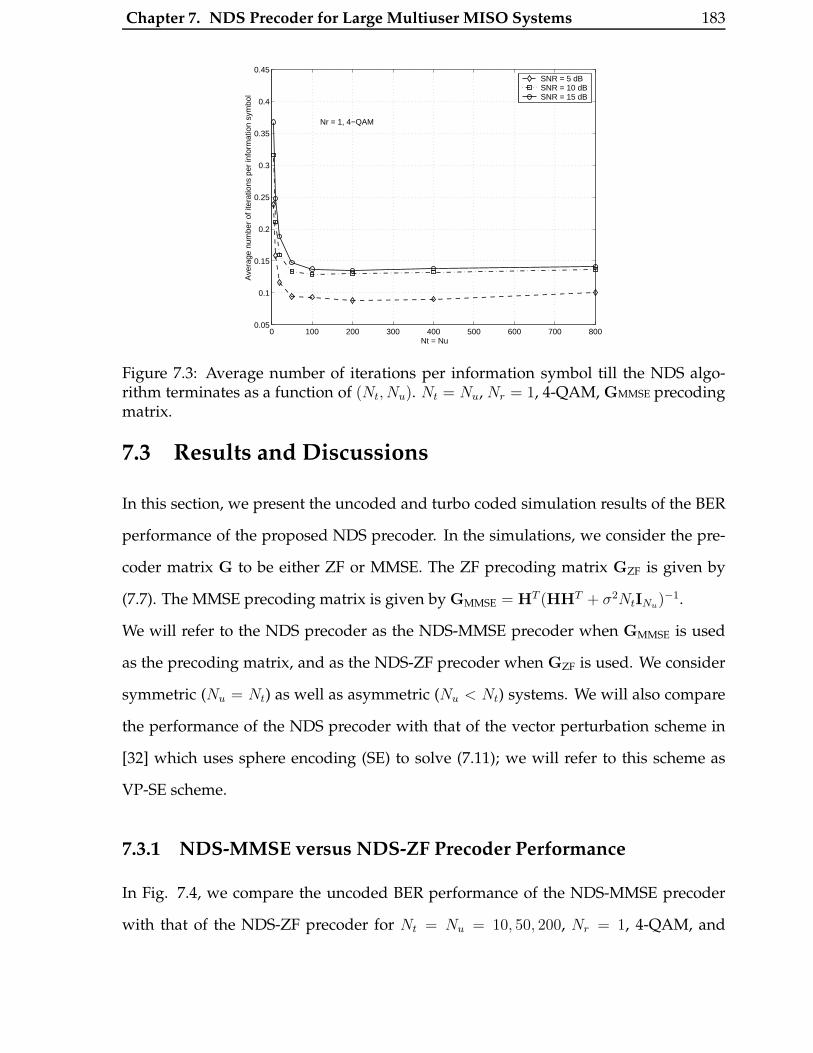
Chapter 7. NDS Precoder for Large Multiuser MISO Systems 183
0 100 200 300 400 500 600 700 8000.05
0.1
0.15
0.2
0.25
0.3
0.35
0.4
0.45
Nt = Nu
Ave
rage
num
ber
of it
erat
ions
per
info
rmat
ion
sym
bol
SNR = 5 dBSNR = 10 dBSNR = 15 dB
Nr = 1, 4−QAM
Figure 7.3: Average number of iterations per information symbol till the NDS algo-rithm terminates as a function of (Nt, Nu). Nt = Nu, Nr = 1, 4-QAM, GMMSE precodingmatrix.
7.3 Results and Discussions
In this section, we present the uncoded and turbo coded simulation results of the BER
performance of the proposed NDS precoder. In the simulations, we consider the pre-
coder matrix G to be either ZF or MMSE. The ZF precoding matrix GZF is given by
(7.7). The MMSE precoding matrix is given by GMMSE = HT (HHT + σ2NtINu)−1.
We will refer to the NDS precoder as the NDS-MMSE precoder when GMMSE is used
as the precoding matrix, and as the NDS-ZF precoder when GZF is used. We consider
symmetric (Nu = Nt) as well as asymmetric (Nu < Nt) systems. We will also compare
the performance of the NDS precoder with that of the vector perturbation scheme in
[32] which uses sphere encoding (SE) to solve (7.11); we will refer to this scheme as
VP-SE scheme.
7.3.1 NDS-MMSE versus NDS-ZF Precoder Performance
In Fig. 7.4, we compare the uncoded BER performance of the NDS-MMSE precoder
with that of the NDS-ZF precoder for Nt = Nu = 10, 50, 200, Nr = 1, 4-QAM, and

Chapter 7. NDS Precoder for Large Multiuser MISO Systems 184
0 5 10 15 20 25 30
10−4
10−3
10−2
10−1
100
Average Received SNR (dB)
Bit
Err
or R
ate
NDS−ZF, N u = 10
NDS−MMSE, N u = 10
NDS−ZF, N u = 50
NDS−MMSE, N u = 50
NDS−ZF, N u = 200
NDS−MMSE,Nu = 200
SISO AWGN
Nt = N
u , N
r = 1
4−QAM
Figure 7.4: Uncoded BER performance of the proposed NDS-MMSE and NDS-ZF pre-coders for Nt = Nu = 10, 50, 200. Nr = 1, 4-QAM.
perfect knowledge of the channel gains. As expected, it is observed that the NDS-
MMSE precoder performs better than the NDS-ZF precoder. For Nt = Nu = 50 and
a target BER of 10−3, NDS-MMSE requires about 5 dB less SNR when compared to
NDS-ZF. Also, NDS-MMSE achieves this better performance at the same complexity
order as that of NDS-ZF, making it more power efficient than NDS-ZF. It can also be
observed that the NDS-MMSE precoder exhibits ’large-system effect,’ where the BER
performance for Nt = Nu = 200 is better than for Nt = Nu = 50. This is similar to
the large-system effect we observed for the LAS and PDA based detection in point-to-
point large-MIMO links presented in Chapters 2 and 3. The fact that it is possible to
get the simulated BER performance of the NDS-MMSE precoder for such large number
of users like 200 users4 illustrates the suitability of the proposed precoder for large
multiuser MISO systems.
4While tens to hundreds of single-antenna downlink users can be envisioned easily in a practicalsystem, base stations with hundreds of antennas may look quite futuristic. However, we point to refer-ence [100], where Thomas Marzetta observes that “...Even in short coherence intervals (say five-hundredmicroseconds) and low SINRs (minus-ten dB reverse, and zero dB forward) a base station comprisingsixteen or more antennas can both learn the forward channel via TDD reciprocity, and transmit, withhigh aggregate throughput, multiple data streams to multiple single-antenna terminals. It is always
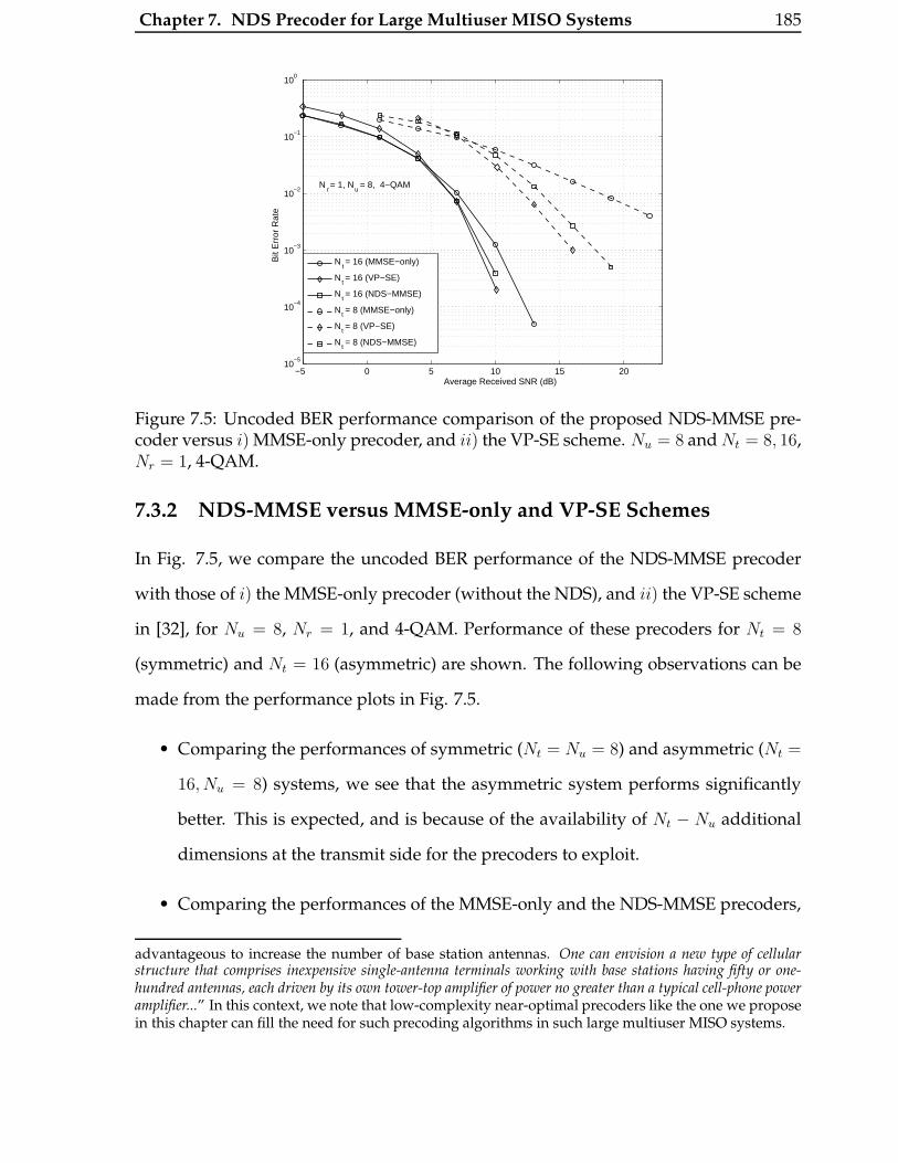
Chapter 7. NDS Precoder for Large Multiuser MISO Systems 185
−5 0 5 10 15 2010
−5
10−4
10−3
10−2
10−1
100
Average Received SNR (dB)
Bit
Err
or R
ate
Nt = 16 (MMSE−only)
Nt = 16 (VP−SE)
Nt = 16 (NDS−MMSE)
Nt = 8 (MMSE−only)
Nt = 8 (VP−SE)
Nt = 8 (NDS−MMSE)
Nr = 1, N
u = 8, 4−QAM
Figure 7.5: Uncoded BER performance comparison of the proposed NDS-MMSE pre-coder versus i) MMSE-only precoder, and ii) the VP-SE scheme. Nu = 8 and Nt = 8, 16,Nr = 1, 4-QAM.
7.3.2 NDS-MMSE versus MMSE-only and VP-SE Schemes
In Fig. 7.5, we compare the uncoded BER performance of the NDS-MMSE precoder
with those of i) the MMSE-only precoder (without the NDS), and ii) the VP-SE scheme
in [32], for Nu = 8, Nr = 1, and 4-QAM. Performance of these precoders for Nt = 8
(symmetric) and Nt = 16 (asymmetric) are shown. The following observations can be
made from the performance plots in Fig. 7.5.
• Comparing the performances of symmetric (Nt = Nu = 8) and asymmetric (Nt =
16, Nu = 8) systems, we see that the asymmetric system performs significantly
better. This is expected, and is because of the availability of Nt − Nu additional
dimensions at the transmit side for the precoders to exploit.
• Comparing the performances of the MMSE-only and the NDS-MMSE precoders,
advantageous to increase the number of base station antennas. One can envision a new type of cellularstructure that comprises inexpensive single-antenna terminals working with base stations having fifty or one-hundred antennas, each driven by its own tower-top amplifier of power no greater than a typical cell-phone poweramplifier...” In this context, we note that low-complexity near-optimal precoders like the one we proposein this chapter can fill the need for such precoding algorithms in such large multiuser MISO systems.

Chapter 7. NDS Precoder for Large Multiuser MISO Systems 186
we see that carrying out the proposed norm-descent search prior to MMSE pre-
coding achieves much better diversity order compared to MMSE-only precoding.
Given that the additional search operation itself is of low-complexity, i.e., O(Nu)
per-symbol complexity, compared to the O(NtNu) per-symbol complexity of the
GTG and MMSE operations, this improvement is quite significant.
• Comparing the performances of the proposed NDS-MMSE scheme and the VP-
SE scheme, we see that the VP-SE scheme performs better at moderate to high
SNRs. However, the NDS-MMSE performance is quite close to that of the VP-
SE scheme at these SNRs. For e.g., for Nt = 16, the SNR gap between VP-SE
and NDS-MMSE performances at 10−3 BER is just about 0.4 dB. The NDS-MMSE
scheme achieves such good performance at a much reduced complexity com-
pared to the exponential complexity of the VP-SE scheme in solving (7.11). Fur-
ther, perturbation based schemes perform relatively poor at low SNRs, since the
optimum choice of the perturbation vector p is made based on minimizing the
average transmit power and not based on minimizing the BER. In fact, the NDS-
MMSE and MMSE-only performances are slightly better than that of the VP-SE
scheme at low SNRs.
Complexity Comparison Between NDS-MMSE and VP-SE Schemes
In Fig. 7.6, we present a complexity comparison between the NDS-MMSE and VP-SE
schemes for Nt = Nu, Nr = 1, 4-QAM at 15 dB SNR. We have plotted the complex-
ity, measured in terms of mean CPU run time (in seconds) needed for precoding an
information symbol vector u into the transmit vector x. Since the complexity is depen-
dent on the channel realization H, we averaged it over a large number of independent
channel realizations. The measured CPU run times in the simulations are shown in the
figure. We see that the search in VP-SE scheme has exponential complexity in Nt, as ev-
idenced by its complexity curve running parallel to the cex2Nu curve for large Nu. This
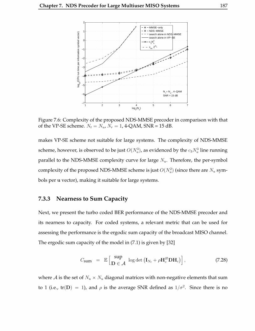
Chapter 7. NDS Precoder for Large Multiuser MISO Systems 187
1 2 3 4 5 6 7−7
−6
−5
−4
−3
−2
−1
0
1
2
log2(N
u)
log 10
(CP
U r
un ti
me
per
info
rmat
ion
sym
bol v
ecto
r)
MMSE−onlyNDS−MMSEsearch alone in NDS−MMSEsearch alone in VP−SE
c3N
u3
cex
2Nu
Nt = N
u , 4−QAM
SNR = 15 dB
Figure 7.6: Complexity of the proposed NDS-MMSE precoder in comparison with thatof the VP-SE scheme. Nt = Nu, Nr = 1, 4-QAM, SNR = 15 dB.
makes VP-SE scheme not suitable for large systems. The complexity of NDS-MMSE
scheme, however, is observed to be just O(N3u), as evidenced by the c3N
3u line running
parallel to the NDS-MMSE complexity curve for large Nu. Therefore, the per-symbol
complexity of the proposed NDS-MMSE scheme is just O(N2u) (since there are Nu sym-
bols per u vector), making it suitable for large systems.
7.3.3 Nearness to Sum Capacity
Next, we present the turbo coded BER performance of the NDS-MMSE precoder and
its nearness to capacity. For coded systems, a relevant metric that can be used for
assessing the performance is the ergodic sum capacity of the broadcast MISO channel.
The ergodic sum capacity of the model in (7.1) is given by [32]
Csum = E
[ sup
D ∈ A log det(INt + ρHH
c DHc
)], (7.28)
where A is the set of Nu × Nu diagonal matrices with non-negative elements that sum
to 1 (i.e., tr(D) = 1), and ρ is the average SNR defined as 1/σ2. Since there is no
Chapter 7. NDS Precoder for Large Multiuser MISO Systems 188
closed-form expression for the optimization in (7.28), we have to evaluate it through
Monte-Carlo simulations. Monte-Carlo simulations are prohibitive for large systems,
and so we consider upper and lower bounds to the sum capacity in the following. We
note that D = DCSIR4= 1
NtINt satisfies the trace constraint, and therefore
CCSIR4= E
[log det
(INt +
ρ
NtHH
c Hc
)](7.29)
is a lower bound for Csum, i.e., Csum ≥ CCSIR. We also note that CCSIR is the ergodic
capacity of a point-to-point single-user MIMO system with Nt receive antennas and Nu
transmit antennas with CSIR only. On the other hand, receiver cooperation between
the users will increase the capacity, and therefore we see that the sum capacity Csum
is upper bounded by the capacity of a point-to-point MIMO system with Nt transmit
antennas and Nu receive antennas with CSIT and CSIR. We shall denote this upper
bound by CCSIT.
In Fig. 7.7, we plot the upper (CCSIT) and lower (CCSIR) bounds to the sum capacity
Csum. It is observed that the gap between the bounds diminishes with increasing SNR,
and therefore any of these bounds is a good approximation at high SNR. However,
at low SNRs, there is a gap between the bounds, which diminishes as the system be-
comes more asymmetrical. For e.g., with Nu = 8 users and a target spectral efficiency
of 1.5 bps/Hz for each user, the gap between the upper and lower bounds is 0.5, 0.8
and 1.3 dB for Nt = 16, 12, and 8, respectively. For small systems, it has been observed
through Monte-Carlo simulations that the ergodic sum capacity is almost same as the
lower bound CCSIR [32]. We will evaluate the nearness of the NDS-MMSE scheme per-
formance with turbo coding w.r.t to the upper bound on Csum.
Turbo Coded BER Performance
Figure 7.8 shows the turbo coded BER performance of the NDS-MMSE and VP-SE
schemes for Nu = 8, Nt = 8, 12, 16, 4-QAM, Nr = 1, and rate-3/4 turbo code. The sum

Chapter 7. NDS Precoder for Large Multiuser MISO Systems 189
−6 −4 −2 0 2 4 6 8 10 120
5
10
15
20
25
30
35
40
Average Received SNR ( dB)
Cap
acity
(bp
s/H
z)
CCSIR
Nt = 8 N
u = 8
CCSIT
Nt = 8 N
u = 8
CCSIR
Nt = 12 N
u = 8
CCSIT
Nt = 12 N
u = 8
CCSIR
Nt = 16 N
u = 8
CCSIT
Nt = 16 N
u = 8
Figure 7.7: Upper and lower bounds for the ergodic sum capacity, Csum.
rate achieved in this system is 8×2×3/4 = 12 bps/Hz. The minimum SNR required to
achieve a sum rate of 12 bps/Hz obtained from the upper bound on the sum capacity
are also shown. From Fig. 7.8, it can be seen that the VP-SE scheme achieves vertical
fall in coded BER at about 9.2, 7.8 and 7.2 dB away from the respective theoretical
minimum SNRs required for Nt = 8, 12 and 16. It is further seen that the vertical fall
for the NDS-MMSE scheme for Nt = Nu = 8 occurs at about 1.5 dB away from that of
the VP-SE scheme. For the asymmetric cases of Nt = 12 and Nt = 16, the performance
of the NDS-MMSE scheme is about 0.5 dB better than that of the VP-SE scheme.
We further note that while VP-SE scheme performance can be evaluated for small sys-
tems as shown in Fig. 7.8, evaluation of its performance for hundreds of users is pro-
hibitively complex. On the other hand, performance in such large systems with the
proposed NDS-MMSE precoder can be evaluated due its low complexity. We highlight
this point in Fig. 7.9, where we have plotted the turbo coded BER performance of the
NDS-MMSE scheme for a large system with Nt = Nu = 300, Nr = 1, 4-QAM, rate-3/4
turbo code, and sum rate = 450 bps/Hz. To illustrate the effect of channel estimation
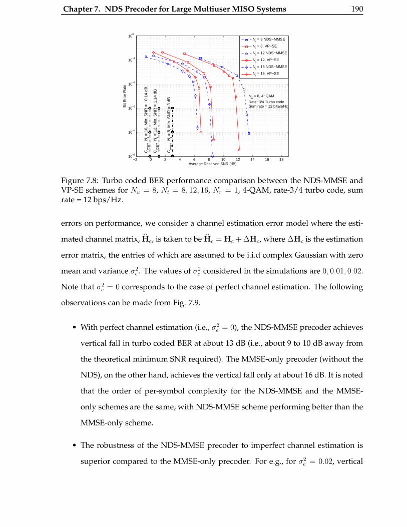
Chapter 7. NDS Precoder for Large Multiuser MISO Systems 190
−2 0 2 4 6 8 10 12 14 16 1810
−5
10−4
10−3
10−2
10−1
100
Average Received SNR (dB)
Bit
Err
or R
ate
CC
SIT
Nt =
16,
Min
. SN
R =
−0.
14 d
B
CC
SIT
Nt =
12,
Min
. SN
R =
1.1
4 dB
CC
SIT
Nt =
8, M
in. S
NR
= 3
dB
Nt = 8 NDS−MMSE
Nt = 8, VP−SE
Nt = 12 NDS−MMSE
Nt = 12, VP−SE
Nt = 16 NDS−MMSE
Nt = 16, VP−SE
Nu = 8, 4−QAM
Rate−3/4 Turbo codeSum rate = 12 bits/s/Hz
Figure 7.8: Turbo coded BER performance comparison between the NDS-MMSE andVP-SE schemes for Nu = 8, Nt = 8, 12, 16, Nr = 1, 4-QAM, rate-3/4 turbo code, sumrate = 12 bps/Hz.
errors on performance, we consider a channel estimation error model where the esti-
mated channel matrix, Hc, is taken to be Hc = Hc + ∆Hc, where ∆Hc is the estimation
error matrix, the entries of which are assumed to be i.i.d complex Gaussian with zero
mean and variance σ2e . The values of σ2
e considered in the simulations are 0, 0.01, 0.02.
Note that σ2e = 0 corresponds to the case of perfect channel estimation. The following
observations can be made from Fig. 7.9.
• With perfect channel estimation (i.e., σ2e = 0), the NDS-MMSE precoder achieves
vertical fall in turbo coded BER at about 13 dB (i.e., about 9 to 10 dB away from
the theoretical minimum SNR required). The MMSE-only precoder (without the
NDS), on the other hand, achieves the vertical fall only at about 16 dB. It is noted
that the order of per-symbol complexity for the NDS-MMSE and the MMSE-
only schemes are the same, with NDS-MMSE scheme performing better than the
MMSE-only scheme.
• The robustness of the NDS-MMSE precoder to imperfect channel estimation is
superior compared to the MMSE-only precoder. For e.g., for σ2e = 0.02, vertical

Chapter 7. NDS Precoder for Large Multiuser MISO Systems 191
0 5 10 15 20 25 3010
−5
10−4
10−3
10−2
10−1
100
Average Received SNR (dB)
Bit
Err
or R
ate
CC
SIR
Min
. SN
R =
4.3
dB
Nt = Nu = 300, Nr =1 Turbo Rate−3/4, 4−QAM
CC
SIT
Min
. SN
R =
3 d
B
Coded NDS−MMSE (Est. Err. Var = 0)Coded NDS−MMSE (Est. Err. Var = 0.02)Coded MMSE−only ((Est. Err. Var = 0)Coded MMSE−ony ((Est. Err. Var = 0.02)Uncoded NDS−MMSE (Est. Err. Var = 0.05)Uncoded NDS−MMSE (Est. Err. Var = 0.02)Uncoded NDS−MMSE (Est. Err. Var = 0.01)Uncoded NDS−MMSE (Est. Err. Var = 0)Uncoded MMSE−only (Est. Err. Var = 0)
Figure 7.9: Turbo coded BER performance of the proposed NDS-MMSE precoder with-out and with channel estimation errors. Nt = Nu = 300, Nr = 1, 4-QAM, rate-3/4 turbocode, sum rate = 450 bps/Hz.
fall occurs at about 15 dB for the NDS-MMSE precoder, whereas for the MMSE-
only precoder vertical fall does not occur and a high error floor results.
We note that search for other low-complexity precoding algorithms for large multiuser
MISO/MIMO systems, like the proposed NDS precoder, can be a topic of further in-
vestigation. Channel estimation issues in large multiuser MISO/MIMO systems can
also be investigated further.

Chapter 8
Conclusions
In this thesis, we investigated low-complexity detection and precoding algorithms that
can potentially enable practical realization of large-MIMO systems with tens of anten-
nas in wireless communication terminals.
In Chapters 2, 3, and 4, we dealt with large-MIMO detection and channel estimation.
Large-MIMO precoding was the subject matter in Chapters 5 and 6. Precoding for
large multiuser MISO systems was investigated in Chapter 7.
In Chapter 2, we presented a low-complexity LAS algorithm suited for detection in
large V-BLAST MIMO and non-orthogonal STBC MIMO systems with tens of anten-
nas that achieve high spectral efficiencies of the order of several tens to hundreds of
bps/Hz. The algorithm was shown to exhibit large-system behavior, where the bit er-
ror performance improved with increasing number of antennas, and approached near-
ML performance for large number of dimensions. We also presented a training-based
iterative detection/channel estimation scheme for large-MIMO systems. Our simula-
tion results showed that the LAS detector along with the iterative detection/channel
estimation scheme achieved very good performance at low complexities. Subsequent
to our reporting of the LAS algorithm for large-MIMO detection in the literature, other
authors have reported FPGA implementation of 32× 32 V-BLAST MIMO detection for
4-/16-/64-QAM using the proposed LAS algorithm.
192
Chapter 8. Conclusions 193
In Chapter 3, we presented a performance analysis of the LAS algorithm in the large-
system limit, where Nt, Nr →∞ with Nt = Nr.
In Chapter 4, we presented another low-complexity algorithm for large-MIMO detec-
tion, which is based on PDA. We showed that the PDA algorithm too exhibited large-
system behavior, which, along with the low-complexity attribute, made the PDA algo-
rithm as another promising algorithm for large-MIMO detection.
We note that with the feasibility of low-complexity high-performance detection algo-
rithms like the proposed LAS and PDA algorithms, in conjunction with the iterative de-
tection/channel estimation scheme, large-MIMO systems with tens of antennas at high
spectral efficiencies can become practical, enabling interesting high data rate wireless
applications (e.g., wireless IPTV/HDTV distribution). This can motivate the inclusion
of large-MIMO architectures (e.g., 12× 12, 16× 16, 24× 24, 32× 32 MIMO systems, in-
cluding those using STBCs from CDA) into wireless standards like IEEE 802.11ac and
IEEE 802.16/LTE-A in their evolution to achieve high data rates (multi-gigabit rates)
at increased spectral efficiencies (in excess of 50 bps/Hz).
In Chapter 5, we proposed X-, Y-Codes/Precoders for large-MIMO precoding which
can achieve full-rate and high diversity at low complexity by pairing the subchan-
nels prior to SVD precoding. It was observed that indeed pairing of channels can
significantly improve the overall diversity. Among all possible pairings, pairing the
kth channel with the (Nr − k + 1)th subchannel was found to be optimal in terms of
achieving the best diversity order. One way of pairing the subchannels is by using
rotation based encoding as for X-Codes/Precoders. The proposed X-Codes/Precoders
have good performance for well conditioned channels. For ill-conditioned channels,
we then proposed Y-Codes/Precoders. It was shown that Y-Codes/Precoders achieve
the best error performance at very low complexity, when compared to other precoders
in the literature. In practice, in order to improve the overall performance, it is possible
to adaptively switch between X- and Y-Codes/Precoders depending on the channel

Chapter 8. Conclusions 194
conditions.
In Chapter 6, we proposed a low-complexity precoding scheme based on the pairing
of subchannels, which achieves near optimal capacity for Gaussian MIMO channels
with discrete inputs. The low-complexity feature relates to both the evaluation of the
optimal precoder matrix and the detection at the receiver. This makes the proposed
scheme suitable for practical applications, even when the channels are time varying
and the precoder needs to be computed for each channel realization. The simple pre-
coder structure, inspired by the X-Codes, enabled us to split the precoder optimization
problem into two simpler problems. Firstly, for a given pairing and power allocation
between pairs, we need to find the optimal power fraction allocation and rotation an-
gle for each pair. Given the solution to the first problem, the second problem is then to
find the optimal pairing and the power allocation between pairs. For large number of
subchannels, typical of OFDM and large-MIMO systems, we also discussed different
heuristic approaches for optimizing the pairing of subchannels. The proposed pre-
coder was shown to perform close to the optimal precoder with discrete inputs, and
significantly better than the Mercury/waterfilling strategy for both diagonal and non-
diagonal MIMO channels. Future work can focus on finding close to optimal pairings,
and close to optimal power allocation strategies between pairs.
In Chapter 7, we presented a low-complexity NDS precoder for large multiuser MISO
systems. The NDS precoder was shown to perform close to the sphere encoder based
vector perturbation scheme, but at a much lower complexity. So, the NDS precoder is
suited, in terms of both complexity as well as performance, for large multiuser MISO
systems with tens to hundreds of downlink users. The presented precoder was also
shown to be robust to channel estimation errors. The feasibility of low-complexity
precoders, like the NDS precoders we presented, can potentially trigger wide interest
in the theory and implementation of large multiuser MISO/MIMO systems.
In concluding this thesis, we point out that the area of low-complexity near-optimal

Chapter 8. Conclusions 195
signal processing for large-MIMO systems is both nascent as well as hugely promising.
We believe that very high spectral efficiency wireless systems employing large number
of antennas will be practical in the near future, and that the work reported in this thesis
can be viewed as a development in that direction.
Appendix A
Proof of Optimum Update l(k)p , Chapter
2
Theorem: The l(k)p in (2.27) minimizes F(l
(k)p ) in (2.25) and this minimum value is non-
positive.
Proof: Let r4=⌊|z(k)
p |2ap
⌋. Then
|z(k)p |
2ap= r + f , where 0 ≤ f < 1, and so we can write
|z(k)p |ap
= 2r + 2f. (A.1)
If l(k)p were unconstrained to be any real number, then the optimal value of l
(k)p is
|z(k)p |ap
,
which would lie between 2r and 2r +2 (as per (A.1)). Since F(l(k)p ) is quadratic in l
(k)p , it
is unimodular, and hence the optimal point (with l(k)p constrained) would be either 2r
or 2r + 2. Using (2.25) and (A.1), we can evaluate F(2r + 2)− F(2r) to be
F(2r + 2)−F(2r) = 4ap(1− 2f). (A.2)
Since ap is a positive quantity, the sign of F(2r + 2)− F(2r) depends upon the sign of
(1 − 2f). If f ≥ 0.5, then F(2r + 2) ≤ F(2r), and therefore 2r + 2 is the optimal value
of l(k)p . Similarly, when f < 0.5, 2r is the optimal value of l
(k)p . Therefore, it follows that
indeed the rounding solution given by (2.27) is optimal. F(l(k)p ) is non-positive for all
196

Appendix A. Proof of Optimum Update l(k)p , Chapter 2 197
values of l(k)p between zero and
2|z(k)p |
ap. If f < 0.5, then 2r is optimal, and, from (A.1), we
know that 2r ≤ |z(k)p |ap
, and therefore 2r < 2|z(k)
p |ap
. Hence F (2r) = F (opt) is non-positive.
Similarly, if f ≥ 0.5, then 2r + 2 is optimal, and F(2r + 2) ≤ F(2r). However, since
2r is always less than 2|z(k)
p |ap
, F(2r) is non-positive and therefore F(2r + 2) = F (opt) is
non-positive.

Appendix B
Proof of Lemma 5, Chapter 3
We present the proof of Lemma 5 of Chapter 3. The proof is by mathematical induction
on n.
Base Case: For n = 2, we have to show that
dp dq
hTp hq
‖hp‖2 + ‖hq‖2p−→ 0 as Nt →∞, ∀ p, q = 1, 2, · · · , 2Nt, p 6= q. (B.1)
We can write the random variablehT
p hq
‖hp‖2+‖hq‖2 as
hTp hq/(2Nt)
(‖hp‖2 + ‖hq‖2)/(2Nt). (B.2)
As Nt → ∞, by strong law of large numbers, the denominator of (B.2) converges to 1
almost surely. Also, the numerator of (B.2) can be written as
hTp hq
2Nt
=
∑2Nt
k=1 hp,khq,k
2Nt
, (B.3)
where hp,k and hq,k refer to the kth entry of the vectors hp and hq , respectively. Each
hp,khq,k term in the summation in (B.3) has the same distribution and has mean 0.
Therefore, by strong law of large numbers, we can see thathT
p hq
2Ntconverges to 0 almost
surely. This also implies thathT
p hq
2Ntconverges in distribution to the constant 0, and hence
198
Appendix B. Proof of Lemma 5, Chapter 3 199
by Slutsky’s theorem,hT
p hq
‖hp‖2+‖hq‖2 converges in distribution to 0. Since, if a sequence of
r.v’s converges in distribution to a constant then the sequence converges in probability
to that constant, we conclude that indeedhT
p hq
‖hp‖2+‖hq‖2 converges in probability to 0. This
proves the the base case.
Induction Hypothesis: Let zun,dp−→ 0 as Nt →∞, ∀n = 2, 3, · · · , m.
Induction Step: Proof for n = m + 1: We have
zu(m+1),d =
∑m+1k=1
∑m+1j=k+1 hT
ijhikdijdik∑m+1
j=1 ‖hij‖2
=
∑mk=1
∑mj=k+1 hT
ijhikdijdik +
∑mk=1 hT
i(m+1)hikdi(m+1)
dik
‖hi(m+1)‖2 +
∑mj=1 ‖hij‖2
=
∑mk=1
∑mj=k+1 hT
ijhik
dijdik∑m
j=1 ‖hij‖2 +
∑mk=1 hT
i(m+1)hik
di(m+1)dik∑m
j=1 ‖hij‖2
1 +‖hi(m+1)
‖2
∑mj=1 ‖hij
‖2
. (B.4)
Using Slutsky’s theorem and the strong law of large numbers, it can be shown that
the denominator in (B.4) converges to (1 + 1m
) in probability. Also, from the induction
hypothesis, the term
∑mk=1
∑mj=k+1 hT
ijhik
dijdik∑m
j=1 ‖hij‖2 in the numerator of (B.4) converges in prob-
ability to 0. Therefore, the numerator in (B.4) converges to the same distribution that
the term
∑mk=1 hT
i(m+1)hik
di(m+1)dik∑m
j=1 ‖hij‖2 converges to. Also, the term
∑mk=1 hT
i(m+1)hik
di(m+1)dik∑m
j=1 ‖hij‖2 is the
same as(∑m
k=1 hTi(m+1)
hikdi(m+1)
dik)/(mNt)
(∑m
j=1 ‖hij‖2)/(mNt)
. Further, from the strong law of large numbers,
the term (∑m
j=1 ‖hij‖2)/(mNt) converges almost surely to 1. Therefore, from Slutsky’s
theorem, we know that(∑m
k=1 hTi(m+1)
hikdi(m+1)
dik)/(mNt)
(∑m
j=1 ‖hij‖2)/(mNt)
converges in distribution to the
distribution to which the term (∑m
k=1 hTi(m+1)
hikdi(m+1)dik)/(mNt) converges.
For a given vector d, hikdik is a random vector whose distribution is the same as that of
hik . Therefore, applying Lemma 4, we see that the term (∑m
k=1 hTi(m+1)
hikdi(m+1)dik)/(mNt)
converges almost surely to 0. Hence, the numerator in (B.4) converges in probability
to the constant 0 . Therefore, zu(m+1),dp−→ 0 as Nt →∞. This proves the induction step
and completes the proof of Lemma 5. �

Appendix C
Conjecture 1, Chapter 3
We present conjecture 1 of Chapter 3 in this appendix. Through the principle of mathe-
matical induction, we conjecture that for any detection algorithmA1(.) satisfying prop-
erty (3.13), and any 0 < δ < 1, for each m = 2, 3, · · ·2Nt, there exists an integer Nm(δ)
such that for all Nt ≥ Nm(δ), and any (x,n), pm(x,n) > (1− δ).
For a given H,x and n, let d4= A1(H,y). We first present the base case for m = 2,
where we show that for a given (x,n), if n ∈ Rd1 , then n ∈ Rd2 with high probability
(w.r.t. the probability distribution of H).
Base Case (m = 2):
Since A1(.) satisfies property (3.13), it must be true that d ∈ D1H,x,n. From (3.12), this
further implies that n ∈ Rd1 . Therefore, from the definition ofRdm , n satisfies (3.6). To
prove the base case we need to consider the event {n ∈ Rd2}.
For n to belong to Rd2 , in addition to satisfying (3.6), n must also satisfy the following
equation ∀ p, q = 1, · · ·2Nt, p 6= q:
(n + H(x− d) + hpdp + hqdq
)T (hpdp + hqdq
)≥ 0, (C.1)
which can be rewritten as
(n + H(x− d)
)Thpdp +
(n + H(x− d)
)Thqdq ≥ −‖hp‖2 − ‖hq‖2 − 2dpdqh
Tp hq. (C.2)
200
Appendix C. Conjecture 1, Chapter 3 201
Since n satisfies (3.6), it satisfies the following two equations:
(n + H(x− d)
)Thpdp ≥ −‖hp‖2,
(n + H(x− d)
)Thqdq ≥ −‖hq‖2. (C.3)
Comparing (C.3) and (C.2), we notice that if hp and hq are orthogonal, then n trivially
satisfies (C.2) for all Nt. Therefore, when hp and hq are non-orthogonal, the only extra
term in the RHS of (C.2) is 2dpdqhTp hq . Applying Lemma 5 of Chapter 3, with n = 2, we
see that as Nt → ∞, the r.v.hT
p hq
‖hp‖2+‖hq‖2 converges to zero in probability. Then, we can
write, for any ε, 0 ≤ ε ≤ 1
p
(|hT
p hq|‖hp‖2 + ‖hq‖2
> ε
)< ε, ∀Nt > f(ε). (C.4)
For each pair (p, q) and a given H we define the following events
E1(p, q,H)4= { |hT
p hq|‖hp‖2 + ‖hq‖2
< ε}
E2(p, q,H)4= { |hT
p hq|‖hp‖2 + ‖hq‖2
> ε}
E3(p, q,H)4= {(n + H(x− d) + hpdp + hqdq
)T (hpdp + hqdq)} < 0
E11(p, q,H)4=
{0 < hT
p hq < ε(‖hp‖2 + ‖hq‖2
)}
E12(p, q,H)4=
{0 > hT
p hq > −ε(‖hp‖2 + ‖hq‖2
)}
E+1(p, q,H)4= {dpdq = +1}
E−1(p, q,H)4= {dpdq = −1}
Ec(p, q,H)4=
(E+1(p, q,H) ∩ E11(p, q,H)
)∪(E−1(p, q,H) ∩E12(p, q,H)
).(C.5)
For n /∈ Rd2 , E3(p, q,H) must be true for at least some pair (p, q). Further, let E3(H)4=
Appendix C. Conjecture 1, Chapter 3 202
∪(p,q) p 6=qE3(p, q,H). p2(x,n) can now be expressed as
p2(x,n) = EH[I(n /∈ Rd2 |H,x,n,d = A1(H,y))]
= EH[I(E3(H) |H,x,n,d = A1(H,y))]
≤∑
(p,q)p 6=q
EH[I(E3(p, q,H) |H,x,n,d = A1(H,y))]. (C.6)
The last inequality follows from the union bound. However, this bound is not very
tight. Due to analytical intractability, it is difficult to get a meaningful bound. This is
the primary difficulty in proving the conjecture. To gain some insight as to why the
conjecture may actually be true, we attempt to bound EH[I(E3(p, q,H) |H,x,n,d =
A1(H,y))] for each (p, q).
EH[I(E3(p, q,H) |H,x,n,d = A1(H,y))]
= EH[I(E3(p, q,H), E1(p, q,H) |H,x,n,d = A1(H,y))]
+ EH[I(E3(p, q,H), E2(p, q,H) |H,x,n,d = A1(H,y))]
< EH[I(E3(p, q,H), E1(p, q,H) |H,x,n,d = A1(H,y))]
+ EH[I(E2(p, q,H) |H,x,n,d = A1(H,y))]
< EH[I(E3(p, q,H), E1(p, q,H) |H,x,n,d = A1(H,y))] + ε
(C.7)
The last inequality follows from (C.4). EH[I(E3(p, q,H), E1(p, q,H) |H,x,n,d = A1(H,y))]
can now be expressed as
EH[I(E3(p, q,H), E1(p, q,H) |H,x,n,d = A1(H,y))]
= EH[I(E3(p, q,H), E1(p, q,H), Ec(p, q,H) |H,x,n,d = A1(H,y))]
+ EH[I(E3(p, q,H), E1(p, q,H), Ec(p, q,H) |H,x,n,d = A1(H,y))], (C.8)
where Ec(p, q,H) denotes the complementary event of Ec(p, q,H).
Appendix C. Conjecture 1, Chapter 3 203
We now make the following important observations. For any pair (p, q), if Ec(p, q,H)
and E1(p, q,H) is true, then
−(‖hp‖2 + ‖hq‖2
)> −
(‖hp‖2 + ‖hq‖2 + 2dpdqh
Tp hq
)> −
(‖hp‖2 + ‖hq‖2
)(1 + 2ε) .
(C.9)
Since n ∈ Rd1 , n satisfies (C.3), and hence satisfies the following equation:
(n + H(x− d))T (hpdp + hqdq) ≥ −(‖hp‖2 + ‖hq‖2
). (C.10)
Using (C.9) and (C.10), we see that n satisfies (C.2). So, if Ec(p, q,H) and E1(p, q,H) are
true, it can be concluded that E3(p, q,H) is false. Therefore,
EH[I(E3(p, q,H), E1(p, q,H), Ec(p, q,H) |H,x,n,d = A1(H,y))] = 0. Hence, this im-
plies that
EH[I(E3(p, q,H), E1(p, q,H) |H,x,n,d = A1(H,y))]
= EH[I(E3(p, q,H), E1(p, q,H), Ec(p, q,H) |H,x,n,d = A1(H,y))]. (C.11)
We next analyze EH[I(E3(p, q,H), E1(p, q,H), Ec(p, q,H) |H,x,n,d = A1(H,y))]. It can
be shown that if the composite event {E3(p, q,H), E1(p, q,H), Ec(p, q,H)} is true, it im-
plies that the following equations are satisfied.
−(‖hp‖2 + ‖hq‖2
)(1− 2ε) > −
(‖hp‖2 + ‖hq‖2 + 2dpdqh
Tp hq
)> −
(‖hp‖2 + ‖hq‖2
)
(n + H(x− d)
)Thpdp +
(n + H(x− d)
)Thqdq ≤ −‖hp‖2 − ‖hq‖2 − 2dpdqh
Tp hq.
(C.12)
Combining the two sub equations in (C.12), we have
(n + H(x− d)
)Thpdp +
(n + H(x− d)
)Thqdq ≤ −
(‖hp‖2 + ‖hq‖2
)(1− 2ε). (C.13)
Appendix C. Conjecture 1, Chapter 3 204
Also, since d ∈ D1x,n,H, we can rewrite (C.13) as
−(‖hp‖2 + ‖hq‖2) ≤ (n + H(x− d))T (hpdp + hqdq) ≤ −(‖hp‖2 + ‖hq‖2)(1− 2ε).
(C.14)
So, it can be stated that if the composite event {E3(p, q,H), E1(p, q,H), Ec(p, q,H)} is
true, it implies (C.14). Let us define the event E4(p, q,H)4={− (‖hp‖2 + ‖hq‖2) ≤
(n + H(x− d))T (hpdp + hqdq) ≤ −(‖hp‖2 + ‖hq‖2)(1− 2ε)}
.
Therefore, I(E3(p, q,H), E1(p, q,H), Ec(p, q,H) |H,x,n,d = A1(H,y))) = 1 implies
that I(E4(p, q,H) |H,x,n,d = A1(H,y))) = 1. Hence,
EH[I(E3(p, q,H), E1(p, q,H), Ec(p, q,H) |H,x,n,d = A1(H,y)))]
< EH[I(E4(p, q,H) |H,x,n,d = A1(H,y)))]. (C.15)
We next define a function f2(ε), ε > 0, as
f2(ε)4= EH[I(E4(p, q,H |H,x,n,d = A1(H,y)))]. (C.16)
Further,
limε→0
f2(ε) = 0, (C.17)
since for each (p, q), as ε → 0, the upper bound on (n + H(x − d))T (hpdp + hqdq) in
(C.14) approaches the lower bound. Similarly, it can also be shown that, f2(ε) is a
monotonically increasing function of ε. Using (C.16), (C.15) can be written as
EH[I(E3(p, q,H), E1(p, q,H), Ec(p, q,H) |H,x,n,d = A1(H,y)))] < f2(ε). (C.18)
Appendix C. Conjecture 1, Chapter 3 205
Using (C.11) and (C.18), (C.7) can be written as
EH[I(E3(p, q,H) |H,x,n,d = A1(H,y)))] < f2(ε) + ε. (C.19)
Now, define g2(ε)4= f2(ε) + ε. g2 is a monotonic function and therefore has an inverse
g−12 . Hence, for any δ > 0, there exists an ε such that ε = g−1
2 (δ). Using (C.4) and the
above definitions, we can write that
Nt > f(ε)
> f(g−12 (δ)
)
> N2(δ), (C.20)
where N24= f ◦ g−1
2 . Using (C.19), and the above definitions we can state that
EH[I(E3(p, q,H) |H,x,n,d = A1(H,y)))] > 1− δ. (C.21)
Hence, we have shown that for any δ, 0 ≤ δ ≤ 1, there exists an integer N2(δ) such that
for Nt > N2(δ), any arbitrary pair (p, q) satisfies (C.2) with a high probability of (1− δ).
For n ∈ Rd2 , (C.2) should be satisfied for all possible pairs (p, q). Since we have shown
that indeed (C.2) is satisfied by any arbitrary pair with high probability, we conjecture
that (C.2) would be satisfied by all pairs with high probability.
Induction Hypothesis: For any detection algorithm satisfying property (3.13), and any
0 < δ < 1, there exists an integer Nm−1(δ) such that for all Nt ≥ Nm−1(δ), and any
(x,n), pm−1(x,n) > (1 − δ). In the induction hypothesis, we basically assume that if
n ∈ Rd1 , then n ∈ Rdm−1 with high probability.
Induction Step: We conjecture that for any 0 < δ < 1, there exists an integer Nm(δ) such
that for all Nt ≥ Nm(δ), and any (x,n), pm(x,n) > (1 − δ). Based on the definition of
pm(x,n), we conjecture that n ∈ Rdm with high probability. For n to belong to Rdm , n
Appendix C. Conjecture 1, Chapter 3 206
must satisfy the following equation for all possible m-tuples (i1, i2, · · · , im):
(n + H(x− d) +
( m∑
j=1
hijdij
))T( m∑
j=1
hijdij
)≥ 0, (C.22)
which can be written as
(n + H(x− d)
)T(m−1∑
j=1
hijdij
)+(n + H(x− d)
)Thimdim
≥ −‖∑m−1j=1 hijdij‖2 − ‖him‖2 − 2
(∑m−1j=1 hijdij
)T
himdim .(C.23)
However, we know from the induction hypothesis that (n+H(x−d))T (∑m−1
j=1 hijdij) ≥
−‖∑m−1j=1 hijdij‖2 with high probability. Also, since n ∈ Rd1 , we know that (n + H(x−
d))T himdim ≥ −‖him‖2. Therefore, if the term 2(∑m−1
j=1 hijdij)Thimdim in the RHS of
(C.23) were 0, then (C.22) would have been trivially satisfied with high probability. We
now show that the contribution of the term 2(∑m−1
j=1 hijdij )Thimdim when compared to
the other two terms in the RHS (C.23) converges to 0 as Nt →∞.
Define a r.v. vm4=
2(∑m−1
j=1 hijdij
)T himdim
‖∑m−1j=1 hij
dij‖2+‖him‖2
. Our objective is to show that as Nt →∞, vm →
0 in probability. This is equivalent to proving that wm4= vm + 1 =
‖∑m
j=1 hijdij
‖2
‖him‖2+‖∑m−1j=1 hij
dij‖2
converges to one in probability as Nt →∞. We can write wm as
wm =
‖∑m
j=1 hijdij
‖2
∑mj=1 ‖hij
‖2
‖him‖2∑m
j=1 ‖hij‖2 +
‖(∑m−1j=1 hij
dij)‖2
∑mj=1 ‖hij
‖2
. (C.24)
From Lemma 5 of Chapter 3, we know that for any integer m, 1 ≤ m ≤ 2Nt, it is
true that
∑mk=1
∑mj=k+1 hT
ijhik
dijdik∑m
j=1 ‖hij‖2 converges to 0 in probability as Nt → ∞. By Slutsky’s
theorem, this is equivalent to
2∑m
k=1
∑mj=k+1 hT
ijhikdijdik∑m
j=1 ‖hij‖2+ 1 =
‖∑j=mj=1 hijdij‖2∑mj=1 ‖hij‖2
p−→ 1 (C.25)
as Nt → ∞. We shall use this result to prove the convergence of wm in (C.24). Using
Appendix C. Conjecture 1, Chapter 3 207
(C.25), it can be seen that the numerator of wm in (C.24) converges to 1 as Nt →∞, i.e.,
‖∑mj=1 hijdij‖2∑mj=1 ‖hij‖2
p−→ 1, as Nt →∞. (C.26)
In the denominator of (C.24), it can be shown that the term
‖him‖2∑mj=1 ‖hij‖2
p−→ 1
m, as Nt →∞. (C.27)
The 2nd term in the denominator of (C.24) can be rewritten as
‖(∑m−1j=1 hijdij)‖2∑mj=1 ‖hij‖2
=
‖(∑m−1
j=1 hijdij
)‖2
∑m−1j=1 ‖hij
‖2
‖him‖2∑m−1
j=1 ‖hij‖2 + 1
. (C.28)
Similar to the derivation of (C.25), we can claim that the numerator in (C.28) converges
to one in probability. From Slutsky’s theorem, it can be shown that ‖him‖2
∑m−1j=1 ‖hij
‖2 con-
verges to 1m−1
in probability. Using this and Slutsky’s theorem, it can be shown that
(C.28) converges to m−1m
in probability. Using this result along with (C.26),(C.27) and
Slutsky’s theorem in (C.24), it can be shown that wm converges to one in probability as
Nt → ∞. This, therefore, implies that vm converges to zero in probability. Following
along the same lines as the conjecture for the base case, it can be conjectured that for
any δ, 0 ≤ δ ≤ 1, there exists an integer Nm(δ) such that for Nt > Nm(δ), pm(x,n) > 1−δ
(i.e. n ∈ Rdm with high probability). This completes the induction step. �
Appendix D
Proof of Theorem 1, Chapter 5
Towards proving Theorem 1, we shall find the following Lemma useful (see Proposi-
tion 1 in [101] for the same lemma and its proof).
Lemma 1. Given a real scalar channel modeled by y =√
αx + n, where x = ±√Es, n ∼
N (0, σ2). Let F (α) = Cαk + o(αk), for α → 0+ be the cdf (cumulative density function)
of α, where C is a constant and k is a positive integer1. Let γ = Es/σ2 be the SNR. Then
the probability of error is given by P (γ) = Eα[Q(√
αγ)]. The asymptotic error probability for
γ →∞ is given by
P =C((2k − 1) · (2k − 3) · · ·5 · 3 · 1)
2γ−k + o(γ−k). (D.1)
�
The proof of Theorem 1 is as follows. Let {<(uk) → <(vk)} denote the pairwise error
event that, given uk was transmitted on the kth pair, the real part of the ML detector
for the kth pair decodes in favor of some other vector <(vk). Further, let us denote the
probability of this event (i.e., PEP) by P′
k(<(uk) → <(vk)). Using the union bounding
technique, P′
k(<(uk)) is then upper bounded by the sum of all the possible pairwise
error probabilities. From (5.22), it is clear that this upper bound on P′
k(<(uk)) induces
1Any function f(x) in a single variable x is said to be o(g(x)), i.e., f(x) = o(g(x)), if f(x)g(x) → 0 as x→ 0.
208
Appendix D. Proof of Theorem 1, Chapter 5 209
an upper bound on P′
k, which is given by
P′
k ≤1
|Sk|∑
<(uk)
∑
<(vk)6=<(uk)
P′
k(<(uk)→ <(vk)). (D.2)
Due to Gaussian noise, this can be further written as
P′
k ≤1
|Sk|∑
<(uk)
∑
<(vk)6=<(uk)
E
[Q(√
d2k(<(uk),<(vk),Ak)
2N0
)], (D.3)
where d2k(<(uk),<(vk),Ak)
4= ‖Mk(<(uk) − <(vk))‖2, and Q(x)
4=∫∞
x1√2π
e−t2/2dt. The
expectation in (D.3) is over the joint distribution of the channel gain (λik , λjk). The
joint pdf (probability density function) of the ordered eigenvalues of H†H, i.e., {λ21 >
λ22 · · · > λ2
Nr} is given by the well known Wishart distribution [104]. However, in (D.3)
evaluating the expectation over (λik , λjk) is still a difficult problem except for trivial
cases (like Nt = Nr = 2). We, therefore, try to bound d2k(<(uk),<(vk),Ak) such that the
bound depends only on λik . Since λik ≥ λjk≥ 0, using the definition of M and Mk we
have
d2k(<(uk),<(vk),Ak) ≥ λ2
ikd2
k(<(uk),<(vk),Ak), (D.4)
where d2k(<(uk),<(vk),Ak)
4= e2
k,1, ek4= Ak(<(uk)−<(vk)). ek,1 denotes the first compo-
nent of the 2-dimensional vector ek. We further define the generalized minimum distance
as follows:
gk(Ak) = min<(uk)6=<(vk)
d2k(<(uk),<(vk),Ak). (D.5)
Since Q(.) is a monotonically decreasing function with increasing argument, we can

Appendix D. Proof of Theorem 1, Chapter 5 210
further upper bound (D.3) using (D.5) as follows:
P′
k ≤ (|Sk| − 1)E
Q
√
λ2ikgk(Ak)
2N0
. (D.6)
For a Rayleigh faded channel, the marginal pdf of the sth eigenvalue λ2s (for λ2
s → 0) is
given by [105]
f(λ2s) = C(s)(λ2
s)Nt(s)Nr(s)−1 + o
((λ2
s)Nt(s)Nr(s)−1
), (D.7)
where Nt(s)4= (Nt − s + 1), Nr(s)
4= (Nr − s + 1) and C(s) is a constant given in [105].
Using the pdf in (D.7), the cdf Fs(u) = P (λ2s ≤ u) (for u→ 0+) is given by
Fs(u) = D(s)uNt(s)Nr(s) + o(uNt(s)Nr(s)
), (D.8)
where D(s)4= C(s)
Nt(s)Nr(s). Using Lemma 1 and (D.8), the bound in (D.6) can be further
written as
P′
k ≤ (|Sk| − 1)ck
(γgk(Ak)
2PT
)−δk
+ o(γ−δk) (D.9)
where δk4= (Nt − ik + 1)(Nr − ik + 1) and ck
4= C(ik)((2 δk−1) . ··· 5 . 3 . 1)
2 δk. �

Appendix E
Proof of Theorem 2, Chapter 5
Let d(θk, λik , λjk)
4= min(p,q)∈S2 d2
k(p, q, θk), where d2k(p, q, θk) is defined in (5.50). The
objective is to find the optimal θk which maximizes d(θk, λik , λjk). The set S2 contains
exactly 8 elements. Also, due to sign symmetry of this set(i.e., if (p, q) ∈ S2, then so do
(p,−q), (−p, q) and (−p,−q)), there are actually only 4 distances to be computed. For a
given angle θk, these distances are enumerated as follows:
d1 = λ2ik
cos2(θk) + λ2jk
sin2(θk) (E.1)
d2 = λ2ik
sin2(θk) + λ2jk
cos2(θk) (E.2)
d3 = λ2ik
(cos(θk) + sin(θk))2 + λ2
jk(cos(θk)− sin(θk))
2 (E.3)
d4 = λ2ik
(cos(θk)− sin(θk))2 + λ2
jk(cos(θk) + sin(θk))
2. (E.4)
Therefore, d(θk, λik , λjk) can be expressed in terms of these distances as
d(θk, λik , λjk) = min(d1, d2, d3, d4)
= min(min(d1, d2), min(d3, d4)). (E.5)
It can be shown that for the maximization in (5.49), it suffices to only consider the range
of θk to be [0, π/4]. Also, it is given that λik ≥ λjkdue to the order of the singular values
in the SVD decomposition and the way in which pairing is done for X-Codes. Using
211

Appendix E. Proof of Theorem 2, Chapter 5 212
these two facts, it can be concluded that
d2 = min(d1, d2) (E.6)
d4 = min(d3, d4), (E.7)
and therefore
d(θk, λik , λjk) = min(d2, d4). (E.8)
Let
βk4=
λik
λjk
. (E.9)
Then, d4 is the minimum iff the following condition is satisfied:
1
β2k
≤ h(θk), (E.10)
where
h(θk)4= 1− 1
sin(2θk) + sin2(θk). (E.11)
It can be seen that over the interval (0 π4], h(θk) is a continuous and monotonically
increasing function. This is because the first derivative w.r.t θk exists and is always
positive. The maximum value of h(θk) over this interval is 13. Therefore, we now con-
sider two situations depending upon whether βk is greater than or less than√
3.
If βk ≤√
3, then 1β2
k
≥ 13. Since h(θk) is always less than 1
3, we can conclude that the
condition in (E.10) is never satisfied, and therefore d2 is the minima. Further, since
λik ≥ λjk, d2 is a monotonically increasing function of θk, and therefore the solution to
the maximization problem in (5.49) is π4.
If βk ≥√
3, then 1β2
k
≤ 13. Since h(θk) is a monotonically increasing function, we observe

Appendix E. Proof of Theorem 2, Chapter 5 213
that d4 is the minima when θk ≥ θ?k; else d2 is the minima. Here, θ?
k is such that θ?k ∈ [0 π
4]
and h(θ?k) = 1
β2k
. Further, it is observed that d2 is a monotonically increasing function of
θk, whereas d4 is monotonically decreasing. Also, d2 = d4 when θk = θ?k. Therefore, it
can be concluded that min(d2, d4) is maximized when θk = θ?k. Hence, for βk ≥
√3, the
solution to the maximization problem in (5.49) is θ?k. We now solve for θ?
k. Using the
definition of h(θk), we have
1
β2k
= 1− 1
sin(2θ?k) + sin2(θ?
k), (E.12)
or equivalently
tan2(θ?k)− 2(β2
k − 1) tan(θ?k) + β2
k = 0. (E.13)
The last equation is quadratic in tan(θ?k), and the solution which results in θ?
k ∈ [0 π4] is
given by
θ?k = tan−1
[(β2
k − 1)−√
((β2k − 1)2 − β2
k)]. (E.14)
Combining the optimal angles obtained for βk ≤√
3 and βk >√
3, we get the solution
to the maximization problem as stated in (5.51). �

Appendix F
Proof of Theorem 3, Chapter 5
We first get an expression for d2k,min(ak, bk) as defined in (5.74). For any code vector at
index v which is even, the nearest distance to any other code vector with even index is
4λ2ika2
k. The nearest distance to any code vector at odd index is λ2ik
a2k +4λ2
jkb2k. The same
holds true if v is odd. Hence, d2k,min(ak, bk) is given by
d2k,min(ak, bk) = min
(4λ2
ika2
k, λ2ika2
k + 4λ2jk
b2k
). (F.1)
Therefore, our objective is to solve the following constrained min-max optimization
problem:
(a?k, b
?k) = arg max
{(ak ,bk)∈R2+|b2k+a2
kM2−1
12=
PTNr
}min
(4λ2
ika2
k, λ2ika2
k + 4λ2jk
b2k
). (F.2)
The first argument of the min(., .) function, T14= 4λ2
ika2
k is geometrically a straight line
w.r.t a2k passing through the origin and attaining a maximum value of
48PT λ2ik
Nr(M2−1)at a2
k =
12PT
Nr(M2−1)(due to the transmit power constraint a2
k ≤ 12PT
Nr(M2−1)). The second argument of
the min(., .) function is T24= (λ2
ika2
k + 4λ2jk
b2k). Since b2
k + a2k
(M2−1)12
= pT
Nr, we can express
T2 as
T2 = λ2jk
(4PT
Nr+ a2
k
(β2
k −M2 − 1
3
)). (F.3)
214

Appendix F. Proof of Theorem 3, Chapter 5 215
From (F.3) we observe that, if β2k ≥ M2−1
3, then T2 is a straight line with positive
slope, with a value of 4λ2jk
PT
Nrat ak = 0 and attaining a maximum value of
12PT λ2ik
Nr(M2−1)
at a2k = 12PT
Nr(M2−1). This maximum value is less than the maximum attained by T1. Since
both T1 and T2 have positive slopes, the minimum among T1 and T2 is maximized at
a?2
k = 12PT
Nr(M2−1), which implies that b?
k = 0. The value of d2k,min(ak, bk) at ak = a?
k is
the maximum value attained by T2. Therefore, when the channel condition exceeds a
certain threshold, it is optimal to allocate all power to the stronger channel only.
On the other hand, if β2k < M2−1
3, then T2 is a straight line with negative slope, whereas
T1 has positive slope, and therefore the minimum between them is maximized when
they are both equal. Therefore, the optimal (a?k, b
?k) must satisfy
4λ2ika?2
k = λ2ika?2
k + 4λ2jk
b?2
k . (F.4)
Using the fact that b?2
k + a?2
kM2−1
12= PT
Nr, the optimal (a?
k, b?k) is given by
(a?k, b
?k) =
√4PT
3Nr√β2
k + M2−19
,
√PT
Nr
βk√β2
k + M2−19
. (F.5)
Using (F.5), the optimal value of d2k,min(ak, bk) for β2
k < M2−13
is given by
d2k,min(a
?k, b
?k) =
16PTλ2ik
Nr
(3β2
k + (M2−1)3
) . (F.6)
�
List of Publications from this Thesis
Journal Papers
1. Saif K. Mohammed, Ahmed Zaki, A. Chockalingam, and B. Sundar Rajan, “High-
rate space-time coded large-MIMO systems: Low-complexity detection and chan-
nel estimation,” IEEE Journal on Selected Topics in Signal Processing (JSTSP): Special
Issue on Managing Complexity in Multiuser MIMO Systems, vol. 3, no. 6, pp. 958-
974, December 2009.
2. K. Vishnu Vardhan, Saif K. Mohammed, A. Chockalingam, and B. Sundar Rajan,
“A low-complexity detector for large MIMO systems and multicarrier CDMA
systems,” IEEE Journal on Selected Areas in Communication (JSAC): Special Issue on
Multiuser Detection for Advanced Communication Systems and Networks, vol. 26,
no.3, pp. 473-485, April 2008.
3. Saif K. Mohammed, E. Viterbo, Y. Hong, and A. Chockalingam, “MIMO precod-
ing with X- and Y-Codes,” submitted to IEEE Transactions on Information theory,
November 2009. Available Online arXiv:0912.1909v1 [cs.IT] 10 Dec 2009.
4. Saif K. Mohammed, E. Viterbo, Y. Hong, and A. Chockalingam, “Precoding by
pairing subchannels to increase MIMO capacity with discrete input alphabets,”
submitted to IEEE Transactions on Information theory, February 2010. Available
Online: arXiv:1002.4263v1 [cs.IT] 23 Feb 2010.
5. Saif K. Mohammed, A. Chockalingam, and B. Sundar Rajan, “Low-complexity
216
List of Publications from this Thesis 217
near-MAP decoding of large non-orthogonal STBCs using PDA,” journal paper
under preparation.
Conference Papers
1. Saif K. Mohammed, E. Viterbo, Y. Hong, and A. Chockalingam, “X-Codes: A
low-complexity full-rate high-diversity achieving precoder for TDD MIMO sys-
tems,” accepted in IEEE International Conference on Communications (ICC’2010),
Cape Town, South Africa, May 2010.
2. Saif K. Mohammed, E. Viterbo, Y. Hong, and A. Chockalingam, “X-Codes,” In-
ternational Zurich Seminar on Communications (IZS’2010), Zurich, Switzerland,
March 2010.
3. Saif K. Mohammed, A. Chockalingam, and B. Sundar Rajan, “Low-complexity
near-MAP decoding of large non-orthogonal STBCs using PDA,” Proc. IEEE In-
ternational Symposium on Information Theory (ISIT’2009), Seoul, Korea, June-July
2009.
4. Ahmed Zaki, Saif K. Mohammed, A. Chockalingam, and B. Sundar Rajan, “A
training-based iterative detection/channel estimation scheme for large non-orth-
ogonal STBC MIMO systems,” Proc. IEEE International Conference on Communica-
tions (ICC’2009), Dresden, Germany, June 2009.
5. Saif K. Mohammed, A. Chockalingam and B. Sundar Rajan, “High-rate space-
time coded large MIMO systems: Low-complexity detection and performance,”
Proc. IEEE Global Communications Conference (GLOBECOM’2008), New Orleans,
USA, December 2008.
6. Saif K. Mohammed, A. Chockalingam, and B. Sundar Rajan, “Low-complexity
detection and performance in multi-gigabit high spectral efficiency large MIMO

List of Publications from this Thesis 218
systems,” Proc. IEEE Personal, Indoor and Mobile Radio Communications Symposium
(PIMRC’2008), Cannes, France, September 2008.
7. Saif K. Mohammed, A. Chockalingam, and B. Sundar Rajan, “A low-complexity
near-ML performance achieving algorithm for large MIMO detection,” Proc. IEEE
International Symposium on Information Theory (ISIT’2008), Toronto, Canada, July
2008.
8. Saif K. Mohammed, K. Vishnu Vardhan, A. Chockalingam, and B. Sundar Rajan,
“Large MIMO systems: A low-complexity detector at high spectral efficiencies,”
Proc. IEEE International Conference on Communications (ICC’2008), Beijing, China,
May 2008.
9. Saif K. Mohammed, A. Chockalingam, and B. Sundar Rajan, “A low-complexity
precoder for large multiuser MISO systems,” Proc. IEEE Vehicular Technology Con-
ference (VTC’2008), Singapore, May 2008.
10. Saif K. Mohammed, E. Viterbo, Y. Hong, and A. Chockalingam, “X- and Y-Codes
for MIMO precoding”, submitted to IEEE International Symposium on Information
Theory (ISIT’2010), Austin, Texas, USA, June 2010.
11. Saif K. Mohammed, E. Viterbo, Y. Hong, and A. Chockalingam, “Precoding with
X-Codes to increase capacity with discrete input alphabets,” submitted to IEEE
International Symposium on Information Theory (ISIT’2010), Austin, Texas, USA,
June 2010.

Bibliography
[1] A. Paulraj, R. Nabar, and D. Gore, Introduction to Space-Time Wireless Communica-
tions, Cambridge University Press, 2003.
[2] H. Jafarkhani, Space-Time Coding: Theory and Practice, Cambridge University Press,
2005.
[3] H. Bolcskei, D. Gesbert, C. B. Papadias, and Alle-Jan van der Veen, Space-Time
Wireless Systems: From Array Processing to MIMO Communications, Ed., Cambridge
University Press, 2006.
[4] D. Tse and P. Viswanath, Fundamentals of Wireless Communication, Cambridge Uni-
versity Press, 2005.
[5] I. E. Telatar, “Capacity of multi-antenna Gaussian channels,” European Trans.
Telecommun., vol. 10, no. 6, pp. 585-595, November 1999.
[6] G. J. Foschini and M. J. Gans, “On limits of wireless communications in a fading
environment when using multiple antennas,” Wireless Pers. Commun., vol. 6, pp.
311-335, March 1998.
[7] J. G. Proakis, Digital Communications, 3rd Edition, New York: McGraw-Hill 2000.
[8] D. Gesbert, H. Bolcskei, D. A. Gore, and A. J. Paulraj, “Outdoor MIMO wireless
channels: Models and performance prediction,” IEEE Trans. on Commun., vol. 50,
no. 12, pp. 1926-1934, December 2002.
219

BIBLIOGRAPHY 220
[9] D. Shiu, G. J. Foschini, M. J. Gans, and J. M. Khan, “Fading correlation and its
effect on the capacity of multi-antenna systems,” IEEE Trans. Commun., vol. 48,
pp. 502-513, March 2000.
[10] M. Vu, and A. Paulraj, “Optimal linear precoders for MIMO wireless correlated
channels with nonzero mean in spacetime coded systems,” IEEE Trans. Signal Pro-
cess., vol. 54, no. 6, pp. 2318-2332, June 2006.
[11] H. R. Bahrami and T. Le-Ngoc, “Precoder design based on correlation matrices
for MIMO systems,” IEEE Trans. Wireless Commun., vol. 5, no. 12, pp. 3579-3587,
December 2006.
[12] K. T. Phan, S. A. Vorobyov, and C. Tellambura, “Precoder design for space-time
coded systems with correlated Rayleigh fading channels using convex optimiza-
tion,” IEEE Trans. Signal Process., vol. 57, no. 2, pp. 814-819, February 2009.
[13] T. Kailath, H. Vikalo, and B. Hassibi, “MIMO Receive Algortihms,” chapter
in Space-Time Wireless Systems: From Array Processing to MIMO Communications,
edited by H. Bolcskei, D. Gesbert, C. B. Papadias, and Alle-Jan van der Veen,
Cambridge University Press, 2006.
[14] H. Zhu, B. Farhang-Boroujeny, and C. Schlegel, “Pilot embedding for joint channel
estimation and data detection in MIMO communication systems,” IEEE Commun.
Letters, vol. 7, no. 1, pp. 30-32, January 2003.
[15] M. Loncar, R. R. Muller, J. Wehinger, C. F. Mecklenbrauker, and T. Abe, “Itera-
tive channel estimation and data detection in frequency-selective fading MIMO
channels,” Eur. Trans. Telecommun., vol. 15, no. 5, pp. 459-470, September/October
2004.
[16] L. Zheng and D. Tse, “Diversity and multiplexing: A fundamental tradeoff in
BIBLIOGRAPHY 221
multiple-antenna channels,” IEEE Trans. Inform. Theory, vol. 49, no. 5, pp. 1073-
1096, May 2003.
[17] G. J. Foschini, “Layered space-time architecture for wireless communication in a
fading environment when using multi-element antennas,” Bell Labs Tech. Jl., vol.
1, pp. 41-59, August 1996.
[18] P. W. Woliniansky, G. J. Foschini, G. D. Golden, and R. A. Valenzuela, “V-BLAST:
An architecture for realizing very high data rates over the rich-scattering wireless
channel,” Proc. ISSSE, pp. 295-300, September-October 1998.
[19] S. M. Alamouti, “A simple transmit diversity technique for wireless communica-
tions,” IEEE Jl. Sel. Areas in Commun., vol. 16, no. 8, pp. 1451- 1458, October 1998.
[20] V. Tarokh, H. Jafarkhani, and A. R. Calderbank, “Spacetime block codes from or-
thogonal designs,” IEEE Trans. Inform. Theory, vol. 45, no. 5, pp. 1456- 1467, July
1999.
[21] B. A. Sethuraman, B. Sundar Rajan, and V. Shashidhar, “Full-diversity high-rate
space-time block codes from division algebras,” IEEE Trans. Inform. Theory, vol.
49, no. 10, pp. 2596-2616, October 2003.
[22] F. Oggier, J.-C. Belfiore, and E. Viterbo, Cyclic Division Algebras: A Tool for Space-
Time Coding, Foundations and Trends in Commun. and Inform. Theory, vol. 4, no.
1, pp. 1-95, Now Publishers, 2007.
[23] G. Caire, G. Taricco, and E. Biglieri, “Optimum power control over fading chan-
nels,” IEEE Trans. Commun., vol. 51, no. 8, pp. 1389-1398, August 2003.
[24] A. Scaglione and P. Stoica, “Linear precoding in MIMO channels,” chapter in
Space-Time Wireless Systems: From Array Processing to MIMO Communications,
edited by H. Bolcskei, D. Gesbert, C. B. Papadias, and Alle-Jan van der Veen,
Cambridge University Press, 2006.
BIBLIOGRAPHY 222
[25] D. P. Palomar, J. M. Cioffi, and M. A. Lagunas, “Joint Tx-Rx beamforming design
for multicarrier MIMO channels: A unified framework for convex optimization,”
IEEE. Trans. Signal Process., vol. 51, nol. 9, pp. 2381-2401, September 2003.
[26] A. Scaglione, P. Stoica, S. Barbarossa, G. B. Giannakis, and H. Sampath, “Optimal
designs for space-time linear precoders and decoders,” IEEE Trans. Signal Process.,
vol. 50, no. 5, pp. 1051-1064, May 2002.
[27] R. F. H. Fischer, C. Windpassinger, A. Lampe, and J. B. Huber, “Space-time
transmission using Tomlinson-Harashima precoding,” Proc. Int. Zurich Seminar
on Broadband Communications (IZS’02), Zurich, Switzerland, February 2002.
[28] H. Harashima and H. Miyakawa, “Matched transmission technique for channels
with inter-symbol interference,” IEEE Trans. Commun., vol. 20, pp. 774-780, 1972.
[29] M. Tomlinson, “New automatic equaliser employing modulo arithmetic,” Elec-
tronics Letters, 7, pp. 138-139, 1971.
[30] C. Windpassinger and R. F. H. Fischer, “Low-complexity near-maximum-
likelihood detection and precoding for MIMO systems using lattice reduction,”
Proc. of Inform. Theory Workshop (ITW’03), Paris, France, March-April 2003.
[31] C. B. Peel, B. M. Hochwald, and A. L. Swindlehurst, “A vector-perturbation tech-
nique for near-capacity multi-antenna multiuser communication - Part I: Channel
inversion and regularization,” IEEE Trans. Commun., vol. 53, no. 1, pp. 195-202,
January 2005.
[32] C. B. Peel, B. M. Hochwald, and A. L. Swindlehurst, “A vector-perturbation tech-
nique for near-capacity multiantenna multiuser communication - Part II: Pertur-
bation,” IEEE Trans. Commun., vol. 53, no.3, pp. 537-544, March 2005.

BIBLIOGRAPHY 223
[33] G. Caire and S. Shamai, “On the achievable throughput of a multi-antenna Gaus-
sian broadcast channel,” IEEE Trans. Inform. Theory, vol. 43, pp. 1691-1706, July
2003.
[34] Q. H. Spencer, C. B. Peel, A. L. Swindlehurst, and M. Haardt, “An introduction
to the multi-user MIMO downlink,” IEEE Commun. Magazine, pp. 60-67, October
2004.
[35] M. H. M. Costa, “Writing on dirty-paper,” IEEE Trans. Inform. Theory, vol. 29, pp.
439-441, 1983.
[36] C. B. Peel, “On dirty-paper coding,” IEEE Signal Process. Magazine, pp. 112-113,
May 2003.
[37] S. Vishwanath, N. Jindal, and A. Goldsmith, “Duality, achievable rates, and sum-
rate capacity of Gaussian MIMO broadcast channels,” IEEE Trans. Inform. Theory,
vol. 49, no. 10, pp. 26582668, October 2003.
[38] H. Weingarten, Y. Steinberg, and S. Shamai (Shitz), “The capacity region of the
Gaussian MIMO Broadcast channel,” Proc. IEEE ISIT’2004, pp. 174, June 2004.
[39] Q. H. Spencer, A. L. Swindlehurst, and M. Haardt, “Zero-forcing methods for
downlink spatial multiplexing in multiuser MIMO channels,” IEEE Trans. Signal
Process., vol. 52, no. 2, pp. 461-471, February 2004.
[40] C. Windpassinger, R. F. H. Fischer, T. Vencel, and J. B. Huber, “Precoding in mul-
tiantenna and multiuser communications,” IEEE Trans. Wireless Commun., vol. 3,
pp. 1305-1316, July 2004.
[41] R. L.-U. Choi and R. D. Murch, “A transmit preprocessing technique for multiuser
MIMO systems using a decomposition approach,” IEEE Trans. Wireless Commun.,
vol. 3, no. 1, pp. 20-24, January 2004.

BIBLIOGRAPHY 224
[42] C. Windpassinger and R. F. H. Fischer, “Low-complexity near-maximum-
likelihood detection and precoding for MIMO systems using lattice reduction,”
Proc. IEEE ITW’2003, Paris, March-April’2003.
[43] C. Windpassinger, R. F. H. Fischer, and J. B. Huber, “Lattice-reduction-aided
broadcast precoding,” IEEE Trans. Commun, vol. 52, pp. 2057-2060, December
2004.
[44] D. Seethaler and G. Matz, “Efficient vector perturbation in multiantenna mul-
tiuser systems based on approximate integer relations,” EUROSIPCO’2006, Flo-
rence, Italy, September 2006.
[45] M. Taherzadeh, A. Mobasher, and A. Khandani, “LLL lattice basis reduction
achieves the maximum diversity in MIMO systems,” Proc. IEEE ISIT’2005, pp.
1300-1304, September 2005.
[46] H. Taoka and K. Higuchi, “Field experiment on 5-Gbit/s ultra-high-speed packet
transmission using MIMO multiplexing in broadband packet radio access,” NTT
DoCoMo Tech. Jl., vol. 9, no. 2, pp. 25-31, September 2007.
[47] G. Breit et al, 802.11ac Channel Modeling, doc. IEEE 802.11-09/0088r0, submission
to Task Group TGac, 19 January 2009.
[48] J. Koivunen, Characterisation of MIMO Propagation Channel in Multi-link Scenarios,
MS Thesis, Helsinki University of Technology, December 2007.
[49] E. Viterbo and J. Boutros, “A universal lattice code decoder for fading channels,”
IEEE Trans. Inform. Theory, vol. 45, no. 5, pp. 1639-1242, July 1999.
[50] B. Hassibi and H. Vikalo, “On the sphere-decoding algorithm I. Expected com-
plexity,” IEEE Trans. Signal Process., vol. 53, no. 8, pp. 2806-2818, August 2005.
BIBLIOGRAPHY 225
[51] H. Vikalo and B. Hassibi, “On the sphere-decoding algorithm II. Generalizations,
second-order statistics, and applications to communications,” IEEE Trans. Signal
Process., vol. 53, no. 8, pp. 2819-2834, August 2005.
[52] W. Zhao and G. Giannakis, “Sphere decoding algorithms with improved radius
search,” IEEE Trans. Commun., vol. 53, no. 7, pp. 1104-1109, July 2005.
[53] H. D. Zhu, B. Farhang-Boroujeny, and R.-R. Chen, “On the performance of sphere
decoding and Markov chain Monte Carlo detection methods,” IEEE Signal Proc.
Letters, vol. 12, no. 10, pp. 669-672, October 2005.
[54] B. Farhang-Boroujeny, H. D. Zhu, and Z. Shi, “Markov chain Monte Carlo algo-
rithms for CDMA and MIMO communication systems,” IEEE Trans. on Sig. Pro-
cess., vol. 54, no. 5, pp. 1896-1908, May 2006.
[55] L. Azzam and E. Ayanoglu, “Reduced complexity sphere decoding for square
QAM via a new lattice representation,” arXiv:0705.2435v1 [cs.IT] 16 May 2007.
[56] K. Higuchi, H. Kawai, N. Maeda, H. Taoka, and M. Sawahashi, “Experiments
on real-time 1-Gb/s packet transmission using MLD-based signal detection in
MIMO-OFDM broadband radio access,” IEEE Jl. Sel. Areas in Commun., vol. 24,
pp. 1141- 1153, June 2006.
[57] S. Verdu, Multiuser Detection, Cambridge University Press, 1998.
[58] G. D. Golden, G. J. Foschini, R. A. Valenzuela, and P. W. Wolniansky, “Detection
algorithm and initial laboratory results using V-BLAST space-time communica-
tion architecture,” Electron. Lett., vol. 35, no. 1, pp. 14-16, January 1999.
[59] Y. Sun, “A family of linear complexity likelihood ascent search detectors for
CDMA multiuser detection,” Proc. IEEE Intl. Symp. on Spread Spectrum Tech. &
App., September 2000.
BIBLIOGRAPHY 226
[60] J. Luo, K. Pattipati, P. Willett, and F. Hasegawa, “Near-optimal multiuser detec-
tion in synchronous CDMA using probabilistic data association,” IEEE Commun.
Letters, vol. 5, no. 9, pp. 361-363, 2001.
[61] Y. Huang and J. Zhang, “Generalized probabilistic data association multiuser de-
tector,” Proc. ISIT’2004, June-July 2004.
[62] P. H. Tan and L. K. Rasmussen, “Asymptotically optimal nonlinear MMSE mul-
tiuser detection based on multivariate Gaussian approximation,” IEEE Trans. Com-
mun., vol. 54, no. 8, pp. 1427-1438, Aug. 2006.
[63] D. Pham, K. R. Pattipati, P. K. Willet, and J. Luo, “A generalized probabilistic data
association detector for multiantenna systems,” IEEE Commun. Letters, vol. 8, no.
4, pp. 205-207, 2004.
[64] Y. Yin, Y. Huang, and J. Zhang, “Turbo equalization using probabilistic data as-
sociation,” Proc. IEEE GLOBECOM’2004, vol. 4, pp. 2535-2539, Dallas, November-
December 2004.
[65] G. Latsoudas and N. D. Sidiropoulos, “A hybrid probabilistic data association-
sphere decoding for multiple-input-multiple-output systems,” IEEE Signal Pro-
cess. Letters, vol. 12, no. 4, pp. 309-312, April 2005.
[66] Y. Jia, C. M. Vithanage, C. Andrieu, and R. J. Piechocki, “Probabilistic data asso-
ciation for symbol detection in MIMO Systems,” Electronic Letters, vol. 42, no. 1, 5
January 2006.
[67] Y. Kabashima, “A CDMA multiuser detection algorithm on the basis of belief
propagation,” Journal of Physics A: Mathematical and General, vol. 36, pp. 11111-
11121, 2003.
[68] A. Montanari, B. Prabhakar, and D. Tse, “Belief propagation based multiuser de-
tection,” Online arXiv:cs/0510044v2 [cs.IT] 22 May 2006.

BIBLIOGRAPHY 227
[69] D. Guo and C-C. Wang, “Multiuser detection of sparsely spread CDMA,” IEEE
JSAC Spl. Iss. on Multiuser Detection, for Adv. Commun. Systems and Networks, vol.
26, no. 3, pp. 421-431, April 2008.
[70] K. Vishnu Vardhan, Saif K. Mohammed, A. Chockalingam, and B. Sundar Rajan,
“A low-complexity detector for large MIMO systems and multicarrier CDMA sys-
tems,” IEEE Journal on Selected Areas in Communication (JSAC): Special Issue on Mul-
tiuser Detection for Advanced Communication Systems and Networks, vol. 26, no.3, pp.
473-485, April 2008.
[71] Saif K. Mohammed, A. Chockalingam, and B. Sundar Rajan, “A low-complexity
near-ML performance achieving algorithm for large MIMO detection,” Proc. IEEE
International Symposium on Information Theory (ISIT’2008), Toronto, Canada, July
2008.
[72] B. Cerato and E. Viterbo, “Hardware implementation of low-complexity detec-
tor for large MIMO,” Proc. IEEE Intl. Symp. on Circuits and Systems (ISCAS’2009),
Taipei, Taiwan, May 2009.
[73] N. Srinidhi, Saif K. Mohammed, A. Chockalingam, B. Sundar Rajan, “Low-
complexity near-ML decoding of large non-orthogonal STBCs using reactive tabu
search, Proc. IEEE ISIT’2009, Seoul, Korea, June-July 2009.
[74] N. Srinidhi, Saif K. Mohammed, A. Chockalingam, B. Sundar Rajan, “Near-ML
signal detection in large-dimension linear vector channels using reactive tabu
search,” Online: arXiv:0911.4640v1 [cs.IT] 24 Nov 2009.
[75] Suneel Madhekar, Pritam Som, A. Chockalingam, and B. Sundar Rajan, “Be-
lief propagation based decoding of large non-orthogonal STBCs,” Proc. IEEE
ISIT’2009, Seoul, Korea, June-July 2009.

BIBLIOGRAPHY 228
[76] Pritam Som, Tanumay Datta, A. Chockalingam, and B. Sundar Rajan, “Im-
proved large-MIMO detection based on damped belief propagation,” Proc. IEEE
ITW’2010, Cairo, Egypt, January 2010.
[77] M. Hansen, B. Hassibi, A. G. Dimakis, and W. Xu, “Near-optimal detection in
MIMO systems using Gibbs sampling,” Proc. IEEE ICC’2009, Honolulu, Hawaii,
December 2009.
[78] Saif K. Mohammed, Ahmed Zaki, A. Chockalingam, and B. Sundar Rajan, “High-
rate space-time coded large-MIMO systems: Low-complexity detection and chan-
nel estimation,” IEEE Journ. Sel. Topics in Signal Processing (JSTSP): Special Issue on
Managing Complexity in Multiuser MIMO Systems, vol. 3, no. 6, pp. 958-974, De-
cember 2009.
[79] Saif K. Mohammed, K. Vishnu Vardhan, A. Chockalingam, and B. Sundar Rajan,
“Large MIMO systems: A low-complexity detector at high spectral efficiencies,”
Proc. IEEE ICC’2008, Beijing, China, May 2008.
[80] Saif K. Mohammed, A. Chockalingam, and B. Sundar Rajan, “Low-complexity
detection and performance in multi-gigabit high spectral efficiency large MIMO
systems,” Proc. IEEE PIMRC’2008, Cannes, France, September 2008.
[81] Saif K. Mohammed, A. Chockalingam and B. Sundar Rajan, “High-rate space-time
coded large MIMO systems: Low-complexity detection and performance,” Proc.
IEEE GLOBECOM’2008, New Orleans, USA, December 2008.
[82] Ahmed Zaki, Saif K. Mohammed, A. Chockalingam, and B. Sundar Rajan, “A
training-based iterative detection/channel estimation scheme for large non-orth-
ogonal STBC MIMO systems,” Proc. IEEE ICC’2009, Dresden, Germany, June 2009.
[83] Saif K. Mohammed, A. Chockalingam, and B. Sundar Rajan, “Low-complexity
BIBLIOGRAPHY 229
near-MAP decoding of large non-orthogonal STBCs using PDA,” Proc. IEEE Inter-
national Symposium on Information Theory (ISIT’2009), Seoul, Korea, June-July 2009.
[84] J.-C. Belfiore, G. Rekaya, and E. Viterbo, “The golden code: A 2×2 full-rate space-
time code with non-vanishing determinants,” IEEE Trans. Inform. Theory, vol. 51,
no. 4, pp. 1432-1436, April 2005.
[85] P. Dayal and M. K. Varanasi, “An optimal two transmit antenna space-time code
and its stacked extensions,” Proc. Asilomar Conf. on Signals, Systems and Computers,
2003.
[86] F. E. Oggier, G. Rekaya, J.-C. Belfiore, and E. Viterbo, “Perfect space-time block
codes,” IEEE Trans. on Inform. Theory, vol. 52, no. 9, pp. 3885-3902, September
2006.
[87] P. Elia, B. A. Sethuraman, and P. V. Kumar, “Perfect space-time codes for any num-
ber of antennas,” IEEE Trans. Inform. Theory, vol. 53, no. 11, pp. 3853-3868, Novem-
ber 2007.
[88] J. Kazemitabar and H. Jafarkhani, “Multiuser interference cancellation and detec-
tion for users with more than two transmit antennas,” IEEE Trans. Commun., vol.
56, no. 4, pp. 574-583, April 2008.
[89] G. Raleigh and J. Cioffi, “Spatio-temporal coding for wireless communication,”
IEEE Trans. Commun., pp. 357-366, March 1998.
[90] R. Knopp and G. Caire, “Power control schemes for TDD systems with multiple
transmit and receive antennas,” Proc. IEEE GLOBECOM’99, pp. 2326-2330, Rio de
Janeiro, November 1999.
[91] T. M. Cover and J. A. Thomas, Elements of Information Theory, John-Wiely and Sons,
2nd Ed., July 2006.

BIBLIOGRAPHY 230
[92] Saif K. Mohammed, E. Viterbo, Y. Hong, and A. Chockalingam, “X-Codes: A low-
complexity full-rate high-diversity achieving precoder for TDD MIMO systems,”
accepted in IEEE ICC’2010, Cape Town, South Africa, May 2010.
[93] Saif K. Mohammed, E. Viterbo, Y. Hong, and A. Chockalingam, “X- and Y-Codes
for MIMO Precoding,” submitted to IEEE International Symposium on Information
Theory (ISIT’2010), Austin, Texas, USA, June 2010.
[94] Saif K. Mohammed, E. Viterbo, Y. Hong, and A. Chockalingam, “MIMO Precod-
ing using X- and Y-Codes,” submitted to IEEE Trans. Inform. Theory. Available On-
line: arXiv:0912.1909v1 [cs.IT] 10 Dec 2009.
[95] F. P. Cruz, M. R. D. Rodrigues, and S. Verdu, “MIMO Gaussian channels with ar-
bitrary inputs: Optimal precoding and power allocation,” accepted in IEEE Trans.
Inform. Theory.
http://www.tsc.uc3m.es/∼fernando/power allocation20090915.pdf
[96] Saif K. Mohammed, E. Viterbo, Y. Hong, and A. Chockalingam, “Precoding with
X-Codes to increase capacity with discrete input alphabets,” submitted to IEEE In-
ternational Symposium on Information Theory (ISIT’2010), Austin, Texas, USA, June
2010.
[97] Saif K. Mohammed, E. Viterbo, Y. Hong, and A. Chockalingam, “Precoding by
pairing subchannels to increase MIMO capacity with discrete input alphabets,”
submitted to IEEE Trans. Inform. Theory. Available Online: arXiv:1002.4263v1
[cs.IT] 23 Feb 2010.
[98] A. Lozano, A. M. Tulino, and S. Verdu, “Optimum power allocation for parallel
Gaussian channels with arbitrary input distributions,” IEEE. Trans. Inform. Theory,
vol. 52, no. 7, pp. 3033-3051, July 2006.
BIBLIOGRAPHY 231
[99] Saif K. Mohammed, A. Chockalingam, and B. Sundar Rajan, “A low-complexity
precoder for large multiuser MISO systems,” Proc. IEEE Vehicular Technology Con-
ference (VTC’2008), Singapore, May 2008.
[100] T. L. Marzetta, “How much training is required for multiuser MIMO?” 40th
Asilomar Conf. on Signals, Systems and Computers (ACSSC’06), pp. 359363, October-
November 2006.
[101] Z. Wang and G. B. Giannakis, “A simple and general parametrization quantify-
ing performance in fading channels,” IEEE Trans. on Commun., vol. 51, no. 8, pp.
1389-1398, August 2003.
[102] B. Vrigneau, J. Letessier, P. Rostaing, L. Collin, and G. Burel, “Extension of the
MIMO precoder based on the minimum Euclidean distance: A cross-form ma-
trix,” IEEE Jl. Sel. Topics in Signal Processing (JSTSP), vol. 2, no. 2, pp. 135-146,
April 2008.
[103] P. W. Baier, M. Meurer, T. Weber, and H. Troeger, “Joint transmission (JT), an al-
ternative rationale for the downlink of time division CDMA using multi-element
transmit antennas,” Proc. IEEE Int. Symp. on Spread Spectrum Techniques and Appli-
cations (ISSSTA), pp. 1-5, September 2000.
[104] A. M. Tulino and S. Verdu, Random Matrix Theory and Wireless Communications,
Foundations and Trends in Communications and Information Theory, vol. 1, no.
1, 2004.
[105] L. G. Ordonez, D. P. Palomar, A. P. Zamora, and J. R. Fonollosa, “High-SNR
analytical performance of spatial multiplexing MIMO systems with CSI,” IEEE
Trans. Signal Process., vol. 55, no. 11, pp. 5447-5463, November 2007.

BIBLIOGRAPHY 232
[106] D. Guo, S. Shamai, and S. Verdu, “Mutual information and minimum mean-
square error in Gaussian channels,” IEEE Trans. Inform. Theory, vol. 51, no. 4, pp.
1261-1282, April 2005.
[107] H. W. Kuhn, “The Hungarian method for the assignment problem,” Naval Re-
search Logistic Quarterly, 2:83-97, 1955.
[108] G. H. Golub and C. F. Vanloan, Matrix Computations, 2nd Ed., Johns Hopkins
University Press, Baltimore, 1989.
[109] B. Hassibi and B. Hochwald, “High rate codes that are linear in space and time,”
IEEE Trans. Inf. Theory, vol. 48, no. 7, pp. 1804-1824, July 2002.
[110] V. Shashidhar, B. Sundar Rajan, and B. A. Sethuraman, “Information-lossless
space-time block codes from crossed-product algebras,” IEEE Trans. Inform. The-
ory, vol. 52, no. 9, pp. 3913-3935, September 2006.
[111] W. J. Choi, K. W. Cheong, and J. M. Cioffi, “Iterative soft interference cancella-
tion for multiple antenna systems,” Proc. IEEE WCNC’2000, vol. 1, pp. 304-309,
September 2000.
[112] N. Prasad, M. K. Varanasi, L. Venturino, and X. Wang, “An analysis of the
MIMO-SDMA channel with space-time orthogonal and quasi-orthogonal user
transmissions and efficient successive cancellation decoders,” IEEE Trans. Inform.
Theory, vol. 54, no. 12, pp. 5427-5446, December 2008.
[113] C. W. Tan and A. R. Calderbank, “Multiuser detection of Alamouti signals,” to
appear in IEEE Trans. Commun., 2009.
[114] Y. Wang and K. Roy, “A new reduced complexity sphere decoder with true lattice
boundary awareness for multi-antenna systems,” IEEE ISCAS’2005, vol. 5, pp.
4963-4966, May 2005.
BIBLIOGRAPHY 233
[115] M. Brehler and M. K. Varanasi, “Training-codes for non-coherent multi-antenna
block-Rayleigh fading channel,” Proc. CISS’2003, March 2003.
[116] H. El Gamal and M. O. Damen, “Universal space-time coding,” IEEE Trans. Inf.
Theory, vol. 49, no. 5, pp. 1097-1119, May 2003.
[117] H. El Gamal, H. Aktas, and M. O. Damen, “Coherent space-time codes for non-
coherent channels,” Proc. IEEE GLOBECOM’2003, pp. 1915-1918, December 2003.
[118] J.-C. Belfiore and A. M. Cipriano, “Space-time coding for noncoherent channels,”
Book Chapter in Space-Time Wireless Systems: From Array Processing to MIMO Com-
munications, Edited by H. Bolcskei, D. Gesbert, C. B. Papadias, and A.-J. van der Veen,
Cambridge Univ. Press, 2006.
[119] B. Hassibi and B. M. Hochwald, “How much training is needed in multiple-
antenna wireless links?” IEEE Trans. Inform. Theory, vol. 49, no. 4, pp. 951-963,
April 2003.
[120] P. Stoica and G. Ganesan, “Space-time block codes: trained, blind and semi-blind
detection,” Proc. IEEE ICASSP’2002, pp. 1609-1612, 2002.
[121] A. Lampe, “Iterative multiuser detection with integrated channel estimation for
coded DS-CDMA,” IEEE Trans. Commun., vol. 50, no. 8, pp. 1217-1223, August
2002.
[122] H. Li, S. M. Betz, and H. V. Poor, “Performance analysis of iterative channel es-
timation and multiuser detection in multipath DS-CDMA channels,” IEEE Trans.
Sig. Proc., vol. 55, no. 5, pp. 1981-1993, May 2007.
[123] B. Hu, I. Land, L. Rasmussen, R. Piton, and B. H. Fleury, “A divergence mini-
mization approach to joint multiuser decoding for coded CDMA,” IEEE Jl. on Sel.
Areas in Commun., vol. 26, pp. 432-445, April 2008.
BIBLIOGRAPHY 234
[124] J. Akhtman and L. Hanzo, “Iterative receiver architectures for MIMO-OFDM,”
Proc. IEEE WCNC’2007, pp. 825-829, March 2007.
[125] P. S. Rossi and R. R. Muller, “Joint twofold-iterative channel estimation and mul-
tiuser detection for MIMO-OFDM systems,” IEEE Trans. Wireless Commun., vol. 7,
no. 11, pp. 4719-4729, November 2008.
[126] A. K. Basu, Measure Theory and Probability, Prentice-Hall of India, 2004.
Related Documents


