Lossless Data Embedding New Paradigm in Digital Watermarking

Lossless Data Embedding – New Paradigm in Digital Watermarking

1Jessica Fridrich, 2Miroslav Goljan, 2Rui Du

1Center for Intelligent Systems, SUNY Binghamton, Binghamton, NY 13902 2Dept. of Electrical Engineering, SUNY Binghamton, Binghamton, NY 13902

{fridrich,mgoljan,rdu}@binghamton.edu

Abstract. One common drawback of virtually all current data embedding methods is the fact that the original image is inevitably distorted due to data embedding itself. This distortion typically cannot be removed completely due to quantization, bit-replacement, or truncation at the grayscales 0 and 255. Although the distortion is often quite small and perceptual models are used to minimize its visibility, the distortion may not be acceptable for medical imagery (for legal reasons) or for military images inspected under non-standard viewing conditions (after enhancement or extreme zoom). In this paper, we introduce a new paradigm for data embedding in images (lossless data embedding) that has the property that the distortion due to embedding can be completely removed from the watermarked image after the embedded data has been extracted. We present lossless embedding methods for the uncompressed formats (BMP, TIFF) and for the JPEG format. We also show how the concept of lossless data embedding can be used as a powerful tool to achieve a variety of non-trivial tasks, including lossless authentication using fragile watermarks, steganalysis of LSB embedding, and distortion-free robust watermarking.

1 Introduction

Data embedding applications could be divided into two groups depending on the relationship between the embedded message and the cover image. The first group is formed by steganographic applications in which the message has no relationship to the cover image and the cover image plays the role of a decoy to mask the very presence of communication. The content of the cover image has no value to the sender or the decoder. In this typical example of a steganographic application for covert communication, the receiver has no interest in the original cover image before the message was embedded. Thus, there is no need for lossless data embedding techniques for such applications.

The second group of applications is frequently addressed as digital watermarking. In a typical watermarking application, the message has a close relationship to the cover image. The message supplies additional information about the image, such as image caption, ancillary data about the image origin, author signature, image authentication code, etc. While the message increases the practical value of the image, the act of embedding inevitably introduces some amount of distortion. It is highly desirable that this distortion be as small as possible while meeting other requirements, such as minimal robustness and sufficient payload. Models of the human visual system are frequently used to make sure that the distortion due to embedding is imperceptible to the human eye. There are, however, some applications for which any distortion introduced to the image is not acceptable. A good example is medical imagery, where even small modifications are not allowed for obvious legal reasons and a potential risk of a physician misinterpreting an image. As another example, we mention law enforcement and military image analysts who may inspect imagery under special viewing conditions when typical assumptions about distortion visibility do not apply. Those conditions include extreme zoom, iterative filtering, and

enhancement. Lossless data embedding could also be a convenient method of data embedding for customers who are overly concerned about decreasing the quality of their images by embedding a watermark.

Until recently, almost all data embedding techniques, especially high-capacity data embedding techniques, introduced some amount of distortion into the original image and the distortion was permanent and not reversible. As an example, we can take the simple Least Significant Bit (LSB) embedding in which the LSB plane is irreversibly replaced with the message bits. In this paper, we present a solution to the problem of how to embed a large payload in digital images in a lossless (invertible) manner so that after the payload bits are extracted, the image can be restored to its original form before the embedding started. Even though the distortion is completely invertible, we pay close attention to minimizing the amount of the distortion after embedding.

The ability to embed data in an image in a lossless manner without having to expand the image or append the data can be quite useful. Data embedded in a header or a separate file can be easily lost during file format conversion or resaving. Additional information embedded directly in the image as additional lines or columns may cause visually disturbing artifacts and increases the image file size. In contrast, information that is embedded in the image is not modified by compatible format conversion or resaving, no bandwidth increase is necessary to communicate the additional information, and a better security is obtained because the embedded information is inconspicuous and imperceptible. For increased security, a secret key can protect the embedding process. In addition to these advantages, lossless data embedding enables novel elegant applications, such as lossless fragile authentication and erasable robust watermarking.

Applications that would benefit from the newly coined lossless data embedding include the whole spectrum of fragile watermarking, such as authentication watermarks or watermarks protecting the image integrity. A classical authentication watermarking scheme starts with dividing the image or its blocks into two parts – the part that carries the majority of the perceptual information and an “unimportant” part that can be randomized without causing perceptible artifacts. The perceptually important part is then hashed and the hash is inserted into the “unimportant” part. The Wong’s scheme [11] is an example of such as scheme. In this scheme, the perceptually important part consists of the 7 most significant bits, while the unimportant part is formed by the least significant bit-plane. However, this and similar approaches can be reformulated as simply decreasing the information content of the image and inserting or attaching the hash to the modified image as is done in pure cryptographic authentication methods. Thus, the advantage of embedding the hash rather than appending becomes dubious at best. The lossless data embedding enables hash insertion while retaining the information content of the image in its entirety. This is important for customers who are overly concerned with the quality of their images after information has been embedded. Some customers are simply so emotionally attached to their images that no argument about invisibility of the embedding artifacts is convincing enough. Lossless embedding techniques simply close this issue because the original data can be restored without any loss of information. This is especially true for military images, such as satellite and reconnaissance images. Actually, the lossless authentication watermarks are currently being incorporated as an integrity protection mechanism into the ISSE guard. Another application that would clearly benefit from the proposed lossless techniques is integrity protection watermark embedded inside the digital camera for imaging hardware used by forensic personnel. Establishing the integrity of evidence throughout the investigation is of paramount importance. Authentication watermarks embedded by a watermarking chip inside the digital camera have been proposed in the past. However, because the authentication process invariably modifies the image, today, the legal problems associated with watermarking prevent the spread of watermarking technology. The removable lossless authentication watermark provides an elegant solution to this sensitive issue.

In the next section, we briefly describe previously proposed lossless embedding techniques, discuss their limitations, and outline the basic ideas behind our approach. Section 3 describes the RS lossless data embedding method for uncompressed image formats. We also study the lossless data embedding capacity and the influence of the embedding parameters on the (invertible) distortion and the lossless capacity. In Section 4, we present several lossless embedding methods for the JPEG format. Finally, in Section 5 we discus several important applications of lossless data embedding, including invertible fragile image authentication, erasable robust watermarking, and accurate steganalysis of LSB embedding. The paper is concluded in Section 6.

2 Prior Art

The concept of distortion-free data embedding appeared for the first time in an authentication method in a patent owned by The Eastman Kodak [6]. The data is embedded using a spatial additive non-adaptive robust watermark [7] using addition modulo 256. The watermark pattern W, that is added to the original image I, is calculated from the payload bits P and an (optional) secret key K, W = W(P,K):

Iw = I + W mod 256,

where Iw is the watermarked image. At the receiving end, the payload P is first extracted from the watermarked image (watermark is read). Then, the watermark pattern W is calculated. Finally, using subtraction modulo 256, one can obtain the original image I:

I = Iw − W mod 256. The modulo addition may introduce some distortion into the watermarked image Iw when pixels with grayscales close to zero are flipped to values close to 255 and vice versa. Thus this lossless data embedding scheme will work as long as the watermarking scheme is robust with respect to the flipped pixels, which generally form a correlated salt-and-pepper noise. This is the only distortion with respect to which the watermark needs to be robust. If the number of flipped pixels is too large, such as for astronomical images, it may not be possible to extract the payload correctly from the watermarked image. The reliability of payload extraction can be significantly improved by attempting to identify candidates for flipped pixels and replacing them with a more likely value before extracting the payload P.

Another problem with this scheme is that the flipped pixels are very visible and the distortion in the watermarked image, albeit erasable, may be objectionable in many applications. The problem with the visibility of the artifacts can be partially alleviated by using a more sophisticated modulo addition [1]. More detailed analysis and further generalization of this technique can be found in our previous work [1].

Macq [8] described a modification to the patchwork algorithm to achieve lossless watermark embedding. He also uses addition modulo 256 and essentially embeds a one-bit watermark. Both the Kodak method [6] and the method by Macq [8] cannot be used for embedding large payloads. Even though the distortion they introduce is invertible, the visible artifacts they may introduce may not be acceptable in many applications. Finally, the methods are not easily extendable to other image formats, such as the JPEG.

X X’

B

B → B ’ = Comp (B) & M

B’Comp (B) M

compress message

compressedsubset B

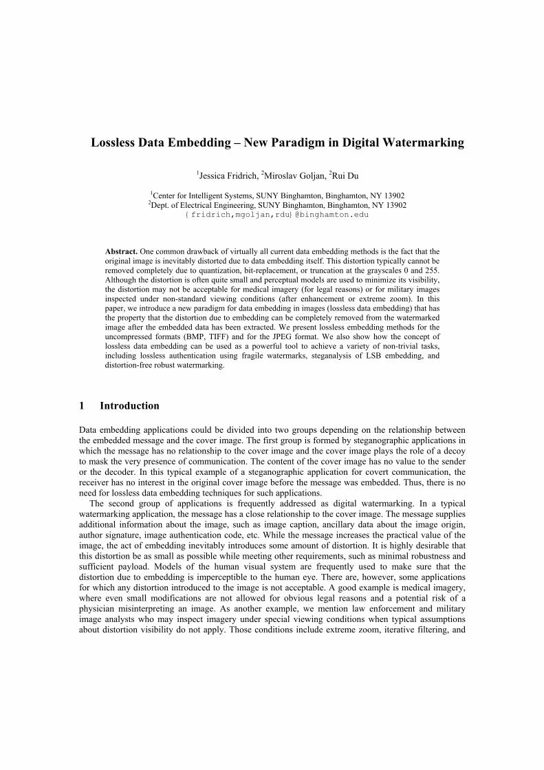
Figure 1 Diagram for lossless data embedding using lossless compression.

In an attempt to develop a general lossless data embedding technique that would be extendable to all

formats while providing large capacity and small distortion, we proposed the following paradigm [1,3]. Let us assume that there exists a subset B in the original image I, such that B can be losslessly compressed (using some lossless data compression method), and at the same time, B can be randomized without causing perceptible changes to the original image I (see Figure 1). If such a subset can be found, then we can embed data losslessly by replacing the set B with its compressed form C(B) and a message M. The capacity of this method is |B| − |C(B)|, where |x| denotes the cardinality of x. In our previous paper [1], we proposed using bit-planes as the set B. However, in this method higher payloads forced us to use higher bit-planes, thus quickly increasing the distortion in the image beyond an acceptable level. A much more elegant and effective solution is the RS data embedding [5] elaborated upon in Section 3.

The general methodology described in Figure 1 is equally applicable to lossy formats. Actually, it is easier to identify a suitable subset B for the JPEG format than for uncompressed formats, such as the BMP or TIFF formats. The lossless data embedding methods for JPEG images are detailed in Section 4.

3 The RS Lossless Data Embedding Method for Uncompressed Image Formats

Let us assume that the original image is a grayscale image with M×N pixels and with pixel values from the set P. For example, for an 8-bit grayscale image, P = {0, …, 255}. We start with dividing the image into disjoint groups of n adjacent pixels (x1, …, xn). For example, we can choose groups of n=4 consecutive pixels in a row. We also define so called discrimination function f that assigns a real number f(x1, …, xn)∈R to each pixel group G = (x1, …, xn). The purpose of the discrimination function is to capture the smoothness or "regularity" of the group of pixels G. As pointed out at the end of Section 4, image models or statistical assumptions about the original image can be used for the design of discrimination functions. For example, we can choose the 'variation' of the group of pixels (x1, …, xn) as the discrimination function f:

∑−

=+ −=

1

1121 ),...,,(

n

iiin xxxxxf . (1)

Finally, we define an invertible operation F on P called "flipping". Flipping is a permutation of gray

levels that entirely consists of two-cycles. Thus, F will have the property that F2 = Identity or F(F(x)) = x for all x∈P. For example, the permutation FLSB defined as 0 ↔ 1, 2 ↔ 3, …, 254 ↔ 255 corresponds to flipping (negating) the LSB of each gray level. The permutation 0 ↔ 2, 1 ↔ 3, 4 ↔ 6, 5 ↔ 7, … corresponds to an invertible noise with a larger “amplitude”. One can easily visualize that many possible flipping permutations are possible, including those in which the flipping is irregular with several different changes in gray scales rather than just one. A useful numerical characteristic for the permutation F is its "amplitude". The amplitude A of the flipping permutation F is defined as the average change of x under the application of F:

∑∈

−=Px

xFxP

A )(1 . (2)

For FLSB the amplitude is 1. The other permutation from the previous paragraph has A = 2. Larger values of the amplitude A correspond to adding more noise after applying F.

We use the discrimination function f and the flipping operation F to define three types of pixel groups: R, S, and U

Regular groups: G ∈ R ⇔ f(F(G)) > f(G) Singular groups: G ∈ S ⇔ f(F(G)) < f(G) Unusable groups: G ∈ U ⇔ f(F(G)) = f(G).

In the expression F(G), the flipping function F is applied to all (or selected) components of the vector G=(x1, …, xn). The noisier the group of pixels G=(x1, …, xn) is, the larger the value of the discrimination function becomes. The purpose of the flipping F is perturbing the pixel values in an invertible way by some small amount thus simulating the act of "invertible noise adding". In typical pictures, adding small amount of noise (i.e., flipping by a small amount) will lead to an increase in the discrimination function rather than decrease. Although this bias may be quite small, it will enable us to embed a large amount of information in an invertible manner.

Having explained the logic behind the definitions, we now outline the principle of the new lossless high-capacity data embedding method. Let us denote the number of regular, singular, and unusable groups in the image as NR, NS, and NU, respectively. We have NR+NS+NU = MN/n. Because real images have spatial structures, we expect a bias between the number of regular groups and singular groups: NR > NS. As will be seen below, this bias will enable us to losslessly embed data. We further note that

if G is regular, F(G) is singular, if G is singular, F(G) is regular, and if G is unusable, F(G) is unusable.

Thus, the R and S groups are flipped into each other under the flipping operation F, while the unusable groups U do not change their status. In a symbolic form, F(R)=S, F(S)=R, and F(U)=U.

We can now formulate the data embedding method. By assigning a 1 to R and a 0 to S we embed one message bit in each R or S group. If the message bit and the group type do not match, we apply the flipping operation F to the group to obtain a match. We cannot use all R and S groups for the payload because we need to be able to revert to the exact original image after we extract the data at the receiving end. To solve this problem, we use an idea similar to the one proposed in our previous paper [1]. Before

the embedding starts, we scan the image by groups and losslessly compress the status of the image − the bit-stream of R and S groups (the RS-vector) with the U groups simply skipped. We do not need to include the U groups, because they do not change in the process of message embedding and can be all unambiguously identified and skipped during embedding and extraction. We take the compressed RS-vector C, append the message bits to it, and embed the resulting bit-stream in the image using the process described above.

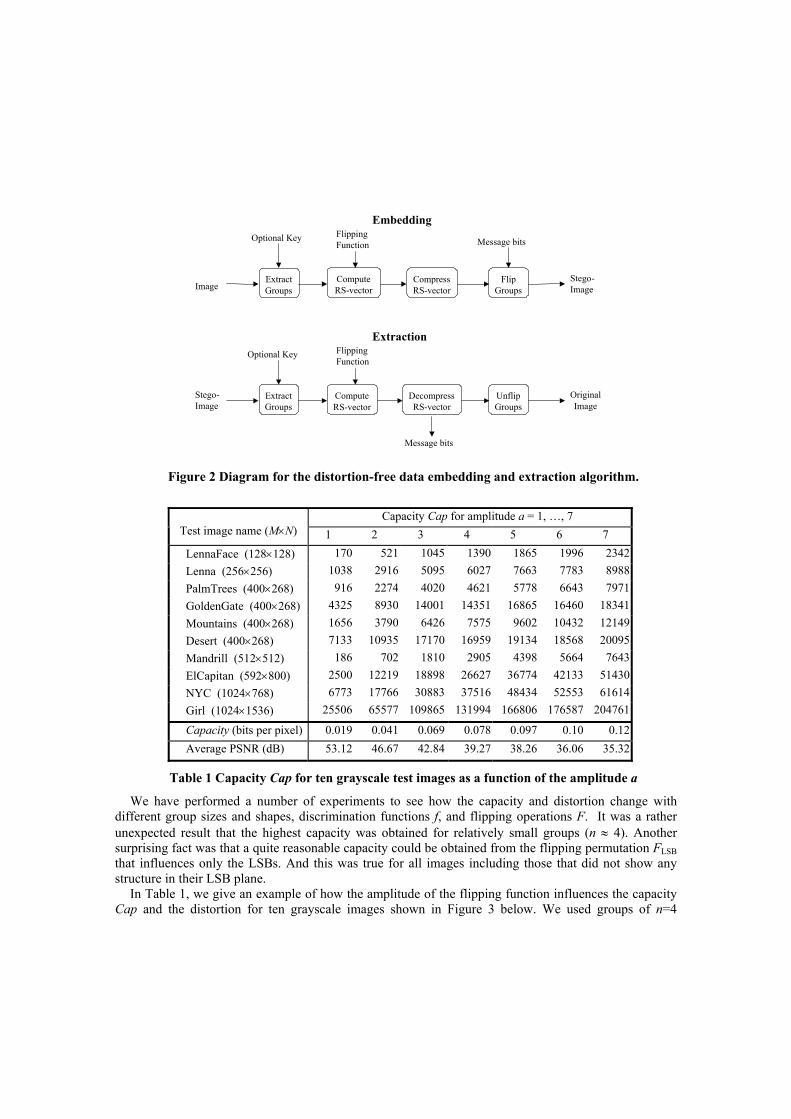
At the receiving end, the user simply extracts the bit-stream from all R and S groups (R=1, S=0) by scanning the image in the same order as during the embedding. The extracted bit-stream is separated into the message and the compressed RS-vector C. The bit-stream C is decompressed to reveal the original status of all R and S groups. The image is then processed and the status of all groups is adjusted as necessary by flipping the groups back to their original state. Thus, the exact copy of the original image is obtained. The block diagram of the embedding and extracting procedure is given in Figure 2 below.

The raw information capacity for this data embedding method is NR+NS = MN/n − NU bits. However, because we need to store the message and the compressed bit-stream C, the real capacity Cap that can be used for the message is

|| CNNCap SR −+= ,

where |C| is the length of the bit-stream C. As the bias between R and S groups increases, the compressed bit-stream C becomes shorter and the capacity higher. An ideal lossless context-free compression scheme (the entropy coder [9]) would compress the RS-vector consisting of NR+NS bits using

+

−

+

−SR

SS

SR

RR NN

NN

NNN

N loglog bits.

As a result, we obtain

.loglog

+

+

+

++=SR

SS

SR

RRSR NN

NNNN

NNNNCap

This estimate will be positive whenever there is a bias between the number of R and S groups, or when

NR ≠ NS. This bias is influenced by the size and shape of the group G, the discrimination function f, the amplitude of the flipping F, and the content of the original image. The bias increases with the group size n and the amplitude of the permutation F. Smoother and less noisy images lead to a larger bias than images that are highly textured or noisy.

The bias is not, however the parameter that should be optimized for this scheme. The capacity Cap is the characteristic that should be maximized to obtain the best performance. Our goal is to choose such a combination of the group size n and its shape, the permutation F, and the discrimination function f, in order to maximize the capacity while keeping the distortion to the image as small as possible. The expression for the capacity Cap was experimentally verified on test images using the adaptive arithmetic coder [9] as the lossless compression. It was found that Cap matched the achieved bit-rate within 15−30 bits depending on the image size.

Message bits

Image

Optional Key

Stego-Image

ExtractGroups

ComputeRS-vector

CompressRS-vector

FlipGroups

FlippingFunction

Message bits

Stego-Image

OriginalImage

ExtractGroups

ComputeRS-vector

DecompressRS-vector

UnflipGroups

FlippingFunction

Embedding

ExtractionOptional Key

Figure 2 Diagram for the distortion-free data embedding and extraction algorithm.

Capacity Cap for amplitude a = 1, …, 7

Test image name (M×N) 1 2 3 4 5 6 7 LennaFace (128×128) 170 521 1045 1390 1865 1996 2342 Lenna (256×256) 1038 2916 5095 6027 7663 7783 8988 PalmTrees (400×268) 916 2274 4020 4621 5778 6643 7971 GoldenGate (400×268) 4325 8930 14001 14351 16865 16460 18341 Mountains (400×268) 1656 3790 6426 7575 9602 10432 12149 Desert (400×268) 7133 10935 17170 16959 19134 18568 20095 Mandrill (512×512) 186 702 1810 2905 4398 5664 7643 ElCapitan (592×800) 2500 12219 18898 26627 36774 42133 51430 NYC (1024×768) 6773 17766 30883 37516 48434 52553 61614 Girl (1024×1536) 25506 65577 109865 131994 166806 176587 204761

Capacity (bits per pixel) 0.019 0.041 0.069 0.078 0.097 0.10 0.12 Average PSNR (dB) 53.12 46.67 42.84 39.27 38.26 36.06 35.32

Table 1 Capacity Cap for ten grayscale test images as a function of the amplitude a

We have performed a number of experiments to see how the capacity and distortion change with different group sizes and shapes, discrimination functions f, and flipping operations F. It was a rather unexpected result that the highest capacity was obtained for relatively small groups (n ≈ 4). Another surprising fact was that a quite reasonable capacity could be obtained from the flipping permutation FLSB that influences only the LSBs. And this was true for all images including those that did not show any structure in their LSB plane.

In Table 1, we give an example of how the amplitude of the flipping function influences the capacity Cap and the distortion for ten grayscale images shown in Figure 3 below. We used groups of n=4

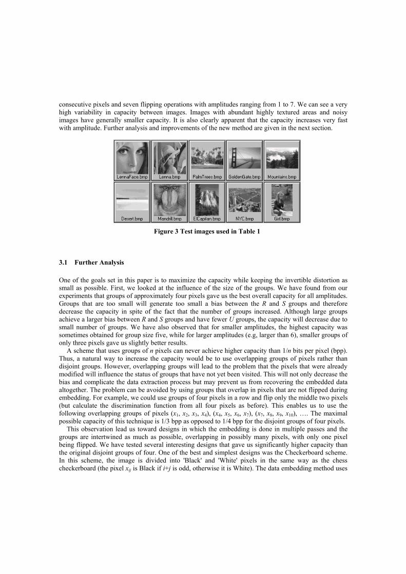
consecutive pixels and seven flipping operations with amplitudes ranging from 1 to 7. We can see a very high variability in capacity between images. Images with abundant highly textured areas and noisy images have generally smaller capacity. It is also clearly apparent that the capacity increases very fast with amplitude. Further analysis and improvements of the new method are given in the next section.

Figure 3 Test images used in Table 1

3.1 Further Analysis

One of the goals set in this paper is to maximize the capacity while keeping the invertible distortion as small as possible. First, we looked at the influence of the size of the groups. We have found from our experiments that groups of approximately four pixels gave us the best overall capacity for all amplitudes. Groups that are too small will generate too small a bias between the R and S groups and therefore decrease the capacity in spite of the fact that the number of groups increased. Although large groups achieve a larger bias between R and S groups and have fewer U groups, the capacity will decrease due to small number of groups. We have also observed that for smaller amplitudes, the highest capacity was sometimes obtained for group size five, while for larger amplitudes (e.g, larger than 6), smaller groups of only three pixels gave us slightly better results.

A scheme that uses groups of n pixels can never achieve higher capacity than 1/n bits per pixel (bpp). Thus, a natural way to increase the capacity would be to use overlapping groups of pixels rather than disjoint groups. However, overlapping groups will lead to the problem that the pixels that were already modified will influence the status of groups that have not yet been visited. This will not only decrease the bias and complicate the data extraction process but may prevent us from recovering the embedded data altogether. The problem can be avoided by using groups that overlap in pixels that are not flipped during embedding. For example, we could use groups of four pixels in a row and flip only the middle two pixels (but calculate the discrimination function from all four pixels as before). This enables us to use the following overlapping groups of pixels (x1, x2, x3, x4), (x4, x5, x6, x7), (x7, x8, x9, x10), …. The maximal possible capacity of this technique is 1/3 bpp as opposed to 1/4 bpp for the disjoint groups of four pixels.

This observation lead us toward designs in which the embedding is done in multiple passes and the groups are intertwined as much as possible, overlapping in possibly many pixels, with only one pixel being flipped. We have tested several interesting designs that gave us significantly higher capacity than the original disjoint groups of four. One of the best and simplest designs was the Checkerboard scheme. In this scheme, the image is divided into 'Black' and 'White' pixels in the same way as the chess checkerboard (the pixel xij is Black if i+j is odd, otherwise it is White). The data embedding method uses

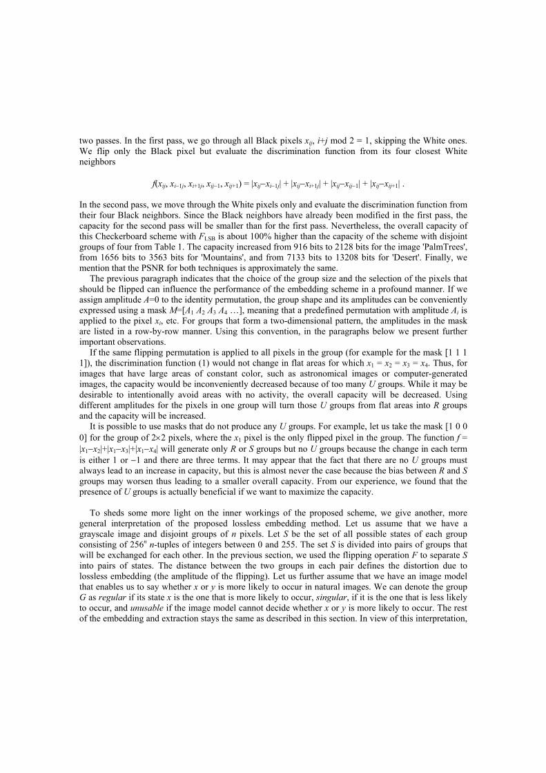
two passes. In the first pass, we go through all Black pixels xij, i+j mod 2 = 1, skipping the White ones. We flip only the Black pixel but evaluate the discrimination function from its four closest White neighbors

f(xij, xi−1j, xi+1j, xij−1, xij+1) = |xij−xi−1j| + |xij−xi+1j| + |xij−xij−1| + |xij−xij+1| .

In the second pass, we move through the White pixels only and evaluate the discrimination function from their four Black neighbors. Since the Black neighbors have already been modified in the first pass, the capacity for the second pass will be smaller than for the first pass. Nevertheless, the overall capacity of this Checkerboard scheme with FLSB is about 100% higher than the capacity of the scheme with disjoint groups of four from Table 1. The capacity increased from 916 bits to 2128 bits for the image 'PalmTrees', from 1656 bits to 3563 bits for 'Mountains', and from 7133 bits to 13208 bits for 'Desert'. Finally, we mention that the PSNR for both techniques is approximately the same.

The previous paragraph indicates that the choice of the group size and the selection of the pixels that should be flipped can influence the performance of the embedding scheme in a profound manner. If we assign amplitude A=0 to the identity permutation, the group shape and its amplitudes can be conveniently expressed using a mask M=[A1 A2 A3 A4 …], meaning that a predefined permutation with amplitude Ai is applied to the pixel xi, etc. For groups that form a two-dimensional pattern, the amplitudes in the mask are listed in a row-by-row manner. Using this convention, in the paragraphs below we present further important observations.

If the same flipping permutation is applied to all pixels in the group (for example for the mask [1 1 1 1]), the discrimination function (1) would not change in flat areas for which x1 = x2 = x3 = x4. Thus, for images that have large areas of constant color, such as astronomical images or computer-generated images, the capacity would be inconveniently decreased because of too many U groups. While it may be desirable to intentionally avoid areas with no activity, the overall capacity will be decreased. Using different amplitudes for the pixels in one group will turn those U groups from flat areas into R groups and the capacity will be increased.

It is possible to use masks that do not produce any U groups. For example, let us take the mask [1 0 0 0] for the group of 2×2 pixels, where the x1 pixel is the only flipped pixel in the group. The function f = |x1−x2|+|x1−x3|+|x1−x4| will generate only R or S groups but no U groups because the change in each term is either 1 or −1 and there are three terms. It may appear that the fact that there are no U groups must always lead to an increase in capacity, but this is almost never the case because the bias between R and S groups may worsen thus leading to a smaller overall capacity. From our experience, we found that the presence of U groups is actually beneficial if we want to maximize the capacity.

To sheds some more light on the inner workings of the proposed scheme, we give another, more

general interpretation of the proposed lossless embedding method. Let us assume that we have a grayscale image and disjoint groups of n pixels. Let S be the set of all possible states of each group consisting of 256n n-tuples of integers between 0 and 255. The set S is divided into pairs of groups that will be exchanged for each other. In the previous section, we used the flipping operation F to separate S into pairs of states. The distance between the two groups in each pair defines the distortion due to lossless embedding (the amplitude of the flipping). Let us further assume that we have an image model that enables us to say whether x or y is more likely to occur in natural images. We can denote the group G as regular if its state x is the one that is more likely to occur, singular, if it is the one that is less likely to occur, and unusable if the image model cannot decide whether x or y is more likely to occur. The rest of the embedding and extraction stays the same as described in this section. In view of this interpretation,

the discrimination function (1) is a special case of an embodiment of an image model derived from the assumption that groups with smaller variance are more likely to occur than groups with higher variance.

3.2 Experimental Results

To obtain a better understanding of how different components and parameters affect the performance of the proposed lossless data embedding method, we present some results in a graphical form. All experiments were performed with five small grayscale test images ('Lenna' with 256×256 pixels, 'PalmTrees', 'GoldenGate', 'Mountains', with 400×268 pixels, and 'NYC' at the resolution 1024×768).

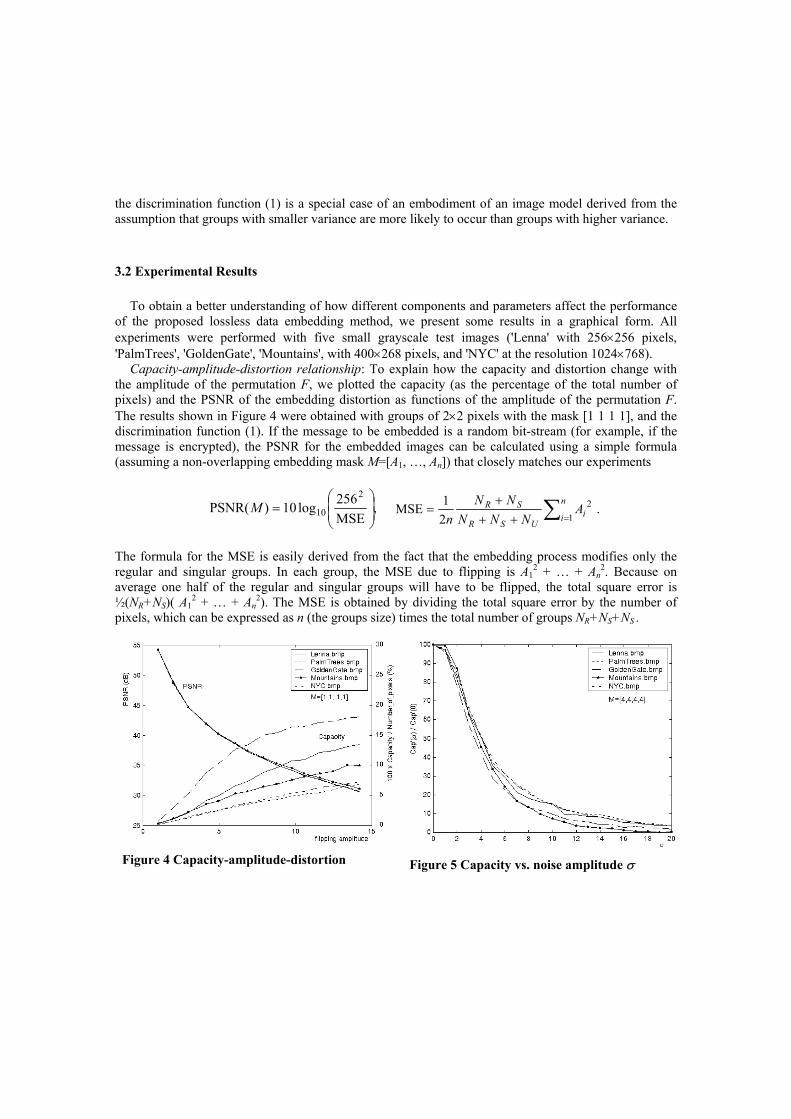
Capacity-amplitude-distortion relationship: To explain how the capacity and distortion change with the amplitude of the permutation F, we plotted the capacity (as the percentage of the total number of pixels) and the PSNR of the embedding distortion as functions of the amplitude of the permutation F. The results shown in Figure 4 were obtained with groups of 2×2 pixels with the mask [1 1 1 1], and the discrimination function (1). If the message to be embedded is a random bit-stream (for example, if the message is encrypted), the PSNR for the embedded images can be calculated using a simple formula (assuming a non-overlapping embedding mask M=[A1, …, An]) that closely matches our experiments

,MSE256log10)PSNR(

2

10

=M ∑=++

+=

n

i iUSR

SR ANNN

NNn 1

2

21MSE .

The formula for the MSE is easily derived from the fact that the embedding process modifies only the regular and singular groups. In each group, the MSE due to flipping is A1

2 + … + An2. Because on

average one half of the regular and singular groups will have to be flipped, the total square error is ½(NR+NS)( A1

2 + … + An2). The MSE is obtained by dividing the total square error by the number of

pixels, which can be expressed as n (the groups size) times the total number of groups NR+NS+NS .

Figure 4 Capacity-amplitude-distortion Figure 5 Capacity vs. noise amplitude σ

Capacity vs. noise: Figure 5 shows how the capacity depends on the amount of noise added to the original image. The x axis is the standard deviation σ of a white i.i.d. Gaussian noise added to the image and the y axis is the ratio Cap'(σ)/Cap'(0) between the capacity after adding noise with amplitude σ and the capacity for the original image without any added noise. The results correspond to the mask [4,4,4,4] with the discrimination function (1). The PSNR after message embedding was always in the range 39−40 dB. We note that the presence of noise decreases the capacity in a gradual rather than an abrupt way. Also, the capacity remains in hundreds of bits even for images that contain very visible noise.

4 Lossless Data Embedding for JPEG Images

In this section, we describe two lossless data embedding techniques for JPEG images. The data is embedded in the quantized DCT coefficients in an invertible way so that it is possible to reconstruct from the watermarked image the exact copy of the original image. In the first technique, the subset B with compressible structure is the set of all LSBs of one selected quantized DCT coefficient from all blocks. This set is obviously easily compressible (biased towards zero) but can be randomized without introducing disturbing distortion. The second method, that we present, is based on a simple trick used to preprocess the original image to enable trivial lossless data embedding.

4.1 Method 1

Although in this paper, we explain the techniques on grayscale images, the technology can be extended to color images in a straightforward manner. The JPEG compression starts with dividing the image into disjoint blocks of 8×8 pixels. For each block, the discrete cosine transform (DCT) is calculated, producing 64 DCT coefficients. Let us denote the (i,j)-th DCT coefficient of the k-th block as dk(i,j), 0 ≤ i, j ≤ 64, k = 1, …, b, where b is the total number of blocks in the image. In each block, all 64 coefficients are further quantized to integers Dk(i,j) with a JPEG quantization matrix Q

=

),(),(

_),(jiQjid

roundintegerjiD kk .

The quantized coefficients are arranged in a zig-zag manner and compressed using the Huffman coder. The resulting compressed stream together with a header forms the final JPEG file.

The largest DCT coefficients occur for the lowest frequencies (small i and j). Due to properties of

typical images and due to quantization, the quantized DCT coefficients corresponding to higher frequencies have a large number of zeros or small integers, such as 1's or −1's. For example, for the classical grayscale test image 'Lenna' with 256×256 pixels, the DCT coefficient (5,5) is zero in 94.14% of all blocks. In 2.66% cases it is a 1, and in 2.81% cases it is equal to −1, with less than 1% of 2's and −2's. Thus, the sequence Dk(5,5) forms a subset B that is easily compressible with the Huffman or arithmetic coder. Furthermore, if we embed message bits into the LSBs of the coefficients Dk(5,5), we only need to compress the original LSBs of the sequence Dk(5,5) instead of the coefficient values. We can further improve the efficiency of the algorithm if we define the LSB of negative integers Dk < 0 as

LSB(Dk) = 1 − (|Dk| mod 2). Thus, LSB(−1)=LSB(−3)=0, and LSB(−2)=LSB(−4)=1, etc. Because DCT coefficients Dk have a symmetrical distribution with zero mean, this simple measure will increase the bias between zeros and ones in the LSB bit-stream of original DCT coefficients. With an increased bias, the lossless capacity will also be higher.

DCT coefficients Dk(i,j) corresponding to higher-frequencies will produce a set B with a larger bias

between zeros and ones, but because the quantization factor Q(i,j) is higher for such coefficients, the distortion in each modified block will also be higher. To obtain the best results, one should use different DCT coefficients for different JPEG quality factors to minimize the overall distortion and avoid introducing visible artifacts. As a good overall choice, we recommend the coefficients corresponding to the middle frequencies. For color images, embedding into the chrominance channels introduces much less visible distortion than embedding into the luminance component.

Below, we give a pseudo-code for lossless data embedding of grayscale JPEG images. Lossless data embedding in JPEG images (Method 1)

1. Based on the JPEG quality factor, determine the set of L pairs of indices (i1,j1), (i2,j2), …, (iL,jL), 0 ≤ il, jl ≤ 64, corresponding to middle frequencies.

2. Read the JPEG file and use the Huffman decompressor to obtain the values of quantized DCT coefficients, Dk(i,j), 0 ≤ i, j ≤ 64, k = 1, …, b, where b is the total number of blocks in the image.

3. Seed a PRNG with a secret key and follow a random non-intersecting walk through the set S={D1(i1,j1), …, Db(i1,j1), D1(i2,j2), …, Db(i2,j2), …, D1(iL,jL), …, Db(iL,jL)}. There are L×b elements in the set S.

4. While following the random walk, run the adaptive context-free lossless arithmetic compression algorithm for the LSBs of the coefficients from S (e.g., compress the set B of LSBs). While compressing, check for the difference between the length of the compressed bit-stream C and the number of processed coefficients. Once there is enough space to insert the message, stop running the compression algorithm. Denote the set of visited coefficients as S1, S1 ⊆ S.

5. Concatenate the compressed bit-stream C and the message and insert the resulting bit-stream into the LSBs of the coefficients from S1. Huffman compress all DCT coefficients Dk(i,j) including the modified ones and store the watermarked image as a JPEG file on a disk.

Message extraction and recovery of the original image (Method 1)

1. Based on the JPEG quality factor, determine the set of L of pairs of indices (i1,j1), (i2,j2), …, (iL,jL), 0 ≤ il, jl ≤ 64.

2. Read the JPEG file and use Huffman decompressor to obtain the values of quantized DCT coefficients, Dk(i,j), 0 ≤ i, j ≤ 64, k = 1, …, b.

3. Seed a PRNG with a secret key and follow a random non-intersecting walk through the set S={D1(i1,j1), …, Db(i1,j1), D1(i2,j2), …, Db(i2,j2), …, D1(iL,jL), …, Db(iL,jL)}.

4. While following the random walk, run the context-free lossless arithmetic decompression algorithm for the LSBs of the coefficients visited during the random walk. Once the length of the decompressed bit-stream reaches b + message_length (the message length should be embedded in the header of the message), stop Step 4.

5. Separate the decompressed bit-stream into the LSBs of visited DCT coefficients and the message. Replace the LSBs of all visited coefficients with the decompressed bit-stream to obtain the original image.

The selection of the L DCT coefficients can be adjusted according to the quality factor to minimize the

distortion and other artifacts. For example, using L=3 coefficients (5,5), (4,6), and (6,3) in a random fashion will contribute to the overall security of the scheme because the statistical artifacts due to lossless authentication will be more difficult to detect.

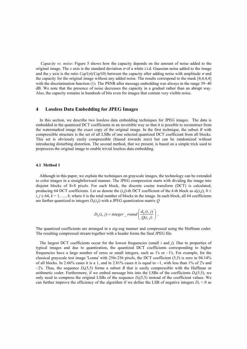
Table 2 below shows the distortion measured using the PSNR. For simplicity, in our experiments we used one fixed DCT coefficient (6,6) and three color test images. The JPEG images were obtained by saving raw bitmaps as JPEGs with four different quality factors in PaintShop Pro 4.12.

Distortion (dB) Test image

JPEG 90% JPEG 85% JPEG 75% JPEG 50% P1 (512×330) 55.0 (42.0) 52.0 (38.8) 48.0 (34.6) 43.0 (28.8) P2 (256×256) 50.5 (38.6) 47.8 (35.3) 44.0 (30.0) 37.6 (25.2) P3 (878×586) 59.7 (46.4) 56.6 (43.3) 53.6 (39.2) 47.2 (33.4)

Table 2 Distortion for lossless embedding of 128 (4000) bits for three test images P1, P2, P3, and different JPEG quality factors

4.2 Method 2

The idea for the second method is quite simple. If, for a given DCT coefficient (i,j), the quantization factor Q(i,j) is even, we could divide it by two and multiply all coefficients Dk(i,j) by two without changing the visual appearance of the image at all. Because now all Dk(i,j) are even, we can embed any binary message into the LSBs of Dk(i,j) and this LSB embedding will be trivially invertible (the bias between zeros and ones is infinite).

If Q(i,j) is odd, we replace it with floor(Q(i,j)/2) and multiply all Dk(i,j) by two. In this case, we need to include a flag to the message telling us that Q(i,j) was originally odd in order to be able to reconstruct the original JPEG stream during message extraction. Because this method uses a non-standard quantization table, the table must be included in the header of the authenticated image. Because the table entry Q(i,j) will not be compatible with the rest of the table, it will be easy to tell whether or not a given JPEG image has been authenticated by this method, i.e., the method is steganographically obvious.

Figure 6 Three color test images P1, P2, and P3

Method 2a Dk(i,j)→ Dk(i,j)/2 Method 2b Dk(i,j)→ 1

Image QF (6,6) (5,4) (4,2) (6,6) (5,4) (4,2) 50 49.3 (34.7) 46.5 (32.3) 49.2 (33.2) 66.6 (54.4) 66.2 (54.6) 66.6 (54.2) 75 54.6 (40.4) 52.0 (38.0) 52.9 (39.1) 66.9 (55.0) 66.5 (55.2) 67.0 (54.8) 85 58.0 (44.4) 55.6 (42.1) 57.0 (43.1) 66.5 (55.0) 66.0 (55.0) 66.6 (54.8)

P1

512×330 90 60.4 (47.1) 58.6 (45.1) 58.7 (46.3) 66.9 (55.1) 66.7 (55.1) 67.0 (54.7) 50 43.7 (31.1) 40.8 (28.2) 43.2 (27.1) 62.0 (53.5) 61.8 (53.1) 62.0 (52.7) 75 50.8 (37.1) 48.1 (34.3) 49.0 (32.9) 62.7 (53.5) 62.2 (53.0) 62.5 (52.5) 85 54.1 (41.2) 51.5 (38.5) 53.1 (37.2) 62.3 (53.5) 61.8 (53.0) 62.5 (52.6)

P2

256×256 90 56.0 (44.3) 54.0 (41.8) 54.7 (40.7) 62.5 (53.5) 62.3 (53.1) 62.2 (52.5) 50 53.6 (39.4) 50.7 (36.4) 53.3 (38.4) 70.8 (56.8) 70.3 (56.4) 70.6 (56.7) 75 59.2 (44.8) 56.6 (42.0) 57.6 (44.2) 71.4 (57.8) 71.4 (57.4) 71.8 (57.7) 85 62.7 (48.4) 60.3 (45.8) 61.7 (47.5) 71.4 (58.0) 70.6 (57.6) 71.2 (57.9)

P3

878×586 90 64.9 (50.5) 63.0 (48.5) 61.7 (50.4) 71.7 (58.1) 71.5 (57.7) 71.6 (57.9)

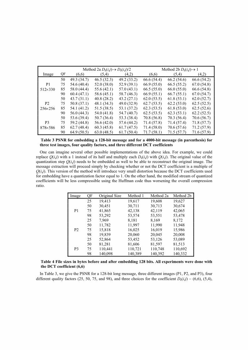
Table 3 PSNR for embedding a 128-bit message and for a 4000-bit message (in parenthesis) for three test images, four quality factors, and three different DCT coefficients

One can imagine several other possible implementations of the above idea. For example, we could replace Q(i,j) with a 1 instead of its half and multiply each Dk(i,j) with Q(i,j). The original value of the quantization step Q(i,j) needs to be embedded as well to be able to reconstruct the original image. The message extraction will proceed simply by checking whether or not the DCT coefficient is a multiple of Q(i,j). This version of the method will introduce very small distortion because the DCT coefficients used for embedding have a quantization factor equal to 1. On the other hand, the modified stream of quantized coefficients will be less compressible using the Huffman code thus worsening the overall compression ratio.

Image QF Original Size Method 1 Method 2a Method 2b 25 19,413 19,617 19,608 19,627 50 30,451 30,711 30,713 30,674 75 41,865 42,138 42,119 42,065

P1 98 53,292 53,574 53,551 53,478 25 7,969 8,181 8,169 8,172 50 11,782 11,997 11,990 11,948 75 15,818 16,025 16,019 15,986

P2 98 19,839 20,060 20,045 20,008 25 52,864 53,452 53,126 53,089 50 81,281 81,606 81,597 81,513 75 110,441 110,721 110,748 110,692

P3 98 140,098 140,389 140,392 140,332

Table 4 File sizes in bytes before and after embedding 128 bits. All experiments were done with the DCT coefficient (6,6)

In Table 3, we give the PSNR for a 128-bit long message, three different images (P1, P2, and P3), four different quality factors (25, 50, 75, and 98), and three choices for the coefficient Dk(i,j) − (6,6), (5,4),

and (4,2), and three color images. The numbers in parenthesis correspond to a 4000 bit message. Table 4 shows the file sizes before and after embedding for the coefficient (6,6).

5 Applications

5.1 Lossless authentication

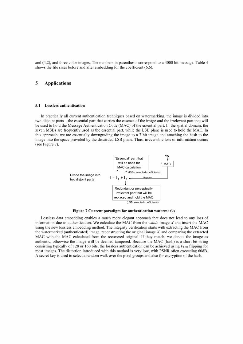
In practically all current authentication techniques based on watermarking, the image is divided into two disjoint parts – the essential part that carries the essence of the image and the irrelevant part that will be used to hold the Message Authentication Code (MAC) of the essential part. In the spatial domain, the seven MSBs are frequently used as the essential part, while the LSB plane is used to hold the MAC. In this approach, we are essentially downgrading the image to a 7 bit image and attaching the hash to the image into the space provided by the discarded LSB plane. Thus, irreversible loss of information occurs (see Figure 7).

I = I 1 + I 2

“Essential” part thatwill be used for

MAC calculation

Redundant or perceptuallyirrelevant part that will be

replaced and hold the MAC

(7 MSBs, selected coefficients)

(LSB, selected coefficients)

Key

MAC

ReplaceDivide the image into two disjoint parts

Figure 7 Current paradigm for authentication watermarks

Lossless data embedding enables a much more elegant approach that does not lead to any loss of information due to authentication. We calculate the MAC from the whole image X and insert the MAC using the new lossless embedding method. The integrity verification starts with extracting the MAC from the watermarked (authenticated) image, reconstructing the original image X, and comparing the extracted MAC with the MAC calculated from the recovered original. If they match, we denote the image as authentic, otherwise the image will be deemed tampered. Because the MAC (hash) is a short bit-string consisting typically of 128 or 160 bits, the lossless authentication can be achieved using FLSB flipping for most images. The distortion introduced with this method is very low, with PSNR often exceeding 60dB. A secret key is used to select a random walk over the pixel groups and also for encryption of the hash.

5.2 Steganalysis of LSB embedding

Capacity Cap can be used as a sensitive measure for detecting image modifications, such as those due to data hiding or steganography. In this paragraph, we outline an idea how to detect LSB embedding for grayscale images. LSB embedding in grayscale images is relatively hard to detect for a number of reasons. The method based on Pairs of Values and χ2-statistics as introduced by Westfeld [10] becomes only reliable when either the data is embedded in consecutive pixels, or when the message length is comparable to the image size (in the case of embedding along a random walk). Their method will not give reliable results even for secret messages of size 50% of the pixel number. The method [2] was designed for color images and relies on pairs of close colors. It becomes completely ineffective for grayscale images.

We note that even very noisy images with LSB planes that do not show any structure or regularity have a non-zero capacity Cap in the LSB plane. The most important observation that enables reliable and very accurate detection of LSB embedding is the fact that the capacity for the LSB flipping decreases with increased message size embedded in the LSB plane, while the capacity for the shifted LSB flipping (0, 1 ↔ 2, 3 ↔ 4, …, 253 ↔ 254, 255) increases. By embedding messages in the LSB plane into the image under inspection and observing the decrease in lossless capacity in the LSB plane and increase in the shifted LSB plane, we can accurately estimate the degree of randomization of the LSB plane – the secret message length. Detailed exposition of this idea can be found in our paper solely devoted to steganalysis [4].

5.3 Distortion-free robust watermarking

A distortion-free robust watermark is a robust watermark that can be completely removed from the watermarked image if no distortion occurred to it. For such a watermark, there is no need to store both the original image and its watermarked version because the original can be obtained from the watermarked image. Storing only the watermarked version will also give an attacker less space to mount an attack in case she gets access to the computer system.

Spatial additive non-adaptive watermarking schemes in which the watermarked image Xw is obtained by adding the watermark pattern W(Key,Payload) to the original image X are almost invertible except for the loss of information due to truncation at the boundary of the dynamic range (i.e., at 0 and 255 for grayscale images). We propose to not modify those pixels that would over/underflow after watermark adding. Assuming we have Y(i,j) = X(i,j) + W(i,j) for every pixel (i,j):

X'w(i,j) = Y(i,j) if Y(i,j) ∈ [0,255], X'w(i,j) = X(i,j) if Y(i,j) < 0, X'w(i,j) = X(i,j) if Y(i,j) > 255.

In typical images, the set of such pixels will be relatively small and could be compressed efficiently in a lossless manner. This information along with watermark strength and other parameters used for watermark construction is then embedded in the watermarked image X'w using our lossless data embedding method.

If the resulting image is not modified, one can revert to the exact original image because after reading the watermark payload, we can generate the watermark pattern W and subtract it from all pixels except for those whose indices were recovered from the losslessly embedded data. Preliminary experiments are

encouraging and indicate that this approach is, indeed, plausible. Further analysis of this idea will be the subject of our future research.

Applications that would benefit from the newly coined lossless data embedding in general include the whole spectrum of fragile watermarking, such as authentication watermarks or watermarks protecting the image integrity. A classical authentication watermarking scheme starts with dividing the image or its blocks into two parts – the part that carries the majority of the perceptual information and an “unimportant” part that can be randomized without causing perceptible artifacts. The perceptually important part is then hashed and the hash is inserted into the “unimportant” part. The Wong’s scheme [11] is an example of such as scheme. In this scheme, the perceptually important part consists of the 7 most significant bits, while the unimportant part is formed by the least significant bit-plane. However, this and similar approaches can be reformulated as simply decreasing the information content of the image and inserting or attaching the hash to the modified image as is done in pure cryptographic authentication methods. Thus, the advantage of embedding the hash rather than appending becomes dubious at best. The lossless data embedding enables hash insertion while retaining the information content of the image in its entirety. This is important for customers who are overly concerned with the quality of their images after information has been embedded. Some customers are simply so emotionally attached to their images that no argument about invisibility of the embedding artifacts is convincing enough. Lossless embedding techniques simply close this issue because the original data can be restored without any loss of information. This is especially true for military images, such as satellite and reconnaissance images. Actually, the lossless authentication watermarks are currently being incorporated as an integrity protection mechanism into the ISSE guard. Another application that would clearly benefit from the proposed lossless techniques is integrity protection watermark embedded inside the digital camera for imaging hardware used by forensic personnel. Establishing the integrity of evidence throughout the investigation is of paramount importance. Authentication watermarks embedded by a watermarking chip inside the digital camera have been proposed in the past. However, because the authentication process invariably modifies the image, today, the legal problems associated with watermarking prevent the spread of watermarking technology. The removable lossless authentication watermark provides an elegant solution to this sensitive issue.

6 Conclusions and Future Directions

One common drawback of virtually all image data embedding methods is the fact that the original image is inevitably distorted by some small amount of noise due to data embedding itself. This distortion typically cannot be removed completely due to quantization, bit-replacement, or truncation at the grayscales 0 and 255. Although the distortion is often quite small, it may not be acceptable for medical imagery (for legal reasons) or for military images inspected under unusual viewing conditions (after filtering or extreme zoom). In this paper, we introduced a general approach for high-capacity data embedding that we call lossless in the sense that after the embedded information is extracted from the watermarked image, we can revert to the exact copy of the original image.

For uncompressed image formats, such as the BMP or the TIFF format, we proposed so called RS method that is a fragile high-capacity data embedding technique based on embedding message bits in the status of groups of pixels. The status can be obtained using a flipping operation (a permutation of grayscales) and a discrimination (prediction) function. The flipping simulates an "invertible noise adding", while the discrimination function measures how the flipping influences the local smoothness of

the flipped group. The original status of image groups is losslessly compressed and embedded together with the message in the image. At the receiving end, the message is read as well as the original compressed status of the image. The knowledge of the original status is then used to completely remove the distortion due to data embedding. The method provides a high embedding capacity while introducing a very small and invertible distortion.

We further describe two different methods for lossless data embedding for JPEG images. The first method is based on compression of LSBs of a selected quantized DCT coefficient from all blocks. The second method uses a special trick to preprocess the image to allow trivially lossless data embedding. It is based on manipulation of the quantization table.

Finally, we describe three important applications of the lossless data embedding − lossless authentication of images, detection of LSB steganography in images, and lossless robust watermarking.

Acknowledgements

The work on this paper was partially supported by Air Force Research Laboratory, Air Force Material Command, USAF, under a research grant number F30602-00-1-0521 and partially by the AFOSR grant No. F49620-01-1-0123. The U.S. Government is authorized to reproduce and distribute reprints for Governmental purposes notwithstanding any copyright notation there on. The views and conclusions contained herein are those of the authors and should not be interpreted as necessarily representing the official policies, either expressed or implied, of Air Force Research Laboratory, the Air Force Office of Scientific Research, or the U. S. Government.

References

1. Fridrich, J., Goljan, M., Du, R.: Invertible Authentication. In: Proc. SPIE, Security and Watermarking of Multimedia Contents, San Jose, California January (2001)

2. Fridrich, J., Du, R., Long, M.: Steganalysis of LSB Encoding in Color Images. In: Proc. ICME 2000, New York City, New York, July (2000)

3. Fridrich, J., Goljan, M., Du, R.: Invertible Authentication Watermark for JPEG Files. In: Proc. ITCC, Las Vegas, Nevada, April (2001)

4. Fridrich, J., Goljan, M., Du, R.: Reliable Detection of LSB Steganography in Grayscale and Color Images, in preparation for the ACM Special Session on Multimedia Security and Watermarking, Ottawa, Canada, October 5, 2001.

5. Fridrich, J., Goljan M., and Rui Du, “Distortion-Free Data Embedding for Images”, Proc. 4th Information Hiding Workshop, Pittsburgh, PA, April (2001).

6. Honsinger, C. W., Jones, P., Rabbani, M., Stoffel, J. C.: Lossless Recovery of an Original Image Containing Embedded Data. US Patent application, Docket No: 77102/E−D (1999)

7. Honsinger, C. W.: A Robust Data Hiding Technique Based on Convolution with a Randomized Phase Carrier. In: Proc. of PICS'00, Portland, Oregon, March (2000)

8. Macq, B.: Lossless Multiresolution Transform for Image Authenticating Watermarking. In: Proc. of EUSIPCO, Tampere, Finland, September (2000)

9. Sayood, K.: Introduction to Data Compression. Morgan Kaufmann Publishers, San Francisco, California (1996) 87−94

10. Westfield, A. and Pfitzmann, A.: Attacks on Steganographic Systems. In: Proc. 3rd Information Hiding Workshop, Dresden, Germany, September (1999) 61−75

11. Wong, P. W., "A watermark for image integrity and ownership verification", Proc. IS&T PIC, Portland, Oregon, 1998.