Loss reserving techniques: past, present and future Greg Taylor Taylor Fry Consulting Actuaries & University of Melbourne Grainne McGuire Taylor Fry Consulting Actuaries Alan Greenfield Taylor Fry Consulting Actuaries

Welcome message from author
This document is posted to help you gain knowledge. Please leave a comment to let me know what you think about it! Share it to your friends and learn new things together.
Transcript

Loss reserving techniques:past, present and future
Greg TaylorTaylor Fry Consulting Actuaries &
University of Melbourne
Grainne McGuireTaylor Fry Consulting Actuaries
Alan GreenfieldTaylor Fry Consulting Actuaries

Evolution of loss reserving models

3
Overview
• Taxonomy of loss reserving models– Evolution of such
models through past to present
• Examination of one of the higher species of model in more detail
• Some predictions of future evolution

4
Classification of loss reserving models
• Taxonomy of models• Considered in Taylor (1986)
– Stochasticity– Model structure
• Macro or Micro
– Dependent variables• Paid losses or incurred losses• Claim counts modelled or not
– Explanatory variables

5
Classification of loss reserving models
• Research for subsequent book (Taylor, 2000)
• About half loss reserving literature later than 1986
• New techniques introduced• Revise classification?
6
Classification of loss reserving models
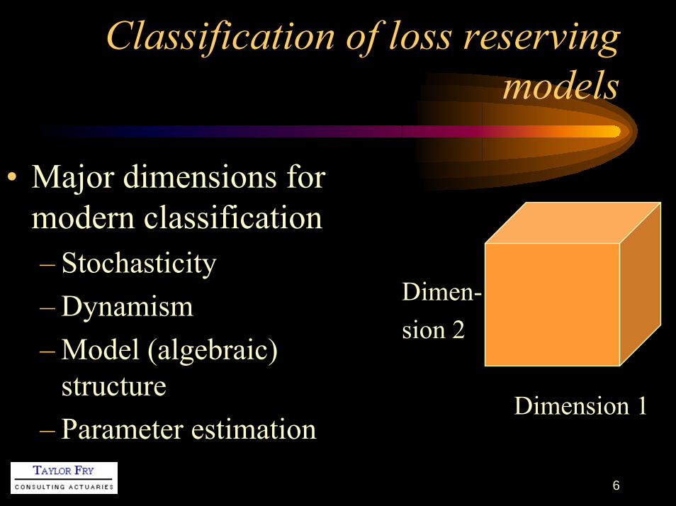
• Major dimensions for modern classification– Stochasticity– Dynamism– Model (algebraic)
structure– Parameter estimation
Dimen-sion 2
Dimension 1
7
Classification of loss reserving models
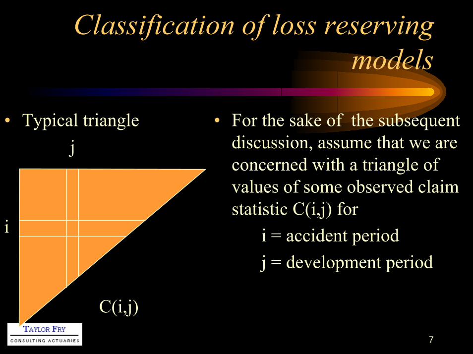
• Typical trianglej
i
C(i,j)
• For the sake of the subsequent discussion, assume that we are concerned with a triangle of values of some observed claim statistic C(i,j) for
i = accident periodj = development period

8
Classification of loss reserving models -Stochasticity
• Stochastic model– Observations C(i,j) assumed
to have formal error structure:
C(i,j) = µ(i,j) + e(i,j)
parameterstochastic error

9
Classification of loss reserving models -Dynamism
• Dynamic model– Model parameters assumed to
evolve over time
E[C(i,j)] = µ(i,j) = f (β(i),j)
parametervector
β(i) = β(i-1) + w(i)
stochasticperturbation

10
Classification of loss reserving models –Model (algebraic) structure
• Spectrum of possibilities
Phenomenological Micro-structural
Model fine structure of claims process
e.g. individual claims according to their own characteristics
Model descriptive statistics of the claims experience that have no direct physical meaning
e.g. chain ladder ratios

11
Classification of loss reserving models –Parameter estimation
• Two main possibilities– Heuristic
• e.g. chain ladder• Typical of non-stochastic models
– Optimal• i.e. according to some statistical optimality criterion• e.g. maximum likelihood

12
Evolution of loss reserving models –Phylogenetic tree
Phenomen-ological
Heuristic
Determin-istic
Phenomen-ological
Heuristic
Phenomen-ological
Micro-structural
Optimal
Stochastic
Static
Phenomen-ological
Micro-structural
Optimal
Stochastic
Dynamic
Loss reservingmodels

13
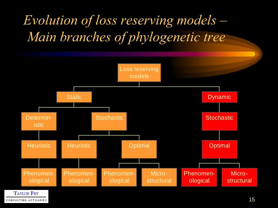
Evolution of loss reserving models –Main branches of phylogenetic tree
Phenomen-ological
Heuristic
Determin-istic
Phenomen-ological
Heuristic
Phenomen-ological
Micro-structural
Optimal
Stochastic
Static
Phenomen-ological
Micro-structural
Optimal
Stochastic
Dynamic
Loss reservingmodels

14
Evolution of loss reserving models –Main branches of phylogenetic tree
Phenomen-ological
Heuristic
Determin-istic
Phenomen-ological
Heuristic
Phenomen-ological
Micro-structural
Optimal
Stochastic
Static
Phenomen-ological
Micro-structural
Optimal
Stochastic
Dynamic
Loss reservingmodels
15
Evolution of loss reserving models –Main branches of phylogenetic tree
Phenomen-ological
Heuristic
Determin-istic
Phenomen-ological
Heuristic
Phenomen-ological
Micro-structural
Optimal
Stochastic
Static
Phenomen-ological
Micro-structural
Optimal
Stochastic
Dynamic
Loss reservingmodels

16
Darwinian view –Ascent of loss reserving models
• Earliest models (up to late 1970s)– Chain ladder (as then
viewed)– Separation method
(Taylor, 1977)– Payments per claim
finalised (Fisher & Lange, 1973; Sawkins, 1979)
– etcStatic
DeterministicPhenomenological
Heuristic

17
Darwinian view –Ascent of loss reserving models
• Any deterministic model may be stochasticised by the addition of an error term
• If error term left distribution-free, parameter estimation may still be heuristic– Stochastic chain ladder
(Mack, 1993)StaticDeterministic
PhenomenologicalHeuristic
StaticStochastic
PhenomenologicalHeuristic

18
Darwinian view –Ascent of loss reserving models
• Alternatively, optimal parameter estimation may be applied to the case of distribution-free error terms– Least squares chain ladder estimation
(De Vylder, 1978)• Optimal parameter estimation may
also be employed if error structure added– Chain ladder for triangle of Poisson
counts (Hachemeister & Stanard, 1975)
– Chain ladder with log normal age-to-age factors (Hertig, 1985)
– Chain ladder with triangle of over-dispersed Poisson cells (England & Verrall, 2002)
StaticDeterministic
PhenomenologicalHeuristic
StaticStochastic
PhenomenologicalHeuristic
StaticStochastic
PhenomenologicalOptimal

19
Darwinian view –Ascent of loss reserving models
• Insert finer structure into model– Payments per claim
finalised (Taylor & Ashe, 1983)
– Distribution of individual claim sizes at each operational time (Reid, 1978)
StaticDeterministic
PhenomenologicalHeuristic
StaticStochastic
PhenomenologicalHeuristic
StaticStochastic
Micro-structuralOptimal
StaticStochastic
PhenomenologicalOptimal
20
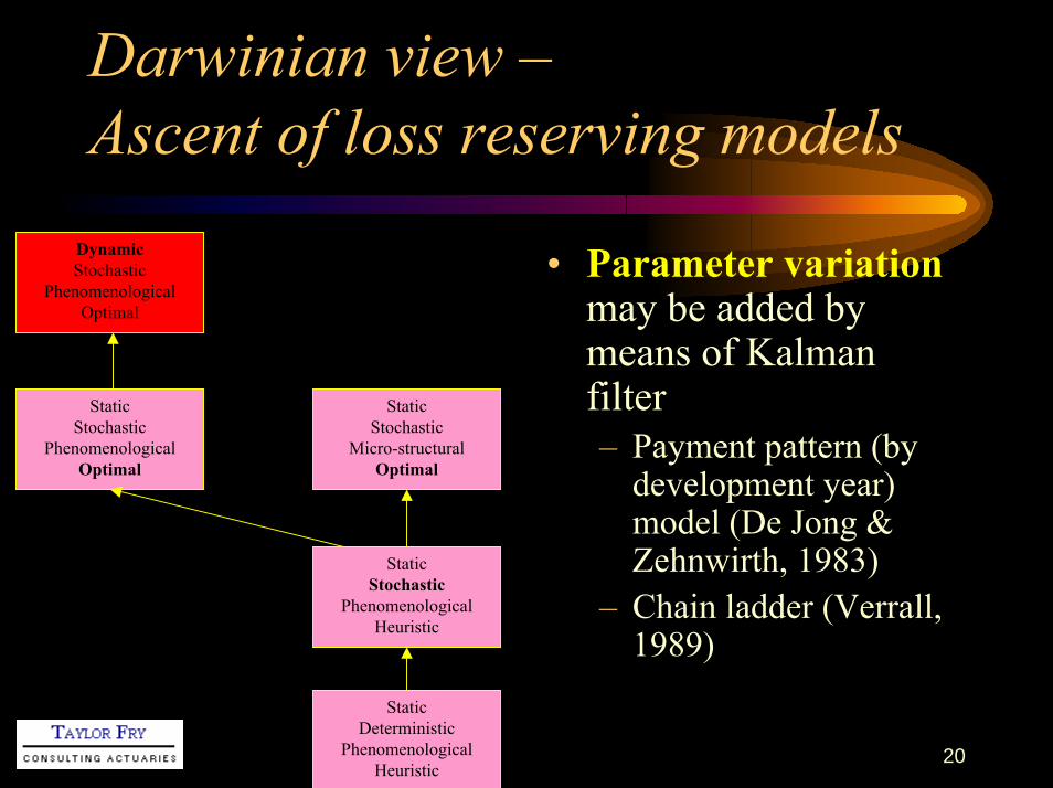
Darwinian view –Ascent of loss reserving models
• Parameter variation may be added by means of Kalman filter– Payment pattern (by
development year) model (De Jong & Zehnwirth, 1983)
– Chain ladder (Verrall, 1989)
StaticDeterministic
PhenomenologicalHeuristic
StaticStochastic
PhenomenologicalHeuristic
StaticStochastic
Micro-structuralOptimal
StaticStochastic
PhenomenologicalOptimal
DynamicStochastic
PhenomenologicalOptimal

21
Darwinian view –Ascent of loss reserving models
• Kalman filter may be bolted onto many stochastic models– though with some
shortcomings, to be discussed
StaticDeterministic
PhenomenologicalHeuristic
StaticStochastic
PhenomenologicalHeuristic
StaticStochastic
Micro-structuralOptimal
StaticStochastic
PhenomenologicalOptimal
DynamicStochastic
Micro-structuralOptimal
DynamicStochastic
PhenomenologicalOptimal

Adaptive loss reserving

23
Adaptive loss reserving
• By this we mean loss reserving based on dynamic models– Kalman filter is an example
• Kalman,1960 – engineering• Harrison & Stevens, 1976 – statistical• De Jong & Zehnwirth, 1983 - actuarial
– We wish to generalise this
24
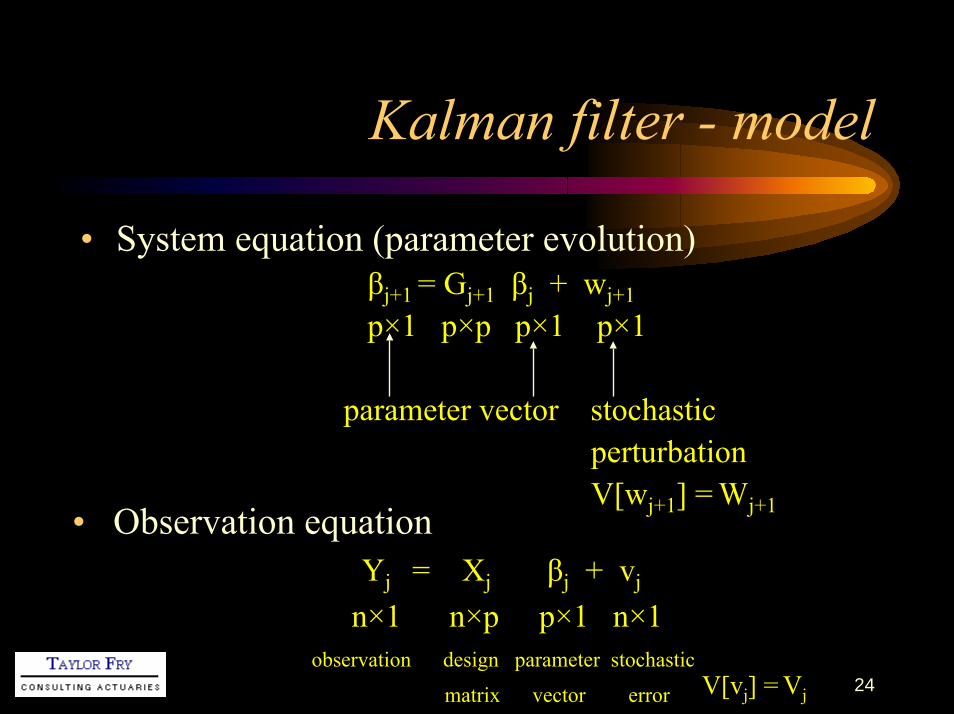
Kalman filter - model
• System equation (parameter evolution)βj+1 = Gj+1 βj + wj+1p×1 p×p p×1 p×1
parameter vector stochasticperturbation V[wj+1] = Wj+1• Observation equation
Yj = Xj βj + vj
n×1 n×p p×1 n×1observation design parameter stochastic
matrix vector error V[vj] = Vj
25
Kalman filter - operation
• Updates parameter estimates iteratively over time
• Each iteration introduces additional information from a single epoch

26
Notation
• For any quantity Yj depending on epoch j, let
Yj|k = estimate of Yj on the basis of information up to and including epoch k
Γj|k = V[βj|k] = parameter estimation error
27
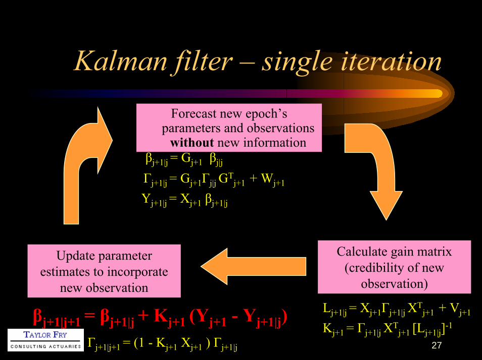
Kalman filter – single iterationForecast new epoch’s
parameters and observations without new information
βj+1|j = Gj+1 βj|j
Γj+1|j = Gj+1Γj|j GTj+1 + Wj+1
Yj+1|j = Xj+1 βj+1|j
Calculate gain matrix (credibility of new
observation)
Update parameter estimates to incorporate
new observationLj+1|j = Xj+1Γj+1|j XT
j+1 + Vj+1
Kj+1 = Γj+1|j XTj+1 [Lj+1|j]-1
βj+1|j+1 = βj+1|j + Kj+1 (Yj+1 - Yj+1|j)Γj+1|j+1 = (1 - Kj+1 Xj+1 ) Γj+1|j
28
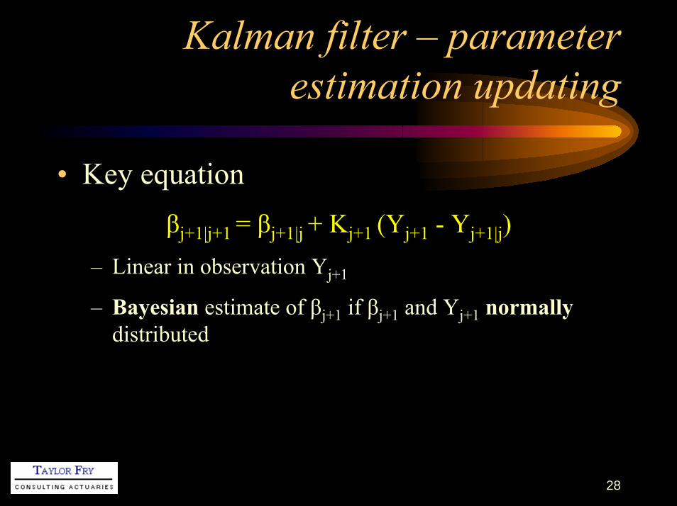
Kalman filter – parameter estimation updating
• Key equationβj+1|j+1 = βj+1|j + Kj+1 (Yj+1 - Yj+1|j)
– Linear in observation Yj+1
– Bayesian estimate of βj+1 if βj+1 and Yj+1 normally distributed
29
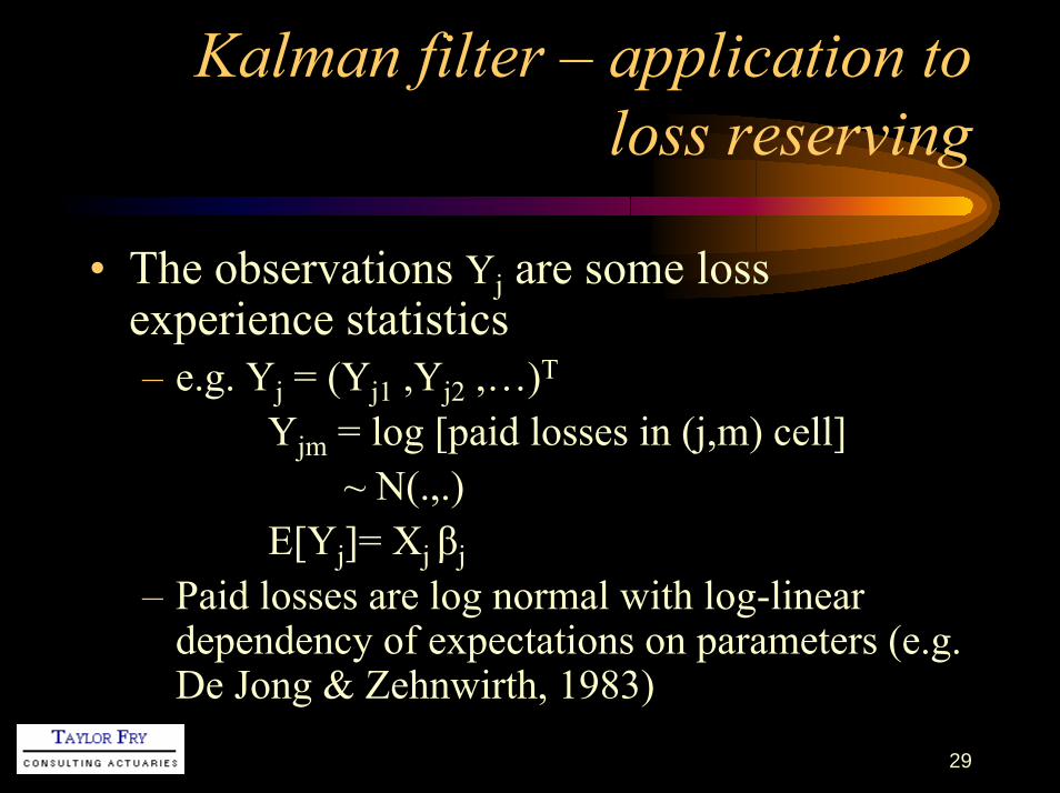
Kalman filter – application to loss reserving
• The observations Yj are some loss experience statistics– e.g. Yj = (Yj1 ,Yj2 ,…)T
Yjm = log [paid losses in (j,m) cell]~ N(.,.)
E[Yj]= Xj βj– Paid losses are log normal with log-linear
dependency of expectations on parameters (e.g. De Jong & Zehnwirth, 1983)

30
Kalman filter – loss modelling difficulties
• Model error structureYj ~ N(.,.)
• May not be suitable for claim count data• Usually requires that Yj be some
transformation of loss statistics (e.g. log)• Inversion of transformation introduces need
for bias correction• Can be awkward

31
Dynamic models with non-normal errors
• Kalman model– System equationβj+1 = Gj+1 βj + wj+1
– Observation equationYj = Xj βj + vj
vj ~ N(0,Vj)
• Alternative model– System equationβj+1 = Gj+1 βj + wj+1
– Observation equationYj satisfies GLM with
linear predictor Xj βjYj from exponential dispersion
family (EDF)
E[Yj] = h-1(Xj βj)
• How should this be filtered?

32
Filtering as regression
• Kalman estimation equationβj+1|j+1 = βj+1|j + Kj+1 (Yj+1 - Yj+1|j)
– Linear in prior estimate βj+1|j and observation Yj+1
– View as regression of vector [YTj+1, βT
j+1|j]T on βj+1
Yj+1 = Xj+1 βj+1 + vj+1 , V vj+1 = Vj+1 0βj+1|j 1 uj+1 uj+1 0 Γj+1|j

33
EDF filter
Kalman filterIdentity Normal
Yj+1 = h-1 Xj+1 βj+1 + vj+1 , V vj+1 = Vj+1 0βj+1|j 1 uj+1 uj+1 0 Γj+1|j
generally notdiagonal
Non-identity EDF
EDF filter
34
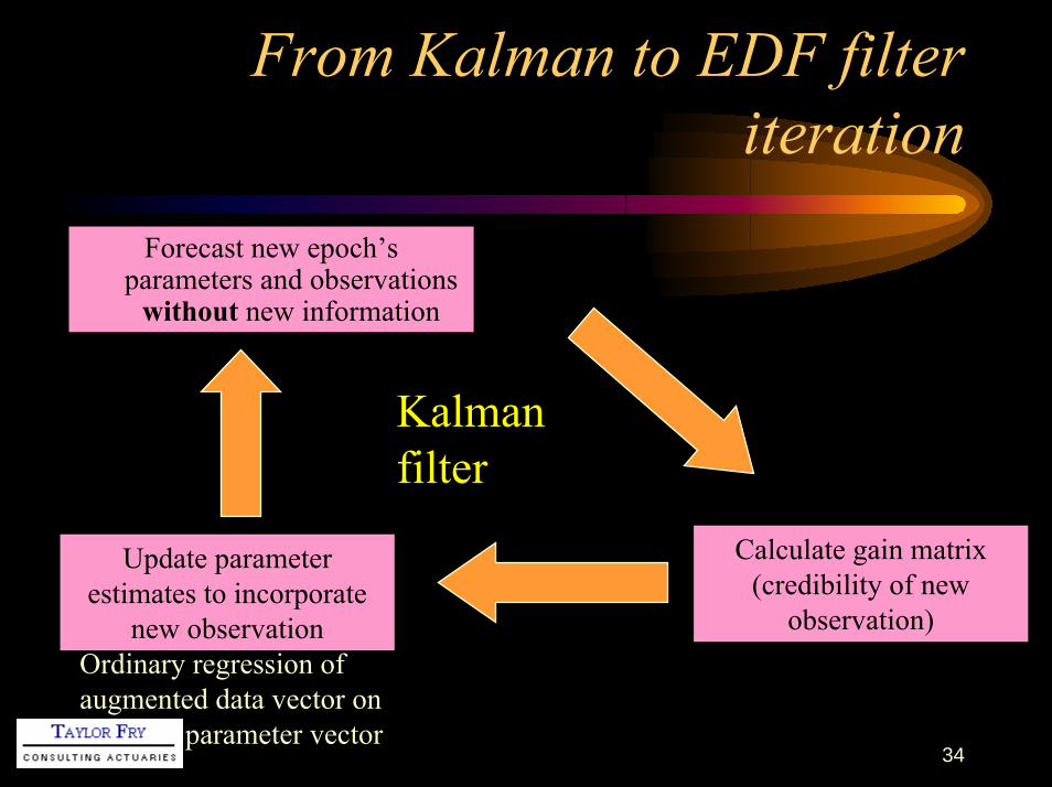
From Kalman to EDF filter iteration
Forecast new epoch’s parameters and observations
without new information
Kalman filter
Calculate gain matrix (credibility of new
observation)
Update parameter estimates to incorporate
new observationOrdinary regression of augmented data vector on
parameter vector

35
From Kalman to EDF filter iteration
Forecast new epoch’s parameters and observations
without new information
EDF filter
Calculate gain matrix (credibility of new
observation)
Update parameter estimates to incorporate
new observationGLM regression of augmented data vector on
parameter vector

36
From Kalman to EDF filter iteration
For use of GLM regression softwareForecast new epoch’s
parameters and observations without new information Linear transformation
of estimated parameter vector to diagonal covariance matrixEDF
filter
Calculate gain matrix (credibility of new
observation)
Update parameter estimates to incorporate
new observationGLM regression of augmented data vector on
parameter vector

37
From Kalman to EDF filter iteration
Forecast new epoch’s parameters and observations
without new information
Calculate gain matrix (credibility of new
observation)
Update parameter estimates to incorporate
new observationGLM regression of augmented data vector on
parameter vector
EDF filter
Linear transformation of estimated parameter
vector to diagonal covariance matrix
For use of GLM regression software
Software performs this step

38
EDF filter – theoretical justification
• “Approximate” Bayes estimator– Refer
• Jewell (AB 1974)• Nelder & Verrall (AB 1997)• Landsman & Makov (SAJ 1998)
for the (exact) 1-dimensional case• Stochastic approximation
– refer Landsman & Makov (SAJ 1999, 2003) for the 1-dimensional case

Numerical examples

40
Example 1 – Filtering rows of Payments per claim incurred
• Workers compensation portfolio– Claim payments dominated by weekly
compensation benefits– Half-yearly data– Consider triangle of payments (inflation
corrected) per claim incurred in the accident half-year

41
Example 1 – Filtering rows of Payments per claim incurred
• Gradual changes in the pattern of payments are evident from one accident half-year to another

42
Example 1 – Filtering rows of Payments per claim incurred
PPCI by accident half-year
0
500
1000
1500
2000
2500
0 1 2 3 4 5 6 7 8 9 10 11 12 13 14 15 16 17 18 19 20 21 22 23 24 25
development half-year
PPC
I
89H2 90H1 94H2 98H2

43
Example 1 – Filtering rows of Payments per claim incurred
• Model these changes with EDF filter– Log link– Gamma error– Observation vectors = Rows of triangle

44
Example 1 – Filtering rows of Payments per claim incurred
• Initiation of filter
0
500
1000
1500
2000
2500
1 2 3 4 5 6 7 8 9 10 11 12 13 14 15 16 17 18 19 20 21 22 23 24 25 26
development half-year
PPC
I
89H2 data 89H2 fitted

45
Example 1 – Filtering rows of Payments per claim incurred
• Adding the next row of data
0
500
1000
1500
2000
2500
1 2 3 4 5 6 7 8 9 10 11 12 13 14 15 16 17 18 19 20 21 22 23 24 25 26
development half-year
PPC
I
89H2 data 89H2 fitted 90H1 data

46
Example 1 – Filtering rows of Payments per claim incurred
• 90H1 posterior (fitted curve) developed from prior (89H2 fitted curve) and data
0
500
1000
1500
2000
2500
0 1 2 3 4 5 6 7 8 9 10 11 12 13 14 15 16 17 18 19 20 21 22 23 24 25
development half-year
PPC
I
89H2 fitted 90H1 data 90H1 fitted
47
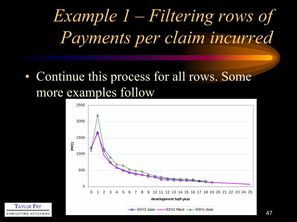
Example 1 – Filtering rows of Payments per claim incurred
• Continue this process for all rows. Some more examples follow
0
500
1000
1500
2000
2500
0 1 2 3 4 5 6 7 8 9 10 11 12 13 14 15 16 17 18 19 20 21 22 23 24 25
development half-year
PPC
I
92H2 data 92H2 fitted 93H1 data

48
Example 1 – Filtering rows of Payments per claim incurred
0
500
1000
1500
2000
2500
0 1 2 3 4 5 6 7 8 9 10 11 12 13 14 15 16 17 18 19 20 21 22 23 24 25
development half-year
PPC
I
92H2 fitted 93H1 data 93H1 fitted

49
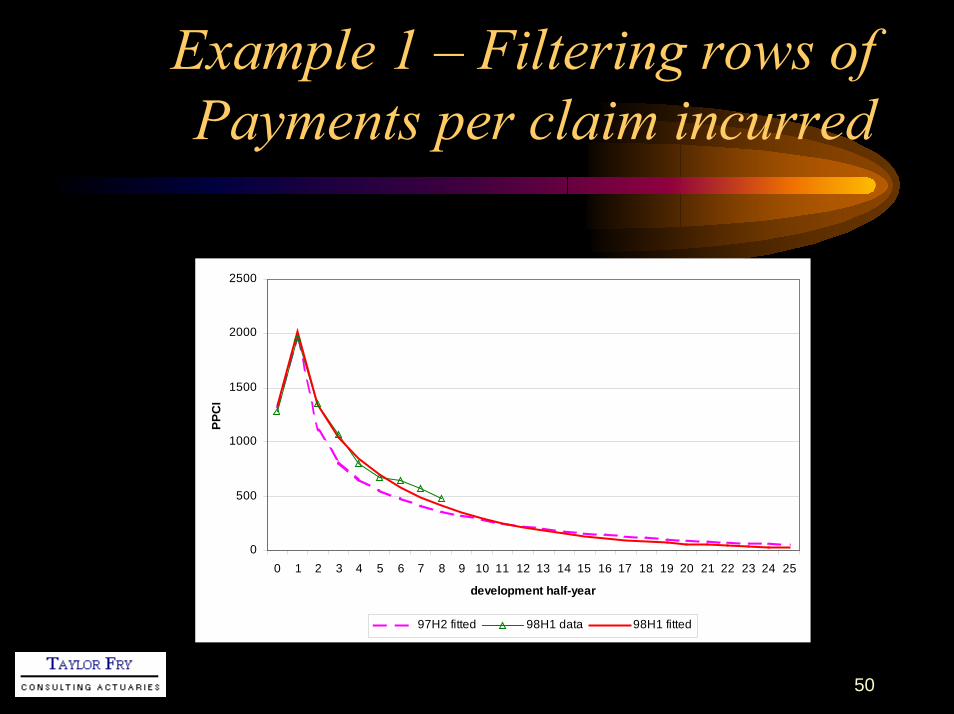
Example 1 – Filtering rows of Payments per claim incurred
0
500
1000
1500
2000
2500
0 1 2 3 4 5 6 7 8 9 10 11 12 13 14 15 16 17 18 19 20 21 22 23 24 25
development half-year
PPC
I
97H2 data 97H2 fitted 98H1 data
50
Example 1 – Filtering rows of Payments per claim incurred
0
500
1000
1500
2000
2500
0 1 2 3 4 5 6 7 8 9 10 11 12 13 14 15 16 17 18 19 20 21 22 23 24 25
development half-year
PPC
I
97H2 fitted 98H1 data 98H1 fitted

51
Example 2 – Filtering diagonals of claim closure rates
• Motor Bodily Injury portfolio– From Taylor (2000)– Annual data– Consider triangle of claim closure rates:
Number of claims closed in cellNumber open at start + 1/3 × number newly reported in cell

52
Example 2 – Filtering diagonals of claim closure rates
• Claim closure rates subject to upward or downward shocks from time to time
1 2 3 4 5 6 7 8 9 10 11 12 13 >13
De v e lo p m e n t ye a r
0%
10%
20%
30%
40%
50%
60%
70%
Clo
sure
rate
Exp yrs 1 9 9 1 -9 2 Exp yrs 1 9 8 9 -9 0 Exp yrs 1 9 8 4 -8 5
Claim closure rates

53
Example 2 – Filtering diagonals of claim closure rates
• Model these changes with EDF filter– Identity link– Normal error (Kalman filter)
• To be changed to binomial or quasi-Poisson
– Observation vectors = Diagonals of triangle
54
Example 2 – Filtering diagonals of claim closure rates
i = accident year (row)j = development year (column)k = i+j = experience year (diagonal)C(j,k) = Claim closure rate

55
Example 2 – form of model
C(j,k) ~ N(µ(j,k), σ2(j,k))µ(j,k) = exp [f(j) + g(k)]
Pattern of closure Upward or downwardrate over shock in
development year experience year
g(k) ~ N(0,.)
unrelated to g(k-1), g(k-2), etc.

56
Example 2 – Filtering diagonals of claim closure rates
• Data plotted by finalisation year– each graph will relate to a number of accident
years– Fitted points share common experience year
shocks but have different development year curves, dependent on accident year

57
Example 2 – Filtering diagonals of claim closure rates
• 1981 fitted becomes prior for 1982 data
0.0
0.1
0.2
0.3
0.4
0.5
0.6
0.7
0.8
1 2 3 4 5 6 7 8 9 10 11 12 13 14 15 16 17
Development year
Cla
im c
losu
re ra
te
1981 data 1981 fitted 1982 data

58
Example 2 – Filtering diagonals of claim closure rates
Leading to
0.0
0.1
0.2
0.3
0.4
0.5
0.6
0.7
0.8
1 2 3 4 5 6 7 8 9 10 11 12 13 14 15 16 17
Development year
Cla
im c
losu
re ra
te
1981 fitted 1982 data 1982 fitted

59
Example 2 – Filtering diagonals of claim closure rates
Some more examples:
0.0
0.1
0.2
0.3
0.4
0.5
0.6
0.7
0.8
1 2 3 4 5 6 7 8 9 10 11 12 13 14 15 16 17
Development year
Cla
im c
losu
re ra
te
1990 data 1990 fitted 1991 data

60
Example 2 – Filtering diagonals of claim closure rates
0.0
0.1
0.2
0.3
0.4
0.5
0.6
0.7
0.8
1 2 3 4 5 6 7 8 9 10 11 12 13 14 15 16 17
Development year
Cla
im c
losu
re ra
te
1990 fitted 1991 data 1991 fitted

61
Example 2 – Filtering diagonals of claim closure rates
0.0
0.1
0.2
0.3
0.4
0.5
0.6
0.7
0.8
1 2 3 4 5 6 7 8 9 10 11 12 13 14 15 16 17
Development year
Cla
im c
losu
re ra
te
1991 data 1991 fitted 1992 data
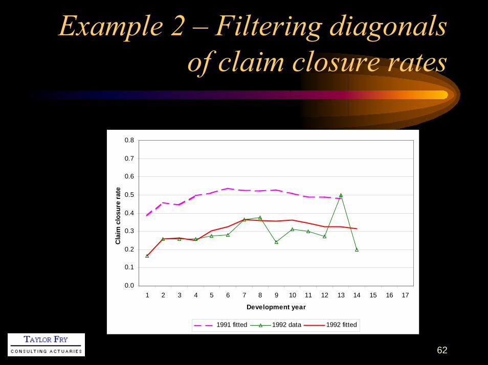
62
Example 2 – Filtering diagonals of claim closure rates
0.0
0.1
0.2
0.3
0.4
0.5
0.6
0.7
0.8
1 2 3 4 5 6 7 8 9 10 11 12 13 14 15 16 17
Development year
Cla
im c
losu
re ra
te
1991 fitted 1992 data 1992 fitted

Future loss reserving

64
The claims experience triangle
j
i
C(i,j)
• Nearly all loss reserving methodology related to the triangle
• But this is only a convenient summary of much more extensive data– Driven by the computational
needs of a bygone era• Why not develop methodology
geared to unit record claim data?
65
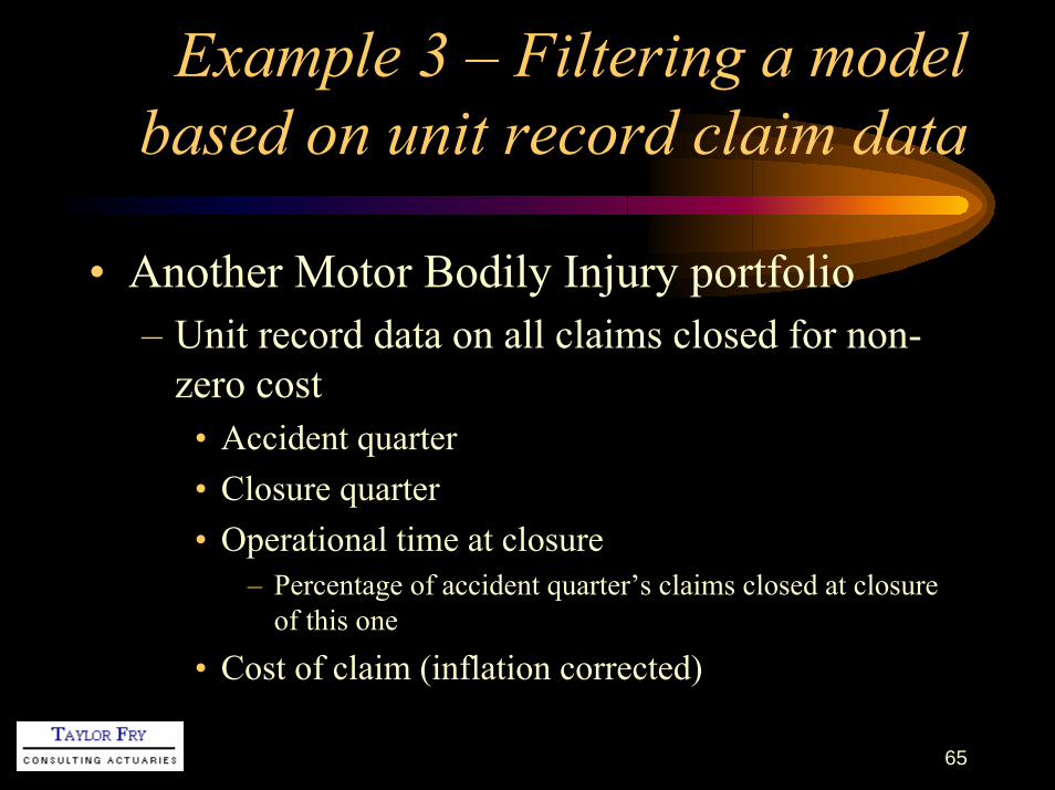
Example 3 – Filtering a model based on unit record claim data
• Another Motor Bodily Injury portfolio– Unit record data on all claims closed for non-
zero cost• Accident quarter• Closure quarter• Operational time at closure
– Percentage of accident quarter’s claims closed at closure of this one
• Cost of claim (inflation corrected)

66
Example 3 – Filtering a model based on unit record claim data
• Form of modeli = accident quarter (row)j = development quarter (column)k = i+j = experience quarter (diagonal)t = operational time at claim closureC(t,i,k) = Cost of an individual claim (inflation
corrected)•Good illustrative example because
–Introduces a number of complexities–Does so in a mathematically simple manner–Does so dynamically
67
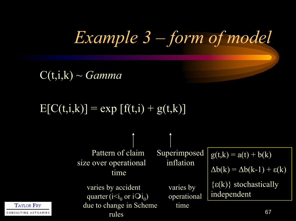
Example 3 – form of model
C(t,i,k) ~ Gamma
E[C(t,i,k)] = exp [f(t,i) + g(t,k)]
Pattern of claim Superimposedsize over operational inflation
time
g(t,k) = a(t) + b(k)
∆b(k) = ∆b(k-1) + ε(k)
{ε(k)} stochastically independent
varies by accident varies byquarter (i<i0 or i i0) operational
due to change in Scheme timerules
68
Example 3 – filter diagonals of closed claim sizes
• Diagonals are as usual– Quarters of claim closure
• BUT each new diagonal consists of vector of individual sizes of closed claims

69
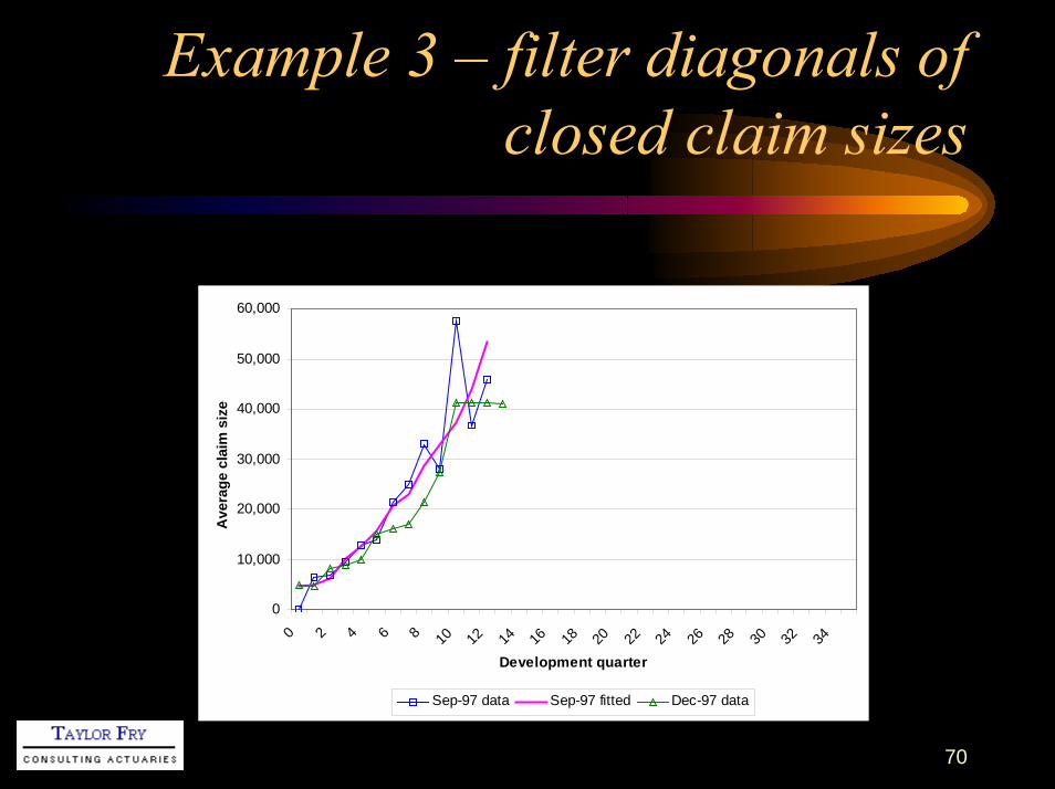
Example 3 – filter diagonals of closed claim sizes
• Once again, graphs show fitted points by finalisation quarter– Average value in each development quarter
shown– Each point shares superimposed inflation
parameters• superimposed inflation varies over operational time
– Each point has individual operational time parameters dependent on accident quarter
70
Example 3 – filter diagonals of closed claim sizes
0
10,000
20,000
30,000
40,000
50,000
60,000
0 2 4 6 8 10 12 14 16 18 20 22 24 26 28 30 32 34
Development quarter
Ave
rage
cla
im s
ize
Sep-97 data Sep-97 fitted Dec-97 data

71
Example 3 – filter diagonals of closed claim sizes
0
10,000
20,000
30,000
40,000
50,000
60,000
0 2 4 6 8 10 12 14 16 18 20 22 24 26 28 30 32 34
Development quarter
Ave
rage
cla
im s
ize
Sep-97 fitted Dec-97 data Dec-97 fitted

72
Example 3 – filter diagonals of closed claim sizes
0
20,000
40,000
60,000
80,000
100,000
120,000
140,000
160,000
180,000
200,000
0 2 4 6 8 10 12 14 16 18 20 22 24 26 28 30 32 34
Development quarter
Ave
rage
cla
im s
ize
Sep-00 data Sep-00 fitted Dec-00 data

73
Example 3 – filter diagonals of closed claim sizes
0
20,000
40,000
60,000
80,000
100,000
120,000
140,000
160,000
180,000
200,000
0 2 4 6 8 10 12 14 16 18 20 22 24 26 28 30 32 34
Development quarter
Ave
rage
cla
im s
ize
Sep-00 fitted Dec-00 data Dec-00 fitted
74
Example 3 – filter diagonals of closed claim sizes
• Interesting to look at trends in the superimposed inflation (SI) parameters
• Shape of SI is piecewise linear in operational time
• Other analysis has suggested an increase in SI at the December 2000 quarter and a further increase from March 2002
• Is this recognised by the filter?

75
Example 3 – filter diagonals of closed claim sizes
-10%
-8%
-6%
-4%
-2%
0%
2%
4%
6%
8%
10%
0 10 20 30 40 50 60 70 80 90 100
operational time
annu
alis
ed S
I
Jun-00 Sep-00 Dec-00
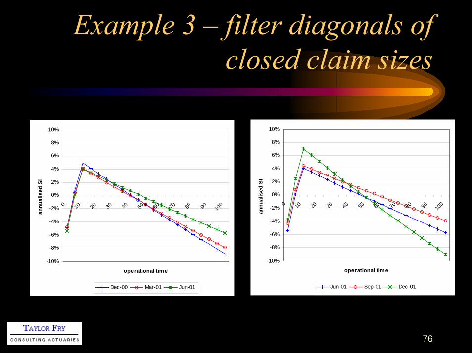
• Graph shows SI by operational time for 3 successive development quarters
• Increase at Dec00• Upwards trend
continues
76
Example 3 – filter diagonals of closed claim sizes
-10%
-8%
-6%
-4%
-2%
0%
2%
4%
6%
8%
10%
0 10 20 30 40 50 60 70 80 90 100
operational time
annu
alis
ed S
I
Jun-01 Sep-01 Dec-01
-10%
-8%
-6%
-4%
-2%
0%
2%
4%
6%
8%
10%
0 10 20 30 40 50 60 70 80 90 100
operational time
annu
alis
ed S
I
Dec-00 Mar-01 Jun-01

77
Example 3 – filter diagonals of closed claim sizes
• We have observed a further significant increase in SI from Mar02
• Again this is reflected by the filter
-10%
-8%
-6%
-4%
-2%
0%
2%
4%
6%
8%
10%
0 10 20 30 40 50 60 70 80 90 100
operational time
annu
alis
ed S
I
Dec-01 Mar-02 Jun-02

78
Example 3 – filter diagonals of closed claim sizes
• Has the trend in SI stopped at Mar03?
-10%
-8%
-6%
-4%
-2%
0%
2%
4%
6%
8%
10%
0 10 20 30 40 50 60 70 80 90 100
operational time
annu
alis
ed S
I
Mar-02 Jun-02 Sep-02
-10%
-8%
-6%
-4%
-2%
0%
2%
4%
6%
8%
10%
0 10 20 30 40 50 60 70 80 90 100
operational time
annu
alis
ed S
I
Sep-02 Dec-02 Mar-03
Related Documents