Longitudinal Cross-Gender Factorial Invariance of the ...selfdeterminationtheory.org/SDT/documents/2006_GrouzetOtis... · differences in motivation between females and ... thus estimated

Longitudinal Cross-GenderFactorial Invariance of the Academic

Motivation Scale

Frederick M. E. Grouzet, Nancy Otis, and Luc G. PelletierUniversity of Ottawa

This study examined the measurement and latent construct invariance of the Aca-demic Motivation Scale (Vallerand, Blais, Brière, & Pelletier, 1989; Vallerand et al.,1992, 1993) across both gender and time. An integrative analytical strategy was usedto assess in one set of nested models both longitudinal and cross-gender invariance,and “interactional” and “simple” tests of invariance (e.g., cross-gender invarianceacross waves) were conducted. Results from a sample of 643 students (322 boys and321 girls) across a 3-year time span showed good longitudinal cross-gender factorialinvariance with different degrees of invariance depending on the sample, the educa-tional level, or both. Implications for the validity of the Academic Motivation Scale,as well as for research on factorial invariance, are discussed.

Over the past 30 years, research on student motivation has flourished and remains acontemporary and important topic in education and psychology. In education, mo-tivation is primarily studied in relation to school performance, as well as to thechoices students make about which academic activities to engage in, their persis-tence in continuing these activities, and the degree of effort they expend. Exploringthe why of students’ behavior, several motivation theorists have made a distinctionbetween intrinsic and extrinsic motivations (e.g., Deci, Vallerand, Pelletier, &Ryan, 1991; Harter, 1981). Intrinsic motivation generally refers to performing anactivity as an end in and of itself—for the pleasure and satisfaction derived fromthis participation (e.g., Deci, 1975). On the other hand, extrinsic motivation refersto engaging in an activity as a means to an end; that is, to obtain something positiveor to avoid something negative external to the activity (Deci, 1975). However,

STRUCTURAL EQUATION MODELING, 13(1), 73–98Copyright © 2006, Lawrence Erlbaum Associates, Inc.

Correspondence should be addressed to Frederick M.E. Grouzet, Educational & CounselingPsychology, McGill University, 3700 McTavish, Montreal, Quebec H3A 1Y2, Canada. E-mail:[email protected]

some researchers have proposed a multidimensional view of extrinsic motivation.For instance, according to self-determination theory (Deci & Ryan, 1985, 2000),there are four types of extrinsic motivation: External and introjected regulations re-fer to conducting an activity due to an external and internal (respectively) sense ofobligation to obtain something positive or to avoid something negative beyond theactivity itself (e.g., Deci & Ryan, 1985), whereas identified and integrated regula-tions refer to engaging in an activity by personal choice (more or less integrated inthe self; see e.g., Deci & Ryan, 1985). These four types of regulatory processes fallalong a self-determination continuum from the least to most self-determined moti-vation, that is external, introjected, identified, and integrated regulation. Intrinsicmotivation is defined as the prototype of self-determined activity and thus is placedat the self-determined pole of this continuum, and amotivation (i.e., the relative ab-sence of motivation) is placed at the opposite pole (for a complete review ofself-determination theory see Deci & Ryan, 2000).

To study intrinsic and extrinsic motivation according to self-determination the-ory’s multidimensional perspective, a great deal of effort has been made to createand validate multiconstruct scales. Along these lines, Vallerand and his colleagueshave developed the Academic Motivation Scale (AMS; Vallerand et al., 1992,1993; its French version is the “Échelle de Motivation en Éducation” or ÉMÉ;Vallerand, Blais, Brière, & Pelletier, 1989). The AMS is one of the most frequentlyused scales to measure intrinsic and extrinsic academic motivation. The AMS hasbeen integrated in empirical models which incorporate both determinants (e.g.,school environment, parental engagement, professors’ behaviors) and conse-quences (e.g., dropout, school performance, interest) of academic motivation (seee.g., Guay & Vallerand, 1997; Pelletier, Séguin-Lévesque, & Legault, 2002;Vallerand, Fortier, & Guay, 1997), providing support for its construct and predic-tive validity. The AMS has also been validated with various populations, withmales and females, with English- and French-speaking students, across variousgeographic areas (e.g., Canada, United States, France), and from senior highschool to university level. However, the AMS has never been tested for invarianceacross different groups or across time. Considering that a few studies have reporteddifferences in motivation between females and males, the examination ofcross-gender invariance would allow the interpretation of whether observed differ-ences are at the construct level (i.e., true motivational differences) or at the mea-surement level (i.e., differences in scaling). Furthermore, support for the AMS’slongitudinal invariance would enable researchers to further test hypotheses aboutthe development (i.e., change) in students’ motivation across education levels.

Confirmatory factor analysis (CFA) framework is ideally suited for testingwhether scores measure “the correct something” (rather than “nothing”; Thomp-son, 2003) and whether the meaning of this “something” is equivalent across sam-ples or times. Likewise, a recent review of literature by Vandenberg and Lance(2000) indicated that interest in examining factorial invariance (FI) from a CFA

74 GROUZET, OTIS, PELLETIER

perspective is pivotal and extensive. In fact, the authors detected more than 14 dif-ferent recommended procedures for testing FI. This lack of consensus indicatesthat FI procedures are still in development. Furthermore, Vandenberg and Lancefound 67 other articles in which other researchers used various approaches to testFI, mostly across samples (i.e., gender, cultures, etc.) but also across time. How-ever, no study has examined FI across both samples and time in only one group ofnested models. Therefore, testing FI of the AMS across gender and time providesan interesting challenge for FI research. Moreover, this challenge is ever greaterdue to the multidimensional nature of the AMS.

The purpose of the study was to examine further aspects of validity of the AMSwith elementary and junior high-school students (i.e., from 8th to 10th grade) us-ing an integrated structural equation modeling strategy. In particular, the study si-multaneously examined both longitudinal and cross-gender FI of the AMS with ananalytical strategy, using the mean and covariance structures (MACS) technique(e.g., T.D. Little, 1997), and other new approaches proposed by structural equationmodeling theorists working on FI (see Vandenberg & Lance, 2000). Finally, thestudy hoped to show the generalizability of this analytical strategy for testing bothinterindividual (i.e., across samples) and intraindividual (e.g., across times) FIcombined.

METHODS

Participants and Procedure

The data analyzed in this study came from a large longitudinal project conductedin an Ontario Catholic French-speaking school board (Pelletier, 2004). Over a pe-riod of 3 years (from 2001 to 2003), 322 boys and 321 girls in 8th, 9th, and 10thgrades completed the French version of the AMS (Vallerand et al., 1989). Meanages for 8th, 9th, and 10th grades were 13-, 14-, and 15-years-old, respectively.The questionnaire was answered during regular class hours. For the 8th graders,questions were read aloud to ascertain a good understanding of the questions.Ninth and 10th graders answered the questions independently.

Instrument

The AMS included five subscales assessing intrinsic motivation (IM), identifiedregulation (ID), introjected regulation (IJ), external regulation (ER), andamotivation (AM) with 4 items each, totaling 20 items. Students were asked “Whyare you going to school?” and the response choices for each item were rated on a5-point Likert-type scale from 0 (does not correspond at all) to 4 (corresponds ex-actly). The items can be found in Vallerand et al. (1989, 1992).

LONGITUDINAL CROSS-GENDER INVARIANCE 75

Missing Data

In most longitudinal studies, missing data and attrition are frequent. This study wasno exception. More than 30 different missing patterns were detected in each boy andgirl sample.Amongthem, tworelevantattritionpatternswerefoundin9th-gradeand10th-grade waves. More specifically, 80 girls and 76 boys were absent from the9th-grade wave, and 62 girls and 72 boys were absent from the 10th-grade wave. Al-though the presence of these two missing patterns suggests using multisample tech-niques for handling missing data (e.g., Muthén, Kaplan, & Hollis, 1987), the maxi-mum likelihood estimate of missing data was used because of the presence of otherpatterns and also because a multisample approach (in addition to the gender subdivi-sion) may require a more complex design. Results from Kim and Bentler’s (2002)test of homogeneity of means and covariances revealed that the missing completelyat random assumption for both means and covariances was not rejected for the boysample but was rejected for the girl sample. For the purpose of this study, it was as-sumed that the data was missing at random (R.J.A. Little & Rubin, 1987). Therefore,the study used Jamshidian and Bentler’s (1999) EM-type (Expected Maximization)missingdataprocedures formultiplesamples to replace them.Thenacompletesetofdata was worked on.

Analyzing Longitudinal Cross-Sample Invariance

The following sections describe the analytical strategy that was used in the study.To provide useful information for interested researchers each aspect of the analy-ses is detailed. Although the analyses were applied to the study data, further appli-cations to other data are easily possible.

Parameters in MACS framework. The MACS approach, which was pro-posed by T.D. Little (1997), distinguishes measurement and latent construct param-eters. Measurement parameters correspond to pattern loadings (λ), intercepts (τ),and measurement errors (θε). In this study, there were five subscales (i.e., intrinsicmotivation, identified regulation, introjected regulation, external regulation, andamotivation) with 4 items each, totaling 20 items. Girls and boys responded to these20 items each year for 3 years. Thus, this model involved 20(items) × 2(girls vs.boys) × 3(waves) = 120 loadings, as well as 120 intercepts, and 120 errors.

Latent construct parameters. These are standard deviations (σ), correla-tions (ψ),1 and means (α). In this study, there were 5(motivational constructs) ×2(girls vs. boys) × 3(waves) = 30 latent standard deviations, as well as 30 latent


1Latent standard deviation is estimated via a regression path between the latent construct (for whichvariance is fixed to zero) and a phantom variable (for which variance is fixed to 1). Latent correlation isthus estimated by a covariance parameter between two phantom variables. For more information, thereader is referred to Little (1997); see also McArdle & Cattell (1994).

means. There were three types of correlations. First, there were the interrelationsamong the five latent motivational constructs (i.e., intrinsic motivation, identifiedregulation, introjected regulation, external regulation, and amotivation). The totalwas 10(interrelations among motivational constructs) × 2(girls vs. boys) ×3(waves) = 60 correlations. Second, for each motivational construct one can assesslongitudinal stability by estimating correlations among latent factors across waves.Three waves means there were three separate stability coefficients (i.e., from 8th to9th grade, from 9th to 10th grade, and from 8th to 10th grade), totaling 3 × 5(moti-vational constructs) × 2(girls vs. boys) = 30 correlations. A third type of correla-tion involved relations among different motivational constructs across waves (e.g.,intrinsic motivation in 8th grade with external regulation in 9th grade). Becausethis was not the scope of this study, theoretical meaning was not associated withthis last group of correlations.

Finally, in both girl and boy groups, adjacent cross-time correlations amongmeasurement errors were estimated, totaling 20(items) × 2(adjacent pairs of er-rors; i.e., from 8th to 9th grade and from 9th to 10th grade) = 40 error correlations.

Standardization and identification. When estimating a one-sample CFAmodel, there are two ways to standardize a latent construct (i.e., reach scale identi-fication). A direct way is to fix the variance (i.e., η = 1, or the standard deviation [σ= 1] estimated through the path regression—see footnote 1) and the latent mean(i.e., α = 0) of the latent constructs. An indirect way is to fix the pattern loading(i.e., λy = 1) and the intercept (i.e., τy = 0) of one selected item. However, when esti-mating a multisample CFA model, problems may arise when the entity (especiallyη and λy,) used for standardization (i.e., fixed to unity across samples) is not actu-ally invariant across samples (see e.g., Cheung & Rensvold, 1999; Reise,Widaman, & Pugh, 1993). Therefore, various authors have proposed various stan-dardization procedures, which are more or less equivalent for a “global test” (i.e.,full invariance test) but may be inadequate for a partial invariance test (see e.g.,Cheung & Rensvold, 1999; Reise et al., 1993).

In this study, a method of standardization adapted from Reise et al.’s (1993) rec-ommendation (see also Cheung & Rensvold, 1999; Steenkamp & Baumgartner,1998) was used. First, the study fixed the five latent standard deviations (i.e., pathregressions), as well as the five latent means of the five motivational constructs of areferent “group” (i.e., girls in eighth grade: IM8th-G, ID8th-G, IJ8th-G, EX8th-G, andAM8th-G).2 Second, the study constrained the pattern loadings (λ1) and the inter-


2MACS(andmultigroupCFA)must selectonesampleasa referent. In this study,girlswerearbitrarilyselected. In a longitudinal model, the choice of a reference point is less arbitrary and corresponds more of-ten to the first wave (i.e., 8th grade). Therefore, the five motivational constructs associated with the8th-grade-girl “group” were the reference points for the corresponding motivational constructs associ-atedwith the9th-grade-girl,10th-grade-girl,8th-grade-boy,9th-grade-boy,and10th-grade-boygroups.

cepts (τ1) of the first item of each motivational construct to be equal across samplesand waves. All other measurement and latent construct parameters were freely es-timated. This model was the basic model.

Testing invariance with nested sequences of models. The FI test wasthen conducted as a nested-model comparison between the basic model and one inwhich specific parameters were constrained to be equal across samples, waves, orboth. According to T.D. Little (1997), measurement and latent construct invariancewere distinguished. In general, researchers distinguish four levels of measurementinvariance (MI) corresponding to four nested models, as follows (from less to moreconstrained): (a) Configural invariance (Thurstone, 1947) is tested through the ba-sic model (or Mbasic) that estimates measurement and latent construct parameterswithout any constraints (excepted those specified previously); (b) Metricinvariance (Thurstone, 1947; Meredith’s, 1993, weak invariance) is tested throughmodels in which pattern factor loadings are constrained to be equal across samplesand waves—these metric models (Mmetric) are nested in the Mbasic models; (c) Sca-lar invariance (i.e., Meredith’s, 1993, strong invariance) is tested through modelsin which pattern factor loadings and intercepts are constrained to be equal acrosssamples and waves—these scalar models (Mscalar) are nested in the Mmetric models;(d) Uniqueness invariance (i.e., Meredith’s, 1993, strict invariance) is testedthrough models where pattern factor loadings, intercepts, and items’ unique vari-ances are constrained to be equal across samples and waves. These uniquenessmodels (Muniqueness) are nested in the Mscalar models.

Similarly, tests of latent construct invariance (or difference/change) also in-volve nested models. For the three types of latent construct parameters (i.e., stan-dard deviation, correlation, and mean) there are three corresponding models thatare nested in specific measurement models or in each other: (a) Latent standard de-viation invariance is tested through models nested in the Mmetric models, and thuspattern factor loadings and latent standard deviations are constrained to be equalacross samples and waves; (b) Latent correlation invariance is tested through mod-els that are nested in the Mmetric models, and thus pattern factor loadings and corre-lation are constrained to be equal across samples and waves; (c) Latent meaninvariance is tested through models nested in the Mscalar models, and pattern factorloadings, intercepts, and latent mean are constrained to be equal across samplesand waves.

A 2(samples) × 3(waves) MACS design. Most of the cross-sample andlongitudinal FI hypotheses that have been tested in the literature were tested sepa-rately. In the study, both cross-gender and longitudinal FI in one set of MACSnested models were simultaneously tested. Testing FI through a 2 × 3 design im-plies numerous nested model in which equality constraints are imposed on mea-surement and latent construct parameters, across gender, across waves, or both.


Figure 1 illustrates a 2 × 3 design for FI (see details later). The first part (Figure 1a)represents FI pertaining covariance structure, whereas the second part (Figure 1b)includes invariance levels pertaining mean structure.

The 2 × 3 design for MI is illustrated in the Figure 1b. Each column (from A toC) represents a cross-gender-invariance level, from configural to metric to scalarinvariance, and corresponds to a model in which a set of cross-gender equality con-straints is imposed. Each row (from 1 to 3) represents a longitudinal-invariancelevel, from configural to metric to scalar invariance, and corresponds to a model inwhich a set of equality constraints is imposed across waves. Degree-of-freedomdifferences (∆df) are shown on the arrows from one model to another nestedmodel, which correspond to the number of constraints imposed on the nestedmodel. For example, Model 2A was built to test longitudinal metric invariance andtherefore the 30 loadings (i.e., 3 items × 5 motivational constructs × 2 samples) forthe 9th-grade wave, as well as the 30 loadings in the 10th-grade wave, were con-strained to be equal to those in the 8th-grade wave, corresponding to a gain (or dif-ference) of 60 dfs in comparison with the baseline model (Model 1A). However,because of the “interactional” nature of the present invariance test, there wereoverlaps in constraints and degrees of freedom were therefore adjusted. For in-stance, in Model 2B the same 60 longitudinal metric invariance constraints as men-tioned previously were imposed in association with 45 cross-gender metricinvariance constraints (i.e., 3 items × 5 motivational constructs × 3 waves). Be-cause there were 30 overlapped constraints, the difference or gain of degrees offreedom (in comparison with Model 1A) was 75 rather than 60 + 45 = 105. The ad-justment of the degrees of freedom can also be seen when one compares degree offreedom gains from Model 1B to Model 2B (∆df = 30) and from Model 1A toModel 2A (∆df = 60) or when one compares degree of freedom gains from Model2A to Model 2B (∆df = 15) and from Model 1A to Model 1B (∆df = 45). Finally, itis worth noting that ∆df between two nested models, which are not juxtaposed inthe figure (e.g., Model 2B and Model 3C), can be calculated by adding ∆dfs be-tween intermediate nested models (e.g., 45 + 30 = 75).

This 2 × 3 design for MI is particularly useful for testing “simple effect” hy-potheses of MI. For instance, it becomes possible to test longitudinal invariance forgirls and for boys, separately (i.e., longitudinal invariance across gender). Further-more, this approach allows for the testing of cross-gender invariance at three peri-ods of life (i.e., 8th, 9th, and 10th grade) separately (i.e., gender invariance acrosswaves). As well, with this integrated approach one can test new “interactional” hy-potheses of MI. For instance, it becomes possible to examine the impact ofcross-gender (non-) invariance on a test of longitudinal invariance and vice versa.

The 2 × 3 designs can be extended to include latent constructs, such as standarddeviation and correlation invariance (Figure 1a; column D and E; row 4 and 5) andmean invariance (Figure 1b; column F; row 6), respectively. Similarly, for MI, the2 × 3 designs for latent constructs may be useful for testing specific hypotheses.


80

FIGURE 1 A set of nested models for testing the longitudinal cross-gender measurement invariance of the Academic Motivation Scale, the invarianceof standard deviation and correlation among motivational constructs (1a) and invariance of the latent means (1b).

81

FIGURE 1 (Continued)

Estimation procedure and fit indexes. Maximum likelihood estimationprocedures were used with Satorra and Bentler’s (1988, 1994) scaling corrections,allowing for the calculation of the Satorra-Bentler (SB) scaled chi-square value(SBχ2).3 Two types of fit indexes were used: overall and comparative fit indexes(see Bollen, 1989). The overall fit indexes used in the study were the SBχ2 statistic,the SBχ2/df ratio (an acceptable cutoff value is 3.00), the robust comparative fit in-dex (CFI; Bentler, 1990), the standardized root mean square residual (SRMR;Bentler, 1995), and the adjusted root mean squared error of approximation(RMSEA) for nonnormal conditions (see Nevitt & Hancock, 2000; Steiger & Lind,1980). As recommended by Widaman and Thompson (2003), the CFI (i.e., an in-cremental fit index) was calculated with statistics from an “acceptable” independ-ence null model, which is nested in the Mscalar analyses.4 Values equal or superiorto .90 for the CFI are considered to indicate a good fit, superior to .95 remainingideal (Hu & Bentler, 1999).5 Similarly, SRMR values equal to or smaller than .08are considered acceptable (Hu & Bentler, 1999). Finally, values for RMSEA lessthan .08 are used as thresholds for not rejecting a model (Browne & Cudeck, 1992;see also Hu & Bentler, 1999).

In addition to these overall fit indexes, two types of CFIs were also used to sta-tistically evaluate the difference between two nested models (see Bollen, 1989).First, the study used the scaled difference chi-square test (∆SBχ2; Satorra, 2000;Satorra & Bentler, 2001). Although it is not usually reported, the ∆SBχ2/∆df ratioto compare model differences for comparative purposes was also used. Second, asrecommended by Cheung and Rensvold (2002), the study also examined thechanges in the CFIs (i.e., the difference in the CFIs between two nested models or∆CFIs) when invariance constraints were added. A value of ∆CFI smaller than orequal to –.010 indicates that the invariance hypothesis should not be rejected. Oneof the advantages of the ∆CFI over the ∆SBχ2 is that it is not as strongly affected bysample size and number of constraints. Moreover, although much is known aboutthe efficacy of SBχ2 and ∆SBχ2, no research (to the best of our knowledge) hasevaluated such statistics for mean structures. Therefore, although the study exam-ined scalar invariance tests, the preferred focus was on overall indexes as well as∆CFI.


3The Satorra-Bentler rescaled estimation has been chosen because of the somewhat nonnormarlityof the motivational variables, especially the amotivation subscale’s items. The Mardia’s coefficients(for multivariate kurtosis) were 569.23 and 536.28 for girl and boy samples, respectively.

4More specifically, besides estimated variances and means for manifest variables (corresponding tothe traditional independence null model), in an acceptable independence null model means are con-strained to be equal across groups and waves. Greater detail can be found in Widaman and Thompson’s(2003) Psychological Methods article.

5Due to the complexity of the measurement model, it is not reasonable to expect a CFI to attain the.95 cutoff traditionally sought (see Marsh, Hau, & Wen, 2004).

RESULTS

In the following sections, the results for tests of MI are presented first, followed bythe results of invariance tests on the latent constructs (i.e., latent standard devia-tions, correlations, and latent means). In each section, the general test forinvariance across both waves and gender (longitudinal cross-gender invariance) isexamined first and then gender and waves as sources of invariance are distin-guished. Second, “simple invariance tests,” which are cross-gender invariance testsfor each of the three waves (i.e., 8th, 9th, and 10th grades) and longitudinalinvariance tests across gender (i.e., for boys and girls) are reported. Finally, resultsfrom “interactional” invariance tests are examined.

MI

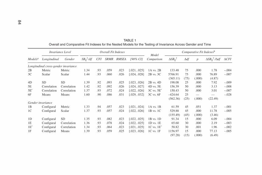
Overall fit indexes indicate good configural invariance of the AMS across wavesand gender (Model 1A). Although SBχ2 was statistically significant, the other in-dexes are satisfactory (SBχ2/df = 1.33; CFI = .94; SRMR = .056; RMSEA = .023).Table 1 presents overall and comparative fit indexes for measurement models de-picted in Figure 1 (a and b).

A general 2 × 3 MI. Overall fit indexes (SBχ2/df = 1.34; CFI = .93; SRMR =.059; RMSEA = .023), as well as CFIs (∆SBχ2/∆df = 1.78; /∆CFI = –.004), pro-vided good support for metric invariance across both waves and gender (Model2B). Concerning scalar invariance (Model 3C), overall fit indexes were similar tothose for the baseline and the metric invariance model (SBχ2/df = 1.44; CFI = .93;SRMR = .060; RMSEA = .026) and ∆CFI was lower than –.01. However, ∆SBχ2

values were particularly “large.” This is likely due to the asymptomatic nature thatmakes ∆SBχ2 statistics oversensitive (see Discussion section). The ∆χ2 statisticswere less sensitive. On the other hand, a ∆CFI = –.007 provides support for a satis-factory scalar invariance.

Looking at gender and longitudinal invariance separately, results indicate thatmetric invariance was stronger across gender (Model 1B) than waves (Model 2A).Indeed, there was no significant difference in SBχ2 and CFIs with the addition ofinvariance constraints to loadings across gender (∆SBχ2 = 61.59; p = .051; ∆SBχ2/∆df = 1.37; ∆CFI = –.001). Concerning longitudinal invariance, although ∆SBχ2

was significant, other fit indexes remained good (e.g., ∆SBχ2/∆df = 1.93; ∆CFI =–.004). A similar pattern was observed at the scalar level, such that comparativestatistics were better for gender (Model 1C; ∆χ2/∆df = 3.46; ∆SBχ2/∆df = 11.78;∆CFI = –.005) than longitudinal (Model 3A; ∆χ2/∆df = 5.18; ∆SBχ2/∆df = 111.09;∆CFI = –.004) invariance tests (see Table 1).


84

TABLE 1Overall and Comparative Fit Indexes for the Nested Models for the Testing of Invariance Across Gender and Time

Invariance Level Overall Fit IndexesModel

Comparison

Comparative Fit Indexesb

Modelsa Longitudinal Gender SBχ2 /df CFI SRMR RMSEA [90% CI] ∆SBχ2 ∆df p ∆SBχ2 /∆df ∆CFI

Longitudinal cross-gender invariance2B Metric Metric 1.34 .93 .059 .023 [.021, .025] 1A vs. 2B 133.48 75 .000 1.78 –.0043C Scalar Scalar 1.44 .93 .060 .026 [.024, .028] 2B vs. 3C 5766.91

(365.11)75

(75).000

(.000)76.89(4.87)

–.007

4D SD SD 1.39 .92 .093 .025 [.023, .026] 2B vs. 4D 198.08 25 .000 7.92 –.0095E Correlation Correlation 1.42 .92 .092 .026 [.024, .027] 4D vs. 5E 156.39 50 .000 3.13 –.0085E′ Correlation Correlation 1.37 .93 .072 .024 [.022, .026] 3C vs. 5E′ 150.43 50 .000 3.01 –.0076F Means Means 1.60 .90 .086 .031 [.029, .032] 3C vs. 6F –424.64

(562.36)25

(25)—

(.000)—

(22.49)–.028

Gender invariance1B Configural Metric 1.33 .94 .057 .023 [.021, .024] 1A vs. 1B 61.59 45 .051 1.37 –.0011C Configural Scalar 1.37 .93 .057 .024 [.022, .026] 1B vs. 1C 529.88

(155.49)45

(45).000

(.000)11.78(3.46)

–.005

1D Configural SD 1.35 .93 .082 .023 [.022, .025] 1B vs. 1D 91.34 15 .000 6.09 –.0041E Configural Correlation 1.36 .93 .078 .024 [.022, .025] 1D vs. 1E 65.60 30 .000 2.19 –.0031E′ Configural Correlation 1.34 .93 .064 .023 [.021, .025] 1C vs. 1E′ 58.82 30 .001 1.96 –.0021F Configural Means 1.39 .93 .059 .025 [.023, .026] 1C vs. 1F 1156.97

(97.28)15

(15).000

(.000)77.13(6.49)

–.005

85

Gender invariance in 8th grade1B–8th Configural Metric in 8th 1.33 .94 .056 .023 [.021, .024] 1A vs. 1B 12.12 15 .670 .81 .0001C–8th Configural Scalar in 8th 1.33 .94 .056 .023 [.021, .024] 1B vs. 1C 36.72

(25.45)15

(15).001

(.044)2.24

(1.70).000

1D–8th Configural SD in 8th 1.34 .94 .062 .023 [.021, .025] 1B vs. 1D 38.96 5 .000 7.79 –.0021E–8th Configural Corr. in 8th 1.34 .93 .062 .023 [.021, .025] 1D vs. 1E 32.90 10 .000 3.29 –.0021E′–8th Configural Corr. in 8th 1.33 .94 .060 .023 [.021, .025] 1C vs. 1E′ 26.33 10 .003 2.63 –.0011F–8th Configural Means in 8th 1.35 .94 .057 .023 [.021, .025] 1C vs. 1F –87.11

(58.53)5

(5)—

(.000)—

(11.71)–.003

Gender invariance in 9th grade1B–9th Configural Metric in 9th 1.33 .94 .056 .023 [.021, .024] 1A vs. 1B 14.76 15 .469 .98 .0001C–9th Configural Scalar in 9th 1.34 .93 .056 .023 [.021, .025] 1B vs. 1C 2497.13

(64.92)15

(15).000

(.000)166.48

(4.33)–.003

1D–9th Configural SD in 9th 1.33 .94 .061 .023 [.021, .025] 1B vs. 1D 13.94 5 .016 2.79 –.0011E–9th Configural Corr. in 9th 1.33 .94 .061 .023 [.021, .025] 1D vs. 1E 19.46 10 .035 1.95 –.0011E′–9th Configural Corr. in 9th 1.33 .94 .058 .023 [.021, .024] 1C vs. 1E′ 19.70 10 .032 1.97 –.0011F–9th Configural Means in 9th 1.35 .94 .056 .023 [.021, .025] 1C vs. 1F 44.19

(19.40)5

(5).000

(.002)8.84

(3.88)–.001

Gender invariance in 10th grade1B–10th Configural Metric in

10th1.33 .94 .057 .023 [.021, .025] 1A vs. 1B 31.58 15 .007 2.11 –.001

1C–10th Configural Scalar in10th

1.35 .93 .057 .023 [.022, .025] 1B vs. 1C 488.30(65.58)

15(15)

.000(.000)

32.55(4.37)

–.002

1D–10th Configural SD in 10th 1.35 .93 .073 .023 [.021, .025] 1B vs. 1D 89.58 5 .000 17.92 –.0031E–10th Configural Corr. in 10th 1.35 .93 .070 .023 [.021, .025] 1D vs. 1E 24.53 10 .006 2.45 –.0011E′–10th Configural Corr. in 10th 1.34 .94 .059 .023 [.021, .025] 1C vs. 1E′ 22.71 10 .012 2.27 –.0011F–10th Configural Means in

10th1.37 .93 .058 .024 [.022, .026] 1C vs. 1F –74.84

(64.97)5

(5)—

(.001)—

(12.99)–.004

(continued)

86

Longitudinal invariance2A Metric Configural 1.34 .93 .059 .023 [.021, .025] 1A vs. 2A 115.96 60 .000 1.93 –.0043A Scalar Configural 1.42 .93 .060 .026 [.024, .027] 2A vs. 3A 6665.38

(310.69)60

(60).000

(.000)111.09

(5.18)–.006

4A SD Configural 1.37 .93 .075 .024 [.022, .026] 2A vs. 4A 134.91 20 .000 6.75 –.0065A Correlation Configural 1.39 .92 .079 .025 [.023, .026] 4A vs. 5A 108.84 40 .000 2.72 –.0055A′ Correlation Configural 1.36 .93 .067 .024 [.022, .026] 3A vs. 5A′ 113.98 40 .000 2.85 –.0056A Means Configural 1.58 .90 .079 .030 [.028, .032] 3A vs. 6A –305.01

(526.46)20

(20)—

(.000)—

(26.32)–.027

Longitudinal invariance for girls (G)2A-G Metric for

girlsConfigural 1.34 .93 .058 .023 [.021, .025] 1A vs. 2A 68.82 30 .000 2.29 –.003

3A-G Scalar forgirls

Configural 1.39 .93 .059 .025 [.023, .026] 2A vs. 3A 24185.03(167.61)

30(30)

.000(.000)

806.17(5.59)

–.005

4A-G SD for girls Configural 1.36 .93 .067 .024 [.022, .025] 2A vs. 4A 62.71 10 .000 6.27 –.0045A-G Corr. for

girlsConfigural 1.37 .93 .067 .024 [.022, .026] 4A vs. 5A 47.93 20 .000 2.40 –.002

5A′-G Corr. forgirls

Configural 1.35 .93 .060 .023 [.022, .025] 3A vs. 5A′ 52.38 20 .000 2.62 –.002

6A-G Means forgirls

Configural 1.47 .92 .067 .027 [.025, .029] 3A vs. 6A –150.33(270.80)

10(10)

—(.000)

—(27.08)

–0.14

TABLE 1 (Continued)

Invariance Level Overall Fit IndexesModel

Comparison

Comparative Fit Indexesb

Modelsa Longitudinal Gender SBχ2 /df CFI SRMR RMSEA [90% CI] ∆SBχ2 ∆df p ∆SBχ2 /∆df ∆CFI

87

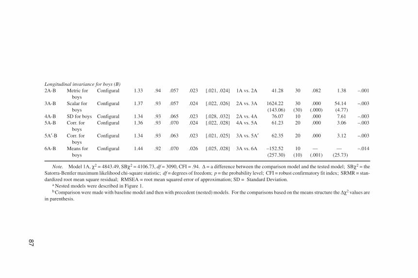
Longitudinal invariance for boys (B)2A-B Metric for

boysConfigural 1.33 .94 .057 .023 [.021, .024] 1A vs. 2A 41.28 30 .082 1.38 –.001

3A-B Scalar forboys

Configural 1.37 .93 .057 .024 [.022, .026] 2A vs. 3A 1624.22(143.06)

30(30)

.000(.000)

54.14(4.77)

–.003

4A-B SD for boys Configural 1.34 .93 .065 .023 [.028, .032] 2A vs. 4A 76.07 10 .000 7.61 –.0035A-B Corr. for

boysConfigural 1.36 .93 .070 .024 [.022, .028] 4A vs. 5A 61.23 20 .000 3.06 –.003

5A′-B Corr. forboys

Configural 1.34 .93 .063 .023 [.021, .025] 3A vs. 5A′ 62.35 20 .000 3.12 –.003

6A-B Means forboys

Configural 1.44 .92 .070 .026 [.025, .028] 3A vs. 6A –152.52(257.30)

10(10)

—(.001)

—(25.73)

–.014

Note. Model 1A, χ2 = 4843.49, SBχ2 = 4106.73, df = 3090, CFI = .94. ∆ = a difference between the comparison model and the tested model; SBχ2 = theSatorra-Bentler maximum likelihood chi-square statistic; df = degrees of freedom; p = the probability level; CFI = robust confirmatory fit index; SRMR = stan-dardized root mean square residual; RMSEA = root mean squared error of approximation; SD = Standard Deviation.

a Nested models were described in Figure 1.b Comparison were made with baseline model and then with precedent (nested) models. For the comparisons based on the means structure the ∆χ2 values are

in parenthesis.

Cross-gender MI across waves. Although previous results clearly indi-cated a good level of metric and scalar invariance across gender, it could be inter-esting to examine whether such invariance was constant across grade levels. First,concerning metric invariance, the difference in SBχ2 was smaller (indicating ahigher degree of invariance) in 8th grade (∆SBχ2 = 12.12, p = .670), than in 9thgrade (∆SBχ2 = 14.76, p = .467), and than in 10th grade (∆SBχ2 = 31.58, p = .007).As students aged, more subtle “variances” appeared between boys and girls. Sec-ond, concerning scalar invariance, the examination of chi-square differences(rather than SBχ2 differences) indicated a somewhat similar pattern in which moresubtle variance appeared in 9th grade (∆χ2 = 64.92, p < .001; ∆SBχ2 = 2497.13, p <.001) and 10th grade (∆χ2 = 65.58, p < .001; ∆SBχ2 = 488.30, p < .001) than in 8thgrade (∆χ2 = 25.45, p < .044; ∆SBχ2 = 36.72, p < .001). These variations acrosswaves can also be observed in ∆CFIs.6

Longitudinal MI across gender. Because longitudinal invariance was lessstrongly reached, it is particularly interesting to examine whether gender couldmoderate this result. Results in Table 1 clearly indicate that metric invariance hy-pothesis was more supported in the boy sample (∆SBχ2 = 41.28; p = .08; ∆CFI =–.001) than in the girl sample (∆SBχ2 = 68.82, p < .001; ∆CFI = –.003). This differ-ence between boys and girls was also obtained in scalar invariance tests (∆χ2 =167.60 vs. 143.06, ps < .001; ∆SBχ2 = 1624.22 vs. 24185.03, ps < .001; ∆CFI =–.003 vs. –.005).

Interactional MI. We examined the impact of invariance constraints acrossgender on longitudinal invariance tests, and vice versa. For instance, the probabil-ity of rejecting cross-gender metric invariance was lower when constraints for lon-gitudinal metric invariance were previously added (Model 2A vs. Model 2B;∆SBχ2 = 17.75; p = .276; ∆SBχ2/∆df = 1.18) than when they were not (Model 1Avs. Model 1B; ∆SBχ2 = 61.59; p = .051; ∆SBχ2/∆df = 1.78). Similarly, when ex-amining cross-gender scalar invariance, ∆CFI was lower when constraints relatedto longitudinal scalar invariance were previously added (Model 3B vs. Model 3C;∆CFI = .000) than when they were not (Model 1B vs. Model 1C; ∆CFI = –.005).The inverse pattern seemed to appear for longitudinal invariance whencross-gender invariance constraints were added. For instance, when examiningmetric invariance, ∆SBχ2/∆df ratio was higher when constraints related tocross-gender metric invariance were previously added (Model 1B vs. Model 2B;∆SBχ2/∆df = 2.53) than when they were not (Model 1A vs. Model 2A; ∆SBχ2/∆df= 1.93).


6It should be noted that these comparisons of the fit differences (as well as the next ones) are not sta-tistical and, thus, somewhat arbitrated (see Discussion section).

This last result can be explained by the stronger metric invariance across genderthan waves. Indeed, because the tests for cross-gender and longitudinal invarianceshared common constraints (30 exactly; see Method section), CFIs can be differentdepending on which model they are based, than on models that do not account forthese confounding constraints or on models in which these common constraintswere previously added. Therefore, researchers need to pay attention to whichnested models they used to test FI. The presence of shared common parameterscould influence the meaning of the FI tests.

Latent Standard Deviation Invariance (LSDI)

A general 2 × 3 LSDI. Overall and comparative fit indexes indicate the ex-istence of a few degrees of variance in latent motivational factors’ standard devia-tions (Model 4D). Indeed, although RMSEAs were below cutoff criteria, SRMRwas higher than .09 and ∆CFI was very close to –.01 cutoff criteria. When distin-guishing longitudinal and cross-gender invariance, fit indexes were more satisfac-tory but still revealed some variance. For instance, ∆SBχ2/∆df ratios were higherthan 6.00 (Models 1D and 4A).

Cross-gender LSDI across waves. As observed with scalar invariance, itseemed that cross-gender invariance was stronger in 9th grade than in 8th and 10thgrade, ∆SBχ2/∆df ratio in 10th grade being particularly high (i.e., 17.92). The ex-amination of standard deviation parameters for each motivational construct (Table2) revealed that the lower degree of invariance in 8th grade was due to a lower stan-dard deviation for external regulation for boys than girls (∆σ = –.27), and a higheramotivation’s standard deviation for boys than girls (∆σ = +.35). In 10th grade, dif-ferences were mainly found for the amotivation’s standard deviation, which wassignificantly lower for girls (i.e., σ = .76) than boys (i.e., σ = 1.24), ∆χ2 = 20.04, p< .001. Although this stronger homogeneity in girls’ reported amotivation thanboys’ was also observed in 8th and 9th grade, differences between standard devia-tions were less important (in 8th grade ∆σ = 1.35–1.00 = .35; in 9th grade ∆σ =1.49–1.20 = .29; in 10th grade ∆σ = 1.24–0.76 = .48).

Longitudinal LSDI across gender. Longitudinal invariance of standard de-viation was somewhat stronger for girls than boys (e.g., ∆SBχ2/∆df = 6.27 vs.7.61), but this difference did not appear in ∆CFI. Examining relative standard devi-ations (Table 2) revealed that the longitudinal variations were present mainly inidentified regulation and amotivation. For instance, among girls, standard devia-tions for identified regulation and amotivation seemed to increase from 8th to 9thgrade and then decrease from 9th to 10th grade. A similar pattern can be observedfor boys’ amotivation, but boys remained heterogeneous in their identified regula-tion.


Latent Correlation Invariance (LCI)

Because of the existence of a slightly variation at the standard deviation level, itcould be preferable to examine LCI when latent standard deviation parameterswere not constrained across gender and time (Model 5E′). Therefore, the fit in-dexes for models with and without standard deviation constraints (i.e., Model 5Eand Model 5E′, respectively) are reported in Table 1.

A general 2 × 3 LCI. Overall fit indexes were satisfactory (Model 5E′: CFI= .93; RMSEA = .024; SRMR = .072). On the other hand, CFIs indicate the exis-tence of a few degrees of variance in intercorrelations. Although ∆CFI was –.008(i.e., below the –.01 cutoff but higher than the other ∆CFIs), ∆SBχ2/∆df ratio washigher than 3.00. However, when distinguishing longitudinal and cross-genderinvariance, fit indexes were more satisfactory, ∆SBχ2/∆df ratios being lower than3.00.

Cross-gender LCI across waves. The examination of cross-gender invari-ance in correlations revealed gender differences in correlations among motiva-tional constructs mainly in 8th grade (∆SBχ2/∆df = 2.63). For instance, correla-tions between amotivation and the other constructs were higher for girls (from –.06


TABLE 2Latent Standard Deviation for Each Motivational Construct

Latent Standard Deviation

8th Grade 9th Grade 10th Grade

Intrinsic motivationGirls 1.00a 1.09 1.05Boys 1.00 1.07 1.03

Identified regulationGirls 1.00a 1.30 1.14Boys 0.98 1.44 1.38

Introjected regulationGirls 1.00a 1.15 1.08Boys 1.15 1.15 1.16

External regulationGirls 1.00a 0.91 0.97Boys 0.73 1.01 0.94

AmotivationGirls 1.00a 1.20 0.76Boys 1.35 1.49 1.24

Note. Loadings are constrained to be equal across gender and waves.a Fixed parameters.

to –.54) than for boys (from .00 to –.24) (see Table 3). When correlation invariancewas tested in 8th grade including constraints on correlations other than those in-volving amotivation, ∆SBχ2 was not statistically significant, ∆SBχ2(∆df = 6) =16.37, p = .012. These differences were also present in 9th and 10th grade but werenot as large.

Longitudinal LCI across gender. As observed for standard deviations,girls’ correlations were more longitudinally invariant than boys’ (∆SBχ2/∆df =2.62 vs. 3.12). Examining correlation patterns (Table 3), it was observed that thelarger differences in the boy sample were due to correlations between amotivationand the other constructs, especially between 9th and 10th grade. When“9th-to-10th-grade” constraints on correlations between amotivation and the otherconstructs were relaxed, ∆SBχ2 was statistically nonsignificant, ∆SBχ2(∆df = 16)= 38.20, p = .001.

Latent Mean Invariance

In this section, the results from latent mean invariance tests (Table 1) are describedfirst. Due to noninterpretable ∆SBχ2 statistics (see Discussion section), overall fitindexes as well as ∆CFIs and ∆χ2 statistics are focused on. Although it was not thepurpose of this article, interpreted observed differences are then interpreted. Table4 reports latent correlations when loadings and intercepts were constrained to beequal across gender and waves.

Invariance tests. Results from longitudinal cross-gender invariance tests in-dicated differences in latent means (∆CFI = –.028; ∆SBχ2(∆df = 25) = 562.36, p <.001). Distinguishing longitudinal and gender effects, it was observed that latentmean differences were particularly significant across waves (∆CFI = –.027;∆SBχ2(∆df = 20) = 526.46, p < .001) and less significant across gender (∆CFI =–.005; ∆SBχ2(∆df = 15) = 97.28, p < .001). More specific invariance tests revealedthat latent mean differences between girls and boys were higher in 8th and 10thgrades (∆CFIs = –.003 and –.004; ∆SBχ2(∆df = 5) = 58.53 and 64.97, ps < .001)than in 9th grade (∆CFI = –.001; ∆SBχ2(∆df = 5) = 19.40, p = .002). However, itshould be noted that although intercept invariance was less evident in 9th gradethan in others waves (see previous), intercepts were constrained to be equal acrosssamples. Therefore, any gender differences in raw scores that could be observed in9th grade should be therefore mainly interpreted in terms of an intercept differencerather than a construct difference. This was less true in 8th and 10th grade. Longi-tudinal invariance was equivalent in both girl and boy samples (∆CFIs = –.014).

Latent means interpretation. Table 4 revealed the existence of various 2 ×3 latent mean patterns depending on the motivational constructs. For instance,


92

TABLE 3Latent Correlations Among Motivational Constructs for Girls (Upper Diagonal) and for Boys (Lower Diagonal)


(1) (2) (3) (4) (5) (1) (2) (3) (4) (5) (1) (2) (3) (4) (5)

Intrinsic motivation (1) — .80(.78)

.63(.56)

.30(.20)

–.59(–.54)

— .72(.73)

.72(.72)

.46(.49)

–.47(–.47)

— .81(.78)

.65(.64)

.17(.16)

–.67(.64)

Identified regulation (2) .70(.70)

— .68(.64)

.73(.72)

–.55(–.49)

.71(.74)

— .59(.60)

.90(.92)

–.45(–.45)

.71(.73)

— .65(.65)

.57(.60)

–.67(–.61)

Introjected regulation (3) .78(.77)

.59(.58)

— .57(.54)

–.38(–.27)

.78(.78)

.57(.58)

— .54(.60)

–.35(–.34)

.62(.61)

.51(.50)

— .49(.49)

–.35(.33)

External regulation (4) .39(.31)

.83(.79)

.42(.36)

— –.15(–.06)

.47(.53)

.89(.89)

.45(.49)

— –.18(–.21)

.23(.29)

.71(.73)

.29(.33)

— –.03(–.04)

Amotivation (5) –.21(–.24)

–.20(–.26)

–.09(–.10)

–.01(.00)

— –.26(–.32)

–.47(–.53)

–.07(–.10)

–.26(–.31)

— –.47(–.51)

–.69(–.72)

–.23(–.22)

–.25(–.30)

—

Note. Loadings and latent standard deviations are constrained to be equal across gender and waves. In parenthesis only loadings are constrained to be equalacross gender and waves.

latent means for intrinsic motivation, identified regulation, and introjected regula-tion decreased from 8th to 10th grade and were higher for girls than boys. How-ever, interactions can be observed only in ID latent means where gender differ-ences were absent in 8th grade but significant in 9th grade and largest in 10thgrade. Concerning external regulation, boys’ latent means consistently decreasedfrom 8th to 10th grade, whereas girls’ external regulation increased from 8th to 9thgrade and then decreased from 9th to 10th grade. The combination of these twopatterns resulted in gender differences (boys’ being higher than girls’) only in 8thand 10th grade. Finally, both girls’ and boys’ amotivation latent means increasedduring the first period (8th to 9th grade) and then decreased in the second period(9th to 10th grade).

DISCUSSION AND CONCLUSION

The purpose of this study was to evaluate the longitudinal cross-gender FI of theAMS (Vallerand et al., 1989, 1992, 1993). A second related purpose was to presentan integrated analytical strategy to test both longitudinal (across 3 years) andcross-gender FI of a multidimensional scale in one set of nested models. This 2 × 3design allowed us to test specific hypotheses concerning cross-sample FI for each


TABLE 4Latent Means For Each Motivational Construct

Latent Means


Intrinsic motivationGirls .00a –.52 –.88Boys –.24 –.63 –1.10

Identified regulationGirls .00a –.39 –.66Boys .04 –.69 –1.09

Introjected regulationGirls .00a –.33 –.78Boys –.28 –.53 –1.17

External regulationGirls .00a .17 –.23Boys .44 .15 –.01

AmotivationGirls .00a .45 .02Boys .29 .81 .49

Note. Loadings and intercepts are constrained to be equal across gender and waves.aFixed parameters.

wave, as well as the comparison of longitudinal FI in the boy and girl samples.These results have also implications for FI research.

Implications for AMS Validation

These results provide support for longitudinal cross-gender metric invariance, aswell as satisfactory support for scalar invariance of the AMS. Therefore, we rec-ommend using this scale to test specific hypotheses about gender differences aswell as motivational development. More specific results revealed that cross-genderinvariance was slightly stronger than longitudinal invariance. Furthermore, subtlecross-gender variance appeared in the measure as students became older. Becauselongitudinal invariance seemed to be stronger for boys than for girls, one can con-clude that girls subjectively redefined the motivational construct, whereas boysseemed to be constant. We propose two types of explanations for this finding.

First, the difference found in the redefinition of motivational constructs may bedue to developmental differences between girls and boys. Indeed, the period from8th to 10th grades coincides with early adolescence and girls usually reach puber-tal maturity earlier than boys. Because of the complexity of the constructs, mea-surement characteristics may change during childhood, perhaps differently forgirls and boys. An alternative explanation concerns familiarity with the motiva-tional questionnaire. Girls might readjust their responses, whereas boys tended toremain constant in their definition of the constructs. Fortunately, FI tests were stillsatisfactory and allow further tests at the latent construct level.

Other interesting results are related to the latent constructs. For instance,whereas girls were more heterogeneous in amotivation than boys, the reverse wasobserved for external regulation. Furthermore, the 9th grade appears to be develop-mentally significant for girls because they were more heterogeneous in identifiedregulation and amotivation only during this wave compared to boys. This last find-ing can be explained by the previous results obtained with metric invariance. Al-though we obtained a satisfactory degree of metric invariance, the similarity in pat-tern that we observed in metric and standard deviations invariance tests couldreveal the influence of the former on the later. However, once again an alternativeexplanation concerns maturity. Perhaps girls developed a relatively higher degreeof maturity in 9th grade than boys. Further examination of data in 11th and 12thgrade will be needed to test this hypothesis and to verify if a higher degree in boys’standard deviation will be observed later than girls.

Implications for Testing FI Within Structural EquationModeling Framework

The second purpose of this study was to demonstrate how to test both longitudinaland cross-gender factorial invariance of a multidimensional scale in one set of


nested models. Notably, five points should be emphasized. First, this analyticalstrategy distinguished measurement and latent construct components of the facto-rial model (see e.g., T.D. Little, 1997).

Second, a specific approach to solve identification problems in covariance andmean structures was used. Specifically, this study proposed, first, to fix factor vari-ance and means in one referent group, and then, to constrain the loading and inter-cept of one item to be equal across samples and waves. In addition to the fact thatthis approach could be equivalent to others in testing global (rather than partial)MI, the proposed approach is particularly pertinent for testing latent constructinvariance in a 2 × 3 design.

Third, this study also represented an opportunity to examine the efficacy of var-ious comparative indexes for comparing two nested models. Concerning the differ-ence between two SBχ2 statistics, although the test seemed appropriate for testingrestrictions in covariance structure, ∆SBχ2 values were noninterpretable when re-strictions were on mean structure (i.e., intercepts and latent means). Satorra andBentler (2001) suggested that ∆SBχ2 values (especially difference in scaling cor-rections) may turn out to be large or negative in particularly extreme cases, such aswhen sample size is small or when a less restricted model is “too deviant from thetrue model” (p. 511). Although these two extreme cases could pertain to this study,results clearly indicated that the analysis of a mean structure (in addition to acovariance structure) could also provide a source of explanation. Further researchis needed to examine the behavior of ∆SBχ2 and the conditions when it can be ap-plied to test invariance in a mean structure.

Fourth, this study also used the ∆SBχ2/∆df ratio as a CFI. Like the well-knownχ2/df ratio, the ratio between the chi-square difference and the difference of de-grees of freedom is particularly useful to examine how two nested models differ.Moreover, the ratio allowed for a comparison among invariance tests, especiallywhen ∆dfs varied. Because the ∆SBχ2/∆df ratio is relatively new in invariance test-ing, further examination in simulation studies is needed. Concerning the ∆CFIs, al-though only Cheung and Rensvold (1999) have appropriately studied the change inCFI as an indicator of (in)variance and further studies are needed, this test discrim-inated well among the various degrees of variance that were found in the study. Inparticular, the ∆CFI was more appropriate for invariance testing in mean structurethan the SBχ2 statistics. Finally, it is important to stress the importance of the useof various overall and comparative fit indexes to deduce the invariance of any pa-rameters across samples, waves, or both.

Finally, in examining cross-gender invariance across waves and longitudinalinvariance across gender, the relative fit loss (i.e., ∆SBχ2, ∆SBχ2/∆df ratio, and∆CFI) was compared. For example, the study showed that the gender difference inSBχ2 (for cross-gender metric invariance) was smaller in 8th grade than in 9thgrade and than in 10th grade (see section Cross-Gender MI across waves). How-ever, it is important to note that these comparisons are not statistical comparisons


and, thus, are somewhat arbitrated. Further research is needed to find a statisticalmethod for comparing two invariance tests (e.g., two ∆χ2) and to determine whatconstitutes a significant difference.

To conclude, we believe that this article and its associated results provide strongsupport for the use of the AMS to compare the motivation of girls and boys, as wellas to compare across grade levels. Finally, we hope that the reader will be con-vinced of the usefulness of the integrated analytical strategy that we propose.

ACKNOWLEDGMENTS

The data for this report comes from the Academic Motivation and Dropout Project(Pelletier, 2004). We thank the Conseil des Écoles Catholiques de LangueFrançaise de l’Est de l’Ontario for their collaboration on this project.

REFERENCES

Bentler, P. M. (1990). Comparative fit indexes in structural models. Psychological Bulletin, 107,238–246.

Bentler, P. M. (1995). EQS structural equations program manual. Encino, CA: Multivariate Software.Bollen, K. A. (1989). Structural equations with latent variables. New York: Wiley.Browne, M. W., & Cudeck, R. (1992). Alternative ways of assessing model fit. Sociological Methods

and Research, 21, 230–258.Cheung, G. W., & Rensvold, R. B. (1999). Testing factorial invariance across groups: A

reconceptualization and proposed new method. Journal of Management, 25, 1–27.Cheung, G. W., & Rensvold, R. B. (2002). Evaluating goodness-of-fit indexes for testing measurement

invariance. Structural Equation Modeling, 9, 233–255.Deci, E. L. (1975). Intrinsic motivation. New York: Plenum.Deci, E. L., & Ryan, R. M. (1985). Intrinsic motivation and self-determination in human behavior. New

York: Plenum.Deci, E. L., & Ryan, R. M. (2000). The “what” and “why” of goal pursuits: Human needs and the

self-determination of behavior. Psychological Inquiry, 11, 227–268.Deci, E. L., Vallerand, R. J., Pelletier, L. G., & Ryan, R. M. (1991). Motivation and education: The

self-determination perspective. Educational Psychologist, 26, 325–346.Guay, F., & Vallerand, R. J. (1997). Social context, student’s motivation, and academic achievement:

Toward a process model. Social Psychology of Education, 1, 211–233.Harter, S. (1981). A new self-orientation scale of intrinsic versus extrinsic orientation in the classroom:

Motivational and informational components. Developmental Psychology, 17, 300–312.Hu, L., & Bentler, P. M. (1999). Cutoff criteria for fit indexes in covariance structure analysis: Conven-

tional criteria versus new alternatives. Structural Equation Modeling, 6, 1–55.Jamshidian, M., & Bentler, P. M. (1999). ML estimation of mean and covariance structures with miss-

ing data using complete data routines. Journal of Educational and Behavioral Statistics, 24, 21–41.Kim, K. H., & Bentler, P. M. (2002). Tests of homogeneity of means and covariance matrices for

multivariate incomplete data. Psychometrika, 67, 609–624.Little, R. J. A., & Rubin, D. B. (1987). Statistical analysis with missing data. New York: Wiley.


Little, T. D. (1997). Mean and covariance structures (MACS) analyses of cross-cultural data: Practicaland theoretical issues. Multivariate Behavioral Research, 32, 53–76.

Marsh, H. W., Hau, K.-T., & Wen, Z. (2004). In search of golden rules: Comment on hypothesis-testingapproaches to setting cutoff values for fit indexes and dangers in overgeneralizing Hu and Bentler’s(1999) findings. Structural Equation Modeling, 11, 320–341.

McArdle, J. J., & Cattell, R. B. (1994). Structural equation models of factorial invariance in parallelproportional profiles and oblique confactor problems. Multivariate Behavioral Research, 29,63–113.

Meredith, W. (1993). Measurement invariance, factor analysis and factorial invariance. Psychometrika,58, 525–543.

Muthén, B., Kaplan, D., & Hollis, M. (1987). On structural equation modeling with data that are notmissing completely at random. Psychometrika, 52, 431–462.

Nevitt, J., & Hancock, G. R. (2000). Improving the root mean square error of approximation fornonnormal conditions in structural equation modeling. The Journal of Experimental Education, 68,251–268.

Pelletier, L. G. (2004). Academic motivation and dropout in Ottawa elementary and high school(2000–2004). Report submitted to Le Conseil des Écoles Catholiques de Langue Française de l’Estde l’Ontario, University of Ottawa, Ontario, Canada.

Pelletier, L. G., Séguin-Lévesque, C., & Legault, L. (2002). Pressure from above and pressure from be-low as determinants of teachers’motivation and teaching behaviors. Journal of Educational Psychol-ogy, 94, 186–196.

Reise, S. P., Widaman, K. F., & Pugh, R. H. (1993). Confirmatory factor analysis and item response the-ory: Two approaches for exploring measurement invariance. Psychological Bulletin, 114, 552–566.

Satorra, A. (2000). Scaled and adjusted restricted tests in multisample analysis of moment structures. InD. D. H. Heijmans, D. S. G. Pollock, & A. Satorra (Eds.), Innovations in multivariate statisticalanalysis: A Festschrift for Heinz Neudecker (pp. 233–247). Dordrecht, The Netherlands: Kluwer.

Satorra, A., & Bentler, P. M. (1988). Scaling corrections for chi-square statistics in covariance structureanalysis. 1988 Proceedings of the American Statistical Association, 308–313.

Satorra, A., & Bentler, P. M. (1994). Corrections to test statistics and standard errors in covariancestructure analysis. In A. von Eye & C. C. Clogg (Eds.), Latent variables analysis: Applications fordevelopmental research (pp. 399–419). Thousand Oaks, CA: Sage.

Satorra, A., & Bentler, P. M. (2001). A scaled difference chi-square test statistic for moment structureanalysis. Psychometrika, 66, 507–514.

Steenkamp, J.-B. E. M., & Baumgartner, H. (1998). Assessing measurement invariance incross-national consumer research. Journal of Consumer Research, 25, 78–90.

Steiger, J. H., & Lind, J. C. (1980, June). Statistically based tests for the number of common factors. Pa-per presented at the annual meeting of the Psychometric Society, Iowa City, IA.

Thompson, B. (2003). Score reliability: Contemporary thinking on reliability issues. Thousand Oaks,CA: Sage.

Thurstone, L. L. (1947). Multiple-factor analysis: A development and expansion of the vectors of mind.Chicago: University of Chicago Press.

Vallerand, R. J., Blais, M. R., Brière, N. M., & Pelletier, L. G. (1989). Construction et validation del’échelle de motivation en éducation (ÉMÉ) [Construction and validation of the Échelle de Motiva-tion en Éducation—ÉMÉ]. Canadian Journal of Behavioural Science, 21, 323–349.

Vallerand, R. J., Fortier, M. S., & Guay, F. (1997). Self-determination and persistence in a real-life set-ting: Toward a motivational model of high school dropout. Journal of Personality and Social Psy-chology, 72, 1161–1176.

Vallerand, R. J., Pelletier, L. G., Blais, M. R., Brière, N. M., Senécal, C. B., & Vallières, É. F. (1992).The academic motivation scale: A measure of intrinsic, extrinsic, and amotivation in education. Edu-cational and Psychological Measurement, 52, 1003–1017.


Vallerand, R. J., Pelletier, L. G., Blais, M. R., Brière, N. M., Senécal, C. B., & Vallières, É. F. (1993). Onthe assessment of intrinsic, extrinsic, and amotivation in education: Evidence on the concurrent andconstruct validity of the academic motivational scale. Educational and Psychological Measurement,53, 159–172.

Vandenberg, R. J., & Lance, C. E. (2000). A review and synthesis of the measurement invariance litera-ture: Suggestions, practices, and recommendations for organizational research. Organizational Re-search Methods, 3, 4–70.

Widaman, K. F., & Thompson, J. S. (2003). On specifying the null model for incremental fit indices instructural equation modeling. Psychological Methods, 8, 16–37.


Longitudinal Cross-Gender Factorial Invariance of the ...selfdeterminationtheory.org/SDT/documents/2006_GrouzetOtis... · differences in motivation between females and ... thus estimated

Documents