Policy Research Institute, Ministry of Finance, Japan, Public Policy Review, Vol.9, No.3, September 2013 553 Long-term Verification of Low Volatility Stock Investment Toru Yamada Senior Quantitative Analyst, Investment Research & Development Department, Nomura Asset Management Co.,Ltd. Abstract We verify the long-term performance of low-volatility stocks in the stock markets around the world. A reliable observation becomes possible on the respective stock markets in the United States from the 1920s, in Japan from the 50s and in other developed countries from the 70s, as we use indices by industry, instead of individual stocks. From the results of our verification, it is observed that low-volatility stock portfolios such as minimum variance portfolios show higher risk-adjusted returns in the long run than the market-value-weighted indices in almost all markets. The spread of returns between the above-mentioned two are broken into two parts; the low-volatility effect, which means that low-volatility stocks produce higher risk-adjustment returns in the future than high-volatility stocks, and the non-market capitalization weighted effect, which means that the more closely the price fluctuations of certain stocks are corresponding to the market-value-weighted indices, the lower their future performances are. More specifically, it seems that low-volatility stock portfolios realize a relatively high performance by holding many low-volatility stocks without weighting them by market value. Key words: portfolio management, equity strategy, low-volatility effect, minimum variance portfolio, non-market capitalization weighted JEL classification: G11 I. Introduction Low volatility investments in equity markets have been becoming popular. One reason is that this strategy has realized a stable performance compared to market indices such as TOPIX in continuing turmoil such as the subprime mortgage crisis, the bankruptcy of Lehman Brothers, and the Greek debt crisis. In addition, much literature has recently uncovered the low-volatility effect, which means lower volatile stocks tend to have higher expected return or similar expected return to other stocks. Related to the effect, the low-beta effect has also been reported, which replaces volatility by market sensitivity (beta). The findings of the effects would date back to in the late 1960s. Studies such as Black et al. (1972) reported on the low-beta effect in the US stock market at the time. They found it in an investigation that was intended to test the theoretical prediction of the CAPM, which is that higher beta assets have higher expected returns. According to Fama and French (2004), this contradiction the early stage of the CAPM faced has successfully been absorbed in the

Welcome message from author
This document is posted to help you gain knowledge. Please leave a comment to let me know what you think about it! Share it to your friends and learn new things together.
Transcript
Policy Research Institute, Ministry of Finance, Japan, Public Policy Review, Vol.9, No.3, September 2013 553
Long-term Verification of Low Volatility Stock Investment
Toru YamadaSenior Quantitative Analyst, Investment Research & Development Department, Nomura Asset Management Co.,Ltd.
Abstract
We verify the long-term performance of low-volatility stocks in the stock markets around the world. A reliable observation becomes possible on the respective stock markets in the United States from the 1920s, in Japan from the 50s and in other developed countries from the 70s, as we use indices by industry, instead of individual stocks.
From the results of our verification, it is observed that low-volatility stock portfolios such as minimum variance portfolios show higher risk-adjusted returns in the long run than the market-value-weighted indices in almost all markets. The spread of returns between the above-mentioned two are broken into two parts; the low-volatility effect, which means that low-volatility stocks produce higher risk-adjustment returns in the future than high-volatility stocks, and the non-market capitalization weighted effect, which means that the more closely the price fluctuations of certain stocks are corresponding to the market-value-weighted indices, the lower their future performances are. More specifically, it seems that low-volatility stock portfolios realize a relatively high performance by holding many low-volatility stocks without weighting them by market value.
Key words: portfolio management, equity strategy, low-volatility effect, minimum variance portfolio, non-market capitalization weighted
JEL classification: G11
I. Introduction
Low volatility investments in equity markets have been becoming popular. One reason is that this strategy has realized a stable performance compared to market indices such as TOPIX in continuing turmoil such as the subprime mortgage crisis, the bankruptcy of Lehman Brothers, and the Greek debt crisis. In addition, much literature has recently uncovered the low-volatility effect, which means lower volatile stocks tend to have higher expected return or similar expected return to other stocks. Related to the effect, the low-beta effect has also been reported, which replaces volatility by market sensitivity (beta).
The findings of the effects would date back to in the late 1960s. Studies such as Black et al. (1972) reported on the low-beta effect in the US stock market at the time. They found it in an investigation that was intended to test the theoretical prediction of the CAPM, which is that higher beta assets have higher expected returns. According to Fama and French (2004), this contradiction the early stage of the CAPM faced has successfully been absorbed in the
554 T Yamada / Public Policy Review
Black version of the CAPM (Black (1972)). It means that the positive relation between market beta and expected return is held but the relation is weaker than Sharpe-Lintner’s CAPM predicts, that is, a weak form of the low-beta effect was allowed.
Subsequently the study of the low-beta effects had declined while the CAPM was establishing popularity. Meanwhile, Haugen and Baker (1991) raised a question to the CAPM with the result that low volatile equity portfolios indicate superior performance to cap-weighted portfolios. Later, Clarke et al. (2006) and Blitz and Vliet (2007) showed the effectiveness of low volatility investments and the results gather attention to this investment strategy. Then, in the comprehensive analysis of global equity markets, including in emerging countries (Yamada and Uesaki (2009)), and in the analysis for multiple asset classes beyond equity (Frazzini and Pedersen (2010)), broad low-volatility effects have been reported.
As for the causes of the effects, Mehrling (2005) explains Black (1972) as follows: because most investors do not freely use leverage, which means here that an investor borrows money and takes a long position on risk assets such as equity, investors who want high investment gains generate strong demands on high risk assets. The demands raise the market prices of high risk assets to be overvalued compared to their real intrinsic value, and thus the investment profits decrease in the future. Conversely, investors who are satisfied with modest profits do not yield excess demands because they can just reduce riskier asset holding.
Sharpe (1991) and Markowitz (2005) also show that the assumption of unlimited borrowing capability is a critical condition for the market portfolio to become the most efficient portfolio.
We attempt to conduct performance tests of low volatility stock investment, and our contributions beyond the existing literatures are mainly as follows:
First, portfolio constituents are market capitalization weighted sector indices in global equity markets, not individual stocks. Primary advantages are that using sectors enables extended analysis which we have never had before and that the results can easily be adapted to actual investments for investors even if they hold a huge amount of assets.
Second, we test both the low-beta and low-volatility effects which have rarely been distinguished from each other. As a result, we believe the value-add of low volatility investing can be captured from multilateral points of view.
The rest of the paper is organized as follows. First we describe target universes, analysis methodologies, data sources, and so on. We run empirical analysis on the low-volatility effect and confirm its robustness. Then, we discuss the results with additional analysis. Finally we conclude the paper.
II. Methodologies
II-1. Target universe
We attempt to observe the low-volatility effects by constructing portfolios with the cap-weighted sector indices.
Policy Research Institute, Ministry of Finance, Japan, Public Policy Review, Vol.9, No.3, September 2013 555
One reason why individual stocks are not used here is that reliable market historical data of sector indices are available for a long-run. We investigate the US from the 1920s, Japan from the 1950s, the UK from the 1960s, and most developed countries from the 1970s. It will be interesting to know the performance profile of the low-volatility effect not only after developed countries enter their low-growth period but also in their high-growth period.
In addition, apparently extreme volatility of an individual stock can be observed due to various reasons such as rare trades and takeover bids. Furthermore, it should be noted that the results will be affected by the definition of the universe, stock price movements of high credit risk companies, companies involved in mergers and bankruptcy, and outliers in observations. If the number of assets increases, larger estimation errors in the covariance matrix tend to be involved, which are used in the calculation of minimum variance portfolios described later.
On the other hand, in general anomaly analysis, using individual stocks can derive higher effects than using sector indices because of higher freedom in analysis. In this respect, the observed low-volatility effect in our analysis can be regarded as a conservative estimate.
Honda and Takahashi (2011) use sector indices for analysis of the low volatility investment in the Japanese stock market. We aim for a more comprehensive analysis in terms of length of periods and breadth of markets.
II-2. Beta and volatility relationship
The low-beta and low-volatility effects that have been reported so far have generally been perceived in different contexts. The former effect is as a contradiction of the CAPM and the latter effect is as an anomaly. These two risk measures are related each other,
M
iii (1)
where M is the volatility of the market portfolio, and i , i , and i are security i’s market beta, correlation with the market portfolio, and volatility, respectively.
To divide beta into volatility and correlation, we can also capture the CAPM’s prediction; a higher beta asset is expected to have higher risk premium, in the context of volatility and correlation. Under Markowitz’s framework of mean-variance analysis, each can be parsed as risk premium yielded from diagonal and off-diagonal components of the covariance matrix, respectively.
Because most investors do not prefer high volatility assets, volatility should be rewarded a premium. That is the so-called “high risk, high return” relationship. According to standard finance theory, an asset whose price goes up when the economic condition is good and goes down when the condition is bad should require a high risk premium. In other words, an asset which has higher sensitivity on the market portfolio, which represents the aggregated holding assets of all investors, should have a higher risk premium. Thus, in a rational market, in addition to the high-volatility effect, the high-beta effect or high-correlation effect, which is defined as an asset that has high beta or high correlation with the market portfolio tends to
556 T Yamada / Public Policy Review
imply high expected return, is assumed.From another point of view, on the CAPM, equation (1) and the positive relationship
between an individual stock’s expected return and the market beta deliver the following equation,
Mii SRSR (2)
where iSR and MSR are security i’s and the market portfolio’s expected Sharpe ratio, respectively.
If the Sharpe ratio of the market portfolio is the highest as the theory implies, equation (2) represents a simple relationship: as a portfolio’s correlation with the maximum Sharpe ratio portfolio gets higher, its Sharpe ratio becomes higher.
We observe the three separate effects.
II-3. Data
In our analysis, we mainly target three equity markets: the US, Japan, and developed country markets. In addition, other markets are tested in the robustness check.
The US sector indices are obtained from Kenneth R. French’s Data Library1. Among several sector definitions in the library, we mainly use the broadest 49-sector definition. The 49 sectors start with 40 at the beginning of July 1926 and grow in number gradually, and finally all the sector returns become available with Health Care in July 1969.
The Japanese sector indices are obtained from Japan Securities Research Institute’s CD-ROM, which are defined as 28 sectors of the Tokyo Stock Exchange 1st section. This definition is based on the old version of the Tokyo Stock Exchange industry classification. Their returns were available from January 1952 for 27 sectors without Air Transportation and all the sectors became available in March 1970.
The developed country market’s sector indices are from the Datastream Global Equity Index. They are based on ICB’s(Industry Classification Benchmark) 41 sectors. In the single country analysis that we conduct later, 20 sector are used for the countries that have many constituents, that is, the US, Canada, the UK, Germany, France, and Japan, and 10 sectors are used for the rest.
The market betas and correlations are calculated against the capitalization weighted market index in each market. For example, the UK sector’s market betas are calculated against the UK market index.
The returns used here are defined as excess returns between total return in local currency and cash return in the same currency. In the cases of developed and emerging country markets, the returns are denominated in the US dollar.
The three factor returns of Fama and French (1993) are obtained from the Data Library
1 http://mba.tuck.dartmouth.edu/pages/faculty/ken.french/data_library.html
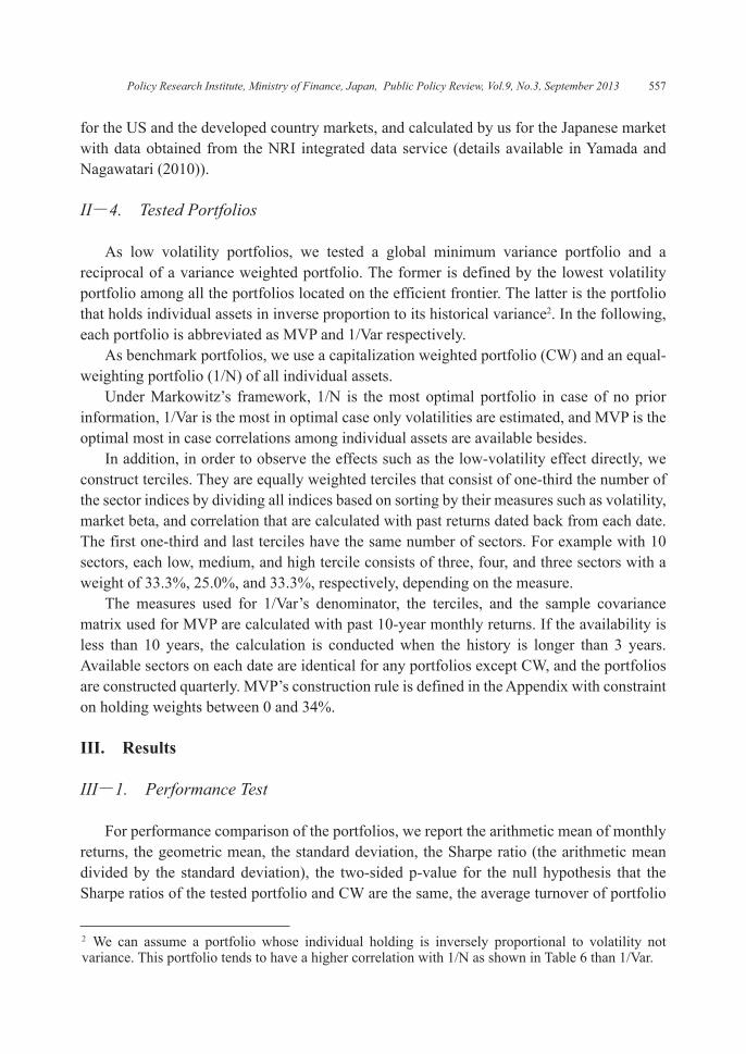
Policy Research Institute, Ministry of Finance, Japan, Public Policy Review, Vol.9, No.3, September 2013 557
for the US and the developed country markets, and calculated by us for the Japanese market with data obtained from the NRI integrated data service (details available in Yamada and Nagawatari (2010)).
II-4. Tested Portfolios
As low volatility portfolios, we tested a global minimum variance portfolio and a reciprocal of a variance weighted portfolio. The former is defined by the lowest volatility portfolio among all the portfolios located on the efficient frontier. The latter is the portfolio that holds individual assets in inverse proportion to its historical variance2. In the following, each portfolio is abbreviated as MVP and 1/Var respectively.
As benchmark portfolios, we use a capitalization weighted portfolio (CW) and an equal-weighting portfolio (1/N) of all individual assets.
Under Markowitz’s framework, 1/N is the most optimal portfolio in case of no prior information, 1/Var is the most in optimal case only volatilities are estimated, and MVP is the optimal most in case correlations among individual assets are available besides.
In addition, in order to observe the effects such as the low-volatility effect directly, we construct terciles. They are equally weighted terciles that consist of one-third the number of the sector indices by dividing all indices based on sorting by their measures such as volatility, market beta, and correlation that are calculated with past returns dated back from each date. The first one-third and last terciles have the same number of sectors. For example with 10 sectors, each low, medium, and high tercile consists of three, four, and three sectors with a weight of 33.3%, 25.0%, and 33.3%, respectively, depending on the measure.
The measures used for 1/Var’s denominator, the terciles, and the sample covariance matrix used for MVP are calculated with past 10-year monthly returns. If the availability is less than 10 years, the calculation is conducted when the history is longer than 3 years. Available sectors on each date are identical for any portfolios except CW, and the portfolios are constructed quarterly. MVP’s construction rule is defined in the Appendix with constraint on holding weights between 0 and 34%.
III. Results
III-1. Performance Test
For performance comparison of the portfolios, we report the arithmetic mean of monthly returns, the geometric mean, the standard deviation, the Sharpe ratio (the arithmetic mean divided by the standard deviation), the two-sided p-value for the null hypothesis that the Sharpe ratios of the tested portfolio and CW are the same, the average turnover of portfolio
2 We can assume a portfolio whose individual holding is inversely proportional to volatility not variance. This portfolio tends to have a higher correlation with 1/N as shown in Table 6 than 1/Var.
558 T Yamada / Public Policy Review
rebalancing, Jensen’s alpha, the two-sided p-value for the null hypothesis that the alpha is zero, and the market beta. The difference between arithmetic and geometric means is described in the Appendix.
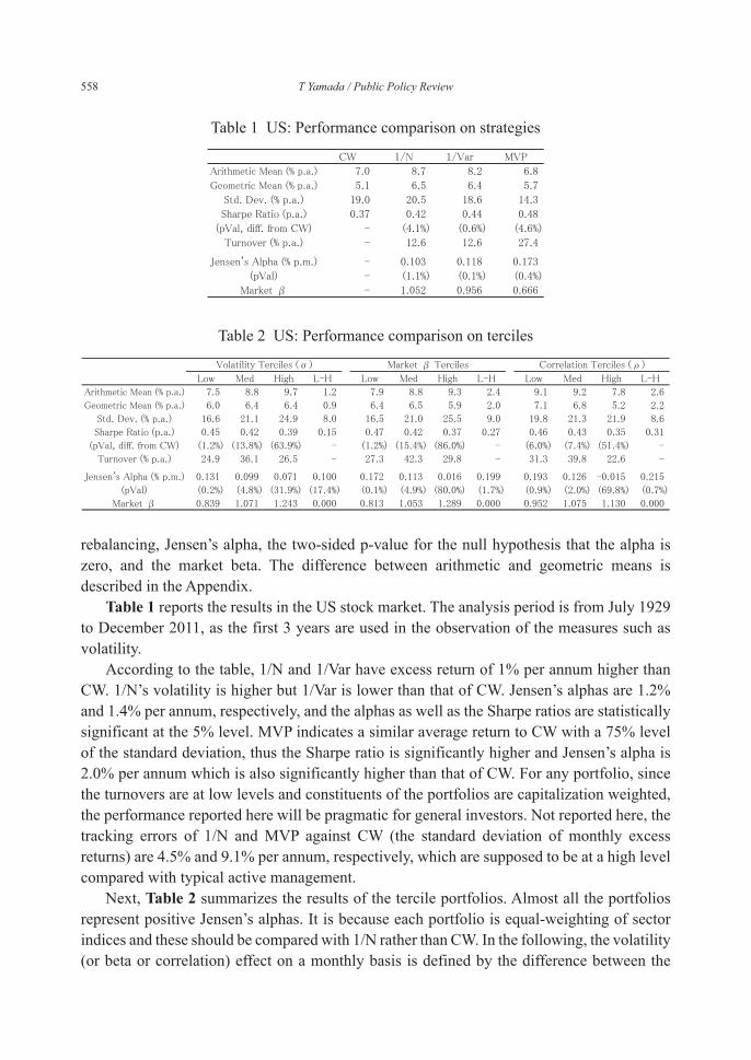
Table 1 reports the results in the US stock market. The analysis period is from July 1929 to December 2011, as the first 3 years are used in the observation of the measures such as volatility.
According to the table, 1/N and 1/Var have excess return of 1% per annum higher than CW. 1/N’s volatility is higher but 1/Var is lower than that of CW. Jensen’s alphas are 1.2% and 1.4% per annum, respectively, and the alphas as well as the Sharpe ratios are statistically significant at the 5% level. MVP indicates a similar average return to CW with a 75% level of the standard deviation, thus the Sharpe ratio is significantly higher and Jensen’s alpha is 2.0% per annum which is also significantly higher than that of CW. For any portfolio, since the turnovers are at low levels and constituents of the portfolios are capitalization weighted, the performance reported here will be pragmatic for general investors. Not reported here, the tracking errors of 1/N and MVP against CW (the standard deviation of monthly excess returns) are 4.5% and 9.1% per annum, respectively, which are supposed to be at a high level compared with typical active management.
Next, Table 2 summarizes the results of the tercile portfolios. Almost all the portfolios represent positive Jensen’s alphas. It is because each portfolio is equal-weighting of sector indices and these should be compared with 1/N rather than CW. In the following, the volatility (or beta or correlation) effect on a monthly basis is defined by the difference between the
Table 1 US: Performance comparison on strategies
Table 2 US : Performance comparison on terciles
Policy Research Institute, Ministry of Finance, Japan, Public Policy Review, Vol.9, No.3, September 2013 559
ratios that are calculated from low and high portfolio monthly returns divided by its market beta as shown on equation (3), which is represented by “L-H” in the tables
High
Hight
Low
LowtHL
trrr (3)
where Lowtr and High
tr are monthly returns at t of the low and high terciles, respectively, Low and High are the market beta of the low and high terciles calculated ex post facto, respectively, and HL
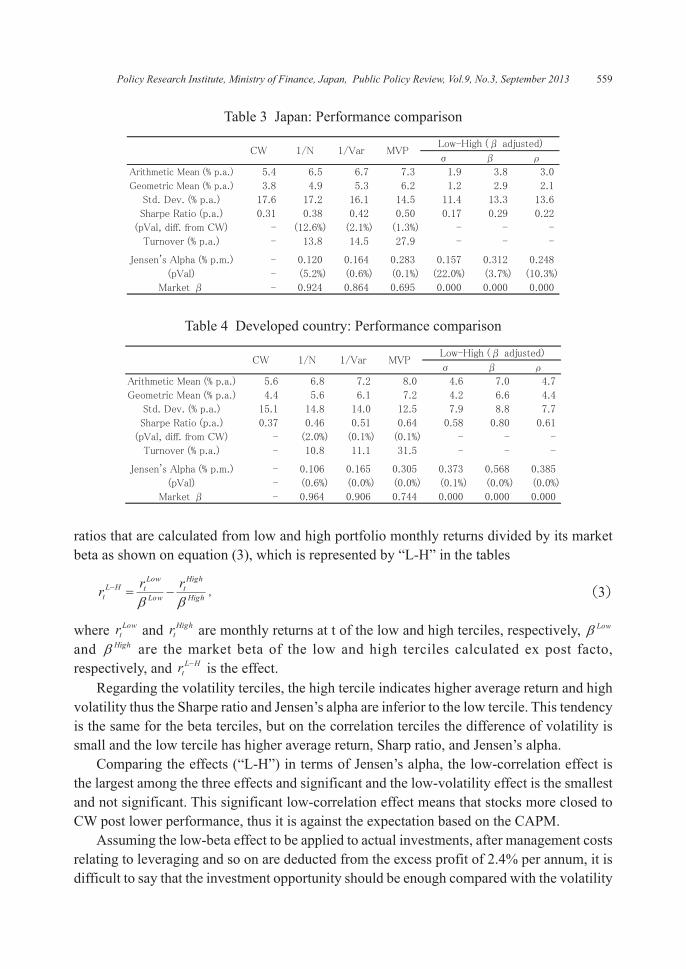
tr is the effect.Regarding the volatility terciles, the high tercile indicates higher average return and high
volatility thus the Sharpe ratio and Jensen’s alpha are inferior to the low tercile. This tendency is the same for the beta terciles, but on the correlation terciles the difference of volatility is small and the low tercile has higher average return, Sharp ratio, and Jensen’s alpha.
Comparing the effects (“L-H”) in terms of Jensen’s alpha, the low-correlation effect is the largest among the three effects and significant and the low-volatility effect is the smallest and not significant. This significant low-correlation effect means that stocks more closed to CW post lower performance, thus it is against the expectation based on the CAPM.
Assuming the low-beta effect to be applied to actual investments, after management costs relating to leveraging and so on are deducted from the excess profit of 2.4% per annum, it is difficult to say that the investment opportunity should be enough compared with the volatility
Table 3 Jap an: Performance comparison
Table 4 De vel oped country: Performance comparison
560 T Yamada / Public Policy Review
of 9.0% per annum. Thus, as mentioned earlier, in the US market the low-beta effect has existed for a long run but at least with sector indices it is confirmed not to be an anomaly that assures stable excess profits to use it actively. This is the same for the low-volatility and low-correlation effects.
Table 3 summarizes the results in the Japanese market. The test period is from January 1955 to December 2010. Here, again, we can see similar tendencies as in the US market. Compared with the US cases, MVP has much higher performance and the low-beta effect is stronger and significant, and the low-correlation effect and the low-volatility effect are a little weaker. In Japan, positive low-beta effect exists but its stability is weak as an investment opportunity.
Table 4 shows the results in the developed country market. The analysis period is from 1976 to September 2012. As the low-volatility effect and the low-correlation effect combine, the low-beta effect is very strong. This level of the effect could be enough for investment opportunity. MVP’s Jensen’s alpha reaches 3.7% per annum.
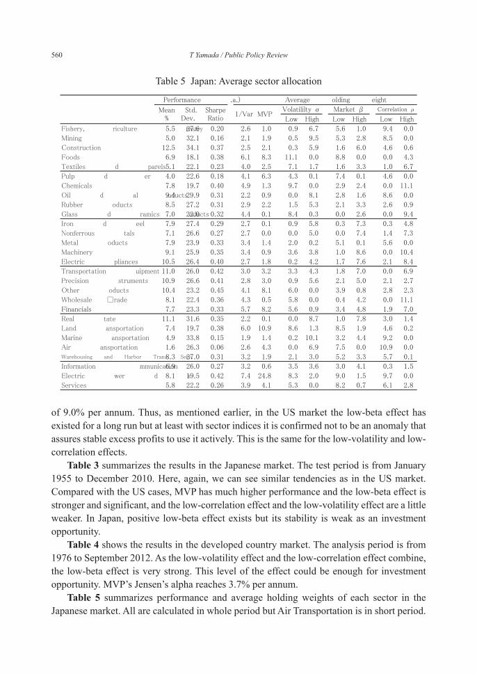
Table 5 summarizes performance and average holding weights of each sector in the Japanese market. All are calculated in whole period but Air Transportation is in short period.
Table 5 Japa n: Average sector allocation
Policy Research Institute, Ministry of Finance, Japan, Public Policy Review, Vol.9, No.3, September 2013 561
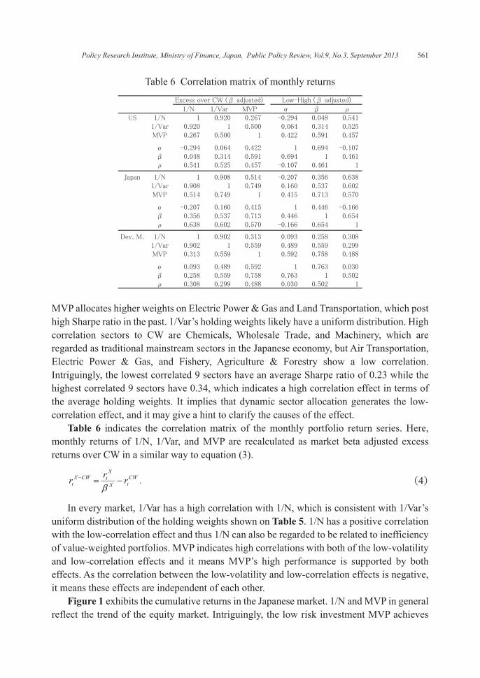
MVP allocates higher weights on Electric Power & Gas and Land Transportation, which post high Sharpe ratio in the past. 1/Var’s holding weights likely have a uniform distribution. High correlation sectors to CW are Chemicals, Wholesale Trade, and Machinery, which are regarded as traditional mainstream sectors in the Japanese economy, but Air Transportation, Electric Power & Gas, and Fishery, Agriculture & Forestry show a low correlation. Intriguingly, the lowest correlated 9 sectors have an average Sharpe ratio of 0.23 while the highest correlated 9 sectors have 0.34, which indicates a high correlation effect in terms of the average holding weights. It implies that dynamic sector allocation generates the low-correlation effect, and it may give a hint to clarify the causes of the effect.
Table 6 indicates the correlation matrix of the monthly portfolio return series. Here, monthly returns of 1/N, 1/Var, and MVP are recalculated as market beta adjusted excess returns over CW in a similar way to equation (3).
CWtX
XtCWX
t rrr (4)
In every market, 1/Var has a high correlation with 1/N, which is consistent with 1/Var’s uniform distribution of the holding weights shown on Table 5. 1/N has a positive correlation with the low-correlation effect and thus 1/N can also be regarded to be related to inefficiency of value-weighted portfolios. MVP indicates high correlations with both of the low-volatility and low-correlation effects and it means MVP’s high performance is supported by both effects. As the correlation between the low-volatility and low-correlation effects is negative, it means these effects are independent of each other.
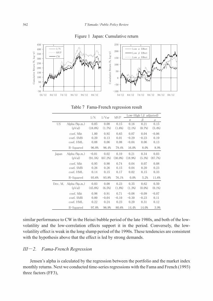
Figure 1 exhibits the cumulative returns in the Japanese market. 1/N and MVP in general reflect the trend of the equity market. Intriguingly, the low risk investment MVP achieves
Table 6 Correla t ion matrix of monthly returns
562 T Yamada / Public Policy Review
similar performance to CW in the Heisei bubble period of the late 1980s, and both of the low-volatility and the low-correlation effects support it in the period. Conversely, the low-volatility effect is weak in the long slump period of the 1990s. These tendencies are consistent with the hypothesis above that the effect is led by strong demands.
III-2. Fama-French Regression
Jensen’s alpha is calculated by the regression between the portfolio and the market index monthly returns. Next we conducted time-series regressions with the Fama and French (1993) three factors (FF3),
Table 7 Fama-French regression result
Figure 1 Japan: C umulative return
Policy Research Institute, Ministry of Finance, Japan, Public Policy Review, Vol.9, No.3, September 2013 563
tHMLt
HMLSMBt
SMBMktt
MktXt rbrbrbr (5)
where Xtr , Mkt
tr , SMBtr , and HML
tr are monthly returns at time t of the target portfolio, the market factor, the size factor (Small Minus Big), and the value factor (High Minus Low), respectively, Mktb , SMBb , and HMLb are regression loadings on each factor, and α is the intercept.
Table 7 summarizes the regression results. In the Japanese and the developed country markets, the calculation period starts from February 1970 and July 1990, respectively, because the risk factor availability is shorter than the previous analysis.
In Japan, the alphas are large in some cases, but those are not significant at the 5% level. There are positive loadings on SMB and HML, which explain almost all of the alphas. In the regression period in Japan, HML factor posts a mean return of 9.4% and standard deviation of 10.8% (per annum), which is an extremely strong anomaly compared with mean returns of 4.9% in the US and 4.4% in the developed country market.
In the US and the developed country cases, the alpha of 1/N disappears while in others significant alphas generally survive. In most regressions, the coefficients on HML are positive.
Thus, with the exception of Japanese equity, statistically significant excess returns still remain even after FF3 factor adjustment.
IV. Robustness Check
IV-1. Sector Classifications
The high performance of the ex-CW portfolios observed here can be caused because they were able to invest in the sectors that were still small but would grow larger afterwards, such as the IT industry. This issue is assumed to become more serious when more detailed classification is used.
Conversely, the railway industry in the US equity market maintained a dominant position in the past, but now this industry is seldom regarded as an independent sector. Industries that have continued to grow with high volatility form independent sector classifications, while industries whose stock prices have dropped dramatically are absorbed into other sectors. High volatility sector portfolios based on the present definition may mitigate negative influence from the latter case.
It is difficult to remove hindsight from the sector classification, but we conduct similar analysis changing the number of sectors for the US and the developed country markets. Japan is not targeted because the other sector indices except the 28 sectors are not available for the same period.
In the US, 5, 10, 17, 30 and 38 classifications are added based on the definitions of the data source. In the developed country market, 10 and 20 classifications are added.
564 T Yamada / Public Policy Review
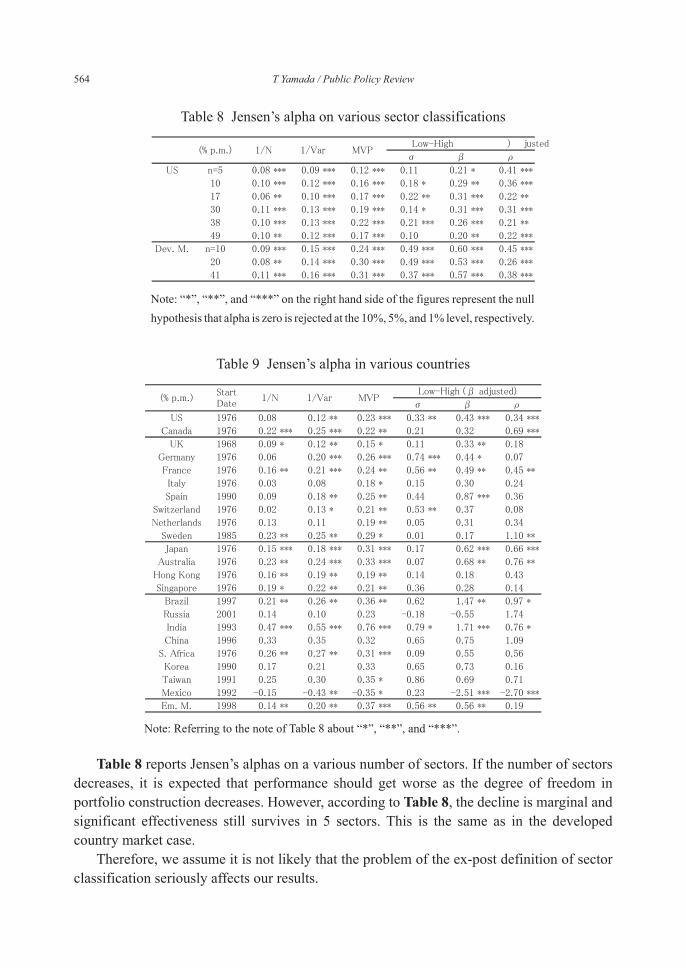
Table 8 reports Jensen’s alphas on a various number of sectors. If the number of sectors decreases, it is expected that performance should get worse as the degree of freedom in portfolio construction decreases. However, according to Table 8, the decline is marginal and significant effectiveness still survives in 5 sectors. This is the same as in the developed country market case.
Therefore, we assume it is not likely that the problem of the ex-post definition of sector classification seriously affects our results.
Table 8 Jensen’s alph a on various sector classifications
Table 9 Jensen’s alpha in various countries
Note: “*”, “**”, and “***” on the right hand side of the figures represent the null hypothesis that alpha is zero is rejected at the 10%, 5%, and 1% level, respectively.
Note: Referring to the note of Table 8 about “*”, “**”, and “***”.
Policy Research Institute, Ministry of Finance, Japan, Public Policy Review, Vol.9, No.3, September 2013 565
IV-2. Countries
We have investigated in the developed country market as well as the US and Japan so far. While the developed country market includes many countries, these two countries dominate the market in terms of market capitalization.
Then, we conducted similar analysis in various major country markets with the use of the Datastream Global Equity Index. Here, the major countries consist of the top 20 markets based on the past 10-year average of market capitalization in USD denominated at year-end on the index, plus India, Russia, and the emerging country market, thus the total number of markets becomes 23. In some countries, not all sectors are available such as Oil & Gas in Switzerland.
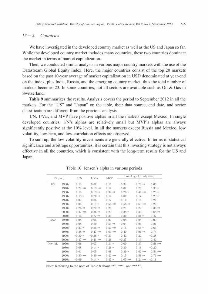
Table 9 summarizes the results. Analysis covers the period to September 2012 in all the markets. For the “US” and “Japan” on the table, their data source, end date, and sector classification are different from the previous analysis.
1/N, 1/Var, and MVP have positive alphas in all the markets except Mexico. In single developed countries, 1/N’s alphas are relatively small but MVP’s alphas are always significantly positive at the 10% level. In all the markets except Russia and Mexico, low volatility, low-beta, and low-correlation effects are observed.
To sum up, the low volatility investments are generally effective. In terms of statistical significance and arbitrage opportunities, it is certain that this investing strategy is not always effective in all the countries, which is consistent with the long-term results for the US and Japan.
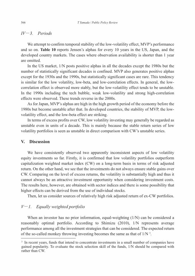
Table 10 Jensen’s alpha i n various periods
Note: Referring to the note of Table 8 about “*”, “**”, and “***”.
566 T Yamada / Public Policy Review
IV-3. Periods
We attempt to confirm temporal stability of the low-volatility effect, MVP’s performance and so on. Table 10 reports Jensen’s alphas for every 10 years in the US, Japan, and the developed country markets. The cases where observation availability is shorter than 1 year are omitted.
In the US market, 1/N posts positive alphas in all the decades except the 1980s but the number of statistically significant decades is confined. MVP also generates positive alphas except for the 1930s and the 1990s, but statistically significant cases are rare. This tendency is similar for the low volatility, low-beta, and low-correlation effects. In general, the low-correlation effect is observed more stably, but the low-volatility effect tends to be unstable. In the 1990s including the tech bubble, weak low-volatility and strong high-correlation effects were observed. These trends reverse in the 2000s.
As for Japan, MVP’s alphas are high in the high growth period of the economy before the 1980s but become unstable after that. In developed countries, the stability of MVP, the low-volatility effect, and the low-beta effect are striking.
In terms of excess profits over CW, low volatility investing may generally be regarded as unstable even in units of a decade. This is mainly because the stable return series of low volatility portfolios is seen as unstable in direct comparison with CW’s unstable series.
V. Discussion
We have consistently observed two apparently inconsistent aspects of low volatility equity investments so far. Firstly, it is confirmed that low volatility portfolios outperform capitalization weighted market index (CW) on a long-term basis in terms of risk adjusted return. On the other hand, we see that the investments do not always ensure stable gains over CW. Comparing on the level of excess returns, the volatility is substantially high and thus it cannot always be an attractive investment opportunity when considering investment costs. The results here, however, are obtained with sector indices and there is some possibility that higher effects can be derived from the use of individual stocks.
Then, let us consider sources of relatively high risk adjusted return of ex-CW portfolios.
V-1. Equally weighted portfolio
When an investor has no prior information, equal-weighting (1/N) can be considered a reasonably optimal portfolio. According to Shimizu (2010), 1/N represents average performance among all the investment strategies that can be considered. The expected return of the so-called monkey throwing investing becomes the same as that of 1/N 3.
3 In recent years, funds that intend to concentrate investments in a small number of companies have gained popularity. To evaluate the stock selection skill of the funds, 1/N should be compared with rather than CW.
Policy Research Institute, Ministry of Finance, Japan, Public Policy Review, Vol.9, No.3, September 2013 567
In real markets, it is well-known that 1/N outperforms CW. For example, DeMiguel et al. (2009) reports that 1/N indicates superior performance to CW and other investment strategies in broad universes besides equity. Hamza et al. (2007) indicates 1/N portfolio composed of developed country indices has a higher Sharpe ratio than CW and GDP weighted portfolios. Chow et al. (2011) and Yamada (2012) report 1/N’s performance is similar to the fundamental weighted portfolio proposed by Arnott et al. (2005).
As 1/N investments do not require any theories or any special information, these are inconvenient results for the asset management industry.
On the other hand, several problems of 1/N are pointed out in applying to real investments. Comparing with CW, say, 1/N necessarily tends to invest too much in small-cap assets and thus its manageable amount limit should be low, to require high portfolio turnover, and so on. However, Zeng et al. (2010) conclude that these problems are rather exaggerated based on their real experience of the S&P500 constituent 1/N index over 7 years. In addition, our investigation methods and results likely suggest 1/N has enough superiority even when considering these issues.
According to the analysis in Plyakha et al. (2012), 1/N’s superior performance to CW is explained by the exposures to the FF3 factors and the idiosyncratic part. The latter stems from the portfolio’s monthly rebalancing and consists of reversals, idiosyncratic volatilities, and the lead-lag characteristics of individual stock prices. In our paper, we use sector indices and the rebalance interval is longer, so the latter is assumed to be negligible. As for the former, Table 7 indicates the value stock effect as well as the small-cap effect explaining 1/N’s performance. However, it is not easy to intuitively understand that the difference between 1/N and CW is related to value stocks.
Treynor (2005) insists that CW portfolio depends on market prices and tends to overweight the stocks that are overvalued and underweight the stocks that are undervalued. Because we do not know the real value of a stock, he points out that a portfolio, such as 1/N, that does not depend on market prices can generate a higher return. Under his argument, 1/N can be explained by the value investing standpoint that focuses on the comparison of the current price to a real enterprise value.
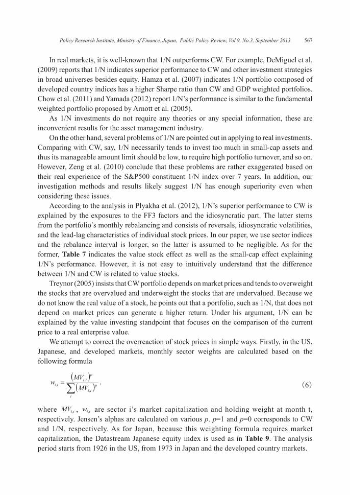
We attempt to correct the overreaction of stock prices in simple ways. Firstly, in the US, Japanese, and developed markets, monthly sector weights are calculated based on the following formula
i
pti
pti
ti MVMV
w,
,, (6)
where tiMV , , tiw , are sector i’s market capitalization and holding weight at month t, respectively. Jensen’s alphas are calculated on various p. p=1 and p=0 corresponds to CW and 1/N, respectively. As for Japan, because this weighting formula requires market capitalization, the Datastream Japanese equity index is used as in Table 9. The analysis period starts from 1926 in the US, from 1973 in Japan and the developed country markets.
568 T Yamada / Public Policy Review
The results are shown on Figure 2. In the figure, there are good news and bad news for CW. The bad news is that relaxing the overreaction of stock prices (p<1) enables the generation of positive alphas. The good news is that since there is a monotonically decreasing relationship between p and performance, it implies that some risk premium related to p exists and does not imply an own drawback to CW.
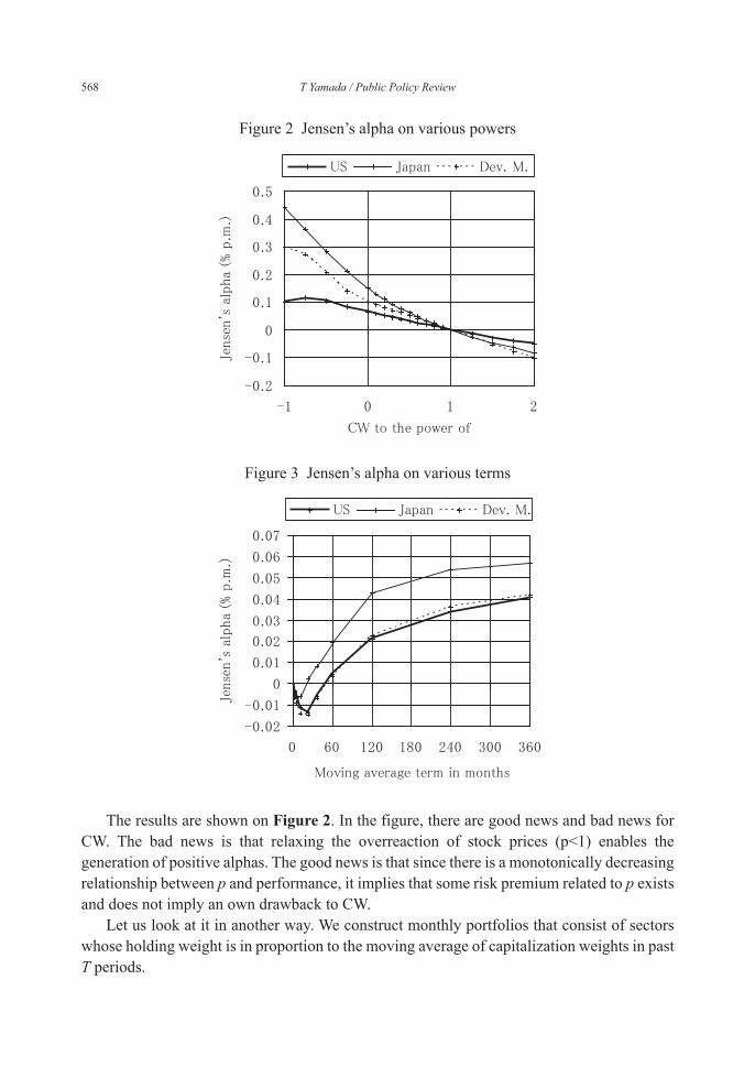
Let us look at it in another way. We construct monthly portfolios that consist of sectors whose holding weight is in proportion to the moving average of capitalization weights in past T periods.
Figure 2 Jensen’s alpha o n various powers
Figure 3 Jensen’s alpha on va rious terms
Policy Research Institute, Ministry of Finance, Japan, Public Policy Review, Vol.9, No.3, September 2013 569
1
0 ,
,,
1 T
iti
titi MV
MVT
w (7)
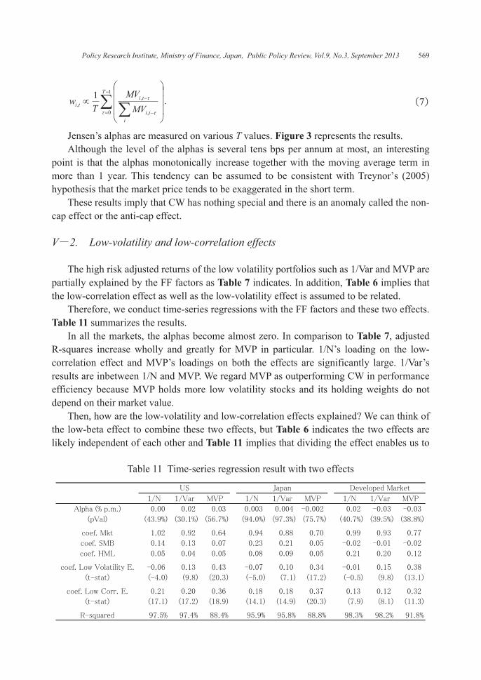
Jensen’s alphas are measured on various T values. Figure 3 represents the results.Although the level of the alphas is several tens bps per annum at most, an interesting
point is that the alphas monotonically increase together with the moving average term in more than 1 year. This tendency can be assumed to be consistent with Treynorʼs (2005) hypothesis that the market price tends to be exaggerated in the short term.
These results imply that CW has nothing special and there is an anomaly called the non-cap effect or the anti-cap effect.
V-2. Low-volatility and low-correlation effects
The high risk adjusted returns of the low volatility portfolios such as 1/Var and MVP are partially explained by the FF factors as Table 7 indicates. In addition, Table 6 implies that the low-correlation effect as well as the low-volatility effect is assumed to be related.
Therefore, we conduct time-series regressions with the FF factors and these two effects. Table 11 summarizes the results.
In all the markets, the alphas become almost zero. In comparison to Table 7, adjusted R-squares increase wholly and greatly for MVP in particular. 1/N’s loading on the low-correlation effect and MVP’s loadings on both the effects are significantly large. 1/Var’s results are inbetween 1/N and MVP. We regard MVP as outperforming CW in performance efficiency because MVP holds more low volatility stocks and its holding weights do not depend on their market value.
Then, how are the low-volatility and low-correlation effects explained? We can think of the low-beta effect to combine these two effects, but Table 6 indicates the two effects are likely independent of each other and Table 11 implies that dividing the effect enables us to
Table 11 Time-series regressio n result with two effects
570 T Yamada / Public Policy Review
capture the sources of 1/N and MVP from two sides4.As for the low-volatility effect, in the hypothesis described above, excess demands for
high risk assets should be applied when borrowing is restricted. It is consistent with the results in Yamada and Nagawatari (2010) and Hsu et al. (2013) that high volatility stocks tend to be overestimated in earnings forecasts and to be overpriced.
If CW becomes inefficient because of the low-volatility effect, equation (2) implies the low-correlation effect can simply attend on it. However, this explanation is inconsistent with the fact that both the effects are roughly independent temporally in Table 6.
Assuming that the low correlation and value stock effects have the same origin, the hypothesis for the value stock effect can be applied. It will be a future problem to make the anomalies that would be caused by overvalued stock prices consistent, such as the low-correlation, small-cap, and value stock effects and the difference between 1/N and CW.
VI. Conclusion
We verify long-term performance of the low volatility investment in the world stock markets. As a result, we confirm robust low volatility, low-beta, and low-correlation effects, and that low volatility portfolios such as the global minimum variance portfolio (MVP) indicate superior risk adjusted return to the market capitalization weighted indices (CW). In addition, the low-volatility and low-correlation effects play an importance role in explaining excess performance.
However, it is difficult to conclude that these effects can stably generate excess profits by themselves, and thus they do not really amount to counterevidence for market equilibrium.
They rather pose a question for the CW centric performance evaluation system that dominates the current asset management industry. In this world, CW is generally assumed to be the highest Sharpe ratio portfolio by the CAPM and the strategies that try to lower the tracking error and raise the excess return over CW are highly evaluated. Our results show, however, that it is difficult to justify the expectation even approximately that the Sharpe ratio of CW is the highest. Premising this reality, investors should think of how to manage and evaluate their portfolios under their primary purposes.
Fama and French (2004) point out that investing in the low-beta, small-cap, and value stocks tend to generate superior performance to CW without special skills. Now the small-cap and value stock investments have been established as styles of equity investments. To help and occasionally replace market capitalization weighted indices, the low beta or low volatility equity investments also seem sufficient to become popular in the future.
4 Applying the same regression on the Maximum Diversification portfolio introduced by Choueifaty and Coignard (2008), it is shown that the low-volatility effect has almost no relation but the low correlation effect has a strong relation with the performance.
Policy Research Institute, Ministry of Finance, Japan, Public Policy Review, Vol.9, No.3, September 2013 571
VII. Appendix
VII-1. Construction of the minimum variance portfolio
Generally the minimum variance portfolio is constructed with the covariance matrix of the assets. Here, how to estimate the covariance matrix is a problem. It is known that the sample covariance matrix computed with historical asset returns likely causes substantial estimation errors in cases where there are not enough periods much larger than the number of assets.
We use the Bayesian Shrinkage method to solve it. The basic idea behind it is to shrink the sample matrix to a prior estimation estimated by some assumption instead of using the matrix as it stands.
Concretely, the covariance matrix used on portfolio construction is defined by a weighted average of the sample matrix S and the prior matrix F,
SF 1 (8)
where is a shrinkage coefficient and is determined to increase when the uncertainty of S increases.
We assert a prior estimation matrix F that is composed of identical variances and identical correlation coefficients. The former are the average of all the variances, that is, the average of all the diagonal components of the covariance matrix. The latter are the average of all the pairwise correlation coefficients, that is, the average of all the non-diagonal components. That is, the averages are defined by:
N
iiisN
s1
1 , 1
1 112 N
i
N
ijijrNN
r , (9)
where N is the number of assets, ijs is a component of the sample matrix S, and ijr is a correlation coefficient.
Referring to Ledoit and Wolf (2004), an optimal shrinkage coefficient ˆ is estimated by:
ˆˆˆ1ˆ
T, (10)
N
i
N
j
T
tijjjtiit syyyy
T1 1 1
21ˆN
i
N
jijij sf
1 1
2ˆ (11)
where T is the number of observations, ity is a return of asset i at t, iy is the average return of asset I, and ijf is a component of the prior estimation matrix F.
Since our F is not the same as that of Ledoit and Wolf (2004), ˆ is also in a different form. By definition:
572 T Yamada / Public Policy Review
N
i
N
jji jisT Tf
1 1
,AsyCov (12)
Ignoring estimation errors in r and ˆ of the sample matrix, ˆ can be estimated by the sum of diagonal and non-diagonal component parts.
ODD ˆˆˆ (13)
N
iii
N
k
T
tiitkktD ssyyyy
NT1 1 1
221ˆ (14)
N
i
N
jij
N
k
T
tjjtiitkktOD ssyyyyyy
NTr
1 1 1 1
21ˆ (15)
In reality, ˆ ’s minimum, maximum, and m edian in the whole period are 0.101, 0.774, and 0.194 in the US; 0.153, 0.402, and 0.230 in Japan; and 0.134, 0.596, and 0.321 in the developed country market, respectively. In general, a higher weight is allocated on the sample covariance matrix.
VII-2. Arithmetic and geometric means
In our paper, the arithmetic and geometric means are displayed as averages of monthly returns. If asset prices are in geometric Brownian motion, the relationship between the means is expected as follows:
2
21
AG (16)
where G is the geometric mean, A is the arithmetic mean, and is a volatility.In case of high volatility assets such as stocks, the difference between the arithmetic and
geometric means can become unexpectedly large. For example, assuming two stocks whose volatiles are 15% and 25% per annum, the second term of the right hand side in equation (16) is 1.1% and 3.1%, respectively. If the arithmetic means of the stocks are identical, the geometric means differ by 2% per annum. In fact, the definition of the mean substantially affects the level of the volatility effect and its statistical significance.
In our paper, the arithmetic mean is generally used because this is a more conservative measure for the low-volatility effect, but there are many arguments in which mean is more exact as an estimation of the expected return.
If we know the exact mean and variance moments of the distribution of future returns, the arithmetic mean is theoretically the precise estimation. In reality, however, it is unavoidable that some estimation errors occur in the two parameters.
Blume (1974) points out that the estimation errors may incur an overestimation tendency in the arithmetic mean. As the estimation error occurred in the mean is generally in proportion
Policy Research Institute, Ministry of Finance, Japan, Public Policy Review, Vol.9, No.3, September 2013 573
to the variance of the returns, the geometric mean that gives a penalty on the variance can become a more precise expected return than the arithmetic one as a result. According to Jacquier et al. (2005), the comparison depends on the size of the estimation error, and the arithmetic mean is more precise in cases where the error is small, and the geometric mean or the measure with a higher penalty on variance is more precise in cases where the error is large.
References
Arnott, R. D., J. C. Hsu, and P. Moore (2005), “Fundamental Indexation,” Financial Analysts Journal, Vol. 61 No. 2, pp. 83-99
Black, F. (1972), “Capital market equilibrium with restricted borrowing,” Journal of Business, Vol. 45 No. 3, pp. 444-455
Black, F., M.C. Jensen, and M. Scholes (1972), “The Capital Asset Pricing Model: Some Empirical Tests,” in M. Jensen (ed), Studies in the Theory of Capital Markets, New York, Praeger
Blitz, D. C. and P. van Vliet (2007), “The Volatility Effect,” Journal of Portfolio Management, Vol. 34 No. 1, pp. 102-113
Blume, J. (1974), “Unbiased Estimators of Long-Run Expected Rates of Return,” Journal of the American Statistical Association, Vol. 69 No. 347, pp. 634-638
Choueifaty, Y. and Y. Coignard (2008), “Toward Maximum Diversification,” Journal of Portfolio Management, Vol. 35 No. 1, pp. 40-51
Chow, T., J. Hsu, V. Kalesnik, and B. Little (2011), “A Survey of Alternative Equity Index Strategies,” Financial Analysts Journal, Vol. 67 No 5, pp. 37-57
Clarke, R. G., H. de Silva, and S. Thorley (2006), “Minimum-Variance Portfolios in the U.S. Equity Market,” Journal of Portfolio Management, Vol. 33 No. 1, pp. 10-24
DeMiguel, V., L. Garlappi, and R. Uppal (2007), “Optimal versus naive diversification: How inefficient is the 1/N portfolio strategy?,” Review of Financial Studies, Vol. 22 No. 5, pp. 1915-1953
Fama, E. F. and K. R. French (1993), “Common Risk Factors in the Returns on Stocks and Bonds,” Journal of Financial Economics, Vol. 33 No. 1, pp. 3-56
Fama, E. F. and K. R. French (2004), “The Capital Asset Pricing Model: Theory and Evidence,” Journal of Economic Perspectives, Vol. 18 No. 3, pp. 25-46
Frazzini, A. and L. H. Pedersen (2010), “Betting against Beta,” Working PaperHamza, O., M. Kortas, J. F. L'Her, and M. Roberge (2007), “International Equity Indices:
Exploring Alternatives to Market Cap-Weighting,” Journal of Investing, Vol. 16 No. 2, pp. 103-118
Haugen, R. A. and N. L. Baker (1991), “The Efficient Market Inefficiency of Capitalization-Weighted Stock Portfolios,” Journal of Portfolio Management, Vol. 17 No. 3, pp. 35-40
Honda, T. and K. Takahashi (2011), “Reconsideration of Equity Index-Reducing risk through index diversification-,” Securities Analysts Journal, Vol. 49 No. 12, pp. 91-101
574 T Yamada / Public Policy Review
Hsu, J., H. Kudoh, and T. Yamada (2013), “When Sell-Side Analysts Meet High-Volatility Stocks: An Alternative Explanation for the Low-Volatility Puzzle,” Journal of Investment Management, forthcoming
Jacquier, E., A. Kane, and A. J. Marcus (2005), “Optimal Estimation of the Risk Premium for the Long Run and Asset Allocation: A Case of Compounded Estimation Risk,” Journal of Financial Econometrics, Vol. 3 No. 1, pp. 37-55
Ledoit, O. and M. Wolf (2003), “Honey, I Shrunk the Sample Covariance Matrix,” Journal of Portfolio Management, Vol. 31 No. 1
Markowitz, H. M. (2005), “Market Efficiency: A Theoretical Distinction and so What?,” Financial Analysts Journal, Vol. 61 No. 5, pp. 17-30
Mehrling, P. (2005), Fischer Black and the Revolutionary Idea of Finance, WileyPlyakha, Y., R. Uppal, and G. Vilkov (2012), “Why Does an Equal-Weighted Portfolio
Outperform Value- and Price-Weighted Portfolios?,” Working PaperSharpe, W. F. (1991), “Capital Asset Prices with and without Negative Holdings,” Journal of
Finance, Vol. 46 No. 2, pp. 489-509Shimizu, M. (2010), “Equally Weighted Rebalancing as the Average of all Investment
Strategies,” Journal of Investment Management, Vol. 8 No. 4Treynor, J. (2005), “Why Market-Valuation-Indifferent Indexing Works,” Financial Analysts
Journal, Vol. 61 No. 5Yamada, T. (2012), “Reconsideration of Equity portfolios,” Fund Management, summer, pp.
6-11Yamada, T. and M. Nagawatari (2010), “Investor Expectations and the Volatility Puzzle in
the Japanese Stock Market,” Securities Analysts Journal, Vol. 48 No. 12, pp. 47-57Yamada, T. and I. Uesaki (2009), “Low Volatility Strategy in Global Equity Markets,”
Securities Analysts Journal, Vol. 47 No. 6, pp. 97-110Zeng, L., S. Dash, and D. Guarino (2010), “Equal Weight Indexing - Seven Years Later,”
Standard & Poor's
Related Documents