Long-term tidal level distribution using a wave-by-wave approach

www.elsevier.com/locate/advwatres

Advances in Water Resources 30 (2007) 2271–2282

Long-term tidal level distribution using a wave-by-wave approach

Sonia Castanedo *, Fernando J. Mendez, Raul Medina, Ana J. Abascal

Ocean and Coastal Research Group, IH Cantabria, Universidad de Cantabria. Avda. de los Castros s/n. 39005, Santander, Spain

Received 28 November 2006; received in revised form 3 May 2007; accepted 7 May 2007Available online 21 May 2007

Abstract

Tidal analysis is usually performed in the time domain by means of the decomposition of the time series of the free surface in a numberof harmonics, characterizing every single component along a shelf or inside an estuary. Although this kind of analysis has proven to bevery useful in numerous studies, when it comes to characterizing the tide statistically (i.e., the long-term sea level distribution) thisapproach is inadequate. This paper presents a different approach. Instead of working with the complete time series, some statistical prop-erties of the signal, such as the probability density function (pdf) of the tidal wave heights (TWH) are used. The tidal elevation (TE) pdf isobtained by means of a statistical procedure that consists of the definition of the compound pdf as a function of the TWH pdf and the U-shaped pdf for the elevations of a single wave. In order to have an analytical representation of the probability density functions, the useof kernel density functions is explored. An extension to account for asymmetries in the tidal elevations is also proposed. Both, the sym-metric and the asymmetric models are applied to different tide gauge data along the World’s coastline (symmetric and asymmetric – posi-tive and negative skewed –). The results show that the symmetric approach is capable of representing the TE pdfs for roughly symmetrictides. However, in shallow areas where the distortion of the tide is more pronounced, the asymmetric model provides a better descriptionof the TE pdfs.� 2007 Elsevier Ltd. All rights reserved.

Keywords: Tidal elevation; Tidal range; Statistical analysis; Tidal asymmetry; Nodal cycle; Probability density function; Kernel density model

1. Introduction

Knowledge of sea level fluctuations in a bay or estuaryhas been the key stone of many scientific studies and estu-arine restoration and protection projects. Designing achannel entrance with navigation criteria, establishingflood defences, preventing shoreline erosion and, in gen-eral, any man-made alterations to these systems requirethe determination of sea level. Sea level analysis in tidaldominated embayments, has traditionally been performedthrough the calculation and prediction of tides andcurrents. Usually, this has been done decomposing atidal record into a number of harmonics constituents

0309-1708/$ - see front matter � 2007 Elsevier Ltd. All rights reserved.

doi:10.1016/j.advwatres.2007.05.005

* Corresponding author. Tel.: +34 942 201810; fax: +34 942 20 18 60.E-mail addresses: [email protected] (S. Castanedo), mendezf@

unican.es (F.J. Mendez), [email protected] (R. Medina), [email protected] (A.J. Abascal).

[7,3,6,8,12,24]. However, the study of tidal records from astatistical point of view is increasingly used in differentapplications.

Due to the increasing awareness of the ecological impor-tance of wetlands and coastal aquifers, environmental stud-ies, guidelines or even political strategies aimed at therestoration of these usually degraded habitats, are beingdeveloped in several countries [4,25,17,14,13]. Frequencyand duration of flooding or soil saturation, water perma-nence and water regime are key factors in describing thehydrology of these systems [22,15].

Moreover, studies of extreme water levels using the jointprobability of surge and tide require a proper determina-tion of the probabilistic distribution of tidal elevations.Also, the importance of tidal asymmetries in the transportand accumulation of sediments in estuaries demands a sta-tistical study of tide. Accordingly, the probability densityfunction (pdf) of the tidal elevation (hereafter, TE) is

mailto:[email protected]






2272 S. Castanedo et al. / Advances in Water Resources 30 (2007) 2271–2282

increasingly used to statistically describe the tide at a spe-cific location [23,19,26].

In this paper, the statistical distribution of tidal levels,hereafter also named long-term water level distribution, isexamined in more detail. A statistical approach is presentedto be applied in the study of areas with predominantlysemidiurnal tides. The novelty here is that, instead of work-ing with the complete time series, we will make use of somestatistical properties of the signal. The main assumption isthat a free surface tidal record can be represented as a con-secutive series of waves with different wave heights (tidalrange) and wave periods (tidal period). Therefore, althoughthe time scales are very different, a parallelism between theshort-term probabilistic description of the free surface in asea state (1 h) and the analysis of a tidal record (years) isexplored.

2. Tide gauge data

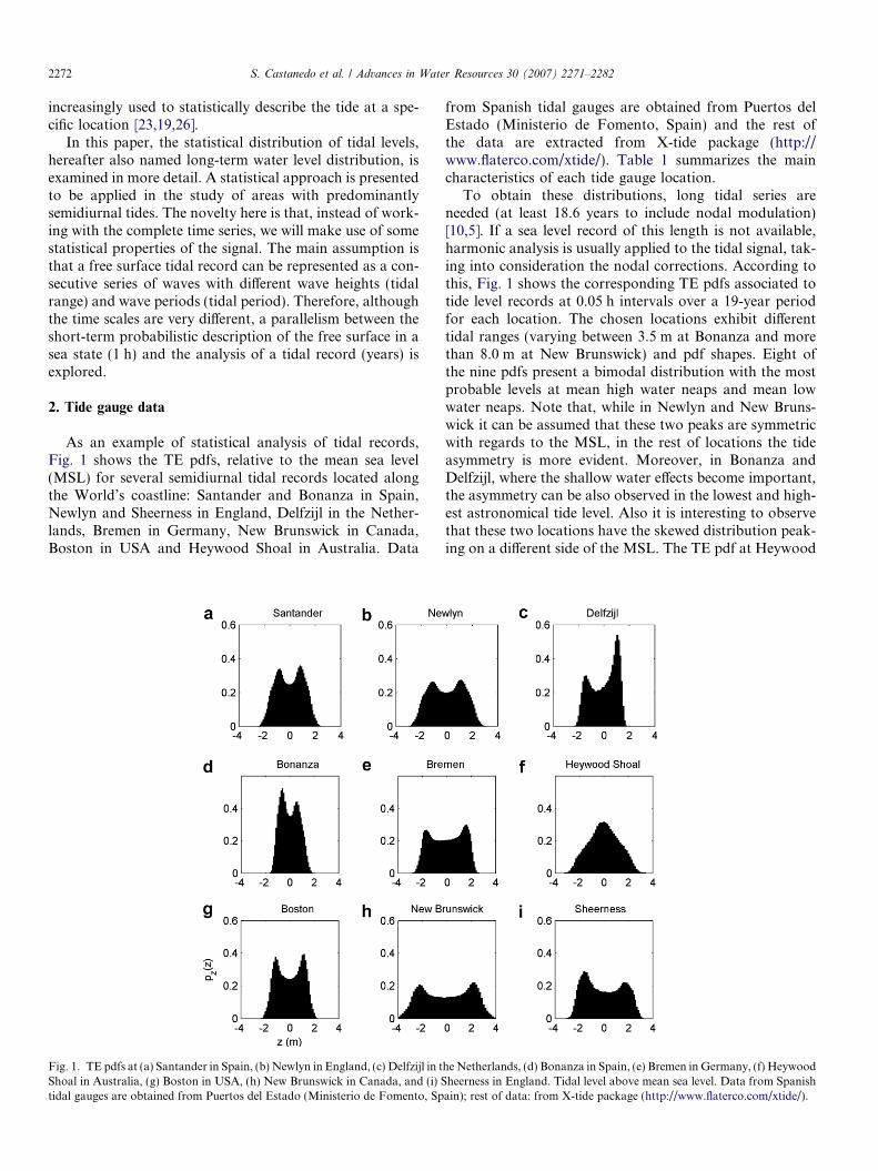
As an example of statistical analysis of tidal records,Fig. 1 shows the TE pdfs, relative to the mean sea level(MSL) for several semidiurnal tidal records located alongthe World’s coastline: Santander and Bonanza in Spain,Newlyn and Sheerness in England, Delfzijl in the Nether-lands, Bremen in Germany, New Brunswick in Canada,Boston in USA and Heywood Shoal in Australia. Data

Fig. 1. TE pdfs at (a) Santander in Spain, (b) Newlyn in England, (c) Delfzijl in tShoal in Australia, (g) Boston in USA, (h) New Brunswick in Canada, and (i) Stidal gauges are obtained from Puertos del Estado (Ministerio de Fomento, Sp

from Spanish tidal gauges are obtained from Puertos delEstado (Ministerio de Fomento, Spain) and the rest ofthe data are extracted from X-tide package (http://www.flaterco.com/xtide/). Table 1 summarizes the maincharacteristics of each tide gauge location.

To obtain these distributions, long tidal series areneeded (at least 18.6 years to include nodal modulation)[10,5]. If a sea level record of this length is not available,harmonic analysis is usually applied to the tidal signal, tak-ing into consideration the nodal corrections. According tothis, Fig. 1 shows the corresponding TE pdfs associated totide level records at 0.05 h intervals over a 19-year periodfor each location. The chosen locations exhibit differenttidal ranges (varying between 3.5 m at Bonanza and morethan 8.0 m at New Brunswick) and pdf shapes. Eight ofthe nine pdfs present a bimodal distribution with the mostprobable levels at mean high water neaps and mean lowwater neaps. Note that, while in Newlyn and New Bruns-wick it can be assumed that these two peaks are symmetricwith regards to the MSL, in the rest of locations the tideasymmetry is more evident. Moreover, in Bonanza andDelfzijl, where the shallow water effects become important,the asymmetry can be also observed in the lowest and high-est astronomical tide level. Also it is interesting to observethat these two locations have the skewed distribution peak-ing on a different side of the MSL. The TE pdf at Heywood

he Netherlands, (d) Bonanza in Spain, (e) Bremen in Germany, (f) Heywoodheerness in England. Tidal level above mean sea level. Data from Spanish

ain); rest of data: from X-tide package (http://www.flaterco.com/xtide/).

http://www.flaterco.com/xtide/



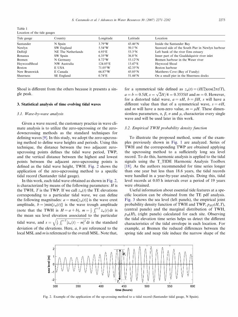
Table 1Location of the tide gauges

Tide gauge Country Longitude Latitude Location

Santander N Spain 3.79�W 43.46�N Inside the Santander BayNewlyn SW England 5.54�W 50.1�N Seaward side of the South Pier in Newlyn harbourDelfzijl NE The Netherlands 6.93�E 53.3�N Left bank of the river Ems estuaryBonanza SW Spain 6.35�W 36.8�N Inner part of the Gualdalquivir river inletBremen N Germany 8.72�W 53.12�N Bremen harbour in the Weser riverHeywoodShoal NW Australia 124.05�E 13.47�S Heywood ShoalBoston E USA 71.05�W 42.35�N Boston harbourNew Brunswick E Canada 66.87�W 45.05�N Matthews Cove (Bay of Fundy)Sheerness SE England 0.74�E 51.44�N On a small pier in the Sheerness docks

S. Castanedo et al. / Advances in Water Resources 30 (2007) 2271–2282 2273

Shoal is different from the others because it presents a sin-gle peak.

3. Statistical analysis of time evolving tidal waves

3.1. Wave-by-wave analysis

Given a wave record, the customary practice in wave cli-mate analysis is to utilize the zero-upcrossing or the zero-downcrossing methods as the standard techniques fordefining waves [9]. In this study, we adopt the zero-upcross-ing method to define wave heights and periods. Using thistechnique, the distance between the two adjacent zero-upcrossing points defines the tidal wave period, TWP,and the vertical distance between the highest and lowestpoints between the adjacent zero-upcrossing points isdefined as the tidal wave height, TWH. Fig. 2 shows theapplication of the zero-upcrossing method to a specifictidal record (Santander tidal gauge).

In this work, each tidal wave obtained as shown in Fig. 2,is characterized by means of the following parameters: H isthe TWH, T is the TWP. If we call zw(t) the TE elevationscorresponding to a particular tidal wave, we can definethe following magnitudes: a = max[zw(t)] is the wave crestamplitude, b = jmin[zw(t)]j is the wave trough amplitude

(note that the TWH is H = a + b), m ¼ 1T

R tþTt zwðtÞdt is

the mean sea level elevation associated to the particular

tidal wave, and s ¼ffiffiffiffiffiffiffiffiffiffiffiffiffiffiffiffiffiffiffiffiffiffiffiffiffiffiffiffiffiffiffiffiffiffiffiffiffiffiffiffiffi1T

R tþTt ½zwðtÞ � m�2 dt

qis the standard

deviation of the elevations. Here, a, b are referenced to thelocal MSL and m is referenced to the overall MSL. Note that,

Fig. 2. Example of the application of the up-crossing meth

for a symmetrical tide defined as zw(t) = (H/2)cos(2pt/T),

a = b = 0.5H, s ¼ffiffiffi2p

H=4 ¼ 0:3535H and m = 0. However,for a distorted tidal wave, a = aH, b = bH, s will have adifferent value than that of a symmetrical wave, s = rH,and m will have a non-zero value, m = lH. These dimen-sionless parameters, a, b, r and l, characterize every singlewave and will be used later in this work.

3.2. Empirical TWH probability density function

To illustrate the proposed method, some of the exam-ples previously shown in Fig. 1 are analyzed. Series ofTWH and the corresponding TWP are obtained applyingthe upcrossing method to a sufficiently long sea levelrecord. To do this, harmonic analysis is applied to the tidalsignals using the T_TIDE Harmonic Analysis Toolbox[18]. As the authors recommended for time series longerthan one year but less than 18.6 years, the tidal recordswere handled in a year-by-year analysis. Doing this, tidallevel records at 0.05 h intervals over a period of 19 yearswere obtained.

Useful information about essential tide features at a spe-cific location can be obtained from the TE pdf analysis.Fig. 3 shows the sea level (left panels), the empirical jointprobability density function of TWH and TWP, pHT(H,T),(central panels) and the marginal distribution of TWH,pH(H), (right panels) calculated for each site. Observingthe tidal elevation time series helps us detect the differentcharacteristics of the tidal envelope in each location. Forexample, at Bremen the reduced differences between thespring tide and neap tide induce the narrow shape of the

od to a tidal record (Santander tidal gauge, N Spain).

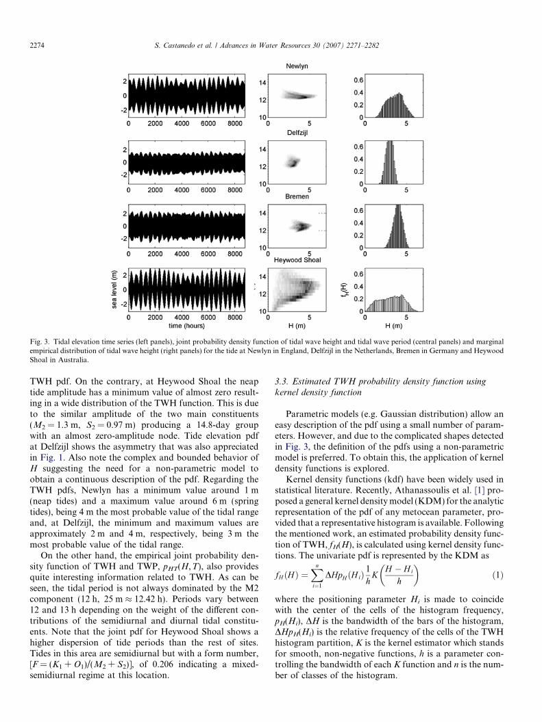
Fig. 3. Tidal elevation time series (left panels), joint probability density function of tidal wave height and tidal wave period (central panels) and marginalempirical distribution of tidal wave height (right panels) for the tide at Newlyn in England, Delfzijl in the Netherlands, Bremen in Germany and HeywoodShoal in Australia.


TWH pdf. On the contrary, at Heywood Shoal the neaptide amplitude has a minimum value of almost zero result-ing in a wide distribution of the TWH function. This is dueto the similar amplitude of the two main constituents(M2 = 1.3 m, S2 = 0.97 m) producing a 14.8-day groupwith an almost zero-amplitude node. Tide elevation pdfat Delfzijl shows the asymmetry that was also appreciatedin Fig. 1. Also note the complex and bounded behavior ofH suggesting the need for a non-parametric model toobtain a continuous description of the pdf. Regarding theTWH pdfs, Newlyn has a minimum value around 1 m(neap tides) and a maximum value around 6 m (springtides), being 4 m the most probable value of the tidal rangeand, at Delfzijl, the minimum and maximum values areapproximately 2 m and 4 m, respectively, being 3 m themost probable value of the tidal range.

On the other hand, the empirical joint probability den-sity function of TWH and TWP, pHT(H,T), also providesquite interesting information related to TWH. As can beseen, the tidal period is not always dominated by the M2component (12 h, 25 m � 12.42 h). Periods vary between12 and 13 h depending on the weight of the different con-tributions of the semidiurnal and diurnal tidal constitu-ents. Note that the joint pdf for Heywood Shoal shows ahigher dispersion of tide periods than the rest of sites.Tides in this area are semidiurnal but with a form number,[F = (K1 + O1)/(M2 + S2)], of 0.206 indicating a mixed-semidiurnal regime at this location.

3.3. Estimated TWH probability density function using

kernel density function

Parametric models (e.g. Gaussian distribution) allow aneasy description of the pdf using a small number of param-eters. However, and due to the complicated shapes detectedin Fig. 3, the definition of the pdfs using a non-parametricmodel is preferred. To obtain this, the application of kerneldensity functions is explored.

Kernel density functions (kdf) have been widely used instatistical literature. Recently, Athanassoulis et al. [1] pro-posed a general kernel density model (KDM) for the analyticrepresentation of the pdf of any metocean parameter, pro-vided that a representative histogram is available. Followingthe mentioned work, an estimated probability density func-tion of TWH, fH(H), is calculated using kernel density func-tions. The univariate pdf is represented by the KDM as

fH ðHÞ ¼Xn

i¼1

DHpH ðH iÞ1

hK

H � H i

h

� �ð1Þ

where the positioning parameter Hi is made to coincidewith the center of the cells of the histogram frequency,pH(Hi), DH is the bandwidth of the bars of the histogram,DHpH(Hi) is the relative frequency of the cells of the TWHhistogram partition, K is the kernel estimator which standsfor smooth, non-negative functions, h is a parameter con-trolling the bandwidth of each K function and n is the num-ber of classes of the histogram.


Martinez and Martinez [16] discuss the efficiency ofseveral kernels and they conclude that the choice of a ker-nel depends on computational considerations or on theamount of differentiability required in the estimate. Fol-lowing this, in this work the triweight kernel has beenused

KðxÞ ¼3532ð1� x2Þ3 jxj 6 1

0 jxj > 1

(ð2Þ

Similar results were obtained using the triangular or the bi-weight kernels. It is important to note that these kernels areleft and right bounded, which is an important requirementof the TWH distribution.

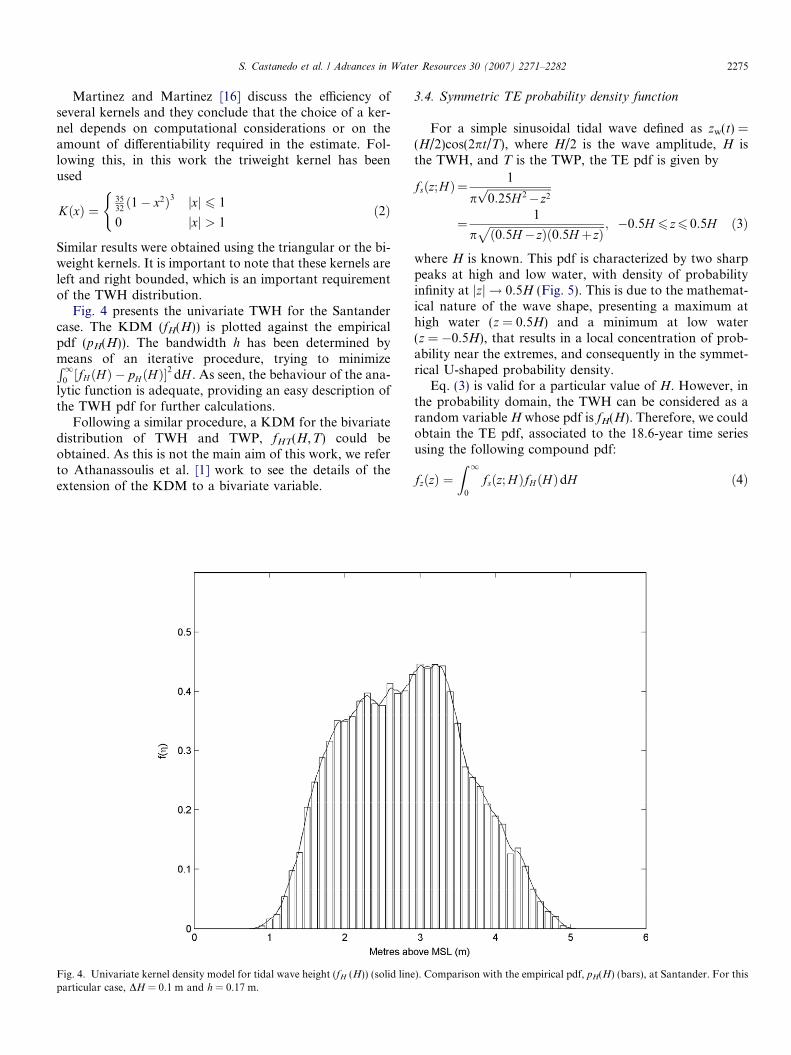
Fig. 4 presents the univariate TWH for the Santandercase. The KDM (fH(H)) is plotted against the empiricalpdf (pH(H)). The bandwidth h has been determined bymeans of an iterative procedure, trying to minimizeR1

0 ½fH ðHÞ � pH ðHÞ�2 dH . As seen, the behaviour of the ana-

lytic function is adequate, providing an easy description ofthe TWH pdf for further calculations.

Following a similar procedure, a KDM for the bivariatedistribution of TWH and TWP, fHT(H,T) could beobtained. As this is not the main aim of this work, we referto Athanassoulis et al. [1] work to see the details of theextension of the KDM to a bivariate variable.

Fig. 4. Univariate kernel density model for tidal wave height (fH (H)) (solid lineparticular case, DH = 0.1 m and h = 0.17 m.

3.4. Symmetric TE probability density function

For a simple sinusoidal tidal wave defined as zw(t) =(H/2)cos(2pt/T), where H/2 is the wave amplitude, H isthe TWH, and T is the TWP, the TE pdf is given by

fsðz;HÞ¼1

pffiffiffiffiffiffiffiffiffiffiffiffiffiffiffiffiffiffiffiffiffiffiffi0:25H 2� z2p

¼ 1

pffiffiffiffiffiffiffiffiffiffiffiffiffiffiffiffiffiffiffiffiffiffiffiffiffiffiffiffiffiffiffiffiffiffiffiffiffiffiffiffiffiffið0:5H � zÞð0:5H þ zÞ

p ; �0:5H 6 z6 0:5H ð3Þ

where H is known. This pdf is characterized by two sharppeaks at high and low water, with density of probabilityinfinity at jzj ! 0.5H (Fig. 5). This is due to the mathemat-ical nature of the wave shape, presenting a maximum athigh water (z = 0.5H) and a minimum at low water(z = �0.5H), that results in a local concentration of prob-ability near the extremes, and consequently in the symmet-rical U-shaped probability density.

Eq. (3) is valid for a particular value of H. However, inthe probability domain, the TWH can be considered as arandom variable H whose pdf is fH(H). Therefore, we couldobtain the TE pdf, associated to the 18.6-year time seriesusing the following compound pdf:

fzðzÞ ¼Z 1

0

fsðz; HÞfH ðHÞdH ð4Þ

). Comparison with the empirical pdf, pH(H) (bars), at Santander. For this

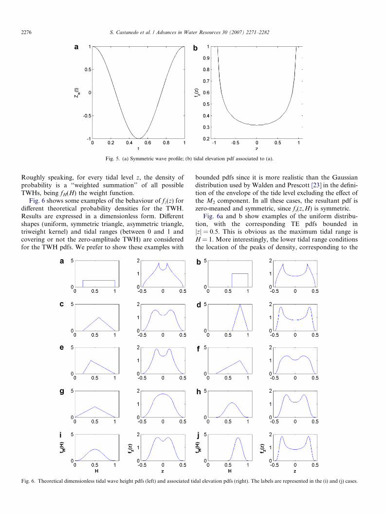
Fig. 5. (a) Symmetric wave profile; (b) tidal elevation pdf associated to (a).


Roughly speaking, for every tidal level z, the density ofprobability is a ‘‘weighted summation’’ of all possibleTWHs, being fH(H) the weight function.

Fig. 6 shows some examples of the behaviour of fz(z) fordifferent theoretical probability densities for the TWH.Results are expressed in a dimensionless form. Differentshapes (uniform, symmetric triangle, asymmetric triangle,triweight kernel) and tidal ranges (between 0 and 1 andcovering or not the zero-amplitude TWH) are consideredfor the TWH pdfs. We prefer to show these examples with

Fig. 6. Theoretical dimensionless tidal wave height pdfs (left) and associated ti

bounded pdfs since it is more realistic than the Gaussiandistribution used by Walden and Prescott [23] in the defini-tion of the envelope of the tide level excluding the effect ofthe M2 component. In all these cases, the resultant pdf iszero-meaned and symmetric, since fs(z,H) is symmetric.

Fig. 6a and b show examples of the uniform distribu-tion, with the corresponding TE pdfs bounded injzj = 0.5. This is obvious as the maximum tidal range isH = 1. More interestingly, the lower tidal range conditionsthe location of the peaks of density, corresponding to the

dal elevation pdfs (right). The labels are represented in the (i) and (j) cases.


minimum amplitudes of the TWH (jzj = 0.1 and jzj = 0.3for H = 0.2 and H = 0.6, respectively).

The slopes of the TE pdfs depend on the concentrationof probability of the TWH pdf. For example, Fig. 6f showsfor an asymmetrical triangular distribution of TWH (witha maximum of density of probability at H = 0.8), that themaximum slope is obtained in jzj = 0.4. Therefore, thehigher the density of probability in H, the higher the slopein the TE pdf in jzj = H/2. Logically, this result is due tothe U-shaped pdf for a particular sinusoidal wave that con-centrates a large amount of density of probability near thelower and upper bounds.

The location of the peaks of density is a combination ofthe different TWH, mainly governed by the neap tides, butit is not strictly defined by the lower TWH. These mostprobable levels are usually associated to a mean neap tide[19]. For the theoretical TWH pdfs presented in Fig. 6,the levels that correspond to the position of the peaksdepend on the shape of the TWH pdf. The two peaksdegenerate into just one peak in Fig. 6g, due to the zero-amplitude limit for the TWH. This unimodal pattern(example g) is usually associated to diurnal tides. In fact,the main factor responsible for this behaviour in diurnaltides is the similar amplitudes that usually present the O1

and K1 components, which form a 13.66-day group withnear zero-amplitude nodes.

Also note that the peaks are more pronounced (d and j)when the TWH pdf is narrower. Logically, the asymptoticcase would correspond to a Dirac Delta TWH pdf. For thiscase, we obtain Eq. (3) with both peaks having density ofprobability infinity.

Therefore, after this descriptive analysis covering differ-ent cases, one can deduce the shape of the TE pdf as a func-tion of the TWH pdf, as well as the TWH pdf as a functionof the TE pdf.

Note that in the aforementioned analysis, we haveavoided the dependence on the TWP. It is clear that theTE pdf depends also on the distribution of the periodsand we should consider a ‘‘weighted’’ summation depend-ing on the value of the period and using the joint distribu-tion of TWH and TWP, fHT(H,T), in the following way:

fzðzÞ ¼R1

0

R10

Tfsðz;HÞfHT ðH ; T ÞdH dTR10

R10

TfHT ðH ; T ÞdH dTð5Þ

Some tests were performed using Eq. (5) but the improve-ment was negligible, thus suggesting that making the model

Fig. 7. Horizontal axis: Tidal wave height, H (m). Vertical axis: crest (a) and tfunction of H. Data: Santander tidal gauge. Solid line: mean value of the par

more complicated is not worthwhile. Nevertheless, weshould be cautious with this fact if we wanted to use thisstatistical approach to analyze, for instance, tide-inducedmagnitudes such as the residual sediment transport [20,11].

3.5. Asymmetric TE probability density function

3.5.1. Parameterization of the asymmetry

The previous analysis shows that using the compoundpdf for symmetric waves may be a useful tool to estimatethe tide long-term water level distribution at a specific loca-tion. However, observing the examples shown in Fig. 1, itcan be seen that some of the TE pdfs exhibit an evidentasymmetry. The occurrence of tidal asymmetry is usuallyassociated to the generation of overtides (M4) in shallowwater areas [7]. Nevertheless, it has been recently demon-strated that the interaction (phase-locked patterns) of someastronomical tidal constituents, as for example K1 and O1

with M2, or M2 and S2 with MSf, may also cause tidalasymmetry (see i.e., [20,11,26]).

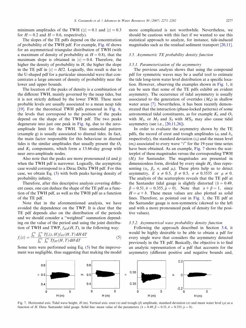
In order to evaluate the asymmetry shown by the TEpdfs, the record of crest and trough amplitudes (ai and bi,respectively), the standard deviation (si) and the mean level(mi) associated to every wave ‘‘i’’ for the 19-year time serieshave been obtained. As an example, Fig. 7 shows the scat-terplot of these magnitudes versus the corresponding TWH(Hi) for Santander. The magnitudes are presented indimensionless form, divided by every single Hi, thus repre-senting (ai, bi, ri and li). These plots help us to detectasymmetry, if a 5 0.5, b 5 0.5, r 5 0.3535 or l 5 0.The analysis of the scatterplots reveals that the TE pdf atthe Santander tidal gauge is slightly distorted ð�a ¼ 0:49;�b ¼ 0:51; �r ¼ 0:355; �l ¼ 0Þ. Note that a + b = 1, sinceH = a + b. These mean values are also plotted as solidlines. Therefore, as pointed out in Fig. 1, the TE pdf atthe Santander gauge is non-symmetric (skewed to the leftand with a more pronounced peak of density for the posi-tive values).

3.5.2. Asymmetrical wave probability density function

Following the approach described in Section 3.4, itwould be highly desirable to be able to obtain a pdf forevery single wave that considers the asymmetry detectedpreviously in the TE pdf. Basically, the objective is to findan analytic representation of a pdf that accounts for theasymmetry (different positive and negative bounds and,

rough (b) amplitude, standard deviation (r) and mean water level (l) as aameters ð�a ¼ 0:49; �b ¼ 0:51; �r ¼ 0:355; �l ¼ 0Þ.


consequently, different density of probability in the nega-tive and positive part of the function). Moreover, the pdfshould be expressed in terms of easily obtained parameters,such as the crest and trough amplitudes, and the standarddeviation of a single wave.

It has been found that the beta pdf is an adequateapproximate function to describe the above requirements[2]. This pdf is defined on the interval [�b + m,a + m]and can be expressed as

fBðz; a; b; s;mÞ ¼ ðzþ b� mÞq�1ða� zþ mÞr�1

ðaþ bÞqþr�1Bðq; rÞð6Þ

where q and r are parameters that must be greater thanzero and B is the beta function. The parameters q and r

are expressed as

q ¼ bðab� s2Þðaþ bÞs2

; r ¼ aðab� s2Þðaþ bÞs2

ð7Þ

Note that for a symmetric wave (a = b = 0.5H, s ¼ffiffiffi2p

H=4and m = 0), the parameters q = r = 0.5, and the beta pdfreduces to the one given in Eq. (3).

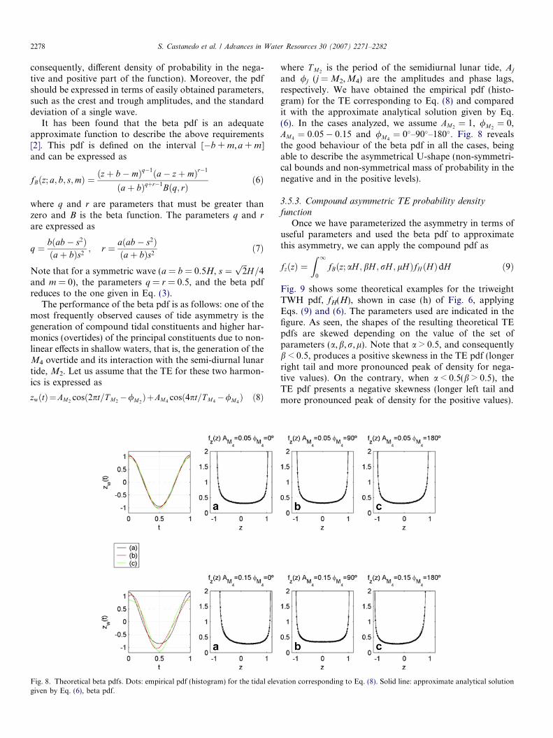
The performance of the beta pdf is as follows: one of themost frequently observed causes of tide asymmetry is thegeneration of compound tidal constituents and higher har-monics (overtides) of the principal constituents due to non-linear effects in shallow waters, that is, the generation of theM4 overtide and its interaction with the semi-diurnal lunartide, M2. Let us assume that the TE for these two harmon-ics is expressed as

zwðtÞ¼AM2cosð2pt=T M2

�/M2ÞþAM4

cosð4pt=T M4�/M4

Þ ð8Þ

Fig. 8. Theoretical beta pdfs. Dots: empirical pdf (histogram) for the tidal elevgiven by Eq. (6), beta pdf.

where T M2is the period of the semidiurnal lunar tide, Aj

and /j (j = M2,M4) are the amplitudes and phase lags,respectively. We have obtained the empirical pdf (histo-gram) for the TE corresponding to Eq. (8) and comparedit with the approximate analytical solution given by Eq.(6). In the cases analyzed, we assume AM2

¼ 1, /M2¼ 0,

AM4¼ 0:05� 0:15 and /M4

¼ 0�–90�–180�. Fig. 8 revealsthe good behaviour of the beta pdf in all the cases, beingable to describe the asymmetrical U-shape (non-symmetri-cal bounds and non-symmetrical mass of probability in thenegative and in the positive levels).

3.5.3. Compound asymmetric TE probability density

functionOnce we have parameterized the asymmetry in terms of

useful parameters and used the beta pdf to approximatethis asymmetry, we can apply the compound pdf as

fzðzÞ ¼Z 1

0

fBðz; aH ; bH ; rH ; lHÞfH ðHÞdH ð9Þ

Fig. 9 shows some theoretical examples for the triweightTWH pdf, fH(H), shown in case (h) of Fig. 6, applyingEqs. (9) and (6). The parameters used are indicated in thefigure. As seen, the shapes of the resulting theoretical TEpdfs are skewed depending on the value of the set ofparameters (a,b,r,l). Note that a > 0.5, and consequentlyb < 0.5, produces a positive skewness in the TE pdf (longerright tail and more pronounced peak of density for nega-tive values). On the contrary, when a < 0.5(b > 0.5), theTE pdf presents a negative skewness (longer left tail andmore pronounced peak of density for the positive values).

ation corresponding to Eq. (8). Solid line: approximate analytical solution

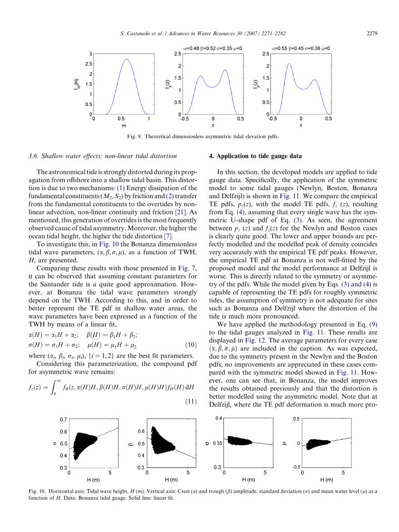
Fig. 9. Theoretical dimensionless asymmetric tidal elevation pdfs.


3.6. Shallow water effects: non-linear tidal distortion

The astronomical tide is strongly distorted during its prop-agation from offshore into a shallow tidal basin. This distor-tion is due to two mechanisms: (1) Energy dissipation of thefundamental constituents (M2,S2) by friction and (2) transferfrom the fundamental constituents to the overtides by non-linear advection, non-linear continuity and friction [21]. Asmentioned, this generation of overtides is the most frequentlyobserved cause of tidal asymmetry. Moreover, the higher theocean tidal height, the higher the tide distortion [7].

To investigate this, in Fig. 10 the Bonanza dimensionlesstidal wave parameters, (a,b,r,l), as a function of TWH,H, are presented.

Comparing these results with those presented in Fig. 7,it can be observed that assuming constant parameters forthe Santander tide is a quite good approximation. How-ever, at Bonanza the tidal wave parameters stronglydepend on the TWH. According to this, and in order tobetter represent the TE pdf in shallow water areas, thewave parameters have been expressed as a function of theTWH by means of a linear fit,

aðHÞ ¼ a1H þ a2; bðHÞ ¼ b1H þ b2;

rðHÞ ¼ r1H þ r2; lðHÞ ¼ l1H þ l2 ð10Þwhere (ai, bi, ri, li), {i = 1,2} are the best fit parameters.

Considering this parameterization, the compound pdffor asymmetric wave remains:

fzðzÞ ¼Z 1

0

fBðz; aðHÞH ; bðHÞH ; rðHÞH ; lðHÞHÞfH ðHÞdH

ð11Þ

Fig. 10. Horizontal axis: Tidal wave height, H (m). Vertical axis: Crest (a) andfunction of H. Data: Bonanza tidal gauge. Solid line: linear fit.

4. Application to tide gauge data

In this section, the developed models are applied to tidegauge data. Specifically, the application of the symmetricmodel to some tidal gauges (Newlyn, Boston, Bonanzaand Delfzijl) is shown in Fig. 11. We compare the empiricalTE pdfs, pz(z), with the model TE pdfs, fz (z), resultingfrom Eq. (4), assuming that every single wave has the sym-metric U-shape pdf of Eq. (3). As seen, the agreementbetween pz (z) and fz(z) for the Newlyn and Boston casesis clearly quite good. The lower and upper bounds are per-fectly modelled and the modelled peak of density coincidesvery accurately with the empirical TE pdf peaks. However,the empirical TE pdf at Bonanza is not well-fitted by theproposed model and the model performance at Delfzijl isworse. This is directly related to the symmetry or asymme-try of the pdfs. While the model given by Eqs. (3) and (4) iscapable of representing the TE pdfs for roughly symmetrictides, the assumption of symmetry is not adequate for sitessuch as Bonanza and Delfzijl where the distortion of thetide is much more pronounced.

We have applied the methodology presented in Eq. (9)to the tidal gauges analyzed in Fig. 11. These results aredisplayed in Fig. 12. The average parameters for every caseð�a; �b; �r; �lÞ are included in the caption. As was expected,due to the symmetry present in the Newlyn and the Bostonpdfs, no improvements are appreciated in these cases com-pared with the symmetric model showed in Fig. 11. How-ever, one can see that, in Bonanza, the model improvesthe results obtained previously and that the distortion isbetter modelled using the asymmetric model. Note that atDelfzijl, where the TE pdf deformation is much more pro-

trough (b) amplitude, standard deviation (r) and mean water level (l) as a

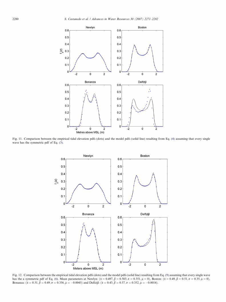
Fig. 12. Comparison between the empirical tidal elevation pdfs (dots) and the model pdfs (solid line) resulting from Eq. (9) assuming that every single wavehas the a symmetric pdf of Eq. (6). Mean parameters at Newlyn: ð�a ¼ 0:497; �b ¼ 0:503; �r ¼ 0:351; �l ¼ 0Þ, Boston: ð�a ¼ 0:49; �b ¼ 0:51; �r ¼ 0:35; �l ¼ 0Þ,Bonanza: ð�a ¼ 0:51; �b ¼ 0:49; �r ¼ 0:356; �l ¼ �0:0045Þ and Delfzijl: ð�a ¼ 0:43; �b ¼ 0:57; �r ¼ 0:352; �l ¼ �0:0014Þ.

Fig. 11. Comparison between the empirical tidal elevation pdfs (dots) and the model pdfs (solid line) resulting from Eq. (4) assuming that every singlewave has the symmetric pdf of Eq. (3).


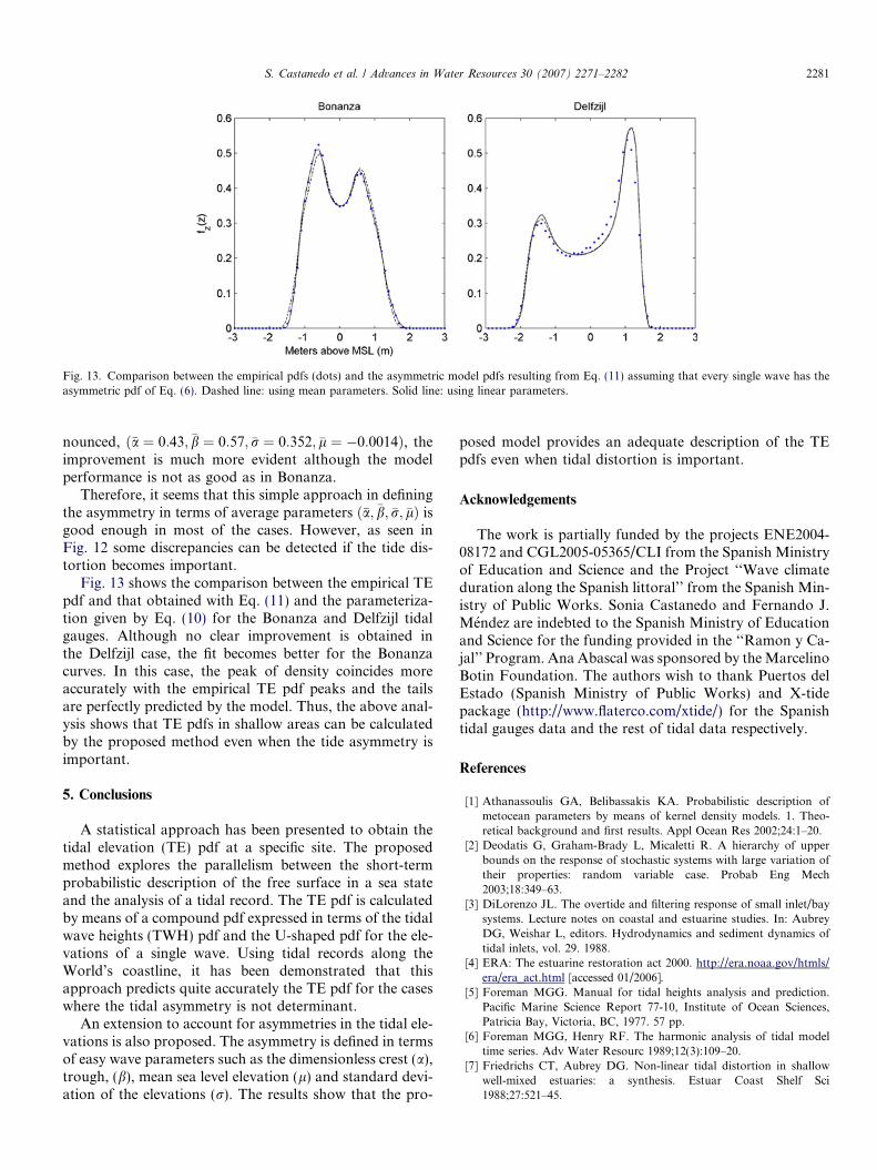
Fig. 13. Comparison between the empirical pdfs (dots) and the asymmetric model pdfs resulting from Eq. (11) assuming that every single wave has theasymmetric pdf of Eq. (6). Dashed line: using mean parameters. Solid line: using linear parameters.


nounced, ð�a ¼ 0:43; �b ¼ 0:57; �r ¼ 0:352; �l ¼ �0:0014Þ, theimprovement is much more evident although the modelperformance is not as good as in Bonanza.

Therefore, it seems that this simple approach in definingthe asymmetry in terms of average parameters ð�a; �b; �r; �lÞ isgood enough in most of the cases. However, as seen inFig. 12 some discrepancies can be detected if the tide dis-tortion becomes important.

Fig. 13 shows the comparison between the empirical TEpdf and that obtained with Eq. (11) and the parameteriza-tion given by Eq. (10) for the Bonanza and Delfzijl tidalgauges. Although no clear improvement is obtained inthe Delfzijl case, the fit becomes better for the Bonanzacurves. In this case, the peak of density coincides moreaccurately with the empirical TE pdf peaks and the tailsare perfectly predicted by the model. Thus, the above anal-ysis shows that TE pdfs in shallow areas can be calculatedby the proposed method even when the tide asymmetry isimportant.

5. Conclusions

A statistical approach has been presented to obtain thetidal elevation (TE) pdf at a specific site. The proposedmethod explores the parallelism between the short-termprobabilistic description of the free surface in a sea stateand the analysis of a tidal record. The TE pdf is calculatedby means of a compound pdf expressed in terms of the tidalwave heights (TWH) pdf and the U-shaped pdf for the ele-vations of a single wave. Using tidal records along theWorld’s coastline, it has been demonstrated that thisapproach predicts quite accurately the TE pdf for the caseswhere the tidal asymmetry is not determinant.

An extension to account for asymmetries in the tidal ele-vations is also proposed. The asymmetry is defined in termsof easy wave parameters such as the dimensionless crest (a),trough, (b), mean sea level elevation (l) and standard devi-ation of the elevations (r). The results show that the pro-

posed model provides an adequate description of the TEpdfs even when tidal distortion is important.

Acknowledgements

The work is partially funded by the projects ENE2004-08172 and CGL2005-05365/CLI from the Spanish Ministryof Education and Science and the Project ‘‘Wave climateduration along the Spanish littoral’’ from the Spanish Min-istry of Public Works. Sonia Castanedo and Fernando J.Mendez are indebted to the Spanish Ministry of Educationand Science for the funding provided in the ‘‘Ramon y Ca-jal’’ Program. Ana Abascal was sponsored by the MarcelinoBotin Foundation. The authors wish to thank Puertos delEstado (Spanish Ministry of Public Works) and X-tidepackage (http://www.flaterco.com/xtide/) for the Spanishtidal gauges data and the rest of tidal data respectively.

References

[1] Athanassoulis GA, Belibassakis KA. Probabilistic description ofmetocean parameters by means of kernel density models. 1. Theo-retical background and first results. Appl Ocean Res 2002;24:1–20.

[2] Deodatis G, Graham-Brady L, Micaletti R. A hierarchy of upperbounds on the response of stochastic systems with large variation oftheir properties: random variable case. Probab Eng Mech2003;18:349–63.

[3] DiLorenzo JL. The overtide and filtering response of small inlet/baysystems. Lecture notes on coastal and estuarine studies. In: AubreyDG, Weishar L, editors. Hydrodynamics and sediment dynamics oftidal inlets, vol. 29. 1988.

[4] ERA: The estuarine restoration act 2000. http://era.noaa.gov/htmls/era/era_act.html [accessed 01/2006].

[5] Foreman MGG. Manual for tidal heights analysis and prediction.Pacific Marine Science Report 77-10, Institute of Ocean Sciences,Patricia Bay, Victoria, BC, 1977. 57 pp.

[6] Foreman MGG, Henry RF. The harmonic analysis of tidal modeltime series. Adv Water Resourc 1989;12(3):109–20.

[7] Friedrichs CT, Aubrey DG. Non-linear tidal distortion in shallowwell-mixed estuaries: a synthesis. Estuar Coast Shelf Sci1988;27:521–45.


http://era.noaa.gov/htmls/era/era_act.html

http://era.noaa.gov/htmls/era/era_act.html


[8] Friedrichs CT, Aubrey DG. Tidal propagation in strongly convergentchannels. J Geophys Res 1994;99:3321–36.

[9] Goda Y. Random seas and design of maritime structures. In: LiuPhilip L-F, editor. Advanced series on ocean engineering, vol.15. Singapore: World Scientific; 2000.

[10] Godin G. The analysis of tides. Toronto: University of TorontoPress; 1972, ISBN 0802017479.

[11] Hoitink AJF, Hoekstra P, van Maren DS. Flow asymmetry associ-ated with astronomical tides: implications for the residual transportof sediment. J Geophys Res 2003;108(C10):3315. 13-1/13-8.

[12] Kreeke J, Iannuzzi RA. Second-order solution for damped cooscil-lating tide in narrow canal. J Hydraul Eng 1998;24:1253–60.

[13] Leggett, DJ, Cooper, N, Harvey, R. Coastal and estuarine managedrealignment-design issues. CIRIA; London. ISBN 0860176282. 2004.

[14] Li L, Barry DA, Stagnitti F, Parlange JY, Jeng DS. Beach water tablefluctuations due to spring-neap tides: moving boundary effects. AdvWater Resourc 2000;23:817–24.

[15] Li H, Jiao JJ. Influence of the tide on the mean watertable in anunconfined, anisotropic, inhomogeneous coastal aquifer. Adv WaterResourc 2003;26:9–16.

[16] Martinez WL, Martinez AR. Computational statistics handbook withMATLAB. Chapman & Hall/CRC; 2002.

[17] Niedowski, NL. New York State Salt Marsh Restoration andMonitoring Guidelines. http://www.dec.state.ny.us/website/dfwmr/marine/smguide.html>; 2000 [accessed 02/2006].

[18] Pawlowicz R, Beardsley B, Lentz S. Classical tidal harmonic analysisincluding error estimates in MATLAB using T_TIDE. ComputGeosci 2002;28:929–37.

[19] Pugh D. Changing sea levels. Effects of tides, weather andclimate. Cambridge University Press; 2004.

[20] Ranasinghe R, Pattiaratchi C. Tidal inlet velocity asymmetry indiurnal regimes. Cont Shelf Res 2000;20:2347–66.

[21] Speer PE, Aubrey DG. A study of non-linear tidal propagation inshallow inlet/estuarine systems. Part II. Theory. Estuar Coast ShelfSci 1985;21:207–24.

[22] Tiner RW. Wetland indicators: a guide to wetland identification,delineation, classification and mapping. CRC Press LLC; 1999,ISBN 0873718925.

[23] Walden AT, Prescott P. Statistical distributions for tidal elevations.Geophys J Roy Astronom Soc 1983;72:223–36.

[24] Walton TL. Setup and setdown in tidal bays and wetlands. EstuarCoast Shelf Sci 2002;55:789–94.

[25] WFD Directive 2000/60/EC of the European Parliament and of theCouncil establishing a framework for the Community action in thefield of water policy. <http://ec.europa.eu/environment/water/water-framework/index_en.html>; 2000 [accessed 02/2006].

[26] Woodworth PL, Blackman DL, Pugh DT, Vassie JM. On the role ofdiurnal tides in contributing to asymmetries in tidal probabilitydistribution functions in areas of predominantly semi-diurnal tide.Estuar Coast Shelf Sci 2005;64(2–3):235–40.

http://www.dec.state.ny.us/website/dfwmr/marine/smguide.html

http://www.dec.state.ny.us/website/dfwmr/marine/smguide.html

http://ec.europa.eu/environment/water/water-framework/index_en.html

http://ec.europa.eu/environment/water/water-framework/index_en.html

Long-term tidal level distribution using a wave-by-wave approach

Documents