Long term performance of buried high density ... - FDOT

FOREWORD

This study is a follow-up of the earlier Florida Department of Transportation-

funded project (P.I: Dr. D. V. Reddy) at Florida Atlantic University entitled

"Evaluation of Plastic Piping for Pipe for Pipe Culverts and Storm Sewers". It is a

new stand-along experimental and analytical investigation addressing the long-term

properties and life cycles with accelerated testing simulated by super-ambient

temperature levels. Considerable attention is focused in longitudinal bending of un

jointed and jointed pipe and environmental stress cracking of un-notched and notched

pipe rings in flexural creep. The investigation also contains a sizable amount of two-

dimensional and three dimensional finite element analysis of viscoelastic pipe-soil

interaction. The findings will enable the setting up of performance limits and the

development of practical guidelines for the selection, design, specification and

installation of HDPE piping for subsurface drainage of transportation facilities. The

performance indicators will be changes in design standards.

ACKNOWLEDGEMENTS

The Principal Investigator would like to thank the Florida Department of

Transportation (Contract # BB-466) for its generous financial support. Gratitude is

expressed to Mr. R. Powers, Assistant State Corrosion Engineer, and Mr. R. Kessler, State

Corrosion Engineer, Materials Division FDOT, Gainesville, FL, Contract Monitors, and

Mr. S. McLemore, State Drainage Engineer, Drainage Division FDOT, Tallahassee, for

their continuing interaction with invaluable input, encouragement, and guidance.

The administrative support of Dr. S.E. Dunn, Professor and Former Chairman,

Department of Ocean Engineering and Dr. J. T. Jurewicz, Dean of Engineering, Florida

Atlantic University, is gratefully acknowledged.

ABSTRACT

The primary goal of this study was to evaluate the service life of HDPE (High

density polyethylene) notched/unnotched joint pipes. The following experimental tasks

were carried out: i) procurement of materials, and fabrication of test setups; ii) creep

evaluation: The performance of buried pipes (notched/unnotched), subjected to live

loading, was studied in soil chambers for three levels of loading (service, 2/3 and 1/3 of

service). The long-term behavior was accelerated with super-ambient temperatures; iii)

field monitoring: Strains and diametral changes were measured for 10,000 hours. Type I

and Type II with/without notch ring specimens were tested in flexural creep for

environmental stress cracking. The analytical investigations of viscoelastic pipe-soil

interaction were as follows: i) extrapolation of the long-term performance at ambient

temperature, based on the Bi-directional and the Arrhenius methods and ii) 2-D Finite

Element Analysis with an approximate extension to 3-D performance evaluation, using the

software CANDE, iii) 3-D Finite Element Analysis.

The findings include: i) the deflection threshold (7.5% vertical change of diameter)

as the governing failure condition, ii) similar life predictions, for Bi-directional and

Arrhenius methods, with service lives of about 80 and 30 years at ambient temperature, for

unnotched and notched pipes, respectively, subjected to maximum loading, iii) reasonable

agreement between analytical (2-D and 3-D) and experimental values, and iv) reduced

creep modulus for the notched ring specimens.

Jointed pipe, embedded in soil with varying properties, was also investigated both

experimentally and analytically. The results show that longitudinal bending moment can

lead to leakage.

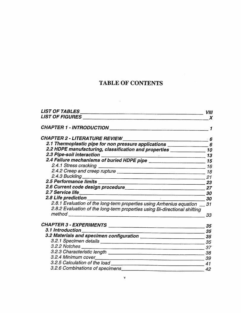
3.2.7 Installation of measuring devices……………………………………..44 3.2.7.1 Dial gages………………..………………..………………..………..44 3.2.7.2 Strain gages………………..………………..……………………….45

3.2.8 Soil chambers………………..………………..………………..………………..46 3.2.8.1 Schematic of the test setup………………..……………………….46 3.2.8.2 Design of the soil chambers………………..………………………46

3.2.9 Power supply………………..…………………..…………………..……………52 3.3 Performance of buried pipe, subjected to live load………………..…53

3.3.1 Fabrication and installation of soil chambers………………..……………….53 3.3.2 Filling the soil chambers with sand………………..…………………..………55 3.3.3 Application of the load………………..…………………..…………………..…56 CHAPTER 4 - RESULTS OF THE EXPERIMENTAL INVESTIGATION………..58

4.1 Sieve analysis…………………………………………………………………58 4.2 Soil compaction………………………………………………………………59 4.3 Test results of the performance of buried pipe, subjected to live loading………………………………………………………………………………63

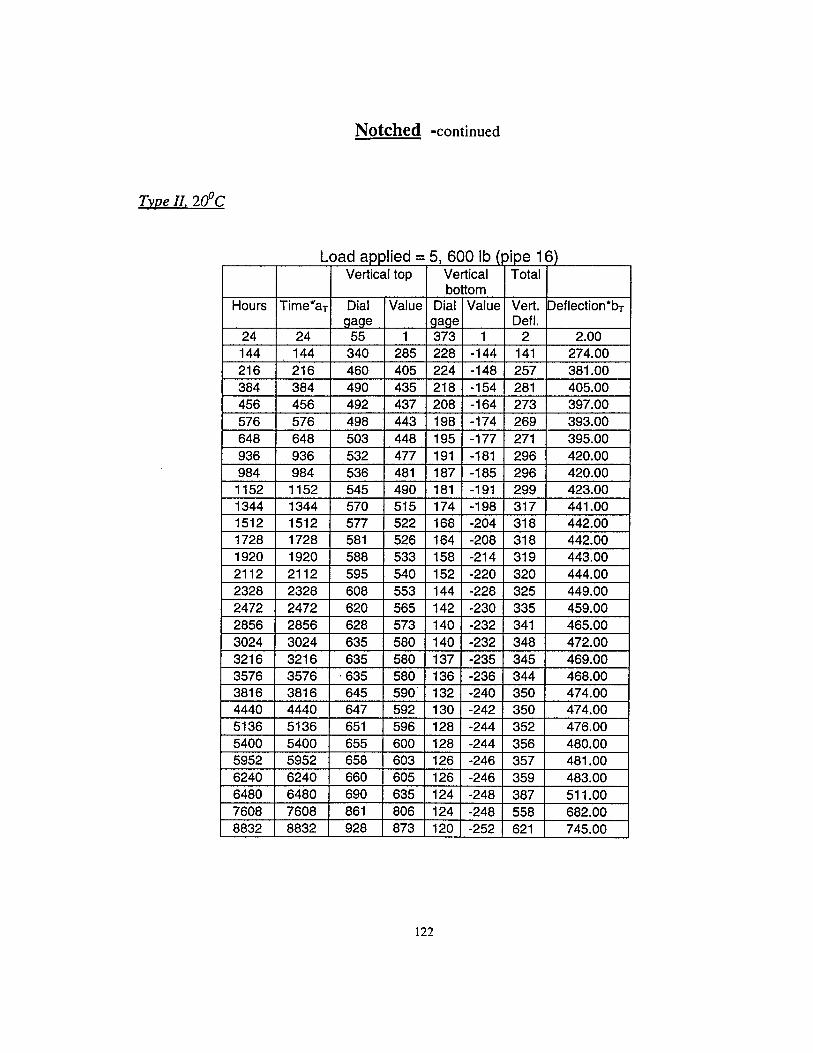
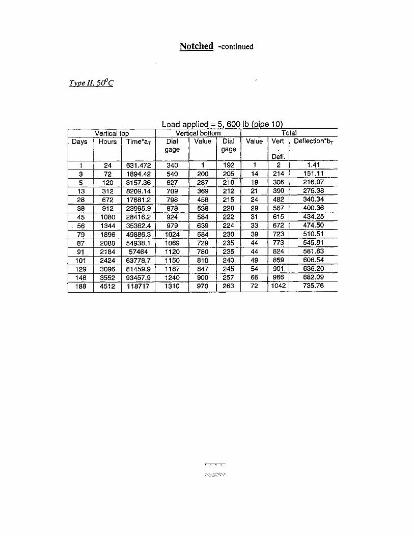
4.3.1 Vertical changes of diameter……………………………………………………63 Appendix A Deflection Data for Notched and Un-notched Pipes…………………64 4.3.2 Strains, stresses and moments…………………………………………………96

CHAPTER 5 -ANALYTICAL INVESTIGATION………………………………….102 5.1 Prediction of long-term properties…………………………………..…102 5.1.1 Evaluation of the long-term vertical change of diameter, using

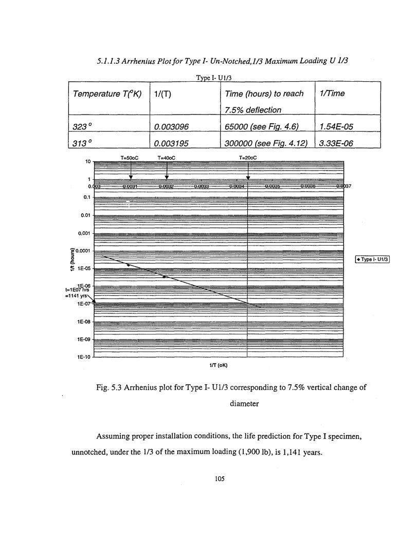
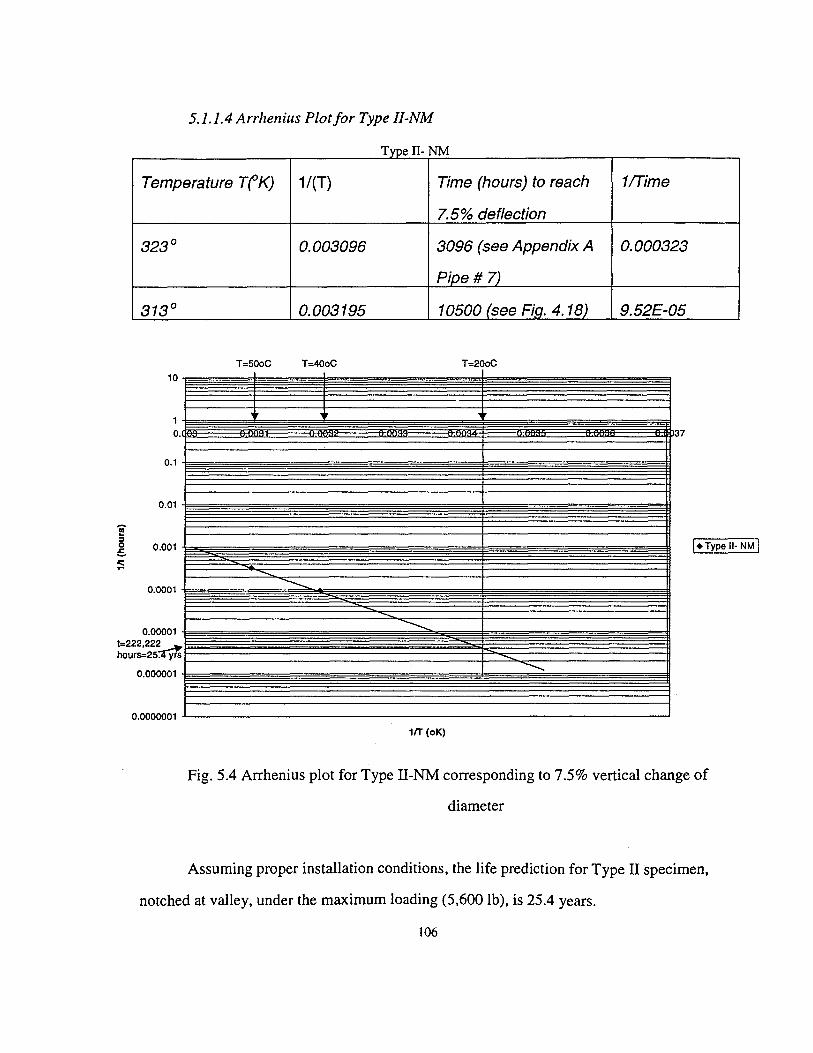
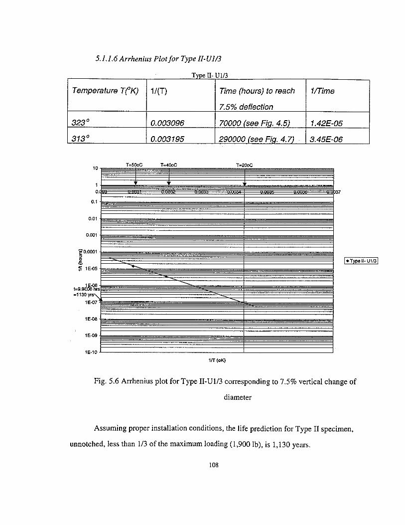
Arrhenius equation…………………………………………………………….102 5.1.1.1 Arrhenius plot for Type I-NM……………………………………...103 5.1.1.2 Arrhenius plot for Type I-UM……………………………………...104 5.1.1.3 Arrhenius plot for Type I-U1/3…………………………………….105 5.1.1.4 Arrhenius plot for Type II-NM……………………………………..106 5.1.1.5 Arrhenius plot for Type II-UM……………………………………..107 5.1.1.6 Arrhenius plot for Type II-U1/3…………………………………...108

5.1.2 Evaluation of the long-term vertical change of diameter, using Bi directional shifting method …………………………………………….……..109 Appendix B The values are for the Bi-directional method, which areshown

in Figs. 5.7 to 5.12…………………………………………………….…...110 5.1.2.1 Bi-directional plot for Type I-NM…………………………….……125 5.1.2.2 Bi-directional plot for Type I-UM………………………………….126 5.1.2.3 Bi-directional plot for Type I-U1/3………………………………..127 5.1.2.4 Bi-directional plot for Type II-NM…………………………………128 5.1.2.5 Bi-directional plot for Type II-UM…………………………………129 5.1.2.6 Bi-directional plot for Type II-U1/3……………………………….130

5.1.3 Comparison of Arrhenius and Bi-directional methods 131 5.2 CANDE analysis…………………………………………………………….131

5.2.1 General Information………………………….131 5.2.2 CANDE results 135 vi

CHAPTER 1

INTRODUCTION

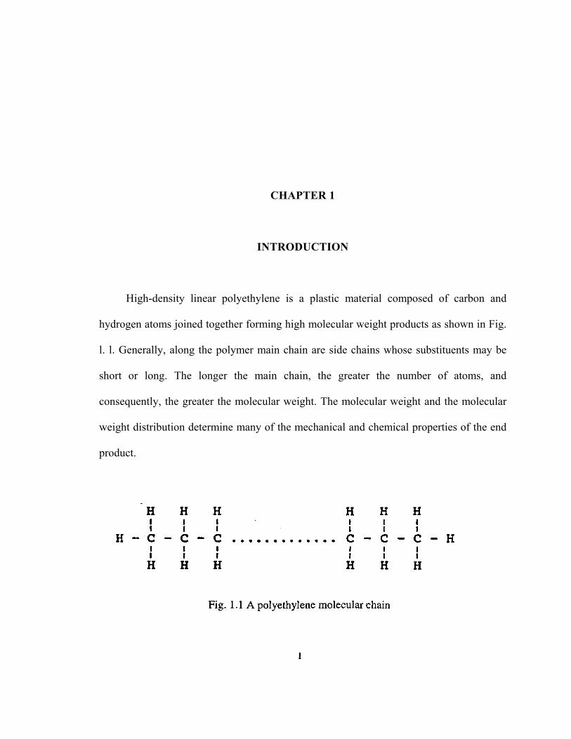
High-density linear polyethylene is a plastic material composed of carbon and

hydrogen atoms joined together forming high molecular weight products as shown in Fig.

l. l. Generally, along the polymer main chain are side chains whose substituents may be

short or long. The longer the main chain, the greater the number of atoms, and

consequently, the greater the molecular weight. The molecular weight and the molecular

weight distribution determine many of the mechanical and chemical properties of the end

product.

The arrangement of the molecular chains is predictive of the property

characteristics of polyethylene. Although shown flat and lying in a plane in Fig.l.l, the

molecular chains are three-dimensional and lie in wavy planes. Branching off the main

chains are side chains that may be of different lengths. The number, size, and type of

these side chains determine, in large part, the properties of density, stiffness, tensile

strength, flexibility, hardness, brittleness, elongation, creep characteristics, and melt

viscosity that distinguishes the manufacturing effort and service performance of

polyethylene pipe.

High-density polyethylene pipe (HDPE) has good potential for economic use for

marine oil and gas pipelines, under drains, storm sewers, culverts, and other subsurface

drainage structures. In view of its inherent chemical and corrosion resistance, lightweight,

toughness, flexibility, easy splicing, and consequent easy handling, and installation,

HDPE piping is being used extensively for gas pipelines. In the transportation industry,

over forty states use HDPE pipe as part of a 40% annual growth for the use of

thermoplastic, HDPE and polyvinyl chloride, (PVC) pipe in transportation construction

projects, [Goddard, 1995]. The long-term performance of HDPE is of particular interest,

in view of highly organic and salt-water (coastal) conditions.

Recently, based on field experience in California, concerns have been expressed,

[Johnson, 1993], [Strand, 1993], and [Hall and Foreman, 1993], about certain

inadequacies of high-density polyethylene piping. These include long-term strength and

stiffness (dimensional reliability) characteristics, delamination of the interior liner,

inconsistency of physical properties, buckling, opening of joints leading to infiltration

and exfiltration of water, tearing of corrugations and circumferential cracking of inner

liner, flammability, the requirement for excessive trench widths. But thirty state DOT

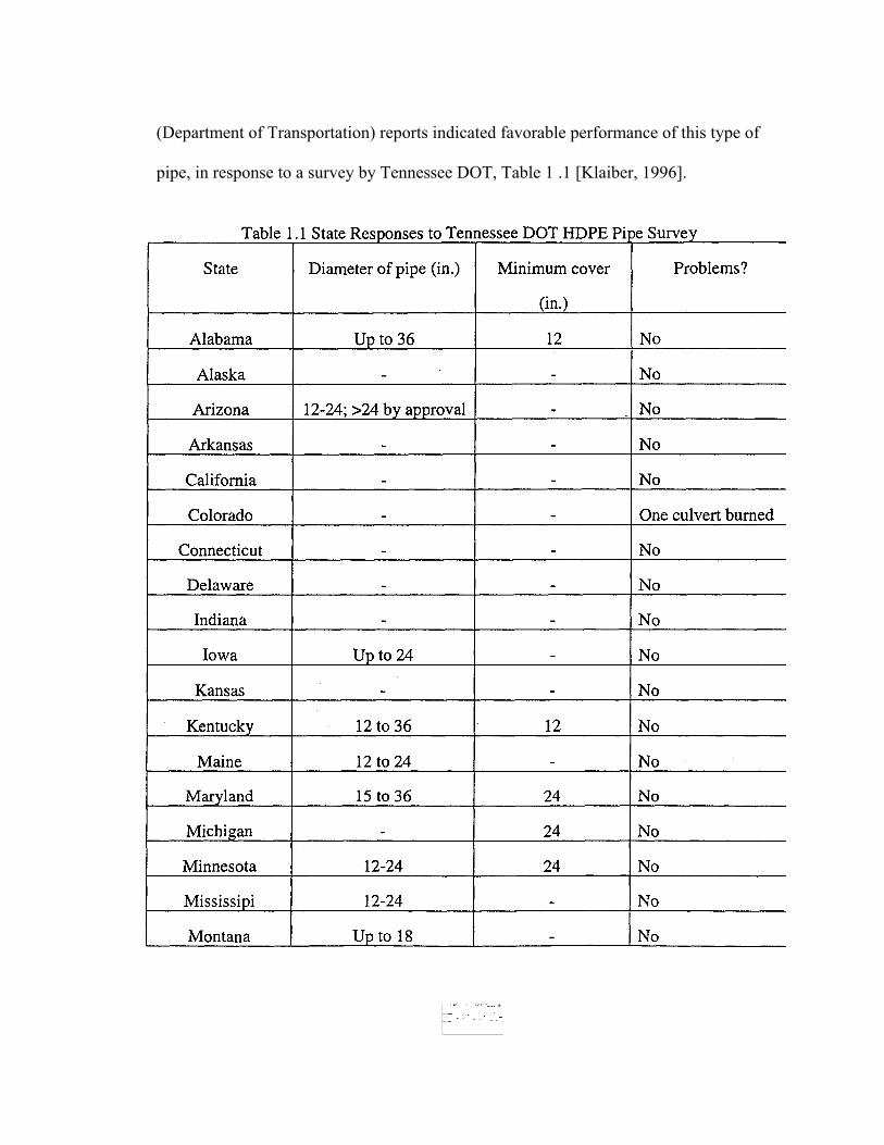
(Department of Transportation) reports indicated favorable performance of this type of

pipe, in response to a survey by Tennessee DOT, Table 1 .1 [Klaiber, 1996].

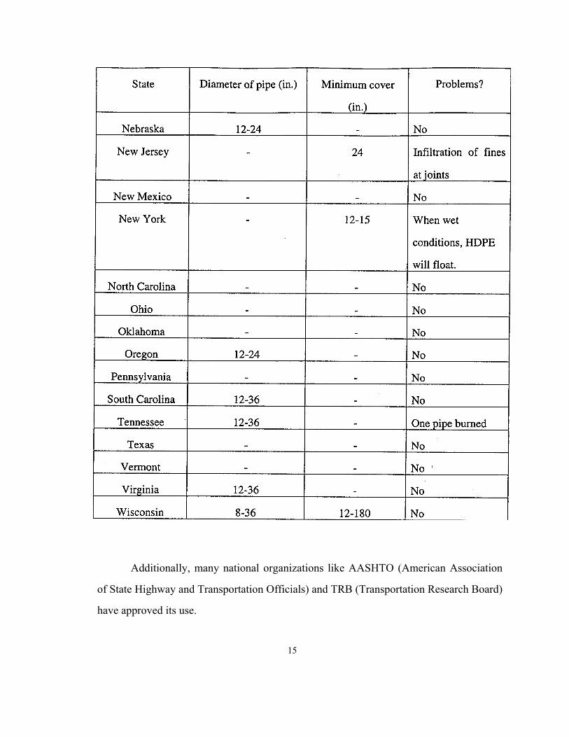
Additionally, many national organizations like AASHTO (American Association

of State Highway and Transportation Officials) and TRB (Transportation Research Board)

have approved its use.

15

The necessary considerations to ensure long-term performance of HDPE pipe

are as follows: 1) resin quality (strength and cracking), 2) profile stability (buckling

resistance), 3) adequate installation stiffness and backfill control, and 4) installed pipe

deflection levels. Items 1 and 2 are especially important in these long-term

applications due to the time dependent nature of the materials involved. Local

buckling can occur when sufficient compressive strain due to any combination of

deflection and ring compression occurs for each specific profile. Cracking occurs due

to localized tension stresses (strains) and stress concentration factors in the profile. For

long-term applications, both pipe deflection levels and the specific grade of the

material used must be controlled.

16

CHAPTER 2

LITERATURE REVIEW

2.1 Thermoplastic pipe for nonpressure applications

More than half of the entire thermoplastic pipe produced is used for nonpressure

applications. Most drainage systems, including those for building foundations, leaching

fields, agriculture, and road construction now consist of thermoplastic piping, mostly PE

and PVC. Both PE and PVC are increasingly used for larger-diameter sewers and culverts.

Thermoplastics, being nonconductors, are immune to the corrosion process induced by

electrolyte, such as acids and salts. In addition, plastic pipe materials are not vulnerable to

biological attack. This results in negligible costs for maintenance and external protection

such as painting, plastic coating, or cathodic protection. Their lower specific gravity

contributes to ease of handling, storage, and installation, as well as lower

6

transportation costs. They also offer very good abrasion resistance, even when conveying

slurries. High deformation capacity provides a positive pipe-soil interaction that is capable of

supporting earth fills and surface live loads of considerable magnitude without fracture.

Therefore, a sizable number of DOT (Department of Transportation) reports have indicated

favorable performance of this type of pipe, and many national organizations including

AASHTO (American Association of State Highway and Transportation Officials) approve its

use.

However, primarily based on some recent experiences in three field sites in

California, concerns have been expressed about the inadequacies of HDPE flexible piping,

and, by implication, about all thermoplastics for this application area; e.g. Johnson [1993),

Strand [1993], and Hall and Foreman [1993]. These concerns which must be resolved,

include long-term strength and stiffness (dimensional reliability) characteristics:

delamination of the interior liner, inconsistency of physical properties, buckling, opening of

joints leading to infiltration, and exfltration of water, tearing of corrugations and

circumferential cracking of the inner liner, flammability, and the requirement for excessive

trench widths. The development of data and methodologies for the safe and reliable use of

HDPE, PVC and other thermoplastics to allow them to be used in competition with other

pipe materials, is essential to assure cost-effective applications, which, in turn, would

enhance the utilization of public funds for highway construction and maintenance

operations.

To ensure long-term performance, the individual pipe wall profile must be evaluated

in regard to its specific geometry, and the stresses and strains quantified to properly

determine the long-term capacity of the specific materials allowed. Local buckling will occur

when sufficient compressive strain due to any combination of

7

deflection and ring compression occurs for each specific profile. Cracking occurs due to

localized tension stresses (strains) due to stress concentration factors and residual stresses in the

profile. For long-term applications, both pipe deflection levels and the specific grade of the

plastic used must be controlled. Specific items for control include the following:

1) Resin quality (strength and cracking)

2) 2) Profile stability (buckling resistance)

3) 3) Adequate installation stiffness and backfill control.

4) 4) Pipe deflection levels.

Items 1 and 2 are especially important in long-term applications.

The values of long-term performance limits depend very much on the design method.

The proof of any design theory should be how accurately it predicts the location, and the mode

of failure of the product under anticipated loading conditions. Unfortunately, current non-

pressure pipe design procedures do not pass this test, regardless of major pipe types [Goddard,

1994]. Performance limits that have been suggested for the design of buried gravity flow

thermoplastic pipes include: 1) deflection, 2) wall buckling, 3) wall strain, 4) wall crushing, 5)

longitudinal bending, 6) stress concentration, and 7) yielding.

A study of polyethylene pipe specifications carried out at California State University

by Gabriel, Bennett, and Schneier [1996], indicated that the HDB testing has only marginal

value in its ability to predict the long-term service performance of gravity flow non-pressure

pipes, and that its cost/benefit aspects are not persuasive. However, a

8

quantitative evaluation has not yet been made to set up performance limits and develop

practical guidelines for selection, design, specification, and installation.

Moser [1993, 1994] observed that "the normal and real modulus is the instantaneous

stress divided into the instantaneous short-term strain parameter for design and most

materials must be designed on a life basis". This was based on Hydrostatic Design Basis

(HDB) strength testing of the PVC pipe that had been in service for 15 years, in which the

modulus after unloading was the same as that when the pipe was manufactured. The

properties of HDPE pipe (viscoelastic material) are dependent on time, temperature, stress,

and rate of loading. Instantaneous testing cannot be expected to simulate material behavior

when subjected to stress or deformation for extended period of time. For life prediction,

consideration should be given to the estimation of long-term property values of the modulus

and strength under exposure conditions (pipe-soil interaction) that simulate the end-use

applications. The use of a pseudoviscoelastic modulus for the elastic modulus implies the

tacit use of a principle of viscoelasticity known as the "correspondence principle". This

principle states that the stresses in a viscoelastic body subjected only to constant applied

forces, will be exactly the same as they are in an elastic body subjected to the same set of

tractions [Christensen, 1971]. In contradistinction to constant internally pressurized pipe in

the gas industry, non-pressure pipe is subjected to mixed force and displacement boundary

20

2.2 HDPE manufacturing, classification and properties

Polyethylene is possibly the best-known member of the polyolefin family, derived from

polymerization of olefin gases. PE is a partly crystalline and partly amorphous material. The

properties of PE are determined by its molecular structure. PE consists of backbone of long

molecular chain from which short chain branches occasionally project. The length, type, and

frequency of distribution of these branches, as well as other parameters such as molecular

weight and distribution, determine the degree of crystallinity and network of molecules that

anchor the crystal-like regions to one another. These structural characteristics affect the short

and long-term mechanical properties. The extent of crystallinity of PE is reflected by density.

The higher density materials have more crystalline regions, which results in greater stiffness

and tensile strength.

To protect the polymer during processing, storage, and service, PE is blended with

small quantities of heat stabilizers, anti-oxidants, and ultra-violet (UV) screens or stabilizers.

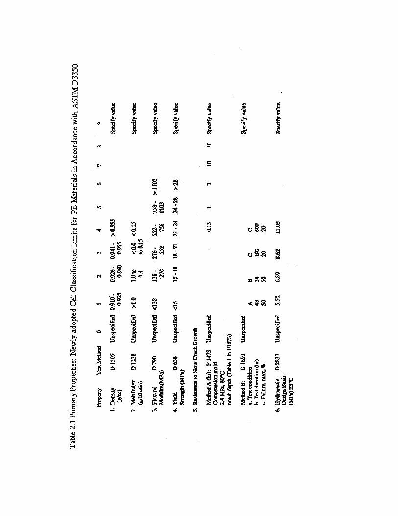
The primary specification for identifying and classifying PE piping materials is ASTM

D3350, entitled "Standard Specification for Polyethylene Pipe and Fitting Materials", Table

2.1. This specification identifies polyethylene pipe and fitting materials according to a cell

class format based on physical property criteria. The PE pipe compounds are classified

according to density, melt index, flexural modulus, tensile strength at yield, environmental

stress crack resistance, hydrostatic design basis at 23 oC (73.4 OF), color and UV stabilizers.

The order of these various properties is constant as shown in Table 2.1.

Due to the limitation of the current environmental stress crack resistance (ESCR) tests

(ASTM D 1693), an alternative test, the single point notched constant tensile load

10

(SP-NCTL) test (ASTM D 5397), was utilized in the study of Geosynthetic Research Institute

[Hsuan, 1999]. The cell classification should be modified to reflect changes in SCR tests. The

current cell class number for the ESCR is "T'. This number should be changed to "0", if the

SP-NCTL test is adopted. The specification should not require two different SCR tests. The

cell class "0" in ASTM d3350 is referred to "unspecified". Instruction for the SP-NCTL test

procedure and requirement should then be incorporated into the appropriate section (s) of the

specification to guide the user.

22

2.3 Pipe-soil interaction

Pipe-soil interaction addresses the mutual contributions of pipe and soil in a

successful structural system, as soil supports much of the vertical pressure in arching

action, over the pipe. The basic concept of the theory is that the load due to weight of the

soil column above the buried pipe is modified by arching action, in which a part of its

weight is transferred to the adjacent side prisms, with the result that in some cases the

load on the pipe may be less than the weight of the overlaying column of soil. Or, in the

other cases, the load on the pipe may be increased by an inverted.arch action, in which the

load from the side prisms is transferred to the soil over the pipe. The transferred force,

associated with arching action at the plane of the relative movement, is the resultant of

the vertical and horizontal components of force, Spangler [1982].

The "bedding" condition has a very important effect on both circumferential and

longitudinal bending moments. For instance, active lateral earth pressure can reduce the

circumferential moment by 25 %, Spangler [1982]. The longitudinal bending moments

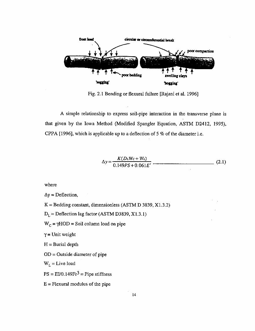
can also be affected similarly. Rajani et al. [1996] have indicated that flexural action due

to inadequate bedding support or swelling of underlying clay imposes longitudinal tensile

stresses, Fig. 2.1. Tensile stresses in the pipe can also be induced if clays with a high

montmorillonite mineral content undergo substantial volume change, when subjected to

seasonal wet and dry conditions. Clark [1971] and Morris [1967] have reported that

volumetric shrinkage for clays in Texas can be in the range of 14-40 percent.

24

I = Moment of inertia of the pipe wall F =

actual load applied

r = mean radius

E'= Backfill modulus

This clearly indicates that the deflection of a soil-embedded pipe depends on the

relative stiffness of the pipe and soil. There is a likelihood of long-term decomposition in

organic soil, which can reduce the arching action. Also, the physico-chemical stability of

certain limestone gravel can be detrimentally affected by dissolution due to groundwater

changes. The change in the degree of compaction near the pipe, and the consequent change in

K, can occur during installation, and/or service due to soil saturation or pumping. This can

also cause separation of the pipe wall from the soil. Therefore, it is important to address the

possible decrease of the arching effect in the life prediction of HDPE pipe. The same type of

soil changes can induce significant longitudinal stresses due to differential settlement-induced

beam action with non-uniform subgrade modulus.

2.4 Failure mechanisms of buried HDPE pipe

The major failure modes for thermoplastic pipes include buckling, and ductile/brittle

failures. Slow crack growth or rapid crack propagation characterizes some of these. For

pressurized pipes, ductile and brittle failures are of the utmost importance, as buckling is

seldom a major concern. In contrast, buckling is the most common failure mechanism in non-

pressure applications, with the remaining two failure modes being possible only in highly

unusual conditions. Note that in this discussion "brittle" is one that is produced in a long time

period under relatively low stress, is accompanied by little or no ductility, and is initiated at an

intrinsic weakness, (i.e. impurities, notches) in the

15

material. Slow crack growth (SCG), which is actually the same process, will here be used to

describe failures that initiate from larger artificial defects introduced in installation or service.

2.4.1 Stress cracking

Stress cracking is a macro-brittle cracking phenomenon that occurs at a constant stress

significantly less than the yield or break stress of the material. It is initiated at an internal or

external "defect" in the material such as an inclusion or scratch. In HDPE components, although

the stress crack is not associated with any apparent adjacent material deformation, the fracture

face itself provides evidence of ductility on a microscopic scale. In most cases, failure occurs as a

result of some unknown material performance characteristic, or some unexpected local service

condition that initiates a crack at a "flaw" in the material. It is necessary to identify such

unexpected failure initiating defects, and to understand at what rate induced cracks will propagate,

and how much they reduce the service life [Reddy, 1996].

The predominant mode of premature failure of thermoplastic pipe is a quasibrittle

fracture initiated at stress concentrating surface notch geometry and/or unexpected point stress,

Peggs and Kanninen [1995]. Such failures occur due to the fundamental stress cracking

susceptibility. The stress cracking is often called "Slow Crack Growth (SCG)", which occurs at

stress levels lower than the tensile yield strength, and at any time during the life of a pipe.

The material does not become brittle; it simply shows the appearance of brittleness. Stress

cracking is a synergistic function of applied stress, temperature, and

16

many material parameters (e.g. molecular weight and its distribution, commoner type and

content, and crystallinity). Stress cracking is most commonly thought to occur when the tie

molecules, which links crystalline and amorphous regions, slowly slip out from the region of

crystallinity involving entangled loose ends of tie molecules [Lustiger, 1983]. Fracture thus

occurs between crystalline regions involving amorphous polymer only, without apparent

deformation, and with relatively smooth fracture face morphology in HDPE. In contrast, when

HDPE is subjected to rapid increase in stress, as in a typical uniaxial tensile test, the tie

molecules do not have time to slip out of their entanglement, but instead, pull segments of the

crystalline region with them, producing the necking and elongation associated with yielding.

In the design of HDPE for storm-water sewer applications, a number of performance

limits need to be considered. In addition to well-established limit states, such as buckling and

excessive deflection, the maximum circumferential bending stresses in the pipe have to be

considered to avoid tensile yield or rupture of the pipe. Recently, it has also been suggested

that buried plastic pipe may be susceptible to slow crack growth following environmental

stress cracking or some other crack initiation mechanism. It has been established that slow

crack growth will only occur in a tensile stress field, Kuhlman, Weed, and Campbell [1995].

Furthermore, index tests developed for the gas pressure pipeline industry, reveal that the speed

at which slow crack growth occurs is affected by the magnitude of that maximum tensile

stress. Materials exhibiting low ductility can fail prematurely in a crack-like fashion (brittle

fracture) by slow crack growth.

The potential for stress cracking of plastic pipe is not a function of material properties

alone, as geometry plays an important role, Gabriel, Bennett, and Schneir [1996]. The NCTL

(Notch Constant Tensile Load), ASTM D5397, does not address the

17

relationship between stiffness and stress crack initiation with the focus on geometry. It is

necessary to identify unexpected failure-initiated defects and to understand their rate of

propagation, and the associated possible effects on excessive deflection and buckling. Stress

cracking failure in pipe, which is well presented in the Gas Research Institute's Field Failure

Catalog for Polyethylene Gas Piping, occurs predominantly at notch geometry associated

with joints. It also happens at locations where rocks impinge against the pipe surface, and at

locations that have been improperly squeezed off while making repairs, Peggs and Kanninen

[1995]. The stress-cracking problem in pipe was identified in the late 1970's. It was subject of

much research in the early. 1980's, resulting in significant improvements in stress cracking

resistance of pipe grade resins.

2.4.2 Creep and creep rupture

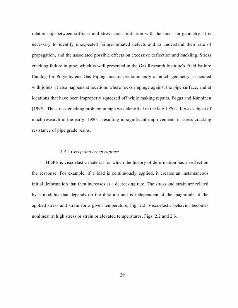
HDPE is viscoelastic material for which the history of deformation has an effect on

the response. For example, if a load is continuously applied, it creates an instantaneous

initial deformation that then increases at a decreasing rate. The stress and strain are related

by a modulus that depends on the duration and is independent of the magnitude of the

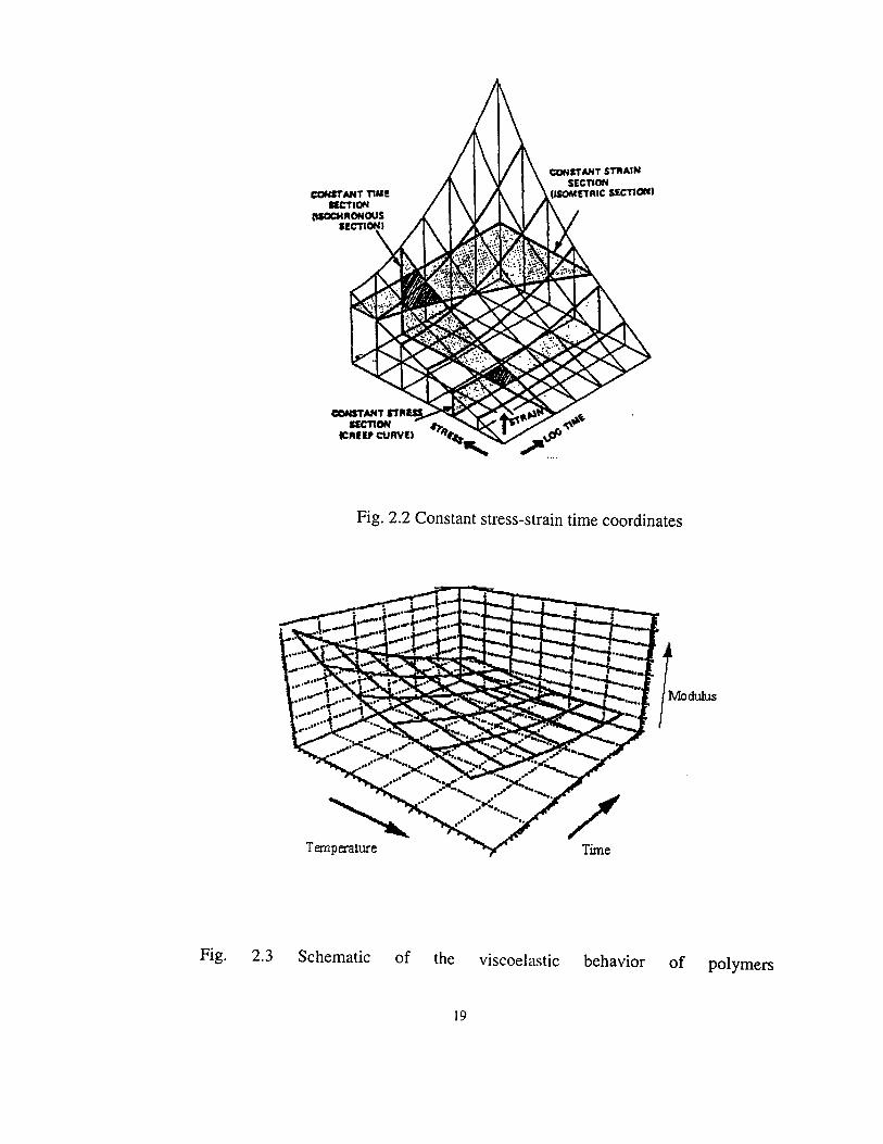
applied stress and strain for a given temperature, Fig. 2.2. Viscoelastic behavior becomes

nonlinear at high stress or strain or elevated temperatures, Figs. 2.2 and 2.3.

29

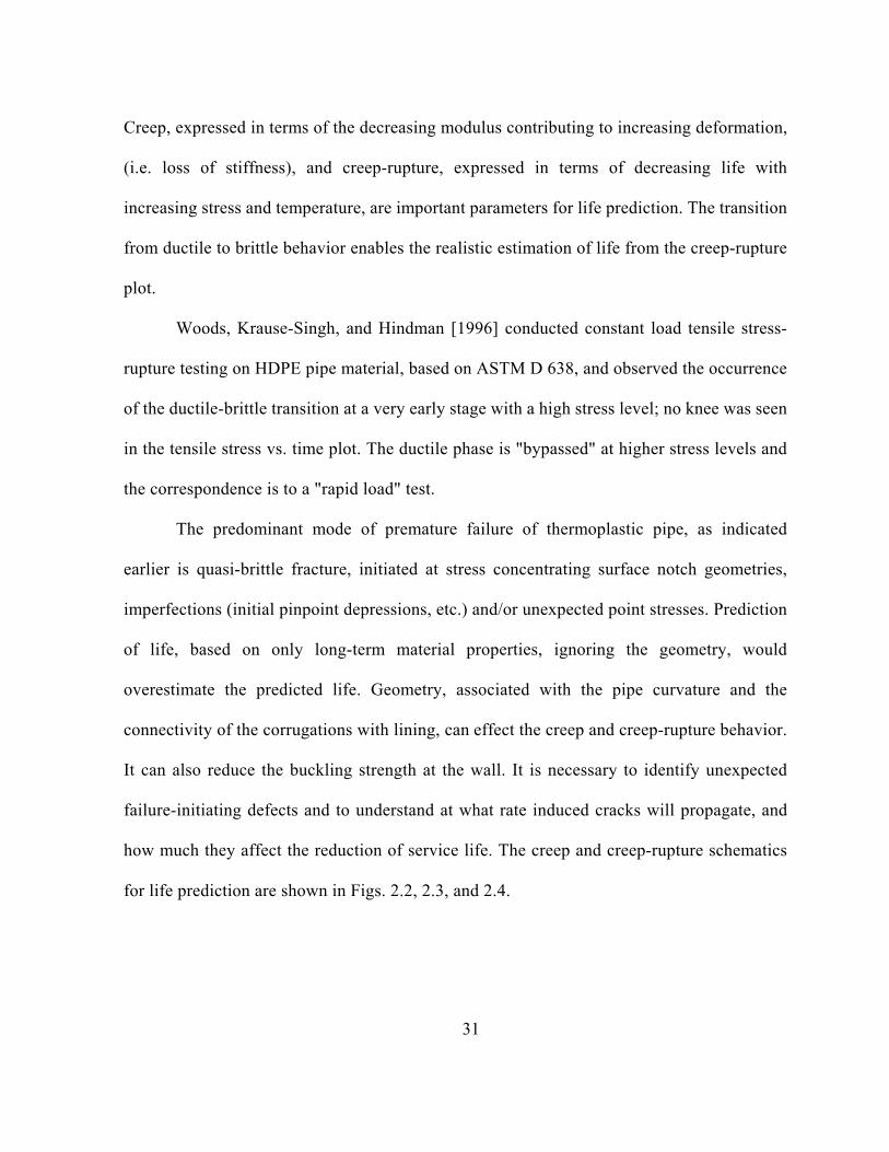
Creep, expressed in terms of the decreasing modulus contributing to increasing deformation,

(i.e. loss of stiffness), and creep-rupture, expressed in terms of decreasing life with

increasing stress and temperature, are important parameters for life prediction. The transition

from ductile to brittle behavior enables the realistic estimation of life from the creep-rupture

plot.

Woods, Krause-Singh, and Hindman [1996] conducted constant load tensile stress-

rupture testing on HDPE pipe material, based on ASTM D 638, and observed the occurrence

of the ductile-brittle transition at a very early stage with a high stress level; no knee was seen

in the tensile stress vs. time plot. The ductile phase is "bypassed" at higher stress levels and

the correspondence is to a "rapid load" test.

The predominant mode of premature failure of thermoplastic pipe, as indicated

earlier is quasi-brittle fracture, initiated at stress concentrating surface notch geometries,

imperfections (initial pinpoint depressions, etc.) and/or unexpected point stresses. Prediction

of life, based on only long-term material properties, ignoring the geometry, would

overestimate the predicted life. Geometry, associated with the pipe curvature and the

connectivity of the corrugations with lining, can effect the creep and creep-rupture behavior.

It can also reduce the buckling strength at the wall. It is necessary to identify unexpected

failure-initiating defects and to understand at what rate induced cracks will propagate, and

how much they affect the reduction of service life. The creep and creep-rupture schematics

for life prediction are shown in Figs. 2.2, 2.3, and 2.4.

31

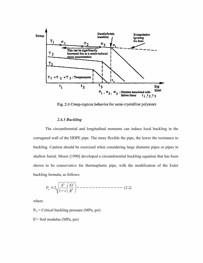
2.4.3 Buckling

The circumferential and longitudinal moments can induce local buckling in the

corrugated wall of the HDPE pipe. The more flexible the pipe, the lower the resistance to

buckling. Caution should be exercised when considering large diameter pipes or pipes in

shallow burial. Moser [1990] developed a circumferential buckling equation that has been

shown to be conservative for thermoplastic pipe, with the modification of the Euler

buckling formula, as follows:

−−−−−−−−−−−−−−−

−= 31

'2REI

vEPcr (2.2)

where

Pcr = Critical buckling pressure (MPa, psi)

E'= Soil modulus (MPa, psi)

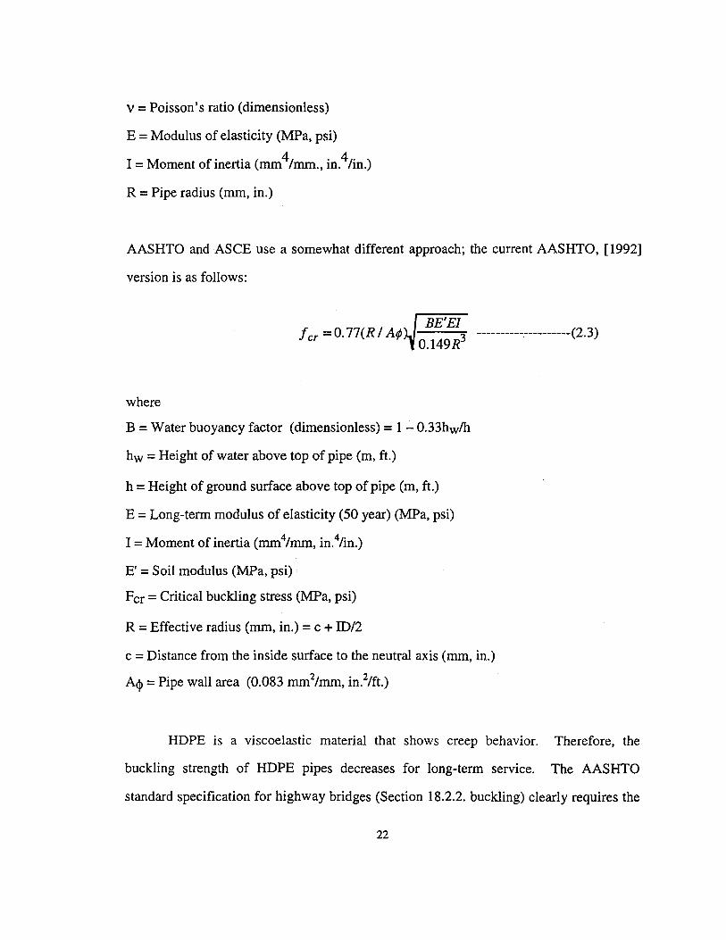
use of the 50-year modulus of elasticity for conservative buckling analysis, instead of the initial

modulus of elasticity.

Based on the hoop compression tests carried out by Selig, DiFrancisco, and McGrath

[1993], Moore and Laidlaw [1997] evaluated local buckling in the sidewall of the corrugation,

the valley and the crown. Local sidewall buckling was characterized by the development of

waviness in the element or sidewall. The phenomenon typically commenced atone location,

spread, and became more pronounced at higher hoop strains, thus involving most of the pipe

circumference. Valley buckling typically featured a lateral torsional response. This was

generally at a location, where the sidewall buckling was also present, with possible significant

interaction between the two elements of the profile. In his field inspection of pipe, buried under

Route I-279 north of Pittsburgh, PA, Selig [1990-1993], observed buckling of the unsupported

parts of the liner (between corrugation crests). These buckles were located in the bottom half of

the pipe [Selig, 1995]. This is a natural consequence of the ring compression of the wall.

Inaddition, circumferential cracking of inside crests was also observed in the corrugated

sections with the area covered by the coupling. He mentioned that this was probably a

longitudinal stress problem associated with coupling.

For a pipe tested under hoop compression, [Selig et al. 1993] carried out a numerical

prediction of critical hoop strain using a stiffened plate model and expressed buckling in terms

of critical hoop strain. Local soil support was found to have an important effect on the edge

restraint that influences the buckling strength, Moore and Laidlaw [1997). It was assumed that

the pipe was subjected to a uniform component of radial stress acting around the pipe

circumference, due to arching. However, when the arching action is affected by degradation in

soil properties, the vertical pressure in the

23

soil above the pipe is greater than the lateral pressure, and an ovaling deformation

results. Interactive longitudinal and circumferential bending can cause the local wall

buckling due to changes in bedding uniformity over a long-term, possible poor

installation, or ground saturation. Therefore, it is necessary to investigate the buckling

strength under combined circumferential and longitudinal bending. The time-dependent

buckling strength needs to be correlated with creep and creep-rupture; the effect of

possible damage should be considered for the long-term performance of HDPE pipe.

2.5 Performance limits

Prior to developing a design procedure, performance limits must be established.

The performance limits of buried HDPE pipe are related to stress, strain, deflection, or

buckling. The values of these limits depend on the design method used. The following is

a list of performance limits that are suggested in the literature for the design of buried,

HDPE pipe and culverts [Goddard, 1994].

i) Deflection: This limit is quite important due to relatively low bending stiffness

compared to concrete or metal pipes. Also, the stiffness decreases with time during the

service period. Excessive deformation can limit the flow or joint leakage. The limits are

set to avoid pipe-flattening, reversal of curvature, limit bending stresses, or bending

strains. However, deflection of pipes that are flexible in bending is controlled mainly by

the method of installation and in-situ soil envelope nronerties. Fig. 2.5.

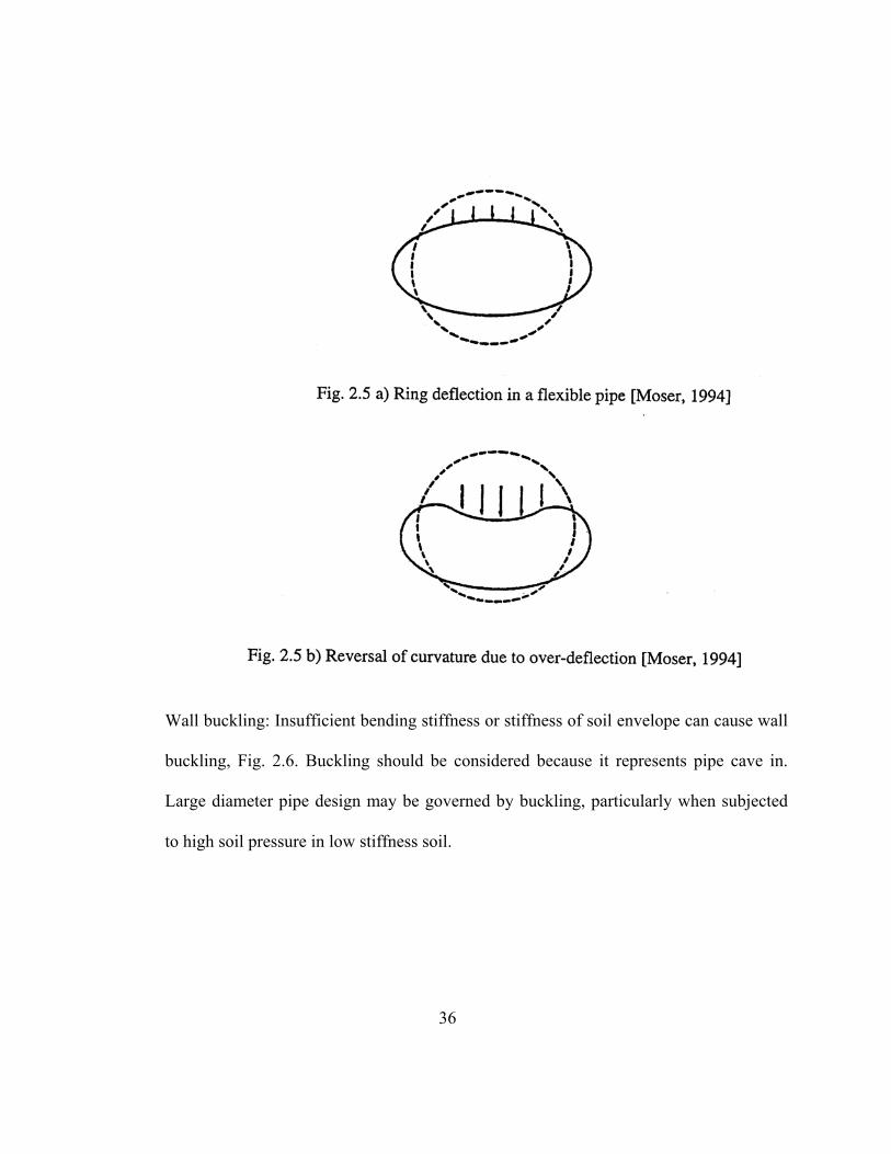
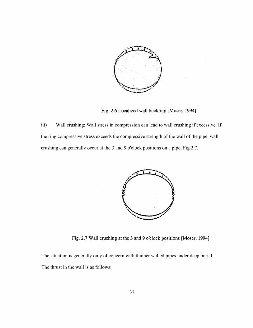
Wall buckling: Insufficient bending stiffness or stiffness of soil envelope can cause wall

buckling, Fig. 2.6. Buckling should be considered because it represents pipe cave in.

Large diameter pipe design may be governed by buckling, particularly when subjected

to high soil pressure in low stiffness soil.

36

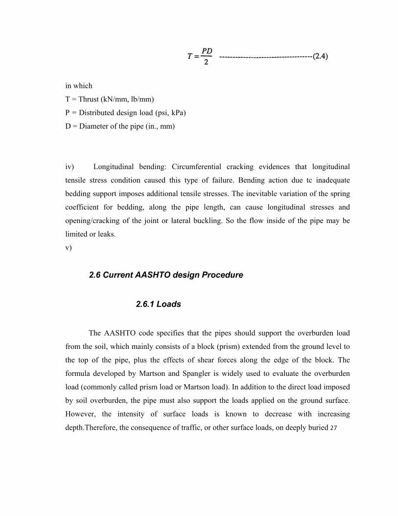
iii) Wall crushing: Wall stress in compression can lead to wall crushing if excessive. If

the ring compressive stress exceeds the compressive strength of the wall of the pipe, wall

crushing can generally occur at the 3 and 9 o'clock positions on a pipe, Fig 2.7.

The situation is generally only of concern with thinner walled pipes under deep burial.

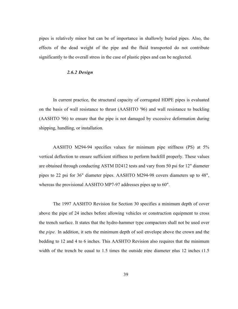
The thrust in the wall is as follows:

37

in which

T = Thrust (kN/mm, lb/mm)

P = Distributed design load (psi, kPa)

D = Diameter of the pipe (in., mm)

iv) Longitudinal bending: Circumferential cracking evidences that longitudinal

tensile stress condition caused this type of failure. Bending action due tc inadequate

bedding support imposes additional tensile stresses. The inevitable variation of the spring

coefficient for bedding, along the pipe length, can cause longitudinal stresses and

opening/cracking of the joint or lateral buckling. So the flow inside of the pipe may be

limited or leaks.

v)

2.6 Current AASHTO design Procedure

2.6.1 Loads

The AASHTO code specifies that the pipes should support the overburden load

from the soil, which mainly consists of a block (prism) extended from the ground level to

the top of the pipe, plus the effects of shear forces along the edge of the block. The

formula developed by Martson and Spangler is widely used to evaluate the overburden

load (commonly called prism load or Martson load). In addition to the direct load imposed

by soil overburden, the pipe must also support the loads applied on the ground surface.

However, the intensity of surface loads is known to decrease with increasing

depth.Therefore, the consequence of traffic, or other surface loads, on deeply buried 27

pipes is relatively minor but can be of importance in shallowly buried pipes. Also, the

effects of the dead weight of the pipe and the fluid transported do not contribute

significantly to the overall stress in the case of plastic pipes and can be neglected.

2.6.2 Design

In current practice, the structural capacity of corrugated HDPE pipes is evaluated

on the basis of wall resistance to thrust (AASHTO '96) and wall resistance to buckling

(AASHTO '96) to ensure that the pipe is not damaged by excessive deformation during

shipping, handling, or installation.

AASHTO M294-94 specifies values for minimum pipe stiffness (PS) at 5%

vertical deflection to ensure sufficient stiffness to perform backfill properly. These values

are obtained through conducting ASTM D2412 tests and vary from 50 psi for 12" diameter

pipes to 22 psi for 36" diameter pipes. AASHTO M294-98 covers diameters up to 48",

whereas the provisional AASHTO MP7-97 addresses pipes up to 60".

The 1997 AASHTO Revision for Section 30 specifies a minimum depth of cover

above the pipe of 24 inches before allowing vehicles or construction equipment to cross

the trench surface. It states that the hydro-hammer type compactors shall not be used over

the pipe. In addition, it sets the minimum depth of soil envelope above the crown and the

bedding to 12 and 4 to 6 inches. This AASHTO Revision also requires that the minimum

width of the trench be equal to 1.5 times the outside pipe diameter plus 12 inches (1.5

39

2.6.3 Pipe resistance and stiffness

Structural strength and rigidity against external loads for HDPE pipes are

established by load tests performed according to ASTM D2412. In the load test, equal and

opposite concentrated loads are applied on opposite ends of the diameter. The pipe

stiffness and related buckling resistance are determined from the load deflection data.

2.6.3 Design life

The service lives of corrugated HDPE pipes are dependent upon many factors such

as load magnitude, duration and history, temperature, and moisture, as well as longterm

durability performance with regards to aggressive environments. Under adverse loading

and environmental conditions, corrugated HDPE pipes subjected to the action of a

constant load may fail after a certain period, referred to as the endurance line. This

phenomenon, known as creep rupture, exists for all structural materials. As the ratio of the

sustained stress to the short-term strength increases, the endurance time (i.e. time to

rupture) decreases.

The design procedure specified by AASHTO Standards recognizes the time

dependence of the stress-strain relationship by allowing the use of long-term (e.g. 50year-

service life expectancy) tensile strength regression value. Also, the AASHTO code

requires the use of 50-year modulus of elasticity when designing for buckling

(AASHTO'96) and sets the allowable long-term strain to 5%.

2.7 Service life

The current AASHTO code requirements and practice are adequate for a

conservative design of corrugated HDPE pipes buried at 17 feet or less, provided that

[FDOT, 1999]:

(a) the backfill soil has a minimum stiffness E'=2,000 psi and a 95% minimum

compaction; (b) only HDPE pipes with annular corrugations are allowed; (c) the

minimum width of the trench is equal to 1.5 times the outside pipe diameter (O.D.) plus

12 in. (1.5 O.D. + 12 in.); (d) the minimum cover above the crown of the pipe is 24

inches before allowing vehicles or construction equipment to cross the trench; (e) the

irregularities of the bedding surface (grade control) are limited to 1 % of a single section

of pipe; (f) the so-called bell-and-spigot extruded joints, such as ADS Pro-Link Ultra or

Hancor Hi-Q Sure-Lok, meeting the AASHTO requirements are used.

2.8 Life prediction

There is an identified need to investigate the long-term behavior in relatively short

laboratory time scale, by evaluating the effect of soil degradation mechanisms at field-

related temperatures and stresses, compounded by synergistic effects, with accelerated

testing, high stress, elevated temperatures, and/or aggressive liquids.

It is noteworthy that the type of material qualification testing, used for natural gas

distribution piping, has very effectively screened out one failure mode: ductile failure.

dependence of polyethylene and other thermoplastic materials, it is both possible and necessary to

accelerate the failure mechanism. The key is the use of time-temperature shifting functions that

can reliably connect high temperature/high pressure performance to actual service conditions.

The long-term properties can be predicted based on viscoelastic behavior: i) the Arrhenius

equation [Koerner, 1994], which describes the temperature dependency of the degradation

reaction on time and temperature, ii) the Bi-directional method, which determines the curve that

fits the time-to-failure test data at elevated temperatures to enable predictions of times-to-failure

at lower temperatures, [Popelar, 1993]

2.8.1. Evaluation of the long-term properties using Arrhenius equation

A considerable amount of data shows that most chemical reactions for degradation have a

strong dependence on the temperature, time, applied stress level, and the concentration/quantity of

chemicals involved in the reaction. In fact, such dependence can be used advantageously to

develop relationships that can be used for extrapolation purposes. A common form of this

important extrapolation tool is as follows:

In (t/to)=(Eact/R)(l/T - 1/To) ---------------------------(2.6)

where

t=time to given strength loss, usually 50%, at the test conditions

T=temperature of the test environment, in OK

to=time to the same given strength loss as for t, but in the in-situ environment

31

To=temperature of the in-situ environment, in OK

R=universal gas constant, which is 8.314 J/mole

Eact=effective activation energy, J/mole

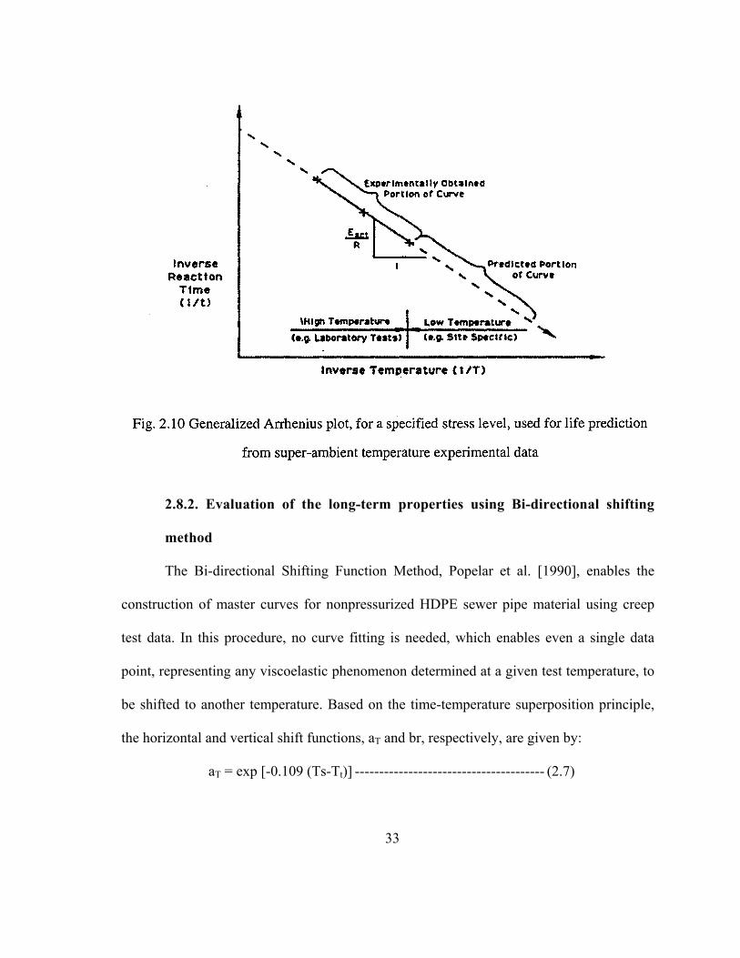
In the Arrhenius plot, degradation is plotted as the logarithm of the reciprocal

of time versus the reciprocal of temperature using Equation 2.6. The schematic of the

plot is provided in Fig. 2.10. It is noted that the temperature has an exponential effect on

the time required for a specified level of degradation based on this model, and the data

used in Equation 2.6 is obtained at a constant level of degradation (indicated by the

modulus decay) in the material. The extrapolation for failure time is similar to that used

in the WLF Method. The WLF and Arrhenius equations are accurate for linear

amorphous polymers, but catastrophic failure that occurs at ductile-brittle transition

makes the prediction difficult for semi-crystalline polymers. This problem should be

addressed, and the life predictions given by the two methods compared, and their

equivalence studied using the procedure developed by Miyano [1996].

43

2.8.2. Evaluation of the long-term properties using Bi-directional shifting

method

The Bi-directional Shifting Function Method, Popelar et al. [1990], enables the

construction of master curves for nonpressurized HDPE sewer pipe material using creep

test data. In this procedure, no curve fitting is needed, which enables even a single data

point, representing any viscoelastic phenomenon determined at a given test temperature, to

be shifted to another temperature. Based on the time-temperature superposition principle,

the horizontal and vertical shift functions, aT and br, respectively, are given by:

aT = exp [-0.109 (Ts-Tt)] --------------------------------------- (2.7)

33

bT= exp [0.0116 (Ts-Tt)] -------------------------------------- (2.8)

where

aT= Time shift function

bT = Stress (or deflection) shift function

Tt = Laboratory test temperature (°C)

TS = Service temperature (°C)

45

CHAPTER 3

EXPERIMENTS

3.1.Introduction

Two types of corrugated HDPE pipe specimens of nominal inside diameters 12

in. (300 mm) were considered. Both types have the same cell classification, i.e. 335420C

with density = 33.97E-3-34.48E-3 lb/in3 (0.941-0.955 g/cm3), melt index=0.4-0.15, flexural

modulus = 110,000-160,000 psi (758-1,103 MPa), tensile strength at yield = 80,000-110,000

psi (552-758 MPa), and Color and UV stabilizer = black with 2% minimum carbon black.

There were small geometrical property differences between the two pipes.

The purpose was to study the changes of diameter and the strains (in function of

time) of Types I and II buried pipes subjected to an AASHTO loading.

The long-term behavior was accelerated with super-ambient temperatures to

provide the data for life prediction (20, 40 and 50 °C).

7.5% vertical deflection is the failure criterion; so, readings have been taken up

to failure or 10, 000 hours.

3.2. Materials and specimen configuration

3.2.1. Specimen details

Cell classification: 335420C

Type of soil: ASTM D2321 Class II, SW/SP, and 90% degree of compaction

46

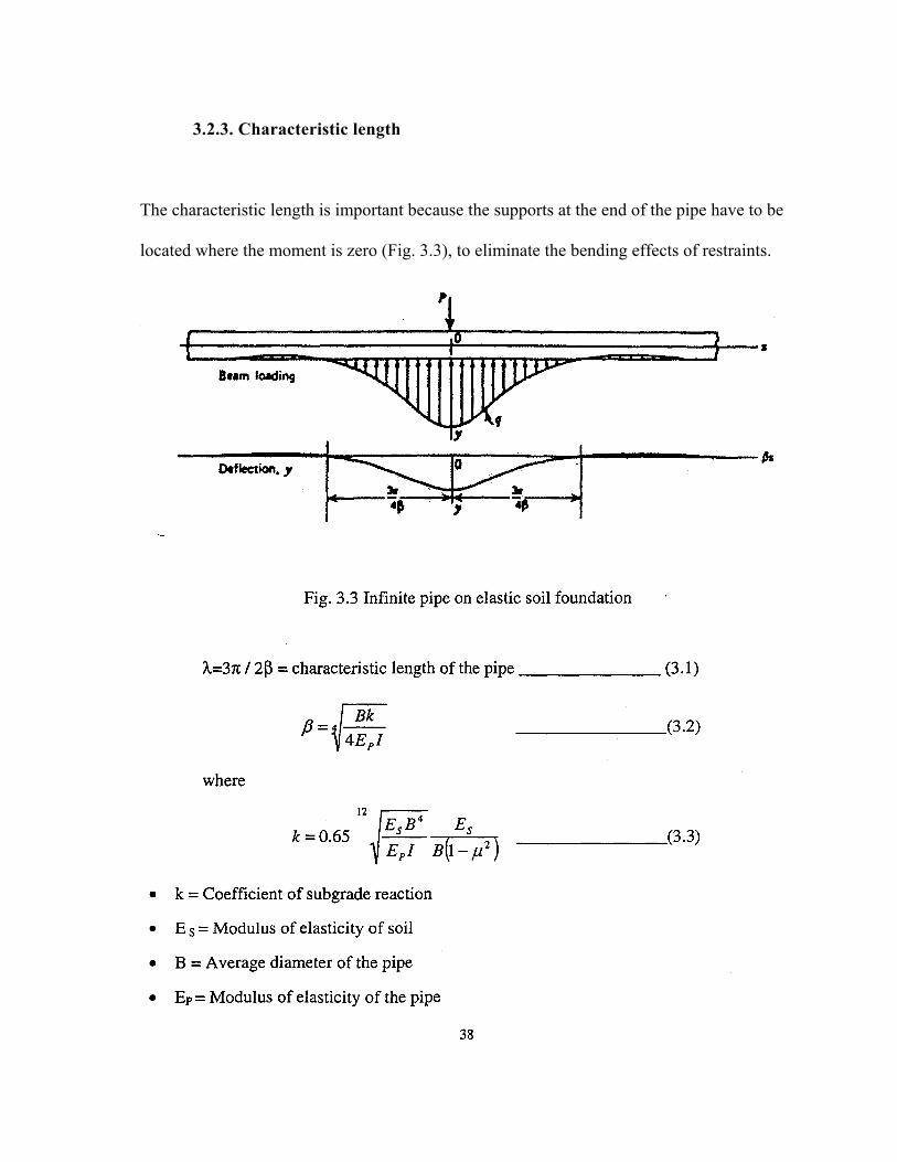
3.2.3. Characteristic length

The characteristic length is important because the supports at the end of the pipe have to be

located where the moment is zero (Fig. 3.3), to eliminate the bending effects of restraints.

µ = Poisson's ratio of soil

I = Moment of inertia of the cross section of the pipe

3.2.4. Minimum cover

The loads on the pipe for minimum cover primarily are due to the surface

loading. A minimum amount of soil cover is needed to spread the surface loading and

to create a more favorable soil pressure distribution around the pipe. Some States

specify their minimum cover requirement according to the type of pavement (rigid or

flexible). Others specify the same minimum cover, and the location to which the cover

is measured (top of the pavement for rigid pavements and top of the subgrade for

flexible pavements). Minimum cover requirements are listed in Table 3.1 [CPPA, 96].

39

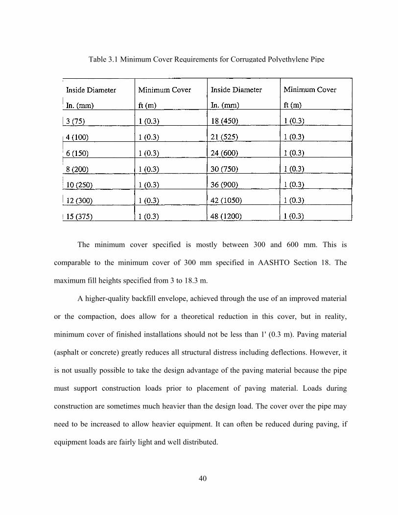
Table 3.1 Minimum Cover Requirements for Corrugated Polyethylene Pipe

The minimum cover specified is mostly between 300 and 600 mm. This is

comparable to the minimum cover of 300 mm specified in AASHTO Section 18. The

maximum fill heights specified from 3 to 18.3 m.

A higher-quality backfill envelope, achieved through the use of an improved material

or the compaction, does allow for a theoretical reduction in this cover, but in reality,

minimum cover of finished installations should not be less than 1' (0.3 m). Paving material

(asphalt or concrete) greatly reduces all structural distress including deflections. However, it

is not usually possible to take the design advantage of the paving material because the pipe

must support construction loads prior to placement of paving material. Loads during

construction are sometimes much heavier than the design load. The cover over the pipe may

need to be increased to allow heavier equipment. It can often be reduced during paving, if

equipment loads are fairly light and well distributed.

40

According to Katona (1995), currently, the tentative guideline for minimum cover of

plastic pipe, as suggested by the AASHTO Flexible Culvert Committee, is taken directly

from the metal culvert industry, the American Iron and Steel Institute (AISI). The AISI

specification for corrugated metal culverts requires a minimum of 12 in., cover owing to

the concern due to construction loads prior to paving. Corrugated plastic pipes are

considerably more flexible in ovaling deformation than are typical corrugated steel pipes

of the same diameter. Consequently, the minimum 12 in. cover is more than adequate for

plastic pipe.

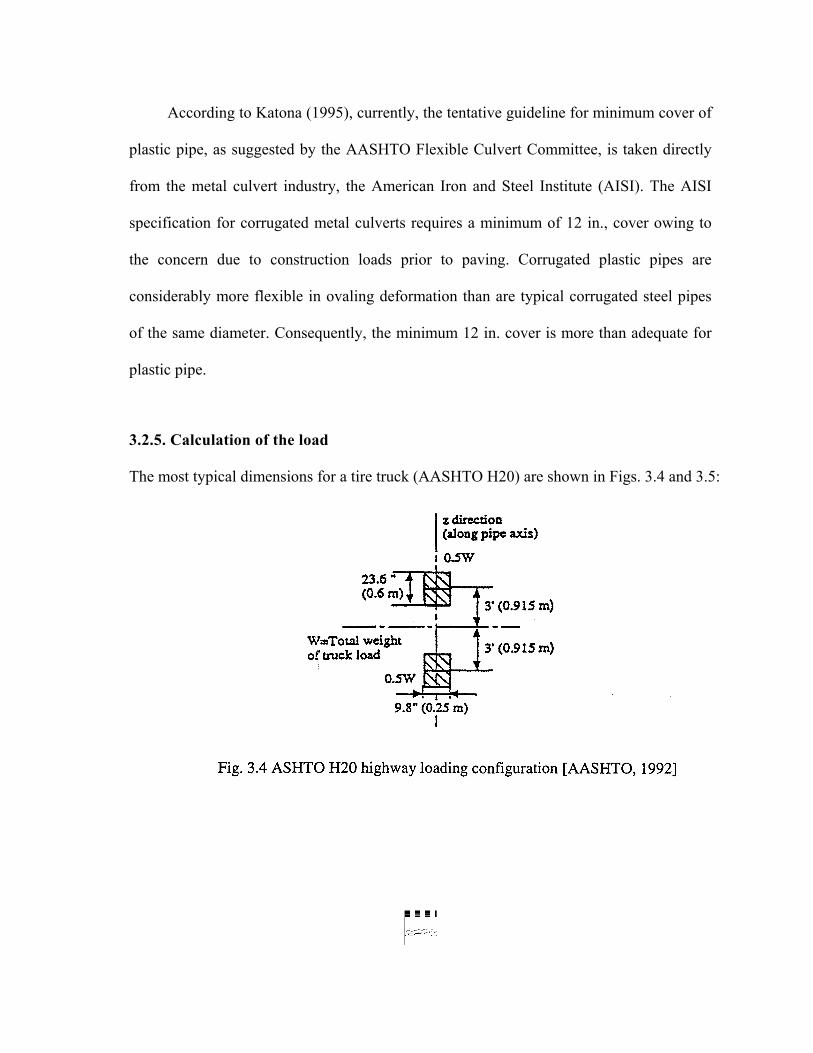
3.2.5. Calculation of the load

The most typical dimensions for a tire truck (AASHTO H20) are shown in Figs. 3.4 and 3.5:

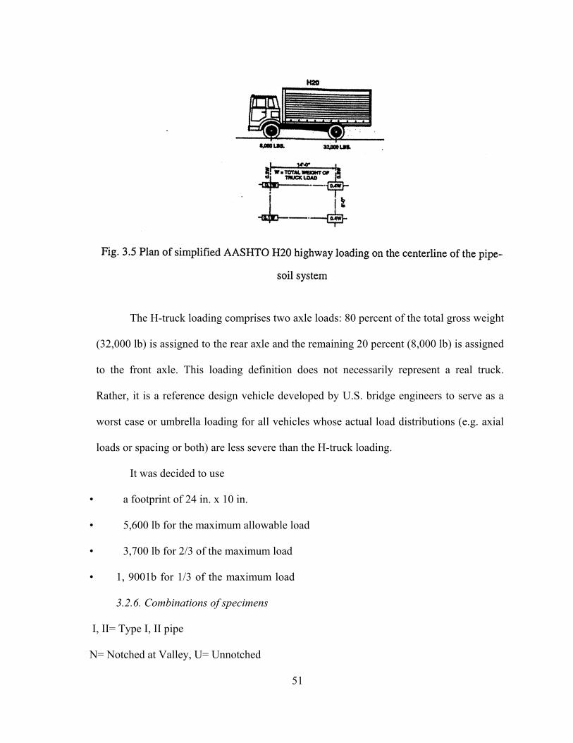
The H-truck loading comprises two axle loads: 80 percent of the total gross weight

(32,000 lb) is assigned to the rear axle and the remaining 20 percent (8,000 lb) is assigned

to the front axle. This loading definition does not necessarily represent a real truck.

Rather, it is a reference design vehicle developed by U.S. bridge engineers to serve as a

worst case or umbrella loading for all vehicles whose actual load distributions (e.g. axial

loads or spacing or both) are less severe than the H-truck loading.

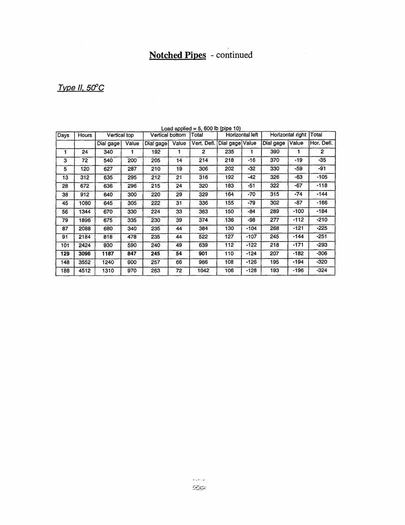
It was decided to use

• a footprint of 24 in. x 10 in.

• 5,600 lb for the maximum allowable load

• 3,700 lb for 2/3 of the maximum load

• 1, 9001b for 1/3 of the maximum load

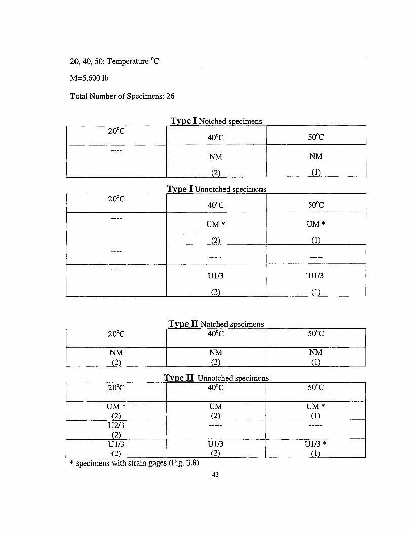
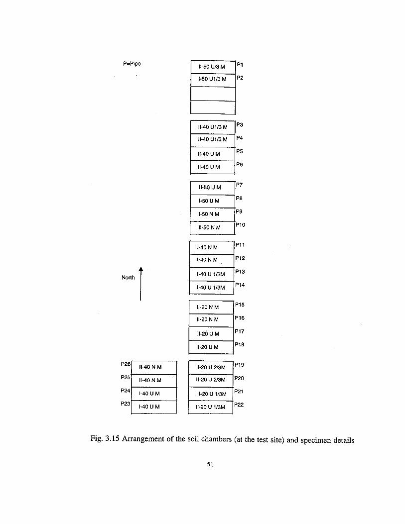
3.2.6. Combinations of specimens

I, II= Type I, II pipe

N= Notched at Valley, U= Unnotched

51

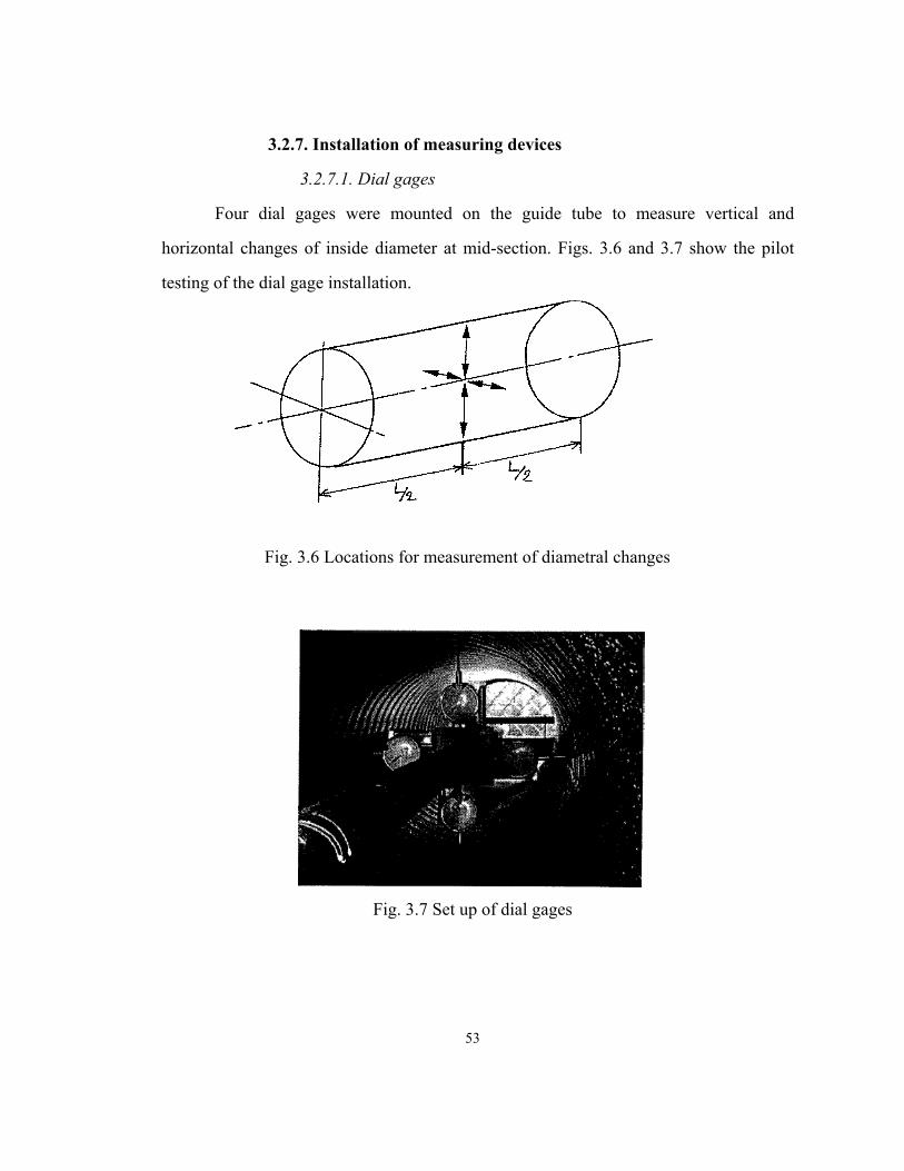
3.2.7. Installation of measuring devices

3.2.7.1. Dial gages

Four dial gages were mounted on the guide tube to measure vertical and

horizontal changes of inside diameter at mid-section. Figs. 3.6 and 3.7 show the pilot

testing of the dial gage installation.

Fig. 3.6 Locations for measurement of diametral changes

Fig. 3.7 Set up of dial gages

53

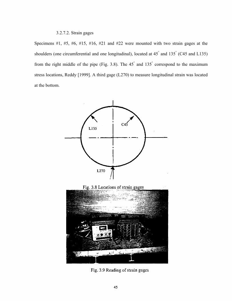
3.2.7.2. Strain gages

Specimens #1, #5, #6, #15, #16, #21 and #22 were mounted with two strain gages at the

shoulders (one circumferential and one longitudinal), located at 45° and 135° (C45 and L135)

from the right middle of the pipe (Fig. 3.8). The 45° and 135° correspond to the maximum

stress locations, Reddy [1999]. A third gage (L270) to measure longitudinal strain was located

at the bottom.

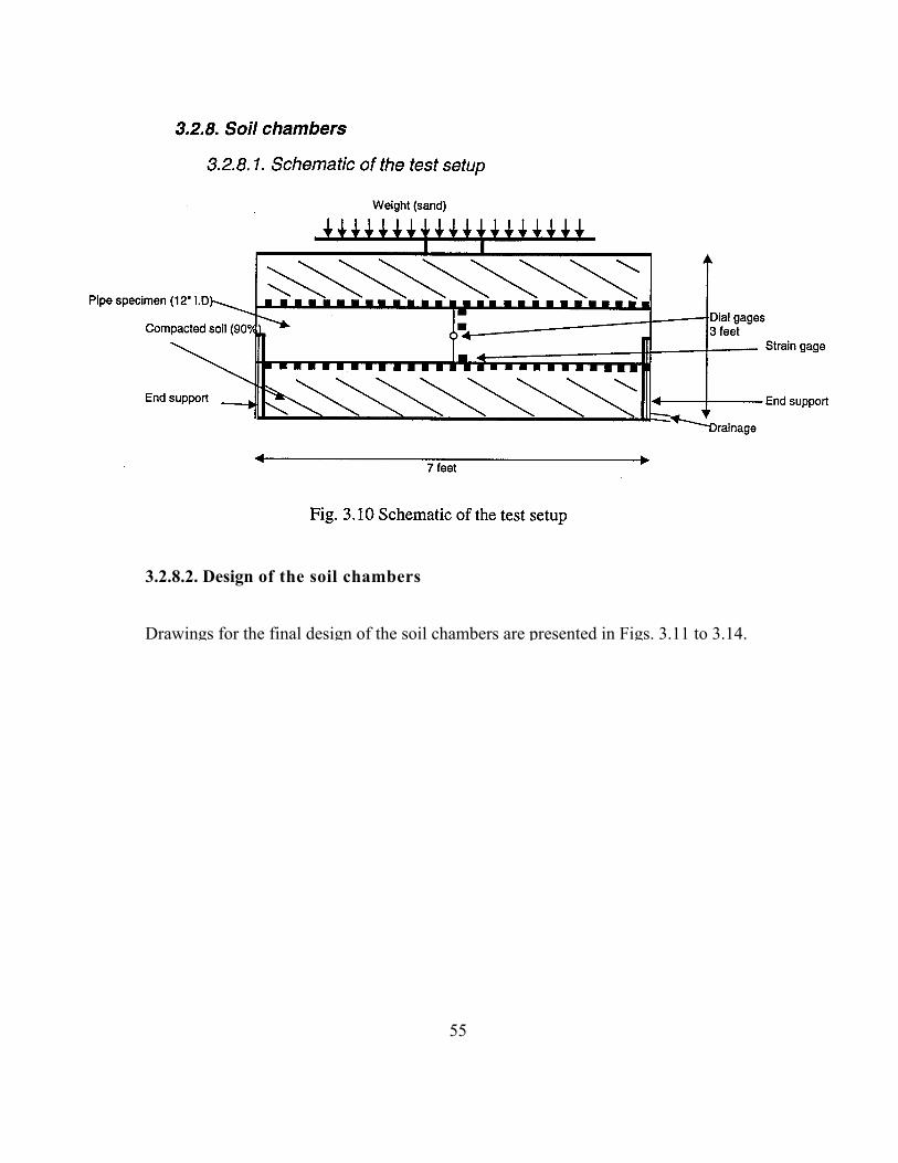
3.2.8.2. Design of the soil chambers

Drawings for the final design of the soil chambers are presented in Figs. 3.11 to 3.14.

55

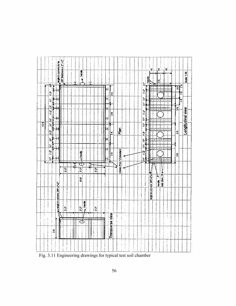
Fig. 3.11 Engineering drawings for typical test soil chamber

56

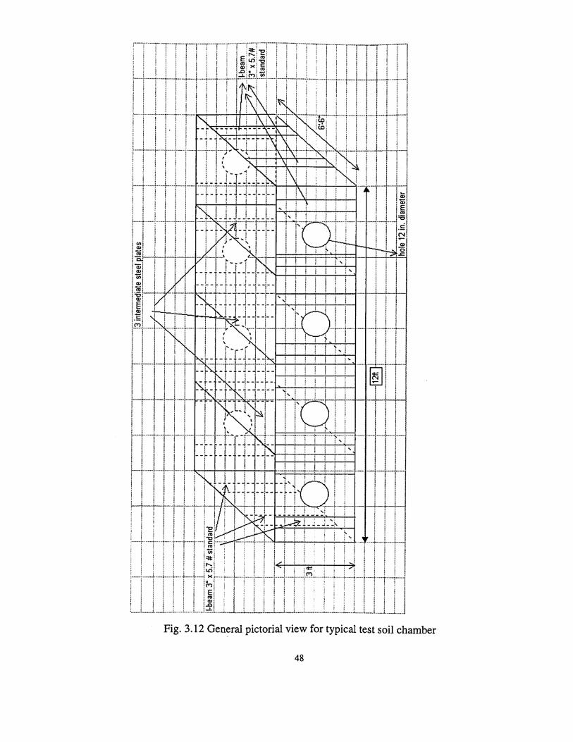
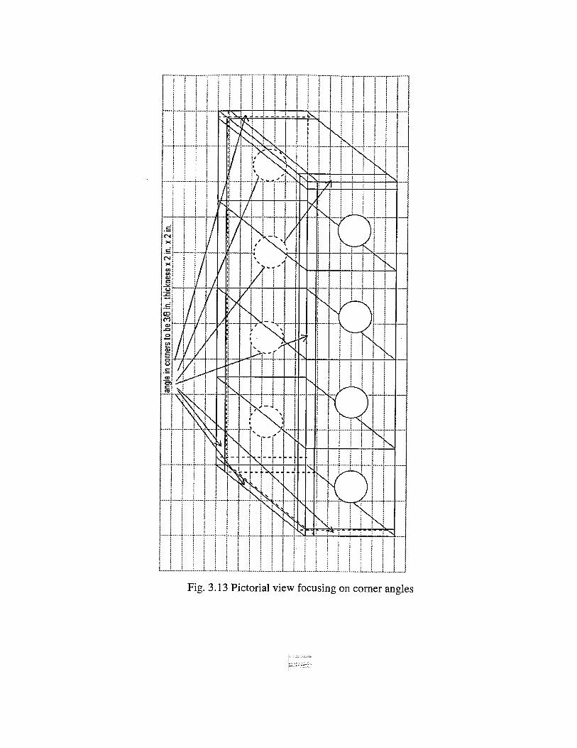
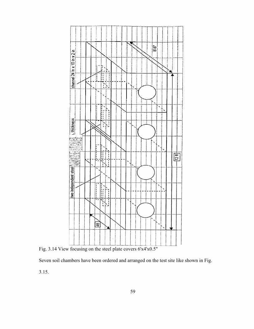
Fig. 3.14 View focusing on the steel plate covers 6'x4'x0.5"

Seven soil chambers have been ordered and arranged on the test site like shown in Fig.

3.15.

59

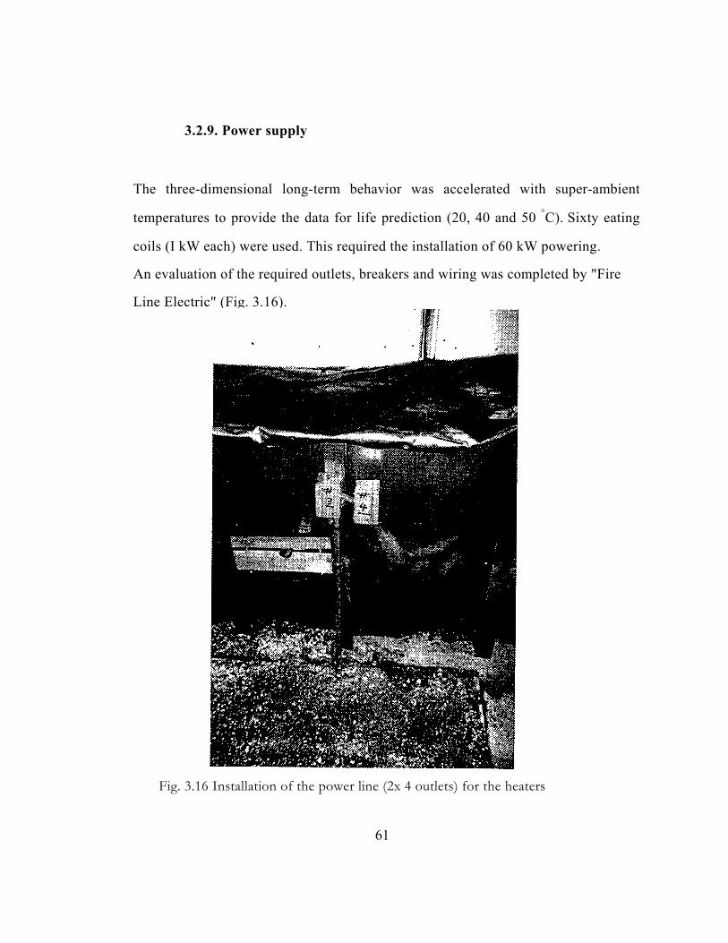
3.2.9. Power supply

The three-dimensional long-term behavior was accelerated with super-ambient

temperatures to provide the data for life prediction (20, 40 and 50 °C). Sixty eating

coils (I kW each) were used. This required the installation of 60 kW powering.

An evaluation of the required outlets, breakers and wiring was completed by "Fire

Line Electric" (Fig. 3.16).

Fig. 3.16 Installation of the power line (2x 4 outlets) for the heaters

61

Six heaters were installed for each of the specimens #1, #2, #7, #8, #9 and #10. The

arrows show the locations of the heaters in Fig. 3.17. Each heater is one-inch

diameter and 15 in. long.

3.3. Performance of buried pipe, subjected to live load

3.3.1. Fabrication and installation of soil chambers

The steel soil chambers were made by the company "Sun Metal" at Pompano

Beach. A crane was used to set up the soil chambers, as shown on Figs. 3.18 and 3.19.

The weight of chamber block with four soil chambers was 5,000 lb

62

Fig. 3.18 Delivery of soil chambers

Fig. 3.19 Set up of soil chambers

63

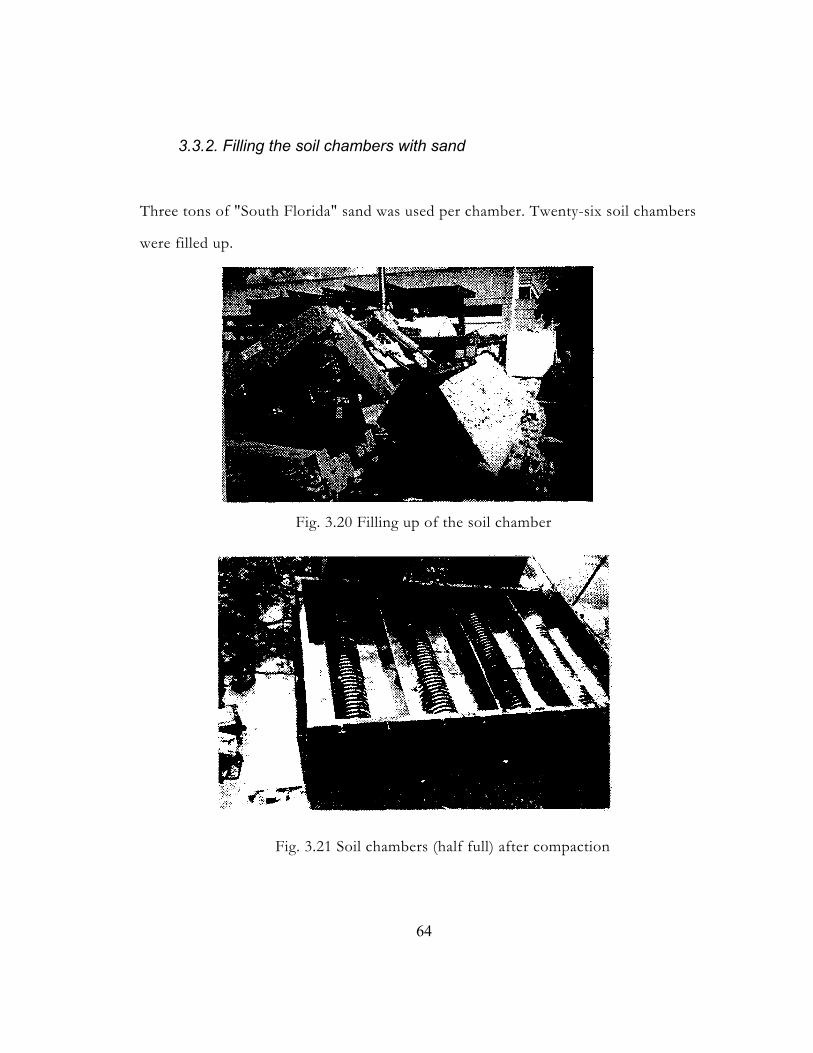
3.3.2. Filling the soil chambers with sand

Three tons of "South Florida" sand was used per chamber. Twenty-six soil chambers

were filled up.

Fig. 3.20 Filling up of the soil chamber

Fig. 3.21 Soil chambers (half full) after compaction

64

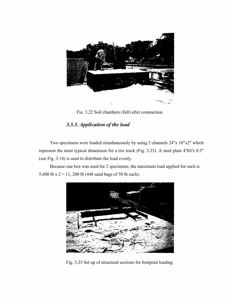
Fig. 3.22 Soil chambers (full) after compaction

3.3.3. Application of the load

Two specimens were loaded simultaneously by using 2 channels 24"x 10"x2" which

represent the most typical dimension for a tire truck (Fig. 3.23). A steel plate 4'X6'x 0.5"

(see Fig. 3.14) is used to distribute the load evenly.

Because one box was used for 2 specimens, the maximum load applied for each is

5,600 lb x 2 = 11, 200 lb (448 sand bags of 50 lb each).

Fig. 3.23 Set up of structural sections for footprint loading

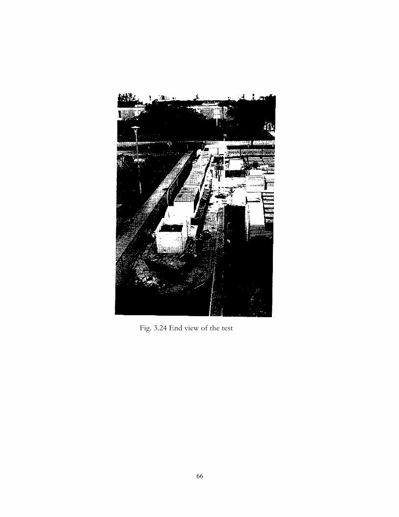
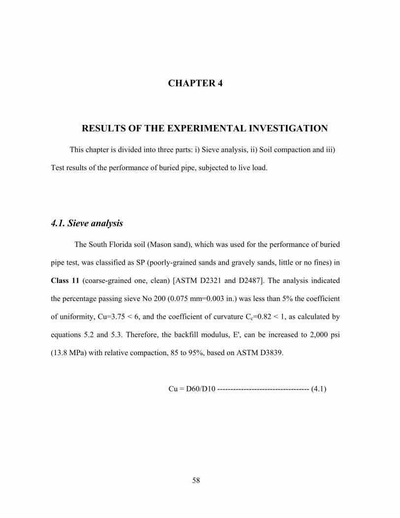
Fig. 3.24 End view of the test

66

CHAPTER 4

RESULTS OF THE EXPERIMENTAL INVESTIGATION

This chapter is divided into three parts: i) Sieve analysis, ii) Soil compaction and iii)

Test results of the performance of buried pipe, subjected to live load.

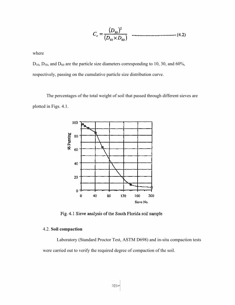
4.1. Sieve analysis

The South Florida soil (Mason sand), which was used for the performance of buried

pipe test, was classified as SP (poorly-grained sands and gravely sands, little or no fines) in

Class 11 (coarse-grained one, clean) [ASTM D2321 and D2487]. The analysis indicated

the percentage passing sieve No 200 (0.075 mm=0.003 in.) was less than 5% the coefficient

of uniformity, Cu=3.75 < 6, and the coefficient of curvature Cc=0.82 < 1, as calculated by

equations 5.2 and 5.3. Therefore, the backfill modulus, E', can be increased to 2,000 psi

(13.8 MPa) with relative compaction, 85 to 95%, based on ASTM D3839.

Cu = D60/D10 ----------------------------------- (4.1)

58

where

D10, D30, and D60 are the particle size diameters corresponding to 10, 30, and 60%,

respectively, passing on the cumulative particle size distribution curve.

The percentages of the total weight of soil that passed through different sieves are

plotted in Figs. 4.1.

4.2. Soil compaction

Laboratory (Standard Proctor Test, ASTM D698) and in-situ compaction tests

were carried out to verify the required degree of compaction of the soil.

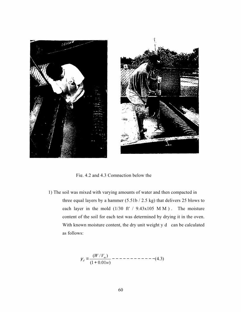
Fig. 4.2 and 4.3 Compaction below the

1) The soil was mixed with varying amounts of water and then compacted in

three equal layers by a hammer (5.51b / 2.5 kg) that delivers 25 blows to

each layer in the mold (1/30 ft' / 9.43x105 M M ) . The moisture

content of the soil for each test was determined by drying it in the oven.

With known moisture content, the dry unit weight y d can be calculated

as follows:

)3.4()01.01(

)/( −−−−−−−−−−−−+

=w

VW mdγ

60

where γd =dry unit weight

W = weight of compacted soil in the mold

Vm= volume of the mold

w = moisture content (%)

2) In-situ compactions of the soil in bedding, haunch, and backfill zones in the

chamber were carried out by using a compactor tool (Figs. 4.2 and 4.3) after

the mold was buried. The molds were carefully taken out after proper

compaction process and the moisture contents and dry unit weights of the

samples found in a similar manner to that for the standard compaction test.

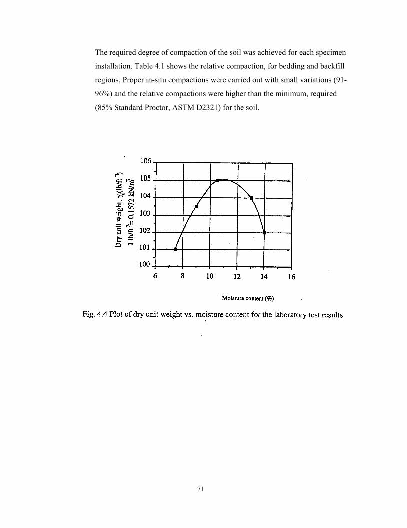
Laboratory Standard Proctor Tests were carried out prior to the in-situ

compaction tests and the relationship between dry unit weight and moisture

content the soil was evaluated Fig. 4.4. It was found that the maximum dry

unit weight was 1051b / ft3 with the optimum moisture content 10.5%.

Based on the laboratory and in-situ test results, the degree of compaction

can be determined as follows:

where R = relative compaction

γd(in-situ) = dry unit weight of in-situ-sample

γd(max-lab)=maximum dry unit weight, obtained in the laboratory

70

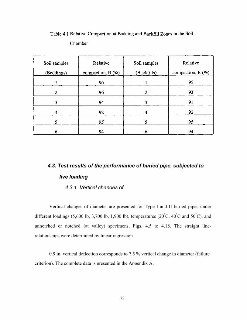
The required degree of compaction of the soil was achieved for each specimen

installation. Table 4.1 shows the relative compaction, for bedding and backfill

regions. Proper in-situ compactions were carried out with small variations (91-

96%) and the relative compactions were higher than the minimum, required

(85% Standard Proctor, ASTM D2321) for the soil.

71

4.3. Test results of the performance of buried pipe, subjected to

live loading

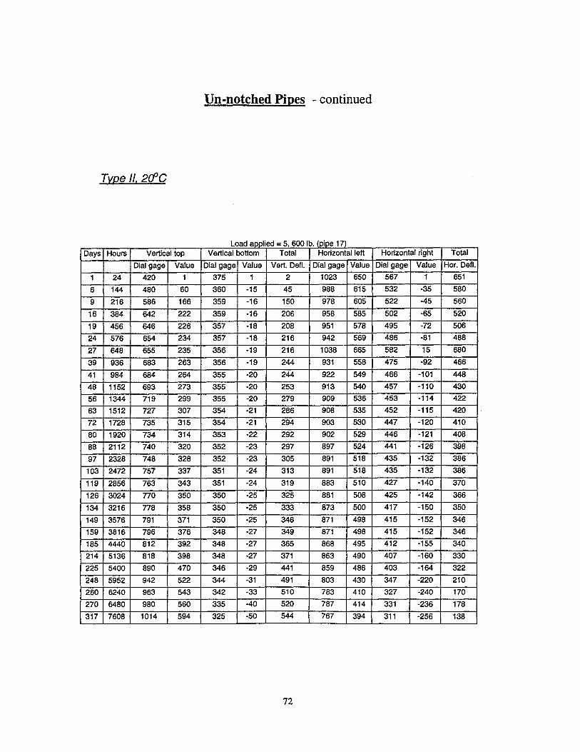
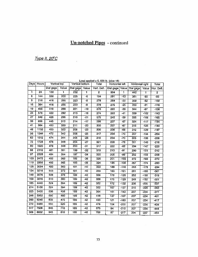
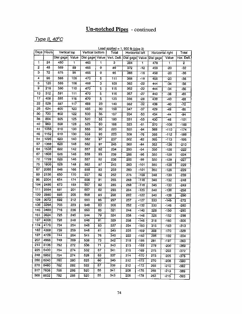
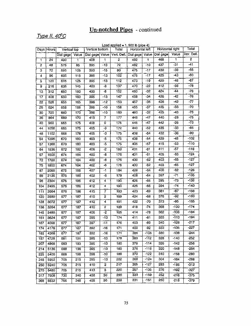
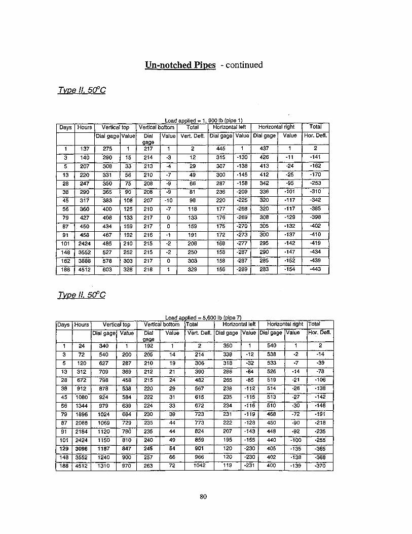
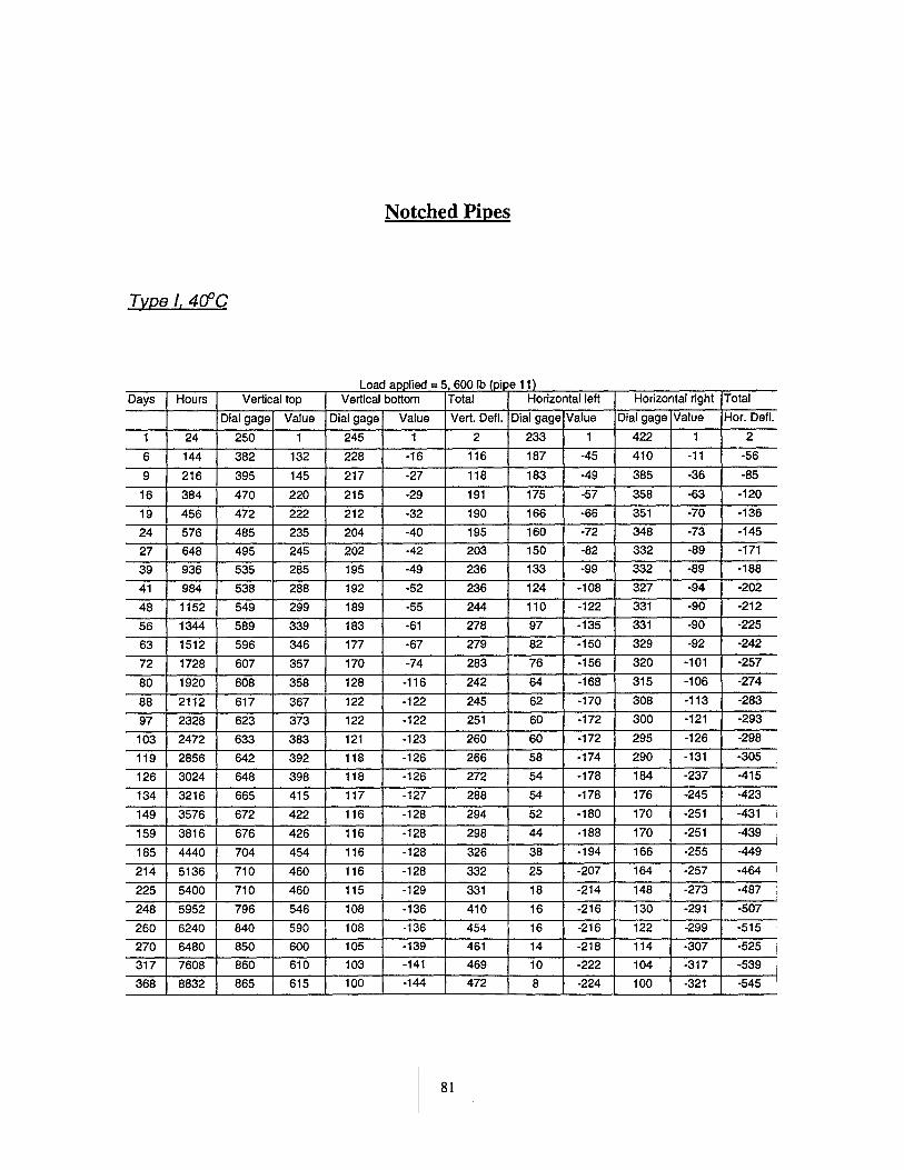
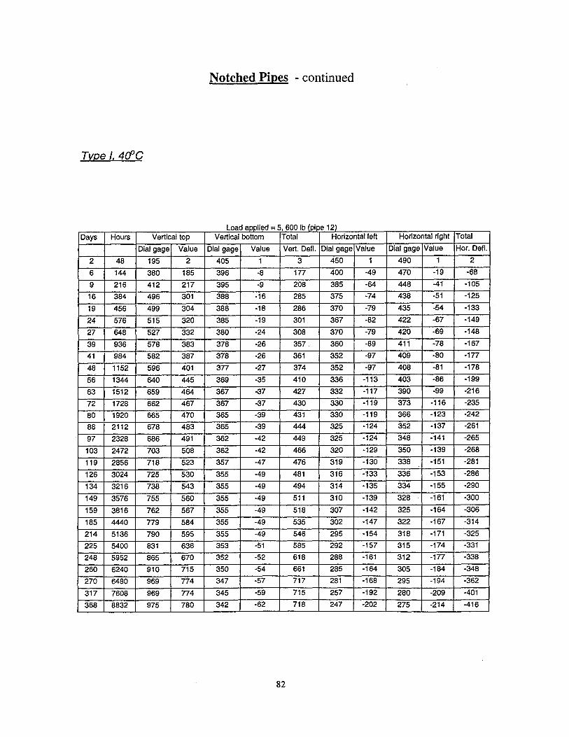
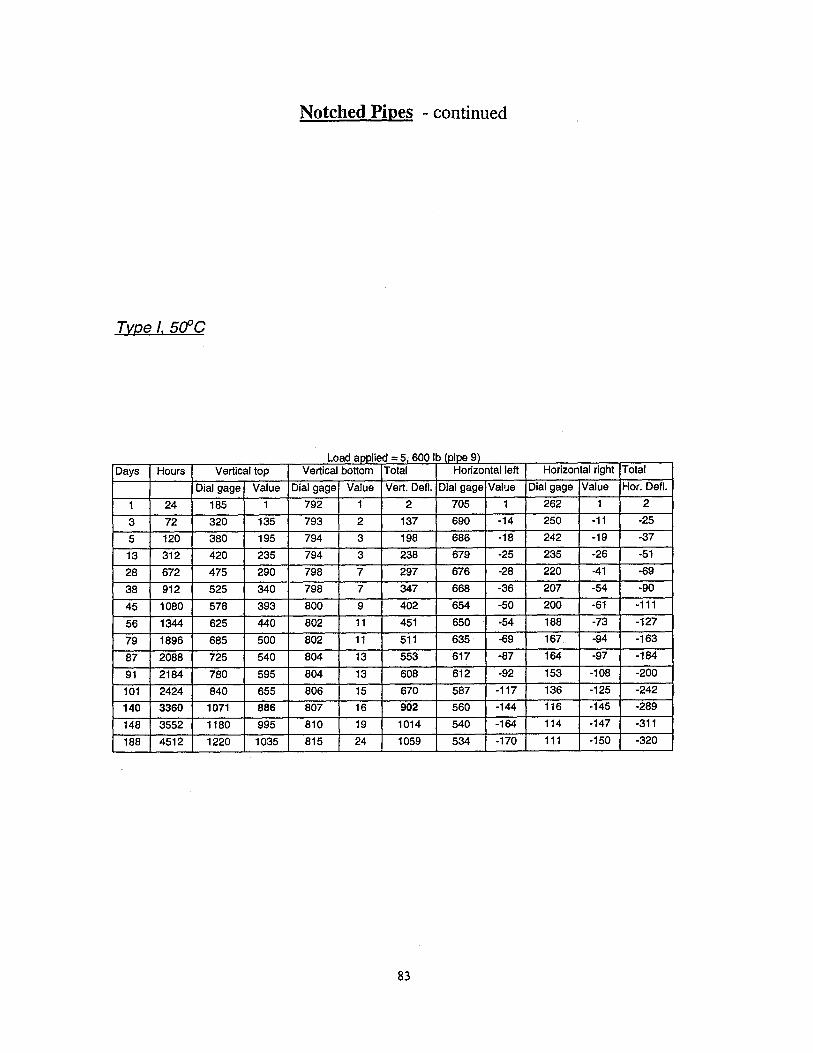
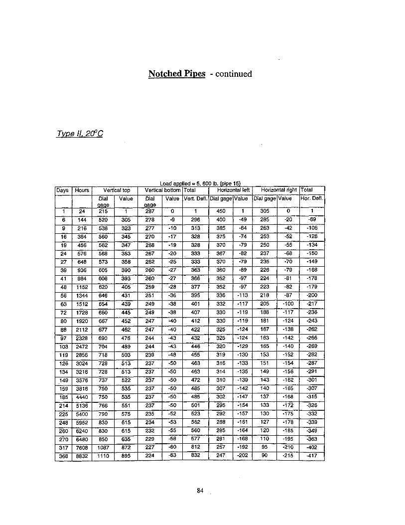
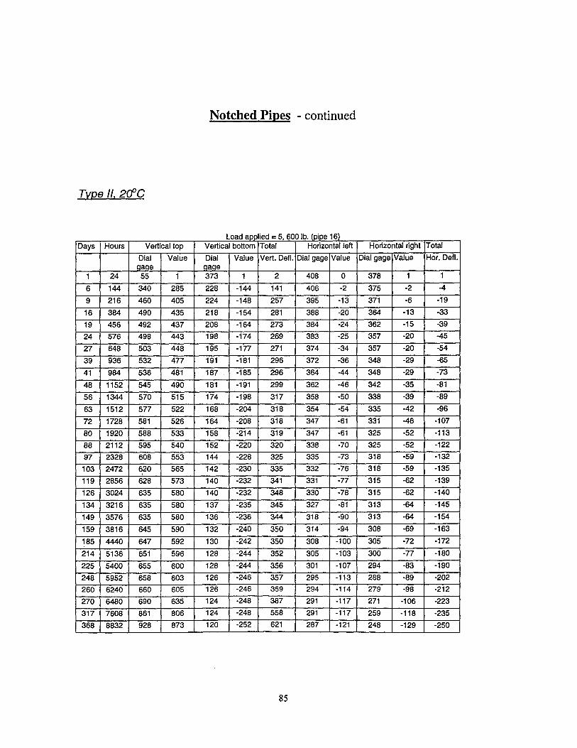
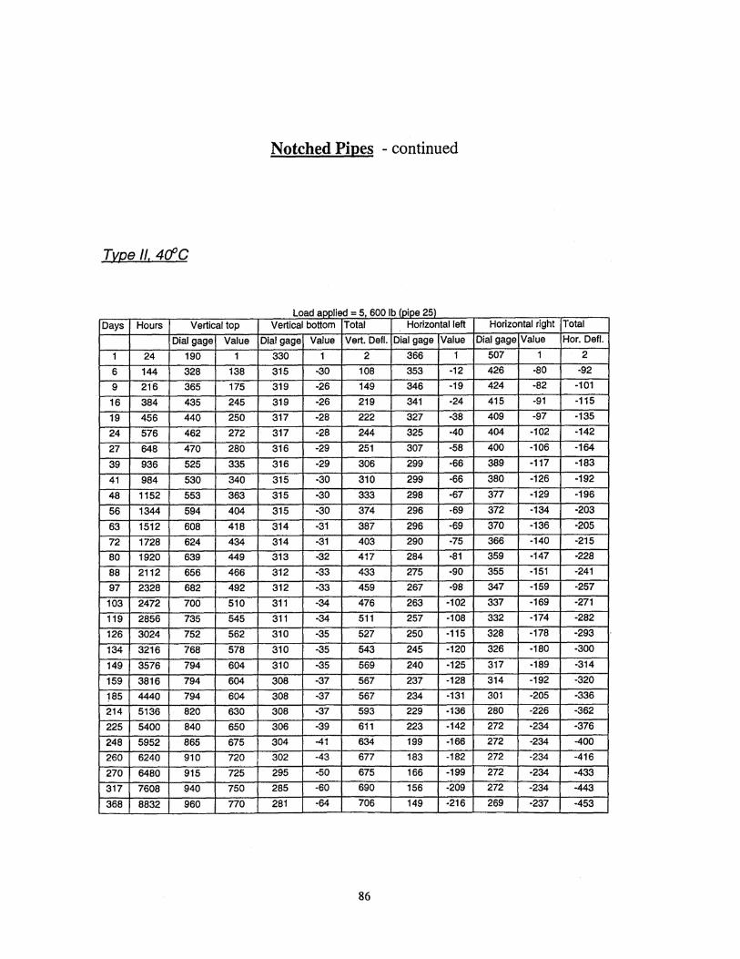
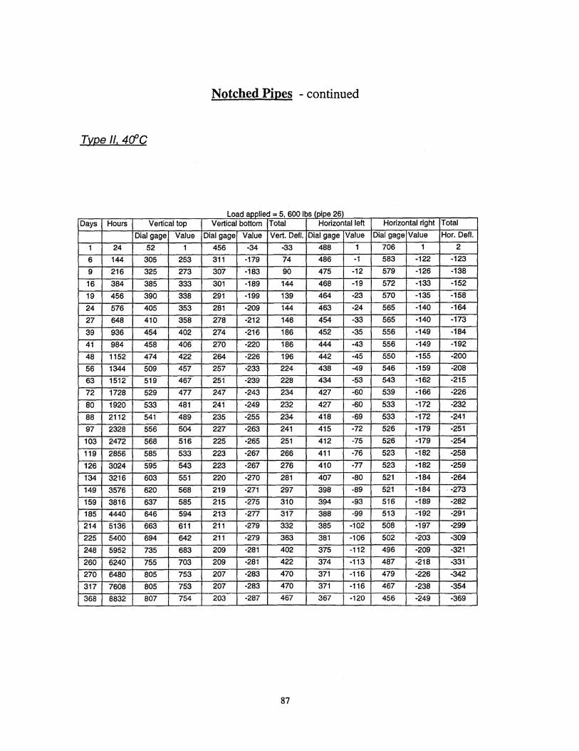
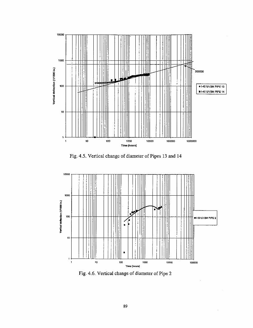
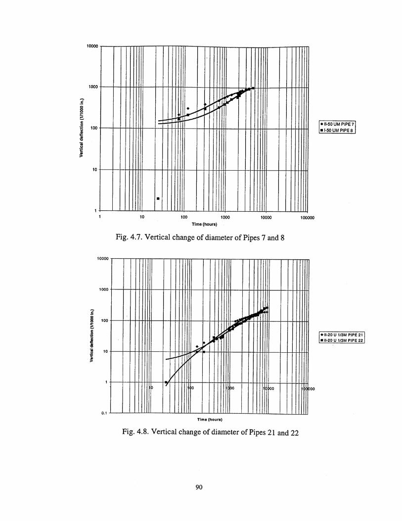
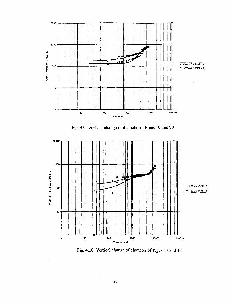
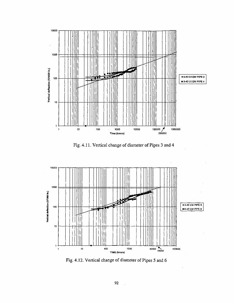
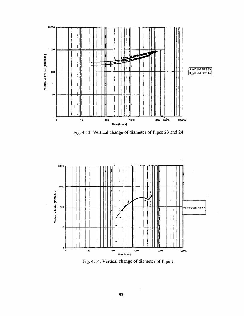
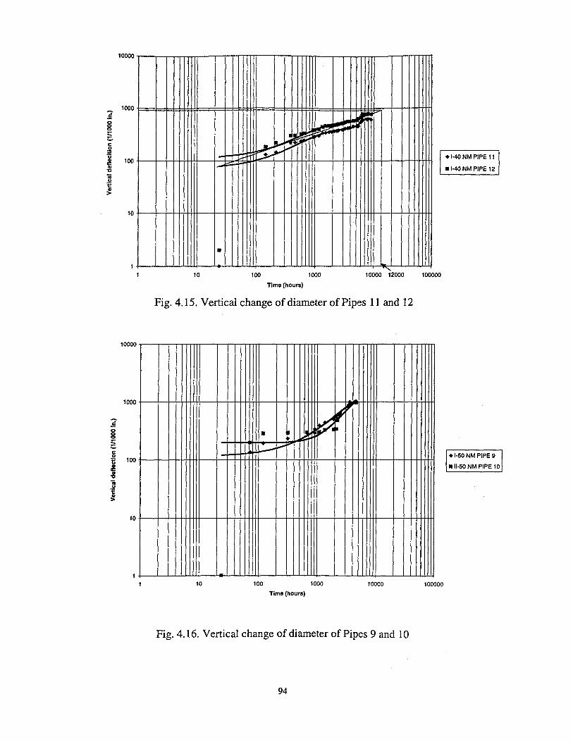
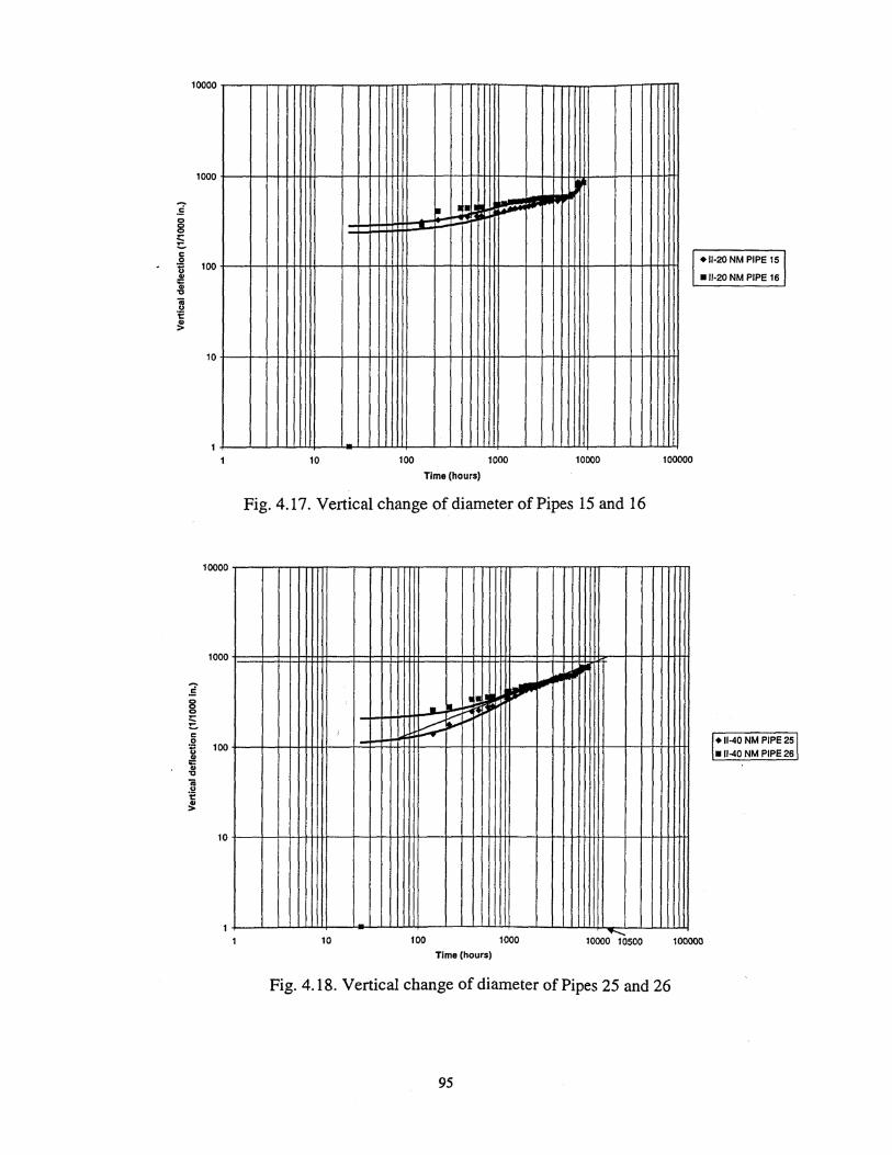
4.3.1. Vertical changes of

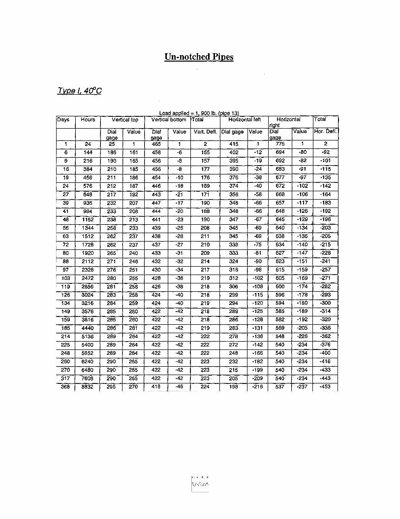
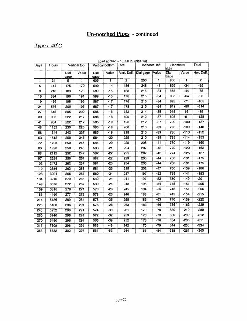
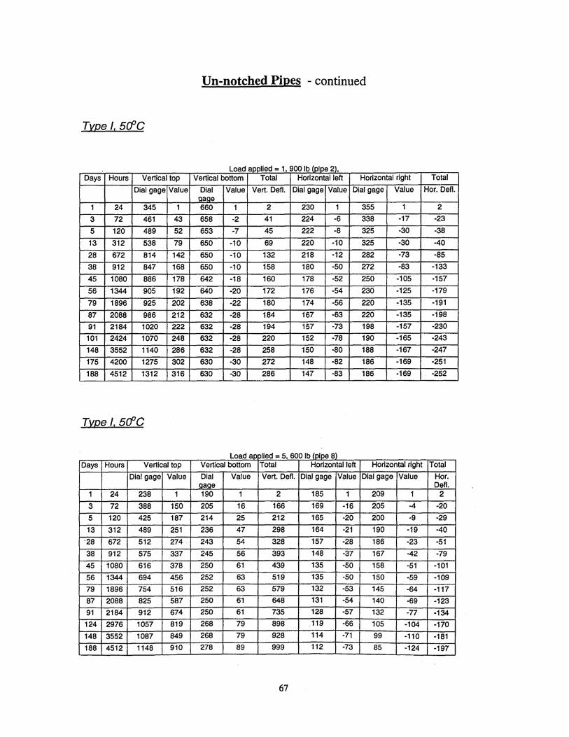
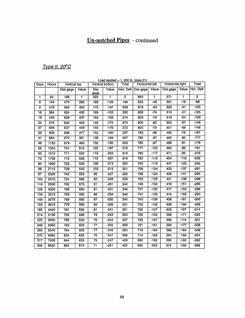
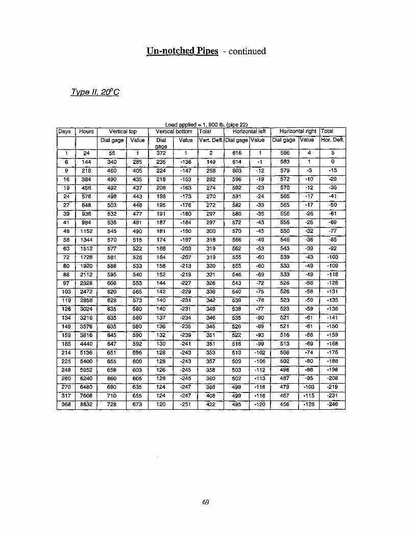
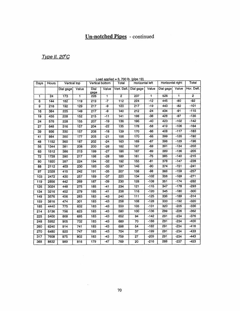
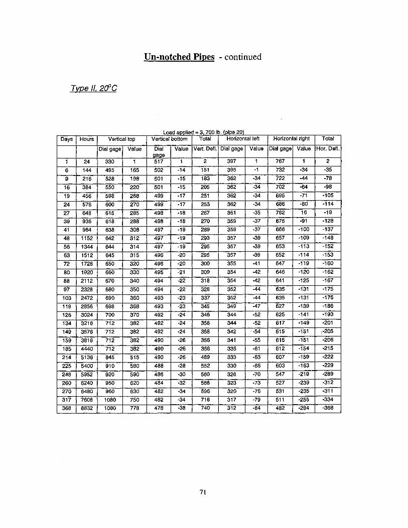
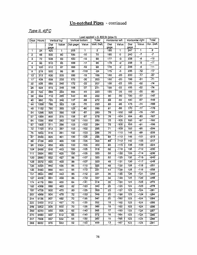
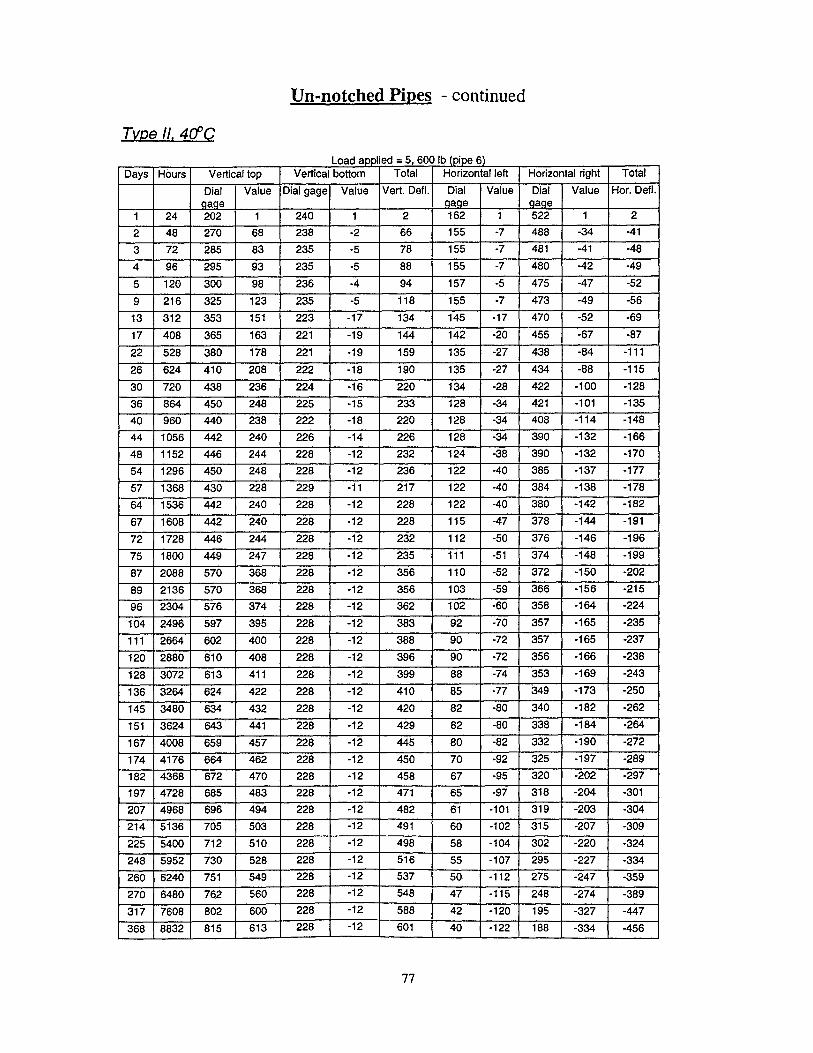
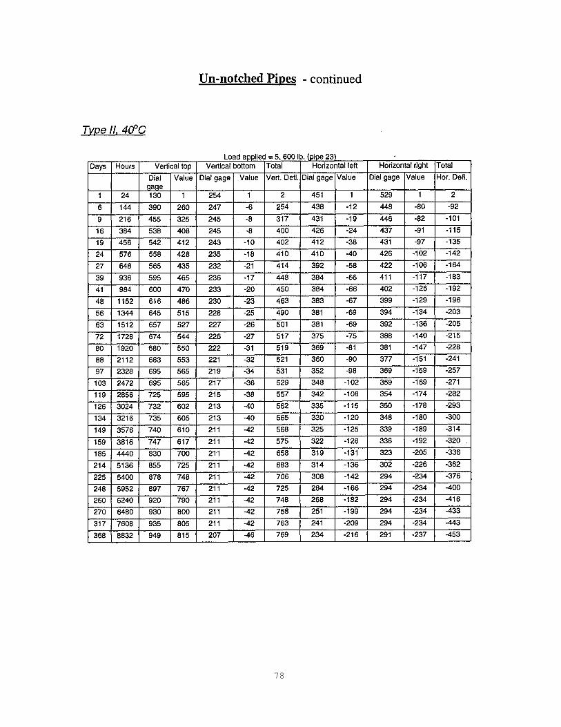
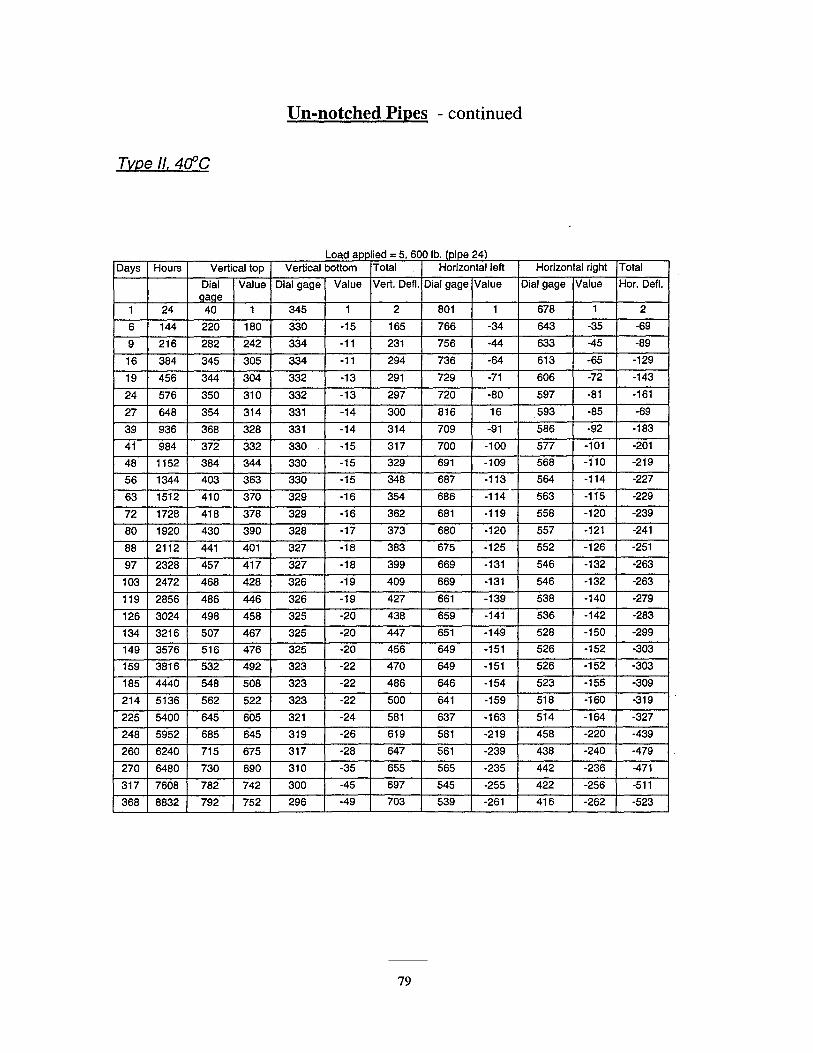
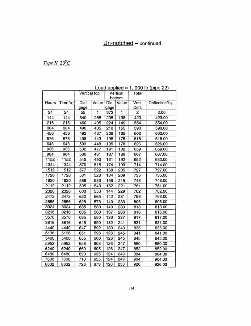
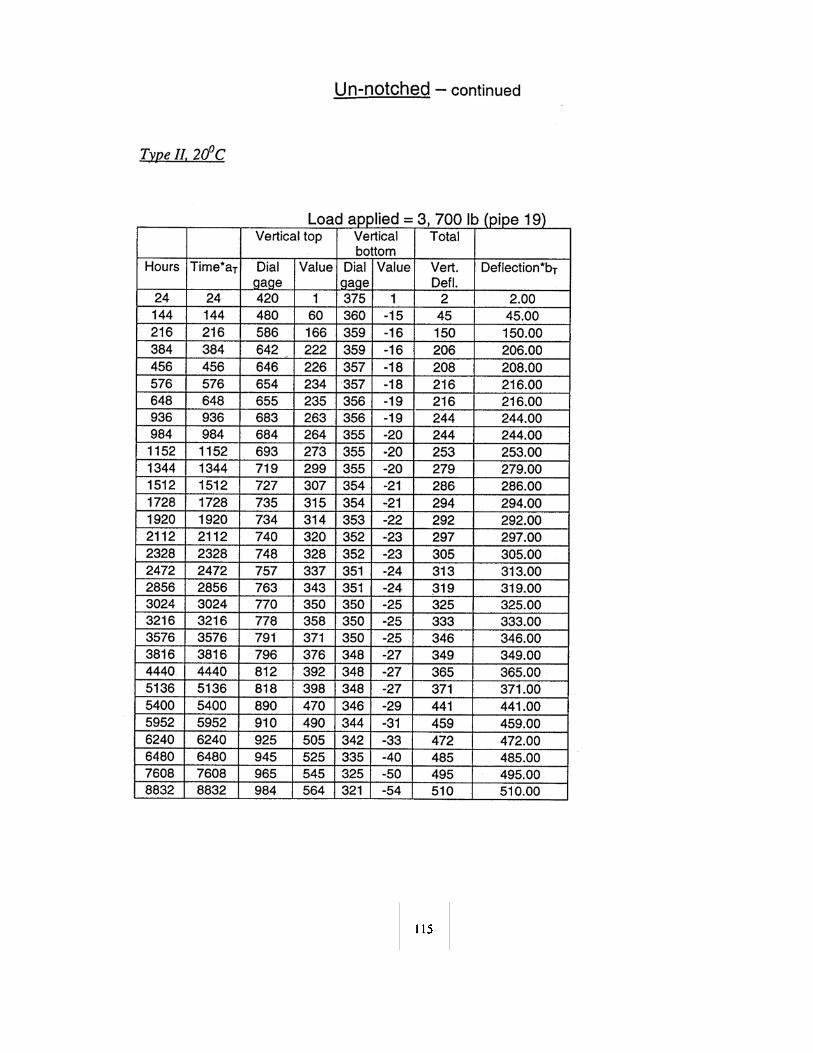
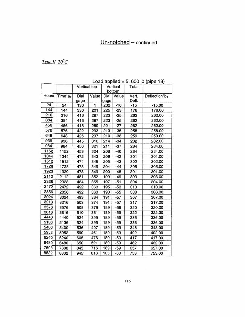
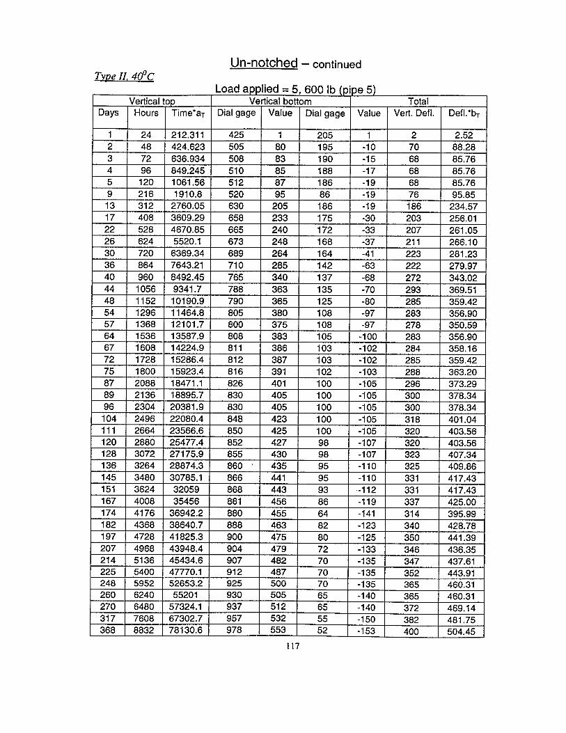
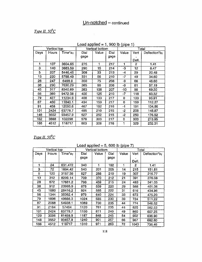
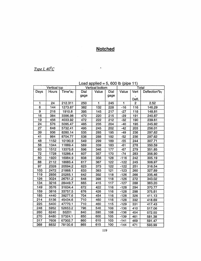
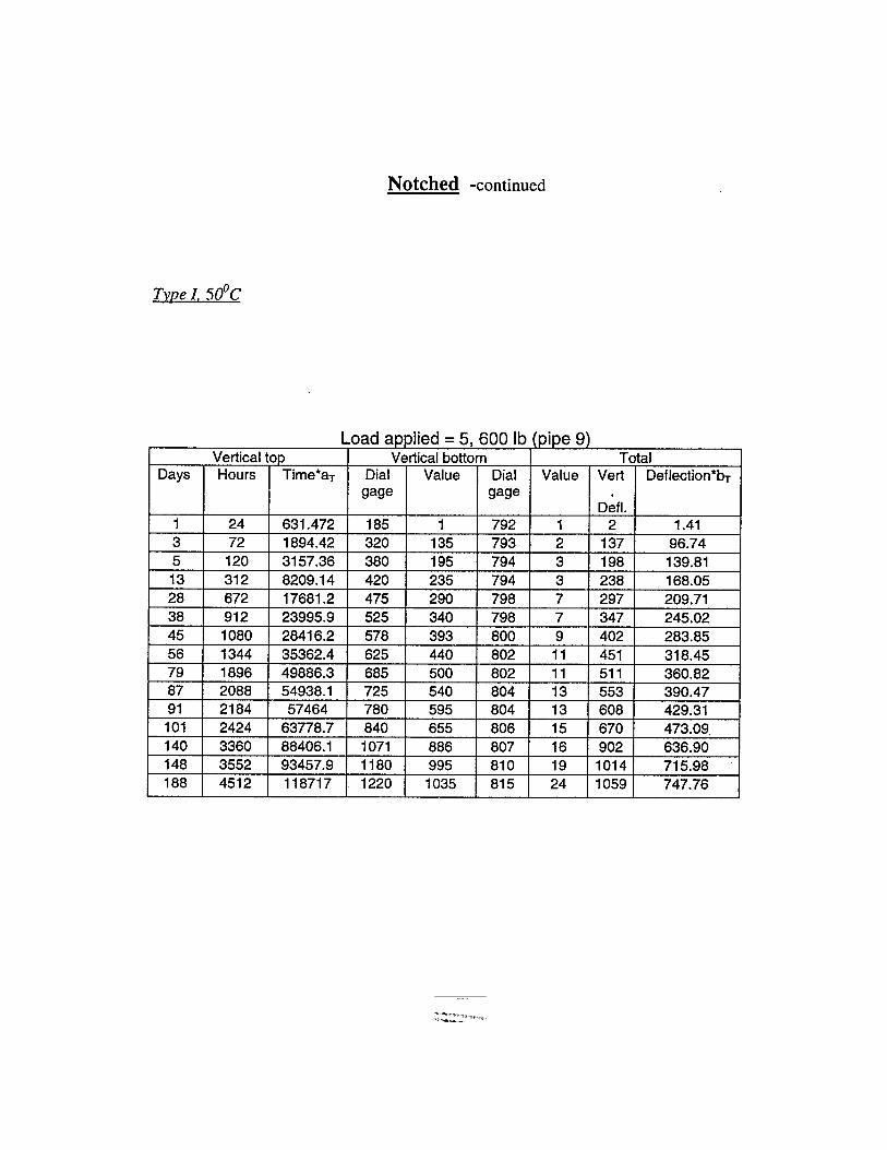
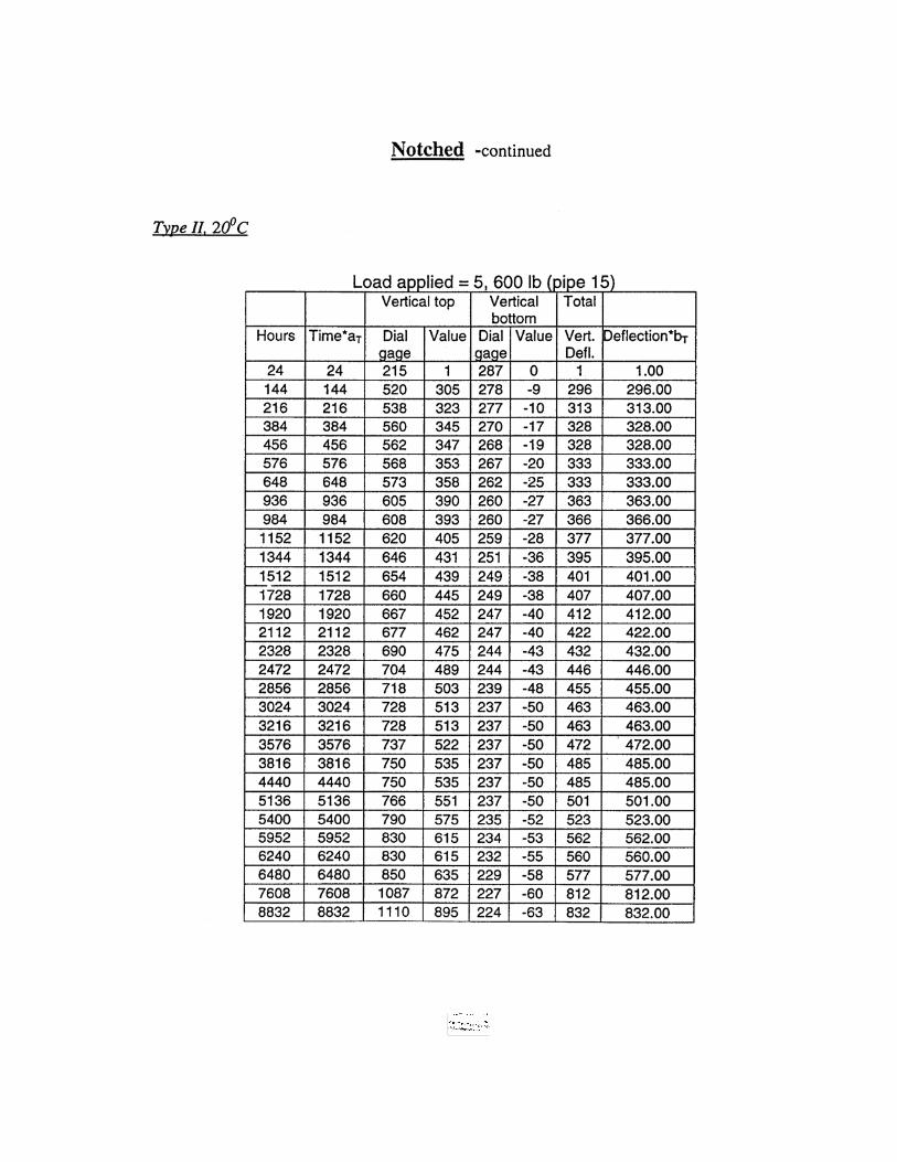
Vertical changes of diameter are presented for Type I and II buried pipes under

different loadings (5,600 lb, 3,700 lb, 1,900 lb), temperatures (20°C, 40°C and 50°C), and

unnotched or notched (at valley) specimens, Figs. 4.5 to 4.18. The straight line-

relationships were determined by linear regression.

0.9 in. vertical deflection corresponds to 7.5 % vertical change in diameter (failure

criterion). The complete data is presented in the Appendix A.

72

APPENDIX A Deflection Data for Notched and Un-notched Pipes

Deflections (1/1000 in.)

73

78

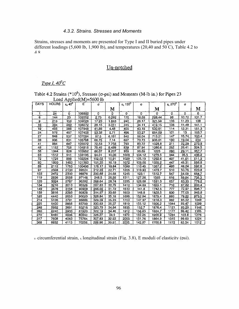
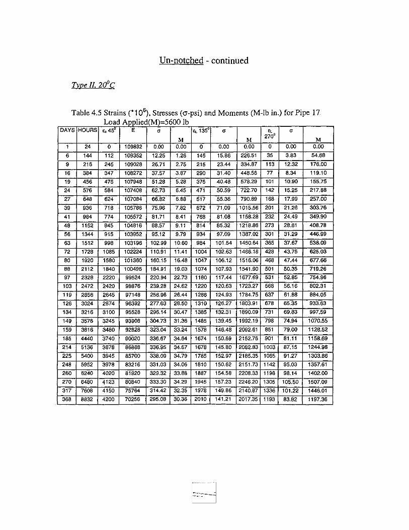
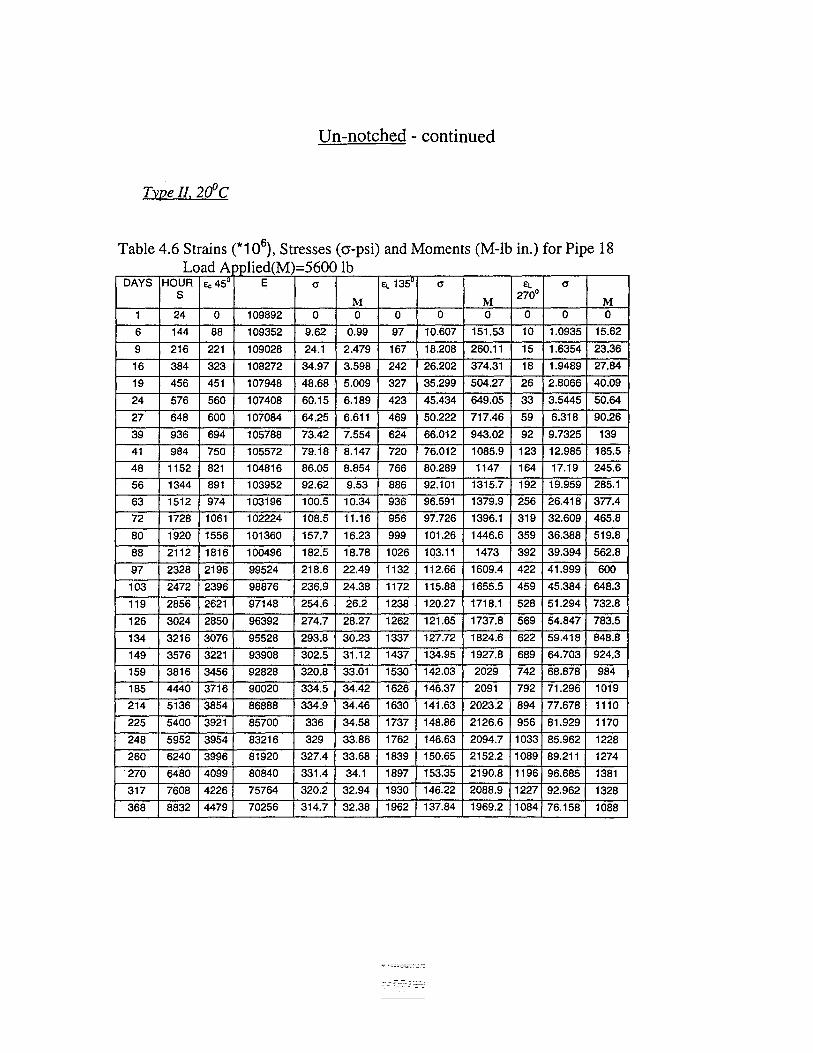
4.3.2. Strains, Stresses and Moments

Strains, stresses and moments are presented for Type I and II buried pipes under different loadings (5,600 lb, 1,900 lb), and temperatures (20,40 and 50°C), Table 4.2 to 4 8

E~ circumferential strain, E, longitudinal strain (Fig. 3.8), E moduli of elasticity (psi).

96

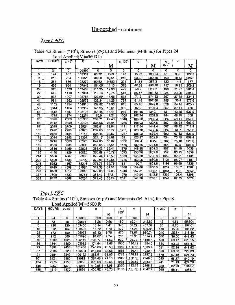
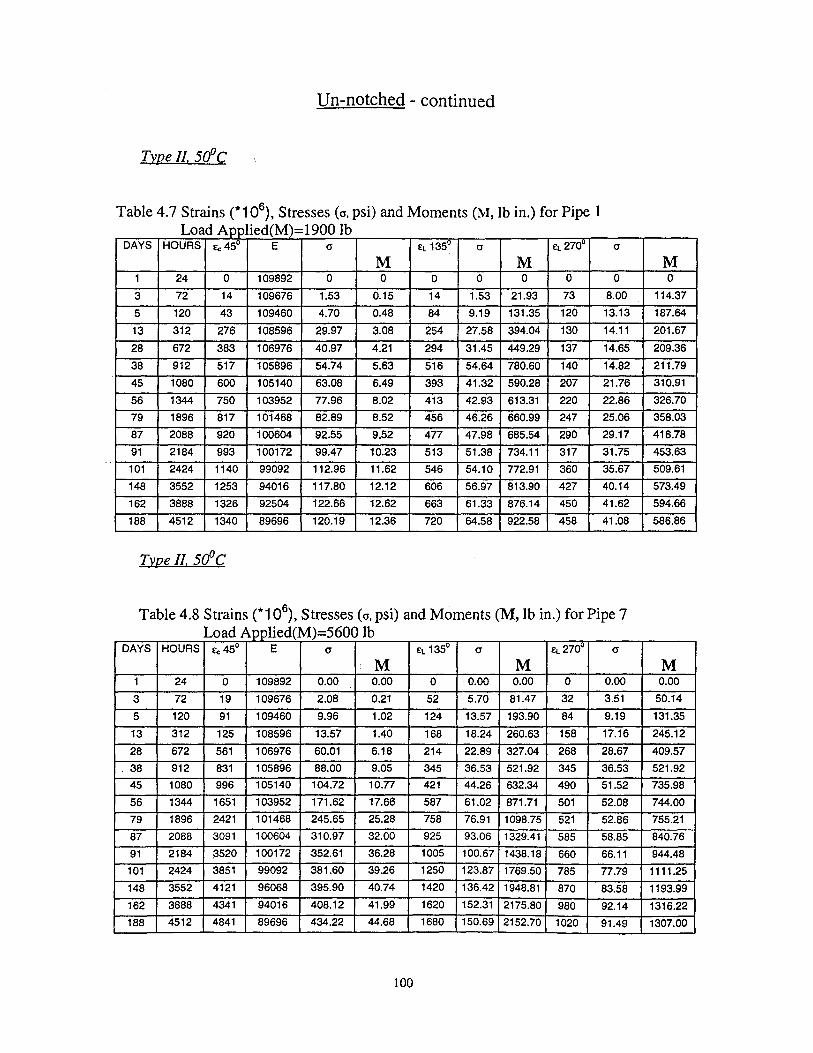
The effective stresses at the midsection were evaluated as follows:

The maximum stresses (from Table 4.4) were 436.82 and 192.73 psi for circumferential and longitudinal stresses, respectively. Therefore, the maximum effective stress was 379.17 psi, based on equation 4.5 (i.e. 7.5% deflection of the diameter), which is much less than 3000 psi (CPPA yield stress). The change of diameter is the governing factor and the CPPA limit is not reasonable for the general failure criterion of the buried HDPE pipe subjected to live loading.

101

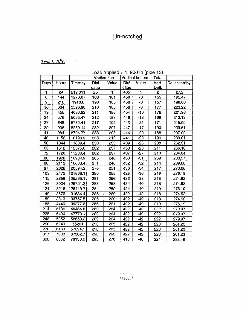
5.1.2. Evaluation of the long-term vertical change of diameter using Bi-

directional shifting method

The Bi-directional Shifting Function Method, Popelar et al. [1990]. It enables the

construction of master curves for nonpressurized HDPE sewer pipe material using creep

test data. In this procedure, no curve fitting is needed, which enables even a single data

point, representing any viscoelastic phenomenon determined at a given test temperature,

to be shifted to another temperature. Based on the time-temperature superposition

principle, the horizontal and vertical shift functions, aT and bT, respectively, are given

by:

aT = exp [-0.109 (T-Tr)]--------------------------------------- (5

.2) bT= exp [0.0116 (T-Tr)]--------------------------------------

(5.3)

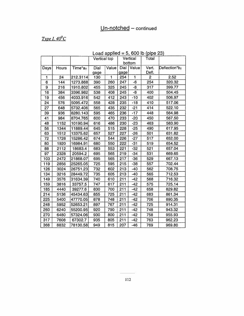
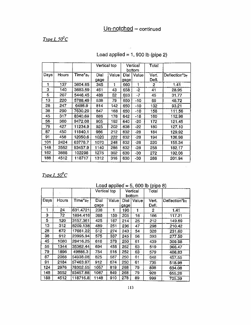
The master curves, based on the Bi-directional method are shown in Figs. 5.7 to

5.12. The data used for the Bi-directional plots are Appendix B.

117

APPENDIX B The values are for the Bi-directional method, which are shown in Figs. 5.7 to 5.12. Deflections (1/1000 in.)

118

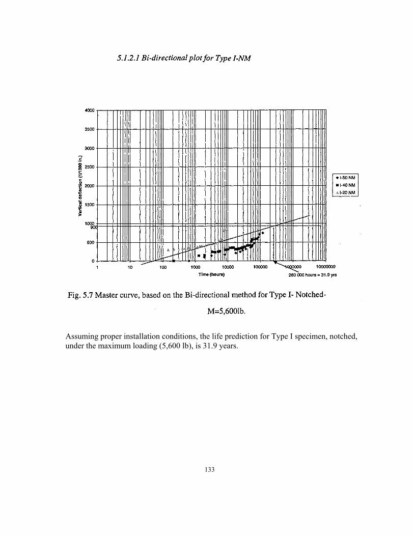
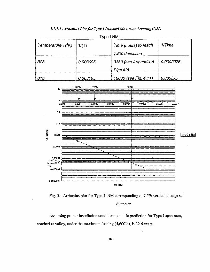
Assuming proper installation conditions, the life prediction for Type I specimen, notched, under the maximum loading (5,600 lb), is 31.9 years.

133

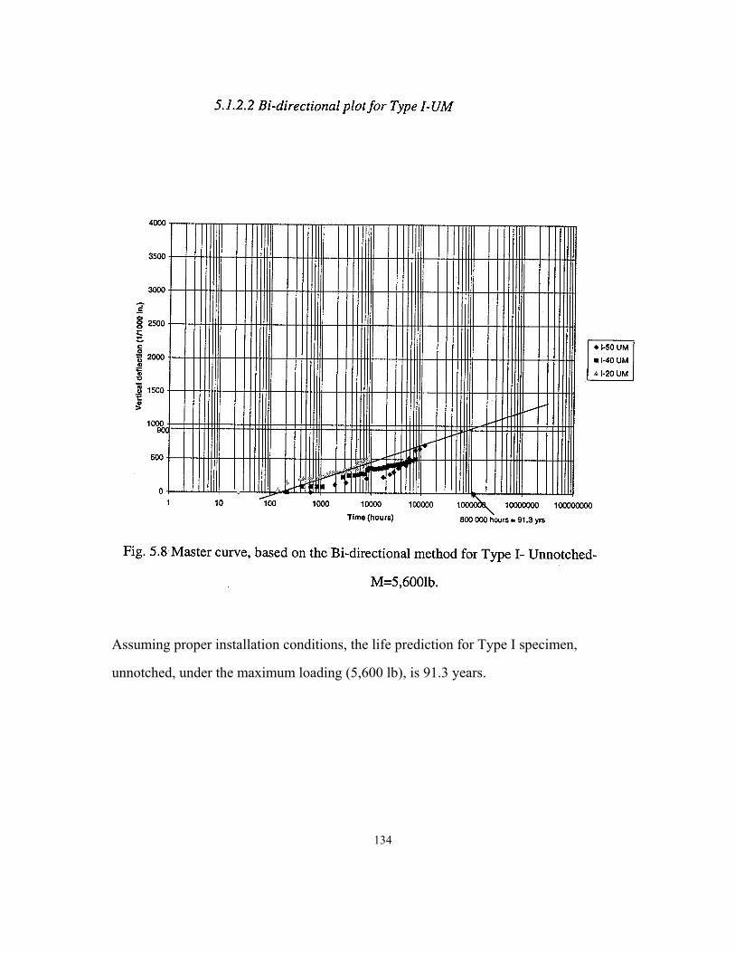
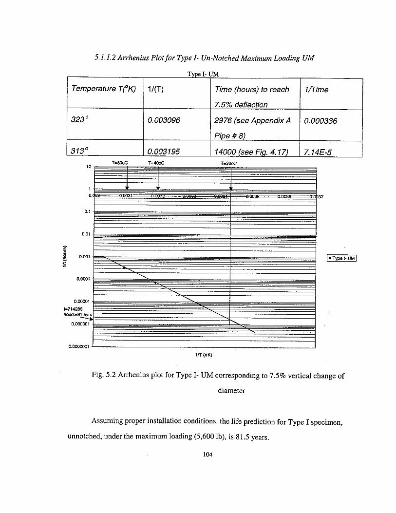
Assuming proper installation conditions, the life prediction for Type I specimen,

unnotched, under the maximum loading (5,600 lb), is 91.3 years.

134

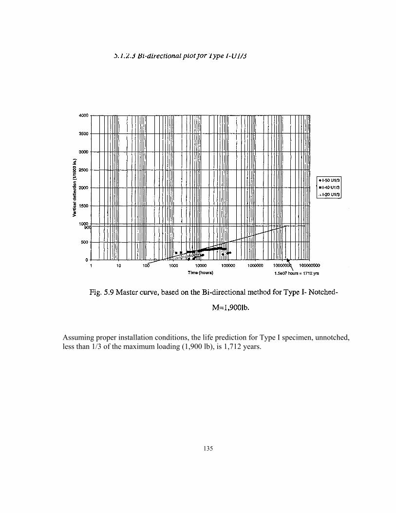
Assuming proper installation conditions, the life prediction for Type I specimen, unnotched, less than 1/3 of the maximum loading (1,900 lb), is 1,712 years.

135

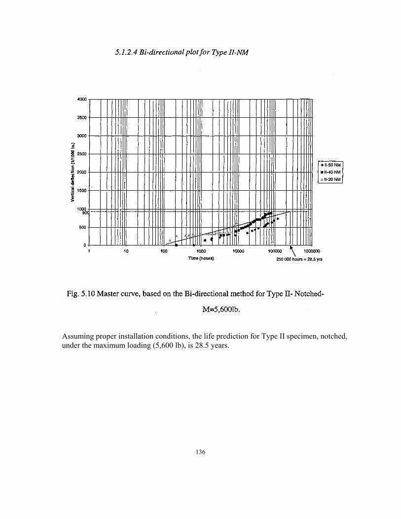
Assuming proper installation conditions, the life prediction for Type II specimen, notched, under the maximum loading (5,600 lb), is 28.5 years.

136

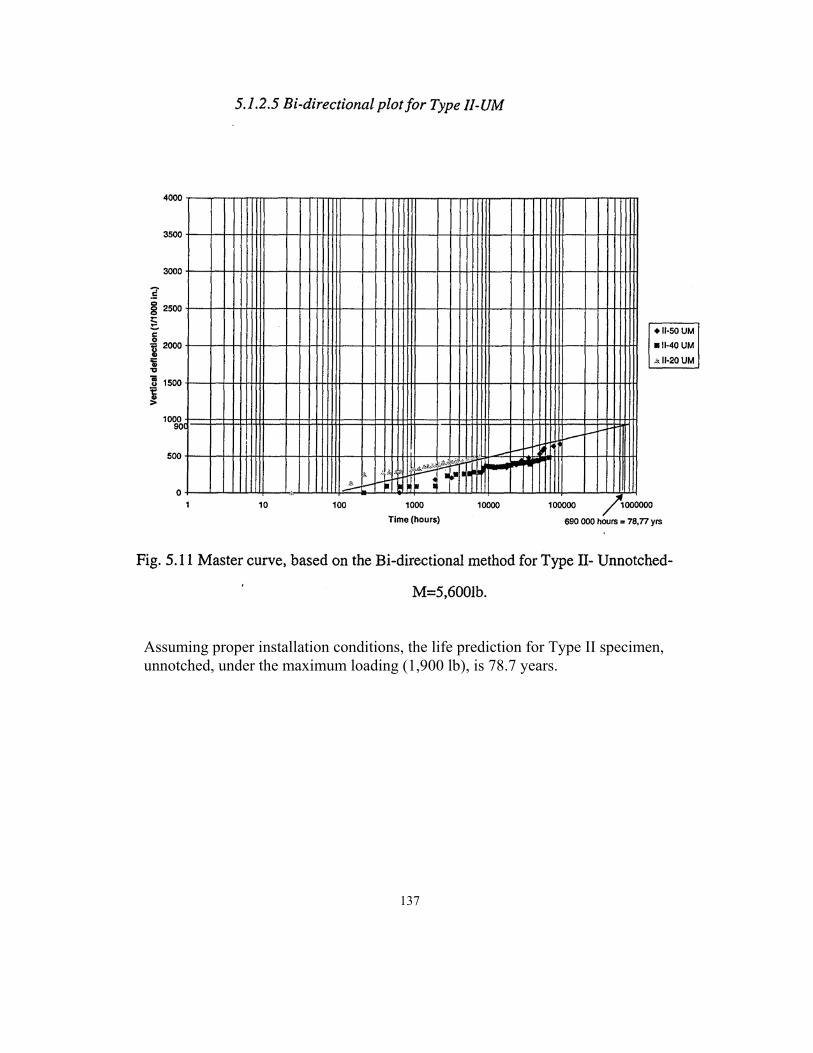
Assuming proper installation conditions, the life prediction for Type II specimen, unnotched, under the maximum loading (1,900 lb), is 78.7 years.

137

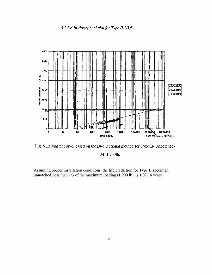
Assuming proper installation conditions, the life prediction for Type II specimen, unnotched, less than 1/3 of the maximum loading (1,900 lb), is 1,027.4 years.

138

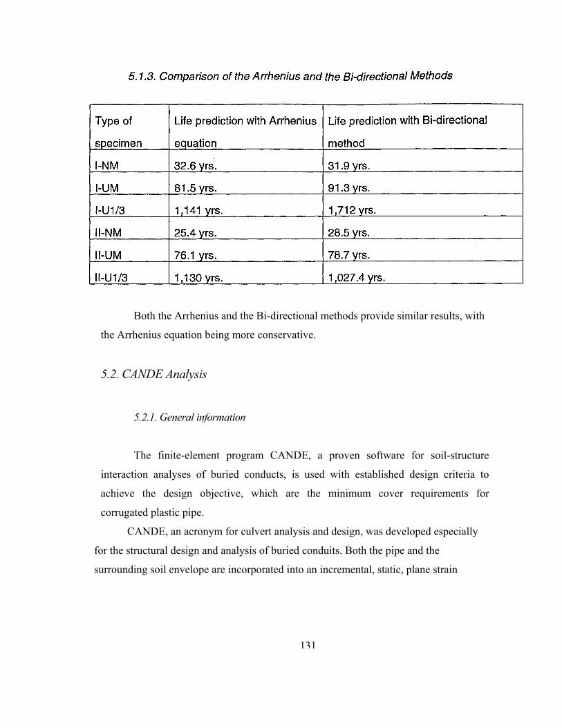
Both the Arrhenius and the Bi-directional methods provide similar results, with

the Arrhenius equation being more conservative.

5.2. CANDE Analysis

5.2.1. General information

The finite-element program CANDE, a proven software for soil-structure

interaction analyses of buried conducts, is used with established design criteria to

achieve the design objective, which are the minimum cover requirements for

corrugated plastic pipe.

CANDE, an acronym for culvert analysis and design, was developed especially

for the structural design and analysis of buried conduits. Both the pipe and the

surrounding soil envelope are incorporated into an incremental, static, plane strain

131

formulation. The pipe was modeled with a connected sequence of beam-column

elements, and the soil was modeled with continuum elements by using a revised linear

viscoelastic soil model. The fundamental analysis assumptions are small deformation

theory, linear elastic polyethylene properties (short-term) and a bonded pipe-soil

interface.

The gravity loading of the soil is applied in the first load step for the analysis of

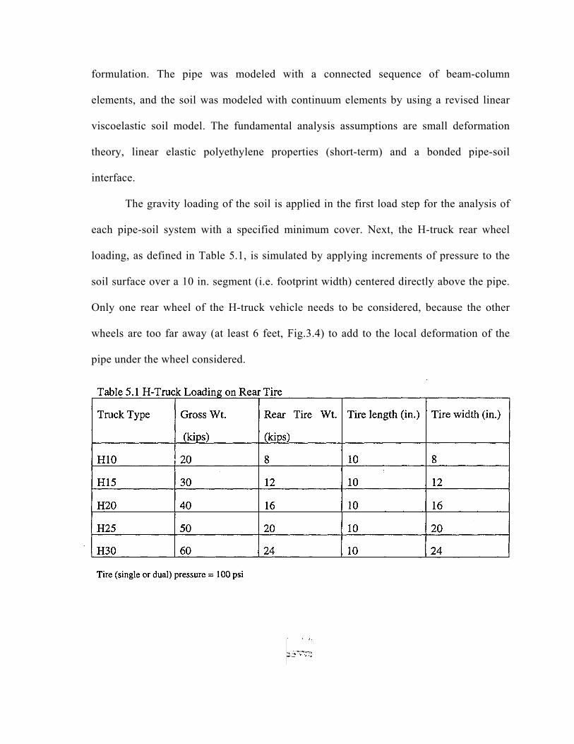
each pipe-soil system with a specified minimum cover. Next, the H-truck rear wheel

loading, as defined in Table 5.1, is simulated by applying increments of pressure to the

soil surface over a 10 in. segment (i.e. footprint width) centered directly above the pipe.

Only one rear wheel of the H-truck vehicle needs to be considered, because the other

wheels are too far away (at least 6 feet, Fig.3.4) to add to the local deformation of the

pipe under the wheel considered.

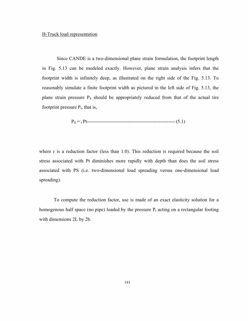
H-Truck load representation

Since CANDE is a two-dimensional plane strain formulation, the footprint length

in Fig. 5.13 can be modeled exactly. However, plane strain analysis infers that the

footprint width is infinitely deep, as illustrated on the right side of the Fig. 5.13. To

reasonably simulate a finite footprint width as pictured in the left side of Fig. 5.13, the

plane strain pressure PS should be appropriately reduced from that of the actual tire

footprint pressure Pt, that is,

PS = r Pt------------------------------------------------------ (5.1)

where r is a reduction factor (less than 1.0). This reduction is required because the soil

stress associated with Pt diminishes more rapidly with depth than does the soil stress

associated with PS (i.e. two-dimensional load spreading versus one-dimensional load

spreading).

To compute the reduction factor, use is made of an exact elasticity solution for a

homogenous half space (no pipe) loaded by the pressure Pt acting on a rectangular footing

with dimensions 2L by 2b.

141

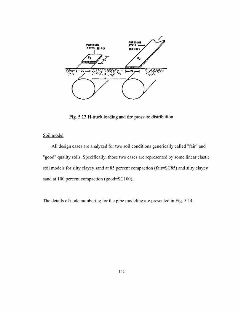
Soil model

All design cases are analyzed for two soil conditions generically called "fair" and

"good" quality soils. Specifically, those two cases are represented by some linear elastic

soil models for silty clayey sand at 85 percent compaction (fair=SC85) and silty clayey

sand at 100 percent compaction (good=SC100).

The details of node numbering for the pipe modeling are presented in Fig. 5.14.

142

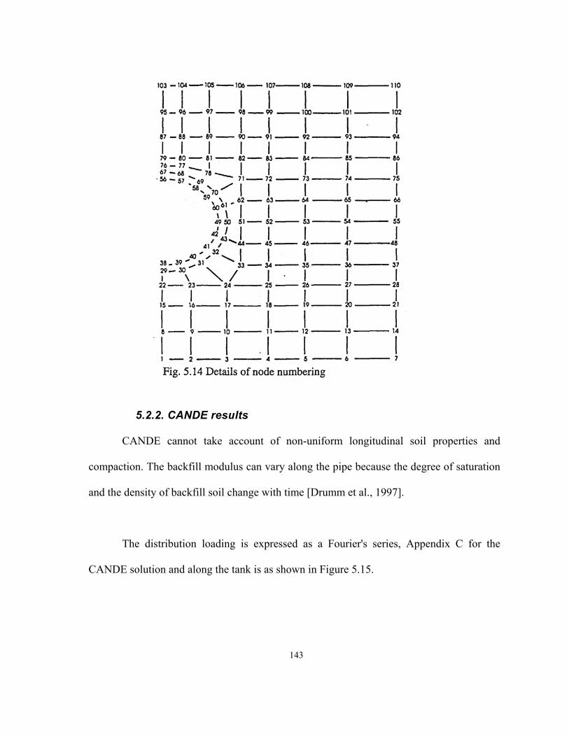
5.2.2. CANDE results

CANDE cannot take account of non-uniform longitudinal soil properties and

compaction. The backfill modulus can vary along the pipe because the degree of saturation

and the density of backfill soil change with time [Drumm et al., 1997].

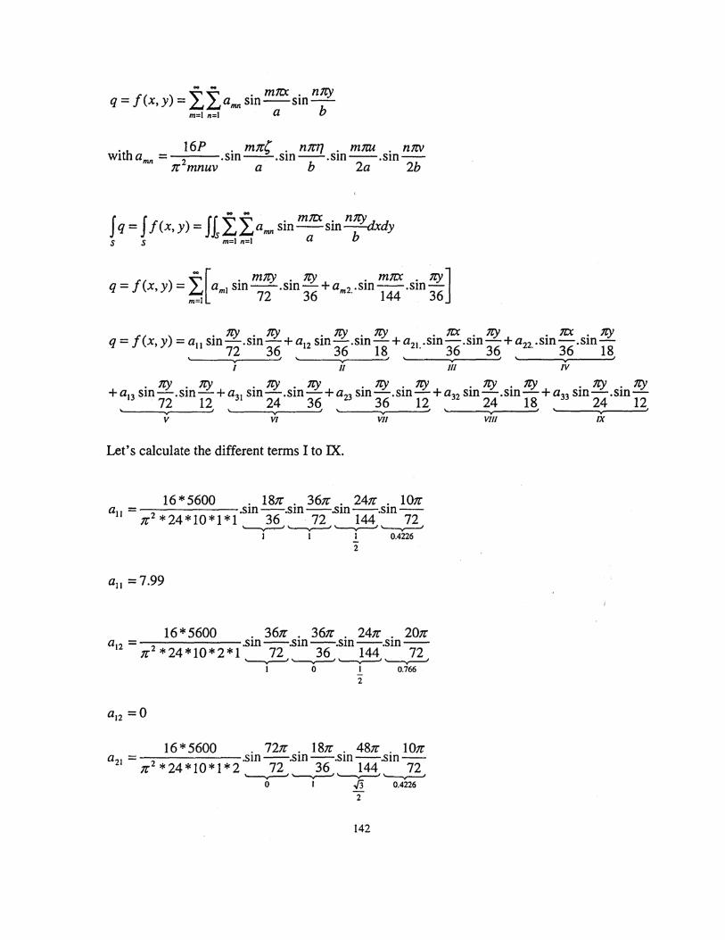
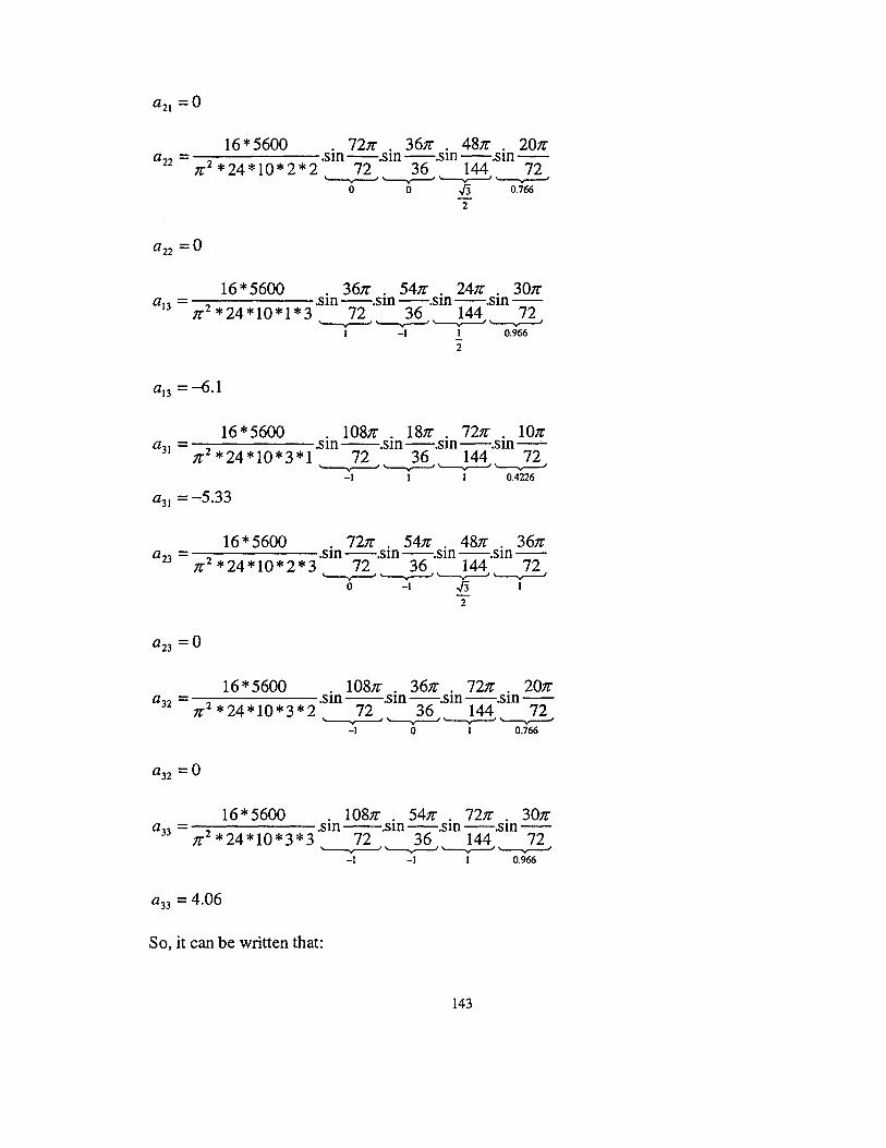
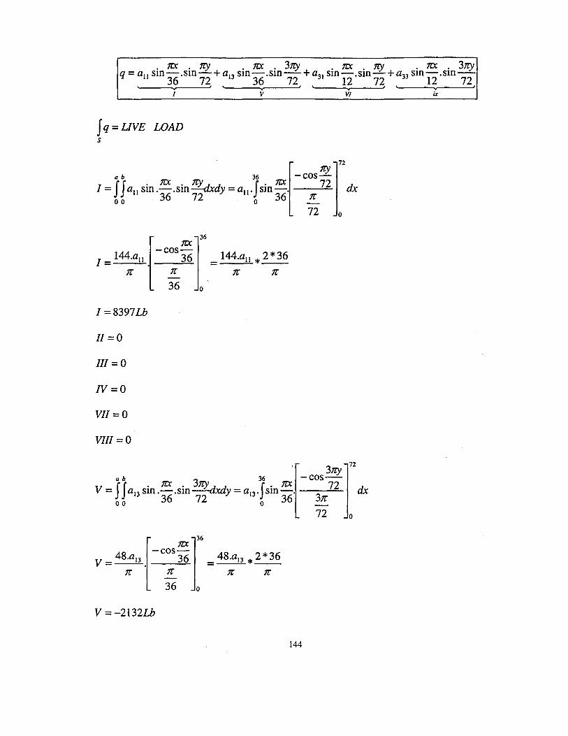
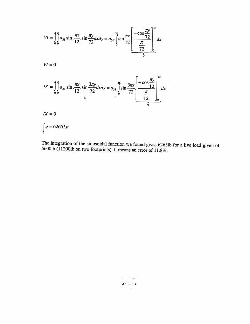
The distribution loading is expressed as a Fourier's series, Appendix C for the

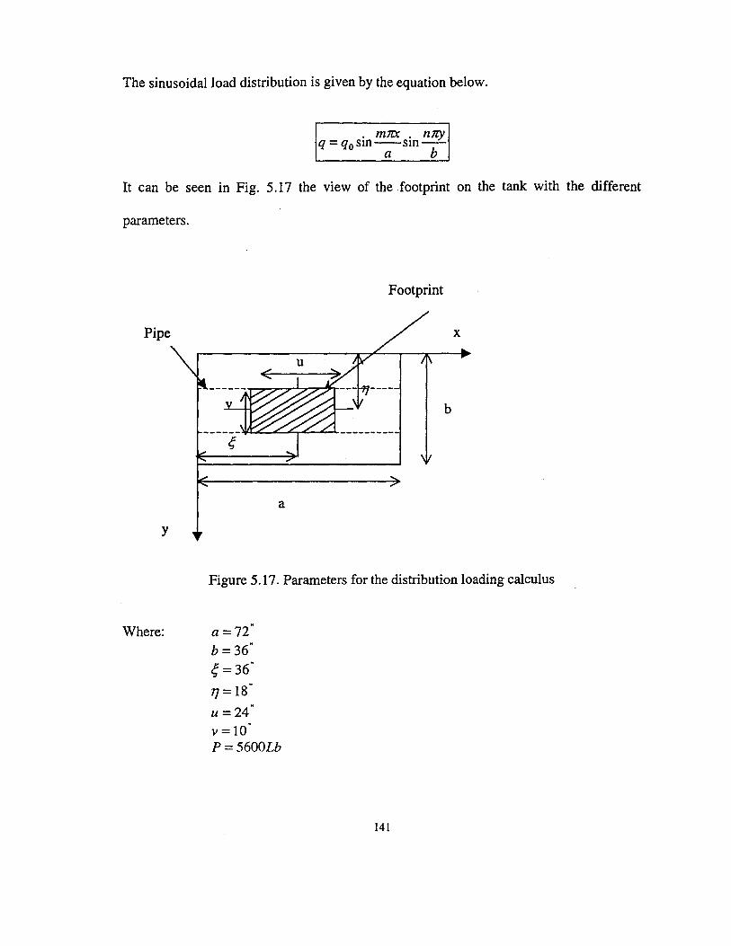
CANDE solution and along the tank is as shown in Figure 5.15.

143

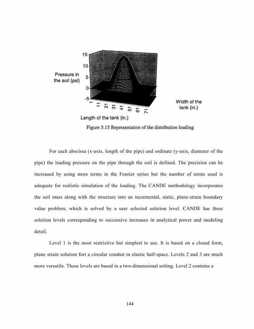
For each abscissa (x-axis, length of the pipe) and ordinate (y-axis, diameter of the

pipe) the loading pressure on the pipe through the soil is defined. The precision can be

increased by using more terms in the Fourier series but the number of terms used is

adequate for realistic simulation of the loading. The CANDE methodology incorporates

the soil mass along with the structure into an incremental, static, plane-strain boundary

value problem, which is solved by a user selected solution level. CANDE has three

solution levels corresponding to successive increases in analytical power and modeling

detail.

Level 1 is the most restrictive but simplest to use. It is based on a closed form,

plane strain solution fort a circular conduit in elastic half-space. Levels 2 and 3 are much

more versatile. These levels are based in a two-dimensional setting. Level 2 contains a

144

completely automated mesh generation routine suitable for most of the typical

culvert installations and pipe shapes. Included are generators for circular, elliptical,

rectangular and arch geometry. Thus, no special knowledge of finite element mesh is

required by user for this level. Level 3, which is applicable to arbitrary soil-structure

configurations such as non-symmetric installations and miscellaneous shapes, can

provide a more general solution than the other levels. However, it requires the user

to have knowledge of finite techniques in order to prepare and input the mesh

topology of the soil-structure system. The solution level concept permits the user to

choose the degree of rigor and effort commensurate with the worth of a particular

project and the confidence in the system input variables. For a designer, this means

CANDE is not only available to perform a quick, approximate design for input into a

feasibility study. It can also be used as a rigorous analytical tool in the detail design

phase. For the analyst, it offers extended flexibility in performing parametric studies

and comparative research.

One of the main problems in the use of this software is that CANDE 89 is

twodimensional software. In this way, we cannot get the deflections along the length

of the pipe directly. CANDE 89 gives the deflection of a ring of the pipe at a given

abscissa. Typically if a pipe is 80 inches long, CANDE89 needs to be run at 80

successive longitudinal locations at one inch spacing to get a realistic deflected

profile.

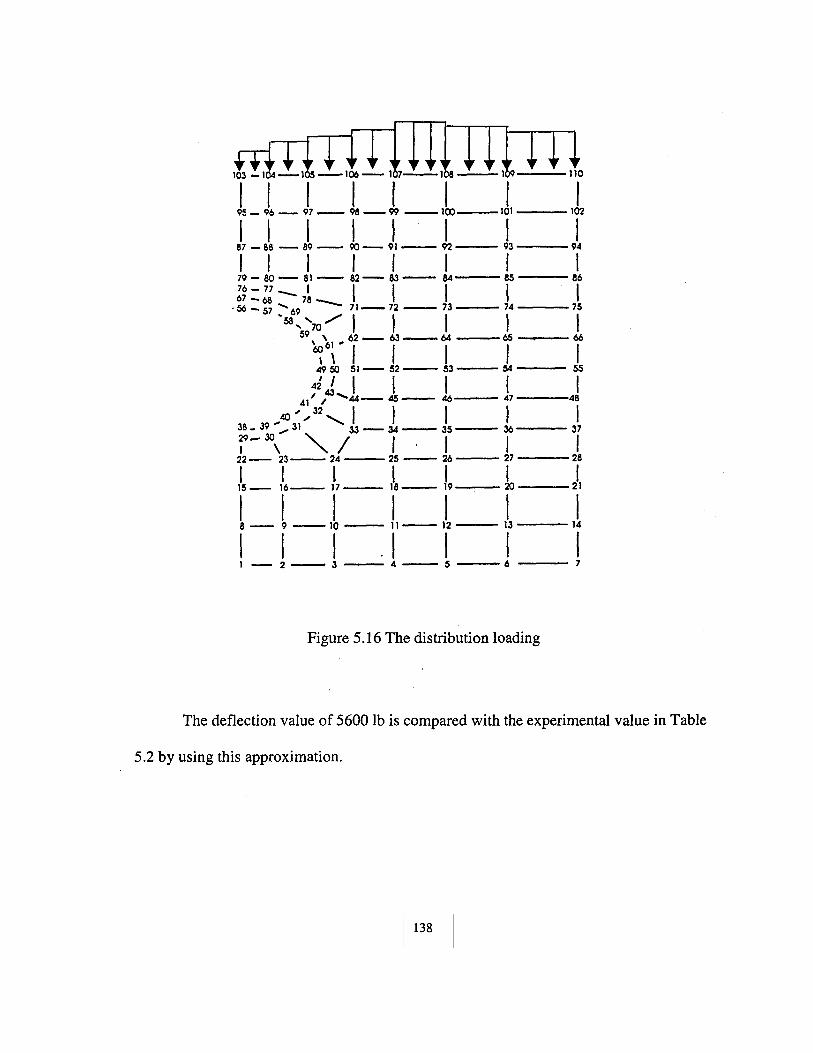
Finally in CANDE 89, the loading is selected across the cross-section for a

given abscissa above the soil on the nodes from 103 to 110 as shown in Fig.5.16. A

uniform loading is defined for each element by taking the averages for the CANDE

89 input.

137

APPENDIX CFourier Simulation of Loading

140

CHAPTER 6

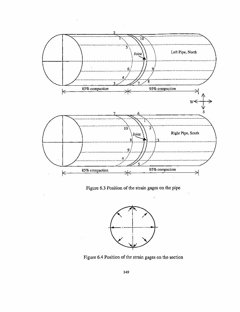
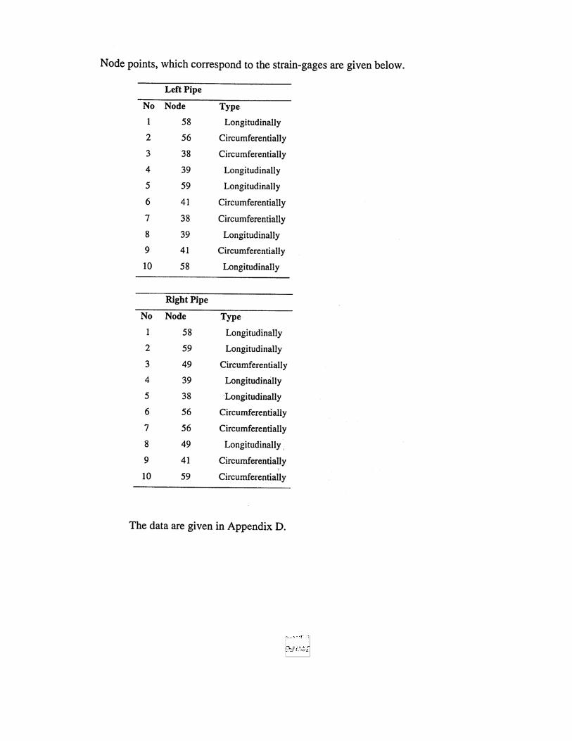
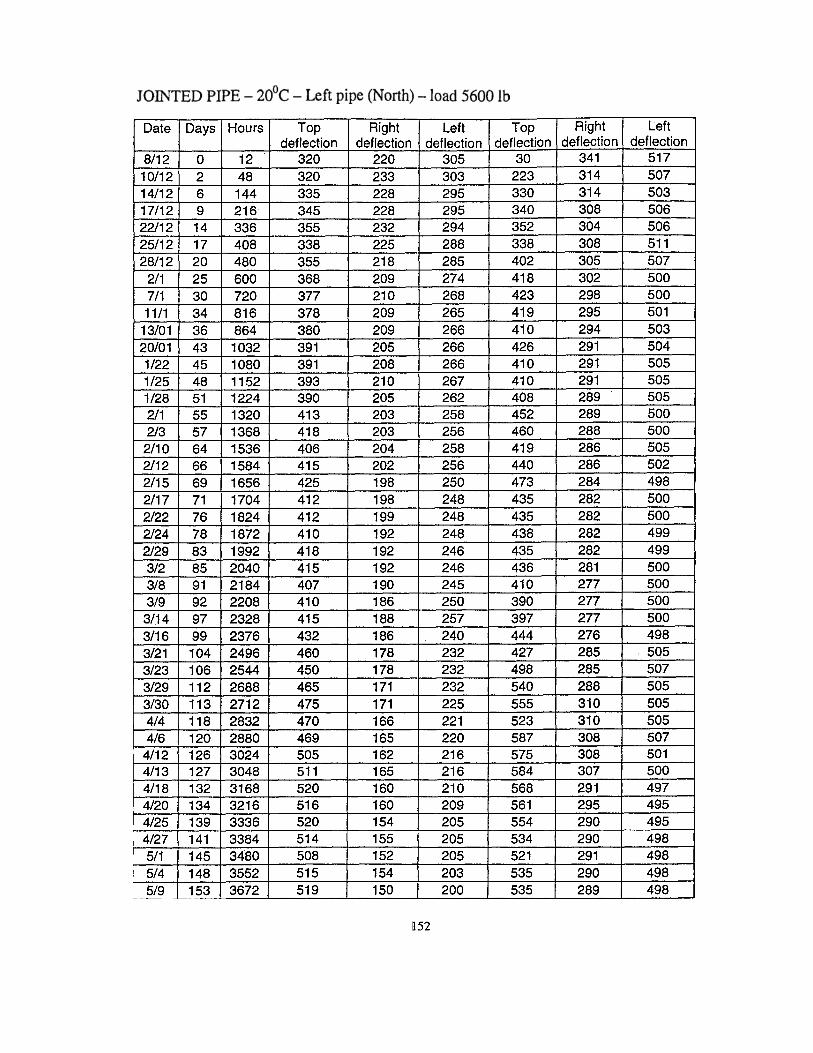
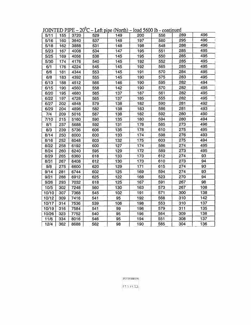
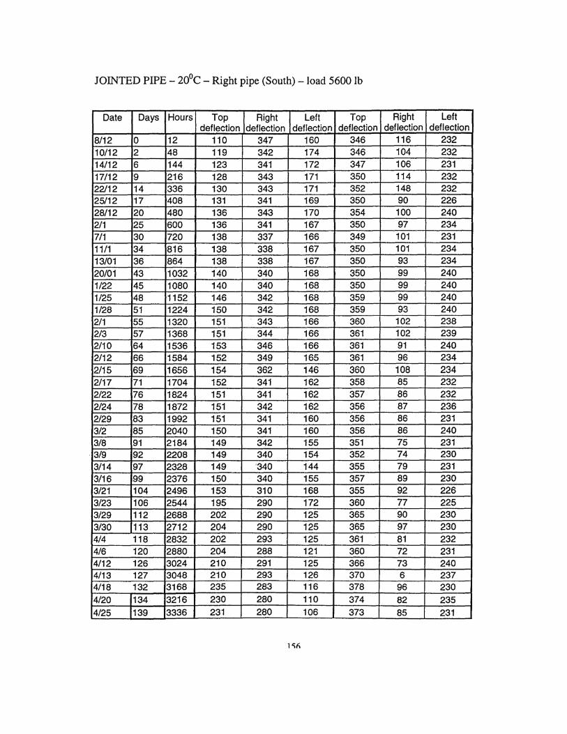
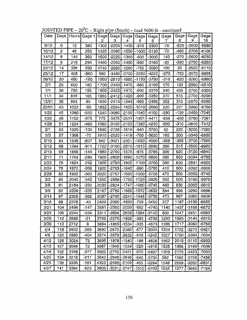
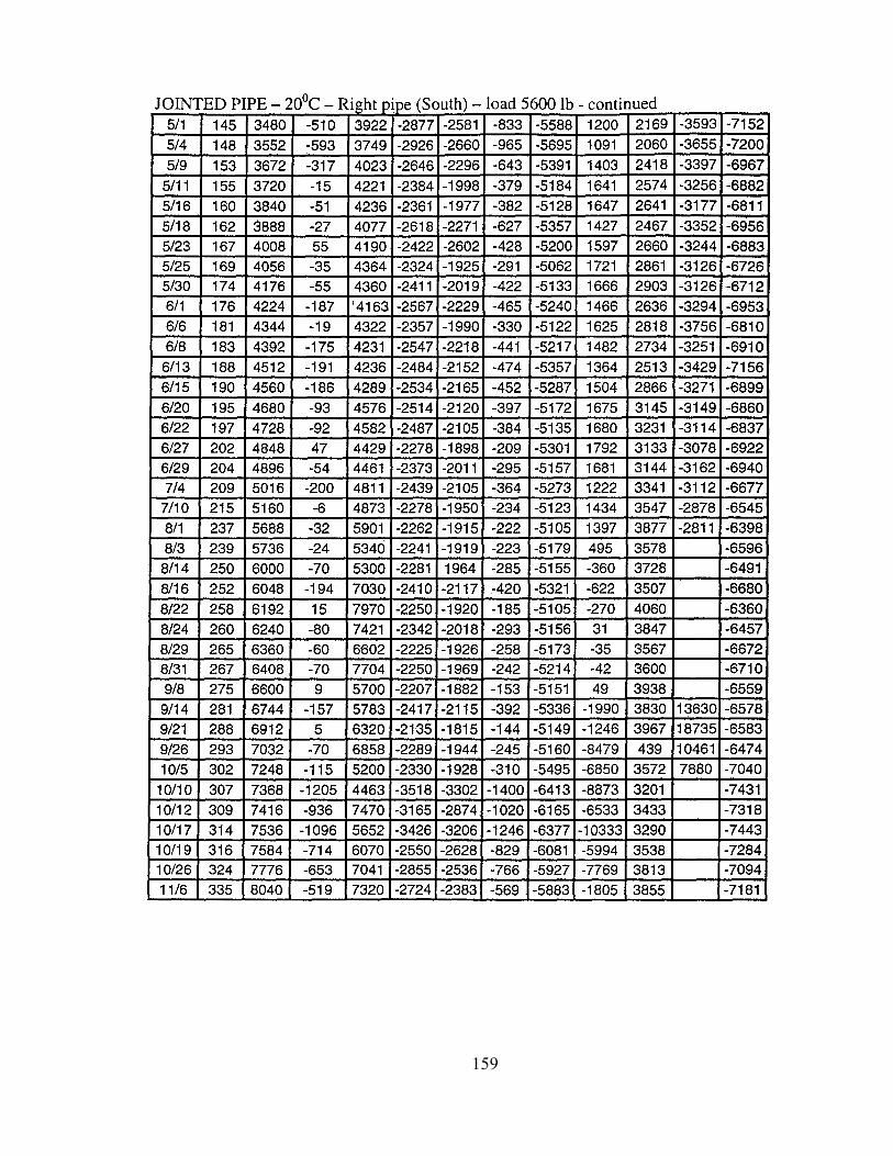
INVESTIGATION of JOINTED PIPE

In this chapter, jointed pipes were investigated both experimentally and

numerically to determine the deflection, stress and bending moment values. The pipes

used in the experiment and the mounted dial gages are shown in Figs. 6.1 and 6.2, and the

strain gages in Figs. 6.3 and 6.4.

153

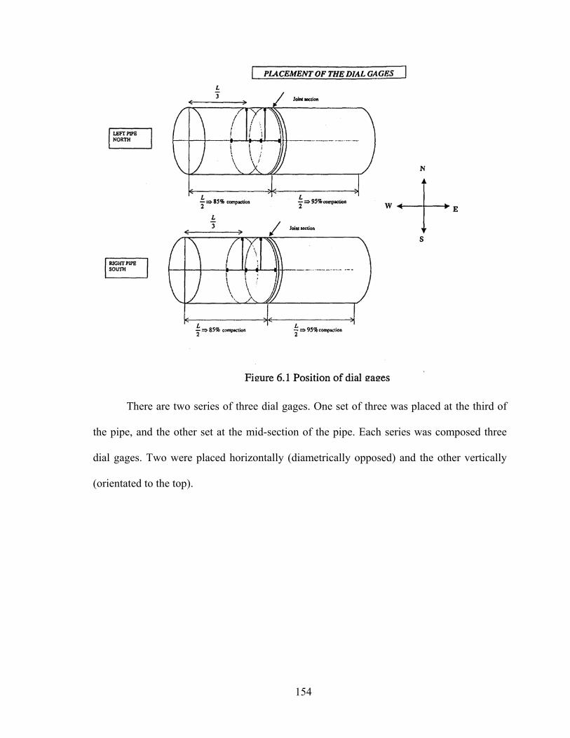
There are two series of three dial gages. One set of three was placed at the third of

the pipe, and the other set at the mid-section of the pipe. Each series was composed three

dial gages. Two were placed horizontally (diametrically opposed) and the other vertically

(orientated to the top).

154

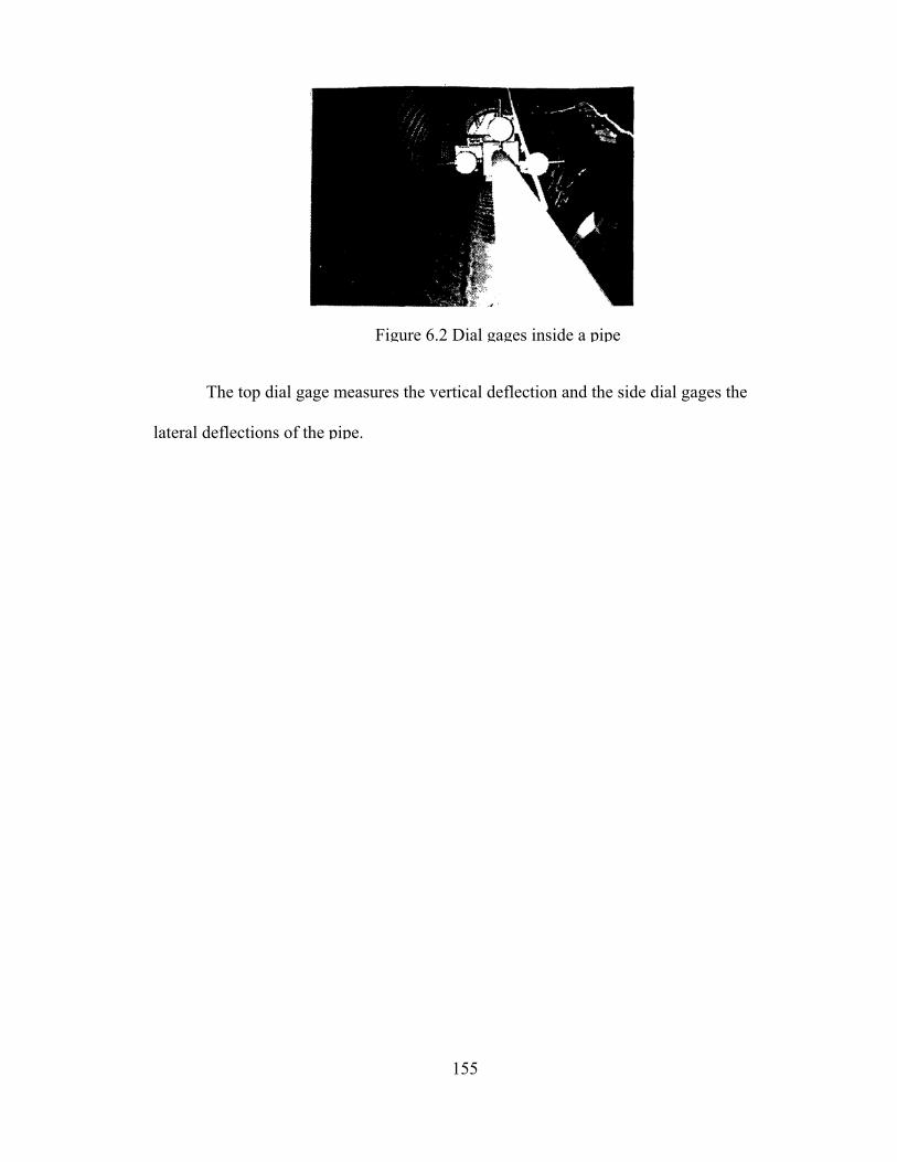
Figure 6.2 Dial gages inside a pipe

The top dial gage measures the vertical deflection and the side dial gages the

lateral deflections of the pipe.

155

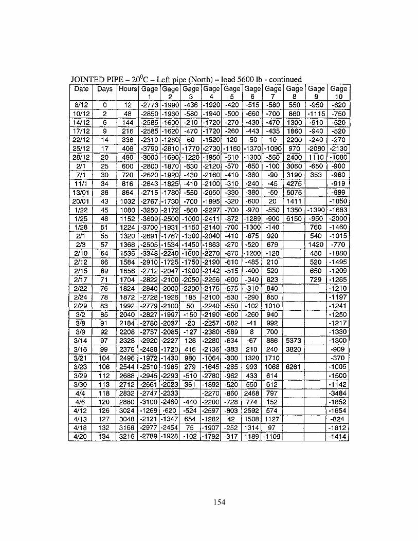
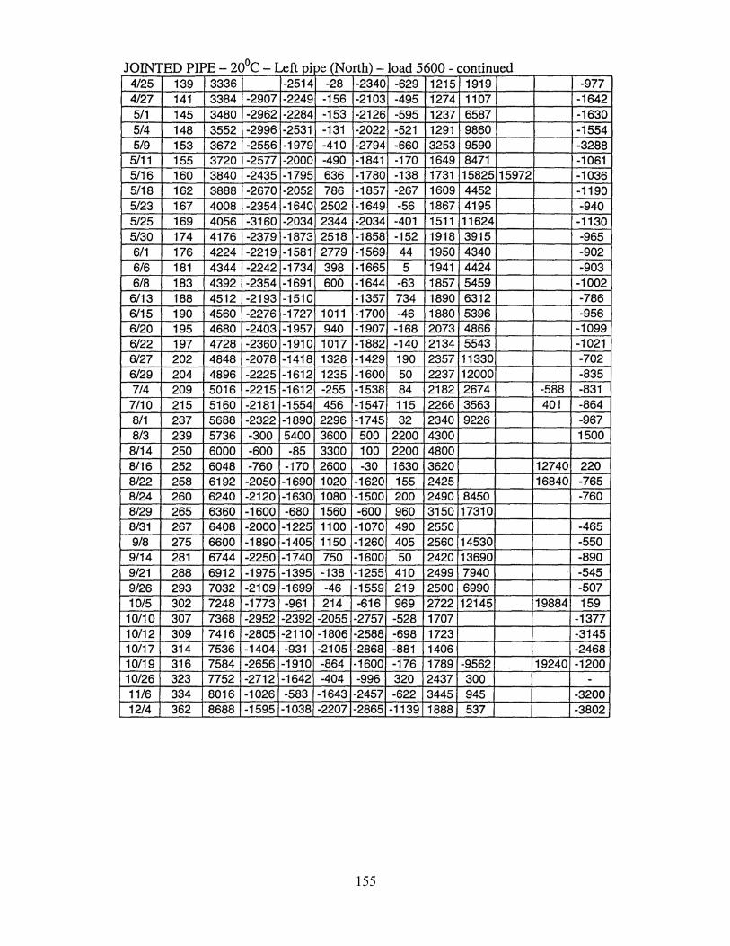
APPENDIX D Deflection and strain values for jointed pipe

Deflections(1/1000in.)

151

154

155

157

158

159

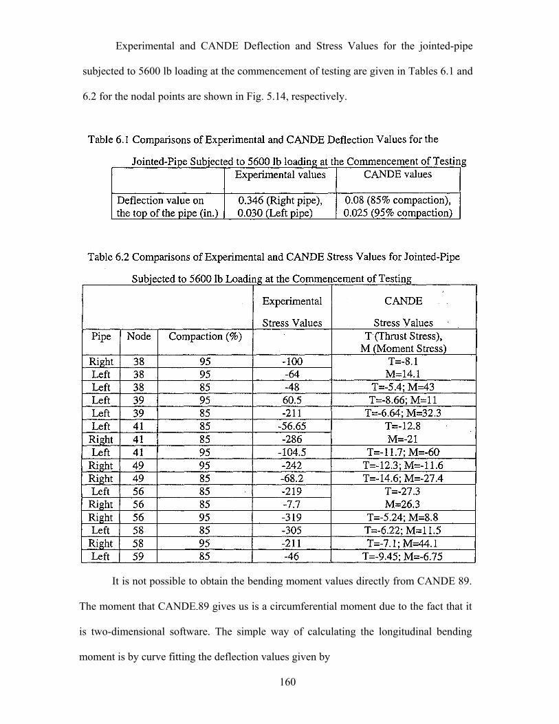
Experimental and CANDE Deflection and Stress Values for the jointed-pipe

subjected to 5600 lb loading at the commencement of testing are given in Tables 6.1 and

6.2 for the nodal points are shown in Fig. 5.14, respectively.

It is not possible to obtain the bending moment values directly from CANDE 89.

The moment that CANDE-89 gives us is a circumferential moment due to the fact that it

is two-dimensional software. The simple way of calculating the longitudinal bending

moment is by curve fitting the deflection values given by

160

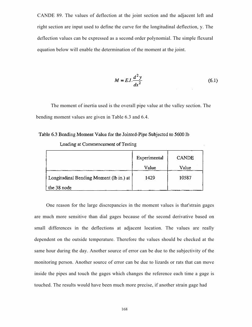
CANDE 89. The values of deflection at the joint section and the adjacent left and

right section are input used to define the curve for the longitudinal deflection, y. The

deflection values can be expressed as a second order polynomial. The simple flexural

equation below will enable the determination of the moment at the joint.

The moment of inertia used is the overall pipe value at the valley section. The

bending moment values are given in Table 6.3 and 6.4.

One reason for the large discrepancies in the moment values is that'strain gages

are much more sensitive than dial gages because of the second derivative based on

small differences in the deflections at adjacent location. The values are really

dependent on the outside temperature. Therefore the values should be checked at the

same hour during the day. Another source of error can be due to the subjectivity of the

monitoring person. Another source of error can be due to lizards or rats that can move

inside the pipes and touch the gages which changes the reference each time a gage is

touched. The results would have been much more precise, if another strain gage had

168

been placed on the outer diameter at each location. The stresses on the both sides

of the pipe wall would enable the separation of the thrust and bending effects.

The principal purpose of these experiments and analytical studies were to

verify if the joint was adequate to avoid leakage. As the two compactions of the

sand interface at the joint, the shear stress is max at this location. Experimental

study shows 143.22 and -646.8psi, at gage 2 and 10 in the south pipe at the

commencement of testing, respectively. But these values reach 702.72 and -690psi

during the experiment. Internal pressure of 74.5kPa(10.8psi) for initiation of

leakage in the type of coupler with O-ring corresponds 707psi axial stress (ASTM

D3212). It seems to be the governing failure criterion.

169

CHAPTER 7

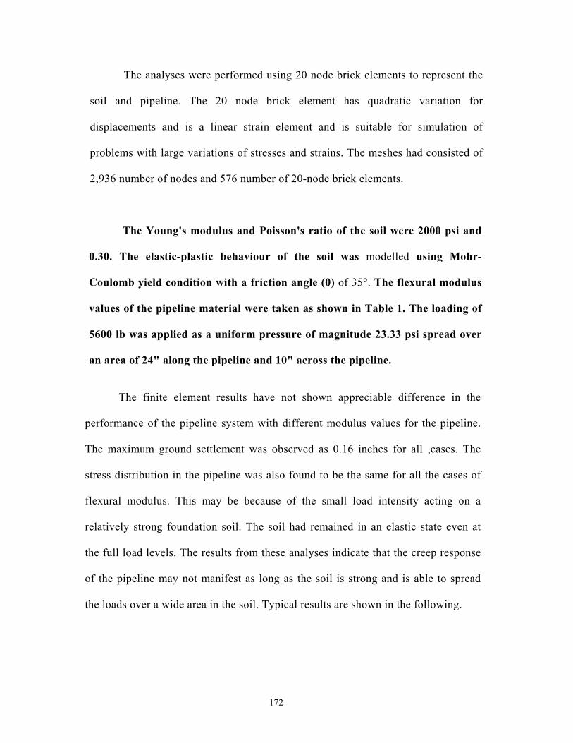
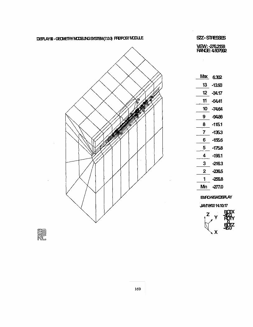
THREE DIMENSIONAL FINITE ELEMENT ANALYSIS OF INTERACTION BETWEEN HDPE PIPELINE AND SOIL

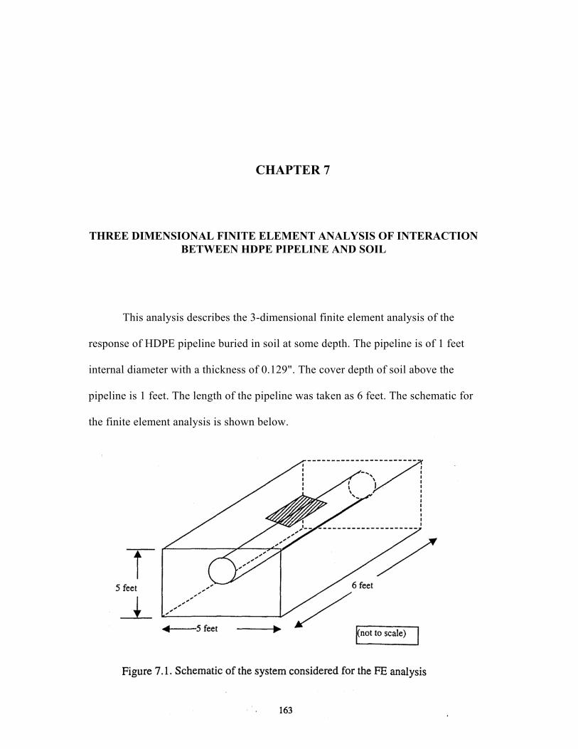
This analysis describes the 3-dimensional finite element analysis of the

response of HDPE pipeline buried in soil at some depth. The pipeline is of 1 feet

internal diameter with a thickness of 0.129". The cover depth of soil above the

pipeline is 1 feet. The length of the pipeline was taken as 6 feet. The schematic for

the finite element analysis is shown below.

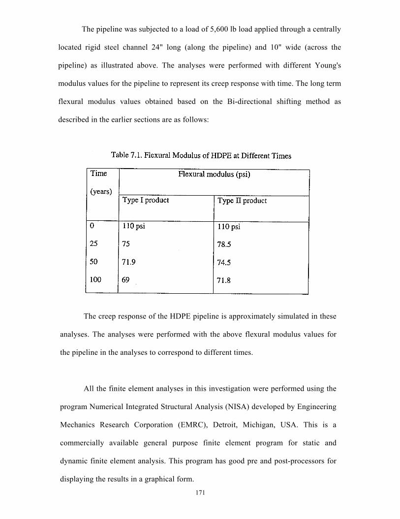
The pipeline was subjected to a load of 5,600 lb load applied through a centrally

located rigid steel channel 24" long (along the pipeline) and 10" wide (across the

pipeline) as illustrated above. The analyses were performed with different Young's

modulus values for the pipeline to represent its creep response with time. The long term

flexural modulus values obtained based on the Bi-directional shifting method as

described in the earlier sections are as follows:

The creep response of the HDPE pipeline is approximately simulated in these

analyses. The analyses were performed with the above flexural modulus values for

the pipeline in the analyses to correspond to different times.

All the finite element analyses in this investigation were performed using the

program Numerical Integrated Structural Analysis (NISA) developed by Engineering

Mechanics Research Corporation (EMRC), Detroit, Michigan, USA. This is a

commercially available general purpose finite element program for static and

dynamic finite element analysis. This program has good pre and post-processors for

displaying the results in a graphical form.

171

The analyses were performed using 20 node brick elements to represent the

soil and pipeline. The 20 node brick element has quadratic variation for

displacements and is a linear strain element and is suitable for simulation of

problems with large variations of stresses and strains. The meshes had consisted of

2,936 number of nodes and 576 number of 20-node brick elements.

The Young's modulus and Poisson's ratio of the soil were 2000 psi and

0.30. The elastic-plastic behaviour of the soil was modelled using Mohr-

Coulomb yield condition with a friction angle (0) of 35°. The flexural modulus

values of the pipeline material were taken as shown in Table 1. The loading of

5600 lb was applied as a uniform pressure of magnitude 23.33 psi spread over

an area of 24" along the pipeline and 10" across the pipeline.

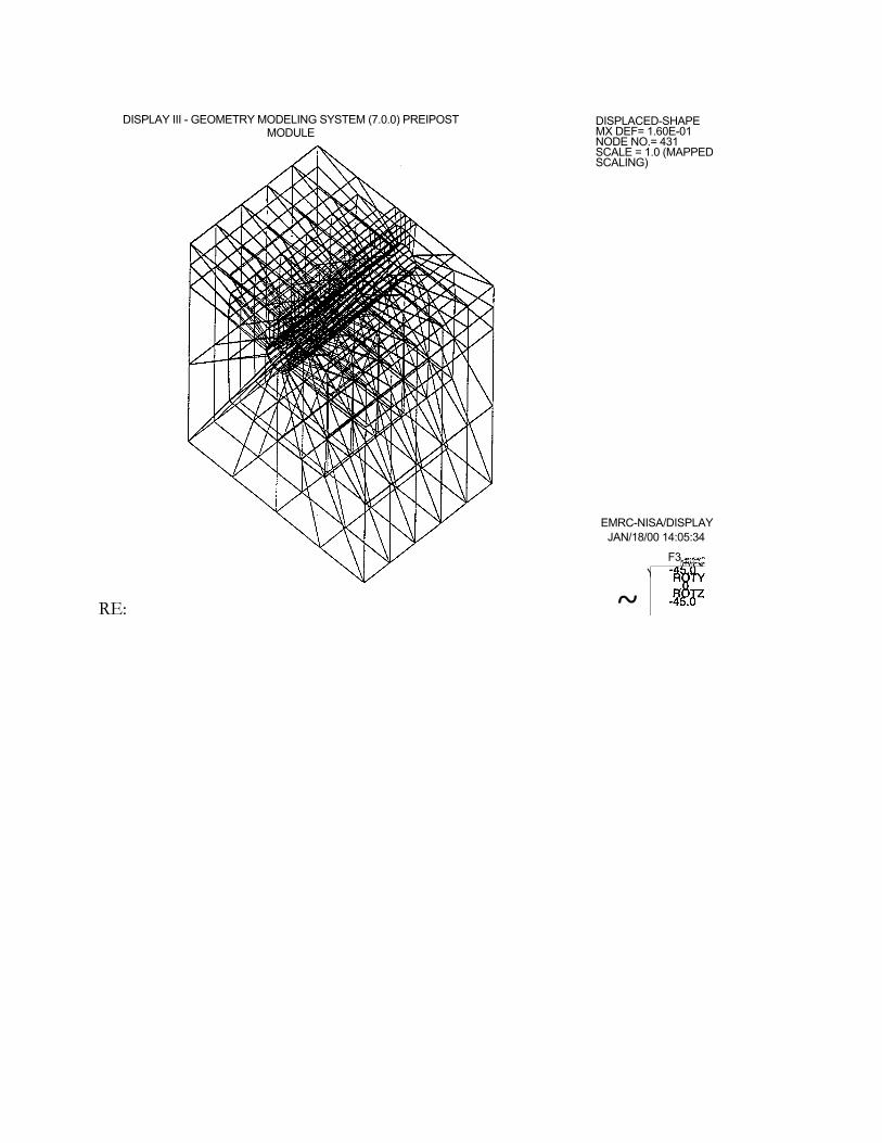
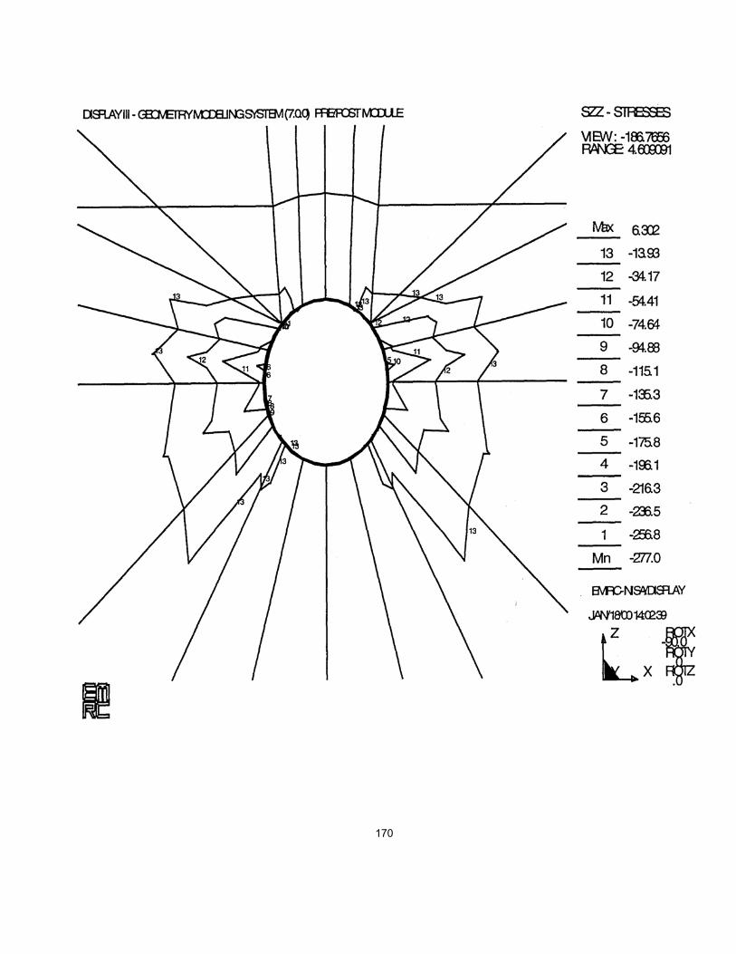
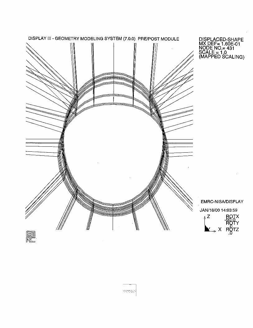
The finite element results have not shown appreciable difference in the

performance of the pipeline system with different modulus values for the pipeline.

The maximum ground settlement was observed as 0.16 inches for all ,cases. The

stress distribution in the pipeline was also found to be the same for all the cases of

flexural modulus. This may be because of the small load intensity acting on a

relatively strong foundation soil. The soil had remained in an elastic state even at

the full load levels. The results from these analyses indicate that the creep response

of the pipeline may not manifest as long as the soil is strong and is able to spread

the loads over a wide area in the soil. Typical results are shown in the following.

172

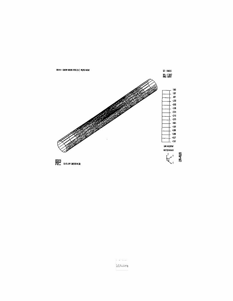
DISPLAY III - GEOMETRY MODELING SYSTEM (7.0.0) PREIPOST MODULE

DISPLACED-SHAPE MX DEF= 1.60E-01 NODE NO.= 431 SCALE = 1.0 (MAPPED SCALING)

EMRC-NISA/DISPLAY JAN/18/00 14:05:34

F3 Y

~ RE:

170

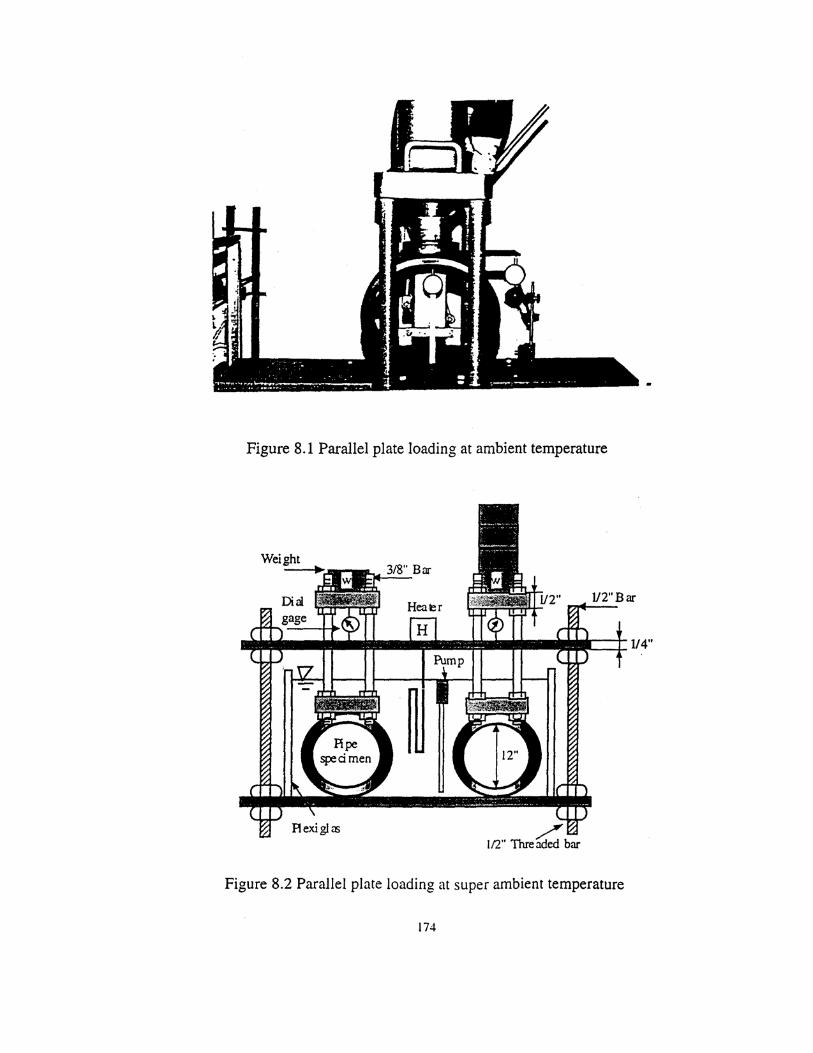
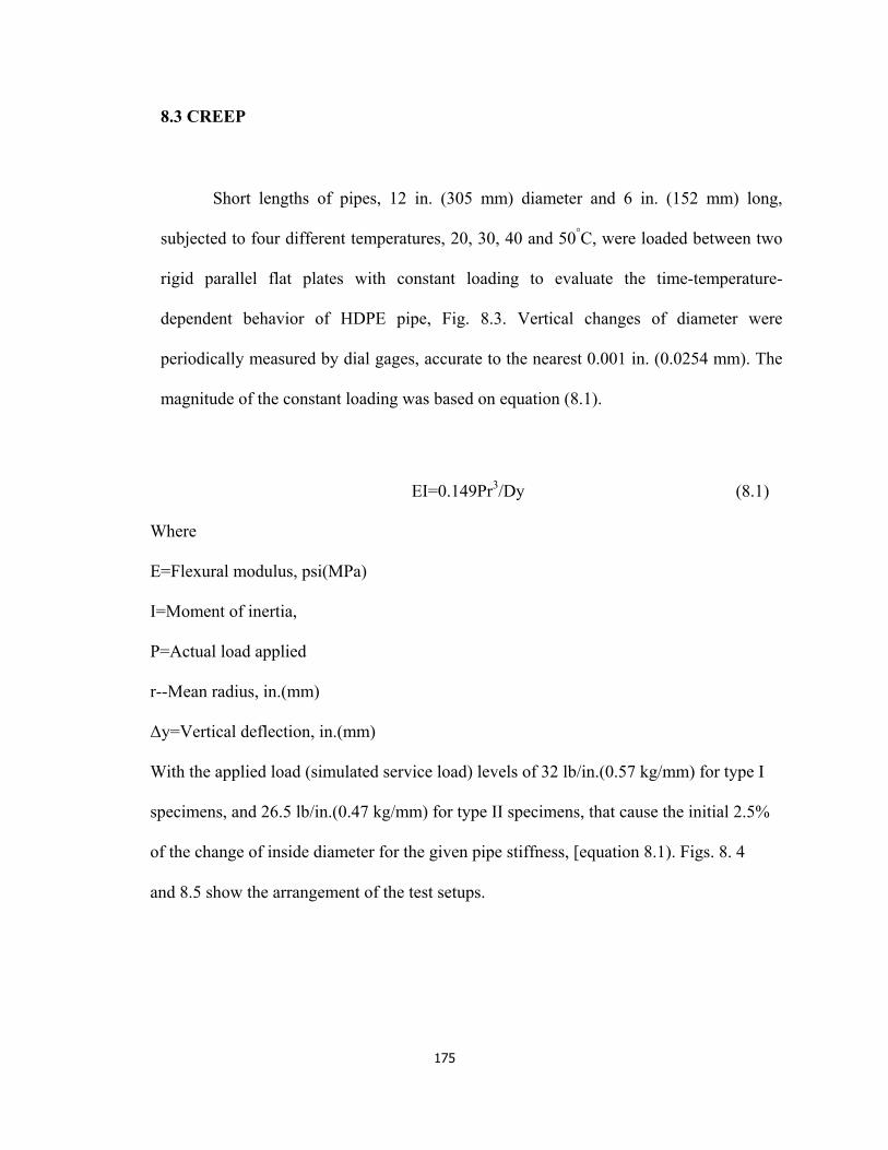
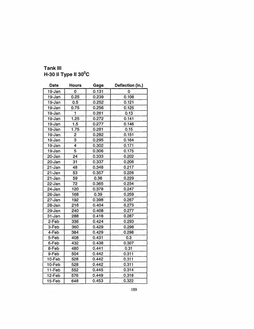
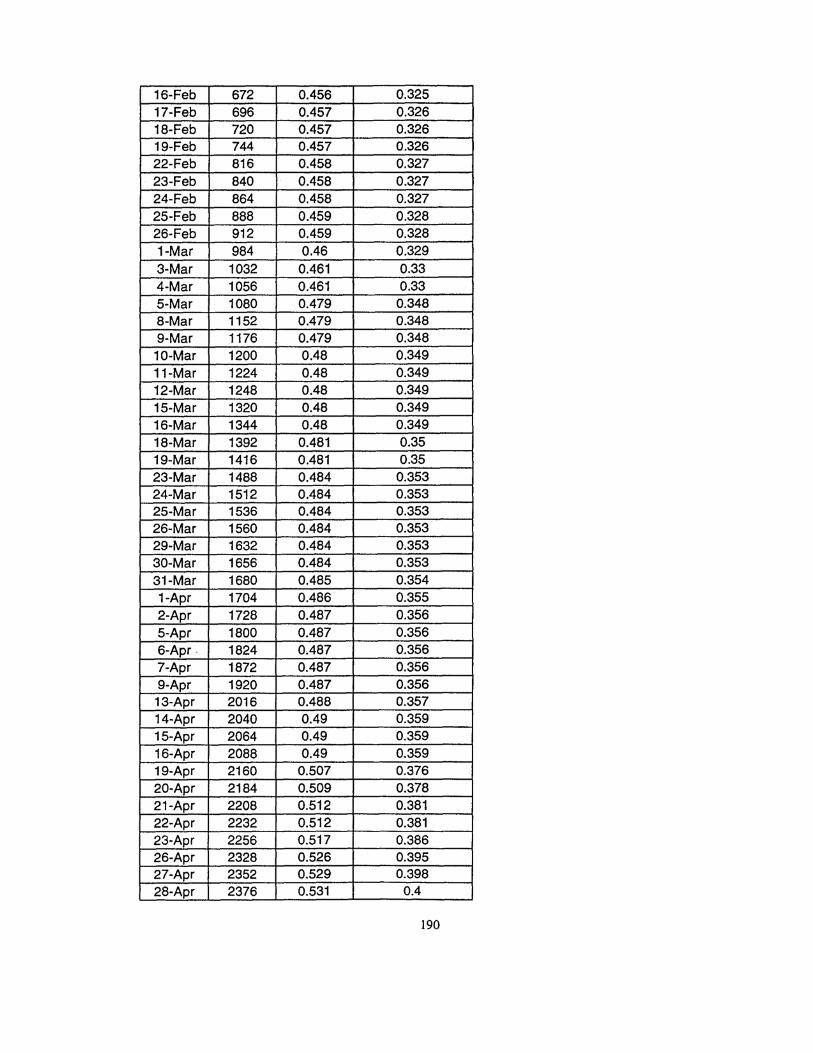
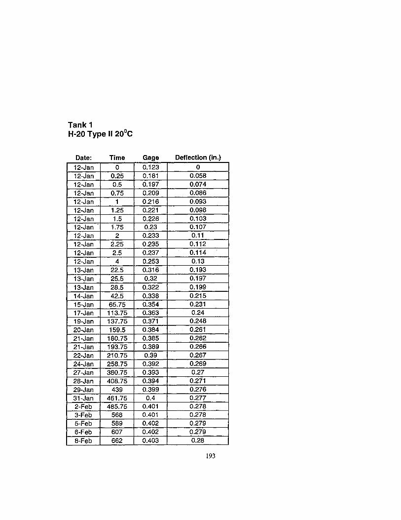
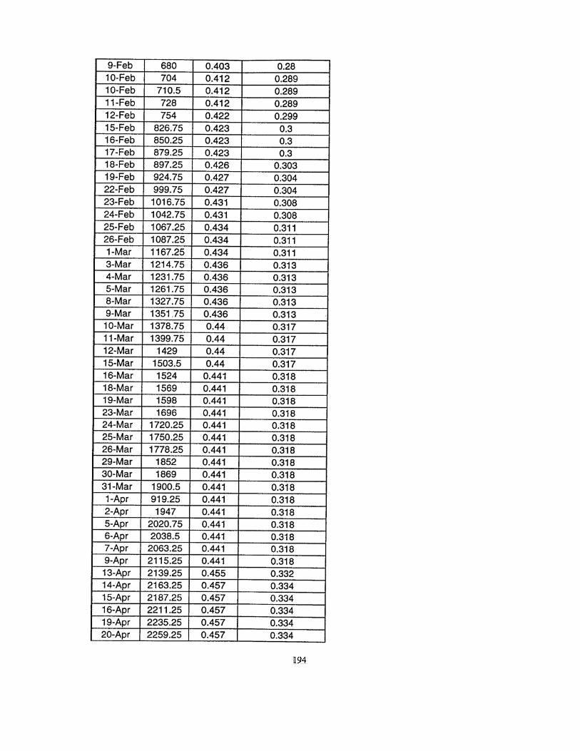
8.3 CREEP

Short lengths of pipes, 12 in. (305 mm) diameter and 6 in. (152 mm) long,

subjected to four different temperatures, 20, 30, 40 and 50°C, were loaded between two

rigid parallel flat plates with constant loading to evaluate the time-temperature-

dependent behavior of HDPE pipe, Fig. 8.3. Vertical changes of diameter were

periodically measured by dial gages, accurate to the nearest 0.001 in. (0.0254 mm). The

magnitude of the constant loading was based on equation (8.1).

EI=0.149Pr3/Dy (8.1)

Where

E=Flexural modulus, psi(MPa)

I=Moment of inertia,

P=Actual load applied

r--Mean radius, in.(mm)

∆y=Vertical deflection, in.(mm)

With the applied load (simulated service load) levels of 32 lb/in.(0.57 kg/mm) for type I

specimens, and 26.5 lb/in.(0.47 kg/mm) for type II specimens, that cause the initial 2.5%

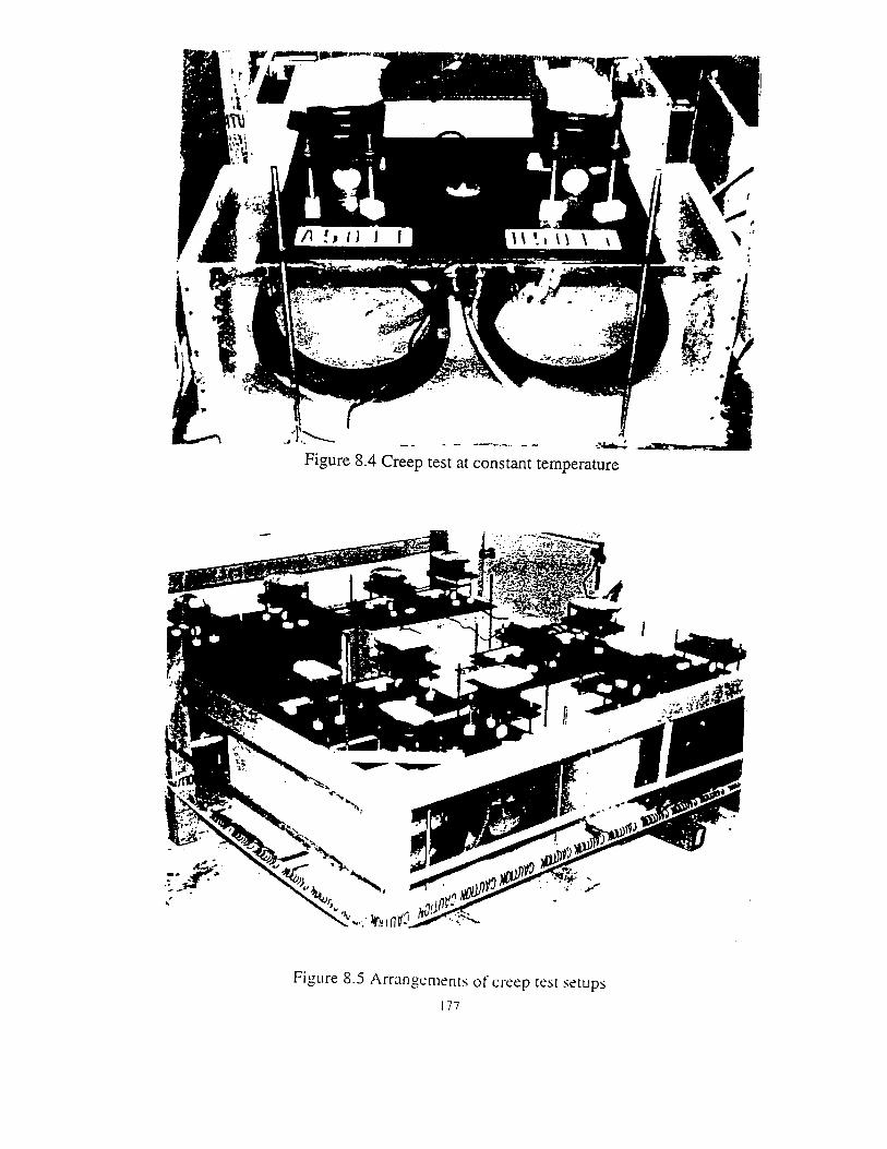
of the change of inside diameter for the given pipe stiffness, [equation 8.1). Figs. 8. 4

and 8.5 show the arrangement of the test setups.

175

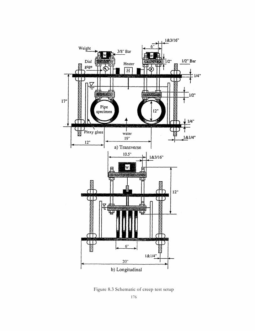
Figure 8.3 Schematic of creep test setup 176

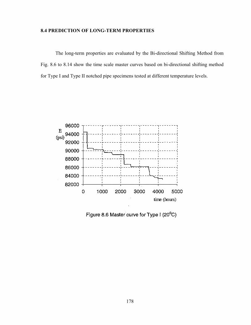
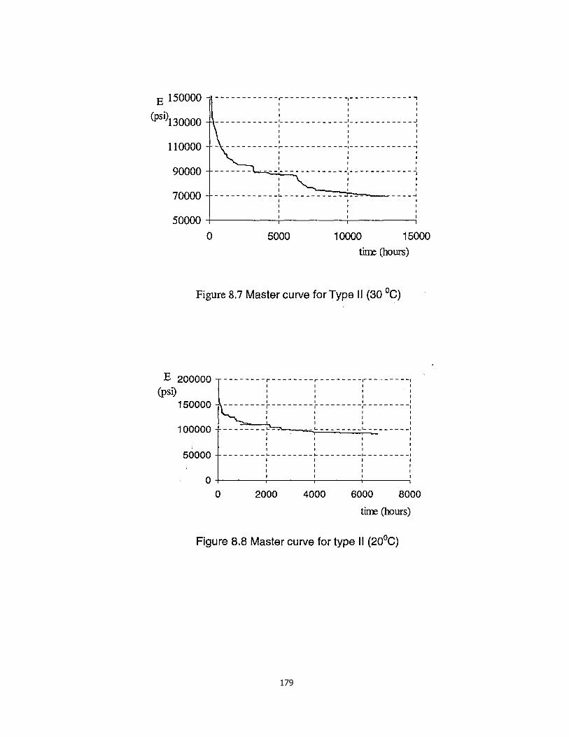
8.4 PREDICTION OF LONG-TERM PROPERTIES

The long-term properties are evaluated by the Bi-directional Shifting Method from

Fig. 8.6 to 8.14 show the time scale master curves based on bi-directional shifting method

for Type I and Type II notched pipe specimens tested at different temperature levels.

178

179

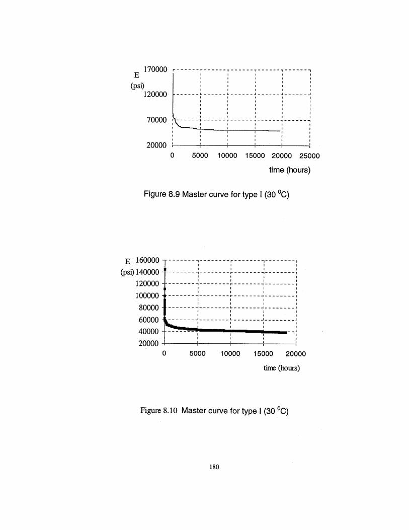
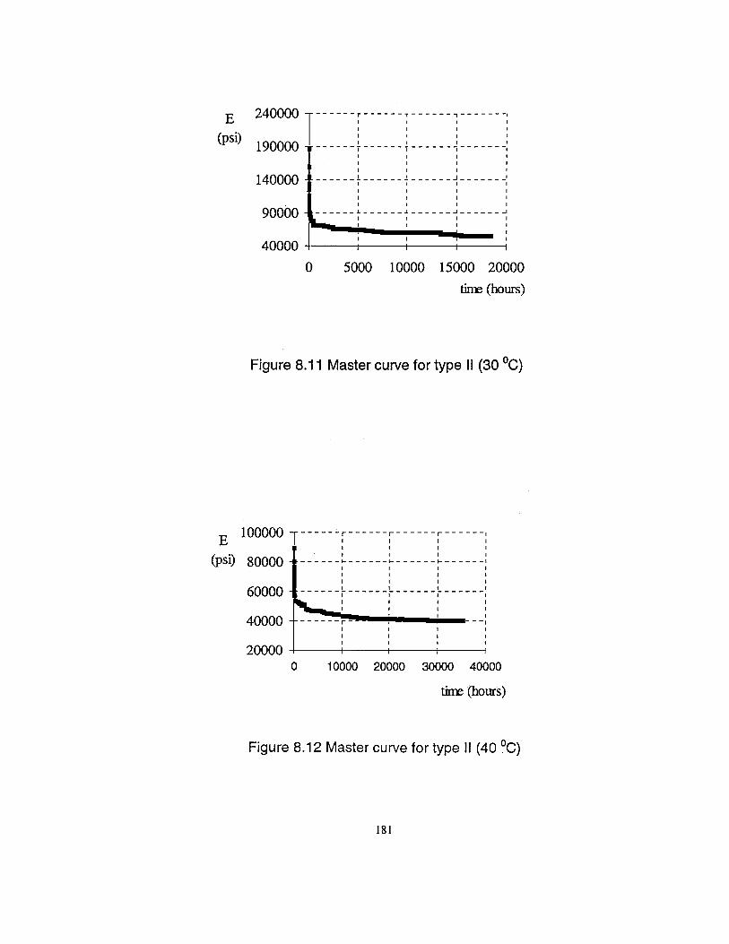
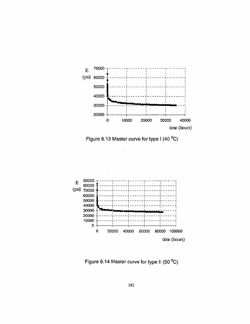
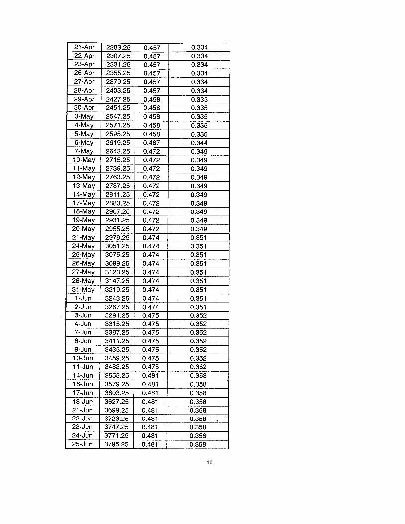
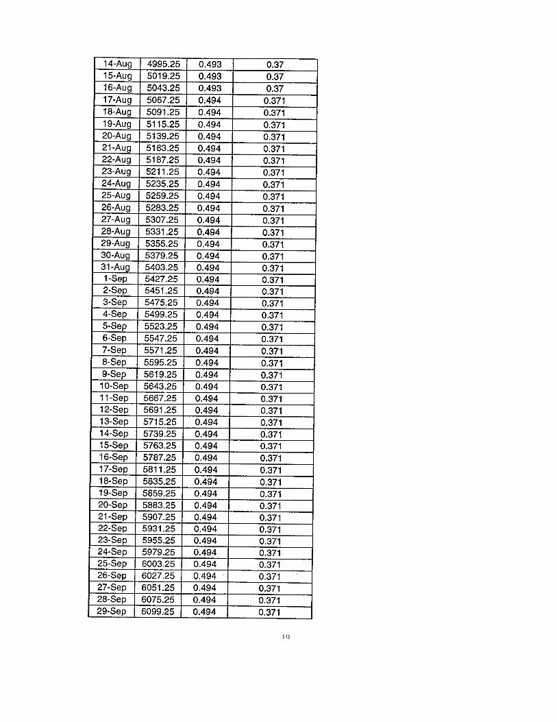
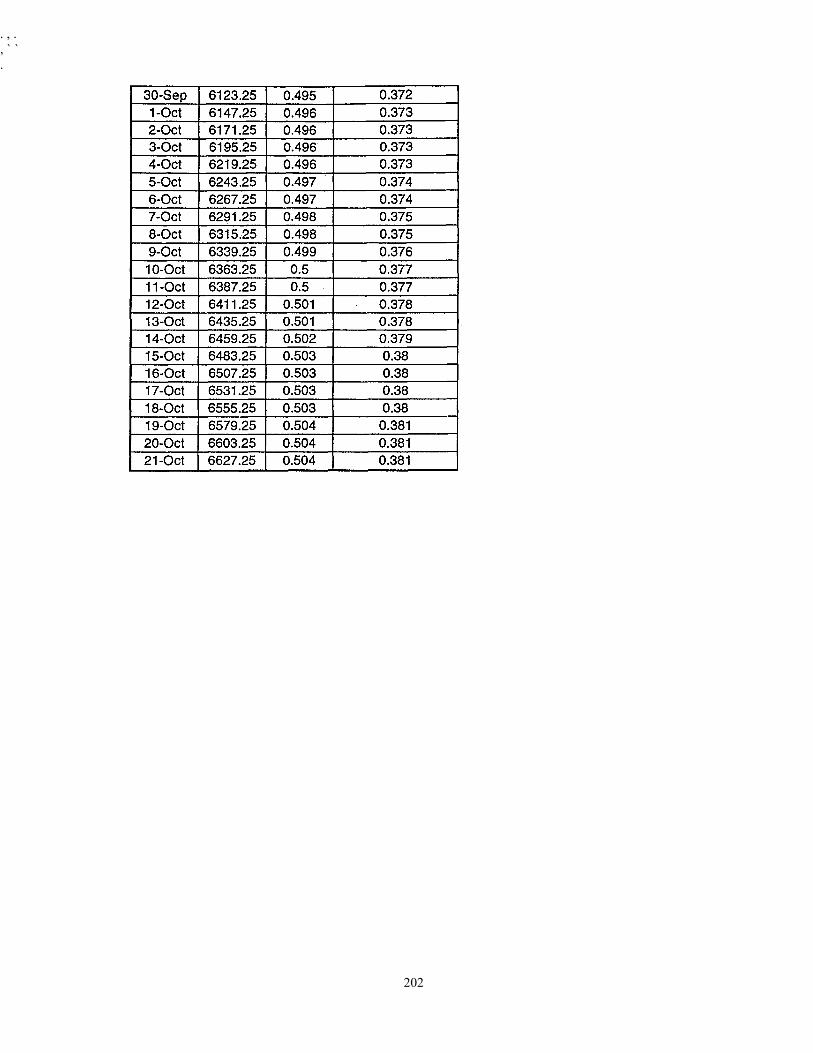
The rates of modulus decay were quite similar for both Type I and Type II

unnotched specimens [Ahn, W., 1998]. The rates of modulus decay were quite similar for

both Type I and Type II notched specimens but less than unnotched specimens. The

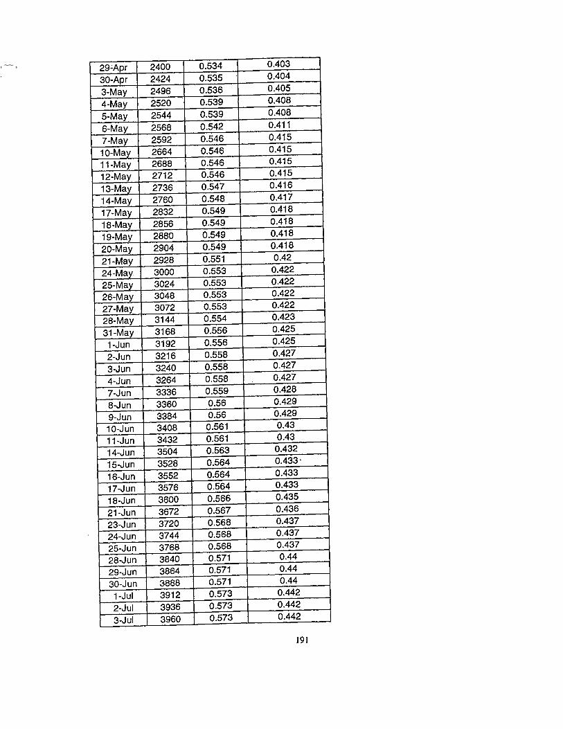
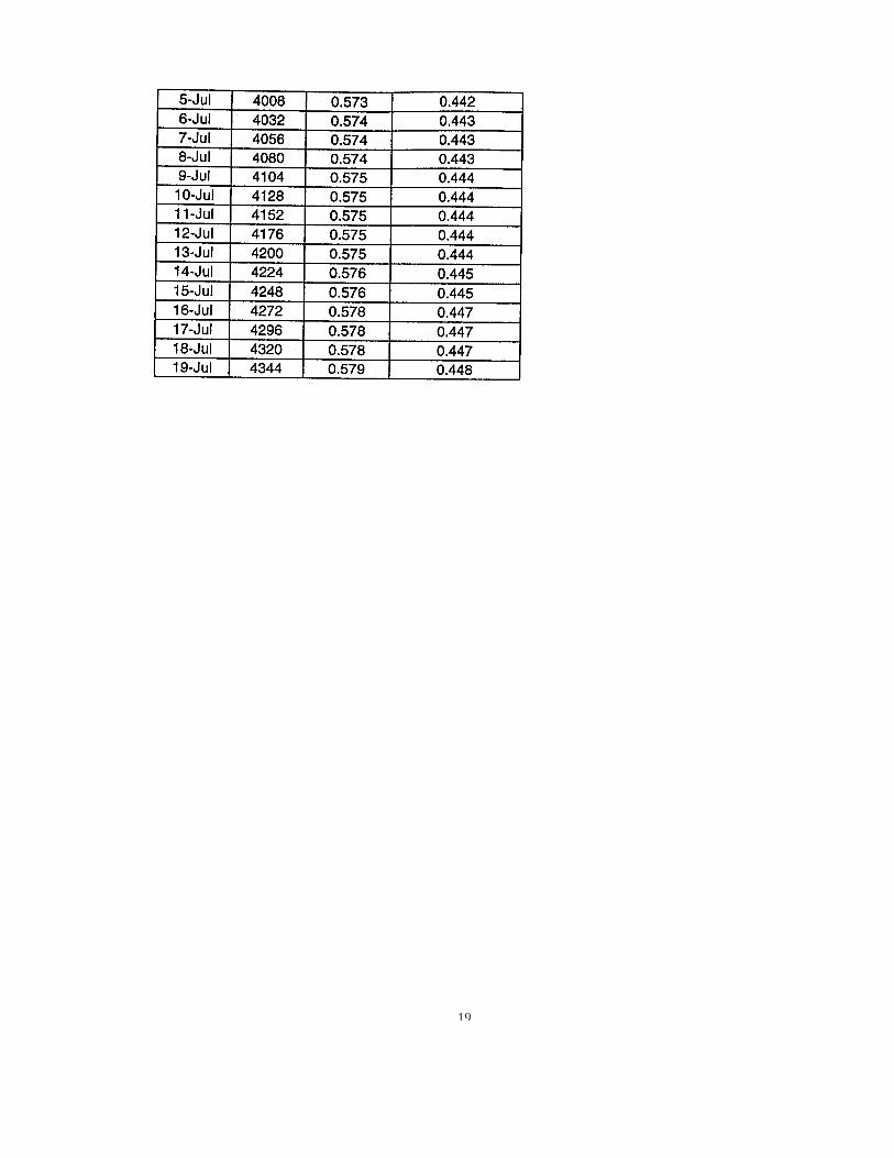
experimental data in the figures is presented in Appendix D.

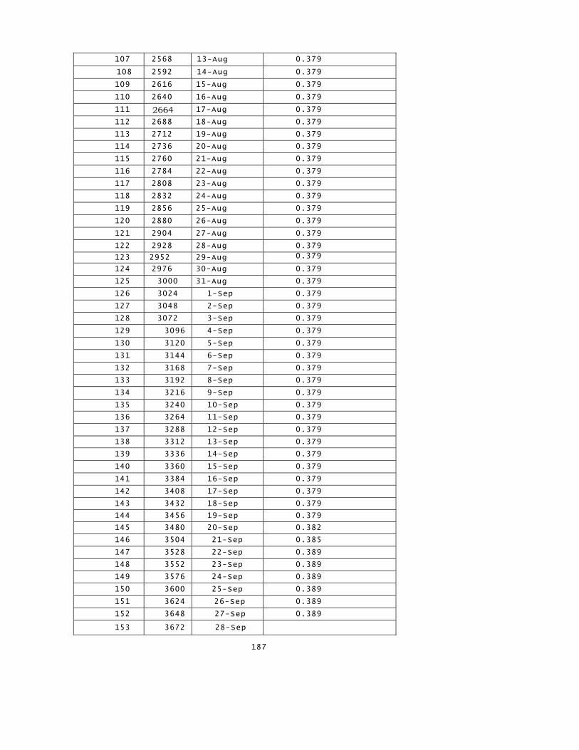
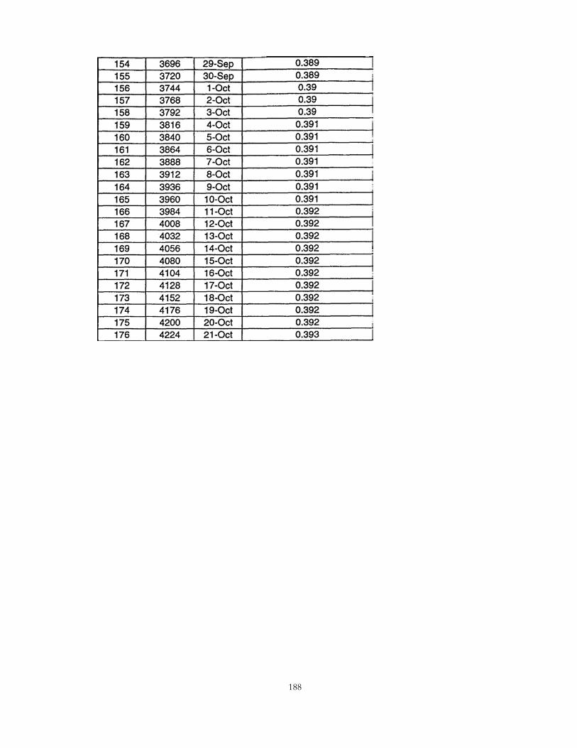
188

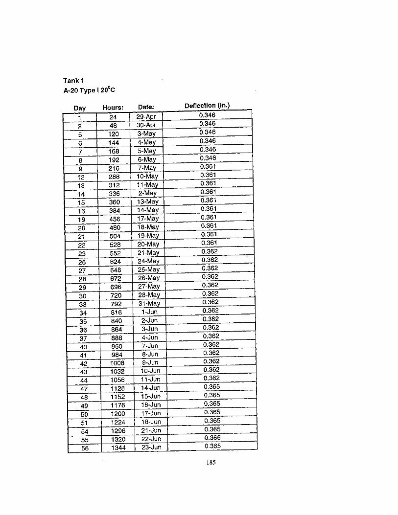
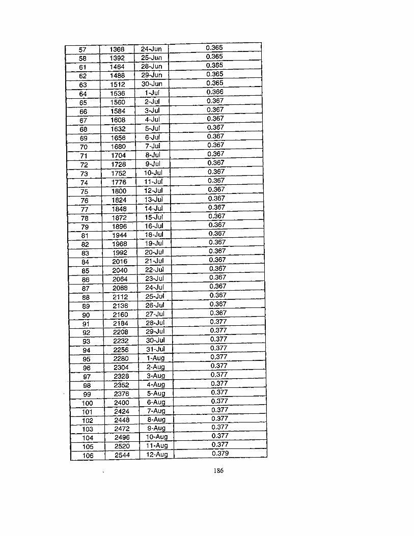
APPENDIX D Data for Flexural Creep Testing of Notched and Un-Notched Pipe Rings

for Enviromental Cracking Resistance

189

107 2568 13-Aug 0.379

108 2592 14-Aug 0.379

109 2616 15-Aug 0.379

110 2640 16-Aug 0.379

111 2664 17-Aug 0.379

112 2688 18-Aug 0.379

113 2712 19-Aug 0.379

114 2736 20-Aug 0.379

115 2760 21-Aug 0.379

116 2784 22-Aug 0.379

117 2808 23-Aug 0.379

118 2832 24-Aug 0.379

119 2856 25-Aug 0.379

120 2880 26-Aug 0.379

121 2904 27-Aug 0.379

122 2928 28-Aug 0.379

123 2952 29-Aug 0.379

124 2976 30-Aug 0.379

125 3000 31-Aug 0.379

126 3024 1-Sep 0.379

127 3048 2-Sep 0.379

128 3072 3-Sep 0.379

129 3096 4-Sep 0.379

130 3120 5-Sep 0.379

131 3144 6-Sep 0.379

132 3168 7-Sep 0.379

133 3192 8-Sep 0.379

134 3216 9-Sep 0.379

135 3240 10-Sep 0.379

136 3264 11-Sep 0.379

137 3288 12-Sep 0.379

138 3312 13-Sep 0.379

139 3336 14-Sep 0.379

140 3360 15-Sep 0.379

141 3384 16-Sep 0.379

142 3408 17-Sep 0.379

143 3432 18-Sep 0.379

144 3456 19-Sep 0.379

145 3480 20-Sep 0.382

146 3504 21-Sep 0.385

147 3528 22-Sep 0.389

148 3552 23-Sep 0.389

149 3576 24-Sep 0.389

150 3600 25-Sep 0.389

151 3624 26-Sep 0.389

152 3648 27-Sep 0.389

153 3672 28-Sep

187

188

, ~~ , .

19

19

19

. , . , ` ` .

202

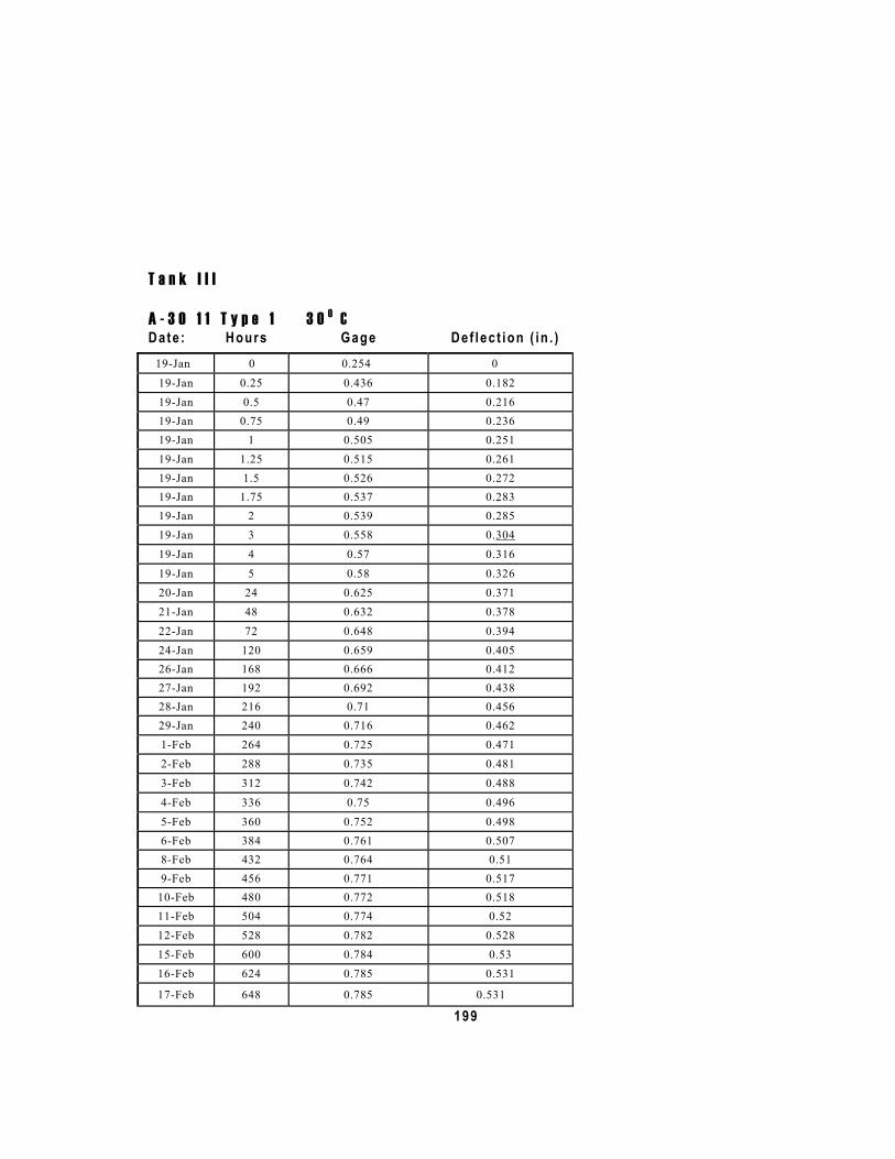
T a n k I I I

A - 3 0 1 1 T y p e 1 3 0 0 C Date : Hours Gage De f lec t ion ( in . )

19-Jan 0 0.254 0

19-Jan 0.25 0.436 0.182 19-Jan 0.5 0.47 0.216 19-Jan 0.75 0.49 0.236 19-Jan 1 0.505 0.251 19-Jan 1.25 0.515 0.261 19-Jan 1.5 0.526 0.272 19-Jan 1.75 0.537 0.283 19-Jan 2 0.539 0.285 19-Jan 3 0.558 0.304

19-Jan 4 0.57 0.316

19-Jan 5 0.58 0.326 20-Jan 24 0.625 0.371 21-Jan 48 0.632 0.378

22-Jan 72 0.648 0.394 24-Jan 120 0.659 0.405 26-Jan 168 0.666 0.412 27-Jan 192 0.692 0.438 28-Jan 216 0.71 0.456 29-Jan 240 0.716 0.462 1-Feb 264 0.725 0.471 2-Feb 288 0.735 0.481

3-Feb 312 0.742 0.488

4-Feb 336 0.75 0.496

5-Feb 360 0.752 0.498 6-Feb 384 0.761 0.507 8-Feb 432 0.764 0.51 9-Feb 456 0.771 0.517

10-Feb 480 0.772 0.518 11-Feb 504 0.774 0.52 12-Feb 528 0.782 0.528 15-Feb 600 0.784 0.53 16-Feb 624 0.785 0.531

17-Feb 648 0.785 0.531

199

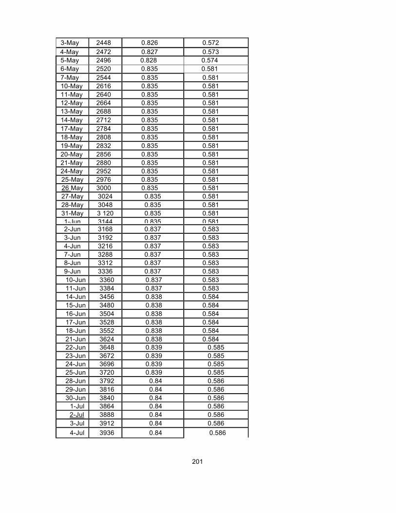
3-May 2448 0.826 0.572 4-May 2472 0.827 0.573 5-May 2496 0.828 0.574 6-May 2520 0.835 0.581 7-May 2544 0.835 0.581 10-May 2616 0.835 0.581 11-May 2640 0.835 0.581 12-May 2664 0.835 0.581 13-May 2688 0.835 0.581 14-May 2712 0.835 0.581 17-May 2784 0.835 0.581 18-May 2808 0.835 0.581 19-May 2832 0.835 0.581 20-May 2856 0.835 0.581 21-May 2880 0.835 0.581 24-May 2952 0.835 0.581 25-May 2976 0.835 0.581 26 May 3000 0.835 0.581 27-May 3024 0.835 0.581 28-May 3048 0.835 0.581 31-May 3 120 0.835 0.581 1-Jun 3144 0.835 0.5812-Jun 3168 0.837 0.583 3-Jun 3192 0.837 0.583 4-Jun 3216 0.837 0.583 7-Jun 3288 0.837 0.583 8-Jun 3312 0.837 0.583 9-Jun 3336 0.837 0.583 10-Jun 3360 0.837 0.583 11-Jun 3384 0.837 0.583 14-Jun 3456 0.838 0.584 15-Jun 3480 0.838 0.584 16-Jun 3504 0.838 0.584 17-Jun 3528 0.838 0.584 18-Jun 3552 0.838 0.584 21-Jun 3624 0.838 0.584 22-Jun 3648 0.839 0.585 23-Jun 3672 0.839 0.585 24-Jun 3696 0.839 0.585 25-Jun 3720 0.839 0.585 28-Jun 3792 0.84 0.586 29-Jun 3816 0.84 0.586 30-Jun 3840 0.84 0.586

1-Jul 3864 0.84 0.586 2-Jul 3888 0.84 0.586 3-Jul 3912 0.84 0.586 4-Jul 3936 0.84 0.586

201

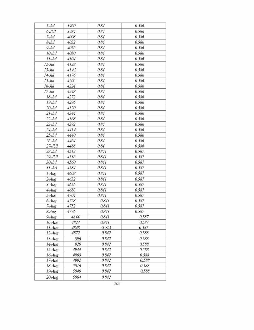
5-Jul 3960 0.84 0.586 6-JUI 3984 0.84 0.5867-Jul 4008 0.84 0.5868-Jul 4032 0.84 0.586 9-Jul 4056 0.84 0.586 10-Jul 4080 0.84 0.586 11-Jul 4104 0.84 0.586

12-Jul 4128 0.84 0.586 13-Jul 41 b2 0.84 0.58614-Jul 4176 0.84 0.586 15-Jul 4200 0.84 0.58616-Jul 4224 0.84 0.58617-Jul 4248 0.84 0.586

18-Jul 4272 0.84 0.58619-Jul 4296 0.84 0.586 20-Jul 4320 0.84 0.586 21-Jul 4344 0.84 0.586 22-Jul 4368 0.84 0.586 23-Jul 4392 0.84 0,58624-Jul 441 6 0.84 0.586 25-Jul 4440 0.84 0.586 26-Jul 4464 0.84 0.58627-JUI 4488 0.84 0.58628-Jul 4512 0.841 0.58729-JUI 4536 0.841 0.58730-Jul 4560 0.841 0.587 31-Ju1 4584 0.841 0.5871-Aug 4608 0.841 0.587 2-Aug 4632 0.841 0.587 3-Aug 4656 0.841 0.5874-Aug 4680 0.841 0.5875-Aug 4704 0.841 0.5876-Aug 4728 0.841 0.5877-Aug 4752 0.841 0.587 8.Aug 4776 0.841 0.5879-Aug 48 00 0.841 0.587 10-Aug 4824 0.841 0.58711-Aug 4848 0 .841 . 0.58712-Aug 4872 0.842 0.588 13-Aug 896 0.842 0.588 14-Aug 920 0.842 0.588 15-Aug 4944 0.842 0.588 16-Aug 4968 0.842 0.58817-Aug 4992 0.842 0:588 18-Aug 5016 0.842 0.588 19-Aug 5040 0.842 0.58820-Aug 5064 0.842

202

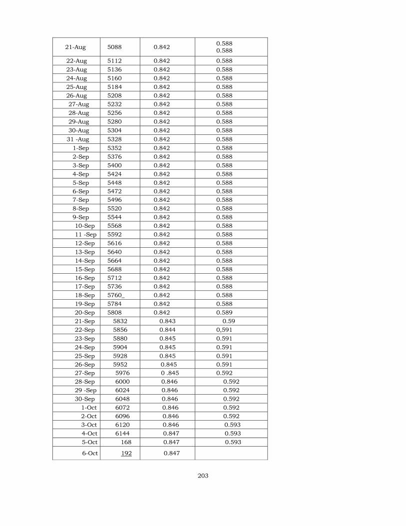
21-Aug 5088 0.842 0.588 0.588

22-Aug 5112 0.842 0.588 23-Aug 5136 0.842 0.588 24-Aug 5160 0.842 0.588 25-Aug 5184 0.842 0.588 26-Aug 5208 0.842 0.588 27-Aug 5232 0.842 0.588 28-Aug 5256 0.842 0.588 29-Aug 5280 0.842 0.588 30-Aug 5304 0.842 0.588 31 -Aug 5328 0.842 0.588

1-Sep 5352 0.842 0.588 2-Sep 5376 0.842 0.588 3-Sep 5400 0.842 0.588 4-Sep 5424 0.842 0.588 5-Sep 5448 0.842 0.588 6-Sep 5472 0.842 0.588 7-Sep 5496 0.842 0.588 8-Sep 5520 0.842 0.588 9-Sep 5544 0.842 0.588 10-Sep 5568 0.842 0.588 11 -Sep 5592 0.842 0.588 12-Sep 5616 0.842 0.588 13-Sep 5640 0.842 0.588 14-Sep 5664 0.842 0.588 15-Sep 5688 0.842 0.588 16-Sep 5712 0.842 0.588 17-Sep 5736 0.842 0.588 18-Sep 5760_ 0.842 0.588 19-Sep 5784 0.842 0.588 20-Sep 5808 0.842 0.589 21-Sep 5832 0.843 0.59 22-Sep 5856 0.844 0,591 23-Sep 5880 0.845 0.591 24-Sep 5904 0.845 0.591 25-Sep 5928 0.845 0.591 26-Sep 5952 0.845 0.591 27-Sep 5976 0 .845 0.592 28-Sep 6000 0.846 0.592 29 -Sep 6024 0.846 0.592 30-Sep 6048 0.846 0.592

1-Oct 6072 0.846 0.592 2-Oct 6096 0.846 0.592 3-Oct 6120 0.846 0.593 4-Oct 6144 0.847 0.593 5-Oct 168 0.847 0.593

6-Oct 192 0.847

203

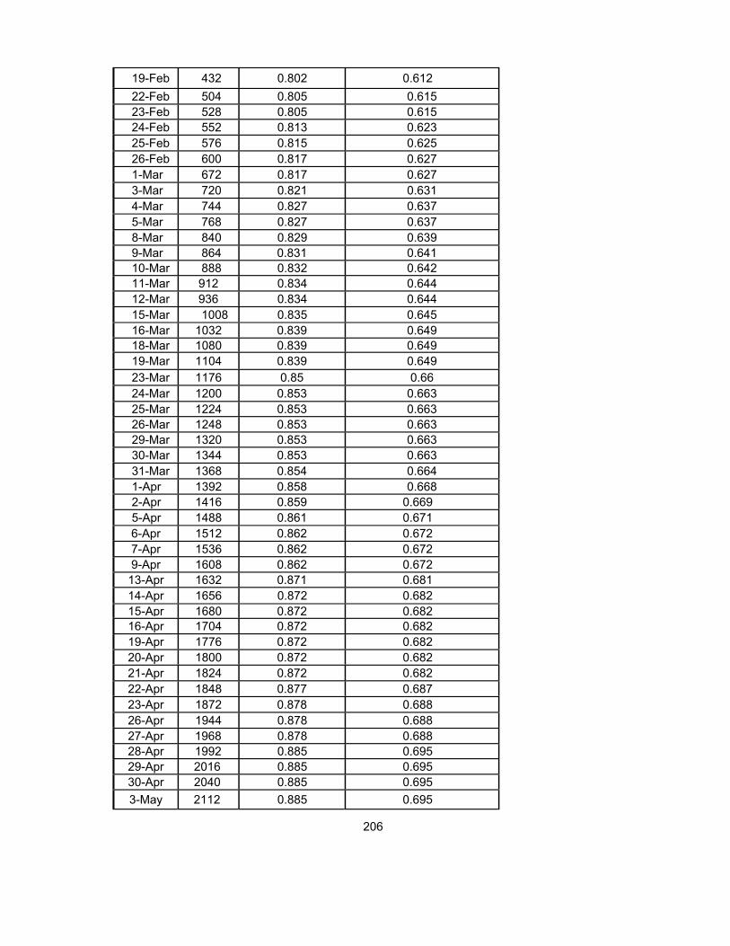
19-Feb 432 0.802 0.612 22-Feb 504 0.805 0.615 23-Feb 528 0.805 0.615 24-Feb 552 0.813 0.623 25-Feb 576 0.815 0.625 26-Feb 600 0.817 0.627 1-Mar 672 0.817 0.627 3-Mar 720 0.821 0.631 4-Mar 744 0.827 0.637 5-Mar 768 0.827 0.637 8-Mar 840 0.829 0.639 9-Mar 864 0.831 0.641 10-Mar 888 0.832 0.642 11-Mar 912 0.834 0.644 12-Mar 936 0.834 0.644 15-Mar 1008 0.835 0.645 16-Mar 1032 0.839 0.649 18-Mar 1080 0.839 0.64919-Mar 1104 0.839 0.649 23-Mar 1176 0.85 0.66 24-Mar 1200 0.853 0.663 25-Mar 1224 0.853 0.663 26-Mar 1248 0.853 0.663 29-Mar 1320 0.853 0.663 30-Mar 1344 0.853 0.663 31-Mar 1368 0.854 0.664 1-Apr 1392 0.858 0.668 2-Apr 1416 0.859 0.669 5-Apr 1488 0.861 0.671 6-Apr 1512 0.862 0.672 7-Apr 1536 0.862 0.672 9-Apr 1608 0.862 0.672

13-Apr 1632 0.871 0.681 14-Apr 1656 0.872 0.682 15-Apr 1680 0.872 0.682 16-Apr 1704 0.872 0.682 19-Apr 1776 0.872 0.682 20-Apr 1800 0.872 0.682 21-Apr 1824 0.872 0.682 22-Apr 1848 0.877 0.687 23-Apr 1872 0.878 0.688 26-Apr 1944 0.878 0.688 27-Apr 1968 0.878 0.688 28-Apr 1992 0.885 0.695 29-Apr 2016 0.885 0.695 30-Apr 2040 0.885 0.695 3-May 2112 0.885 0.695

206

4-May __2j _36 0.885 0.695 5-May 2160 0.888 0.698 6-May 2184 0.888 0.698 7-May 2208 0.888 0.698

10-May 2280 0.888 0.698 11-May 2304 0.888 0.698 12-May 2328 0.888 0.698 13-May 235 0.888 0.69814-May 2376 0.888 0.698 17-May 2448 0.888 0.69818-May 2472 0.888 0.698 19-May 2496 0.888 0.698 20-May 2520 0.888 0.698 21-May 2544 0.889 0.699 24-May 2616 0.889 0.699 25-May 2640 0.889 0.699 26-May 2664 0.889 0.699 27-May 2688 0.889 0.69928-May 2712 0.889 0.699 31-May 2784 0.889 0.699

1-Jun 2808 0.889 0.6992-Jun 2832 0.889 0.699 3-Jun 2856 0.889 0.699 4-Jun 2880 0.889 0.699 7-Jun 2952 0.889 0.699 8-Jun 2976 0.889 0.699 9-Jun 3000 0.889 0.699 10-Jun 3024 0.89 0.711-Jun 3048 0.898 0.708 14 Jun 3120 0.899 0.70915-Jun 3144 0.899 0.709 16-Jun 3168 0.901 0.711 17-Jun 3192 0.901 0.711 18-Jun 3216 0.901 0.711 21-Jun 3288 0.901 0.711 22-Jun 3312 0.901 0.711 23-Jun 3336 0.901 0.711 24-Jun 3360 0.901 0.711 25-Jun 3384 0.901 0.711 28-Jun 3456 0.902 0.712 29-Jun 3480 0.902 0.712 30-Jun 3504 0.902 0.712

1-Jul 3528 0.902 0.712 2-Jul 3552 0.903 0.713 3-Jul 3576 0.903 0.713 4-Jul 3600 0.903 0.713 5 Jul 3624 0 .903 0.713 l

207

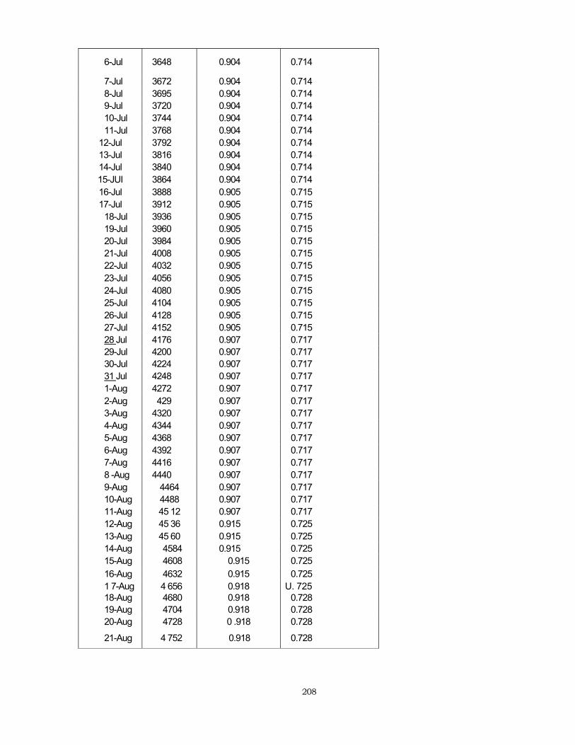
6-Jul 3648 0.904 0.714

7-Jul 3672 0.904 0.714 8-Jul 3695 0.904 0.714 9-Jul 3720 0.904 0.714 10-Jul 3744 0.904 0.714 11-Jul 3768 0.904 0.714

12-Jul 3792 0.904 0.714 13-Jul 3816 0.904 0.714 14-Jul 3840 0.904 0.714 15-JUI 3864 0.904 0.714 16-Jul 3888 0.905 0.715 17-Jul 3912 0.905 0.715

18-Jul 3936 0.905 0.715 19-Jul 3960 0.905 0.715 20-Jul 3984 0.905 0.715 21-Jul 4008 0.905 0.715 22-Jul 4032 0.905 0.715 23-Jul 4056 0.905 0.715 24-Jul 4080 0.905 0.715 25-Jul 4104 0.905 0.715 26-Jul 4128 0.905 0.715 27-Jul 4152 0.905 0.715 28 Jul 4176 0.907 0.717 29-Jul 4200 0.907 0.717 30-Jul 4224 0.907 0.717 31 Jul 4248 0.907 0.717 1-Aug 4272 0.907 0.717 2-Aug 429 0.907 0.717 3-Aug 4320 0.907 0.717 4-Aug 4344 0.907 0.717 5-Aug 4368 0.907 0.717 6-Aug 4392 0.907 0.717 7-Aug 4416 0.907 0.717 8 -Aug 4440 0.907 0.717 9-Aug 4464 0.907 0.717 10-Aug 4488 0.907 0.717 11-Aug 45 12 0.907 0.717 12-Aug 45 36 0.915 0.725 13-Aug 45 60 0.915 0.725 14-Aug 4584 0.915 0.725 15-Aug 4608 0.915 0.725 16-Aug 4632 0.915 0.725 1 7-Aug 4 656 0.918 U. 725 18-Aug 4680 0.918 0.728 19-Aug 4704 0.918 0.728 20-Aug 4728 0 .918 0.728

21-Aug 4 752 0.918 0.728

208

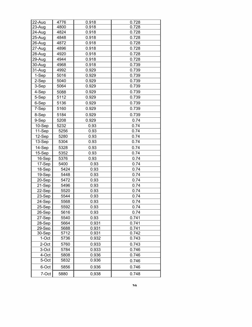
22-Aug 4776 0.918 0.728 23-Aug 4800 0.918 0.728 24-Aug 4824 0.918 0.728 25-Aug 4848 0.918 0.728 26-Aug 4872 0.918 0.728 27-Aug 4896 0.918 0.728 28-Aug 4920 0.918 0.728 29-Aug 4944 0.918 0.728 30-Aug 4968 0.918 0.739 31-Aug 4992 0.929 0.739

1-Sep 5016 0.929 0.739 2-Sep 5040 0.929 0.739 3-Sep 5064 0.929 0.739 4-Sep 5088 0.929 0.739 5-Sep 5112 0.929 0.739 6-Sep 5136 0.929 0.739 7-Sep 5160 0.929 0.739 8-Sep 5184 0.929 0.739 9-Sep 5208 0.929 0.74 10-Sep 5232 0.93 0.74 11-Sep 5256 0.93 0.74 12-Sep 5280 0.93 0.74 13-Sep 5304 0.93 0.74 14-Sep 5328 0.93 0.74 15-Sep 5352 0.93 0.74 16-Sep 5376 0.93 0.74 17-Sep 5400 0.93 0.74 18-Sep 5424 0.93 0.74 19-Sep 5448 0.93 0.74 20-Sep 5472 0.93 0.74 21-Sep 5496 0.93 0.74 22-Sep 5520 0.93 0.74 23-Sep 5544 0.93 0.74 24-Sep 5568 0.93 0.74 25-Sep 5592 0.93 0.74 26-Sep 5616 0.93 0.74 27-Sep 5540 0.93 0.741 28-Sep 5664 0.931 0.741 29-Sep 5688 0.931 0.741 30-Sep 5712 0.931 0.742

1-Oct 5736 0.932 0.743 2-Oct 5760 0.933 0.743 3-Oct 5784 0.933 0.746 4-Oct 5808 0.936 0.746 5-Oct 5832 0.936 0.746 6-Oct 5856 0.936 0.746 7-Oct 5880 0,938 0.748

20

8-Oct 5904 0.938 0.148 9-Oct 5928 1939 0.749

1 O-Oct 5952 0.94 0.75 11 -Oct 5976 0.941 0.751 12-Oct 6000 0.941 0.751 13-Oct 6024 1941 0.151 14-Oct 6048 0.942 0.752 15-oct 6072 0.942 0.752 16-Oct 6096 0.942 0.752 17-Oct 6120 0.943 0.753 18-Oct 6144 0.943 0.753 19-Oct 6168 0.943 0.153 20-Oct 6192 0.943 0.753 21-OW

16216 0. 0.754

2l0

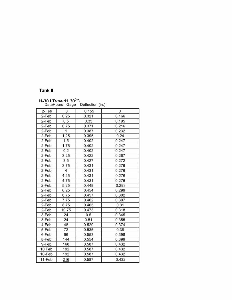
Tank II

H-30 I Type 11 300CDateHours Gage Deflection (in.)

2-Feb 0 0.155 0 2-Feb 0.25 0.321 0.166 2-Feb 0.5 0.35 0.195 2-Feb 0.75 0.371 0.216 2-Feb 1 0.387 0.232 2-Feb 1.25 0.395 0.24 2-Feb 1.5 0.402 0.247 2-Feb 1.75 0.402 0.247 2-Feb 0.2 0.402 0.247 2-Feb 3.25 0.422 0.267 2-Feb 3.5 0.427 0.272 2-Feb 3.75 0.431 0.276 2-Feb 4 0.431 0.276 2-Feb 4.25 0.431 0.276 2-Feb 4.75 0.431 0.276 2-Feb 5.25 0.448 0.293 2-Feb 6.25 0.454 0.299 2-Feb 6.75 0.457 0.302 2-Feb 7.75 0.462 0.307 2-Feb 8.75 0.465 0.31 2-Feb 10.75 0.473 0.318 3-Feb 24 0.5 0.345 3-Feb 24 0.51 0.355 4-Feb 48 0.529 0.374 5-Feb 72 0.535 0.38 6-Feb 96 0.553 0.398 8-Feb 144 0.554 0.399 9-Feb 168 0.587 0.432 10 Feb 192 0.587 0.432 10-Feb 192 0.587 0.432 11-Feb 216 0.587 0.432

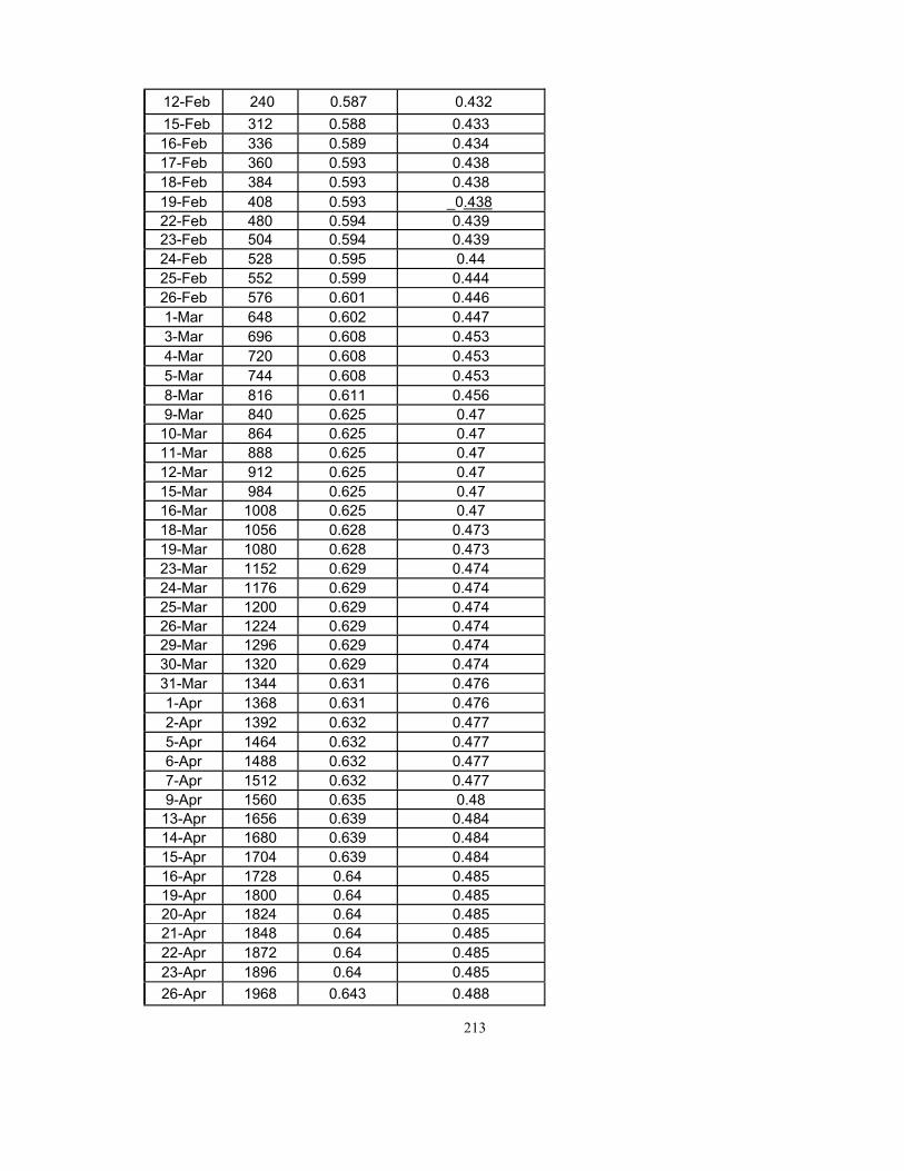
12-Feb 240 0.587 0.432 15-Feb 312 0.588 0.433 16-Feb 336 0.589 0.434 17-Feb 360 0.593 0.438 18-Feb 384 0.593 0.438 19-Feb 408 0.593 _0.438 22-Feb 480 0.594 0.439 23-Feb 504 0.594 0.439 24-Feb 528 0.595 0.44 25-Feb 552 0.599 0.444 26-Feb 576 0.601 0.446 1-Mar 648 0.602 0.447 3-Mar 696 0.608 0.453 4-Mar 720 0.608 0.453 5-Mar 744 0.608 0.453 8-Mar 816 0.611 0.456 9-Mar 840 0.625 0.47

10-Mar 864 0.625 0.47 11-Mar 888 0.625 0.47 12-Mar 912 0.625 0.47 15-Mar 984 0.625 0.47 16-Mar 1008 0.625 0.47 18-Mar 1056 0.628 0.473 19-Mar 1080 0.628 0.473 23-Mar 1152 0.629 0.474 24-Mar 1176 0.629 0.474 25-Mar 1200 0.629 0.474 26-Mar 1224 0.629 0.474 29-Mar 1296 0.629 0.474 30-Mar 1320 0.629 0.474 31-Mar 1344 0.631 0.476 1-Apr 1368 0.631 0.476 2-Apr 1392 0.632 0.477 5-Apr 1464 0.632 0.477 6-Apr 1488 0.632 0.477 7-Apr 1512 0.632 0.477 9-Apr 1560 0.635 0.48

13-Apr 1656 0.639 0.484 14-Apr 1680 0.639 0.484 15-Apr 1704 0.639 0.484 16-Apr 1728 0.64 0.485 19-Apr 1800 0.64 0.485 20-Apr 1824 0.64 0.485 21-Apr 1848 0.64 0.485 22-Apr 1872 0.64 0.485 23-Apr 1896 0.64 0.485 26-Apr 1968 0.643 0.488

213

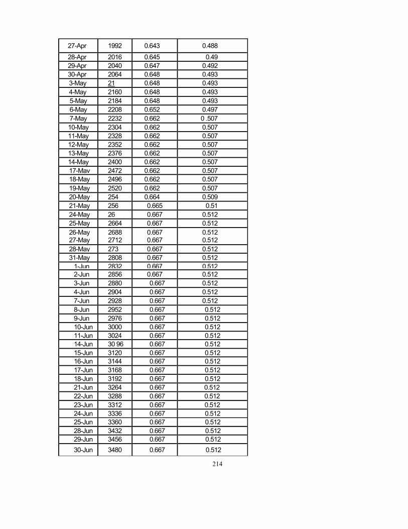
27-Apr 1992 0.643 0.488 28-Apr 2016 0.645 0.49 29-Apr 2040 0.647 0.492 30-Apr 2064 0.648 0.493 3-May 21 0.648 0.493 4-May 2160 0.648 0.493 5-May 2184 0.648 0.493 6-May 2208 0.652 0.497 7-May 2232 0.662 0 .507 10-May 2304 0.662 0.507 11-May 2328 0.662 0.507 12-May 2352 0.662 0.507 13-May 2376 0.662 0.507 14-May 2400 0.662 0.507 17-May 2472 0.662 0.50718-May 2496 0.662 0.507 19-May 2520 0.662 0.507 20-May 254 0.664 0.509 21-May 256 0.665 0.51 24-May 26 0.667 0.512 25-May 2664 0.667 0.512 26-May 27-May

2688 2712

0.667 0.667

0.512 0.512

28-May 273 0.667 0.51231-May 2808 0.667 0.512

1-Jun 2832 0.667 0.5122-Jun 2856 0.667 0.512 3-Jun 2880 0.667 0.512 4-Jun 2904 0.667 0.512 7-Jun 2928 0.667 0.512 8-Jun 2952 0.667 0.512 9-Jun 2976 0.667 0.512 10-Jun 3000 0.667 0.512 11-Jun 3024 0.667 0.51214-Jun 30 96 0.667 0.512 15-Jun 3120 0.667 0.51216-Jun 3144 0.667 0.512 17-Jun 3168 0.667 0.512 18-Jun 3192 0.667 0.512 21-Jun 3264 0.667 0.512 22-Jun 3288 0.667 0.512 23-Jun 3312 0.667 0.512 24-Jun 3336 0.667 0.512 25-Jun 3360 0.667 0.512 28-Jun 3432 0.667 0.512 29-Jun 3456 0.667 0.512 30-Jun 3480 0.667 0.512

214

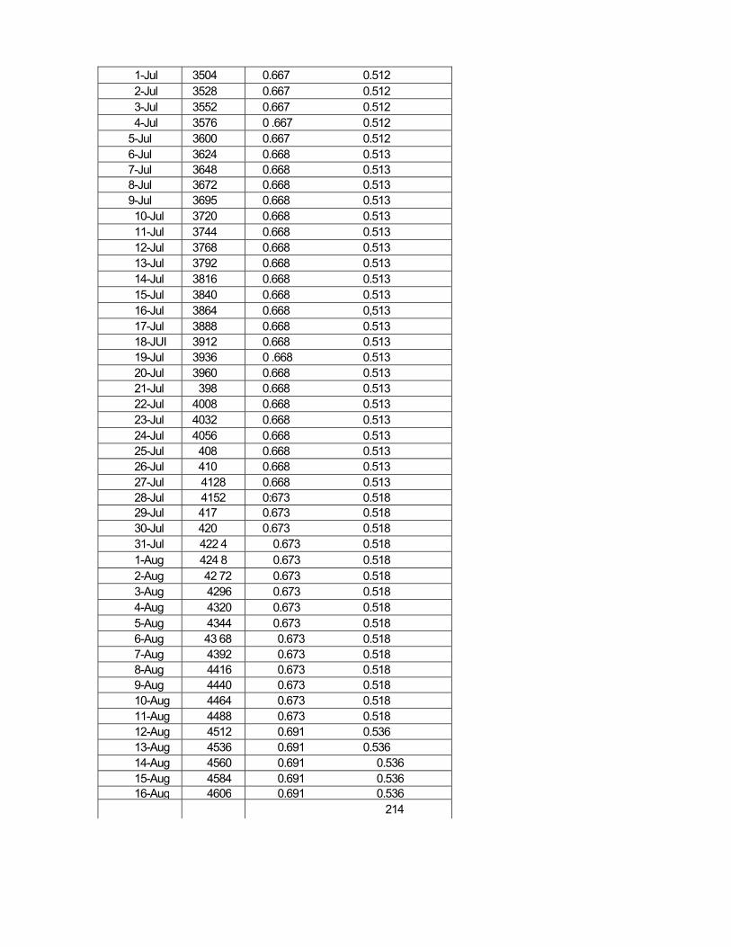
1-Jul 3504 0.667 0.512 2-Jul 3528 0.667 0.512 3-Jul 3552 0.667 0.512 4-Jul 3576 0 .667 0.512

5-Jul 3600 0.667 0.512 6-Jul 3624 0.668 0.513 7-Jul 3648 0.668 0.513 8-Jul 3672 0.668 0.513 9-Jul 3695 0.668 0.513 10-Jul 3720 0.668 0.513 11-Jul 3744 0.668 0.513 12-Jul 3768 0.668 0.513 13-Jul 3792 0.668 0.513 14-Jul 3816 0.668 0.513 15-Jul 3840 0.668 0.513 16-Jul 3864 0.668 0,513 17-Jul 3888 0.668 0.513 18-JUI 3912 0.668 0.513 19-Jul 3936 0 .668 0.513 20-Jul 3960 0.668 0.513 21-Jul 398 0.668 0.513 22-Jul 4008 0.668 0.513 23-Jul 4032 0.668 0.513 24-Jul 4056 0.668 0.513 25-Jul 408 0.668 0.513 26-Jul 410 0.668 0.513 27-Jul 4128 0.668 0.513 28-Jul 4152 0:673 0.518 29-Jul 417 0.673 0.518 30-Jul 420 0.673 0.518 31-Jul 422 4 0.673 0.518 1-Aug 424 8 0.673 0.518 2-Aug 42 72 0.673 0.518 3-Aug 4296 0.673 0.518 4-Aug 4320 0.673 0.518 5-Aug 4344 0.673 0.518 6-Aug 43 68 0.673 0.518 7-Aug 4392 0.673 0.518 8-Aug 4416 0.673 0.518 9-Aug 4440 0.673 0.518 10-Aug 4464 0.673 0.518 11-Aug 4488 0.673 0.518 12-Aug 4512 0.691 0.536 13-Aug 4536 0.691 0.536 14-Aug 4560 0.691 0.536 15-Aug 4584 0.691 0.536 16-Aug 4606 0.691 0.536

214

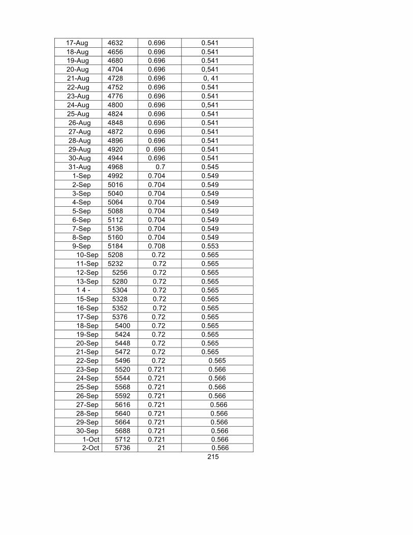
17-Aug 4632 0.696 0.541 18-Aug 4656 0.696 0.541 19-Aug 4680 0.696 0.541 20-Aug 4704 0.696 0,541 21-Aug 4728 0.696 0, 41 22-Aug 4752 0.696 0.541 23-Aug 4776 0.696 0.541 24-Aug 4800 0.696 0,541 25-Aug 4824 0.696 0.541 26-Aug 4848 0.696 0.541 27-Aug 4872 0.696 0.541 28-Aug 4896 0.696 0.541 29-Aug 4920 0 .696 0.541 30-Aug 4944 0.696 0.541 31-Aug 4968 0.7 0.545

1-Sep 4992 0.704 0.549 2-Sep 5016 0.704 0.549 3-Sep 5040 0.704 0.549 4-Sep 5064 0.704 0.549 5-Sep 5088 0.704 0.549 6-Sep 5112 0.704 0.549 7-Sep 5136 0.704 0.549 8-Sep 5160 0.704 0.549 9-Sep 5184 0.708 0.553

10-Sep 5208 0.72 0.565 11-Sep 5232 0.72 0.565 12-Sep 5256 0.72 0.565 13-Sep 5280 0.72 0.565 1 4 - 5304 0.72 0.565 15-Sep 5328 0.72 0.565 16-Sep 5352 0.72 0.565 17-Sep 5376 0.72 0.565 18-Sep 5400 0.72 0.565 19-Sep 5424 0.72 0.565 20-Sep 5448 0.72 0.565 21-Sep 5472 0.72 0.565 22-Sep 5496 0.72 0.565 23-Sep 5520 0.721 0.566 24-Sep 5544 0.721 0.566 25-Sep 5568 0.721 0.566 26-Sep 5592 0.721 0.566 27-Sep 5616 0.721 0.566 28-Sep 5640 0.721 0.566 29-Sep 5664 0.721 0.566 30-Sep 5688 0.721 0.566

1-Oct 5712 0.721 0.566 2-Oct 5736 21 0.566

215

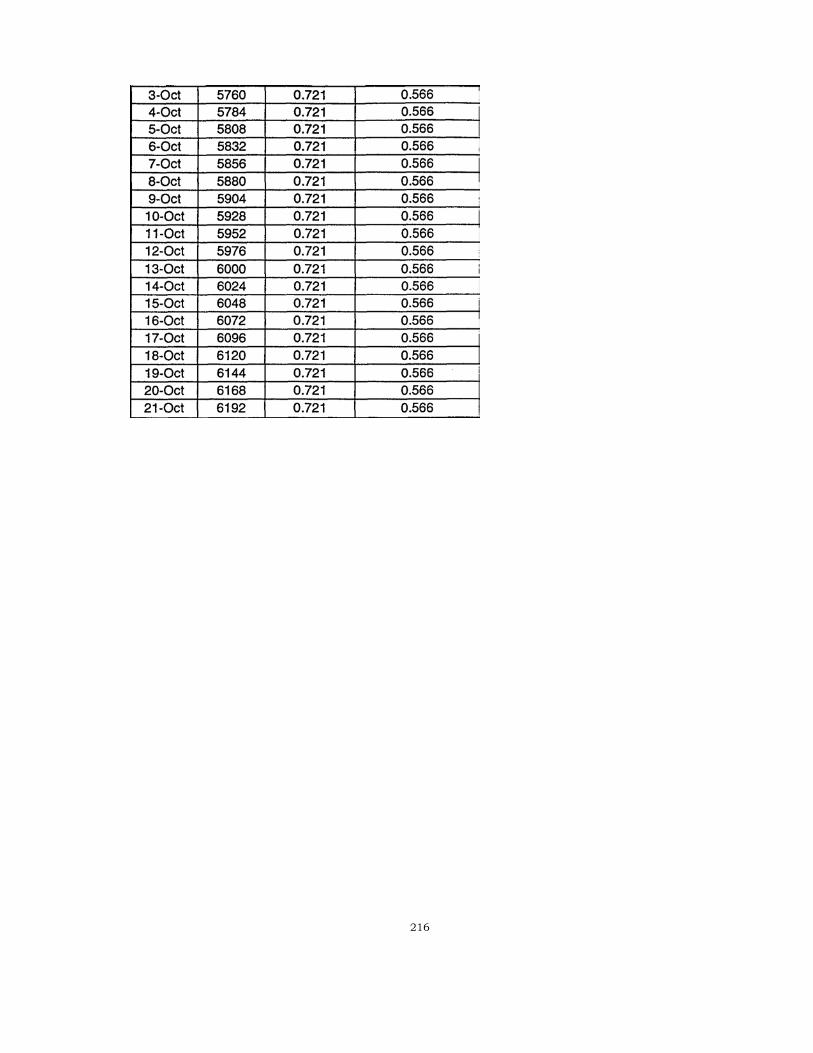
216

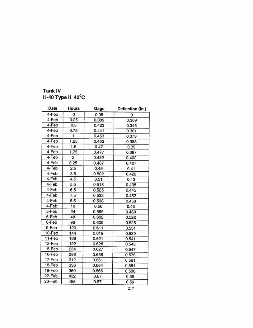
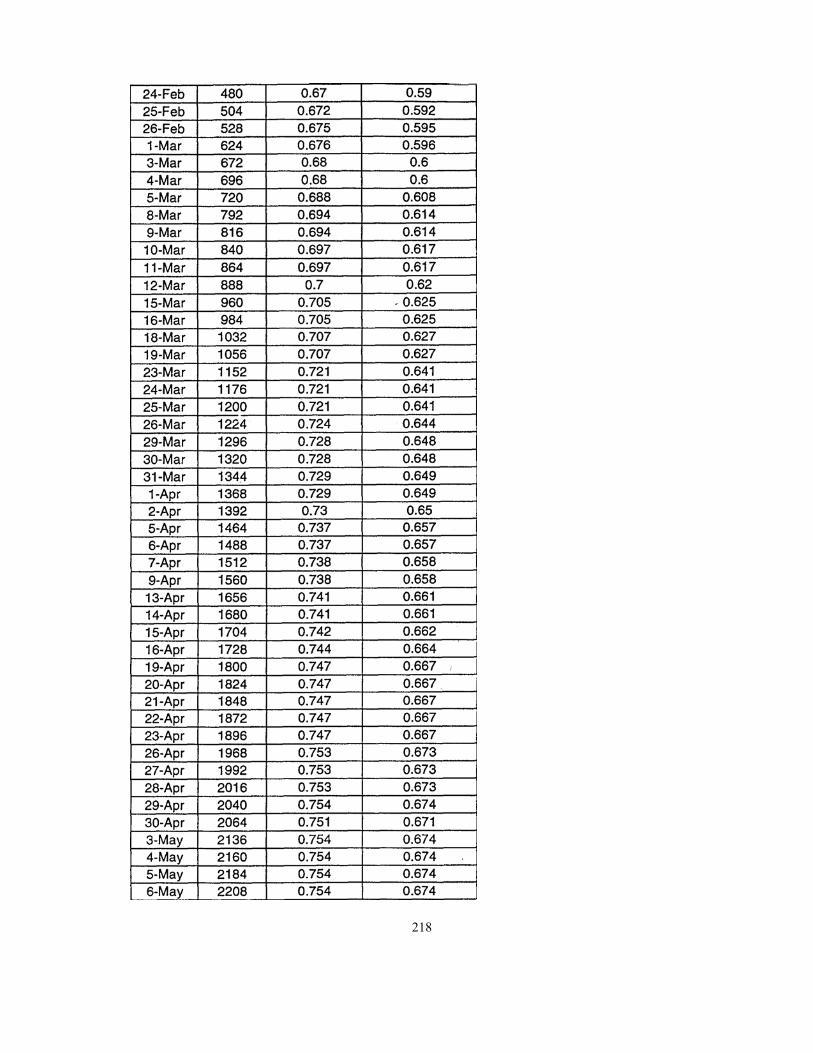
218

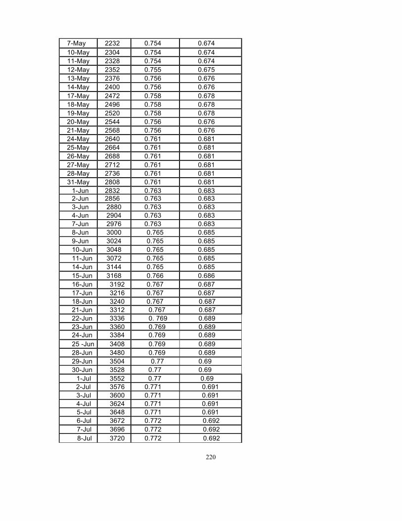
7-May 2232 0.754 0.674 10-May 2304 0.754 0.674 11-May 2328 0.754 0.674 12-May 2352 0.755 0.675 13-May 2376 0.756 0.676 14-May 2400 0.756 0.676 17-May 2472 0.758 0.678 18-May 2496 0.758 0.678 19-May 2520 0.758 0.678 20-May 2544 0.756 0.676 21-May 2568 0.756 0.676 24-May 2640 0.761 0.681 25-May 2664 0.761 0.681 26-May 2688 0.761 0.681 27-May 2712 0.761 0.681 28-May 2736 0.761 0.681 31-May 2808 0.761 0.681

1-Jun 2832 0.763 0.683 2-Jun 2856 0.763 0.683 3-Jun 2880 0.763 0.683 4-Jun 2904 0.763 0.683 7-Jun 2976 0.763 0.683 8-Jun 3000 0.765 0.685 9-Jun 3024 0.765 0.685 10-Jun 3048 0.765 0.685 11-Jun 3072 0.765 0.685 14-Jun 3144 0.765 0.685 15-Jun 3168 0.766 0.686 16-Jun 3192 0.767 0.687 17-Jun 3216 0.767 0.687 18-Jun 3240 0.767 0.68721-Jun 3312 0.767 0.687 22-Jun 3336 0. 769 0.689 23-Jun 3360 0.769 0.68924-Jun 3384 0.769 0.689 25 -Jun 3408 0.769 0.689 28-Jun 3480 0.769 0.689 29-Jun 3504 0.77 0.69 30-Jun 3528 0.77 0.69

1-Jul 3552 0.77 0.69 2-Jul 3576 0.771 0.691 3-Jul 3600 0.771 0.691 4-Jul 3624 0.771 0.691 5-Jul 3648 0.771 0.691 6-Jul 3672 0.772 0.692 7-Jul 3696 0.772 0.692 8-Jul 3720 0.772 0.692

220

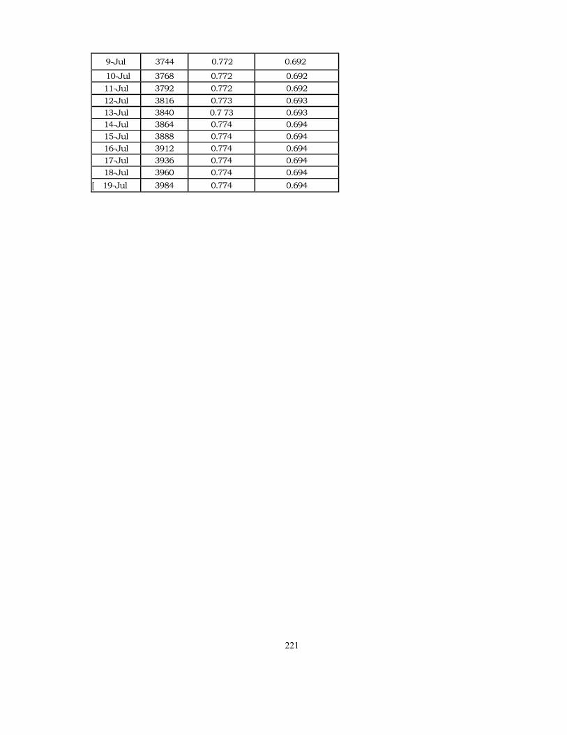
9-Jul 3744 0.772 0.692

10-Jul 3768 0.772 0.692 11-Jul 3792 0.772 0.692 12-Jul 3816 0.773 0.693 13-Jul 3840 0.7 73 0.693 14-Jul 3864 0.774 0.694 15-Jul 3888 0.774 0.694 16-Jul 3912 0.774 0.694 17-Jul 3936 0.774 0.694 18-Jul 3960 0.774 0.694

[ 19-Jul 3984 0.774 0.694

221

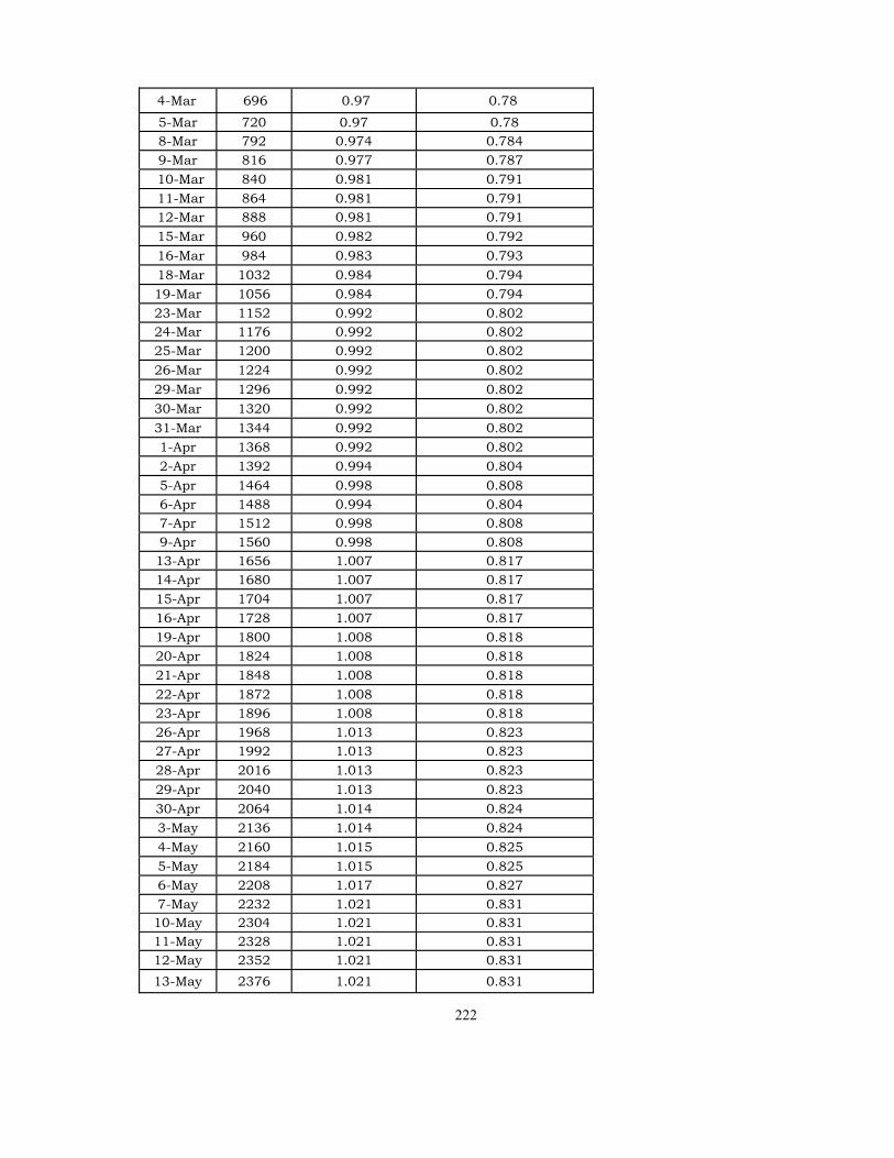
4-Mar 696 0.97 0.78

5-Mar 720 0.97 0.78 8-Mar 792 0.974 0.784 9-Mar 816 0.977 0.787 10-Mar 840 0.981 0.791 11-Mar 864 0.981 0.791 12-Mar 888 0.981 0.791 15-Mar 960 0.982 0.792 16-Mar 984 0.983 0.793 18-Mar 1032 0.984 0.794 19-Mar 1056 0.984 0.794 23-Mar 1152 0.992 0.802 24-Mar 1176 0.992 0.802 25-Mar 1200 0.992 0.802 26-Mar 1224 0.992 0.802 29-Mar 1296 0.992 0.802 30-Mar 1320 0.992 0.802 31-Mar 1344 0.992 0.802 1-Apr 1368 0.992 0.802 2-Apr 1392 0.994 0.804 5-Apr 1464 0.998 0.808 6-Apr 1488 0.994 0.804 7-Apr 1512 0.998 0.808 9-Apr 1560 0.998 0.808 13-Apr 1656 1.007 0.817 14-Apr 1680 1.007 0.817 15-Apr 1704 1.007 0.817 16-Apr 1728 1.007 0.817 19-Apr 1800 1.008 0.818 20-Apr 1824 1.008 0.818 21-Apr 1848 1.008 0.818 22-Apr 1872 1.008 0.818 23-Apr 1896 1.008 0.818 26-Apr 1968 1.013 0.823 27-Apr 1992 1.013 0.823 28-Apr 2016 1.013 0.823 29-Apr 2040 1.013 0.823 30-Apr 2064 1.014 0.824 3-May 2136 1.014 0.824 4-May 2160 1.015 0.825 5-May 2184 1.015 0.825 6-May 2208 1.017 0.827 7-May 2232 1.021 0.831 10-May 2304 1.021 0.831 11-May 2328 1.021 0.831 12-May 2352 1.021 0.831 13-May 2376 1.021 0.831

222

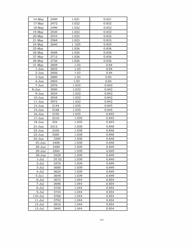
14-May 2400 1.021 0.831 17-May 2472 1.022 0.832 18-May 2496 1.022 0.832 19-May 2520 1.022 0.832 20-May 2544 1.022 0.832 21-May 2568 1.023 0.833 24-May 2640 1 .025 0.835 25-May 1.026 0.836 26-May 2688 1.026 0.836 27-May 2712 1.026 0.836 28-May 2736 1.026 0.836 31-May 2808 1.03 0.84

1-Jun 2832 1.03 0.842-Jun 2856 1.03 0.84 3-Jun 2880 1.03 0.84 4-Jun 2904 1.03 0.84 7-Jun 2976 1.032 0.842

8-Jun 3000 1.032 0.842 9-Jun 3024 1.032 0.842

10-Jun 3048 1.032 0.842 11-Jun 3072 1.032 0.842 14-Jun 3144 1.035 0.845 15-Jun 3168 1.035 0.845 16-Jun 3192 1.035 0.845 17-Jun 3216 1.035 0.845 18-Jun 324 1.035 0.845 21-Jun 3312 1.038 0.848 22-Jun 3336 1.038 0.848 23-Jun 3360 1.038 0.848 24-Jun 3384 1.038 0.848

25-Jun 3408 1.038 0.848 28-Jun 3480 1.039 0.849 29-Jun 3504 1.039 0.849 30-Jun 3528 1.039 0.849 1-Jul 35 52 1.039 0.849 2-Jul 3576 1.039 0.849 3-Jul 3600 1.039 0.849 4-Jul 3624 1.039 0.849 5-Ju1 3648 1.039 0.849 6-Jul 3672 1.044 0.854 7-Jul 3696 1.044 0.854 8-Jul 3720 1.044 0.854 9-Jul 3744 1.044 0.854

110-Jul 3768 1.044 0.854 11-Jul 3792 1.044 0.854 12-Jul 3816 1.044 0.854 13-Jul 3840 1.044 0.854

22

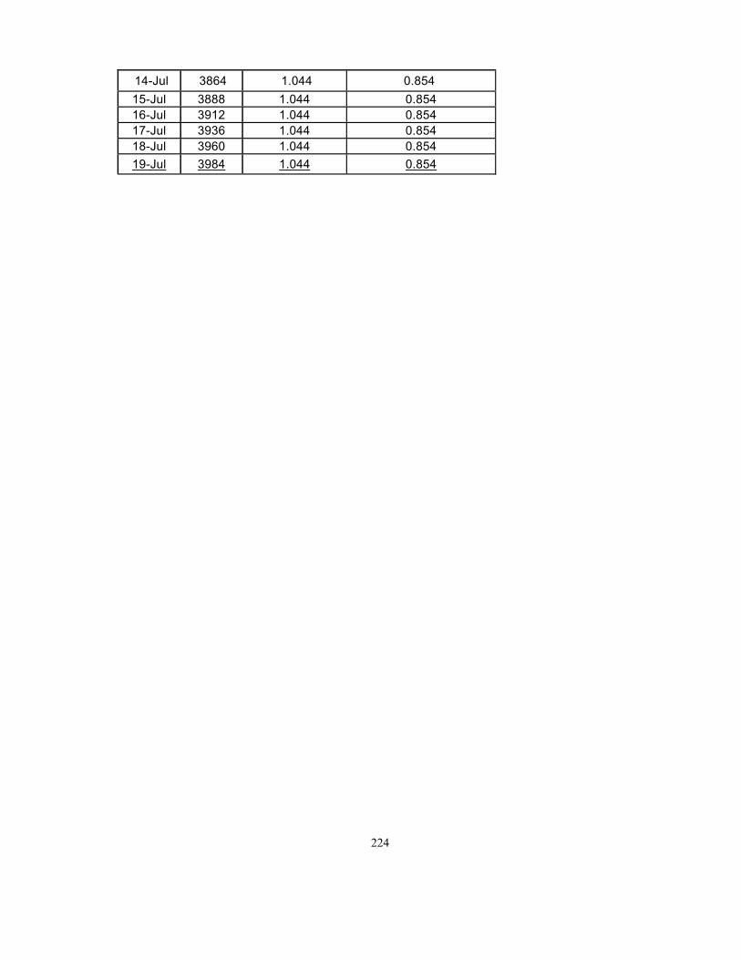
14-Jul 3864 1.044 0.854 15-Jul 3888 1.044 0.854 16-Jul 3912 1.044 0.854 17-Jul 3936 1.044 0.854 18-Jul 3960 1.044 0.854 19-Jul 3984 1.044 0.854

224

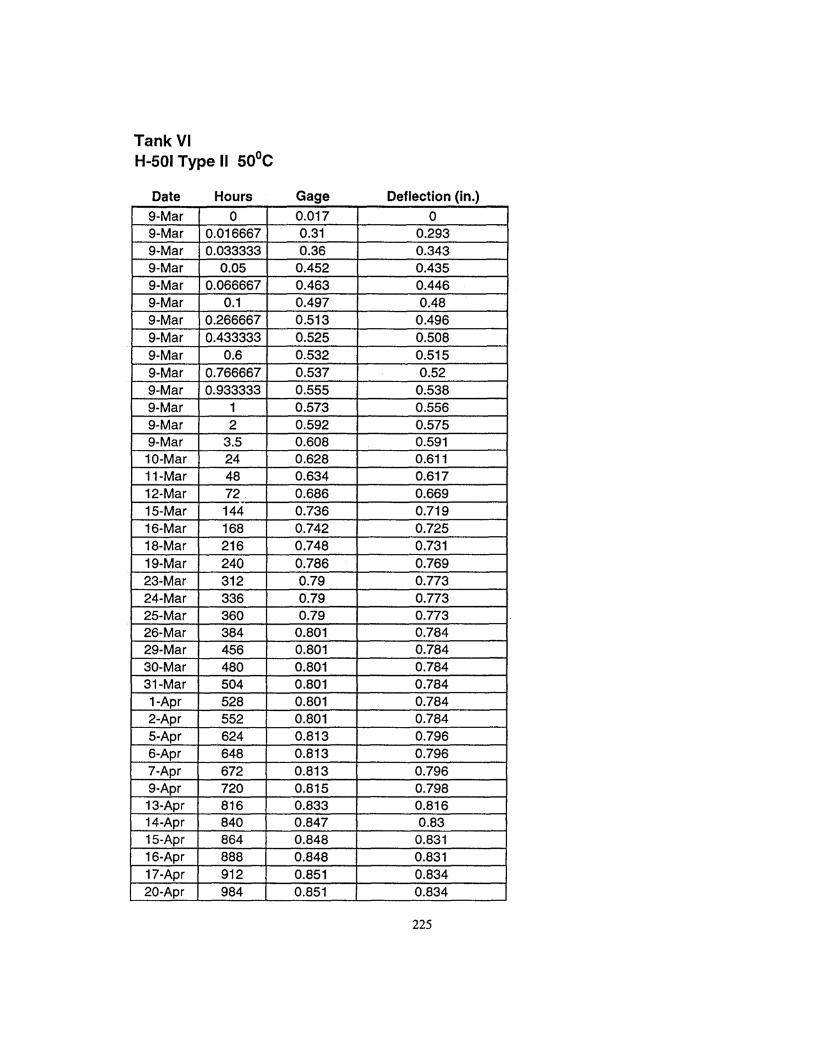
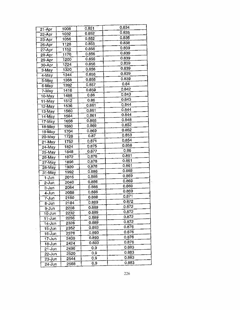
226

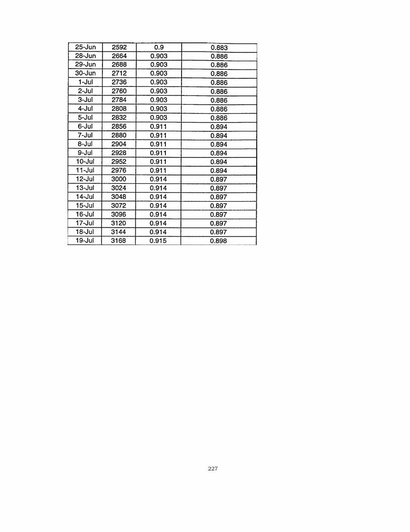
227

CHAPTER

9

DISCUSSI

ON

The discussion of the experimental and analytical findings is focused on certain

recent concerns, associated with the HDPE piping related to deflection, longitudinal, and

transverse stresses, long-term performance and service life prediction.

The characteristic length of the pipe, which is equal to the distance between the two

inflection points for a concentrated live loading for a pipe on Winkler foundation (equations

3.1, 3.2 and 3.3), was used for the length of the specimens. The CPPA (Corrugated

Polyethylene Pipe Association) and AASHTO (American Association of State Highway

Transportation Officials) both specify a minimum cover of one foot. Htruck loading was

of degradation. Oxidation reactions occur quite fast at super-ambient temperatures and

could lead to erroneous predictions of long-term properties of HDPE pipe specimens. In

view of the strong time and temperature dependence of polyethylene, application of super-

ambient temperatures alone (40°C and 50°C) was used to accelerate the failure mechanisms

for service life prediction of the viscoelastic HDPE pipe. A 7.5 % vertical change of diameter

(the failure criterion) or more was observed for the specimens heated at 50°C and under the

maximum loading.

As Aklonis and MacKnight [1983] pointed out, WLF time-temperature

superposition is not an effective methodology for the prediction of long-term behavior of

semi crystalline HDPE pipe [Ahn, 1999]. Therefore, life prediction, based on vertical

changes of diameter, was determined from the Arrhenius equation and the Bi-directional

Shifting Function Method. Both methods give similar life predictions but the BSM being

more conservative. For HDPE piping, the yield stress should not exceed 3,000 psi. Test results indicated that the maximum circumferential stress at the shoulder was approximately 436.82 psi, which is much less than the CPPA limit referred to above. The effective stress was even smaller (379.17 psi). It seems that the limit, which is based on yielding due to longitudinal bending, is not reasonable for the general failure criterion of the buried HDPE pipe subjected to live loading for the deflection 7.5% of the diameter.

The FEM software used (CANDE) has limitations for modeling of the corrugation and

valley without prismatic finite elements, and cannot take into account non-uniform

longitudinal soil properties and compaction. The creep was simulated from measurements

of the decrease of the flexural modulus as a function of time [Ahn, 1999]. 229

There is an agreement between experimental and CANDE deflections. The source of the error is that CANDE is two-dimensional software and surface loadings only can be defined as segmented uniform loads. CANDE cannot also take account of non-uniform longitudinal soil properties and compaction. The backfill modulus can vary along the pipe because the degree of saturation and the density of backfill soil change with time. For long-term service, it is difficult to ensure that the surrounding backfill environment will remain uniform along the pipe as in the installation stage. The backfill modulus can decrease if the degree of saturation increases. The backfill modulus can also vary along the pipe because of the degree of saturation and the density of backfill soil changing with time [Drumm et al., 1997]. Also, improper installation of the pipe and backfill soil can cause non-uniformity. Therefore, a need was identified to evaluate the long-term performance of the pipe, buried in non-uniform backfill conditions. This was addressed by an investigation of jointed pipes with the joints at the interfaces of two different soil media, simulating non-uniformity of the backfill (varying saturation and density). Investigation of the ring showed that the rates of modulus decay are quite similar for both Type I and II notched and un-notched specimens for long-term properties.

QA (Quality Assurance)/QC (Quality Control) conditions must be clearly specified for the

installation, maintenance and repair of the HDPE piping to reduce the problems

associated with non-uniform backfill conditions (for example ASTM D2321 Section S and

6, and AASHTO LRFD Design Specification Sections 12.4.1 and 12.6.2). 230

CONCLUSIONS The analytical and experimental investigation provided valuable information on the long-term behavior of buried HDPE pipes. Both circumferential and longitudinal bending was observed. A 7.5 % vertical change of diameter (the failure criterion), or more, was observed at approximately 3,200 hours for the specimens heated at 50°C, and subjected to maximum service loading. A 6% to 7% vertical change of diameter was observed at 10,000 hours for the specimens heated at 40°C and subjected to maximum service loading. Therefore, extrapolation for the vertical diametral change had to be made for the ambient, i.e. 20°C temperature, to determine the corresponding time of failure. From this, life prediction at ambient temperatures (20°C), corresponding to a 7.5% change in the vertical diameter, was made from the Arrhenius and the Bi-directional Methods. The maximum service lives for specimens at ambient temperature and subjected to maximum loading, were about 80 and 30 years for unnotched and notched specimens, respectively, assuming proper installation and a 90% compaction. Notches accelerated the vertical changes of diameter but no creep-rupture was observed within the time frame of 10,000 hours.

231

A supplementary investigation with notched and unnotched ring specimens,

exposed at the same temperatures, showed similar behavior of time transient deformation;

the behavior for Types I and II was also quite similar, ii) approximately after 3,500 hours,

both specimen Types I and II at 20°C became quite stable with few changes, while the

specimens at temperature over 20°C indicated changes in the deflection trend. The long-

term rates of modulus decay were also quite similar. But no cracking was found in all the

specimens during creep testing at super-ambient temperature levels.

CANDE 2-D analysis can be used to determine longitudinal bending, if several

cross-sectional locations are analyzed, and the deflections are used to define the

longitudinal profile with curve fitting. This analysis for 5,6001b loading gave a deflection

value of 0.20 in. compared to the experimental deflection of 0.194 in. at commencement

of testing the buried pipe. The approximations associated with CANDE analysis are its

restriction to two dimensions, and the specification of surface loading as segmented

uniform loading. CANDE cannot also take into account non-uniform longitudinal soil

properties and compaction. In the field, the backfill modulus can vary along the pipe

because of varying degrees of saturation and densities. Also, it is not possible to model the

corrugations.

The CPPA limit (3,000 psi), which is based on yielding due to circumferential bending, is not reasonable for the general failure criterion of the buried HDPE pipe subjected to live loading. The deflection threshold should be the governing failure criterion. Both experimental and numerical results clearly showed that longitudinal bending moments can occur in a jointed pipe, embedded in soil with varying properties; that are high enough to open the joints and cause leakage.

232

Hauser Laboratories, Boulder, CO, 1996.

244