www.concept.co.nz Long term gas supply and demand scenarios September 2014

Welcome message from author
This document is posted to help you gain knowledge. Please leave a comment to let me know what you think about it! Share it to your friends and learn new things together.
Transcript

www.concept.co.nz
Long term gas supply and demand scenarios
September 2014

About Concept
Concept Consulting Group Ltd (Concept) specialises in providing analysis and advice on energy-related issues. Since its formation in 1999, the firm’s personnel have advised clients in New Zealand, Australia, the wider Asia-Pacific region, and Europe. Clients have included energy users, regulators, energy suppliers, governments, and international agencies.
Concept has undertaken a wide range of assignments, providing advice on market design and development issues, forecasting services, technical evaluations, regulatory analysis, and expert evidence.
This report was prepared by Simon Coates, Bridget Moon and David Weaver.
Further information about Concept can be found at www.concept.co.nz.
Disclaimer
While Concept has used its best professional judgement in compiling this report, Concept and its staff shall not, and do not, accept any liability for errors or omissions in this report or for any consequences of reliance on its content, conclusions or any material, correspondence of any form or discussions, arising out of or associated with its preparation.
No part of this report may be published without prior written approval of Concept.
©Copyright 2014
Concept Consulting Group Limited
All rights reserved

Acknowledgement
The authors wish to thank the individuals and organisations that participated in interviews with staff from Concept and the Gas Industry Co as part of this project. The information provided by these organisations was extremely useful as a supplement to published data sources.

GAS SUPPLY AND DEMAND SCENARIOS 2014 - 2029 3
Executive summary .......................................................................................................................................5
Background and purpose of study ....................................................................................................5
Gas supply and market scenarios .....................................................................................................5
Annual demand projections ..............................................................................................................6
Peak demand projections .................................................................................................................8
1 Introduction ....................................................................................................................................... 10
Contrast with the 2012 study ........................................................................................................ 11
2 Gas supply and market scenarios ...................................................................................................... 12
2.1 Historical gas outcomes ............................................................................................................. 14
2.1.1 Introduction ....................................................................................................................... 14
2.1.2 Historical development of the New Zealand gas industry ................................................. 15
2.1.3 New Zealand’s gas consuming sectors ............................................................................... 22
2.1.4 Historical drivers of gas prices ........................................................................................... 25
2.1.5 Comparison of New Zealand's reserve to production ratios with other markets ............. 28
2.2 Future market scenarios ............................................................................................................ 29
2.2.1 Possible market states ....................................................................................................... 29
2.2.2 Near-term market outlook (< 5 years) ............................................................................... 31
2.2.3 Longer-term market outlook (5+ years)............................................................................. 33
2.2.4 Other gas supply issues ...................................................................................................... 34
The implications of deliverability and swing .................................................................................. 34
Non-Taranaki gas, and the risk of catching the ‘LNG disease’ ....................................................... 35
Reserves information ..................................................................................................................... 38
3 Gas demand scenarios – annual demand .......................................................................................... 41
3.1 Gas consuming sectors in New Zealand ..................................................................................... 43
3.2 Petrochemical ............................................................................................................................ 46
3.2.1 Methanol ............................................................................................................................ 46
Demand for gas for methanol production has varied significantly over time ............................... 46
Methanol production in New Zealand reflects the state of the global methanol market ............ 47
3.2.2 Urea .................................................................................................................................... 53
3.2.3 Summary petrochemical demand for different market scenarios .................................... 56
Comparison with 2012 study ......................................................................................................... 56
3.3 Power generation....................................................................................................................... 57
3.3.1 Gas for power generation internationally ......................................................................... 57
3.3.2 Gas for power generation in New Zealand ........................................................................ 57
Changes in demand ........................................................................................................................ 60
Changes in the relative economics of generation ......................................................................... 61
Combining demand, new renewables, and hydrology factors ...................................................... 62
3.3.3 Future demand growth ...................................................................................................... 67
Tiwai ............................................................................................................................................... 67

GAS SUPPLY AND DEMAND SCENARIOS 2014 - 2029 4
General electricity demand growth ............................................................................................... 68
3.3.4 The relative economics of coal, gas and renewables......................................................... 70
3.3.5 Summary gas for power generation projections ............................................................... 76
Results ............................................................................................................................................ 77
Discussion of results ....................................................................................................................... 81
Comparison with 2012 study ......................................................................................................... 82
3.4 Industrial, commercial and residential demand ........................................................................ 85
3.4.1 Historical movements in demand ...................................................................................... 85
3.4.2 Projections of gas demand from the industrial, commercial and residential sectors ....... 88
3.4.3 Comparison with 2012 study ............................................................................................. 92
3.5 Summary projections of gas demand ........................................................................................ 93
Hydrology uncertainty ................................................................................................................... 97
4 Gas demand scenarios – peak demand ............................................................................................. 99
4.1 Analysis of peak demand drivers ............................................................................................... 99
4.2 Projections of peak demand .................................................................................................... 107
Analysis of potential peak capacity issues for the Maui pipeline north of Mokau ...................... 110
Appendix A. Analysis on the extent to which electricity demand growth will be met by thermal versus renewable generation .............................................................................................................................. 113
The seasonal and diurnal variation in demand gives rise to a need for some generation to operate at low capacity factors ................................................................................................... 113
The characteristics of geothermal and wind plant make them not cost-effective options for meeting low capacity factor operation ........................................................................................ 114
Hydro stations with storage are the only renewables with the ability to cost-effectively meet the demand for low capacity factor operation – but their ability to provide more flexibility appears constrained .................................................................................................................................. 117
Estimation of the total residual demand for low capacity factor thermal generation, including performing hydro-firming duties ................................................................................................. 124
Appendix B. Description of the model used to develop power generation projections ..................... 127
Appendix C. 2012 analysis of relationship between demand and sectoral GDP and population ........ 130
Appendix D. Description of statistical model ....................................................................................... 135
Appendix E. Interruptibility .................................................................................................................. 148
Interruptibility from power generators ....................................................................................... 149
Interruption from other consumers ............................................................................................ 155

GAS SUPPLY AND DEMAND SCENARIOS 2014 - 2029 5
Executive summary
Background and purpose of study
Gas prices and demand in New Zealand have had a roller coaster ride over the past fifteen years. After enjoying relatively low prices and high gas demand at the start of the 2000’s, gas prices rose sharply in the first half of the last decade closely followed by a significant drop in gas demand. More recently, wholesale gas prices have fallen significantly and gas demand has once again started to rise.
This study analyses the main drivers for such historical outcomes, and the factors that are likely to drive future outcomes. The aim is to provide stakeholders with a broader understanding of the key issues, and thus to help them make better-informed decisions.
One aspect of this study is the development of possible market state scenarios for future gas supply and demand, and the prices that could emerge in such scenarios.
A model “Gas_Dem” has been developed to analyse historical demand patterns and undertake the demand projections for each of the gas market scenarios. It has been released in association with this report to help stakeholders get a better understanding of some of the demand drivers in New Zealand, and to enable them to do some of their own analysis.
This is the second Gas Supply and Demand study commissioned by Gas Industry Company. At the time the first study was undertaken in 2012, there was considerable industry interest as to whether certain parts of the Vector transmission system, particularly the North system, may face peak capacity constraints which would necessitate future investment. Accordingly, such peak capacity issues were a key focus of the 2012 study, which developed quantitative analysis to assess the issues.
In commissioning this second study, Gas Industry Company wanted additional focus on another key issue for the New Zealand gas sector: namely, the projected demand for gas for electricity generation, given this is the second largest source of gas demand and has seen significant changes in recent years. This 2014 study explores this issue in some detail, and considers the outlook for electricity demand, the impact of alternative renewable generation technologies, and other related issues.
Gas supply and market scenarios
Because New Zealand is not physically connected to any international gas markets (either by pipeline or LNG import / export facility), any gas that is discovered in New Zealand must be ‘consumed’ in New Zealand in order to be commercialised.
The ‘lumpy’ nature of new gas field discovery and production requires the ability for some gas users which can significantly increase – or decrease – demand to match the changing overall supply position.
The two sectors which have fulfilled this role in New Zealand are the power generation and petrochemical sectors – particularly Methanex’s two methanol production plants which have significantly varied their consumption to match the changing supply / demand position over the last 20+ years. The presence of this large source of flexible demand (Methanex gas demand is estimated to be ≈ 45% of projected total NZ demand for 2014) is considered to have been a key enabler of upstream exploration and production.
The uncertain and lumpy nature of gas discoveries means that New Zealand faces a range of possible futures. Three market scenarios have been developed to broadly reflect these possible futures:
1) Tight Supply – reflecting a situation where insufficient new gas is discovered / ‘proven-up’ to meet the rate of gas usage. Gas demand for methanol production will likely progressively decline which will help balance demand with supply. If insufficient gas is still not found methanol production will likely completely cease, and other gas consuming uses will start to reduce consumption – particularly gas for baseload power generation, urea production, and some industrial process heat. The end products from these various uses will be replaced, respectively by: other forms of power generation, imported urea, and alternative fuels for process heat (e.g. coal,

GAS SUPPLY AND DEMAND SCENARIOS 2014 - 2029 6
biomass, diesel). The opportunity cost of these other uses will likely set the price of gas as a particular end-use becomes the marginal source of demand. For example, if baseload power generation is the marginal source of gas demand, the equivalent gas netback for the cost of electricity produced by the next most cost-effective form of baseload generation (e.g. a new renewable station) will strongly influence gas prices.
2) Moderate Supply – reflecting a situation where gas is discovered / ‘proven-up’ at a rate which more or less matches demand over time. Methanol production is likely to act as the main ‘balancing’ source of demand to match supply, provided a sizeable proportion of the existing methanol plant capacity in Taranaki is available for operation. This means that prices will likely be strongly influenced by the economics of producing methanol in New Zealand versus other international locations. For the next 10-15 years this marginal source of international methanol supply appears likely to be North America. Such methanol-linked prices are currently predominating in New Zealand, with wholesale prices being around $6/GJ.
3) Plentiful Supply – reflecting a situation where new, low cost gas resources become available and the volume of supply significantly exceeds the demand of existing gas consumers. Prices would fall to a level that stimulates additional demand. In the limit, the floor for this scenario is likely to be the price that new gas consuming petrochemical facilities would be willing to pay.
In recent years, New Zealand’s gas market has been experiencing conditions along the lines of the Moderate Supply scenario, with a broad balance between supply and demand and gas prices strongly influenced by the economics of methanol production. Based on present information, the most likely outcome appears to be a continuation of similar types of conditions for the next five years or so, although potentially with some downward price pressures in the earlier part of the period.
As we look further into the future, there is more uncertainty about potential outcomes because a greater range of factors can come into play. Notwithstanding this observation, of the three market scenarios, Moderate Supply appears to be the most likely outcome over time. This is because there are natural balancing forces that are expected to bring the market back toward equilibrium if the New Zealand gas market moves into a position of relative scarcity (i.e. the tight scenario) or surplus (i.e. the plentiful scenario).
This is consistent with how the reserves to production ratios (RTPs) 1 in other countries also vary from year to year based on exploration success, but tend to converge to similar levels (RTPs of roughly 10 to 15 years) over time. Given that the economics of monetising gas via power generation, petrochemicals or LNG are fundamentally similar around the world, such convergence of RTP ratios is not surprising.
Given this dynamic, prices over the long-term will likely tend towards those consistent with the Moderate Supply scenario – i.e. with prices strongly influenced by the economics of producing methanol in New Zealand versus other international locations.
Annual demand projections
Gas demand can be split into three main segments: 1) petrochemical; 2) power generation; 3) direct use of gas to provide energy for the industrial, commercial and residential sectors
1 The reserves to production ratio is a measure of how many years’ worth of gas exists to meet existing demand.

GAS SUPPLY AND DEMAND SCENARIOS 2014 - 2029 7
Gas demand for petrochemicals is likely to continue to be dominated by Methanex’s two production facilities at Motunui and Waitara Valley. During periods of Plentiful Supply these are likely to operate at full capacity (currently 90PJ/y), whereas in periods of Tight Supply they are likely to be mothballed. The figure on the right shows how this has been played out over the past fifteen years as New Zealand’s reserves position has changed.
The other main petrochemical gas consumer – Ballance’s urea production facility at Kapuni – is likely to continue at current levels (≈7PJ/yr) for the next decade or so.2 Only if a sustained Tight Supply scenario were to emerge would it be likely to exit, but would probably do so later than Methanex.3 Conversely, in a sustained Plentiful Supply scenario, it is more likely that additional investment would occur in new urea production facility than a new methanol production facility.
This difference in price sensitivity for urea versus methanol production is because New Zealand is a net importer of urea, whereas almost all the methanol produced in New Zealand is exported. As such the avoided shipping costs materially affect urea and methanol’s relative economics.
Hydrology-corrected4 gas demand for thermal power generation has fallen considerably from a peak of 90 PJ in 2001 to 55 PJ in 2013. This has been due to a decline in electricity demand and the ‘premature’-build of significant amounts of new renewable generation.5 These two factors are likely to continue to result in further decline out to 2017. Gas demand for power generation is likely to increase again beyond 2017, although could fall further in some scenarios associated with the complete exit of the Tiwai aluminium smelter.
Scenarios of projected gas demand for power generation in 2025 ranges from 100 PJ/yr down to 20 PJ/yr. In descending order of priority, the key factors driving these different outcomes are:
2 It is possible that investment in modernising the existing plant to achieve improved gas conversion efficiencies may marginally increase the amount of gas consumed by the Kapuni plant (e.g. by the order of 1-2 PJ/yr) – even if it substantially increases the output of urea. 3 This assumes that the existing petrochemical plant in Taranaki remains in service, and does not require any major capital expenditure to maintain safe and reliable operation. 4 A significant amount of year-to-year variation in thermal generation is due to variation in hydro output. ‘Hydrology-corrected’ analysis is based on what hydro output would have been if inflows were at mean levels observed historically. 5 The new renewable generation has been classed as ‘premature’ as both electricity demand growth and fossil & CO2 prices have turned out to be a lot lower than were the expectations at the time the renewable plant were committed.

GAS SUPPLY AND DEMAND SCENARIOS 2014 - 2029 8
Future electricity demand growth / decline – particularly for the Tiwai aluminium smelter.
Whether or when the current multi-year ‘dry’ phase of hydrology (which started in 2000) reverts back to mean hydrology levels or even to a ‘wet’ phase.
Future CO2 prices, which are key in determining the extent to which gas-fired generation is competitive with Huntly power station burning coal
Future gas prices. In combination with CO2 prices, these will be key determinants of the extent to which future electricity demand growth is met by increasing the utilisation of existing gas-fired power generators, or by building new renewables.
Any retirement or re-configuration of existing thermal plant – particularly Contact’s and MRP’s CCGTs, and further Huntly coal units6
The future cost of new renewables – which in turn is strongly driven by NZ$ exchange rates
The rate of change of gas demand for the direct use of gas for energy is projected to be relatively modest, ranging between average annual growth of 1.8% for the plentiful supply scenario, and -0.75% for the tight supply scenario. This is due to:
The rates of change of the key drivers for energy services (population and GDP growth) being themselves relatively modest; and
Opportunities for economic fuel switching tending to be dominated by capital replacement decisions. Given the long lifetimes of boilers and space & water heaters, this results in low capital replacement rates
Taken together across all three demand segments, the inherently wide range of uncertainty for key drivers gives rise to a wide range of possible long-term gas demands.
Peak demand projections
When considering the implications of future demand on pipeline investments it is necessary to project peak demands, not annual demands. For some pipelines peak-day demand is critical, whereas for others it is the peak-week demand – with the difference being due to how much line pack each pipeline has available.
Different demand segments make different contributions to system peak demands due to different seasonal consumption patterns, and different weather sensitivities (i.e. demand being linked to outside
6 Genesis has already retired or put into storage two of its four Huntly units

GAS SUPPLY AND DEMAND SCENARIOS 2014 - 2029 9
temperature). The two segments which have the greatest weather-sensitivity and seasonal consumption patterns are the Non-ToU (i.e. mass-market) segment, and power generation.
The apparent drop in peak demand from 2011 for many pipeline regions is largely due to weather in subsequent years not being as severe as during the August 2011 extreme weather event. On a weather-corrected basis, the peak demands across the years are much more similar.
One option for addressing peak demand is to temporarily interrupt some demand segments. Historically, the Marsden Point refinery is the only material load which has been on an interruptible contract. However, a significant un-tapped potential exists from the power generation sector and some industrial process heat demands that would be much cheaper than investing in upgrading pipeline capacity.
The two pipeline systems which have received greatest focus on the potential future need to upgrade pipeline capacity are the Vector North system, and the Mokau compressor serving all Maui pipeline load north of this point. Study projections indicate that it is extremely unlikely such capacity upgrades will be required, particularly due to:
The potential for interruption from power generation and some industrial process heat loads;
The possibility that the Otahuhu B CCGT power station could be re-configured to OCGT mode.

GAS SUPPLY AND DEMAND SCENARIOS 2014 - 2029 10
1 Introduction
As is indicated by Figure 1 below, natural gas7 prices and demand in New Zealand have had a roller coaster ride over the past fifteen years. After enjoying relatively low prices and high gas demand at the start of the 2000’s, gas prices rose sharply in the first half of the last decade closely followed by a significant drop in gas demand. More recently, wholesale gas prices have fallen significantly and gas demand has once again started to rise.
Figure 1: Historical New Zealand gas demand and industrial gas prices8
Source: Concept analysis using MBIE data
This study analyses what have been the main drivers for outcomes over the past fifteen years, and key factors that are likely to drive future outcomes over the next fifteen years. The aim is to provide stakeholders with a broader understanding of the key issues, and thus to help them make better-informed decisions.
The structure of the study is as follows:
Section 2 analyses the factors driving upstream gas supply, and sets out the scenarios for possible future gas prices
Section 3 analyses the factors driving downstream gas demand, and develops projections of gas demand for the gas market scenarios
Section 4 analyses the factors driving peak demand , and develops projections of peak demand for different parts of the network for the different gas market scenarios
7 Henceforth, references to ‘gas’ means natural gas, unless otherwise stated. 8 There is limited public information on gas prices in New Zealand. One of the few sources is data on gas prices paid by for large industrial consumers, excluding petrochemical consumers. This data covers around 12% of total gas demand, but provides a barometer for the wider gas market. The data includes charges for transmission and distribution network – considered to be approximately $1-2/GJ of this total.

GAS SUPPLY AND DEMAND SCENARIOS 2014 - 2029 11
One aspect of this study is the development of possible market state scenarios for future gas supply and demand, and the prices that could emerge in such scenarios.
A model “Gas_Dem” has been developed to analyse historical demand patterns and undertake the demand projections for each of the gas market scenarios. It has been released to the public in association with this report to help stakeholders get a better understanding of some of the demand drivers in New Zealand, and to enable them to do some of their own analysis. It can be downloaded from the Gas Industry Co website at the same location that this report is published.
Contrast with the 2012 study
This is the second Gas Supply and Demand study commissioned by Gas Industry Company. At the time the first study was undertaken in 2012, there was considerable industry interest as to whether certain parts of the Vector transmission system, particularly the North system, may face peak capacity constraints which would necessitate future investment. Accordingly, such peak capacity issues were a key focus of the 2012 study, which developed quantitative analysis to assess the issues.
In commissioning this second study, Gas Industry Company wanted additional focus on another key issue for the New Zealand gas sector: namely, the projected demand for gas for electricity generation, given this is the second largest source of gas demand and has seen significant changes in recent years. This 2014 study explores this issue in some detail, and considers the outlook for electricity demand, the impact of alternative renewable generation technologies, and other related issues.

GAS SUPPLY AND DEMAND SCENARIOS 2014 - 2029 12
2 Gas supply and market scenarios
Chapter summary
Because New Zealand is not physically connected to any international gas markets (either by pipeline or LNG import / export facility), any gas that is discovered in New Zealand must be consumed in New Zealand in order to be commercialised.
The ‘lumpy’ nature of new gas field discovery and production requires the ability for some gas consuming uses which can significantly increase – or decrease – demand to match the changing supply position
The two sectors which have fulfilled this role in New Zealand are the power generation and petrochemical sectors – particularly Methanex’s two methanol production plants which have significantly varied their consumption to match the changing supply / demand position over the last 20+ years. The presence of this large source of flexible demand (Methanex gas demand is estimated to be ≈ 45% of projected total NZ demand for 2014) is considered to be a key enabler of upstream exploration and production.
The uncertain and lumpy nature of gas discoveries means that New Zealand faces a range of possible futures. Three market scenarios have been developed to broadly reflect these possible futures:
1) Tight Supply – reflecting a situation where insufficient new gas is discovered / ‘proven-up’ to meet the rate of gas usage. Gas demand for methanol production will likely progressively decline which will help balance demand with supply. If insufficient gas is still not found methanol production will likely completely cease, and other gas consuming uses will start to reduce consumption – particularly gas for baseload power generation, urea production, and some industrial process heat. The end products from these various uses will be replaced, respectively by: other forms of power generation (e.g. renewables), imported urea, and alternative fuels for process heat (e.g. coal, biomass, diesel). The opportunity cost of these other uses will likely set the price of gas as a particular end-use becomes the marginal source of demand. For example, if baseload power generation is the marginal source of gas demand, the equivalent gas netback for the cost of electricity produced by the next most cost-effective form of baseload generation (e.g. a new renewable station) will strongly influence gas prices.
2) Moderate Supply – reflecting a situation where gas is discovered / ‘proven-up’ at a rate which more or less matches demand over time. Methanol production is likely to act as the main ‘balancing’ source of demand to match supply, provided a sizeable proportion of the existing methanol plant capacity in Taranaki is available for operation. This means that prices will likely be strongly influenced by the economics of producing methanol in New Zealand versus other international locations. For the next 10-15 years this marginal source of international methanol supply appears likely to be North America. Such methanol-linked prices are currently predominating in New Zealand, with wholesale prices being around $6/GJ.
3) Plentiful Supply – reflecting a situation where new, low cost gas resources become available and the volume of supply significantly exceeds the demand of existing gas consumers. Prices would fall to a level that stimulates additional demand. Low prices from this plentiful scenario would be unlikely to persist, as the additional demand that would be stimulated would act to bring the market back into balance, with prices returning over time to those consistent with the Moderate Supply scenario.
In recent years, New Zealand’s gas market has been experiencing conditions along the lines of the Moderate Supply scenario, with a broad balance between supply and demand and gas prices strongly influenced by the economics of methanol production. Based on present information, the most likely outcome appears to be a continuation of similar types of conditions for the next five years or so, although potentially with some downward price pressures in the earlier part of the period.

GAS SUPPLY AND DEMAND SCENARIOS 2014 - 2029 13
As we look further into the future, there is more uncertainty about potential outcomes because a greater range of factors can come into play. Notwithstanding this observation, of the three market scenarios, Moderate Supply appears to be the most likely outcome over time. This is because there are natural balancing forces that are expected to bring the market back toward equilibrium.
This is consistent with how the reserves to production ratios (RTPs) 9 in other countries also vary based on exploration success, but tend to converge to similar levels (RTPs of roughly 10 to 15 years) over time. Given that the economics of monetising gas via power generation, methanol or LNG are fundamentally similar around the world, such convergence of RTP ratios is not surprising.
Given this dynamic, prices over the long-term will likely tend towards those consistent with the Moderate Supply scenario – i.e. with prices strongly influenced by the economics of producing methanol in New Zealand versus other international locations.
9 The reserves to production ratio is a measure of how many years’ worth of gas exists to meet existing demand.

GAS SUPPLY AND DEMAND SCENARIOS 2014 - 2029 14
2.1 Historical gas outcomes
2.1.1 Introduction
Gas in New Zealand is currently produced entirely in the Taranaki region. Figure 2 below shows where these various gas (and oil) fields are located.
Figure 2: Map of New Zealand's current oil and gas fields
Source: “Energy in New Zealand 2013”, MBIE
This Taranaki-produced gas is reticulated in the North Island via a transmission network that links most of the main population centres. This transmission network is shown in Figure 3 below.

GAS SUPPLY AND DEMAND SCENARIOS 2014 - 2029 15
Figure 3: Map of New Zealand's gas transmission network
Currently there is no natural gas reticulated in the South Island.
2.1.2 Historical development of the New Zealand gas industry
New Zealand’s gas industry started in the early 1970s with the discovery and development of the onshore Kapuni field in Taranaki. A few years later, the Maui gas field was discovered in offshore Taranaki.

GAS SUPPLY AND DEMAND SCENARIOS 2014 - 2029 16
When it was discovered the Maui field was large by world standards. As Figure 4 below shows, production from the Maui field dominated the New Zealand gas sector for the following two and a half decades.
Figure 4: Historical gas production in New Zealand
Source: Concept analysis using MBIE data
The Taranaki basin is generally thought to have good prospects for more oil and gas fields to be discovered. However, as Figure 4 illustrates, for roughly twenty years there was no further development of significant new gas fields. Major development only began once the Maui field started going into decline. The Pohokura and Kupe fields have been particularly significant in replacing the declining Maui gas production.
That is not to say there was no hydrocarbons exploration and development in New Zealand during the 1980’s and 1990’s. As Figure 5 below shows, the McKee and Waihapa fields were developed in the 1980s. However, these are / were predominantly oil producing fields, with relatively little gas being produced. More recently, the offshore Maari and Tui fields have been developed, with these fields producing only oil.

GAS SUPPLY AND DEMAND SCENARIOS 2014 - 2029 17
Figure 5: Historical oil production in New Zealand
Source: Concept analysis using MBIE data
To understand this apparent relative lack of gas exploration effort in the decades following Maui’s development, and the difference with oil exploration and production, it is necessary to understand an important feature of the New Zealand gas sector – namely that it is not physically connected to other gas markets.
This is relatively unusual for a western economy, with Iceland being the only other OECD country without a physical ability to transport gas to / from other gas markets. All other OECD economies are connected to other gas markets: either through pipelines, or through having liquefied natural gas (LNG) import or export capabilities.10
The implication of this is that any gas that is produced in New Zealand must be consumed within New Zealand. This also contrasts with oil production in New Zealand given that it is relatively straightforward to export oil to international markets via ship. This difference between New Zealand’s gas and oil sectors is illustrated in Figure 6 below.
10 LNG is transported between countries via ship.

GAS SUPPLY AND DEMAND SCENARIOS 2014 - 2029 18
Figure 6: Historical gas and oil production and consumption11
Source: Concept analysis using MBIE data
The production and consumption of gas in New Zealand is almost exactly equal12, whereas there is a huge difference between indigenous oil production and domestic oil consumption.
Indeed, as Figure 7 below illustrates, almost all oil produced in New Zealand is exported, with New Zealand’s domestic oil consumption being almost entirely met through importing oil from overseas (being a mixture of unrefined oil which is then processed in the Marsden Point refinery, and already refined oil products (i.e. diesel, petrol, aviation fuel etc.)).
11 Data on domestic gas consumption from a number of sectors is not available prior to 1990. 12 Much of the differences is understood to be due to statistical measurement & reporting issues.

GAS SUPPLY AND DEMAND SCENARIOS 2014 - 2029 19
Figure 7: Historical production, consumption, imports and exports of oil13
Source: Concept analysis using MBIE data
The fact that any gas produced in New Zealand must be consumed in New Zealand has implications for the economics of exploration and production in New Zealand. In particular, an upstream producer must have confidence that it can commercialise any gas that is found through selling to New Zealand-based gas consumers.
This is not just an issue for gas exploration, but also for oil exploration and production given that for many New Zealand fields, gas and oil are found and produced together. This can be seen by looking back at Figure 4 and Figure 5 and comparing the historical pattern of gas and oil production for a number of the fields– e.g. the historical pattern of production at the Maui, Kapuni and Pohokura fields has been very similar between oil and gas.
The extent to which gas and oil are found at the same fields is further illustrated in Figure 8 below which shows the proportion of oil and gas for ultimately recoverable reserves for nine of New Zealand’s largest fields.
13 For the purposes of this illustration the ‘consumption’ line has been derived as being equal to: Production + Imports – Exports. In reality consumption is more complicated as there can be material year-to-year stock changes, and the need to account for aspects such as fuel consumed by international transport (ships + planes)

GAS SUPPLY AND DEMAND SCENARIOS 2014 - 2029 20
Figure 8: Estimated P50 probability ultimately economically recoverable oil and gas reserves as at 1 January 2014 (PJ)
Source: Concept analysis using MBIE data
Figure 9 below shows the same data but on a proportional basis, plus including an estimate of the proportion of the relative value of the gas and oil for a given assumption about oil and gas prices.

GAS SUPPLY AND DEMAND SCENARIOS 2014 - 2029 21
Figure 9: Proportional split between oil and gas reserves and value for main New Zealand fields as at 1 January 2014
Source: Concept analysis using MBIE data
Due to the time value of money (i.e. a million dollars earned now is of higher value than a million dollars earned in the future) an upstream producer will want to extract and produce any oil and gas as quickly as possible – all other things being equal. However, to produce hydrocarbons more quickly generally requires greater investment, for example in more production wells or downstream processing facilities.
Determining the value-maximising amount to invest involves complex trade-offs between being able to produce oil & gas more quickly versus the extra capital investment required to do so – noting that the specific geology of the field will also have a significant bearing on how quickly oil and gas can be extracted. The results of this value equation mean that it may be most economic to extract oil & gas from some fields ‘slowly’ over many decades (and size the production facilities to be smaller), whereas for other fields it may be most economic to extract the hydrocarbons ‘quickly’ over a much shorter period of time and invest in larger in-field and production capabilities.
This can be seen by looking at the oil production profiles shown previously in Figure 5. The Kapuni field is an example of where production has occurred over many decades, whereas Waihapa is an example of a field where the main production occurred over the space of a single decade.
This value equation governing production investment occurs for all oil and gas fields around the world. However in New Zealand, the fact that gas produced locally must be consumed locally adds another dimension to this equation. In the scenario of a major gas find, the sizing of the production capabilities may be constrained by the size of the local demand to take the gas.
As Figure 9 illustrates, the extent to which any gas that is found can be commercialised can have a significant bearing on the economics of exploration and production, even if the greatest proportion of value comes from the oil.
The challenge for gas producers is that it is not possible to ‘manufacture’ gas demand from thin air. There needs to be an economic use for the gas.

GAS SUPPLY AND DEMAND SCENARIOS 2014 - 2029 22
A related challenge is that the production profiles of oil and gas fields can be quite steep initially, with fields having the potential for significant rates of production when they first come on line. For example, as Figure 10 below illustrates, the Maui, Pohokura, and Kupe fields all went from zero production to full output in a relatively short space of time.
Figure 10: Historical gas production from New Zealand's main gas fields
Source: Concept analysis using MBIE data
2.1.3 New Zealand’s gas consuming sectors
This challenge of commercialising large amounts of gas in a relatively short space of time is virtually impossible to meet solely from selling gas to be used for direct use as an energy fuel.14 As set out further in section 3.4, this is because growth in the demand for such energy is primarily driven by GDP and population growth (which is generally of the order of a couple of percent per year), and the economics of fuel switching to gas away from other fuels being used to provide such energy services (e.g. coal or diesel) are dominated by the capital replacement costs associated with switching. Accordingly, growth in the demand for gas for direct use to provide energy is relatively slow, and couldn’t generally accommodate the significant increase in output that has been seen historically as a major new field comes on line.
Using gas for power generation has been a more feasible approach to rapidly increasing gas consumption to commercialise a gas find. Following the discovery of the Kapuni and Maui fields, plans for two of New Zealand’s biggest power stations (New Plymouth and Huntly) were reconfigured to allow for the burning of gas as the primary fuel (rather than fuel oil or coal). More recently, four combined cycle plants were developed to burn gas in the 1990’s and 2000’s. However, as section 3.3 sets out, there may be more constraints on the ability to commercialise large quantities of gas via power generation in New Zealand in the future.
14 Such direct use for energy is principally to meet three main requirements: to raise process heat for industrial and commercial customers, and for space and water heating for residential and commercial customers.

GAS SUPPLY AND DEMAND SCENARIOS 2014 - 2029 23
The last main option to commercialise significant quantities of gas is to convert it into a petrochemical product. In New Zealand significant quantities of gas have been commercialised this way with the development of two methanol production plants, the Kapuni fertiliser plant, and a (now retired) synfuel15 production plant.
As Figure 11 and Figure 12 below illustrate, these three different sectors (direct use of gas for energy, power generation, and petrochemical) have played very different roles in commercialising gas in New Zealand:
Figure 11: Historical gas consumption in New Zealand – area graph
Source: Concept analysis using MBIE data
15 Synfuel is a petrol substitute.

GAS SUPPLY AND DEMAND SCENARIOS 2014 - 2029 24
Figure 12: Historical gas consumption in New Zealand – line graph
Source: Concept analysis using MBIE data
To be a good enabler for the upstream industry, a consuming sector needs some ability to increase consumption at times when a new gas field comes on stream, but it also means having some ability to decrease consumption at times when gas production reduces as a field becomes depleted.
Looking at the above graphs:
Direct use of gas has been very stable on a year-to-year basis, and thus not facilitated the rapid increase (and sometimes decrease) in production from gas fields;
Power generation has been able to increase (and decrease) consumption to match changing gas production positions to a significant extent
Petrochemical production has been the sector that has been most able to vary consumption to match changing gas production positions.
In summary, the petrochemical and power generation sectors have been the most important enablers of gas and oil production in New Zealand, with the petrochemical sector exhibiting the greatest flexibility.

GAS SUPPLY AND DEMAND SCENARIOS 2014 - 2029 25
2.1.4 Historical drivers of gas prices
This section discusses how New Zealand’s changing gas position has influenced gas prices.
Figure 13 below shows how total estimated remaining reserves in New Zealand dropped significantly in 2001 due to the re-determination of remaining reserves in the Maui field.
Figure 13: Annual change in P50 reserves (LHS) and total reserves (RHS)
Source: Concept analysis using MBIE data

GAS SUPPLY AND DEMAND SCENARIOS 2014 - 2029 26
Figure 14 below shows how gas consumption dropped significantly in 2003 and 2004 in response to reduced reserves – with the change borne principally within the petrochemical sector (as has previously been shown in Figure 12 on page 24).
Figure 14: Historical change in remaining P50 reserves and annual consumption
Source: Concept analysis using MBIE data
This major drop in consumption helped reduce the rate of decline of gas reserves, with annual demand being brought closer to the levels of new reserves being ‘proven’ in existing fields.16
As illustrated in Figure 13 above, gas reserves only increased to previous levels with the bringing on stream of two major new fields – Pohokura and Kupe.
Another way in which the relative scarcity of gas is measured is to calculate the reserves to production ratio. As the name suggests, this is simply the ratio of proven remaining reserves to annual production.
The change in reserve to production ratios over the last 15 years is shown in Figure 15 below, along with average gas prices for industrial consumers (excluding power generation and petrochemical consumers). These customers only account for around 10% of gas use, and the average prices paid by other sectors can differ from that paid by industrial users (for example to reflect differences in pipeline charges and contract terms). Despite these caveats, the industrial customer price data is useful because it is the only data that is published on a regular and reasonably consistent basis. It therefore provides a general barometer of overall trends in average wholesale gas prices.
16 This proving of ‘new’ reserves refers to contingent resources in existing fields which were proven up via additional drilling or other work to allow them to be classified as probable reserves.

GAS SUPPLY AND DEMAND SCENARIOS 2014 - 2029 27
Figure 15: Historical P50 reserve: production ratios and gas prices to industrial consumers17
Source: Concept analysis using MBIE data
As gas started to become scarce (denoted by a fall in the reserve to production ratio), average prices paid by industrial consumers started to rise. Then as gas reserves became more plentiful again in the late 2000’s, average prices started to fall again before levelling off.18
During the early 2000’s as the level of reserves dropped to a point where the levels of consumption seen in the 1990s couldn’t be sustained, Methanex progressively scaled back its production (as indicated by the dropping of petrochemical demand in Figure 12 shown previously). During this period wholesale prices appeared to be strongly influenced by the willingness to pay from the power generation sector. These prices were relatively high in the short-term given the strong driver to find fuel for the recently developed gas-fired plant. In the longer-term, the price benchmark was driven by the main competing forms of generation – being new renewables for baseload power for CCGTs, and Huntly on coal for mid-merit and peaking power.
During this period the wholesale price of gas rose to levels approaching $9-10/GJ. However, as the reserves position started to change in the late 2000’s with the bringing on of Pohokura and Kupe, the amount of gas available started to exceed the demand from the direct use for energy and power generation sectors – particularly, as is set out in more detail in section 3.3, as the demand for power generation started to decline due to a fall in electricity demand and displacement by new renewables.
17 Prices for industrial consumers include transport (i.e. pipeline network) costs. These are not known, but estimated to be approximately $1-2/GJ depending on usage characteristics and whether the industrial consumer is connected to the transmission or distribution network. 18 There appears to be a lag in prices responding to the change in reserves. This is likely to be because the data series represents the price paid by industrial consumers in a given year, and many industrial consumers purchase their gas on multi-year contracts. Thus, in 2002, many industrial consumers would be paying for gas via long-term contracts struck several years previously. The prices in these longer-term contracts would likely be significantly lower than the prices being struck in contracts struck in 2002 when the reserves situation was more scarce.

GAS SUPPLY AND DEMAND SCENARIOS 2014 - 2029 28
This situation led to increased gas sales to Methanex, who started to bring more of their plant back into production. With Methanex effectively being the marginal consumer during this most recent period, wholesale gas prices have been strongly influenced by Methanex’s willingness to pay. This in turn is governed by the netback available from methanol production (which acts as a cap) and the cost of gas at other locations where Methanex has spare production capacity (which sets the floor).19 These issues are set out in more detail in section 3.2.1.
2.1.5 Comparison of New Zealand's reserve to production ratios with other markets
Some commentators have suggested that having only ten years’ worth of gas (as indicated by the reserves to production ratio) is too low. However, comparison of international data indicates that such outcomes are fairly typical by world standards. This is illustrated in Figure 16 and Figure 17.
The tendency for reserves to production ratios to converge at around 10-15 years occurs because there are some natural balancing influences that affect the ratio.
Figure 16: Reserves (P50) to production ratio and remaining reserves
Source: BP Statistical Review, Ministry of Business, Innovation and Employment, Energy Data Files.
In essence, countries or regions where large gas reserves are found tend to develop new gas-using industries, particularly export of gas via pipelines or as liquefied natural gas or methanol20, as well as domestic major uses of gas such as power generation. This is shown by the steeply falling ratio for Norway and Mexico in Figure 17 below. As the LNG production facilities in Australia start to come on line, the reserves to production ratio for this country will also sharply decline.
Conversely, if gas reserves decline in a country or region, gas export and ‘discretionary’ gas uses such as gas-fired power generation will tend to throttle back.
The other feedback loop is that the presence of viable outlets for gas will encourage the investment needed to commercialise contingent gas resources, and convert them to ‘proven’ reserves. For
19 Noting that prices would also need to reflect differences in relative transport costs to market for methanol, plant efficiency differences, emissions charge regimes etc. 20 Or more generally, as so-called gas-to-liquids products.

GAS SUPPLY AND DEMAND SCENARIOS 2014 - 2029 29
example, this is evident in Eastern Australia where coal seam gas resources have been recognised for many years, but the investment to convert them to reserves was only undertaken when a market was secured via LNG sales contracts. This also occurred for the development of the Kupe field in New Zealand which was discovered in 1986, but wasn’t developed until the late 2000’s.
Figure 17: International comparison of reserves to production ratios
Source: Concept analysis using BP Statistical Review data
Given that the economics of monetising gas via power generation, methanol or LNG are fundamentally similar around the world, it is not surprising that RTP ratios tend to converge over time.
2.2 Future market scenarios
This section describes a range of possible scenarios for the overall state of the gas market. These scenarios are used later in this report to inform the development of sector specific projections for gas demand.
The scenarios are not forecasts per se, but rather provide indications of possible futures under the specific scenario assumptions. They also assume that all other factors outside the scenario variables remain the same (e.g. oil prices remain around current levels, technology is relatively stable).
2.2.1 Possible market states
While there is a continuum of possible gas market states, it is useful to consider three key market scenarios: Tight Supply, Moderate Supply, and Plentiful Supply. These states are useful because they define the possible ‘book ends’, and a ‘middle’ zone.
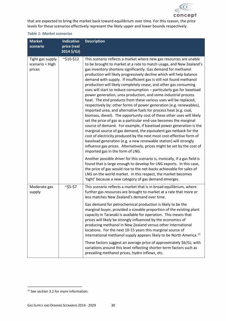
Table 1 describes each market scenario and the demand-side or supply-side factors that could cause it to arise. The table also describes the key drivers that would be expected to influence prices in each scenario.
It is important to note that the indicative prices for the Tight and Plentiful Supply scenarios reflect expected levels if the relevant market conditions were to persist over a sustained period. As discussed later in this report, such outcomes appear relatively unlikely because there are natural balancing forces
GAS SUPPLY AND DEMAND SCENARIOS 2014 - 2029 30
that are expected to bring the market back toward equilibrium over time. For this reason, the price levels for these scenarios effectively represent the likely upper and lower bounds respectively.
Table 1: Market scenarios
Market scenario
Indicative price (real 2014 $/GJ)
Description
Tight gas supply scenario = High prices
~$10-$12 This scenario reflects a market where new gas resources are unable to be brought to market at a rate to match usage, and New Zealand’s gas inventory shortens significantly. Gas demand for methanol production will likely progressively decline which will help balance demand with supply. If insufficient gas is still not found methanol production will likely completely cease, and other gas consuming uses will start to reduce consumption – particularly gas for baseload power generation, urea production, and some industrial process heat. The end products from these various uses will be replaced, respectively by: other forms of power generation (e.g. renewables), imported urea, and alternative fuels for process heat (e.g. coal, biomass, diesel). The opportunity cost of these other uses will likely set the price of gas as a particular end-use becomes the marginal source of demand. For example, if baseload power generation is the marginal source of gas demand, the equivalent gas netback for the cost of electricity produced by the next most cost-effective form of baseload generation (e.g. a new renewable station) will strongly influence gas prices. Alternatively, prices might be set by the cost of imported gas in the form of LNG.
Another possible driver for this scenario is, ironically, if a gas field is found that is large enough to develop for LNG exports. In this case, the price of gas would rise to the net-backs achievable for sales of LNG on the world market. In this respect, the market becomes ‘tight’ because a new category of gas demand emerges.
Moderate gas supply
~$5-$7
This scenario reflects a market that is in broad equilibrium, where further gas resources are brought to market at a rate that more or less matches New Zealand’s demand over time.
Gas demand for petrochemical production is likely to be the marginal buyer, provided a sizeable proportion of the existing plant capacity in Taranaki is available for operation. This means that prices will likely be strongly influenced by the economics of producing methanol in New Zealand versus other international locations. For the next 10-15 years this marginal source of international methanol supply appears likely to be North America. 21
These factors suggest an average price of approximately $6/GJ, with variations around this level reflecting shorter-term factors such as prevailing methanol prices, hydro inflows, etc.
21 See section 3.2 for more information.

GAS SUPPLY AND DEMAND SCENARIOS 2014 - 2029 31
Plentiful gas supply scenario = Low prices
~$2.5-$4
This scenario would arise due to a sustained ‘excess’ of gas and be reflected in rising reserves to production ratios.
The key trigger would be a sizeable find of gas that is associated with liquids - creating strong incentives for the producer to sell gas to facilitate oil production. Such finds would need to be large and close to the existing North Island gas transmission network.22
Another potential trigger could be the exit of a major source of gas demand such as the Tiwai smelter, which ‘consumes’ gas through gas-fired power generation.23
In the limit, the floor for this market scenario is likely to be set by the economics of deferring gas and liquids production and/or the price that new gas consuming petrochemical facilities would be willing to pay (e.g. a new fertiliser or methanol production plant). Given the size of capital investment and likelihood that an investor would require a relatively short payback period for a petrochemical investment in New Zealand24, this floor is expected to be a gas price of around $2.5-$4/GJ.25
The next sections briefly discuss the relative likelihood of different scenarios, in both the near and longer term.
2.2.2 Near-term market outlook (< 5 years)
As previously shown in Figure 15 on page 27, New Zealand’s reserves to production ratio has been maintained at around 10-12 over the last six years, indicating a market that has been in broad equilibrium. Looking forward in the near term (i.e. <5 years), the most likely outcome is that the market will remain in broad equilibrium, albeit with pressures in the first couple of years erring more towards a situation of relative surplus than scarcity.
This is based on the fact that Methanex has invested to reinstate all of its Taranaki production capacity, and these plants can consume up to 90 PJ of gas per year, or approximately 50% of recent total market demand. Methanex is expected to be the main marginal buyer of gas over this period, and its willingness to pay is governed by netbacks available from methanol production and the cost of gas at other locations where it has production capacity. As discussed in 3.2.1, these factors suggest a price of around $6/GJ with some variation over time.
22 The section on page 27 discusses the implications of finds distant from the existing North Island gas transmission network. 23 The analysis on page 67 of this report sets out how the electricity demand from the Tiwai aluminium smelter will strongly influence gas demand in New Zealand. 24 A new gas-user in New Zealand would face more uncertainty about future gas price and availability beyond the initial investment term than a corresponding user in (say) North America. This is because the New Zealand market is much smaller and relatively lumpy in nature. 25 In May 2012 Methanex’s CEO was reported as saying that Methanex would look for a gas price of around US$2/MMBtu for new production locations. Using the current 10-year forward US$/NZ$ exchange rate of 0.7, this equates to NZ$2.3/GJ. The associated report to this study “Review of the economics of possible new gas commercialisation options”, also commissioned by Gas Industry Co, sets out more discussion on what a new petrochemical producer in New Zealand may be prepared to pay for gas.

GAS SUPPLY AND DEMAND SCENARIOS 2014 - 2029 32
The available public data26 indicates that wholesale prices (excluding transmission) are currently around $6/GJ. Feedback obtained from stakeholders interviewed during the course of this study is also consistent with this view.
For gas prices to diverge materially from current levels, it is likely that methanol production would need to be displaced as the marginal gas buyer in New Zealand.27 Although a substantial downward movement in gas reserves cannot be ruled out, there is no information in the public domain to suggest this is likely in the next few years. Furthermore, even if a reserves reduction were to occur, this would probably lead to a scale back in methanol production over the period rather than complete cessation of operations. This suggests that there is little risk of a large sustained rise in gas prices due to tightening of the reserves to production ratio, at least for the next few years.
The alternative possibility is for the reserves to production ratio to increase. This could occur if major new gas resources were to come to market, or if there was a significant reduction in non-petrochemical gas demand. As regards new gas resources, this appears relatively unlikely, at least for the next few years given the lead times involved in identifying, proving and developing new resources. That said, as shown in Figure 13 on page 25, recent drilling activity has led to material upwards reserves revisions at a number of fields (particularly Pohokura, Maui and Mangahewa).
On the demand side, gas use for power generation is likely to experience further decline (as set out in section 3.3), although with considerable uncertainty over the magnitude due to factors such as hydrology, the extent of electricity demand growth or decline – particularly in relation to the Tiwai aluminium smelter, and the relative economics of Huntly coal versus gas-fired CCGTs. If further contraction does occur, it is not clear how much additional gas Methanex could use. Methanex appears to be highly contracted – at least for the next few years – and thus may be unable to materially expand gas use in this period.
If a clear demand constraint did emerge, the opportunity cost of being required to defer oil sales could result in producers being willing to discount gas prices to sell the oil (and gas) earlier, rather than wait several years until the market for gas has opened up. However, oil & gas producers have another tool at their disposal to manage this dynamic – namely gas re-injection where oil and gas are extracted from a field and the gas stream is re-injected. This allows the oil to be produced without being ‘locked-in’ by the inability to sell the gas. The gas that has been re-injected can then be re-extracted and sold later.
Reinjection allows producers to defer gas production without incurring the costs of deferred liquids production. Reinjection can also enhance liquids recovery rates. The economics of reinjection will depend on a range of factors including the capital costs involved, extent of enhancement to liquids recovery, and the period of gas production deferral.
In this respect it is notable that the owners of some upstream fields have invested in re-injection capability and, as illustrated in Figure 18 below, have used this capability. In 2013 approximately 11 PJ of gas was re-injected, rising to almost 15 PJ for the 12 months ending June 2014. This is a sizeable amount of gas, equivalent to almost three-times the amount of gas consumed by all New Zealand residential consumers. The extent to which these decisions have been driven by a desire to enhance liquids recovery or alter gas production profiles is unclear. However, in either case, the existence of reinjection capacity provides producers with a means of altering gas production profiles at much lower cost (and possibly positive value) than would be the case if liquids production were to be deferred.
26 See section 2.1.4. 27 This assumes that methanol prices do not change materially, given that Methanex has stated that all of its gas purchase contracts are linked to world methanol prices.

GAS SUPPLY AND DEMAND SCENARIOS 2014 - 2029 33
Figure 18: Rolling twelve months gas re-injection28
Source: Concept analysis using MBIE data
In summary, based on public information sources the most likely outcome over the next five years appears to be a continuation of gas prices at around existing levels, although potentially with some downward price pressures in the earlier part of the period.
2.2.3 Longer-term market outlook (5+ years)
As we look further into the future, there is more uncertainty about potential outcomes because a greater range of factors can come into play as the time horizon extends.
Notwithstanding this observation, of the three market scenarios, Moderate Supply appears to be the most likely outcome over time.
If the gas supply position were to tighten (for example due to poor exploration success), it is likely that Methanex would lower its demand over time, reducing the rate of reserves depletion. Conversely, if gas supply conditions were to be plentiful, Methanex is likely to operate at, or close to, full available capacity. The very large size of Methanex’s demand relative to the New Zealand market means that its presence provides a substantial degree of buffering.
In essence, the presence of Methanex’s plants are a key influence in helping to stabilise New Zealand’s reserves to production ratio over time, as discussed in section 2.1.5. One key uncertainty is whether Methanex’s plants will be available to operate over the projection period. The plants were commissioned in the mid-1980s and will be 30+ years old when they undergo their next major turnarounds toward the end of this decade.
It is far from certain whether Methanex will commit the capital required to keep these plants in service. On the other hand, refurbishment costs to date have compared favourably with replacement costs, and this may see some of the units continue through the projection period.
28 The MBIE data appears to indicate that the significant amount of gas re-injection that occurred in the 80’s and 90’s was principally at the Kapuni field.

GAS SUPPLY AND DEMAND SCENARIOS 2014 - 2029 34
If Methanex’s plants were permanently retired or relocated outside of New Zealand, the balancing role would be likely to fall to power generation, using available spare capacity in existing plant and/or fuel substitution (i.e. coal). There may also be potential for new gas-fired plant to be built if gas and carbon prices made it competitive against baseload renewable alternatives.29 While power generation could perform as a balancer, it would be less suited to the role than petrochemical production because of its smaller relative size and the need to respond to other influences, notably hydro inflow variation. Thus, the gas market could be expected to oscillate more from year to year, but be balanced across years, if power generation was the market balancer.
Even if a very large gas find is made (beyond power generation’s ability to use), the market is likely to ultimately come back to balance. A large gas find would be likely to stimulate investment in a new gas using plant, such as methanol or fertiliser production. That plant would probably require a low gas price and extended contract to enable an investment commitment. However, once that contract was struck, it would alter the supply and demand balance for the rest of the market, because the additional gas would be ‘sterilised’ by the new demand source. Gas prices for other customers would be likely to be set by the marginal buyer among them. In other words, gas prices would be unlikely to be sustained at low levels unless further sources of new gas could be commercialised at low cost.
In summary, the most likely outcome is that prices will generally reflect the Moderate Supply scenario, but there could be times when prices temporarily diverge from that level if the balancing influences take some time to act. If the methanol production plants in Taranaki have some spare capacity, the balancing forces are likely to operate reasonably smoothly. If the plants are not available, the periods of market correction are likely to be longer.
2.2.4 Other gas supply issues
The implications of deliverability and swing
The prices mentioned above are for wholesale prices (i.e. excluding gas transmission and distribution charges) for flat gas demand – i.e. demand which varies little throughout the year. Consumers whose pattern of consumption varies throughout the year will typically pay a premium on this - which can be material for some ‘peaky’ profiles.
As noted earlier, from a gas producer’s perspective, providing flexible gas supply imposes a cost because throttling back gas production will also defer the production of liquids. Gas supply contracts with a relatively peaky profile will generally command a higher price than contracts that provide little flexibility for the customer to alter daily demand. One measure of the peakiness of a customer’s load profile is the load factor – this is equal to the average daily consumption divided by the maximum daily consumption. A completely flat consumption profile would have a load factor of 100%, whereas a profile which was much greater in winter than in summer would have a much lower load factor.
Contracts can differ in the way that the cost of flexibility is priced into a contract:
Some contracts may have charges that are entirely variable. However, these are generally only offered to customers with a load profile that is inherently relatively flat, and where supply is offered on an exclusive basis, as it reduces the risk to the producer of providing flexibility.
A contract may provide a fixed charge based on the maximum daily quantity30, plus a variable component depending on actual gas consumption. This provides an incentive for the customer to maintain a relatively flat load profile, given that incremental demand up to the daily maximum will lower the average price paid.
Contracts can also be entirely fixed, creating a strong incentive to lift gas up to the maximum entitlement - so called “take-or-pay” arrangements have this feature for a defined gas quantity.
29 Noting that this would require a tranche of gas at competitive prices to be available for a number of years to support a new generation investment. 30 Or a minimum annual quantity.

GAS SUPPLY AND DEMAND SCENARIOS 2014 - 2029 35
In the extreme, a contract may have fixed charges and require a customer to lift the contracted gas volume in accordance with a defined volume profile - so called “take-and-pay” arrangements.
The timing of a customer’s flexibility requirement will also be relevant. For example, a customer that requires more gas in winter (when national gas demand typically peaks) will generally pay more than a customer that requires higher gas deliveries in summer (when national demand is lower). Indeed, gas suppliers will tend to favour customers with counter-cyclical demand because they increase the use of production capacity during lower demand periods, and help to increase overall utilisation. For example, the counter-cyclical nature of dairy processing demand should enable it to secure more favourable prices than a consumer with similar annual volume and load factor but with a winter-dominated demand profile.
Similarly, it is likely to be more expensive to provide gas to power generators for dry-year / wet-year swing than for seasonal swing. Unlike electricity, within-day variability presents much less of a concern from a producer’s perspective, because linepack storage in pipelines can help to smooth out short-term diurnal variability, and therefore allow them to produce at a relatively consistent rate from day-to-day.
The cost of providing flexible gas will depend on a range of factors, including:
The liquid to gas ratio of a field which is swinging to provide flexibility;
Whether the field has gas reinjection capability;
The physical characteristics of the field in terms of its deliverability. This is not just in relation to the speed with which output can be varied, but also because some reservoirs can suffer ‘damage’ from swinging the extraction rates such that the ultimately recoverable reserves will fall. In this respect, it should be noted that the Maui field has very good characteristics and has provided the vast majority of field swing over the years, whereas some other fields have poorer characteristics.
The cost of competing sources of fuel flexibility which will act to provide downward pressure on the ability of gas producers to charge for flexibility. In this respect, the key alternative sources of fuel flexibility are:
The Ahuroa gas storage facility; and
The Huntly coal stock pile (which can compete with gas to provide seasonal and dry-year swing for thermal power generation).
Modelling the likely outcomes for the cost of flexibility is beyond the scope of this study. Nonetheless high-level analysis indicates that there is the potential for the prices offered for flexible gas to alter significantly (up or down) in the future depending on a number of factors:
The decline of the Maui field
The physical quantity of flexible gas which the Ahuroa gas storage facility can provide31
The extent of gas re-injection capability that producers have or could invest in for their fields
The extent to which the Huntly power station may be retired in the future.
Non-Taranaki gas, and the risk of catching the ‘LNG disease’
As was indicated on Figure 2 and Figure 3 on pages 14 and 15, gas and oil are currently only produced in the Taranaki region, with the gas transmission network being developed to allow for a radial flow out from this location to the rest of the North Island.
However, as Figure 19 below illustrates, the Taranaki Basin is just one of a number of geological basins which have the potential to have hydrocarbon deposits.
31 At the moment, Ahuroa gas can be extracted at a rate of 40 TJ/day. Contact Energy has indicated that it would be possible to invest to increase this capability to over 100 TJ/day.

GAS SUPPLY AND DEMAND SCENARIOS 2014 - 2029 36
Figure 19: New Zealand petroleum basins
Source: “New Zealand Petroleum Basins”, New Zealand Petroleum and Minerals
In particular, there is considered to be reasonable prospectivity in areas which haven’t been significantly explored to-date, particular the Canterbury Basin, Great South Basin, the East Coast Basin and Deepwater Taranaki in the Taranaki basin.
In recent years serious exploration activity has started in many of these areas, and some of these exploration efforts (particularly those in the Canterbury and Great South Basins) are actively targeting gas of a scale which is large enough to be economic to export as LNG.
This raises the prospect of any successful finds resulting in New Zealand catching the ‘LNG disease’ of importing high world LNG prices to its domestic market – as has happened in Australia where the

GAS SUPPLY AND DEMAND SCENARIOS 2014 - 2029 37
development of LNG export capabilities in Queensland is reported to have lifted Australian gas contract prices very significantly.32
However, for most of these new non-Taranaki exploration locations, it is likely that any significant finds which resulted in the development of LNG export capabilities would not result in LNG prices emerging for the rest of the existing New Zealand gas sector. This is because, in order for such outcomes to occur, the new field would need to be physically connected to allow gas to freely flow between this new field and the existing New Zealand gas sector.
It is unlikely that it would be economic to build a new pipeline from most of these distant-from-Taranaki exploration prospects – particularly those in the South Island. Rather, if gas were to be found in these locations, it is much more likely that it would be commercialised at that location – either building an LNG export facility (particularly if it were of a large scale), and/or developing petrochemical production facilities and local reticulation for direct use for energy.
Although many of these new prospects are in places distant from the existing North Island gas network, some prospects are in places which are closer to the existing gas network, particularly:
the East Cape;
some deepwater prospects in the Taranaki and Reinga basins; and
some further prospects in the existing Taranaki on-shore and shallower water regions.
With regards to the East Cape, if significant gas is found from the shale gas prospects currently being explored it is unlikely to result in a huge impact on the existing gas market. This is because, even though the East Coast is connected to the gas transmission network (as shown previously in Figure 3 on page 15), the pipelines taking gas to Napier and Gisborne are small gauge. Accordingly, if large quantities of gas were to be transported from the East Cape to the main existing gas network – particularly connecting with the main Maui transmission pipeline running from Taranaki to Hamilton – it would require a completely new pipeline, of a scale similar to the Maui pipeline.
Building such a pipeline would not make sense for the purposes of supplying demand in the North Island if LNG were to be developed on the East Cape. This is because the net-backs for LNG export would likely be significantly greater than could be achieved from selling the East Cape gas to the domestic New Zealand market. As is set out in section 3 later, the high prices that would emerge from LNG export would also almost certainly result in the exit of petrochemical production in New Zealand, and result in power generation gas demand declining significantly as well, plus the likely steady decline of other major industrial gas demand over time.
Existing upstream producers would likely want to access the higher LNG-linked prices emerging at the East Cape and export their gas as LNG. However, it is not clear that it would be economic to build a new, large-scale pipeline from Taranaki to the East Coast to facilitate such export particularly given the relatively modest size (on a world scale) of the main existing fields (Pohokura, Kupe and Mckee/Mangahewa).
If LNG-scale gas was found in the deepwater prospects of the Taranaki and Reinga basins and brought to land to be processed into LNG, the location of such processing close to the existing Maui pipeline means that it would be almost certain that LNG-prices would emerge for the existing New Zealand gas market.
However, it is not clear that a deepwater LNG-scale find would be brought to shore for processing. This is because over recent years floating LNG-production facilities have started to emerge as a key production technology. These offer significant cost advantages compared to on-shore LNG production
32 For example, wholesale prices are reported to have doubled since 2010 – see http://www.dailytelegraph.com.au/news/nsw/gas-price-hike-of-up-to-20-per-cent-on-the-cards/story-fni0cx12-1226947678746

GAS SUPPLY AND DEMAND SCENARIOS 2014 - 2029 38
facilities, and are becoming the preferred choice for developing LNG in offshore fields.33 Accordingly, if LNG-scale gas were found in New Zealand’s deepwater prospects in the Taranaki and Reinga basins, it is possible that these too would be un-connected with the existing gas market.
The only place where it appears that LNG-scale gas finds would likely result in LNG-prices emerging in New Zealand is if such a find were to occur in onshore Taranaki, or shallow water Taranaki (although even here it is possible that LNG production could be undertaken via a floating facility).
However, it is generally considered that the prospects in onshore / shallow-water Taranaki are not of the several thousand PJ scale that would currently be required to justify developing LNG export capabilities.
Reserves information
Some consumers have expressed concern about the limited information available regarding reserves and that this creates an information asymmetry between the sellers and buyers. The government has recently altered the reserve reporting requirements to, amongst other things, seek to address such concerns and improve the level of information to the market more generally.
Until recently, upstream parties were only required to publish information on reserves at 90% confidence (sometimes known as ‘Proven’, or ‘1P’) and 50% confidence (a.k.a. ‘Proven and Probable’, or ‘2P’). From 1 April 2014 they have been required to also publish information on reserves at 10% confidence (a.k.a. ‘Proven, Probable and Possible’, or ‘3P’), and publish information on contingent resources to a 50% level of confidence (i.e. 2C).
Contingent resources are hydrocarbons in known accumulations which aren’t currently considered to be economically recoverable.
Figure 20 below shows the results of this updated reserves information as at 1 January 2014.
33 The cost advantages include:
- Being able to be built in locations with significantly cheaper labour, and being more ‘off-the-shelf’ in design. This compares with the huge cost overruns for the land-based LNG production facilities in the East coast of Australia.
- Being able to be re-deployed to another location at the end of the field’s economic life - Not incurring the extra cost of an offshore platform and the development of a pipeline to take the gas &
oil to shore

GAS SUPPLY AND DEMAND SCENARIOS 2014 - 2029 39
Figure 20: Remaining gas reserves as at 1 January 2014, to differing levels of confidence
Source: Concept analysis using MBIE data
Figure 21 shows the same type of data but for ultimately recoverable reserves.
Figure 21: Ultimately recoverable gas reserves as at 1 January 2014, to differing levels of confidence
Source: Concept analysis using MBIE data
As can be seen, the variations in the proportions of the different probability classifications of reserves is a lot less when considering the fields on an ultimately recoverable basis, rather than a remaining

GAS SUPPLY AND DEMAND SCENARIOS 2014 - 2029 40
reserves basis. However, there is still reasonable variation in the proportions of different probability classifications of reserves – particularly the classification of contingent reserves.

GAS SUPPLY AND DEMAND SCENARIOS 2014 - 2029 41
3 Gas demand scenarios – annual demand
Chapter summary
Gas demand can be split into three main segments: 1) petrochemical; 2) power generation; 3) direct use of gas to provide energy for the industrial, commercial and residential sectors
Gas demand for petrochemicals is likely to continue to be dominated by Methanex’s two production facilities at Motunui and Waitara Valley. During periods of Plentiful Supply these are likely to operate at full capacity (currently 90PJ/y), whereas in periods of Tight Supply they are likely to be mothballed. The figure on the right shows how this has been played out over the past fifteen years as New Zealand’s reserves position has changed.
The other main petrochemical gas consumer – Ballance’s urea production facility – is likely to continue at current levels (≈7PJ/yr) for the next decade or so. Only if a sustained Tight Supply scenario were to emerge would it be likely to exit, but would probably do so later than Methanex.34 Conversely, in a sustained Plentiful Supply scenario, it is more likely that additional investment would occur in new urea production facility than a new methanol production facility.
This difference in price sensitivity for urea versus methanol production is because New Zealand is a net importer of urea, whereas almost all the methanol produced in New Zealand is exported. As such the avoided shipping costs materially affect urea and methanol’s relative economics.
Hydrology-corrected35 gas demand for thermal power generation has fallen considerably from a peak of 90 PJ in 2001 to 55 PJ in 2013. This has been due to a decline in electricity demand and the ‘premature’-build of significant amounts of new renewable generation.36 These two factors are likely to continue to result in further decline out to 2017. Gas demand for power generation is likely to increase again beyond 2017, although could fall further in some scenarios associated with the complete exit of the Tiwai aluminium smelter.
34 This assumes that the existing petrochemical plant in Taranaki remains in service, and does not require any major capital expenditure to maintain safe and reliable operation. 35 A significant amount of year-to-year variation in thermal generation is due to variation in hydro output. ‘Hydrology-corrected’ analysis is based on what hydro output would have been if inflows were at mean levels observed historically. 36 The new renewable generation has been classed as ‘premature’ as both electricity demand growth and fossil & CO2 prices have turned out to be a lot lower than were the expectations at the time the renewable plant were committed.

GAS SUPPLY AND DEMAND SCENARIOS 2014 - 2029 42
Scenarios of projected gas demand for power generation in 2025 ranges from 100 PJ/yr down to 20 PJ/yr. In descending order of priority, the key factors driving these different outcomes are:
Future electricity demand growth / decline – particularly for the Tiwai aluminium smelter.
Whether or when the current multi-year ‘dry’ phase of hydrology (which started in 2000) reverts back to mean hydrology levels or even to a ‘wet’ phase.
Future CO2 prices, which are key in determining the extent to which gas-fired generation is competitive with Huntly power station burning coal
Future gas prices. In combination with CO2 prices, these will be key determinants of the extent to which future electricity demand growth is met by increasing the utilisation of existing gas-fired power generators, or by building new renewables.
Any retirement or re-configuration of existing thermal plant – particularly Contact and MRP’s CCGTs, and further Huntly coal units37
The future cost of new renewables – which in turn is strongly driven by NZ$ exchange rates
The rate of change of gas demand for the direct use of gas for energy is projected to be relatively modest, ranging between average annual growth of 1.8% for the plentiful supply scenario, and -0.75% for the tight supply scenario. This is due to:
The rates of change of the key drivers for energy services (population and GDP growth) being themselves relatively modest; and
Opportunities for economic fuel switching tending to be dominated by capital replacement decisions. Given the long lifetimes of boilers and space & water heaters, this results in low capital replacement rates
Taken together across all three demand segments, the inherently wide range of uncertainty for key drivers gives rise to a wide range of possible long-term gas demands.
37 Genesis has already retired or put into storage two of its four Huntly units

GAS SUPPLY AND DEMAND SCENARIOS 2014 - 2029 43
3.1 Gas consuming sectors in New Zealand
This section analyses the key drivers of demand for the different gas consuming sectors. It then considers how annual demand going forward might alter for these sectors under the different market scenarios discussed in section 2. Section 4 then uses this information to develop projections of peak demand in each year.
As is illustrated by Figure 22 and Figure 23 below, New Zealand’s gas demand can be separated into three main sectors:
Petrochemical production
Power generation; and
Direct use for energy
Figure 22: Historical sectoral gas demand - area graph
Source: Concept analysis using MBIE data

GAS SUPPLY AND DEMAND SCENARIOS 2014 - 2029 44
Figure 23: Historical sectoral gas demand - line graph
Source: Concept analysis using MBIE data
Petrochemical production principally uses gas as a feedstock for the production of other chemicals.38 This segment of demand is dominated by the production of methanol at the Motunui and Waitara Valley plants owned by Methanex Corporation, and ammonia urea production (for fertiliser) at the Kapuni plant owned by Ballance Agri-nutrients (Ballance). Up until 1996, the petrochemical segment also included the production of synfuel (a petrol substitute) at the Motunui plant.
Power generation uses gas as a fuel source in baseload and cogeneration plants (which operate on a more or less continuous basis), and as a flexible fuel source for power stations that operate on an intermittent basis (for example to meet peak demand, or compensate for reduced hydro generation during droughts). This segment of demand is dominated by gas used in the power and cogeneration stations owned by Contact Energy, Genesis Energy, Mighty River Power, and Todd Energy.
Direct use of gas for energy is where gas is used for space or water heating, or to generate process heat for industrial applications. This category includes over 250,000 users, covering industrial (for example meat processors), commercial (for example hotels), and residential customers. Although this category has by far the greatest number of users, it is the smallest in terms of overall demand, and accounted for approximately 21% of total New Zealand consumption in 2013. Within this segment, residential demand accounted for only 3.3% of total New Zealand consumption in 2013.
The projections that have been developed for this study have been produced using a model, “Gas_Dem”, which has been released alongside this study.
In addition to providing national projections (i.e. North Island projections as gas is only available in the north), this model also produces projections on a regional level, with the regions corresponding to the
38 Some gas is also used for energy purposes in terms of raising process heat.

GAS SUPPLY AND DEMAND SCENARIOS 2014 - 2029 45
six Vector transmission systems plus the Maui pipeline north of the Mokau compressor. Figure 24 below illustrates these different geographic regions.
Figure 24: Gas transmission system, with regional definitions
Source: “Energy in New Zealand 2013”, MBIE, with Concept overlay of pipeline regions

GAS SUPPLY AND DEMAND SCENARIOS 2014 - 2029 46
3.2 Petrochemical
This section considers the key drivers, and likely future levels, of demand for the petrochemical sector.
There are two main sources of petrochemicals demand in New Zealand:
Methanol production at Methanex’s two production plants at Motunui and Waitara Valley;
Ammonia / Urea production at Ballance’s Kapuni production plant.
Each of these is considered in turn.
3.2.1 Methanol
Demand for gas for methanol production has varied significantly over time
Methanol production accounts for most gas consumption in the petrochemical sector. Methanex Corporation (Methanex) is the world’s largest supplier of methanol and owns two methanol production plants in New Zealand, at Motunui and Waitara Valley.
These plants were constructed in the mid 1980’s as part of the government’s ‘Think Big’ initiative, in order to commercialise gas from the newly discovered Maui field.
The Motunui facility comprises two methanol trains, each capable of producing around 950,000 tonnes of methanol per annum and requiring approximately 35 PJ of gas to do so.39 The Waitara Valley facility is a single, 530,000 tonne per annum train that requires around 20 PJ of gas when operating at capacity.
Methanex’s demand for gas has varied between around 15 PJ and 90 PJ per year since 1997, as shown in Figure 25 below.
Figure 25: Methanex gas use and working capacity since 1997
39 The amount of gas required to produce a tonne of methanol varies according to the CO2 content in the gas. Gas with higher CO2 content can produce a greater quantity of methanol. Different gas fields have different levels of CO2 content.

GAS SUPPLY AND DEMAND SCENARIOS 2014 - 2029 47
Gas use at the plants was significantly reduced in the mid-2000’s when gas prices rose due to a tighter gas supply outlook. Both trains at Motunui were mothballed and only the smaller Waitara Valley plant remained in operation.
In 2008 Methanex shut down the Waitara Valley plant and recommissioned one train at Motunui. Beginning in 2012, Methanex made a series of announcements and investment decisions that have seen it return to full production in New Zealand, including:
In January 2012 it announced the recommissioning of the second train at Motunui, and that it had entered into a ten year gas supply agreement with Todd Energy, reported to be sufficient to allow production of up to 750,000 tonnes per year of methanol over the next 10 years. This corresponds to a gas volume of around 28-30 PJ per year, or one third of Methanex’s total New Zealand requirements at full output.
In November 2012 it announced that it had secured additional gas equating to “about 2.5 million tonnes of methanol production over the next five years” (around 18-20 PJ per year).
In March 2013 it announced that it had entered into a further new gas supply agreement and would spend USD $65 million restarting the Waitara Valley plant and debottlenecking the Motunui facility.
With its last announcement, Methanex stated that “With the new natural gas supply agreement, combined with the other secured natural gas supply agreements, we now have arrangements in place to underpin production at our three-plant operation in New Zealand for years to come”40.
Methanex reached full production at all three facilities in December 201341.
Methanol production in New Zealand reflects the state of the global methanol market
Methanol is a globally traded commodity with a variety of end uses. It is a precursor for a number of products such as plastic and formaldehyde, but is also increasingly used in energy applications. Because of this, the international price of methanol is correlated with oil prices, but also features distinct cyclical volatility as shown in Figure 26. The cyclical volatility arises because methanol production plants are very capital intensive and take many years to develop. When supply becomes tight, this requires the use of existing higher cost plant (mostly in China) which tends to lift global methanol prices. New capacity additions tend to respond with a lag, but once they are on-stream will often lead to a period of depressed methanol prices.
40 Methanex Corporation, News Release, March 5, 2013 41 In its latest results announcement, Methanex noted that it would have produced at full capacity for Q1 2014 but for a production issue at one of the gas producing fields.

GAS SUPPLY AND DEMAND SCENARIOS 2014 - 2029 48
Figure 26: International methanol and oil prices
Figure 27 below shows the estimated breakeven gas price for manufacturing methanol in Methanex’s Taranaki plants based on historical methanol prices and estimated freight and manufacturing costs

GAS SUPPLY AND DEMAND SCENARIOS 2014 - 2029 49
(excluding gas feedstock), and taking into account the NZ$/US$ exchange rate. The values include an allowance for operating and recovery of capital costs associated with 5-yearly refurbishments.
Figure 27: Estimated breakeven gas price for methanol manufacturing in New Zealand (nominal)
This suggests that at times, Methanex is able to pay relatively high prices for gas. However, its willingness to do so is affected by its ability to produce methanol elsewhere. In this respect, Methanex has a global portfolio of supply options and optimises among them to minimise procurement costs. Figure 28 shows how Methanex has varied production of methanol from its different international plants over the past sixteen years.

GAS SUPPLY AND DEMAND SCENARIOS 2014 - 2029 50
Figure 28: Location of Methanex methanol production
During the late 90s/ early 2000s, while methanol prices were relatively low, production was steadily withdrawn from North America and New Zealand where gas prices had increased, in favour of Chile and Trinidad where gas prices were comparatively low. Methanex stated that it had positioned its New Zealand facilities as “flexible production assets”, and that they had “the flexibility to operate the Motunui plant or the Waitara Valley plant or both depending on methanol supply and demand dynamics and the availability of natural gas on commercially acceptable term”.42
An improvement in New Zealand’s supply position since 2007 has supported Methanex in returning to full production in New Zealand. This has occurred against a backdrop of a favourable market conditions for methanol production. Methanol prices have been strong in recent years compared to the average since 2002 of $US364/tonne. These high prices reflect growing demand and current industry supply constraints.
It appears unlikely that the current tight supply conditions for methanol will be sustained long term. Methanol producers have been responding to strong methanol prices by restarting idle plants, debottlenecking existing facilities, and planning new production plants. This has been particularly evident in North America, where gas prices have fallen considerably due to the impact of shale gas developments, as demonstrated by Figure 29. This has created a significant opportunity for arbitrage between the two commodities, and is leading to strong growth in methanol production capacity in North America.
42 http://www.methanex.com/investor/documents/2008AR_completeFinal.pdf

GAS SUPPLY AND DEMAND SCENARIOS 2014 - 2029 51
Figure 29: Methanol prices and US gas prices
Methanex is progressively relocating two million tonnes of capacity from Chile to Louisiana (capital cost ~US$750 million), and recently upgraded its Canadian facility at Medicine Hat by 100,000 tonnes per year. Methanex is also seeking approvals to construct further new capacity of one million tonnes per year at Medicine Hat.
For future sales, there is a high likelihood that New Zealand gas producers selling to Methanex will compete (indirectly) with North American gas suppliers. Accordingly, as long as Methanex has flexibility to alter production between New Zealand and North America, wholesale gas prices in New Zealand are likely to become correlated with gas prices in North America.43 Gas prices in the United States have been around US$4/MMBtu (NZ$5.1/GJ at 0.82 USD/NZD44) and are forecast to rise in real terms to approximately US$5/MMBtu (NZ$7/GJ at 0.72 USD/NZD45) over the next decade.
Another important factor that will affect Methanex’s gas contracting appetite in New Zealand is the increasing age of the three Taranaki plants. These trains are around 30 years old, and are expected to become less reliable and more costly to maintain as they age.
Figure 30 shows the estimated cost for restarting Methanex’s New Zealand plants, and corresponding estimates for restarting, relocating, upgrading or building new methanol production capacity in the
43 While also reflecting differences in the cost of shipping methanol to Asian markets from New Zealand versus North America, and local factors such as the New Zealand greenhouse gas emissions regime. 44 Average cross rate for 2013 45 The implied forward exchange rate based on relative interest rates for 10 year government bonds in the US and New Zealand.

GAS SUPPLY AND DEMAND SCENARIOS 2014 - 2029 52
United States. All estimates have been expressed on a $/tonne of annual methanol capacity basis to facilitate comparisons.
Figure 30: Estimated cost of methanol production capacity
Source: Company disclosures. Estimates for Beaumont apportioned across methanol and ammonia production based on their shares of
projected revenues
Figure 30 highlights the relatively modest investment that was made to restart production at the Taranaki plants. While the difference may partly reflect some favourable local factors at the time (for example earlier mothballing efforts), it appears unlikely that sufficient capital has been spent on the Taranaki plants to extend their lives to that of a modern equivalent.
When the New Zealand plants reach a point where significant re-investment is required, it is uncertain whether major capital expenditure could be justified. For each US$100/tonne of investment, the gas price that Methanex could pay would reduce by around NZ$0.50/GJ, all other factors being equal.
If complete replacement of the New Zealand plants became necessary, Methanex would be expected to site new capacity based on the most attractive location it can find internationally. A new facility of efficient scale would require a significant capital investment – reportedly around $NZ 2bn. Such an investment would require confidence that there were sufficient reserves to support that investment over at least a 15 year time horizon, at commercially acceptable prices.
This means that the gas price associated with any new plant is likely to be relatively low. Methanex has indicated that it would look for a gas price of around US$2/MMBtu (around NZ$2.6/GJ ) to support new plant. However, there is growing interest in exporting LNG from the US, and this is expected to deliver sustained upwards pressure on US prices, so it is not impossible that a significant new gas discovery in New Zealand could support a competitive methanol development in New Zealand.
Taking all of the above into consideration, there are three main scenarios for future gas demand for methanol production post 2020:
All Methanex’s facilities continue at full capacity, as new gas discoveries support continued investment in maintaining plant as it ages.
0
100
200
300
400
500
600
700
800
900
1,000
Waitara Valleyrestart &Motunuiupgrade
Motunui restart OCI Beaumontupgrade &
restart
MethanexGeismar IIrelocation
MethanexGeismar Irelocation
OCI Beaumontdebottleneck
New plant(Methanex
genericestimate)
US$
/to
nn
e a
nn
ual
cap
acit
y

GAS SUPPLY AND DEMAND SCENARIOS 2014 - 2029 53
Reduced demand as methanol prices dampen with increased global capacity. However, some capacity remains in New Zealand, and continues to operate on a flexible basis, depending on methanol supply and demand dynamics and the availability of natural gas on commercially acceptable terms. Methanex is therefore able to continue acting as a shock-absorber – varying its demand to reflect changes in the gas supply position, and therefore generally stabilising industry outcomes. On average demand is assumed to be roughly equivalent to one Motunui train.
Methanex progressively retires its plant due to age, with gas discoveries insufficient to justify investment in refurbishment or reinvestment. Methanex completely exits, and is no longer able to act to balance supply and demand in the gas market.
For the purposes of the projections, each of these three scenarios has been assigned to the ‘Plentiful’ ‘Moderate’ and ‘Tight’ gas supply scenarios set out in section 2.2.3 previously.
3.2.2 Urea
The second main petrochemical user of gas in New Zealand is the manufacture of ammonia urea fertiliser at the Ballance Agri-Nutrients (Ballance) production facility at Kapuni. This plant was built in 1982 as part of the ‘Think Big’ policy of industrial development.
When it first opened, its output was greater than domestic urea demand, and it exported some of its urea to other markets in the region. However, the rapid growth in the agricultural industry in New Zealand – particularly dairy production – has meant that domestic demand has significantly outstripped domestic production.
In 2012 it produced approximately 260 kt of Urea, compared with a total New Zealand market of approximately 790 kt.46 The remaining urea has been sourced from overseas, particularly Canada, South East Asia, and the Middle East.
The plant operates steadily throughout the year, and has an annual gas consumption of between 6.5 to 7 PJ per year.
In July 2012, the company secured gas supply arrangements until 2020, and committed to spend more than $30 million on “maintenance and capital improvements” – roughly equivalent to $115 per tonne of production capacity. It also announced that it had sought and been granted some of the required environmental consents to allow operation until 2035.47
Looking forward, it appears likely that the plant will continue to consume at current levels until at least 2020 when its existing gas supply contract expires. Beyond 2020, gas demand for urea production is less certain. By that time the plant will be almost 40 years old, and may require significant capital investment to continue. If no significant capital expenditure is required, it is likely that the plant will continue at current levels provided it can secure gas on acceptable terms.
If significant capital investment is required, a range of outcomes are possible. At one extreme, it is possible that the plant could close altogether. However, this outcome would only appear likely if New Zealand moved to a situation of gas scarcity.
It appears more likely that urea production will continue in New Zealand due to:
Significant domestic demand for urea. International shipping costs are a material component of delivered urea costs. A domestic manufacturer of urea therefore has a significant cost advantage.
The existing sunk capital at the Kapuni plant. Urea production is a capital intensive industry. An existing plant therefore has a significant cash cost advantage over potential new investment. Only if
46 Source: Discussion with Ballance. 47 http://www.ballance.co.nz/news/winter+2012/kapuni+future+secure

GAS SUPPLY AND DEMAND SCENARIOS 2014 - 2029 54
stay-in-business capex at the Kapuni plant were to approach the levels of a new facility would this cost advantage be removed. In this respect it is also worth noting that global demand for urea is expected to continue to grow for the next couple of decades, requiring new investment in supply capacity. This is reflected in the current expectations of a variety of industry sources that urea prices are likely to continue to grow in real terms over the next couple of decades – albeit with the peaks and troughs typically associated with primary commodities as the industry cycles between periods of relatively tight supply and over capacity.
Taking all of the above into consideration, Concept has developed three main scenarios for future gas demand for urea manufacture post 2020.
Closure of the plant. This is only considered likely if New Zealand moves into a situation of significant and sustained gas scarcity.
Demand continuing at current levels – i.e. approximately 7 PJ/yr. This appears to be the most likely outcome and would occur if stay-in-business capex was at a level that was significantly less than the cost of building a completely new facility – which, based on reported estimates for recent plants is estimated to be in the range NZ$700-NZ$1,100/tonne of capacity.48
Demand growing to 20 PJ/yr. This outcome would only occur if a completely new urea plant were built that was of a scale typical of a modern plant. Because of the scale of investment required (estimated to be anywhere between NZ$700m to NZ$1.1bn using the capital cost estimates set out in the previous bullet point), this outcome is only considered likely if a significant new Taranaki gas find were discovered that could underpin a supply contract of at least 15 years. The size of such a field is estimated to be approximately 1/3 the size of Pohokura. It is assumed this new plant would replace the existing Kapuni plant.
For the purposes of the projections in the Gas_Dem model, each of these three scenarios has been assigned to the ‘Tight’, ‘Moderate’, and ‘Plentiful’ gas supply scenarios set out in section 2.2.3 previously.
With respect to this last scenario of a new, world-scale urea plant being developed, it is interesting to note that:
the scale of a modern new production facility (estimated to be approximately 1,000 ktpa, or greater) is greater than the current domestic consumption of urea (estimated to be approximately 790 ktpa). This would mean that some urea would need to be exported – particularly if such a plant were built in addition to the existing Kapuni facility (although it is possible that it would be a replacement for the Kapuni plant).
the Australian market for urea is significantly greater than the New Zealand market and some factors suggest that New Zealand produced urea could compete in this market:
Much of Australia’s urea is sourced from much further afield than New Zealand. It is likely that shipping urea from New Zealand could be achieved more cheaply than shipping urea from North America or the Middle East.
As mentioned earlier, Australian gas prices are rising significantly due to the development of LNG export facilities and the consequent ‘importing’ of world LNG prices. As such, there is a question mark over the long-term ability of the Australian domestic urea producer to compete with cheaper overseas production of urea.
Figure 31 below illustrates the scale of Australasian urea consumption and production.
48 Reports vary significantly depending on location and construction date - with estimates in the Middle East appearing much lower than elsewhere.

GAS SUPPLY AND DEMAND SCENARIOS 2014 - 2029 55
Figure 31: Illustration of the scale of Australasian urea consumption and production

GAS SUPPLY AND DEMAND SCENARIOS 2014 - 2029 56
3.2.3 Summary petrochemical demand for different market scenarios
Figure 32 below shows the summary projections for petrochemical demand for the different scenarios.
Figure 32: Projections of petrochemical demand
Comparison with 2012 study
Figure 33 below compares the petrochemical sector projections from this study, with those developed for the 2012 Gas Supply / Demand study.
As can be seen, the framework and assumptions for the 2012 analysis were very similar to that for this study. The key differences are:
In the plentiful scenario the 2012 study assumed that long-term Methanex demand would be at 90% of capacity, whereas in the 2014 study it assumes Methanex would be operating at 100% of capacity
The 2014 study also assumes that a sustained plentiful scenario would result in a new urea facility, whereas a sustained tight scenario would result in the eventual exit of the existing urea facility.

GAS SUPPLY AND DEMAND SCENARIOS 2014 - 2029 57
Figure 33: Comparison of 2012 study and 2014 study projections of petrochemical gas demand
3.3 Power generation
3.3.1 Gas for power generation internationally
Gas is used in power stations in many places around the world as a means of commercialising significant local gas reserves. In some places, the discovery of relatively low-cost gas reserves has been a transformative event for their power sectors. For example:
Currently in the US, the so-called ‘shale gale’ is resulting in a significant increase in generation from CCGTs which is also resulting in significant displacement of coal-fired generation.
In the UK in the 1990s, the so-called ‘dash-for-gas’ resulted in a large number of modern combined cycle gas turbines (CCGTs) being built which displaced existing coal-fired generation. In the last few years, there has been some resurgence in coal use because its price has dropped relative to gas due to reduced coal-fired generation in the US.The combination of gas being a less carbon-intensive fuel than coal, and the fact that a modern CCGT has a much higher efficiency than a steam-turbine, means that the carbon emissions from a CCGT are significantly less than a coal-fired station. For example, in New Zealand, the Huntly coal-fired station emits approximately 250% more CO2 per MWh than the e3p CCGT located on the same site. Gas is often referred to as a ‘transitional’ fuel away from CO2-intensive to renewable generation.
3.3.2 Gas for power generation in New Zealand
In New Zealand, gas is used in four main types of power station.
Steam turbines – a boiler is used to raise steam to drive a turbine
Combined-cycle gas turbines (CCGTs) – high-efficiency power stations using a combination of a gas turbine, plus a steam turbine driven using waste heat from the gas turbine.
Open-cycle gas turbines (OCGTs) – Similar to a CCGT, but without the steam turbine at the back-end. Lower efficiency than a CCGT, but slightly higher than a steam turbine.

GAS SUPPLY AND DEMAND SCENARIOS 2014 - 2029 58
Cogeneration – Waste heat from the electricity generating turbine is used to provide heat for an industrial process.
The main stations of these types are set out in Table 2 below.
Table 2: Main gas-fired power stations in New Zealand
Type Name Capacity (MW)
Built Owner Notes
Steam Huntly 2 (or 3)49 x 250
1982- 85
Genesis Originally built as a coal-fired station, but with the discovery of the Maui gas field it was converted to be a ‘dual-fuel’ station which could additionally burn gas.
CCGT TCC 385 1998 Contact Located in Taranaki
Otahuhu B 400 1999 Contact Located in Auckland
e3p 400 2007 Genesis Also known as Huntly Unit 5.
Southdown 175 1998 MRP Part CCGT, part cogeneration unit. Located in Auckland.
OCGT Huntly Unit 6
48 2004 Genesis
Stratford 2 x 100 2011 Contact Located in Taranaki close to Contact’s Ahuroa gas storage facility
McKee 2 x 50 2012 Todd Located in Taranaki next to the McKee-Mangahewa gas production facility
Cogen50 Te Rapa 44 1999 Contact Provides steam to the Te Rapa dairy factory
Whareroa 70 1996 Nova & Fonterra
Provides steam to Whareroa dairy factory
Kapuni 25 1998 Vector & Nova
Provides steam to the Kapuni dairy plant
There are two other significant thermal plant of note in New Zealand:
the 155 MW diesel-fired OCGT at Whirinaki in the Hawkes Bay, owned by Contact Energy.
The 5 x 120 MW oil / gas –fired steam plant at New Plymouth. This plant was built in the mid-‘70s, but was progressively retired, unit-by-unit, from the early ‘00s to 2008. Its output is included in the historical data sets considered.
Figure 34 below shows the historical output (on a rolling 12 month basis) from these different types of power stations (excluding the cogens51).
49 The station was originally built as 4 x 250 MW units. However, Genesis permanently retired one unit in December 2012, and a second was put into storage a year later. This second unit is available for recall in the event of an extreme dry year. 50 There are other significant cogeneration plants in New Zealand. However, these are predominantly fuelled by biomass (in the case of those located in the wood processing sites) or process waste heat (in the case of the Glenbrook steel mill) and gas is only a relatively small input to the cogeneration unit. 51 Cogeneration plants have been excluded because their output is driven by the business process they are supplying heat to. The other types of gas-fired electricity generator are driven by the demand for grid electricity and their relative competitiveness with other forms of generation.

GAS SUPPLY AND DEMAND SCENARIOS 2014 - 2029 59
Figure 34: Historical output from thermal power stations52
Source: Concept analysis using Electricity Authority Centralised Data Set data
Three key factors have driven historical outcomes:
Changes in demand
Changes in the relative competitiveness between types of power stations
Hydrology variations – i.e. year-to-year changes in the amount of hydro generation
The hydrology driver accounts for some of the year-to-year ‘noise’ in terms of variation in output. The other two drivers reflect longer-term structural changes in the electricity market, and are explored in more detail in the following sub-sections.
52 Note: The ‘steam’ category includes the New Plymouth power station as well as Huntly. The ‘OCGT’ category also includes the Whirinaki diesel-fired power station.

GAS SUPPLY AND DEMAND SCENARIOS 2014 - 2029 60
Changes in demand
Figure 35 below shows historical national demand for the last fourteen years.
Figure 35: Historical rolling 12 month demand for grid generation
Up until mid-2008 demand grew at approximately 1.9% per year. However, since then demand has generally been in decline, with a rate of decline -1.25% since the beginning of 2011. A number of factors have been behind this decline:
Reduction in output at the Tiwai aluminium smelter. During 2009/10 much of this was due to a major transformer outage. However, since 2011 Tiwai has largely not been operating at full capacity due to challenging economics for aluminium production in New Zealand – a combination of low world aluminium prices and the high New Zealand dollar.
The 2011 Christchurch earthquake which resulted in an initial loss of demand close to 1% of national demand. Some of this demand is starting to return, but it is unlikely that all the demand that was lost will return.
The global financial crisis and specific losses in industrial consumption. The reduction in GDP growth following the GFC has resulted in an associated reduction in electricity consumption among businesses. There has also been the closure of one of the two Norske Skog Tasman paper mills, resulting in a demand reduction of approximately 1% of national demand.
Energy efficiency and changes in domestic consumption patterns. There has been a steady improvement in the energy efficiency of domestic consumption through measures such as home insulation and the introduction of high-efficiency appliances such as heat pumps and high efficiency lighting. Such factors have been counteracting the growth in demand due to population growth.

GAS SUPPLY AND DEMAND SCENARIOS 2014 - 2029 61
Figure 36 below illustrates that the loss of demand from Tiwai and Norske Skog Tasman are not the biggest factors driving the recent reduction in demand.
Figure 36: Historical annual demand, splitting out the Tiwai and Norske Skog Tasman sites
This reduction in demand has been predominantly borne by a reduction in thermal generation. This is because New Zealand’s renewable power stations (hydro, geothermal and wind) have very low variable costs of operation and, once built, are effectively must-run stations during any given year.53 Thus, any change in demand (up or down) is directly reflected in the short-term (i.e. over a space of one to two years) in a change in thermal generation.
In the long-term, changes in demand can be met through building new power stations. Thus, in the long-term an increase in demand may be met by building new renewable stations rather than increasing thermal generation. This issue is addressed later in this section.
The decline in demand over the past 5 years is considered to be one of the key factors behind the observed reduction in thermal generation shown in Figure 34 from 2008.
Changes in the relative economics of generation
Over time, new power stations are required to meet growth in demand. During the late ‘90s and early 2000’s, the most economic new form of generation was combined-cycle gas turbines. This resulted in the development of the four CCGTs set out in Table 2 above.
However, from the mid 2000’s, the economics of new-build generation started to undergo a fundamental shift in New Zealand such that new renewable power stations – predominantly geothermal
53 The ability to store water means that hydro generation can have a high opportunity cost at certain times of the day and year. However, hydro operators run their storage such as to try to not ‘spill’ any water during the year. Accordingly, except in exceptional circumstances associated with massive inflows of water, the vast majority of water that enters hydro schemes will be used to generate electricity and thus can be considered must run over the full course of a year.

GAS SUPPLY AND DEMAND SCENARIOS 2014 - 2029 62
and wind – became the most economic form of new baseload station. A number of factors were behind this shift:
Improvements in the cost of the renewable technology
Exchange rate effects have been significant, given that the majority of the cost of most renewables is the purchase of overseas plant, and this can be timed to coincide with a favourable exchange rate.
Increases in the cost of gas and coal above the levels seen in the early 2000s
An introduction of the cost of carbon.
As is illustrated in Figure 37 below, this has resulted in significant growth in new geothermal and wind power stations from the mid-2000s.
Figure 37: Historical and projected output from geothermal and wind power stations
Once a renewable power station is built, it effectively becomes ‘must-run’ relative to thermal power stations.
Combining demand, new renewables, and hydrology factors
Figure 38 and Figure 39 below illustrates the combined effect of changes in demand and new-build renewable generation on the ‘residual’ demand for thermal generation.54
As well as historical data, the graphs also show projections to 2017, taking into account:
The commissioning of the Te Mihi geothermal and Mill Creek wind stations;
The potential reduction in demand from the Tiwai smelter from an average of 572 MW to 400 MW from 2017. This is due to the revised contract between Rio Tinto and Meridian, and is discussed further on page 67 below.
54 The residual demand for thermal generation is equal to the demand for electricity minus the generation from must-run generators (i.e. renewable generators and cogeneration plant).

GAS SUPPLY AND DEMAND SCENARIOS 2014 - 2029 63
Non-Tiwai demand is projected to grow at 1% per annum. This compares with the average annual rate of growth for non-Tiwai demand from 1999 to 2007 (i.e. the period before the GFC struck) of 1.9%.
Figure 38: Historical and projected mean hydro-year generation from different types of generator – area graph

GAS SUPPLY AND DEMAND SCENARIOS 2014 - 2029 64
Figure 39: Historical and projected mean hydro-year generation from different types of generator – line graph
For the historical years these graphs have taken actual cogen and geothermal generation, but used an estimate of the hydro and wind output that would be expected in a mean hydrological and wind year. This helps strip out the noise seen in Figure 34 due to variations in hydrology – i.e. whether the year is ‘dry’ or wet’ – and windiness. The thermal generation in Figure 38 and Figure 39 is simply total demand minus the output from these other forms of generation.
This analysis indicates that until the mid-2000s, thermal generation was increasing broadly in line with demand growth. However, from 2008-onwards, the new renewables being built not only met demand growth, but displaced output from existing thermals. Figure 40 below illustrates that, to-date, the Huntly steam plant has borne the brunt of this displacement, although recently some gas-turbine output also appears to have been displaced.

GAS SUPPLY AND DEMAND SCENARIOS 2014 - 2029 65
Figure 40: Hydrology 'corrected' historical thermal generation55
Some of this displacement may have been based on expectations of future coal, gas and CO2 prices at the time decisions to build new renewables were made. However, actual coal, gas and CO2 prices have turned out to be relatively low, making it less likely that it would have been economic to build some of the capital-intensive new renewables to displace existing thermal generation. This is illustrated further in Figure 44 on page 71.
Moreover, it is likely that much of this displacement occurred because of a ‘premature-build’ of new generation – i.e. new renewables being built to meet expected demand growth which has not materialised as yet.
Both phenomena occur because of the very long lead times associated with developing new power generation projects (particularly some renewable projects). Thus, it can take several years from the point of a company committing to build a new power station to it actually being commissioned. Accordingly, projects currently being commissioned were committed several years ago when there were different expectations about demand growth, thermal fuel prices and CO2 prices.
The overall picture of the changing demand for thermal generation is illustrated in Figure 41 below, which also shows the extent of year-to-year variation that is possible due to hydrological variation, and the possible impact of changes in demand from the Tiwai smelter (which is addressed further on page 67 below).
55 This chart is for illustrative purposes only, in that a simple pro-rating approach has been taken to correct observed generation for hydrology. The same pro-rating factor has been applied to both the steam and gas turbine plant. In reality, the different plant would respond to differing degrees to variations in hydrology – with steam plant varying more. This will tend to overstate the mean hydro year output from steam plant in dry years, and vice versa. Similarly, no correction has been made for the demand-reduction that occurred following the high prices experienced in the past dry years.

GAS SUPPLY AND DEMAND SCENARIOS 2014 - 2029 66
Figure 41: Historical and projected residual demand for thermal generation (excluding cogen)56
Another point this chart reveals is that actual thermal generation has been relatively high over the past 15 years when compared to the levels that would be predicted based on long term hydro inflows.57 Had hydro inflows reflected long-run mean levels, thermal generation over the last 15 years would have been lower on average.
It is not clear whether the recent 15 years of relatively dry weather are a feature of climate change and can be considered to be the ‘new norm’, or due to other longer-term climate cycles which result in several decades of relatively dry weather followed by several decades of relatively wet weather.
In this respect, the Interdecadal Pacific Oscillation (IPO) is a phenomenon which is known to result in sustained low inflows followed by sustained high inflows on a time frame measured by decades. Recent NIWA analysis suggests that the period from 2000 onwards corresponds to a low inflow IPO period.58 It is not clear when the IPO phenomenon will result in inflows reverting to wetter-than-average levels, nor whether climate change may alter this phenomenon. If the dry conditions seen over the last 15 years are attributable to the IPO phenomenon then it is possible that such drier than average conditions could continue for a further 5 to 15 years (given that NIWA indicate that the current IPO phase appears to have started in 2000, and that IPO phases have typically lasted for 20 to 30 years).
For the purposes of this analysis it is assumed that hydro generation will immediately revert to the mean levels based on the past 75 years’ worth of inflows. However, the analysis framework and associated model has been designed to consider the outcomes if the mean inflows over the last 15 years were to continue into the future.
56 The dry and wet year lines represent 1 in 20 year outcomes. 57 Based on data for the 75 year period from 1932. 58 http://www.niwa.co.nz/freshwater-and-estuaries/research-projects/long-term-fluctuations-in-river-flow-conditions-linked-to-the-interdecadal-pacific-oscillation

GAS SUPPLY AND DEMAND SCENARIOS 2014 - 2029 67
3.3.3 Future demand growth
Tiwai
With regards to demand growth, one of the most significant questions relates to the future of the Tiwai aluminium smelter. This smelter has a maximum electricity demand of 620 MW with all its pot lines operating at full capacity. Historically its demand has represented between 13-14% of total New Zealand electricity demand.
However, as Figure 42 below illustrates, a combination of low world aluminium prices, combined with a high New Zealand dollar means that the effective price received for aluminium produced at Tiwai is at historically low levels in real terms.
Figure 42: Historical aluminium prices and New Zealand dollar exchange rates
Analysis of the cost structure of the Tiwai smelter suggests that at current aluminium prices and exchange rates, the smelter would be loss-making if it purchased electricity at current market contract prices for electricity (approximately $75/MWh).59
However, the majority of electricity purchased by the smelter is via a long-term contract with Meridian which was re-negotiated in 2013. The contract price the smelter pays for such electricity is not published, but analysis of information released by the government at the time of the Meridian partial privatisation suggests that the price in the contract is materially lower than the levels currently seen in the general electricity contract market.
Accordingly, there is a possibility that the smelter will continue to consume electricity up to its contract levels, but will not consume electricity beyond its contract levels unless NZ$ aluminium prices move up and/or electricity prices fall to levels where it becomes profitable to produce aluminium.
Importantly, from 2017 onwards, this contract level will drop from 572 MW to 400 MW. All other factors being unchanged, this is expected to lead to a reduction in demand of approximately 1,500 GWh, equivalent to 3.8% of national demand.
59 Based on published ASX electricity futures prices.

GAS SUPPLY AND DEMAND SCENARIOS 2014 - 2029 68
The scale of impact has been illustrated in Figure 41 previously, along with lines which also show the impact if Tiwai were to close altogether, and if it were to return to full production.
Unless there are material shifts in world aluminium prices and/or the NZ$ exchange rate, consumption above the contract levels only appears likely if Tiwai can contract for this additional electricity at levels below those currently seen in the contract market.
This may be a possible outcome, as there may be some alignment of interests between: upstream gas producers keen to sell additional gas (especially as Methanex appears to be highly contracted for the next few years); the owners of gas-fired generation who are facing declining capacity factors; and the owners of the Tiwai smelter who would otherwise not be in a position to profitably produce aluminium.
In effect, any changes in electricity consumption at Tiwai are likely to lead to a change in the demand for thermal power generation – with a sizeable portion for gas-fired generation. This would mean that the Tiwai smelter is effectively the second largest consumer of gas in New Zealand (albeit via gas-fired power stations) after Methanex. The difference between Tiwai’s full 620 MW output and its contract consumption, when roughly translated into gas consumption is approximately 3 PJ/yr at present, increasing to 14.5 PJ/yr from 2017 if its demand drops to the contract quantity of 400 MW. If Tiwai were to exit completely, it is likely that demand for gas would drop by approximately 24 PJ/yr from current levels (noting that much of the thermal demand reduction would also be borne by Huntly coal-fired generation).
General electricity demand growth
Looking at the balance of electricity demand, analysis suggests there is a very mixed pattern of demand growth in the rest of New Zealand.
Some areas are experiencing very strong growth on the back of significant expansion of the dairy sector, with irrigation load in particular growing strongly in many areas. Other areas appear to be experiencing flat or declining load. Residential electricity intensity appears to be continuing to change, with the impact of energy efficiency measures (home insulation, and progressively more efficient heaters, lighting and other appliances) and fuel switching (particularly from hot water cylinders to instant gas heating), counteracting to a certain extent population growth.
Other than some new dairy factories, there does not appear to be significant new electricity intensive industry expanding in New Zealand. The impending closure of the Pacific Steel mill in 2015 is expected to result in a net loss of 150 GWh (approx. 0.4% of national demand), and in the long-term there is a question mark over the future of the remaining Norske Skog newsprint mill at Kawerau.
On balance, it appears likely that there will be a resumption of non-Tiwai demand growth, although not at the 2% per year levels seen in the first half of the 2000’s.
Importantly, the within-day and within-year shape of demand growth is unlikely to be uniform, but rather is likely to show more growth at times of higher peak demand. This is illustrated by the load duration curve in Figure 43 below.60
60 A load duration curve shows the half hourly level of demand for electricity ranked from highest period to lowest period, rather than in chronological order. The x-axis represents the % of time that demand reaches a particular level. Thus, 100% of the time, demand is at or above the minimum demand level.

GAS SUPPLY AND DEMAND SCENARIOS 2014 - 2029 69
Figure 43: Historical change in the New Zealand electricity load duration curve
The historical MW growth has been less in low demand periods (generally night-time periods) than high demand periods. The implications of this are that, while a significant proportion of demand growth can be met by new baseload generation, some must be met by plant operating at lower capacity factors – so-called ‘mid-merit’ and ‘peaking’ generation.
This is significant for consideration of the demand for thermal generation because, as is set out in more detail in Appendix A on page 113, thermal plant are generally much more cost-effective at such modes of operation than renewable plant, and thus growth in mid-merit and peaking demand is likely to be predominantly met by growth in thermal generation.
In the longer-term it is possible that other disruptive technologies could impact on the demand for grid electricity.
The rapid uptake of solar PV is resulting in a significant reduction in grid demand in Australia. It is possible that such an outcome may occur in New Zealand. However, analysis suggests that this would not be economic for New Zealand for many years given the very different drivers of peak demand in the two countries (summer afternoon air conditioning peaks in Australia, versus winter evening heating peaks in New Zealand) and the contribution of solar PV at such times. That said, the lack of network and retail tariffs which vary by time-of-day and year for residential consumers is resulting in a significant cross-subsidy for solar PV in New Zealand. To the extent that these tariffs continue, it is possible that there could start to be significant solar PV uptake in New Zealand – even though it would not appear to be the most cost-effective option from a whole-of-New Zealand basis.
Conversely, plug-in electric vehicles could result in a significant increase in grid demand – although not in the short- to medium-term. The current lack of genuinely ‘smart’ network and retail tariffs which is artificially assists solar PV is a significant constraint to the uptake of plug-in electric vehicles.
In the long-term the impact of both technologies is likely to be a reduction in the demand for thermal power generation. This is because the day-only generation profile of solar, and the predominantly night-only profile of EV charging demand, will both act to reduce the extent of the diurnal peakiness of residual demand. Given that the peakiness of demand is a key reason why it becomes very costly for

GAS SUPPLY AND DEMAND SCENARIOS 2014 - 2029 70
renewables to displace thermal generation, any reduction in this peakiness may reduce the need for thermals and enable greater penetration of renewables. However, detailed modelling would need to be undertaken to estimate the likely scale of such reduction. As such, neither technology is explicitly modelled in developing the projections presented later in this study.
3.3.4 The relative economics of coal, gas and renewables
As was discussed on page 65, it is considered that a significant amount of thermal displacement that has occurred is likely to have been uneconomic due to expectations of demand growth and fossil fuel & CO2 prices being materially higher at the time the new renewables plant were committed than have actually turned-out to be the case.
In general, it will only be economic to build a new power station to displace an existing power station – i.e. not just to meet demand growth – if the cost of its operation is less than the existing power station. Importantly, the capital costs of this new power station must be taken into consideration, whereas the capital costs of the existing plant should not be (except to the extent that they require significant future stay-in-business capex).
Therefore, it will generally only be economic to build a new plant to displace an existing plant if the long-run marginal cost (LRMC) of the new plant is less than the avoidable cash costs of operation of existing fossil plant, which consist of costs for:
Fuel
CO2 emissions
Variable Operations & Maintenance (VOM); and
Fixed Operations & Maintenance (FOM)
Stay in business investment requirements
Figure 44 below shows some examples of the cost comparisons between a hypothetical new geothermal plant with an LRMC of approximately $80/MWh, and existing CCGT and Huntly plant for varying coal and CO2 prices for baseload operation. A hypothetical new CCGT is also is also shown.

GAS SUPPLY AND DEMAND SCENARIOS 2014 - 2029 71
Figure 44: Estimates of the break-even costs of baseload operation for different plant61
In the example above it would not be economic to build a geothermal to displace existing CCGT generation. Only if fuel and CO2 prices rose materially above the $8/GJ and $25/tCO2 values shown in the example would such an outcome be economic.
It makes more economic sense to build renewables to displace Huntly on coal if it faced coal prices above $6.50/GJ and/or CO2 prices above $25/tCO2. There were such price expectations around the end of the last decade when a number of the new renewable plant were committed and, as previously mentioned, it is likely that these expectations contributed to some decisions to build some renewables. However, recent CO2 prices faced by power generators have been approximately $2/tCO2, and it is understood that the renegotiated coal contract between Genesis and Solid Energy is at a price level that is significantly less than the $6.50/GJ level shown in the example.
Further, the above cost comparisons are for baseload operation. As set out in Appendix A on 113, it is uneconomic to build capital intensive plant for low capacity factor operation (i.e. mid-merit or peaking). Thus, if it is uneconomic to displace thermal plant from baseload operation, it is even more uneconomic for renewables to displace it from mid-merit or peaking operation.
The implications of this analysis are that a significant amount of future demand growth is likely to be taken up by increased thermal generation – increasing the capacity factor of existing generators – rather than further build of new renewable stations.
How long such a situation will occur, and at what point will it again become economic to build new renewables will depend on a number of factors:
The rate of electricity demand growth.
The shape of demand growth – noting that, growth in mid-merit and peaking demand is likely to be predominantly met by growth in thermal generation
61 The FOM and capital costs presented in this figure are levelised costs. I.e. for FOM it is the annual fixed costs divided by the annual MWh of generation. For capital it is the amortised annual capital cost recovery divided by the annual MWh of generation.

GAS SUPPLY AND DEMAND SCENARIOS 2014 - 2029 72
Future gas, coal, and CO2 prices – including consideration of the fuel contract positions of the different thermal generators.
The future cost of new renewable technologies. As well as global factors driving technology improvements, this will also be strongly influenced by the New Zealand dollar exchange rate given that the majority of the costs of renewables in New Zealand relate to the purchase of overseas capital equipment.
The extent of spare capacity available from existing thermal power stations. This is a particularly significant point as it is possible that some existing thermal capacity may be retired before demand growth recovers as under current conditions, they may not be earning sufficient revenue to cover their stay-in-business costs. Thus, Genesis has permanently decommissioned one Huntly unit, and put another in storage. Similarly, both Contact and Mighty River Power are considering future options for their CCGTs.
The combination of the above factors is complex and subject to some significant inherent degrees of uncertainty.
The implications of two of these factors haven’t yet been discussed in this report, and are set out further below, namely: the fuel contract positions of the different thermal generators; and, the possible retirement of some thermal generators.
Fuel contract positions
With respect to fuel contract positions, public disclosures by the companies indicate that the two main thermal generators – Genesis and Contact – have had significant long-term gas contracts with substantial take-or-pay components, whereas Mighty River Power has not. Further, the scale of the take-or-pay component relative to the quantity of possible gas-fired generation is understood to be greater in Genesis’ case than in Contact’s. This difference is considered to be a key factor driving the different generating patterns observed between the three companies’ CCGTs (e3p for Genesis, Otahuhu B & TCC for Contact, and Southdown for MRP), as illustrated in Figure 45 and Figure 46 below. Figure 45 shows the historical output in terms of total GWh, and Figure 46 in terms of capacity factors.62
62 The capacity factor of a power station is a measure of how often it operates. It simply equals the average MW output across the year, divided by the MW capacity of the station. A station which operated at full output for every hour of the year would have a capacity factor of 100%. Because of maintenance outages, even so-called ‘baseload’ power stations will generally have capacity factors of around 90%. A ‘peaker’ station may have a capacity factor less than 5% - i.e. it only operates for a relatively few days in the year.
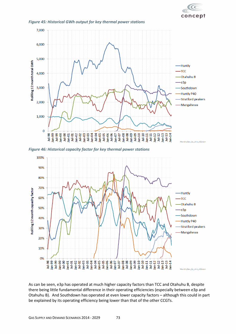
GAS SUPPLY AND DEMAND SCENARIOS 2014 - 2029 73
Figure 45: Historical GWh output for key thermal power stations
Figure 46: Historical capacity factor for key thermal power stations
As can be seen, e3p has operated at much higher capacity factors than TCC and Otahuhu B, despite there being little fundamental difference in their operating efficiencies (especially between e3p and Otahuhu B). And Southdown has operated at even lower capacity factors – although this could in part be explained by its operating efficiency being lower than that of the other CCGTs.

GAS SUPPLY AND DEMAND SCENARIOS 2014 - 2029 74
Going forward the relative contractual positions of the three main thermal generators is likely to change.
Genesis’ Kupe contract will continue to beyond 2020, likely resulting in it continuing to operate e3p at relatively high capacity factors. However, as illustrated in Figure 47 below, Contact’s gas contract position is due to change fundamentally.
Figure 47: Contact's contracted gas quantities
Source: “Contact 2014 Interim Results Presentation”, 18 Feb 2014
In 2014 Contact will no longer have a take-or-pay contract with OMV, and from 2015 onwards it will no-longer have any take-or-pay contracts. This is significant because the extent of running of TCC and Otahuhu B is considered to have been strongly influenced by Contact’s take-or-pay contracts, and that without such contracts, it is likely that the operation of Contact’s CCGTs would have been considerably less. In this respect it is notable that at the start of this year Contact indicated63 that:
Its plant has been operating when prices have been below the short-run marginal cost of a CCGT for more than 50% of the time; and
It would be unlikely to run TCC for winter 2014 unless conditions were relatively dry.
Thus, from 2015 and beyond, the only CCGT whose operation is likely to be kept at high levels because of high take-or-pay conditions in its gas contract is Genesis’s e3p station.
The extent of future operation of the other CCGTs, the OCGTs, and the Huntly’s coal units to meet the remaining (after-e3p) residual demand for thermal generation will be driven by the relative economics and flexibility of such plant.
63 “Contact 2014 Interim Results Presentation”, 18 Feb 2014

GAS SUPPLY AND DEMAND SCENARIOS 2014 - 2029 75
As indicated in Figure 44 above, with low coal and CO2 prices, Huntly can compete against CCGTs facing higher $/GJ gas prices. Further, if Genesis’s renegotiated Solid Energy coal contract has a take-or-pay element to it, this will drive some Huntly operation.
Flexibility will also be an important factor in determining plant utilisation. There is an increasing need for within-day flexibility because of the growth in wind generation. New Zealand’s hydro plants provide a large proportion of the required within-day flexibility, however there is still a significant requirement for thermal plant to increase and decrease its output to meet changing demand (and wind) situations. In this respect, CCGTs are not well suited to such a mode of operation: they have relatively high minimum operating levels (approximately 57% of full capacity), and they incur significant costs associated with starting-up. As a result, in order to be generating during periods when prices are profitable, they have to also be generating in periods ‘in-between’ that are loss making. In contrast, the Huntly units are able to drop to lower minimum generation levels, and are understood to have lower start-up costs. The most flexible plant of all are gas-fired OCGTs which incur much lower costs associated with ramping output up and down.
Analysis developed for the first supply / demand study illustrated that this difference in flexibility between CCGTs and OCGTs would result in CCGTs operating at significantly higher capacity factors than OCGTs – in large part because of CCGTs needing to operate during unprofitable periods in order to be able to capture the profitable periods.
What is less clear is whether in this situation of significant system overcapacity, it is possible that OCGTs may run ahead of CCGTs to meet the demand for flexible generation. i.e. below a certain capacity factor level it may be more profitable to not run a CCGT at all, and instead run OCGTs. This outcome appears consistent with Contact’s announcement earlier this year that it may not have the TCC CCGT in operation over the winter months, but would continue to operate its Stratford peakers.
A second flexibility dimension is seasonal flexibility. In this respect the cost is primarily associated with the cost of providing flexible fuel. Here, coal is considered to have a relatively low cost of providing seasonal flexibility –which is essentially the working capital cost associated with having a coal stockpile. This contrasts with gas, whose seasonal flexibility can come from two main sources:
‘Swinging’ gas production from gas fields. This can be expensive as it either requires reducing production in summer – which may mean forgoing associated liquids production and revenues – or re-injecting gas which is less costly but still involves some cost.
Using the Ahuroa gas storage facility. This facility allows gas produced during the summer to be stored underground, for use later in the winter. This can be a lower cost option than swinging a gas field, but there are still material costs associated with operating the gas storage facility (working capital costs associated with the pad64 gas, and capital and operating costs) which are materially higher cost than a coal stockpile.
A third flexibility dimension is the need to balance year-on-year variations in hydrology. Again, the costs of this are due to the costs of providing flexible fuel. In this dimension it becomes even more expensive for gas to compete with a coal stockpile to provide such flexibility. It could be possible for some major gas users such as Methanex to reduce their consumption to help provide gas during a dry year. However, as indicated in section 3.2.1, with current world Methanol prices this is likely to be a relatively expensive source of fuel flexibility.
Possible retirement of thermal generators
As noted earlier, Genesis has permanently decommissioned one Huntly unit, and put another into storage to be available for recall to meet dry-year events. The retirement decision is understood to reflect an expectation that the unit would earn insufficient revenue to cover both its fixed O&M costs
64 ‘Pad’ gas is the gas which is required in the facility to provide sufficient pressure for operation. It is not the ‘working’ gas which is cycled on a seasonal basis.

GAS SUPPLY AND DEMAND SCENARIOS 2014 - 2029 76
and potential stay-in-business capex costs. Further retirements of Huntly units are not expected in the short to medium term because:
As set out earlier on page 75, the lowest cost means of providing hydro-firming flexibility is considered to be the Huntly station operating on coal. It could be costly to meet this hydro-firming requirement with less than two Huntly units.
Much of the stay-in-business capex associated with the Huntly station relates to station capex that will enable the continued operation of all units in the station, rather than unit-specific capex which will only enable the continued operation of a specific unit. Because of this, if at least one unit is required to meet hydro-firming duties, it significantly reduces the marginal cost of keeping additional units operational.
The situation for the non-Genesis CCGTs is less certain. It is understood that both Contact and Mighty River are undertaking fundamental reviews of the future for their CCGTs. The issue for Contact’s two CCGTs especially are that they are facing potential stay-in-business capex associated with major mid-life maintenance overhauls.
It is possible that the reduced demand for thermal generation may not make it economic to invest to extend the lives of the CCGTs – particularly if the stay-in-business capex is significant, and expectations of demand growth indicate that it could be many years before demand growth reaches levels where the CCGTs could operate at more profitable levels.
For Contact’s Otahuhu B plant, one potential future option could be to convert the plant to operate in OCGT mode by removing the heat-recovery steam generator (HRSG). The reduction in operating efficiency from such a mode of operation could be offset by the combination of avoided stay-in-business capex associated with the HRSG plus the ability to operate more flexibly and thus, as described on page 75 above, avoid operating during unprofitable periods.
It is understood that converting to OCGT mode may not as easily achieved for the TCC CCGT.
3.3.5 Summary gas for power generation projections
Taking all of the above into consideration it is likely that:
The residual demand for thermal electricity generation will continue to decline over the next three years, primarily due to:
The commissioning of the Te Mihi geothermal station and Mill Creek wind farm
The reduction of demand from the Tiwai smelter from 2017.
The winding-off of Contact’s gas take-or-pay contracts, coupled with relatively low coal and CO2 prices, could see much of the reduction in thermal output over the next two to three years being borne by Contact’s CCGTs, with the balance being borne by the Huntly coal station and (to perhaps a lesser extent) the OCGTs.
Beyond 2017 it is likely that electricity demand generally will start to pick-up again, although not at the rates seen during the early part of the last decade. The rates of demand growth will be determined by factors such as GDP growth, population growth, and the extent of further energy efficiency changes. The fortunes of the Tiwai aluminium smelter will have a particularly significant impact on New Zealand demand growth
It is likely that in the early years of this period, much of this increased electricity demand will be met by increased output from existing thermal plant (most of which will be operating at low capacity factors and thus have spare capacity to take up this demand increase), rather than building new renewable plant. The extent to which this demand growth will be met by thermal vs new renewable, and what type of thermal (Huntly coal, CCGT or OCGT) will depend on:
General coal, gas, and CO2 prices. Thus, if fossil fuel and/or CO2 prices are high, the point at which it becomes economic to build new renewables will occur earlier. Similarly, if coal and CO2

GAS SUPPLY AND DEMAND SCENARIOS 2014 - 2029 77
prices are low, a greater proportion of the demand for thermal generation will be met by Huntly on coal rather than gas.
The cost of providing flexible generation on a within-day, seasonal, and dry-year/wet-year basis. This will influence which type of thermal plant (CCGT, OCGT, Huntly coal) will meet the demand for thermal generation.
The cost of new renewable plant. This will be strongly influenced by the NZ$ exchange rate. A fall in the NZ$ will make new renewables more expensive, and likely push-out the time at which new renewables start to be built again rather than running existing thermals harder.
The ‘shape’ of demand growth – e.g. if the economics of aluminium improve such as to make it profitable to produce aluminium at Tiwai above the levels in the Meridian contract this will be a baseload shape, whereas general commercial and residential demand growth will have a ‘peakier’ day/night and seasonal shape. As set out in Appendix A, baseload shapes are better suited to new renewables than peaky shapes;
The extent to which some thermal plant may have been retired in the interim – and thus will be unavailable to meet this increase in demand.
These are complex, inter-connected issues which to address comprehensively would require analysis using a mix of New Zealand power system models and specific financial models of individual generators and sources of fuel flexibility (i.e. coal stockpiles, gas storage, gas field swing, and gas re-injection).
Such detailed modelling is beyond the scope of this current study. However, high-level analysis been undertaken to help illustrate the nature and scale of these issues, and which has been used as a basis for developing reasonable scenario-based projections for future gas consumption from the power generation sector.
Appendix B describes the ‘model’ used to develop the power generation projections in the Gas_Dem model which has been released alongside this report.
Results
The following figures set out the projections for one particular combination of scenario parameters – namely the mid-point values for all such parameters, coupled with an assumption that Otahuhu B converts to OCGT mode in 2017, and the assumption that hydro inflows revert to the long-term mean based on the past 75 years’ worth of data.

GAS SUPPLY AND DEMAND SCENARIOS 2014 - 2029 78
Figure 48: Projected mean year power generation from different types of generation - area graph
Figure 49: Projected mean year power generation from different types of generation - line graph

GAS SUPPLY AND DEMAND SCENARIOS 2014 - 2029 79
Figure 50: Projected generation from different types of thermal plant
Figure 51: Projected gas consumption for power generation
These results indicate a likely continued reduction of gas demand for the power generation sector, at least until 2017. Beyond this time it is likely that gas demand for power generation will pick up again as existing thermal generators meet a growth in demand by increasing their capacity factors which will be

GAS SUPPLY AND DEMAND SCENARIOS 2014 - 2029 80
quite low by 2017 (TCC and Southdown are projected to have a mean hydrology year capacity factor of 20% in this scenario). Beyond a certain point, growth in demand reaches a level where it would be economic to build new renewables, rather than increase the capacity factor of existing thermal stations even further.
However, as Appendix B sets out, there are many different moving parts dictating the demand for thermal power generation and which thermal generators (Huntly, CCGTs, OCGTs) will meet such demand.
This is illustrated in Figure 52 below which shows the projections of mean year gas demand, including the extremes of such projections due to the combinations of electricity demand, CO2 and gas price assumptions.
Figure 52: Range of projections of gas demand for power generation in a mean hydrological year using 75 years’ of hydro inflows65
As discussed on page 66 previously, another key uncertainty relates to whether the relatively dry hydro inflows observed over the past 15 years will continue for the next decade or so, or whether inflows will revert to the mean levels measured over a 75 year period. The modelling shown above assumes that inflows are at the mean levels seen over the past 75 year period.
Figure 53 below shows the mean-year gas demand for power generation if mean hydro inflows are equivalent to the mean levels observed over the past 15 years.
65 Note: There is a slight difference between the central gas demand projection shown in Figure 51 and Figure 52. This is because they are showing results from different parts of the Gas_Dem model – one of which is based on MBIE data, and one based on Vector pipeline data – and there are differences in how some cogen plant in particular have been classified. These differences are not considered material to the analysis.

GAS SUPPLY AND DEMAND SCENARIOS 2014 - 2029 81
Figure 53: Range of projections of gas demand for power generation in a mean hydrological year using the most recent 15 years’ of hydro inflows
This results in approximately 15 PJ per year greater gas demand in a ‘mean’ hydro year (using this new, 15-year mean) than if the mean inflows were to revert to long-term averages based on 75 years’ of inflows.
This increase in power generation demand for gas due to using recent hydro inflows is a phenomenon which lasts for 5 to 8 years. Beyond that time, gas demand in the model is the same in both projections (i.e. using 75 years’ of inflows verus using 15 years’ of inflows) as it is assumed that new-build and retirement decisions will bring the system to the same supply / demand balance in both situations based on the relative economics of thermal generation versus new renewables.
To the extent that the past 15 years’ ‘dry’ conditions do continue for a further 5 to 15 years because of the Interdecadal Pacific Oscillation phenomenon discussed on page 66 previously, that is clearly favourable for gas producers. However, the flip side of this conclusion is that, if and when the weather flips out of this ‘dry’ IPO phase, it is likely that inflows will not revert to the 75 year mean levels used for this analysis, but will actually enter a wetter-than-average phase for 20 to 30 years. If and when this occurs, it is likely that significantly less thermal generation (and associated gas burn) will be required than indicated in the projections shown in Figure 52.
Discussion of results
Firstly, it should be appreciated that these results are from a highly simplified model which has only attempted to capture some of the inter-relationships between different drivers in a high-level fashion. Nonetheless, they indicate that there is a broad range of feasible outcomes for future power generation. Some of the key take-aways from this analysis are:
Gas demand from the power generation sector could drop significantly from historical levels to around 40 PJ per annum in a mean hydrological year. Key uncertainties are:
Tiwai demand. If Tiwai were to exit the market completely gas demand for power generation could fall significantly below this 40PJ level.

GAS SUPPLY AND DEMAND SCENARIOS 2014 - 2029 82
General non-Tiwai demand growth. If electricity demand growth were strong, the demand for gas for power generation could rise again to levels seen historically – although not for many years.
Hydrology. The last 15 years have been unusually dry compared with inflows measured over a 75 year time scale. If mean inflows follow the pattern seen over the past 15 years, the mean demand for thermal generation is likely to be some 1,800 GWh greater which, if it were largely met by gas-fired generation, could result in gas consumed for power generation being approximately 15 PJ greater than the above analysis indicates.
There is a core of thermal generation required to provide flexibility services – both to provide diurnal & seasonal demand variation, and to provide hydro-firming. Even in high CO2 and gas market scenarios it will be costly to displace this generation with renewables.
The 3 CCGTs other than e3p, and Huntly are likely to experience low capacity factors for at least the next three or four years. Unless Tiwai demand in particular increases, it is unlikely that all four plants would continue in their existing mode of operation. As discussed earlier, the relatively low cost of dry-year firming provided by Huntly coal suggests that one of the CCGTs may be more likely to exit or be re-configured to OCGT mode.
To the extent that one of the CCGTs does exit, its generation space (which will be predominantly providing flexible seasonal and diurnal generation at that point) will most likely be filled up in the short to medium-term by an existing thermal unit, rather than new renewables. However, in the long-term, such an exit or re-configuration of a CCGT is likely to result in new renewables being built earlier than would otherwise have been the case. This is because, in addition to providing flexible generation, it is likely that such an existing CCGT would also have started to meet growth in baseload demand. Without the plant, such a growth in baseload demand will need to be met by building new baseload capacity.
Overall, in descending order of influence, the key drivers of future gas demand for power generation are considered to be:
Future electricity demand growth
Future CO2 prices
Future gas prices
The retirement or re-configuration of existing thermal plant
The future cost of new, grid-scale renewables (which will in large part be driven by the future NZ$ exchange rate).
Such factors are inherently hard to predict. However, the power generation ‘model’ within the Gas_Dem model does enable users to examine the potential nature and scale of impacts from variations in these factors.
Lastly, it should also be appreciated that the values shown in the model are on a mean year basis. In the event of a dry year there could be some 2,500 GWh extra generation required. Similarly, in a wet year, some 2,500 GWh less generation may be required.
It is likely that a significant proportion of this swing will be met by Huntly on coal, although the precise extent will depend on relative coal, gas and CO2 prices at the time (and whether the Huntly unit has been retired or not). Nonetheless, year-on-year hydrology variations are likely to continue to result in significant year-on-year variations in the demand for gas. Functionality hasn’t been included within the Gas_Dem model to simulate the extent of such swing.
Comparison with 2012 study
The 2012 study had a fairly simplistic approach to projecting possible electricity generation gas demand, whereas this updated 2014 study has developed a substantially new modelling framework.

GAS SUPPLY AND DEMAND SCENARIOS 2014 - 2029 83
Figure 54 and Figure 55 below compare the projections between the two studies. Figure 54 shows the 2014 projections using 75 years’ worth of hydro inflows, whereas Figure 55 using 15 years’ worth of hydro inflows.
Figure 54: Comparison of projections of gas for power generation demand between the 2012 and the 2014 study (using 75 yrs hydro inflows)
Figure 55: Comparison of projections of gas for power generation demand between the 2012 and the 2014 study (using 15 yrs hydro inflows)

GAS SUPPLY AND DEMAND SCENARIOS 2014 - 2029 84
The main differences between the 2012 and 2014 projections of gas-fired generation are:
The 2014 study explicitly models the implications of hydrology, particularly the potential impact of inflows reverting to historical mean levels, as opposed to the relatively dry last 15 years.
The 2014 study explicitly models some of the dynamic interactions between demand and the different types of required generation (baseload, mid-merit, and peaking). This results in the upper limits of gas-fired generation in the sustained plentiful scenario being less than projected in the 2012 study, but conversely projects a higher level of gas-fired demand in the sustained tight scenario.

GAS SUPPLY AND DEMAND SCENARIOS 2014 - 2029 85
3.4 Industrial, commercial and residential demand
The last of the three gas demand segments is the direct use of gas by industrial, commercial and residential consumers. This direct use is primarily for energy purposes – i.e. space or water heating, or to generate process heat for industrial applications – not as a feedstock for a chemical process, or a fuel for electricity generation.
This category includes over 250,000 users, covering industrial (for example meat processors), commercial (for example hotels and restaurants), and residential customers.
3.4.1 Historical movements in demand
A number of different data sources have been used to analyse historical movements in gas demands for the direct use sectors.
The first is the MBIE quarterly energy data which is presented again in Figure 56 and Figure 57 below.
Figure 56: Historical sectoral gas demand - area graph
Source: Concept analysis using MBIE data

GAS SUPPLY AND DEMAND SCENARIOS 2014 - 2029 86
Figure 57: Historical sectoral gas demand - line graph
Source: Concept analysis using MBIE data
The key take-aways from the above figures are that:
Direct use of gas for energy represents the smallest segment of demand, accounting for approximately 21% of total New Zealand consumption in 2013. Within this segment, residential demand accounted for only 3.3% of total New Zealand consumption in 2013.
Direct use of gas for energy exhibits much less year-to-year variation in demand compared with the other users. Thus, while the petrochemical sector has exhibited extreme price sensitivity in terms of significantly altering consumption in response to the low-high-low wholesale prices seen over the last fifteen years, there has been no similar price sensitivity discernible for the direct use of gas for energy for the industrial, commercial and residential demand sectors.
The second source of data is MBIE data released as part of its “Energy in New Zealand” publication – a replacement to the previous “Energy Data File” publication. This data provides greater disaggregation on types of user within the broad “industrial” and “commercial” categories.
Figure 58 below show the historical movement of gas demand for the main industrial sectors, plus residential and commercial.

GAS SUPPLY AND DEMAND SCENARIOS 2014 - 2029 87
Figure 58: Historical gas demand for industrial sectors66
Source: Concept analysis using MBIE data
This data relies on submissions to Statistics New Zealand by retailers who are supplying gas to consumers. This is understood to have given rise to consistency issues as consumers switch between retailers who, for statistical submissions purposes, have classified such consumers differently. For example, the apparent spike in gas consumption for Dairy processing in 2011 appears suspicious, particularly as it occurs at the same time as an apparent drop in commercial consumption.
Nonetheless it is considered to be a reasonable indicator of general trends.
It is also broadly consistent with the last source of data which has been analysed to consider movement in demand for direct use of gas consumers – namely the daily quantities consumed at each of the Vector and Maui pipeline gates. This data is presented in Figure 59 below, and which is available in the publicly released model accompanying this supply / demand study.
66 It should be noted there are some classification differences between this data and the data shown in Figure 56 and Figure 57. In particular: - Agriculture & forestry is classed as ‘commercial’ in Figure 56 and Figure 57, yet is split out as a separate
category in Figure 58. - Major cogeneration plants are included in the ‘power generation’ category in Figure 56 and Figure 57, yet
appears to be included in the Steel (for the Glenbrook cogeneration plant) and Dairy (for the Te Rapa cogeneration plant in particular) categories in Figure 58.

GAS SUPPLY AND DEMAND SCENARIOS 2014 - 2029 88
Figure 59: Annual New Zealand gas demand measured at the Vector and Maui transmission gas gates (TJ)
Source: Concept analysis using various Oatis and GIC data
The data presented in Figure 59 is based on a couple of data sources:
Daily metered consumption at each transmission gas gate. Where a gas gate is dedicated to a particular consumer (e.g. a dairy factory, or meat works, or steel mill), that gate has been classified as belonging to that particular demand segment;
Daily allocation data from the Allocation Agent. This has been used for each gas gate which isn’t dedicated to a particular consumer, to split the consumption between time-of-use (‘ToU’) and non-time-of-use (‘Non’) consumer categories.
There are some classification differences between the data presented in the Figure 58 MBIE data and the Figure 59 gas gate data:
Some of the demand which has been classed as ‘ToU’ in the gas gate data will be identified as specific segments in the MBIE data. For example, a dairy factory which is connected to a distribution network (rather than directly connected to a dedicated transmission gas gate) will be included in the ‘ToU’ category for the gas gate data, but in the ‘Dairy’ category for the MBIE data.
The ‘Non’ segment in the gas gate data will likely include all residential consumption, plus some consumption which has been categorised as ‘commercial’ in the MBIE data.
However, in aggregate the trends between the two data sources appear fairly similar.
3.4.2 Projections of gas demand from the industrial, commercial and residential sectors
For the first gas supply / demand study in 2012, analysis was undertaken to determine whether relationships could be observed between sectoral demand and factors such as sectoral GDP and population. To the extent that such factors exist, they could then be used as a basis for developing projections of future demand, using projections of sectoral GDP and population as key inputs.
However, this 2012 analysis (which has been reproduced in Appendix C) identified that it is not feasible to robustly develop a projection approach based on projections of GDP and population – principally because gas is readily substitutable with other fuels for most energy applications.

GAS SUPPLY AND DEMAND SCENARIOS 2014 - 2029 89
Instead, a high-level approach has been developed which is based on observed historical growth rates, factored by consideration of the relative economics of gas versus other fuels for energy end use applications. This analysis of the relative economics of gas versus other fuels was studied in detail in the recent “Consumer Energy Options” study undertaken for Gas Industry Co.67
The key take-aways from the Consumer Energy Options analysis are:
The majority of gas for industrial use is for the generation of process heat, the majority of which is through the use of boilers to raise steam or hot water.
The majority of gas for residential or commercial use is for space or water heating
Gas is principally competing against
coal, biomass, and diesel for the provision of process heat
electricity for the provision of water heating
electricity and biomass (log-burners) for the provision of space heating
Gas is a strong winner for the provision of process heat based on its relatively low $/GJ fuel cost, and because the capital cost of solid-fuel boilers (for coal or biomass) is significant. Additionally, for food processing applications, it has other benefits in relation to the cleanliness of its combustion compared to solid fuel options which release particulates. For the wood sector, however, the presence of ‘free’ on-site biomass fuel often means that biomass options are more cost-effective than gas.
Gas is generally more cost effective than electricity for the provision of hot water. It also delivers additional benefits compared to cylinder-based options of not running out of water at times of peak use, and not taking up internal storage space.
Heat pumps are becoming more cost-effective than gas for space heating, but in some situations (particularly where consumers already have a gas connection for water heating purposes and a large heating load), gas heating can be cost competitive.
For most situations (i.e. for process heat, space, and water heating), it is generally not cost-effective to switch away from a fuel which has a higher variable cost to another which has a lower variable cost if the existing appliance does not need replacing. This is because the capital cost of the new appliance is often a significant component of the overall cost of providing useful energy, and for an existing appliance this is a sunk cost.
In general, therefore, the rate of change of gas demand for the industrial, commercial and residential sectors is likely to be relatively modest, driven by the gradual change in the demand for energy – which will principally be driven by GDP and population growth – overlaid with fuel switching dynamics as the relative economics of the different fuel options change with possible changes in fuel and CO2 prices.
This fuel switching dynamic is not likely to result in rapid rates of change because it is generally only cost-effective to switch away from a fuel if the existing energy appliance needs replacing. Given that domestic space and water heating appliances have useful lives of approximately 15 to 25 years, respectively, and industrial boilers can have useful lives of 30 to 40 years, fuel switching rates driven by the capital replacement cycle are likely to be relatively low.
Another source of data for considering possible future demand growth from the industrial, commercial and residential sector was stakeholder feedback from the interviews that were conducted as part of this study with key representatives from industrial sectors and pipeline operators.
67 The report can be found at this link: http://gasindustry.co.nz/sites/default/files/u12/consumer_energy_options_report_final_22_november_183275.1_0.pdf

GAS SUPPLY AND DEMAND SCENARIOS 2014 - 2029 90
With respect to the demand for gas as a process heat, in general, the feedback was consistent with the analysis set out in the Consumer Energy Options report. Stakeholders were not expecting significant changes in any of the industrial sectors, although they did expect some sectors to exhibit greater growth than others, particularly:
Dairy processing, with a number of new dairy processing factories possible over the next few years;
Horticulture, where a steady expansion in the number of hothouses is giving rise to a need for increased gas for heating; and
Refining, where a new fuel processing capability will come on line in 2016 meaning that less hydrocarbons from the refinery process will be diverted to produce process heat, meaning that more natural gas will be required.
With respect to the demand for gas for residential and commercial consumers, the pipeline operators were indicating that gas may be losing some ground to electricity for space heating, but that for water heating it was still competitive and represented a significant opportunity for growth in reticulated gas demand. In this respect, it was notable that the pipeline operators were indicating continued material growth in connections associated with new sub-divisions, and initiatives to bring gas to suburbs which have not had significant gas frontage to date.
Based on all the above, the demand estimates which have been used in the model to project the likely demand for gas in the gas supply scenarios are set out in Table 3 below
Table 3: Projected scenario growth rates for residential, commercial and industrial demand
These growth rates have been used to project demand for each of the pipeline regions even though, as set out on page 91 below, there are likely to be significant variances between different regions and at different times.

GAS SUPPLY AND DEMAND SCENARIOS 2014 - 2029 91
The growth rates set out above translate into the following projections of overall New Zealand gas demand from the industrial, commercial and residential sectors:
Figure 60: Projections of industrial, commercial and residential demand for direct use of gas for energy
Under the Plentiful Supply scenario, the rate of gas demand growth increases to approximately 1.8% per year, reflecting the combined effect of economic growth and some expansion in gas market share relative to other primary energy sources.
Under the Moderate Supply scenario, gas demand is projected to grow at around 0.6% per year. Under the Tight Supply scenario, gas demand is projected to modestly decline from current levels at approximately -0.75% per year, but remain around 35 PJ/year. This reflects the relatively limited scope for further cost-effective fuel substitution away from gas among large industrial users, and the fact that underlying well-head gas costs are a modest proportion of delivered gas prices for residential and commercial users.
It should be noted that the above projections are considered indicative of the types of long-run average rates of growth that could be experienced for each of the scenarios. This compares with year-to-year rates of growth which can experience significantly greater variation due to factors such as major point sources of load coming on or off the system at single points of time. This variation becomes even more pronounced as smaller and smaller geographic sections of the system are considered. This is illustrated in Figure 61 below which shows that the rates of growth for particular consumer segments are less extreme when considered on a whole of North Island basis than for the individual pipeline systems.

GAS SUPPLY AND DEMAND SCENARIOS 2014 - 2029 92
Figure 61: Historical growth rates for demand segments for different regions and time periods
3.4.3 Comparison with 2012 study
Table 4 below compares the scenario growth rates assumed for the different direct use load segments, for the 2012 and 2014 studies.
Table 4: Comparison between 2012 and 2014 study direct use for energy scenario growth rates
The key changes between the 2012 and 2014 studies are:
For space and water heating demand, the 2014 study has reduced rates of growth due to assumptions around the extent of uptake of heat pumps.
For major industrial demand the 2014 study has increased growth rates for the dairy, paper and steel sectors, and reduced rates of growth for the meat sector. These revised assumptions were based on discussions with various industry stakeholders.

GAS SUPPLY AND DEMAND SCENARIOS 2014 - 2029 93
3.5 Summary projections of gas demand
Figure 62 below combines the various petrochemical, power generation, and direct use for energy gas demand scenarios set out in the previous sections. In addition to the range of gas demand futures arising from future gas market scenarios, it also shows the extremes caused by the variation in demand for power generation arising from other drivers such as electricity demand growth and future CO2 prices.
Figure 62: Projections of total New Zealand gas demand under different scenarios (assuming mean hydrology based on 75 years’ of past inflows)
As can be seen, there is a significant range of possible gas demands looking 15 years into the future.
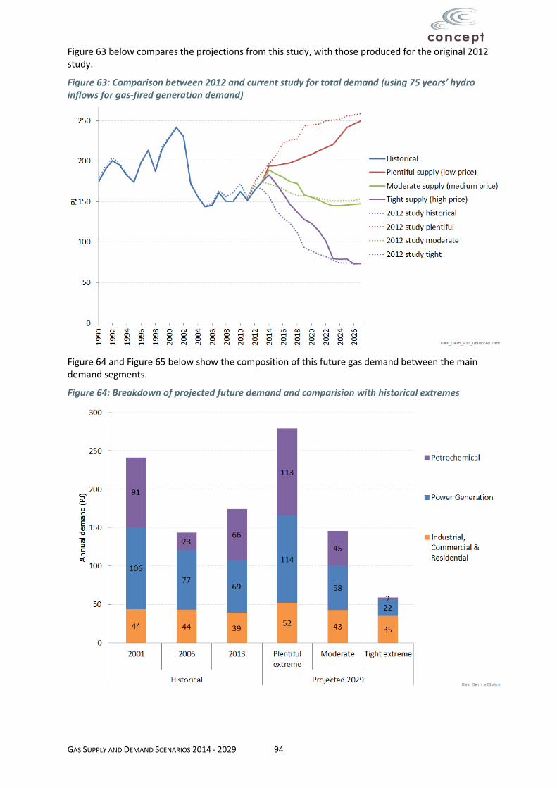
GAS SUPPLY AND DEMAND SCENARIOS 2014 - 2029 94
Figure 63 below compares the projections from this study, with those produced for the original 2012 study.
Figure 63: Comparison between 2012 and current study for total demand (using 75 years’ hydro inflows for gas-fired generation demand)
Figure 64 and Figure 65 below show the composition of this future gas demand between the main demand segments.
Figure 64: Breakdown of projected future demand and comparision with historical extremes

GAS SUPPLY AND DEMAND SCENARIOS 2014 - 2029 95
Figure 65: Breakdown of projected future demand and comparison with historical extremes - by sector
As can be seen, the key sectors that are likely to exhibit significant variations in demand are the power generation and petrochemical sectors.
One implication of this is that pipeline systems with power generation demand are going to exhibit far greater future demand uncertainty than those without power generation. (Noting that petrochemical demand is located close to gas wellheads, and thus is not going to be a major determinant of pipeline demand).
To illustrate this, Figure 66 and Figure 67 show projections for two very different pipeline systems:
Maui pipeline demand North of the Mokau compressor (which has the Huntly, e3p, Otahuhu B and Southdown power stations); and
The Vector South transmission system, which has no significant thermal power generation attached to it.

GAS SUPPLY AND DEMAND SCENARIOS 2014 - 2029 96
Figure 66: Projections of annual demand North of the Mokau compressor (for mean hydrology power generation using 75 years’ of inflows)
It should be noted that this demand is for mean-hydrology year power generation. In the event of a dry or wet year, demand for power generation could be considerably greater or less than these levels.
Figure 67: Projections of annual demand for the Vector South transmission system

GAS SUPPLY AND DEMAND SCENARIOS 2014 - 2029 97
Hydrology uncertainty
As previously discussed on page 81, one other key uncertainty relates to whether the relatively dry conditions experienced over the last 15 years will continue for a further 5 to 15 years, or whether hydro inflows will revert to mean levels (as has been assumed for the above analysis) – or even revert to a wetter-than-average phase which lasts for 20 to 30 years.
To illustrate the scale of this impact, Figure 68 and Figure 69 below present the same data as in Figure 62 and Figure 66, respectively, but assuming mean hydro inflows are equivalent to the mean experienced over the past 15 years, rather than the past 75 years.
Figure 68: Projections of total New Zealand gas demand under different scenarios (assuming mean hydrology based on the past 15 years’ of inflows)

GAS SUPPLY AND DEMAND SCENARIOS 2014 - 2029 98
Figure 69: Projections of annual demand North of the Mokau compressor (for mean hydrology power generation using the past 15 years’ of inflows)
As can be seen, the demand for gas for power generation is significantly greater if mean hydro inflows continue based on the pattern observed over the past 15 years, rather than reverting to the 75 years mean.

GAS SUPPLY AND DEMAND SCENARIOS 2014 - 2029 99
4 Gas demand scenarios – peak demand
Chapter summary
When considering the implications of future demand on pipeline investments it is necessary to project peak demands, not annual demands. For some pipelines peak-day demand is critical, whereas for others it is the peak-week demand – with the difference being due to how much line pack each pipeline has available.
Different demand segments make different contributions to system peak demands due to different seasonal consumption patterns, and different weather sensitivities (i.e. demand being linked to outside temperature). The two segments which have the greatest weather-sensitivity and seasonal consumption patterns are the Non-ToU (i.e. mass-market) segment, and power generation.
The apparent drop in peak demand from 2011 for many pipeline regions is largely due to weather in subsequent years not being as severe as during the August 2011 extreme weather event. On a weather-corrected basis, the peak demands across the years are much more similar.
One option for addressing peak demand is to temporarily interrupt some demand segments. Historically, the Marsden Point refinery is the only material load which has been on an interruptible contract. However, a significant un-tapped potential exists from the power generation sector and some industrial process heat demands that would be much cheaper than investing in upgrading pipeline capacity.
The two pipeline systems which have received greatest focus on the potential future need to upgrade pipeline capacity are the Vector North system, and the Mokau compressor serving all Maui pipeline load north of this point. Study projections indicate that it is extremely unlikely such capacity upgrades will be required, particularly due to:
The potential for interruption from power generation and some industrial process heat loads;
The possibility that the Otahuhu B CCGT power station could be re-configured to OCGT mode.
4.1 Analysis of peak demand drivers
The demand scenarios set out in section 3 were described primarily in terms of annual quantities. This section uses this annual information to develop projections of peak demand in each year. This subsequent step is necessary because the critical factor determining the need for pipeline investment is gas demand at times of peak usage, rather than annual demand.
This is because gas pipes have a finite amount of capacity to transport gas. While the levels of gas being transported remain below this capacity, the costs of operation are relatively low – largely comprising the operating costs associated with compressors and the like to flow the gas along the network.

GAS SUPPLY AND DEMAND SCENARIOS 2014 - 2029 100
However, if demand rises above this capacity level, gas could not be transported without breaching safety thresholds. Once this level of demand is reached, some gas demand will need to be curtailed to keep pipeline flows below this capacity limit. Greater flows of gas cannot be realised until investment is made in the pipeline to upgrade its capacity.
At the time the 2012 study was undertaken, the Vector North transmission system was the principal Vector transmission system where concerns were being raised that such capacity constraints were being reached. Concerns too had been raised that the capacity of the Maui pipeline north of the Mokau compressor may reach its limits at some point in the future, thereby necessitating an upgrade to the compressor.
Since the 2012 study, some of the concern relating to the these systems has eased – in large part because of the decline in the demand for thermal generation which allowed for some contracted firm capacity to be converted into interruptible. It is understood that all requests for capacity in the North pipeline have been met for the present year.
Nonetheless, pipeline capacity allocation is still an issue under active consideration – particularly for the Vector North system.
Accordingly, this part of the study has been updated for this 2014 report, and uses the Vector North system as an example. However, the model and associated analysis is capable of looking at all systems using the same broad framework.
Virtually all of the graphs shown in this section of the report are from the Gas_Dem model that has been released in association with this study. Accordingly, parties can use the model to look at other geographical systems if they wish.
As shown in Figure 70 below, there is a wide variation in the level of daily gas demand on the Vector North system. Patterns that can be seen include a weekly cycle, a seasonal (winter-summer) variation, public holiday effects, plus there can be significant year-to-year and week-to-week variation.
Figure 70: Historical total daily gas demand on Vector North system

GAS SUPPLY AND DEMAND SCENARIOS 2014 - 2029 101
Figure 71 re-arranges the data from Figure 70 into a duration curve format. This more clearly illustrates how for the vast majority of the time, gas demand is significantly below peak levels.
Figure 71: Duration curves of historical total daily gas demand on Vector North system
The duration curves also indicate that between 2004 and 2011, demand on the North system was generally getting steadily peakier, as indicated by the reducing load factor shown in the graph key.68 However, recently the load factor has improved, as is illustrated further in Figure 72 below.
68 The load factor is calculated as the average demand level divided by the peak demand level.

GAS SUPPLY AND DEMAND SCENARIOS 2014 - 2029 102
Figure 72: Relative movements in annual and peak demand for the North system
Figure 73 sets out further analysis to understand what has been contributing to the peak, and the year-to-year changes in its magnitude.
Figure 73: Historical sectoral composition of peak day demand for Vector North system (GJ)

GAS SUPPLY AND DEMAND SCENARIOS 2014 - 2029 103
Power generation has been the most significant contributor to peak day demand on the North system. Also, as illustrated in Figure 72 above, it can be seen that there has been less year-on-year change in peak demand than annual demand.
Although it is often useful to consider things in peak day terms (for example “maximum daily quantity”, or MDQ, is a key parameter in most gas contracts), the critical time period for pipeline capacity issues for the North system is understood to be closer to a week. This is because of the ability of line pack to absorb a one-off peak day, but after a series of consecutive very high daily demands, line pack levels will eventually drop below the critical threshold.
Accordingly, Figure 74 show analysis to help understand what contributes to peak week demand on the Vector North system. (Week is considered to be the working week of Monday to Friday, rather than the calendar week of Monday to Sunday).
Figure 74: Historical sectoral composition of peak week demand for Vector North system (GJ)
As can be seen, the proportions of different sectors are broadly similar to peak day demand.
Figure 75 further illustrates how the proportions of the different sectors to the North system demand total vary according to whether demand is measured as an annual quantity, or on some measure of peak.

GAS SUPPLY AND DEMAND SCENARIOS 2014 - 2029 104
Figure 75: Sectoral proportions of gas use for 2013 for different time periods for Vector North system
Due to the inherent variability of demand driven by factors such as the weather, and ‘natural’ randomness in the coincident level of demand from consumers, to model peak demand necessarily requires the ability to consider the probabilities of demand reaching certain levels, and thus estimating what a (say) 1-in-20 year or 1-in-50 year level of peak demand would be. This exercise has some key inherent challenges:
There is only a limited historical gas demand data set (just over ten years), meaning that just considering this data alone would make it hard to infer what a 1-in-50 year peak demand, say, might look like;
There is a need to be able to consider peak demand over different lengths of time, ranging from a day through to a week, given that the critical time-period for different pipelines can vary;
Different demand sectors exhibit different seasonal and diurnal patterns, and different temperature sensitivities, yet the proportions of these different sectors has varied during the historical data series, and is likely to vary further into the future.
To address these issues, a statistical model was developed for the 2012 study which sought to estimate the relationship between demand and key observable drivers (namely temperature and temporal parameters (for example day of week, month of year, public holidays)). This model is described in detail in Appendix D.
It broad terms, it enabled projections of peak demand for the different pipeline systems to be developed based on the underlying assumptions regarding annual demand growth for the different sectors as described in section 3, assuming that historical peak/annual relationships are maintained for each sub-segment of gas usage (power generation, industrial etc).
The statistical analysis revealed that, due to factors such as the extreme temperature-dependency of sectors such as Non-ToU demand, the overall system load duration curve is quite ‘peaky’. As Figure 76 below illustrates, 8.4 % of the pipeline capacity used by non-generation demand is required for only 0.5 % of the time.

GAS SUPPLY AND DEMAND SCENARIOS 2014 - 2029 105
Figure 76: Modelled duration curves of non-generation demand on the North System
The analysis further revealed that there is a significant range of possible peak day and peak week demands that may be experienced in a year due to the year-on-year variability introduced by the weather and the ‘natural’ randomness of demand. For example, Figure 77 below illustrates the modelled range of possible non-generation peak outcomes in the North system.
Figure 77: Modelled range of possible non-generation peak outcomes in the Vector North system
Thus, this modelling suggests that the range between maximum and minimum peak possible peak week outcomes is equivalent to 16.4% of mean peak week demand, and that a 1 in 10 year peak week

GAS SUPPLY AND DEMAND SCENARIOS 2014 - 2029 106
demand would be 4.9% higher than the mean peak week, but a 1 in 99 year peak week demand would be 8.1% higher.
It is understood that one reason 2011 was a relatively peaky year was because of the extreme weather event in August 2011. The analysis set out in Appendix D revealed this to be a 1-in-95 year event. This is further illustrated by the relative movement of annual versus peak demand for the ‘Non’-ToU segment (i.e. mass-market customers which are non-TOU metered) as shown in Figure 78.
Figure 78: Relative movements in annual and peak demand for North system for the 'Non'-ToU segment
Thus the improving load factor for the North System seen in 2012 and 2013 (as can be seen from Figure 71 and Figure 72 shown previously) may in fact be a reflection that these years did not experience as severe a weather event as occurred in 2011.
On a weather-corrected basis, therefore it is possible that there has been little change in the peakiness of demand on the North system.
This raises issues as to the appropriate security standard Vector should operate the pipeline with respect to allocating capacity such that peak demand is not expected to exceed a 1 in ‘x’ year event. However, it is not within the scope of this study to consider what such a security standard should be.
Further, such statistical analysis makes no consideration of the potential for changes in consumer behaviour at times of peak demand. Such changes may emerge if consumers face altered price signals as a result of changes in the design of pipeline pricing and access arrangements – in particular if they move to an interruptible rather than firm contract for pipeline capacity.
Analysis on interruptibility was undertaken for the 2012 study, and is included again in this study as Appendix E – albeit with some aspects updated with recent data where appropriate.
This analysis reveals that there is a lot of potential for interruption if peak demands start to approach the limits for a pipeline – particularly from the power generation sector.

GAS SUPPLY AND DEMAND SCENARIOS 2014 - 2029 107
4.2 Projections of peak demand
The model that has been released with this report includes projections of peak week and peak day demand for all the different geographic systems (and groupings of systems).
These projections have been developed based on the underlying annual demand projections set out in section 3 for each customer use segment for the different gas market scenarios.
Rather than use the statistical model described in Appendix D to develop the projections a simpler approach was adopted as follows:
the historical ratios between peak week (or day) demand and annual demand for each customer use segment for each geographical system were calculated for each of the twelve historical years in the data set
the maximum ratio was chosen as being indicative of the relationship between annual demand and peak demand during a severe weather event. (In most cases, this results in the ratio from 2011 being chosen)
this maximum ratio is applied to the projection of annual demand to indicate a realistic severe weather peak week (or day) level of demand that is consistent with the assumptions about underlying demand growth.
There are two customer segments where this approach wasn’t applied:
Firstly, because the refinery has had an interruptible contract historically, its historical demand during years with severe peak weeks is likely to have been less than in years with milder peak weeks. Accordingly, the observed ratio between peak and annual for 2011 is used as the basis for projecting future refinery demand during severe peak weeks.
Secondly, peak week / day gas demand from power generators has been modelled explicitly based on the underlying scenarios for power generation set out in section 3.3.
The peak week gas demand for power generation has not been calculated based on some relationship between projected annual generation and peak week demand. Instead, potential peak demand from power generation assumes that the gas fired generator is operating at full capacity for the duration of the peak.69 Such an outcome could theoretically occur during an intense cold snap which happened to coincide with a relatively dry and calm (i.e. not windy) period. However, this is considered to be very unlikely – particularly for OCGT-type generators.
A second line is also shown which shows what the likely demand for gas for the power stations were to be during such a cold & dry peak period if they were operating at ‘full interruptibility’ as described in Appendix E. This takes account of the different abilities of gas-fired power generators to scale back generation during off-peak periods.70
Huntly’s gas demand during peak weeks is assumed to be zero for the ‘full interruptibility’ scenario (i.e. it is assumed to be operating completely on coal), but for the theoretical maximum level of peak gas
69 For the peak week, this is factored down by 95% - i.e. assuming that it is likely that there would be some turning down at some point during the week. For consideration of summation of multiple geographic systems, there is also a coincident factor which scales down the amount of demand across all the generators. Based on observation of historical data this coincident scaling factor has been set to 90% for peak days, and 93% for peak weeks. However, it should be appreciated that there is progressively greater uncertainty as to the total coincident peak system generation across all thermal generators when looking at progressively greater regions. 70 The large CCGTs are assumed to have a min-gen level of 57% - which translates to a reduced level of generation across the whole day (i.e. including the periods when they are at max gen at peak) of 68%, being the level of generation during peak at full interruptibility. The corresponding min-gen values for Southdown and OCGTs are 3% and 0% (i.e. they can easily turn off completely), which gives rise to peak interruptibility values of 28% and 25%, respectively

GAS SUPPLY AND DEMAND SCENARIOS 2014 - 2029 108
demand, the level of Huntly gas varies according to the underlying gas and CO2 market scenario – e.g. if CO2 prices are high, it is assumed to burn less coal than if CO2 prices are low.
The future status of Otahuhu B and TCC is also taken into account for the projection – i.e. whether Otahuhu B is converted to OCGT mode (in which case it will have much greater interruption capability), or whether TCC is retired.
However, what this approach does not do is take account of the extent to which there may be overcapacity in the New Zealand electricity market, such that even during a cold & dry peak period there will not be the need to operate all thermals at full capacity. This is illustrated by Table 5 which shows some graphs taken from the model for two very different scenarios:
A future with extremely low electricity demand (including the closure of Tiwai). The graphs for this future are shown on the first row of the table
A future with high electricity demand growth, and low gas and CO2 prices. The graphs for this future are shown on the second row of the table
For each scenario, the left-hand graph shows annual gas demand for the North system, whereas the right-hand graph shows projected peak week demand.

GAS SUPPLY AND DEMAND SCENARIOS 2014 - 2029 109
Table 5: Projected mean-hydrology annual, and peak week demand for the North system for very different power generation scenarios
Representative low thermal power generation demand scenario
Representative high thermal power generation demand scenario

GAS SUPPLY AND DEMAND SCENARIOS 2014 - 2029 110
In the first scenario in Table 5, annual gas demand on the North system plummets – driven by the huge decline in the need for gas-fired power generation from Otahuhu B and Southdown. In the second scenario, annual gas demand falls during the period 2014 to 2016, but then is projected to recover significantly due to the growth in demand for the generation from Otahuhu B and Southdown.
However, the projected potential peak week demand for both scenarios is the same. This is because the methodology described above is based on the physical potential peak week demand for such plant, rather than the likely peak week demand for such plant.
In order to project the likely peak week generation demand would require more sophisticated analysis that considered the whole electricity system and the likely extent to which the system was in a situation of relative over- or under-capacity in any given future year.
Such analysis is beyond the scope of this study.
However, based on the considerations set out in section 3.3 above, it is likely that New Zealand’s power generation sector will be in a state of over-capacity for the next few years, and that this will result in reduced peak demands from the power generation sector.
On balance, it would therefore appear likely that the North system will not face capacity constraints in the short to medium term.
The extent to which this situation will continue will depend on a number of different factors including:
The extent of electricity demand growth (or decline)
Whether existing thermal power stations are retired or re-configured – particularly the three main CCGTs and the remaining two Huntly units.
Future gas, coal and CO2 prices, and the price of new renewables
If the Otahuhu B power station were converted to OCGT mode, it is likely that the North system would not face capacity constraints requiring investment in new pipeline capacity for the foreseeable future.
In this respect, it is notable that the Vector gas transmission asset management plan71 is projecting a significant decline in the contractual capacity for the Otahuhu B and Southdown power stations by 2024.
Analysis of potential peak capacity issues for the Maui pipeline north of Mokau
This apparent disconnect between projections of annual demand and theoretical uninterrupted peak demand is even more stark when considering the Maui pipeline north of Mokau.
Table 6 below shows the same type of analysis for the Maui pipeline north of Mokau as was done for the Vector North system shown above in Table 5 on page 109. The only difference is that peak day demand is shown for Maui north of Mokau, whereas peak week demand is shown for the Vector North system. This is because of differences in the quantities of line pack in the two systems relative to the size of the pipelines and their key demands.
71 Vector 2014, Gas Transmission Asset Management Plan Update, Information Disclosure 2014, http://vector.co.nz/documents/101943/102848/Gas+Transmission+AMP+Update+2014+FINAL.pdf/dd4a97f9-3cce-4a42-bdc6-a3ffc5cd8992,
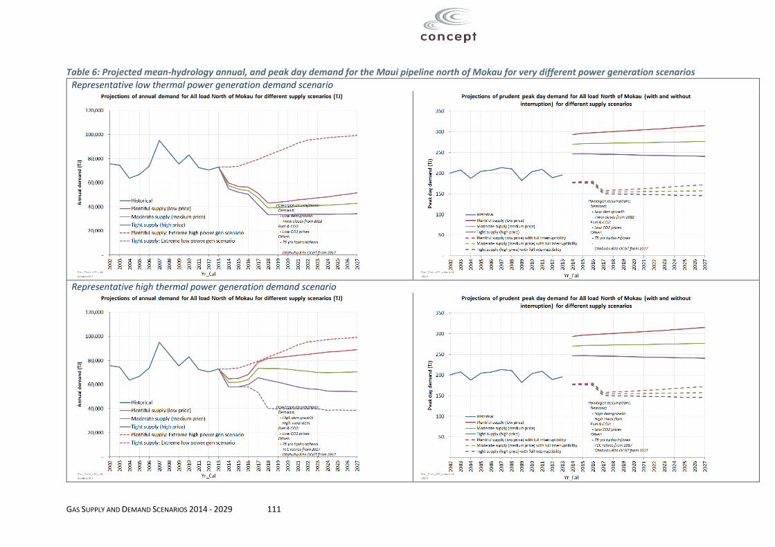
GAS SUPPLY AND DEMAND SCENARIOS 2014 - 2029 111
Table 6: Projected mean-hydrology annual, and peak day demand for the Maui pipeline north of Mokau for very different power generation scenarios
Representative low thermal power generation demand scenario
Representative high thermal power generation demand scenario

GAS SUPPLY AND DEMAND SCENARIOS 2014 - 2029 112
Whereas the Vector North system only has two material gas-fired power stations – the 400 MW Otahuhu B station, and the 175 MW Southdown station – the Maui pipeline north of Mokau additionally has three more power stations: the 2(3)72 x 250MW dual-fuelled Huntly thermal power station, the 400MW e3p CCGT, and the 45MW P40 OCGT – all of which are located at the Huntly site.
Having five thermal power stations being fed by the Maui pipeline north of Mokau means that there is greater likelihood of diversity among the power stations – i.e. the chances of all five stations operating at full capacity for a day are less than the chances of just one station operating at full capacity for a day.
This is further complicated by the dual-fuel nature of the Huntly power station. For the projections of annual demand and uninterrupted peak day demand, the proportions of coal : gas generation at the Huntly station vary according to the gas price scenario. Thus, in the low gas price scenario, the proportion of coal burnt in the station is relatively low, whereas in the high gas price scenario, the proportion of coal burnt in the station is relatively high.
However, as set out previously on page 107, in the ‘full interruptibility’ scenarios, Huntly is assumed to switch completely to burning coal, with gas demand consequently being low.
Thus, when taking into consideration:
- the potential for ‘economic’ interruptibility for gas-fired power stations (as set out in Appendix E);
- the likely diversity factor from multiple gas-fired power stations; and - the extent of over-supply in the electricity system in the short-to-medium term
it does not appear likely that peak day demand for the Maui pipeline north of the Mokau system will rise to levels which would require investment to increase the capacity of the pipeline. This is illustrated by the ‘full interruptibility’ lines for the peak day projections not rising above observed historical peak day demands over the full period of the projection.
72 The Huntly thermal power station originally had 4 x 250 MW units. Genesis has permanently retired one unit, and put a second unit into ‘dry year storage’ – i.e. mothballed, but with the ability to be recalled in the event of it being needed to provide cover for a severe dry year.

GAS SUPPLY AND DEMAND SCENARIOS 2014 - 2029 113
Appendix A. Analysis on the extent to which electricity demand growth will be met by thermal versus renewable generation
A number of stakeholders have suggested that the observed displacement of existing thermals by new-build renewables will likely continue over the next ten to fifteen years until such point as New Zealand’s electricity is entirely renewable.
Others have suggested that while renewables may displace thermals from baseload operation – but only in futures of high CO2 and gas prices – the economics of building plant to operate to meet the significant within-day and within-year variations in demand are such that it is extremely unlikely that thermal plant will be displaced from meeting these duties.
This section sets out analysis which considers these issues, and develops a framework which has been used to estimate the likely demand for thermal generation for different fuel and CO2 market scenarios.
The seasonal and diurnal variation in demand gives rise to a need for some generation to operate at low capacity factors
Demand varies significantly on a within-day (diurnal)73, and within-year (seasonal) basis. This is illustrated schematically in Figure 79 below, which also shows how this variation in demand gives rise to a need for some generators to only operate for part of the time.
Figure 79: Illustration of the variation in demand giving rise to a need for low capacity factor generation
Figure 79 also introduces the concept of different types of generator operation being categorised based on how frequently it operates. Thus:
Plant which operates all day, every day throughout the year is termed ‘baseload’.
At the other extreme, plant which operates only for relatively few periods of peak demand is termed ‘peaking’; and
Plant which operates somewhere between these levels is termed ‘mid-merit’.
73 The diurnal variation in demand also follows a weekday / weekend pattern, with weekend demand being materially less than weekday demand.

GAS SUPPLY AND DEMAND SCENARIOS 2014 - 2029 114
In reality there is no hard definition delineating these different modes of operation – e.g. when a plant operates so infrequently that it becomes classed as peaking rather than mid-merit – but the concept is a useful one for considering the economics of different modes of operation.
Figure 79 also introduces the concept of a duration curve being used to consider the different capacity factors of operation. The capacity factor of a power station is a measure of how often it operates. It simply equals the average MW output across the year, divided by the MW capacity of the station. A station which operated at full output for every hour of the year would have a capacity factor of 100%74, whereas a ‘peaker’ station may have a capacity factor less than 5% - i.e. it only operates for a relatively few days in the year.
The characteristics of geothermal and wind plant make them not cost-effective options for meeting low capacity factor operation
Figure 80 below shows the break-even cost of baseload generation from different types of existing and hypothetical new generation.75
Figure 80: Estimates of the break-even costs of baseload operation for different plant76
As discussed on page 71 of the main report, this graph reveals that for meeting growth in baseload demand:
The cheapest option is running existing thermals harder, but only if:
They have spare capacity; and
74 Because of maintenance outages, even so-called ‘baseload’ power stations will generally have capacity factors of around 90%-95%. 75 A hypothetical new geothermal plant has been included as being broadly representative of the cost of new renewables, including wind plant. This is because more geothermal options appear more cost effective than wind for meeting demand growth in New Zealand for the next 10 to 15 years. However, it should be appreciated that the cost of new renewables varies on a site-by-site basis, and some renewable options will be more expensive that the approximately $80/MWh value shown here – and some potentially less than this value. 76 VOM = Variable operating & maintenance costs. FOM = Fixed operating & maintenance costs.

GAS SUPPLY AND DEMAND SCENARIOS 2014 - 2029 115
Fuel and CO2 prices are relatively low. Huntly coal in particular is sensitive to high CO2 prices, whereas CCGTs are still more economic than building new renewables even for relatively high CO2 prices.
If there is no spare capacity from existing thermals, the next cheapest option is building new renewables rather than building a new CCGT, except if gas and CO2 prices were very low – and likely to remain so for the 10-15 years that an investor would seek to recover their capital costs. For CO2 prices in particular, this does not appear to be a realistic outlook.77
Some of the cost categories in Figure 80 are variable – i.e. they vary directly in proportion to the number of MWh generated. These are principally fuel costs, CO2 costs, and variable operations & maintenance (VOM) costs.
However, two of the cost categories are fixed:
Fixed O&M costs – being the annual costs incurred in keeping the plant operational. This typically covers items such as labour, rates, some transmission costs78, and some maintenance which does not vary with hours of operation.
Capital – being the costs incurred in building the plant in the first place.
Treatment of such costs is critical in understanding the relative economics of different plant operating in low capacity factor, mid-merit or peaking modes.
In order to translate these costs which don’t vary with the number of MWh generated into a $/MWh value it is necessary to divide the total $ cost incurred in a year by the number of MWh generated in a year.79
This variablisation of fixed costs enables comparison of the overall costs of different types of generator to determine which is likely to be most economic.
For comparison of the relative costs of baseload operation the number of MWh generated in a year is simply the MW capacity of the plant * 8,760 hours * (1- maintenance outage factor).
Typical maintenance outage factors range from 5 to 10%, giving rise to typical capacity factors for baseload plant being 90 to 95%, rather than 100%. These typical values have been used for comparison of the baseload operating costs of the different options set out in Figure 80 above.
For mid-merit and peaking modes of operation, capacity factors can be substantially less than 90%, meaning that any fixed O&M and capital costs will need to be recovered over much fewer MWh. As the denominator in this $/MWh calculation gets progressively smaller with progressively lower capacity factors, the $/MWh cost associated with such fixed and capital cost recovery gets progressively higher.
To illustrate the effect of this, Figure 81 and Figure 82 below show the costs for five different types of existing and new plant for a hypothetical set of fuel and CO2 prices.
For the fuel and CO2 prices used in Figure 81 below the most economic form of new baseload generation is the new geothermal plant. In this example the cost of the geothermal plant is also cheaper than the cost of operating the existing Huntly unit on coal, and therefore it would be economic to build such a geothermal plant to displace Huntly from baseload operation – if it were to be operating
77 There is a growing international consensus that climate change is significant, and the social costs are likely to be materially higher than reflected in the current low levels of CO2 prices. What is not clear is whether and how these costs will be reflected in a cost to GHG emitters over the next 10-15 years. 78 For example some transmission connection costs. 79 For the capital component of costs, the numerator is not the full capital cost, but the capital cost to be recovered each year. This annual capital recovery is based on the number of years over which the capital cost is to be recovered and the owner’s cost of capital – i.e. the financing cost associated with building a plant. For example, a hypothetical plant which cost $100m to build and whose costs were to be recovered over 10 years using a 10% cost of capital, would have an annual capital recovery charge of $16.25m, not $10m per year.

GAS SUPPLY AND DEMAND SCENARIOS 2014 - 2029 116
in such a fashion. However, it is not cheaper than the existing CCGT and it would therefore not be economic to be built to displace the existing CCGT from baseload operation.
Figure 81: Baseload costs for five different types of plant for a hypothetical fuel and CO2 market scenario
However, for lower capacity factor modes of operation, the FOM and Capital components of cost will need to be spread over progressively smaller MWh volumes. This is illustrated in Figure 82 below, which shows that plant which have a high proportion of fixed O&M and capital costs are uneconomic to operate at low capacity factors compared to plant with a low proportion of fixed O&M and capital costs.
The most cost-effective means of meeting such mid-merit and peaking duties is operating existing thermal stations harder – or building new peaking thermal stations such as OCGTs if the existing stations don’t have any spare capacity.
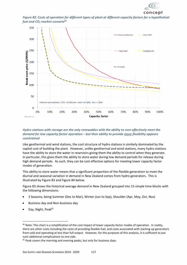
GAS SUPPLY AND DEMAND SCENARIOS 2014 - 2029 117
Figure 82: Costs of operation for different types of plant at different capacity factors for a hypothetical fuel and CO2 market scenario80
Hydro stations with storage are the only renewables with the ability to cost-effectively meet the demand for low capacity factor operation – but their ability to provide more flexibility appears constrained
Like geothermal and wind stations, the cost structure of hydro stations is similarly dominated by the capital cost of building the plant. However, unlike geothermal and wind stations, many hydro stations have the ability to store the water in reservoirs giving them the ability to control when they generate. In particular, this gives them the ability to store water during low demand periods for release during high demand periods. As such, they can be cost effective options for meeting lower capacity factor modes of generation.
This ability to store water means that a significant proportion of the flexible generation to meet the diurnal and seasonal variation in demand in New Zealand comes from hydro generators. This is illustrated by Figure 83 and Figure 84 below.
Figure 83 shows the historical average demand in New Zealand grouped into 15 simple time blocks with the following dimensions:
3 Seasons, being Summer (Dec to Mar), Winter (Jun to Sep), Shoulder (Apr, May, Oct, Nov)
Business day and Non-business day
Day, Night, Peak81
80 Note: This chart is a simplification of the cost impact of lower capacity factor modes of operation. In reality, there are other costs including the costs of providing flexible fuel, and costs associated with starting-up generators from cold and operating at less than full output. However, for the purposes of this analysis, it is sufficient to put such additional complications to one side. 81 Peak covers the morning and evening peaks, but only for business days.

GAS SUPPLY AND DEMAND SCENARIOS 2014 - 2029 118
Figure 83: Average demand for different times of the day and year
This figure shows a very strong diurnal pattern for demand (day/night/peak and bus-day / non-bus-day), as well as a reasonable seasonal pattern for demand, with winter demand being materially higher than summer demand.
Figure 84 shows the average historical output from New Zealand’s hydro generators for the same time periods.
Figure 84: Average hydro generation for different times of the day and year

GAS SUPPLY AND DEMAND SCENARIOS 2014 - 2029 119
As can be seen, hydro output follows roughly the same diurnal and seasonal pattern, and shows that the hydro stations play a major role in meeting the demand for diurnal and seasonal flexibility.
Analysis was then undertaken to determine whether the demand for seasonal and diurnal flexibility has grown over the 15 year period, and whether the hydro stations have increased their sculpting of water away from low demand periods into high demand periods to meet this growth in demand for flexible generation.
Figure 85 below translates the data shown in Figure 83 and Figure 84 above into simple estimates of the annual GWh demand for seasonal and diurnal flexible generation and the extent to which this has been met by hydro generation.82
Figure 85: Estimation of historical demand for seasonal and diurnal flexible generation
As can be seen, up until 2009, the demand for flexible generation appears to have been growing, but has declined and flattened off since then – presumably due to the general decline in demand witnessed over the past four years.
This growth in demand for flexible generation is consistent with observations of the change in the New Zealand load duration curve, as illustrated by Figure 86 below.
82 The GWh demand for flexible generation has been determined to be the sum of all demand above the baseload level. For example, looking at Figure 83, the lowest average demand for a time block in 1998 was 2,900 MW for non-business day nights. The GWh demand for flexibility was estimated to be the sum of all demand above this 2,900 MW level. The same basic approach was estimated for the GWh supply of flexible hydro generation.

GAS SUPPLY AND DEMAND SCENARIOS 2014 - 2029 120
Figure 86: Historical change in the New Zealand electricity load duration curve83
As can be seen, the historical MW growth has been less in low demand periods than high demand periods.
The growth in the demand for flexible generation from 1998 to 2009 appears to be a combination of a growth in seasonal differentials (i.e. the GWh difference between summer and winter demand), and diurnal differentials (i.e. the MW difference between day and night demand).
Figure 85 above also shows the extent to which hydro generation has met this demand for flexible generation. During the period 1998 to 2009, although there was a growth in demand for flexible generation it does not appear that hydro stations have increasingly sculpted their water to meet this growth in demand. Rather, the amount of seasonal and diurnal flexibility they have provided appears to have remained roughly steady – noting that year-on-year variations in hydrology introduce a fair amount of ‘noise’ to hydro’s contributions.
As a result, it appears that the majority of this growth in demand for flexible generation has been met by non-hydro plant – which, given the analysis set out on page 116 above on the costs of geothermal and wind plant providing flexible generation, will have been predominantly thermal plant.
It is considered that the reason for hydro generation not increasingly sculpting its water to meet a growth in the demand for flexible generation is because the hydro schemes are physically constrained in their ability to undertake significant additional amounts of sculpting.
A number of pieces of information support this assertion.
Firstly, the persistent significant price differentials between high and low demand periods would suggest that there are significant commercial gains potentially available to hydro generators from being able to sculpt their water away from low demand periods towards high demand periods. They certainly don’t incur any material operating costs from such storage and release actions. However, the fact that these price differentials persist appears to indicate that hydro generators are not able to sculpt their water into such high demand periods any more than they are currently doing.
83 The difference is equal to Average(‘11 to ‘13) minus Average (’98 to ’00)

GAS SUPPLY AND DEMAND SCENARIOS 2014 - 2029 121
Secondly, the size of the hydro storage reservoirs would appear to impose physical constraints on the schemes’ ability to sculpt additional water on a seasonal basis – i.e. away from summer and towards winter. To illustrate this, Figure 87 below compares the amount of storage each of the main hydro schemes has compared with the mean levels of generation it would deliver during a mean hydrological year – i.e. a year which experienced average levels of inflows.
Figure 87: Comparison of storage versus mean generation for the main hydro schemes
Only the Waitaki scheme has material quantities of seasonal storage – i.e. reservoirs which are of a size which can store water across the seasons to enable this shifting of water from summer to winter. All other schemes either have little ability to undertake seasonal storage, or (in the case of Waikaremoana) have seasonal storage but of a relatively minor size. For schemes without seasonal storage, the reservoirs principally enable sculpting of water to achieve diurnal peaking.
In considering whether the Waitaki might be able to increase the amount of seasonal sculpting to meet any future growth in seasonal demand, analysis was undertaken of the extent to which it sculpts its generation to-date.
What this reveals is that the Waitaki actually generates significantly more in the summer than in the winter – despite the summer being a less profitable time to generate than winter. The fact that, on average over the past 15 years it has generated approximately 600 GWh more in summer than in the shoulder and winter months, is due to its inflows generally arriving in a pattern which is counter-cyclical to the general pattern of demand. This is illustrated in Figure 88 below.

GAS SUPPLY AND DEMAND SCENARIOS 2014 - 2029 122
Figure 88: Historical Waitaki inflows from 1931 to 200184
This inflow pattern explains why the Waitaki is constrained in its ability to store water away from the summer months to the winter months any more than it is currently doing.
Even if hydro schemes may be constrained in their ability to do materially more seasonal sculpting of generation, consideration has been given as to whether they may be able to meet a growth in demand for increased diurnal sculpting of generation (i.e. away from night periods, and towards day and peak periods).
Figure 85 above indicates that they have not increased their diurnal sculpting materially over the past 15 years, despite Figure 86 indicating there has been a significant growth in demand for such diurnal sculpting.
Figure 89 and Figure 90 show different representations of the extent of sculpting undertaken by New Zealand’s hydro generators over the past 15 years.
84 The historical inflows have been normalised to give a mean value of 100. This was due to this graph being originally produced for a different piece of analysis for which such normalisation was required.

GAS SUPPLY AND DEMAND SCENARIOS 2014 - 2029 123
Figure 89: Historical hydro generation duration curves
Figure 90: Historical variation in annual total, and within-year instantaneous maximum & minimum hydro generation output
These representations give an indication of the constraints that are considered to be the principal reasons why hydro generators have been unable to materially increase their levels of diurnal sculpting:
At the top end of the generation duration curve it is considered that there are hard physical constraints in terms of there being a lack of additional generating capacity to enable increased generation above observed peak levels.

GAS SUPPLY AND DEMAND SCENARIOS 2014 - 2029 124
At the bottom end of the duration curve – i.e. reducing hydro generation during low demand periods to enable more water to be released during high demand periods – it is considered that generators are principally constrained due to environmental factors relating to the need to maintain minimum flows on rivers and minimum & maximum lake levels. One of the key effects of these RMA-based constraints is to require hydro generators to operate more conservative storage and release regimes – i.e. they will store water during high demand periods in case the water is needed to be released to maintain minimum flows in the event of inflows in the subsequent days / weeks / months being particularly low. A good real world example of this was when Contact Energy’s resource consent for the Clutha was altered in March 2007, increasing the minimum flows it needed to achieve. This resulted in a significant increase in night time generation and a subsequent reduction in day-time generation.
In addition to this largely empirical analysis, there has been recent modelling undertaken by the five main hydro generators for the Water Directorate (a joint MfE and MPI initiative) which considers such issues.85 This provides further evidence that hydro generators are already sculpting their water away from low demand periods and into high demand periods as much as their operating constraints (i.e. storage capacity, physical generating capacity limits, and minimum / maximum river flow and lake level operating constraints) allow them to – and explains the presence of the persistent price differentials between high demand periods and low demand periods.
Estimation of the total residual demand for low capacity factor thermal generation, including performing hydro-firming duties
The above analysis indicates that:
While it may be economic to build new renewables to displace existing thermals from baseload duties if fuel and CO2 prices are sufficiently high enough, it is not economic to build new geothermal or wind plant to displace existing thermal from mid-merit and peaking duties – even for very high fuel and CO2 prices.
Existing hydro generators are constrained in their ability to provide materially more mid-merit and peaking generation than they currently do.
Further, there are no potential new hydro schemes proposed which could meet the demand for seasonal and diurnal generation.
The key implications from this are:
There is likely to be a base level of demand for seasonal and diurnal generation which can only cost-effectively be met for the foreseeable future by thermal generation – even with high fuel and CO2 prices.
Any growth in demand from modes of consumption that have a strong seasonal or diurnal pattern will increase this demand for thermal generation.86
This framework has been used to develop realistic projections of the demand for flexible thermal generation.
Using the simple framework for analysis set out above, it is considered that there is a demand for approximately 3,500 GWh of seasonal and diurnal flexible generation, that can’t be met by hydro generation. It is likely that approximately 1,000 GWh of this can be met by planned maintenance of baseload must-run renewables occurring solely in the summer months. This would give a residual demand for flexible thermal generation to meet demand variation of approximately 2,500 GWh – noting
85 This modelling is described in this report: http://www.mfe.govt.nz/issues/water/freshwater/supporting-papers/evaluation-potential-electricity-sector-outcomes-from-revised-minimum-flow-regimes-selected-rivers.pdf 86 It should be noted that even in an environment where thermal electricity is being displaced from baseload generation and the overall % of thermal generation is dropping, this conclusion holds true. This is because if there wasn’t the growth in peaky demand, the drop in thermal generation would be even greater.

GAS SUPPLY AND DEMAND SCENARIOS 2014 - 2029 125
that there is uncertainty over the magnitude of this value due to using this relatively simple analysis framework.
Up until the decline in overall demand in 2008, this demand for flexible thermal generation was growing at a rate of approximately 200 GWh per year until 2008, and at a slightly faster % rate than overall demand growth.
However, this 2,500 GWh value is not considered to be the residual demand for flexible thermal generation. This is because the analysis to-date has only considered the demand for flexibility arising from the need to meet variations in demand.
Another significant source of variability in the New Zealand electricity market is variability in hydro inflows. Analysis has been undertaken on the extent to which this variability will increase the demand for flexible thermal generation.
Table 7 below sets out estimates of the probability of the amount of usable87 hydro generation for a given year, based on inflow data from 1932 to 2009.
Table 7: Estimates of variation in annual hydro generation due to hydrology
This indicates that in a 1 in 20 dry year (POE of 95%) there will be a need for approximately 2,900 GWh of extra generation or demand-side response (i.e. consumers reducing consumption in a dry year).
However, it also shows that in a 1 in 20 wet year (POE of 5%), there will be a need for approximately 3,500 GWh less generation from non-hydro sources.
Importantly, this wet-year generation will have as much of a bearing on the amount of thermal hydro-firming generation required, as the dry-year generation. This is because, if the amount of non-thermal non-hydro generation (i.e. geothermal and wind) that was built meant that in a mean hydrological year
87 The phrase “usable” takes account of the fact that in a wet year, the scale of inflows is such that some are unable to be used and the water is spilt.
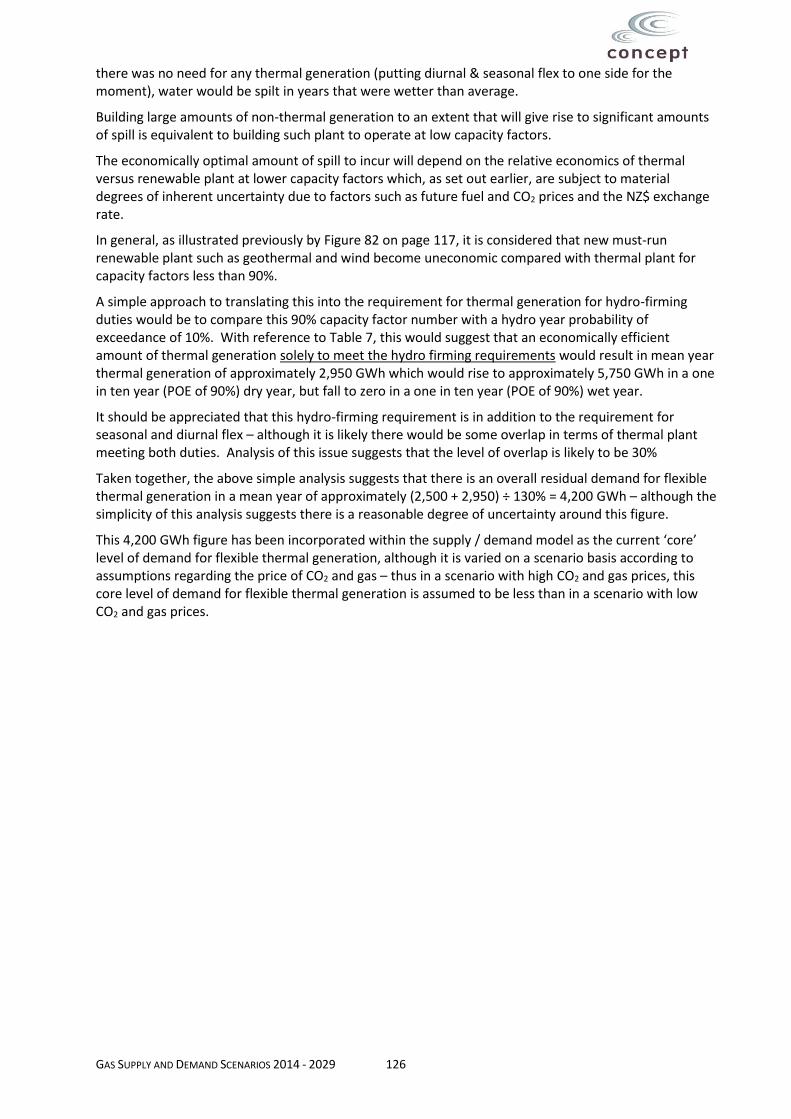
GAS SUPPLY AND DEMAND SCENARIOS 2014 - 2029 126
there was no need for any thermal generation (putting diurnal & seasonal flex to one side for the moment), water would be spilt in years that were wetter than average.
Building large amounts of non-thermal generation to an extent that will give rise to significant amounts of spill is equivalent to building such plant to operate at low capacity factors.
The economically optimal amount of spill to incur will depend on the relative economics of thermal versus renewable plant at lower capacity factors which, as set out earlier, are subject to material degrees of inherent uncertainty due to factors such as future fuel and CO2 prices and the NZ$ exchange rate.
In general, as illustrated previously by Figure 82 on page 117, it is considered that new must-run renewable plant such as geothermal and wind become uneconomic compared with thermal plant for capacity factors less than 90%.
A simple approach to translating this into the requirement for thermal generation for hydro-firming duties would be to compare this 90% capacity factor number with a hydro year probability of exceedance of 10%. With reference to Table 7, this would suggest that an economically efficient amount of thermal generation solely to meet the hydro firming requirements would result in mean year thermal generation of approximately 2,950 GWh which would rise to approximately 5,750 GWh in a one in ten year (POE of 90%) dry year, but fall to zero in a one in ten year (POE of 90%) wet year.
It should be appreciated that this hydro-firming requirement is in addition to the requirement for seasonal and diurnal flex – although it is likely there would be some overlap in terms of thermal plant meeting both duties. Analysis of this issue suggests that the level of overlap is likely to be 30%
Taken together, the above simple analysis suggests that there is an overall residual demand for flexible thermal generation in a mean year of approximately (2,500 + 2,950) ÷ 130% = 4,200 GWh – although the simplicity of this analysis suggests there is a reasonable degree of uncertainty around this figure.
This 4,200 GWh figure has been incorporated within the supply / demand model as the current ‘core’ level of demand for flexible thermal generation, although it is varied on a scenario basis according to assumptions regarding the price of CO2 and gas – thus in a scenario with high CO2 and gas prices, this core level of demand for flexible thermal generation is assumed to be less than in a scenario with low CO2 and gas prices.

GAS SUPPLY AND DEMAND SCENARIOS 2014 - 2029 127
Appendix B. Description of the model used to develop power generation projections
The modelling approach is as follows:
Future demand for electricity is projected on a scenario-based basis.
Four Tiwai demand scenarios are considered: High (being full site production), Medium (where demand is equal to minimum contract level plus 50% of the difference between full site output and the minimum contract level), Low (where demand is equal just to the minimum contract level), and Tiwai exit from 2018.
The scenario growth rates for rest of New Zealand demand are: High = 1.75%, Medium = 1.0%, Low = 0.25%
Growth in low-capacity factor demand is separately identified to baseload demand, using a framework based on the analysis set out in Appendix A.
The residual demand for thermal generation in a mean year is calculated as overall demand, minus the generation from existing hydro, geothermal, wind and cogen
The extent to which existing CCGTs meet growth in the residual demand for baseload thermal generation, versus being displaced by potential new renewable generation is undertaken via a simple scenario-based approach based on scenarios relating to CO2 costs (High, Medium and Low) and gas prices (being the main three gas market scenario futures set out in section 2.2.)
New renewables are assumed to be built if the capacity factor of the existing CCGTs rises above a threshold. In a future of low CO2 and gas prices, the threshold capacity factor is set to 85%, whereas in a future of high CO2 and gas prices, the threshold capacity factor is set to 0% - i.e. CCGTs are completely displaced from baseload operation by renewables, but will still operate to meet some of the demand for seasonal and diurnal flexibility. CO2 and gas market scenarios between these extremes have the threshold capacity factors set between these two levels. The exception to this is:
e3p whose high take-or-pay contract means it will continue operating at baseload for much longer, irrespective of the scenario. However, in the scarce gas scenario its capacity factor is assumed to drop significantly towards the latter part of this projection, as it is likely that Genesis will sell on the gas to other, higher value users.
scenarios where existing CCGTs have been retired or reconfigured – which is also a user-varying assumption as set out below.
It has been assumed that no new CCGTs will be built to meet growth in baseload demand due to the likely higher cost of CO2 which will be reflected on major emitters of CO2 in some fashion88.
Huntly and OCGTs are considered to be completely displaced from baseload duties in all scenarios, and only operate to meet the demand for flexible generation
There are assumptions as to the economic minimum quantity of thermal generation required to provide flexible generation to meet the seasonal & diurnal variation in demand, and to provide hydro-firming capabilities. This minimum economic quantity is based on the analysis set out in Appendix A. The extent of this is reduced for high CO2 and gas market scenarios – i.e. the threshold
88 There is a growing international consensus (as reflected in the latest IPCC report) that climate change is significant, and the social costs are likely to be materially higher than reflected in the current low levels of CO2 prices. What is not clear is whether and how these costs will be reflected in a cost to GHG emitters over the next 10-15 years. An assumption has been made that developers of CCGTs would be unlikely to take on this political risk and build a new CCGT, even if current CO2 prices are low.

GAS SUPPLY AND DEMAND SCENARIOS 2014 - 2029 128
capacity factor below which it is uneconomic to displace thermal generation with new renewables falls.
There is an assumption as to the absolute minimum quantity of thermal generation required to meet the seasonal & diurnal variation in demand (i.e. due to the renewable fleet being physically incapable of meeting all this variation due to the factors set out in Appendix A). This is required for consideration of scenarios where Tiwai completely exits New Zealand
The extent to which Huntly on coal meets the demand for flexible thermal generation versus gas-fired plant also varies according to the CO2 and gas price assumptions. It is assumed that Huntly will meet a greater proportion of the demand for thermal hydro-firming swing than the demand for flexible thermal to provide diurnal and seasonal flexibility.
If the demand for flexible generation to meet diurnal & seasonal duties increases above the capability of existing plant, it is assumed that new OCGTs will be built.
Users can simulate the effect of retiring or reconfiguring certain thermal plant including:
Retiring TCC
Re-configuring Otahuhu B to OCGT mode
Another variable is the extent to which Huntly generation is met by gas, rather than coal. Again, this is varied on a simple scenario basis based on the gas and CO2 price assumptions.
To test the plausibility of the numbers produced by the model in terms of GWh generation from the various different plant, and the resultant gas burn, some simple ‘back-casting’ was done in terms of feeding the actual residual demand for thermal generation in 2011 to 2013 into the model (which takes account of the extent to which these years were dry or wet) and seeing what the model produced in terms of PJ of fuel burn. This is necessary because the model is a mean hydro year model.
The results of this back-casting are shown below.
Based on this simple ‘sanity check’ it appears that the model is producing numbers which are ‘reasonable’ .

GAS SUPPLY AND DEMAND SCENARIOS 2014 - 2029 129

GAS SUPPLY AND DEMAND SCENARIOS 2014 - 2029 130
Appendix C. 2012 analysis of relationship between demand and sectoral GDP and population89
In seeking to understand what has driven changes in demand (with a view to developing a framework that could be used to project possible demand futures), some initial analysis was undertaken looking at factors such as GDP and population, given that these are two key drivers of the demand for energy services. Accordingly regional and sectoral data on both factors were sourced from Berl Economics and Statistics New Zealand, respectively.
However, as the following charts illustrate, no correlation of any significance could be identified which could be used as a basis for developing future projections.
The first set of charts grouped under the heading of Figure 91 shows GDP and gas demand for the different demand sectors on a whole of North Island basis. In addition to the main industry sectors of Dairy, Paper, Meat, etc, the final chart in this series looks at combined GDP for all other industry sectors and compares it with ToU demand.
Figure 91: Correlations between GDP and gas demand for different sectors for whole of NI
89 This analysis is largely unchanged from the 2012 study, except that the regional and sectoral growth rates in Figure 94 on page 98 have been updated to include the latest gas gate data.

GAS SUPPLY AND DEMAND SCENARIOS 2014 - 2029 131
In most cases there is little or no correlation, or sometimes an apparent negative correlation between economic activity and gas demand.
When the data is considered on a regional basis the picture is similarly confused. For example, the following two charts in Figure 92 show the correlation between other-industry GDP and TOU gas demand for the North System and the South system.
For the North System there appears to be a reasonable positive correlation. However, for the South System there appears to be an even stronger negative correlation.

GAS SUPPLY AND DEMAND SCENARIOS 2014 - 2029 132
Figure 92: Correlation between other-industry GDP and TOU gas demand on a regional basis
Nor does there appear to be a correlation between population and gas demand for the Non-TOU sector as illustrated by the charts grouped under Figure 93 below.
Figure 93: Correlation between population and gas demand for Non-TOU sector

GAS SUPPLY AND DEMAND SCENARIOS 2014 - 2029 133
In addition to suffering from only having eight years’ worth of data (which is really too little to do this type of statistical analysis), the likely explanation for this apparent lack of correlation between gas demand and GDP and population is because, for most uses, gas is readily substitutable with other fuels. This substitutability probably explains much of the apparent negative correlations observed above for the specific industry sectors. For example, it is understood the Paper sector has been progressively switching away from using fossil fuels as an energy source to burning on-site biomass, plus in some cases using geothermal resources that happen to be located at the sites. In the meat sector, on the other hand, there has been some switching away from coal to gas during a time when GDP for the sector was gradually declining.
And in the mass-market sector, it is understood that gas has been losing market share to electricity for space heating, as heat pumps have gained market share over the last decade.
This substitutability contrasts with electricity demand where, for a large proportion of its uses, it is not readily substitutable with another fuel (for example in lighting, appliances, etc.). As such, electricity demand exhibits a much greater correlation with factors such as population and GDP.
Because of the scope for substitution, the demand for gas is not just a function of the demand for energy services (which, for a specific industrial sector, is reasonably correlated with GDP), but is also a function of the relative cost of gas versus other fuel options for meeting such energy services. This relative cost is a function of a number of factors, including:
Wholesale fuel prices (gas, coal, diesel, LPG, biomass and electricity)
Fuel transport prices (including network costs for gas and electricity)
CO2 costs and CO2 intensities of the different fuels
End-use appliance / equipment characteristics
capital costs
operating costs
operating efficiencies
For the TOU sector, which covers a broad range of different industries, another complicating factor is that structural change within this broad ‘sector’ is influencing the demand for energy services. In other words, different types of industrial and commercial activities have been growing at different rates over the last couple of decades, and will likely continue to grow at different rates in the future. Given that these different types of industrial and commercial activities have differing levels of energy intensity, this structural change in the composition of New Zealand’s business sector will have a corresponding change in the demand for energy services and its apparent relationship with GDP.
Given all of the above, in order to project gas demand, it would also be necessary to take account of all these other factors.

GAS SUPPLY AND DEMAND SCENARIOS 2014 - 2029 134
Given the many different ‘moving parts’ driving gas demand, many with significant uncertainties, it would be extremely challenging to try and explicitly model possible demand growth based on projections of factors such as GDP, population, fuel prices, CO2 prices and the like.
In particular, trying to develop a statistical model which examined historical data series to infer the relationship between the combinations of all the above such factors and gas demand would face significant challenges, including:
The data series is likely to be too short (there is only ten years’ worth of reliable gas data) to develop any correlations of any real significance – in particular because it is likely that some relative cost states of the world that may occur in the future haven’t been experienced in the past (for example due to some technologies rapidly changing their costs or efficiencies, or CO2 / fuel prices that haven’t been experienced yet)
There is limited data for many aspects of the factors which make up the relative cost equation
The challenge in trying to project growth rates for different sectors on a regional basis is highlighted by considering historical data as illustrated by the table below.
Figure 94: Historical annualised gas demand growth rates for different sectors and different regions (updated for 2014 study)
There have been significant variations in growth rates across different periods, and across different Systems for the same types of demand. It would not be feasible to develop a statistical model which could reliably forecast such changes.
Accordingly, this study (and the associated publically available model) takes the approach of developing gas demand projections which are based on observed historical trends, but informed by high-level analysis of the economics of the main uses for gas relative to the main competing fuels / technologies.

GAS SUPPLY AND DEMAND SCENARIOS 2014 - 2029 135
Appendix D. Description of statistical model Due to the inherent variability of demand driven by factors such as the weather, and ‘natural’ randomness in the coincident level of demand from consumers, this necessarily requires the ability to consider the probabilities of peak demand reaching certain levels, and thus be able to estimate what a 1-in-20 year or 1-in-50 year level of peak demand would be. This exercise has some key inherent challenges:
There is only a limited historical gas demand data set (just over ten years), meaning that just considering this data alone would make it hard to infer what a 1-in-50 year peak demand, say, might look like;
There is a need to be able to consider peak demand over different lengths of time, ranging from a day through to a week, given that the critical time-period for different pipelines can vary;
Different demand sectors exhibit different seasonal and diurnal patterns, and different temperature sensitivities, yet the proportions of these different sectors has varied during the historical data series, and is likely to vary further into the future.
To address these issues, a statistical model was developed which sought to determine the relationship between demand and key observable drivers (namely temperature and temporal parameters (for example day of week, month of year, public holidays)).
Figure 95 below shows how different sectors exhibit different degrees of seasonal and diurnal variation.

GAS SUPPLY AND DEMAND SCENARIOS 2014 - 2029 136
Figure 95: Examples of different patterns of seasonal and diurnal demand for different sectors in the North System90
90 For this year ending November representation, Day 1 = 1st December, and Christmas = Day 25.

GAS SUPPLY AND DEMAND SCENARIOS 2014 - 2029 137

GAS SUPPLY AND DEMAND SCENARIOS 2014 - 2029 138
As can be seen, mass-market customers (represented by the ‘Non’ (i.e. non-time-of use) category) have a strong seasonal pattern to their consumption driven by the space heating requirement in winter.
Dairy customers also have a very strong seasonal pattern to their consumption. However, unlike mass-market customers, this is not driven by winter-temperatures for space heating, but rather the seasonal variation of cows producing milk. As it happens, this tends to mean that dairy users have a counter-cyclical consumption profile, such that their proportionate contribution to the system peak is much less than their proportionate contribution to overall annual demand.
General business customers (as represented by the ‘Tou’ (i.e. time-of-use) category) have a strong weekday / weekend pattern to their consumption, but with less of a seasonal variation – apart from a significant reduction in consumption during the Christmas holiday period. This is because of their work patterns, and the fact that the majority of their gas requirement is for process heat which is not affected by temperature.
The steel sector (represented by the Gleenbrook steel mill) shows quite a degree of random variation, presumably relating to the continual cycle of production runs. Despite, or perhaps because of, this randomness, its consumption record is well suited to statistical analysis to consider the likelihood of different levels of gas consumption.
The power generation sector, on the other hand, does not appear to be well suited to the type of statistical analysis that would be appropriate for the other sectors. This is because the gas-fired power generation outcomes observed during the past ten years are due to a range of factors including changes in wholesale fuel prices, swing fuel prices, fuel contracts, CO2 prices, electricity transmission constraints, and the variability in other forms of generation (particularly hydrology and more recently wind).
Many of these factors experienced material changes during the course of the last ten years, and are projected to undertake even more significant changes in the following decade. This will greatly reduce the relevance of statistical analysis of the last ten years’ outcomes as a means of considering potential outcomes for the next ten years.
In addition, as set out in more detail in section Appendix E, it is considered that the electricity generation sector probably has the greatest potential to economically respond to altered price signals to reduce consumption during the relatively infrequent times of pipeline congestion.
Given all of the above, no statistical analysis was performed on the generation sector.
With respect to sensitivity to temperature, the issue is that space heating demand can vary significantly with the weather, and the weather itself can vary significantly from year-to-year. Thus, peak heating demand in a year with a particular severe cold snap can be significantly higher than in a relatively mild year. This makes it challenging to project peak demand, and means that any projections must be made with reference to a particular probability of weather-severity. For example, a 1-in-20 year peak demand means the demand that would be expected during a weather event whose severity would only be expected once every 20 years.
To illustrate the sensitivity of demand to weather, Figure 96 below shows how Non-Tou demand varies with temperature for the North system91.
91 Slightly counter-intuitively, it was discovered that demand was better correlated with daily maximum temperature rather than daily minimum temperature. This could be because a large proportion of heating occurs during the day and evening, and maximum temperatures are likely to be a better proxy for day / evening temperatures than minimum temperatures (which are most likely to occur in the early hours of the morning).

GAS SUPPLY AND DEMAND SCENARIOS 2014 - 2029 139
Figure 96: Relationship between Non-Tou demand in the North system and temperature
Source: Concept analysis
As can be seen, as temperature drops, Non-Tou demand increases. However, some sectors exhibit little or no temperature sensitivity to demand due to the fact that their gas is used for industrial processes rather than space heating. This is illustrated in Figure 97 below which shows that demand for gas for Steel manufacture has little correlation with temperature.
Figure 97: Relationship between gas demand for the Steel sector in the North system and temperature

GAS SUPPLY AND DEMAND SCENARIOS 2014 - 2029 140
Source: Concept analysis
As an aside, the analysis also revealed that the cold snap of the week of 15-19 Aug 2011 (and associated gas demand peak) really was unusual. On a rolling 5 day maximum temperature basis, the weather during 15-19 August was ≈ a 1 in 95 year event (using 46 years’ worth of temperature data, and a Generalised Extreme Value (GEV) probability distribution approach). This is illustrated in Figure 98 below.
Figure 98: Distribution of annual minimum values for rolling 5 day maximum temperatures
Given that different sectors exhibit different seasonal and diurnal patterns in demand, and differing levels of temperature sensitivity, the key problem in determining what a 1-in-20 or 1-in-50 peak gas demand might look like is that:
There is only a limited historical gas demand data set (just over ten years). Thus, looking at this data alone would make it hard to infer what a 1-in-50 year peak demand, say, might look like; and
The relative proportions of different gas sectors has changed over this time (for example the proportion of Tou versus Dairy, say).
To address both of these issues, plus the issue of different sectors exhibiting different seasonal and diurnal variations in demand, a statistical model was developed which sought to determine the relationship between temperature and key temporal parameters (for example day of week, month of year, public holidays).
This model was based on ten years’ worth of historical daily gas demand and ambient temperature data, and considered each of the different sectors separately. i.e. a statistical relationship was developed for the Non-tou sector, the Tou sector, and each of the sectors such as Meat, Dairy, etc.
The model is a linear regression model, implemented in the R programming language. It sought to determine the best algorithm which could be used to explain observed demand when linked to observed other factors (such as temperature, day-of-week, etc.).
This algorithm could then be fed a more comprehensive set of historical daily temperature data to enable development of a more comprehensive set of possible demand futures for each demand sector.
9 10 11 12 13 14
0.0
0.1
0.2
0.3
0.4
0.5
Yearly Minimum Daily Maximum Temperature (C)
pd
f
Distribution
Historical Minimums
2011

GAS SUPPLY AND DEMAND SCENARIOS 2014 - 2029 141
The model is expressed as:
Daily demand =
Coefficient varying from year to year + Trend component
Coefficient depending on month, day of week, and public holiday or not + Cyclic component
Quadratic function of today’s maximum temperature* + Temperature component (if applicable)
Quadratic function of tomorrow’s maximum temperature* +
Whatever is left Residual component
* or 18 degrees, whichever is less. Demand does not tend to increase further past this point
This model was selected from a reasonably wide pool of alternatives on the basis of good explanatory power + simplicity. For instance we considered min temperature rather than max, and yesterday’s temperature rather than tomorrow’s, but neither was an improvement. In both cases this is probably because heating needs are driven largely by evening temperatures, which are more correlated with the following day than the previous day, and more likely correlated with the maximum demand during the day than the minimum demand during the night.
Here is an example of how the decomposition works for non-ToU demand in the North system.
Here is the trend component (showing little trend over time, but a possibly anomalous value for 2002). This trend component is required to effectively normalise the data to account for changing overall quantities of demand over time due to changing numbers of consumers on the network.
The cyclic component is harder to show because it’s made up of 168 values – 12 months of the year x 7 days of the week x (weekday or not). However, here are some summaries of it.
Looking just at months, we see demand being highest in winter, driven by increased space heating requirements in the winter months.

GAS SUPPLY AND DEMAND SCENARIOS 2014 - 2029 142
The model allows the shape over the week to vary from month to month. However, looking across all
months, we see demand being highest on weekdays (as one would expect):
And naturally demand is low on public holidays.

GAS SUPPLY AND DEMAND SCENARIOS 2014 - 2029 143
The temperature component is demonstrated in the plot below:
After all these components have been stripped out, only the residual component remains which represents that element of observed demand which cannot be explained by the other factors, and characterises the random variation that will occur ‘naturally’. This is largely noise, with a small amount of day-to-day correlation.
A statistical model was developed for each demand sector for each geographic region. For the major industrial sectors (i.e. all sectors apart from the Non-TOU and TOU sectors), no correlation with temperature was observed. Accordingly, for such sectors, no temperature component has been included in the statistical model.
Once the statistical relationships had been determined, for those sectors for which a material sensitivity to temperature had been established (only the Non-TOU and TOU sectors), the model was then fed 45 years’ worth of historical daily temperature data. This produced daily demand projections of what gas demand would likely have been like for each of these 45 years for each of the sectors. In fact, for each of these 45 historical ‘temperature years’, ten yearly demand projections were produced due to the observed ‘noise’ in the ten years’ worth of historical data which can’t be exactly explained by temperature or temporal dependencies, but are representative of the random variations in demand that will naturally occur.
-5,000
-4,000
-3,000
-2,000
-1,000
0
1,000
2,000
3,000
Re
sid
ual
De
man
d (
GJ)

GAS SUPPLY AND DEMAND SCENARIOS 2014 - 2029 144
For the sectors which didn’t have any material sensitivity to temperature, only ten years of daily demand projections were produced, based on the temporal drivers determined in the model and factored by the ‘noise’ observed in the ten years of historical data.
Figure 99 below shows an illustration of one such set of projections for one sector.
Figure 99: Example projections of daily Non-Tou demand for the North System for a sub-set of possible future years92
With these 450 modelled years’ worth of data it is possible to get better insights into the variability of gas demand for the different sectors, and the probabilities of different levels of peak demand.
For example, Figure 100 below illustrates that the Non-TOU sector has a few days of extreme peak demand.
92 For ease of illustration, only 40 daily profiles are shown in this graph. In reality, 450 profiles are produced by the model, corresponding to the 45 historical temperature years, combined with each of the ten ‘residual’ years for which historical data exists.

GAS SUPPLY AND DEMAND SCENARIOS 2014 - 2029 145
Figure 100: Duration curve of modelled gas demand for Non-Tou sector for North system over a 45 year time-frame
It is also possible to get analysis on the likelihood of a particular level of peak demand being observed in a year.
To illustrate this Figure 101 below shows just five daily projected demand profiles from the model. (Noting that 450 demand profiles would be produced for a temperature-sensitive sector, and 10 for a non-temperature sensitive sector).
For each of these five profiles, the peak day demands have been circled. As the text box in the diagram shows, the average of these five peak days is 25,241 GJ, the maximum is 28,438 GJ and the minimum is 23,257 GJ. Thus, if only these five profiles were available, the 1-in-5 year peak demand would be approximately 28,438 GJ, and the mean peak demand would be 25,241 GJ. Of course, with greater numbers of demand profiles than 5, it is possible to derive more statistically significant peak demand probabilities.

GAS SUPPLY AND DEMAND SCENARIOS 2014 - 2029 146
Figure 101: Illustration of derivation of peak demand levels
It is also possible to use such daily demand profiles to calculate peak week demands and the probabilities of differing levels of peak week demands using the same approach as described above.
Figure 102 below illustrates the probabilities of differing levels of peak day and peak week demands based on the statistical output from the model for one particular sector.

GAS SUPPLY AND DEMAND SCENARIOS 2014 - 2029 147
Figure 102: Example of probabilities of differing levels of peak day and peak week demand for the Non-TOU sector for the North system for 2012

GAS SUPPLY AND DEMAND SCENARIOS 2014 - 2029 148
Appendix E. Interruptibility
If demand for a network exceeds the available capacity that is able to be supplied, one option to relieve such a situation is to invest to increase the network capacity.
However, another option that may be more economic is for some consumers to elect to curtail their demand at times of peak, thereby enabling other consumers who value the gas more highly to satisfy their demand. Such voluntary interruption of demand by some consumers to relieve the peak could postpone the need for capital-intensive network investment.
Allowing customers to elect to interrupt demand could potentially be a more cost-effective solution than network investment if:
The peak period is for a relatively short amount of time; and/or
There are some consumers whose value of demand is significantly lower than others; and/or
Network investment is relatively expensive.
With regards to the first point, Figure 103 illustrates that times of peak stress occur relatively infrequently on the Northern System, thereby raising the potential for some consumers demand to be curtailed for relatively short periods of time in order to help relieve such congestion.
Figure 103: Duration curves of historical total daily gas demand on Vector North system
With regards to some customers potentially having a relatively low value of load, numerous studies have been undertaken of the value of load for different types of customer for both the electricity and gas sectors. They reveal major differences in the value of energy to different groups of customers, and raise the potential for some customers to economically curtail their gas demand for relatively short periods at peak, rather than invest in extra pipeline capacity.
In addition to these differences in customers’ ‘inherent’ value of gas, there may also be significant opportunities for some customers to curtail their demand for a short period of time because the energy service could be satisfied by a back-up fuel option.

GAS SUPPLY AND DEMAND SCENARIOS 2014 - 2029 149
From discussions with stakeholders, it is apparent that there is some potential for both types of gas interruption from a number of different customers:
Some consumers indicated that they had some relatively low value processes on their site which they may be able to curtail for relatively short periods of time without incurring excessive cost; and
Some consumers indicated that they have back-up energy options which they could switch to such as diesel. Indeed, it is understood that a number of these back-up energy options have been put in place following the 2011 Maui pipeline outage.
Some consumers indicated that they felt there was significant potential for interruption at times of peak to manage pipeline capacity issues, but that there was not currently a strong enough price signal for them to deliver such interruptible potential. Indeed, to-date it is understood that only a handful of customers currently have an interruptible pipeline contract with Vector:
the refinery at Marsden Point93
the gas-fired power stations at Otahuhu and Southdown.
Analysis was undertaken to determine whether demand interruption could indeed make a more significant contribution to managing pipeline capacity constraints, with a particular focus on the North System. If demand interruption was revealed to potentially be an economic option, it could have a major bearing on future levels of peak gas demand. The analysis focussed initially on gas used for power generation.
Interruptibility from power generators
As shown Figure 104, gas used for electricity generation is the biggest contributor to peak week demand on the Vector North system.
93 Under the terms of this contract, Vector can interrupt flows of gas to the refinery at times of pipeline capacity constraint. In return, the refinery pays a lower $/GJ fee than other users of the pipeline who have an uninterruptible contract. Vector calls upon this interruption to manage congestion on the whole of the North system, as well as more localised congestion in the pipeline north of Auckland. It is further understood that the refinery can manage such interruption primarily by switching to an alternative fuel during such periods (essentially diverting hydrocarbons away from being processed into an end product, and instead burning them as an input fuel).

GAS SUPPLY AND DEMAND SCENARIOS 2014 - 2029 150
Figure 104: Historical sectoral composition of peak week demand for Vector North system (GJ)
Figure 105 gives more insight as to the type of operating pattern being undertaken by the two gas-fired generators in the North System (Otahuhu B and Southdown) during these peak weeks.
Figure 105: Otahuhu B + Southdown hourly gas consumption during YE June peak weeks
During the daytime the generators were operating at close to full capacity, but reducing demand during the night. In some cases there appears to have been some demand reduction during the mid-

GAS SUPPLY AND DEMAND SCENARIOS 2014 - 2029 151
day period, but not down to overnight levels. During the 2008 peak week (which was during an electricity hydro-shortage) there appears to be hardly any reduction at all.
One issue that was considered was whether there was potential for the two Auckland-based generators to reduce their generation (and hence gas demand) even further during peak week periods in order to free-up some pipeline capacity. Such an option would only be feasible if there was other generation capacity elsewhere on the New Zealand electricity system which could replace this lost generation. An indicative simplified analysis suggests that from a generation capacity perspective, this is indeed the case.
For this analysis it was assumed that there would be a strong correlation between periods of peak gas demand and peak electricity demand. The analysis then looked at the hourly electricity demand during the peak week of gas demand. The (conservative) assumption was made that during the hour of highest demand in this week the electricity system would be running at capacity, and thus could not afford to lose any generation from Otahuhu B and Southdown. However, it was assumed that as demand fell from this level, it would be possible for Otahuhu B and Southdown to similarly scale back.
Figure 106 below shows how national electricity demand varied during the 2010 peak gas week. A horizontal red line is also shown corresponding to the peak electricity demand level minus Otahuhu B + Southdown’s capacity. Thus, using the conceptual framework above, when electricity demand rises above this level Otahuhu B + Southdown would be needed by that amount, but when it is below this level they would not be needed.
This level of ‘need’ is indicated by the bottom green line in the figure – i.e. essentially only operating to meet the morning and evening peaks during the weekdays. For comparison, the purple line shows the actual level of generation by the two Auckland generators which is much higher than this simple level of need. This suggests that there could be significant potential for the Auckland-based generators to reduce their generation at times (for example overnight) during the peak gas weeks to free-up gas pipeline capacity.
If the generators were to follow this line of ‘need’ in the diagram, the amount of gas capacity that would be freed up would be equal to the area between the purple and the green lines. This would reduce generation (and consequent gas demand) by 85% during the Monday to Friday period.
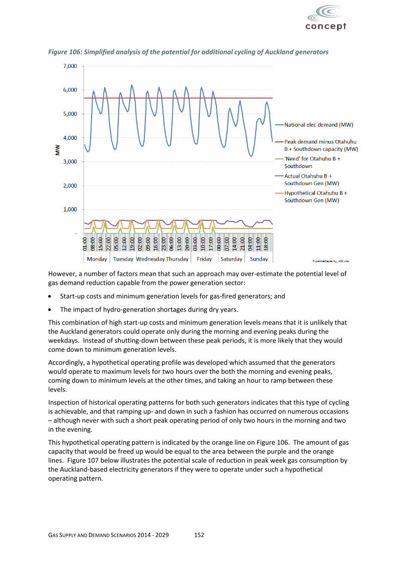
GAS SUPPLY AND DEMAND SCENARIOS 2014 - 2029 152
Figure 106: Simplified analysis of the potential for additional cycling of Auckland generators
However, a number of factors mean that such an approach may over-estimate the potential level of gas demand reduction capable from the power generation sector:
Start-up costs and minimum generation levels for gas-fired generators; and
The impact of hydro-generation shortages during dry years.
This combination of high start-up costs and minimum generation levels means that it is unlikely that the Auckland generators could operate only during the morning and evening peaks during the weekdays. Instead of shutting-down between these peak periods, it is more likely that they would come down to minimum generation levels.
Accordingly, a hypothetical operating profile was developed which assumed that the generators would operate to maximum levels for two hours over the both the morning and evening peaks, coming down to minimum levels at the other times, and taking an hour to ramp between these levels.
Inspection of historical operating patterns for both such generators indicates that this type of cycling is achievable, and that ramping up- and down in such a fashion has occurred on numerous occasions – although never with such a short peak operating period of only two hours in the morning and two in the evening.
This hypothetical operating pattern is indicated by the orange line on Figure 106. The amount of gas capacity that would be freed up would be equal to the area between the purple and the orange lines. Figure 107 below illustrates the potential scale of reduction in peak week gas consumption by the Auckland-based electricity generators if they were to operate under such a hypothetical operating pattern.

GAS SUPPLY AND DEMAND SCENARIOS 2014 - 2029 153
Figure 107: Illustration of potential scale of reduction in peak week gas consumption94
Based on this hypothetical profile, demand for gas from electricity generators could be 160 TJ/week less than occurred during the 2012 YE June peak week (which occurred in the cold snap of August 2011). By way of a comparison, 160 TJ/week represents 20% of pipeline capacity on the North System.
The analysis on page 152 considers the ability of the electricity system to replace any lost generation from Otahuhu B and Southdown purely from a generating capacity perspective. However, at times of hydro shortage, it is possible that the Auckland-based generators may be needed at all times during the peak gas week, not just during the morning and evening periods of peak demand.
To consider whether this may be the case, a simple analysis was undertaken which compared wholesale electricity prices during the 2008 peak week (which was at the height of one of the most severe hydro shortage periods in the last 15 years), with an inferred value for pipeline capacity at times of peak.
As shown in Figure 108, during the 2008 dry period, electricity prices were generally around $300/MWh, sometimes rising to approximately $500/MWh. In other years with more normal hydrology, prices were lower – typically between the $80 to $120/MWh level95. On average, during peak gas week periods, electricity prices have fluctuated between $100/MWh to $380/MWh, and averaged around $160/MWh.
94 The data is organised in years ending June, rather than November as in the rest of the analysis, because it sources data published by Vector in its annual capacity statement which publishes such information on a year ending June basis. 95 It should be noted that the YE June 2009 gas peak week actually occurred in July 2008, when the hydro shortage event was still being experienced.

GAS SUPPLY AND DEMAND SCENARIOS 2014 - 2029 154
Figure 108: Wholesale electricity prices at Otahuhu during peak gas weeks
To infer a value for pipeline capacity at times of peak, a simple calculation was undertaken which comprised a number of steps:
Estimate the annual revenue Vector collects from transmission tariffs on the North System. This was assumed to be broadly representative of the long-run cost of providing pipeline capacity. (i.e. both recovery of operating and capital costs). Based on Vector’s published tariffs and information about gas demand on the North System, this annual revenue was estimated to be approximately $55 million.
Divide this number by the GJ capacity of the pipeline at times of peak. The resulting $/GJ figure can be considered representative of the costs of providing peak capacity96. Two calculations were undertaken for the North System:
Dividing the annual revenue by peak day capacity = $330/GJ
Dividing the annual revenue by peak week capacity = $66/GJ
As a cross-check, these numbers were compared with numbers produced in a 2009 study published by Gas Industry Company97. Table 7 of this study, reproduced as Table 8 below, shows estimates of the marginal cost of expansion (MCE) for a number of different pipeline expansion options.
96 It should be caveated that this simple framework assumes that the cost of providing pipeline services is predominantly driven by having sufficient capacity to meet peak demand. This is an over-simplification in that there are other costs driving the provision of pipeline services. However, it is understood that peak demand is the principal driver behind the pipeline investment costs. As such, it is considered that this approach gives a reasonable indication of the scale of costs of providing pipeline services at times of peak. 97 “Review of Vector capacity arrangements A research paper” Creative Energy, January 2009 http://gasindustry.co.nz/sites/default/files/publications/Vector_Capacity_Research_Paper_149282.2.pdf

GAS SUPPLY AND DEMAND SCENARIOS 2014 - 2029 155
Table 8: Assessment of MCE on Vector transmission network
Pipeline Delivery point Description of expansion Cost ($m) Inc TJ MCE ($/GJ/yr)
North Westfield Pap East to Smales Rd North loop 26.7 116 23
Whangarei Pap East to Smales Rd loop 26.7 16 167
Central North Morrinsville Horotiu compression 11.9 42 28
Bay of Plenty Kinleith upgrade Pokuru compressor 16.1 24 68
Gisborne upgrade Pokuru compressor 16.1 21 77
South South Tawa upgrade Kaitoke, loop to Hima 39.8 105 38
South Hastings upgrade Kaitoke, loop to Hima 39.8 68 58.5
As can be seen, the estimates produced via the peak week calculation set out above appear reasonable when compared with the MCE values shown in Table 8.
These gas transport costs were added to an assumed gas wholesale price of $10/GJ (which includes an assumed cost of swing for delivering peak gas), and then multiplied by the heat rate of a CCGT, which was assumed to be 7.1 GJ/MWh. The resulting figures were:
$2,400/MWh when using a peak day measure of capacity; and
$540/MWh when using a peak week measure of capacity.
These $/MWh figures represent the required electricity price to justify the use of gas-fired power generation (and thus using up scarce pipeline capacity) during these peak periods.
In other words, if the value of electricity during these peak week periods was higher than this inferred cost of providing gas pipeline capacity, then it would be economically efficient to invest to provide such pipeline capacity. However, as can be seen by comparing the electricity prices in Figure 108 with the above inferred pipeline capacity cost figures, they typically do not reach such levels.
This would tend to imply that it would not be economic to invest in pipeline capacity to enable uninterrupted gas-fired electricity generation during the gas peak week – even to accommodate infrequent dry years.
As such, it would appear that interruption of gas-fired generation would be economic during peak weeks to manage pipeline scarcity issues, even taking into consideration the elevated value of electricity during dry-year periods. Accordingly, any framework for projection of gas demand on the Northern System should consider the potential for increased levels of such interruption.
It is understood that the Gas Industry Transmission Access (GITA) working group is considering the issues of access and capacity pricing arrangements, including how to incentivise interruptibility of gas-fired electricity generators where it is economic to do so.
Given the inherent uncertainty as to the eventual form of such arrangements, it is not considered that altered gas consumption patterns due to increased interruptibility could be subject to any detailed modelling for the purposes of the peak demand projections in this study. Rather, it is considered that a scenario basis be adopted for simulating the level of gas interruption, informed by the analysis described above considering the possible scale of such interruption.
Interruption from other consumers
In this respect, while the above analysis has focussed on the potential scale of interruption from electricity generators, it is also considered that some industrial users could deliver interruptible gas through the use of back-up fuel sources or curtailing production in some cases if they faced the price signals to do so.

GAS SUPPLY AND DEMAND SCENARIOS 2014 - 2029 156
In the case of switching to back-up fuel, it is considered that it would be economic to switch to burn diesel at ≈ $25/GJ, rather than incurring gas pipeline and wholesale costs of approximately $76/GJ as calculated above.
However, little quantitative information is available to enable firm estimates of the scale of this potential. Qualitatively, one industrial stakeholder who was installing diesel back-up capabilities following the Maui pipeline outage suggested that it was a relatively inexpensive investment. However, another suggested that the nature of their process meant it was harder to achieve.
Similarly, there was a mix of views as to the ease / cost of interrupting production for their different processes. Some indicated that their sites did have potential, whereas others indicated that the cost would be too great.
This variability in the responsiveness of different consumers to price signals is consistent with observed outcomes from directly-connected electricity consumers following the introduction of regional coincident peak demand charging for electricity transmission. Some consumers have been observed to radically reduce their consumption at times of peak (by more than 90%) following the introduction of this charging approach, while others have shown relatively little change to their consumption patterns.
Given this lack of firm data, simple assumptions have been made as to the potential for interruption from the other sectors. Thus it is assumed that these other industrial sectors could reduce peak week consumption by 15% (through a mixture of switching to diesel and interrupting processes) except for the Non-TOU, Dairy and Refining sectors where it is assumed that no potential for interruption (or further interruption in the case of Refining98) exists.
98 The refinery already has an interruptible contract with Vector. It is assumed that the maximum amount of interruption would have been called during the 2011 peak week incident.
Related Documents